Electoral Studies (1991). 10:2, 99-l 17

Modelling Trends in the Class/Party Relationship 1964-87

GEOFFREY EVANS*

Nuffield College, Oxford and The London School of Economics G Political Science

ANTHONY HEATH

Nuffield College, Oxfwd OXI Iln;, England

CLIVE PAYNE

Nuffield College, Oxford

Discussions of the nature of changes in the class/party association have focused on the theses of ‘trendless fluctuation’ and gradual decline in the class basis of British politics. This paper advances this debate by demonstrating that log-linear modelling can be used to test for more complex patterns of change over the period in question. In an analysis of the class/party association over eight elections both the trendless fluctuation and the gradual change thesis are shown not to fit the data particularly well. Far better fits are obtained by modelling the effects of political rather than sociological influences. Thus incumbency is shown to have a considerable impact on the class basis of support for the parties. Labour Party incumbency is shown to have an especially large effect in reducing the working class basis of support for the party. The paper both elaborates upon the methodological advantages of log-linear modelling and argues for new approaches to understanding the class/party relationship.

In the 1950s and 1960s few commentators challenged Pulzer’s claim that ‘class was

the basis of British politics while all else was embellishment and detail’ (Pulzer,

1968). Butler and Stokes in their work on the 1964 and 1966 elections developed the notion that class was ‘pre-eminent among the factors used to explain party allegiance in Britain’ (Butler and Stokes, 1974) and most observers appeared to

accept Lipset’s claim that ‘politics is the democratic translation of the class struggle’ (Lipset, 1960).

Since then it has become customary to claim that the class basis of British politics

has declined. Thus Crewe introduced the notion of class dealignment (Crewe et al., 1977) while Rose and McAllister (1986) talk about a change from closed class to open elections in Britain. In this way, the decline of class is seen to be associated

*This paper was presented at the workshop on ‘Social Structure and Electoral Change in Liberal Democracies’, European Consortium for Political Research joint sessions, Paris, lo- 15 April 1989

0261-3794/91/02/0099-191103 00 @ 1991 Butterworth-Heinemann

100 Modelling Trends in the Class/Party Relationship 1964-87

with a change in the social psychology of the voter; it is held that voters are now more inclined to vote on the basis of current issues or government record rather than on the basis of traditional group loyalty. It is thus part of a general thesis about dealignment and volatility.

These alleged changes are held to have important implications for British politics. Thus Franklin ( 1985) talks about the way in which the decline of class opened the way to radical change-in particular the rise of the Liberal Party in 1974. Franklin and others hold that the decline of the class basis of voting has removed the ‘cement’ which gave the British two-party system its stability. The British electorate is now wide open to change.

The explanations advanced by Crewe, Franklin, and Rose and McAllister for the decline of class voting tend to focus on the sociology of class; rising living standards and the spread of affluence has eroded working class values and ethos; the decline of traditional communities and increased social mobility have undermined class solidarity and led to more privatized, individualistic and instrumental voters; the emergence of new cross-cutting cleavages (both structural and ideological) have fragmented the social classes.

However, the decline could also be explained politically: it could be that the parties have changed their character. The main ‘class parties’ might have changed their electoral strategies, for example targeting different social groups (Przeworski and Sprague, 1986; Heath and Evans, 1988) or they may have become less successful than before in advancing the class interests that they were supposed to represent (Hibbs, 1982; Heath, Jowell and Curtice, 1985).

In this paper we shall not look at these explanations in detail as we shall be examining expanatory issues in a separate publication (Heath et al., 1991). Rather, we are mainly concerned with the modelling of the class/vote relation. That is to say, how can the changing association between class and vote over time best be represented? In what sense has there been a decline in class alignment? Has it taken the form of a gradual and continuous decline, as implied by the sociological thesis of a change in the character of the social classes? Or have the changes been more of a discontinuous form that might be related to political factors?

Approaches to the Measurement of Dealignment

The main evidence brought forward in favour of the class dealignment thesis has been (i) the decline in absolute class voting, that is the percentage of the electorate voting for their class party (in effect middle-class conservatives plus working class labour voters as a percentage of the electorate) and (ii) the decline in relative class voting, that is, the weakened association between an individual’s class position and voting behaviour. In these analyses class has typically been treated as a dichotomy- manual and non-manual-with individuals assigned to classes on the basis of head of household’s class. The association between classes and parties has usually been measured by simple summary coefficients such as, for example, the correlation coefficient or the Alford Index. Table 1 presents the relevant evidence for the 1964- 87 period, the period covered by the British Election Studies (which constitute our data sources ) ’

The distinction between absolute class voting and relative class voting is an important one. It is quite clear from Table 1 that absolute class voting has declined. In this respect there has been a real change in British politics-fewer people vote

GEOFFREY EVANS. ANTHONY HEATH AND CLMZ PAYNE 101

TABLE 1. The relationship between class and party using a dichotomized class schema 1964-87

1964 1966 1970 Feb 1974 Non- Non- Non- Non-

manual Manual manual Manual manual Manual manual Manual % % % % % % % %

Conservative Liberal Iabour

Non-manual Conservatives and manual tabour as % of all voters Odds ratio Alford Index

62 28 60 25 64 33 53 24 16 684 14 6 11 9 25 19 22 26 69 25 58 22 57

100 100 100 100 100 100 100 100

63 66 60 55 6.4 6.4 4.5 5.7

42 43 33 35

Ott 1974 1979 1983 1987 Non- Non- Non- Non-

manual Manual manual Manual manual Manual manual Manual % % % % % % % %

Conservative Liberal Labour

Non-manual Conservatives and manual Labour as % of all voters Odds ratio Alford Index

51 24 60 35 55 35 54 35 24 20 17 15 28 22 28 21 25 57 23 50 17 42 18 44

100 100 100 100 100 100 100 100

54 55 47 47 4.8 3.7 3.9 3.6

32 27 25 26

for their ‘natural class parties’. However, it is also apparent that this decline is temporarily associated with the rise of the Liberal Party (later the Alliance). Other things being equal, a rise in the voting strength of the Liberals (who are usually defined to be a non-class party) must Zogicully lead to a decline in absolute class voting. But of course we cannot use the decline in absolute class voting to explain, for example, the rise of the Liberals since the two are logically related. We cannot decide from this evidence whether it was the decline of class which opened the way to the rise of the Liberals or the electoral popularity of the Liberals which reduced class voting.

For this reason, Heath, Jowell and Curtice (1985) introduced the notion of relative class voting, which they measured with odds ratios. They defined relative class voting as the association between class and vote net of the overall shares won by the parties. In other words, they controlled statistically for the changes in the overall shares of the vote won by the parties to see if, net of these changes, the association between class and party had become weaker. This approach means that

102 Modelling Trends in the ClasslParty Relationship 1964-87

the share of the vote won by the Liberals becomes logically distinct from the level of relative class voting, and it therefore becomes sensible to ask whether there is a causal link between them. The basic idea is that, if class is indeed becoming a weaker force in shaping the way in which people vote, then this should show up even after

controlling for the overall vote won by the parties. Putting the matter slightly differently, has Labour lost votes in all classes equally thus retaining its character as a class party, albeit an unsuccessful one, or has it lost votes particularly in the working class, its voters thus becoming more of a cross-section of the electorate?

Most other commentators have also made distinctions akin to that between absolute and relative class voting, although their measures of relative class voting have not been entirely satisfactory. For example, the correlation coefficient fails to

distinguish between changes in the strength of the relationship between class and vote and changes in the relative sizes of classes or in overall levels of support for political parties. In particular, because of their dependence on the distributions of their constituent variables (i.e. classes and parties), correlation coefftcients will be affected by the decrease in the size of the working class during the 1964-87 period and by the changing distribution of the vote across the elections.

One approach to addressing the problems of the correlation coefficient has been to use unstandardized regression coefftcients to summarize the class-vote association. However, OLS regression assumes that the dependent variable (party) is a continuously measured variable with a normal distribution and homoscedastic error variance (these assumptions apply regardless of whether standardized or unstandardized coefficients are used). When the dependent variable is of only two unequal categories (e.g. labour vote vs non-labour vote) these assumptions are not being met. Therefore, although it is often the case that regression analyses give reasonably accurate estimates even when such assumptions fail to hold, in the case of dichotomous dependent variables (especially when the distributions are heavily skewed) the problems are considered to be sufficiently extreme to require special techniques such as logistic regression (Cox, 1970; Aldrich and Nelson, 1984). As discussions of class-vote dealignment often hinge upon quite small changes in the associations, the use of accurate estimation techniques is especially important.

It should be noted that, in the case of the two-class two-party model the Alford index is formally equivalent to the unstandardized regression coefhcient and thus must suffer from the same drawbacks. Just as OLS regression gives reasonably accurate estimates when the dependent variable is relatively unskewed, so the Alford index is a reasonable approximation when votes are divided more or less evenly between the two main parties. However, as the distribution becomes more skewed, the use of the Alford index becomes more problematic. In effect, ‘floor’ and ‘ceiling’ effects come into operation thus limiting the value which the index can reach. Thus as a party’s votes decline in number (that is, as the dependent variable becomes more skewed), it becomes mathematically impossible for the Alford index to remain constant. (This is analogous to the point made by Cox that, with a skewed dichotomous dependent variable OLS regression may predict probabilities that are greater than 1 or less than 0.)

There are also problems in using a two-class two-party model, as is done for example by Franklin or as is requrred by the Alford index. On the one hand, the use of a dichotomy of manual and non-manual workers to represent social class does not allow theoretically important effects of variations in class position within the manual and non-manual categories to be measured. So, for example, own-account

GEOFFREY EVANS, AhTHONY HEATH AND CLNE PAYNE 103

manual workers are less likely to vote Labour than other manual workers. An increase in the relative number of own-account workers within the manual ‘class’ would be expected to reduce Labour support within the class of manual workers as a whole. This would not however mean that there had been a change in the

TARLE 2. Class and vote 1964-87

Salariat

%

Routine Petty Foremen & Working non-manual bourgeoisie technicians ClaSS

% % 5% %

1964: Con Lab Lib

1966: Con Lab Lib

1970: Con Lab Lib

Feb 1974: Con Lab Lib

Ott 1974: Con Lab Lib

1979: Con Lab Lib

1983: Con Lab Lib & SDP

1987: Con Lab Lib & SDP

62 58 75 38 25 19 26 14 46 68 18 16 12 15 7

99( 268) lOO( 197) lOl( 102) 99(117) lOO(691)

61 49 67 34 24

25 41 19 61 71 15 10 15 5 5

lOl(280) lOO(216) lOl( 102) 100(111) lOo(707)

62 51 29 41

9 9 lOO( 288) lOl( 187)

70 19

lAA(llO)

39 33 56 61

5 6 100(111) lOO(603)

54 45 68 39 24 22 30 19 40 60 24 26 13 22 16

lOO(410) lOO( 329) 99( 164) 100( 106) lOO(848)

52 23

lZ(399)

44 71 35 21

32 13 52 64 24 16 13 15

lOO( 307) lOl( 137) 99(114) 99( 785)

61 52 77 45 22 32 13 43 17 17 10 11

100( 378) lOO( 209) 100( 130) lOO(150)

32 55

l&604)

55 53 71 44

13 20 12 28

31 27 17 28 lOO(793) lOO( 547) lOO( 227) lOO( 183)

:; 21

lOO(1127)

56 15

$839)

52 65 39 31 26 16 36 48

23 20 2-i 21 lOl( 576) lOl(245) 99( 176) lOO( 1024)

Source: British Election Study cross-section surveys

104 Modelling Trends in the ClassfParty Relationship 1964-87

tendency of working class people to support Labour (i.e. a within-class change in support for a party), only that there had been a relative increase in the size of a category of manual workers who have consistently been less supportive of Labour.

On the other hand, the focus on the percentages supporting the two main ‘class’ parties (the Labour and Conservative parties) is similarly problematic as it fails to include the third party. Most commentators conveniently assume that the Liberals/ Alliance have no class basis and can therefore be safely ignored in assessing class voting. But while they do not have as strong a class basis as the other two parties, it is wrong to say that they have none (Heath, Jowell and Curtice, 1985, ch.3).

In this paper, therefore, we shall use a five-class schema in place of the conventional manual/non-manual dichotomy, and we will include all three main party groupings. (Because of the very small numbers in the surveys, we must, however, exclude voters for the SNP, Plaid Cymru and other small parties.) The five-class schema distinguishes between

the salariat routine non-manual workers the petty bourgeoisie foremen and technicians the working class

(For further details of the class schema see Heath, Jowell and Curtice, 1985.) The observed data which we shall be modelling are shown in Table 2. We will use log- linear techniques to analyse these data.

The Advantages of Log-linear Modelllng

Because of the limitations in the approaches described above we have chosen to use log-linear modelling as a way of measuring the class-vote relation. One advantage of log-linear modelling is that it distinguishes the association between class and vote from the other changes that are taking place, namely the changing sizes of classes and the changing overall shares of the vote going to the three main party groupings. As we have noted, the correlation coefficient confuses these three associations.

A further advantage of using a log-linear approach is that it does not require the dependent variable to be dichotomized. When using correlations we usually have to recode a multi-party reality into contrasts between two parties, or between one party and the rest, or to assume a fixed ordering of the parties. However, log-linear analysis allows us to examine voting patterns in a political reality involving three or more parties without making any assumptions about the ordering.

Finally, given that voting is a discrete choice between a small number of parties- often with highly skewed distributions-it is better not to have to assume, as does OLS regression, that the dependent variable (party) is a continuously measured variable with a normal distribution. The log-linear techniques are therefore preferable as the assumptions required for accurate OLS estimates are not being met.

The Basics of Log-linear Modelling

Log-linear modelling is a way of partitioning multi-way tables into constituent effects. It is similar to techniques such as analysis of variance and OLS regression analysis in that it decomposes the observed data into component effects, although,

GEOFFREY EVANS, ANTHONY HEATH AND CLWE PAYNE 105

unlike those techniques which model individual-level data, log-linear analysis models category frequencies.

Log-linear models allow us to model the dependence of the size of the (log) frequency in a cell on the combination of levels of the variables defining the cell, taking account of sampling variation. ’ Each of the models fitted implies particular relationships between the variables, in our case party, class and election. Each model corresponds to setting particular terms in the saturated model ( 1) in the Appendix to zero (equivalent to 1 in the multiplicative formulation of model (2)). The likelihood ratio test statistic, G’, with degrees of freedom equal to the number of cells minus the number of independent parameters fitted, is then used to test whether the differences between the observed and the fitted frequencies might have arisen by chance, given the model is correct.

The aim of the analysis is to fit a model to the data which accounts for the pattern of relationships without using up all of the available degrees of freedom. If we were to fit a model which used up all of the degrees of freedom, the fitted frequencies would correspond exactly with the observed frequencies. Thus we would merely be describing the observed data and would not have ‘explained’ anything of interest. Such a model is referred to as a ‘saturated model’. It can be specified:

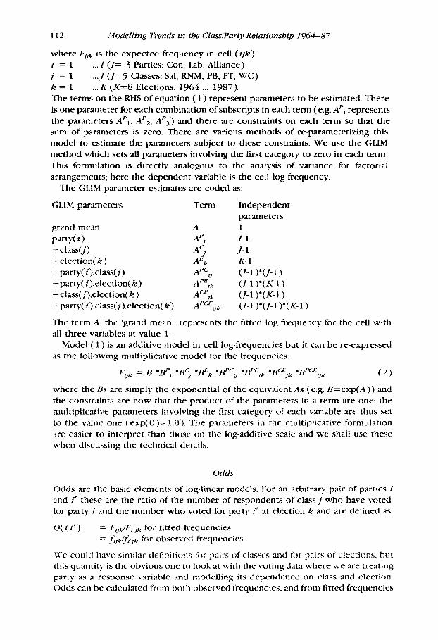
LogFiik = A + AP, + Aci + AfCi, + APE ik + ACEjk + A-,

where Fgk is the expected frequency in cell (& i = l... I (I=3 Parties: Con, Lab, Lib/Alliance) j = l... J (I= 5 Classes: Sal, RNM, PB, FT, WC) k= l... K (K=8 Elections: 1964, 1966, 1970, February 1974, October 1974, 1979, 1983, 1987). Since this model tits the data exactly, it implies that the association between party and class is different for each election. In terms of odds ratios the model implies that there is a different odds ratio for each party/class combination which differs for each election.3 The fitted odds ratios are identical to the observed odds ratios for each party/class/election combination.

The saturated model is not substantively interesting because it implies that there are no systematic underlying trends in the party/class association. Thus if we were to accept this model we would infer that there are no trends in the party/class relationship, simply that this relationship differs between elections. Of greater substantive interest are models which imply particular structures for the odds-ratios in the Table. So we shall now look at a series of relevant models for the analysis of trends in the relationship between class and party over elections.

The Base Model: No Trends

The first model we shall fit is the no trends model for all eight elections between 1964 and 1987. This model implies that the association between party and class does not vary with election. In other words, the odds ratios for each class/party combination are set to be constant across elections.

The model can be specified as follows:

LogVk = A + A’, + A’, + AL, + APC, + ApElk + ACE,,

These terms are interpreted as follows: the one-way terms ApI, AC, and AEk simply control for the numbers of respondents

106 Modelling Trends in the ClasslParty Relationship 1964-87

in the different categories of each variable. the term APC Ij says that party depends on (is associated with) class. the term APEik controls for variations in the votes of the parties over elections. the term AcEjk controls for the numbers in each class over elections (primarily, the increase in size of the salariat and the decrease in size of working class). Thus the no trends model is a baseline model which incorporates all of the one and two-way terms, thus controlling for changes in these variables, but does not include the three-way interaction between party, class and election (ApcEvk) which completes the saturated model.*

An inspection of the standardized residuals for the 120 cells show that in only two cells is the no trends model a significantly bad fit. Nevertheless, the model has a G2 of 84.75 with 56 degrees of freedom (p = 0.008) indicating that in terms of overall statistical significance the model does not fit well. We must therefore reject the hypothesis that there have been no changes in the class/party relation between elections. In other words, in order to fit the observed patterns in the data we need to examine the S-way term (APCEtik ). We shall now partition this term in ways which allow the testing of particular hypotheses about the form which the changes have taken. Consequently, in subsequent sections we consider models intermediate between the no trends and the saturated models.

Testing for Gradual Change: The Constant Trend Model

As described above, a key idea in recent discussions of class dealignment is that the solidarity and normative distinctiveness of the classes have declined, thus leading to a gradual decine in the links between classes and parties. We would expect such sociological changes to take a gradual but continuous form; Crewe for example talks of the ‘glacial character’ of social change. In order to test this theory of gradual change we shall fit a constant trend model of class dealignment.

The log-linear models considered so far treat all the variables defining the multiway table as nominal. Recently, a number of special log-linear models have been proposed for contingency tables where one or more of these variables is treated as ordered (Heath and Clifford, 1989; Agresti, 1984; Goodman, 1979). These models incorporate additional parameters which specify a systematic dependence of the associations between the nominal variables on the ordered variables. In the present context the variable election can be considered as an ordered variable, with party and class considered as nominal variables. We therefore propose the following model:

LogFi,, = A + A’, + A”, + AEk + Apt, + APElk + AcEjk + ApcvTk (3)

This is the no trends model with the extra term APC,Tk, Tk being scores assigned to the levels of the election variable. A natural scoring to use is the linear sequence: 0,1,2,3,4,5,6,7.

Like the saturated model, then, this model includes a three-way interaction between class, party and election. But unlike the saturated model it specifies a particular form to the interaction, namely a constant trend. Thus the odds ratios for each class/party combination are set to change at a constant rate.5 Consequently, since election is treated as a single ordered variable when it appears in the three- way interaction, fewer degrees of freedom are used. Thus whereas the three-way interaction uses 56 degrees of freedom in the saturated model, the form specified

GEOFFREV EVANS, ANTHONY HEATH AND CLWE PAYNE 107

in the constant trend model uses only 8 degrees of freedom. When fitted to our data, the constant trend model gives G* of 70.47 with 48df,

p = 0.02. This is still not a particularly good fit, and while it represents a reduction of 14.28 compared with the baseline no trends model, it uses up 8 degrees of freedom in securing this reduction (with a p-value of 0.06 for the change in G*).

This is not a significant reduction in G* and we cannot therefore conclude that the constant change model is a significant improvement over the no trends model.’

When examining the period from 1964 to 1987, therefore, neither the no trends nor constant trend model fits the data well. However, on inspecting the data of Table 2 it can be seen that the relation between class and party tended to be rather stronger in the 1964 and 1966 election surveys than it was in subsequent ones. This suggests that, in place of a constant trend, we might do well to fit a ‘once-for-all’ change in the class/party relation. We therefore score the eight elections as follows:

1,1,2,2,2,2,2,2 and we fit the following model:

Lo#~~ = A + APi + ACi + AEk + APCg + APE, + A”“i, + A”& (4)

where U, represents the new scoring of the election variable. The three-way interaction term uses up the same number of degrees of freedom as that in model (3) but of course specifies a different form to the relationship between class, party and election. This model sets the odds ratios for each election within each of the periods to the same level, but sets the odds ratios for each period to a different level.

Model (4) reduces G* to 60.22 with 48 df, p = 0.11. This represents a reasonably good fit to the data and supports the hypothesis that the relationship between class and party in the 1964 and 1966 surveys was different from that in the later periods. So we next fit a no trend model for all election surveys between 1970 and 1987 but excluding those in 1964 and 1966. This fits reasonably well too (G’ = 48.96, df 40, p = 0.16). (See also Marshall et al., 1988 for a similar analysis of the 1970- 85 period. )

Various interpretations of this finding are possible. First it may be the case that there were real ‘once-for-all’ sociological or political differences between the 1960s and the subsequent period. For example, the franchise was reduced to 18 in 1969, and it may be that young voters do not vote on class lines to the same extent that older voters do. Hypotheses of this form need to be specified and tested.

Alternatively, it may be that the election studies conducted in the 1960s differ procedurally horn the later studies, for example, there was a greater degree of clustering of the samples (only 80 sampling points being used compared with 250 in the 1983 and 1987 surveys). This would tend to produce larger design effects and hence larger confidence intervals. Once these design effects are taken into account, it may be that the difference between the 1960s results and the later ones will prove not to be statistically signiticant after all. In addition, data collection and coding procedures appear to be somewhat different, and it is perhaps worth noting that an alternative survey conducted at the same time showed a lower level of class voting in the 1960s than that reported in the two British Election Surveys (Miller, Tagg and Britto, 1986).

We could stop at this point, confident that there had been no trends in the class/ party relation since 1970 and uncertain how to regard the 1960s evidence. However, it is of some interest to explore further to see whether there are any alternative models which can account both for the 1960s and the subsequent

108 Modg~~~~g Tnmds in the ~~~S~Par~R~~a~~o~bi~ 1964-8?

results. We therefore turn to other ways to partition the three-way term to improve upon the fit of the baseline no trends model.

Partitioning the Three-way Interaction

Our response to this situation, therefore, is to change tack and try and understand the dynamics of class-vote relations in terms of political factors, rather than sociological trends. Thus, we have no formal need to treat election as an ordered variable. Instead we can conceive of this variable as being a proxy for some underlying political factors and then define ‘poiitical periods’, that is, combinations of elections, within which we hypothesize that the odds ratios for particular party/ class pairs are constant. For example, we can partition the three-way interaction term between party, class and election by fitting models in which we specify that some of the odds ratios for some party/class combinations vary with election.

Our guiding assumption is that classes may have different relations to political parties according to the policies adopted by the party when in office or espoused by them in election campaigns. In effect we are proposing that the strength of the class-party association may depend on whether the ‘class party’ ‘delivers the goods’ when in power or promises to promote class interests when next it comes to power.

Our first model of this type categorizes election according to the party that ‘won’. This model says that when a party wins an election it secures a different pattern of class support from when it loses. Thus inspecting Table 2, we can see that there was a higher level of class voting in 1964, 1966, February 1974 and October 1974 (elections which Labour may be said to have won) than there was in the other four elections. A possible interpretation of this is that the Labour party wins when it appeals to working-class interests but loses when it fails to do so. At any rate we fit the following model:

Log.Ftie = A + AP, + Aci + AE, + Ax9 + APEIg -t- A"";, + APc,V, (51

where V, is scored 1,1,2,1,1,2,2,2. Model (5) yields a G* of 66.35 with 48 degrees of freedom, p = 0.04. This is an

improvement on the constant trend model, but it still does not quite attain the minimum significance level of p = 0.05. An alternative model focuses on incumbency rather than on winning. That is to say, we postulate that it is the party’s record when in office which affects the pattern of its class support at the subsequent election. For this we propose the alternative scoring of the election variable, 1,1,2,1,1,2,1 ,I. Since the 1966 election followed hard on the heels of the 1964 election, and October 1974 followed even more closely on the February 1974 election, we have assumed that they did not really mark a new period of incumbency and we score 1966 and October 1974 to the same value as the immediately prior election.

We thus fit the following model:

LogFi,* = A + A", + A'; + AE, + APL‘, + APElk + ACE ]k + A’“,w, (6-I

This yields a CL of 63.59 with 48 degrees of freedom, p = 0.065. It is therefore a small improvement on model (5) and is within the p = 0.05 significance level.

As can be seen, models (5) and (6) give fits that are slightly better than that of the constant trend model (model 3) although inferior to that of the once-for-all change model (model 4). If we take the view that the I964 and 1966 data are

GEOFFREY EVANS, ANTHONY HEATH AND CLIVE PAYNE 109

unreliable and restrict ourselves to the 1970-87 period, the winners model and the incumbency model fare better, the former yielding a G2 of 37.01 with 32 degrees of freedom, p = 0.25, and the latter yielding a G* of 32.26 with 32 degrees of freedom, p = 0.45.

Both models would seem to provide useful ways of modelling the data for this period.’ However, only the incumbency model is a significant improvement over the no trends model for the 1970-87 period (reduction in G* = 16.7 for 8 df, p = 0.03). The incumbency model also fared better in the 1964-87 period. This suggests that the incumbency principle is a better way of understanding changes in the party/class relationship in the periods under consideration. Consequently, we shall consider this principle in more detail in our next set of models.

Further Partitioning of the Three-way Interaction

In addition to restoring the election variable in these ways, we can also restore the class or party variables in the three-way interaction term. There are of course very many possible ways of partitioning the three-way interaction, and we simply illustrate these possibilities with one example: we hypothesize that it is the relationship between the Labour party and the working class that changes between election periods, while the relationship between the other classes and the other parties fits a no trend model. We might argue, for example, that the failures of Wilson’s Labour administration in the 1960s and Callaghan’s administration in the 1970s particularly alienated the working class since they failed to ‘deliver the goods’ of full employment and raise standards of living. In contrast, it might be argued, the working-class has not punished Conservative failures since they did not in general have expectations of benefits from the Conservative party, while the Conservative party might have been rather more successful in securing benefits for their middle- class supporters.

We thus score the variables as follows:

Party 1 2 1 Con Lab All

C1a.S 111 1 2 SA RNMPB FT WC

Election 1 12 1 1211 64 66 70 74F 740 79 83 87

And we fit the following model:

Lo@~~ = A + AP, + Aci + AEk + APCg + APEjk + ACEjk + Z (7)

Where Z is defined below. /,PCE

fjk = Z if Class 0’) is 5 (working class) and Party (i) is 2 (Labour) and Election (k) is incumbent type 2 APCE

i/k = 0 otherwise This is the no trends model with the addition of one extra independent parameter.

Thus in this model all odds ratios for combinations involving Labour and the working class are constant within elections of a given incumbent type, but different between types. All other combinations of odds ratios for party/class/elections are set to a constant.

This model fits the data fairly well with G* of 67.84 on 55 df, p = 0.11. This is a

110 Modelling Trends in the Class/Party Relationship 1964-87

highly significant reduction of 16.9 in G* from the no trends model using only 1 df (p < O.OOl).” It indicates that Labour incumbency weakens the class/party association because it reduces the support of the working class for Labour. To illustrate this consider the odds ratio for (Labour/other:salariat/working class). At elections that do not follow a period when Labour has held offtce for some time this is 6.58. However, following Labour incumbency the ratio drops to only 4.51.

We next check the pattern using just the 1970s and 1980s elections. After all, if the effect is robust it should occur without using the data from the early and perhaps ‘suspect’ studies. As we have seen, fitting the no trends model for 1970-87 produced a G* of 48.96 with 40df. Fitting the incumbency model (with a Labour by working class interaction) reduced this to G* = 36.94 with 39df,p = 0.56. The reduction in G* from the no trends model is highly significant (p < 0.0001).9

Model (7) therefore, indicates that compared with other classes the working class has become relatively less supportive of Labour after periods of Labour government. This suggests that there is a special relationship between Labour and the working

class. Unfortunately for the party it is rather an unhealthy one: Labour government loses relatively more votes in the working class than elsewhere.

Interestingly, the 1987 election does not appear to fit this pattern. The relative support for Labour compared with other parties amongst the working class did not increase between 1983-87 (see Table 2)--a result not predicted by the incumbency principle. It could be suggested that the working class have become accustomed to Conservative government, with a corresponding decline in the

tendency to drift back to Labour after a period of Conservative government. Fitting model 7 for the 1964-83 period only, results in a G’ of 50.37 for 47

degrees of freedom (p = 0.34)-a good fit and an extremely impressive improvement on the fit obtained with the no trends model. Fitting the no trends model for the same period produces a G* of 72.65 for 48 df @ = 0.012). The reduction in G* obtained with model 7 is 22.28 for just 1 df (p < 0.0001).

It is therefore possible that the effects of Labour defence policy disputes have prevented their recapturing working class support during this particular period of Conservative incumbency. Certainly, there is evidence that compared with those in the salariat, working class Labour supporters are rather more critical of the party’s unilateralist policies (see Heath and Evans, 1988).

Of course, such an interpretation is rather ud hoc; there are many other possible partitionings of the three-way interaction term, and we do not wish to claim that we have found a unique ‘best model’ to fit the data. We are in any event rather suspicious of ‘data-dredging’ to find best-fitting models and prefer a hypothesis- driven approach-a unique best model which dominates all other possible models is unlikely to be found. Rather, to shed further light on the rival sociological and political accounts of the changing class/party relation we need to turn to additional data (such as attitudes to the incumbent government’s record), testing further inferences from the different theories. The aim of the modelling undertaken here is to provide the basis from which to develop such tests.

Conclusions

This paper contains only a brief summary of the analyses conducted, but the important points of the story are clear enough. The approach we have adopted has used suitable techniques to examine first, simple trends in the class-vote relation,

GE~FRW EVANS, ANTHONY HEATH AND CL~ PAYNE 111

and then more complex models related to substantive political hypotheses concerning the dynamics of class and party relations. In particular we have focused on the changing pattern of relations between those two old friends the Labour Party and the working class.

The finding that the attainment of government by the Labour Party has unfortunate consequences for its support in its ‘class heartland’ provides both an interesting discovery and an important question to be answered. It could be suggested that the best way for the working class to remain faithful to the Labour cause is for the party to keep on losing. However, the discovery that the third term of Thatcher government does not fit that pattern suggests that even that questionable ‘option’ may not be available to the party strategists.

Nevertheless, unlike observers who talk of secular, ‘sociological’ trends of a relatively irreversible nature, we do not wish to imply that the situation is not amenable to change by the Labour Party itself. By changing promises, policies, images and performance it is possible that a pattern that appears to have held for the 20 or so years between 1964-83 can be changed.

Finally, without wanting to diminish the importance of these interesting substantive implications of the modelling conducted here, we suggest that the two most important points to be taken from this paper concern the approach we have adopted to modelling patterns of political behaviour. On the issue of the techniques to be adopted when analysing trends in class/party relations, we have indicated the advantages of testing the fit of models by comparing their levels of statistical significance. This is clearly a more precise way of operationalizing our theories than is the more common approach of looking at coefficients of the class/party association for each election without testing for the statistical significance of changes in the relationships through time.

With regard to theory, we have given examples of the systematic application of theoretical principles concerning the dynamics of political relations between parties and classes. Obviously, there is much more work that can be done in refining the theories from which the three-way interaction term is partitioned. In this paper we prefer to remain agnostic on the particular form such refinements may take. However, we consider our findings do give a basis for further research into the relationship between social class and party that is not tied to a view of class-vote trends as gradual, sociologically determined changes in strengths of association. Instead, we suggest it could be profitable to investigate hypotheses that refer to political processes capable of generating complex and varied patterns of voting behaviour over relatively short periods of time.

Technical Appendices on Log-linear Models

Formal Definition of the Log-linear Model

The statistical package used to analyse the data is the Generalised Linear Interactive Modelling programme GLIM (Payne, 1985). In this appendix we use the standard notation for log-linear models.

We have a three-way party (P) by class (C) by election (E) table of observed frequencies, f+ The saturated log-linear model for this table is

LogFve = A + AP, + Acj + A”k + APC + APEik + ACE’ + APCEvk 1J # (1)

112 ~odei~ing Trends in the Chss/Purty Re~ut~onsbi~ 1364-87

where FO, is the expected frequency in cell (ijk) i=l . . . I (I= 3 Parties: Con, Lab, Alliance) j=l . . . J vi=5 Classes: Sal, RNM, PB, FT, WC) k=l . . . K (K=8 Elections: 1964 . . . 1987). The terms on the RHS of equation ( 1) represent parameters to be estimated. There is one parameter for each combination of subscripts in each term (e.g. A’, represents the parameters API, AP,, AP3) and there are constraints on each term so that the sum of parameters is zero. There are various methods of re-parameterizing this model to estimate the parameters subject to these constraints. We use the GLIM method which sets aII parameters involving the first category to zero in each term. This formulation is directly analogous to the analysis of variance for factorial arrangements; here the dependent variable is the cell log frequency.

The GLIM parameter estimates are coded as:

GLIM parameters Term independent parameters

grand mean A I

parv( i) AP, Z-l + class(J) AC, J-l 4 eIection( k) AEJZ K-l +party( i).classo) A PC

APE: (I-l)*u-l)

+party( i).election( k) (&l)*(K-1) + cIass~).eIection( k) ACE fk (Jl)*(K-1) +party( i).classG).eIection(k) AP6?

?I* (I-I)*cJ-l)*(K-1)

The term A, the ‘grand mean’, represents the fitted log frequency for the cell with all three variables at value I.

Model ( 1) is an additive model in cell log-frequencies but it can be reexpressed as the following multiplicative model for the frequencies:

F l/k = R *BP1 a@, *off *B’=cv *BPElk *@“Jk *@CEvk (2)

where the Bs are simply the exponential of the equivalent As (e.g. B=exp(A)) and the constraints are now that the product of the parameters in a term are one; the muitip~icative parameters involving the first category of each variable are thus set to the value one (exp(O)= 1 .O). The parameters in the muitiplicative formulation are easier to interpret than those on the log-additive scale and we shah use these when discussing the technical details.

Odds

Odds are the basic elements of log-linear models. For an arbitrary pair of parties i and i’ these are the ratio of the number of respondents of class j who have voted for party i and the number who voted for party i’ at election k and are defined as:

O(i,i’) = Fvk/Flill for fitted frequencies = J‘!,&>&. for observed frequencies

We could have similar definitions for pairs of classes and for pairs of riections. but this quantity is the obvious one to look at with the voting data where we are treating party as a response variable and modelling its dependence on class and election. Odds can be calculated from both observed frequencies. and from fitted frequencies

GEOFFREY EVANS, ANTHONY HEATH AND CLWE PAYNE

under a particular model.

113

Example: Observed odds for the salariat (j= 1) being Con rather than Iab (i= 1 rather than i=2) are 167/52 = 3.21 in the 1966 election (k=l). The same odds for the working class (j=5) are 175/469 = 0.37. Thus the observed odds of the salariat voting Con rather than Lab were 3.27:1; for the working class 0.37:l (or l/O.37 = 2.8:1 Lab rather than Con).

Odds Ratios for Class and Party

For an arbitrary pair of parties (i, i’ ) and an arbitrary pair of classes 0; j' ) we define the odds ratio for election k as:

This is the relative odds that class j vote for party i rather than party i’ at election k, compared with those for class j’. The odds ratio is a fundamental quantity in the analysis of contingency tables with log-linear models. It is a measure of the association between the two variables; a value of one corresponds to independence of the two variables. In this context we are interested in whether there are systematic trends in the degree of association between class and party over the levels of the third variable, election. Odds ratios can be formed for each of the I*(I- 1)/2 pairs of parties in combination with each of theJ*(I-1)/2 pairs of classes.

Each model fitted implies a statement about how the odds ratios vary systematically in the three-way table.

Example: The odds ratio for the salariat voting Con rather than Lab compared with the working class in 1964 are (167/52)/( 175/469) = 3.21//0.37 = 8.61. Thus the salariat were 8.61 times more likely to be Conservative than Labour than the working class in this election. This ratio for the 1987 election (k=8) is (467/130)/ (319/492) = 3.59/0.648 = 5.54.

Fitting the No Trends Model

In the case of the no trends model we set B I”cEijk to 1. Substituting equation (2) with BPCEok set to 1, in equation (3) we obtain

So this ratio does not vary with (is constant over) the levels of election (k). It simply depends on which combination of pairs of class and party is being considered.

The BPC r, parameters estimated (by GLIM for the term party.class) are:

Party (i) 1 -Con 2-Lab 3-Alliance

SA 1 1.00 1.00 1 .oo RNM 2 1 .oo 1.67 0.99

(j> PB 3 1 .oo 0.63 0.52 FT 4 1.00 3.17 1.09 WC 5 1.00 6.07 1.29

114 Modelling Trends in the ClasslParty Relationship 1964-87

Thus the odds ratio

BPC I I * Bpcas 1.0 * 6.07 P(Con,Lab:Sa, WC) = BPC * BPc,s = = 6.07

21 1.0 * 1.0

and takes this constant value for every election. This odds ratio will now be used to illustrate the consequences for particular odds ratios of different model specifications. Table 1 gives the observed and fitted odds and odds ratios for this combination of party/class. From these odds ratios we can see that there is a rapid decline in the relative odds in the early elections. But relative odds then increase again and are fairly constant except for drops in 1979 and 1987 when the two classes move closer together.

Appendix TABLE 1. Observed and fitted odds ratios for salariat/working class: Conservativekabour

Observed Fitted Sal WC Sal WC

K f, Iklf2,k f15k/f25k Rk F1lkm2lk FI5km25k Rk

167/52 175/469 3.21 0.37

170/69 1691500 2.46 0.34

178184 196f370 2.12 0.53

221/91 199/510 2.43 0.39

208/9 1 165/501 2.29 0.33

231/83 193/331 2.78 0.58

439/105 3411547 4.18 0.62

467/l 30 3191492 3 59 0.65

8.61

7.29

4.00

6.22

6.94

4.77

6.71

5.54

163/62 190/438 2.63 0.43

165/80 1671494 2.06 0.34

186/72 170/398

2.59 0.43 2 15/87 207/507

2.50 0.41 204/92 179/491

2.21 0.36 236/73 186/348

3.25 0.54 443/l 10 352/529

4.03 0.67 469/l 30 3071515

3.61 0.60

6.07

6.07

6.07

6.07

6.07

6.07

607

6.07

Fitting a Constant Trend

The constant trend model may be written as follows:

F r/k = B ‘BP. *Bc ‘BEk *Bpc,, I I *BpEik “BCE,, ‘ccliTk (5)

where Tk are scores assigned to the levels of the election variable in the linear sequence: 0, 1, 2, 3, 4, 5, 6, 7.

In GLIM this represents the additional term party.cZass.score with (I-1 )*u-1 ) = 8 extra parameters coded as party( i).class(j).score

where score = k-l for election k

RI’ for this model is obtained by substitution of (6) in (3) as

GEOFFIEY EVANS, ANTHONY HEATH AND CLIVE PAYNE 115

The parameter estimates for the calculation of the fitted odds ratios are: party( i).class(j) (Fii)

Party (9 1 -Con 2-Lab 3-Alliance

SA 1 1 .oo 1.00 1.00 RNM 2 1 .oo 1.65 1.17

(i) Ph 3 1 .oo 0.55 0.65 FT 4 1.00 3.62 1.04 WC 5 1.00 6.74 1.15

Party( i).class(j).score (cpcii)

Party (i) 1 -Con 2-Lab 3-Alliance

SA 1 1.02 1.05 1 .oo RNM 2 1.06 1.09 1 .oo

(i) PB 3 1.07 1.15 1.00 PT 4 1.01 1.01 1 .oo WC 5 1 .oo 1.00 1 .oo

[note GLIM sets parameters for last level of each variable to the value one here]

Thus the fitted odds ratio for (Con,Lab:Sa,Wc) at election 3

1.0 * 6.74 * = 1

1.0 * 1.0

= 6.74 * (0.97)*

Thus the first component is the overall fitted odds at election 1, the second component is a constant factor, 0.97, by which these odds are multiplied as we go from election to election. The Tk acts as a ‘power’ function for this factor with the power determined by which election it is in time sequence. The fitted values for this odds ratio show a constant, but small, relative decline as we move from election to election.

Thus we have R(1) = 6.74 R( 2) = 6.74 * (0.97) R(3) = 6.74 * (0.97)* R( 3) = 6.74 * (0.97)” etc

It may help the reader to compare the effects of the different models discussed so far on the odds ratios. In Table 2 the fitted odds ratios for Con,Lab:Sa,Wc are given for each of the models discussed in the Appendix. The calculation of the parameters and fitted odds for the other models discussed in the text is obtained in the same fashion as with the constant trend model, but using different scores for the election variate.

116 Modelling Trends in the CIasslParty Relationship 1964-87

1.

2.

3. 4.

5

6.

7.

x.

Appendix TARLE 2 Fitted odds ratios (Con,Lab:Sal,Wc) for various models

Election

Model 1 2 3

Observed No trend Constant trend

1964 8.61 6.07 6.74 1966 7.29 607 6.57 1970 4.00 6.07 6.39 1974F 6.22 6.07 6.22 19740 6.94 6.07 6.06 1979 4 77 6.07 590 1983 6.71 607 5.75 1987 5 54 607 5 59

Notes

The British General Election Studies are a series of representative probability samples

which have been conducted immediately following each general election starting in 1964.

The 1964, 1966 and 1970 election surveys were conducted by David Butler and Donald

Stokes at Nuffteld College, Oxford. The two 1974 surveys and the 1979 study were

conducted by Ivor Crewe and the British Election Studies team at the University of Essex.

The 1983 and 1987 surveys were directed by Heath. Jowell and Curtice and undertaken

by Social and Community Planning Research. The information in Table 1 is taken from

Table 3.1 in Heath, Jowell and Curtice, (1985, p.30), with the addition of data from the

1987 survey.

A formal definition of the log-linear model is given in the Appendix.

A discussion of odds, odds ratios and relative odds ratios is included in the Appendix.

Technical details of the model and examples of fitted odds ratios are given in the

Appendix.

Arguably the most desirable modei to use to test the hypothesis of class de-alignment is

one which specifies that the scaling factors change in the same direction, either

consistently down or up, but are not constrained to change at any particular rates. Odds

ratios which are initially greater than 1 should reduce monotonically; odds ratios initially

less than 1 should increase monotonically. tinfortunately, at present we cannot fit this

model directly in any standard statistical software system. It needs a special Fortran

program using numerical routines to maximize a non-linear function where sets of the

parameters are subject to inequality constraints. Because of the considerable difficulties involved in such a project we shall address the issue of monotonic trends in a later paper.

The scoring used above implies an equal spacing of elections If we instead use the scoring

w’& = number of days (months) since the 1964 election, so that the scoring represents

‘real time’ there is hardly any difference in the fit of this model (G’ = 69.62, df = +8, p- value = 0.022), and the reduction in G2 ( 15.13 for 8 df) is not significant at p = 0.05.

Fitting a constant trend to the 1970-87 period resulted in a somewhat worse fit (CL of

39.73 with 32 degrees of freedom, p = 0.16-a non-significant reduction in CL from the no trends model)

We also fitted this model with foremen and techniclam coded a5 2. thus includmg them

with the workmg class. Interestingly the fit was far worse, supplying further evidence of

the importance of distinguishing between the two categories of manual work when

looking at class/party relations.

GEOFFREY EVANS, ANTHONY HEATH AND CLIVE PAYNE 117

9. There was some concern about whether the significance of the effect of the working class may be a result of the larger size of that class making a close fit to the observed data less likely. We therefore checked to see if the significance of other classes increases when they are aggregated to roughly the same size as the working class. However; the relationship between the other classes and particular parties remained insignificant, indicating that the findings are not artefacts of variations in the size of the classes.

References

A. Agresti, Analysis of Ordinal categorical Data, (New York: Wiley, 1984). J. Aldrich and F. Nelson, Linear Probability Logit, and Probit Models, (Beverley Hills, Sage,

1984). D.F. Alwin, ‘Measurement and the interpretation of effects in structural equation models’, in

J. Scott Long, Common Problems/Proper Solutions: Avoiding Error in Quantitative Research, (Beverley Hills, Sage, 1988).

R. Breen, ‘Fitting Nonhierarchical and Association Models using GLIM’, Social Methods and Research, 13: 1984, pp. 77-107.

D.E. Butler and D. Stokes, Political Change in Britain (revised edition), (London: Macmillan, 1974).

D. Cox, The Analysis of Binary Data, (London: Methuen, 1970). I. Crewe, B. Sarlvik and J. Ah, ‘Partisan dealignment in Britain, 1964-74’ British Journal of

Political Science, 7: 1977, pp. 129-90. M. Franklin, The Decline of Class Voting in Britain, (Oxford: Clarendon Press, 1985). L. Goodman, ‘Simple Models for the Analysis of Association in Cross-Classifications Having

Ordered Categories’, Journal of the American Statistical Asociation, 74: 1979, pp. 537- 52.

A.F. Heath and P. Clifford, ‘Class inequalities in education in the twentieth century’, Journal of the Royal Statistical Society, series A, 1989.

A.F. Heath and G. Evans, ‘Working class conservatives and middle class socialists’, in R. Jowell et al. (editors), British Social Attitudes: the 5th Report, (Aldershot: Gower, 1988).

A.F. Heath, R. Jowell and J. Curtice, How Britain Votes, (Oxford: Pergamon, 1985). A.F. Heath, R. Jowell, J. Curtice, G.A. Evans, J. Field and S. Witherspoon, Understanding

Political Change, (Oxford: Pergamon, 199 1). D. Hibbs, ‘Economic outcomes and political support for British governments among

occupational classes: a dynamic analysis’, American Political Science Review, 76: 1982, pp. 259-79.

S.M. Lipset, Political Man, (Garden City, New York: Doubleday, 1960). G. Marshail, D. Rose, H. Newby and C. VogIer, Social Class in Modern Britain, (London:

Hutchinson, 1988). W L. Miller, S. Tagg and K. Britto, ‘Partisanship and Parry Preference in Government and

Opposition: The Mid-term Perspective’, Electoral Studies, 5: 1986, pp. 3 l-46. C. Payne, The GLIM system, release 3.77 manual, (Oxford: NAG, 1985). A. Przeworski and K Sprague, Paper Stones: A History of Electoral Socialism (Chicago:

University of Chicago Press, 1986). P. Pulzer, Political Representation and Elections in Britain, (London: Allen & Unwin, 1968). R. Rose and 1. McAllister, Voters Begin to Choose: From Closed Class to Open Elections in

Britain, (London: Sage, 1986).