e

SVENSK KÄRNBRÄNSLEHANTERING AB

SWEDISH NUCLEAR FUEL

AND WASTE MANAGEMENT CO

Box 3091, SE-169 03 Solna

Phone +46 8 459 84 00

skb.se

SVENSK KÄRNBRÄNSLEHANTERING

Modelling the hydraulic interaction between engineered and natural barriers

Task 8 of SKB Task Forces GWFTS and EBS

Veli-Matti Pulkkanen

P-1

7-0

5M

od

ellin

g th

e h

ydrau

lic in

terac

tion

be

twe

en

en

gin

ee

red

and

natu

ral barrie

rs– Task 8

of S

KB

Task Forc

es G

WFT

S an

d E

BS

Report

P-17-05June 2017

Modelling the hydraulic interaction between engineered and natural barriers

Task 8 of SKB Task Forces GWFTS and EBS

Veli-Matti Pulkkanen VTT Technical Research Centre of Finland Ltd

ISSN 1651-4416SKB P-17-05ID 1588113

June 2017

This report concerns a study which was conducted for Svensk Kärnbränslehantering AB (SKB). The conclusions and viewpoints presented in the report are those of the author. SKB may draw modified conclusions, based on additional literature sources and/or expert opinions.

Data in SKB’s database can be changed for different reasons. Minor changes in SKB’s database will not necessarily result in a revised report. Data revisions may also be presented as supplements, available at www.skb.se.

A pdf version of this document can be downloaded from www.skb.se.

© 2017 Svensk Kärnbränslehantering AB

SKB P-17-05 3

Executive summary

This report summarizes the work carried out at VTT Technical Research Centre of Finland Ltd for Posiva Oy to model the hydraulic interaction between the water unsaturated bentonite buffer and the bedrock in Bentonite-Rock Interaction Experiment (BRIE) conducted in Äspö Hard Rock Laboratory. The modelling has been performed in the context of Task 8 by SKB Task Force on Groundwater Flow and Transport of Solutes.

The general objective of Task 8 is to increase the understanding of the hydraulic interaction between the partially water saturated bentonite and the rock to enhance the ability to model such interaction. The objective is aimed at by carrying out a series of efforts to model the wetting of bentonite in BRIE, namely subtasks a–d and f. In these subtasks, the complexity of the models and the amount of available experimental data gradually increases. Within this frame, the specific goal of the modelling described in this report was to build a relatively simple model that still captures the most important features affecting the interaction of the bentonite and the bedrock. The general objective can be met by analyzing the simulated results with respect the experimental results obtained from BRIE.

The specific goal of this work is achieved by joining a simple van Genuchten type of wetting model for bentonite to a bedrock hydraulic model concept that combines 1) discrete water conducting features mostly near the bentonite-bedrock interface on experimentally determined locations, 2) rock described by the concept of equivalent porous medium and 3) a simple wetting model for bedrock. The approach allows the inclusion of detailed geometrical features to the model where they are needed, but still the model can be calibrated with a somewhat small amount of experimental data and the model is not excessively heavy computationally. The concept also allows a mechanical coupling of the bedrock to the hydraulic model.

Whereas the first two subtasks, a and b, are treated as model developments exercises, the subtask c gives the first meaningful bentonite wetting time estimates ranging from 10 months to 50 years for a compacted bentonite cylinder with 30 cm diameter and around 3 meters height placed in bedrock. According to the simulations, the hydraulic conductivity of the intact bedrock near the bentonite filled borehole is the most important factor affecting the wetting time. Only when the hydraulic conductivity of this rock mass is low, the fractures and other well water conducting bedrock features begin to affect the wetting time. Otherwise, the simulations indicate that bentonite wets through the rock mass in approximately 10 months.

In subtask d, the available experimental data set is wider than in subtask c, but still the uncertainties related to the intact rock mass hydraulic conductivity prevent giving reliable wetting time estimates for bentonite. The mechanically coupled bedrock hydraulic model gives insight into the flow paths in the bedrock, but the effect on the wetting of bentonite is limited, unless the stress changes in bedrock open new pathways for groundwater flow. With the full experimental data set from BRIE in subtask f, the wetting time for bentonite in a borehole with a long dry section specifies to around 40 years and for bentonite in a borehole with water sources throughout the height of it to less than 10 years. Especially the hydraulic conductivity values for the intact rock and the relative humidity sensor data from BRIE give means to make the wetting time estimates to converge to the specific values. Although the simulation results can be used to estimate the wetting of bentonite, a comparison between the modelled and experimental relative humidity profiles through the bentonite – intact rock interface reveal that the wetting model concepts should be carefully revisited.

4 SKB P-17-05

Sammanfattning

Denna rapport sammanfattar det arbete som utförts vid VTT Technical Research Centre of Finland Ltd på uppdrag av Posiva Oy. Uppdraget innefattar att modellera den hydrauliska interaktionen mellan den med avseende på vatten omättade bentonitbufferten och det omgivande berget i försöket Bentonite-Rock Interaction Experiment (BRIE) som genomfördes vid Äspö Hard Rock Laboratory. Modelleringen har utförts inom ramen för Task 8 inom SKB Task Force on Groundwater Flow and Transport of Solutes.

Det generella syftet med Task 8 är att öka förståelsen för den hydrauliska interaktionen mellan den delvis vattenmättade bentoniten och berget för att förbättra förmågan att modellera en sådan interak-tion. Målet syftar till att genomföra en rad uppgifter för att modellera vattenupptag av bentonit i BRIE, nämligen modelleringsuppgifterna 8a-d och f. I dessa modelleringsuppgifter ökar komplexiteten hos modellerna och mängden tillgängliga experimentella data gradvis. Inom ramen för Task 8 var det specifika målet för modelleringen, som beskrivs i denna rapport, att bygga en relativt enkel modell som fortfarande fångar upp de viktigaste dragen som påverkar samspelet mellan bentoniten och berget. Det generella målet uppfylls genom att analysera de simulerade resultaten med hänsyn till de experi-mentella resultaten som erhållits från BRIE.

Det specifika målet för detta arbete uppnåddes genom att man inkluderade en enkel bevätnings-modell för bentonit av van Genuchten-typ i ett hydrauliskt grundvattenmodelleringskoncept som kombinerar 1) diskreta vattenledande sprickor som mestadels ligger nära gränssnittet mellan bentonit och berg på experimentellt bestämda platser, 2) berget beskrivs som ett ekvivalent poröst medium och 3) en enkel vätningsmodell för berget. Tillvägagångssättet möjliggör införande av detaljerade geometriska egenskaper i modellen där de behövs. Modellen kan fortfarande kalibreras med en viss, men förhållandevis liten mängd experimentella data. Dessutom är inte modellen överdrivet stor beräkningsmässigt sett. Konceptet möjliggör också en mekanisk koppling av berget till den hydrauliska modellen.

Emedan de två första delarna, a och b, av Task 8 behandlades som modellutvecklingsövningar, gav deluppgift c de första meningsfulla bentonitvätningstiderna från 10 månader till 50 år för en komprimerad bentonitcylinder med en diameter på 30 cm och en höjd av ca 3 meter placerad i ett hål i berget.

Enligt simuleringarna är det intakta bergets hydrauliska konduktivitet nära det bentonitfyllda borrhålet den viktigaste faktorn som påverkar vätningstiden. Först när bergmassans hydrauliska lednings-förmåga är låg, börjar sprickorna och andra vattenledande objekt i berget påverka vätningstiden. I annat fall indikerar simuleringarna att bentonit väts genom bergmassan inom cirka 10 månader.

I deluppgift d av Task 8 är omfattning av den tillgängliga mängden experimentella data större än den i deluppgift c, men fortfarande försvårar osäkerheterna kopplade till den hydrauliska konduktiviteten för intakt bergmassa möjligheten att erhålla tillförlitliga uppskattningar av vätningstid för bentonit. Den mekaniskt kopplade hydrauliska bergmodellen ger insikter om flödesvägarna i berget, men effekten på vätningen av bentonit är begränsad, såvida inte bergspänningen förändras så att nya vägar för grundvattenflödet öppnas. Den fullständiga experimentella datamängden från BRIE i deluppgift f anger vätningstiden för bentonit i ett borrhål med en lång torr sektion till cirka 40 år och för bentonit i ett borrhål med vattenkällor över hela dess längd till mindre än 10 år. Speciellt de hydrauliska konduktivitetsvärdena för det intakta berget och relativ fuktighetsdata från sensorerna i BRIE möjliggjorde att uppskattningarna av vätningstiderna konvergerande till specifika värden. Även om simuleringsresultaten kan användas för att uppskatta vätningen av bentonit, visar en jäm-förelse mellan de modellerade och experimentella relativa fuktighetsprofilerna genom gränssnittet mellan bentonit och det intakta berget att vätningsmodellkoncepten bör kontrolleras och studeras noggrant.

SKB P-17-05 5

Preface

Äspö Task Force on Groundwater Flow and Transport of Solutes began to work on Task 8 in around 2010 and the year when writing this report is now 2016. During this time not only the name of the Task Force has evolved to SKB Task Force on Groundwater Flow and Transport of Solutes but also the people working in the project at VTT have changed in time. The work was initiated by prof. Markus Olin and Aku Itälä. Aku carried out the TOUGH2 simulations in subtask 8a and was involved in the modelling work until the subtask b. That was about the time when I, Veli-Matti Pulkkanen, was introduced into the project. Later on, during subtask d, Karita Kajanto wrote her Master’s Thesis on the mechanically coupled hydraulic model for fractured rock in a project related to VTT’s Task 8 project. The mechanically coupled bedrock hydraulic model in subtask d bases on her work. The rest of the model development and the simulations have been conducted by me. I am also the writer of this report and hope that I managed to summarize the work by the previously mentioned people at least with some clarity and without too many mistakes.

SKB P-17-05 7

Contents

1 Introduction 91.1 Background 91.2 Objectives 91.3 Scope 10

2 Task 8a – Getting started 112.1 Objectives 112.2 Approach 112.3 Model setup 112.4 Results 122.5 Discussion 152.6 Conclusions and recommendations 15

3 Task 8b – From two dimensions to three 173.1 Objectives 173.2 Approach 173.3 Model setup 183.4 Results 183.5 Discussion 193.6 Conclusions and recommendations 19

4 Task 8c – Blind predictions for the wetting time of BRIE with discrete fractures 21

4.1 Objectives 214.2 Approach 214.3 Model setup 214.4 Hydraulic model calibration 234.5 Results 254.6 Discussion 304.7 Conclusions and recommendations 32

5 Task 8d – Coupling the hydraulic model to rock mechanics and adding geometrical details 33

5.1 Objectives 335.2 Approach 335.3 Mechanically coupled hydraulic models at the testing stage 35

5.3.1 Fracture models 355.3.2 Bedrock matrix models 36

5.4 Model setup at the testing stage 375.5 Model calibration at the testing stage 385.6 Results of the testing stage 385.7 Choosing the mechanically coupled hydraulic model for the wetting model 455.8 Wetting model setup 465.9 Wetting model calibration 475.10 Wetting model results 485.11 Discussion 555.12 Conclusions and Recommendations 57

6 Task 8f – back analysis with full data 596.1 Objectives 596.2 Approach 59

6.2.1 The evolution of the model: Simulations 596.3 Model setup 616.4 Model calibration 626.5 Results 63

6.5.1 Comparing the simulations with and without the pegmatite 63

8 SKB P-17-05

6.5.2 Comparison of simulations with different hydraulic conductivities for the low permeable zone 63

6.5.3 Comparison of different wetting models for the bedrock 636.5.4 Results from the final simulation 65

6.6 Discussion 716.6.1 Wetting characteristics of bentonite in the final simulation 716.6.2 The effect of the pegmatite vein 716.6.3 The effect of the hydraulic conductivity of the low permeable zone 726.6.4 The wetting models 726.6.5 Water conducting features at the rock-bentonite interface 736.6.6 Model concept: Geometry 746.6.7 Rock mechanical effects 756.6.8 The effects of deformation and stress of bentonite during wetting 766.6.9 Estimation of the total wetting time 77

6.7 Conclusions and recommendations 77

7 Concluding summary 79

8 References 81

Appendix A The wetting and flow model equations 83

Appendix B Initial values and boundary conditions 87

Appendix C Model parameters 91

Appendix D Task 8a pressure profiles 93

Appendix E Task 8b pressure and saturation profiles 97

Appendix F Comparing the wetting model to the water uptake test 99

SKB P-17-05 9

1 Introduction

1.1 BackgroundTask 8 is a joint effort of SKB Task Force on Modelling of Groundwater Flow and Transport of Solutes (GWFTS) and SKB Task Force on Engineered Barrier Systems (EBS) focusing on the hydraulic interaction between the bentonite buffer and bedrock in geological disposal systems for spent nuclear fuel. The task consists of the bentonite rock interaction experiment (BRIE) done at Äspö Hard Rock Laboratory (HRL) and of the effort by modelling teams to model the experiment.

The geological disposal concept KBS-3 originating from Sweden is followed also in Finland. According to the concept, sets of fuel bundles are sealed into copper canisters with cast iron inserts. The canisters are surrounded by bentonite buffers to provide them a stable chemical environment and to protect them mechanically. The whole packages are placed into boreholes drilled in tunnel floors in the depth of approximately 400 meters in Finnish bedrock.

Since the bentonite buffers and the bedrock act as barriers for isolating the spent fuel from the surface environment, both the bentonite as a buffer material and the bedrock at the Finnish disposal site are under thorough investigations. The two barriers, however, are studied by different groups of people and the interaction between the barriers has not been in the focus of the investigations. Therefore, Task 8 and BRIE having a KBS-3 relevant experimental setup are of direct interest of Posiva, for which VTT Technical Research Centre of Finland works as a consultant.

VTT has a history of performing research on nuclear waste management related topics such as radio-nuclide transport calculations and safety analysis, groundwater flow modelling and bentonite. The emphasis for VTT and Posiva in Task 8 is to combine the needed features of bentonite wetting and groundwater flow modelling to a new, relatively simple model concentrating on the bentonite-rock interface.

1.2 ObjectivesAccording Task 8 description (Vidstrand et al. 2017), ‘the overall objective of Task 8 is to enhance the understanding and increase our ability to model the hydraulic interaction between the rock and water unsaturated bentonite on both the scale of an individual deposition hole scale as well as the scale of a deposition tunnel. As an end result, the task is expected to deliver suggestions for better methods to choose deposition hole positions and hence a better predictability of interactions among deposition holes that are still empty and deposition holes that filled with bentonite and contain storage canisters.’

In Task 8, GWFTS and EBS task forces are intended to collaborate to produce a better understanding for the interaction between the bentonite buffer and bedrock. The task is not, however, intended to produce complex coupled models of the system meaning that the conceptual basis for the models for unsaturated bentonite and bedrock is in van Genuchten type of retention.

The objectives and the models used vary between the modelling teams depending on their specific interests, background and expertise. VTT’s objective is to use the models and data made available by the technical committee of Task 8 effectively to produce estimates of the wetting behaviour of the BRIE experiment in a way that might be useful when estimating the behaviour of the final disposal system. Wetting models not being developed or modified in this work, the modelling relies on the validity of the technical committee’s recommended conceptual models and on the quality of the data. The approach also means that the uncertainties in the positions, sizes and transmissivities of the bedrock fractures not observed directly are not tried to be captured with stochastic fracture network modelling but with simple deterministic models, since the stochastic option would require a large number of heavy wetting simulation runs in order to obtain meaningful mean values for the results.

10 SKB P-17-05

1.3 ScopeThis report covers the modelling in and results of the five subtasks a, b, c, d and f. The general outline follows the subtasks, but the model details, such as equations and parameters, can be found in the appendices.

Subtasks a and b were treated as model development and testing exercises, not as final modelling effort with accurate results. In these subtasks, the evaluation of the capabilities of different programs suitable for the modelling Task 8 and getting acquainted with the software are the major themes, whereas the wetting models and parameters were kept as they were suggested in Task 8 description (Vidstrand et al. 2017). In subtask 8a, the wetting of bentonite in a cylinder symmetric geometry including bedrock and a tunnel section were modelled with two simulation programs, namely COMSOL Multiphysics and TOUGH2 with PetraSim GUI. In subtask 8b, the wetting of bentonite in a three dimensional geometry (close to the BRIE geometry) was modelled using COMSOL Multi physics. Bedrock and the fractures were considered as equivalent porous media in the models.

In subtask c, the wetting time of bentonite in BRIE experiment (borehole 17 only) was predicted using the observed inflow values for the borehole cutting fractures. The data was limited such that it mimicked the data possibly available of a real final disposal system and this restriction was followed closely. A new feature in the model if compared to subtask 8b model was the inclusion of small borehole cutting fractures and large deterministic features as discrete fractures. The wetting models for bentonite and bedrock were kept as given in the task description, but a number of combinations of the bulk bedrock hydraulic conductivity, small fracture transmissivities and boundary conditions giving the same observed inflow values were tested to scope the wetting time of BRIE.

More detailed data was available in subtask d than in subtask c. Most importantly, the inflow values into the BRIE tunnel section and the more precise positions of the fractures gave restrictions for the model parameters and setup. The nappy test data on the inflow values into and pattern of borehole 17 gave insight in the bentonite rock interface: the most of the water flows into the borehole through the fracture, but there is also possible flow through a pegmatite vein and the borehole walls. Moreover, a rock mechanical model coupled to a water flow model developed in a side project of VTT’s Task 8 project was used as the hydraulic model in the subtask. Similarly to the previous subtask, the borehole 17 was concentrated on in the modelling.

A back-analysis of BRIE was conducted in subtask f. The results obtained by dismantling BRIE were the basis for the modelling effort. Although the new experimental results give much new insight how to re-conceptualize the bedrock-bentonite interface in a model, no new model development is carried out in the subtask. The idea is rather to evaluate the performance of the previous subtasks’ model with the final data than begin new effort to capture the details of BRIE. Therefore, the subtask 8d model (without mechanical coupling) is updated to serve as the model for subtask f by correcting the fracture positions and re-parametrising the hydraulic model for the bedrock (including borehole cutting pegmatite vein and fractures, large fractures, a low water permeable zone around the boreholes and bulk, or equivalent porous medium, bedrock). Besides the modelling, discussing the features of the model in relation to the final experimental results is focused in the subtask.

SKB P-17-05 11

2 Task 8a – Getting started

2.1 ObjectivesThe objective was simply to set up van Genucthen type of bentonite wetting models with COMSOL Multiphysics and TOUGH2 (PetraSim GUI and EOS9) in a two dimensional axisymmetric geometry to get rough estimates of the wetting time and to evaluate the performance and applicability of the software on this type of problem.

2.2 ApproachThe wetting of a cylindrical bentonite block in a borehole in a fairly simple axisymmetric geometry (bedrock and fractures as equivalent porous media) was modelled with a two-step approach. Firstly, a stationary pressure field in a bedrock block was computed assuming there is no bentonite in the borehole (air-pressure, 0.1 MPa, boundary condition). Secondly, having the stationary pressure field as an initial value, the wetting of bentonite was calculated time-dependently using the van Genuchten type of unsaturated flow equations as extension to the Darcy type of flow equation. The relative permeability in the COMSOL Multiphysics model was the cubic law, whereas the van Genuchten relative permeability was used with TOUGH2. The capillary pressure curve for both the models was the same van Genuchten type of curve (see Appendices A, B and C for the equations and the parameters). The approaches by two programs to solve the equations differ slightly.

2.3 Model setupThe axisymmetric, two-dimensional model geometry contains bentonite in a borehole (depth 3 m, radius 15 cm) on the tunnel floor (see Figure 2-1). The tunnel is surrounded by bedrock extending approximately 20 metres around the tunnel. A fracture cutting the hole at the middle point is included as a slice of bedrock (height 10 cm) which conducts water better than the surrounding bedrock. As the fracture, the intact bedrock is also handled as equivalent porous medium where the effect of fractures is included in the hydraulic conductivity.

Figure 2-1. The cross-sections of the cylindrical model geometry. The highly water conducting zone (height 10 cm) on the mid-height of the bentonite cylinder mimics a fracture. The pictures are from Vidstrand et al. (2017).

12 SKB P-17-05

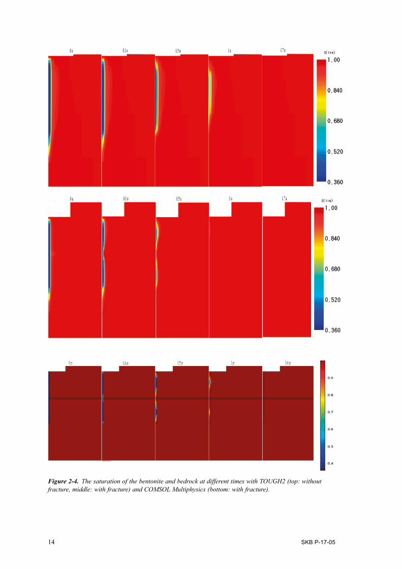
2.4 ResultsThe models were solved with and without a fracture and the results are presented in the figures below and in Appendix D. The TOUGH2 model reaches full saturation in 1.7 years in the case without the fracture and in 1.1 years with the fracture. The corresponding times with COMSOL model are 2.4 and 1.6 years.

Figure 2-2. Pressure fields with TOUGH2 at different times in the case without the fracture (top) and with the fracture (bottom).

SKB P-17-05 13

Figure 2-3. Close-up plots of the pressure fields near the bentonite with TOUGH2 at different times in the case without the fracture (top) and with the fracture (bottom). The pressures below the limit of the legends are marked with the colour of the limit value.

14 SKB P-17-05

Figure 2-4. The saturation of the bentonite and bedrock at different times with TOUGH2 (top: without fracture, middle: with fracture) and COMSOL Multiphysics (bottom: with fracture).

SKB P-17-05 15

2.5 DiscussionThe results with TOUGH2 and COMSOL Multiphysics differ somewhat, but the experience gained using the programs and getting idea of the quantitative behaviour of the system are more important than the exact results at this point. The differences were probably caused by the fact that van Genuchten relative permeability is used for bentonite with TOUGH2 (the standard option), whereas the relative permeability was modified to the cubic power law in COMSOL. Also, the grid size with TOUGH2 (total of 2 886 control volumes for the whole model, COMSOL: 20 000 degrees of freedom) is relatively low if contrasted to the nonlinearity of the retention curves for bentonite and bedrock.

A particular observation from the results is the drying of the bedrock near the bentonite when the saturation begins. This is due to the retention model parameterisation: the saturation of bentonite remains high (tens of per cents) even with high suction values (>100 MPa), whereas the saturation of bedrock is practically zero with these values. Another observation is that the pressure levels further than approximately 5 metres from the bentonite do not change very much with time (see the COMSOL graphs in Appendix C).

The saturation times of the models without and with the fracture should not be compared directly, since they do not correspond to each other in a real system. Adding a highly water conducting zone into the bedrock obviously shortens the wetting time. In a real system, however, the inflow into the borehole would be the measured value. Therefore, the permeability of the intact bedrock should be lowered to compensate the high permeable fracture zone to make the fracture and no fracture cases comparable.

The two programs solve the wetting problem with different approaches. TOUGH2 solves the pressure in the saturated parameter field and the saturation in the unsaturated field meaning that the program changes variables whenever saturated-unsaturated limit is crossed. In contrast, COMSOL Multi-physics model solves the pressure in both unsaturated and saturated parameter field. These two approaches result in different ways to handle the interface, where the van Genuchten-type of wetting models are not well defined. When solving only the pressure, the multiplier in front of the time derivative of the pressure has to be made continuous (see Equations A-8 and A-13) at the interface if symbolic derivation is used (COMSOL does it). This can be done by extending the saturated zone multiplier (the specific storage coefficient) to the unsaturated zone by multiplying it by saturation (see Equation A-14). This procedure does not affect the solution much if the storage term is not too large (about < 1 × 10−9 1/Pa). When solving the saturation in the unsaturated zone, the discontinuity problem moves to the saturation derivative of the pressure (∂p/∂S), which tends to infinity when satura-tion tends to one. To avoid the problem, TOUGH2 jumps over the transition region (1 × 10−6 < S < 1) when changing the variables from pressure to saturation (or vice versa, see Pruess et al. 2012). The program also uses numeric derivation which makes the problem less severe.

2.6 Conclusions and recommendationsBoth TOUGH2 with PetraSim GUI and COMSOL Multiphysics were used to solve the wetting problem. COMSOL, however, offers more flexible ways to handle equations and geometries (especially three dimensional ones and CAD files) and includes more efficient solvers (parallelism etc.) than TOUGH2. Therefore, it was chosen to be the program to be used in the following subtasks.

Special care should be taken of the bentonite-bedrock interface when meshing, because of the possible drying of bedrock.

A couple tens of meters of bedrock surrounding the tunnel section and the bentonite block should be enough for the models, since pressure levels further did not change much with time in the model here.

The wetting time estimates are around two years which is a prediction of the time that BRIE should take.

SKB P-17-05 17

3 Task 8b – From two dimensions to three

3.1 ObjectivesTask 8b was considered as a proof-of-modelling-concept type of exercise. The goal was to find out whether it is feasible to model the wetting of bentonite and groundwater flow in a three dimensional geometry where geometric scale differences are large. Special problems were importing the features in a CAD file into the model and the inclusion of fractures in COMSOL Multiphysics, which is designed to include three dimensional geometry objects in three dimensional geometries. In other words, one objective of the subtask was to get familiar with the modelling problems that should be solved in order to develop a detailed geometric features including model for BRIE.

The objective regarding BRIE was to test the effect of the fracture location on the wetting time.

3.2 ApproachThe wetting of a bentonite cylinder in BRIE tunnel geometry from Äspö HRL (see Figure 3-1 and Figure 3-2) was modelled. The bedrock and the fracture were treated as equivalent porous media, but testing the methods to implement discrete fractures was also started.

Two-step approach similar to the one in subtask 8a was used in the model. Firstly, the stationary pressure field was computed assuming the borehole walls open. Then, the pressure field set the initial pressure for the bentonite wetting computation. The same equations for Darcy type of flow and van Genuchten type of wetting as in subtask 8a COMSOL computations were used (see Appendices A, B and C for the equations, parameters and boundary conditions).

COMSOL Multiphysics can be utilized roughly in two ways. Either the pre-implemented modules for problems in different fields of physics can be used as they are, or the partial differential equations can be written directly to solve them with solvers in COMSOL. The first approach was chosen in this subtask. The only modification to the Earth Science modules Richards’ equation was the replacement of the van Genuchten relative permeability by the cubic law for bentonite.

Figure 3-1. Äspö HRL tunnel geometry around the BRIE experiment (in the boxed area) and computed pressure field (Äspömodel05 with DarcyTools v3.3). The CAD geometry of the same cubic bedrock block is on the right hand side. Figures are from Vidstrand et al. (2017).

18 SKB P-17-05

Figure 3-2. The model geometry. 40 m × 40 m × 40 m cubic bedrock block includes tunnels and a bentonite filled borehole. Fractures cutting the borehole are presented as 10 cm high horizontal bedrock zones that conduct water better than the bedrock around them.

Bentonite filled borehole (height 3 m, Ø=30 cm)

3.3 Model setupThe model geometry consists of a 40 m × 40 m × 40 m cubic bedrock block including a tunnel section and a bentonite filled borehole (see Figure 3-2). Three locations for the fracture (three dimensional high permeable zones with height of 10 cm) were tested: 0.75, 1.5 and 2.25 metres below the tunnel floor. The fractures cut the whole bedrock block horizontally. The solved equations, parameters and boundary conditions can be found in Appendices A, B and C.

3.4 ResultsThe wetting times for the cases with different fracture location are shown in Table 3-1. The wetting is visualized in Figure 3-3and Figure 3-4 below and the figures in Appendix D.

Table 3-1. The wetting times with diffenrent fracture locations. The total wetting times (saturation = 1) are at the middle column and the wetting times of the horizontal plane at the 1.5 m depth from the tunnel floor are on the rightmost column.

Distance from tunnel floor (m) Wetting time (years) Wetting time of plane at 1.5 m (years)

0.75 1.3 1.21.5 1.5 0.72.25 1.8 1.2

SKB P-17-05 19

3.5 DiscussionThe results show that wetting of bentonite and water flow in bedrock can be modelled in a same COMSOL Multiphysics model. To have a model to predict the wetting of BRIE, however, requires a bulk of model development. A flexible way to include fractures with different orientation is needed to incorporate observed features into the model. Also, the constant hydraulic conductivity of bedrock could be replaced with a more delicate bedrock model that takes advantage of the available fractures statistics, or that is related to the bedrock stress. In addition, improvements, for example, to the mesh density has to be made (see Figure 3-3).

This subtask served mostly as a model development exercise and the results concerning the behaviour of BRIE should be regarded with caution. Nonetheless, the wetting time prediction is the shortest with the upper most fracture and longest with the lowest fracture position. The effect of the fractures is still relatively small, since bentonite wets through the borehole walls, not only at the fracture intersections.

3.6 Conclusions and recommendationsModel development has to be done in order to get meaningful wetting time predictions for BRIE in the following subtasks. The wetting time estimate for BRIE is between 1 to 2 years with the current model where bentonite can wet through the borehole walls (not only fractures).

Figure 3-3. The cross-section plane of bentonite block at 1.5 m depth at the beginning of wetting in the case where the fracture is at 2.25 m depth. The effect of the coarse mesh can be seen clearly and should not be interpreted as effects of small features around the borehole, since there are none.

20 SKB P-17-05

Figure 3-4. The pressure contours and saturation on the cut-plane of the bentonite block when the fracture zone is located 1.5 m below the tunnel floor. The effect of the coarse mesh can be seen clearly and should not be interpreted as effects of small features around the borehole, since there are none. The results for fracture positions 0.75 and 2.25 meters from the fracture floor are shown in Appendix D

SKB P-17-05 21

4 Task 8c – Blind predictions for the wetting time of BRIE with discrete fractures

4.1 ObjectivesSubtask 8c is divided into two parts. The objective of the first part is to calibrate the bedrock hydraulic model to the borehole inflow and pressure data obtained from BRIE. In the second part, the calibrated hydraulic model is utilized together with the wetting model in previous subtasks to give predictions of the wetting characteristics and time of BRIE. The data available is restricted, possibly to a level that could be available of the real disposal sites. More detailed data will be available at later subtasks, but the restrictions here are followed.

The uncertainties in the BRIE data regarding boundary conditions, the transmissivity of specific fractures, locations and size of fractures and so on are large. Therefore, the effects of a part of these features on wetting time are scoped in the subtask.

Modelling-wise the objective is to develop a model to which known geometric features and details of BRIE site can be incorporated. To reduce the computational costs, the thin features should be modelled as two dimensional discrete features. As the in-built Earth Science Module in COMSOL Multiphysics employed in subtask b cannot handle possible drying or wetting of discrete features (Richards’ equation), this means that it has to be abandoned and the flow and wetting equations to be solved have to be rewritten into COMSOL Multiphysics.

4.2 ApproachObserved large fractures (see Figure 4-1) and borehole cutting small fractures (see Figure 4-2 c) from BIPS (borehole image processing system) have been included to the geometry otherwise similar to the one already used in subtask b. The small fractures are thought to account for the most of the hydraulic connection between the bedrock and bentonite. Thus, the bentonite cylinder is surrounded by a low permeable bedrock zone which the small fractures cut. The rest of the bedrock is described with a constant hydraulic conductivity value.

The first step in the subtask is to calibrate the hydraulic model to the pressure and inflow data from BRIE. The calibration targets can be reached with multiple combinations of boundary conditions, hydraulic model parameters and geometric setups, because the data available does not restrict the model enough due to the uncertainties in it (boundary conditions, the hydraulic conductivity of bedrock) or the lack of it (which small fractures conduct water?). Hence, multiple combinations of conductive fracture locations, the bedrock block boundary condition and the hydraulic conductivity of bedrock are tried.

In the second step, the wetting of bentonite place into enlarged borehole 17 is simulated with the calibrated hydraulic models. The wetting model is familiar from the previous subtasks (see Appendices A and B for equations and parameters).

4.3 Model setupThe 40 m × 40 m × 40 m cubic bedrock block suggested in the Task Definition (Bockgard et al. 2017) and used already in subtask b is the basis for the model geometry. Inside the block, there are tunnel sections with boreholes as illustrated in Figure 4-2. As an enhancement to subtask b geometry, the bedrock block is cut by three large deterministic fractures. The fractures have been implemented to the model geometry on their approximate positions. Apart from the large fractures and the rock around the TASO boreholes, the bedrock is described as equivalent porous medium.

Detailed features to the TASO tunnel section have been added to the subtask b geometry according to BRIE setup. The three meter deep probing boreholes (Ø=7.6 cm), KO0014G01, KO0015G01, KO0017G01 KO0019G01 and KO0020G01 (holes 14, 15, 17, 19 and 20 from now on), have been placed on the floor of the tunnel TASO 1.5 m apart from each other. The holes are surrounded by low

22 SKB P-17-05

permeable bedrock zones (Ø=60 cm) which are cut by small fractures. The fractures cutting a round cylinder, the shapes of the small fractures are ellipses (or cut ellipses, the maximum length of a small fracture being set to 2 m), the major axes of which are approximately from 60 cm to 1.5 m long. The positions of the small fractures have been obtained from BIPS data filtering out the fractures that are not fully open and the fractures that are closer than 30 cm (measured from borehole axis) to an open fracture already filtered in from BIPS data. The plugs used in the flow rate and pressure measurements have not been taken into account directly, but using different boundary conditions in the boreholes.

In the wetting model, the boreholes 17 and 18 have been enlarged to a diameter of 30 cm. The hole 17 is also filled with bentonite. No gap is left between the bentonite and the bedrock, since it is assumed that bentonite swells and closes the gap fast if compared to the time scales of wetting. As a result of this choice, e.g. piping or the erosion of bentonite cannot be taken into account with the current model setup. The bottom or the top plates are not modeled explicitly but no-flow inner boundaries are used to represent the plates. The 1 mm gap around the bottom plate and the sand layer under the plate have been omitted from the model for simplicity. If there were a fracture cutting the bottom of the bentonite-filled hole 17, these geometric details might be worth taking into account in future subtasks.

Figure 4-1. The geometry provided in Task 8 description (Vidstrand et al. 2017).

Figure 4-2. The model geometry. The size of the cubic bedrock block is 40 m × 40 m × 40 m. The diameters of the boreholes are 7.6 cm and of the low permeable zones 60 cm. In the wetting model, boreholes 17 and 18 are enlarged to diameter of 30 cm. The large and the small fractures are surfaces, that is, two dimensional objects in the model geometry.

14

BoreholeSmall fracture

Large fractures

1517

1920

(a) (b) (c)

Low permeability zone

SKB P-17-05 23

4.4 Hydraulic model calibrationThe hydraulic model is calibrated with a three step procedure:

1. Choose the boundary condition for the bedrock block. • The pressure from the regional large scale model (Äspömodel05) or a constant pressure of 5 MPa.

2. Calibrate the hydraulic conductivity of the bedrock.• Calibration targets: inflow 250, 500 and 1 000 l/d into the whole tunnel section in the model.

3. Calibrate the transmissivities of the small fractures.• Multiple fractures in the model.

- Calibration targets are presented in Table 4-1. - Transmissivity is the same for all the fractures in multiple fracture cases.

• One fracture in the model.- Calibration targets for the total inflows are the same as for multiple fracture cases.- The position of the fracture is determined by the pressure levels at the fracture locations

(see Figure 4-3).• No fracture model: the hydraulic conductivity of the low permeable zone calibrated to the get

the target inflow into the borehole 17.

The lowest calibration target for the hydraulic conductivity of the bedrock was chosen such that the hydraulic conductivity is just above to the lowest value with which the inflow targets for the boreholes can be reached without ‘short-circuiting’ the small fractures (large scale model boundary condition, 3 fractures cutting borehole 17). If the bedrock hydraulic conductivity was below this value, the fractures could not provide enough water to the boreholes (in comparison to experimental inflow values) no matter how high the transmissivities would be. In other words, the target inflow values for the boreholes could not be reached with any lower inflow values into the tunnel. The next values have been obtained simply by doubling the previous value.

Table 4-1. The calibration targets for the small fractures.

Borehole 14 15 17 18 20

# Fractures 5 3 3 4 2Target inflow (ml/min) 1 0.1 0.5 0.1 0.1BRIE observation Measured No inflow Measured No inflow Uncertain

Figure 4-3. An example of the pressure levels near the borehole. The pressure limits 5 and 12 bars are from BRIE (see Figure 4-4). On the left hand side figure, the lowest fracture (of hole 17) is the most probable to conduct water. On the right hand side, this fracture is the middle one.

Large scale model boundary condition 5 MPa boundary condition

24 SKB P-17-05

Figure 4-4. Pressures for the boreholes from BRIE. The pressure in borehole 17 is approximately between 5 and 12 bars. The graphs are from Vidstrand et al. (2017).

SKB P-17-05 25

The number of fractures cutting hole 17 (filled with bentonite at the wetting stage) was three or one. The most probable position of the one fracture was obtained by comparison of pressure levels in BRIE and in the model: the fracture nearest the BRIE pressure levels was chosen (see Figure 4-3). For the rest of the boreholes, the number of fractures was kept constant (as in Table 4-1).

During the calibration procedure, one borehole was kept open at a time (air pressure boundary condition) while the boundary condition for the rest of the boreholes was no flow. This is close to the situation in BRIE where the closed boreholes are plugged.

The calibration is done for the probing boreholes (Ø=7.6 cm) and the calibrated values were used directly in the wetting model with larger boreholes (Ø=30 cm). The inflow values for the larger boreholes were close to the ones with smaller ones (difference is less than 20 %).

The wetting of bentonite is simulated using the calibrated hydraulic conductivity model. The model is the same as in previous subtasks and the equations and parameters can be found in Appendices A and B.

4.5 ResultsThe results of the calibration procedure are shown on Table 4-2. The hydraulic conductivity of the low permeable zone (see Figure 4-2c) in the no fracture case (tunnel inflow 500 l/d, large scale model boundary condition) is K = 2.5 × 10−11 m/s.

Table 4-2. Calibrated hydraulic conductivities and transmissivities of small fractures. The high transmissivities (> 1 × 10−8 (m2/s)) mean that the fracture is practically ‘short-circuited’. In such occasions, the inflow to the central borehole is below the calibration target 0.5 ml/min due to the low hydraulic conductivity of the bedrock. Then, the parameter set is considered unfeasible and the wetting of bentonite is not computed.

Inflow into the tunnel 250 l/d 500 l/d 1 000 l/d

Boundary condition from the large scale modelBedrock conductivity, K, (m/s) 7 × 10−11 14 × 10−11 3 × 10−10

Transmissivities (m2/s)

All fractures Hole 14 5× 10−10 5 × 10−11 3.5 × 10−11

Hole 15 6 × 10−12 5 × 10−12 5 × 10−12

Hole 17 5 × 10−10 5 × 10−11 3.5 × 10−11

Hole 19 3 × 10−12 3 × 10−13 3 × 10−13

Hole 20 4 × 10−12 4 × 10−12 4 × 10−12

One fracture cutting hole 17 1× 10−7 2.5 × 10−10 8 × 10−11

Fracture position Lowest Lowest Lowest

Low permeable zone K (m/s) With fractures 1 × 10−14 1 × 10−14 1 × 10−14

No fracture case 2.5 × 10−11

Constant pressure boundary condition (5 MPa)Bedrock conductivity (m/s) 2.6 × 10−11 5.2 × 10−11 1.1 × 10−10

Transmissivities (m2/s)

All fractures Hole 14 5 × 10−9 3 × 10−11 1.7 × 10−11

Hole 15 3 × 10−12 3 × 10−12 2.5 × 10−12

Hole 17 5 × 10−9 3 × 10−11 1.8 × 10−11

Hole 19 2 × 10−12 1.5 × 10−12 1.3 × 10−12

Hole 20 2 × 10−12 2 × 10−12 2 × 10−12

One fracture cutting hole 17 1 × 10−8 1 × 10−8 1.4 × 10−10

Position Middle Middle Middle

Low permeable zone K (m/s) 1 × 10−14 1 × 10−14 1 × 10−14

26 SKB P-17-05

The building-up of the total saturation in chosen wetting models is illustrated in Figure 4-5. Visualizations of the wetting can be seen in Figure 4-6 and Figure 4-7.

Figure 4-8 shows a close-up of the saturation of the bedrock-bentonite interface near a small fracture. The graphs of Figure 4-9 and Figure 4-10 illustrate the evolution of pressure on the small fracture planes and in bedrock during the wetting. The total wetting times of the different case have been gathered into Table 4-3.

Figure 4-5. The average saturation of the bentonite. No fracture: 500 l/d inflow into the tunnel and large scale model boundary condition on the bedrock block. Three fractures and the lowest fracture: inflow 1 000 l/d and large scale model boundary condition. Middle fracture: inflow 1 000 l/d and constant pressure boundary condition.

Figure 4-6. Saturation profiles of bentonite in the case of permeable rock matrix around the borehole (the no fracture case).

1 month 3 months 6 months1 h 3 h 6 h

SKB P-17-05 27

Figure 4-7. Saturation of bentonite at different times (years): 1 000 l/d inflow into the tunnel section and large scale model boundary condition. The upper set of pictures represents the all fracture case and on the lower set only the most probable fracture is open.

0.5 1 5 10 20 30

28 SKB P-17-05

Figure 4-8. The saturation at the interface of bentonite (right) and the low permeable bedrock (left) at t=5 years (all fractures,1 000 l/d inflow into the tunnel section and large scale model boundary condition). A very narrow layer on the low permeable bedrock stays dry until the bentonite is almost fully saturated. The scale is in meters.

Figure 4-9. The pressure profiles on the edges of the most probable water conducting fracture: inflow into the tunnel section 1 000 l/day and large scale boundary condition on the bedrock block boundaries. Point 1 is on the edge which is in contact with bentonite and point 2 is in contact with the bedrock outside the low permeable zone. The initial pressure at point 1 is 0.1 MPa and at point 2 approximately 0.33 MPa. Notice the scale.

SKB P-17-05 29

Figure 4-10. Pressure levels along a line perpendicular to the plane of the boreholes and cutting hole 17 at the middle point (see small figure in the bottom right corner). The pressure in bedrock changes only a few meters around the borehole.

Rock-bentonite interface

The edge of low permeable rock zone

Table 4-3. Wetting times of bentonite. The bentonite block is considered saturated when 99 % average saturation is reached. The parameter sets for cases with line are considered unfeasible.

inflow into the tunnel 250 l/d 500 l/d 1 000 l/d

Boundary condition from the large scale model

Wetting times (years)All fractures 34.5 34 34One fracture cutting hole 17 – 35.5 35No fracture 0.75

Constant pressure boundary condition (5 MPa)

Wetting times (years)All fractures 34.5 34 34One fracture cutting hole 17 – – 58

30 SKB P-17-05

4.6 DiscussionThe calibration procedure can be deemed successful in a sense that the calibrated small fracture trans-missivities and the small fracture sizes correspond somewhat to observed values (compare calibration results in Table 4-2 and observed values in Figure 4-11). The usage of a constant hydraulic conductivity model for bedrock and the calibration of the value can be considered, however, a bit vague. The fracture statistic could probably be benefitted from to produce a better prediction of the hydraulic behaviour in bedrock. Also, the tunnel inflow calibration target should be based on an observed value what it does not at this point.

The calibration has been carried out for the small boreholes (diameter 7.6 cm), but the calibrated parameters have been used in the wetting simulations with large boreholes (diameter 30 cm). It is implicitly assumed here that 1) enlarging the boreholes does not affect the stress state of the bedrock that could lead to change in the parameters, since mechanical effects are not taken into account in the model and 2) the changes in the model geometry are so small that they do not affect the general characteristics of the model (for example, the small fracture are still sufficiently large if compared to the borehole diameter). In reality, the change in the borehole diameter could lead to significant reduction or increase of water inflow values, due to e.g. closing of water flow paths resulting from the increased bedrock stress levels or the opening of water flow paths because of the increased borehole wall surface area.

According to the results, the wetting time of bentonite depends highly on the geometry and location of the water source. With the same inflow value into the (open) borehole, the predicted wetting time can be 9 months if water is allowed to flow to bentonite through the surrounding bedrock mass or 58 years if there is practically no flow through the intact rock mass and the small fracture position cutting the borehole is in the least optimal position for wetting.

Figure 4-11. Transmissivities from experiments and observations. The figure is from Vidstrand et al. (2017).

SKB P-17-05 31

The dominating factor for the wetting time seems to be the longest distance of intact low permeable borehole wall (with no fractures). In the no fracture case, there is no low permeable wall and the wetting time is short. On the other hand, the longest dry distance that occurs in any of the cases is the distance from the middle fracture to the bottom of the borehole and it corresponds to the longest wetting time. If the distance is the same in the models, the total wetting times are close despite the bedrock block boundary condition or the bedrock permeability and fracture transmissivity combination (see the rest of the cases in Table 4-3). The number of the fractures affects the wetting pattern but not the total wetting time to full saturation of the bentonite (compare the lowest fracture and the three fractures cases in Figure 4-5 which shows that the total wetting time is approximately the same even though the bentonite wets faster in the beginning in the three fractures case than in the one fracture case). Even the inflow rate seems to have small effect on the wetting time: the case with large scale model boundary condition, 1 000 l/d tunnel inflow and one fracture was computed also with 1.0 ml/min target inflow to borehole 17 but the wetting time remained the same. Summing this all up, the prediction for BRIE is that only the areas of bentonite near the water sources on the borehole should be wet if the experiment is ended in a few years from the beginning.

It should be noted here that the wetting time of bentonite should not be taken here as a precise prediction beyond time periods of dozens of years, since during that long time scales the chemical evolution of bentonite, stress changes in bedrock etc. may play an important role in wetting and these phenomena are not taken into account in the bentonite wetting model. The wetting model parametrization is only a result of relatively short time laboratory experiments. Thus, the wetting time should be thought as a simple mean to compare the results between the simulated cases in an easily comprehensible manner.

The wetting of bentonite affects only slightly the water pressure in bedrock according to the model. Figure 4-10 illustrates that the pressure further than approximately 3 meters from bentonite remains practically unchanged during the wetting. The fast response of pressure to wetting on the small fracture plane (see Figure 4-9) shows that the pressure in bedrock settles to a somewhat stationary value quickly. Therefore, the modelled bedrock block around the boreholes could be made smaller without affecting the results. Also, the effect of the storativity of bedrock should be small, since it only defines the speed of time-wise behaviour of pressure, a variable that does not change much. It should be noted, however, that this result on pressure in bedrock is not necessarily a general result, since the effect of bentonite might just small in comparison with the effect of the tunnel wall boundary condition. In other words, if the tunnel was backfilled, the result could be different.

The equations in COMSOL Multiphysics were re-written to incorporate two dimensional fractures that can dry and rewet into the model. The implementation follows the fracture flow interface in COMSOL but, instead of saturated Darcy flow equations, the equations for unsaturated material are used. The geometry kernel in COMSOL is built such that 3D geometries consist of 3 dimensional objects. Therefore, the fractures have to be surfaces of such objects in order for the model to function properly. This approach works somewhat well for the large and small fractures in the model but inserting a proper fracture network is not reasonable resource-wise at the moment but perhaps could be done in the future. Implementing own equations to a COMSOL model is prone to human error which became evident when experiencing convergence problems in early stages of modelling due to improper definition of boundary conditions.

A special modelling concern is the bedrock-bentonite interface, where a very dense mesh is needed (see close-up of the interface in Figure 4-8 and meshes in Figure C-1 in Appendix C) due to re-drying of bedrock. Another detail that should be remarked is the top boundary condition of the bentonite cylinder at the tunnel floor. Currently, the boundary is a no flow boundary, but the tunnel floor pressure ‘leaks’ into the bentonite (see Figure 4-7). This is probably not realistic, but the issue has not been resolved yet. Also, the bottom boundary of bentonite might require elaboration in further modelling.

32 SKB P-17-05

4.7 Conclusions and recommendationsThe uncertainties related to almost every model component and parameter are large. Therefore, giving a precise prediction of wetting characteristics and time is somewhat impossible. Nonetheless, the modelling here points that the geometry of the water source in boreholes and the wetting model itself are the keys to get more reliable predictions of wetting. The greatest concern is, of course, about the wetting model for bentonite: is a relatively simple two parameter wetting model good enough for a complex material for which everything from the mechanical behaviour to chemical one are strongly coupled?

Further modelling should focus on getting the parameters of the model parts scoped here to converge to some more unambiguous values by using the detailed data from BRIE. Also, the model geometry could be made smaller allowing the implementation of more model details. The hydraulic model for bedrock remains still very simple and it should be further developed.

SKB P-17-05 33

5 Task 8d – Coupling the hydraulic model to rock mechanics and adding geometrical details

5.1 ObjectivesThe first objective of the subtask 8d is to utilize the new experimental data available from BRIE to further develop the model built in the subtask 8c to match the experimental setup as closely as possible but remembering the limits set by the uncertainties in the experiments. The second objective is to find out if a mechanically coupled hydraulic model for bedrock was useful in interpreting the experimental findings and if the use of such model improved the quality of the wetting predictions of bentonite.

Meeting the first objective is considered to provide the final outcome of the subtask. As the bedrock hydraulic model is needed for the bentonite wetting simulations, the topic of the second objective, that is, the mechanically coupled hydraulic models had to be treated time-wisely first. Serving this purpose, a Master’s Thesis on the effect of different types of mechanical couplings on the ground-water flow was written by Karita Kajanto. The content of the Master’s Thesis is, in principle, out of the scope of this study but the content and results have been summarized here (Sections 5.3–5.6). The reader is advised to see Kajanto (2013) for details. Based on the results of the Master’s Thesis and on the general concept, one of the mechanically coupled models is chosen to serve as an alternative hydraulic model in the bentonite wetting simulations.

Whereas the hydraulic models at the testing stage of the coupled models have been calibrated with the probing borehole inflow values, the calibration of the final model is based on the experiments done in the enlarged boreholes which give geometrically and quantitatively more precise inflow values than the earlier experiments. Besides the new calibration procedures and the coupled hydraulic model, the other major updates to the subtask 8c model are geometrical: the size of the model is updated as are the locations of some of the fractures and the number of the small fractures.

5.2 ApproachThe modelling approach differs only slightly from the one in subtask c. The size of model geometry has been decreased to a 203 m3 cube (see Figure 5-1) according to the observation that the wetting of bentonite affects the water pressure only a few meters distance in bedrock in subtask 8c (see Figure 4-10). The basic concept is, however, the same. The model geometry is divided into small fractures cutting the boreholes and large fractures, the positions of which have been experimentally determined. The fractures in the bedrock between these explicitly modelled fractures are incorporated into an equivalent porous medium in the model. The mechanical coupling of the hydraulic model adds complexity to the equations for the groundwater flow, but does not affect the geometric.

The complexity level of the mechanically coupled hydraulic models is matched to the available data and the implicit high uncertainty level of this in situ data: the models are kept as simple as possible. The stress state of the bedrock in the model is computed first by setting the outer boundary conditions to follow the principal stresses of Äspö site and inserting the tunnels and boreholes into the model with freely moving boundaries. Then, the hydraulic models for the explicitly modelled fractures and for the rock matrix are coupled to the stress field. An example of the coupling is presented by Equations (5-1) and (5-2).

A number of combinations of fracture and rock matrix hydraulic models are tried at the testing stage of the mechanically coupled models. The general idea is to calibrate the models according the small probing borehole inflow data and to see if the models can predict what happens when the boreholes are enlarged. The low permeable zones around the boreholes familiar from subtask c are omitted to not interfere the interpretation of the results. The rock in the zones is treated as the rest of the rock matrix. Another difference to the subtask c is that the small borehole cutting fractures are now filtered in from BIPS by utilizing the Äspö principal stress directions.

34 SKB P-17-05

When computing the initial value for the bedrock pressure in the wetting model, the model geometry is updated again to make the model match the experimental observations from the enlarged borehole 17. Only one small fracture cuts the borehole 17, since the most of the water seems to inflow from this fracture. The possibly water conducting pegmatite vein is added to the geometry at its approximate position (see Figure 5-2 for the pegmatite vein and the points of highest inflow into enlarged borehole 17). The vein is treated as a discrete fracture in the model. The low permeable zones around the boreholes are also re-included, since they are needed for the hydraulic model calibration to match the new detailed information of the inflow pattern.

The wetting models for the bentonite and the bedrock remains the same as in previous subtasks. See Appendices A, B and C for equations and parameters.

Figure 5-1. The subtask 8c model geometry of 403 m3 bedrock block (left) and the smaller model geometry (203 m3) in subtask 8d (right). See also the update to the position of wfracture_1.

Figure 5-2. BIPS image of borehole 17 (left) and an image from above the enlarged borehole 17 (right). Notice the pegmatite vein on the BIPS image and the points of highest inflow from one fracture cutting the borehole 17. The pictures are from Vidstrand et al. (2017).

wfracture_1

Pegmatite vein

SKB P-17-05 35

5.3 Mechanically coupled hydraulic models at the testing stageFour different models for bedrock fractures and four for the bedrock matrix adding up to 16 com-binations were tested in BRIE geometry, which follows the approach in subtask 8c: the geometry includes bedrock matrix and deterministic (large and small) fractures. The fracture models were applied for the deterministic fractures and the matrix models for the rest of the bedrock. The low permeable zones around the boreholes familiar from subtask 8c were omitted at the testing stage (the same model is applied there as in the rest of bedrock) since the observations from BRIE suggest that the fractures are possibly not the only flow routes into borehole 17 (see Figure 5-2) and since the role of the mechanical coupling in forming the ‘skin’ around boreholes is wanted to be seen. For the details of the models, see Kajanto (2013).

Coupling the hydraulic model to a mechanical model consists of the following steps:

1. Set the stresses at the model outer boundaries such that they follow the general principal stress directions in Äspö site.

2. Set the stress to zero on the tunnel and borehole walls.

3. Compute the displacement field in the model geometry. Values for the strain and the stress can be evaluated using the displacement field. The effect of the tunnels on the stress is now known.

4. Calculate the local coupled hydraulic model parameters using the obtained stress (or strain).

5. Compute the pressure from the hydraulic model with the coupled parameters.

The steps 1–3 produce the solution to the mechanical model and the steps 4–5 the solution to the mechanically coupled hydraulic model.

The material law (or the constitutive relation) in the mechanical model is linear, homogeneous and isotropic and the model does not take the effect of the fractures into account, because the model is wanted to be kept as simple as possible and because there is no data on the exact sizes, orientations or mechanical parameters of the fractures at hand. The coupling of the hydraulic and mechanical model is also unidirectional for simplicity, meaning that the hydraulic pressure does not affect the bedrock mechanical behaviour in the model.

Mathematically expressed, the displacement u in bedrock is computed from the boundary value problem

−∇ · σ = f in Ω

( )T12

= ∇ + ∇u uɛ

u = u0 on ∂Ωfixed and σ · n = b on ∂Ωforce

where σ is the stress tensor, f the body force, Ω the model domain, ε the strain tensor, C the fourth order stiffness tensor including the three dimensional Hooke’s law, σ0 and ε0 the initial stress and strain, u0 the displacement on fixed boundaries Ωfixed and b the traction on free boundaries (b = 0) or on the boundaries with applied force. Then, the groundwater pressure is computed using the mechanical parameters in the hydraulic model as exemplified by Equations (5-1) and (5-2). The coupling here is unidirectional meaning that the pressure of groundwater does not affect the stress state of bedrock in the model (i.e. no effective stress is used). At the area of interest, that is, at the surroundings of the boreholes, the effect would be small anyhow, since the water pressure at the area is small due to the vicinity of air pressure boundaries. The effect of the swelling pressure of bentonite on the bedrock stress is also omitted in the wetting simulations, due to the choice of a relative simple wetting model and the complexity of the coupled bentonite models.

5.3.1 Fracture modelsThe first fracture model is simply a constant transmissivity model (named Constant), to which the other models can be compared. The second model is so-called Bed of Nails model originally introduced by Gangi (1978) and further developed by Swan (1983). According to the model, rock fractures are thought to be planar with rods attached to a fracture face (looks like a bed of nails). The lengths of

36 SKB P-17-05

the rods follow the aperture distribution and they act as elastic springs when the fractures are under normal compressive stress (no shear stress is considered). Therefore, the resistance of the fractures increases nonlinearly when the stress increases and when the number of rods contacting the other fracture wall increases. With the model, the effect of the bedrock stress on the fracture apertures can be computed and when cubic law is used, the fracture permeability can be obtained.

As an equation, the dependency of the transmissivity, T, on the bedrock stress of Bed of Nails model reads

3

0| |1T TEη

·= −

t n , (5-1)

where T0 is the transmissivity at zero stress state, t = σ · n is the traction on the fracture (σ is the stress tensor), n the unit normal of the fracture, the factor η (= 0.03 here) is the ratio of the contact area of the fracture per the total area and E the elastic modulus of the bedrock. The power of the inner term (the square root here) is a result of the assumed aperture distribution. When taking the Euclidean norm of the traction and the surface normal, it is assumed that the stress is not tensile. In reality, the computed stress around the boreholes is tensile at some points, but the assumption is considered to be in line with the overall accuracy of the model.

Exponential fracture model is based on the work by Min et al. (2004) with minor modifications. The model is based on a discrete fracture network study where a mechanical model for single fractures is assumed and the network behaviour is computed. The average effect of the bedrock stress on a fracture transmissivity is then obtained by averaging the effect of the network. The mechanical model for single fractures is an elasto-perfectly plastic model with Mohr-Coulomb failure criterion, a step-wise linear normal stiffness and a constant shear stiffness. Thus, also the resulting average model for fractures (used here) takes into account the normal and shear stresses. Again, the mechanical model provides information about the fracture aperture behaviour under stress and the hydraulic model can be obtained using the cubic law.

A new empirical Angular model utilizing results in Talbot and Cirat (2001) for Äspö HRL bedrock was developed. According to the model, the fractures parallel to the first principal stress conduct water the best and the fractures parallel to the third principal stress the worst.

5.3.2 Bedrock matrix modelsThe bedrock matrix model providing basis for comparison is a constant permeability model. A mathematically fairly simple but still an improvement to the constant model is Volumetric strain depended model, see Kim and Parizek (1999). By the model, all the volumetric strain (in compression) is thought to reduce porosity of the material and the reducing pore size changes the hydraulic con-ductivity by the Kozeny-Karman equation (see e.g. Carrier 2003). The model is for granular porous media but is tested here for fractured rock.

The two last models are based on an assumption of a uniformly spaced fracture lattice. The bedrock stress affects the fracture apertures in the lattice and permeability of the rock is obtained by averaging the fracture transmissivities to the whole rock. Bai et al. (1997) suggest a model in which the strains result from the changes only in fracture apertures, not the rock between fractures. The resulting Bai model is very sensitive for the added stress due to this exclusion of the bulk rock.

An elaborated version of the lattice model utilizes Bed of Nails model for individual fractures in the lattice (Gangi model). According to the concept, also the deformations of the rock matrix are now taken into account. The resulting permeability tensor can be presented as a diagonal tensor in the principal stress coordinate system. The equations for the diagonal components of the permeability tensor resemble Bed of Nails transmissivity:

3

0

12

1i

i jj E

σκ κ

η≠

= −

∑, (5-2)

SKB P-17-05 37

where κj is the diagonal components of the permeability tensor, κ0 the unstressed permeability (assumed isotropic here), σi the principal stresses, η the percentage of the contact area of the total area and E the elastic modulus of the bedrock. According to the equation, the permeability in a principal direction is decreased by the stresses perpendicular to this direction. The transformation of the diagonal tensor in principal stress coordinates into the Cartesian coordinate system is required when post-processing the results.

5.4 Model setup at the testing stage The model geometry was reimported from the CAD file into the model to make the geometry to follow coordinates in BRIE more precisely than in subtask c. The cubic bedrock block was also made smaller basing on the subtask c results (see Figure 5-1).

The locations of the deterministic features were updated (wfracture1 and small fractures). The small fractures locations were chosen according to the following logic:

1. Only fractures seen in BIPS were allowed.

2. Confidently sealed fractures were excluded.

3. Fractures perpendicular to the first principal axis were excluded (lowest flow rate according to Talbot and Cirat 2001).

4. Fractures with orientations and locations similar to other fractures excluded.

The rock around the boreholes is similar to the rest of the bedrock meaning that there is no low permeability zone in the model at the testing stage.

The mechanical model was first computed using the large bedrock block and the results gave the boundary conditions for the small bedrock model, with which the final results were computed. The bedrock pressure was computed using the results from the mechanical model according to the equations in Appendix A, but using the coupled models for the permeabilities and the transmissivities. For details, see Kajanto (2013).

Figure 5-3. The new 20 m × 20 m × 20 m cubic bedrock block. The updated location of wfracture1 is on left (blue) and the new small fracture locations on the right.

Fracture

No low permeable zone

Auxiliary plane (i.e. not a fracture)

38 SKB P-17-05

5.5 Model calibration at the testing stageThe calibration procedure is somewhat similar to the subtask c, but the calibrated parameters are different depending on the hydraulic model. The calibrated parts of the hydraulic parameters are the reference (de-stressed) transmissivities and water permeabilities such as T0 in Equation 5-1 and κ0 in Equation 5-2. The other parts of the hydraulic parameters, such as the percentage of the contact area of the total area η, are kept constant during the calibration. Their values are decided according to Kajanto (2013). Also all the small fractures are active and have the same model parameters, but their transmissivities differ with the bedrock stress according the mechanic-hydraulic model. The calibration target for the inflow into the TASO tunnel is 0.2 l/min (0.5 l/min from site model, 0.1 l/min measured in BRIE) and 0.5 ml/min into the whole borehole 17 (interval 0–3.5 m) when the diameter is 7.6 cm. The hydraulic models with parameters calibrated to these values are then used to predict the inflow into the enlarged boreholes. See Kajanto (2013) for details.

5.6 Results of the testing stageBedrock stress from the mechanical model is illustrated in Figure 5-4 and an example of the effect of stress on the bedrock permeability in Figure 5-6 and Figure 5-7. The results for calibration and inflow values of mechano-hydraulic are given in the following text and graphs, where the models have been indexed according to Table 5-1.

The parameters of the calibrated constant permeable, constant transmissivity model (index 1) are close to the parameters in subtask c (K = 3.1 × 10−11 m/s, T = 6 × 10−11 m2/s), although the number of small fractures cutting borehole 17 has doubled. The calibrated parameters in the rest of the models are the values in the distressed state and the local values are obtained by the related equations. It is advised to see Kajanto (2013) for the details.

Figure 5-4. Principal stresses (Kajanto 2013).

Table 5-1. Indexes of the model combinations (Kajanto 2013).

Fracture\bedrock Constant Volumetric Gangi Bai

Constant 1 5 9 13Bed of Nails 2 6 10 14Exponential 3 7 11 15Angular 4 8 12 16

SKB P-17-05 39

Figure 5-5. Examples illustrating the dependences of the hydraulic model from the mechanical model. On the first row, the κxx component of the permeability tensor (in principal stress coordinates)of Gangi model depends on the first principal stress. On the second row, the κxx component of Bai model depends on the first principal strain. The pictures are from Kajanto (2013).

The 1st principal stress

The 1st principal strain

Permeability component κxx of Gangi model

Permeability component κxx of Bai model

The deformation of a boreholes (exaggerated) The following bedrock permeability: κxx component of the permeability tensor of Gangi model(in principal stress coordinates)

Figure 5-6. An example of the mechanical coupling of the hydraulic model.

40 SKB P-17-05

Figure 5-7. The κxx component of the permeability tensor of Gangi model (in principal stress coordinates). The permeability is increased near the tunnel floor. (Kajanto 2013)

If the calibrated models are compared to the inflow measurements into borehole 17 (diameter 7.6 cm) at interval 0.5–2.97 m instead of the calibration interval 0–3.5 m, the results are very similar between the models. Whereas the measured value is 0,25 ml/min, the models give values ranging from 0.21 to 0.30 ml/min. Bai model (indexes 13–16) give values very close to the measured one, whereas the rest of the models give values close to 0.30 ml/min.

When the models are applied to the enlarged borehole geometry, the inflow results begin to deviate from the measured values. The comparison of the models and the inflow tests is shown in Figure 5-8 and the comparison to the nappy test in Figure 5-9.

Figure 5-8. Inflow to different parts of the borehole 17. The darkest colour: interval 3.45–3.5 m, middle colour: 2.95–3.5 m and the lightest:2.1–3.5 m. The measured values from the inflow tests are red. (Kajanto 2013)

SKB P-17-05 41

Differences between the mechanically coupled rock matrix models are illustrated in Figure 5-11 where the inflow distributions on the floor of TASO tunnel are presented. The measured values are presented in Figure 5-10 for comparison. A comparison of the inflow profiles into TASO tunnel from wfracture_1 produced by the fracture models is illustrated in Figure 5-14. The pressure levels near the TASO tunnel end are presented in Figure 5-12 and Figure 5-13.

Figure 5-9. Comparison of the modelled inflows and the nappy test. The nappies (height 20 cm) were placed between depths 2.25 m (blue) and 3.25 m(red). The last model index 17 presents the measured values. (Kajanto 2013)

Figure 5-10. Measured inflows to nappies on the floor of TASO tunnel end. The nappies were placed on locations where inflow was observed. (Vidstrand et al. 2017)

Mat number Inflow (ml/min)

1 1

2 2

3 8

4 <1

5 1

6 8

7 1

8 <1

9 <1

10 2

11 1

12 1

42 SKB P-17-05

Figure 5-11. Inflows through the TASO floor with different bedrock models. Compare the inflow distributions, not the colours (the scales are not the same). The inflow from wfracture1 cutting the TASO tunnel is not included. (Kajanto 2013)

Figure 5-12. An example of pressure contours (Pa) near the boreholes. (Kajanto 2013)

Constant rock permeability model (1-4) Gangi rock permeability model (9-12)

Volumetric rock permeability model (5-8) Bai model rock permeability model (13-16)

SKB P-17-05 43

Figure 5-13. An example of the pressure (Pa) on the level of boreholes drilled on TASO tunnel walls. See also the naming convention of the boreholes drilled on the tunnel walls. The picture is from Kajanto (2013).

17B0117A01

11B01

11A01

Table 5-2. Comparison of measured and calculated pressures. Bai rock models (indexes 13–16) produce pressures that differ significantly of the other models (indexes 1–12). A and B boreholes have been drilled on TASO tunnel walls and G boreholes on the tunnel floor. The first two digits tell the distance from the tunnel mouth in meters. See Figure 5-13 for the A and B boreholes positions. (Kajanto 2013)

Borehole Section(m) P(MPa) P(MPa) P(MPa)Measured 1–12 Bai 13–16

15G01 2.1–3.03 0.5 0.6–0.7 0.4–0.617G01 2.11–2.97 0.5 0.7–0.9 0.1218G01 1.42–3.06 0.4 0.7–1.1 0.1–0.1220G04 2.0–3.5 1.05 1–1.4 0.9–1.320G03 2.0–3.5 0.9 0.9–1.3 0.6–1.211A01 1.01–10 2.7 0.5–1.9 0.5–1.911B01 1.24–10 0.3 0.3–1.1 0.3–1.118A01 1.11–10 2.6 0.6–2.6 0.6–2.618B01 1.28–10 2.1 0.4–1.5 0.4–1.5

44 SKB P-17-05

Figure 5-14. Comparison of the inflow profiles from wfracture_1 through TASO tunnel floor. The zigzag in the velocity profiles is a result from the usage of Lagrange finite elements, in which continuous second derivative of the pressure (that is, the gradient of the velocity) is not required. Pay attention to the shape of the profiles, not the numerical values. The graphs are from Kajanto (2013).

Constant Bed of Nails

Angular Exponential

Experimental: nappy test

SKB P-17-05 45

5.7 Choosing the mechanically coupled hydraulic model for the wetting model

As the results of the testing phase show, reasonable calibration of the mechanically coupled hydraulic models using only the total inflows into boreholes and inflows into the nappies on the tunnel floor is somewhat challenging. If the inflow from observed fractures and through the rock matrix cannot be distinguished and if no low permeable zone around the boreholes is used, the model will be param-eterised in a way that most of the inflow into the boreholes comes through the borehole walls, not through the observed fractures. Therefore, the choice of the mechanically coupled hydraulic model for the wetting model simulations should be based rather on the relative differences of the models and on the qualitative behaviour than on the numerical values predicted by the models in the testing stage. Also, the concept behind the model should be borne in mind when making the decision.

Volumetric model for the rock matrix is ruled out mainly because of its concept. The model is for granular porous media that fractured bedrock is not. The inflow values of this model are comparable with the other models (with exception of Bai model), but the inflow profile through TASO tunnel floor does not match the experiments. Here it should be, however, remembered that using a very small sample of data (only the floor), the local differenced in the experiments might be a result of natural randomness of the fracture sizes and positions, not the mechanical coupling.

Bai model is built based on concept where the rock matrix between fractures does not deform, that is, the fractures will be very easily shut off if there is any strain in the rock. This can be clearly seen in the inflow predictions into the enlarged boreholes. When the boreholes are enlarged, the stress around them becomes higher around them, the fracture shut and the inflow becomes smaller. In some experi-ments this feature of the model could be used to explain, why inflow is smaller into larger boreholes than into smaller ones, but here the effect is too high. It is also characteristic for the model to produce differences of orders of magnitudes in the permeability tensor components in centimetre scale, what makes the model very laborious and somewhat unreliable to use.

The remaining model and the one used in the wetting simulations is Gangi model. The model fits conceptually for fractured rock and produces changes the groundwater flow routes if compared to the constant model. The differences are not, however, very large as can be observed when comparing the inflow magnitudes and patterns of the testing stage results.

Comparing the fracture models is more difficult than the rock models, because they are conceptually closer to each other than the rock models and because the relative importance of the fractures at the testing stage is small, a feature that results from the calibration procedure. Conceptually, all the models follow the same principle: the transmissivity of a fracture is the highest in the direction perpendicular to the first principal stress. In Angular model, only the orientation of the fracture count. In Bed of Nails model, the strength of the normal stress has an effect on the transmissivity, whereas Exponential model takes also the shear along the fracture plane into account. The best way to see the differences between the concepts is to compare floor inflow profiles from wfracture_1 into TASO tunnel (Figure 5-14). Only Exponential model shows peaking behaviour similar as seen in the nappy experiment results, but otherwise the result cannot be used to draw definite conclusions. Therefore, the choice of the fracture model is based mostly on the concept and Bed of Nails provides here the golden mean. Bed of Nails model is also consistent with the chosen rock matrix model. The same cannot be said of Exponential model, which gives an average presentation for a fracture from a full mechano-hydraulic discrete fracture network model.

The reference model for the wetting simulations is the model with both constant permeability for the rock matrix and constant transmissivity for the fractures.

46 SKB P-17-05

5.8 Wetting model setupOne objective of the subtask 8d was to utilize the new experimental data to enhance the modelling accuracy. A part of that data is the locations of the features that bring in the water into the boreholes and the tunnel. The location of the wfracture_1 was already updated at the testing stage, but the data concerning the inflows into borehole 17 was not fully utilized yet, because the models were calibrated with the probing borehole inflow data (diameter 7.6 cm). Using the information of the inflow sources, only the small fractures observed to conduct water in enlarged boreholes 17 and 18 have been left in the wetting model (see Figure 5-15 a). Now, the positions of the fractures have not been filtered in from BIPS data as earlier simply because the fracture in borehole 17 observed to conduct water was not seen in the BIPS images of the probing boreholes. As a new water conducting feature, a pegmatite vein seen in the new experimental data of borehole 17 and evaluated as possibly water conducting feature has been included in the model on its approximate position (see Figure 5-15 b). Moreover, the number of small fractures cutting the other boreholes is reduced to one per hole, since they are of little interest at this stage (see Figure 5-15 a). Also, a water impermeable copper plate (thickness 4cm) has been placed on the bottom of the borehole 17. Otherwise, the geometrical setup follows the testing stage setup (compare Figure 5-3 and Figure 5-15).

Contrary to the testing stage, the low permeable zone around the boreholes is re-included in the model. The zone is equation-wise similar to the rest of the bedrock matrix, but the permeability is calibrated independently to a lower permeability than the rock outside the zone. The zone is needed to balance the effect of the well water conducting, explicitly modelled small fractures on the average hydraulic conductivity and can thus coincide with the mechanical coupling in the model. Conducting water, the zone differs from the concept in subtask c where the zone was virtually impermeable (permeability a few orders of magnitude lower than the rest of the rock). The pegmatite vein is presented in the model as discrete feature mathematically in similar fashion as the small fractures (no thickness in the model geometry but the virtual thickness δ is 0.5 cm in Equation in Appendix A). The small and large fractures together with the bedrock matrix are similar to the testing stage model.

The wetting model for bentonite placed in borehole 17 is the same as in earlier subtasks. Also the rock wetting model was parameterized as in the previous subtask meaning that the site specific values were not used. Wetting of bentonite in borehole 18 is not computed, but the boundaries of that borehole are set to air pressure. For the equations, the parameters, the boundary conditions and initial values, see Appendices A, B and C.

Figure 5-15. Geometrical setup of the wetting model.

(a) (b) (c)

Pegmatite vein Large fractures

Auxiliary planes

Low permeable zone

Copper plateSmall fractures

SKB P-17-05 47

The solution procedure is combination of the testing stage and the subtask c wetting model:

1. Compute the bedrock displacement with the 403 m3 bedrock block (see Section 5.3 and Appendix B for the equations and the boundary conditions).

2. Compute the bedrock displacement with the 203 m3 cubic bedrock block.

3. Calibrate the hydraulic model: either the constant model or the mechanically coupled model (Bed of Nails fractures and Bed of Nails type of rock matrix model, namely Gangi model), see Section 5.3 for equations).

4. Compute the initial pressure in the bedrock for the wetting model using the calibrated parameters.

5. Compute the initial pressure in the bentonite (bentonite boundaries kept two hours at air pressure to smoothen the pressure at the edges).

6. Couple the bedrock and bentonite and compute the wetting of bentonite.

5.9 Wetting model calibrationThe hydraulic models have three main parameters that have to be calibrated for the wetting model and for which there is detailed data available. They are the bedrock hydraulic conductivity, the hydraulic conductivity of the low permeable zone around borehole 17 and the transmissivity of the small fracture cutting borehole 17. The transmissivity of the fracture cutting borehole 18 can be calibrated with a lower accuracy, but for the rest of the borehole cutting fractures the value of borehole 17 fracture is used. Also, the hydraulic conductivity value for the borehole 17 low perme-able zone is used for the rest of the zones. The permeability for the pegmatite vein follows from the hydraulic conductivity of rock matrix by multiplying it by ten. This is a rough estimate based on the differences in the hydraulic conductivities of de-stressed pegmatite-diorite (borehole 17) and diorite (borehole 18) core samples. The large fracture transmissivity is inherited from the testing stage model where it was calibrated simultaneously with the matrix permeability using the TASO tunnel floor nappy test values. In the mechanically coupled model, the calibrated values are the de-stressed values (marked with index 0 in Equations 5-1 and 5-2 ).

The calibration procedure is following:

1. Set the transmissivities of the large fractures to the values from testing stage T = 4.5 × 10−9 m2/s (which is close to the wfracture_1 experimental value T = 4 × 10−9 m2/s). Assume the ratio 10 for the conductivities of the pegmatite vein and the bedrock.

2. Calibrate the bedrock hydraulic conductivity to produce the TASO tunnel floor end nappy test inflow values. The inflow from wfracture_1 is not taken into account. The inflow calibration target through TASO tunnel floor is therefore 25 ml/min (the sum of values larger than 1 ml/min in Figure 5-10).

3. Calibrate the hydraulic conductivity of the low permeable zone around borehole 17. The experiments have been conducted mainly in the section below 2.1 m in the borehole. Therefore, the model is calibrated for this section. The inflow through the borehole walls is estimated to be the same as the background inflow in the nappy test. Thus, the calibration inflow target through the borehole wall into a nappy not cut by a fracture is 0.006 ml/min (see the lowest nappy in Table 5-4). This value also corresponds somewhat to the inflow of 0.001 ml/min per nappy calculated with estimated specific capacity for borehole 17 (inflow per borehole height, m2/s) from the injection test.

4. Calibrate the borehole 17 cutting small fracture transmissivity. The transmissivity is calibrated such that the total inflow from the rock matrix, the pegmatite vein and the small fracture into the section below 2.1 m of the borehole is approximately 0.20 ml/min (see inflow in the experiments on Table 5-4).

5. (Calibrate the borehole 18 cutting small fracture transmissivity using the borehole 18 inflow values.)

48 SKB P-17-05

5.10 Wetting model resultsThe calibrated parameters are presented on Table 5-5. The rest of the model parameters are in Appendix C.

The effect of the mechanical coupling on the hydraulic properties of the small fractures can be observed on Figure 5-16 where the multiplier of the de-stressed transmissivity in Equation 5-1 has been plotted together with the flow pattern. The inflow along the fracture edges into the borehole 17 have been illustrated in Figure 5-17 and through the rock matrix in Figure 5-19. The model results can be compared to the nappy test results in Figure 5-18.

The saturation of bentonite on horizontal planes at depths 2.3 m and 2.6 m at different times is illustrated on Figure 5-20 and Figure 5-21. The planes are the instrumented planes in the experiments. Saturation at correspondent times on vertical plane cutting the boreholes are shown on Figure 5-22. The average total saturation profiles have been printed on Figure 5-23. Bentonite reaches 99 % saturation in 10.1 months (308 days) with the not coupled model and in 9.7 months (294 days) with mechanically coupled model.

Predictions for the relative humidities at the sensor positions in the experiments have been drawn on Figure 5-24.

Table 5-3. The inflow sources into borehole 17 below 2.1 m in the calibration procedure.

Source Inflow (ml/min)

Low permeable rock matrix 0.05Pegmatite vein 0.01Fracture 0.13

Table 5-4. Inflows measured in the nappy and inflow tests into enlarged borehole 17 below 2.1 m. (Vidstrand et al. 2017)

SKB P-17-05 49

Table 5-5. Calibrated parameters for the hydraulic model in the wetting simulations. The mechanically coupled model parameters are the de-stressed state parameters.

Parameter Unit Constant model Mechanically coupled model

Hydraulic conductivity of the rock matrix m/s 9 × 10−11 1.3 × 10−10

Hydraulic conductivity of the low permeable zone m/s 1 × 10−12 1.4 × 10−12

Transmissivity of the borehole 17 cutting small fracture m2/s 3 × 10−12 4 × 10−12

Figure 5-16. The borehole 17 cutting fracture.

Figure 5-17. Inflow pattern through the borehole 17 cutting fracture.

North

The flow through the fracture (m/s), left: coupled model, right: not coupled

The multiplier scaling the de-stressed transmissivity in Equation (5-1)

50 SKB P-17-05

Figure 5-18. Nappy test inflows. (Vidstrand et al. 2017)

Figure 5-19. The flow velocity (m/s) through the rock matrix into borehole 17 near the fracture at depth from 2.45 m to 3.25 m (mechanically coupled model). The flow through the fracture or the through the pegmatite vein are not included.

Fracture plane

Pegmatite vein

SKB P-17-05 51

Figure 5-20. Saturation of bentonite on a horizontal plane at 2.3 m depth (instrumented plane). The upper pictures are the constant model results and the lower are the couple model results.

Not

cou

pled

2 days 2 weeks 4 weeks

Cou

pled

2 days 2 weeks 4 weeks

Not

cou

pled

2 months 4 months 8 months

Cou

pled

2 months 4 months 8 months

Pegmatite vein

52 SKB P-17-05

Figure 5-21. Saturation of bentonite on a horizontal plane at 2.6 m depth (instrumented plane). The upper pictures are the constant model results and the lower are the couple model results.

Not

cou

pled

2 days 2 weeks 4 weeks

Cou

pled

2 days 2 weeks 4 weeks

Not

cou

pled

2 months 4 months 8 months

Cou

pled

2 months 4 months 8 months

Fracture

SKB P-17-05 53

Figure 5-22. Saturation profiles at the boreholes cutting plane.

Not

cou

pled

2 days 2 weeks 4 weeks 2 months 4 months 8 months

Cou

pled

2 days 2 weeks 4 weeks 2 months 4 months 8 months

54 SKB P-17-05

Figure 5-23. The average saturation of bentonite.

Figure 5-24. The relative humidity of the mechanically coupled model at the sensor positions (see the small picture). The sensors on the plane at 2.6 m depth are numbered with 1–3 and on the plane at 2.3 m depth with 4–6. Sensor pair 1 and 4 is the closest to the central axis, 2 and 5 the second closest and 3 and 6 the furthest. The photo of sensor positions is from Task 8 description (Vidstrand et al. 2017).

SKB P-17-05 55

5.11 DiscussionThe model concept in the subtask remained basically the same as in the previous subtask. The concept is built such that the geometrical objects at the most interesting parts of the BRIE, that is, the parts at the bedrock-bentonite interface could be incorporated in the model, but at the same time such that the model is solvable with a reasonable amount of computing work. The first requirement being the dominating one, the latter meant that the hydraulic model for the surrounding bedrock remained very simple in the subtask c. This hydraulic model, however, was identified as a part of the whole model that needed to be developed further, but in a way that the latter requirement still holds. The options for developing the model were to create a fracture network model on the top of the subtask c model, to utilize the fracture statistics in the equivalent porous medium description or to couple the hydraulic model to the bedrock stress.

A discrete fracture network (DFN) model could perhaps be considered the standard in the field, but in this particular application it is not necessarily the best option. The aim of the Task 8 is to study the bentonite-bedrock interface when bentonite is wetting. Solving the nonlinear, time-dependent van Genuchten type of wetting models for bentonite and bedrock requires a load of computing work. If the wetting model was combined to multiple realizations typical to DFN models, the computing time would increase considerable. More importantly, the time would be spent on studying the effect of the natural randomness of fracture orientations and sizes on the wetting of bentonite, not on studying the bentonite-bedrock interface. Such information could be a useful for understanding the coupling between bedrock hydraulics and wetting of bentonite, but the focus should maybe be first on the bentonite-rock interface. Moreover, the development of a full DFN model with COMSOL Multi-physics would also be out of scope of Task 8.

Another in-built problem of DFN models is related to the fracture statistics in general: only a fraction of the mapped fractures conduct water. Deciding, which ones, is not a simple task, because there is little information on which to base the decision. An option could be to utilize the bedrock stress. Indeed, efforts to fully couple rock mechanical models to DFN models have been made, but the resulting models often have a serious limitation, namely the need for data. Experimenting on the mechanical properties of rock or fractures has not been in the scope in BRIE meaning that other experiments in Äspö or literature would have to be relied on in the case of Task 8. Another option would be trying to draw the data from geometrical data such as the fracture surface analysis data.

Concluding, the DFN modelling or approaches relying only on fracture statistics are not reasonable in the context here. Therefore, the mechanical coupling of the hydraulic model was chosen to be the approach to develop the model, but such that the basic concept used in subtask c would not change and the simplicity requirement would be met. Since the mechanical coupled hydraulic models are of general interest in the field of nuclear waste management (the effect of glaciers on groundwater flow etc.) and since surveying, developing and implementing such models was not in the scope of this study, the work on the models was done separately from the VTT’s Task 8 project.

At the testing stage, the calibration of the mechanically coupled hydraulic models reminds us of the reality when working with very limited amount of data. As in subtask c, fixing the set of hydraulic parameters for bedrock with the geometrically nonspecific data was somewhat impossible. Giving up the assumption of inflow only through the fractures into the boreholes and adding the mechanical parameters made the situation even worse than before. Instead of scoping the parameters as in subtask c, only one set of bedrock hydraulic parameters for bedrock was chosen for the wetting simulation of bentonite.

The testing stage results show that the coupled model could be implemented with COMSOL Multi-physics on a complexity level that fits the subtask c model concept. The bedrock stress has an effect on the groundwater flow characteristics as it should according to experimental findings. There are, however, differences between the models. They are discussed more closely in the section of choosing the coupled hydraulic model for the wetting model (Section 5.7). Besides the differences in the flow patterns, also the pressures presented in Table 5-2, on Figure 5-12 and on Figure 5-13 should be noticed. The effect of the nearby tunnels is provided to the model via the boundary condition from the site scale model.

The new experimental data available at subtask d offers the first real change to calibrate the hydraulic model uniquely. The nappy test on the TASO tunnel end floor gives a calibration target for the hydraulic conductivity of the bedrock. In subtask c, this value had to be scoped. Similarly, the visual observations

56 SKB P-17-05

and the nappy test in borehole 17 specify the points of inflow and give the calibration targets for the small fracture and the low permeable bedrock. The inflow through the pegmatite vein is not very arguable, since the hydraulic properties of the vein are only roughly estimated. Also, there are uncertainties in the origin of the water in nappies used to estimate the background inflow value.

The calibration procedure defines the objects of the model in some sense. If the boundary conditions provided by the site scale model (Äspömodel05) can be assumed reasonably accurate, the bedrock in the model can be defined as rock that has, on average, similar fracturing pattern as the floor at the TASO tunnel end. Accordingly, the fracture sizes in the rock vary from the semi-large fractures (giving somewhat high inflow to nappies 3 and 6 in Figure 5-10) to small fractures that give virtually no inflow into the tunnel. Likewise, the low permeable zone can be defined as rock that includes fractures that are sized smaller than the visually water conducting fracture and that provides the residual water content into the nappies. The calibrated hydraulic conductivities should be then thought to present bedrock with these definitions. As a related notion, the calibrated hydraulic conductivity of the low permeable zone (see Table 5-5) seems to match the experimental conductivities of Diodorite-Pegmatite core samples (7.5 × 10−13 − 5.5 × 10−12 m/s, Vidstrand et al. 2017).

The most interesting outcome of the mechanical coupling of the hydraulic model near the bentonite-bedrock interface can be seen on Figure 5-16 and Figure 5-17 where the effect of the coupling on the flow of the borehole 17 cutting small fracture is shown. If the modelling results are compared to the nappy test results on Figure 5-18, the coupling seems to increase or decrease the flow in accordance to the nappy test. This is, of course, only a single comparison and no strong conclusion should be drawn, but the result is still encouraging.

On the same figures, also the remarkable resemblance between the constant model and experiments can be observed. The curvature of the elliptic cut line of the fracture seems to have a significant effect on the inflow pattern. In the model results, the higher pressure at the lower levels of the fracture increases the inflow, but this behaviour cannot be seen in the experimental evidence. The uncertainties in the flow paths seem to overpower the modelling capacity. Besides the flow in fracture, the increased flow around it on Figure 5-19 should also be noticed.

The wetting patterns illustrated on Figure 5-20, Figure 5-21 and Figure 5-22 show similar behaviour to subtask c results. The rock around the boreholes dries significantly immediately when the wetting begins and stays dry until the bentonite is almost fully saturated. This behaviour is inbuilt in the wetting model parameterizations, which overlap to produce the seen phenomenon. Experimental evidence should be provided to see, if the effect of almost fully saturated bentonite taking up water from nearly completely dry rock is real or not. The conceptual mismatch should also be noted here. Even though the equations describing the wetting of the bentonite and the bedrock are the same, the fundamental wetting mechanisms are probably somewhat different. According to one view of bentonite, water mainly diffuses on the nanometer-scale surfaces, whereas wetting of rock is probably a combination of capillary action and the surface flow phenomenon. Independent of the mechanism, the wetting model parameters can be obtained with water vapour sorption balance experiments, but there is no guarantee that interface between the materials behaves straightforwardly according the equations due to the fundamental difference in the nature of the wetting mechanisms.

A significant difference to subtask c wetting results is that the water is allowed to flow through the low permeable zone according to the calibrated parameters. Thus, the bentonite wets much faster (in ten months) than in the most cases in subtask c (years, compare Figure 5-23 and Figure 4-5). The wetting rates remind the subtask c case where all the water flowed through the rock matrix. The effect on wetting can be analysed in detail by comparing the modelled relative humidities of the sensors on Figure 5-24. Although the differences between the sensors on the instrumented planes cut by the fracture (−2.6 m) and not cut by one (−2.3 m) can be clearly seen for sensor pairs (WBR000)1 and 4 and 3 and 6, the sensor pair 2 and 5 seems to reach 100 % relative humidity at the same time. Thus, the water uptake through the bedrock walls dominates the wetting. If the water would be taken up mainly from the fracture, there would be a clear lag in the sensor data between the planes. It should be noted here that the initial water content of bentonite (and thus the initial suction value) for this subtask was not updated from the previous subtask value (suction of 100 MPa) to the site specific value (suction of around 70 MPa).

The hydraulic conductivity that controls the flow through the low permeable zone is calibrated using the residual inflow into the nappies. The thinking behind this choice is that the residual value represents

SKB P-17-05 57

the uncertainty of the test and, therefore, it gives the highest possible low permeable rock mass inflow value, which is used here. The other possible calibration target could be the inflow value calculated from the specific capacities which would provide six times lower inflow than the nappy residual inflow. This target would decrease the hydraulic conductivity of the low permeable zone nearly an order of magnitude resulting in almost similar value that was used in subtask c for virtually impermeable zone. Also, the specific capacity, unlike the residual nappy inflow, is estimated, not directly measured. In principle, the value from the direct hydraulic conductivity test could be used for the zone, but the problem is that also they vary several orders of magnitudes depending on the rock type and even the individual sample. Moreover, the rock samples do not meet the definition the rock in the low permeable zone, since they do not include the fractures that cut the borehole but are not visibly water conducting.

The problem with hydraulic conductivity of the rock matrix around the boreholes is of the worst type. The uncertainty is high and the effect is high. Therefore, the problem should be addressed in future experiments and in post mortem analysis of BRIE. In addition to possible direct hydraulic conductivity tests of the borehole over-cored rock, also the final wetting results of BRIE should be used in determining the conductivity. Nappy tests on only the rock matrix could not probably be done on any intact rock due to the low permeability, but the bentonite wetting experiment can be thought as a ‘nappy test’ with a huge water adsorbing mass put into a borehole and, therefore, could be useful when determining the conductivity.

The uncertainty in the low permeable zone hydraulic conductivity affected also some modelling choices. For example, the new site specific values for the bedrock wetting model were not used, because the uncertainties in the hydraulic conductivity are larger than the effect of the new parameterization. In this case, also the uncertainties in the site specific parameters are very large, since they are fitted only with a couple of data points and the range in the wetting parameters that can be fitted within the error limits is large.

The mechanical coupling of the bedrock hydraulic model has only a very limited effect on the wetting of bentonite. If the saturation profiles (Figure 5-20, Figure 5-21 and Figure 5-22) are closely studied, some differences can be seen. If the pictures were not next to each other, however, the differences could not probably be noticed. The average saturation graph (Figure 5-23) also shows the very small difference between the hydraulic models. Although the mechanical coupling provided some insight to the inflow behaviour, the variations in the parameters are so small that the wetting properties of bentonite seem to dominate them. Also, the uncertainties in the hydraulic model parameters are likely higher than the effect of the mechanical coupling. It should also be remarked that the effect of bentonite swelling stress on the bedrock stress is not included in the model. The swelling stress may have a significant impact on the bedrock hydraulic due to its relatively high value. A model with a different set of parameters (for example, a very low permeability of the borehole surrounding matrix or a stronger coupling) could also make the effect of the coupling significant.

5.12 Conclusions and RecommendationsThe new experimental data available in the subtask allowed fixing the positions of the geometric model objects as well as the calibrations targets of the hydraulic model. Despite the extensive experiments, the hydraulic conductivity of the rock matrix around the boreholes remains as an uncertain parameter. The effect of this parameter on wetting of bentonite is large making the wetting time vary from approximately ten months to dozens of years. Thus, the topic should be further experimented, especially when conducting the post mortem analysis of BRIE. Also, site specific knowledge (for example from Olkiluoto) on the topic could prove to be valuable when estimating the wetting times of the engineered barriers in the real disposal system.

Due to the remaining uncertainties, the model should be revisited when the final experimental results from BRIE are available. In principle, the model seems to include all necessary components for geometrically detailed wetting predictions, but the uncertainties in the parameters may result in erroneous predictions, or at least make them very uncertain.

The mechanical coupling of the hydraulic model provided some insight to the flow patterns to the open boreholes. The effect of the coupling on the wetting of bentonite is, however, very small with the current model setup.

SKB P-17-05 59

6 Task 8f – back analysis with full data

6.1 ObjectivesThe objective of subtask f is to evaluate the concept and applicability of the previous subtasks’ models basing on the experimental results obtained from BRIE during the experiment and after the dismantling of it. In practise this means that the subtask d model (with mechanically uncoupled bedrock hydraulic model) for wetting of bentonite emplaced in borehole 17 is updated such that the simulated results corresponds to the final BRIE experimental results within the limits that the model concept allows. To meet the objective, the beneficial features as well as the shortcomings of the used concept is then analysed and discussed.

When the experimental results or BRIE is mentioned, it is referred to the report (Fransson et al. 2017).

6.2 ApproachThe modelling approach is almost similar to the previous subtask one. As in subtask 8d, the size of the model geometry is reduced from subtask c to 20 m × 20 m × 20 m cubic block of bedrock (see Figure 5-3), the low permeable zone around the hole 17 is cut by the major fracture (with an updated position) seen in the experiments and by a pegmatite vein (in some simulations), which is modelled as a discrete feature. Moreover, the large water conducting features cut the otherwise homogeneous (EPM) bedrock. Although a number of small water conducting features were observed on the bentonite block surfaces when BRIE was dismantled (see Figure 6-1), they are not taken account in the modelling. These features (including the pegmatite vein) seem to have only a somewhat local effect on the water content in bentonite except the features at the bottom parts of the borehole (see Figure 6-2).

Omitting the smallest features altogether means a change in the model concept from the previous subtask. Now, the hydraulic conductivity of the low permeable zone is not considered to include the effect of the small features. The low permeable rock is rather thought to be intact rock mass similar to the intact rock samples in the experiments on the hydraulic conductivity of intact rock. The wetting through the main fracture is thought to dominate the wetting through the small features (basing on the water content field from the dismantled bentonite blocks, see Figure 6-2). In this view, the small fractures are not needed in the model in this particular (hole 17 wetting) modelling case, unless the detailed wetting pattern in the bottom of the borehole is wanted to be mimicked.

The mechanical coupling is not included in the model, since it had only a very limited effect on the wetting of bentonite in subtask d and the use of such model is out of scope of the subtask.

Differing from the calibration procedures in the previous subtasks, the parameters for the bedrock hydraulic model are obtained partly by calibrating the inflow values to experimental ones and partly by relying directly on the values obtained by experiments.

6.2.1 The evolution of the model: SimulationsIn aiming to reproduce the experimental results, the model from subtask d evolved into a final sub-task f model through a number of steps. First, the hydraulic conductivity of the low permeable rock was adjusted to a significantly lower level than in subtask d, since the dry section of borehole 17 wets much slower in the experiments than in subtask d simulations. Even with this low hydraulic con-ductivity, the simulations with pegmatite vein suggested too fast wetting of the dry section. Therefore, the vein was removed from the model, after which the simulated results in the dry section began to remind the experimental ones. To build confidence on the right level of hydraulic conductivity of the low permeable zone, different plausible hydraulic conductivity values (according to the BRIE bore-hole 17 horizontal rock sample hydraulic conductivities) were tested. With a satisfactory conductivity value, the simulations continued with fine tuning the initial water content of bentonite (to make some of the RH sensor data to fit better). After achieving a reasonable water content level, the two wetting models for the bedrock (the previous subtask model and the site specific diorite model) were tested.

60 SKB P-17-05

The model resulting in slightly better match with the experiments was chosen as the final subtask f model, with which the experimental wetting pattern is compared. To illustrate this evolution, the results are divided into four subsections:

1. Comparing the simulations with and without the pegmatite.

2. Comparison of simulations with different hydraulic conductivities for the low permeable zone.

3. Comparison of different wetting models for the bedrock.

4. Results from the final simulation.

Figure 6-2. The interpolated saturation profiles of bentonite based on the dismantled bentonite blocks. Figure by Mattias Åkesson.

Figure 6-1. Example photos of the hole 17 and 18 bentonite block surfaces after dismantling of BRIE. One numbered block is 10 cm high. The major fracture cutting hole 17 and the pegmatite vein (in some modelling cases) are included in the model, but it is clear that there is a number of other water conducting features on the rock surfaces in contact with bentonite. In this respect, the hole 18 has these small features more than the hole 17. (Fransson et al. 2017)

Hole 17 Hole 18Pegmatite vein

Major fracture

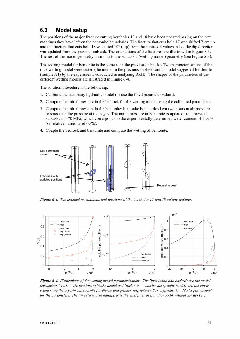
SKB P-17-05 61

Fractures with updated positions

Low permeable zones

Pegmatite vein

6.3 Model setupThe positions of the major fracture cutting boreholes 17 and 18 have been updated basing on the wet markings they have left on the bentonite boundaries. The fracture that cuts hole 17 was shifted 7 cm up and the fracture that cuts hole 18 was tilted 10° (dip) from the subtask d values. Also, the dip direction was updated from the previous subtask. The orientations of the fractures are illustrated in Figure 6-3. The rest of the model geometry is similar to the subtask d (wetting model) geometry (see Figure 5-3).

The wetting model for bentonite is the same as in the previous subtasks. Two parameterisations of the rock wetting model were tested (the model in the previous subtasks and a model suggested for diorite (sample A1) by the experiments conducted in analysing BRIE). The shapes of the parameters of the different wetting models are illustrated in Figure 6-4.

The solution procedure is the following:

1. Calibrate the stationary hydraulic model (or use the fixed parameter values).

2. Compute the initial pressure in the bedrock for the wetting model using the calibrated parameters.

3. Compute the initial pressure in the bentonite: bentonite boundaries kept two hours at air pressure to smoothen the pressure at the edges. The initial pressure in bentonite is updated from previous subtasks to −70 MPa, which corresponds to the experimentally determined water content of 11.6 % (or relative humidity of 60 %).

4. Couple the bedrock and bentonite and compute the wetting of bentonite.

Figure 6-3. The updated orientations and locations of the boreholes 17 and 18 cutting features.

Figure 6-4. Illustrations of the wetting model parametrisations. The lines (solid and dashed) are the model parameters (‘rock’ = the previous subtasks model and ‘rock new’ = diorite site specific model) and the marks o and x are the experimental results for diorite and granite, respectively. See ‘Appendix C – Model parameters’ for the parameters. The time derivative multiplier is the multiplier in Equation A-14 without the density.

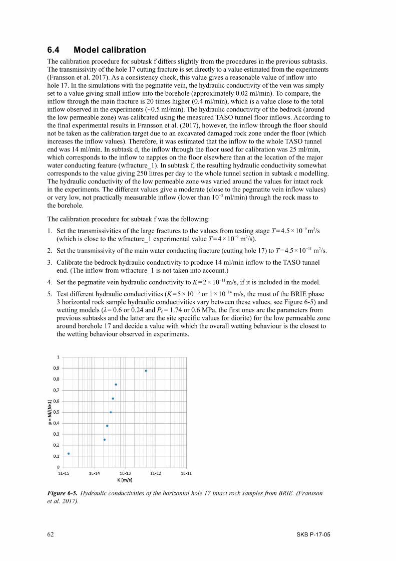
62 SKB P-17-05

6.4 Model calibrationThe calibration procedure for subtask f differs slightly from the procedures in the previous subtasks. The transmissivity of the hole 17 cutting fracture is set directly to a value estimated from the experiments (Fransson et al. 2017). As a consistency check, this value gives a reasonable value of inflow into hole 17. In the simulations with the pegmatite vein, the hydraulic conductivity of the vein was simply set to a value giving small inflow into the borehole (approximately 0.02 ml/min). To compare, the inflow through the main fracture is 20 times higher (0.4 ml/min), which is a value close to the total inflow observed in the experiments (~0.5 ml/min). The hydraulic conductivity of the bedrock (around the low permeable zone) was calibrated using the measured TASO tunnel floor inflows. According to the final experimental results in Fransson et al. (2017), however, the inflow through the floor should not be taken as the calibration target due to an excavated damaged rock zone under the floor (which increases the inflow values). Therefore, it was estimated that the inflow to the whole TASO tunnel end was 14 ml/min. In subtask d, the inflow through the floor used for calibration was 25 ml/min, which corresponds to the inflow to nappies on the floor elsewhere than at the location of the major water conducting feature (wfracture_1). In subtask f, the resulting hydraulic conductivity somewhat corresponds to the value giving 250 litres per day to the whole tunnel section in subtask c modelling. The hydraulic conductivity of the low permeable zone was varied around the values for intact rock in the experiments. The different values give a moderate (close to the pegmatite vein inflow values) or very low, not practically measurable inflow (lower than 10−3 ml/min) through the rock mass to the borehole.

The calibration procedure for subtask f was the following:

1. Set the transmissivities of the large fractures to the values from testing stage T = 4.5 × 10−9 m2/s (which is close to the wfracture_1 experimental value T = 4 × 10−9 m2/s).

2. Set the transmissivity of the main water conducting fracture (cutting hole 17) to T = 4.5 × 10−11 m2/s.

3. Calibrate the bedrock hydraulic conductivity to produce 14 ml/min inflow to the TASO tunnel end. (The inflow from wfracture_1 is not taken into account.)

4. Set the pegmatite vein hydraulic conductivity to K = 2 × 10−11 m/s, if it is included in the model.

5. Test different hydraulic conductivities (K = 5 × 10−13 or 1 × 10−14 m/s, the most of the BRIE phase 3 horizontal rock sample hydraulic conductivities vary between these values, see Figure 6-5) and wetting models (λ = 0.6 or 0.24 and P0 = 1.74 or 0.6 MPa, the first ones are the parameters from previous subtasks and the latter are the site specific values for diorite) for the low permeable zone around borehole 17 and decide a value with which the overall wetting behaviour is the closest to the wetting behaviour observed in experiments.

Figure 6-5. Hydraulic conductivities of the horizontal hole 17 intact rock samples from BRIE. (Fransson et al. 2017).

SKB P-17-05 63

6.5 Results6.5.1 Comparing the simulations with and without the pegmatite The first simulations in the subtask included pegmatite vein. These simulations, however, produce too fast wetting of bentonite, if compared to the experiments. The difference can be seen in the wrong shape of relative humidity graphs at the locations of the instrumented dry section (on the plane at −2.3 m from the top of the borehole) sensors (see Figure 6-6). Therefore, the pegmatite vein was removed from further simulations.

6.5.2 Comparison of simulations with different hydraulic conductivities for the low permeable zone

The plausible hydraulic conductivities for the low permeable zone basing on the experiments on BRIE phase 3 horizontal rock samples were tested. The values were K = 1 × 10−14 m/s and K = 5 × 10−13 m/s. The pegmatite vein was removed for the simulations and the wetting model for the rock from the previous subtasks was used. The higher conductivity value gives too fast wetting if compared to experiments (see Figure 6-7).

6.5.3 Comparison of different wetting models for the bedrockBefore the comparison of the different wetting models for the bedrock, the initial water content of bentonite in the model was slightly adjusted to make the simulated sensor 2 data to match the experimental data better than in Figure 6-7 and to get the simulated dry sensor RH values (sensors 1 and 3) below the measured ones. The short time of flooding experienced in the experiment (seen in the experimental data as initial peaking of the RH values) is not taken into account in the simulations and thus the simulated RH curves of dry sensors should not be on higher level than the experimental ones. The initial value for pressure in bentonite (the initial suction) was decreased from −70 MPa to −80 MPa. This change corresponds to decrease of water content from 11.3 % to 11.0 % (or the saturation from 0.41 to 0.39 or the relative humidity from 0.60 to 0.55).

Figure 6-6. A comparison of model results with and without pegmatite vein. The figure illustrates the relative humidity evolution at the sensor positions on the dry instrumented plane at −2.3 m. For sensor positions, see Figure 5-24. The solid lines represent model results with pegmatite vein (the upper graphs), the dashed lines without the vein (the lower graphs) and the crosses the experimental results. The difference in the shape between the modelling results should be noticed. The hydraulic conductivity of the low permeable zone is 1 × 10−14 m/s and the bentonite wetting model is the one used in previous subtasks.

64 SKB P-17-05

With the model geometry not including the pegmatite vein and with the new initial value for pressure in bentonite, the site specific wetting model was compared against the wetting model used in the previous subtasks. The results are illustrated with the graphs of the relative humidity at the sensor positions in Figure 6-8.

The relative humidity profiles in the direction of 216° clockwise from north at the dry instrumented level (−2.3 m from the borehole top) with the different model are drawn in Figure 6-9.

Figure 6-7. A comparison of model results with different hydraulic conductivities for the low permeable zone at the sensor positions. Sensor 1, 2 and 3 are on the wet instrumented plane at −2.6 m and sensor 4 is on the dry instrumented plane at −2.3 m from the hole 17 top. See Figure 5-24 for the sensor positions on the planes. The solid line presents results with K = 1 × 10−14 m/s, dashed lines with K = 5 × 10−13 m/s and crosses the experimental results. The wetting model for bedrock is the one in previous subtasks and there is no pegmatite vein in the simulations.

Figure 6-8. A comparison of the two wetting models for bedrock. The solid lines are relative humidity profiles at sensor position with the BRIE site specific rock wetting model (diorite), the dashed lines with the model from previous subtasks and crosses the experimental results. The model is without pegmatite vein, the hydraulic conductivity of the low permeable zone is K = 1 × 10−14 m/s.

SKB P-17-05 65

Figure 6-9. The relative humidity profiles in the direction of 216° clockwise from north at the dry instrumented level (−2.3 m from the borehole top). The lines are the model results with the previous subtask wetting model for bedrock and the dashed lines are results with the BRIE site specific wetting model. The circles and dots represent the experimental results for the rock and bentonite, respectively, at the time of dismantling of BRIE (at 14 months).

6.5.4 Results from the final simulationThe final comparison between the relative humidity sensor data and simulation data is presented in Figure 6-10. Comparisons of the hole 17 bentonite saturation patterns from the experiments and the simulations at different horizontal and vertical planes are illustrated in Figure 6-11, Figure 6-12 and Figure 6-13.

Figure 6-10. The relative humidity evolution at the sensor locations. Lines are the simulated results and the crosses the experimental ones.

66 SKB P-17-05

Figure 6-11. Saturation profiles of bentonite from the model and interpolated from dismantled bentonite block saturations. The heights from the bentonite bottom level are the following: 0.1 m, 0.3 m, 0.6 m, 0.9 m (instrumented level at −2.6 m from the bentonite top) and 1.2 m (instrumented level at −2.3 m from the bentonite top). The most saturated locations in the simulation results (left) somewhat correspond to the locations where the main fracture cuts the borehole 17.

Model Experiment

North

SKB P-17-05 67

Figure 6-12. Saturation of bentonite at different depths when the bentonite in hole 17 in BRIE was dis-mantled (the duration of wetting is 14 months and 8 days). The upper figures on each row are the model results and the lower ones interpolated from the samples taken of the BRIE dismantled bentonite blocks (Fransson et al. 2017). The approximate sensor positions on the planes at 0.9 m and 1.2 m are shown with white dots (position 1: WBR0001 and 4, position 2: WBR0002 and 5, position 3: WBR0003 and 6). Notice the differences of the wetting pattern in the especially in the bottom parts or the hole. Also, notice the difference on the most saturated part on the 0.9 m height from the borehole bottom (corresponding to the wet instrumented plane at the depth of −2.6 m from the borehole bottom). North is up.

0 m (from bottom) 0.25 m 0.45 m 0.55 m

0.65 m 0.85 m

3

1

2

0.9 m (−2.6 m plane) 1.2 m (−2.3 m plane)

68 SKB P-17-05

Figure 6-13. Vertical saturation profiles of the bentonite in different directions (from north) below −2.3 m level from the top of the bentonite after dismantling BRIE (model at 14 months). The model results are on the top and the experimental results are on the bottom row. The left halves of the experimental results are at the plane from which the samples have been taken. The right halves have been intrapolated.

0° 72° 144° 216° 288°

SKB P-17-05 69

Figure 6-14. The relative humidity profiles across the bentonite rock interface in the direction of 0° clockwise from north at 20 cm above the dry instrumented level (−2.1 m from the borehole top). The lines are model results whereas the circles and dots represent the experimental results for the rock and bentonite after dismantling BRIE (after 14 months).

Figure 6-15. The relative humidity profiles across the bentonite rock interface in the direction of 216° clockwise from north at the dry instrumented level (−2.3 m from the borehole top). The lines are the model results whereas the circles and dots represent the experimental results for the rock and bentonite, respectively, at the time of dismantling BRIE (14 months).

Relative humidity profiles through the bentonite rock interface at different sections (−2.1 m, −2.3 m and −2.7 m below the bentonite top level) and directions (0° or 216° clockwise from north) are illustrated in graphs in Figure 6-14, Figure 6-15 and Figure 6-16. The experimental results for bentonite are of samples from 10 cm below to 10 cm above the planes into the different directions. The experimental results for the rock are approximately at the corresponding levels and directions at the rock wall.

The simulated total saturation evolution of bentonite is shown in Figure 6-17.

70 SKB P-17-05

Figure 6-16. The relative humidity profiles across the bentonite rock interface in the direction of 216° clockwise from north at 10 cm below the wet instrumented level (−2.7 m from the borehole top). The lines are the model results whereas the circles and dots represent the experimental results for the rock and bentonite, respectively, at the time of dismantling BRIE (14 months).

Figure 6-17. The evolution of the total saturation of bentonite in borehole 17 (integrated over the bentonite volume). The times to 95 % average saturation are 40 years without pegmatite vein and 6 years with pegmatite vein.

SKB P-17-05 71

6.6 Discussion6.6.1 Wetting characteristics of bentonite in the final simulation With the final model, the simulation results show surprisingly good agreement with the experimental results, but it is also evident that some of the feature in the experiments cannot be captured with the model here.

The comparison of the relative humidities at the sensor locations (Figure 6-10) show very good agreement for sensors at the dry instrumented plane (at −2.3 m from the tunnel floor) and sensor WBR0002 (sensor 2) on the wet instrumented plane. After the initial peaks of relative humidity in the experiment (by the short period of flooding), the experimental relative humidities seem to decrease to similar levels as in the simulation, after which the graphs can be said to coincide within the accuracy of the simulation. The sensors 1 and 3 seem to follow the trend of the sensor data, but the level is incorrect. Sensor 1 is located close to the central shaft, through which the flooding in the experiments occurred. This might partly explain the higher relative humidity in the experimental results than in the simulation.

Sensor 3 is located near the fracture at the −2.6 m level. Unlike in the case of the sensor further away from the water sources (2, 4−6), it seems that there is no time for the sensor 3 to recover from the flooding before it wets again (compare to RH decrease for sensors 2, 4−6). This could plausibly cause the high relative humidity level in the experiment at that location. The uncertainty in the main fracture location (due to the uneven shape of the fracture) in the model could also possibly affect the relative humidity increase rate, although Figure 6-12 (plane at 0.9 m or −2.6 m from the tunnel floor) suggests that the model fracture position is closer to the sensor than the real one in the experiment. The difference in the relative humidities at sensor 3 position may also mean that the wetting model for the bentonite is incorrect. If taken a look at the relative humidity graphs at on horizontal lines in different directions (Figure 6-14, Figure 6-15 and Figure 6-16), it is clear that the wetting model for bentonite produces too sharp relative humidity profiles near the bentonite edge, if compared to experiments. Therefore, the inaccurate wetting model may cause the relative humidity at sensor 3 location to take longer time to reach the similar level in the simulation as in the experiments.

The saturation patterns in Figure 6-11, Figure 6-12 and Figure 6-13 clearly illustrate that a number of water conducting features are lacking from the bottom part of the borehole 17 in the model and that the main fracture does not conduct water evenly (or is not of planar shape) in the experiment as assumed in the model. At some locations, however, the main fracture produces similar fast wetting as in the experiment. The small features have a local effect on the wetting pattern, but (with the final parametrisation of the model) the total wetting time of the whole bentonite cylinder seems to be dictated by the maximum length of a dry section of the bentonite surrounding bedrock. Therefore, the main fracture could be thought to dominate the wetting behaviour in the bottom section, whereas the total wetting time is a result of the length of the upper dry section.

6.6.2 The effect of the pegmatite veinAs logical, the inclusion of the pegmatite vein in the model produces faster wetting of bentonite than without the vein. Especially, the wetting rate in the dry section of hole 17 is too fast if compared to the experiment (compare the dry section relative humidity graphs in Figure 6-6). Therefore, the vein was removed from the model in the final stage. In retrospect, it would have been a good idea to include the vein around the lower part of bentonite, where the main fracture does not seem to produce fast enough wetting if compared to the experiments.

The wetting rates from the simulation with pegmatite vein at the dry instrumented section of hole 17 seem to somewhat match the rates in the experiment at the dry instrumented section of hole 18 (see Figure 6-18). Hole 18 walls being more fractured than hole 17 walls (see Figure 6-1), the simulation with the pegmatite vein could be interpreted to represent a case, in which there is some fracturing of bedrock around the bentonite in addition to main water conducting fractures.

72 SKB P-17-05

6.6.3 The effect of the hydraulic conductivity of the low permeable zoneAs noticed already in the previous subtasks, the hydraulic conductivity of the low permeable zone has a great impact on the wetting time of bentonite. If the value is high (clearly over K = 1 × 10−14 m/s, see simulated results with K = 5 × 10−13 m/s in Figure 6-7) bentonite wets basically in 10 months (see subtask c and d results) according to the simulations. If the value is lower than K = 1 × 10−14 m/s, the bentonite wets through the features explicitly included in the model as discrete features. The problem is that both the values are plausible according to the tests on dismantled de-stressed rock samples (see Figure 6-5). It seems, however, that for most samples the value is closer to K = 1 × 10−14 m/s (below K = 5 × 10−14 m/s) than to K = 5 × 10−13 m/s. The stress of bedrock also probably decreases the value in-situ.

Basing on comparison of simulated relative humidity graphs at the sensor locations to the experimental ones, it seems that the permeability value for the rock mass in the low permeable zone is on the level of intact rock mass in the experiments (K = 1 × 10−14 m/s) and that all the water bearing features should be added to the model as geometrical extra features excplicitly. As the wetting rate is highly sensitive to hydraulic conductivity value, the bentonite wets too quickly if the small features are incorporated into the low permeability value. In this view, the concept proposed in subtask d (i.e. the rock mass in the low permeable zone accounts for the small fractures) had to be updated to a one with separated intact rock mass and water conducting features.

6.6.4 The wetting modelsIf the different wetting models for bedrock (the previous subtask model and the site specific diorite model) are compared, there seems to be only small differences. The wetting rate seems to the slower for the diorite model (see Figure 6-8) than for the previous subtasks model. The difference is, however, small if compared to effects by other parameter choices (e.g. the initial suction values in the bentonite). The difference can be traced back to the wetting model parametrisations illustrated in Figure 6-4. The relative permeability for both the models is many orders of magnitude lower than the value for bentonite wetting model at all pressures and the time derivative multipliers are somewhat the same if compared to the curve for bentonite. If the total hydraulic conductivity (relative permeability times the hydraulic conductivity) is below the limit K = 1 × 10−14 m/s, the value has no particular effect on the wetting behaviour as the bentonite wets through the discrete features. Therefore, the expected outcome of the parametrisations is approximately the same wetting behaviour with both the bedrock wetting models.

Figure 6-18. Comparison of the simulated relative humidity profiles with pegmatite vein at the dry section of hole 17 (sensors 4–5) to the experimental relative humidity profiles at the dry section of hole 18 (sensors 10–12).

SKB P-17-05 73

Comparison of the relative humidity graphs on the horizontal lines in different directions from the simulation to the experimental ones (see Figure 6-9, Figure 6-14, Figure 6-15 and Figure 6-16) reveals that all the wetting models (both the bedrock models and the model for bentonite) perform quite badly. The simulations result in extremely steep gradient for relative humidity (also for pressure and saturation) near the bedrock-bentonite interface, but the graphs of experimental results show much gentler slope. The difference indicates that the wetting models are simply wrongly parameterized. To get to bottom of this problem, one has to start by thinking of what the wetting model parametrized are actually based on. The basic, underlying assumption of the original work on the wetting models (by e.g. van Genuchten and Brooks and Corey) is that the water moves in a porous medium by capillary action (that is, the suction is capillary suction and no adsorption is taken into account). Especially, the functional forms for the relative permeability rely on this assumption. Now, these functions are used for bentonite, even though the suction is complete dominated by physico-chemical adsorption of water on montmorillonite mineral (interlayer and stack outer) surfaces (see order of magnitude for the values of negative pressure in the model). In other words, the shapes of the wetting parameters have nothing to do with the wetting phenomenology of bentonite. To make this worse, the wetting models produce very nonlinear functions to be solved when they are used out of their originally intended range like the rock wetting model at completely dry range (pressure is less than −5 MPa in Figure 6-4) in the simulations here. As a results of all this, the wetting model for bentonite should be considered as a fit of unnecessarily complicated and nonlinear functions to experiments producing behaviour (somewhat steeply advancing wetting fronts) that is not observed in experiments. Besides the relative humidity graphs cutting the rock-bentonite interface, one can see the effect of the parameter shapes in only slowly spread saturation in the model wetting pattern figures if compared to the exper-imental ones. It should, however, be noted that the experimental patterns are affected by the real water source shapes (that are wider than the discrete fracture) and interpolation procedure. Having written all this, the simulated results agree in many aspects surprisingly well with the experiments, because the wetting through the intact rock is dominated by wetting through the distinct water con-ducting features. If the water source is at full saturation (as the distinct fractures in the model are), the wetting model for bentonite produces temporally somewhat correct behaviour with respect the total saturation of bentonite as suggested already by the simulation of the water uptake test in Appendix F (see especially Figure F-1).

If the wetting phenomenology is put aside for now and just the values of the parameters are con-centrated on, the basic problem with the wetting models are the very high suction values (i.e. very low pressures) needed for bentonite. With these values (at the rock-bentonite interface), the wetting models for rock produce extremely low relative permeability values if compared to bentonite (see Figure 6-4). Thus, also the total hydraulic conductivities (relative permeability times the hydraulic conductivity) vary at the interface by several orders of magnitude. This large difference combined with the extremely low total hydraulic conductivity for bedrock results in equally extreme gradient in the pressure that is solved from the equations (see Figure 6-19). As the total hydraulic conductivity in the rock is lower than in bentonite, the pressure gradient is located in the rock side of the interface. The dismantled BRIE results (see Figure 6-9, Figure 6-14, Figure 6-15 and Figure 6-16), however, show that the relative humidity profiles at both sides of the interface curve towards the interface. This indicates that the total hydraulic conductivities of both the bentonite and the bedrock should actually be close to each other or at least not to differ by orders of magnitudes. When pressure level at the interface increases in time and the relative permeability in the bedrock gets closer to one, the relative humidity profiles begins to curve to a shape closer to the experimental profile than in the earlier times when the profile is basically a step function-like.

6.6.5 Water conducting features at the rock-bentonite interfaceThe exact locations and shapes of the water sources wetting the bentonite could be determined only after dismantling BRIE and taking a look at the bentonite parcel surface. The major water conducting features were observed before the bentonite was installed into the boreholes, but many of the smaller water conducting features were missed or, at least, they could not be distinguished from the features seen but not conducting water. Also, if a fracture cutting a borehole conducts water, it does not necessarily conduct it evenly (in a sense of smooth even fractures in the model) but the flow paths can result in pointwise wetting sources. To capture the exact wetting behaviour of bentonite by modelling, the locations and shapes of the water conducting features should be known. Therefore, in addition to experimental techniques to find the fractures that cut the boreholes (such as BIPS),

74 SKB P-17-05

techniques to find which of them (or of other features) conduct water should also tried to be developed to a level that they could be easily used in the final repositories. One option to circumvent the direct techniques could be to try to correlate the number of fractures to the conductivity or to try to correlate stress of bedrock to the conductivity (for an initial attempt to do this see subtask d).

6.6.6 Model concept: Geometry The concept of dividing the model geometrically to somewhat detailed parts (near the bedrock-bentonite) and to less detailed parts (the EPM rock further away from the interface) seems to be a reasonable simplification. As a result, the model size (the number of degrees of freedom) can be kept relatively small meaning that it can be solved with a desktop computer instead of a computer cluster.

Maybe the most significant drawback of not having a discrete fracture network outside the low per-meable zone is related to the connectivity of the water conducting features in the zone. If a fracture (or other feature) cuts the low permeable zone and is thus connected to the EPM rock, the fracture is automatically well connected to everywhere in the rock. This causes problems in including poorly connected water sources to bentonite that can leave a wet mark on the bentonite surface but that can be drained completely after a short period due to suction by bentonite and slow rewetting through the poor connected surrounding rock. Such features might be seen on the bentonite outer surface in the experiments but they might not contribute significantly to the total wetting due to the limited amount of water that can be drawn from them.

In principle, it is easy to add many features to the low permeable zone, but with the current wetting model for the bentonite and the bedrock this easily leads to a non-convergent model, if a meaningful sized mesh is used in the computation. The wetting models lead to an unrealistically steep pressure gradient (if compared to BRIE results) at the interface which cannot be captured with the numerical methods used to solve the model here (the spatial discretization with the (continuous Lagrange-Galerkin) finite element method, time-wise discretization with the adaptive various step-size, various order backwards differentiation formula (practically implicit Euler in the simulations here), damped Newton’s method as the nonlinear solver (with initial damping factor around 0.01 and 3–5 times maximum

Figure 6-19. A close-up picture of the pressure drop in the rock near the interface in a dry section at 1 month (blue solid line) and 1.5 years (red dashed line). The pressure drops from above zero values to −50 MPa within approximately 0.2 mm (which is the element size at the interface) due to the combination of low total hydraulic conductivity and the relative permeability difference between bentonite and bedrock.

rock

bentonite

SKB P-17-05 75

damping factor increase per iteration) and a direct linear system solver (MUMPS)). The steep gradient is a direct consequence of the total permeabilities (the relative permeability times the Darcy permeability) of bentonite and rock at the interface differing by orders of magnitudes at high suctions (see Figure 6-4 for the relative permeability differences). As a consequence of this inbuilt feature, the gradient at the interface produced by the model remains steep unless the model parameters are drastically changed. Such change would, however, likely make the model perform poorly when simulating wetting of bentonite from fully saturated water sources (e.g. the water uptake test in Appendix F). If the current wetting model for bentonite would be replaced with a phenomenology and conceptually more reason-able one, the ability add the small features to the model with acceptable computational cost might increase considerably.

Although the main wetting sources of bentonite can be captured with the geometrically flat discrete (two dimensional) surfaces in the model, it is evident that this concept fails to produce some of the wetting features observed in BRIE. For example, the water source from the main fracture cutting hole 17 does not follow the fracture-bentonite interface evenly, but there are clear wet and relatively dry points on it. Similarly, there seems to be a number of features on the rock-bentonite interface that give a somewhat randomly shaped and located inflow of water to bentonite, if compared to the known (from the analysis of the rock) fractures and other features.

6.6.7 Rock mechanical effectsThe surface of the dismantled bentonite parcel shows wet markings in vertical direction of boreholes walls for both holes 17 and 18 (see Figure 6-1). The markings do not correlate to fractures or other water conducting features seen prior to the installation of bentonite in neither the probing nor the enlarged boreholes. A possible explanation for the markings could be new fractures generated by the change in bedrock stress when the boreholes have been drilled. If taken a look at the stress levels at the borehole surfaces computed in subtask d (and recomputed in subtask f) in Figure 6-20, one can see that the compressive stress (pressure) has negative values approximately on the borehole 17 side walls directed to the side walls of the tunnel end (dark blue colour in the left figure). This direction corresponds to the location of the vertical fractures seen on the bentonite surface. Vibrations or ground-water pressure changes together with these tensile stress values may cause the failure criterion for stress to be exceeded and new fractures to be generated. The failure behaviour of rock, however, is not this simple, since also the von Mises (deviator) stress plays a part in the failure criterion which often follows Mohr-Coulomb (or Drucker-Prager) failure surfaces for rocks. As the von Mises stress is the lowest at the points where the tensile stresses occur, it is not clear in which direction the rock preferably fails, although the tensile stress direction could be considered the likely direction.

Figure 6-20. Pressure (left) and von Mises shear stress (right) on the borehole 17 surface. Borehole 18 on the left is in the figures to show the direction related to the TASO tunnel end. The pressure is negative on left hand side figure indicating tensile stress on part of the borehole surface. On the other hand, von Mises stress causing the yielding (or failure) in shear direction is the lowest at the points where the pressure is the lowest.

Pressure (Pa) von Mises stress (Pa)

76 SKB P-17-05

As the stress values tend to increase when the borehole diameter grows and the final disposal bore-holes are wider than the BRIE holes, the possible correlation between the new fracture generation and the local stress state near the boreholes should be further investigated. Also the possible closure of these fractures when the bentonite swelling stress evolves could be worth studying.

Application of the rock mechanical model used in subtask d for the final modelling step would have been interesting, but such modelling is out of the scope of this study. If the mechanically coupled model is used in wetting simulations with the current parametrization of the low permeability zone (lower hydraulic conductivity than in subtask d), similar convergence problems as when adding many geometrical features in the low permeable zone are met. This is again result of using the highly nonlinear wetting models. In this case, however, the problems are in some view even more severe, since the hydraulic conductivity (or permeability) tensor follows the principal stress coordinates that are not as regular as standard Euclidean space coordinates.

6.6.8 The effects of deformation and stress of bentonite during wettingAlthough fully coupled models for bentonite are out of scope of this study and bentonite is considered as a mechanically inert material in the modelling here, in reality the mechanical, wetting and chemical behaviour of it are strongly coupled. In X-ray tomography analysis of bentonite wetting in Harjupatana et al. (2015), it is for example noticed that the water contents by the tomography and the dismantled samples do not correlate well if the deformation of bentonite is not taken into account. Therefore, ignoring the mechanical effects in the modelling of BRIE introduces some error in the results, since the dry density of bentonite is observed to change (that is, bentonite deforms) during the wetting (see Figure 6-21).

Another source of error in the simulation is the water retention curve for bentonite, which bases on the retention data from bentonite powder (destressed bentonite). If compared to the in situ (stressed bentonite) data from dismantled BRIE bentonite parcel, the retention curve used in the simulations shows too high water content (see Figure 6-22).

Besides the effects of stress and deformation on bentonite itself, the increasing swelling stress of bentonite also affects the stress state of the surrounding bedrock. As the bedrock stress, in turn, may affect the water flow in bedrock, the swelling stress evolution during wetting increases the uncertainties also related to the water flow.

Figure 6-21. The dry density of bentonite in hole 17 after dismantling. Figure by Mattias Åkesson.

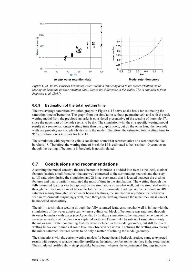
SKB P-17-05 77

6.6.9 Estimation of the total wetting timeThe two average saturation evolution graphs in Figure 6-17 serve as the basis for estimating the saturation time of bentonite. The graph from the simulation without pegmatite vein and with the rock wetting model from the previous subtasks is considered presentative of the wetting of borehole 17, since the upper part of the hole seems to be dry. The simulation with the site specific wetting model results in a somewhat longer wetting time than the graph shows, but on the other hand the borehole walls are probably not completely dry as in the model. Therefore, the estimated total wetting time to 95 % of saturation is 40 years for hole 17.

The simulation with pegmatite vein is considered somewhat representative of a wet borehole like borehole 18. Therefore, the wetting time of borehole 18 is estimated to be less than 10 years, even though the wetting of bentonite in borehole is not simulated.

6.7 Conclusions and recommendationsAccording the model concept, the rock-bentonite interface is divided into two: 1) the local, distinct features (mainly small fractures) that are well connected to the surrounding bedrock and that stay at full saturation during the simulation and 2) intact rock mass that is located between the distinct features and that is partially saturated the most of time in the simulations. The wetting through the fully saturated features can be captured by the simulations somewhat well, but the simulated wetting through the intact rock cannot be said to follow the experimental findings. As the bentonite in BRIE saturates mainly through distinct water bearing features, the simulations reproduce the behaviour seen in experiments surprisingly well, even though the wetting through the intact rock mass cannot be modelled successfully.

The ability to simulate wetting through the fully saturated features somewhat well is in line with the simulations of the water uptake test, where a cylindrical block of bentonite was saturated through its outer boundary with water (see Appendix F). In those simulations, the temporal behaviour of the average saturation of the block was captured well (see Figure F-1). In subtask f simulations, only the major small water conducting features were included in the model geometry, but still the overall wetting behaviour reminds at some level the observed behaviour. Capturing the wetting also through the minor saturated features seems to be only a matter of refining the model geometry.

The simulations with the current wetting models for bentonite and bedrock produce some unexpected results with respect to relative humidity profiles at the intact rock-bentonite interface in the experiments. The simulated profiles show steep step-like behaviour, whereas the experimental findings indicate

Figure 6-22. In-situ (stressed bentonite) water retention data compared to the model retention curve (basing on bentonite powder retention data). Notice the differences in the scales. The in situ data is from Fransson et al. (2017).

Model retention curveIn situ water retention data

78 SKB P-17-05

that the step should be gentler and smoother. The simulated steep profiles seem to result from the many orders of magnitudes difference in the total permeabilities of bentonite and rock at the interface. The permeabilities, in turn, result from the used van Genuchten type of wetting models for bentonite and rock. Because the wetting model parameters are defined by well conducted experiments, this suggests that the root cause for the deviating simulated and experimental profiles lies in the concepts behind these wetting models. Therefore, it is recommended that the phenomenological and conceptual basis for the wetting models is re-evaluated, especially for bentonite. The nonlinearities arising from the models also prevent further refinement of the model geometry and coupling the wetting to e.g. rock mechanics.

With the current model, the wetting time for bentonite in hole 17 is estimated to be 40 years. The result yields from the long dry section in the borehole and wetting model parametrisation such that the bentonite wets through fractures and not through the rock mass surrounding the borehole. Basing on the hole 17 simulations parametrised for a wet borehole, the wetting of bentonite in borehole 18 is estimated to take less than 10 years.

SKB P-17-05 79

7 Concluding summary

The five subtasks led to a development of a model concept that combines discrete fractures and features at the bentonite rock interface and equivalent porous medium (EPM) elsewhere. The key objects of the model are the bentonite filled borehole, the small discrete fractures and pegmatite vein cutting the boreholes, the EPM low permeable zone around the boreholes, the large deterministic fractures and, of course, the rest of the fractured bedrock where EPM concept is used.

The objects define a model that includes geometrically detailed features near the bentonite-bedrock interface and that can be calibrated with a relatively small amount of experimental data. The bedrock hydraulic model can also be coupled to the bedrock stress. Nonetheless, the computational work required to solve the model is sufficiently low.

The largest uncertainty of the model is related to the hydraulic conductivity of the rock mass near the boreholes, that is, the low permeable zone. Depending on the properties of this zone, the models produce wetting time estimates ranging from approximately ten months to 50 years for the compacted bentonite cylinder of 30 diameter surrounded by bedrock in BRIE. Only if the permeability of this zone is very low, the positions of the fractures and other well water conducting features decide the wetting behaviour of the bentonite. Otherwise, bentonite wets through the rock mass in approximately 10 months.

Utilizing the final experimental results from BRIE, the simulated wetting time for a bentonite in a borehole with a long dry section specifies to 40 years (borehole 17) and for a borehole with water sources through the height (somewhat similar to borehole 18) of it to less than 10 years.

Comparing the simulated results to the full experimental data from BRIE enhances the understanding of the bentonite rock interface. The comparison reveals that the bentonite wets mainly through specific water sources in the bedrock such as small fractures and not that much through the intact rock mass. It is found out that the effect of the small fractures cannot be averaged to form an equivalent porous media around the borehole in a model but they have to be included explicitly in the model. Otherwise, the model produces too fast wetting of bentonite. If only the major water conducting features are included in the model, the wetting time of bentonite can be estimated roughly. Then, however, the local wetting patterns of bentonite resulting also from the minor water conducting features cannot be reproduced by the simulations.

The simulations show that the geometry of the main water sources dictates the wetting time of bentonite. The longest dry section of a borehole rock wall can be said to determine the wetting time. The specific values of parameters for water conducting features, such as the transmissivities of the fractures, are not important as long as the feature provides water to bentonite. The effect of the con-nectivity of the water conducting features was not studied here, as all the features providing water to bentonite are well connected to the water sources further away in the bedrock.

When assessing the performance of the model concept, it is useful to divide the water sources for bentonite into two: 1) the local, distinct features (mainly small fractures) that are well connected to the surrounding bedrock and that stay at full saturation during the simulation and 2) intact rock mass that is located between the distinct features and that is partially saturated the most of time in the simulations. The wetting through the fully saturated features can be captured by the simulations somewhat well. Because the bentonite in BRIE saturates mainly through such features, the wetting simulations reproduce the overall behaviour seen in experiments surprisingly well. On the other hand, a comparison of the simulated and experimental relative humidity profiles across the intact rock-bentonite interface shows that the used wetting models cannot capture the water transport from intact rock to bentonite (or vice versa) correctly. The deviation seems to result from the many orders of magnitudes difference in the total permeabilities of bentonite and rock at the interface, which, in turn, results from the used van Genuchten type of wetting models for bentonite and rock. Because the wetting models have been experimentally calibrated, the root cause for the deviating simulated and experimental profiles seems to lie in the concepts behind these wetting models. Therefore, it is recommended that the phenomenological and conceptual basis for the bentonite and rock wetting models should be re-evaluated.

80 SKB P-17-05

The mechanical coupling of the bedrock hydraulic model proves to be useful mostly when examining the inflow to open boreholes. The coupling provides some insight into effect of stress on the water flow patterns. On the other hand, the small deviations in the hydraulic parameters for bedrock result-ing from the coupling seem to have very limited effect on the wetting of bentonite, at least when the wetting of bentonite is dominated by flow through rock matrix. This observation is in line with the seen small effect of changing the hydraulic parameters of the fractures in the non-coupled models. As the geometry of the water conducting features is important, a mechanically coupled model could be, however, useful when studying the opening of new fractures because of the changes in bedrock stress by e.g. a drilled hole and the closure of old fractures because of the swelling pressure of bentonite.

SKB P-17-05 81

8 References

SKB’s (Svensk Kärnbränslehantering AB) publications can be found at www.skb.com/publications.

Bai M, Meng F, Elsworth D, Zaman M, Roegiers J-C, 1997. Numerical modeling of stress-dependent permeability. International Journal of Rock Mechanics and Mining Sciences 34, 2-e1–2.e14.

Vidstrand P, Stigsson M, Åkesson M, Fransson Å, 2017. Task Forces EBS and GWFTS. Modelling the interaction between engineered and natural barriers. A compilation of Task 8 descriptions. SKB P-16-05, Svensk Kärnbränslehantering AB.

Carrier W D, 2003. Goodbye, Hazen; hello, Kozeny-Carman. Journal of Geotechnical and Geoenvironmental Engineering 129, 1054–1056.

Dueck A, 2004. Hydro-mechanical properties of a water unsaturated sodium bentonite: laboratory study and theoretical interpretation. PhD thesis. Lund University, Sweden.

Edlefsen N E, Anderson A B C, 1943. Thermodynamics of soil moisture. Hilgardia 15, 31–298.

Fransson Å, Åkesson M, Andersson L, 2017. Bentonite Rock Interaction Experiment. Characterization of rock and installation, hydration and dismantling of bentonite parcels. SKB R-14-11, Svensk Kärnbränslehantering AB.

Fredlund D G, Rahardjo H, 1993. Soil mechanics for unsaturated soils. New York: Wiley.

Gangi A F, 1978. Variation of whole and fractured porous rock permeability with confining pressure. International Journal of Rock Mechanics and Mining Sciences & Geomechanics abstracts 15, 249–257.

Harjupatana T, Alaraudanjoki J, Kataja M, 2015. X-ray tomographic method for measuring three-dimensional deformation and water content distribution in swelling clays,. Applied Clay Science 114, 386–394.

Kahr G, Kraehenbuehl F, Stoeckli H F, Müller-Vonmoos M, 1990. Study of the water-bentonite system by vapour adsorption, immersion calorimetry and X-ray techniques: II. Heats of immersion, swelling pressures and thermodynamic properties, Clay Minerals 25, 499–506.

Kajanto K, 2013. The effect of stress state on groundwater flow in bedrock: simulations of in situ experiments. Espoo: VTT (VTT Technology 127)

Kim J M, Parizek R R, 1999. A mathematical model for the hydraulic properties of deforming porous media. Ground Water 37, 546–554.

Min K-B, Rutqvist J, Tsang C-F, Jing L, 2004. Stress-dependent permeability of fractured rock masses: a numerical study. International Journal of Rock Mechanics and Mining Sciences 41, 1191–1210.

Pruess K, Oldenburg C, Moridis G, 2012. TOUGH2 User’s guide, version 2.1. Report LBNL-43134, Lawrence Berkeley National Laboratory, Berkeley, CA.

Swan G, 1983. Determination of stiffness and other joint properties from roughness measurements. Rock Mechanics and Rock Engineering 16, 19–38.

Talbot C J, Sirat M, 2001. Stress control of hydraulic conductivity in fracture saturated swedish bedrock. Engineering Geology 61, 145–153.

SKB P-17-05 83

Appendix A

The wetting and flow model equations Four types of major processes are considered in our model: the flow of water in fully saturated bed-rock and fractures, possible drying and re-saturation of the bedrock and fractures near the bentonite, the flow of water in fully saturated bentonite and the wetting of bentonite.

Flow of water in fully saturated conditionsThe flow of water in saturated conditions is governed by mass balance equation, Darcy’s law and the state equations relating pressure to the density of water and to the solid volume fraction. In this formulation, pressure difference is considered as driving force of the water flow and the viscous effects can be averaged to the Darcy velocity due to the random structure of the porous medium. In the fractures, the parabolic velocity profile is also replaced by the average water velocity.

The mass balance equation simply reads

( )( ) 0t

φρ ρ∂ + ∇ ⋅ =∂

u (A-1)

where ϕ is the porosity, ρ the density of water, p the pressure of water and u the Darcy velocity, which, in turn, is defined by Darcy’s law:

µ ( )pκρ= − ∇ −u g . (A-2)

The time derivative term of the mass balance equation can be expanded with the chain rule as follows

( ) ( ) p pt p t p p t

φρ φρ φ ρρ φ ∂ ∂ ∂ ∂ ∂ ∂= = + ∂ ∂ ∂ ∂ ∂ ∂ (A-3)

where

s1 (1 )(1 ) (1 )

1p pφ φφ φ χ

φ ∂ ∂ −= − ⋅ − = − ∂ − ∂

(A-4)

and

f1

p pρ ρφ ρφ ρφχ

ρ∂ ∂= =∂ ∂

(A-5)

resulting in

( )s f s( ) (1 ) p pS

t t tφρ ρ φ χ φχ ρ∂ ∂ ∂= − + =∂ ∂ ∂

(A-6)

where χs and χf are the compressibilities of solid and fluid respectively and Ss the specific storage coefficient.

The above equations put together give a single equation from which the pressure can be solved:

( )s 0pS pt

κρ

µ ∂ + ∇ ⋅ − ∇ − = ∂

g . (A-7)

The flow of water in partially saturated conditionsThe above potential flow equation for fully saturated porous media can extended to unsaturated con-ditions. In the extension, pressure below gas pressure is considered as a measure of suction potential. Also, the concepts of saturation, S, and relative permeability, kr, are introduced.

84 SKB P-17-05

The continuity equation takes the form

( )( ) 0Stφρ

ρ∂ + ∇ ⋅ =

∂u (A-8)

and the infiltration velocity becomes

( )rk pκρµ= − ∇ −u g . (A-9)

A relation between saturation and pressure is needed in order to solve one of them from the resulting equation. The relation is called retention curve, for which van Genuchten formulation is used:

11

g l

0

( ) 1p p

S pp

λ

λ

−

− − = +

. (A-10)

Here λ and p0 are fitting parameters. The cubic law for the relative permeability of bentonite is

kr = S3 (A-11)

and the van Genuchten relative permability that is used for bedrock reads2

1

r 1 1lk S Sλ

λ = − −

, (A-12)

where λ is a fitting parameter. (In subtask 8c, TOUGH2 uses this relation also for bentonite.)

Since the nature of the pressure in the unsaturated conditions is not “real” pressure but a measure of capillary and chemical phenomena that induce suction, the pressure in unsaturated conditions is unlikely to compress the water or the solid of the porous medium. Therefore, the time derivative can be expanded as

1 1

0

( ) ( ) 1 ( ) 1 ( )1

S S p p pS p S pt p t p t

λ

λ λφρ λρφ ρφλ

∂ ∂ ∂ ∂= = − ∂ ∂ ∂ − ∂ . (A-13)

If the saturated zone multiplier in Equation A-4 is extended to the unsaturated zone to make the whole time derivative multiplier continuous over the saturated-unsaturated interface, the term becomes

1 1

s0

( ) 1 ( ) 1 ( )1

S pS p S p St p t

λ

λ λφρ λρφ ρλ

∂ ∂ = − + ∂ − ∂ , (A-14)

which is not strictly physical but does not introduce much of error it the specific storage coefficient is not too large.

The wetting model is based on an idea that the flow of water in partially saturated bentonite is driven by water potential gradient. A one-to-one relation between the water content (or saturation) and the potential can be found by equilibrating bentonite with water vapour at certain partial pressures (or relative humidities) and measuring the water content. The equilibrium vapour potential converted to units of joule per volume is taken as the suction value. Here, Kelvin (or Kelvin’s) equation is used:

porouswater

water free

lnpRTs

M pρ

=

, (A-15)

where s is the suction, ρwater the density of water, R the universal gas constant, T the temperature, Mwater the molecular weight of water, ρporous the measured partial vapor pressure in the porous medium and ρfree the saturation vapor pressure of free water surface. Then, the traditional soil wetting equations with the obtained retention curves are used. The citations often pass through the chain (Dueck 2004, Kahr et al. 1990, Fredlund and Rahardjo 1993, Edlefsen and Anderson 1943).

SKB P-17-05 85

The flow of water in the fracturesThe fully and partially saturated flow equations are solved with finite element method. This allows us to describe the flow of water in fractures in two dimensions instead of to the three dimensional description of the flow in the rock matrix and in bentonite. If a wetting type of equation is written in weak form,

3d 3dtest test test( ) ( ) 0pa p p b p p p dV p dS

tΩ ∂Ω

∂ ∇ +∂∫ j n· =∫+ ·∇ , (A-16)

one dimension of the integrations can be replaced by the aperture of a fracture, δ, as follows

2d 2dtest test test( ) 0p

tδδ

Ω ∂Ω

∂∂

j n· =∫ ∫a p b Sd l∇+ ∇ +||||p ( )p p · p p d . (A-17)

In this formulation, the two dimensional integrations is taken along the fracture plane and the gradients in three dimensions, ∇, have been replaced by gradients in the fracture tangent direction ∇||. In this formulation, the Neumann, i.e. the flux, boundary conditions have to be pointed on the edges of the fractures instead of boundaries. Also, the Diriclet boundaries, i.e. the constraints, have to be placed on the edges instead of the boundaries.

The apertures of the large fractures have been obtained from Task description, whereas the apertures of the small fractures are assumed to be related to their transmissivities. If water is thought to flow between parallel plates, a relation

312T

gµδ

ρ= (A-18)

can be derived for the aperture.

Combining the flow conditions into one modelSaturated and unsaturated water flow equations can be combined simply by stating that pressure p is the water pressure when p ≥ pgas and a measure of suction when p < pgas. Moreover, the coefficients in the equations have to match when on the fully and partially saturated parameter range interface p = pgas. If the storage term Ss is sufficiently small, the parameter matching can be done by extending the use of storage term into the unsaturated conditions (Equation A-4), although it has no clear physical meaning in these conditions. The relative permeability is automatically correct in the fully saturated conditions: kr = 1when p ≥ pgas.

The two dimensional fracture flow equations in weak form can be directly incorporated to the three dimensional flow equations when finite element method is used for spatial discretization.

SKB P-17-05 87

Appendix B

Initial values and boundary conditions Task 8a boundary conditions and initial valuesBoundary conditions

• Tunnel – air pressure, 0.1 MPa.

• Bedrock outer boundary – pressure 2 MPa.

• Symmetry axis – symmetry.

Initial values in wetting simulation

• Bentonite – suction 100 MPa.

• Bedrock – pressure from the stationary simulation.

Task 8b boundary conditions and initial valuesBoundary conditions

• Tunnel – air pressure, 0.1 MPa.

• Bentonite upper boundary at tunnel floor – air pressure.

• Bedrock block outer boundary – from large scale model (DarcyTools v3.3 simulation of the full regional Äspö HRL regional model, Äspömodel05.

• Borehole walls (open borehole) – air pressure, 0.1 MPa.

Initial values in wetting simulation

• Bentonite – suction 100 MPa.

• Bedrock – pressure from the stationary simulation.

Task 8c – Stationary problem boundary conditions: calibration and initial state for the wettingThe model used for calibration of the hydraulic conductivity of the bedrock and the transmissivities of the small fractures is stationary. Therefore, boundary conditions for each boundary in the model are needed together with the water flow equations to define a problem that can be solved.

The tunnel inner boundaries have been constrained to constant air pressure, p = 0.1 MPa. Likewise, the outer boundaries of the bedrock block are Dirichlet boundaries, but the constant pressure field is obtained either from the large scale regional model or set to a value 5 MPa.

The boundary conditions for the boreholes depend on the stage of the calibration procedure. At the first stage when the inflows into the boreholes are calibrated, the pressure on the boundary of the open borehole is set to air pressure while the other boreholes are considered to have no flux boundaries (n · u = 0). The air pressure boundary condition mimics the inflow measurement, during which the borehole is kept open. The no flux boundaries are used to estimate the effect of the 1 m long plugs which are used in the top sections of the other boreholes. This is a modeling estimate, but it can be considered sufficiently valid, if the boreholes are connected to the surrounding bedrock mostly through small fractures and, therefore, the pressure of the water filled boreholes are determined by the pressure at the edge of the lowest fracture.

When finding out the most probable water conducting fracture during the calibration, the model mimicked the water pressure measurement, in which all the boreholes were plugged, meaning that no flux boundary conditions were used for each hole in the model.

88 SKB P-17-05

The initial pressure field for the wetting model was also assumed stationary. The same boundary conditions as above were used for the tunnel and bedrock block outer boundaries. All the boreholes were considered open (air pressure boundaries).

Task 8c – Time-dependent problem initial and boundary values: Wetting of bentoniteThe boundary conditions for the wetting of bentonite are the following:

• Tunnel inner boundaries – air pressure (0.1 MPa).

• Bedrock block boundaries – either large scale model (Äspömodel05) or constant at 5 MPa.

• Bottom and top plates – no flow.

• Initial pressure in bedrock – computed using calibrated parameters.

• Initial pressure in bentonite – suction of 100 MPa.

Task 8d – Mechanical model boundary conditions and parametersThe boundary conditions are

• Tunnel inner boundaries – free.

• Small bedrock block boundaries (203 m3) – displacements from the large bedrock block (403 m3).

• Large bedrock block boundaries – Äspö principal stresses (see Table B-1).

• Parameters – elastic modulus E = 60 GPa and Poisson ratio v = 0.25 in the linear isotropic material law.

( ): tr1 (1 )(1 2 )E Eνν ν ν

= ++ + −

ɛ ɛ ɛ IC

Table B-1. Äspö principal stresses.

σ1 σ2 σ3

Compressive stress (MPa) 30 15 10Angle from North 298 0 208Angle from horizontal plane 0 90 0

Task 8d – Stationary problem boundary conditions: calibration and initial state for the wettingBoundary conditions

• Tunnel – air pressure, 0.1 MPa.

• Bedrock block outer boundary – from large scale model (DarcyTools v3.3 simulation of the full regional Äspö HRL regional model, Äspömodel05).

• Borehole walls (open borehole) – air pressure, 0.1 MPa.

• Plugged borehole walls – no flow.

• Copper plate boundaries – no flow.

SKB P-17-05 89

Task 8d – Time-dependent problem initial and boundary values: wetting of bentoniteThe boundary conditions for the wetting of bentonite are the following:

• Tunnel inner boundaries – air pressure (0.1 MPa).

• Bedrock block boundaries – large scale model (Äspömodel05).

• Bottom and top plates – no flow.

• Boreholes (not borehole 17) – air pressure.

• Initial pressure in bedrock – computed using calibrated parameters.

• Initial pressure in bentonite – suction of 100 MPa.

Task 8f – Stationary problem boundary conditions: calibration and initial state for the wettingBoundary conditions

• Tunnel – air pressure, 0.1 MPa.

• Bedrock block outer boundary – from large scale model (DarcyTools v3.3 simulation of the full regional Äspö HRL regional model, Äspömodel05).

• Borehole walls (open borehole) – air pressure, 0.1 MPa.

• Plugged borehole walls – no flow.

• Copper plate boundaries – no flow.

Task 8f – Time-dependent problem initial and boundary values: wetting of bentoniteThe boundary conditions for the wetting of bentonite are the following:

• Tunnel inner boundaries – air pressure (0.1 MPa).

• Bedrock block boundaries – large scale model (Äspömodel05).

• Bottom and top plates – no flow.

• Borehole 18 – air pressure.

• Other boreholes (not borehole 17) – no flow.

• Initial pressure in bedrock – computed using calibrated parameters.

• Initial pressure in bentonite – suction of 70.1 MPa (or 80.1 MPa in the last simulations).

SKB P-17-05 91

Appendix C

Model parameters

Table C-1. Task 8a parameters.

Intact rock Rock fracture Bentonite

Hydraulic conductivity K m/s 1 × 10−12 1 × 10−12

Porosity ϕ – 1 × 10−5 (1 × 10−3) 0.438Specific storage Ss 1/Pa 1 × 10−10 1 × 10−11

Transmissivity m2/s 5 × 10−10

Storativity – 1 × 10−9

Wetting model parameter P0 MPa 1.74 9.23Wetting model parameter λ – 0.6 0.3

Table C-2. Task 8b parameters.

Intact rock Rock fracture Bentonite

Hydraulic conductivity K m/s 1 × 10−12 6.4 × 10−14

Porosity ϕ – 1 × 10−5 (1 × 10−3) 0.44Specific storage Ss 1/Pa 1 × 10−10 1 × 10−11

Transmissivity m2/s 5 × 10−8

Storativity – 1 × 10−8

Wetting model parameter P0 MPa 1.74 9.23Wetting model parameter λ – 0.6 0.3

Table C-3. Task 8c parameters.

Intact rock w_fr_01 w_fr_02 NNW4 Bentonite

Hydraulic conductivity K m/s Varied 6.4 × 10−14

Porosity ϕ – 1 × 10−5 0.44Specific storage Ss 1/Pa 1 × 10−11 1 × 10−6

Transmissivity m2/s 2 × 10−8 2 × 10−9 6.5 × 10−7

Transport aperture m 1 × 10−5 1 × 10−5 1 × 10−5

Storativity – 1 × 10−8 1 × 10−8 1 × 10−7

Wetting model parameter P0 MPa 1.74 9.23Wetting model parameter λ – 0.6 0.3

Table C-4. Task 8d parameters. Site specific wetting parameters for the bedrock are in parenthesis. Fracture NNW4 is not a part of the model geometry in subtask d.

Intact rock w_fr_01 w_fr_02 (NNW4) Bentonite

Hydraulic conductivity K m/s From calibration 6.4 × 10−14

Porosity ϕ – 3 × 10−4 0.44Specific storage Ss 1/Pa 1 × 10−11 1 × 10−6

Transmissivity m2/s 4.5 × 10−9 4.5 × 10−9 6.5 × 10−7

Transport aperture m 1 × 10−5 1 × 10−5 1 × 10−5

Storativity – 1 × 10−8 1 × 10−8 1 × 10−7

Wetting model parameter P0 MPa 1.74 (0.6) 9.23Wetting model parameter λ – 0.6 (0.24) 0.3

92 SKB P-17-05

Table C-5. Task 8f parameters. Site specific wetting parameters for the bedrock are in parenthesis. Fracture NNW4 is not a part of the model geometry in subtask f.

Intact rock w_fr_01 w_fr_02 (NNW4) Bentonite

Hydraulic conductivity K m/s From calibration 6.4 × 10−14

Porosity ϕ – 3 × 10−4 (5 × 10−3) 0.44Specific storage Ss 1/Pa 1 × 10−7 1 × 10−6

Transmissivity m2/s 4.5 × 10−9 4.5 × 10−9 6.5 × 10−7

Transport aperture m 1 × 10−5 1 × 10−5 1 × 10−5

Storativity – 1 × 10−8 1 × 10−8 1 × 10−7

Wetting model parameter P0 MPa 1.74 (0.6) 9.23Wetting model parameter λ – 0.6 (0.24) 0.3

Figure C-1. An example of the mesh in subtask c. Notice the high mesh density on the bedrock-bentonite interface and the rather coarse mesh elsewhere than near the boreholes.

Whole model Low permeable zone and bentonite

Tunnel and low permeable zone boundaries Bedrock bentonite interface

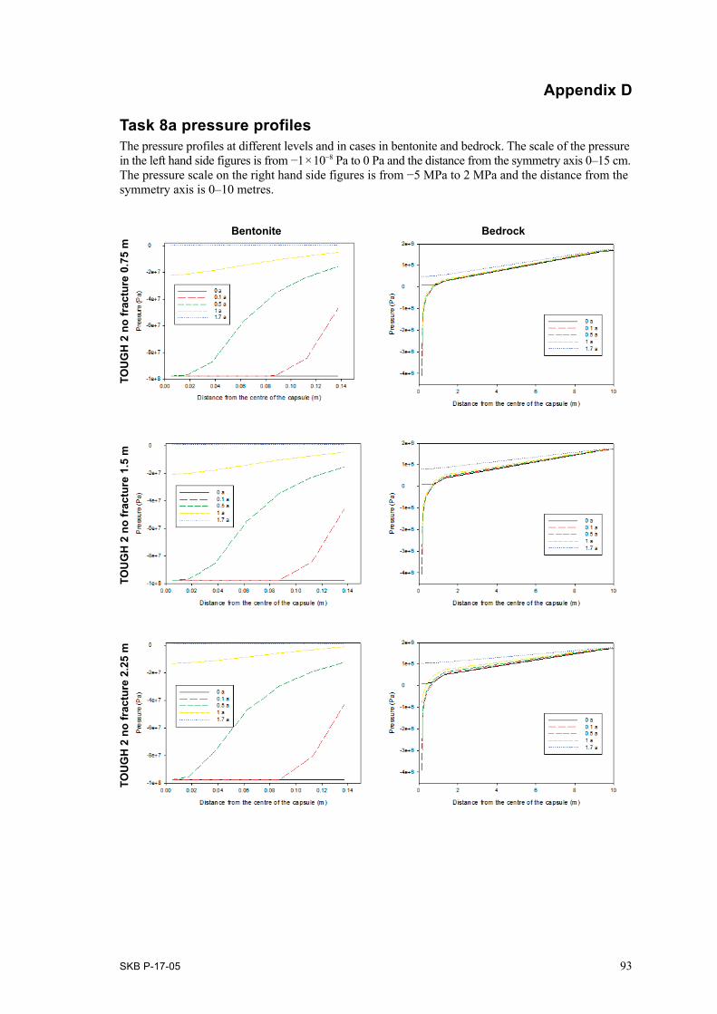
SKB P-17-05 93

Appendix D

Task 8a pressure profilesThe pressure profiles at different levels and in cases in bentonite and bedrock. The scale of the pressure in the left hand side figures is from −1 × 10−8 Pa to 0 Pa and the distance from the symmetry axis 0–15 cm. The pressure scale on the right hand side figures is from −5 MPa to 2 MPa and the distance from the symmetry axis is 0–10 metres.

TOU

GH

2 n

o fr

actu

re 0

.75

mTO

UG

H 2

no

frac

ture

1.5

mTO

UG

H 2

no

frac

ture

2.2

5 m

BedrockBentonite

94 SKB P-17-05

TOU

GH

2 f

ract

ure

0.75

mTO

UG

H 2

fra

ctur

e 1.

5 m

TOU

GH

2 f

ract

ure

2.25

mBedrockBentonite

SKB P-17-05 95

CO

MSO

L n

o fr

actu

re 0

.75

mC

OM

SOL

no

frac

ture

1.5

mC

OM

SOL

no

frac

ture

2.2

5 m

BedrockBentonite

96 SKB P-17-05

Bentonite BedrockC

OM

SOL

frac

ture

0.7

5 m

CO

MSO

L fr

actu

re 1

.5 m

CO

MSO

L fr

actu

re 2

.25

m

SKB P-17-05 97

Appendix E

Task 8b pressure and saturation profiles0

year

0.1

year

0.5

year

1 ye

ar

98 SKB P-17-05

0 ye

ar0.

1 ye

ar0.

5 ye

ar1

year

SKB P-17-05 99

Appendix F

Comparing the wetting model to the water uptake testThe objective of the comparison of the wetting model and the water uptake test is to make sure that the wetting model works reasonably accurately. The wetting model referred here to is the wetting model in subtasks c and d with the exactly same equations, mesh and solvers that were used in the subtasks. Although the geometries of the experiment and the models differ slightly (the 5 mm filter in the test is not included in the model), it is important to test the real model directly instead of creating a new one to build confidence in the subtask c and d models.

Experimental setupA block of similar bentonite that is used in BRIE is put in to metallic cylinder with 15 cm radius and 0.1 m height. A vertical smaller cylinder of 2 cm radius is put at the centre of the larger cylinder. A 5 mm thick filter covers the inner wall of the larger cylinder. The space between the filter and the small cylinder is filled with bentonite (1 mm installation cap between bentonite and the filter).

The total porosity of bentonite is 0.44 and initial dry density 1587 kg/m3. The initial saturation is 0.42 (11.75 % water content).

The bentonite block is allowed to wet through the filter and the water uptake, the relative humidities and pressures are monitored. Also, chemical analysis is done.

Model setupA cylinder with 15 cm radius and 20 cm height of the bentonite in the subtask 8d model is isolated in the model at a position where the mesh in bentonite is the coarsest. The initial pressure in bentonite is set to −67 MPa (corresponds to the initial water content in the experiment with the subtask c and d parameterization) and the radial boundary is set to air pressure (0.1 MPa). The top and bottom bounda-ries are no flow boundaries. The wetting of bentonite is computed using the subtask d parameters, mesh and solvers.

ResultsA comparison of the model and the experimental water uptakes is presented in Figure F-1. The saturation profiles at 107 and 203 days are illustrated in Figure F-2. The relative humidity sensor readings of the experiment are compared to the model values in Figure F-3.

Discussion and conclusionsAlthough the differences in the geometries of the experiment and the model are evident, the water uptake graph shows very good agreement between the water uptake test and the subtask c and d wetting models. The initial relative humidity shows the most significant difference, which is a result of using the parameterisation optimized for an initial water content that is not the uptake test initial water content. In other words, the initial relative humidity and the initial saturation do not match in the parameterisation.

100 SKB P-17-05

Figure F-1. Water uptake of the model and the experiment. Despite the slightly different geometries, the results almost coincide.

Figure F-2. Saturation profiles of the model and the experiment at 107 and 203 days.

SKB P-17-05 101

Figure F-3. Relative humidity sensor data from the experiment (zigzag) and corresponding model results (plain lines). The initial relative humidities differ due to the usage of wetting model optimised for different initial water content than in the experiment.