modelling spatial variations in household … · modelling spatial variations in household...
TRANSCRIPT

MODELLING SPATIAL VARIATIONS IN
HOUSEHOLD DISPOSABLE INCOME WITH GEOGRAPHICALLY WEIGHTED REGRESSION
Enero 2007 nº 15
Coro Chasco Yrigoyen Isabel García Rodríguez
José Vicéns Otero
The purpose of this paper is to analyze the spatially varying impacts of some classical regressors on per capita household income in Spanish provinces. The authors model this distribution following both a traditional global regression and a local analysis with Geographically Weighted Regression (GWR). Several specifications are compared, being the adaptive bisquare weighting function the more efficient in terms of goodness-of- fit. We test for global and local spatial instability using some F-tests and other statistical measures. We find some evidence of spatial instability in the distribution of this variable in relation to some explanatory variables, which cannot be totally solved by spatial dependence specifications. GWR has revealed as a better specification to model per capita household income. It highlights some facets of the relationship completely hidden in the global results and forces us to ask about questions we would otherwise not have asked. Moreover, the application of GWR can also be of help to further exercises of micro-data spatial prediction.

Modeling spatial variations in household disposable income with GWR __________________________________________________________________________________________
Instituto L.R. Klein – Centro Gauss. U.A.M. D.T. nº 15. February 2006
2
Edita: Instituto L.R. Klein – Centro Gauss Facultad de CC.EE. y EE. Universidad Autónoma de Madrid 28049 Madrid Teléfono y Fax: 91 4974191 Correo electrónico: [email protected] Página Web: www.uam.es/klein/gauss ISSN 1696-5035 Depósito Legal: M-30165-2003 © Todos los derechos reservados. Queda prohibida la reproducción total o parcial de esta publicación sin la previa autorización escrita del editor.
Modeling spatial variations in household disposable income with GWR __________________________________________________________________________________________
Instituto L.R. Klein – Centro Gauss. U.A.M. D.T. nº 15. February 2006
3
MODELING SPATIAL VARIATIONS IN HOUSEHOLD DISPOSABLE
INCOME WITH GEOGRAPHICALLY WEIGHTED REGRESSION1
Coro Chasco Yrigoyen Universidad Autónoma de Madrid
email: [email protected]
Isabel García Rodríguez Universidad Autónoma de Madrid
email: [email protected]
José Vicéns Otero Universidad Autónoma de Madrid
email: [email protected]
ABSTRACT The purpose of this paper is to analyze the spatially varying impacts of some classical regressors on per capita household income in Spanish provinces. The authors model this distribution following both a traditional global regression and a local analysis with Geographically Weighted Regression (GWR). Several specifications are compared, being the adaptive bisquare weighting function the more efficient in terms of goodness-of-fit. We test for global and local spatial instability using some F-tests and other statistical measures. We find some evidence of spatial instability in the distribution of this variable in relation to some explanatory variables, which cannot be totally solved by spatial dependence specifications. GWR has revealed as a better specification to model per capita household income. It highlights some facets of the relationship completely hidden in the global results and forces us to ask about questions we would otherwise not have asked. Moreover, the application of GWR can also be of help to further exercises of micro-data spatial prediction. Key words: Geographically Weighted Regression (GWR), spatial non-stationarity, spatial prediction, income, Spanish provinces. JEL Classification: C21, C51, C53, R12
1 Previous versions of this paper were presented at the III EUREAL (European Union Regional Economics Applications Laboratory) Workshop (University of Glasgow, UK, September 28-30, 2006), II Seminar “Jean Paelinck” on Spatial Econometrics (Universidad de Zaragoza, Spain, October 27-28, 2006) and at the Seminarios Klein (Universidad Autónoma de Madrid, December 14, 2006). We would like to thank Julie Le Gallo, Yiannis Kamarianakis , Vicente Royuela, Miguel Ángel Márquez, Esteban Fernández and the other participants of these meetings for their valuable comments, as well as Roger Bivand for his help with the use of the R software. The authors show gratitude to “la Caixa” for having sponsored the spatial prediction of household income in Spanish municipalities since 1996. Coro Chasco acknowledges financial support from the Spanish Ministry of Education and Science SEJ2006-02328/ECON. The usual disclaimers apply.
Modeling spatial variations in household disposable income with GWR __________________________________________________________________________________________
Instituto L.R. Klein – Centro Gauss. U.A.M. D.T. nº 15. February 2006
4
INTRODUCTION In regional science, the use of linear regression as an analytical technique has been long widely generalized. However, the explicit incorporation of “space” or “location” has not been that commonly considered. In this context, there has been recently a surge in econometric work focusing on the inclusion of spatial effects in econometric models. One strand of this literature has developed several approaches to incorporate the spatial non-stability. For a specific model, the assumption of stationarity or structural stability over space has been recognized highly unrealistic, accepting the possibility that parameters may vary over the study area. Several methods deal with this issue. Spatial analysis of variance (Griffith 1978, 1992) and models with structural change (Anselin 1988, 1990) are good examples of methods accounting for discrete spatial regimes, whilst the spatial expansion model (Casetti 1972, 1986) and the spatial adaptative filtering (Foster and Gorr 1986, Gorr and Olligschlaeger 1994) concern mostly about continuous variation over space. Getis and Ord (1992) and Openshaw (1993) study local patterns of association (hot spots) and local instabilities. Locally weighted regression method and kernel regression method (Cleveland 1979, Casetti 1982) focus mainly on the fit of a regression surface to data, using a weighting system that depends on the location of the independent variables. Along this line of thinking, in the spatial econometrics literature, McMillen (1996) and McMillen and McDonald (1997) introduced nonparametric locally linear regression in models where the cases are geographical location and Brunsdon et al. (1996) labelled them as “Geographically Weighted Regression” (GWR). Hence, GWR produces locally linear regression estimates for every point in space. For this purpose, weighted least squares methodology is used, with weights based on the distances between observations i and all the others in the sample. GWR allows the exploration of the variation of the parameters as well as the testing of the significance of this variation. This methodology has recently received intensive attention (Brunsdon et al. 1996, 1999; Fotheringham and Brunsdon (1999); Fotheringham et al. 1997, 1998, 2002; Leung et al. 2000a; Huang and Leung 2002, Paez et al. 2002(a,b); Yu and Wu 2004, to name a few). Furthermore, LeSage (1999) introduces a Bayesian approach (BGWR) that subsumes GWR as a special case of a much broader class of spatial econometric models. This methodology overcomes outliers and weak data problems using robust estimates and permitting the

Modeling spatial variations in household disposable income with GWR __________________________________________________________________________________________
Instituto L.R. Klein – Centro Gauss. U.A.M. D.T. nº 15. February 2006
5
introduction of subjective prior information, improving at the same time the inference procedure. Some example of the application of GWR methodology can be found in Fotheringham et al. (2000), Huang and Leung (2002), Yu and Wu (2004), Mennis and Jordan (2005), Kentor and Miller (2004), Eckey et al. (2005), Bivand and Brunstad (2005), Yu (2006), etc. The purpose of this paper is to analyze the spatially varying impacts of some classical regressors on per capita household disposable income of Spanish provinces. This variable, which is considered a good indicator of regional welfare, has frequently been estimated for microterritorial units (e.g. municipalities) from aggregate data (e.g. provinces, regions). In some countries with scarce availability of economic macromagnitudes for micro-level units, such as Spain or Portugal, there is an interesting literature in what are called “indirect methods of income estimation” (see Chasco 2003, pp. 178 for a broad revision). These are particular cases of the ecological inference topic, which consists in making inferences about individual behavior drawn from data about aggregates. Clearly, observations at an aggregated level of analysis do not necessarily provide useful information about lower levels of analysis, particularly when spatial heterogeneity (non-stationarity) is present (Peeters and Chasco 20062). For that reason, we propose to test spatial variation of the determinants of household disposable income across Spanish provinces (nut3). If this effect was present, it should be considered, particularly in future ecological inferences of municipal income. Therefore, we model the provincial household income distribution following a basic global regression, which was also re-specified to take into account spatial effects. We found clear evidence of spatial instability in the distribution of the residuals that could not be totally solved by global specifications. Since spatial autocorrelation in the residuals may be implied by some kind of spatial heterogeneity not always correctly modeled by spatial dependence specifications, we propose the re-specification of the basic model using GWR. The outline of the paper is as follows. In section 2, we present a theoretical framework for GWR. Section 3 offers the empirical framework: data, econometric results and spatial non-stationarity tests are displayed. Finally, section 4 concludes.
2 In this paper, the authors demonstrated the existence of spatial instability in per capita GDP across Spanish regions (nut2), as well of varying relations in the explanatory variables of a production-function Cobb-Douglas model.

Modeling spatial variations in household disposable income with GWR __________________________________________________________________________________________
Instituto L.R. Klein – Centro Gauss. U.A.M. D.T. nº 15. February 2006
6
I.- GEOGRAPHICALLY WEIGHTED REGRESSIONS (GWR)
Specification
The technique of linear regression estimates a parameter β that links the independent variables to the dependent variable. However, when this technique is applied to spatial data, some issues concerning the stability of these parameters over the space come out/arise. There have been several approaches to incorporate this spatial non-stability in the model. One of them, developed by Brundston et al. (1996), has been labelled Geographically Weighted Regressions (GWR). It is a non-parametric model of spatial drift that relies on a sequence of locally linear regressions to produce estimates for every point in space by using a sub-sample of data information from nearby observations. That is to say, this technique allows the modelling of relationships that vary over space by introducing distance-based weights to provide estimates of kiβ for each variable k and each geographical location i.
An ordinary linear regression model can be expressed by:
01=
= + +∑β βM
i k ki ik
y x u
(1)
where yi, 1 2=i , ,...,N are the observation of the dependent variable y,
kβ ( 1 2=k , ,...,M ) represents the regression coefficients, xki is the ith value of xk and ui are the independent normally distributed error terms with zero mean and constant variance.
In matrix notation:
01
m
k kk
y x uβ β=
= + +∑
(2)
with y as vector of the dependent variable, xk as vector of the kth independent variable and u as vector of the error term. In geographically weighted regression the global regression coefficients are replace by local parameters:
01=
= + ⋅ +∑β βm
i i ki ki ik
y x u
(3)
Modeling spatial variations in household disposable income with GWR __________________________________________________________________________________________
Instituto L.R. Klein – Centro Gauss. U.A.M. D.T. nº 15. February 2006
7
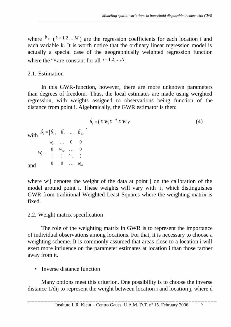
where kiβ ( 1 2=k , ,...,M ) are the regression coefficients for each location i and each variable k. It is worth notice that the ordinary linear regression model is actually a special case of the geographically weighted regression function where the kiβ are constant for all 1 2=i , ,...,N . 2.1. Estimation In this GWR-function, however, there are more unknown parameters than degrees of freedom. Thus, the local estimates are made using weighted regression, with weights assigned to observations being function of the distance from point i. Algebraically, the GWR estimator is then:
( )-1ˆi i iX W X X W yβ ′ ′= (4)
with ( )0 1ˆ ˆ ˆ ˆ...i i i iMβ β β β ′=
and
1
2
0 0
0 0
0 0
i
ii
iN
w
wW
w
… … =
…
M M O M
where wij denotes the weight of the data at point j on the calibration of the model around point i. These weights will vary with i, which distinguishes GWR from traditional Weighted Least Squares where the weighting matrix is fixed. 2.2. Weight matrix specification The role of the weighting matrix in GWR is to represent the importance of individual observations among locations. For that, it is necessary to choose a weighting scheme. It is commonly assumed that areas close to a location i will exert more influence on the parameter estimates at location i than those farther away from it.
• Inverse distance function Many options meet this criterion. One possibility is to choose the inverse distance 1/dij to represent the weight between location i and location j, where d
Modeling spatial variations in household disposable income with GWR __________________________________________________________________________________________
Instituto L.R. Klein – Centro Gauss. U.A.M. D.T. nº 15. February 2006
8
is the Euclidean distance ( )22( , ) ik jkkd i j x x= −∑ between the location i and j.
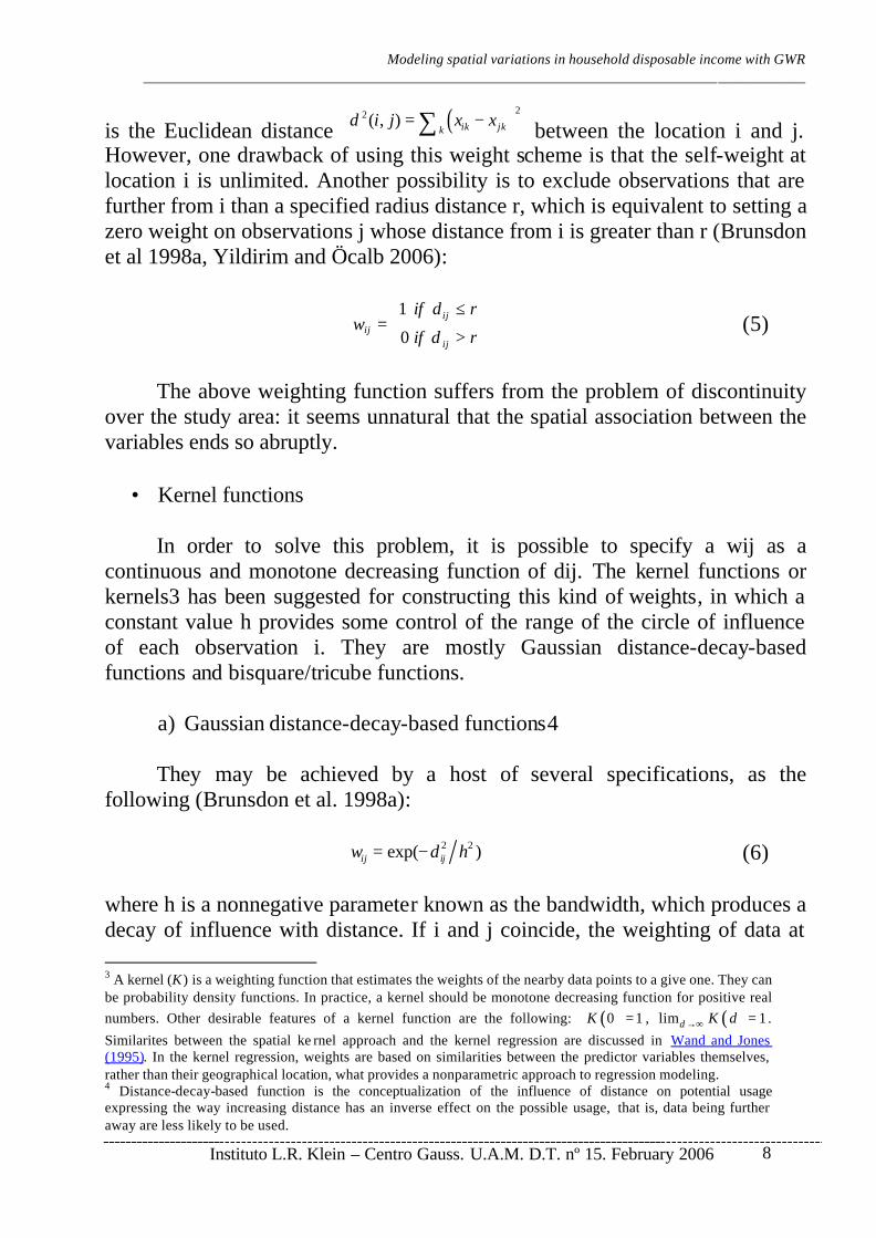
However, one drawback of using this weight scheme is that the self-weight at location i is unlimited. Another possibility is to exclude observations that are further from i than a specified radius distance r, which is equivalent to setting a zero weight on observations j whose distance from i is greater than r (Brunsdon et al 1998a, Yildirim and Öcalb 2006):
>
≤=
rdif
rdifw
ij
ijij 0
1
(5)
The above weighting function suffers from the problem of discontinuity over the study area: it seems unnatural that the spatial association between the variables ends so abruptly.
• Kernel functions In order to solve this problem, it is possible to specify a wij as a continuous and monotone decreasing function of dij. The kernel functions or kernels3 has been suggested for constructing this kind of weights, in which a constant value h provides some control of the range of the circle of influence of each observation i. They are mostly Gaussian distance-decay-based functions and bisquare/tricube functions.
a) Gaussian distance-decay-based functions4 They may be achieved by a host of several specifications, as the
following (Brunsdon et al. 1998a):
2 2exp( )ij ijw d h= − (6) where h is a nonnegative parameter known as the bandwidth, which produces a decay of influence with distance. If i and j coincide, the weighting of data at 3 A kernel (K ) is a weighting function that estimates the weights of the nearby data points to a give one. They can be probability density functions. In practice, a kernel should be monotone decreasing function for positive real numbers. Other desirable features of a kernel function are the following: ( )0 1K = , ( )lim 1d K d→∞ = .
Similarites between the spatial ke rnel approach and the kernel regression are discussed in Wand and Jones (1995). In the kernel regression, weights are based on similarities between the predictor variables themselves, rather than their geographical location, what provides a nonparametric approach to regression modeling. 4 Distance-decay-based function is the conceptualization of the influence of distance on potential usage expressing the way increasing distance has an inverse effect on the possible usage, that is, data being further away are less likely to be used.

Modeling spatial variations in household disposable income with GWR __________________________________________________________________________________________
Instituto L.R. Klein – Centro Gauss. U.A.M. D.T. nº 15. February 2006
9
that point will be the unity. Changing the bandwidth results in a different exponential decay profile, which in turn produces estimates that vary more or less rapidly over space. The weighting of other data will decrease according to a Gaussian curve as the distance between i and j increases. For data a long way from i the weighting will fall to virtually zero, effectively excluding these observations from the estimation of parameters for location i. This function is the most commonly used (Huang and Leung 2002) and
has received many other specifications, e.g. exp( )= −ij ijw d h (Brundson et al. 1996) or
2exp( )= − ⋅ij ijw h d (Fotheringham et al. (1997, 2001). Still another approach is to rely on the Gaussian function φ (Le Sage
2004) can be ( )i iW d hφ σ= , where φ denotes the standard normal density and σ represents the standard deviation of the distance vector di, which represents a vector of distances between observation i and all other sample data observations.
b) Bisquare and tricube weighting schemes. Specifically, the formal expression of the bisquare weighting function is the following (Brunsdon et al 1998a, Bivand and Brunstad 2005):
( )22
1 / , if
0 , otherwise
ij ijij
d h d hw
− < =
(7)
where h is the maximum -constant- distance for non-zero weights. As h tends to infinity, weights tend to the total sample (N) for all pairs of points so that the estimated parameters become uniform and GWR becomes equivalent to Ordinary Least Squares (OLS)5. Conversely, as the bandwidth gets smaller, the estimates of the parameters will increasingly depend on observations close to i and hence will have increased variance. In each case, the constant value h provides some control of the range of the circle of influence of each observation i.
5 One of the advantages of these functions is that they allow saving time in computation processes. In effect, if the number of observations for which weighting is non-zero is significantly smaller than N, then the computation overhead of (4) can be reduced by treating the problem as though it were only applied to the non-zero weighted observation (Brunsdon et al. 1998a).

Modeling spatial variations in household disposable income with GWR __________________________________________________________________________________________
Instituto L.R. Klein – Centro Gauss. U.A.M. D.T. nº 15. February 2006
10
On its side, the tricube kernel function, proposed by McMillen (1996), is
specified in a similar way: ( ) ( )
331 / , if Iij ij iw d h d h = − < , and 0 otherwise.
c) Adaptive weighting schemes.
In general, all the spatial kernel functions fall within two categories, i.e., fixed or adaptive spatial kernel functions. In a fixed spatial kernel function, one optimum spatial kernel (represented by the spatial bandwidth) is determined and applied uniformly across the study area. Such approach, however, suffer from the potential problem that in some parts of the region, where data are sparse, the local regressions might be based on relatively few data points. As pointed out by Paez et al. (2002a, b) and Fotheringham et al. (2002), fixed spatial kernels may produce large local estimation variance in areas where data are sparse, which might exaggerate the degree of non-stationarity present. They also might mask subtle spatial non-stationarity at where data are dense. To offset this problem, spatially adaptive weighting functions can be incorporated into GWR. These functions would have different bandwidths (distances), expressing the number or proportion of observations to retain within the weighting kernel “window”, irrespective of distance: on the one hand, relatively small bandwidths in areas where the data points are densely distributed and on the other hand, relatively large bandwidths where the data points are sparsely distributed. In other words, they are able to adapt themselves in size to variations in the density of the data so that the kernels have larger bandwidths where the data are sparse and have smaller ones where the data are plentiful. In these cases, the bandwidth is adaptive in size and acts to ensure that the same number of non-zero weights is used for each regression point in the analysis. For example, the adaptive bisquare weighting function is the following:
( )22
1 / , if
0 , otherwise
ij i ij iij
d h d hw
− < =
(8)
where hi represents the different bandwidths (distances), which express the number or proportion of observations to consider in the estimation of the regression at location i.

Modeling spatial variations in household disposable income with GWR __________________________________________________________________________________________
Instituto L.R. Klein – Centro Gauss. U.A.M. D.T. nº 15. February 2006
11
2.3. Bandwidth selection The problem is now therefore how to select the optimal bandwidth. If we have strong theoretically based prior beliefs about the value of h in a given situation, then it is reasonable to make use of them. However, that information is usually missing. Anyway, since different h will result in different weight matrices Wi, the estimated parameters of GWR are not unique. The best h can be chosen using the least squares cross-validation method (Cleve land 1979; Fotheringham et al. 2002). Suppose that the predicted value of yi from GWR is denoted as a functions of h by ˆ ( )∗
iy h . The sum of squared errors may then be written as:
2ˆRSS( ) ( )∗ = − ∑ i i
i
h y y h (9)
A logical choice would be to find h minimizing this equation. However, when h is very large the weighting of all locations except for i itself become negligible ( 0→ijw ) and the fitted
values at location i will tend to the actual values ( ˆ ( )∗ →i iy h y ). This suggests that an unmodified least squares automatic choice of h would always lead to → ∞h , or possibly result in computational errors. This problem can be avoided if, for each i, a GWR estimate of yi is obtained by omitting the ith observation from the model. If the modified GWR estimate of yi is denoted by ˆ ( )∗
≠ iy h then the cross-validates sum of squared errors is denoted by:
2ˆCVRSS( ) ( )∗
≠ = − ∑ i ii
h y y h (10)
Choosing h to minimize this equation provides a method for choosing h automatically that does not suffer from the problems encountered by working with RSS(h). Thus, when h becomes very large, the model is calibrated only on samples near to i and not at i itself (Brunsdon et al. 1998b). For the specific case of the adaptive spatial kernels and the tri-cube weighting function, we would compute a value for h (or q) denoting the number of nearest neighbors beyond which we impose zero weights. The score function would be evaluated using alternative values of q to find a value that minimizes the function6. 1. SPATIAL INSTABILITY IN THE PER CAPITA DISPOSABLE INCOME
DISTRIBUTION OF SPANISH PROVINCES This section examines the spatial distribution of the per capita disposable income of Spanish provinces. This case is well known and has been tackled by many authors (Cuadrado et al. 1998, Vicéns and Chasco 1998, Garrido 2002, Alcaide and Alcaide 2005 between others). Thus, our objective is to use this case for applying the methodology that we develop in the previous section. If some kind of continuous spatial instability is found across Spanish provinces, this
6 Another estimation method for h consists in minimizing the goodness-of-fit statistics, the corrected Akaike Information Criterion or AICc (Hurvich et al. 1998; Fotheringham et al. 2002).

Modeling spatial variations in household disposable income with GWR __________________________________________________________________________________________
Instituto L.R. Klein – Centro Gauss. U.A.M. D.T. nº 15. February 2006
12
should be taken into account in some studies, e.g. spatial prediction of municipal income (Alañón 2001, Chasco 2003, Chasco and López 2004, Cravo et al. 2004). In the first subsection, we present the data that we have used. In the second, we specify a basic global model, which is estimated by ordinary least squares; this model is tested for spatial autocorrelation and respecified using different spatial dependence models. In the third subsection, we go deeper into the spatial structure of the data in search of symptoms of spatial instability and estimate a GWR model using different weighting schemes. Next, we test for spatial non-stationarity in the relationship between income and the covariates. Finally, we propose a final spatial regimes model, with different regimes for each non-constant parameter, which fits better than the other models and leads to white noise errors. 4.1. Data The data employed in the analysis come from the Spanish Office for Statistics (INE) databank. The sample includes the 50 Spanish provinces (the Autonomous Cities of Ceuta and Melilla have been excluded). The INE provides provincial data of household disposable income in the Regional Accounts for the period 2000-2004. The series for 2004 shows (Figure 1) that the highest per capita GDP is observed mainly in the Northeast provinces, which forms a big quadrant determined by the Bask Country, Navarre, La Rioja and Catalonia, including Madrid and the Balearics (above 13,800 euros per capita). On the other end of the distribution, the lowest per capita income is registered in Southern provinces, mainly Extremadura, Andalusia and Castile-La Mancha (below 10,700 euros per capita). In this paper, we want to test the existence of continuous spatial instability of the parameters in a model of per capita household income of Spanish provinces for the year 2004. In spatial prediction, the main aim is to find explanatory variables that exert a good correlation with the endogenous, though it is not “caused” by them in a Granger sense. The explanatory variables must be available not only for the provincial leve l but also for the municipal one. This imposes an important restriction since some “a priori” good explanatory variables cannot be used or must be proxied. For that purpose, it is preferable to select as many regressors as possible and avoid multicollinearity with principal components analysis. We have specified the basic model shown in “la Caixa” (2005). In this book, the authors present a spatial prediction exercise of municipal income data from the provincial series. This kind of estimation can be criticized because it estimates only one –national average- coefficient for each explanatory variable, which is applied afterwards to estimate the whole set of Spanish municipalities. If spatial instability is proved in the provincial (aggregate) model of household income, a GWR approach could improve these spatial prediction exercises as it allows for estimating one different coefficient for each province.
Figure 1. Per capita household disposable income of Spanish provinces for 2004

Modeling spatial variations in household disposable income with GWR __________________________________________________________________________________________
Instituto L.R. Klein – Centro Gauss. U.A.M. D.T. nº 15. February 2006
13
alaalaalaalaalaalaalaalaalaalaalaalaalaalaalaalaalaalaalaalaalaalaalaalaalaalaalaalaalaalaalaalaalaalaalaalaalaalaalaalaalaalaalaalaalaalaalaalaala
burburburburburburburburburburburburburburburburburburburburburburburburburburburburburburburburburburburburburburburburburburburburburburburburburpalpalpalpalpalpalpalpalpalpalpalpalpalpalpalpalpalpalpalpalpalpalpalpalpalpalpalpalpalpalpalpalpalpalpalpalpalpalpalpalpalpalpalpalpalpalpalpalpal
cancancancancancancancancancancancancancancancancancancancancancancancancancancancancancancancancancancancancancancancancancancancancancancancancan
rioriorioriorioriorioriorioriorioriorioriorioriorioriorioriorioriorioriorioriorioriorioriorioriorioriorioriorioriorioriorioriorioriorioriorioriorio
vizvizvizvizvizvizvizvizvizvizvizvizvizvizvizvizvizvizvizvizvizvizvizvizvizvizvizvizvizvizvizvizvizvizvizvizvizvizvizvizvizvizvizvizvizvizvizvizvizguiguiguiguiguiguiguiguiguiguiguiguiguiguiguiguiguiguiguiguiguiguiguiguiguiguiguiguiguiguiguiguiguiguiguiguiguiguiguiguiguiguiguiguiguiguiguiguigui
segsegsegsegsegsegsegsegsegsegsegsegsegsegsegsegsegsegsegsegsegsegsegsegsegsegsegsegsegsegsegsegsegsegsegsegsegsegsegsegsegsegsegsegsegsegsegsegseg
navnavnavnavnavnavnavnavnavnavnavnavnavnavnavnavnavnavnavnavnavnavnavnavnavnavnavnavnavnavnavnavnavnavnavnavnavnavnavnavnavnavnavnavnavnavnavnavnav
cadcadcadcadcadcadcadcadcadcadcadcadcadcadcadcadcadcadcadcadcadcadcadcadcadcadcadcadcadcadcadcadcadcadcadcadcadcadcadcadcadcadcadcadcadcadcadcadcad
sevsevsevsevsevsevsevsevsevsevsevsevsevsevsevsevsevsevsevsevsevsevsevsevsevsevsevsevsevsevsevsevsevsevsevsevsevsevsevsevsevsevsevsevsevsevsevsevsev
almalmalmalmalmalmalmalmalmalmalmalmalmalmalmalmalmalmalmalmalmalmalmalmalmalmalmalmalmalmalmalmalmalmalmalmalmalmalmalmalmalmalmalmalmalmalmalmalmmurmurmurmurmurmurmurmurmurmurmurmurmurmurmurmurmurmurmurmurmurmurmurmurmurmurmurmurmurmurmurmurmurmurmurmurmurmurmurmurmurmurmurmurmurmurmurmurmur
alialialialialialialialialialialialialialialialialialialialialialialialialialialialialialialialialialialialialialialialialialialialialialialialiali
valvalvalvalvalvalvalvalvalvalvalvalvalvalvalvalvalvalvalvalvalvalvalvalvalvalvalvalvalvalvalvalvalvalvalvalvalvalvalvalvalvalvalvalvalvalvalvalval
cascascascascascascascascascascascascascascascascascascascascascascascascascascascascascascascascascascascascascascascascascascascascascascascascas
tartartartartartartartartartartartartartartartartartartartartartartartartartartartartartartartartartartartartartartartartartartartartartartartartarbarbarbarbarbarbarbarbarbarbarbarbarbarbarbarbarbarbarbarbarbarbarbarbarbarbarbarbarbarbarbarbarbarbarbarbarbarbarbarbarbarbarbarbarbarbarbarbarbar
balbalbalbalbalbalbalbalbalbalbalbalbalbalbalbalbalbalbalbalbalbalbalbalbalbalbalbalbalbalbalbalbalbalbalbalbalbalbalbalbalbalbalbalbalbalbalbalbal
girgirgirgirgirgirgirgirgirgirgirgirgirgirgirgirgirgirgirgirgirgirgirgirgirgirgirgirgirgirgirgirgirgirgirgirgirgirgirgirgirgirgirgirgirgirgirgirgir
albalbalbalbalbalbalbalbalbalbalbalbalbalbalbalbalbalbalbalbalbalbalbalbalbalbalbalbalbalbalbalbalbalbalbalbalbalbalbalbalbalbalbalbalbalbalbalbalb
malmalmalmalmalmalmalmalmalmalmalmalmalmalmalmalmalmalmalmalmalmalmalmalmalmalmalmalmalmalmalmalmalmalmalmalmalmalmalmalmalmalmalmalmalmalmalmalmal
gragragragragragragragragragragragragragragragragragragragragragragragragragragragragragragragragragragragragragragragragragragragragragragragragra
zarzarzarzarzarzarzarzarzarzarzarzarzarzarzarzarzarzarzarzarzarzarzarzarzarzarzarzarzarzarzarzarzarzarzarzarzarzarzarzarzarzarzarzarzarzarzarzarzar
huehuehuehuehuehuehuehuehuehuehuehuehuehuehuehuehuehuehuehuehuehuehuehuehuehuehuehuehuehuehuehuehuehuehuehuehuehuehuehuehuehuehuehuehuehuehuehuehue
madmadmadmadmadmadmadmadmadmadmadmadmadmadmadmadmadmadmadmadmadmadmadmadmadmadmadmadmadmadmadmadmadmadmadmadmadmadmadmadmadmadmadmadmadmadmadmadmadguaguaguaguaguaguaguaguaguaguaguaguaguaguaguaguaguaguaguaguaguaguaguaguaguaguaguaguaguaguaguaguaguaguaguaguaguaguaguaguaguaguaguaguaguaguaguaguagua
ponponponponponponponponponponponponponponponponponponponponponponponponponponponponponponponponponponponponponponponponponponponponponponponponpon
salsalsalsalsalsalsalsalsalsalsalsalsalsalsalsalsalsalsalsalsalsalsalsalsalsalsalsalsalsalsalsalsalsalsalsalsalsalsalsalsalsalsalsalsalsalsalsalsal
caccaccaccaccaccaccaccaccaccaccaccaccaccaccaccaccaccaccaccaccaccaccaccaccaccaccaccaccaccaccaccaccaccaccaccaccaccaccaccaccaccaccaccaccaccaccaccaccac
badbadbadbadbadbadbadbadbadbadbadbadbadbadbadbadbadbadbadbadbadbadbadbadbadbadbadbadbadbadbadbadbadbadbadbadbadbadbadbadbadbadbadbadbadbadbadbadbad
huehuehuehuehuehuehuehuehuehuehuehuehuehuehuehuehuehuehuehuehuehuehuehuehuehuehuehuehuehuehuehuehuehuehuehuehuehuehuehuehuehuehuehuehuehuehuehuehue
palpalpalpalpalpalpalpalpalpalpalpalpalpalpalpalpalpalpalpalpalpalpalpalpalpalpalpalpalpalpalpalpalpalpalpalpalpalpalpalpalpalpalpalpalpalpalpalpalscrscrscrscrscrscrscrscrscrscrscrscrscrscrscrscrscrscrscrscrscrscrscrscrscrscrscrscrscrscrscrscrscrscrscrscrscrscrscrscrscrscrscrscrscrscrscrscrscr
acoacoacoacoacoacoacoacoacoacoacoacoacoacoacoacoacoacoacoacoacoacoacoacoacoacoacoacoacoacoacoacoacoacoacoacoacoacoacoacoacoacoacoacoacoacoacoacoaco
aviaviaviaviaviaviaviaviaviaviaviaviaviaviaviaviaviaviaviaviaviaviaviaviaviaviaviaviaviaviaviaviaviaviaviaviaviaviaviaviaviaviaviaviaviaviaviaviavi
crecrecrecrecrecrecrecrecrecrecrecrecrecrecrecrecrecrecrecrecrecrecrecrecrecrecrecrecrecrecrecrecrecrecrecrecrecrecrecrecrecrecrecrecrecrecrecrecre
corcorcorcorcorcorcorcorcorcorcorcorcorcorcorcorcorcorcorcorcorcorcorcorcorcorcorcorcorcorcorcorcorcorcorcorcorcorcorcorcorcorcorcorcorcorcorcorcor
cuecuecuecuecuecuecuecuecuecuecuecuecuecuecuecuecuecuecuecuecuecuecuecuecuecuecuecuecuecuecuecuecuecuecuecuecuecuecuecuecuecuecuecuecuecuecuecuecue
jaejaejaejaejaejaejaejaejaejaejaejaejaejaejaejaejaejaejaejaejaejaejaejaejaejaejaejaejaejaejaejaejaejaejaejaejaejaejaejaejaejaejaejaejaejaejaejaejae
leoleoleoleoleoleoleoleoleoleoleoleoleoleoleoleoleoleoleoleoleoleoleoleoleoleoleoleoleoleoleoleoleoleoleoleoleoleoleoleoleoleoleoleoleoleoleoleoleollel lel lel lel lel lel lellellellellellellellel lel lel lel lel lel lel lel lel lel lel lel lel lel lel lel lel lel lel lel lellellellellellellellel lel lel lel lel lel lel lel le
lugluglugluglugluglugluglugluglugluglugluglugluglugluglugluglugluglugluglugluglugluglugluglugluglugluglugluglugluglugluglugluglugluglugluglugluglug
ourourourourourourourourourourourourourourourourourourourourourourourourourourourourourourourourourourourourourourourourourourourourourourourourour
astastastastastastastastastastastastastastastastastastastastastastastastastastastastastastastastastastastastastastastastastastastastastastastastast
sorsorsorsorsorsorsorsorsorsorsorsorsorsorsorsorsorsorsorsorsorsorsorsorsorsorsorsorsorsorsorsorsorsorsorsorsorsorsorsorsorsorsorsorsorsorsorsorsor
terterterterterterterterterterterterterterterterterterterterterterterterterterterterterterterterterterterterterterterterterterterterterterterterter
toltoltoltoltoltoltoltoltoltoltoltoltoltoltoltoltoltoltoltoltoltoltoltoltoltoltoltoltoltoltoltoltoltoltoltoltoltoltoltoltoltoltoltoltoltoltoltoltol
vallvallvallvallvallvallvallvallvallvallvallvallvallvallvallvallvallvallvallvallvallvallvallvallvallvallvallvallvallvallvallvallvallvallvallvallvallvallvallvallvallvallvallvallvallvallvallvallvallzamzamzamzamzamzamzamzamzamzamzamzamzamzamzamzamzamzamzamzamzamzamzamzamzamzamzamzamzamzamzamzamzamzamzamzamzamzamzamzamzamzamzamzamzamzamzamzamzam Income per capita(euros, 2004)
9,457 to 10,47010,470 to 11,89011,890 to 13,77013,770 to 16,257
Descriptive statistics:
Label Minimum Lwr quartile Median Upr quartile MaximumHousehold income per capita 9 10 11 13 16Provinces Badajoz (bad) Albacete Valencia Huesca
(hue)Álava
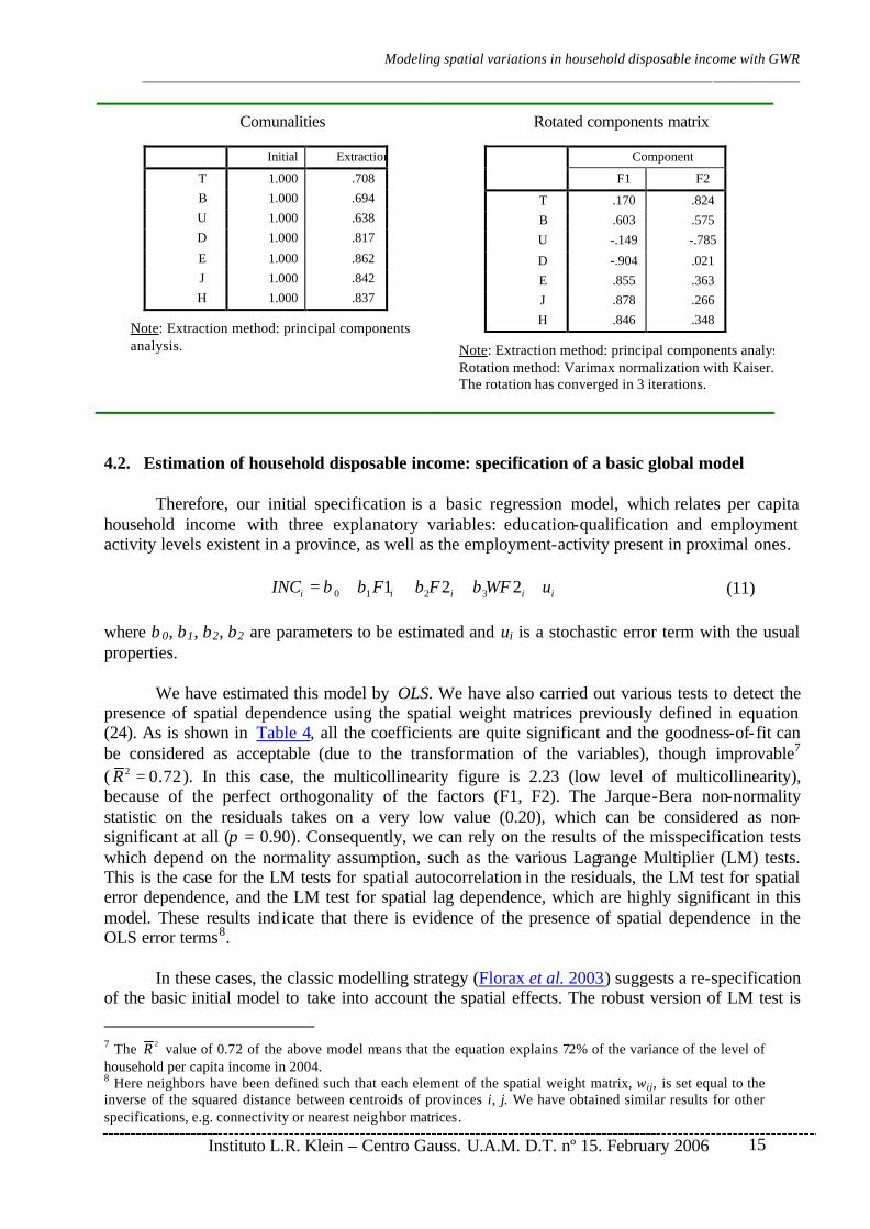
Source: INE 2007. The variable income per capita has been classified in the map with a method called “natural breaks”, which identifies breakpoints between classes using Jenks optimization (Jenks and Caspall 1971). This method is rather complex, but basically it minimizes the sum of the variance within each of the classes, finding groupings and patterns inherent in the data. First, we have grouped the original set of 7 explanatory variables into two factors using principal components analysis and Varimax rotation. These variables are the following (all rated by population): domestic telephone lines, broadband telephone lines, population with secondary and university degrees, population with qualified jobs, unemployment, average distance to the capital and commercial heads and average housing price. They are fully specified in Table 2. The use of principal components is clearly necessary since some of the explanatory variables are highly correlated each other. This is the case of average distance to the capital and commercial heads, which gets a Pearson correlation coefficient above 0.7 with three variables: population with secondary and university degrees, population with qualified jobs and average housing price. We find also very high correlation coefficients (above 0.8) between average housing price and two variables: population with secondary and university degrees and population with qualified jobs. Moreover, the latter are also correlated (Pearson above 0.7) with broadband telephone lines. The principal components analysis produces 2 factors with 77% of cumulative variance and communalities over 0,7 in all cases, except broadband lines and unemployment rate. The rotated factors can be interpreted as follows: factor 1 (F1) contains high scores of variables as secondary and university degrees, qualified jobs, housing price and average distance to capitals (negative), which are related to educated-qualified people that live in well-communicated provinces with higher housing price. Regarding factor 2 (F2), it is mainly based on telephone lines (domestic and broadband) and unemployment (negative), which are related to provinces with higher economic activity and lower unemployment rates. In Table 3, we present the communalities and the rotated factors matrix.
Modeling spatial variations in household disposable income with GWR __________________________________________________________________________________________
Instituto L.R. Klein – Centro Gauss. U.A.M. D.T. nº 15. February 2006
14
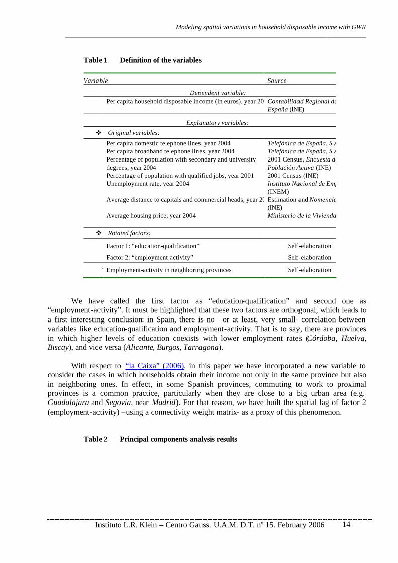
Table 1 Definition of the variables
Variable Source
Dependent variable: Per capita household disposable income (in euros), year 2004Contabilidad Regional de
España (INE)
Explanatory variables:
v Original variables:
Per capita domestic telephone lines, year 2004 Telefónica de España, S.A.Per capita broadband telephone lines, year 2004 Telefónica de España, S.A.Percentage of population with secondary and university degrees, year 2004
2001 Census, Encuesta de Población Activa (INE)
Percentage of population with qualified jobs, year 2001 2001 Census (INE) Unemployment rate, year 2004 Instituto Nacional de Empleo
(INEM) Average distance to capitals and commercial heads, year 2004Estimation and Nomenclator
(INE) Average housing price, year 2004 Ministerio de la Vivienda
v Rotated factors:
Factor 1: “education-qualification” Self-elaboration
Factor 2: “employment-activity” Self-elaboration
WF2Employment-activity in neighboring provinces Self-elaboration
We have called the first factor as “education-qualification” and second one as “employment-activity”. It must be highlighted that these two factors are orthogonal, which leads to a first interesting conclusion: in Spain, there is no –or at least, very small- correlation between variables like education-qualification and employment-activity. That is to say, there are provinces in which higher levels of education coexists with lower employment rates (Córdoba, Huelva, Biscay), and vice versa (Alicante, Burgos, Tarragona). With respect to “la Caixa” (2006), in this paper we have incorporated a new variable to consider the cases in which households obtain their income not only in the same province but also in neighboring ones. In effect, in some Spanish provinces, commuting to work to proximal provinces is a common practice, particularly when they are close to a big urban area (e.g. Guadalajara and Segovia, near Madrid). For that reason, we have built the spatial lag of factor 2 (employment-activity) –using a connectivity weight matrix- as a proxy of this phenomenon.
Table 2 Principal components analysis results
Modeling spatial variations in household disposable income with GWR __________________________________________________________________________________________
Instituto L.R. Klein – Centro Gauss. U.A.M. D.T. nº 15. February 2006
15
Comunalities
Initial Extraction
T 1.000 .708 B 1.000 .694 U 1.000 .638 D 1.000 .817
E 1.000 .862 J 1.000 .842 H 1.000 .837
Note: Extraction method: principal components analysis.
Rotated components matrix
Component
F1 F2
T .170 .824 B .603 .575 U -.149 -.785
D -.904 .021 E .855 .363 J .878 .266 H .846 .348
Note: Extraction method: principal components analysis. Rotation method: Varimax normalization with Kaiser. The rotation has converged in 3 iterations.
4.2. Estimation of household disposable income: specification of a basic global model Therefore, our initial specification is a basic regression model, which relates per capita household income with three explanatory variables: education-qualification and employment activity levels existent in a province, as well as the employment-activity present in proximal ones.
0 1 2 31 2 2i i i i iINC F F WF uβ β β β= + + + + (11) where β0, β1, β2, β2 are parameters to be estimated and ui is a stochastic error term with the usual properties. We have estimated this model by OLS. We have also carried out various tests to detect the presence of spatial dependence using the spatial weight matrices previously defined in equation (24). As is shown in Table 4, all the coefficients are quite significant and the goodness-of- fit can be considered as acceptable (due to the transformation of the variables), though improvable7 ( 2 0.72R = ). In this case, the multicollinearity figure is 2.23 (low level of multicollinearity), because of the perfect orthogonality of the factors (F1, F2). The Jarque-Bera non-normality statistic on the residuals takes on a very low value (0.20), which can be considered as non-significant at all (p = 0.90). Consequently, we can rely on the results of the misspecification tests which depend on the normality assumption, such as the various Lagrange Multiplier (LM) tests. This is the case for the LM tests for spatial autocorrelation in the residuals, the LM test for spatial error dependence, and the LM test for spatial lag dependence, which are highly significant in this model. These results ind icate that there is evidence of the presence of spatial dependence in the OLS error terms8. In these cases, the classic modelling strategy (Florax et al. 2003) suggests a re-specification of the basic initial model to take into account the spatial effects. The robust version of LM test is
7 The 2R value of 0.72 of the above model means that the equation explains 72% of the variance of the level of household per capita income in 2004. 8 Here neighbors have been defined such that each element of the spatial weight matrix, wij, is set equal to the inverse of the squared distance between centroids of provinces i, j. We have obtained similar results for other specifications, e.g. connectivity or nearest neighbor matrices.

Modeling spatial variations in household disposable income with GWR __________________________________________________________________________________________
Instituto L.R. Klein – Centro Gauss. U.A.M. D.T. nº 15. February 2006
16
only significant for the spatial lag dependence. We have tested different spatial dependence specifications, such as spatial lag, spatial cross-regressive, mixed spatial autoregressive cross-regressive models (see Anselin 1988 for a review) but in all cases, we found remaining spatial autocorrelation and/or spatial heterogeneity in the residuals. Table 3 Estimation results for the basic model of per capita income
Model Basic model Spatial lag modelSpatial cross-regressive
model
Mixed spatial autorregres. crossregressive model
Estimation OLS ML OLS ML
Constant 12,212.1***
(148.69) 3,434.65** (1543.05)
12,168.3***
(119.18) 7,333.8***
(2333.35) F1 (education-qualification) 706.407**
(166.52) 608.652*** (127.09)595.333***
(134.84) 579.626***
(122.60) F2 (employment-activity) 721.533**
(188.01) 482.52*** (149.09
455.466***
(158.80) 415.161***
(145.73) WF2 (F2 spatial lag) 1,253.46**
(288.79) 520.471** (251.33
1229.53***
(230.93) 832.8***
(271.21)
WF1 (F1 spatial lag) - - 1981.6***
(381.59) 1,298.25***
(473.29) Endogenous spatial lag - 0.7127*** (0.127) - 0.3938**
(0.1911) 2R 0.722 - 0.822 -
AIC 841.510 823.540 820.033 818.091 Jarque Bera 0.2018 - 1.6033 - Breush-Pagan 2.7306 7.8296** 2.6207 6.8313 White test 12.8841 - 10.6734 - LMERR 4.5933** 10.0515*** 0.1149 6.4461**
Robust LMERR 2.2749 - 5.2601** - LMLAG 25.0736** - 4.5176** - Robust LMLAG 22.7553** - 9.6629*** -
Notes: * Significant at 0.10p < . ** Significant at 0.05p < . *** Significant at 0.01p < . In brackets: estimates standard
deviation. 2R is the adjusted R2. LMERR is the Lagrange multiplier test for spatial autocorrelation in the error term. LMLAG is the Lagrange multiplier test for an additional spatially-lagged endogenous variable in the model. Robust LMERR is the Lagrange multiplier test for spatial autocorrelation in the error term robust to the presence of spatial lag dependence. Robust LMLAG is the Lagrange multiplier test for an additional spatially lagged endogenous variable robust to the presence of spatial error dependence. What happens? As Brunsdon et al. 1999 state, sometimes spatial autocorrelation in the residuals may be implied by some kind of spatial heterogeneity that is not correctly modeled by spatial dependence specifications. Consequently, we estimate model (26) with the GWR method and test the goodness-of- fit and the remaining spatial dependence in the residuals. 4.3. Estimation of spatial instability of household disposable income with a GWR model The first step in computing GWR estimates is to find the weighting matrix Wi ( 1,2,...,=i n ), given that ( )1 2, ,...,=i i i inW diag w w w where wij is the weight between location i and

Modeling spatial variations in household disposable income with GWR __________________________________________________________________________________________
Instituto L.R. Klein – Centro Gauss. U.A.M. D.T. nº 15. February 2006
17
location j. In this paper, we have adopted three kernel functions 9: 1) the fixed gaussian function shown in (6), for which the influence of each neighboring province j around province i is a continuous decreasing function of the distance that separates them, 2) the fixed bisquare weighting function shown in (7) and 3) the adaptive bisquare weighting function shown in (8). These approaches correspond to the situation that one province will have no influence on the provincial household income of another province if the distance between them is sufficiently long. Since Wi is a function of the bandwidth we must choose the optimal h. For this purpose, we use the least-squares cross-validation (CVRSS) method shown in (9). For each province i, this method obtains a GWR estimate of per capita income in this province by omitting the ith observation. The complete process starts with a weighted OLS calibration using different possible values of h that leads to different weighting matrices Wi (always omitting the observations at location i). Thus, many different va lues of the estimated independent ˆ ( )∗
≠ iy h can be estimated at
this stage, and therefore the scores of the residuals sum of squares, 2
ˆ ( )∗≠ − ∑ i ii
y y h , can also be
calculated. Finally, the best value of h is selected by minizing the sum of the squared errors. Applying the above procedure to the analysis of per capita income in Spanish provinces, the method computes 11, 9 and 8 different weighted OLS calibrations (iterations) for the fixed Gaussian, fixed bisquare and adaptive bisquare functions, respectively, and thus, different CVRSS values. When we apply a fixed Gaussian function, the minimum score of the CVRSS value is obtained when the bandwidth h equals approximately 167 km. Thus, the weighting matrix Wi is estimated, where 2 2exp( 167 )ij ijw d= − . In the case of the fixed bisquare function, the minimum score of the CVRSS value is obtained for h equals 807 km. In this case, the weighting matrix Wi is
estimated as ( )22
1 /807 , if 807ij ij ijw d d = − < . Finally, for the adaptive bisquare func tion, the
minimum score of CVRSS is obtained when the local sample size includes approximately a 46% of the total units. The weighting matrix Wi is here estimated considering different local bandwidths or distances (hi), such that each sub-sample always includes the 46% of the Spanish provinces
(about 23 of 50): ( )22
1 / , if ij ij i ij iw d h d h = − < . It is particularly highlighting the difference in
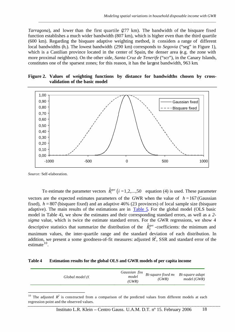
bandwidths between both fixed Gaussian and bisquare functions (167 and 807 km, respectively). Too large a bandwidth will produce a flat surface with little spatial variation and too small a bandwidth will result in estimation problems with some of the local regressions. On the contrary, the bisquare adaptive function establishes different local bandwidths (such that each sub-sample always includes the 46% of the Spanish provinces, which is about 23 of 50), in a range from 290 to 963 km, depending on the density of neighbors around each province. Figure 2 shows the spatial range of the two fixed weighting schemes used in this application, Gaussian and bisquare, computed for their corresponding cross-validated bandwidths (167 and 807 km, respectively). In current GWR techniques, bandwidth is first established globally, with fixed weighting schemes (Gaussian or bisquare), meaning that regions in denser parts of the study area have a larger number of weighted neighbors contributing to their estimates than in less dense parts. The bandwidth of the Gaussian fixed weighting function (167 km) is about half the greatest nearest neighbor distance in the data set (264 km, for the Balearic Islands and
9 To give a point location value to each observation, we used the centroid of each province.
Modeling spatial variations in household disposable income with GWR __________________________________________________________________________________________
Instituto L.R. Klein – Centro Gauss. U.A.M. D.T. nº 15. February 2006
18
Tarragona), and lower than the first quartile (277 km). The bandwidth of the bisquare fixed function establishes a much wider bandwidth (807 km), which is higher even than the third quartile (600 km). Regarding the bisquare adaptive weighting method, it considers a range of different local bandwidths (hi). The lowest bandwidth (290 km) corresponds to Segovia (“seg” in Figure 1), which is a Castilian province located in the center of Spain, the denser area (e.g. the zone with more proximal neighbors). On the other side, Santa Cruz de Tenerife (“scr”), in the Canary Islands, constitutes one of the sparsest zones; for this reason, it has the largest bandwidth, 963 km.
Figure 2. Values of weighting functions by distance for bandwidths chosen by cross-validation of the basic model
0,00
0,10
0,20
0,30
0,40
0,50
0,60
0,70
0,80
0,90
1,00
-1000 -500 0 500 1000
Gaussian fixed
Bisquare fixed
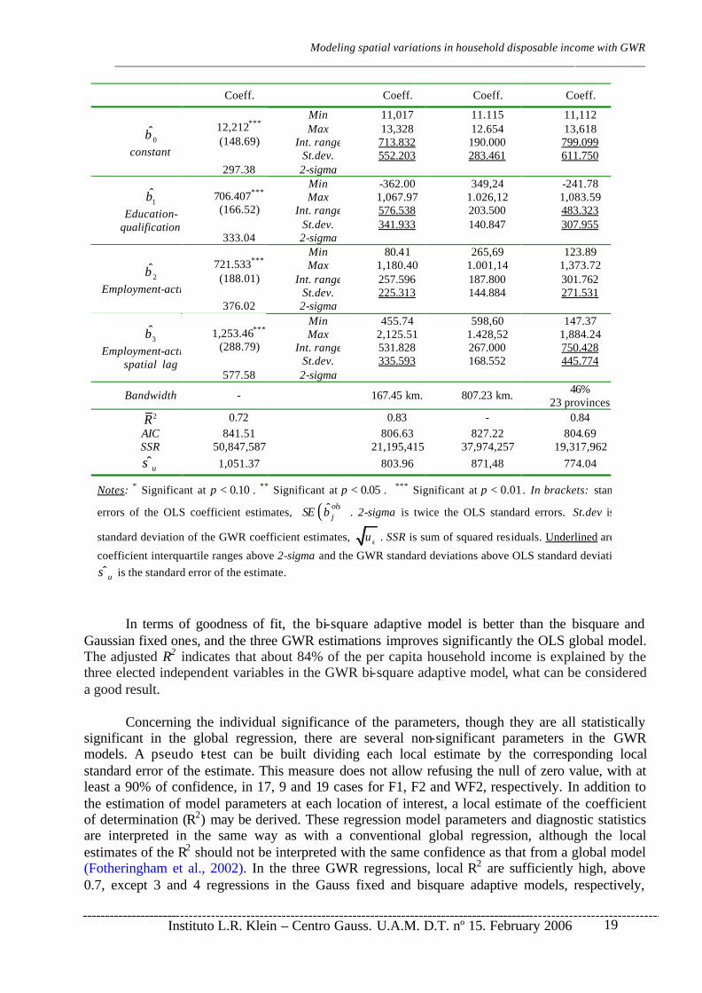
Source: Self-elaboration. To estimate the parameter vectors ( )gwrˆ 1,2,...,50iß i = equation (4) is used. These parameter vectors are the expected estimates parameters of the GWR when the value of 167h = (Gaussian fixed), 807h = (bisquare fixed) and an adaptive 46% (23 provinces) of local sample size (bisquare adaptive). The main results of the estimations are in Table 5. For the global model (OLS basic model in Table 4), we show the estimates and their corresponding standard errors, as well as a 2-sigma value, which is twice the estimate standard errors. For the GWR regressions, we show 4 descriptive statistics that summarize the distribution of the gwrˆ
ijß -coefficients: the minimum and maximum values, the inter-quartile range and the standard deviation of each distribution. In addition, we present a some goodness-of- fit measures: adjusted R2, SSR and standard error of the estimate10. Table 4 Estimation results for the global OLS and GWR models of per capita income
Global model (OLS) Gaussian fixed
model (GWR)
Bi-square fixed model(GWR)
Bi-square adaptive model (GWR)
10 The adjusted R2 is constructed from a comparison of the predicted values from different models at each regression point and the observed values.
Modeling spatial variations in household disposable income with GWR __________________________________________________________________________________________
Instituto L.R. Klein – Centro Gauss. U.A.M. D.T. nº 15. February 2006
19
Coeff. Coeff. Coeff. Coeff.
Min 11,017 11.115 11,112 Max 13,328 12.654 13,618
Int. range 713.832 190.000 799.099 12,212*** (148.69)
St.dev. 552.203 283.461 611.750 0β̂
constant
297.38 2-sigma Min -362.00 349,24 -241.78 Max 1,067.97 1.026,12 1,083.59
Int. range 576.538 203.500 483.323 706.407*** (166.52)
St.dev. 341.933 140.847 307.955
1̂β Education-
qualification333.04 2-sigma
Min 80.41 265,69 123.89 Max 1,180.40 1.001,14 1,373.72
Int. range 257.596 187.800 301.762 721.533*** (188.01)
St.dev. 225.313 144.884 271.531 2β̂
Employment-activity376.02 2-sigma
Min 455.74 598,60 147.37 Max 2,125.51 1.428,52 1,884.24
Int. range 531.828 267.000 750.428 1,253.46***
(288.79) St.dev. 335.593 168.552 445.774
3̂β Employment-activity
spatial lag 577.58 2-sigma
Bandwidth - 167.45 km. 807.23 km. 46% 23 provinces
2R 0.72 0.83 - 0.84 AIC 841.51 806.63 827.22 804.69 SSR 50,847,587 21,195,415 37,974,257 19,317,962 ˆuσ 1,051.37 803.96 871,48 774.04
Notes: * Significant at 0.10p < . ** Significant at 0.05p < . *** Significant at 0.01p < . In brackets: standard
errors of the OLS coefficient estimates, ( )ˆ olsjSE β . 2-sigma is twice the OLS standard errors. St.dev is the
standard deviation of the GWR coefficient estimates, kυ . SSR is sum of squared residuals. Underlined are the
coefficient interquartile ranges above 2-sigma and the GWR standard deviations above OLS standard deviations. ˆuσ is the standard error of the estimate.
In terms of goodness of fit, the bi-square adaptive model is better than the bisquare and Gaussian fixed ones, and the three GWR estimations improves significantly the OLS global model. The adjusted R2 indicates that about 84% of the per capita household income is explained by the three elected independent variables in the GWR bi-square adaptive model, what can be considered a good result. Concerning the individual significance of the parameters, though they are all statistically significant in the global regression, there are several non-significant parameters in the GWR models. A pseudo t-test can be built dividing each local estimate by the corresponding local standard error of the estimate. This measure does not allow refusing the null of zero value, with at least a 90% of confidence, in 17, 9 and 19 cases for F1, F2 and WF2, respectively. In addition to the estimation of model parameters at each location of interest, a local estimate of the coefficient of determination (R2) may be derived. These regression model parameters and diagnostic statistics are interpreted in the same way as with a conventional global regression, although the local estimates of the R2 should not be interpreted with the same confidence as that from a global model (Fotheringham et al., 2002). In the three GWR regressions, local R2 are sufficiently high, above 0.7, except 3 and 4 regressions in the Gauss fixed and bisquare adaptive models, respectively,
Modeling spatial variations in household disposable income with GWR __________________________________________________________________________________________
Instituto L.R. Klein – Centro Gauss. U.A.M. D.T. nº 15. February 2006
20
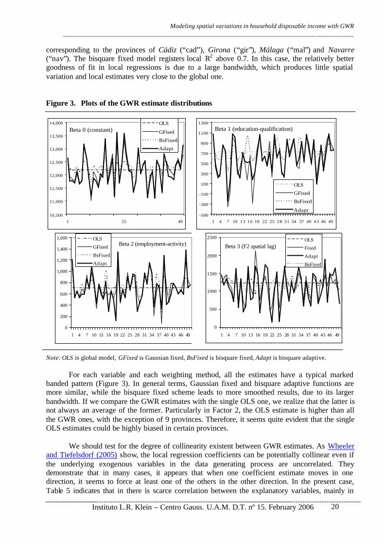
corresponding to the provinces of Cádiz (“cad”), Girona (“gir”), Málaga (“mal”) and Navarre (“nav”). The bisquare fixed model registers local R2 above 0.7. In this case, the relatively better goodness of fit in local regressions is due to a large bandwidth, which produces little spatial variation and local estimates very close to the global one. Figure 3. Plots of the GWR estimate distributions
Beta 0 (constant)
10,500
11,000
11,500
12,000
12,500
13,000
13,500
14,000
1 25 49
OLS
GFixed
BsFixed
Adapt
Beta 1 (education-qualification)
-500
-300
-100
100
300
500
700
900
1100
1300
1 4 7 10 13 16 19 22 25 28 31 34 37 40 43 46 49
OLS
GFixed
BsFixed
Adapt
Beta 2 (employment-activity)
0
200
400
600
800
1,000
1,200
1,400
1,600
1 4 7 10 13 16 19 22 25 28 31 34 37 40 43 46 49
OLS
GFixed
BsFixed
Adapt
Beta 3 (F2 spatial lag)
0
500
1000
1500
2000
2500
1 4 7 10 13 16 19 22 25 28 31 34 37 40 43 46 49
OLS
Fixed
Adapt
BsFixed
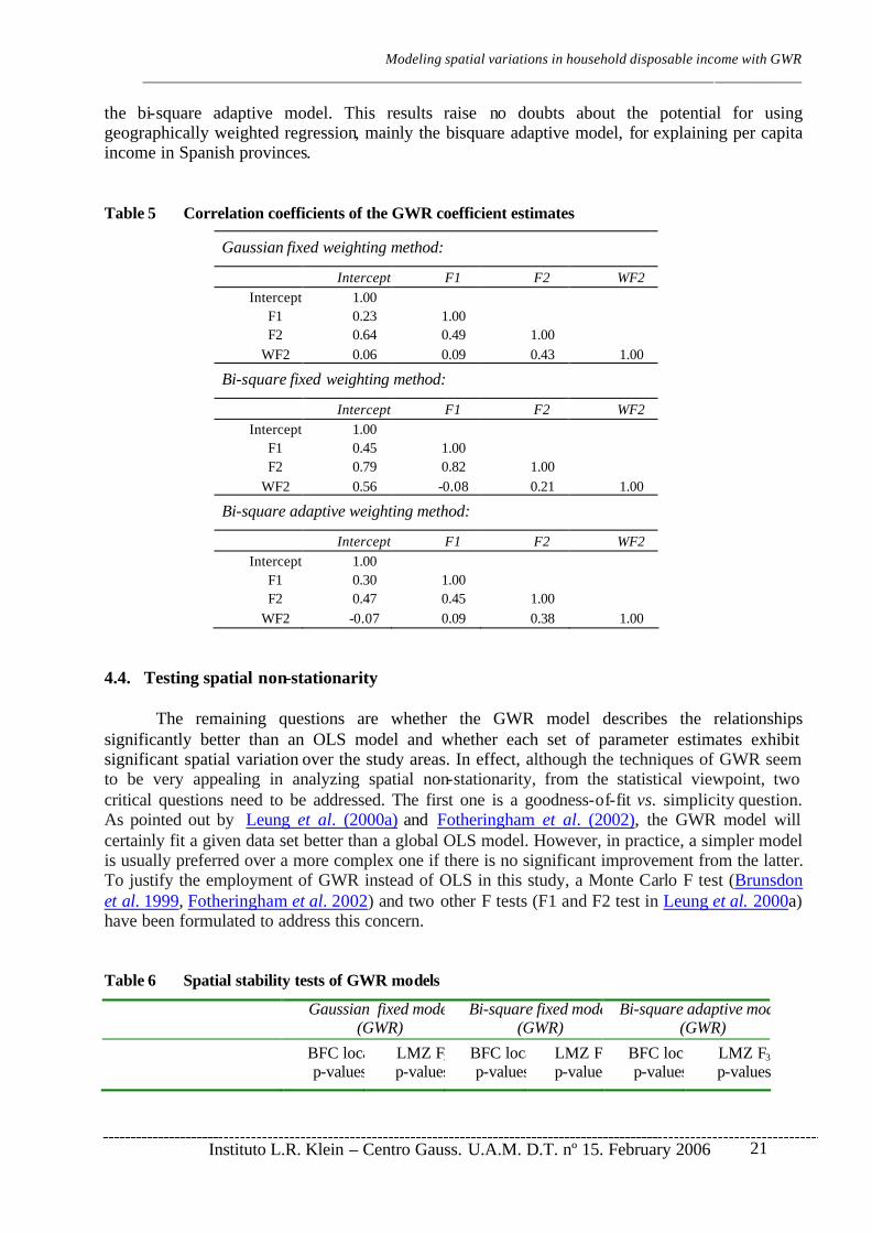
Note: OLS is global model, GFixed is Gaussian fixed, BsFixed is bisquare fixed, Adapt is bisquare adaptive. For each variable and each weighting method, all the estimates have a typical marked banded pattern (Figure 3). In general terms, Gaussian fixed and bisquare adaptive functions are more similar, while the bisquare fixed scheme leads to more smoothed results, due to its larger bandwidth. If we compare the GWR estimates with the single OLS one, we realize that the latter is not always an average of the former. Particularly in Factor 2, the OLS estimate is higher than all the GWR ones, with the exception of 9 provinces. Therefore, it seems quite evident that the single OLS estimates could be highly biased in certain provinces. We should test for the degree of collinearity existent between GWR estimates. As Wheeler and Tiefelsdorf (2005) show, the local regression coefficients can be potentially collinear even if the underlying exogenous variables in the data generating process are uncorrelated. They demonstrate that in many cases, it appears that when one coefficient estimate moves in one direction, it seems to force at least one of the others in the other direction. In the present case, Table 5 indicates that in there is scarce correlation between the explanatory variables, mainly in
Modeling spatial variations in household disposable income with GWR __________________________________________________________________________________________
Instituto L.R. Klein – Centro Gauss. U.A.M. D.T. nº 15. February 2006
21
the bi-square adaptive model. This results raise no doubts about the potential for using geographically weighted regression, mainly the bisquare adaptive model, for explaining per capita income in Spanish provinces. Table 5 Correlation coefficients of the GWR coefficient estimates
Gaussian fixed weighting method:
Intercept F1 F2 WF2 Intercept 1.00
F1 0.23 1.00 F2 0.64 0.49 1.00
WF2 0.06 0.09 0.43 1.00
Bi-square fixed weighting method:
Intercept F1 F2 WF2 Intercept 1.00
F1 0.45 1.00 F2 0.79 0.82 1.00
WF2 0.56 -0.08 0.21 1.00
Bi-square adaptive weighting method:
Intercept F1 F2 WF2 Intercept 1.00
F1 0.30 1.00 F2 0.47 0.45 1.00
WF2 -0.07 0.09 0.38 1.00 4.4. Testing spatial non-stationarity The remaining questions are whether the GWR model describes the relationships significantly better than an OLS model and whether each set of parameter estimates exhibit significant spatial variation over the study areas. In effect, although the techniques of GWR seem to be very appealing in analyzing spatial non-stationarity, from the statistical viewpoint, two critical questions need to be addressed. The first one is a goodness-of-fit vs. simplicity question. As pointed out by Leung et al. (2000a) and Fotheringham et al. (2002), the GWR model will certainly fit a given data set better than a global OLS model. However, in practice, a simpler model is usually preferred over a more complex one if there is no significant improvement from the latter. To justify the employment of GWR instead of OLS in this study, a Monte Carlo F test (Brunsdon et al. 1999, Fotheringham et al. 2002) and two other F tests (F1 and F2 test in Leung et al. 2000a) have been formulated to address this concern. Table 6 Spatial stability tests of GWR models
Gaussian fixed model (GWR)
Bi-square fixed model (GWR)
Bi-square adaptive model (GWR)
BFC localp-values
LMZ F3
p-valuesBFC localp-values
LMZ F3
p-valuesBFC localp-values
LMZ F3
p-values

Modeling spatial variations in household disposable income with GWR __________________________________________________________________________________________
Instituto L.R. Klein – Centro Gauss. U.A.M. D.T. nº 15. February 2006
22
0β̂ constant
0.030** 0.605 - 0.232 0.00** 0.520
1̂β Education-qualification
0.320 0.088* - 0.230 0.43 0.000***
2β̂ Employment-activity
0.760 1.000 - 1.000 0.70 1.000
3̂β F1 spatial lag
0.890 1.000 - 1.000 0.72 1.000
BFC 0.017** 0.039** 0.008***
LMZ F1 0.123 0.313 0.092* Global
variability pvalues
LMZ F2 0.119 0.073* 0.092*
Moran’s I 0.011 0.162** -0.059
Notes: * Significant at 0.10p < . ** Significant at 0.05p < . *** Significant at 0.01p < .
These F-tests are based on analysis of variance (ANOVA) and use generalized degrees of freedom (no longer integer because of the varying weights sums per estimate) to compare the improved sum of squares accounted for by the GWR estimates as compared with the global OLS estimates. These tests are established so that a hat matrix may be constructed from rows from the GWR model, each row using its appropriate weights. The Monte Carlo test derived by Brunsdon et al. (1999) compares the difference in the residual sums of squares of the OLS and GWR models with the residual sum of squares of the GWR model. We will call it “global BFC test”. On their side, Leung et al. (2000a) proposed two other Monte Carlo tests, which are very similar to the global BFC: LMZ F1 and F2. The LMZ F1 compares the residual sums of squares of the GWR model with the residual sums of squares of the OLS one, with the corresponding degrees of freedom. On its side, the LMZ F2 is very similar to global BFC: it compares the same difference than in global BFC with the residual sum of squares of the OLS model, choosing a different denominator for the F-ratio, as well as slightly different degrees of freedom. Results of these tests are shown in Table 6, from which we can see that the GWR estimates significantly reduce the residual sum of squares over and above the OLS estimates, specially in the case of the bisquare specifications. The global BFC tests are significant in the three GWR models, though the F1 and F2 are not significant in the Gaussian fixed model. The second question concerns the core concept of employing a GWR model, namely, whether there is significant spatial non-stationarity among the relationships or not. To answer this question, another F test (the F3 test in Leung et al. 2000a), based on the sample variance of the estimated model coefficients have been suggested as well. If any independent variable (including the constant term) shows spatial stationarity by this test, a mixed GWR model may be more appropriate than OLS. In Table 6, we display two local statistics to test spatial variation in each GWR individual coefficients: BFC local test and LMZ F3 test. The BFC local is a Monte Carlo test to see if the local parameter estimates are stationary or non-stationary. BFC local test shows that only the independent term varies significantly over space, while LMZ F3 highlights spatial variation in F1 (education-qualification) parameter.
Modeling spatial variations in household disposable income with GWR __________________________________________________________________________________________
Instituto L.R. Klein – Centro Gauss. U.A.M. D.T. nº 15. February 2006
23
Brunsdon et al. 1998a, 1999, Mei 2004 and Fotheringham et al. 2002 also suggest the use of intuitive alternative methods that can overcome some of the disadvantages of the significance tests. In this sense, they present two informal proceedings. First, they compare the variability of the
gwrijβ -coefficients with the standard errors of the ols
jβ -coefficients of the global regression model
(1). This can be done by tabulating ( )2k ik ki
Nυ β β ⋅= −∑ , for each variable, against ( )kSE b
from model (1). If the null hypothesis of stationarity were rejected for some but not all parameters, a mixed GWR-model could be appropriate. In Table 5, all the values of kυ exceeds ( )ˆ ols
jSE β ,
although by less amounts in the cases of the non-significant variables (F2 and WF2). This suggests that there is some justification in considering the patterns of spatial variation in all the coefficients in the model. Secondly, we can also compare the range of the local parameter estimates ( ˆ gwr
ijβ ) with a
confidence interval around the global estimate of the equivalent parameter ( ˆ olsjβ ). Recall that 50%
of the local parameter values will be between the upper and lower quartiles and that approximately 68% of values in a normal distribution will be within ± 1 standard deviations of the mean. This gives us a reasonable, although very informal, means of comparison. We can compare the range of values of the local estimates ( ˆ gwr
ijβ ) between the lower and upper quartiles with the range of values
at ±1 standard deviations of the respective global estimate, which is simply ( )ˆ2 olsjSE β× . Given
that 68% of the values would be expected to lie within this latter interval, compared to 50% in the inter-quartile range, if the range of local estimates between the inter-quartile range is greater than that of 2 standard errors of the global mean, this suggests the relationship might be non-stationary. As we can see in Table 5, in the bi-square adaptive regression, only the interquartile range of the F2 (employment-activity) estimates is less than 2 standard errors (2-sigma) of its corresponding global estimate. These results reinforce the conclusion about the existence of spatial variation in the intercept and F1 (education-qualification) variable, though some spatial instability has also been found in WF2 (employment-activity in neighboring provinces). To give a further indication of the nature of the variation in the coefficients, we can consider the range of coefficient values estimated for the explanatory variables of income per capita with the help of a density plot11 (Bivand and Brunstad 2002). Figure 4 shows for each coefficient the density plot of the GWR coefficient distributions, as well as the OLS global estimate (solid vertical line) with its corresponding confidence bands (+/- twice the standard error) in dashed vertical lines. In all the cases, the GWR estimates group more or less around the OLS global estimates. These plots highlight the skewed shape of the bisquared fixed GWR distributions, due to the wider bandwidth (807 km) reached by this method with respect to the others. As stated before, too large a bandwidth will produce a flat surface with little spatial variation, and vice versa. Figure 4. Density plots of the GWR estimates
11 The density plot draws the non-parametric kernel density estimates of the coefficient distributions. It may be interpreted as the continuous equivalent of a histogram in which the number of intervals has been set to infinity and then to the continuum.

Modeling spatial variations in household disposable income with GWR __________________________________________________________________________________________
Instituto L.R. Klein – Centro Gauss. U.A.M. D.T. nº 15. February 2006
24
1 1.1 1.2 1.3 1.4 1.5
x 104
0
0.2
0.4
0.6
0.8
1
1.2
1.4
1.6
1.8
2x 10
-3 Intercept
gauss fixedbisquare fixedbisquare adaptive
-1000 -500 0 500 1000 1500 20000
0.5
1
1.5
2
2.5x 10
-3 F1 (education-qualification)
gaussian fixedbisquared fixedbisquared adaptive
-500 0 500 1000 1500 20000
0.5
1
1.5
2
2.5
3x 10
-3 F2 (employment-activity)gauss fixedbisquare fixedbisquare adaptive
-500 0 500 1000 1500 2000 2500 30000
0.5
1
1.5
2
2.5
3x 10
-3 WF2 (employment-activity spatial lag)gauss fixedbisquared fixedbisquared adaptive
Notes: Vertical solid lines are the OLS estimators of the global basic model; vertical dashed lines are their corresponding 2-sigma values (+/- twice the estimator standard errors). It also seems clear that there is a certain degree of structural instability in GWR coefficients with respect to OLS, since some of the former are out the latter 2-sigma bands, especially in the bisquare adaptive distributions. In the case of the intercept and F1 (education-qualification), spatial variability is more acute because there are more GWR coefficients significantly exceeding the OLS bands. On the contrary, spatial instability is lower in F2 (employment-activity) and WF2 (employment-activity spatial lag) because they have a higher density mass inside the OLS 2-sigma bands. This result confirms the output of the local instability tests: though the informal measures are more or less significant for all the coefficients, in the GWR bisquare adaptive model (Table 4) the formal tests (Table 5) are only clearly significant for the intercept (BFC local) and the variable F1 of education-qualification (LMZ F3). Finally, we can test for spatial autocorrelation in the residuals with the help of the Moran’s I test12 (Cliff and Ord 1981), which also allows us to detect remaining spatial non-stationarity (Fingleton 1999). Except for the bisquare fixed function, GWR models lead to uncorrelated and stationary residuals what proves the superiority of GWR over the OLS global model.
12 The Moran’s I test has been computed on errors using the expression commonly applied to univariate distributions and the same spatial weight matrix used previously in the LM tests. Inference is based on the permutation approach (999 permutations), as shown in (Anselin 1995). There is also a test procedure for spatial autocorrelation in GWR framework in Leung et al. (2000b), which is a three-moment χ2 approximation.
Modeling spatial variations in household disposable income with GWR __________________________________________________________________________________________
Instituto L.R. Klein – Centro Gauss. U.A.M. D.T. nº 15. February 2006
25
In short, since results demonstrate the existence of spatial instability in the parameters, we can conclude that GWR regression is better than a global model to explain income in Spanish provinces. We have tested this hypothesis using three different weighting functions and all them address to this same conclusion. We choose the bisquare adaptive function since it leads to a better goodness of fit and can adapt to the different spatial configurations of Spanish provinces across territory (e.g. it considers different bandwidths for each province depending on its spatial sparseness). Moreover, this function also overcomes better the multicollinearity problems between the estimates and produces white noise residuals. Regarding local non-stationarity of the bisquare adaptive GWR estimates, the formal tests are only clearly significant for the intercept and F1 (education-qualification), though the informal local tests are also significant (in a lesser extent) for the other two variables. Next, we analyze in depth the distribution of these estimates across the Spanish territory. 4.5. Analysis of spatial instability in bisquare adaptive GWR estimators First, we map the spatial variation of these two variables, intercept and F1, to have a better knowledge of variation on their fitted parameters (Figure 5). Indeed, especially when working with large data sets, mapping, or some other form of visualization, is the only way to make sense of nature of spatial instability. In our model, the intercept or constant parameter measures the fundamental level of per capita household income excluding the effects of all factors on regional economic development across Spain. It can be referred to as “the basic level of regional economic development”. There is a clear spatial variation with higher constant parameters in the northeastern provinces and lower ones in the southern provinces. It means that, other things being equal, the northeastern Spanish provinces had the highest basic level of economic development; the southern provinces had the lowest, while the level in the central -and northwestern- areas are between the northeastern and the southern areas in 2004. Thus, the basic level of economic development in the Spanish provinces displays a ladder-step distribution, which varies from high in the northeast to low in the south. In Figure 5, we have also represented Factor 1 (education-qualification) coefficients. This variable has more impact on per capita household income in the north (Cantabria, the Bask Country, north Castile, Navarre, La Rioja) and west (Salamanca and Cáceres). On the other side, the influence of this factor on per capita income is less important in the Mediterranean provinces (Catalonia, The Balearics, Comunidad Valenciana, Murcia, south Andalusia and the Canaries), having this variable a negative effect in the Balearics. This is likely because these areas are growing economies based on the service sector, which is mainly labor- intensive and not so dependent on the education level of the labor force. On the contrary, in the north, economic activity is based on heavy industries, which are not so highly labor demanding, though require qualified workers. Figure 5. Map for the intercept and F1 adaptive GWR estimates

Modeling spatial variations in household disposable income with GWR __________________________________________________________________________________________
Instituto L.R. Klein – Centro Gauss. U.A.M. D.T. nº 15. February 2006
26
girgirgirgirgirgirgirgirgirgirgirgirgirgirg irg irg irg irg irg irg irg irg irg irg irg irg irgirgirgirgirgirgirgirgirgirgirgirgirgirgirg irg irg irg irg irg irg irg ir
barbarbarbarbarbarbarbarbarbarbarbarbarbarbarbarbarbarbarbarbarbarbarbarbarbarbarbarbarbarbarbarbarbarbarbarbarbarbarbarbarbarbarbarbarbarbarbarbar
navnavnavnavnavnavnavnavnavnavnavnavnavnavnavnavnavnavnavnavnavnavnavnavnavnavnavnavnavnavnavnavnavnavnavnavnavnavnavnavnavnavnavnavnavnavnavnavnav
llellellellellellellel l el l el l el l el l el l el l el l el l el l el l el l el l el l ellellellellellellellellellellellellellellellellellellellellel l el l el l el l el l el l el l ellehuehuehuehuehuehuehuehuehuehuehuehuehuehuehuehuehuehuehuehuehuehuehuehuehuehuehuehuehuehuehuehuehuehuehuehuehuehuehuehuehuehuehuehuehuehuehuehuehue
tartartartartartartartartartartartartartartartartartartartartartartartartartartartartartartartartartartartartartartartartartartartartartartartartar
zarzarzarzarzarzarzarzarzarzarzarzarzarzarzarzarzarzarzarzarzarzarzarzarzarzarzarzarzarzarzarzarzarzarzarzarzarzarzarzarzarzarzarzarzarzarzarzarzar
guiguiguiguiguiguiguiguiguiguiguiguiguiguiguiguiguiguiguiguiguiguiguiguiguiguiguiguiguiguiguiguiguiguiguiguiguiguiguiguiguiguiguiguiguiguiguiguigui
alaalaalaalaalaalaalaalaalaalaalaalaalaalaalaalaalaalaalaalaalaalaalaalaalaalaalaalaalaalaalaalaalaalaalaalaalaalaalaalaalaalaalaalaalaalaalaalaala
riorioriorioriorioriorioriorioriorioriorioriorioriorioriorioriorioriorioriorioriorioriorioriorioriorioriorioriorioriorioriorioriorioriorioriorioriosorsorsorsorsorsorsorsorsorsorsorsorsorsorsorsorsorsorsorsorsorsorsorsorsorsorsorsorsorsorsorsorsorsorsorsorsorsorsorsorsorsorsorsorsorsorsorsorsor
burburburburburburburburburburburburburburburburburburburburburburburburburburburburburburburburburburburburburburburburburburburburburburburburbur
segsegsegsegsegsegsegsegsegsegsegsegsegsegsegsegsegsegsegsegsegsegsegsegsegsegsegsegsegsegsegsegsegsegsegsegsegsegsegsegsegsegsegsegsegsegsegsegseg
palpalpalpalpalpalpalpalpalpalpalpalpalpalpalpalpalpalpalpalpalpalpalpalpalpalpalpalpalpalpalpalpalpalpalpalpalpalpalpalpalpalpalpalpalpalpalpalpal
vallvallvallvallvallvallvallvallvallvallvallvallvallvallvallvallvallvallvallvallvallvallvallvallvallvallvallvallvallvallvallvallvallvallvallvallvallvallvallvallvallvallvallvallvallvallvallvallvall
vizvizvizvizvizvizvizvizvizvizvizvizvizvizvizvizvizvizvizvizvizvizvizvizvizvizvizvizvizvizvizvizvizvizvizvizvizvizvizvizvizvizvizvizvizvizvizvizvizcancancancancancancancancancancancancancancancancancancancancancancancancancancancancancancancancancancancancancancancancancancancancancancancancanastastastastastastastastastastastastastastastastastastastastastastastastastastastastastastastastastastastastastastastastastastastastastastastastast
cadcadcadcadcadcadcadcadcadcadcadcadcadcadcadcadcadcadcadcadcadcadcadcadcadcadcadcadcadcadcadcadcadcadcadcadcadcadcadcadcadcadcadcadcadcadcadcadcadmalmalmalmalmalmalmalmalmalmalmalmalmalmalmalmalmalmalmalmalmalmalmalmalmalmalmalmalmalmalmalmalmalmalmalmalmalmalmalmalmalmalmalmalmalmalmalmalmal
s e vs e vs e vs e vs e vs e vs e vsevsevsevsevsevsevsevsevsevsevsevsevsevsevsevsevsevsevsevsevs e vs e vs e vs e vs e vs e vs e vsevsevsevsevsevsevsevsevsevsevsevsevsevsevsev almalmalmalmalmalmalmalmalmalmalmalmalmalmalmalmalmalmalmalmalmalmalmalmalmalmalmalmalmalmalmalmalmalmalmalmalmalmalmalmalmalmalmalmalmalmalmalmalm
albalbalbalbalbalbalbalbalbalbalbalbalbalbalbalbalbalbalbalbalbalbalbalbalbalbalbalbalbalbalbalbalbalbalbalbalbalbalbalbalbalbalbalbalbalbalbalbalbjaejaejaejaejaejaejaejaejaejaejaejaejaejaejaejaejaejaejaejaejaejaejaejaejaejaejaejaejaejaejaejaejaejaejaejaejaejaejaejaejaejaejaejaejaejaejaejaejae
murmurmurmurmurmurmurmurmurmurmurmurmurmurmurmurmurmurmurmurmurmurmurmurmurmurmurmurmurmurmurmurmurmurmurmurmurmurmurmurmurmurmurmurmurmurmurmurmur
alial ial ial ial ial ial ialialialialialialialialialialialialialialial ial ial ial ial ial ial ial ial ial ial ial ial ialialialialialialialialialialialialialialial i
ponponponponponponponponponponponponponponponponponponponponponponponponponponponponponponponponponponponponponponponponponponponponponponponponpon
acoacoacoacoacoacoacoacoacoacoacoacoacoacoacoacoacoacoacoacoacoacoacoacoacoacoacoacoacoacoacoacoacoacoacoacoacoacoacoacoacoacoacoacoacoacoacoacoaco
palpalpalpalpalpalpalpalpalpalpalpalpalpalpalpalpalpalpalpalpalpalpalpalpalpalpalpalpalpalpalpalpalpalpalpalpalpalpalpalpalpalpalpalpalpalpalpalpal
valvalvalvalvalvalvalvalvalvalvalvalvalvalvalvalvalvalvalvalvalvalvalvalvalvalvalvalvalvalvalvalvalvalvalvalvalvalvalvalvalvalvalvalvalvalvalvalval
cascascascascascascascascascascascascascascascascascascascascascascascascascascascascascascascascascascascascascascascascascascascascascascascascas
balbalbalbalbalbalbalbalbalbalbalbalbalbalbalbalbalbalbalbalbalbalbalbalbalbalbalbalbalbalbalbalbalbalbalbalbalbalbalbalbalbalbalbalbalbalbalbalbal
scrscrscrscrscrscrscrscrscrscrscrscrscrscrscrscrscrscrscrscrscrscrscrscrscrscrscrscrscrscrscrscrscrscrscrscrscrscrscrscrscrscrscrscrscrscrscrscrscr
aviaviaviaviaviaviaviaviaviaviaviaviaviaviaviaviaviaviaviaviaviaviaviaviaviaviaviaviaviaviaviaviaviaviaviaviaviaviaviaviaviaviaviaviaviaviaviaviavi
badbadbadbadbadbadbadbadbadbadbadbadbadbadbadbadbadbadbadbadbadbadbadbadbadbadbadbadbadbadbadbadbadbadbadbadbadbadbadbadbadbadbadbadbadbadbadbadbad
caccaccaccaccaccaccaccaccaccaccaccaccaccaccaccaccaccaccaccaccaccaccaccaccaccaccaccaccaccaccaccaccaccaccaccaccaccaccaccaccaccaccaccaccaccaccaccaccac
crecrecrecrecrecrecrecrecrecrecrecrecrecrecrecrecrecrecrecrecrecrecrecrecrecrecrecrecrecrecrecrecrecrecrecrecrecrecrecrecrecrecrecrecrecrecrecrecre
corcorcorcorcorcorcorcorcorcorcorcorcorcorcorcorcorcorcorcorcorcorcorcorcorcorcorcorcorcorcorcorcorcorcorcorcorcorcorcorcorcorcorcorcorcorcorcorcor
cuecuecuecuecuecuecuecuecuecuecuecuecuecuecuecuecuecuecuecuecuecuecuecuecuecuecuecuecuecuecuecuecuecuecuecuecuecuecuecuecuecuecuecuecuecuecuecuecue
gragragragragragragragragragragragragragragragragragragragragragragragragragragragragragragragragragragragragragragragragragragragragragragragragra
guaguaguaguaguaguaguaguaguaguaguaguaguaguaguaguaguaguaguaguaguaguaguaguaguaguaguaguaguaguaguaguaguaguaguaguaguaguaguaguaguaguaguaguaguaguaguaguagua
huehuehuehuehuehuehuehuehuehuehuehuehuehuehuehuehuehuehuehuehuehuehuehuehuehuehuehuehuehuehuehuehuehuehuehuehuehuehuehuehuehuehuehuehuehuehuehuehue
leoleoleoleoleoleoleoleoleoleoleoleoleoleoleoleoleoleoleoleoleoleoleoleoleoleoleoleoleoleoleoleoleoleoleoleoleoleoleoleoleoleoleoleoleoleoleoleoleolugluglugluglugluglugluglugluglugluglugluglugluglugluglugluglugluglugluglugluglugluglugluglugluglugluglugluglugluglugluglugluglugluglugluglugluglug
madmadmadmadmadmadmadmadmadmadmadmadmadmadmadmadmadmadmadmadmadmadmadmadmadmadmadmadmadmadmadmadmadmadmadmadmadmadmadmadmadmadmadmadmadmadmadmadmad
ourourourourourourourourourourourourourourourourourourourourourourourourourourourourourourourourourourourourourourourourourourourourourourourourour
salsalsalsalsalsalsalsalsalsalsalsalsalsalsalsalsalsalsalsalsalsalsalsalsalsalsalsalsalsalsalsalsalsalsalsalsalsalsalsalsalsalsalsalsalsalsalsalsal terterterterterterterterterterterterterterterterterterterterterterterterterterterterterterterterterterterterterterterterterterterterterterterterter
toltoltoltoltoltoltoltoltoltoltoltoltoltoltoltoltoltoltoltoltoltoltoltoltoltoltoltoltoltoltoltoltoltoltoltoltoltoltoltoltoltoltoltoltoltoltoltoltol
zamzamzamzamzamzamzamzamzamzamzamzamzamzamzamzamzamzamzamzamzamzamzamzamzamzamzamzamzamzamzamzamzamzamzamzamzamzamzamzamzamzamzamzamzamzamzamzamzam
Intercept
11,110 to 11,86011,860 to 12,53012,530 to 13,620
girgirgirgirgirgirgirgirgirgirgirgirgirgirg irg irg irg irg irg irg irg irg irg irg irg irg irgirgirgirgirgirgirgirgirgirgirgirgirgirgirg irg irg irg irg irg irg irg ir
barbarbarbarbarbarbarbarbarbarbarbarbarbarbarbarbarbarbarbarbarbarbarbarbarbarbarbarbarbarbarbarbarbarbarbarbarbarbarbarbarbarbarbarbarbarbarbarbar
navnavnavnavnavnavnavnavnavnavnavnavnavnavnavnavnavnavnavnavnavnavnavnavnavnavnavnavnavnavnavnavnavnavnavnavnavnavnavnavnavnavnavnavnavnavnavnavnav
llellellellellellellel l el l el l el l el l el l el l el l el l el l el l el l el l el l ellellellellellellellellellellellellellellellellellellellellel l el l el l el l el l el l el l ellehuehuehuehuehuehuehuehuehuehuehuehuehuehuehuehuehuehuehuehuehuehuehuehuehuehuehuehuehuehuehuehuehuehuehuehuehuehuehuehuehuehuehuehuehuehuehuehuehue
tartartartartartartartartartartartartartartartartartartartartartartartartartartartartartartartartartartartartartartartartartartartartartartartartar
zarzarzarzarzarzarzarzarzarzarzarzarzarzarzarzarzarzarzarzarzarzarzarzarzarzarzarzarzarzarzarzarzarzarzarzarzarzarzarzarzarzarzarzarzarzarzarzarzar
guiguiguiguiguiguiguiguiguiguiguiguiguiguiguiguiguiguiguiguiguiguiguiguiguiguiguiguiguiguiguiguiguiguiguiguiguiguiguiguiguiguiguiguiguiguiguiguigui
alaalaalaalaalaalaalaalaalaalaalaalaalaalaalaalaalaalaalaalaalaalaalaalaalaalaalaalaalaalaalaalaalaalaalaalaalaalaalaalaalaalaalaalaalaalaalaalaala
riorioriorioriorioriorioriorioriorioriorioriorioriorioriorioriorioriorioriorioriorioriorioriorioriorioriorioriorioriorioriorioriorioriorioriorioriosorsorsorsorsorsorsorsorsorsorsorsorsorsorsorsorsorsorsorsorsorsorsorsorsorsorsorsorsorsorsorsorsorsorsorsorsorsorsorsorsorsorsorsorsorsorsorsorsor
burburburburburburburburburburburburburburburburburburburburburburburburburburburburburburburburburburburburburburburburburburburburburburburburbur
segsegsegsegsegsegsegsegsegsegsegsegsegsegsegsegsegsegsegsegsegsegsegsegsegsegsegsegsegsegsegsegsegsegsegsegsegsegsegsegsegsegsegsegsegsegsegsegseg
palpalpalpalpalpalpalpalpalpalpalpalpalpalpalpalpalpalpalpalpalpalpalpalpalpalpalpalpalpalpalpalpalpalpalpalpalpalpalpalpalpalpalpalpalpalpalpalpal
vallvallvallvallvallvallvallvallvallvallvallvallvallvallvallvallvallvallvallvallvallvallvallvallvallvallvallvallvallvallvallvallvallvallvallvallvallvallvallvallvallvallvallvallvallvallvallvallvall
vizvizvizvizvizvizvizvizvizvizvizvizvizvizvizvizvizvizvizvizvizvizvizvizvizvizvizvizvizvizvizvizvizvizvizvizvizvizvizvizvizvizvizvizvizvizvizvizvizcancancancancancancancancancancancancancancancancancancancancancancancancancancancancancancancancancancancancancancancancancancancancancancancancanastastastastastastastastastastastastastastastastastastastastastastastastastastastastastastastastastastastastastastastastastastastastastastastastast
cadcadcadcadcadcadcadcadcadcadcadcadcadcadcadcadcadcadcadcadcadcadcadcadcadcadcadcadcadcadcadcadcadcadcadcadcadcadcadcadcadcadcadcadcadcadcadcadcadmalmalmalmalmalmalmalmalmalmalmalmalmalmalmalmalmalmalmalmalmalmalmalmalmalmalmalmalmalmalmalmalmalmalmalmalmalmalmalmalmalmalmalmalmalmalmalmalmal
s e vs e vs e vs e vs e vs e vs e vsevsevsevsevsevsevsevsevsevsevsevsevsevsevsevsevsevsevsevsevs e vs e vs e vs e vs e vs e vs e vsevsevsevsevsevsevsevsevsevsevsevsevsevsevsev almalmalmalmalmalmalmalmalmalmalmalmalmalmalmalmalmalmalmalmalmalmalmalmalmalmalmalmalmalmalmalmalmalmalmalmalmalmalmalmalmalmalmalmalmalmalmalmalm
albalbalbalbalbalbalbalbalbalbalbalbalbalbalbalbalbalbalbalbalbalbalbalbalbalbalbalbalbalbalbalbalbalbalbalbalbalbalbalbalbalbalbalbalbalbalbalbalbjaejaejaejaejaejaejaejaejaejaejaejaejaejaejaejaejaejaejaejaejaejaejaejaejaejaejaejaejaejaejaejaejaejaejaejaejaejaejaejaejaejaejaejaejaejaejaejaejae
murmurmurmurmurmurmurmurmurmurmurmurmurmurmurmurmurmurmurmurmurmurmurmurmurmurmurmurmurmurmurmurmurmurmurmurmurmurmurmurmurmurmurmurmurmurmurmurmur
alial ial ial ial ial ial ialialialialialialialialialialialialialialial ial ial ial ial ial ial ial ial ial ial ial ial ialialialialialialialialialialialialialialial i
ponponponponponponponponponponponponponponponponponponponponponponponponponponponponponponponponponponponponponponponponponponponponponponponponpon
acoacoacoacoacoacoacoacoacoacoacoacoacoacoacoacoacoacoacoacoacoacoacoacoacoacoacoacoacoacoacoacoacoacoacoacoacoacoacoacoacoacoacoacoacoacoacoacoaco
palpalpalpalpalpalpalpalpalpalpalpalpalpalpalpalpalpalpalpalpalpalpalpalpalpalpalpalpalpalpalpalpalpalpalpalpalpalpalpalpalpalpalpalpalpalpalpalpal
valvalvalvalvalvalvalvalvalvalvalvalvalvalvalvalvalvalvalvalvalvalvalvalvalvalvalvalvalvalvalvalvalvalvalvalvalvalvalvalvalvalvalvalvalvalvalvalval
cascascascascascascascascascascascascascascascascascascascascascascascascascascascascascascascascascascascascascascascascascascascascascascascascas
balbalbalbalbalbalbalbalbalbalbalbalbalbalbalbalbalbalbalbalbalbalbalbalbalbalbalbalbalbalbalbalbalbalbalbalbalbalbalbalbalbalbalbalbalbalbalbalbal
scrscrscrscrscrscrscrscrscrscrscrscrscrscrscrscrscrscrscrscrscrscrscrscrscrscrscrscrscrscrscrscrscrscrscrscrscrscrscrscrscrscrscrscrscrscrscrscrscr
aviaviaviaviaviaviaviaviaviaviaviaviaviaviaviaviaviaviaviaviaviaviaviaviaviaviaviaviaviaviaviaviaviaviaviaviaviaviaviaviaviaviaviaviaviaviaviaviavi
badbadbadbadbadbadbadbadbadbadbadbadbadbadbadbadbadbadbadbadbadbadbadbadbadbadbadbadbadbadbadbadbadbadbadbadbadbadbadbadbadbadbadbadbadbadbadbadbad
caccaccaccaccaccaccaccaccaccaccaccaccaccaccaccaccaccaccaccaccaccaccaccaccaccaccaccaccaccaccaccaccaccaccaccaccaccaccaccaccaccaccaccaccaccaccaccaccac
crecrecrecrecrecrecrecrecrecrecrecrecrecrecrecrecrecrecrecrecrecrecrecrecrecrecrecrecrecrecrecrecrecrecrecrecrecrecrecrecrecrecrecrecrecrecrecrecre
corcorcorcorcorcorcorcorcorcorcorcorcorcorcorcorcorcorcorcorcorcorcorcorcorcorcorcorcorcorcorcorcorcorcorcorcorcorcorcorcorcorcorcorcorcorcorcorcor
cuecuecuecuecuecuecuecuecuecuecuecuecuecuecuecuecuecuecuecuecuecuecuecuecuecuecuecuecuecuecuecuecuecuecuecuecuecuecuecuecuecuecuecuecuecuecuecuecue
gragragragragragragragragragragragragragragragragragragragragragragragragragragragragragragragragragragragragragragragragragragragragragragragragra
guaguaguaguaguaguaguaguaguaguaguaguaguaguaguaguaguaguaguaguaguaguaguaguaguaguaguaguaguaguaguaguaguaguaguaguaguaguaguaguaguaguaguaguaguaguaguaguagua
huehuehuehuehuehuehuehuehuehuehuehuehuehuehuehuehuehuehuehuehuehuehuehuehuehuehuehuehuehuehuehuehuehuehuehuehuehuehuehuehuehuehuehuehuehuehuehuehue
leoleoleoleoleoleoleoleoleoleoleoleoleoleoleoleoleoleoleoleoleoleoleoleoleoleoleoleoleoleoleoleoleoleoleoleoleoleoleoleoleoleoleoleoleoleoleoleoleolugluglugluglugluglugluglugluglugluglugluglugluglugluglugluglugluglugluglugluglugluglugluglugluglugluglugluglugluglugluglugluglugluglugluglugluglug
madmadmadmadmadmadmadmadmadmadmadmadmadmadmadmadmadmadmadmadmadmadmadmadmadmadmadmadmadmadmadmadmadmadmadmadmadmadmadmadmadmadmadmadmadmadmadmadmad
ourourourourourourourourourourourourourourourourourourourourourourourourourourourourourourourourourourourourourourourourourourourourourourourourour
salsalsalsalsalsalsalsalsalsalsalsalsalsalsalsalsalsalsalsalsalsalsalsalsalsalsalsalsalsalsalsalsalsalsalsalsalsalsalsalsalsalsalsalsalsalsalsalsal terterterterterterterterterterterterterterterterterterterterterterterterterterterterterterterterterterterterterterterterterterterterterterterterter
toltoltoltoltoltoltoltoltoltoltoltoltoltoltoltoltoltoltoltoltoltoltoltoltoltoltoltoltoltoltoltoltoltoltoltoltoltoltoltoltoltoltoltoltoltoltoltoltol
zamzamzamzamzamzamzamzamzamzamzamzamzamzamzamzamzamzamzamzamzamzamzamzamzamzamzamzamzamzamzamzamzamzamzamzamzamzamzamzamzamzamzamzamzamzamzamzamzam
F1
-250 to 500500 to 770770 to 1,090
Notes: The classification method is “natural breaks” (Jenks and Caspall 1971) Mapping the spatial distributions of the GWR raw estimates is interesting. However, as Fotheringham et al. 2001 point out, the values represented on these maps do not take into account the standard errors of the estimates. Consequently, it is often more illuminating to view maps of t-statistics by dividing each local estimate by the corresponding local standard error of the estimate. These t-maps are useful, not in a formal sense, but in a purely exploratory role, to highlight parts of the map where interesting relationships appear to be occurring. In Figure 5, we have shown the t-maps for the GWR local parameters of the explanatory variables (we exclude the intercept since it is always significant). In general, a t-map of a certain coefficient is very similar to the map of this same raw coefficient, but sometimes reveals interesting spatial variations that would be missed completely if we rely solely on the global analysis of raw parameters. For example, in Figure 5 we see that F1 (education-qualification) has low influence on per capita income in the Mediterranean provinces and the Isles. However, with the help of the t-map we can also detect other non-significant provinces, such as the ones located in the northwest (Galicia). Nevertheless, in general, in these places the most significant variable is F2 (employment-activity). That is to say, there is a tradeoff between these 2 factors when explaining per capita household income. This conclusion was also reached before, when computing these factors as orthogonal, demonstrating that in Spain, there are provinces in which higher levels of education coexists with lower employment rates, and vice versa. Figure 6. t-Maps for the adaptive GWR estimates of the explanatory variables

Modeling spatial variations in household disposable income with GWR __________________________________________________________________________________________
Instituto L.R. Klein – Centro Gauss. U.A.M. D.T. nº 15. February 2006
27
alaalaalaalaalaalaalaalaalaalaalaalaalaalaalaalaalaalaalaalaalaalaalaalaalaalaalaalaalaalaalaalaalaalaalaalaalaalaalaalaalaalaalaalaalaalaalaalaala
burburburburburburburburburburburburburburburburburburburburburburburburburburburburburburburburburburburburburburburburburburburburburburburburburpalpalpalpalpalpalpalpalpalpalpalpalpalpalpalpalpalpalpalpalpalpalpalpalpalpalpalpalpalpalpalpalpalpalpalpalpalpalpalpalpalpalpalpalpalpalpalpalpal
cancancancancancancancancancancancancancancancancancancancancancancancancancancancancancancancancancancancancancancancancancancancancancancancancan
rioriorioriorioriorioriorioriorioriorioriorioriorioriorioriorioriorioriorioriorioriorioriorioriorioriorioriorioriorioriorioriorioriorioriorioriorio
vizvizvizvizvizvizvizvizvizvizvizvizvizvizvizvizvizvizvizvizvizvizvizvizvizvizvizvizvizvizvizvizvizvizvizvizvizvizvizvizvizvizvizvizvizvizvizvizvizguiguiguiguiguiguiguiguiguiguiguiguiguiguiguiguiguiguiguiguiguiguiguiguiguiguiguiguiguiguiguiguiguiguiguiguiguiguiguiguiguiguiguiguiguiguiguiguigui
segsegsegsegsegsegsegsegsegsegsegsegsegsegsegsegsegsegsegsegsegsegsegsegsegsegsegsegsegsegsegsegsegsegsegsegsegsegsegsegsegsegsegsegsegsegsegsegseg
navnavnavnavnavnavnavnavnavnavnavnavnavnavnavnavnavnavnavnavnavnavnavnavnavnavnavnavnavnavnavnavnavnavnavnavnavnavnavnavnavnavnavnavnavnavnavnavnav
cadcadcadcadcadcadcadcadcadcadcadcadcadcadcadcadcadcadcadcadcadcadcadcadcadcadcadcadcadcadcadcadcadcadcadcadcadcadcadcadcadcadcadcadcadcadcadcadcad
sevsevsevsevsevsevsevsevsevsevsevsevsevsevsevsevsevsevsevsevsevsevsevsevsevsevsevsevsevsevsevsevsevsevsevsevsevsevsevsevsevsevsevsevsevsevsevsevsev
almalmalmalmalmalmalmalmalmalmalmalmalmalmalmalmalmalmalmalmalmalmalmalmalmalmalmalmalmalmalmalmalmalmalmalmalmalmalmalmalmalmalmalmalmalmalmalmalmmurmurmurmurmurmurmurmurmurmurmurmurmurmurmurmurmurmurmurmurmurmurmurmurmurmurmurmurmurmurmurmurmurmurmurmurmurmurmurmurmurmurmurmurmurmurmurmurmur
alialialialialialialialialialialialialialialialialialialialialialialialialialialialialialialialialialialialialialialialialialialialialialialialiali
valvalvalvalvalvalvalvalvalvalvalvalvalvalvalvalvalvalvalvalvalvalvalvalvalvalvalvalvalvalvalvalvalvalvalvalvalvalvalvalvalvalvalvalvalvalvalvalval
cascascascascascascascascascascascascascascascascascascascascascascascascascascascascascascascascascascascascascascascascascascascascascascascascas
tartartartartartartartartartartartartartartartartartartartartartartartartartartartartartartartartartartartartartartartartartartartartartartartartarbarbarbarbarbarbarbarbarbarbarbarbarbarbarbarbarbarbarbarbarbarbarbarbarbarbarbarbarbarbarbarbarbarbarbarbarbarbarbarbarbarbarbarbarbarbarbarbarbar
balbalbalbalbalbalbalbalbalbalbalbalbalbalbalbalbalbalbalbalbalbalbalbalbalbalbalbalbalbalbalbalbalbalbalbalbalbalbalbalbalbalbalbalbalbalbalbalbal
girgirgirgirgirgirgirgirgirgirgirgirgirgirgirgirgirgirgirgirgirgirgirgirgirgirgirgirgirgirgirgirgirgirgirgirgirgirgirgirgirgirgirgirgirgirgirgirgir
albalbalbalbalbalbalbalbalbalbalbalbalbalbalbalbalbalbalbalbalbalbalbalbalbalbalbalbalbalbalbalbalbalbalbalbalbalbalbalbalbalbalbalbalbalbalbalbalb
malmalmalmalmalmalmalmalmalmalmalmalmalmalmalmalmalmalmalmalmalmalmalmalmalmalmalmalmalmalmalmalmalmalmalmalmalmalmalmalmalmalmalmalmalmalmalmalmal
gragragragragragragragragragragragragragragragragragragragragragragragragragragragragragragragragragragragragragragragragragragragragragragragragra
zarzarzarzarzarzarzarzarzarzarzarzarzarzarzarzarzarzarzarzarzarzarzarzarzarzarzarzarzarzarzarzarzarzarzarzarzarzarzarzarzarzarzarzarzarzarzarzarzar
huehuehuehuehuehuehuehuehuehuehuehuehuehuehuehuehuehuehuehuehuehuehuehuehuehuehuehuehuehuehuehuehuehuehuehuehuehuehuehuehuehuehuehuehuehuehuehuehue
madmadmadmadmadmadmadmadmadmadmadmadmadmadmadmadmadmadmadmadmadmadmadmadmadmadmadmadmadmadmadmadmadmadmadmadmadmadmadmadmadmadmadmadmadmadmadmadmadguaguaguaguaguaguaguaguaguaguaguaguaguaguaguaguaguaguaguaguaguaguaguaguaguaguaguaguaguaguaguaguaguaguaguaguaguaguaguaguaguaguaguaguaguaguaguaguagua
ponponponponponponponponponponponponponponponponponponponponponponponponponponponponponponponponponponponponponponponponponponponponponponponponpon
salsalsalsalsalsalsalsalsalsalsalsalsalsalsalsalsalsalsalsalsalsalsalsalsalsalsalsalsalsalsalsalsalsalsalsalsalsalsalsalsalsalsalsalsalsalsalsalsal
caccaccaccaccaccaccaccaccaccaccaccaccaccaccaccaccaccaccaccaccaccaccaccaccaccaccaccaccaccaccaccaccaccaccaccaccaccaccaccaccaccaccaccaccaccaccaccaccac
badbadbadbadbadbadbadbadbadbadbadbadbadbadbadbadbadbadbadbadbadbadbadbadbadbadbadbadbadbadbadbadbadbadbadbadbadbadbadbadbadbadbadbadbadbadbadbadbad
huehuehuehuehuehuehuehuehuehuehuehuehuehuehuehuehuehuehuehuehuehuehuehuehuehuehuehuehuehuehuehuehuehuehuehuehuehuehuehuehuehuehuehuehuehuehuehuehue
palpalpalpalpalpalpalpalpalpalpalpalpalpalpalpalpalpalpalpalpalpalpalpalpalpalpalpalpalpalpalpalpalpalpalpalpalpalpalpalpalpalpalpalpalpalpalpalpalscrscrscrscrscrscrscrscrscrscrscrscrscrscrscrscrscrscrscrscrscrscrscrscrscrscrscrscrscrscrscrscrscrscrscrscrscrscrscrscrscrscrscrscrscrscrscrscrscr
acoacoacoacoacoacoacoacoacoacoacoacoacoacoacoacoacoacoacoacoacoacoacoacoacoacoacoacoacoacoacoacoacoacoacoacoacoacoacoacoacoacoacoacoacoacoacoacoaco
aviaviaviaviaviaviaviaviaviaviaviaviaviaviaviaviaviaviaviaviaviaviaviaviaviaviaviaviaviaviaviaviaviaviaviaviaviaviaviaviaviaviaviaviaviaviaviaviavi
crecrecrecrecrecrecrecrecrecrecrecrecrecrecrecrecrecrecrecrecrecrecrecrecrecrecrecrecrecrecrecrecrecrecrecrecrecrecrecrecrecrecrecrecrecrecrecrecre
corcorcorcorcorcorcorcorcorcorcorcorcorcorcorcorcorcorcorcorcorcorcorcorcorcorcorcorcorcorcorcorcorcorcorcorcorcorcorcorcorcorcorcorcorcorcorcorcor
cuecuecuecuecuecuecuecuecuecuecuecuecuecuecuecuecuecuecuecuecuecuecuecuecuecuecuecuecuecuecuecuecuecuecuecuecuecuecuecuecuecuecuecuecuecuecuecuecue
jaejaejaejaejaejaejaejaejaejaejaejaejaejaejaejaejaejaejaejaejaejaejaejaejaejaejaejaejaejaejaejaejaejaejaejaejaejaejaejaejaejaejaejaejaejaejaejaejae
leoleoleoleoleoleoleoleoleoleoleoleoleoleoleoleoleoleoleoleoleoleoleoleoleoleoleoleoleoleoleoleoleoleoleoleoleoleoleoleoleoleoleoleoleoleoleoleoleollel lel lel lel lel lel lellellellellellellellel lel lel lel lel lel lel lel lel lel lel lel lel lellellellellellellellellellellellellellellel lel lel lel lel lel lel lel le
lugluglugluglugluglugluglugluglugluglugluglugluglugluglugluglugluglugluglugluglugluglugluglugluglugluglugluglugluglugluglugluglugluglugluglugluglug
ourourourourourourourourourourourourourourourourourourourourourourourourourourourourourourourourourourourourourourourourourourourourourourourourour
astastastastastastastastastastastastastastastastastastastastastastastastastastastastastastastastastastastastastastastastastastastastastastastastast
sorsorsorsorsorsorsorsorsorsorsorsorsorsorsorsorsorsorsorsorsorsorsorsorsorsorsorsorsorsorsorsorsorsorsorsorsorsorsorsorsorsorsorsorsorsorsorsorsor
terterterterterterterterterterterterterterterterterterterterterterterterterterterterterterterterterterterterterterterterterterterterterterterterter
toltoltoltoltoltoltoltoltoltoltoltoltoltoltoltoltoltoltoltoltoltoltoltoltoltoltoltoltoltoltoltoltoltoltoltoltoltoltoltoltoltoltoltoltoltoltoltoltol
vallvallvallvallvallvallvallvallvallvallvallvallvallvallvallvallvallvallvallvallvallvallvallvallvallvallvallvallvallvallvallvallvallvallvallvallvallvallvallvallvallvallvallvallvallvallvallvallvallzamzamzamzamzamzamzamzamzamzamzamzamzamzamzamzamzamzamzamzamzamzamzamzamzamzamzamzamzamzamzamzamzamzamzamzamzamzamzamzamzamzamzamzamzamzamzamzamzamt-map for F1 (education-qualification)
-0.95 to 1.961.96 to 3.573.57 to 5.5
alaalaalaalaalaalaalaalaalaalaalaalaalaalaalaalaalaalaalaalaalaalaalaalaalaalaalaalaalaalaalaalaalaalaalaalaalaalaalaalaalaalaalaalaalaalaalaalaala
burburburburburburburburburburburburburburburburburburburburburburburburburburburburburburburburburburburburburburburburburburburburburburburburburpalpalpalpalpalpalpalpalpalpalpalpalpalpalpalpalpalpalpalpalpalpalpalpalpalpalpalpalpalpalpalpalpalpalpalpalpalpalpalpalpalpalpalpalpalpalpalpalpal
cancancancancancancancancancancancancancancancancancancancancancancancancancancancancancancancancancancancancancancancancancancancancancancancancan
rioriorioriorioriorioriorioriorioriorioriorioriorioriorioriorioriorioriorioriorioriorioriorioriorioriorioriorioriorioriorioriorioriorioriorioriorio
vizvizvizvizvizvizvizvizvizvizvizvizvizvizvizvizvizvizvizvizvizvizvizvizvizvizvizvizvizvizvizvizvizvizvizvizvizvizvizvizvizvizvizvizvizvizvizvizvizguiguiguiguiguiguiguiguiguiguiguiguiguiguiguiguiguiguiguiguiguiguiguiguiguiguiguiguiguiguiguiguiguiguiguiguiguiguiguiguiguiguiguiguiguiguiguiguigui
segsegsegsegsegsegsegsegsegsegsegsegsegsegsegsegsegsegsegsegsegsegsegsegsegsegsegsegsegsegsegsegsegsegsegsegsegsegsegsegsegsegsegsegsegsegsegsegseg
navnavnavnavnavnavnavnavnavnavnavnavnavnavnavnavnavnavnavnavnavnavnavnavnavnavnavnavnavnavnavnavnavnavnavnavnavnavnavnavnavnavnavnavnavnavnavnavnav
cadcadcadcadcadcadcadcadcadcadcadcadcadcadcadcadcadcadcadcadcadcadcadcadcadcadcadcadcadcadcadcadcadcadcadcadcadcadcadcadcadcadcadcadcadcadcadcadcad
sevsevsevsevsevsevsevsevsevsevsevsevsevsevsevsevsevsevsevsevsevsevsevsevsevsevsevsevsevsevsevsevsevsevsevsevsevsevsevsevsevsevsevsevsevsevsevsevsev
almalmalmalmalmalmalmalmalmalmalmalmalmalmalmalmalmalmalmalmalmalmalmalmalmalmalmalmalmalmalmalmalmalmalmalmalmalmalmalmalmalmalmalmalmalmalmalmalmmurmurmurmurmurmurmurmurmurmurmurmurmurmurmurmurmurmurmurmurmurmurmurmurmurmurmurmurmurmurmurmurmurmurmurmurmurmurmurmurmurmurmurmurmurmurmurmurmur
alialialialialialialialialialialialialialialialialialialialialialialialialialialialialialialialialialialialialialialialialialialialialialialialiali
valvalvalvalvalvalvalvalvalvalvalvalvalvalvalvalvalvalvalvalvalvalvalvalvalvalvalvalvalvalvalvalvalvalvalvalvalvalvalvalvalvalvalvalvalvalvalvalval
cascascascascascascascascascascascascascascascascascascascascascascascascascascascascascascascascascascascascascascascascascascascascascascascascas
tartartartartartartartartartartartartartartartartartartartartartartartartartartartartartartartartartartartartartartartartartartartartartartartartarbarbarbarbarbarbarbarbarbarbarbarbarbarbarbarbarbarbarbarbarbarbarbarbarbarbarbarbarbarbarbarbarbarbarbarbarbarbarbarbarbarbarbarbarbarbarbarbarbar
balbalbalbalbalbalbalbalbalbalbalbalbalbalbalbalbalbalbalbalbalbalbalbalbalbalbalbalbalbalbalbalbalbalbalbalbalbalbalbalbalbalbalbalbalbalbalbalbal
girgirgirgirgirgirgirgirgirgirgirgirgirgirgirgirgirgirgirgirgirgirgirgirgirgirgirgirgirgirgirgirgirgirgirgirgirgirgirgirgirgirgirgirgirgirgirgirgir
albalbalbalbalbalbalbalbalbalbalbalbalbalbalbalbalbalbalbalbalbalbalbalbalbalbalbalbalbalbalbalbalbalbalbalbalbalbalbalbalbalbalbalbalbalbalbalbalb
malmalmalmalmalmalmalmalmalmalmalmalmalmalmalmalmalmalmalmalmalmalmalmalmalmalmalmalmalmalmalmalmalmalmalmalmalmalmalmalmalmalmalmalmalmalmalmalmal
gragragragragragragragragragragragragragragragragragragragragragragragragragragragragragragragragragragragragragragragragragragragragragragragragra
zarzarzarzarzarzarzarzarzarzarzarzarzarzarzarzarzarzarzarzarzarzarzarzarzarzarzarzarzarzarzarzarzarzarzarzarzarzarzarzarzarzarzarzarzarzarzarzarzar
huehuehuehuehuehuehuehuehuehuehuehuehuehuehuehuehuehuehuehuehuehuehuehuehuehuehuehuehuehuehuehuehuehuehuehuehuehuehuehuehuehuehuehuehuehuehuehuehue
madmadmadmadmadmadmadmadmadmadmadmadmadmadmadmadmadmadmadmadmadmadmadmadmadmadmadmadmadmadmadmadmadmadmadmadmadmadmadmadmadmadmadmadmadmadmadmadmadguaguaguaguaguaguaguaguaguaguaguaguaguaguaguaguaguaguaguaguaguaguaguaguaguaguaguaguaguaguaguaguaguaguaguaguaguaguaguaguaguaguaguaguaguaguaguaguagua
ponponponponponponponponponponponponponponponponponponponponponponponponponponponponponponponponponponponponponponponponponponponponponponponponpon
salsalsalsalsalsalsalsalsalsalsalsalsalsalsalsalsalsalsalsalsalsalsalsalsalsalsalsalsalsalsalsalsalsalsalsalsalsalsalsalsalsalsalsalsalsalsalsalsal
caccaccaccaccaccaccaccaccaccaccaccaccaccaccaccaccaccaccaccaccaccaccaccaccaccaccaccaccaccaccaccaccaccaccaccaccaccaccaccaccaccaccaccaccaccaccaccaccac
badbadbadbadbadbadbadbadbadbadbadbadbadbadbadbadbadbadbadbadbadbadbadbadbadbadbadbadbadbadbadbadbadbadbadbadbadbadbadbadbadbadbadbadbadbadbadbadbad
huehuehuehuehuehuehuehuehuehuehuehuehuehuehuehuehuehuehuehuehuehuehuehuehuehuehuehuehuehuehuehuehuehuehuehuehuehuehuehuehuehuehuehuehuehuehuehuehue
palpalpalpalpalpalpalpalpalpalpalpalpalpalpalpalpalpalpalpalpalpalpalpalpalpalpalpalpalpalpalpalpalpalpalpalpalpalpalpalpalpalpalpalpalpalpalpalpalscrscrscrscrscrscrscrscrscrscrscrscrscrscrscrscrscrscrscrscrscrscrscrscrscrscrscrscrscrscrscrscrscrscrscrscrscrscrscrscrscrscrscrscrscrscrscrscrscr
acoacoacoacoacoacoacoacoacoacoacoacoacoacoacoacoacoacoacoacoacoacoacoacoacoacoacoacoacoacoacoacoacoacoacoacoacoacoacoacoacoacoacoacoacoacoacoacoaco
aviaviaviaviaviaviaviaviaviaviaviaviaviaviaviaviaviaviaviaviaviaviaviaviaviaviaviaviaviaviaviaviaviaviaviaviaviaviaviaviaviaviaviaviaviaviaviaviavi
crecrecrecrecrecrecrecrecrecrecrecrecrecrecrecrecrecrecrecrecrecrecrecrecrecrecrecrecrecrecrecrecrecrecrecrecrecrecrecrecrecrecrecrecrecrecrecrecre
corcorcorcorcorcorcorcorcorcorcorcorcorcorcorcorcorcorcorcorcorcorcorcorcorcorcorcorcorcorcorcorcorcorcorcorcorcorcorcorcorcorcorcorcorcorcorcorcor
cuecuecuecuecuecuecuecuecuecuecuecuecuecuecuecuecuecuecuecuecuecuecuecuecuecuecuecuecuecuecuecuecuecuecuecuecuecuecuecuecuecuecuecuecuecuecuecuecue
jaejaejaejaejaejaejaejaejaejaejaejaejaejaejaejaejaejaejaejaejaejaejaejaejaejaejaejaejaejaejaejaejaejaejaejaejaejaejaejaejaejaejaejaejaejaejaejaejae
leoleoleoleoleoleoleoleoleoleoleoleoleoleoleoleoleoleoleoleoleoleoleoleoleoleoleoleoleoleoleoleoleoleoleoleoleoleoleoleoleoleoleoleoleoleoleoleoleollel lel lel lel lel lel lellellellellellellellel lel lel lel lel lel lel lel lel lel lel lel lel lellellellellellellellellellellellellellellel lel lel lel lel lel lel lel le
lugluglugluglugluglugluglugluglugluglugluglugluglugluglugluglugluglugluglugluglugluglugluglugluglugluglugluglugluglugluglugluglugluglugluglugluglug
ourourourourourourourourourourourourourourourourourourourourourourourourourourourourourourourourourourourourourourourourourourourourourourourourour
astastastastastastastastastastastastastastastastastastastastastastastastastastastastastastastastastastastastastastastastastastastastastastastastast
sorsorsorsorsorsorsorsorsorsorsorsorsorsorsorsorsorsorsorsorsorsorsorsorsorsorsorsorsorsorsorsorsorsorsorsorsorsorsorsorsorsorsorsorsorsorsorsorsor
terterterterterterterterterterterterterterterterterterterterterterterterterterterterterterterterterterterterterterterterterterterterterterterterter
toltoltoltoltoltoltoltoltoltoltoltoltoltoltoltoltoltoltoltoltoltoltoltoltoltoltoltoltoltoltoltoltoltoltoltoltoltoltoltoltoltoltoltoltoltoltoltoltol
vallvallvallvallvallvallvallvallvallvallvallvallvallvallvallvallvallvallvallvallvallvallvallvallvallvallvallvallvallvallvallvallvallvallvallvallvallvallvallvallvallvallvallvallvallvallvallvallvallzamzamzamzamzamzamzamzamzamzamzamzamzamzamzamzamzamzamzamzamzamzamzamzamzamzamzamzamzamzamzamzamzamzamzamzamzamzamzamzamzamzamzamzamzamzamzamzamzam
t-map for F2 (employment-activity)
0.38 to 1.961.95 to 2.642.64 to 4.12
alaalaalaalaalaalaalaalaalaalaalaalaalaalaalaalaalaalaalaalaalaalaalaalaalaalaalaalaalaalaalaalaalaalaalaalaalaalaalaalaalaalaalaalaalaalaalaalaala
burburburburburburburburburburburburburburburburburburburburburburburburburburburburburburburburburburburburburburburburburburburburburburburburburpalpalpalpalpalpalpalpalpalpalpalpalpalpalpalpalpalpalpalpalpalpalpalpalpalpalpalpalpalpalpalpalpalpalpalpalpalpalpalpalpalpalpalpalpalpalpalpalpal
cancancancancancancancancancancancancancancancancancancancancancancancancancancancancancancancancancancancancancancancancancancancancancancancancan
rioriorioriorioriorioriorioriorioriorioriorioriorioriorioriorioriorioriorioriorioriorioriorioriorioriorioriorioriorioriorioriorioriorioriorioriorio
vizvizvizvizvizvizvizvizvizvizvizvizvizvizvizvizvizvizvizvizvizvizvizvizvizvizvizvizvizvizvizvizvizvizvizvizvizvizvizvizvizvizvizvizvizvizvizvizvizguiguiguiguiguiguiguiguiguiguiguiguiguiguiguiguiguiguiguiguiguiguiguiguiguiguiguiguiguiguiguiguiguiguiguiguiguiguiguiguiguiguiguiguiguiguiguiguigui
segsegsegsegsegsegsegsegsegsegsegsegsegsegsegsegsegsegsegsegsegsegsegsegsegsegsegsegsegsegsegsegsegsegsegsegsegsegsegsegsegsegsegsegsegsegsegsegseg
navnavnavnavnavnavnavnavnavnavnavnavnavnavnavnavnavnavnavnavnavnavnavnavnavnavnavnavnavnavnavnavnavnavnavnavnavnavnavnavnavnavnavnavnavnavnavnavnav
cadcadcadcadcadcadcadcadcadcadcadcadcadcadcadcadcadcadcadcadcadcadcadcadcadcadcadcadcadcadcadcadcadcadcadcadcadcadcadcadcadcadcadcadcadcadcadcadcad
sevsevsevsevsevsevsevsevsevsevsevsevsevsevsevsevsevsevsevsevsevsevsevsevsevsevsevsevsevsevsevsevsevsevsevsevsevsevsevsevsevsevsevsevsevsevsevsevsev
almalmalmalmalmalmalmalmalmalmalmalmalmalmalmalmalmalmalmalmalmalmalmalmalmalmalmalmalmalmalmalmalmalmalmalmalmalmalmalmalmalmalmalmalmalmalmalmalmmurmurmurmurmurmurmurmurmurmurmurmurmurmurmurmurmurmurmurmurmurmurmurmurmurmurmurmurmurmurmurmurmurmurmurmurmurmurmurmurmurmurmurmurmurmurmurmurmur
alialialialialialialialialialialialialialialialialialialialialialialialialialialialialialialialialialialialialialialialialialialialialialialialiali
valvalvalvalvalvalvalvalvalvalvalvalvalvalvalvalvalvalvalvalvalvalvalvalvalvalvalvalvalvalvalvalvalvalvalvalvalvalvalvalvalvalvalvalvalvalvalvalval
cascascascascascascascascascascascascascascascascascascascascascascascascascascascascascascascascascascascascascascascascascascascascascascascascas
tartartartartartartartartartartartartartartartartartartartartartartartartartartartartartartartartartartartartartartartartartartartartartartartartarbarbarbarbarbarbarbarbarbarbarbarbarbarbarbarbarbarbarbarbarbarbarbarbarbarbarbarbarbarbarbarbarbarbarbarbarbarbarbarbarbarbarbarbarbarbarbarbarbar
balbalbalbalbalbalbalbalbalbalbalbalbalbalbalbalbalbalbalbalbalbalbalbalbalbalbalbalbalbalbalbalbalbalbalbalbalbalbalbalbalbalbalbalbalbalbalbalbal
girgirgirgirgirgirgirgirgirgirgirgirgirgirgirgirgirgirgirgirgirgirgirgirgirgirgirgirgirgirgirgirgirgirgirgirgirgirgirgirgirgirgirgirgirgirgirgirgir
albalbalbalbalbalbalbalbalbalbalbalbalbalbalbalbalbalbalbalbalbalbalbalbalbalbalbalbalbalbalbalbalbalbalbalbalbalbalbalbalbalbalbalbalbalbalbalbalb
malmalmalmalmalmalmalmalmalmalmalmalmalmalmalmalmalmalmalmalmalmalmalmalmalmalmalmalmalmalmalmalmalmalmalmalmalmalmalmalmalmalmalmalmalmalmalmalmal
gragragragragragragragragragragragragragragragragragragragragragragragragragragragragragragragragragragragragragragragragragragragragragragragragra
zarzarzarzarzarzarzarzarzarzarzarzarzarzarzarzarzarzarzarzarzarzarzarzarzarzarzarzarzarzarzarzarzarzarzarzarzarzarzarzarzarzarzarzarzarzarzarzarzar
huehuehuehuehuehuehuehuehuehuehuehuehuehuehuehuehuehuehuehuehuehuehuehuehuehuehuehuehuehuehuehuehuehuehuehuehuehuehuehuehuehuehuehuehuehuehuehuehue
madmadmadmadmadmadmadmadmadmadmadmadmadmadmadmadmadmadmadmadmadmadmadmadmadmadmadmadmadmadmadmadmadmadmadmadmadmadmadmadmadmadmadmadmadmadmadmadmadguaguaguaguaguaguaguaguaguaguaguaguaguaguaguaguaguaguaguaguaguaguaguaguaguaguaguaguaguaguaguaguaguaguaguaguaguaguaguaguaguaguaguaguaguaguaguaguagua
ponponponponponponponponponponponponponponponponponponponponponponponponponponponponponponponponponponponponponponponponponponponponponponponponpon
salsalsalsalsalsalsalsalsalsalsalsalsalsalsalsalsalsalsalsalsalsalsalsalsalsalsalsalsalsalsalsalsalsalsalsalsalsalsalsalsalsalsalsalsalsalsalsalsal
caccaccaccaccaccaccaccaccaccaccaccaccaccaccaccaccaccaccaccaccaccaccaccaccaccaccaccaccaccaccaccaccaccaccaccaccaccaccaccaccaccaccaccaccaccaccaccaccac
badbadbadbadbadbadbadbadbadbadbadbadbadbadbadbadbadbadbadbadbadbadbadbadbadbadbadbadbadbadbadbadbadbadbadbadbadbadbadbadbadbadbadbadbadbadbadbadbad
huehuehuehuehuehuehuehuehuehuehuehuehuehuehuehuehuehuehuehuehuehuehuehuehuehuehuehuehuehuehuehuehuehuehuehuehuehuehuehuehuehuehuehuehuehuehuehuehue
palpalpalpalpalpalpalpalpalpalpalpalpalpalpalpalpalpalpalpalpalpalpalpalpalpalpalpalpalpalpalpalpalpalpalpalpalpalpalpalpalpalpalpalpalpalpalpalpalscrscrscrscrscrscrscrscrscrscrscrscrscrscrscrscrscrscrscrscrscrscrscrscrscrscrscrscrscrscrscrscrscrscrscrscrscrscrscrscrscrscrscrscrscrscrscrscrscr
acoacoacoacoacoacoacoacoacoacoacoacoacoacoacoacoacoacoacoacoacoacoacoacoacoacoacoacoacoacoacoacoacoacoacoacoacoacoacoacoacoacoacoacoacoacoacoacoaco
aviaviaviaviaviaviaviaviaviaviaviaviaviaviaviaviaviaviaviaviaviaviaviaviaviaviaviaviaviaviaviaviaviaviaviaviaviaviaviaviaviaviaviaviaviaviaviaviavi
crecrecrecrecrecrecrecrecrecrecrecrecrecrecrecrecrecrecrecrecrecrecrecrecrecrecrecrecrecrecrecrecrecrecrecrecrecrecrecrecrecrecrecrecrecrecrecrecre
corcorcorcorcorcorcorcorcorcorcorcorcorcorcorcorcorcorcorcorcorcorcorcorcorcorcorcorcorcorcorcorcorcorcorcorcorcorcorcorcorcorcorcorcorcorcorcorcor
cuecuecuecuecuecuecuecuecuecuecuecuecuecuecuecuecuecuecuecuecuecuecuecuecuecuecuecuecuecuecuecuecuecuecuecuecuecuecuecuecuecuecuecuecuecuecuecuecue
jaejaejaejaejaejaejaejaejaejaejaejaejaejaejaejaejaejaejaejaejaejaejaejaejaejaejaejaejaejaejaejaejaejaejaejaejaejaejaejaejaejaejaejaejaejaejaejaejae
leoleoleoleoleoleoleoleoleoleoleoleoleoleoleoleoleoleoleoleoleoleoleoleoleoleoleoleoleoleoleoleoleoleoleoleoleoleoleoleoleoleoleoleoleoleoleoleoleollellellellellellellel lel lel lel lel lel lel lel lel lel lel lel lel lel lel lel lel lel lel lel lellellellellellellellel lel lel lel lel lel lel lel lel lel lel lel lel lel lel le
lugluglugluglugluglugluglugluglugluglugluglugluglugluglugluglugluglugluglugluglugluglugluglugluglugluglugluglugluglugluglugluglugluglugluglugluglug
ourourourourourourourourourourourourourourourourourourourourourourourourourourourourourourourourourourourourourourourourourourourourourourourourour
astastastastastastastastastastastastastastastastastastastastastastastastastastastastastastastastastastastastastastastastastastastastastastastastast
sorsorsorsorsorsorsorsorsorsorsorsorsorsorsorsorsorsorsorsorsorsorsorsorsorsorsorsorsorsorsorsorsorsorsorsorsorsorsorsorsorsorsorsorsorsorsorsorsor
terterterterterterterterterterterterterterterterterterterterterterterterterterterterterterterterterterterterterterterterterterterterterterterterter
toltoltoltoltoltoltoltoltoltoltoltoltoltoltoltoltoltoltoltoltoltoltoltoltoltoltoltoltoltoltoltoltoltoltoltoltoltoltoltoltoltoltoltoltoltoltoltoltol
vallvallvallvallvallvallvallvallvallvallvallvallvallvallvallvallvallvallvallvallvallvallvallvallvallvallvallvallvallvallvallvallvallvallvallvallvallvallvallvallvallvallvallvallvallvallvallvallvallzamzamzamzamzamzamzamzamzamzamzamzamzamzamzamzamzamzamzamzamzamzamzamzamzamzamzamzamzamzamzamzamzamzamzamzamzamzamzamzamzamzamzamzamzamzamzamzamzam
t-map for WF2 (employment-activitiy spatial lag)
0.26 to 1.961.96 to 2.182.18 to 3.68
Notes: The classification method is “natural breaks”, except the first class that has been established as less than 1.96, which is approximately the critical value for refusing the null hypothesis of non-significant parameter with a 95% of confidence. Moreover, it is particularly highlighting that F2 coefficients are not significant in some provinces proximal to Madrid (Guadalajara and Segovia) and Valencia (Cuenca and Albacete). It is possibly due to the existence of many residents that do not earn their salaries in the provinces

Modeling spatial variations in household disposable income with GWR __________________________________________________________________________________________
Instituto L.R. Klein – Centro Gauss. U.A.M. D.T. nº 15. February 2006
28
they live but in Madrid and Valencia, respectively, where they commute to work. In this cases, WF2 (employment-activity spatial lag), which consider this variable, is highly significant what emphasizes this argument. WF2 measures the role that spatial externalities of employment-activity play in the explanation of per capita household income. This role is very important in the provinces located in the axis Madrid-Valencia-Barcelona. This interesting result is the same to that found in Peeters and Chasco (2006) that detected big agglomeration effects mainly in the provinces of the Valencian Community, as well as in Catalonia, Murcia and Castile-La Mancha. The t-maps reveal that the GWR model does not explain per capita income the same everywhere. For example, it is more effective for the northern provinces (along the Cantabric coast) than in the southwest (Andalusia and the Canary Islands). It is particularly highlighting the case of Cádiz, Málaga and the Canaries, which are the only provinces with non-significant t-values in all the explanatory variables. In effect, neither education-qualification nor employment-activity (and its spatial lag) seems to be significant enough to explain per capita household income. In the case of the Andalusian provinces, this situation can be explained because in the inland, farmers’ income does not fundamentally depend on neither their educational level nor the economic activity, but on the state subsidies. Besides, some provinces are not so well explained by the model, as the case of Galicia (A Coruña, Pontevedra and Ourense), where only F2 coefficient is significant. In the first ones, economic activity is very high, particularly in the coast and highly labor demanding. Ourense constitutes a peculiar case, since its residents income depends not only in its own economic activity but also on emigrants’ remittances. As seen, the t-maps highlight some facet of the relationship completely hidden in the global results and force us to ask about questions we would otherwise not have asked. 2. MAIN CONCLUSIONS The purpose of this paper is to analyze the spatially varying impacts of some classical regressors on per capita household disposable income of Spanish provinces. This variable has frequently been modeled as an ecological regression to predict its value for microterritorial units (e.g. municipalities). Nevertheless, observations at an aggregated level of analysis do not necessarily provide useful information about lower levels of analysis, particularly when spatial heterogeneity (non-stationarity) is present. For that reason, we propose to test spatial variation of the determinants of per capita household income across Spanish provinces: if this effect was present, it should be considered in future ecological inferences of municipal income. First, we modeled the provincial household income distribution following a basic global regression, which was also re-specified to take into account spatial effects. We found clear evidence of spatial instability in the distribution of the residuals that could not be totally solved by global specifications. Since spatial autocorrelation in the residuals may be implied by some kind of spatial heterogeneity not always correctly modeled by spatial dependence specifications, we re-specified the basic model using GWR methods. With this aim, we tested three weighting functions: Gaussian fixed, bisquare fixed and bisquare adaptive. In these three cases, spatial instability was detected using both formal and informal tests. We finally chose the bisquare adaptive specification since it leads to a better goodness of fit and can adapt to the different spatial configurations of Spanish provinces across territory. Moreover, this function also overcomes better the multicollinearity problems between the estimates and produces white noise residuals. Regarding local non-stationarity of the bisquare adaptive GWR estimates, the formal tests were only clearly significant for the intercept and F1 (education-qualification), though the informal
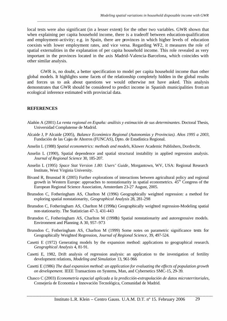
Modeling spatial variations in household disposable income with GWR __________________________________________________________________________________________
Instituto L.R. Klein – Centro Gauss. U.A.M. D.T. nº 15. February 2006
29
local tests were also significant (in a lesser extent) for the other two variables. GWR shown that when explaining per capita household income, there is a tradeoff between education-qualification and employment-activity; e.g. in Spain, there are provinces in which higher levels of education coexists with lower employment rates, and vice versa. Regarding WF2, it measures the role of spatial externalities in the explanation of per capita household income. This role revealed as very important in the provinces located in the axis Madrid-Valencia-Barcelona, which coincides with other similar analysis. GWR is, no doubt, a better specification to model per capita household income than other global models. It highlights some facets of the relationship completely hidden in the global results and forces us to ask about questions we would otherwise not have asked. This analysis demonstrates that GWR should be considered to predict income in Spanish municipalities from an ecological inference estimated with provincial data. REFERENCES
Alañón A (2001) La renta regional en España: análisis y estimación de sus determinantes. Doctoral Thesis, Universidad Complutense de Madrid.
Alcaide J, P Alcaide (2005), Balance Económico Regional (Autonomías y Provincias). Años 1995 a 2003, Fundación de las Cajas de Ahorros (FUNCAS), Dpto. de Estadística Regional.
Anselin L (1988) Spatial econometrics: methods and models, Kluwer Academic Publishers, Dordrecht.
Anselin L (1990), Spatial dependence and spatial structural instability in applied regression analysis. Journal of Regional Science 30, 185-207.
Anselin L (1995) Space Stat Version 1.80: Users’ Guide, Morgantown, WV, USA: Regional Research Institute, West Virginia University.
Bivand R, Brunstad R (2005) Further explorations of interactions between agricultural policy and regional growth in Western Europe: approaches to nonstationarity in spatial econometrics. 45th Congress of the European Regional Science Association, Amsterdam 23-27 August, 2005.
Brunsdon C, Fotheringham AS, Charlton M (1996) Geographically weighted regression: a method for exploring spatial nonstationarity, Geographical Analysis 28, 281-298
Brunsdon C, Fotheringham AS, Charlton M (1998a) Geographically weighted regression-Modeling spatial non-stationarity. The Statistician 47-3, 431-443
Brunsdon C, Fotheringham AS, Charlton M (1998b) Spatial nonstationarity and autoregressive models. Environment and Planning A 30, 957–973
Brunsdon C, Fotheringham AS, Charlton M (1999) Some notes on parametric significance tests for Geographically Weighted Regression, Journal of Regional Science, 39, 497-524.
Casetti E (1972) Generating models by the expansion method: applications to geographical research. Geographical Analysis 4, 81-91.
Casetti E, 1982, Drift analysis of regression analysis: an application to the investigation of fertility development relations, Modeling and Simulation 13, 961-966
Casetti E (1986) The dual expansion method: an application for evaluating the effects of population growth on developement. IEEE Transactions on Systems, Man, and Cybernetics SMC-15, 29-39.
Chasco C (2003) Econometría espacial aplicada a la predicción-extrapolación de datos microterritoriales, Consejería de Economía e Innovación Tecnológica, Comunidad de Madrid.

Modeling spatial variations in household disposable income with GWR __________________________________________________________________________________________
Instituto L.R. Klein – Centro Gauss. U.A.M. D.T. nº 15. February 2006
30
Chasco C, López F (2004) Modelos de regresión espacio-temporales en la estimación de la renta municipal: el caso de la Región de Murcia, Estudios de Economía Aplicada 22-3, 605-629
Cliff AD, Ord JK (1981) Spatial Processes: Models and Applications, Pion, London.
Cleveland WS (1979) Robust locally weighted regression and smoothing scatterplots. Journal of the American Statistical Association 74, 829-836.
Cravo JM, Ramajo J., Márquez MA (2004) Estimação de variáveis económicas sujeitas a dependências espaciais: o caso dos municípios de Portugal Continental, Revista Portuguesa de Estudos Regionais 5, 57-78
Cuadrado JR, Mancha T, Garrido R (1998) La convergencia regional en España: Hechos, tendencias y perspectivas. Fundación Argentaria-Visor, Madrid.
Eckey HF, Kosfeld R, Türck M (2005) Regional Convergence in Germany. A Geographically Weighted Regression Approach. Volkswirtschaftliche Diskussionsbeiträge 76/05, University of Kassel, Institute of Economics
Fingleton B (1999) Spurious spatial regression: some Monte Carlo results with a spatial unit root and spatial cointegration. Journal of Regional Science 39, 1-19
Florax R, Folmer H, Rey SJ (2003) Specification searches in spatial econometrics: the relevance of Hendry’s methodology. Regional Science and Urban Economics 33, 557–579
Foster SA, Gorr WL (1986) An adaptive filter for estimating spatially varying parameters: Application to modeling police hours spent in response to calls for service. Management Science 32, 878–889
Fotheringham AS, Brunsdon C (1999) Local forms of spatial analysis. Geographical Analysis 31, 340-358.
Fotheringham AS, Brunsdon C and ME Charlton (1998) Geographically weighted regression: a natural evolution of the expansion method for spatial data analysis. Environment and Planning A, 30, 1905-1927.
Fotheringham AS, Brunsdon C, Charlton M (2000) Quantitative geography. Sage, London
Fotheringham AS, Brunsdon C and Charlton M (2002) Geographically Weighted Regression. John Wiley and Sons, Chichester, UK.
Fotheringham AS, M Charlton and C Brunsdon (1997) Measuring spatial variations in relationships with Geographically Weighted Regression. In Fischer M, A Getis (eds), Recent development in spatial analysis. Springer-Verlag, Berlín, 60-82.
Fotheringham AS, M Charlton and C Brunsdon (2001) Spatial variations in school performance: a local analysis using geographically weighted regression. Geographical & Environmental Modelling 5-1, 43-66
Garrido, R. (2002) Cambio Estructural y Desarrollo Regional en España, Madrid, Spain: Pirámide.
Getis A, J Ord (1992) The analysis of spatial association by use of distance statistics. Geographical Analysis 24, 189-206.
Gorr WL, Olligschlaeger AM (1994) Weighted spatial adaptive filtering: Monte Carlo studies and application to illicit drug market modeling. Geographical Analysis 26, 67–87
Griffith DA (1978) A spatially adjusted ANOVA model, Geographical Analysis, 10, 296-301.
Griffith DA (1992) A spatially adjusted N-way ANOVA model. Regional Science and Urban Economics 22, 347-369.
Huang Y, Leung Y (2002) Analysing regional industrialisation in Jiangsu province using geographically weighted regression. Journal of Geographical Systems 4, 233–249
Hurvich CM, Simonoff JS, Tsai CL (1998) Smoothing parameter selection in non-parametric regression using an improved Akaike information criterion. Journal of Real State Society, Series B (Statistic Methodology) 60(2), 271–293
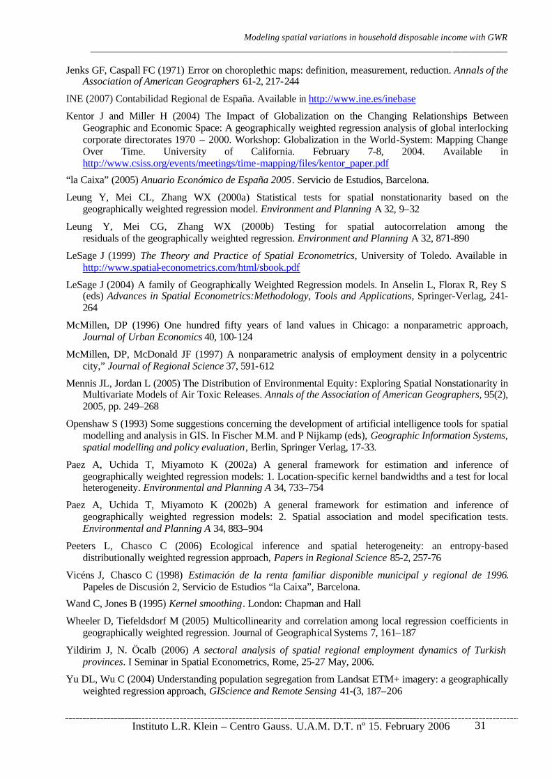
Modeling spatial variations in household disposable income with GWR __________________________________________________________________________________________
Instituto L.R. Klein – Centro Gauss. U.A.M. D.T. nº 15. February 2006
31
Jenks GF, Caspall FC (1971) Error on choroplethic maps: definition, measurement, reduction. Annals of the Association of American Geographers 61-2, 217-244
INE (2007) Contabilidad Regional de España. Available in http://www.ine.es/inebase
Kentor J and Miller H (2004) The Impact of Globalization on the Changing Relationships Between Geographic and Economic Space: A geographically weighted regression analysis of global interlocking corporate directorates 1970 – 2000. Workshop: Globalization in the World-System: Mapping Change Over Time. University of California. February 7-8, 2004. Available in http://www.csiss.org/events/meetings/time-mapping/files/kentor_paper.pdf
“la Caixa” (2005) Anuario Económico de España 2005. Servicio de Estudios, Barcelona.
Leung Y, Mei CL, Zhang WX (2000a) Statistical tests for spatial nonstationarity based on the geographically weighted regression model. Environment and Planning A 32, 9–32
Leung Y, Mei CG, Zhang WX (2000b) Testing for spatial autocorrelation among the residuals of the geographically weighted regression. Environment and Planning A 32, 871-890
LeSage J (1999) The Theory and Practice of Spatial Econometrics, University of Toledo. Available in http://www.spatial-econometrics.com/html/sbook.pdf
LeSage J (2004) A family of Geographically Weighted Regression models. In Anselin L, Florax R, Rey S (eds) Advances in Spatial Econometrics:Methodology, Tools and Applications, Springer-Verlag, 241-264
McMillen, DP (1996) One hundred fifty years of land values in Chicago: a nonparametric approach, Journal of Urban Economics 40, 100-124
McMillen, DP, McDonald JF (1997) A nonparametric analysis of employment density in a polycentric city,” Journal of Regional Science 37, 591-612
Mennis JL, Jordan L (2005) The Distribution of Environmental Equity: Exploring Spatial Nonstationarity in Multivariate Models of Air Toxic Releases. Annals of the Association of American Geographers, 95(2), 2005, pp. 249–268
Openshaw S (1993) Some suggestions concerning the development of artificial intelligence tools for spatial modelling and analysis in GIS. In Fischer M.M. and P Nijkamp (eds), Geographic Information Systems, spatial modelling and policy evaluation, Berlin, Springer Verlag, 17-33.
Paez A, Uchida T, Miyamoto K (2002a) A general framework for estimation and inference of geographically weighted regression models: 1. Location-specific kernel bandwidths and a test for local heterogeneity. Environmental and Planning A 34, 733–754
Paez A, Uchida T, Miyamoto K (2002b) A general framework for estimation and inference of geographically weighted regression models: 2. Spatial association and model specification tests. Environmental and Planning A 34, 883–904
Peeters L, Chasco C (2006) Ecological inference and spatial heterogeneity: an entropy-based distributionally weighted regression approach, Papers in Regional Science 85-2, 257-76
Vicéns J, Chasco C (1998) Estimación de la renta familiar disponible municipal y regional de 1996. Papeles de Discusión 2, Servicio de Estudios “la Caixa”, Barcelona.
Wand C, Jones B (1995) Kernel smoothing. London: Chapman and Hall
Wheeler D, Tiefeldsdorf M (2005) Multicollinearity and correlation among local regression coefficients in geographically weighted regression. Journal of Geographical Systems 7, 161–187
Yildirim J, N. Öcalb (2006) A sectoral analysis of spatial regional employment dynamics of Turkish provinces. I Seminar in Spatial Econometrics, Rome, 25-27 May, 2006.
Yu DL, Wu C (2004) Understanding population segregation from Landsat ETM+ imagery: a geographically weighted regression approach, GIScience and Remote Sensing 41-(3, 187–206

Modeling spatial variations in household disposable income with GWR __________________________________________________________________________________________
Instituto L.R. Klein – Centro Gauss. U.A.M. D.T. nº 15. February 2006
32
Yu D-L (2006) Spatially varying development mechanisms in the Greater Beijing Area: a geographically weighted regression investigation, The Annals of Regional Science 40-1, 173-190.