modelling settlement location in the troad using
TRANSCRIPT

MODELLING SETTLEMENT LOCATION IN THE TROAD USING GEOGRAPHIC
INFORMATION SYSTEMS.
By
Dominick Kevin Del Ponte
Submitted to the Faculty of
The Archaeological Studies Program
Department of Sociology and Archaeology
In partial fulfillment of the requirements for the degree of
Bachelor of Science
University of Wisconsin-La Crosse
2013

i
Copyright © 2013 by Dominick Kevin Del Ponte
All Rights reserved

ii
MODELLING SETTLEMENT LOCATION IN THE TROAD USING GEOGRAPHIC
INFORMATION SYSTEMS.
Dominick Del Ponte, B.S,
University of Wisconsin-La Crosse, 2013
The Hellenic period began around 2,700 years ago in the Troad. This was followed after a short
period of turmoil by the Hellenistic around 2,200 years ago. These periods are characterized by
the introduction of Greek culture and colonization. Many of these colonial sites have been
discovered in recent archaeological survey. Despite this, the settlement data is still incomplete.
It is the goal of this study to assist in the locating of Hellenic and Hellenistic sites through the
creation of a predictive model using GIS. This model has made evident the need to continue
exploration of the Troad.

iii
ACKNOWLEDGEMENTS
Thank you to: My instructor Dr. Joseph A. Tiffany. My faculty readers Dr. Mark Chavalas and
Dr. Gargi Chaudhuri. My student readers Marianna Clair and Megan Lorence. Dr. Peter
Jablonka, and Dr. William Aylward for providing data sets.

1
INTRODUCTION
When investigating an area for archaeological significance a series of steps must be taken,
in,attempt to not only locate sites but also to determine how they relate to each other. Often
these steps include historical research, ethnographic research, and general survey practices.
While these methods are effective in locating sites, they can be exorbitantly costly and incredibly
time consuming due to the amount of ground that needs examining. The prohibitive cost of
survey work may also lead to a certain amount of archaeological bias in a region. Survey bias
can effectively distort the glimpse into the past that archaeologists are attempting to garner. The
primary cause of this bias is the lack of time and funds to run full survey work based on regional
sample designs. Thus, the choice must often be made to survey either around a known site or to
survey in a location that has no guarantee of uncovering anything, leading to lost time and
money.
An example of this bias would be the Troad. The Troad is roughly outlined by the
modern day Turkish province of Çanakkale as highlighted in Figure A1. The extent of the Troad
has never been precisely established, however, it is loosely defined by the Greek geographer
Strabo as the area seen in Figure A2. This area was occupied by the Hellenic and Hellenistic
people from roughly 700 B.C. to 146 B.C. when the Romans captured the region. The potential
survey bias in the region comes from the area around the City of Troy. Due to Troy’s high
visibility, the immediate vicinity has been the focus of more extensive survey than the
surrounding areas of the Troad. The more intensive survey of the immediate area around Troy
has led to a higher density of sites directly surrounding Troy than the rest of the Troad.

2
This study examines archaeological bias in the Troad as well as predicts where unknown
settlements may be. This was done using Geographic Information System (GIS) to take into
account several variables that may have played into settlement location decisions by the Hellenic
and Hellenistic peoples. Using GIS, I developed a predictive model to illustrate areas of high
probability thereby narrowing the areas that are in need of survey.
BACKGROUND
The Hellenic and Hellenistic periods were characterized by Greek coastal cities that until 427
B.C. were under the rule of the Mitylene’s from the isle of Lesbos (Cook 1973:360). The exact
date that Greek occupation began is under debate; some authors claim to have evidence of
occupation pre-700 B.C. (Cook 1973:361). Despite this, settlement occupation of Asia Minor
began around 7400 B.C. shown through the site of Çatalhöyük (Fairbarn 2010:202). While
Çatalhöyük is within Asia Minor, it is not in the Troad. However, it lends credence to the idea
that the Troad had continuous occupation for thousands of years before the Greek arrival. The
continual occupation of the Troad created a blending of people and social structure in the early
Hellenistic period as Greek city life entered the Troad. The social structure changes required the
local people to adjust to a slightly different way of living from their own as the concentration of
people increased. Due to settling from Greece most of the cities developed along the coast. The
primary coastal settling created a network of cities that had high density near the coast but were
more spread-out inland (Cook 1973:363). This spreading is believed to have allowed Hellenic
people the full control of nearly all of the land in the area. Despite this control the cities,

3
especially inland, were isolated allowing them to easily fall into the hands of tyrants and
dynasties until the end of the fourth century when the Hellenistic period began (Cook 1973:363).
Hellenistic Period
Until 427 B.C., the cities within the Troad fell under control of the Mitylene followed by the
control of Athens. Athen’s rule was rebuked by the local dynasty of Zenis and Mania of
Dardanos. The loss of control from Athens created a period of instability in the fourth century,
as there was no longer a league of cities to offer protection from the myriad of warlords. This
period of turmoil ended in 334-332 B.C. when Alexander liberated the Greek cities. At this time,
nearly 20 cities sprang up in celebration of their freedom. Despite under Greek control once
again, there was still only roughly 100,000 people in the rather larger area of the Troad (Cook
1973:64). This rather low population was a problem for them, as they could not defend
themselves against the warlords that were still in the region, and they had little to no political
influence.
The multitude of small cities were not considered viable independent units. Therefore,
Antigonus “the one eyed” began combining many of these smaller cities into larger more viable
political units. Antigonus was the Satrap of Greater Phrygia that included the Troad. He was
placed as Satrap in 333 B.C. by Alexander as he conquered Asia Minor (Anson 1988:471). The
condensing of the population undertaken by Antigonus may have been to not only increase the
viability of these cities in the political arena but also allowed them to be easily defended as
Phrygia contained Alexander’s vital supply line back to Greece as he pressed further east. This
supply line was under near constant threat from the Persians navy until its surrender during the
siege of Tyre (Anson 1988:473).

4
METHODOLOGY
This analysis is based upon the use of GIS processes that allows for the creation of maps
compiled from various sources of data to visualize and interpret the issues of settlement pattern
discrepancies and survey bias within the Troad.
Geographic Information Systems (GIS)
GIS is a powerful computational method to examine the spatial relationship among data through
the creation of maps where real world objects are virtually reconstructed through points,
polygons, and lines. These objects may range from population to vegetation to elevation and
much more. In addition to analyzing single entities, GIS are capable of analyzing multiple forms
of data including spatial, temporal, and statistical components. When these components are used
together, they allow for the creation and visual representation of data to illustrate what is
happening in a region. There iarea myriad of GIS programs available, this project uses the
highly regarded ArcMap 10.1 produced by ESRI, was utilized for this study.
The following summary of GIS is derived from Longley et al. 2011. GIS processing
systems use data in primarily two forms: raster and vector. Raster data is used to show
continuous features such as slope and vegetation, as well as being the format of all images.
Raster data is composed of a series of cells formatted in a grid structure. This grid formation
allows for a binary yes or no system to be used as every cell may only have one trait. While
raster data uses cells and grids to denote land features, vector data is composed of a series of
nodes and arcs that are connected to form the geographic features. Vector data’s use of lines and

5
nodes allows it to represent accurately the location of discrete features such as streams, roads,
pipes, and other system networks. Both raster and vector data are stored within the GIS as a
single operable feature. For the purposes of this study, a mix of vector and raster data was
utilized depending on the feature that is being addressed.
After the data has been assembled and depicted in either raster or vector format a series
of processes may be run depending on the data format. Buffer distance is the establishment of
concentric rings emanating from a central shape such as riverbed or archaeological site location.
The buffer distance allows these areas to be classified by probability dependent on their distance
from the given object.
A group of similarly classified layers within GIS may be overlain on each other to show
where all of the buffer probabilities are the highest. The data buffering can then allow for the
statistical analysis of the probability zones to show the chance of a site being located within the
zones shown upon the overlay map.
Georeferencing
In order to understand some of the processes used to compile the data for this project, an
understanding of the concept of georeferencing is important. Georeferencing is defined as “the
assigning of a unique location to atoms of information” (Longley et al. 2011:124). This is the
taking of pieces of information that are not spatially located and giving them the same fixed
locational references. In order to ensure quality and ease of use, georeferencing has three
principle rules; that all points are unique, that the meaning of the reference is shared to all, and
that the points used to georeference are temporally stable. These rules are important to avoid
distortion of the map as well as confusion about the location being referenced due to duplicate
potential reference points such as city names as well as the landscape changing over time.

6
Recent GIS in Archaeology
Predictive modeling in archaeology via GIS has been done with great success recently as can be
seen through the modeling work done by Melanie Riley in Mills County Iowa where she created
a seven variable predictive model for earth lodge sites that yielded 71% accuracy (Riley 2010).
While both Mills County Iowa and the Troad are relatively easy areas to survey predictive,
modeling is very useful in areas of harsh terrain. GIS predictive modeling has been used to
predict the locations of site in the jungles of Belize. The modeling done in Belize was a six
variable model that predicted with and accuracy of 75%. Models such as this have allowed for
the discovery of previously unknown sites because of the narrowing of the survey areas (Ford et
al. 2000).
Projection and Datum
As part of georeferencing raster data and to maintain accuracy throughout the creation of the
model, a standard for projection must to be established. The projection and datum used for this
study is the WGS 1984 projection and datum. This projection was chosen because it is the most
universally accepted format for cartography today. A standardized projection and datum is
necessary in order to maintain uniformity within the mapping and to allow for easier sharing of
data between cartographers as a known and standardized projection allows for easier access and
understanding of the map.

7
Data Collection and Parameters
Settlement Locations
The known settlement locations in the Troad were provided by Dr. Peter Jablonka (Aslan et al.
2012). The points in Figure A3 represent all Hellenic and Hellenistic sites in the Troad ranging
from settlements to forts to trading outposts. The settlement locations are represented by vector
data points.
Water Bodies
The establishment of water bodies is a critical step in analyzing the settlement locations of the
region. This was done by georeferencing multiple maps to extract as much information as
possible while allowing for the crosschecking of the older maps to help insure the accuracy.
After georeferencing, a feature layer representing the water bodies was digitized by tracing the
visible features to develop the map as depicted in Figure A4. The larger permanent bodies of
water such as lakes were already digitized by the Natural Resource Department of Turkey. One
water aspect not represented is the presence of small springs or wells such as the springs under
the wall of Troy as described by Homer (Strabo1923:200). This is due to the data not being
present for small temporally short springs or streams two thousand years ago.
Slope
The slope data seen in Figure A5 has been extracted from the Shuttle Radar Topography Mission
(SRTM) conducted in 2000. The SRTM data has a 3-meter resolution.

8
Soils
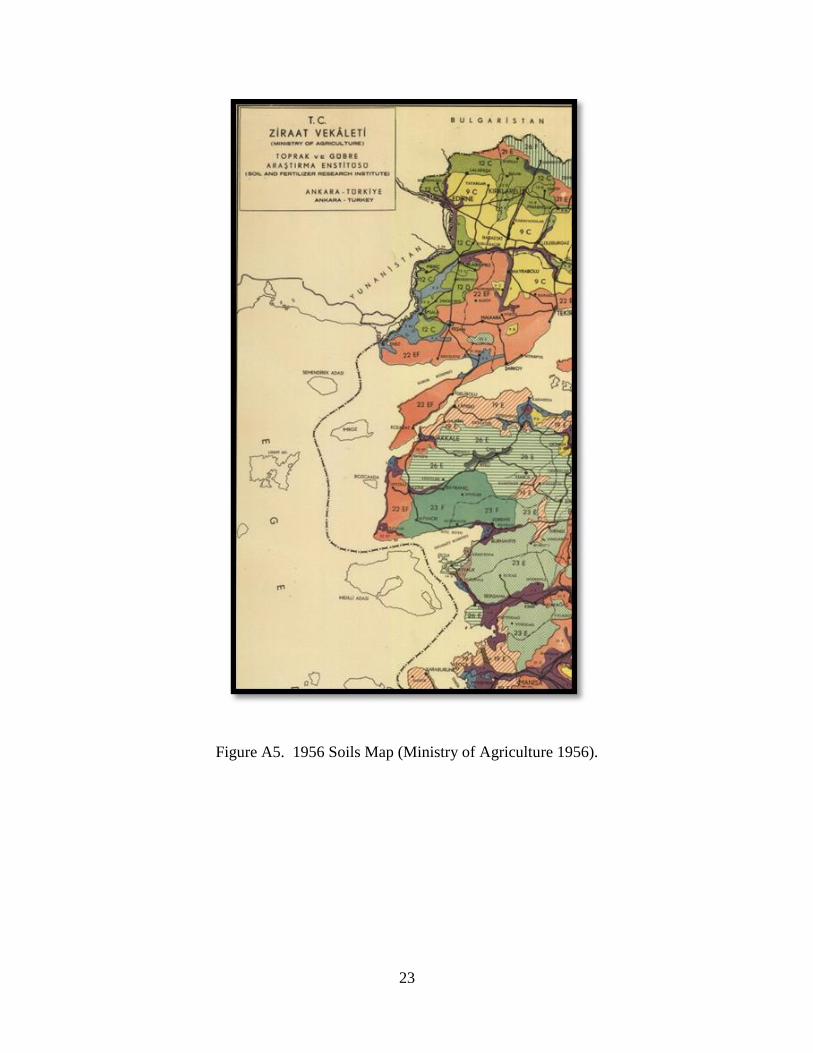
The soils of the region were surveyed in 1956 by the Turkish Ministry of Agriculture. The map
in Figure A6 is the 1956 map that was used as the base map for the soil layer. The survey broke
the region into seven distinct soil categories. These seven categories in order of fertility are
hydromorphic saline soil (shown in blue), developed under the once paleo-sea of the Trojan
plateau. Alluvial and youthful soils (shown in purple) are relatively new and fertile soils created
through decomposition of organics or the movement of material through alluvial (windblown)
processes. Noncalcic brown rendzina soil material (shown in red) is lacking in calcium and soil
depth creating a rather acidic and shallow soil that is not as hospitable to all plant life as the
previously mentioned types (Lal 2002:1127). Brown forest and podzolic soil material (shown in
horizontal green bands), is of lesser fertility due to the inherently low fertility of forest soils (Lal
2002:587). Terra Rosa soil material (shown in red diagonal bars) is a shallow clay rich material.
Brown forest soil (shown in green) is also lacking in fertility due to the low water holding
capacity of forest soil (Lal 2002:587). Moderately sloping rendzina soil material (shown in grey)
has higher erosional rate due to its shallow depth and slope making it less suitable for agriculture
(Lal 2002:1127).
Coastline
The nature of the Hellenic and Hellenistic people being sea faring people as well as relying upon
trade from Greece for many things made them more apt to settle along the coast. Therefore, the
coast provides a critical component within this analysis. The coastline was created through the
georeferencing of satellite imagery.

9
Data Processing
The data processing is fashioned in such a way to provide five categories to each parameter
stated above. The categories are based on distance to water, soil fertility, and degree of slope.
The categories are highly probable, somewhat probable, moderately probable, somewhat
improbable, and improbable. This categorization is done so that the maps may be overlaid on
each other to show the high probability zones when every variable is taken into account.
Settlement Locations
The settlement locations received a buffer of 1km increments extending outward to 4km after
which all distance is given the same weight. The 1km buffer distance seen in Figure A7
represents the catchment distance or the area from which a settlement will draw the majority of
its resources. Due to the catchment, distance required for site stability the area furthest away
from neighboring settlements is considered to be of the highest probability. Despite the arbitrary
catchment buffer only six sites fall within the somewhat improbable and improbable categories
placing 82% of all sites within moderately probable to highly probable.
Water Bodies
The water bodies were given a buffer in 1km increments extending out to 4km after which
everything is grouped as one. These distances were used because 1km is roughly a thirty-minute
walk, allowing for relatively easy access to fresh water Figure A8 shows this buffer distance of
streams in relation to known sites showing that 90% of all sites fall within 2km of a river or
within the higher groups of probability. Figure A8 does not include the lakes although the layer
is present in the final overlay seen later. Lakes have been given the same buffer as streams. This
layer does not take into account the location of springs and temporally short streams.

10
Slopes
The 0-90° slopes have been broken into five natural interval segments. Natural interval is a
computation that allows for the greatest degree of variability between the classes while grouping
the items of highest similarity together. Since the natural interval computation of the data, is
done via computer, user bias is eliminated from this stage. The intervals give lesser slopes a
higher degree of probability while assigning steeper slopes a lower probability. The
reclassification gave favorability areas of lesser slope that would be more evident of fertile plains
than the steeper areas of more rocky topography as seen in Figure A9. Approximately 75% of
sites are located within the highly probable and somewhat probable ranges.
Soils
The seven soil types were condensed into five categories based on their fertility. Figure A10
demonstrates this as brown forest and podzolic soil material, brown forest soil in mountainous
terrain and moderately sloping rendzina soil material were grouped into a single unfavorable
category. After reclassifying 54% of sites fall within the highly probable or somewhat probable
categories.
Forests
The original seven soil layers have been reclassified into five forest layers. This was done based
on if the soil in the region showed evidence of a forest environment at some point in the past.
This method has been done because the modern forested areas are likely to not have been the
forested areas in the Hellenic and Hellenistic periods. This process created the map as seen in
Figure A11. The forest layer contains 64% of all sites within highly probable or somewhat
probable.

11
Coastline
As stated earlier the coast is an important feature in the landscape of the Hellenic and Hellenistic
people of the Troad. With that in mind, the coastline as seen in Figure A12 has been given a
3km interval buffer up to 10 kilometers after which everything is grouped. This has been done
due to the connection with Europe and the known sites showing a trend within 3km of the coast.
Despite this connection, only 57% of settlements are within 3km of the coast.
Overlay and Summary
The final stage of the modeling process is to overlay all of the previously shown layers on a
single map. This is done through a weighted sum of all of the layers. What is done in a
weighted overlay is the combination of the previously mentioned layers into a single entity. All
of the created layers have the same scaling from highest probability to lowest probability in order
to maintain a uniform scale for the overlay process. This process allows the six layers to be
placed one on top of the other to highlight the areas of high probability they all have in common.
While this process is easy to visualize it involves many complex calculations to be run by the
GIS in order to maintain accuracy within the map as the maps are overlaid. In addition to
placing the maps on top of each other, a weighted sum will give more weight to layers as
specified increasing how they affect the outcome. The weights given to the six layers were
based upon the probabilities described earlier. These percentages where placed into the weighted
sum giving water (lakes and streams) a 0.90 weight while soils had a 0.54 weight, coastline was
given 0.54 weight, slope was given a 0.75 weight, known settlement were given a 0.82 weight,
and forests were given a 0.64 weight. This differential weighting gives the map more accuracy
as geographic features that are of higher probability will a greater impact on the result. In order
to help conceptualize the parameters they have been summarized in Table 1.

12
Table1. Summarization of geographic parameters used.
Class Highest
Probability
High
Probability
Neutral Low
Probability
Lowest
Probability
Distance to
sites
>4 km 3-4 km 2-3 km 1-2 km 0-1 km
Soil fertility Hydromorphic
Saline
Alluvial and
Youthful
Non-Calcic
Brown
Rosa Terra Other
Distance to
water
< 1 km 1-2 km 2-3 km 3-4 km >4 km
Distance to
coast
<3 km 3-6 km 6-9 km 9-12 km >12 km
Percent rise
of slope
Natural intervals determined by computer based upon the percent rise. Steeper
slopes given lower values, flatter plains given higher values.
Buffering Bias
In order to examine the archaeological bias within the Troad directly related to the area
surrounding Troy that is currently distorting the settlement distribution seen earlier an arbitrary
20km buffer ring has been placed around Troy. The ring is cropped to the coastline to allow for
more visual clarity of the subject matter. This buffer shows that 54% of all known sites are with
20km of Troy. While this may be explained through importance of the City of Troy in the
Troad, it is unlikely as seen in Figure A13.

13
ANALYSIS AND RESULTS
Testing the Model
The model is created through a map overlay. In order to test the model the environmental
parameters were run without the known settlements catchment buffers as seen in Figure 1. The
model predicts within 75% accuracy for known settlements falling within the high or somewhat
probable classifications. However, there is a slight geographic anomaly to the southeast of Troy
where the once paleo-sea of the Trojan plateau ended. This anomaly is where the Scamander
Valley cuts through a small-elevated region that contains a different soil type than the
surrounding area. The area that is different in soil type is also topographically different from the
rest of the Scamander valley. The majority of the Scamander Valley is as traditional flat river
basin while this area is a steep and rocky environment. The small stretch of the Scamander that
has incised through this area has four sites on its banks. While this is an important grouping of
sites, if they are excluded as anomalous, the model predicts with 86% accuracy. This is not
perfect but allows for a decent understanding of where unknown settlements may be located.

14
Figure 1. Testing the Model.

15
Analyzing the Model
The model as seen in Figure 2 shows that while there still are some locations of high probability
within the 20km buffer around Troy there is more area of high site probability located in other
regions. Figure A14 demonstrates this by inserting the 20km bias buffer as a negative parameter
to the map. This is done to highlight the area that should be avoided in survey work, as much of
what is there is likely to have been discovered. The density of the high probability is primarily
along the coast specifically the Northwestern coast as well as the Southwestern coast as the
coastal area between is already extensively covered. In addition, some of the inland areas along
Scamander river valley are also of higher probability.

16
Figure 2 Completed Model.

17
DISCUSSION AND CONCLUSIONS
The processes involved in the creation of the model provides adequate data for further processes
to be run and allows enough flexibility within the model for additional parameters to be added.
The addition of more parameters may alter the accuracy of the model but should not have a great
effect on the probability areas. The model has shown three distinct areas of interest, the
northwest coast, the southwest coast, and the inland areas. Each area is distinct in the processes
that may be causing the presence or lack of sites in relation to the models probability zones.
The Northwest Coast
The Northwest coast is particularly interesting because of the location of contemporaneous sites
on the Gallipoli peninsula located just 1.2-6 km on the other side of the Dardanelles. If these site
locations are taken into account, a correlation may be able to be drawn between these known
sites and high probability zones on the eastern side of the Dardanelles. While this is speculative
perhaps a sister port city model may become apparent with further exploration of the eastern
side.
The Southwest Coast
Unlike the northwest coast, the southwest coast does not have any directly relating settlements
that may lead to yet further increased probability. Despite this there are a few areas of distinctly
high probability shown in purple that should be examined for potential sites particularly due to
their relation to larger flowing water sources in the region and there relatively close proximity to
the Greek mainland.

18
Inland
The inland area does not show the very high probability that the coastline does. However, for
inland survey, it appears that looking in the transitional areas between the fluvial plains of the
Scamander and its tributaries and the surrounding colluvial toe slopes may be recommended as
the few known inland sites are located within this transitional area.
Suggestions for Further Research
The addition of more environmental attributes to the model may prove to be useful as it would
refine and hone the accuracy. However, ground proofing the model may be the next step in
order to demonstrate the validity of the model. This may be done through any of the classical
survey technique or through remote sensing techniques. For both statistically representative
sampling methods are recommended to increase data applicability statistically and enhance
future modeling efforts.

19
APPENDIX
MAPPING
Figure A1. Overview of Modern Turkey, Canakalle Province Circled. (nationsonline 2012)

20
Figure A2 Strabo’s Troad. (Strabo 1923)

21
Figure A3. Known Hellenic and Hellenistic Sites in the Troad.

22
Figure A4. Modern Streams in the Troad.
23
Figure A5. 1956 Soils Map (Ministry of Agriculture 1956).

24
Figure A6. Topography of the Troad.

25
Figure A7. Stream Buffer.

26
Figure A8. Soil Classification extracted from the 1956 Soil Map, Figure A5.

27
Figure A9. Forest Soils Extracted from 1956 Soil Map, Figure A5.

28
Figure A10. Survey Bias.

29
Figure A11. Model With Bias.

30
BIBLIOGRAPHY
Aslan, Rüstem, Gebhard Bieg, and Peter Jablonka
2012 Unpublished data set for Prehistoric sites in the Troad. On file, Universität
Tübingen, Germany.
Cengiz, D.
2000 General Directorate of Mineral Research and Exploration. Electronic document
http://www.mta.gov.tr/v2.0/eng/maps.php?id=metallogeny, accessed February 4,
2013.
Cook, J.M.
1973 The Troad: An Archaeological and Topographical Study. Oxford University
Press, New York.
Fairbairn, Andrew
2005 Garden Archaeology. World Archaeology 37 2:197-210.
Ford, Annabel, Clark Wernecke, Jose Manuel Chavez, Rudy Larios, and William C. Poe
2000 Assessing the Situation at El Pilar: Chronology, Survey, Conservation and
Management Planning for the 21st century BRASS/EL PILAR Field Reports,
MesoAmerican Research Center, Institute for Social, Behavioral and Economic
Research, UC Santa Barbara.
Gale, N. H., Z. A. Stos-Gale, and G. R. Gilmor
1985 Alloy Types and Copper Sources of Anatolian Copper Alloy, Anatolian Studies
35:144-173.
Gates, Marie-Henriette
1996 Archaeology in Turkey, American Journal of Archaeology 100:2:277-335.

31
Hormann, Christopher
2012 View Finder Project. Elevation model
http://www.viewfinderpanoramas.org/Coverage%20map%20viewfinderpanorama
s_org3.htm, accessed February 13, 2013.
Lal, Rattan (editor)
2002 Encyclopedia of Soil Science. Marcel Dekker, New York .
Longley, Edward, Michael Goodchild, David Maguire, and David Rhind
2011 Geographic Information Systems and Science. John Wiley and Sons, New Jersey.
Nations Online
2012 Map the nations project. Electronic document, http://www.nationsonline.org/,
accessed April 15, 2013.
Ministry of Agriculture
1956 Soil and fertilizer research Institute. Electronic document
http://eusoils.jrc.ec.europa.eu/EuDASM/TR/TR_13001_01.jpg, accessed January
28, 2013.
Riley, Melody
2010 Chapter 6. Weights of Evidence Predictive Model for Earthlodge Sites in the
Glenwood Locality, Mills County, Iowa, In, Cultural Resources of the Loess
Hills: A Focus Study to Determine National Significance of Selected
Archaeological Cultural Resources Along the Loess Hills National Scenic Byway.
Edited by Melody K. Pope, Joseph A. Tiffany, Angela Collins and Michael J.
Perry. Contract Completion Report No. 1700, pages 6-100 Office of the State
Archaeologist of Iowa, Iowa City.
Strabo
1923 Strabo on The Troad. Translated by Walter Leaf. Cambridge University Press,
London.
