I hereby declare that, except where specifically indicated, the work submitted herein is my

own original work

Signed ………………………………………………………………………………………… Date …………….…………………

Modelling SCR Installation

by

Stephanie Mennecier (PET)

Fourth-year undergraduate project

In Group D, 2014/2015

2 | P a g e

Table of Contents 1 Technical Abstract .............................................................................................................. 3

2 Introduction ....................................................................................................................... 5

3 Background Theory ............................................................................................................ 7

3.1 Touchdown Zone ......................................................................................................... 7

3.2 Loading on an SCR ....................................................................................................... 8

3.2.1 Installation ........................................................................................................... 8

3.2.2 Working Life Loading ........................................................................................... 9

3.3 Overview of Modelling the Installation Process ....................................................... 10

3.3.1 Load-Displacement (𝑃, 𝑦) Model ....................................................................... 14

3.3.2 Beam-Spring Model ........................................................................................... 19

3.4 Harbour Test .............................................................................................................. 21

4 Results and Discussion ..................................................................................................... 24

4.1 Installation angle ....................................................................................................... 24

4.1.1 Effect of varying installation angle on trench depth ......................................... 24

4.1.2 Effect of varying installation angle on moment envelope ................................. 26

4.1.3 Combining installation and displacement loading ............................................ 27

4.2 Parametric Study ....................................................................................................... 30

4.2.1 Effect of varying riser diameter ......................................................................... 31

4.2.2 Effect of varying penetration rate ..................................................................... 33

4.3 Design Recommendations......................................................................................... 39

4.4 Critical Evaluation of the Model ................................................................................ 40

5 Conclusion ........................................................................................................................ 41

6 References ....................................................................................................................... 42

7 Appendices ....................................................................................................................... 44

7.1 Appendix 1: Risk assessment .................................................................................... 44

3 | P a g e

1 Technical Abstract

Fatigue stresses associated with extreme storms, vessel movements and vortex-induced

vibrations are critical to steel catenary riser (SCR) performance. The critical location for

fatigue damage is in the touchdown zone (TDZ); the region where cyclic interaction between

the riser and seabed occurs. As seafloor stiffness cannot be estimated with a great deal of

reliability, neither can the bending stresses and fatigue life of the risers.

Aubeny and Biscontin (2006) proposed a non-linear load-displacement (𝑃, 𝑦) model to

describe seafloor-riser interaction based on model testing. It considers the problem in terms

of a linearly elastic pipe resting on a bed of uncoupled non-linear springs and requires the

iterative solution of a fourth-order ordinary differential equation for the differential

displacement along the pipe, Δ𝑦. The load-displacement model can take account of non-linear

soil behaviour, suction and breakaway, yielding, and soil degradation under cyclic loading. It

requires a number of input parameters related to riser and soil properties.

One of the most critical loading scenarios within the TDZ occurs during installation. Three

additional model parameters are required to simulate it: the installation angle 𝜃 and the two

locations along the riser between which the installation loading will be applied, 𝑥1 and 𝑥2.

Installation loading is modelled by applying a rotation 𝜃 at the node 𝑥2 m along the riser and

determining the resultant deflected shape of the riser before updating all the state variables.

To simulate that the soil to the side of the rotation where the riser has been vertically

displaced remains untouched, the soil surface profile is reset to the riser’s self-weight

penetration depth. The rotation is then released and this process is repeated at each node in

turn between 𝑥1 and 𝑥2 until a full post-installation soil surface profile has been calculated.

Calibrating the model with field observations by Bridge and Willis (2002) and Bridge and

Howells (2007) allowed a realistic value of 𝜃 = 0.09 radians to be estimated. Further

simulations demonstrated that increasing the value of 𝜃 has the effect of increasing the post-

installation trench depth and moment envelopes of the riser during installation and

subsequent operational loading. This is because the shear strength profile of the soil, and

4 | P a g e

hence its resistance, increases with trench depth, inducing greater moments in the riser.

Consequently, this has a detrimental impact on the riser’s fatigue life and indicates that

current predictions neglecting installation loading may not be conservative.

A parametric study looking at the effect of the riser’s diameter and penetration rate on trench

depth and bending moments identified that increasing the riser’s diameter has a negative

effect on its fatigue life; however, increasing the penetration rate served to reduce the

maximum moments experienced by it and its working life. Despite the model being quasi-

static, the effect of penetration rate could be analysed by calibrating the degradation model

parameters with two large-scale NGI tested carried out at differing penetration rates. On

account of the observations drawn from the study, it is recommended that when installing

offshore risers, the installation angle is kept as shallow as possible and the riser diameter is

kept to a minimum to reduce moments both during installation and the working life of the

riser and increase the riser’s fatigue life.

In conclusion, installation has been shown to be one of the most critical loading scenarios

during the life of a SCR and modelling this scenario has enabled more realistic bending

moment and trench depth predictions along the riser which allows for improved fatigue life

estimates.

5 | P a g e

2 Introduction

As oil and gas production moves into deeper and deeper waters, new designs for riser pipes

have had to be developed. These pipes are used to transport oil from the well head on the

seafloor to the offshore floating structure. One of the most popular systems is the steel

catenary riser (SCR) system which was first used by Shell in 1994 (Mekha, 2001). The risers

are typically 0.2 - 0.35 m in diameter and operate at a pressure of 13.5 - 41.5 MPa (Howells,

1998).

Fatigue stresses associated with extreme storms, vessel movements and vortex-induced

vibrations are critical to SCR performance. The critical location for fatigue damage is in the

touchdown zone (TDZ); the region where cyclic interaction between the riser and seabed

occurs. The maximum bending stresses also typically occur in this section of the riser. They

are very are sensitive to seafloor stiffness such that an SCR will experience greater bending

stresses on rigid soil than on soft soil. At present, seafloor stiffness cannot be estimated with

a great deal of reliability and hence neither can the bending stresses and fatigue life of the

risers.

Despite linear elastic seafloor models providing useful insights (Pesce, et al., 1998), full scale

model tests (Bridge, 2002; Bridge 2004) have shown that the riser problem involves complex

nonlinear processes including:

Trench formation

Non-linear soil stiffness

Finite soil suction

Breakaway of riser from the seafloor

In addition, studies indicate that soil stiffness degradation effects can be significant when

dealing with cyclic loading of pipes on soil (Dunlap, 1990; Clukey, 2005) such as those

experienced by the riser in the TDZ.

In order to try and understand this behaviour further, Aubeny and Biscontin (2009) developed

a non-linear seafloor-riser interaction model in MATLAB which considers the problem in terms

of a linear elastic pipe resting on a bed of springs whose stiffness’ are described by non-linear

6 | P a g e

load displacement (𝑃-𝑦) curves. The problem is treated as quasi-static, disregarding the

inertia of the riser, and requires the iterative solution of a fourth order ordinary differential

equation by means of the finite difference method. The initial version of the model allowed

for virgin penetration, non-linear soil stiffness, soil suction and breakaway however it did not

take into consideration soil degradation. The model has since been developed by You (2012)

so that accumulated deflection during the loading of the soil serves as a measure of energy

dissipation in order to quantify soil degradation. Any combination of imposed vertical

displacements, tension and moments can be applied at one end of the riser however, lateral

motions of the riser have been neglected to simplify the analysis (despite evidence that they

can affect riser performance (Morris, 1988; Hale, 1992)), by assuming that they are less than

4 pipe diameters wide. This assumption also justifies the use of small-strain, small-deflection

beam theory.

Further improvements to the model, detailed in this report, involve the incorporation of

modelling riser installation. The motivation being that one of the most critical loading

scenarios occurs when the riser is installed, during which it undergoes large deformations

creating trenches several diameters deep (Bridge & Howels, 2007). The effect of these deep

post-installation trenches on the riser’s fatigue life is currently under dispute with some

authors reporting an decrease in fatigue damage due to trench formation (Bhat, et al., 2013 ;

Giertsen, et al., 2004) while other suggest that is detrimental to the fatigue life of the SCR

(Clukey, et al., 2007 ; Nakhaee & Zhang, 2008) . The current MATLAB model does not take

into account the installation process at all but rather assumes that the initial trench depth

before operational loading is applied is solely due to the self-weight of the riser. Therefore

modify the model to include the installation process will allow for more accurate predictions

of the bending moments the riser is subject to and its fatigue life.

7 | P a g e

3 Background Theory

3.1 Touchdown Zone

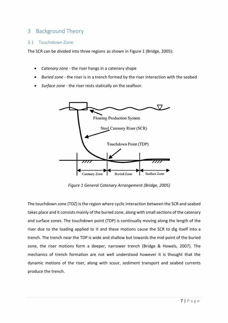
The SCR can be divided into three regions as shown in Figure 1 (Bridge, 2005):

Catenary zone - the riser hangs in a catenary shape

Buried zone - the riser is in a trench formed by the riser interaction with the seabed

Surface zone - the riser rests statically on the seafloor.

The touchdown zone (TDZ) is the region where cyclic interaction between the SCR and seabed

takes place and it consists mainly of the buried zone, along with small sections of the catenary

and surface zones. The touchdown point (TDP) is continually moving along the length of the

riser due to the loading applied to it and these motions cause the SCR to dig itself into a

trench. The trench near the TDP is wide and shallow but towards the mid-point of the buried

zone, the riser motions form a deeper, narrower trench (Bridge & Howels, 2007). The

mechanics of trench formation are not well understood however it is thought that the

dynamic motions of the riser, along with scour, sediment transport and seabed currents

produce the trench.

Figure 1 General Catenary Arrangement (Bridge, 2005)

8 | P a g e

3.2 Loading on an SCR

3.2.1 Installation

There are two main loading scenarios that an SCR is subject to during its lifetime. The first is

installation. There are two common methods of installing SCRs: the J-lay and S-lay methods,

so named due to the shape of the pipe during installation (Figure 2). The S-lay method is used

in shallow waters whereas the J-lay method is more suitable for deep water installations

where the water depth ranges between 400 - 1500 m. The reason for this is because, if used

in shallow waters, the J-lay method would require a departure angle near to the horizontal in

order for the pipe to fall in a catenary shape to the seabed. Rather, the optimum angle of

departure for the J-lay method is typically between 4 and 15 degrees to the vertical (2H

Offshore Engineering Ltd., 2006).

Some of the advantages and disadvantages of the J-lay technique over the S-lay are discussed

below (Callegari, 2005 ; Pulici, 2003 ; 2H Offshore Engineering Ltd., 2006).

Advantages:

Riser laid in a more natural configuration which allows for stresses to be kept well

within the linear elastic limit.

Figure 2 Deployment of marine pipelines by (a) the J-lay, and (b) the S-lay methods (Callegari & Lenci, 2005)

9 | P a g e

Reduction of the horizontal distance between the vessel and the touchdown point

which enables better positioning of the pipe – up to 1m accuracy.

Reduction of the horizontal force applied to the end of the riser by the vessel engines,

hence a lower lay tension.

Elimination of the section of the riser near the barge with high curvature which can

produce residual stresses.

Less susceptible to weather conditions.

Disadvantages:

Processing operations are more difficult along a steep ramp.

There is only space for a single joining station which can lead to slower laying rates.

Bigger vessels with more power are needed for dynamical positioning under all

operating conditions.

More expensive.

Good quality offshore welds are required in order to achieve sufficient fatigue lives.

3.2.2 Working Life Loading

The second loading scenario occurs during the SCR’s operating life when it typically hangs

from a floating oil platform and as such is subject to wave, current and wind loading. It

connects to the platform via either a flex joint or taper stress joint which transfer the dynamic

motions of the oil platform directly to the top of the SCR and cause the touchdown point

(TDP) to move along it. The main forms of dynamic motion are (Bridge, 2005):

First order motions – frequency motions caused by wave action on the platform

Second order motions – low frequency motions caused by swell waves and light

winds. Also known as slow drift motions

Static offset – displacement resulting from mean environmental loads such as

currents, waves and winds or system failures such as failed mooring lines

These motions result in cyclic loading on the seabed causing the riser to penetrate further

into the soil. This in-contact cycling of buried pipelines, where the pipeline does not lose

10 | P a g e

contact with the soil, has been written about by many authors including Dunlap et al. (1990).

They show that cyclic motion softens the seabed causing the soil stiffness to reduce as the

number of cycles increases.

3.3 Overview of Modelling the Installation Process

In their 2006 paper Aubeny and Biscontin proposed a non-linear load-displacement (𝑃, 𝑦)

model to describe seafloor-riser interaction inferred from model testing. It considers the

problem in terms of a linearly elastic pipe resting on a bed of uncoupled non-linear springs

(Figure 3) and requires the iterative solution of a fourth-order ordinary differential equation

for the differential displacement along the pipe Δ𝑦.

When simulating the installation of the riser, this seafloor-riser interaction model and the

solution of the governing differential equation are manipulated to determine the soil surface

profile after installation and its moment envelope during the procedure. The overall process

to achieve this is outlined in flow chart in Figure 4.

Figure 3 Spring-Pipe Model (Aubeny & Biscontin, 2006)

11 | P a g e

Firstly the soil and riser parameters are manually input along with three specific installation

parameters; the installation angle 𝜃, and the two locations along the riser between which

installation will be simulated, 𝑥1 and 𝑥2 (Figure 5). The self-weight penetration of the riser is

computed and acts as the baseline trench depth. Then a rotation, 𝜃, is applied at the node 𝑥2

m along the riser and the resultant deflected shape is assumed. This shape is then used to

calculate the soil resistance 𝑃 for each nodal spring and hence its secant stiffness 𝑘𝑠. Having

Figure 4 Flowchart outlining modelling of SCR installation process

12 | P a g e

estimated 𝑘𝑠 at each node, the governing differential equation for the riser can be solved

iteratively with appropriate boundary conditions by applying the central difference method

to calculate the true deflected shape before updating the state variables.

An example of the deflected shape of a 80m riser which has had a rotation applied to it at

50m along it length is shown in Figure 6. The trench depth to the left of where the rotation

was applied is then reset to the riser’s self-weight penetration (Figure 7) as during the real

installation process this soil would not have yet been disturbed.

Figure 6 Riser deflected shape due to applied rotation

𝑥2 𝜃 𝑥1 𝐿 Direction of trench formation

Figure 5 Installation parameters

13 | P a g e

The whole process is then repeated at each node between the locations 𝑥2 and 𝑥1 with the

rotation being released at the current node and being applied to the next (Figure 8) such that

a final post-installation soil surface profile is found as illustrated in Figure 9.

Figure 7 Trench depth reset to self-weight to the left of applied rotation

Figure 8 Trench forming as rotation is applied at each node along the riser

14 | P a g e

3.3.1 Load-Displacement (𝑃, 𝑦) Model

Each spring’s load-displacement (𝑃, 𝑦) characteristics follow the non-linear model illustrated

in Figure 10 that was developed by Aubeny and Biscontin (2006) where 𝑃 is the compressive

soil resistance and 𝑦 is the deflection of the riser into the soil. The model was based on the

observations of laboratory model tests of vertically loaded pipes in weak sediment (Dunlap et

al, 1990; Bridge et al, 2004). These tests indicated that significant soil suction occurs during

uplift before the riser begins to break away from the seafloor and that this process is not a

gradual one, hence the smooth curve between points B and C. Furthermore, when the

displacement of the riser reverses again at point C and reconnects with the seafloor, the soil

resistance is slowly mobilised as the riser penetrates the seafloor again. This is realised by the

S-shaped curve between points C and E.

Figure 9 Final trench depth profile due to installation

15 | P a g e

Overall, the 𝑃-𝑦 model in Figure 10 includes the following components which will be discussed

in more detail:

1. Virgin penetration into the seafloor characterised by the backbone curve (O-A)

2. A large deformation bounding loop (Path A-B-C-D-E) including elastic rebound with full

seafloor-riser contact (A-B), uplift with partial seafloor separation (B-C) and re-contact

and reloading (C-D-E) taking account of soil degradation.

3. Deflection and reversal from any arbitrary point along the bounding loop

4. Load cycles within the bounding loop

3.3.1.1 Backbone Curve

The backbone curve models the initial plastic penetration of the pipe into a virgin soil based

on the collapse load computations for a horizontal cylinder of diameter 𝐷 embedded in a

trench of depth 𝑦. The collapse load 𝑃 is related to the soil strength 𝑆𝑢 through a

dimensionless bearing factor 𝑁𝑝.

𝑃 = 𝑁𝑝𝑆𝑢𝐷 Equation 3.1

In the Aubeny and Biscontin model, an empirical power law function relates the bearing factor

𝑁𝑝 to trench depth 𝑦. This function (Equation 3.2) was developed by Aubeny, et al., (2005)

Figure 10 Degrading P-y Model (You, 2012)

16 | P a g e

where 𝑎 and 𝑏 are constants chosen to fit various conditions of penetration and pipe

roughness. It is valid for trench depths up to 𝑦 = 5𝐷 and takes into consideration a non-

uniform undrained shear strength profile of the form 𝑆𝑢 = 𝑆𝑢𝑜 + 𝑆𝑔𝑧 where 𝑆𝑢𝑜 is the

undrained shear strength at the surface of the seabed and 𝑆𝑔 is the shear strength gradient

with depth whose values typically range from 0-4 kPa and 0-20 kPa respectively for soft, silty

clays.

𝑁𝑝 = 𝑎 (𝑦

𝐷)

𝑏

Equation 3.2

Equation 3.2 only consider cases where the trench width, 𝑤, equals the trench diameter 𝐷. In

the case where 𝑤/𝐷 > 1 the maximum bearing resistance that can develop against the pipe

decreases. To take this into consideration, additional relationships have been formulated

which cap 𝑁𝑝. They will not be discussed further here, however, more details can be found in

the Aubeny and Biscontin’s 2009 paper.

3.3.1.2 Bounding Loop

The bounding unload-reload loop in Figure 11 occurs when the riser undergoes large cyclic

loading and is characterised by elastic rebound, with full seafloor-riser contact, followed by

uplift, with partial separation, and finally re-contact reloading.

Figure 11 Non degrading P-y bounding loop (Aubeny &

Biscontin, 2009)

17 | P a g e

The geometry of the loop is described by three points; (𝑦1, 𝑃1), (𝑦2, 𝑃2) and (𝑦3, 𝑃3). Point 1,

on the backbone curve, is where loading reversal first takes place. A hyperbolic relationship

connects this point with point 2, the point where the maximum level of tension (suction) is

mobilised during uplift. 𝑃2 and 𝑦2 are calculated using Equation 3.3 and Equation 3.4

respectively. Both require a model parameter 𝜙 that relates the maximum tensile resistance,

𝑃2 to the maximum compressive resistance 𝑃1. The two other model parameters 𝑘0 and 𝜔

are estimated from laboratory model tests.

𝑃2 = −𝜙𝑃1 Equation 3.3

𝑦2 = 𝑦1 −(1 − 𝜔)𝑃1

𝑘0

1 + 𝜙

𝜔 − 𝜙 Equation 3.4

Point 3 is the point at which full separation between the riser and seafloor occurs. It is related

to point 2 via a cubic curve described by Equation 3.5 and is calculated using Equation 3.6.

Equation 3.6 requires the model parameter 𝜓 that relates the deflection interval over which

detachment of the riser occurs, to the deflection interval between points 1 and 2.

𝑃 =𝑃2

2+

𝑃2

4[3 (

𝑦 − 𝑦0

𝑦𝑚) − (

𝑦 − 𝑦0

𝑦𝑚)

3

] Equation 3.5

Where 𝑦0 = (𝑦2 + 𝑦3)/2 and 𝑦𝑚 = (𝑦2 − 𝑦3)/2

(𝑦2 − 𝑦3) = 𝜓(𝑦1 − 𝑦2) Equation 3.6

Finally the S-shaped curve that reconnects point 3 with point 1 is described by Equation 3.7.

𝑃 =𝑃1

2+

𝑃1

4[3 (

𝑦 − 𝑦0

𝑦𝑚) − (

𝑦 − 𝑦0

𝑦𝑚)

3

] Equation 3.7

Where 𝑦0 = (𝑦1 + 𝑦3)/2 and 𝑦𝑚 = (𝑦1 − 𝑦3)/2

18 | P a g e

Up to this point the analysis has assumed that the unloading-reloading reversal has taken

place only once full separation of the riser and seafloor have occurred. In reality this could

happen at any point around the bounding loop and if this is the case then deflection reversals

from the bounding loop are modelled using Equation 3.8 where 𝜒 = 1 for reloading, 𝜒 = −1

for unloading and (𝑦𝑟 , 𝑃𝑟) refers to an arbitrary reversal point on the bounding loop.

𝑃 = 𝑃𝑟 +𝑦 − 𝑦𝑟

1𝑘0

+ 𝜒(𝑦 − 𝑦𝑟)

(1 + 𝜔)𝑃1

Equation 3.8

3.3.1.3 Cyclic Degradation

Figure 11 in §3.3.1.2 depicted a non-degrading version of the bounding loop from the original

Aubeny and Biscontin model. It has since been revised to incorporate seafloor stiffness

degradation effects to better simulate the seafloor’s behaviour under complex cyclic loading

conditions as shown in Figure 12.

In the degrading model it is assumed that the accumulated deflection 𝜆𝑛 serves as a measure

of energy dissipation such that

𝜆𝑛 = ∑|Δ𝑦|

𝑛

1

Equation 3.9

Figure 12 Degrading P-y bounding loop (Aubeny & Biscontin, 2006)

19 | P a g e

where Δ𝑦 is the incremental deflection and 𝑛 is the current increment. For each incremental

loading step, the apparent maximum penetration, 𝑦1∗ (also point E in Figure 10 §3.3.1) is

defined as follows

𝑦1∗ = 𝑦1 + 𝛼(𝜆𝑛)𝛽 Equation 3.10

where 𝑦1 is the riser pipe’s deflection at the furthest reversal point on the backbone curve

and 𝛼 and 𝛽 are degradation parameters. The parameter 𝛼 mostly controls degradation in

the first few cycles and 𝛽 dominates as the number of cycles increases.

As the soil stiffness degrades, reloading to the same value of 𝑃 results in deeper penetration

so the apparent maximum load 𝑃1∗ also increases. This is expressed by the reloading curve

reconnecting with the backbone curve further along than where it left off. Since 𝑃1∗ lies on the

backbone curve it can be defined as

𝑃1∗ = 𝑎 (

𝑦1∗

𝐷)

𝑏

(𝑆𝑢𝑜 + 𝑆𝑔𝑦1∗)𝐷 Equation 3.11

where 𝑎 and 𝑏 are the parameters defining the backbone curve (§3.3.1.1), 𝑆𝑢𝑜 and 𝑆𝑔 relate

to the soil’s shear strength and 𝐷 is the diameter of the riser. It is now 𝑃1∗ and 𝑦1

∗ that control

the bounding loop (as opposed to 𝑃1 and 𝑦1) and are used to calculate the other controlling

bounding loop points 2 and 3 as explained in §3.3.1.2.

3.3.2 Beam-Spring Model

As shown in the flow chart in Figure 4 §3.3, after guessing an initial deflected shape of the

riser due to the applied rotation, the soil resistance at each node and hence the secant

stiffness 𝑘𝑠 can be calculated using the (𝑃, 𝑦) model just described so that a better estimate

can be determined by solving the fourth-order governing differential equation for the

displacement along the pipe, Δ𝑦, Equation 3.12.

𝐸𝐼𝑑4(𝛥𝑦)

𝑑𝑥4+

𝑇𝑑2(𝛥𝑦)

𝑑𝑥2+ 𝑘𝑠(𝛥𝑦) = 0 Equation 3.12

20 | P a g e

This equation depends on the bending stiffness of the pipe, 𝐸𝐼, the tension in the pipe, 𝑇 and

𝑘𝑠 which is the secant soil modulus and is a function of loading (Hetenyi, 1946).

The terms 𝑃𝑗−1 and 𝑦𝑗−1 are the reference soil resistance and riser deflections at the

beginning of the calculation step and the terms 𝑃𝑗 and 𝑦𝑗 are the soil resistance and deflection

values computed in the current calculation step. In order to solve Equation 3.13 using a first-

order central difference scheme (Hornbeck 1975) the riser is split into (𝑛 − 1) intervals each

of length ℎ so that it can be expressed as follows where 𝑖 is an arbitrary node along the riser.

(𝑦𝑖−2 − 4𝑦𝑖−1 + 6𝑦𝑖 − 4𝑦𝑖+1 + 𝑦𝑖+2) +𝑇ℎ2

𝐸𝐼(𝑦𝑖−1 − 2𝑦𝑖 + 𝑦𝑖+1)

+𝑘𝑠ℎ4

𝐸𝐼(𝑦𝑖 − 𝑦𝑠𝑖) =

(𝑤𝑖 − 𝑃𝑠𝑖)ℎ4

𝐸𝐼

Equation 3.14

The expression can then be further simplified by rearranging the terms as shown in Equation

3.15.

𝑦𝑖−2 + (𝛼 − 4)𝑦𝑖−1 + (6 − 2𝛼 + 𝛽𝑖)𝑦𝑖 + (𝛼 − 4)𝑦𝑖+1 + 𝑦𝑖+2 = 𝛾𝑖

Equation 3.15

where 𝛼 =𝑇ℎ2

𝐸𝐼, 𝛽𝑖 =

𝑘𝑠𝑖ℎ4

𝐸𝐼 , 𝛾 =

(𝑤𝑖−𝑃𝑠𝑖+𝑘𝑠𝑖𝑦𝑠𝑖)ℎ4

𝐸𝐼

For 𝑖 = 1,2, … 𝑛 Equation 3.15 creates a family of equations that can be solved by linear

algebra with the additional requirement of four boundary conditions that depend on the riser

loading conditions. For simulating installation, the boundary conditions need to agree with

applying a concentrated moment at node 𝑖 along the riser. The boundary condition at point 𝑖

is

Δ𝑦′(𝑖) = 𝜃 → 𝑦𝑖−1 = 𝑦𝑖+1 − 2ℎ𝜃 Equation 3.16

𝑘𝑠 =

Δ𝑃

Δ𝑦=

𝑃𝑗 − 𝑃𝑗−1

𝑦𝑗 − 𝑦𝑗−1 Equation 3.13

21 | P a g e

The additional three boundary conditions are related to the far field conditions. There must

no displacement at both ends of the riser and a zero gradient at one end. This is achieve in

practice by ensuring that the length of the riser considered is sufficiently long.

Δ𝑦(0) = 𝑦𝑠𝑤 → 𝑦1 = 𝑦𝑠𝑤 Equation 3.17

Δ𝑦(𝐿) = 𝑦𝑠𝑤 → 𝑦𝑛 = 𝑦𝑠𝑤 Equation 3.18

Δ𝑦′(𝐿) = 0 → 𝑦𝑛+1 = 𝑦𝑛−1 Equation 3.19

3.4 Harbour Test

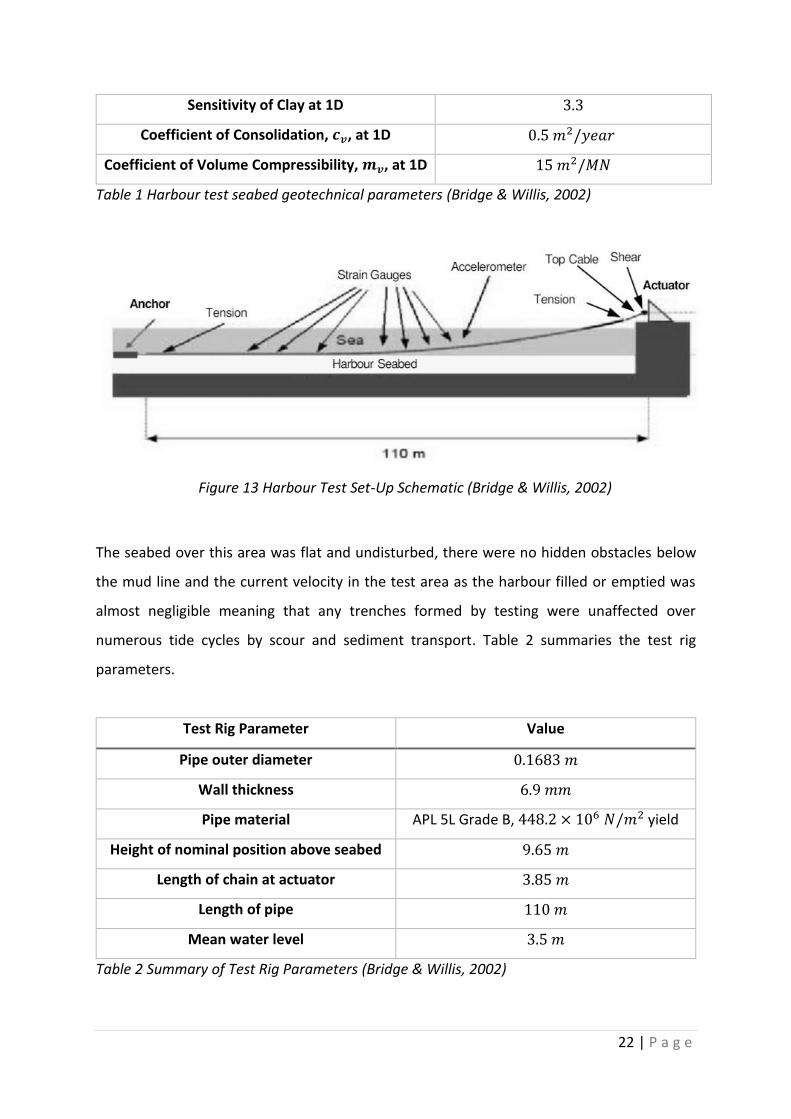
In order for the model to provide reliable results an appropriate value of the installation angle

𝜃 is required. Bridge and Willis (Bridge, et al., 2003) carried out a large scale simulation of

seabed-riser interaction at the touchdown point of deep-water SCRs in Watchet Harbour in

England where the seabed soil is known to have similar properties to a deep-water Gulf of

Mexico seabed. Using the site geotechnical parameters summarised in Table 1 along with

Bridge and Willis’ observations, an estimate of an appropriate input installation angle 𝜃 could

be determined using the MATLAB installation model. The harbour test consisted of a 110 m

long, 0.1683 m diameter welded steel riser suspended from an actuator in the harbour wall

as shown in Figure 13.

Geotechnical Parameter Value

Moisture Content, 𝒘 104.7 %

Bulk Density, 𝝆 1.46 𝑀𝑔/𝑚3

Dry Density, 𝝆𝒅 0.73 𝑀𝑔/𝑚3

Particle Density, 𝝆𝒔 2.68 𝑀𝑔/𝑚3

Liquid Limit, 𝒘𝑳 87.6 %

Plastic Limit, 𝒘𝑷 38.8 %

Plasticity Index, 𝑰𝑷 48.9 %

Average Organic Content 3.2 %

Specific Gravity, 𝑮𝒔 2.68

Undisturbed Shear Strength at 1D 3.5 𝑘𝑃𝑎

Remoulded Shear Strength at 1D 1.7 𝑘𝑃𝑎

22 | P a g e

Sensitivity of Clay at 1D 3.3

Coefficient of Consolidation, 𝒄𝒗, at 1D 0.5 𝑚2/𝑦𝑒𝑎𝑟

Coefficient of Volume Compressibility, 𝒎𝒗, at 1D 15 𝑚2/𝑀𝑁

Table 1 Harbour test seabed geotechnical parameters (Bridge & Willis, 2002)

The seabed over this area was flat and undisturbed, there were no hidden obstacles below

the mud line and the current velocity in the test area as the harbour filled or emptied was

almost negligible meaning that any trenches formed by testing were unaffected over

numerous tide cycles by scour and sediment transport. Table 2 summaries the test rig

parameters.

Test Rig Parameter Value

Pipe outer diameter 0.1683 𝑚

Wall thickness 6.9 𝑚𝑚

Pipe material APL 5L Grade B, 448.2 × 106 𝑁/𝑚2 yield

Height of nominal position above seabed 9.65 𝑚

Length of chain at actuator 3.85 𝑚

Length of pipe 110 𝑚

Mean water level 3.5 𝑚

Table 2 Summary of Test Rig Parameters (Bridge & Willis, 2002)

Figure 13 Harbour Test Set-Up Schematic (Bridge & Willis, 2002)

23 | P a g e

The tests were conducted over a 6 week period on numerous test corridors including an open

trench. It was observed that the open trench was tear-drop in shape with a maximum depth

and width that increased over the 6 week period from 0.5D - 1.2D and 1D - 2.5D respectively

(Bridge, et al., 2003). Therefore it was assumed that installing the riser resulted in a trench

0.5D deep.

The appropriate soil and riser properties were input into the MATLAB model and the riser was

subjected to rotations ranging from 0 radians to 1.5 radians at one end in order to determine

the relationship between maximum trench depth and riser diameter. Figure 14 shows the

results of this computational test. These results show that the relationship between the

vertical displacement and applied installation angle is linear such that

𝑀𝑎𝑥 𝑡𝑟𝑒𝑛𝑐ℎ 𝑑𝑒𝑝𝑡ℎ

𝑅𝑖𝑠𝑒𝑟 𝑑𝑖𝑎𝑚𝑒𝑡𝑒𝑟= 5.42𝜃 Equation 3.20

Thus to achieve a maximum trench depth of 0.5D the installation angle required is 0.09

radians. This is equivalent to 5.16 degrees.

Figure 14 Riser shape when subject to rotation at one end of the riser

24 | P a g e

4 Results and Discussion

4.1 Installation angle

4.1.1 Effect of varying installation angle on trench depth

To verify that the estimate for the installation angle, 𝜃, calculated using the harbour tests is

valid the installation model was run for angles ranging from 0.07 to 0.11 radians and

compared to the post-installation trench field observations carried out by Bridge and Howels

(2007). The model parameters selected represent a generic soil with realistic properties. Table

3 summaries the test parameters used.

Type Parameter Symbol Value

Material

Pipe diameter 𝐷 0.15 𝑚

Wall thickness 𝑡 0.0069 𝑚

Modulus 𝐸 1.93 𝐺𝑃𝑎

Mud-line shear strength 𝑆𝑢𝑜 2 𝑘𝑃𝑎

Shear strength gradient 𝑆𝑔 5 𝑘𝑃𝑎/𝑚

Initial stiffness 𝑘0 1200

Bounding Loop

Power law coefficient 𝑎 6.8

Power law exponent 𝑏 1.2

Maximum uplift load 𝜔 0.65

Uplift load limit 𝜙 0.2

Breakout 𝜓 1.2

Degrading

Re-penetration 𝛼 0.7

Re-penetration 𝛽 0.25

Degrading rate 𝜇 0.01

Degrading rate 𝜖 0.45

Initial load drop Ω 0.35

Interaction

Number of nodes 𝑛 201 (0.5 𝑚)

Maximum iteration - 100

Tolerance 𝜂 0.00001

Installation Axial tension 𝑇 100 𝑘𝑁

25 | P a g e

Installation angle 𝜃 𝑣𝑎𝑟𝑖𝑎𝑏𝑙𝑒

Penetration rate 𝑣 0.05 𝑚𝑚/𝑠𝑒𝑐

Table 3 Model Test Parameters

The tests were carried out on a 100 m long steel riser to which the installation process was

run from 𝑥2 = 80 m to 𝑥1 = 10 m. The main reason for beginning and ending the simulations

away from the very ends of the riser was to prevent the boundary conditions enforced at

these points affecting the results. Additionally by starting the simulation at 𝑥2 = 80 m the

visualization of the effect of the rotation beyond this point was possible.

Figure 15 shows the effect that varying the installation angle has on the trench profile. It

demonstrates that the maximum trench depth increases linearly with installation angle. This

relationship is as expected because as the angle is increased, the riser is forcibly pushed

further into the seabed. The ranges of trench depths observed in the catenary and buried

zone by Bridge and Howells (2007) on SCRs in the Gulf of Mexico and off the coast of Brazil

were between 2.5D - 5D deep. As the range of depths predicted by the model is similar to the

range of those observed in the field it can be concluded that 0.09 radians is a sensible value

of 𝜃 to use in order to accurately model the installation process.

Figure 15 Normalised trench depth for a range of installation angles

26 | P a g e

4.1.2 Effect of varying installation angle on moment envelope

Figure 16 shows the moment envelope along the riser during installation for a range of

installation angles. Overall the maximum hogging and sagging moments are linearly

proportional to the installation angle applied. This is because a larger rotation induces greater

curvatures along the SCR and hence greater bending moments. Note also that the hogging

moments are smaller than the sagging ones as during installation the curvatures experienced

by the riser in the hogging sense are much smaller than those in the sagging sense.

Furthermore the central part of the graph indicates a constant moment envelope between

the locations on the riser where installation process was run. This suggests that the

application of the rotation at each node causes the large maximum sagging and hogging

moments in the riser. Therefore when choosing between the J-lay or S-lay installation

methods it is important to select the one that keeps the installation angle as shallow as

possible to minimise the moment envelope.

Figure 16 Moment envelope for a range of installation angles

27 | P a g e

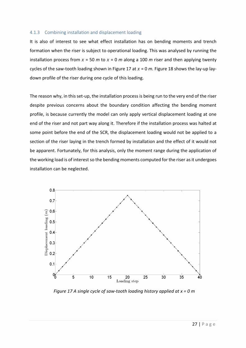
4.1.3 Combining installation and displacement loading

It is also of interest to see what effect installation has on bending moments and trench

formation when the riser is subject to operational loading. This was analysed by running the

installation process from 𝑥 = 50 m to 𝑥 = 0 m along a 100 m riser and then applying twenty

cycles of the saw-tooth loading shown in Figure 17 at 𝑥 = 0 m. Figure 18 shows the lay-up lay-

down profile of the riser during one cycle of this loading.

The reason why, in this set-up, the installation process is being run to the very end of the riser

despite previous concerns about the boundary condition affecting the bending moment

profile, is because currently the model can only apply vertical displacement loading at one

end of the riser and not part way along it. Therefore if the installation process was halted at

some point before the end of the SCR, the displacement loading would not be applied to a

section of the riser laying in the trench formed by installation and the effect of it would not

be apparent. Fortunately, for this analysis, only the moment range during the application of

the working load is of interest so the bending moments computed for the riser as it undergoes

installation can be neglected.

Figure 17 A single cycle of saw-tooth loading history applied at x = 0 m

28 | P a g e

Figure 19 shows the final trench profiles for different combinations of installation and

operational loading. What can be seen from the figure is the large impact that including

installation has on final trench profile after the riser has undergone 20 cycles of the saw-tooth

loading. The maximum trench depth is approximately 6 times greater when installation is

Figure 18 Lay-up and lay-down profile of riser for displacement loading history

Figure 19 Normalised trench depth for various combinations of installation and operational loading

29 | P a g e

taken into consideration and the change in trench depth profile as a result of the loading is

much smaller. This is as expected because during the installation process a deep initial trench

is created and the soil resistance at this depth is greater than that at the surface of the seabed.

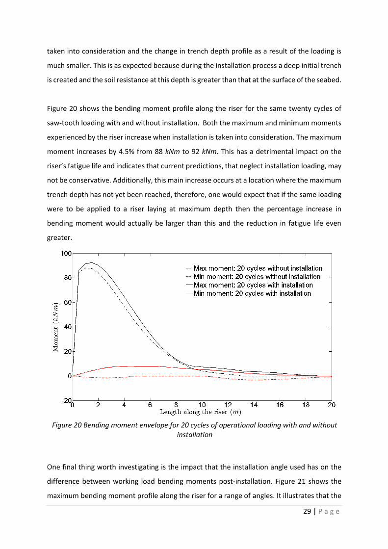
Figure 20 shows the bending moment profile along the riser for the same twenty cycles of

saw-tooth loading with and without installation. Both the maximum and minimum moments

experienced by the riser increase when installation is taken into consideration. The maximum

moment increases by 4.5% from 88 kNm to 92 kNm. This has a detrimental impact on the

riser’s fatigue life and indicates that current predictions, that neglect installation loading, may

not be conservative. Additionally, this main increase occurs at a location where the maximum

trench depth has not yet been reached, therefore, one would expect that if the same loading

were to be applied to a riser laying at maximum depth then the percentage increase in

bending moment would actually be larger than this and the reduction in fatigue life even

greater.

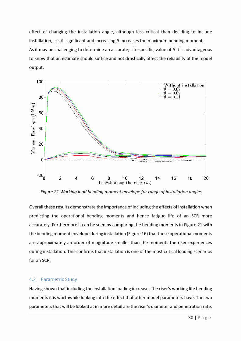
One final thing worth investigating is the impact that the installation angle used has on the

difference between working load bending moments post-installation. Figure 21 shows the

maximum bending moment profile along the riser for a range of angles. It illustrates that the

Figure 20 Bending moment envelope for 20 cycles of operational loading with and without installation

30 | P a g e

effect of changing the installation angle, although less critical than deciding to include

installation, is still significant and increasing 𝜃 increases the maximum bending moment.

As it may be challenging to determine an accurate, site specific, value of 𝜃 it is advantageous

to know that an estimate should suffice and not drastically affect the reliability of the model

output.

Overall these results demonstrate the importance of including the effects of installation when

predicting the operational bending moments and hence fatigue life of an SCR more

accurately. Furthermore it can be seen by comparing the bending moments in Figure 21 with

the bending moment envelope during installation (Figure 16) that these operational moments

are approximately an order of magnitude smaller than the moments the riser experiences

during installation. This confirms that installation is one of the most critical loading scenarios

for an SCR.

4.2 Parametric Study

Having shown that including the installation loading increases the riser’s working life bending

moments it is worthwhile looking into the effect that other model parameters have. The two

parameters that will be looked at in more detail are the riser’s diameter and penetration rate.

Figure 21 Working load bending moment envelope for range of installation angles

31 | P a g e

The same basic model parameters for a generic soil will be used in this analysis as outlined in

Table 3 §4.1.1.

4.2.1 Effect of varying riser diameter

4.2.1.1 Trench Depth

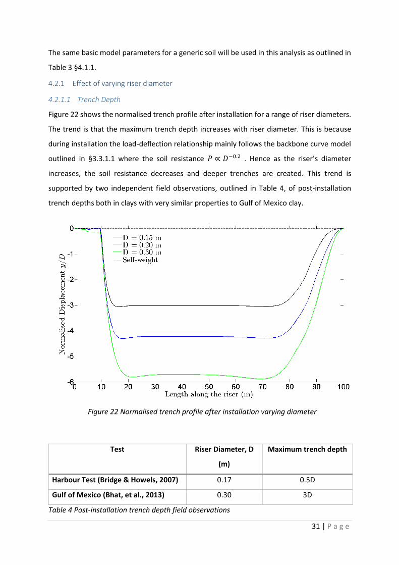
Figure 22 shows the normalised trench profile after installation for a range of riser diameters.

The trend is that the maximum trench depth increases with riser diameter. This is because

during installation the load-deflection relationship mainly follows the backbone curve model

outlined in §3.3.1.1 where the soil resistance 𝑃 ∝ 𝐷−0.2 . Hence as the riser’s diameter

increases, the soil resistance decreases and deeper trenches are created. This trend is

supported by two independent field observations, outlined in Table 4, of post-installation

trench depths both in clays with very similar properties to Gulf of Mexico clay.

Test Riser Diameter, D

(m)

Maximum trench depth

Harbour Test (Bridge & Howels, 2007) 0.17 0.5D

Gulf of Mexico (Bhat, et al., 2013) 0.30 3D

Table 4 Post-installation trench depth field observations

Figure 22 Normalised trench profile after installation varying diameter

32 | P a g e

The observations summarised in Table 4 can also be compared to the 0.15 m and 0.30 m riser

model results. Overall the model predicted deeper trenches than those observed. For

example the observed trench depth for the 0.15 m riser was 0.5D however the model

predicted a trench 3D deep. The reason for this large discrepancy is that the harbour test clay

and the Gulf of Mexico clay have a higher value of undrained shear strength at the seabed

𝑆𝑢𝑜 than that used in the model (approximately 4 𝑘𝑃𝑎 in comparison with 2 𝑘𝑃𝑎). Thus the

model provided less resistance against trench formation and deeper trenches were predicted.

Finally, Figure 22 also shows that as the riser diameter increases, the length of the riser from

the last applied point of rotation (𝑥 = 0 m) to the location at which the maximum trench depth

is reached increases. For example, when 𝐷 = 0.15 m the maximum trench depth is reached at

approximately 𝑥 = 15 m but when 𝐷 = 0.30 m this occurs at 𝑥 = 20 m. This can be explained

because the riser’s bending stiffness increases with diameter and so larger risers will resist

the applied installation more resulting in the maximum trench depth occurring further from

the applied rotation. Figure 23 supports this explanation by illustrating the effect that varying

the bending stiffness of the riser, while applying a rotation of 0.09 radians at 𝑥 = 0 m has on

the maximum trench depth and its location.

Figure 23 Trench profile for a range of bending stiffness'

33 | P a g e

4.2.1.2 Moment Range

Figure 24 shows the moment envelope experienced during installation by risers with

diameters ranging from 0.15 m to 0.3 m. As the diameter increases, so does the minimum and

maximum bending moments. The reason for this non-linear relationship is that as the

installation angle is increased and deeper trenches are formed, as a result of the linearly

increasing shear strength profile, the soil resistance increases resulting in larger bending

moments. It is therefore recommended that the riser diameter is kept to a minimum in order

to reduce the bending moments experienced by the riser during installation, prevent yielding

of the material and prevent the formation of residual stresses.

4.2.2 Effect of varying penetration rate

4.2.2.1 Model Calibration

Apart from installation another thing lacking in the seafloor-riser interaction model

developed by Aubeny and Biscontin is that it cannot directly take account of the penetration

rate of the riser into the soil because the equations it is based on are independent of time. In

order to try and take account of this indirectly, soil model parameters were calibrated so that

the model output for a specific loading history matched, to as great an extent as possible, two

large-scale physical model tests carried out the by the Norwegian Geotechnical Institute (NGI)

in collaboration with Langford & Aubeny, (2008).

Figure 24 Moment envelope for a range of riser diameter's

34 | P a g e

These two single stage cyclic tests aimed to investigate the effect of penetration rate on

seafloor-riser interaction in the touchdown zone. They were carried out on model pipes of

length 1300 𝑚𝑚 and diameter 174 𝑚𝑚, on re-constituted high plastic marine clay with a soil

profile of 2 𝑘𝑃𝑎 at the seabed and strength gradient of 13 𝑘𝑃𝑎/𝑚. The first test was run at a

penetration rate of 0.05 𝑚𝑚/𝑠 and the second test at the faster rate of 0.5 𝑚𝑚/𝑠. During

each cycle the pipe was penetrated to a constant level of soil resistance: about 9.5 𝑘𝑃𝑎 for

Test 1 and 11 𝑘𝑃𝑎 in Test 2, before being lifted to the point of full soil-pipe separation in order

to obtain a complete picture of the suction plateau. There were three model parameters that

were of interest when calibrating the model with these tests: 𝜔, 𝜙 and 𝜓.

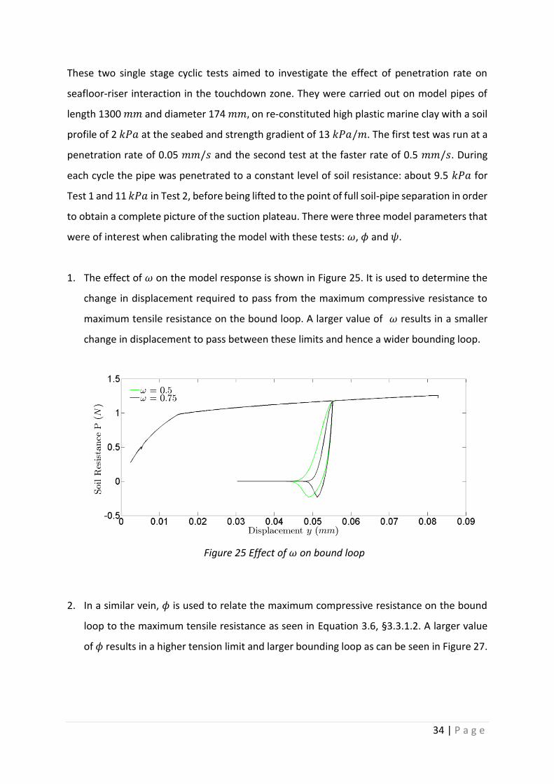
1. The effect of 𝜔 on the model response is shown in Figure 25. It is used to determine the

change in displacement required to pass from the maximum compressive resistance to

maximum tensile resistance on the bound loop. A larger value of 𝜔 results in a smaller

change in displacement to pass between these limits and hence a wider bounding loop.

2. In a similar vein, 𝜙 is used to relate the maximum compressive resistance on the bound

loop to the maximum tensile resistance as seen in Equation 3.6, §3.3.1.2. A larger value

of 𝜙 results in a higher tension limit and larger bounding loop as can be seen in Figure 27.

Figure 25 Effect of 𝜔 on bound loop

35 | P a g e

3. Figure 26 shows the effect of the parameter 𝜓 on the model response. 𝜓 is used to

determine the point where the pipe becomes completely detached from the seabed and

therefore controls how the uplift force decays as seen in Equation 3.6, §3.3.1.2. A larger

value of 𝜓 results in a later detachment of the riser from the seabed and therefore a wider

bounding loop.

Figure 28 and Figure 29 show the large-scale model testing load-displacement curves for the

two NGI large scale tests compared with the model output for penetration rates of

0.05 𝑚𝑚/𝑠 and 0.5 𝑚𝑚/𝑠 respectively. Table 5 summaries the different values of the

degrading parameters just described to calibrate the model to the large-scale test results.

Figure 27 Effect of 𝜙 on bound loop

Figure 26 Effect of 𝜓 on bound loop

36 | P a g e

Figure 28 Test 1 penetration rate v = 0.05mm/sec

Figure 29 Test 4 penetration rate v = 0.5 mm/sec

37 | P a g e

Model Parameter Test 1

v = 0.05mm/s

Test 4

v = 0.5mm/s

𝝓 0.20 0.30

𝝍 1.20 2.00

𝝎 0.65 0.70

Table 5 Summary of affect model parameters for differing penetration rates

Overall, in particular for the first few cycles, the model and large scale tests produce fairly

similar results. However as the number of cycle’s increases, the model fails to capture the

behavior of the soil when subject to tensile loading and neither does the backbone curve

model fit the large scale test data well. Despite these inadequacies, the model parameters

determined to represent the two different penetration rates should be sufficient to

qualitatively compare the effect of penetration rate on installation trench depth and moment

envelope.

4.2.2.2 Effect of penetration rate on the shear strength of clay

There are two main mechanisms which affect the strength and hence response of a clay as a

result of the penetration rate. Firstly the closer the conditions are to fully drained during

penetration, the higher the value of soil resistance because if the penetration is sufficiently

low that the soil ahead of the penetrating object has time to consolidate, then larger shear

strength and stiffness’ are developed than would have done under undrained conditions.

Secondly, in soils with high clay content in fully undrained conditions, the greater the

penetration rate, the larger the undrained shear strength 𝑆𝑢𝑜. (Kim, et al., 2008).

Consequently one would expect that increasing the penetration rate would result in greater

soil resistance and bending moments but shallower trenches. Similarly, the degrading

parameter 𝜔 would increase because the change in displacement required to pass from

maximum compressive to tensile resistance on the bound loop would reduce. One would also

expect a larger tension limit and a greater displacement required for complete detachment

of the riser of the soil leading to an increase in the values of 𝜙 and 𝜓. The values in Table 5

38 | P a g e

support this theory as the parameters calibrated for Test 2 that had the faster penetration

rate are larger than those for Test 1.

4.2.2.3 Trench Depth

Figure 30 shows that increasing the penetration rate during installation reduces the trench

depth which agrees with the theoretical prediction. Moreover it is interesting that increasing

the penetration rate by a factor of ten causes only a 10% reduction in trench depth. Therefore,

it can be concluded that, comparatively, the penetration rate does not have as big an impact

on the final installation trench depth as both installation angle and riser diameter. Finally

Figure 30 suggests that increasing the penetration rate results in a more uneven trench

profile. However it is likely that this is not a function of the penetration rate but of the fineness

of the mesh used for the finite difference analysis. The nodal spacing used for all tests

throughout this report is 0.5 m which is quite large. The reason for not using a finer mesh is

due to the time that the computation analysis would have taken. Therefore, if a finer mesh

were used then one would expect the trench profile for the higher penetration rate to be

more uniform.

Figure 30 Normalised trench depth when varying penetration rate

39 | P a g e

4.2.2.4 Moment Range

Figure 31 shows that the moment envelopes experienced by the riser for the two different

penetration rates are almost identical. This is unsurprising because the bending stiffness’ of

both the risers were identical as was the installation angle and therefore the curvatures

experienced would have been very similar. Again, the probable reason for the unevenness of

the bending moment profile is due to the large nodal spacing along the SCR.

4.3 Design Recommendations

Using the research carried out in this report a number of design recommendations can be

made. Firstly results have shown that is important to minimise the installation angle to keep

the bending moments during installation and post-installation as small as possible.

Additionally, risers with smaller diameters reduce the post-installation trench depth and

bending moments and hence increase the fatigue life of the riser. However, when choosing

the riser diameter size it is important to make sure that it is not too small so that the flow rate

of the oil through the pipe will not exceed a sensible limit. Finally any time that an oil rig

spends not in operation is very costly so it is advantageous that a high laying rate has a positive

effect on the fatigue life of the SCR.

Figure 31 Moment envelope along the riser for when varying penetration rate

40 | P a g e

4.4 Critical Evaluation of the Model

Advantages

The seafloor-interaction model can account for all phases of interaction including non-linear

soil behaviour, soil suction and breakaway, soil yielding, and degradation under cyclic loading.

It is very versatile as any combination of imposed displacements, tension and moments can

be applied and the resultant trench formation and bending moments can be predicted. This

allows for both the modelling of general loading during the working life of the riser as well as

facilitating the installation process. Including the installation process in the program allows

for a more realistic prediction of trench depth and bending moments during the life of a SCR

and highlights the critical nature of the loading it is subject to during installation. Finally the

model has been designed with the view of creating a package that is easily accessible to

designers and can be run on a personal computer. It allows for the manual input of a large of

riser and soil properties to enable the output to be tailored to specific sites and scenarios.

Disadvantages

Determining the backbone curve and bounding loop parameters used in the model require

special laboratory tests involving instrumented pipes penetrating into a clay-filled test basin.

Measurements collected during initial penetration are used to determine the two backbone

parameters 𝑎 and 𝑏 and measurement collected during an unloading cycle can be used to

determine the bounding loop parameters 𝑘0, 𝜔, 𝜙 and 𝜓. Also, in order to achieve better

results a fine mesh with a large number of nodes would be required but, due to the long

length of the riser, and the time required to iteratively solve the ordinary differential equation

at each node for each time step, the time to run the code is too long to be viable. This reduces

the model’s value as a convenient design tool.

Future Considerations

Currently the model allows for the computation of the moments along the riser however it

would be beneficial if the model could use these results to compute an estimated fatigue life

of the riser. Furthermore, the incorporation of time into the model to enable the analysis of

the effect of consolidation would make it even more realistic.

41 | P a g e

5 Conclusion

In conclusion this report has detailed a way to model the installation of SCRs in conjunction

with the non-linear, degrading, seafloor-riser interaction MATLAB model developed by

Aubeny and Biscontin (2009). It requires the manual input of the installation angle 𝜃, and the

two points along the SCR between which the installation process will be run. Observations

from the harbour test carried out by Bridge and Willis (2002) allowed a realistic value of 𝜃 =

0.09 radians to be estimated. One limitation of the installation model is that in order to avoid

the boundary conditions imposed at each end of the riser affecting the bending moment

profile, it must be run sufficiently far away from the ends of the riser. This makes interfacing

installation with future loading on the riser to calculate its fatigue life challenging.

It has been demonstrated that increasing the installation angle used will increase the post-

installation trench depth and moment envelopes of the riser both during installation. Also,

when installation was taken into consideration, the additional trench formation due to

operational loading was greatly reduced and the working load moments were increased. This

informs the recommendation that this angle is kept to a minimum to reduce these moments.

Finally, a parametric study looking at the effect of the riser’s diameter and penetration rate

on trench depth and bending moments identified that increasing the riser’s diameter had a

detrimental effect on its fatigue life but increasing the penetration rate served to reduce the

maximum moments experienced by it. Therefore it is sensible to try and keep the riser’s

diameter to a minimum.

Overall, installation has been shown to be one of the most critical loading scenarios during

the life of a SCR and the development of the MATLAB model to simulate this has enabled

more realistic bending moment and trench depth predictions which will allow for improved

fatigue life estimates.

42 | P a g e

6 References

2H Offshore Engineering Ltd., 2006. Installation of Risers in Deep Waters. Kuala Lumpur,

PetroMin Deepwater and Subsea Technology Conference and Exhibition.

Aubeny, C. & Biscontin, G., 2006. Seafloor Interaction with Steel Catenary Risers, Texas A&M

University: Offshore Technology Reserach Center Report.

Aubeny, C. & Biscontin, G., 2009. Seafloor-Riser Interaction Model. International Journal of

Geomechanics, pp. 133-141.

Aubeny, Shi & Murff, 2005. Collapse load for cylinder embedded in trench in cohesive soil.

Int. J. Geomech, pp. 320-325.

Bhat, S., Jain, S., Randolph , M. & Mekha, B., 2013. Modeling the touchdown zone trench and

its impact on SCR fatigue life. s.l., OTC 2013.

Bridge, C., 2005. Effects of Seabed Interaction on Steel Catenary Risers, s.l.: PhD Thesis,

University of Surrey.

Bridge, C. et al., 2003. Full scale model tests of a steel catenary riser, s.l.: 2H Offshore

Engineering Ltd.

Bridge, C. & Howels, H., 2007. Observations and modeling of steel catenary riser trenches.

Lisbon, ISOPE-2007-468, pp. 803-813.

Bridge, C., Laver, K., Clukey, E. & Evans, T., 2004. Steel catenary riser touchdown point vertical

interaction model. Houston, s.n.

Bridge, C. & Willis, N., 2002. Steel Catenary Risers - Resuilts and Conclusions from Large Scale

Simulations of Seabed Interaction. s.l., 2hoffshore.com.

Callegari & Lenci, 2005. Simple analytical models for the J-lay problem. Acta Mechanica, Issue

178, pp. 23-39.

Clukey, E., Ghosh, R., Mokarala, P. & Dixon, M., 2007. Steel Catenary Riser (SCR) design issues

at touch down area. Lisbon, Proceedings of the Seventeenth International Offshore and Polar

Engineering Conference.

Clukey, E., Houstermans, L. & Dyvik , R., 2005. Model tests to simulate riser-soil interaction

effects in touchdown point region. Perth, Australia, International Symposium on Frontiers in

Offshore Geotechnics.

Dunlap, W. A., Bhojanala, R. P. & Morris, D. V., 1990. Burial of Vertically loaded Offshore

Pipelines in Weak Sediments. Houston, Texas, s.n., pp. 263-270.

43 | P a g e

Giertsen, E., Verley, R. & Schroder, K., 2004. CARISIMA a catenary riser/soil interaction model

for global riser analysis. Vancouver, Proceedings of the International Conference on Offshore

Mechanics and Arctic Engineering.

Hale, J., Morris , D., Dunlap, W. & Yen , T., 1992. Modeling pipeline behavior on clay soils

during storms. Houston, TX, 24th Offshore Technology Conference.

Hetenyi, M., 1946. Beams on Elastic Foundation, s.l.: The University of Michigan Press.

Howells, H., 1998. Steel catenary risers for deepwater environments. Houston, s.n., pp. 1-14.

Karunakaran, D., Farnes, K. A. & Giertsen, E., 2004. Analysis guidelines and application of a

riser-soil interaction model including trench effects. Vancouver, Canada, Proceedings of the

International Conference on Offshore Mechanis and Arctic Engineering.

Kim, K., Prezzi, M., Salgado, R. & Lee, W., 2008. Effect of Penetration Rate on Cone Penetration

Resistance in Saturated Clayey Soils. Journal of Geotechnical and Geoenvironmental

Engineering, pp. 1142-1153.

Mekha, B. B., 2001. New frontiers in the design of steel catenary risers for floating production

systems. Journal of Offshore Mechanics and Artic Engineering, pp. 123, 153-158.

Morris, D., Webb, R. & Dunlap, W., 1988. Self-burial of laterally loaded offshore pipelines.

Houston, Texas, 20th Annual Offshore Technology Conference.

Nakhaee, A. & Zhang, J., 2008. Effects of the interaction with the seafloor on the fatigue life

of a SCR. Vancouver, International Offshore and Polar Engineering Conference.

Pesce, C., Aranha, J. & Martins, C., 1998. The soil rigidity effect in the touchdown boundary

layer of a catenary riser: static problem. Montreal, Canada, Proceedings of the Eighth

International Society of Offshore and Polar Engineers.

Pulici, Trifon & Dumitrescu, 2003. Deep Water Sealines Installation by Using the J-lay Method

- The Blue Stream Experience. Honolulu, Thirteenth International Offshore and Polar

Engineering Conference.

Yen, B. C., Allem, R. L. & Shatto, H. H., 1975. Geotechnical Input for Deep-water Pipelines.

University of Delaware, ASCE, pp. 504-522.

You, J. H., 2012. Numerical modeling of seafloor interaction with steel catenary risers, Texas:

Texas A & M University.

44 | P a g e

7 Appendices

7.1 Appendix 1: Risk assessment

When filling out the risk assessment form at the beginning of the year the only hazards

identified related to this project were to do with computer use. This has proved to be true as

the whole project has been solely computer based. In order to mitigate some of the risks good

posture and ergonomics was used at all times and regular breaks were taken to prevent eye

strain and stiff muscles.