modelling pipeflow contributions to stream runoff
TRANSCRIPT

HYDROLOGICAL PROCESSES, VOL. 2, 1-17 (1988)
MODELLING PIPEFLOW CONTRIBUTIONS TO STREAM RUNOFF
J. A. A. JONES University College of Wales, Aberystwyth, Wales
ABSTRACT Runoff from natural soil pipes has been shown to be a significant contributor to stream discharge in parts of upland Wales. Attempts have been made to model pipeflow contributions using both theoretical and empirical approaches, but little progress has yet been made towards producing generally applicable models of complete pipeflow systems.
The paper identifies some of the problems of devising general models with reference t o data from the Maesnant Experimental Catchment. The data suggest that in-pipe travel times are more important here than inferred elsewhere, and that neither simple hydraulic models nor kinematic wave theory can adequately explain the patterns of response. In particular, stormflow tends to begin first at the network outfall and even peak discharge often occurs at the outfalls before the headward zones.
KEY WORDS Pipeflow Runoff modelling Soil pipes
INTRODUCTION
Evidence from a number of recent field monitoring programmes has shown that pipeflow can be a substantial contributor to storm quickflow in a variety of locations in the U.K. (Jones, 1979; Gilman and Newson, 1980; McCaig, 1983; Wilson and Smart 1984; Jones and Crane, 1984; Jones, 1987). Each of these field teams has consequently recognized the need to model pipeflow contributions with the ultimate aim of incorporating a pipeflow component in general models of the rainfall-runoff process. Current research on the impact of acid rainfall and in solute movement on hillslopes is also demanding more realistic models of drainage pathways above and beyond the limits of the stream channel network (Welsh Water Authority, 1986).
The central question explored in this paper is the degree to which empirical location-specific models of pipeflow may be replaceable by more theoretically based models that are more generally applicable.
APPROACHES TO MODELLING
The overall problem of modelling pipeflow contributions can be broken down into four components. The first and possibly the most intractable component is the source or sources of pipeflow, whether these be via rising phreatic water, rainfall infiltrating vertically through the soil matrix, or overland flow captured by blow-holes and surface macropores, and the spatial distribution of these sources. The second concerns the properties of the pipe channels and the rate of transmission along the pipes. The third component is the structure and continuity of the pipe network, which together with the second component needs to be understood for any realistic simulation of flow routing. The final component is the position of the pipe outfalls relative to open channels. Of all these components, the question of rates of transmission along the pipes should be the most readily accessible from established hydraulic theory, and appears to offer a useful starting point for more theoretically based models.
To date, three types of approach have been taken to predicting pipeflow contributions. Firstly, very
0885-6087/88/010001-18$09.00 0 1988 by John Wiley & Sons, Ltd.
Received 23 March 1987

2 J . A. A. JONES
empirical indirect approaches have been taken by McCaig (1983) and Wilson and Smart (1984) simply to estimate the relative importance of pipeflow in the absence of direct measurements. McCaig (1983) used measurements of dissolved solids concentrations in pipeflow and in streamflow and applied a simple mixing model to infer the proportion of storm quickflow generated from pipe sources. He adduced evidence to suggest that dissolved solids concentrations in pipeflow are independent of discharge to support this approach, although more recent evidence from the Maesnant basin contradicts this (Hyett, personal communication). Wilson and Smart (1984) estimated pipeflow using average pipe capacities calculated from artificial pumping experiments and the distribution of pipes estimated by air photo-interpretation.
Secondly, direct measurements of pipeflow hydrographs have been used to establish statistical models and to infer causal factors by Gilman and Newson (1980) and Jones and Crane (1984). Gilman and Newson (1980) first took a hydrograph synthesis approach in which a set of up to four parameters was fitted by numerical optimization. The relative importance of the parameters was used to infer the sources and mechanisms of flow generation. Jones and Crane (1984) and Jones (1986; 1987) used a continuous record of pipeflow contributions and applied stepwise multiple regression analyses to establish causal factors and predictive models.
Thirdly, more theoretical approaches have been taken by Gilman and Newson (1980) and McCaig (1983) who were specifically concerned with the problem of modelling the transmission of water through the pipe system. These authors have used hydraulic theory to predict travel times within the network, McCaig relying on a model developed directly from the Chezy formula and Gilman and Newson taking the more sophisticated approach of kinematic wave theory.
Pipeflow travel times derived f rom the Chezy formula McCaig (1983) derived a simple model for pipeflow contributions on rectilinear slopes using the Chezy
equation and making a number of simplifying assumptions: that (i) in the absence of flow convergence, discharge increases linearly with distance downslope, x ,
Q = k’x (1)
(ii) pipes are discharging constantly at half full, and (iii) the roughness coefficient, a, is inversely proportional to pipe radius, r , thus n = l / k r . On this basis McCaig deduced a power law relationship between pipe radius and distance downslope,
k ’ x ’/I
r = (5) = k”’x”’
By incorporating field data on pipe size, spacing and velocities, McCaig was able to estimate the constants, k . He concluded that 90 per cent of the travel time for pipeflow occurs prior to entry into recognizable pipes, mainly in passing through small soil pores, and that it is slow drainage through these feeder pores that causes pipeflow recession to be less rapid than recession from other quickflow sources.
Beguiling though this simple formulation is, initial comparison with observations in the Maesnant experimental basin (Figure 1) suggests that it is too oversimplified to be generally applicable. Even on a hillslope which appears to be fundamentally rectilinear on the 1:25,000 map, the pipe network itself can generate both surface and subsurface convergence, as illustrated by Jones’s (1986) reservations on the a/s index. Moreover, the continuous rainfall and pipeflow data for Maesnant suggest that lag times at the outfall of the perennial pipe system are accounted for by a much more even split between pre-pipe and inpipe travel times. Taking lag times between peak rainfall intensities and peak pipeflow runoff intensities as an illustration, the mean lag at the head of the perennial pipe network (pipe weir 9 in Figure 1) is just 1.2 h with a further 1.6 h delay occurring in transmission down the 323 m section to the pipe outfall (at site 4 on Figure 1).
We will return to the limitations of this approach after considering the kinematic wave approach.

MODELLING RUNOFF FROM PIPES 3
I STREAM UPPER WE1 , ; /
L
1 f
0 50 100
Metres
;/----/ TREAM LOWER WEIR'
Figure 1. The Maesnant experimental basin and flow monitoring sites
Theoretical kinematic wave velocities Gilman and Newson (1980) used measurements from the Upper Wye catchment taken during an
artificial pumping experiment to calculate an empirical power law relationship between discharge, Q , and the cross-sectional area of flow, A , in a pipe. Differentiating this equation with respect to cross-sectional area gives the.flood wave velocity, c. Thus an equation of the form
Q = kA" (3)
4 J . A. A. JONES
Table I. Relationships between cross-sectional area of flow ( A ) and discharge (Q) in pipes
Discharge:area Correlation Equation including equation coefficient pipe slope, S
or more generally
can be differentiated to give
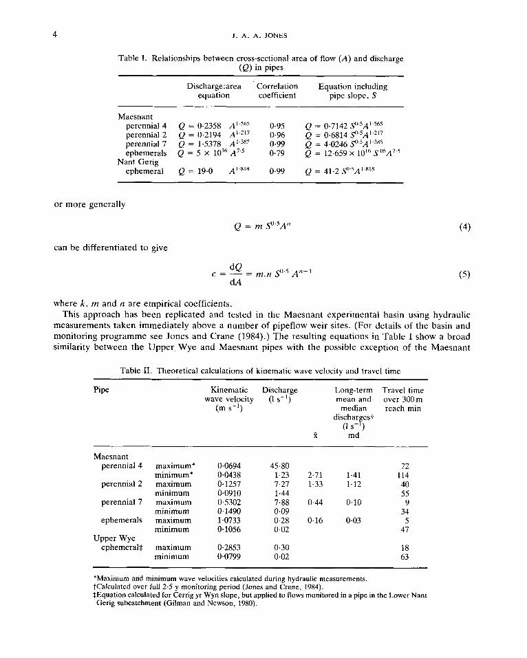
where k , rn and n are empirical coefficients. This approach has been replicated and tested in the Maesnant experimental basin using hydraulic
measurements taken immediately above a number of pipeflow weir sites. (For details of the basin and monitoring programme see Jones and Crane (1984).) The resulting equations in Table I show a broad similarity between the Upper Wye and Maesnant pipes with the possible exception of the Maesnant
Table 11. Theoretical calculations of kinematic wave velocity and travel time
Pipe Kinematic Discharge Long-term Travel time wave velocity (I S - I ) mean and over 300m
(m s - I ) median reach min dischar est F (1 s- 1
% md
Maesnant perennial 4 maximum* 0-0694 45-80 72
minimum* 0.0438 1.23 2.71 1.41 114 perennial 2 maximum 0.1257 7.27 1-33 1.12 40
minimum 0-0910 1.44 55 perennial 7 maximum 0.5302 7.88 0-44 0.10 9
minimum 0.1490 0.09 34 ephemerals maximum 1-0733 0.28 0.16 0.03 5
minimum 0.1056 0.02 47
ephemera13 maximum 0-2853 0-30 18 minimum 0.0799 0.02 63
Upper Wye
*Maximum and minimum wave velocities calculated during hydraulic measurements. fCalculated over full 2.5 y monitoring period (Jones and Crane, 1984). $Equation calculated for Cerrig yr Wyn slope, but applied to flows monitored in a pipe in the Lower Nant Gerig subcatchment (Gilman and Newson, 1980).

MODELLING RUNOFF FROM PIPES 5
ephemeral pipes; however, this latter case should be treated with caution since, in order to obtain a usable sample size, data from more than one pipe were combined.
Using these equations to calculate kinematic wave velocities, nevertheless reveals marked differences between pipes (Table 11). In order to compare travel times, a standard distance of 300 m has been used in Table 11, which is the same as the length of the Lower Nant Gerig pipe used by Gilman and Newson (1980) and roughly equivalent to the separate lengths of the ephemeral and perennial sections of the Maesnant network. In high flows, the ephemeral pipes are particularly efficient water transmitters in both basins, but there is a very marked decrease in wave velocities given an order of magnitude fall in flow. In comparison, transmission through the perennial pipe network is considerably slower for equivalent and even for very much higher discharges. But the contrasts in efficiency between high and low flows are less, with the exception of perennial pipe 7, which is closest to the ephemeral pipes both spatially and in terms of flow patterns (Jones and Crane, 1984; Jones, 1987).
It is possible to estimate relative frequencies for these travel times on Maesnant using the 2.5 years of continuous flow records available for this basin. Mean discharge in the ephemeral pipes was 0.16 1 s-', with a median of 0.025 1 s- ' . This suggests that for 50 per cent of stormflows travel time through the ephemeral network should be less than three-quarters of an hour, and it should be nearer one-quarter of an hour in flows above mean discharge. In perennial pipe 7 the median discharge would sustain a wave travel time of half an hour, whereas in perennial pipe 4 it would be over 1.5 hours.
PATTERNS AND RATES OF TRANSMISSION - THE FIELD EVIDENCE
The pipeflow records for Maesnant have been used to test these predictions, making particular use of response times at the four strategic monitoring levels on the hillslope - the head and foot of the ephemeral pipes and the head and outfall of the perennial pipes (Figure 1).
Do wnslope transmission The field evidence suggests that the pipe network as a whole cannot be seen as a simple system for the
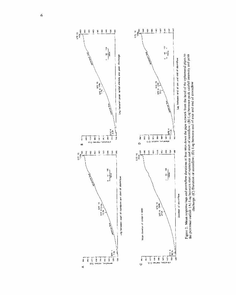
transmission of a kinematic wave down the hillslope in the almost unmodified fashion suggested by Gilman and Newson (1980,84). Storm response tends to begin at the base of the slope and work upwards (Figure 2). Even peak discharge cannot be said to progress simply from upslope to downslope. Peak discharge only progresses smoothly downslope within the well-integrated perennially-flowing section of the network (Figure 2). Even then, progress varies considerably from storm to storm, and the average lag time of 1.5 hours between source and outfall within the perennial system, which appears to be close to the kinematic wave theory prediction, in fact conceals many events in which the pattern is reversed. Predictions based on simple hydraulic theory such as proposed by McCaig (1983) clearly would not work on Maesnant.
The problem is partly due to the fact that the theoretical approaches taken hitherto do not take adequate account of spatially uneven contributions of discharge to the pipe networks. In their simulation analysis Gilman and Newson (1980) explicitly assume that any lateral inflow has the same time distribution as the pipeflow. The problem assumes greater importance when lag times are not merely of the order of 12 minutes (with lateral inflow) or 23 minutes (without) as observed by Gilman and Newson, or less than 15 minutes as deduced by McCaig. Lag times on Maesnant pipes are of the order of hours even in events when a simple downslope transmission of a flood wave appears to be predominant.
Downhill from mid-slope, storm response begins earlier and ends later further downslope. Table I11 shows that storm response begins at monitoring site 4, the outfall alongside the Maesnant stream, on average 5.7 hours after rain begins, whereas the ephemeral section at site 15 takes almost twice as long to respond. Whilst the ephemeral section tends to cease flow 8 hours before the rain ends, the perennial outfall continues to respond for another day after the end of the rainstorm. As a result, the average stormflow event at the outfall lasts for two days compared with just one day at site 15. Taking the ratio of the flow durations in sets of identical storm events (bottom of Table 111) rather than overall averages, the difference is even more marked, with stormflow in the ephemeral section for little over half as long as at
z 580
SITE
9 1
1'5h
500
0 50
10
0
-
met
res
SIT
E
16
1Z.O
h ,r6e
0 ~ 64
0
-620
- 600
g 600-
- 580
- 560
z 5
80-
-540
- - 5
20
W
SITE
4
500
640 -
2 620
-
c
c
0 50
10
0
-
met
res
-0'"
- 600
- 580
- 560
-540
- 520
SITE
16
2
00
h I 66
0
- 640
-620
an d
urat
ion of
ram
fall
= 2
88
h
c 680-
64
0 -
2 620-
- 600
L580
- 560
-540
g 600-
E 580-
6 580-
0
50
1W
-
-2e
-520
0
SITE
4
500
Dur
atio
n of
sto
rmflo
w
640-
520-
E 6W-
E 58
0-
0 -
- 540
-520
- 500
0
50
10
0
-
met
re3
bg
bet
wee
n pe
ak r
ainf
all i
nten
sity
and
pea
k di
scha
rge
600
SITE
15
5
80
56
0
SITE
9
Og
h
0
-620
- 600
640-
520-
E 6W-
- 56
0
E 58
0-
- 540
6 56
0-
- -5
20
54
0-
SITE
4
- 500
- -500
0
50
10
0
-
met
re3
bg
bet
wee
n pe
ak r
alnf
all i
nten
sity
and
pea
k di
scha
rge
SIT
E 1
6
1 @?:660
D
660-
-M
o
- 620
640 -
620-
- 600
600-
- 5
80
- 560
0
50
10
0
- 520
SI
TE 4
500
c E 58
0-
r
-540
g
560-
-
540-
520- 1
1.2h
50
0-
bg
bet
wee
n en
d of
rai
n an
d en
d O
f st
orm
flow
Figu
re 2
. M
ean
resp
onse
lags
and
sto
rmfl
ow d
urat
ions
at f
our s
ites d
own
the
pipe
net
wor
k fr
om t
he h
ead
of t
he e
phem
eral
pip
es to
th
e pe
renn
ial o
utfa
ll: (
A)
Lag
bet
wee
n st
art o
f ra
inst
orm
and
sta
rt o
f st
orm
flow
; (B
) L
ag b
etw
een
peak
rai
nfal
l int
ensi
ty a
nd p
eak
disc
harg
e; (
C) D
urat
ion
of s
torm
flow
; (D
) La
g be
twee
n en
d of
rai
n an
d en
d of
sto
rmfl
ow

M O D E L L I N G R U N O F F F R O M PIPES 7
Table 111. Mean response characteristics a t three points down the pipe network, from ephemeral outfall to perennial outfall (sites 1.5, 9 and 4 respectively). (Time in hours. Standard deviations in brackets. Sample sizes:
45 for sites 4 and 9, 22 for site 15)
Response parameter
Ephemeral outfall Source of perennials Perennial outfall
Duration of
Parameters relative to rainfall: Lag in start time 10-51 (6.18) 8.01 (6-26) Lag in peak -0-99 (11.92) 1.21 (9.89) Lag in time of end -8.25 (16.26) 6-93 (22.06) Lag in time of projected -8.10 (16.05) 22.01 (31.90) end of flow Parameters relative to next monitoring point upslope: Lag in start
Lag in time
Lag in time of end of stormflow
b) projected
Parameters relative to central monitoring site: Ratio of
stormflow Ratio of
areas
stormflow 25.50 (22.59) 40.05 (28.09)
of stormflow -3.12 (4.69)
of peakflow 0.06 (2.14)
a) actual end 16.56 (17.01)
end 32.73 (32.04)
duration of 0.59 (0.36) 1.0
contributing 0.08 (0.04) 1.0
58.85 (30.25)
5-66 (5.74) 2-77 (9.81)
23-37 (15.86)
50.06 (33.72)
-2.36 (5.62)
1 6 6 (4.20)
16.45 (19.03)
47.76 (31.93)
2.04 (1.58)
4.68 (3.63)
the source of the perennial section and stormflow at the outfall being twice as long as that as the source of the perennial section.
The implication would seem to be that increasing soil water content, higher saturation levels and centralization of throughflow networks on the lower sites makes them respond more readily and for longer periods. This is in agreement with the view expressed by McCaig (1983) that the saturation excess model of runoff generation is applicable to pipeflow. However, McCaig proceeded to outline a model of pipeflow generation and contribution based on downslope travel time within the pipe network using the Chezy formula without considering spatial variations in the relationships between pipe beds and the phreatic surface. On Maesnant, there is a marked discontinuity in the hydrological properties of the solum between the upslope ephemeral pipes and the perennial pipes downslope. The ephemeral pipes run near the base of the 150mm thick organic layer in a shallow soil (<400mm) on permeable shattered bedrock and a steeper slope (W), whilst the perennial pipes flow under 0.5-1.0m of peat above an impermeable soliflucted till and on a gentler slope (6") which has a perennial phreatic level within the solum. Whilst there is a noticeable difference in response times between the top and bottom of the perennial section, the change at mid-slope is more marked. Table I11 hides this mid-slope discontinuity somewhat, because although the lags in relative response times are comparable over the two sections of

8 J . A. A . JONES
Table IV. Duration of flows on the upper slope (%)
head of foot of head of ephemeral ephemerals perennial
site 16 14 15 17 9 as % duration of
stormflow at outfall 78 73 43 82 68 - site 4 rainstorm 63 98 58 109 97
network (sites 15 to 9 and 9 to 4), the upper sites are only 64 m apart, whereas the lower two are 323 m apart.
Analysis of response patterns above mid-slope is more difficult since the ephemeral pipes which occupy that part of the slope are less well integrated as a network and more intractable to trace because of their small size (50-100mm or less in diameter) and infrequent flows. Data collected from a site at the uppermost limit of the pipe network on this slope, site 16 on Figure 2, do not fit in very well with the response observed at site 15. This suggests, for example, that during the same rainfall events the average duration of stormflow at the top of the ephemeral network is approximately twice that at the foot (Figure 2). One possible explanation for this could be substantial losses of pipewater by influent seepage, as suggested by Newson and Harrison’s (1978) pumped water experiments in the Upper Wye catchment. A more likely explanation, however, is that the pipewater from site 16 drains down other pipes and bypasses site 15. This latter explanation is supported by measurements from another site at the foot of the ephemeral slope, site 14, which shows an average duration of flow of 26.3 hours, comparable to the 28-0 hours at the top of the slope during the same storms.
It is, in fact, very difficult to relate measurements at the various upslope sites, partly because of the infrequency of flows and therefore small sample sizes and partly it seems because of an inherently wide variety of responses. Table IV illustrates this variety in terms of flow durations.
The variety underlines a fundamental feature of these pipe networks, namely, that the response in adjacent and apparently similar pipes can be very different, and this presents a major difficulty for designing field monitoring schemes and for modelling runoff from pipe systems (Jones, in press). The variety is due to differing sources of pipeflow and differing contributing areas. It means that, although sampling pipe cross-sections may give an approximate indication of gross yields (Jones, 1986), the temporal aspects of pipe response in the basin cannot be calculated simply on the basis of sampling cross-sections, velocities, and the spacing of the pipes as used in McCaig’s (1983) model. Different pipes appear to derive differing proportions of flow from further upslope as opposed to local sources and these proportions vary over time. Travel times to the pipes are likely to be very different when overland flow feeds into blowholes in the pipes compared with saturated or unsaturated throughflow. Moreover efficacy of effluent seepage as a source of pipeflow is a function of the depth of piping as well as size and spacing.
In fact, the size of the tributary pipe network is the best single indicator of hydrological behaviour. Pipes with the swiftest response, longest flow duration, and greatest volumes of stormflow tend to have the largest microtopographic depressions directing overland flow and throughflow towards the master pipe. They also tend to have access to a larger length of ephemeral feeder pipes that creates shorter concentration times (Jones, 1986). Such pipes are also more likely to have beds running below or near to long-term phreatic surfaces.
Hydraulic parameters ,
Hydraulic measurements on the Maesnant pipes confirm many of the observations of Gilman and Newson (1980), but they also offer less support for McCaig’s (1983) model. There is a broad relationship between pipe radius and discharge as McCaig proposed. Indeed, pipe diameter has been found to be a

MODELLING RUNOFF FROM PIPES 9
reasonable substitute for the size of the tributary network in predicting stormflow volumes and contributing areas on Maesnant (Jones, 1986; 1987). However, there is no unique relationship between pipe size ( r ) and distance downslope (x) such as predicted by Equation 2. Reconnaissance along two of the longest known integrated sections of ephemeral and perennial pipes (for 74 m along pipe 16 and 193 m along pipe 4 respectively) indicates (a) some irregularity in the downslope increase in radius involving local reversals in the trend, (b) that the increase is more linear than exponential in both categories of pipe, and (c) that the rate of increase in the two pipes is very different. For the perennial pipe the best fit relationship was:
r = 141.0 + 0 . 3 0 8 ~ (2 = 90.4 per cent) (6)
A power law relationship explained only 61.5 per cent of the variance and the best-fit exponent was 0.052 compared with McCaig’s 0.273.
For the ephemeral pipe the best equation was:
r = 16.2 + 0 . 7 9 1 ~ (2 = 65.0 per cent) (7)
The power law relationship explained only 42.5 per cent of the variance, although the exponent of 0.222 was tolerably close to McCaig’s prediction (Equation 2). In fact, if McCaig’s assumptions are at all reasonable, they should apply in this latter case: along an unbranched ephemeral pipe on a straight slope at the very top of the network. Elsewhere not only do slopes converge towards many pipes, but branches also converge causing irregular increases in discharge. Less commonly they may suffer divergence, anastomosing both laterally and vertically (cf. Wilson and Smart, 1984) or breaking up into distributaries (as above sites 2B and 14 on Maesnant).
Pipes also tend to be very ‘immature’ rough channels. The main reason for this would seem to be that the erosive power of pipeflow tends to be lower in relation to the resistance of soil materials than the erosive power of stream channels. Indeed, flows within soil pipes are more likely to be laminar (or at least have Reynolds’ Numbers, Re, within the range generally regarded as laminar) than flows in stream channels.
All hydraulic measurements taken in the ephemeral pipes on Maesnant have indicated Re <300. Gilman and Newson (1980) calculated values of 58 < Re < 425 for similar shallow ephemeral pipes based on the mean cross-sectional area of pipes in the Wye catchment. Hydraulic measurements in the perennial pipes on Maesnant indicate that out of 26 cases 20 per cent of flows had Reynolds’ Numbers over 1000. These were for high flow situations at sites 4, 9, 5 and 7. These pipes would be likely to show smoother increases in diameters downslope were it not for frequent large boulders within the solum in this area and the occasion advent of a tributary.
Random variations in the resistance of the walls are therefore reflected in variations in the diameter of the pipes and in flow velocities, with pressure flow occurring through restricted sections during some storms. This may even be the cause of a pulsating flow such as that observed by Tanaka, Yasuhara and Marui (1982) in the Hachioji catchment, Japan, and at site 1 on Maesnant (Jones, 1978).
A general result of the irregular shape and size is high roughness. Calculations of Manning’s n values on Maesnant pipes range from 0.06 to 1.15 with an average of 0.33 in the perennial pipes. These are much higher than the values calculated by McCaig (1983) in Yorkshire, which did not exceed 0-15, and nearer to values calculated for overland flow on grass. Gilman and Newson (1980, 83) also concluded that natural pipes behave as extremely rough channels because flow is dominated by channel form rather than skin resistance. They calculated values of Re.f (the product of the Reynold’s number and the Darcy-Weisbach friction coefficient) approaching 2600 for ephemeral pipes, compared with 24 for a smooth channel.
The values of Re. f for Maesnant pipes corroborate the findings of Gilman and Newson. Moreover, they suggest that Re. f values in the perennial pipes can be more than an order of magnitude higher than in the

10 J . A. A . JONES
ephemeral pipes of the Wye, notably at baseflow discharges. At baseflow the largest perennial pipe on Maesnant has Re.f values higher than normally found in overland flow on grass slopes.
It is interesting to see Re. f values in the perennial pipes falling back to within the range of ephemeral pipes at high flows, which suggests that they are hydraulically more efficient in stormflow. At higher flows protruding boulders become less of an obstacle and the perennial pipes are hydraulically more efficient than overland flow on grass slopes, for which Morgali (1970) quotes Re.f values of 500CL14000.
An important hydrological corrollary of this increased efficiency is generally higher velocities of stormflow and reduced travel times within the perennial pipes at high flow levels. Figure 3 shows an overall increase in velocity, V , with discharge, Q, which is particularly clear in the largest perennial pipe (4). The empirical relationship for pipe 4 is:
V = 0.025 Q0.743 (2 = 99.5 per cent, units as Figure 3 ) (8)
which, interestingly, displays an exponent half way between the 0.5 suggested for ephemeral pipeflow by Newson and Harrison's (1978) field experiments and the 1-0 suggested for overland flow. The lower rate of increase in dynamic storage in pipe 4 is also more akin to the overland flow situation and underpins the flashy response (cf. Gilman and Newson, 1980, 97). Other pipes show lesser increases in the rate of transmission with discharge. Data for pipe 7 indicate:
V = 0-481 Q".259 (3 = 90.5 per cent) (9)
The net result is a clear convergence in velocities and dynamic storage which results in very similar values for all pipes at discharges of 101 s-' and above (Figure 3).
The increased velocities at high flows do not, however, result in shorter peak travel times between gauge sites 9 and 4; r = 0.07 for a sample of 52 discharges and travel times. It is clearly not simply a question of transmission of a kinematic wave. In 76 per cent of all storms the average peak travel time is 2.96h (s = 3.77h). But for the remaining one event in four when the outfall peaks first, it does so by an average of 2.77h (s = 1.81). This gives the overall mean peak lag time of the expected sign and magnitude, as already noted (Table 111), but it hides the true nature of events, which owes more to intervening contributions from tributary pipes, overland flow, and the phreatic surface.
Basin-wide patterns under different meteorological states The set of maps in Figures 4 to 6 have been constructed to give a broader, basin-wide perspective of
response patterns, focusing respectively on start lags (Figure 4), peak lags (Figure 5), and end lags (Figure 6) relative to rainfall under differing meteorological conditions. Four typical events have been selected for each parameter to represent two levels of storm severity (light rain and heavy rain) and two levels of antecedent moisture conditions (dry and wet). The maps are presented in the form of a 2 x 2 matrix.
Figure 4 confirms the general tendency for response to begin at the foot of the network. In dry conditions, the ephemeral pipes are slower to start than the perennials. The distributary overflow pipes towards the lower stream weir also respond later in dry conditions, but may be the first to respond in wet conditions when baseflow in the main pipes is already at or above the level needed for overflow into these distributaries (cf . Jones and Crane, 1984).
Figure 5 indicates generally shorter times to peak in wetter antecedent conditions, with some peaks even slightly ahead of rainfall peaks in ephemeral and overflow pipes during wet weather, perhaps indicating flows reaching pipe capacity. There is a general tendency for a longer peak lag at the base of the slopes, which is more exaggerated in dry conditions.
The pattern of end lags in Figure 6 shows that the ephemeral pipes tend to cease flow before the rainfall ends, although they may continue to flow beyond the end of the storm after heavy rain. Perennials, overflows (8 and 2B on Figure 1) and seasonal pipes (6 on Figure 1) all exhibit more persistent storm discharge after heavy rain. However, in the perennial pipes the relative persistence is longer following dry

MODELLING RUNOFF FROM PIPES 11
A Velocity versus discharge on Maesnant pipes
1 .o 10.0
discharge Is-' 100.0
Dynamic storage versus discharge on Maesnant pipes 8.
- - - ephemeral pipe on Nant Gerig (Newson and Harrison)
ephemeral headwater pipe on Maesnant
I
0.1 1 .o 10.0 lo00
discharge Is-'
Figure 3. Velocity (A) and dynamic storage (B) as a function of discharge in pipes on Maesnant. The relationships calculated for an ephemeral pipe on Nant Gerig by Newson and Harrison (1978) are included for comparison
conditions. This may be simply because in wet conditions the next storm arrives before delayed flow is complete.
FACTORS AFFECTING LAG TIMES AT CRITICAL LOCATIONS IN THE PIPE NETWORK
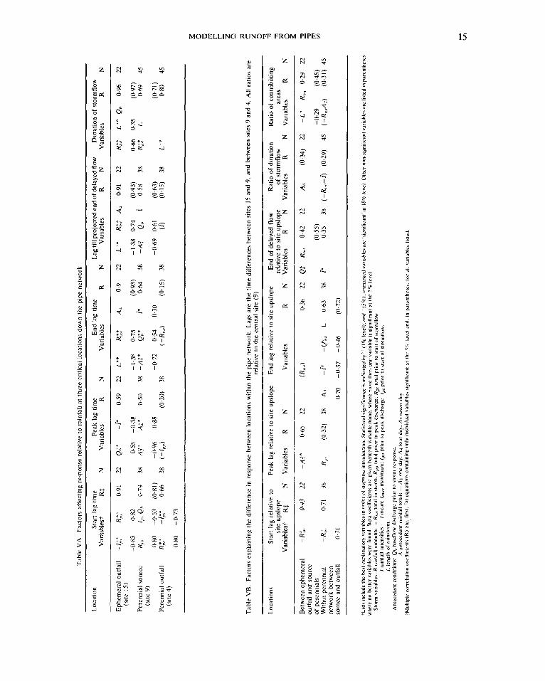
Stepwise multiple regression analyses were used to explore the Maesnant data for factors that might explain the differences in response within the network between sites 15 and 4. The results listed in Table VA show a broad similarity in factors controlling the start of pipe stormflow in both ephemeral and

12 J . A. A. JONES
S N O l l l Q N 0 3 l N 3 0 3 3 3 1 N V AHQ

MODELLING RUNOFF FROM PIPES 13
S N O l l l a N 0 3 l N 3 a 3 3 3 1 N V 13M

14 J . A . A. JONES
\
SNOIlIQN03 lN3Q3331NV 13M SNOIlICINO3 lN3Q3331NV AHQ
Tab
le V
A.
Fact
ors
affe
ctin
g re
spon
se r
elat
ive
to r
ainf
all
at t
hree
crit
ical
loc
atio
ns d
own
the
pipe
net
wor
k
Loca
tion
Star
t la
g tim
e Pe
ak l
ag t
ime
End
lag
time
Lag
till p
roje
cted
end
of d
elay
ed fl
ow
Dur
atio
n of
sto
rmflo
w
RN
V
aria
bles
? R
$ N
V
aria
bles
R
N
Var
iabl
es
R
N V
aria
bles
R
N
V
aria
bles
Ephe
mer
al o
utfa
ll -C
’ R,,’
,’ 0.
91
22
QS’
-i*
0.59
22
L*
* R:
,: A
, 0.
9 22
L”
R:;;
A,
0.91
22
R,
!,,‘
L”
Qh
0.96
22
(s
ite 1
5)
-043
0.
82
0.55
-0
.38
-1.3
8 0.
75
(0.9
3)
-1.3
8 0.
74
(0.9
3)
0.66
0.
35
(0.9
7)
Pere
nnia
l sou
rce
R,,,
-I,,,
Qh
0.79
38
A
;’
A;’
0.
50
38
-A:*
QZ
’ i*
0.64
38
-A
T Q,,
i 0.
58
38
RA;
L 0.
69
45
(site
9)
0.80
-0:
S3
(0.8
1)
-0-9
6 0.
88
-0.7
2 0.
54
0.30
-0
.69
0.61
(0
.63)
(0
.71)
Pe
renn
ial o
utfa
ll R;
>’
-1;:
0.66
38
(-/
,,/,)
(0.2
0)
38
(-R,o
O
(0.1
5)
38
(1)
(0.1
5)
38
L’”
0.80
45
(s
ite 4
) 0.
80
-0.7
3
ia c z 0
?I 7
Tabl
e V
B.
Fact
ors
expl
aini
ng th
e di
ffer
ence
in r
espo
nse
betw
een
loca
tions
with
in t
he p
ipe
netw
ork,
Lag
s ar
e th
e tim
e di
ffer
ence
s bet
wee
n si
tes
15 a
nd 9
, and
bet
wee
n si
tes
9 an
d 4.
All
rat
ios
are
rela
tive
to t
he c
entr
al s
ite (
9)
Loca
tions
St
art
lag
rela
tive
to
Peak
lag
rel
ativ
e to
site
ups
lope
E
nd la
g re
lativ
e to
site
ups
lope
E
nd o
f de
laye
d flo
w
Rat
io o
f du
ratio
n R
atio
of
cont
ribu
ting
7
site
ups
lope
re
lativ
e to
site
ups
lope
of
sto
rmfl
ow
area
s R
N
Var
iabl
es
R N
Var
iabl
es
R
N V
aria
bles
R
N
V
aria
bles
V
aria
bles
t R
$ N
V
aria
bles
R
N
Bet
wee
n ep
hem
eral
-R
%,
043
22
-A;’
0.
65
22
(R,,,
,) 0.
36
22
QC
R ,,,,
0.42
22
A4
(0
.34)
22
-L
* R
,,,, 0.
29
22
21 ou
tfal
l and
sou
rce
71
With
in p
eren
nial
-R
,;$
0.71
38
R
,,,
(0.3
2)
38
A,
-i?
-Q
h4
L 0.
63
38
P 0.
35
38
(-R
,<,-i
) (0
.29)
45
(-
R,<
,,A,)
(0.3
1)
45
sour
ce a
nd o
utfa
ll -0
.71
0.70
-0
.37
-0.4
6 (0
.72)
of p
eren
nial
s (0
.55)
-0
.29
(0.4
5)
E ne
twor
k be
twee
n

16 J . A. A. JONES
perennial sections. Rainfall characteristics prior to the start of the flow are clearly more important than pre-storm antecedent conditions; in particular, higher rainfall intensities lead to a quicker start. The situation is not so clear and simple with peak lag times. Antecedent conditions tend to control peak lags more than start lags, though the levels of explanation achieved were generally lower. The difference seems to suggest that the onset of stormflow is dominated by Hortonian infiltration-excess flow generation with rainwater entering the pipes more directly through blowholes and macropores without substantial infiltration through the soil matrix. In contrast, peak lag times tend to be influenced by sources activated within the soil body, perhaps particularly by the rise in the phreatic surface, both in the perennial and ephemeral flow sections.
Again, the duration of stormflow was linked everywhere with total rainfall amounts and rainfall durations, with antecedent conditions having a very minor effect. However, the prolongation of stormflow after rainfall has ceased tended to be more strongly influenced by antecedent conditions, especially at the middle site, the head of the perennial section. At this site stormflow was more prolonged for storms that occurred during higher baseflows; but the exact role of weekly antecedent rainfall here and the total lack of success with the analysis at site 4 remain enigmatic. The ephemeral pipe shows a simple pattern of more prolonged runoff after longer and heavier rainstorms and a few wetter days.
The analyses summarized in Table VB looked specifically for factors that might explain the relative responses between the three sites. Start lag times were clearly more uniform when more rain had fallen prior to the start of flow. There was less difference in peak lag times between the ephemeral and upper perennial sites after a wetter week. And within the perennial section there was less difference between cessation of stormflow at the source and outfall under higher intensity rainfall. But the outfall tended to yield storm discharge longer after a wetter week, suggesting increased importance of in-soil storage to the lower site. No reportable success was achieved with the other analyses in Table VB. This was particularly disappointing with regard to differences in calculated stormflow contributing areas, since reasonable success has been achieved with predicting contributing areas for individual sites, using storm and antecedent rainfall variables (Jones, 1986).
CONCLUSIONS
It is clear from the field evidence that an effective model of these pipeflow systems must consider much more than the hydraulics of flow through the pipe networks. The mechanisms controlling the speed of response vary through the course of a storm and between different levels on the hillslopes. In particular, the progress of peak discharge through the system shows the combined effect of channel hydraulics and uneven contributions of discharge from tributaries and in-soil storage. Stormflows tend to start at the base of the slope and at times even peak discharge rates progress upslope with time rather than downslope.
ACKNOWLEDGEMENTS
The data on which this paper is based were collected under Research Grant GR313683 from the Natural Environment Research Council. I am extremely indebted to Dr. F. G. Crane who was my research assistant during the grant and to students who assisted with hydraulic measurements. Lindsay Collin and Neil Chisholm supervised production of the base map.
REFERENCES
Gilman, K. and Newson, M. D. 1980. Soil Pipes and Pipeflow - A Hydrological Srudy in Upland Wales. British Geomorphological
Jones, J . A. A. 1978. ‘Soil pipe networks - distribution and discharge’, Cambria, 5, 1-21. Jones, J. A. A. 1979. ‘Extending the Hewlett model of stream runoff generation’, Area, 11, 110-114. Jones, J. A. A . 1986. ‘Some limitations to the a/s index for predicting basin-wide patterns of soil water drainage’, Zeitschrifi fur
Jones, J. A. A. 1987. ‘The effects of soil piping on contributing areas and erosion patterns’, Earth Surface Processes and Landforms,
Research Group Monograph No. 1, GeoBooks, Norwi’ch. U.K. , 114 pp.
Geomorphologie Supplementband, 60, 7-20.
12 (3), 229-248.

MODELLING RUNOFF FROM PIPES 17
Jones, J . A. A. in press. ‘Recent experiment1 progress in soil piping’, in Slaymaker, H. 0. (Ed.), International Developments in
Jones, J. A. A. and Crane, F. G. 1984. ‘Pipeflow and pipe erosion in the Maesnant experimental catchment’, in Burt, T. P. and
McCaig, M. 1983. ‘Contributions to storm quickflow in a small headwater catchment - the role of natural pipes and soil
Morgali, J. R. 1970. ‘Laminar and turbulent overland flow’, Proceedings of the American Society of Civil Engineers, Journal of the
Newson, M. D. and Harrison, J . G. 1978. ‘Channel studies in the Plynlimon experimental catchments’, Natural Environment
Tanaka, T., Yasuhara, M. and Marui, A. 1982. ‘Pulsating flow phenomenon in soil pipe’, Annual Report, Instilute of Geoscience,
Welsh Water Authority, 1986. Llyn Brianne acid wafers project, Unpub. report to the Department of the Environment, U.K. Wilson, C. A. and Smart, P. 1984. ‘Pipes and pipeflow processes in an upland catchment’, Catena, 11, 145-158.
Experimental Geomorphology, University of British Columbia Press, Vancouver, Canada.
Walling, D. E. (Eds), Catchment Experiments in Fluvial Geomorphology, GeoBooks, Norwich, U.K., 55-72.
macropores’, Earth Surface Processes and Landforms, 8, 239-252.
Hydraulics Division, 96 (HY2), 441-460.
Research Council Institute of Hydrology, Report No. 7, Wallingford, U.K., 61 pp.
University of Tsukuba, Japan, No. 8, 33-36.