modelling of soyuz docking and radar systems for...
TRANSCRIPT

Modelling of Soyuz Docking and Radar Systemsfor Implementation in the IRS Simulator
Modellierung des Docking- und Radarsystemsfür Soyuz-Raumschiffe im Simulator des IRS
Diplomarbeit voncand. aer.Karin Schlottke
IRS-13-S-118
Betreuer:Prof. Dr.-Ing. Stefanos Fasoulas
Dipl.-Ing. Manuel Schmitz
Institut für Raumfahrtsysteme, Universität StuttgartDezember 2013

Abstract
The Space Systems Institute at the University of Stuttgart offers its students the uniquepossibility of flying a model Russian Soyuz spacecraft in theinstitute’s own Soyuz si-mulator. Within the Soyuz Rendezvous and Docking Seminar, which takes place eachsummer semester, the participating students first have a fewtheoretical lectures, then theactual flight training begins. The goal of the present thesisis to increase both the com-plexity and the realism of the simulator and develop the firststeps for a fully automatedrendezvous and docking. Focus is put on the implementation of the radar system KURS.During the design of the model, a trade-off often takes placebetween being realistic andbeing simple enough for unexperienced pilots such as the training aerospace students.This leads to differences between the implementation and the actual systems, both byomitting details in the model and by adding extra features. Additionally, an existing draftof flight procedures is enhanced and adapted to include the newly implemented systems.
i

Kurzzusammenfassung
Das Institut für Raumfahrtsysteme an der Universität Stuttgart bietet den Studierendendie einzigartige Möglichkeit, ein Modell des russischen Soyuz Raumschiffs im instituts-eigenen Soyuz Simulator zu fliegen. Im Rahmen des “Soyuz Rendezvous and Docking”Seminars, welches jedes Jahr im Sommersemster statt findet,erhalten die Teilnehmer zu-nächst eine theoretische Einführung, bevor es dann zu den eigentlichen Flugstunden geht.Das Ziel der vorliegenden Arbeit ist es, sowohl die Komplexität, als auch die Realitäts-nähe des Simulators zu erhöhen und dabei die ersten nötigen Schritte für ein vollautoma-tisches Rendezvous und Docking zu entwickeln. Der Schwerpunkt liegt hierbei auf derImplementierung des Radar Systems KURS. Bei der Entwicklung des Modells muss dierichtige Balance zwischen Realitätsnähe und einfacher Bedienung für unerfahrene Piloten(wie die teilnehmenden Luft- und Raumfahrtstudenten) gefunden werden. Die daraus ent-stehenden Unterschiede zwischen der Implementierung und dem realen System könnensowohl Vereinfachungen, als auch zusätzliche Optionen im Modell sein. Darüber hinauswurde ein Entwurf der sogenannten “Procedures”, d.h. Verfahrensanweisungen für dieNutzung der Systeme, erweitert und für die neu hinzu gekommenen Systeme weiter ent-wickelt.
ii

Contents
Abstract i
Kurzzusammenfassung ii
List of Figures vi
List of Tables vii
Nomenclature viii
1 Introduction 11.1 Motivation and objectives. . . . . . . . . . . . . . . . . . . . . . . . . . 11.2 Approach, methods and organization. . . . . . . . . . . . . . . . . . . . 2
2 Description of the modelling problem 32.1 Soyuz radar and docking systems - A short introduction. . . . . . . . . . 3
2.1.1 Soyuz-TMA vehicle . . . . . . . . . . . . . . . . . . . . . . . . 32.1.2 Radar system KURS. . . . . . . . . . . . . . . . . . . . . . . . 92.1.3 Docking system SSWP. . . . . . . . . . . . . . . . . . . . . . . 112.1.4 Soyuz rendezvous and docking sequence. . . . . . . . . . . . . 13
2.1.4.1 Overview . . . . . . . . . . . . . . . . . . . . . . . . 132.1.4.2 Timeline. . . . . . . . . . . . . . . . . . . . . . . . . 15
2.2 Soyuz simulator at the Space Systems Institute. . . . . . . . . . . . . . 192.2.1 Soyuz simulator facilities. . . . . . . . . . . . . . . . . . . . . . 192.2.2 Orbiter space flight simulator. . . . . . . . . . . . . . . . . . . . 22
3 Method and tools 243.1 Object-oriented programming. . . . . . . . . . . . . . . . . . . . . . . 243.2 Introduction to C++. . . . . . . . . . . . . . . . . . . . . . . . . . . . . 263.3 Programming tools. . . . . . . . . . . . . . . . . . . . . . . . . . . . . 26
4 Model and implementation 284.1 Overview . . . . . . . . . . . . . . . . . . . . . . . . . . . . . . . . . . 284.2 KURS back end. . . . . . . . . . . . . . . . . . . . . . . . . . . . . . . 29
4.2.1 “OFF” mode . . . . . . . . . . . . . . . . . . . . . . . . . . . . 314.2.2 “LONG TEST” mode . . . . . . . . . . . . . . . . . . . . . . . 31
iii

CONTENTS
4.2.3 “SEARCH” mode . . . . . . . . . . . . . . . . . . . . . . . . . 314.2.4 “SNC” mode . . . . . . . . . . . . . . . . . . . . . . . . . . . . 324.2.5 “LOCK-ON” mode. . . . . . . . . . . . . . . . . . . . . . . . . 334.2.6 “SHORT TEST” mode. . . . . . . . . . . . . . . . . . . . . . . 334.2.7 “APPROACH” mode. . . . . . . . . . . . . . . . . . . . . . . . 334.2.8 “FLYAROUND” mode . . . . . . . . . . . . . . . . . . . . . . . 344.2.9 “FINAL APPROACH” mode. . . . . . . . . . . . . . . . . . . . 35
4.3 KURS front end. . . . . . . . . . . . . . . . . . . . . . . . . . . . . . . 364.4 Procedures. . . . . . . . . . . . . . . . . . . . . . . . . . . . . . . . . . 42
5 Results: Comparison of reality and model 435.1 General remarks. . . . . . . . . . . . . . . . . . . . . . . . . . . . . . . 435.2 KURS antennas and electronics. . . . . . . . . . . . . . . . . . . . . . . 445.3 KURS operating modes and other software differences. . . . . . . . . . 445.4 Crew operations. . . . . . . . . . . . . . . . . . . . . . . . . . . . . . . 45
5.4.1 Displays . . . . . . . . . . . . . . . . . . . . . . . . . . . . . . 46
6 Summary, conclusions and outlook 486.1 Summary and conclusions. . . . . . . . . . . . . . . . . . . . . . . . . 486.2 Outlook . . . . . . . . . . . . . . . . . . . . . . . . . . . . . . . . . . . 49
iv

List of Figures
2.1 Soyuz rocket launch from Baikonour Cosmodrome. Image courtesy ofNASA. . . . . . . . . . . . . . . . . . . . . . . . . . . . . . . . . . . . . 4
2.2 Soyuz TMA vehicle with orbital module, command module and servicemodule. Image courtesy of NASA.. . . . . . . . . . . . . . . . . . . . . 5
2.3 Inside view of the orbital module. Image courtesy of NASA. . . . . . . . 62.4 Command module with landing parachute. Image courtesy of NASA. . . 62.5 Control panel inside the command module. Image courtesyof NASA. . . 72.6 Crew members inside command module reading procedures.Image cour-
tesy of ESA.. . . . . . . . . . . . . . . . . . . . . . . . . . . . . . . . . 82.7 Vehicle orienation in space: (a) LVLH; (b) LOS.. . . . . . . . . . . . . . 82.8 Measured relative motion parameters: (a) rangeρ and radial closing rate
ρ′; (b) heading attitudeη, pitch attitudeϑ and line of sight angular ratesΩy andΩz. . . . . . . . . . . . . . . . . . . . . . . . . . . . . . . . . . . 9
2.9 KURS antennas on the Soyuz vehicle. Image courtesy of NASA. . . . . . 102.10 KURS system overview. . . . . . . . . . . . . . . . . . . . . . . . . . . 112.11 Docking mechanism and receiving cone design. Image courtesy of ESA.. 122.12 Soyuz docking interface. Image courtesy of NASA.. . . . . . . . . . . . 132.13 Soyuz flight phases. Image courtesy of ESA.. . . . . . . . . . . . . . . . 142.14 Phase angle between Soyuz vehicle and ISS.. . . . . . . . . . . . . . . 142.15 Far phase of rendezvous.. . . . . . . . . . . . . . . . . . . . . . . . . . 162.16 Target offset during rendezvous phase.. . . . . . . . . . . . . . . . . . . 162.17 Block diagram of Kalman filter and its parameters.. . . . . . . . . . . . 172.18 Near phase of rendezvous.. . . . . . . . . . . . . . . . . . . . . . . . . 182.19 Soyuz vehicle docked to the International Space Station. Image courtesy
of NASA. . . . . . . . . . . . . . . . . . . . . . . . . . . . . . . . . . . 202.20 Model of Soyuz capsule at the Space Systems Institute. Image courtesy
of IRS. . . . . . . . . . . . . . . . . . . . . . . . . . . . . . . . . . . . . 212.21 Simulator cockpit. Image courtesy of IRS.. . . . . . . . . . . . . . . . . 212.22 “Ground station” of the IRS simulator. Image courtesy of IRS. . . . . . . 22
4.1 Schematic of KURS operating modes.. . . . . . . . . . . . . . . . . . . 294.2 Functional schematic of the motion control system SUD.. . . . . . . . . 304.3 View structure. . . . . . . . . . . . . . . . . . . . . . . . . . . . . . . . 374.4 (a) Main view and (b) Soyuz systems view of MFD.. . . . . . . . . . . . 374.5 (a) Off display and (b) long test display of KURS.. . . . . . . . . . . . . 38
v

LIST OF FIGURES
4.6 (a) Search display and (b) Frequency picker subview of KURS. . . . . . . 394.7 (a) SNC display and (b) lock-on display of KURS.. . . . . . . . . . . . 404.8 (a) Approach display and (b) docking port subview of KURS. . . . . . . . 404.9 Docking ports on the implemented ISS model.. . . . . . . . . . . . . . . 414.10 (a) Flyaround display and (b) Final approach display ofKURS. . . . . . . 42
5.1 (a) FormatF43 “Rendezvous”; (b) formatF44 ”Final Approach“; bothfrom [4]. . . . . . . . . . . . . . . . . . . . . . . . . . . . . . . . . . . . 47
vi

List of Tables
2.1 Soyuz-TMA spacecraft specifications [3]. . . . . . . . . . . . . . . . . . 42.2 Description of KURS antennas.. . . . . . . . . . . . . . . . . . . . . . . 102.3 Major hardware and components of active (ASA) and passive (PSA) docking
mechanism.. . . . . . . . . . . . . . . . . . . . . . . . . . . . . . . . . 11
vii

Nomenclature
BZWK bortovoi cifrovoi vyqislitelьnyi kompleks (BCVK). Soyuzdigital computer complex.
DPO dvigateli priqalivani i orientacii (DPO). Soyuz attitude andapproach control thrusters.
Insertion phase Flight phase that starts with launch and ends with separation from thelauncher.
KDU kombinirovanna dvigatelьna ustanovka (KDU). Combined pro-pulsion system.
Operating mode Current state of radar system, depending on the rendezvous progress.
Orbital phase Flight phase that starts with separation from the launcher and ends withreentry.
Phasing phase This flight phase is part of the orbital phase and begins as soon as thevehicle is in its desired orbit. It ends with the onboard computer propagating the statevector.
(Rendezvous) Far phaseThis flight phase is part of the orbital phase and begins as soonas the onboard computer starts propagating the state vector.
(Rendezvous) Near phaseThis flight phase is part of the orbital phase and starts at arelative distance of400m from the station.
Scenario Initial state of a simulation.
viii

0 Nomenclature
Simpit An artificial word madeup by combining “simulator” and “cockpit”. It describesa simulator environment which is designed to replicate a vehicle cockpit.
SKD sbliжawe-korrektiruwii dvigatelь(SKD). Soyuz orbital ma-neuvering engine.
SNC signal naliqi celn (SNC). Target Signal Acquisition.
Vessel An object (or class) derived from the “VESSEL” class. It is usually a spacecraft(e.g. spaceship, satellite, station) or an aircraft.
View An object (or class) derived from the “VIEW” class. Consistsof a set of MFDdisplays depending on the current MFD settings.
Latin Symbols
ch − channel number of navigation devicef MHz frequency of navigation deviceS − navigation signal strength, arbitrary Orbiter unitsr m distance between signal transmitter and receiver
Greek Symbols
γ deg roll misalignment angleη deg heading attitudeηΠ deg heading bearingϑ deg pitch attitudeϑΠ deg pitch bearingρ m relative range from vehicle to stationρ′ m/s relative range rateΩ deg/s line of sight angular rate
Acronyms
3D Three-DimensionalAP AutopilotAPI Application Programming InterfaceASA Active Docking Assembly
ix

0 Nomenclature
BZWK Digital Computer ComplexCM Command ModuleDPO Approach and Attitude Control ThrusterEAC European Astronaut CenterESA European Space AgencyEV A Extra-Vehicular ActivityGCTC Gagarin Cosmonaut Training CenterIDE Integrated Development EnvironmentIDS Instrument Docking SystemIRS Institut für Raumfahrtsysteme/Space Systems InstituteISS International Space StationKDU Combined Propulsion SystemKURS Radio Technical Rendezvous SystemLOS Line Of SightLV LH Local Vertical Local HorizontalMCC Mission Control CenterMFD Multi-Function DisplayMGK Hatch Sealing MechanismMGS Interface Sealing MechanismMSV C Microsoft Visual C++MSV S Microsoft Visual StudioNASA National Aeronautics and Space AdministrationOAPI Orbiter APIOM Orbital ModulePC Personal ComputerPSA Passive Docking AssemblySDK Software Development KitSKD Orbital Maneuvering EngineSM Service ModuleSNC Target Signal AcquisitionSSWP Docking and Internal Transfer SystemSUD Motion Control SystemXPDR Transponder
x

Chapter 1
Introduction
1.1 Motivation and objectives
The Space Systems Institute (IRS) at the University of Stuttgart is the largest Europeanresearch institution in various areas of aerospace science. The institute has a large varietyof test stands and laboratories which are used for both research and teaching. One ofthese facilities is the IRS Soyuz simulator, which includesa simulation cockpit (simpit)resembling the actual Soyuz spacecraft.
The simulator is used as part of the Soyuz Rendezvous and Docking Seminar, which con-sists of a theoretical and a practical part. In the theoretical part, students learn about theInternational Space Station (ISS) and its docking ports, the rendezvous and docking ma-neuvers of the Soyuz vehicle, its modules, control systems and docking mechanism andhow all of this is modelled in the simulator. Additionally, stress and human factors inspace engineering are discussed [3]. Then, in the practical part, the goal is for the studentsto learn and experience how to fly and operate a complex space vehicle within a typicalmission scenario. They employ their motor skills and use their personal audiovisual per-ception, while being in a stressful situation. In this way, they gain personal insights andexperience, realize and improve their audiovisual perception and motor skills, and learnhow to handle stress and increase their performance.
So far, both the radar and the docking system of the Soyuz spacecraft have been simu-lated using the standard routines from the underlying basissoftwareOrbiter. The mainobjective of the present thesis is to increase the complexity and realism of the simulatedradar and docking system model in order to achieve a more realistic instrument basedrendezvous and docking of the Soyuz to the ISS. A second goal is to obtain proceduresfor the operation of the modelled systems and an automated approach to the station.
1
1 Introduction
1.2 Approach, methods and organization
As mentioned above, this thesis aims at modelling the radar and docking systems of theSoyuz spacecraft as realisticly as possible within the IRS Soyuz simulator. This study isconducted in collaboration with the European Astronaut Center (EAC) in Cologne, whichbelongs to the European Space Agency (ESA), in order to gain abetter understanding ofthe two systems. First, the actual radar and docking systemsare explained. A closer look istaken at each of their components and their configuration. Focus is also put on the functionand operation of the systems, as well as the course of events during the rendezvous anddocking phase. Then, both systems are modelled and implemented into the IRS Soyuzsimulator in a highly simplified version. Afterwards, the systems are integrated to thealready existing guidance system of the simulated Soyuz spacecraft. Finally, proceduresare developed for the operation of the modelled systems and the automated apporoach tothe station. They can be used by the students participating in the Soyuz Rendezvous andDocking Seminar.
2
Chapter 2
Description of the modelling problem
2.1 Soyuz radar and docking systems - A short introduc-tion
2.1.1 Soyuz-TMA vehicle
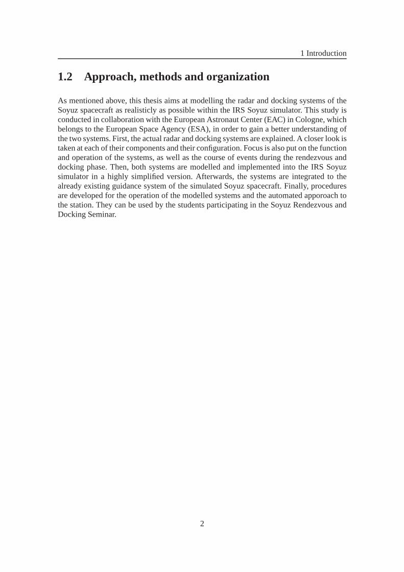
The Soyuz vehicle family is the longest serving manned spacecraft in the world. It wasoriginally designed for the Soviet Manned Lunar program by the Korolyov Design Bu-reau in the 1960s. The spacecraft is launched on the Soyuz rocket from the BaikonurCosmodrome in Kazakhstan (see figure2.1), and can carry a crew of up to three mem-bers. Life support can be provided for 30 days without being docked to a station. Oncedocked, it can stay at the station up to 180 days. At least one Soyuz spacecraft is dockedto the International Space Station at all times as an emergency escape craft.
The first unmanned Soyuz was launched in 1966, the first mannedmission (Soyuz 1) onApril 23, 1967. Over the course of the years, several development steps have been imple-mented to constantly improve the vehicle. The one currentlyin use is the sixth generation,the Soyuz-TMA-M. However, as the IRS simulator is based on the fifth generation, thespecifications of the so-called Soyuz-TMA vehicle are described in the following. TheSoyuz-TMA vehicle was first launched in 2002, and had its lastdescent on April 27, 2012.It was used by the Russian Federal Space Agency to carry Russian cosmonauts and alsoNASA and ESA astronauts to and from the International Space Station. Table2.1 sum-marises the spacecraft specifications.
The spacecraft consists of three parts: the orbital module (habitation), the command mo-dule (used for reentry) and the service module (with solar panels attached), as shownin figure 2.2. Only the command module is reusable and returns back to Earth with thecrew. Both orbital and service module are single-use only. They are jettisoned during thedescent phase and burn up in the atmosphere during reentry.
Theorbital module OMis a spheroid pressurized module and is also called the habitation
3
2 Description of the modelling problem
Figure 2.1.Soyuz rocket launch from Baikonour Cosmodrome. Image courtesy of NASA.
Dimensions Length:7.48mMax. diameter:2.72m
Span (solar array) 10.70mTotal mass 7.2 tCrew 3Launch vehicle Souyz-FGLanding Systems Parachute, retro rockets; landing on landManufacturer RKKReentry acceleration5− 8 g
Table 2.1.Soyuz-TMA spacecraft specifications [3].
4

2 Description of the modelling problem
orbital module
command module
service module
Figure 2.2.Soyuz TMA vehicle with orbital module, command module and service module.Image courtesy of NASA.
section. Figure2.3 shows the module from the inside. It is mostly used as storageforequipment not needed during reentry, e.g. cameras and experiments. The kitchen and atoilet are also located in the orbital module, as well as the radar system KURS, the lifesupport systems and the docking system. It has a length of3m, a diameter of2.25m anda habitable volume of4.8m3. At its far end, it contains the docking port. The hatch at theother end, which connects the orbital and the command module, can be sealed, turningthe orbital module into an airlock, in case the crew needs to exit the vehicle when it is notdocked to the station. There is an additional hatch on one of the sides, through which thecrew exits during an extra-vehicular activity (EVA). This side hatch is also used by thecrew to enter the vehicle on the launch pad.
Thecommand module CMis also a pressurized module and is the only one returning toEarth at the end of the mission. During ascent, descent and landing, the crew is seatedinside the command module. During reentry, the module is protected by an ablative heatshield. First, it is slowed down by the atmosphere. At an altitude of9 km, a breakingparachute opens and at7.5 km altitude, the main parachute slows the vehicle down evenfurther (see figure2.4). 1m above the ground, the solid-propellant breaking engines igniteto ensure a soft landing.
The command module also serves as the cockpit of the Soyuz vehicle and contains controlpanels, which are depicted in figure2.5. Additionally, it holds life support systems andan independent guidance, navigation and control system (much simpler than the mainone in the service module). These systems are used during thereturn flight to Earth,after the module has separated from the service module. Moreover, it also contains a
5

2 Description of the modelling problem
Figure 2.3. Inside view of the orbital module. Image courtesy of NASA.
Figure 2.4.Command module with landing parachute. Image courtesy of NASA.
6

2 Description of the modelling problem
Multi-function displays (MFDs)
Rotational hand controllerTranslational hand controller
Periscope monitor
Figure 2.5.Control panel inside the command module. Image courtesy of NASA.
propulsion system for attitude control during reentry. It has a periscope to allow the crewto see the docking target on the station or the Earth below. The module is2.4m long,has a diameter of2.17m and a habitable volume of3.5m3. A payload of up to50 kgcan be returned to Earth. This value increases to150 kg if only two crew members arepresent. The crew tasks usually contain the surveillance ofcritical parameters like cabinpressure or oxygen levels. During the automated docking process to the station, the crewmembers supervise the correct operating sequence by constantly ensuring that all controlparameters stay within certain limits and all systems work properly. In case the automateddocking fails, the crew can also dock manually, using the hand controllers. Figure2.6shows crew members inside the command module together with aprinted version of theprocedures, which contains a detailed description of all possible crew tasks and which thecrew follows step by step at all times. The figure also illustrates how little free space isavailable in the module.
Theservice module SMis the only non-pressurized module. It contains sytems for ther-mal control, power supply, radio communications, radio telemetry, as well as instrumentsfor orientation and control. In addition to that, it also contains the combined propulsionsystem KDU. The module itself has a length of2.26m and is2.15/2.72m in diameter.The solar arrays are also attached to this module. They have atotal span of10.6m, andwith a surface of10m2 they can produce a power of1 kW. The KDU is a pressure-fedpropulsion system, which uses bi-propellant liquid-fuel reactive thrusters. As propellants,an oxidizer (nitrogen tetroxide) and fuel (non-symmetrical dimethylhydrazine) are usedand they are stored separately in different tanks. There is an orbital maneuvering engi-ne (SKD), and twenty-eight approach and attitude control thrusters (DPO). Twelve of
7

2 Description of the modelling problem
Figure 2.6. Crew members inside command module reading procedures. Image courtesy ofESA.
XLVLH
ZLVLH
Flight Direction
Vehicle Orbit
YLVLH
(a)
XLOSYLOS
ZLOS
Flight Direction
Vehicle Orbit
Station Orbit
(b)
Figure 2.7.Vehicle orienation in space: (a) LVLH; (b) LOS.
the latter are DPO-M (small thrusters) and sixteen are DPO-B(large thursters). They aresupplied from two fully redundant manifolds: the first manifold supplies propellant tofourteen of the DPO-B and six of the DPO-M thrusters (DPO-M1); the second manifoldsupplies two of the DPO-B and six of the DPO-M thrusters (DPO-M2). The small DPO-M1 and DPO-M2 thrusters are only used for vehicle attitude, whereas the large DPO-Bthrusters are used for both attitude and translation.
While in orbit, the vehicle can be commanded into different orientations. The two mainorientations are called LVLH (Local Vertical, Local Horizontal) and LOS (Line of Sight).Both orientations are shown in figure2.7. LVLH is acquired during phasing and rendez-vous. When the vehicle starts getting closer to the station,LOS is acquired. Only in thisorientation, the main radar antennas can measure all the parameters correctly.
8

2 Description of the modelling problem
Flight Direction
Vehicle Orbit
Station Orbit
ρ, ρ'
(a) (b)
Figure 2.8. Measured relative motion parameters: (a) rangeρ and radial closing rateρ′;(b) heading attitudeη, pitch attitudeϑ and line of sight angular ratesΩy andΩz.
2.1.2 Radar system KURS
The radio technical rendezvous system KURS measures relative motion parameters bet-ween the Soyuz vehicle and the station during rendezvous, docking and re-docking, thusenabling automated rendezvous and docking to the station. The measured parameters aredepicted in figure2.8and listed below:
• rangeρ
• radial closing rateρ′
• heading attitudeη
• pitch attitudeϑ
• heading bearingηΠ
• pitch bearingϑΠ
• roll misalignment angleγ
• line of sight angular rateΩ
The heading and pitch bearing,ηΠ andϑΠ, determine the chaser (Soyuz) position in thetarget (station) coordinate system. This means they are thesame angles as in figure2.8b,except with Soyuz and ISS positions swapped. The roll misalignment angleγ is the relati-ve roll angle between the station’s docking port and the vehicle.Ω is the LOS angular ratevector and consists ofΩy, the pitch attitude rate, andΩz, the heading attitude rate. TheKURS system consists of a total of five antennas (see table2.2), which are mounted onthe orbital and on the service module. Figure2.9highlights the antennas on the vehicle.
Depending on the vehicle orientation with respect to the station, the operating range ofthe KURS system changes. When both the vehicle and the station are not pointed at eachother, the range is only50 km. As soon as the vehicle is pointed at the station, but the
9

2 Description of the modelling problem
Figure 2.9.KURS antennas on the Soyuz vehicle. Image courtesy of NASA.
station still has an arbitrary orientation, the operating range increases to200 km. This isthe usual case during rendezvous phase. In case both vehicles are pointed at each other,the operating range is as high as400 km. When the vehicle is pointing at the station du-ring phasing, it is actually not pointed at the desired docking port, but at either one of thestation’s KURS antennas (XPDR antennas) positioned on eachfar end of the solar panelof the Zvesda module. Only when the vehicle is close to the station, the LOS orientati-on is aiming at the KURS antennas of the selected docking port, which are part of theinstrument docking system (IDS).
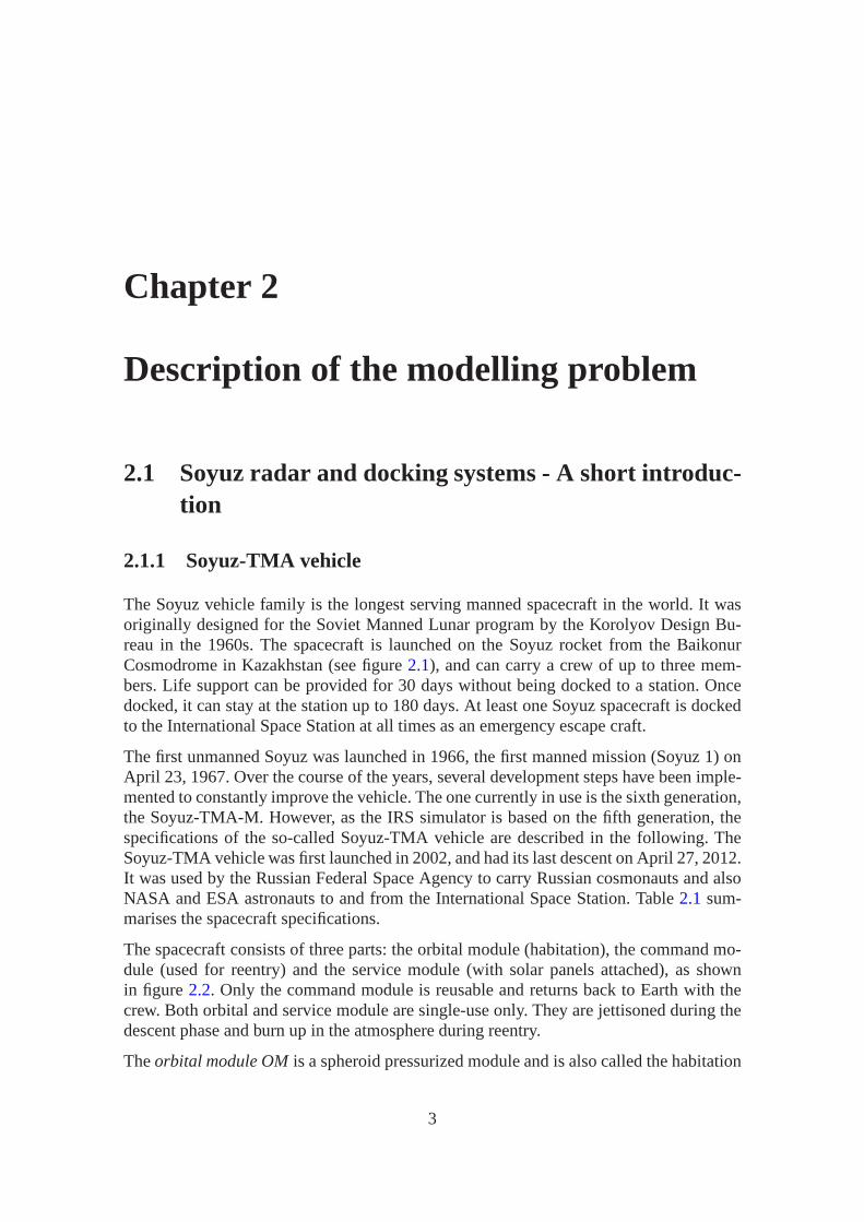
The electronics are made of two identical sets, KURS1 and KURS2. They each containamongst others a filter, a receiver, a logic unit, and an interface exchange unit, as shownin figure 2.10. When the system is activated, both sets are tested and KURS1is chosenby default. Both crew and ground control can command the KURSsystem and observedisplayed commands.
There are several operating modes of the KURS system: thelong testandshort testmode,which are assumed during the two test phases, theSNCmode (“Target Acquired”), assu-med after KURS has detected a signal from the station for the first time,Lock-onmodestarts when the vehicle is in LOS orientation and is auto-tracking the station, andfinalapproachis assumed once the vehicle is pointing towards the docking port instead of theKURS antenna positioned on the far end of the solar array.
Antenna DescriptionAKR1 / AKR2 receive the signal “Target Acquired”, measureρ andρ′
2AO measuresη andϑ, used for LOS orientation, retracted before dockingAKR3 operates together with 2AOACΦ1 measuresρ, ρ′, η, ϑ, γ, ΩACΦ2 measures bearing anglesηΠ, ϑΠ
Table 2.2.Description of KURS antennas.
10
2 Description of the modelling problem
Set 1
Set 2
Logic unit
unitunit
Figure 2.10.KURS system overview
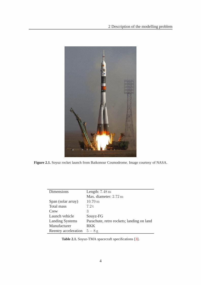
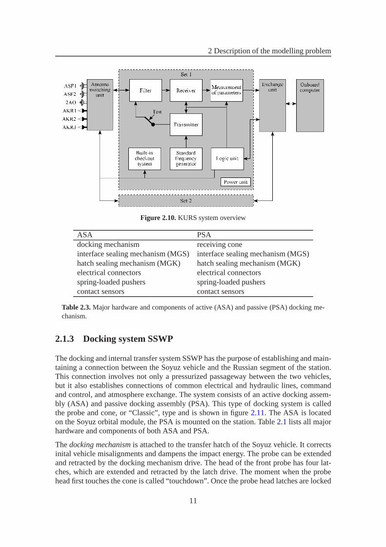
ASA PSAdocking mechanism receiving coneinterface sealing mechanism (MGS) interface sealing mechanism (MGS)hatch sealing mechanism (MGK) hatch sealing mechanism (MGK)electrical connectors electrical connectorsspring-loaded pushers spring-loaded pusherscontact sensors contact sensors
Table 2.3.Major hardware and components of active (ASA) and passive (PSA) docking me-chanism.
2.1.3 Docking system SSWP
The docking and internal transfer system SSWP has the purpose of establishing and main-taining a connection between the Soyuz vehicle and the Russian segment of the station.This connection involves not only a pressurized passagewaybetween the two vehicles,but it also establishes connections of common electrical and hydraulic lines, commandand control, and atmosphere exchange. The system consists of an active docking assem-bly (ASA) and passive docking assembly (PSA). This type of docking system is calledthe probe and cone, or “Classic”, type and is shown in figure2.11. The ASA is locatedon the Soyuz orbital module, the PSA is mounted on the station. Table2.1 lists all majorhardware and components of both ASA and PSA.
Thedocking mechanismis attached to the transfer hatch of the Soyuz vehicle. It correctsinital vehicle misalignments and dampens the impact energy. The probe can be extendedand retracted by the docking mechanism drive. The head of thefront probe has four lat-ches, which are extended and retracted by the latch drive. The moment when the probehead first touches the cone is called “touchdown”. Once the probe head latches are locked
11

2 Description of the modelling problem
extendable probe
probe head
latch
socket
hatch receiving cone
Figure 2.11.Docking mechanism and receiving cone design. Image courtesy of ESA.
in the socket, the docking mechanism draws both vehicles together and mutually alignsthem.
Thefirst mechanical connectionis established once the probe head with extended latchesenters the receiving socket of the PSA. When the head enters the socket, the latches over-come the force of the springs, which keep the stops in place. The stops prevent the headfrom backing out of the cone socket. To break this connection, either the latches need tobe retracted or the stops have to be unlocked. During an emergency, pyrotechnics separatethe docking mechanism from the hatch cover and the latter remains in the receiving conesocket.
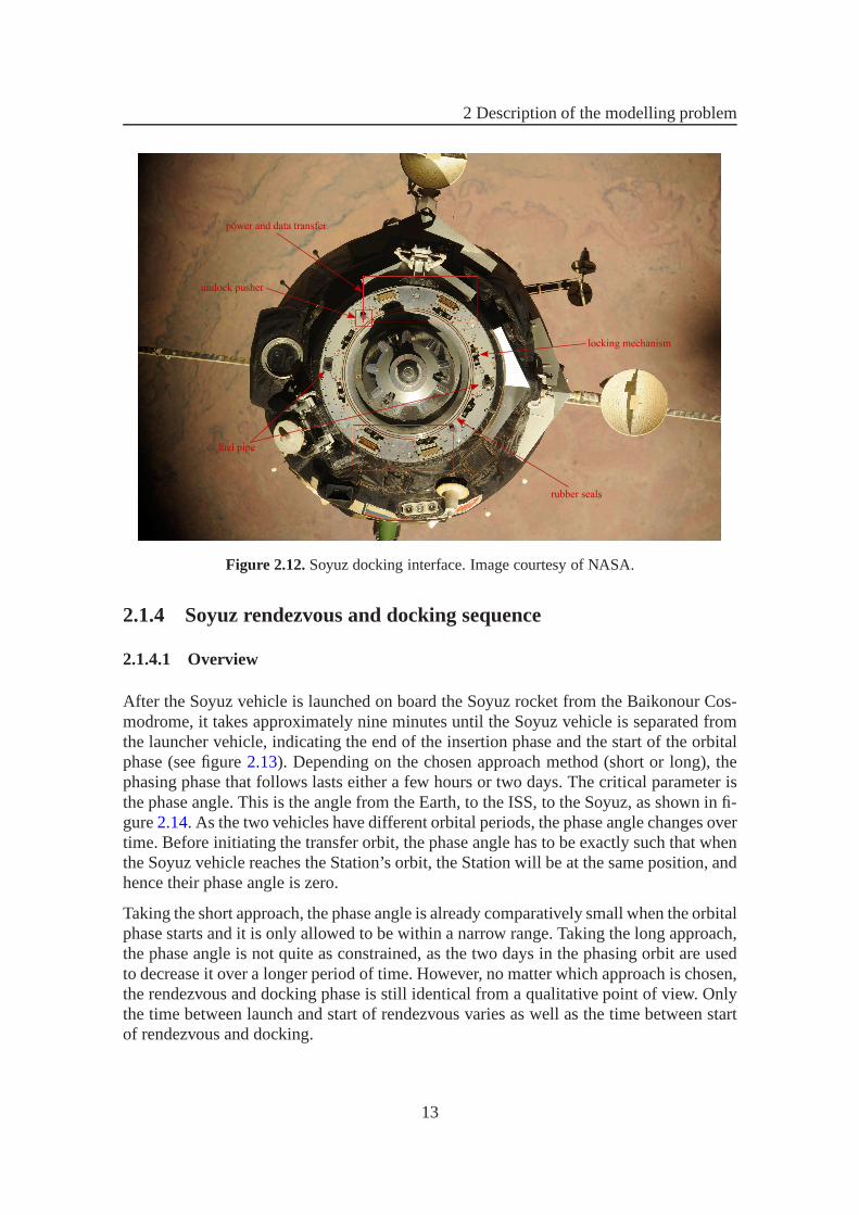
The interface sealing mechanism MGSis identical for both the passive and active part.Figure2.12shows the MGS on the Soyuz vehicle. It contains an interface sealing device,eight locking mechanisms, two rubber seals, and a braided cable connection. Each lockingmechanism has an active and a passive part. Both of them consist of hooks. The activehooks can be controlled by the interface sealing device, thepassive hooks are stationary.They are mounted such that an active hook on the station is always facing a passive hookon the Soyuz vehicle, and vice versa. In case of an emergency,pyrotechnic devices canopen both types of hooks.
Thesecond mechanical connectionis established as the hooks close and the docking ringsare drawn together. The interface is sealed when the rubber sealing rings are compressedby the docking ring on the PSA. This is also called the “rubberon metal” contact. In orderto increase the load-bearing capacity, the crew manually adds several screw clamps.
12
2 Description of the modelling problem
rubber seals
power and data transfer
fuel pipe
undock pusher
locking mechanism
Figure 2.12.Soyuz docking interface. Image courtesy of NASA.
2.1.4 Soyuz rendezvous and docking sequence
2.1.4.1 Overview
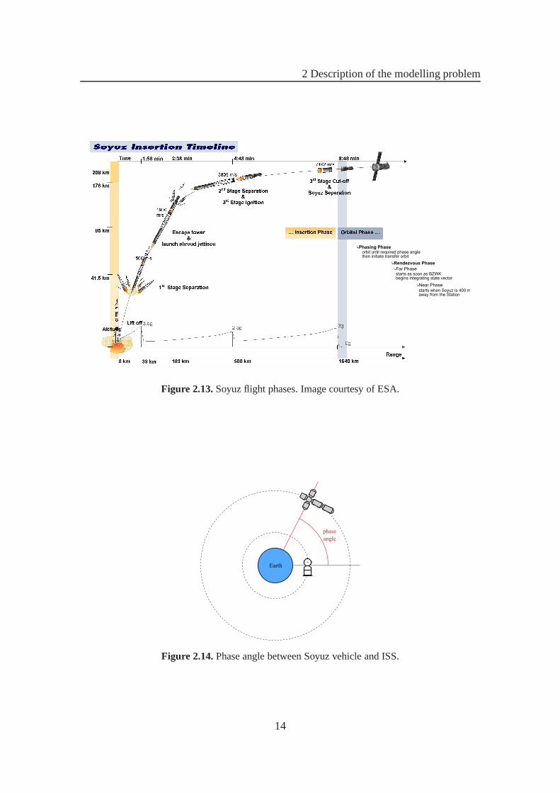
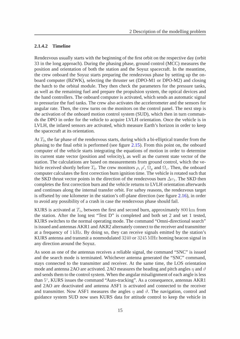
After the Soyuz vehicle is launched on board the Soyuz rocketfrom the Baikonour Cos-modrome, it takes approximately nine minutes until the Soyuz vehicle is separated fromthe launcher vehicle, indicating the end of the insertion phase and the start of the orbitalphase (see figure2.13). Depending on the chosen approach method (short or long), thephasing phase that follows lasts either a few hours or two days. The critical parameter isthe phase angle. This is the angle from the Earth, to the ISS, to the Soyuz, as shown in fi-gure2.14. As the two vehicles have different orbital periods, the phase angle changes overtime. Before initiating the transfer orbit, the phase anglehas to be exactly such that whenthe Soyuz vehicle reaches the Station’s orbit, the Station will be at the same position, andhence their phase angle is zero.
Taking the short approach, the phase angle is already comparatively small when the orbitalphase starts and it is only allowed to be within a narrow range. Taking the long approach,the phase angle is not quite as constrained, as the two days inthe phasing orbit are usedto decrease it over a longer period of time. However, no matter which approach is chosen,the rendezvous and docking phase is still identical from a qualitative point of view. Onlythe time between launch and start of rendezvous varies as well as the time between startof rendezvous and docking.
13
2 Description of the modelling problem
Phasing Phase
Rendezvous Phase
Far Phase
Near Phase
orbit until required phase anglethen initiate transfer orbit
starts as soon as BZWK begins integrating state vector
starts when Soyuz is 400 maway from the Station
Figure 2.13.Soyuz flight phases. Image courtesy of ESA.
phase
angle
Figure 2.14.Phase angle between Soyuz vehicle and ISS.
14
2 Description of the modelling problem
2.1.4.2 Timeline
Rendezvous usually starts with the beginning of the first orbit on the respective day (orbit33 in the long approach). During the phasing phase, ground control (MCC) measures theposition and orientation of both the station and the Soyuz spacecraft. In the meantime,the crew onboard the Soyuz starts preparing the rendezvous phase by setting up the on-board computer (BZWK), selecting the thruster set (DPO-M1 or DPO-M2) and closingthe hatch to the orbital module. They then check the parameters for the pressure tanks,as well as the remaining fuel and prepare the propulsion system, the optical devices andthe hand controllers. The onboard computer is activated, which sends an automatic signalto pressurize the fuel tanks. The crew also activates the accelerometer and the sensors forangular rate. Then, the crew turns on the monitors on the control panel. The next step isthe activation of the onboard motion control system (SUD), which then in turn comman-ds the DPO in order for the vehicle to acquire LVLH orientation. Once the vehicle is inLVLH, the infared sensors are activated, which measure Earth’s horizon in order to keepthe spacecraft at its orientation.
At T0, the far phase of the rendezvous starts, during which a bi-elliptical transfer from thephasing to the final orbit is performed (see figure2.15). From this point on, the onboardcomputer of the vehicle starts integrating the equations ofmotion in order to determineits current state vector (position and velocity), as well asthe current state vector of thestation. The calculations are based on measurements from ground control, which the ve-hicle received shortly beforeT0. The crew monitorsρ, ρ′, Ωy andΩz. Then, the onboardcomputer calculates the first correction burn ignition time. The vehicle is rotated such thatthe SKD thrust vector points in the direction of the rendezvous burn∆v1. The SKD thencompletes the first correction burn and the vehicle returns to LVLH orientation afterwardsand continues along the internal transfer orbit. For safteyreasons, the rendezvous targetis offseted by one kilometer in the station’s off-plane direction (see figure2.16), in orderto avoid any possibility of a crash in case the rendezvous phase should fail.
KURS is activated atT1, between the first and second burn, approximately800 km fromthe station. After the long test “Test D” is completed and both set 2 and set 1 tested,KURS switches to the normal operating mode. The command “Omni-directional search”is issued and antennas AKR1 and AKR2 alternately connect to the receiver and transmitterat a frequency of1 kHz. By doing so, they can receive signals emitted by the station’sKURS antenna and transmit a nonmodulated3240 or 3245MHz homing beacon signal inany direction around the Soyuz.
As soon as one of the antennas receives a reliable signal, thecommand “SNC” is issuedand the search mode is terminated. Whichever antenna generated the “SNC” command,stays connected to the transmitter and receiver. At the sametime, the LOS orientationmode and antenna 2AO are activated. 2AO measures the headingand pitch anglesη andϑand sends them to the control system. When the angular misalignment of each angle is lessthan5, KURS issues the command “Auto-tracking”. As a consequence, antennas AKR1and 2AO are deactivated and antenna ASF1 is activated and connected to the receiverand transmitter. Now ASF1 measures the anglesη andϑ. The navigation, control andguidance system SUD now uses KURS data for attitude control to keep the vehicle in
15

2 Description of the modelling problem
Parking Orbit
Earth
Station Orbit(intermediate)
Transfer Orbit
Incident Trajectory
V1
V2
V3
Vcorr
T0
T1
Figure 2.15.Far phase of rendezvous.
target offset: 1 km
target offset: 750 m
target offset: 300 m
projected Soyuztrajectories
off-plane
direction
flight direction
orbital
plane
Figure 2.16.Target offset during rendezvous phase.
16

2 Description of the modelling problem
y
z
y
z
y
z
[source: BZWK][source: MCC] [source: KURS]
Kalman
filter
Δq=|qBZWK
- qKURS
|
corrected state vector qKAL
y
z
[source: Kalman filter]
integrated state vector qBZWK measured state vector qKURSinitial state vector qMCC
Figure 2.17.Block diagram of Kalman filter and its parameters.
LOS orientation, instead of predictions from the onboard computer. The measured anglescorrespond to remaining misalignments which SUD needs to correct. At the same time,the measurement channels for the relative distance and closing rate,ρ andρ′, respectively,are activated. Once the vehicle receives measurements forρ andρ′, the command “Lock-on” is issued. Now the vehicle KURS system is able to measureρ, ρ′,Ωy andΩz. Then, theonboard computer starts a Kalman filter on the integrated state vector to match it with themeasured values and correct its prediction, as shown in the block diagram in figure2.17.
Regardless of whether “Lock-on” has already been issued or not, the motion control sy-stem determines the next burnvcorr, which usually takes place approximately a quarterorbit after the first large engine burnv1. As this is only a small correction burn, only theDPO-B engines are employed and the vehicle does not have to change its orientation forthe burn. After the correction burn is completed, the vehicle continues along the internaltransfer orbit to the offset target.
At the specific time that the onboard computer has calculatedfor firing the second burnv2, the vehicle is rotated in the correct attitude and the SKD isfired for the calculated burnduration. Afterwards, LOS orientation is acquired again. The vehicle then continues to theoffset target, which is still located one kilometer from thestation in off-plane direction.The completion of both of the burnsvcorr andv2 marks the timeT2, at which the distanceto the station is around60−80 km. If by this time, KURS has not generated the command“Lock-on”, a switch is made to the alternate system atT2+2min. That is, if KURS 1 wasrunnning so far, it is switched to KURS 2 (if this one is functional). At at relative distanceof ρ = 15 km, a short test on the “hot” KURS system is performed in order toprevent anyerrors in relative range measurements during the close approach.
Finally, the onboard computer calculates the firing time forthe third engine burnv3. Thisrendezvous burn, which cancels out all relative velocity between the vehicle and the target,actually consists of two parts. During the first part, the vehicle is rotated almost by180
and the SKD engine is used to rapidly decrease the relative velocity between the twovehicles. The offset target is first reduced to a distance of750m from the station, thento 300m. The second part ofv3 itself again consists of several smaller burns of the DPOengines. The completion of the third engine burn also marks the end of the far phase of
17

2 Description of the modelling problem
Flight Direction
400 m
150 m
Figure 2.18.Near phase of rendezvous.
the rendezvous.
In order to transition to the near phase, certain requirements need to be fulfilled: Therelative distanceρ has to be less than400m, the relative velocityρ′ less than2m/s andthe relative angular rate has to be smaller than0.3 ([2]). The vehicle then performs aflyaround to align the vehicle axis with the station axis (seefigure2.18, while decreasingthe relative distance toρ = 150m and targeting the antenna on the station, whose signalwas used as a target for the “Lock-on” command. Once the flyaround is completed, thevehicle shortly enters the station keeping mode, keeping both the relative velocityρ′ andthe angular ratesΩy andΩz at zero.
KURS then switches to “Final Approach” mode and shifts from being locked on to the ho-ming beacon antenna of the station to the KURS antenna on the selected station dockingport. As a consequence, the vehicle acquires the new LOS orientation. A second flyaroundis executed, this time while keeping the relative distance of 150m. Once the vehicle is ali-gned with the desired docking port, it performs station keeping again. The crew thenissues the final approach command and the vehicle approachesthe station while maintai-ning the LOS orientation relative to the docking port. At a relative distance of40m, the2AO antenna boom automatically retracts, as docking with the antenna still deployed isprohibited due to safety reasons. As soon as the probe head touches the cone, the motioncontrol system enters the “touchdown” mode, which causes the thrusters to push the ve-hicle forward. Due to the present microgravity, two spacecraft touching each other mightlead to the effect of the two vessels pushing themselves awayfrom each other. Therefore,upon touchdown, the thrusters give the Soyuz an extra push, and the two vehicles finallydock.
As soon as the probe head is captured by the station socket, the command “capture”is generated, KURS shuts down and the motion control system enters the “free drift”
18

2 Description of the modelling problem
mode. This prevents the thrusters from trying to correct thevehicle attitude while theprobe head gets retracted. Figure2.19shows the Soyuz vehicle and the ISS in the dockedconfiguration. Twenty minutes after the vehicle and stationdocking mechanisms engage,the motion control system is automatically deactivated. The crew then performs a seriesof leak checks before they are finally able to open the hatch which connects them to thestation, where they are usually greeted by the current crew of the station.
2.2 Soyuz simulator at the Space Systems Institute
2.2.1 Soyuz simulator facilities
The project “Soyuz simulator at the Space Systems Institute” started in 2007 under the di-rection of Prof. Ernst Messerschmid, who is a former astronaut and was in space in 1985.The very first version of the simulator consisted of two off-the-shelf personal computersand control sticks, which were directly purchased from the Gagarin Cosmonaut TrainingCenter (GCTC) in Russia. In summer 2008, the first training seminar for students hadan overwhelming response and over the course of the past years, the simulator has beenupgraded step by step.
Today, the simulator includes a model of the Soyuz capsule, which offers the students asemi-realistic cockpit environment, and a simplified ground station for the supervision bythe flight instructor. The capsule is an original sized modelof the orbital module of theSoyuz spacecraft and was developed at EAC/ESA in Cologne fortheir own simulator. Ithas a basic diameter of2.3m and a height of2m. For an easy access, the capsule can beopened in the middle, as shown in figure2.20.
Inside, the capsule features all the important elements of the cockpit, as indicated in fi-gure 2.21: First, there is the integrated operational panel including two multi-functiondisplays (MFD) and several switches. The view through the periscope of the vehicle issimulated on another monitor, allowing to see what is in front of the spacecraft. For mo-tion control around all six degrees of freedom, two control sticks are installed. The leftstick controls all translational movements, i.e. forward/backward, right/left and up/down.All rotations around the vehicle’s three axes, i.e. pitch, yaw and roll, are controlled by theright stick.
The crew is seated in three rather narrow seats, with the flight engineer on the left, themission specialist on the right, and the captain/pilot in the center. However, during the“Soyuz Rendezvous and Docking” seminar, usually only the pilot’s seat is occupied.
Figure 2.22 shows the ground control station with its several personal computers andscreens. This is where the simulator framework, the free software “Orbiter Space FlightSimulator”, developed by Dr. Martin Schweiger, is run. For the software to include thecontrol of the cockpit and the Soyuz systems, so called add-ons were implemented atthe IRS. These add-ons consist of approximately 25,000 lines of code. A more detailed
19

2 Description of the modelling problem
Figure 2.19. Soyuz vehicle docked to the International Space Station. Image courtesy ofNASA.
20

2 Description of the modelling problem
Figure 2.20.Model of Soyuz capsule at the Space Systems Institute. Imagecourtesy of IRS.
Figure 2.21.Simulator cockpit. Image courtesy of IRS.
21

2 Description of the modelling problem
Figure 2.22.“Ground station” of the IRS simulator. Image courtesy of IRS.
description of the Orbiter software can be found in section2.2.2. More information on theimplementation at the IRS can be found in [8].
The flight instructors can load different flight scenarios from the ground control stationand supervise the practicing student. They can also intervene a running simulation toassist the student from outside the cockpit in case of any deviations from the flight plan,as well as purposely cause a malfunction in a subsystem of thevehicle.
2.2.2 Orbiter space flight simulator
Orbiter is a real-time 3D space flight simulator for Windows PC, developed to simulatespace flight using realistic Newtonian physics. Its conceptis very similar to traditionalflight simulator softwares, however without being limited to atmospheric flight. Orbiterwas first released in November 2000, and its latest version was launched in August 2010.Originally, the software was developed by Dr. Martin Schweiger, a senior research fel-low at the University College London, who was unsatisfied with space flight simulatorslacking in realistic physics-based flight models. It is written in C++ and uses DirectX for3D rendering.
In Orbiter, the user can experience manned and unmanned space flight missions from apilot’s point of view. This includes all phases of a mission:Launch, orbital insertion, ren-dezvous with space stations, deploy and recapture of satellites, reentry and landing on aplanetary surface. However, there are no predefined missions to accomplish or opponentsto be defeated. Moreover, Orbiter is about learning what is involved in real space flight:What do you need to know when you want to launch into a certain orbit? What is im-portant when trying to rendezvous with a space station? Or what are the difficulties when
22

2 Description of the modelling problem
flying to another planet?
The Orbiter software itself is basically just a skeleton that defines the physcial model.Included in the core software are a few spacecraft and most ofthe bodies in our solarsystem. Even though the program source code is not published, in return there is an ex-tensive Application Programming Interface (API), which allows users to contribute to thesoftware by creating so-called add-ons. A multitude of suchadd-ons has been developedby the Orbiter community and is largely available on the web:There are additional space-craft, celestial bodies, enhanced instruments etc.. The Soyuz and ISS models used at theIRS (and among others also further developed as part of the present thesis) are basicallyalso add-ons to the core software.
23
Chapter 3
Method and tools
3.1 Object-oriented programming
The simulator framework, i.e. the Orbiter space flight simulator, is written in the object-oriented programming language C++. The following section aims at giving a short in-troduction to both the object-oriented programming paradigm and the C++ programminglanguage, in order to gain a better understanding of the underlying programming conceptsof the IRS simulator and the advantages they bring about.
Different approaches to programming have developed over time and the resulting lan-guages are defined by differentiating between paradigms. There are four main paradigms([5]): imperative, functional, object-oriented and logic programming. Different program-ming paradigms use different ways to model the information and how it is processed andthey have different concepts on how information and processing interact. Some languagesare designed to support only one particular paradigm, whileother languages can supportmultiple paradigms. As the Orbiter code is mainly1 object-oriented, only this paradigmwill be explained in more detail hereafter and an elaborate description of the other para-digms is omitted.
Object-oriented programming derives its basic principlesfrom real world processes andobjects. These processes are modelled through acting individuals, who perform and assigntasks. In object-oriented programming, those individualsare called objects.
An object is an entity consisting of a data structure in concert with a definition of relatedoperations. All of the used data is distributed among the objects, and additionally, there areno global operations. Each operation directly belongs to anobject and can only be engagedby sending a message to the respective object. This technique is called encapsulation. Thevariables defined locally for an object are called attributes and the local operations arecalled methods. The description of those local methods is usually done using proceduralprogramming.
1The code also contains procedural parts while at the same time lacking some typical object-orientedconcepts, such as streams.
24

3 Method and tools
An object has a well-defined interface, which describes the properties of the object: themessages or operators, which the object understands and a list of those attributes acces-sible from outside the object. Ideally, attributes can onlybe accessed through a methodand the object has total control over its data. This technique can rule out inconsistentor unphysical object states. Objects are classified depending on their interface and theseinterfaces can be inherited by subsidiary classes.
A program can be understood as a system of cooperating objects. These objects have astate, a life span and they exchange messages with each other. While an object is proces-sing a received message, it can change its own state, send messages to other objects (oritself), create or destroy other objects. Objects behave like items in the material world;they are said to have an identity: An object cannot be presentat two places at the sametime and it can change its state while still staying the same object. Just like a propellanttank can either be full, empty or somewhere in between, and still stay the same propel-lant tank. This is also the main difference to mathematical objects like numbers and facts.Object-oriented programming models the real world as avirtual world. Programs try toreflect as far as possible (or as necessary) that part of reality they are going to treat.
A central thought of object-oriented programming is the separation of the task assignmentand the task completion. If one object needs a task to be done,it will look for anotherobject who is capable of performing the task. It then sends a message to the object whichhas the corresponding method for the task completion. The client object is ignorant ofthe details on how the executing object performs the task. This principle is also calledinformation hiding. The executing object receives the message and has the correspondingmethod to respond to it and this is all the client object needsto know. An example forthis is the communication between the Soyuz’ OM and the KURS system. When the OMwants to know the LOS angles, it asks KURS to compute them and KURS provides thedesired answer. The OM only knows that KURS has a method to calculate those anglesand it knows what information is required by KURS to do so. It does not know however,what particular calculations are performed.
Another important principle of object-oriented programming is classification and inheri-tance. A class defines all the methods and properties, which all its objects have in com-mon. Classes can be organized hierarchically. Superior classes only own those properties,that the subsidiary classes/objects have in common. Subsidiary classes inherit propertiesand methods from the superior classes. Those properties andmethods only need to bedefined once for the superior class. However, inherited methods can be further adjustedand defined in more detail in the respective class. In Orbiter, for example, the OM, SMand CM are modelled as sub-classes of the “VESSEL3” class, which is itself derived fromthe “VESSEL” class. Thus, the OM, SM and CM inherit all the methods and propertiesof the superior “VESSEL” class, and in addition, they each have their own specializedproperties.
All in all, object-oriented programming offers an easy way to enhance and reuse existingprograms. Due to the application of the messaging system, the connection between aservice request (sending of a message) and the method (executable part of the program)only happens during runtime, which makes this a very dynamicprogramming paradigm.
25

3 Method and tools
Objects are easy to extend and specialize using additional attributes and methods, whichonly lead to a larger interface. However, extended objects still match the old interface,which makes extended objects easy to implement.
3.2 Introduction to C++
The C++ programming language development started in the Bell Labs in Murray, NewJersey, in 1979 and aimed at extending the C programming language by adding object-orientation. It is a statically typed, compiled, general-purpose, case-sensitive, free-formprogramming language. Note that just because a program is written in C++, this doesnot automatically imply object-orientation. C++ supportsprocedural, object-oriented andgeneric programming.
For the Orbiter space flight simulator, the C++ language holds many advantages ([6]):It offers a simple and safe usage and a high reusability. It enables easy-to-maintain andwell-written code, which makes the simulator easy to extendand enhance without greatexpense. Additionally, C++ is a compiled language, meaningthat programs can be dis-tributed to people who do not need to have the respective compiler in order for them touse the program. This makes the simulator a portable programwhere the end user doesnot have to be a software developer to be able to use it. But on the other hand, it stillenables the user to enhance the program by the so-called add-ons if he desires to do so.How this is done exactly is described in the following section about the Orbiter SoftwareDevelopment Kit (SDK).
3.3 Programming tools
The Orbiter SDK can be downloaded from the same website as thesimulator itself [13]. Itcontains the application programming interface (API) in the form of some libraries, codeexamples, a few utilities and useful documentation ([12, 10, 11]). The API includes theinterface methods; a set of functions for getting and setting general simulation parametersin a running Orbiter simulation session. These methods can be used by all types of pluginmodules and their name always starts with “oapi”.
Furthermore, the Orbiter API (OAPI) also contains the properties and methods of the“VESSEL” class and its two derivatives, “VESSEL2” and “VESSEL3”. These classes arethe base classes for creating new vessels, e.g. the Soyuz’ orbital module. For creating newmulti-function display modes, developers need the “MFD” and “MFD2” classes, whichare also part of the API.
In addition to the API provided by Orbiter, there is the so-called “oapiExt”, a functionlibrary developed at the IRS [7]. It was developed for modelling the Soyuz spacecraft, butthe code itself is generic and can also be used in other vessels. It contains for example an
26

3 Method and tools
autopilot (AP) and a timer for counting down the simulation time. More information canbe found in [7].
All code developing, debugging and management is done usingMicrosoft Visual Studio2010 (MSVS), which is an integrated development environment (IDE). It contains theIDE Microsoft Visual C++ (MSVC), which is designed for C++ programming tasks.
27

Chapter 4
Model and implementation
4.1 Overview
This chapter describes how the existing simulator code was enhanced in order to imple-ment the Soyuz KURS system. First, the so-called back end of KURS is explained: Theinternal parts of the systems, the different operating modes, etc.. Second, the KURS frontend, i.e. the user interface, is described: The different views on the MFD, the informationavailable to the pilot and the decisions he has to make with respect to KURS. Finally, theprocedures are presented. These are the checklists tellingthe pilots for example, whichparameters they need to monitor and which systems they have to activate or deactivateat what time. As stated in chapter1, originally, also the implementation of the internaldocking and transfer system was part of the present thesis. Throughout the project howe-ver, it became clear that focus was going to be put on the implementation of the radarsystem. This seemed the more relevant/interesting system for the aerospace engineeringstudents participating in the Soyuz Seminar to be adressed in this time-constraint thesis.
A general concern while performing the implementation of the systems is the questionhow close the model should resemble the real system. On the one hand, the simulatoraims at providing the students with a realistic environmentto experience and understandthe challenges and tasks of a pilot as close to reality as possible. On the other hand, thetraining students should not be overwhelmed by the complexity of the simulator and theyshould be able to acquire appropriate spacecraft operationskills over the short trainingperiod of a few weeks. Finding the right balance between being simple and being realistic,and between what is feasible and what is reasonable, is one ofthe many challenges of thepresent thesis.
28

4 Model and implementation
OFF LONG TEST
SEARCH
SNC
LOCK-ON
SHORT
TEST
APPROACH
FLYAROUND
FINAL
KURS deactivation via pilot
Nominal change of operating mode
Loss of navigation signal
Loss of LOS attitude
Figure 4.1.Schematic of KURS operating modes.
4.2 KURS back end
As mentioned above, the KURS back end basically consists of everything that the user,i.e. the pilot, cannot see or manipulate directly. The scopeof the back end goes from themodelling of the antenna signal range to the calculation of the relative motion parametersup to the commands sent to the autopilot. Depending on the current vehicle state in therendezvous and docking sequence, KURS has several different operating modes. Thesemodes determine for example which parameters are currentlyevaluated and what actionshave to be taken. As the KURS system usually acquires these modes in a chronologicalorder, from the far phase to near phase to mechanical docking, they will be described in thesame order in the following. Figure4.1 illustrates the relationship between the differentmodes.
The system is desigend such that it is turned on after the rendezvous far phase has started.This means, that at this point, the vehicle has already left its insertion orbit and is in thetransfer orbit. The rendezvous burns are not calculated by KURS, but by the onboardcomputer BZWK, which is part of the motion control system SUD(see figure4.2). TheBZWK then in turn commands the KDU system to perform the burns. As neither theBZWK nor SUD were part of the present thesis, the automatic calculation and executionof the necessary burns is not implemented in the simulator atthis point, but can be addedin the future. Until then, the burns have to be performed manually.
When the KURS system is started in the simulator, it automatically assumes that all an-tennas have been deployed successfully and that the dockingprobe head is fully extended.
The KURS system is implemented in the simulator as aC++ class, and the Soyuz OM
29

4 Model and implementation
Figure 4.2.Functional schematic of the motion control system SUD.
vessel automatically creates an instance of this class whenthe simulation is loaded andinitialized. Before every time step, the OM checks the current operating mode of KURSusing the built-in function of all vesselsclbkPreStep()from the Orbiter API. Dependingon the operating mode, different commands will be executed by the KURS object.
Independent of the current operating mode, the KURS model always determines the cur-rent LOS angles (η, ϑ andΩ). In reality, the angles are either calculated by the BZWKor measured by the KURS system. In the implemented simulatormodel, the values repre-senting BZWK data are calculated from the CM’s center of gravity to the position of thereceived KURS signal transmitter. The “real” measured KURSdata is calculated from theSoyuz KURS antenna to the signal source in the model. Additionally, the range and rangerate (ρ andρ′, respectively) are calculated similar to the BZWK data, i.e. from the CM’scenter of gravity to the target transmitter.
The calculation of the LOS angles from the BZWK system takes place as follows. First,the KURS model determines whether a navigation signal is received, and whether it isfrom the correct transmitter type (XPDR or IDS). Then, the model uses the API functionoapiGetNavPos()to determine the position of the received signal transmitter. Next, itcalculates the position of the CM’s center of gravity in global coordinates via the functionGetGlobalPos(). This function determines the position of a vessel’s centerof gravity andis also part of the OAPI. By subtracting the two positions, the BZWK line of sight isobtained and can be rotated into local Soyuz coordinates. Now the LOS angles can bedetermined. The LOS vector is projected into the vehicle’s orbital plane and using thescalar product of the projected vector and the vehicle’s z-axis (pointing towards the frontof the spacecraft), the azimuth angle can be evaluated. The elevation angle is determinedusing the scalar product of the LOS vector and its projection. Finally, the LOS rates arecalculated via the difference of the angles over the previous time step.
The LOS angles representing measured KURS data are calculated similarly to the BZWKvalues. The only difference is that now instead of the CM’s center of gravity, the positionof the docking port is used. The latter can be determined via OAPI function GetDock-Handle(), which returns the position of the docking port in local vessel coordinates.
30

4 Model and implementation
The KURS data set also contains the pitch and heading bearinganglesηΠ andϑΠ. Acoordinate system is created for the station’s docking portand then the line of sight vectoris expressed with respect to these coordinates. Afterwards, the pitch and heading bearingangles can be calculated in the same way as the previous angles.
Finally, the range and range rate are also calculated. Thesevalues are once again calcula-ted with respect to the CM’s center of gravity. After making sure a signal is received fromthe correct transmitter, the line of sight vector to the station is calculated in local vesselcoordinates. The rangeρ is simply the length of this vector. The range rateρ′ can be de-termined using the OAPI functionGetRelativeVel(), which calculates the relative velocityvector between two vessels. As this vector is with respect tothe global reference frameand contains the relative velocity in all three directions,the actual range rate is the resultof the scalar product of the relative velocity and the line ofsight vector.
4.2.1 “OFF” mode
By default, KURS is in the “OFF” mode. No parameters are calculated and no commandsissued. This mode can be acquired while being in any other operating mode. This meansthat the KURS system can be deactivated throughout the entire rendezvous and dockingsequence (see the black dashed line in figure4.1).
4.2.2 “LONG TEST” mode
Once the system is activated, it automatically goes into the“LONG TEST” mode. Duringthis mode, a long system check of the two KURS systems is simulated by simply stayingin this mode for a predefined amount of time (150 s, [2]) without actually doing anything.For this purpose, theSIMTIMERclass was developed, which enables the system to countdown simulation time.
The “LONG TEST” mode is always acquired after the “OFF” mode.Even if the test hasalready been performed before, and KURS is deactivated while in another mode, the longtest will always be performed again upon (re-)activation ofthe system.
4.2.3 “SEARCH” mode
In the “SEARCH” mode, the KURS model checks whether the OM’s primary navigationdevice receives a signal from the ISS XPDR. By default, each vessel in the Orbiter simu-lator has two built-in navigation devices. Besides, the station’s XPDR frequency can beset in the scenario configuration file (see [9] for more details on how to edit scenarios).The KURS model is programmed such that by default, the primary navigation device isalready tuned to the ISS XPDR frequency. However, its frequency can still be modifiedby the pilot.
31
4 Model and implementation
The transmitter strength in the Orbiter simulator is modelled such that it drops off withthe square of distance to the transmitter [11],
S = S0/r2, (4.1)
whereS is the received signal strength at the distancer.S0 is set by Orbiter to a value suchthat a receiver will detect a signal strength of1 when it is just in range of the transmitter.
The signal range of the station’s XPDR predefined by Orbiter is longer than the range ofthe real system. Therefore, the implemented model not only checks whether an XPDRsignal is received, but also if it is above the signal strengthSreal that would be received atthe real system’s rangerreal. Both can be done using the OAPI functionsGetNavSource()andoapiGetNavSignal(). To prevent the model from switching back and forth when thereceived signal is just around the threshold, a hysteresis factor is implemented. Thus, asignal is processed as “received” when the signal strength is slightly aboveSreal. On theother hand, when a signal is currently received, it will be processed as “lost” only whenthe signal strength is slightly belowSreal.
Summing up, this means for the “SEARCH” mode: If a signal is received and its strengthis above the required threshold, the KURS model switches to the “SNC” (“Target Acqui-red“) mode. If the KURS model is in any later operating mode, and the signal strengthdrops below the threshold or is lost completely, it always returns to the “SEARCH” mode(see red lines in figure4.1).
4.2.4 “SNC” mode
The “SNC” mode starts as soon as the received XPDR signal is strong enough, i.e. thevehicle is in the range of the transmitter. This condition ischecked for every time stepwhile in “SNC” mode. During this mode, the vehicle is rotateduntil it points towards thereceived signal source. This is achieved using the SUD model(its autopilot, respectively),which is part of the oapiExt, the extended OAPI developed at IRS.
First, the SUD model is passed the target vessel (the station) using the functionSetTar-getObject(). SUD also requests a docking port, but at this point in the rendezvous phase,no docking port has been selected yet. However, the functionprovides an extra option forthis flight phase, in which the center of gravity of the targetvessel is chosen instead of aphysical docking port. Next, a command is issued to the SUD implementation to rotatethe vehicle until it is pointed at the selected docking port (in this case the center of gravi-ty). At the same time, as a secondary constraint, SUD is to maintain the vehicle’s rotationattitude, thus keep its y-axis pointing upwards.
For every time step, as always, the KURS model evaluates the current azimuth and eleva-tion angles and rates of the line of sight. As soon as both azimuth and elevation angle arebelow5, which means the vehicle is aligned with the station, KURS switches to the nextmode: “LOCK-ON”.
32

4 Model and implementation
4.2.5 “LOCK-ON” mode
During the “LOCK-ON” mode, the Soyuz continues its flight towards the station. In rea-lity, this is usually the mode in which the correction and thesecond burn take place. Asmentioned at the beginning of this chapter, these burns are neither computed nor com-manded by the KURS system and therefore are not implemented within the scope of thepresent thesis. On the other hand, however, this allows the KURS model in the simula-tor to operate fully independent of whether these burns are performed manually or not.The only thing that matters to KURS is the attitude of the vehicle and its distance/closingspeed with respect to the target, but not the way this position was acquired.
Just as in the previous modes, the KURS model checks whether an XPDR signal is re-ceived at a sufficient strength before every time step or elsereturns to the “SEARCH”mode. Additionally, while in the “LOCK-ON” mode, KURS also checks whether the lineof sight angles are still below the threshold of5. If this condition fails, KURS returnsto the “SNC” mode (see the yellow lines in figure4.1). As the SUD hasn’t received anycommands otherwise and “LOCK-ON” can only be reached from the “SNC” mode, SUDwill keep the Soyuz pointed at the station’s center of gravity while getting closer to it.
At a relative distance of15 km, the KURS model switches from “LOCK-ON” to “SHORTTEST” mode. After the test is completed, the system returns to “LOCK-ON” and pro-ceeds its approach to the station. Once the Soyuz is within400 m of the station, the“APPROACH” mode is acquired.
4.2.6 “SHORT TEST” mode
The short test is performed very similarly to the long test, except that it is, as in the name,shorter. Just as in the long test, the KURS model uses theSIMTIMERclass to count downthe duration of the test (75 s, [2]). This test will be performed again, should the KURSmodel have to switch back to the “SEARCH” mode in case the transmitter signal is lost.While the test is performed, no KURS data is generated and therefore not available forthe crew to monitor.
4.2.7 “APPROACH” mode
The “APPROACH” mode is acquired once the vehicle is within400 m of the target. Thestart of this mode also marks the beginning of the rendezvousnear phase. Each time step,as in the previous mode, both the received signal strength and the line of sight attitudeare verified and, if necessary, the KURS model switches back to “SEARCH” or “SNC”,respectively.
During the “APPROACH” mode, the vehicle slowly acquires a station keeping positionfacing the XPDR antenna mounted on the solar array of the Zvesda module at a distanceof 150 m. This is achieved by using the motion control system again. First, the maximum
33

4 Model and implementation
relative velocity is set to2 m/s in all directions. Second, SUD is instructed to acquire thestation keeping position.
1 AP_COMMAND cmd;cmd.commandClass = APCMD_TLIMIT;
3 cmd.local = _V(2.0, 2.0, 2.0);pAP->ExecuteCommand(&cmd);
5
cmd.commandClass = APCMD_TPOS;7 cmd.local = vRefApproach;pAP->ExecuteCommand(&cmd);
The exact location of the XPDR signal source on the ISS is not known in the Orbitersimulator. Therefore, the coordinates of this position arepredefined in the KURS model(vRefApproach) with respect to the center of gravity of the target and so faronly representthe correct antenna position when docking to the ISS. When approaching another spacestation of course, where the KURS antenna is positioned somewhere else, these coordi-nates might be different. During the whole process, the motion control system keeps thevehicle pointed at the station’s center of gravity.
At some point during the “APPROACH” mode, the KURS model expects a docking portselection from the user. As soon as a port has been selected, the system switches to the“FLYAROUND” mode, even if the station keeping position in front of the solar array hasnot been reached yet.
4.2.8 “FLYAROUND” mode
During the “FLYAROUND” mode the vehicle is moved from its station keeping positionin front of the XPDR antenna to a station keeping position in front of the selected dockingport at a distance of150 m. As soon as a docking port is selected, the OM’s primarynavigation device is tuned to the IDS signal of the respective port instead of the XPDRfrequency of the station. The KURS model checks whether an IDS signal is recievedand, analogous to the XPDR signal, the signal strength is verified. Just as with the XPDRsignal, a hysteresis has been implemented in order to prevent the system of switching backand forth when the vehicle is on the edge of being in range of the transmitter.
Next, the selected docking port is delivered to the implemented motion control system asthe target docking port instead of the center of gravity of the station. The KURS modelthen commands the SUD model to acquire the station keeping position150 m away fromthe docking port. The maximum relative velocity in any direction during the flyaroundis set to1.5 m/s (FlyArSpeed). As an additional constraint, the KURS model commandsSUD to align the the vehicle’s x-axis with that of the selected port.
AP_COMMAND cmd;2 cmd.commandClass = APCMD_TPOS;cmd.local = _V(0.0,0.0,150.0);
4 pAP->ExecuteCommand(&cmd);
34

4 Model and implementation
6 cmd.commandClass = APCMD_TLIMIT;cmd.local = _V(FlyArSpeed, FlyArSpeed, FlyArSpeed);
8 pAP->ExecuteCommand(&cmd);
10 cmd.commandClass = APCMD_CONSTRAINT;cmd.local = _V(-1.0, 0.0, 0.0);
12 cmd.target = APDIR_REFY;pAP->ExecuteCommand(&cmd);
Now that a docking port has been selected, the line of sight isconsidered to go from theSoyuz vehicle to the docking port instead of the center of gravity of the station. Hence,during the entire maneuver, the vehicle is pointed now to thedocking port instead of thecenter of gravity.
In order to determine the completion of the flyaround, the remaining misalignment andthe remaining relative velocity are measured. First, both the current line of sight vectorand the approach vector of the docking port are determined. The line of sight vector is thedifference between the position of the vehicle and the docking port in global coordinates.The approach direction can directly be accessed through thefunctionGetDockParams()(which is part of the Orbiter API). Then, the cross product ofboth of these vectors iscalculated. If the vehicle was perfectly aligned with the docking port, the result wouldbe zero. However, there are several control loops involved in the simulator, which willalways lead to a residual error. Therefore, in the implemented model, the flyaround isconsidered complete when the result of the cross product is less than0.3 and the relativevelocity is less than0.3m/s in all directions. Finally, KURS waits for a user command toswitch into the “FINAL APPROACH” mode.
4.2.9 “FINAL APPROACH” mode
In the “FINAL APPROACH” mode, the received signal strength of the IDS antenna isverified in every time step. The implemented KURS model commands the SUD imple-mentation to stay aligned with the docking port and adds the constraint that vehicle’srotation should also be aligned with the target. Then, the maximum relative velocity is setto 0.15 m/s in all directions ([1]). Finally, the command is issued to acquire the dockedposition, or basically to move the vehicle to the origin of the port’s coordinate system.
1 AP_COMMAND cmd;cmd.commandClass = APCMD_ALIGN;
3 cmd.local = _V(0.0, 0.0, -1.0);cmd.target = APDIR_REFZ;
5 pAP->ExecuteCommand(&cmd);
7 cmd.commandClass = APCMD_CONSTRAINT;cmd.local = _V(-1.0, 0.0, 0.0);
9 cmd.target = APDIR_REFY;
35

4 Model and implementation
pAP->ExecuteCommand(&cmd);11
cmd.commandClass = APCMD_TLIMIT;13 cmd.local = _V(0.15, 0.15, 0.15);pAP->ExecuteCommand(&cmd);
15
cmd.commandClass = APCMD_TPOS;17 cmd.local = _V(0.0, 0.0, 0.0);pAP->ExecuteCommand(&cmd);
4.3 KURS front end
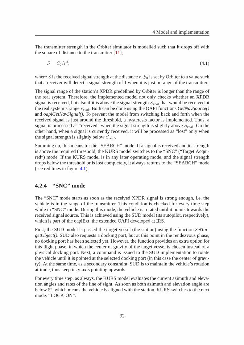
A front end is an interface between the user and the back end. In the IRS Soyuz simulator,the front end consists of the control panel, the periscope screen and the two control sticks.Concerning the implemented KURS model, however, only the MFDs are part of the frontend. The student pilot can interact with KURS through a series of different views. In thereal Soyuz spacecraft, these views are called “format”. Theimplemented views in thesimulator are not identical to the formats, but try to find a balance in the issue describedat the beginning of this chapter about how realistic versus how simple the displayed datashould be.
In the Orbiter simulator, all MFD views belong to theVIEW class, and for each system(KDU, SUD, KURS, etc.) a derived subclass is constructed. Each view can have subviews,which also belong to theVIEW class. Figure4.3shows the super- and subordinate viewsof the KURS view. It should be noted, that one view can actually consist of differentdisplays. That is, even though there is only a single KURS view, different information anddata might be shown on the screen depending on the current KURS operating mode. Thelatter is always displayed in the top center of the screen when in the KURS view. There isone main view, as shown in figure4.4a, through which all implemented instruments of theOrbiter simulator can be accessed. This is also the view the MFD turns to when pressingthe “SEL” button in the bottom center. After selecting “Soyuz Systems”, the user will beable to choose one of the implemented Soyuz systems. This view is shown in figure4.4b.In order to be consistent with the previous section on the KURS back end, the differentdisplays will be explained in chronological order in the following.
OFF. While KURS is still turned off, selecting the KURS view fromthe main menu leadsto the screen shown in figure4.5a. There are only two buttons carrying a label: “ON” and“<–”. The latter is a built-in default button and is inherited from the “VIEW” class. Itwill always lead the user to the superordinate view, e.g. when pressing this button whilefigure4.5ais displayed, it will lead back to the main view. The “ON” button will activatethe (modelled) KURS system. During all other modes, the samebutton will be labelled“OFF” and will deactivate the KURS system at any given point.
LONG TEST . During the long system test, the pilot only receives information about howfar the test has proceeded so far via a bar. The only way he can interact with the system
36
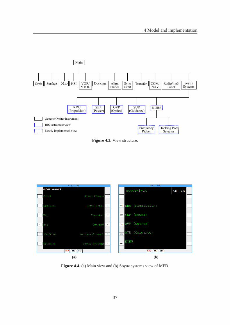
4 Model and implementation
Main
Orbit Surface VOR/VTOL
Docking AlignPlanes
SyncOrbit
Transfer COM/NAV
Radio/mp3Panel
SoyuzSystems
KDU(Propulsion)
SEP(Power)
OVP(Optics)
SUD(Guidance)
KURS
FrequencyPicker
Docking PortSelector
HSI
Generic Orbiter instrument
IRS instrument/view
Newly implemented view
Figure 4.3.View structure.
(a) (b)
Figure 4.4.(a) Main view and (b) Soyuz systems view of MFD.
37

4 Model and implementation
(a) (b)
Figure 4.5.(a) Off display and (b) long test display of KURS.
is to turn it off using the “OFF” button. Otherwise, no data isdisplayed. An example isshown in figure4.5b.
SEARCH. While the KURS model is in “SEARCH” mode, the user can see thecurrentfrequency of the navigation device and how good the reception of the signal is. The greenbar visualizes the received signal strength. If it is above the yellow line, the vehicle is inrange of the transmitter. In case the pilot needs to tune the navigation device to a differentfrequency, he can press the “FRQ” button in order to reach thefrequency picker subviewdepicted in figure4.6b. In this view, the current frequency and channel number of thevehicle’s navigation device are displayed. In the Orbiter simulator, each navigation devicehas channels ranging from0 to 639. To convert a channel numberch into a frequency,use [11]
f = (108.0 + 0.05 ch) MHz. (4.2)
The buttons on the left and right can be used to change the channel number and thereforealso the frequency. “+++” increases the channel number by100, “++” by 10, and “+” by1. The buttons on the left decrease the channel number by the respective amount. Oncethe desired frequency has been reached, the pilot can use the“<–” button to return to theprevious (in this case: search) view.
SNC. In the “SNC” mode, the display is very similar to the one before in the “SEARCH”mode (see figure4.7a). The current frequency is shown as well as a bar indicating thereceived signal strength. Likewise, there is a “FRQ” buttonon the right in case the fre-quency needs to be changed. Additionally, the pilot now can also monitor the current lineof sight pitch and yaw angles. Note that during the SNC mode, the vehicle is aligningwith the line of sight and therefore, the pitch and yaw anglesshould decrease to zero ifthe KURS model is working properly.
LOCK-ON . During “LOCK-ON”, even more flight data is available to the pilot: In ad-dition to the previous information (frequency, signal strength, LOS pitch and yaw), now
38

4 Model and implementation
(a) (b)
Figure 4.6.(a) Search display and (b) Frequency picker subview of KURS.
also the values for the LOS pitch and yaw rates are available,as well as the range and therange rate. Just as before, the frequency can be adjusted by pressing the “FRQ” button onthe right. An example lock-on display is shown in figure4.7b.
SHORT TEST. As the pilot cannot interact with the KURS system while it isperformingthe short system test (except to turn it off), the display looks exactly as during the longtest at the beginning.
APPROACH. The information available during the “APPROACH” mode is only slightlydifferent from the “LOCK-ON” mode (see figure4.8a). There are only two differences:First, only the LOS rates are available now, but not the actual values (which should bevery small anyway). Second, there is an additional button onthe right labelled “TGT”.This button leads the docking port selector. Here, all docking port numbers and their cor-responding IDS signal frequency of the target vessel are displayed. Figure4.8bshows alist of the available docking ports of the ISS and figure4.9shows a screenshot of the im-plemented ISS model with the respective docking ports. Withthe “up” and “dwn” buttonson the right, the pilot can switch between ports. The “SEL” button on the left selects theport currently displayed in yellow. Upon selection, the view automatically switches to thenext display of the KURS view. The docking port selection canbe performed any timeduring the approach, even before the station keeping position is acquired. The Soyuz willthen immediately start the flyaround.
FLYAROUND . While the vehicle is performing the flyaround to the selected dockingport, the pilot can monitor the line of sight angles, which now also inlcude the measure-ment of the roll misalignment. Note that now the line of sighthas changed and extendsfrom the Soyuz docking port to the selected docking port on the station. Additionally,the bearing angles are displayed. These are the LOS angles asseen from the station. Inother words, the LOS angles measured by Soyuz represent the orientation of the vehiclein reference to the selected station docking port, whereas the bearing angles represent thetranslational position with respect to the latter. Just like before, the range and range rate
39

4 Model and implementation
(a) (b)
Figure 4.7.(a) SNC display and (b) lock-on display of KURS.
(a) (b)
Figure 4.8.(a) Approach display and (b) docking port subview of KURS.
40

4 Model and implementation
1
2
3
Figure 4.9.Docking ports on the implemented ISS model.
are also displayed. As the vehicle is now fairly close to the station, there is no need todisplay the current frequency or received signal strength of the navigation device as theSoyuz should not be moving out of its range. Once the station keeping position in front ofthe docking port has been acquired, an additional line appears on the display saying “StartFINAL approach?”. Figure4.10ashows the display in this configuration. By pressing the“EXE” button, the pilot commands the Soyuz to start the final approach to the dockingport.
FINAL . During the final approach to the docking port, fewer relative motion parametersare available to the pilot than before (see figure4.10b). Only the roll misalignment isdisplayed, as well as the bearing angles, the range and rangerate. Additionally, the pilotreceives information about whether the 2AO antenna boom hasbeen retracted or not. Theretraction is usually takes place automatically. Note thatdocking with the antenna stilldeployed is prohibited. In the bottom of the display it now says “Abort FINAL approach?”.In case the pilot notices a malfunction, pressing the button“EXE” will abort the finalapproach and put the KURS system back into the “FLYAROUND” mode. In this way, themotion of the vehicle will be stopped and it will be directed to move back to the stationkeeping position at150m distance. The only other option for the pilot to interact with theKURS model at this point is to turn it off.
41

4 Model and implementation
(a) (b)
Figure 4.10.(a) Flyaround display and (b) Final approach display of KURS.
4.4 Procedures
In order to increase the authenticity of the IRS Soyuz simulator, flight procedures aredeveloped for the modelled systems. The procedure are used in reality to guide the astro-nauts through the many highly complex systems of the Soyuz spacecraft. In the simulator,so far no procedures are available to the students. Within the present thesis, an existingprocedures draft was enhanced and especially the procedures for an instrument basedrendezvous were developed. The simulator procedures try toreproduce the actual onesas close to reality as possible. However, procedures alwaysneed to be adapted to thosesystems, that the training pilot is actually working with. Including many items in the pro-cedures that do not exist in the simulator only confuses the users and contradicts the pointof procedures in general, which is to help the pilot with the system usage. The developedsimulator procedures draft can be found on the DVD accompanying this thesis.
42

Chapter 5
Results: Comparison of reality andmodel
5.1 General remarks
This chapter provides a comparison of the implemented KURS model and the real Soyuzsystem. The comparison covers a variety of different aspects from the hardware modellingto the differences in the resulting rendezvous sequence up to the differences in the frontend, i.e. the MFD simulator views versus the Russian formats. Most of the differences canbe related back to the general idea that aerospace engineering students will be using the si-mulator, and not astronauts training for a real mission. This often leads to simplifications,but can result in some additional features as well, as described in the following.
One major issue, that is not implemented in the IRS simulatorin general, is system mal-functions. Of course, during real astronaut training, preparing for malfunctions is whatmost of the training is about. However, in the IRS simulator,the training is more aboutgetting to know the system in general, without worrying about malfunctions.
In addition, the present project only implemented that partof the automated docking pro-cess that is provided by the KURS radar system and takes placein proximity of the station.However, what is beyond the scope of this thesis is that part of the motion control systemcalculating and executing the required rendezvous and correction burns to get the Soyuzvehicle from its phasing orbit to the station. At this point of time, a fully automated ren-dezvous and docking is not yet possible. Only when the vehicle is within400m of thestation, the implemented motion control system takes over and docks the vehicle automa-tically. Approaching the station up to this distance so far has to be achieved manually.
43

5 Results: Comparison of reality and model
5.2 KURS antennas and electronics
In the design process of the hardware component models, not all components are modelledas separate objects in the implemented KURS system. First ofall, the different KURSantennas on the Soyuz vehicle are not each modelled as separate objects. Moreover, onlya single built-in navigation device of the Orbiter simulator is used. No differentiationis made between which antenna currently receives a signal ormeasures a relative motionparameter. Instead, the implemented model uses the built-in navigation device to receive asignal in general. Besides, as this received signal does notcontain any information aboutthe relative motion parameters, the latter are determined using built-in functions of theOrbiter API.
The modelling of the different KURS antennas on the Soyuz vehicle is omitted for severalreasons: As mentioned in chapter3.1, one principle of object-oriented programming is tocreate objects that resemble reality only as far as necessary. It is not the primary goalfor the aerospace students training in the simulator to learn about radio signalling, butabout the rendezvous flight path and the operation of a complex vehicle. One argumentsupporting the modelling of different antennas is that thiswould allow for the simulationof malfunctions of single antennas. However, as mentioned above, malfunctions are notpart of the IRS Soyuz simulator. Therefore, the modelling ofseparate KURS antennas andtheir respective received and transmitted signals was considered unnecessary.
In the real Soyuz, the radar system not only consists of several antennas, but also of aset of electronics (filter, receiver, transmitter, etc.). All these electronics were also notmodelled in the IRS simulator for very similar reasons as theimplementation of separateantennas was omitted. The implemented KURS system itself does not contain any othercomponents in general, but is treated as a single object thatmeasures/calculates most ofthe things on its own. Besides, the real KURS system consistsof two of these electronicssets for redundancy. So far, only one KURS model is implemented in the simulator as asecond system would only be interesting for simulating malfunctions. If this is desiredat a later point of time, a second KURS system can be implemented by creating anotherinstance of the KURS class and assigning one boolean parameter indicating which mo-del is currently in use and another boolean parameter indicating whether the model ismalfunctioning or not.
5.3 KURS operating modes and other software differences
In reality, the KURS system switches directly from the “LOCK-ON” mode to the “FINALAPPROACH” mode. The implemented KURS model has additional operating modes.The “APPROACH” and “FLYAROUND” modes were added at the end of“LOCK-on”and at the beginning of “FINAL APPROACH”. This decision was made for the sake ofconvenience in order to simplify the implementation of the different flight phases and thecorresponding displays.
The two test modes “LONG TEST” and “SHORT TEST” are basicallyimplemented as
44

5 Results: Comparison of reality and model
timers, where the KURS model just waits for a certain amount of time before proceedingwith its operation. In reality, during the long test, both KURS sets are tested and duringthe short test, the “hot” set is tested again. However, as mentioned above, only one KURSmodel was implemented and malfunctions are not implementedin general. For these re-asons the implemented model cannot check any parameters andjust has to “pause” for agiven time. Another possibility would have been to simply ignore these two test modes.Nevertheless, these test modes were still desired in the implementation in order to give thestudents a more realistic experience for example when thereis no KURS data availableduring the short test while being fairly close (15 km) to the station.
Another, if yet smaller, difference between the mode implementation of the model and thereal system occurs at the end of the “APPROACH” mode. In reality, the vehicle is alignedwith the station’s axis in its station keeping position. In the implementation however, thevehicle acquires the same position but is pointed to the station’s center of gravity. Thisis due to the limitations of the IRS motion control system implementation(its autopilot,respectively).
In reality, the rendezvous far phase begins atT0 with the onboard computer integrating theequations of motions to determine the current state vector of the vehicle. This integrationleads to some errors in the propagated vector later on, whichare corrected during the“LOCK-ON” phase using a Kalman filter. As the simulator does not propagate the statevector, but calculates it again every time step, there is no need to correct the state vector.Therefore, no Kalman filter model is implemented in the simulator.
5.4 Crew operations
Most of the differences in crew operations either result from the fact that aerospace en-gineering students will be operating the simulator (instead of real astronauts). Anothergreat deal of variations are a consequence of another, previous, difference (e.g. in the de-termination of the relative motion paramters). First, the differences in the crew actions aredescribed, later the MFD “views” are compared to the equivalent “formats”.
After the KURS system is started and tested, it will look for asignal from the station’sKURS antennas. In reality, the KURS antennas on the Soyuz aretuned to pre-set frequen-cies and the crew cannot change them. In the simulator, a frequency picker view has beenimplemented. This allows the crew to vary the frequency of the built-in navigation deviceof the vehicle. In this way, the students can get a better ideaof the operation of the radiosystem.
Later on, during the near phase of the rendezvous, the crew has to select a docking portin the simulator. In reality, the crew does not select the docking port, yet they do knowwhich port they are supposed to dock to. The actual selectionof the docking port is madeby ground control ([1]). However, to make the simulator students independent of groundcontrol, the docking port selection was implemented as a crew task.
45
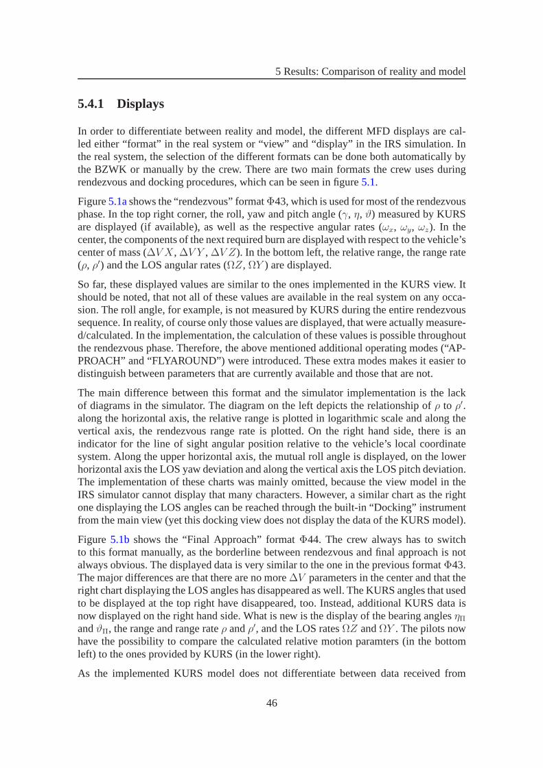
5 Results: Comparison of reality and model
5.4.1 Displays
In order to differentiate between reality and model, the different MFD displays are cal-led either “format” in the real system or “view” and “display” in the IRS simulation. Inthe real system, the selection of the different formats can be done both automatically bythe BZWK or manually by the crew. There are two main formats the crew uses duringrendezvous and docking procedures, which can be seen in figure5.1.
Figure5.1ashows the “rendezvous” formatF43, which is used for most of the rendezvousphase. In the top right corner, the roll, yaw and pitch angle (γ, η, ϑ) measured by KURSare displayed (if available), as well as the respective angular rates (ωx, ωy, ωz). In thecenter, the components of the next required burn are displayed with respect to the vehicle’scenter of mass (∆V X, ∆V Y , ∆V Z). In the bottom left, the relative range, the range rate(ρ, ρ′) and the LOS angular rates (ΩZ, ΩY ) are displayed.
So far, these displayed values are similar to the ones implemented in the KURS view. Itshould be noted, that not all of these values are available inthe real system on any occa-sion. The roll angle, for example, is not measured by KURS during the entire rendezvoussequence. In reality, of course only those values are displayed, that were actually measure-d/calculated. In the implementation, the calculation of these values is possible throughoutthe rendezvous phase. Therefore, the above mentioned additional operating modes (“AP-PROACH” and “FLYAROUND”) were introduced. These extra modes makes it easier todistinguish between parameters that are currently available and those that are not.
The main difference between this format and the simulator implementation is the lackof diagrams in the simulator. The diagram on the left depictsthe relationship ofρ to ρ′.along the horizontal axis, the relative range is plotted in logarithmic scale and along thevertical axis, the rendezvous range rate is plotted. On the right hand side, there is anindicator for the line of sight angular position relative tothe vehicle’s local coordinatesystem. Along the upper horizontal axis, the mutual roll angle is displayed, on the lowerhorizontal axis the LOS yaw deviation and along the verticalaxis the LOS pitch deviation.The implementation of these charts was mainly omitted, because the view model in theIRS simulator cannot display that many characters. However, a similar chart as the rightone displaying the LOS angles can be reached through the built-in “Docking” instrumentfrom the main view (yet this docking view does not display thedata of the KURS model).
Figure 5.1b shows the “Final Approach” formatF44. The crew always has to switchto this format manually, as the borderline between rendezvous and final approach is notalways obvious. The displayed data is very similar to the onein the previous formatF43.The major differences are that there are no more∆V parameters in the center and that theright chart displaying the LOS angles has disappeared as well. The KURS angles that usedto be displayed at the top right have disappeared, too. Instead, additional KURS data isnow displayed on the right hand side. What is new is the display of the bearing anglesηΠandϑΠ, the range and range rateρ andρ′, and the LOS ratesΩZ andΩY . The pilots nowhave the possibility to compare the calculated relative motion paramters (in the bottomleft) to the ones provided by KURS (in the lower right).
As the implemented KURS model does not differentiate between data received from
46

5 Results: Comparison of reality and model
(a) (b)
Figure 5.1.(a) FormatF43 “Rendezvous”; (b) formatF44 ”Final Approach“; both from [4].
KURS antennas and data calculated by the onboard computer, there is no need to dis-play the range, the range rate and the LOS angular rates twicein the simulator.
47
Chapter 6
Summary, conclusions and outlook
6.1 Summary and conclusions
The goal of this thesis was to implement a realistic model of the Soyuz spacecraft’s radarand docking systems in the IRS Soyuz simulator. In order to obtain a deeper insight intothe real systems, the present study was carried out in collaboration with EAC/ESA, wherethe author spent four weeks at their facilities in Cologne.
When modelling real systems, it is always important to find a well-balanced solution toattain a simple, yet realistic implementation. Usually, the implementation starts off as arough representation of reality and gets more realistic andrefined over multiple develop-ment cycles. Very often, decisions have to be made on prioritizing some systems (or theircomponents) over others.
Within the present thesis, these decisions included for example the modelling of theKURS antennas. A separate class was initialized for the KURSsystem itself, but its singleantennas were not implemented as extra objects.
The IRS simulator holds an additional concept, which has to be kept in mind when de-veloping models. That is the fact that the simulator is not intended to train and prepareastronauts for an actual space mission. Instead, it aims at giving aerospace students anopportunity to get a first-hand impression of what flying a spacecraft feels like (exceptwithout microgravity, of course). In this way, the studentshave the possibility to receivea practical experience for example of the consequences of a diminishing drag while per-forming attitude control. In addition, they also get a deeper insight in orbital mechanicswhen performing rendezvous maneuvers.
Taking the above into account did not just result for examplein leaving out malfunctionsin order to keep the vehicle handling simple. Indeed, some extra features were added tothe implemented model for the training to-be engineers. It is possible in the IRS simulatorto select a docking port before performing the flyaround in proximity of the station. Inreality, the docking port is preselected by ground control.When choosing the desireddocking port in the simulator, not only the docking port number is displayed, but also
48

6 Summary, conclusions and outlook
its respective antenna frequency. In this way the students see and learn what is behindselecting a docking port: It means setting the vehicle’s navigational device to a specificfrequency. Following the received signal will then guide the spacecraft to the desireddocking port.
When it comes to developing the procedures, in general, the same issues are taken intoconsideration as when implementing the models. Of course, procedures can only be writ-ten for systems respresented in the simulator. In addition,it has to be ensured that all ofthe procedures are manageable by a single person. In reality, there is a crew of three, butin the simulator, the students usually practice one at a time.
6.2 Outlook
The implementation of such a highly complex system such as the radar and docking sy-stem (not even to mention the Soyuz vehicle in general) always leaves room for extensionsand improvements. The implementation model could be refinedwith regards to modellingeach antenna individually or implementing two seperate electronics sets. In general, thesekind of enhancements will be most interesting if they also involve the implementation ofmalfunctions.
One option would also be to implement a model of the onboard computer including itsstate vector propagation. This propagation could be implemented in the simulator as anactual integration of the state vector. Another (maybe simpler) approach would be to mo-del the propagation by taking the actual correct state vector and randomly tamper with thevalues to simulate the integration errors. Thus, the relative motion parameters providedfrom the onboard computer would differ from those provided by the KURS model. In thisway, the importance of a Kalman filter could be demonstrated to the students. The Kalmanfilter itself can be implmented as an algorithm slowly decreasing the scope of how muchthe correct state vector is tempered with.
An additional feature would be procedures concerning the mechanical docking. Eventhough the single steps of the mechanical docking process cannot be implemented in thesimulator due to software restrictions, the leak checks following the docking, for example,could be modelled and included in the procedures.
In order to be able to perform a fully automated docking, the motion control system andits onboard computer need to be expanded. So far, the rendezvous burns have to be per-formed manually or can are pre-set in the scenario file. For anautomated docking, themotion control system needs to determine the desired interception point and the resul-ting maneuver time to meet up with the station. The maneuver time is the time the ISSneeds from the maneuver starting point to the interception point. From there, the resultingtransfer orbits of the bi-elliptic transfer can be calculated.
Finally, special KURS training scenarios should be developed for the Soyuz Rendezvousand Docking Seminar. This would offer the students trainingenvironments, in which they
49

6 Summary, conclusions and outlook
can get to know the KURS system and its operating modes, as well as familiarize themsel-ves with the according procedures. Within the present thesis, only one exemplary scenariowas developed to demonstrated the full capabilities of the KURS system. However, thedevelopment of such scenarios ranging from the orbit insertion to docking is complicated,as so far there is no automated calculation of the required main engine burns.
50

References
[1] D. Churkin. Personal communication, 2013. Astronaut Training Division, EAC/E-SA.
[2] S. Fasoulas. Personal communication, 2013. Professor at Space Systems Institute.
[3] A. Fink and M. Schmitz. Soyuz rendevous and docking simulator training. Univer-sity Lecture Notes, 2013. University of Stuttgart.
[4] Gagarin Russian State Scientific Research Testing Center for Cosmonaut Training.Soyuz TMA Crew Operations Manual, 2006.
[5] J. Liberty. Teach Yourself C++ in 21 days. Sams Publishing, Indianapolis, Indiana,2001.
[6] D. Louis. C/C++ Die praktische Referenz. Markt+Technik Verlag, Munich, Germa-ny, 2007.
[7] M. Schmitz. RTT Wiki -> Soyuz Simulator. URLhttp://phobos.irs.uni-stuttgart.de/~wiki/mediawiki/index.php5/Simulator.
[8] M. Schmitz. A simpit framework based on the orbiter spacesimulator and imple-mentation of a soyuz-style simpit. Studienarbeit, 2010. Sapce Systems Institute,University of Stuttgart.
[9] M. Schweiger. Orbiter Scenario Editor. Orbiter 2010 Edition SDK, 2006.
[10] M. Schweiger. Orbiter Programmer’s Guide. Orbiter 2010 Edition SDK, 2009.
[11] M. Schweiger. Orbiter API Reference Manual. Orbiter 2010 Edition SDK, 2010.
[12] M. Schweiger. Orbiter User Manual Spaceflight Simulator. Orbiter 2010 EditionSDK, 2010.
[13] M. Schweiger. Orbiter Spaceflight Simulator, July 2013. URL http://orbit.medphys.ucl.ac.uk/index.html.
51