modelling of slaughterhouse solid waste anaerobic digestion: determination of parameters and...

Waste Management 30 (2010) 1813–1821

Contents lists available at ScienceDirect

Waste Management

journal homepage: www.elsevier .com/locate /wasman

Modelling of slaughterhouse solid waste anaerobic digestion: Determinationof parameters and continuous reactor simulation

Iván López *, Liliana BorzacconiEngineering Faculty, Universidad de la República, J.Herrera y Reissig 565, Montevideo, Uruguay

a r t i c l e i n f o a b s t r a c t

Article history:Received 12 August 2009Accepted 26 February 2010Available online 19 March 2010

0956-053X/$ - see front matter � 2010 Elsevier Ltd. Adoi:10.1016/j.wasman.2010.02.034

* Corresponding author.E-mail address: [email protected] (I. López).

A model based on the work of Angelidaki et al. (1993) was applied to simulate the anaerobic biodegra-dation of ruminal contents. In this study, two fractions of solids with different biodegradation rates wereconsidered. A first-order kinetic was used for the easily biodegradable fraction and a kinetic expressionthat is function of the extracellular enzyme concentration was used for the slowly biodegradable fraction.Batch experiments were performed to obtain an accumulated methane curve that was then used toobtain the model parameters. For this determination, a methodology derived from the ‘‘multiple-shoot-ing” method was successfully used. Monte Carlo simulations allowed a confidence range to be obtainedfor each parameter. Simulations of a continuous reactor were performed using the optimal set of modelparameters. The final steady-states were determined as functions of the operational conditions (solidsload and residence time). The simulations showed that methane flow peaked at a flow rate of0:5—0:8 Nm3=d=m3

reactor at a residence time of 10–20 days. Simulations allow the adequate selection ofoperating conditions of a continuous reactor.

� 2010 Elsevier Ltd. All rights reserved.

1. Introduction

Anaerobic digestion is a widely used technology for organicwaste treatment. This is an option consistent with cleaner produc-tion and sustainable development due to the positive energy bal-ance for the waste treatment (no energy is input, and capturedbiogas is an energy source), the lowered production of sludgewaste and the fact that the sludge thus produced has a higher de-gree of stabilisation. Also, solids coming from the anaerobic stabi-lisation process can be used as soil-improving biosolids. In general,full-scale applications have been developed for the treatment of or-ganic solid waste, cattle manure or sewage sludge, either sepa-rately or in co-digestion (Mata-Alvarez et al., 2000; Salminen andRintala, 2002).

Wastes generated in slaughterhouses are of a peculiar nature,particularly the ruminal content, which contains a significantamount of partially digested lignocellulosic material (grass, straw,etc.). The lignocellulosic material forms a mesh that traps the bio-gas bubbles, and it therefore has a tendency to float in an anaerobicenvironment. As a result, conventional mixing systems can be inef-fective. Good mixing is a key to achieving a good substrate transferto microorganisms, and therefore, achieving optimum mixing is al-ways necessary to improve full-scale digester performance.

ll rights reserved.

Ammonia inhibition must also be controlled (Hansen et al.,1998; Wang and Banks, 2003; Güngör-Demirci and Demirer,2004). Ammonia exists in two forms in solution, ammonium ionand free unionised ammonia, with the unionised species havingthe higher inhibitory power, where the relative amounts of thesespecies depend on the pH of the medium. Inhibitory levels of 50–150 mg/L of free ammonia have been reported (Kayhanian, 1999;Eldem et al., 2004); however, methanogens may adapt to ammoniaconcentrations of several times the initial threshold level (Salmi-nen and Rintala, 2002).

Taking into account the complexity of the involved processes, itis useful to have simulation tools for guidance on the generalbehaviour of the digester prior to experimental or design stages.For this purpose, we took the kinetic model proposed by Angelidakiet al. (1993), also tested by other authors (Keshtkar et al., 2003), forsubstrates that are relatively similar to rumen content. This modelpays special attention to the ammonium inhibition phenomenon.In a complex substrate as the ruminal content, fractions with dif-ferent biodegradability rates are found (Myint et al., 2007). In thepresent work, the model was adapted to take into considerationthe presence of fractions with different degradation rates. A meth-od for the determination of model parameters, which derives fromthe ‘‘multiple-shooting” technique (Müller et al., 2002; Müller andTimmer, 2004; Kutalik et al., 2004), was proposed. Finally, simula-tion tests were performed using the kinetic model applied to a con-tinuous digester.

http://dx.doi.org/10.1016/j.wasman.2010.02.034

mailto:[email protected]

http://dx.doi.org/10.1016/j.wasman.2010.02.034

http://www.sciencedirect.com/science/journal/0956053X

http://www.elsevier.com/locate/wasman

1814 I. López, L. Borzacconi / Waste Management 30 (2010) 1813–1821

2. Materials and methods

2.1. The degradation model

The assumptions of the Angelidaki et al. (1993) model were ta-ken as the basis for the degradation model. Particular attention tothe enzymatic hydrolysis of solid material and the generation andconsumption of ammonium were taken into account in this model.In the present work, the following changes were made from thebase case: solid substrates with different degradabilities and differ-ent degradation rates were considered, and a more complex hydro-lysis rate, depending on the concentrations of extracellularenzymes, was used.

In anaerobic digestion, cellulosic solid material, represented as(C6H10O5�nNH3)ins, is first hydrolysed using extracellular enzymesto yield a soluble substrate (C6H10O5)sol, an inert fraction(C6H10O5�mNH3)inert and ammonia, as follows:

ðC6H10O5 � nNH3Þins ! YeðC6H10O5Þsol þ ð1� YeÞðC6H10O5

�mNH3Þinert þ ðn� ð1� YeÞmÞNH3 ð1Þ

where Ye represents the yield factor of the enzymes and n and m arethe insoluble and inert nitrogen content, respectively. Then, accord-ing to Angelidaki et al. (1993) the soluble substrate is degraded toorganic acids, producing biomass (C5H7NO2):

ðC6H10O5Þsol þ 0:1115NH3

! 0:1115C5H7NO2 þ 0:744CH3COOHþ 0:5CH3CH2COOHþ 0:4409CH3CH2CH2COOHþ 0:6909CO2 þ 0:0254H2O ð2Þ

Assuming a sufficiently rapid rate of hydrogen consumption (asassumed by Angelidaki et al. 1993), propionate and butyrate aredegraded in the acetogenesis step as follows:

CH3CH2COOHþ 0:06198NH3 þ 0:314H2O

! 0:06198C5H7NO2 þ 0:9345CH3COOHþ 0:6604CH4

þ 0:1607CO2 ð3Þ

CH3CH2CH2COOHþ 0:0653NH3 þ 0:5543CO2 þ 0:8038H2O

! 0:0653C5H7NO2 þ 1:8909CH3COOHþ 0:4452CH4 ð4Þ

Finally, the aceticlastic step is completed:

CH3COOHþ 0:022NH3 ! 0:022C5H7NO2 þ 0:945CH4 þ 0:945CO2

þ 0:066H2O ð5Þ

We considered two insoluble substrate fractions: a minor frac-tion that is easily hydrolysed and a major fraction (with high con-tent of lignocellulosic material) that is slowly hydrolysed. For theeasily hydrolysed substrate, a first-order kinetic rate expressionhas been proposed (Eastman and Ferguson, 1981):

rh ¼ khCins ð6Þ

with rh as the hydrolysis rate, kh as the hydrolysis constant and Cins

as the insoluble concentration. According to Angelidaki et al. (1993),volatile fatty acid (VFA) inhibition was considered in the form

kh ¼ khoKi

Ki þP

VFAð7Þ

where kho is a constant, Ki is the inhibition constant and VFA is thetotal VFA concentration (acetic, propionic and butyric acids in thismodel).

Assuming that, for the more slowly degradable fraction, theextracellular enzyme attack is a critical factor, a linear dependenceon enzyme concentration (Ce) was included in the hydrolysis con-stant for this fraction. The same VFA inhibition factor is considered.

kh2 ¼ kho2CeKi

Ki þP

VFAð8Þ

The enzyme-generation rate (re) is a function of the acidogenicbiomass concentration (Xa), of the substrate–biomass ratio (Cins/Xa)and also the enzyme concentration (Ce):

re ¼ keXaCins=Xa

K1si þ Cins=Xa

� �Ce

Kie þ Ce

� �ð9Þ

where ke is a constant; the first parenthetical term was proposed tointroduce into the model that enzyme production is by bacteriagrowing on the substrate surface (Myint et al., 2007) and the secondwas introduced to take into account enzymatic saturation.

Acidogenic biomass growth (la) was modelled with a Monodkinetic expression:

la ¼ lmaCs

Ksa þ Csð10Þ

where lma is the maximum growth rate of acidogenic microorgan-isms, Cs is the soluble substrate concentration and Ksa the semi-sat-uration constant. For the propionic and butyric degradation steps,we assumed a Monod kinetic rate affected by a non-competitiveinhibition term and a pH modulation factor (f(pH)):

lPr;But ¼ lm Pr;ButCPr;But

Ks Pr;But þ CPr;But

Ki

Ki þ Cacf ðpHÞ ð11Þ

where lm_Pr,But is the maximum growth rate for propionate- orbutyrate-degraders, respectively, Cac is the acetate concentration,CPr,But is the propionate or butyrate concentration, respectively,and Ks_Pr,But is the semi-saturation constant.

f ðpHÞ ¼ 1þ 2� 100:5ðpKl�pKhÞ

1þ 10ðpH�pKhÞ þ 10ðpKl�pHÞ ð12Þ

where pKl and pKh are lowest and highest pH values, respectively,that reduce the growth rate to the half-maximum value.

Finally, the aceticlastic step was also modelled as a Monod ki-netic rate with an ammonia inhibition factor and the same pHfactor:

lm ¼ lmmCac

Ksm þ Cac

Ki

Ki þ Camf ðpHÞ ð13Þ

where lmm is the maximum growth rate for methanogens, Ksm is thesemi-saturation constant and Cam is the ammonia concentration.The pH is determined using the ionic balance:

Hþ þ NHþ4 ¼ OH� þ Ac� þ Pr� þ Bu� þHCO�3 þ 2CO2�3 þ Z ð14Þ

where Z is the net ionic contribution (anions minus cations), as-sumed to be constant.

2.2. Determination of parameters

The proposed model must be able to take into account the exis-tence of substrate fractions with different degradabilities and di-verse kinetics. Thus, the following are needed for implementationof the model: (i) determination of the hydrolysis parameters, and(ii) the specific maximum growth rate for the involved popula-tions. Generalised parameters, or parameters less sensitive to envi-ronmental conditions, were taken from Angelidaki et al. (1993);thus, the remaining parameters to be determined from experimen-tal data are kho1, kho2, ke, K1si, Kie, lam and lmm.

Batch tests can be performed in order to easily estimate themodel parameters, and methane production can be monitored overtime. However, the process of parameters determination fromexperimental data is a complex task when the model is non-linearand the number of parameters is relatively high. Newton-basedmethods imply the knowledge or estimation of gradients, generally

I. López, L. Borzacconi / Waste Management 30 (2010) 1813–1821 1815

a virtually impossible objective due to non-linear characteristics.Direct-search methods, such as Simplex, work well for local opti-mum determination, but the high number of parameters makesthe global optimum determination a very difficult task. Other strat-egies, such as Genetic Algorithms or Simulated Annealing, are ex-tremely complex and often require abundant experimental data.

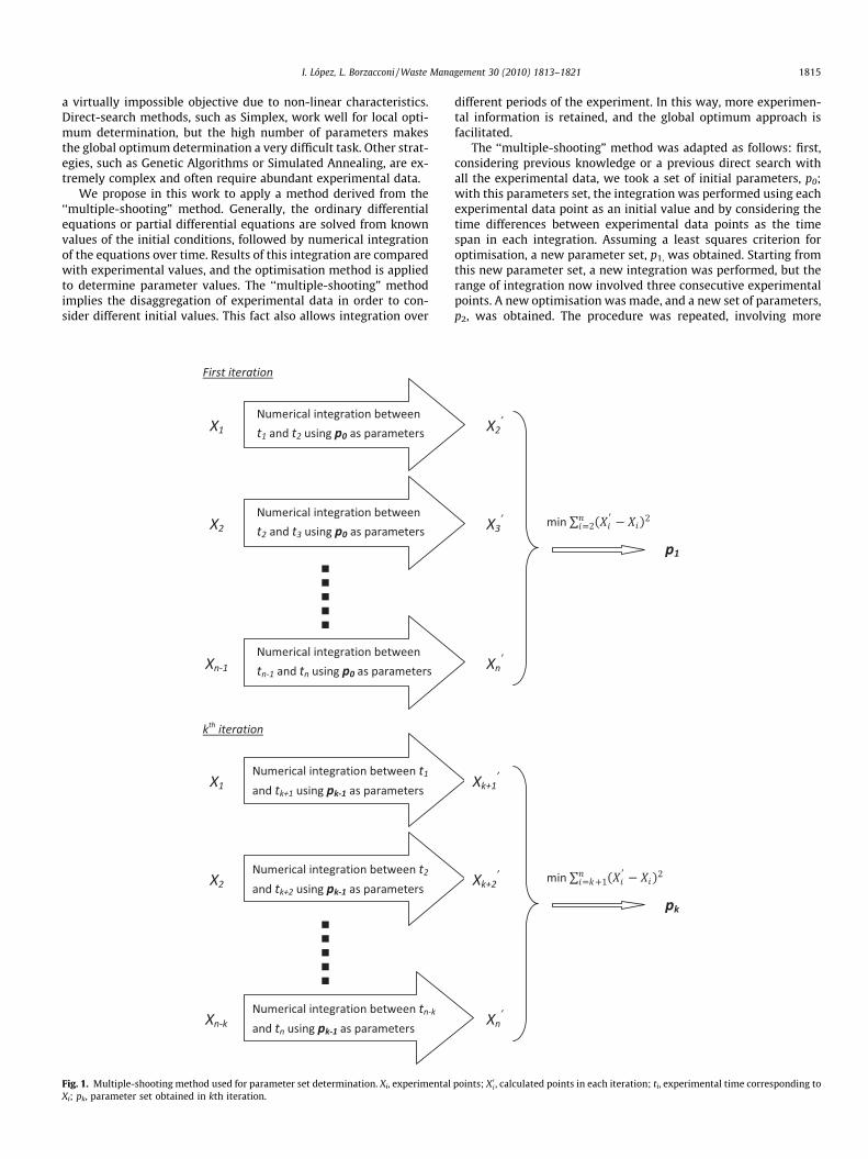
We propose in this work to apply a method derived from the‘‘multiple-shooting” method. Generally, the ordinary differentialequations or partial differential equations are solved from knownvalues of the initial conditions, followed by numerical integrationof the equations over time. Results of this integration are comparedwith experimental values, and the optimisation method is appliedto determine parameter values. The ‘‘multiple-shooting” methodimplies the disaggregation of experimental data in order to con-sider different initial values. This fact also allows integration over

Fig. 1. Multiple-shooting method used for parameter set determination. Xi, experimentalXi; pk, parameter set obtained in kth iteration.

different periods of the experiment. In this way, more experimen-tal information is retained, and the global optimum approach isfacilitated.

The ‘‘multiple-shooting” method was adapted as follows: first,considering previous knowledge or a previous direct search withall the experimental data, we took a set of initial parameters, p0;with this parameters set, the integration was performed using eachexperimental data point as an initial value and by considering thetime differences between experimental data points as the timespan in each integration. Assuming a least squares criterion foroptimisation, a new parameter set, p1, was obtained. Starting fromthis new parameter set, a new integration was performed, but therange of integration now involved three consecutive experimentalpoints. A new optimisation was made, and a new set of parameters,p2, was obtained. The procedure was repeated, involving more

points; X 0i , calculated points in each iteration; ti, experimental time corresponding to

3


experimental points each time. After n � 1 iterations (n + 1 is thenumber of experimental data points), the parameter set, pn, canbe considered to be the final result (Fig. 1).

0 10 20 30 40 50 60 70 80 900

0.5

1

1.5

2

2.5

time (d)

mm

ol C

H4

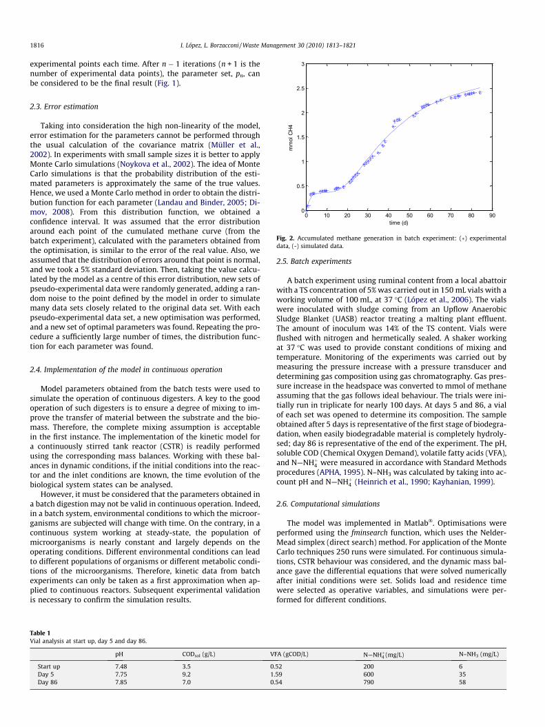
Fig. 2. Accumulated methane generation in batch experiment: (�) experimentaldata, (-) simulated data.

2.3. Error estimation

Taking into consideration the high non-linearity of the model,error estimation for the parameters cannot be performed throughthe usual calculation of the covariance matrix (Müller et al.,2002). In experiments with small sample sizes it is better to applyMonte Carlo simulations (Noykova et al., 2002). The idea of MonteCarlo simulations is that the probability distribution of the esti-mated parameters is approximately the same of the true values.Hence, we used a Monte Carlo method in order to obtain the distri-bution function for each parameter (Landau and Binder, 2005; Di-mov, 2008). From this distribution function, we obtained aconfidence interval. It was assumed that the error distributionaround each point of the cumulated methane curve (from thebatch experiment), calculated with the parameters obtained fromthe optimisation, is similar to the error of the real value. Also, weassumed that the distribution of errors around that point is normal,and we took a 5% standard deviation. Then, taking the value calcu-lated by the model as a centre of this error distribution, new sets ofpseudo-experimental data were randomly generated, adding a ran-dom noise to the point defined by the model in order to simulatemany data sets closely related to the original data set. With eachpseudo-experimental data set, a new optimisation was performed,and a new set of optimal parameters was found. Repeating the pro-cedure a sufficiently large number of times, the distribution func-tion for each parameter was found.

2.4. Implementation of the model in continuous operation

Model parameters obtained from the batch tests were used tosimulate the operation of continuous digesters. A key to the goodoperation of such digesters is to ensure a degree of mixing to im-prove the transfer of material between the substrate and the bio-mass. Therefore, the complete mixing assumption is acceptablein the first instance. The implementation of the kinetic model fora continuously stirred tank reactor (CSTR) is readily performedusing the corresponding mass balances. Working with these bal-ances in dynamic conditions, if the initial conditions into the reac-tor and the inlet conditions are known, the time evolution of thebiological system states can be analysed.

However, it must be considered that the parameters obtained ina batch digestion may not be valid in continuous operation. Indeed,in a batch system, environmental conditions to which the microor-ganisms are subjected will change with time. On the contrary, in acontinuous system working at steady-state, the population ofmicroorganisms is nearly constant and largely depends on theoperating conditions. Different environmental conditions can leadto different populations of organisms or different metabolic condi-tions of the microorganisms. Therefore, kinetic data from batchexperiments can only be taken as a first approximation when ap-plied to continuous reactors. Subsequent experimental validationis necessary to confirm the simulation results.

Table 1Vial analysis at start up, day 5 and day 86.

pH CODsol (g/L) V

Start up 7.48 3.5 0.Day 5 7.75 9.2 1.Day 86 7.85 7.0 0.

2.5. Batch experiments

A batch experiment using ruminal content from a local abattoirwith a TS concentration of 5% was carried out in 150 mL vials with aworking volume of 100 mL, at 37 �C (López et al., 2006). The vialswere inoculated with sludge coming from an Upflow AnaerobicSludge Blanket (UASB) reactor treating a malting plant effluent.The amount of inoculum was 14% of the TS content. Vials wereflushed with nitrogen and hermetically sealed. A shaker workingat 37 �C was used to provide constant conditions of mixing andtemperature. Monitoring of the experiments was carried out bymeasuring the pressure increase with a pressure transducer anddetermining gas composition using gas chromatography. Gas pres-sure increase in the headspace was converted to mmol of methaneassuming that the gas follows ideal behaviour. The trials were ini-tially run in triplicate for nearly 100 days. At days 5 and 86, a vialof each set was opened to determine its composition. The sampleobtained after 5 days is representative of the first stage of biodegra-dation, when easily biodegradable material is completely hydroly-sed; day 86 is representative of the end of the experiment. The pH,soluble COD (Chemical Oxygen Demand), volatile fatty acids (VFA),and N—NHþ4 were measured in accordance with Standard Methodsprocedures (APHA, 1995). N–NH3 was calculated by taking into ac-count pH and N—NHþ4 (Heinrich et al., 1990; Kayhanian, 1999).

2.6. Computational simulations

The model was implemented in Matlab�. Optimisations wereperformed using the fminsearch function, which uses the Nelder-Mead simplex (direct search) method. For application of the MonteCarlo techniques 250 runs were simulated. For continuous simula-tions, CSTR behaviour was considered, and the dynamic mass bal-ance gave the differential equations that were solved numericallyafter initial conditions were set. Solids load and residence timewere selected as operative variables, and simulations were per-formed for different conditions.

FA (gCOD/L) N—NHþ4 (mg/L) N–NH3 (mg/L)

52 200 659 600 3554 790 58

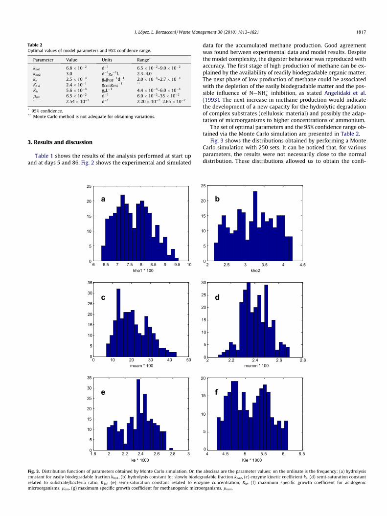
Table 2Optimal values of model parameters and 95% confidence range.

Parameter Value Units Range*

kho1 6.8 � 10�2 d�1 6.5 � 10�2–9.0 � 10�2

kho2 3.0 d�1ge�1L 2.3–4.0

ke 2.5 � 10�3 gegVSS�1d�1 2.0 � 10�3–2.7 � 10�3

K1si 2.4 � 10�1 gCODgVSS�1 **

Kie 5.6 � 10�3 geL�1 4.4 � 10�3–6.0 � 10�3

lam 6.5 � 10�2 d�1 6.0 � 10�2–35 � 10�2

‘ 2.54 � 10�2 d�1 2.20 � 10�2–2.65 � 10�2

* 95% confidence.** Monte Carlo method is not adequate for obtaining variations.


3. Results and discussion

Table 1 shows the results of the analysis performed at start upand at days 5 and 86. Fig. 2 shows the experimental and simulated

6 6.5 7 7.5 8 8.5 9 9.5 100

5

10

15

20

25

kho1 * 100

1

1

2

2

0 10 20 30 40 500

5

10

15

20

25

30

35

muam * 100

1.8 2 2.2 2.4 2.6 2.8 30

5

10

15

20

25

30

35

ke * 1000

1

1

2

a

c

e

Fig. 3. Distribution functions of parameters obtained by Monte Carlo simulation. On theconstant for easily biodegradable fraction kho1, (b) hydrolysis constant for slowly biodegrelated to substrate/bacteria ratio, K1si, (e) semi-saturation constant related to enzymicroorganisms, lam, (g) maximum specific growth coefficient for methanogenic microo

data for the accumulated methane production. Good agreementwas found between experimental data and model results. Despitethe model complexity, the digester behaviour was reproduced withaccuracy. The first stage of high production of methane can be ex-plained by the availability of readily biodegradable organic matter.The next phase of low production of methane could be associatedwith the depletion of the easily biodegradable matter and the pos-sible influence of N—NHþ4 inhibition, as stated Angelidaki et al.(1993). The next increase in methane production would indicatethe development of a new capacity for the hydrolytic degradationof complex substrates (cellulosic material) and possibly the adap-tation of microorganisms to higher concentrations of ammonium.

The set of optimal parameters and the 95% confidence range ob-tained via the Monte Carlo simulation are presented in Table 2.

Fig. 3 shows the distributions obtained by performing a MonteCarlo simulation with 250 sets. It can be noticed that, for variousparameters, the results were not necessarily close to the normaldistribution. These distributions allowed us to obtain the confi-

2 2.5 3 3.5 4 4.50

5

0

5

0

5

kho2

2 2.2 2.4 2.6 2.80

5

10

15

20

25

30

mumm * 100

4 4.5 5 5.5 6 6.50

5

0

5

0

Kie * 1000

b

d

f

abscissa are the parameter values; on the ordinate is the frequency; (a) hydrolysisradable fraction kho2, (c) enzyme kinetic coefficient ke, (d) semi-saturation constantme concentration, Kie, (f) maximum specific growth coefficient for acidogenicrganisms, lmm.

0 10 20 30 40 50 60 70 800

5

X (g

VS/L

)

0 10 20 30 40 50 60 70 800

50

100in

solu

ble

(gVS

/L)

0 10 20 30 40 50 60 70 800

2

4

solu

ble

CO

D (g

/L)

0 10 20 30 40 50 60 70 800

5

10

met

hane

flow

(Nm

3/d)

0 10 20 30 40 50 60 70 80

5

6

7

time (d)

pH

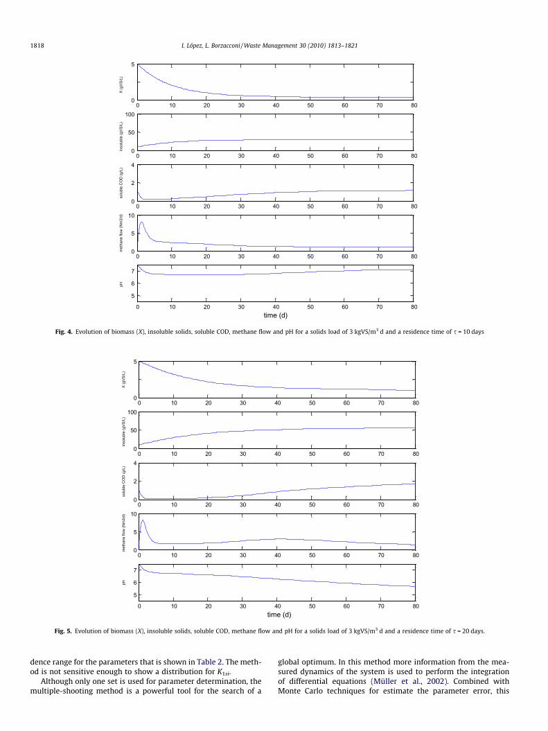
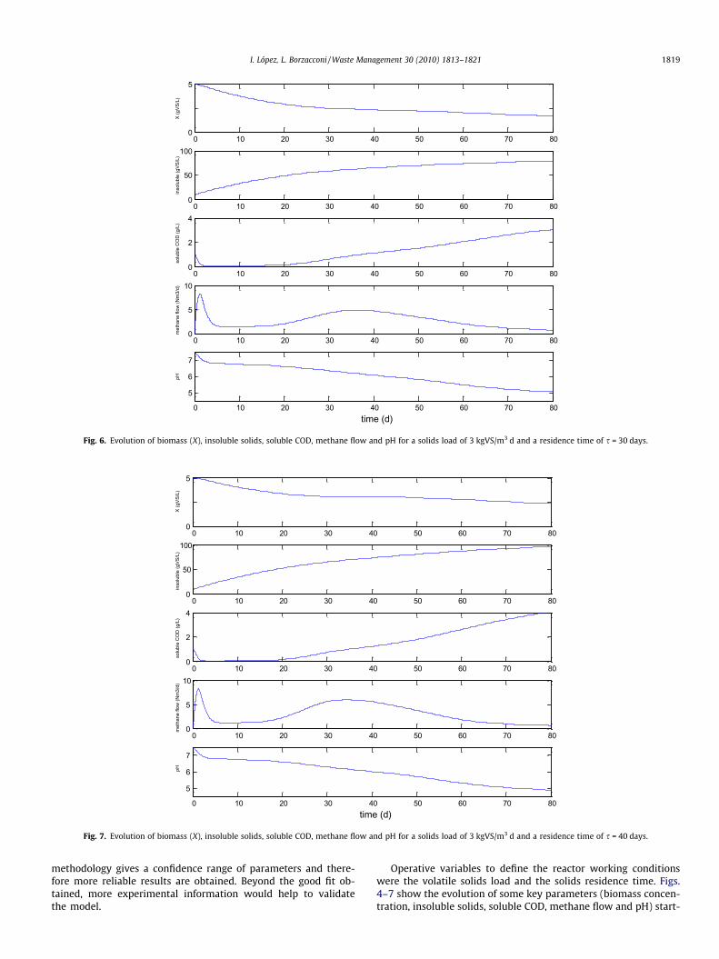
Fig. 4. Evolution of biomass (X), insoluble solids, soluble COD, methane flow and pH for a solids load of 3 kgVS/m3 d and a residence time of s = 10 days

0 10 20 30 40 50 60 70 800

5

X (g

VS/L

)

0 10 20 30 40 50 60 70 800

50

100

inso

lubl

e (g

VS/L

)

0 10 20 30 40 50 60 70 800

2

4

solu

ble

CO

D (g

/L)

0 10 20 30 40 50 60 70 800

5

10

met

hane

flow

(Nm

3/d)

0 10 20 30 40 50 60 70 80

5

6

7

time (d)

pH

Fig. 5. Evolution of biomass (X), insoluble solids, soluble COD, methane flow and pH for a solids load of 3 kgVS/m3 d and a residence time of s = 20 days.


dence range for the parameters that is shown in Table 2. The meth-od is not sensitive enough to show a distribution for K1si.

Although only one set is used for parameter determination, themultiple-shooting method is a powerful tool for the search of a

global optimum. In this method more information from the mea-sured dynamics of the system is used to perform the integrationof differential equations (Müller et al., 2002). Combined withMonte Carlo techniques for estimate the parameter error, this

0 10 20 30 40 50 60 70 800

5

X (g

VS/L

)

0 10 20 30 40 50 60 70 800

50

100

inso

lubl

e (g

VS/L

)

0 10 20 30 40 50 60 70 800

2

4

solu

ble

CO

D (g

/L)

0 10 20 30 40 50 60 70 800

5

10

met

hane

flow

(Nm

3/d)

0 10 20 30 40 50 60 70 80

5

6

7

time (d)

pH


0 10 20 30 40 50 60 70 800

5

X (g

VS/L

)

0 10 20 30 40 50 60 70 800

50

100

inso

lubl

e (g

VS/L

)

0 10 20 30 40 50 60 70 800

2

4

solu

ble

CO

D (g

/L)

0 10 20 30 40 50 60 70 800

5

10

met

hane

flow

(Nm

3/d)

0 10 20 30 40 50 60 70 80

5

6

7

time (d)

pH



methodology gives a confidence range of parameters and there-fore more reliable results are obtained. Beyond the good fit ob-tained, more experimental information would help to validatethe model.

Operative variables to define the reactor working conditionswere the volatile solids load and the solids residence time. Figs.4–7 show the evolution of some key parameters (biomass concen-tration, insoluble solids, soluble COD, methane flow and pH) start-

1020

3040

2

4

6

80

50

100

150

200

250

residence time (d)load (kgVS/m3/d)

inso

lubl

e (g

VS/L

)

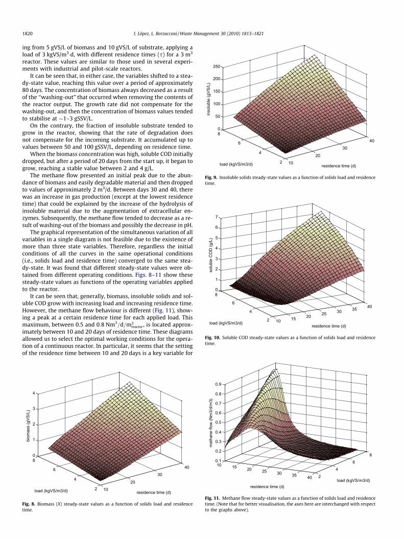
Fig. 9. Insoluble solids steady-state values as a function of solids load and residencetime.

10 15 20 25 30 35 40

2

4

6

80

1

2

3

4

5

6

7


solu

ble

CO

D (g

/L)

Fig. 10. Soluble COD steady-state values as a function of solids load and residencetime.


ing from 5 gVS/L of biomass and 10 gVS/L of substrate, applying aload of 3 kgVS/m3�d, with different residence times (s) for a 3 m3

reactor. These values are similar to those used in several experi-ments with industrial and pilot-scale reactors.

It can be seen that, in either case, the variables shifted to a stea-dy-state value, reaching this value over a period of approximately80 days. The concentration of biomass always decreased as a resultof the ‘‘washing-out” that occurred when removing the contents ofthe reactor output. The growth rate did not compensate for thewashing-out, and then the concentration of biomass values tendedto stabilise at �1–3 gSSV/L.

On the contrary, the fraction of insoluble substrate tended togrow in the reactor, showing that the rate of degradation doesnot compensate for the incoming substrate. It accumulated up tovalues between 50 and 100 gSSV/L, depending on residence time.

When the biomass concentration was high, soluble COD initiallydropped, but after a period of 20 days from the start up, it began togrow, reaching a stable value between 2 and 4 g/L.

The methane flow presented an initial peak due to the abun-dance of biomass and easily degradable material and then droppedto values of approximately 2 m3/d. Between days 30 and 40, therewas an increase in gas production (except at the lowest residencetime) that could be explained by the increase of the hydrolysis ofinsoluble material due to the augmentation of extracellular en-zymes. Subsequently, the methane flow tended to decrease as a re-sult of washing-out of the biomass and possibly the decrease in pH.

The graphical representation of the simultaneous variation of allvariables in a single diagram is not feasible due to the existence ofmore than three state variables. Therefore, regardless the initialconditions of all the curves in the same operational conditions(i.e., solids load and residence time) converged to the same stea-dy-state. It was found that different steady-state values were ob-tained from different operating conditions. Figs. 8–11 show thesesteady-state values as functions of the operating variables appliedto the reactor.

It can be seen that, generally, biomass, insoluble solids and sol-uble COD grow with increasing load and increasing residence time.However, the methane flow behaviour is different (Fig. 11), show-ing a peak at a certain residence time for each applied load. Thismaximum, between 0.5 and 0:8 Nm3=d=m3

reactor , is located approx-imately between 10 and 20 days of residence time. These diagramsallowed us to select the optimal working conditions for the opera-tion of a continuous reactor. In particular, it seems that the settingof the residence time between 10 and 20 days is a key variable for

1020

3040

2

4

6

80

1

2

3

4


biom

ass

(gVS

/L)

Fig. 8. Biomass (X) steady-state values as a function of solids load and residencetime.

10 15 20 25 30 35 40 24

68

0.1

0.2

0.3

0.4

0.5

0.6

0.7

0.8

0.9

load (kgVS/m3/d)residence time (d)

met

hane

flow

(Nm

3/d/

m3)

Fig. 11. Methane flow steady-state values as a function of solids load and residencetime. (Note that for better visualisation, the axes here are interchanged with respectto the graphs above).


optimising methane production, regardless of the values of theother variables.

These results agree with the performance of a 3.5 m3 pilot reac-tor treating ruminal content (López et al., 2006). In this pilot reac-tor a steady-state of 3.5 m3/d of biogas with 70% of methanecontent was obtained, with a solid retention time of 20 days and3–4% of solid content in the reactor.

4. Conclusions

Anaerobic biodegradation of slaughterhouse solid wastes is acomplex task. Previous models for solids anaerobic biodegradationmust be adapted to take into account two fractions with differentbiodegradability rates. A first-order kinetic was satisfactory to ex-plain the hydrolysis step for the easily biodegradable fraction, but,for the hydrolysis of the slowly biodegradable fraction, a kineticexpression that takes into consideration the extracellular enzymeconcentration was used. This combined expression better ex-plained the cumulated methane production curve obtainedthrough a batch test.

A strategy derived from the ‘‘multiple-shooting” method wasproposed to obtain the model parameters from a biodegradationbatch experiment. In this way, parameters added to the previousmodel and those that depend on the environmental conditionswere determined. The confidence range of those parameters wasestimated using a Monte Carlo technique. The results obtained per-forming this methodology are more reliable that other search typesbecause they use more information in the integration of differen-tial equations and because a estimation of the confidence rangeof parameters is found. Moreover, taking into account the goodfit obtained which reflects very satisfactorily the experimentaldata, the model can be used for simulations.

Once model parameters were determined, the model was ap-plied to simulate a continuous reactor, idealised as CSTR behaviour.Simulations showed the evolution of variables until steady-stateconditions were achieved after about 80 days. Steady-state pointsdepended on operative variables, including the solids load appliedand the retention time. An increase in the residence time or in thesolids load caused an increase in the biomass concentration, in theinsoluble solids concentration and in the soluble COD. The meth-ane flow showed a peak at around 10–20 days of residence time,the magnitude of which increased with the solids load. Optimisa-tion of reactor design can be performed using these simulations.Thus, the adequate selection of the residence time can be used to

in order to obtain a maximum biogas production or a maximumsolids removal rate. Simulations results are in agreement withexperiments performed with a continuous pilot reactor.

References

Angelidaki, I., Ellegaard, L., Ahring, B.K., 1993. A mathematical model for dynamicsimulation of anaerobic digestión of complex substrates: focusing on ammoniainhibition. Biotechnol. Bioeng. 42 (2), 159–166.

APHA, AWWA, WEF, 1995. Standard Methods for the Examination of Water andWastewater, 19th ed.

Dimov, I.T., 2008. Monte Carlo Methods for Applied Scientist, Ed. World Scientific.Eastman, J.A., Ferguson, J.F., 1981. Solubilization of particulate organic carbon

during the acid phase of anaerobic digestion. J. Water Pollut. Control Fed. 53,352–366.

Eldem, N.Ö., Ozturk, I., Soyer, E., Calli, B., Akgiray, Ö., 2004. Ammonia an pHinhibition in anaerobic treatment of wastewaters, Part I: experimental. J.Environ. Sci. Health – Part A-Toxic Hazard. Subst. Environ. Eng. A39 (9), 2405–2420.

Güngör-Demirci, G., Demirer, G.N., 2004. Effect of initial COD concentration,nutrient addition, temperature and microbial acclimatation on anaerobictreatability of broiler and cattle maure. Biores. Technol. 93, 109–117.

Hansen, K.H., Angelidaki, I., Ahring, B.K., 1998. Anaerobic digestion of swinemanure: inhibition by ammonia. Wat. Res. 32 (1), 5–12.

Heinrich, D.M., Poggi-Varaldo, H.M., Oleszkiewicz, J.O., 1990. Effects of ammonia onanaerobic digestion of simple organic substrates. J. Environ. Eng. ASCE 116 (4),698–710.

Kayhanian, M., 1999. Ammonia inhibition in high-solids biogasification: anoverview and practical solutions. Environ. Technol. 20 (4), 355–365.

Keshtkar, A., Meyssami, B., Abolhamd, G., Ghaforian, H., Khalagi Asadi, M., 2003.Mathematical modeling of non-ideal mixing continuous flow reactors foranaerobic digestion of cattle manure. Biores. Technol. 87, 113–124.

Kutalik, Z., Cho, K.-H., Wolkenhauer, O., 2004. Optimal sampling time selection forparameter estimation in dynamic pathway modeling. BioSystems 75, 43–55.

Landau, D.P., Binder, K., 2005. A Guide to Monte Carlo Simulations in StatisticalPhysics, second ed. Cambridge University Press.

López, I., Passeggi, M., Borzacconi, L., 2006. Co-digestion of ruminal content andblood from slaughterhouse industries – influence of solid concentration andammonium generation. Wat. Sci. Technol. 54 (2), 231–236.

Mata-Alvarez, J., Macé, S., Llabrés, P., 2000. Anaerobic digestion of organic solidwastes. An overview of research achievements and perspectives. Biores.Technol. 74, 3–16.

Müller, T.G., Noykova, N., Gyllenberg, M., Timmer, J., 2002. Parameter identificationin dynamical models of anaerobic waste water treatment. Math. Biosci. 177–178, 147–160.

Müller, T.G., Timmer, J., 2004. Parameter identification techniques for partialdifferential equations. Int. J. Bifurcat. Chaos 14 (6), 2053–2060.

Myint, M., Nirmalakhandan, N., Speece, R.E., 2007. Anaerobic fermentation of cattlemanure: modeling of hydrolysis and acidogenesis. Wat. Res. 41, 323–332.

Noykova, N., Müller, T.G., Gyllenberg, M., Timmer, J., 2002. Quantitative analyses ofanaerobic wastewater treatment processes: identifiability and parameterestimation. Biotechnol. Bioeng. 78 (1), 89–103.

Salminen, E., Rintala, J., 2002. Anaerobic digestion of organic solid poultryslaughterhouse waste – a review. Biores. Technol. 83, 13–26.

Wang, Z., Banks, Ch.J., 2003. Evaluation of a two stage anaerobic digester for thetreatment of mixed abattoir wastes. Process Biochem. 38, 1267–1273.

modelling of slaughterhouse solid waste anaerobic digestion: determination of parameters and...

Documents