modelling of hemicellulose degradation during softwood...
TRANSCRIPT

Modelling of Hemicellulose Degradation during
Softwood Kraft Pulping
Master of Science Thesis
JONAS WETTERLING
Department of Chemical and Biological Engineering
Division of Forest Products and Chemical Engineering
CHALMERS UNIVERSITY OF TECHNOLOGY
Gothenburg, Sweden, 2012


Modelling of Hemicellulose Degradation during Softwood Kraft Pulping
JONAS WETTERLING
Forest Products and Chemical Engineering
Department of Chemical and Biological Engineering
Chalmers University of Technology
Abstract Although kraft pulping has long been the predominantly used pulping process, models describing the
carbohydrate degradation during these conditions are insufficient. Focus has historically been on
describing the delignification whereas less attention has been paid to the hemicellulose degradation.
This thesis aim to provide models of the degradation and dissolution of the main softwood
hemicelluloses, glucomannan and xylan, while considering the distinctly different degradation
mechanisms involved. The models are based on an extensive set of experimental data generated
through laboratory cooking of Scots pine (Pinus sylvestris) wood meal in constant composition cooks.
The glucomannan loss can be accurately described by the degradation to monomers through endwise
degradation as well as alkaline hydrolysis, either through accounting for the cooking liquor
composition by power law expressions or by using equilibrium constants related to rate limiting
intermediates. The xylan removal is on the other hand largely controlled by the solubility of
polysaccharide fragments and may thus rather be described by a continuous distribution of reactivity
model.
As the glucomannan removal is controlled by the degradation, the cooking temperature and hydroxide
ion concentration had the largest impact on the overall yield. The degree of delignification seemed to
affect the extent of primary peeling obtained, possibly due to a physical stopping reaction of the
endwise degradation as a result of lignin-carbohydrate linkages. This effect was minor among the kraft
cooking experiments, although a significantly higher glucomannan yield is obtained during soda cook
experiments. The removal of xylan had a more pronounced correlation with delignification and thus
the hydrogen sulphide concentration. The retention of xylan is however decreased at higher ionic
strengths due to the decreased solubility of polysaccharide fragments.
Keywords: kraft cooking, hemicellulose, degradation, glucomannan, xylan, modelling, reaction
kinetics, equilibrium based model, continuous distribution of reactivity

Table of Contents 1. Introduction .............................................................................................................................. 1
1.2 Background ......................................................................................................................... 1
1.3 Aim .................................................................................................................................... 1
2. Theory ...................................................................................................................................... 2
2.1 Chemical composition of softwood ....................................................................................... 2
2.1.1 Cellulose ....................................................................................................................... 2
2.1.2 (Galacto)glucomannan ................................................................................................... 2
2.1.3 Arabinoglucuronoxylan.................................................................................................. 3
2.1.4 Lignin ........................................................................................................................... 4
2.2 Carbohydrate degradation reactions....................................................................................... 4
2.2.1 Mechanism of peeling reaction ....................................................................................... 6
2.2.2 Mechanism of alkaline hydrolysis ................................................................................... 8
2.3 Kinetic models for carbohydrate degradation ......................................................................... 9
2.3.1 Phase models................................................................................................................. 9
2.3.2 Reaction mechanism based models ................................................................................13
2.3.3 Continuous distribution of reactivity model ....................................................................16
3. Method ....................................................................................................................................18
3.1 Experimental methods .........................................................................................................18
3.2 Mathematical modelling methods.........................................................................................18
4. Results and discussion ..............................................................................................................20
4.1 Carbohydrate degradation and dissolution ............................................................................20
4.1.1 Effect of temperature ....................................................................................................20
4.1.2 Effect of hydroxide ion concentration ............................................................................21
4.1.3 Effect of hydrogen sulphide concentration......................................................................23
4.1.4 Effect of ionic strength..................................................................................................26
4.2 Modelling of glucomannan degradation................................................................................27
4.2.1 Wigell model................................................................................................................27
4.2.2 Equilibrium based model...............................................................................................31
4.3 Modelling of xylan removal.................................................................................................39
4.3.1 Phase model .................................................................................................................39
4.3.2 Continuous distribution of reactivity model ....................................................................43
4.4 Validation of glucomannan models ......................................................................................47
4.4.1 Validation using soda cooking experiments ....................................................................47
4.4.2 Validation using ionic strength experiments ...................................................................50
4.4.3 Validation using experiments with lower cooking temperatures .......................................51

4.4.4 Validation at lower liquor to wood ratio .........................................................................54
4.4.5 Validation with sodium borohydride addition .................................................................57
4.5 Validation of xylan models ..................................................................................................58
4.5.1 Validation using ionic strength experiments ...................................................................59
4.5.2 Validation using experiments with lower cooking temperatures .......................................61
4.5.3 Validation at lower liquor to wood ratio .........................................................................63
5. Conclusions .............................................................................................................................66
Acknowledgements ......................................................................................................................67
References ...................................................................................................................................68

1
1. Introduction
1.2 Background
The pulp and paper industry has a long tradition in Sweden. The pulp is produced by liberating the
wood fibres in the raw material, either mechanically through shear forces or by dissolving the lignin
fraction through chemical treatment. Mechanical pulping is an energy demanding process resulting in
a good material efficiency due to the high yields obtained whereas chemical pulping typically has
yields of about 50 %. The effective recovery of cooking chemicals in the kraft process, as well as the
high pulp quality obtained, is however the reason that kraft pulping is the predominant method for
pulp production.
The kraft process produces pulp by the cooking of wood chips in alkaline liquor containing hydrogen
sulphide. Cooking chemicals are then recovered and recirculated whereas the dissolved wood material
is used for energy production. Lignin is however not the only wood component that is degraded during
the alkaline cooking conditions as substantial losses of carbohydrates accompany the lignin removal.
The produced pulp has very high cellulose content whereas most of the hemicelluloses and lignin has
been degraded and dissolved. Although increasing the hemicellulose yield would have a positive
impact on the profitability of pulping process, sufficient knowledge regarding many features of the
process is still lacking. This shows the complexity of this over century old process.
The focus of this study is on the reaction kinetics of the main hemicelluloses in softwood, namely
glucomannan and xylan. The degradation mechanisms are studied in order to formulate models for the
hemicellulose removal during kraft pulping conditions. An extensive set of experimental data
concerning the carbohydrate composition after laboratory cooking will be used as the basis for the
modelling. The experimental data has been generated during studies on the delignification kinetics
carried out within the project Avancell - Centre for Fibre Engineering, but the carbohydrate
composition has previously not been studied further.
1.3 Aim
The objective of this thesis is to describe the degradation of glucomannan and xylan during kraft
cooking of softwood meal. The effect of temperature and cooking liquor composition concerning
hydroxide ion concentration, hydrogen sulphide ion concentration and total salt concentration (ionic
strength) are considered in the models. The modelling is focused at not only describing the observed
trends from the experimental data, but rather provide explanations for the studied behaviour in order to
be applicable over a wider range of cooking conditions.

2
2. Theory This chapter gives a brief description of the chemical components present in wood. It also presents the
most important carbohydrate degradation reactions along with the corresponding reaction
mechanisms. Existing models for carbohydrate removal during chemical pulping are also presented
along with a brief discussion about the reasoning behind the various approaches to modelling that has
been taken.
2.1 Chemical composition of softwood
Wood is a material mainly built of fibres. These long and slender fibre cells are called tracheids and
constitute 90-95 % of the cells. The fibres give softwood mechanical strength and allow for water
transport. The cell walls are mainly composed of cellulose, hemicellulose and lignin. Cellulose can be
seen as the basis for the cell walls while located in a matrix of hemicelluloses and lignin polymers.
This is of course a very simplified picture as the cell wall consists of several different layers with
varying structure and chemical composition. In fact, wood is a complex biopolymer composing of a
network of connected polymeric components (Sjöström 1993). This work regard the carbohydrate
degradation during pulping of softwood species and the average chemical composition for normal
softwood is presented in table 2.1.
Table 2.1. Average macromolecular composition of softwood (Sjöström, Westermark 1999).
Components [% dry wood weight] Cellulose 37-43
(Galacto)glucomannan 15-20 Arabinoglucuronoxylan 5-10
Lignin 25-33 Extractives 2-5
2.1.1 Cellulose
The main component in wood, as well as the most abundant organic compound in nature, is cellulose.
It is a linear homopolysaccharide composed of β-D-glucopyranose units linked together by
1-4 glycosidic bonds, see figure 2.1. The linear structure of cellulose gives a tendency for
intermolecular hydrogen and hydrophobic bonds, leading to cellulose grouping together into
microfibrils with alternating crystalline and amorphous regions. The microfibrils in turn form fibrils
and finally build up the cellulose based fibre walls that are the basis for the wood material. A typical
degree of polymerisation for cellulose in wood is 10 000 glucose molecules (Sjöström 1993).
Figure 2.1. Cellulose structure.
2.1.2 (Galacto)glucomannan
(Galacto)glucomannan is the most common of the softwood hemicelluloses. It is a slightly branched
heteropolysaccharide with a basis of two glucose epimers, namely β-D-glucopyranose and
β-D-mannopyranose. The chain is constructed from 1-4 linkages with a ratio of glucose to mannose of

3
1:3-4. Apart from cellulose the (galacto)glucomannans also have side-groups of α-D-galactose units
attached to the chain with 1-6 bonds, see figure 2.2. The amount of galactose units may differ
significantly and it is thus common to differentiate between galactoglucomannan with the ratio
galactose:glucose:mannose of 1:1:3 and glucomannan with the corresponding ratio of 0.1:1:4. Every
3-4 hexose unit in the glucomannan backbone is also acetylated at C-2 or C-3. The acetyl groups are
readily hydrolysed during alkaline conditions and are thus responsible for a rapid initial consumption
of hydroxide ions during cooking (Sjöström 1993).
Figure 2.2. Galactoglucomannan structure, a partly acetylated backbone of Man:Glu:Man:Man:Man
with a galactose side-group attached.
There are large differences between cellulose and hemicellulose as most hemicelluloses only consist of
up to 200 linked monomers. The (galacto)glucomannans typically has a degree of polymerisation
about 100. All hemicelluloses are amorphous and lack the crystalline regions that can be found in
cellulose, thus making them less mechanically protected against degradation reactions during chemical
pulping (Sjöström 1993).
2.1.3 Arabinoglucuronoxylan
The second most common hemicellulose in softwood is arabinoglucuronoxylan (xylan). Xylan has a
basis of 1-4 linked β-D-xylopyranose units along with some additional substitutions, see figure 2.3.
The C-2 carbon is substituted on average every 5-6 xylose unit with a 4-O-methyl-α-D-glucuronic acid
group whereas every 8-9 C-3 unit is substituted with α-L-arabinofuranose. A native softwood xylan
chain has typically a degree of polymerisation about 100, whereas hardwood xylan has a degree of
polymerization about 200 (Sjöström 1993).
Figure 2.3. Arabinoglucuronoxylan structure, backbone of xylose and side-groups of 4-O-methyl-
glucuronic acid and arabinofuranose.

4
2.1.4 Lignin
Apart from the carbohydrate content in wood there also is a large fraction of lignin. Softwood lignin is
almost entirely composed of coniferyl alcohol units bonded together. The most frequent linkage in the
lignin polymer is the β-O-4 ether bond, see figure 2.4, but a large variety of different linkages occur.
Carbon-carbon linkages as β-5, 5-5, β-β or other ether bonds, such as 4-O-5, are also frequent and
contribute to the random structure of lignin (Ralph et al. 2004). Lignin is also covalently bonded with
the carbohydrate components, forming lignin-carbohydrate complexes (Lawoko et al. 2005). In
contrast to the carbohydrates that are more or less linear, the lignin polymer forms a random three
dimensional network.
Figure 2.4. Three coniferyl alcohol units linked with β-O-4 ether bonds, the most frequent linkage in
the complex lignin polymer.
During chemical pulping the goal is to liberate the fibres by dissolving lignin in the cooking liquor.
This is achieved as lignin is fragmented, leading to liberation of the phenolic groups and thus and
increased hydrophilicity. Cleavage of the β-O-4 linkages in phenolic structures is an important
reaction during lignin degradation and the extent of the cleavage is determined by the composition of
the cooking liquor. A high content of hydrosulphide ions promote the cleavage whereas a lower
content benefits a competing formation of alkali-stable enol ether. The cleavage of β-O-4 linkages
without free phenols is also contributing to the lignin fragmentation although it is a slower reaction
that only is dependent on the hydroxide ion concentration. The carbon-carbon linkages in the lignin
polymer are essentially stable during pulping (Sjöström 1993).
2.2 Carbohydrate degradation reactions
The desired lignin dissolution is not the only degradation obtained during chemical pulping. The
selectivity of the kraft process is in fact rather low, as can be seen in table 2.2, where typical
compositions for native pine and the corresponding kraft pulp are given (Sjöström 1977), and in figure
2.5 displaying the yield changes for the major wood components during kraft pulping. The
carbohydrate losses during these alkaline conditions are mainly attributed to the endwise degradation
of reducing end-groups, primary peeling, and the chain cleavage through alkaline hydrolysis with
subsequent secondary peeling. Apart from these two degradation reactions carbohydrate losses also

5
originates from an initial dissolution of soluble carbohydrates and the hydrolysis of substituents,
mainly acetyl groups (Sjöström 1993).
Table 2.2. Typical chemical composition of native pine wood and unbleached pine kraft pulp
(Sjöström 1977).
Native pine wood [% of wood] Pine kraft pulp [% of wood]
Cellulose 39 35 Glucomannan 17 4
Xylan 8 5
Lignin 27 3 Other 9 -
Total yield 100 47
Figure 2.5. Yield changes for the major wood components during kraft pulping at 168°C and a
constant concentration of cooking chemicals at OH-=0.26 mol/kg solvent and HS
-=0.52 mol/kg
solvent.
When studying the carbohydrate yields separately it can be seen that cellulose is degraded to a lesser
extent than the hemicelluloses. This can be attributed to cellulose being protected by the partly
crystalline structure as well as its high degree of polymerisation. The hemicelluloses on the other hand
have a higher amount of reducing end-groups as a result of their lower degree of polymerisation and
are thus more susceptible to the peeling reaction (Sjöström 1993).
The removal of glucomannan has been described by a rapid initial degradation through primary
peeling followed by a lower rate of degradation attributed to the alkaline hydrolysis and secondary
peeling. Any dissolved glucomannan is rapidly degraded due to a low resistance towards degradation
(Simonson 1963; Aurell, Hartler 1965). The same effect is not observed for xylan as the arabinose and
glucuronic acid side-groups, attached to C-3 and C-2 respectively, has a stabilizing effect. The
degradation of xylan is instead similar to the delignification as it becomes profound only at
temperatures above 130°C (Whistler, BeMiller 1958; Aurell, Hartler 1965, Sjöström 1977). As the
degradation of xylan to monomers is more hindered than for glucomannan, the solubility of
polysaccharide fragments is increasingly important for the removal. The dissolution of longer xylan

6
polysaccharide fragments in the cooking liquor enables dissolved xylan to be adsorbed back onto the
fibres (Yllner, Enström 1956; Ribe et al. 2010). Dissolved xylan polysaccharides are protected against
degradation by the substituents on the backbone, an effect that is decreased at elevated temperatures as
the substituents are removed through alkaline hydrolysis (Simonson 1963; Simonson, 1965; Hansson,
Hartler 1968).
2.2.1 Mechanism of peeling reaction
The degradation of carbohydrates during kraft cooking is mainly a result of endwise degradation
known as peeling. During the peeling reaction monomer units are removed from the reducing end-
groups and transformed into isosaccharinic acids while a new reducing end-group is formed on the
polysaccharide chain. The peeling reaction is initiated by a keto-enol tautomerization that opens the
hemiacetal into an aldehyde and a monomer is then removed from the polysaccharide backbone by β-
alkoxy elimination (Young et al. 1972), see figure 2.6.
Figure 2.6. Reaction mechanism for the peeling reaction on a cellulose or glucomannan chain,
redrawn from Gellerstedt (2008).
The peeling reaction continues until a competing stopping reaction stabilizes the end-group by
forming a metasaccharinic acid (Young, Liss 1978) or the reaction is physically hindered, e.g. by
reaching a crystalline region (Franzon, Samuelson 1957). The stopping reaction occurs if a
β-elimination takes place on C-3 instead of having the β-alkoxy elimination on C-4 as for the peeling,
see figure 2.7. For cellulose an average of 65 monomers are peeled of before the end-group is
stabilized, which indicates the large impact the peeling reaction has on the short and only slightly
branched glucomannan chains which lack crystalline regions (Franzon, Samuelson 1957). The

7
arabinose substituents on C-3 in xylan are however better leaving groups than hydroxide ions and thus
promote the stabilizing stopping reaction and reduce the effect of peeling greatly (Whistler, BeMiller
1958; Simonson, 1963; Aurell, Hartler 1965). This effect is decreased with increasing cooking
temperatures as the arabinose units are removed through alkaline hydrolysis (Hansson, Hartler 1968).
The glucuronic acid substituents attached to C-2 on the xylan backbone has a similarly stabilizing
effect as the required isomerization at C-2 is prevented (Sjöström 1977; Sjöström 1993; Sartori et al.
2004)
Figure 2.7. Reaction mechanism for the stopping reaction on a xylan chain, redrawn from Gellerstedt
(2008).
The peeling and stopping reactions occur through anion intermediates. The peeling proceeds through
an enolate anion intermediate and occur already at low alkali levels (Young et al. 1972) whereas the
stopping reaction mechanism includes a dianionic intermediate, thus requiring sufficiently alkaline
conditions (Lai, Sarkanen 1969). The reaction mechanisms for the endwise degradation and stopping
reactions can thus also be expressed as presented in figure 2.8 (Young, Liss 1978).
8
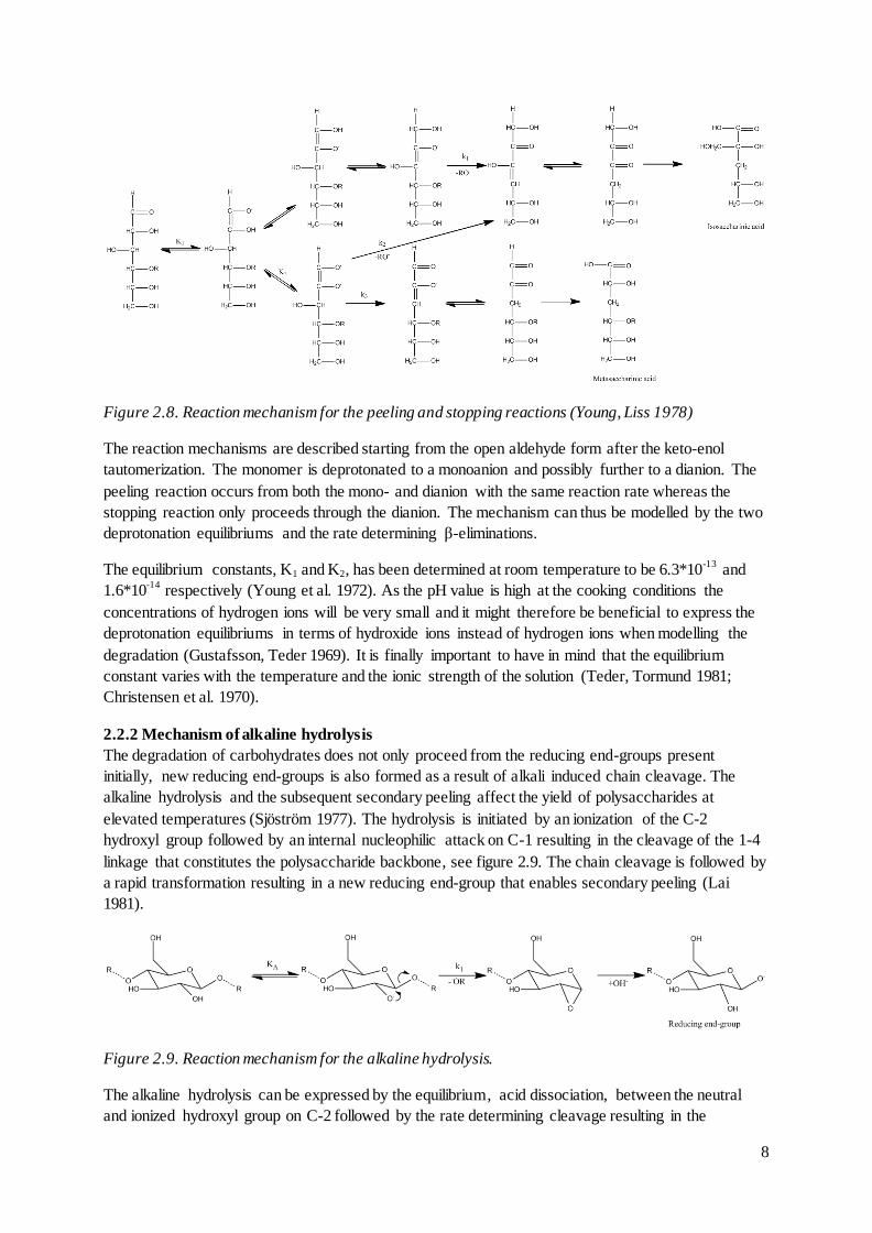
Figure 2.8. Reaction mechanism for the peeling and stopping reactions (Young, Liss 1978)
The reaction mechanisms are described starting from the open aldehyde form after the keto-enol
tautomerization. The monomer is deprotonated to a monoanion and possibly further to a dianion. The
peeling reaction occurs from both the mono- and dianion with the same reaction rate whereas the
stopping reaction only proceeds through the dianion. The mechanism can thus be modelled by the two
deprotonation equilibriums and the rate determining β-eliminations.
The equilibrium constants, K1 and K2, has been determined at room temperature to be 6.3*10-13
and
1.6*10-14
respectively (Young et al. 1972). As the pH value is high at the cooking conditions the
concentrations of hydrogen ions will be very small and it might therefore be beneficial to express the
deprotonation equilibriums in terms of hydroxide ions instead of hydrogen ions when modelling the
degradation (Gustafsson, Teder 1969). It is finally important to have in mind that the equilibrium
constant varies with the temperature and the ionic strength of the solution (Teder, Tormund 1981;
Christensen et al. 1970).
2.2.2 Mechanism of alkaline hydrolysis
The degradation of carbohydrates does not only proceed from the reducing end-groups present
initially, new reducing end-groups is also formed as a result of alkali induced chain cleavage. The
alkaline hydrolysis and the subsequent secondary peeling affect the yield of polysaccharides at
elevated temperatures (Sjöström 1977). The hydrolysis is initiated by an ionization of the C-2
hydroxyl group followed by an internal nucleophilic attack on C-1 resulting in the cleavage of the 1-4
linkage that constitutes the polysaccharide backbone, see figure 2.9. The chain cleavage is followed by
a rapid transformation resulting in a new reducing end-group that enables secondary peeling (Lai
1981).
Figure 2.9. Reaction mechanism for the alkaline hydrolysis.
The alkaline hydrolysis can be expressed by the equilibrium, acid dissociation, between the neutral
and ionized hydroxyl group on C-2 followed by the rate determining cleavage resulting in the

9
degradation products (Lai 1981). The acid dissociation constant has been determined to be 1.84*10-14
at room temperature (Neale 1930). As for the equilibrium constants in the peeling mechanisms, the
acid dissociation constant is not a fixed constant as it is dependent on both temperature and ionic
strength (Pu, Sarkanen 1991; Motomura et al. 1998; Norgren, Lindström 2000).
2.3 Kinetic models for carbohydrate degradation
Kinetic models are a helpful tool for controlling and optimizing the pulping process as well as
providing additional insight into the reaction mechanisms involved. However, the modelling of kraft
cooking kinetics has for a long period of time been focused on the delignification and relatively few
studies have considered the carbohydrate degradation.
The Purdue model developed by Smith and Williams (1974) was the first to study the different
carbohydrates individually and has been subjected to a number of further developments. The Purdue
based models are characterized by the degradation of wood components being described by parallel
phases which are affected to different extents by the cooking conditions, thus accounting for the
changes in degradation behaviour throughout the cook. Another version of phase based models is the
3-stage model as developed by Gustafson et al. (1983) where the degradation is described by
consecutive equations instead of the parallel phases used in the Purdue model. Both phase models aim
to describe the removal of wood material from wood chips and describe the overall effect, including
the mass transfer to and from the wood chips.
Recent work has suggested that the degradation of glucomannan may be described by the usage of the
involved reaction mechanisms instead of phases (Wigell et al. 2007; Paananen et al. 2010), resulting in
increased mechanistic significance of the model parameters (Montané et al. 1998). This is achieved
mainly by modelling the reactions at the reducing end-groups. The reaction mechanism based
approach for xylan removal is less straightforward as alkaline hydrolysis and dissolution of
polysaccharide chains is the dominating mechanisms instead of endwise degradation. The degradation
of xylan may thus rather be described by a continuous distribution of reactivity model. These distinctly
different modelling approaches will be discussed in the following sections.
2.3.1 Phase models
The Purdue- and the 3-stage models are two different families of phase models for describing the kraft
cooking kinetics. The Purdue models describe the degradation by parallel phases representing different
degradation mechanisms whereas the 3-stage models use consecutive reactions, dividing the
degradation into initial, bulk and residual periods.
The Purdue model was initially developed by Smith and Williams (1974) and modelled cellulose,
xylan and glucomannan separately as well as the delignification by dividing lignin into two phases,
high- and low reactive lignin, by using equation (1).
( [
] [ ][ ]) (1)
Where Wi wood component
k rate constants, described by Arrhenius expressions
The Purdue model was later extended by Christensen et al. (1983) in order to better correlate to
experimental data. This was done by adding exponents to the dependence on the hydroxide and
sulphide ion concentrations as well as classifying part of the wood components as unreactive.
( [
] [ ] [ ] )( ) (2)

10
Where Wi wood component
Wi0 unreactive part of wood component
k rate constants, described by Arrhenius expressions
a exponent to the hydroxide ion concentration
b exponent to the sulphide ion concentration
More recent work by Gustavsson and Al-Dajani (2000) has similarly suggested that the degradation of
the different carbohydrates can be described by first order reactions, equations (3) and (4). Their
studies on the latter stages of the cook implied that the degradation of xylan and glucomannan
increased with increasing concentrations of hydroxide ions and hydrogen sulphide, although the effect
of hydrogen sulphide was less prominent for glucomannan. The effect of ionic strength, expressed by
sodium ion concentration, was also considered and found to be insignificant for glucomannan whereas
an increased ionic strength increased the xylan retention. The effect on xylan yield by ionic strength
was suggested to depend on a solubility effect (Gustavsson, Al-Dajani 2000), an explanation that
correlates well with studies of xylan sorption (Ribe et al. 2010).
( ) (3)
( [ ] [
] [ ])
( (
))
(4)
Where a constant describing dissolution at low alkali
k rate constants
EA activation energy
The early Purdue models modelled the individual carbohydrates as degradation in a single phase even
though different reaction mechanisms are assumed to control the degradation during different periods
of the cook (Aurell, Hartler 1965; Sjöström 1977). Gustafson et al. (1983) therefore took another
approach and based the 3-stage model on these differing pulping periods. The 3-stage model describes
the degradation of the combined carbohydrates as dependent on the delignification in each of the
phases by consecutive equations, equations (5)-(10).
Initial phase:
( ) (5)
[ ]
(6)
Bulk phase:
(
(
)[ ]
(
)[ ] [ ] ) (7)
(8)
Residual phase:
(
)[ ] (9)
(10)

11
Where L lignin
C total carbohydrates
S sulphide concentration
The 3-stage model was later improved by Pu et al. (1991) in order to describe the degradation of
hemicelluloses separately from cellulose, as well as independent of delignification, for the initial and
bulk phases.
Initial phase:
( )[ ] ( )
(11)
Bulk phase:
( )[ ]( ) (12)
Where C wood component, either cellulose or hemicellulose
C0 unreactive part of wood component
k rate constants
EA Activation energies
The consecutive phases used in the 3-stage models result in a discontinuous system where the location
of the phase transition is dependent on the cooking conditions (Gustafson et al. 1983). So in order to
improve the accuracy of the Purdue models and avoid the problems that follow the discontinuous 3-
stage model, Andersson et al. (2003) combined their strengths by describing the degradation of all
wood components separately with 3 parallel equations.
([
] [ ] ) (13)
Where W wood component
k1 rate constant, described by Arrhenius expression
k2 constant describing dissolution at low alkali
a exponent to the hydroxide ion concentration
b exponent to the sulphide ion concentration
However, the Andersson model did not vary the model parameters between the different carbohydrates
as it accounted for the differences by variation of the relative magnitude of the different phases. The
phase composition varied with the cooking conditions and thus accounted for a large part of the
modelling (Andersson 2003).
Johansson and Germgård (2007) continued the development of the phase model by accounting for the
different behaviour of individual carbohydrates to varying alkali concentrations as well as by adding a
dependence on the sodium concentration in the cooking liquor. The initial phase composition was also
made independent of the cooking conditions for cellulose and glucomannan and the degradation was
thus described only by the degradation equations. Glucomannan was described by three parallel phases
whereas two phases was sufficient to describe the xylan and cellulose degradations (Johansson,
Germgård 2008). The extent of initial phase xylan was however modelled as dependent on the
hydroxide ion concentration and described by a linear relationship, see equation (15) and (16).

12
([
] [ ] [ ] ) (14)
Where W wood component
k rate constant, described by Arrhenius expression
a exponent to the hydroxide ion concentration
b exponent to the sulphide ion concentration
c exponent to the ionic strength
(15)
[ ] (16)
Where Xi amount of xylan in initial phase
Xf amount of xylan in final phase
The Johansson model was based on experimental data exclusively having cooking times exceeding
100 min and the model does therefore not describe the initial dissolution or primary peeling in detail.
The model is instead focused on the alkaline hydrolysis that dominates the later stages of the cook.
Model parameters for the Johansson model are presented in table 2.3.
Table 2.3. Model parameters for the Johansson model (Johansson, Germgård 2008).
Phase (% ow) A EA [kJ/mol] Hydroxide ion
exponent, a
Sodium ion
exponent, c
Cellulose Initial phase 4.2 1.635E+17 153 1.49 0.58
Final phase 39.8 5.227E+14 151 0.83 0.38
Xylan
Initial phase Xi = 7.61 – Xf 5.840E+17 158 0 -1.35 Final phase Xf = -4.082[OH
-]+6.026 3.444E+16 160 0.62 -0.41
Glucomannan Initial phase 15.5 2.626E+07 70 0 -0.74
Intermediate phase
2.6 3.554E+10 121 0.46 -0.27
Johansson (2008) found that the hemicellulose yield increased with increasing ionic strengths, an
effect that was suggested to be a result of lignin-carbohydrate complexes as lignin dissolution is
retarded by high ionic strengths. However, the carbohydrate degradation was found to not be
significantly affected by the hydrogen sulphide concentration by both Andersson et al. (2003) and
Johansson and Germgård (2007; 2008). These results are contradictory as hydrogen sulphide
influences delignification to a large extent. The increased hemicellulose yield observed at increasing
ionic strengths is most likely rather an effect of decreased solubility of polysaccharide chains and thus
most prominent for xylan (Mitikka-Eklund 1996; Ribe et al. 2010). The ionic strength effect obtained
by Johansson is also most likely overestimated as the experiments used addition of sodium chloride to
adjust the ionic strength. The usage of sodium chloride has later been shown to retard delignification
to a larger extent than other sodium salts more common in industrial black liquor (Bogren et al. 2009a,
Dang et al. 2010).
All the phase based models have been derived from experiments using wood chips of varying
dimensions as raw material. The models are thus not only describing the degradation kinetics, all

13
factors affecting the kinetic behaviour are accounted for jointly. The mass transport of cooking
chemicals to the reaction site in the fibre as well as the diffusion of the degradation products out into
the cooking liquor are effects that may impact the degradation rate significantly when using wood
chips and thus interfere with the reaction kinetics.
2.3.2 Reaction mechanism based models
The phase models aim to describe the carbohydrate degradation either by a single equation or by
combining the effect of a number of different phases. These phases correspond well to the different
reaction mechanisms involved in glucomannan degradation as the initial phase describes the primary
peeling as well as initial dissolution whereas the other two phases represents the slower reacting
alkaline hydrolysis with subsequent secondary peeling. The reaction mechanism based models
describes the reactions more directly by tracking the active sites involved. The effects of cooking
chemicals may be accounted for by the use of either power law equations or the equilibrium constants
associated with intermediates in the reaction mechanism. It is important to note that the reaction
mechanism based model are derived from experiments using wood meal, the effect of mass transport
has thus been minimized in order to isolate the effect of reaction kinetics.
Wigell et al. (2007b) developed a model describing the degradation of glucomannan during soda
cooking using power law equations. The glucomannan yield was calculated by equation (17)-(20)
from the amount of initially insoluble material as well as the degradation through primary peeling and
alkaline hydrolysis.
(17)
( )[
] (18)
( )[
] (19)
( )[
] (20)
Where G glucomannan yield
GIS fraction of glucomannan insoluble in cooking liquor at 25°C
GP fraction removed through primary peeling
GH fraction removed through alkaline hydrolysis and secondary peeling
R frequency of reducing end-groups
k rate constants, described by Arrhenius expressions
l, m, n exponents of the hydroxide ion concentration
After treatment at 25°C and 1.25 mol OH-/kg liquor for 180 min, it was found that 85 % of the
glucomannan remained insoluble (Wigell et al. 2007a). The removal of the 15 % of initially soluble
glucomannan was thus not included in the model. The frequency of reducing end-groups was set to 1
initially and decreased with the stopping reaction whereas the alkaline hydrolysis did not yield
additional reducing end-groups. The effect of secondary peeling is instead accounted for by the
equation for the alkaline hydrolysis (Wigell et al. 2007b).
By studying the parameters for the Wigell model, table 2.4, it can be seen that the stopping reaction is
favoured by an increasing hydroxide ion concentration. Increasing the alkali content will thus result in
a decreased amount of glucomannan degraded through primary peeling whereas simultaneously
increasing the degradation through alkaline hydrolysis and secondary peeling. The relative

14
contribution of the peeling and hydrolysis reactions in the model was validated by cooking series with
wood material pretreated with sodium borohydride. The sodium borohydride prevents primary peeling
as it inactivates the end-groups by acting as a reducing agent, and the subsequent degradation as a
result of the alkaline hydrolysis and secondary peeling was accurately predicted by the model (Wigell
et al. 2007b).
Table 2.4. Model parameters for the Wigell model (Wigell et al. 2007b).
Parameter Value
AP 3.476E+13 AS 4.990E+13
AH 1.495E+08 EA,P 111 kJ/mol
EA,S 110 kJ/mol EA,H 89 kJ/mol
l 0.36 m 0.45
n 0.82
Power law models as the one suggested by Wigell et al. is very flexible in that sense that it is
straightforward to investigate additional effects. The possible influence of ionic strength or the
concentration of hydrogen sulphide is readily added to the model at the expense of an increased
number of model parameters. This straightforward approach is something that models using the
equilibrium constants lack. However, those models instead have the potential to describe the
degradation by using physically relevant parameters only. Paananen et al. (2010) attempted to model
the carbohydrate degradation by taking the equilibrium based approach and modelled the endwise
degradation as suggested by Young et al. (1972).
Figure 2.9. Scheme of the peeling reaction (Young et al. 1972).
The degradation rate for carbohydrates through primary peeling and the corresponding rate of the
stopping reaction can be described by equations (21)-(23).
[ ]
([
] [ ]) (21)
[ ]
[
] (22)
[ ] [ ] [ ] [
] (23)
Where [GE] fraction of material degraded through peeling
[GR]t total fraction of reducing end-groups
[GR-] fraction of mono-ionized end-groups
[GR2-
] fraction of di-ionized end-groups
[GR] fraction of reducing end-groups
k rate constants, described by Arrhenius equations

15
The initial fraction of reducing end-groups was taken as the average of previously published values
(Procter, Apelt 1969; Young, Liss 1978; Jacobs, Dahlman 2001) and set to 0.0075, which corresponds
to a degree of polymerization of 133. The concentrations of the mono- and dianions are in turn
expressed by the equilibriums associated with the ionized end-groups as presented in equations (24)
and (25).
[ ][ ]
[ ] (24)
[ ][ ]
[ ]
(25)
This results in the peeling and stopping reactions being described by equations (26) and (27).
[ ]
([ ] )
[ ] [ ] [ ] (26)
[ ]
[ ] [ ] [ ] (27)
The alkaline hydrolysis contribution was expressed by Paananen et al. (2010) in a similar manner as
presented in figure 2.10 and the corresponding equations (28)-(30).
Figure 2.10. Scheme of the hydrolysis reaction (Paananen et al. 2010).
[ ]
[
] (28)
[ ][ ]
[ ]
[ ][ ]
[ ] [ ] [ ] (29)
[ ]
([ ] [ ])
[ ] (30)
Where [P] fraction of material degraded through alkaline hydrolysis
[GH] fraction of glycoside molecules
[G-] fraction of glycoside anions
k rate constant, described by Arrhenius equation
The set of differential equations (26), (27) and (30) is then solved with the mass balance presented in
equation (31). Similarly to the Wigell model, the initially soluble wood material is omitted from the
degradation model.
[ ] [ ] [ ] [ ] (31)
The model was fitted to experimental data for glucomannan degradation at cooking temperatures
below 130°C, obtaining the model parameters presented in table 2.5. It is important to note that the
model does not account for the temperature dependence of the equilibrium constants and that the
hydrogen ion concentration is calculated from the hydroxide ion concentration using the ionic product
of water at 25°C.

16
Table 2.5. Model parameters for the Paananen model (Paananen et al. 2010).
Parameter Value K1 1.30E-13
K2 7.91E-15 KA 2.22E-15
AP 6.37E15
AS 3.32E14 AH 1.71E12
EA,P 112.5 kJ/mol EA,S 110.6 kJ/mol
EA,H 98.1 kJ/mol GIS 0.96
2.3.3 Continuous distribution of reactivity model
The reaction mechanism based models describes the glucomannan removal as degradation to
monomers through endwise degradation, either through primary peeling or as secondary peeling
following alkaline hydrolysis. This approach is not satisfactory for describing xylan removal as the
effect of endwise degradation is small due to the stabilizing effect of arabinose and glucuronic acid
substituents on the polysaccharide backbone (Whistler, BeMiller 1958; Simonson, 1963; Aurell,
Hartler 1965). The xylan removal is instead dependent on dissolution of longer polysaccharide
fragments. The presence of covalent bonds between lignin and xylan (Lawoko et al. 2005) also have a
retaining effect, and the degradation to soluble fragments are thus obtained through alkaline hydrolysis
of the polysaccharide backbone as well as degradation of lignin and the breakage of lignin-xylan
linkages. The xylan degradation must thus be considered as part of a more complex system and
affected by a variety of reactions and effects with contributions that vary during different stages of the
cook.
The continuous distribution of reactivity model describes the degradation by assuming that the
activation energy of the reactions contributing to the degradation is continuously distributed. The
degradation is assumed to occur through first order kinetics with a time-dependent rate constant
accounting for the varying behaviour throughout the cook. While the phase models are considering the
studied wood component to consist of a finite number of fractions with different reactivities, the
continuous distribution of reactivity model rather assumes the material to consist of a very large
number of similar chemical species (Montané et al. 1998). Variations of the continuous distribution of
reactivity approach has previously been used on biomass for modelling of delignification (Montané et
al. 1994; Bogren et al 2008b) as well as xylan degradation during dilute acid hydrolysis of birch
(Montané et al. 1998). These models used an expression for the time-dependent rate constant proposed
for species trapped in condensed media, see equation (32) (Plonka 1986).
( ) (32)
Where β time independent rate constant
γ dispersion factor
The parameter γ describes the dispersion of the system with a value of 1 corresponding to classical
kinetics and thus no dispersing effect. Using this rate constant, the xylan degradation may be described
by equation (33).
(33)

17
As the system may be described as a multitude of simultaneous degradation reactions, it is preferably
describe by using the Kohlrausch relaxation function. The Kohlrausch relaxation function can be seen
as the superposition of exponential decays and may be reached by defining the effective lifetime
according to equation (34) (Plonka 1986), resulting in the mean lifetime as expressed by equation (35)
(Bogren et al. 2008b).
(
)
(34)
(
) (
) (35)
Where effective lifetime of wood component in cooking liquor
mean lifetime of wood component in cooking liquor
Γ gamma function, defined according to equation (36)
( ) ∫
(36)
The mean lifetime of the modelled wood component may also be expressed as the inverse of a time-
independent rate constant according to equation (37).
( ([ ] [ ] [ ])
)
(37)
Where S pre-exponential factor, dependent on liquor composition
mean activation energy of degradation reactions
The pre-exponential factor in equation (37) is dependent on the cooking liquor composition and
accounting for the effects of cooking chemicals on the degradation rate. A standard power law
expression is however not sufficient to describe the effect of cooking chemicals as the dependence is
changing throughout the cook. Bogren et al. (2008b) modelled delignification with the continuous
distribution of reactivity model by using a modified power law expression, making the exponents
linearly dependent on the degree of delignification, see equation (38).
([ ] [ ] [ ]) ([ ] [ ] [ ] ) (38)
Combining equations (33)-(37) and using the modified power law expression in equation (38) yields
the continuous distribution of reactivity model according to equation (39).
( ([
] [ ] [ ] )
)
(
)
(39)
When modelling the delignification Montané et al. (1994) found the relaxation parameter, γ, to
increase with increasing cooking temperatures. Bogren et al. (2008b) suggested that describing the
parameter as linearly dependent of the temperature, equation (40), increased the model performance
significantly. Including a linear temperature dependence of the system dispersion in the continuous
distribution of reactivity model results in 10 parameters required to describe the xylan removal.
(40)

18
3. Method
3.1 Experimental methods
This thesis is based on extensive experimental data for kraft cooking of wood meal at constant liquor
composition in autoclaves. A detailed description of the experimental procedure is given by Bogren
(2008), Bogren et al. (2007) and Bogren et al. (2009b) whereas a brief summary is presented in the
following section. Additional experimental data concerning alkaline cooking was obtained with a
similar experimental method from the work of Wigell et al. (2007a), whereas the effect of varying
ionic strength were investigated by Dang et al. (2010) using a flow through reactor.
The raw material used for all experiments was sapwood from Scots pine (Pinus sylvestris) originating
from the southwest of Sweden. The wood meal was produced in a Wiley mill with screens allowing
particles with a diameter below 1 mm to pass, thus minimizing the effect of mass transport throughout
the cooking process. In order to minimize unwanted degradation during storage, the wood meal was
stored frozen without pre-drying.
In the cooking experiments the liquor to wood ratio was high (200:1) in order to ensure constants
chemical conditions throughout the cook. The studied cooking temperatures ranged from 108-168°C
while the concentrations of hydroxide ions and hydrogen sulphide were varied between 0.1-0.78
mol/kg solvent and 0.1-0.52 mol/kg solvent respectively. The cooking liquors were prepared from
analysis graded Na2S and NaHS and reagent graded NaOH dissolved in deionized water. The ionic
strength of the liquor can thus be expressed by the sodium ion concentration. Apart from the standard
kraft cooking experiments additional series using wood material pretreated with sodium borohydride
was included. The sodium borohydride addition reduces the end-groups and thus prevents primary
peeling, allowing for the degradation through alkaline hydrolysis to be studied separately.
Validation series using a liquor to wood ratio of 7:1 were performed in order to be more comparable to
an industrial cook. The concentrations of the active cooking chemicals was not constant during these
trails but was measured by titration and the variation can thus be included in the modelling. During the
validation trails both synthetic liquors prepared from salts and industrial liquors were used.
All cooking experiments were performed in autoclaves rotating in a pre-heated polyethylene glycol
bath in order to reach the desired cooking temperature. As pretreatment the autoclaves were evacuated
for 5 minutes and the subjected to a pressure of 0.5 MPa of nitrogen for 5 minutes in order to achieve
an oxygen-free environment and good impregnation during the cook. The over-pressure was released
before the cooking was initiated. The temperature was measured during the heating up period of the
autoclaves and this period was included in the cooking time, the temperature rise must thus be
described in the modelling. The cook was terminated at the desired cooking time by cooling the
autoclave with running tap water for 15 minutes. The content was then washed with 0.5 l of cooking
liquor filtrate and 1 l of deionized water. The carbohydrate content was determined from the filtrate
using IC with pulsed amperometric detection (CarboPacTM
PA1 column, Dionex, Sunnyvale, CA,
USA). The experimental error of the measurement of carbohydrates in the wood after cooking was
determined to be ± 3 % based on six analyses of untreated wood meal.
3.2 Mathematical modelling methods
During the early part of the cooking experiments, the temperature rises in the autoclaves as the
polyethylene glycol bath is preheated to the cooking temperature whereas the autoclaves are room
tempered. This temperature rise is included in the modelling as the temperature is described by
equation (41).

19
( ) ( ) (41)
Where Tmax cooking temperature, expressed in Kelvin
Tstart room temperature, 293.15 K
t cooking time, expressed in minutes
All modelling was performed using the Matworks Inc. Matlab 7.11 software with the optimization and
statistical toolboxes. The systems of differential equations constituting the models were solved using
ode113 which is suitable for computationally intensive problems. The model parameters were fitted to
the experimental data by using the commands nlinfit and fmincon. To avoid optimizing the model
around a local minimum the parameter optimization was performed by using the GlobalSearch
algorithm which uses multiple initial guesses for the parameters. The residual used throughout the
parameter optimization was the squared difference between the model value and the experimentally
obtained value.
( ) (42)
The model fit was evaluated using the coefficient of determination, R2. The coefficient of
determination is a statistical measure of how large fraction of the experimental variance that is
described by the fitted model and is calculated by equation (43). A coefficient of determination of 1
thus means the model describes all variation in the experimental data.
∑( )
∑( ) (43)
Where experimental value
mean value of the experimental data
model value
The standard error of estimation, equation (44), was also used as a measure of the model performance.
This corresponds to the deviations in [yield %]; the standard deviation expressed in [% on wood] is
obtained by multiplication with the initial fraction of the wood component.
√∑( )
(44)
Where Sy,x standard error of estimation
n number of experiments
The error of estimation expressed as % of the experimentally measured amount of glucomannan can
be calculated by equation (45). This value is suitable to comparison with the experimental error of
3 %.
∑| |
(45)

20
4. Results and discussion This chapter contains the results of the thesis. The experimental data used for modelling of
glucomannan and xylan removal is presented initially along with a discussion of the mechanisms
behind the observed degradation effects. The modelling of glucomannan degradation was performed
using reaction mechanism based approaches whereas the removal of xylan was described by phase
models as well as a continuous distribution of reactivity model. The degradation models are then
validated with experimental data from other authors at differing experimental conditions.
4.1 Carbohydrate degradation and dissolution
4.1.1 Effect of temperature
The degradation of hemicelluloses is strongly temperature dependent as both reaction rate and final
yield is affected by the cooking temperature. The yield difference arise from the decreased alkaline
hydrolysis at lower cooking temperatures whereas the extent of the primary peeling is largely
unaffected by the temperature, see figure 4.1 and 4.2. The yield differences at varying cooking
temperatures are thus larger for xylan than glucomannan due to the stabilizing effect of arabinose side-
groups towards endwise degradation (Whistler, BeMiller 1958; Sjöström 1977). This stabilizing effect
is decreased at increasing temperatures as a result of substituent removal through alkaline hydrolysis
yielding additional secondary peeling (Simonson 1963; Simonson, 1965; Hansson, Hartler 1968).
Another effect that was observed from the experimental results was that the rate of glucomannan
degradation was significantly decreased as the yield approached 20 %. This effect of a residual
glucomannan that is rather stable towards degradation has been suggested to depend on a fraction of
glucomannan with a more ordered structure, thus shielding the glucosidic linkages against alkaline
hydrolysis (Aurell, Hartler 1965).
Figure 4.1. Temperature dependence of the glucomannan degradation at liquor composition of OH
-
=0.26 mol/kg solvent, HS-=0.26 mol/kg solvent, Na
+=0.52 mol/kg solvent.

21
Figure 4.2. Temperature dependence of the xylan degradation at liquor composition of OH
-=0.26
mol/kg solvent, HS-=0.26 mol/kg solvent, Na
+=0.52 mol/kg solvent.
4.1.2 Effect of hydroxide ion concentration
The degradation of glucomannan and xylan are affected differently by the hydroxide ion concentration
as a result of the primary degradation mechanisms involved. An increased hydroxide ion concentration
limits the extent of primary peeling as the selectivity for the chemical stopping reaction is benefitted
from the increasing alkali, see figure 4.3. The reaction rate of both the peeling and stopping reactions
are increased by a higher hydroxide ion concentration, but the selectivity for the stopping reaction is
increased as the stabilizing formation of metasaccharinic acid requires a dianion intermediate whereas
the peeling reaction can occur through either mono- or dianion intermediates. An increased hydroxide
ion concentration increases the fraction of dianionic end-groups and thus increases the reaction rate of
the stopping reaction to a higher degree than the reaction rate of the peeling reaction (Lai, Sarkanen
1969; Young et al. 1972).
Increasing the hydroxide ion concentration also increases the degradation through alkaline hydrolysis.
The alkaline hydrolysis is strongly dependent on the hydroxide ion concentration as the reaction is
initiated by the deprotonation of hydroxyl groups on the polysaccharide backbone (Lai 1981). The
trend that can be observed in figure 4.3 is thus that an increased hydroxide ion concentration lowers
the glucomannan degradation through primary peeling in the early part of the cook. The glucomannan
degradation is instead increased in the latter stages of the cook where alkaline hydrolysis and
subsequent secondary peeling is the dominating degradation mechanisms. The limiting effect of a high
hydroxide ion concentration on the degradation through primary peeling can also be seen at lower
cooking temperatures, figure 4.4, where the degradation through alkaline hydrolysis is less prominent.
In this case is the degradation rate decreased initially by a lower hydroxide ion concentration, but the
stopping reaction is decreased even further resulting in a lower glucomannan yield. It should however
be noted that the overall effect of varying hydroxide ion concentrations on the glucomannan
degradation is relatively minor.

22
Figure 4.3. Effect of the hydroxide ion concentration on glucomannan degradation at 168°C, HS
-
=0.26 mol/kg solvent.
Figure 4.4. Effect of the hydroxide ion concentration on glucomannan degradation at 139°C, HS
-
=0.26 mol/kg solvent.
The effect of the hydroxide ion concentration on xylan degradation is more straightforward than for
glucomannan degradation as a higher alkali increases the removal during all stages of the cook, see
figure 4.5. This is the case as xylan degradation is dominated by alkaline hydrolysis resulting in both
chain cleavage as well as removal of the arabinose side-groups, thus increasing the extent of secondary
peeling obtained from each formed reducing end-group (Aurell, Hartler 1965; Hansson, Hartler 1968).
The xylan removal is also benefitted by an increased solubility of polysaccharide fragments at
increased hydroxide ion concentrations (Yllner, Enström 1956; Hansson, Hartler 1969; Ribe et al.
2010).

23
Figure 4.5. Effect of the hydroxide ion concentration on xylan degradation at 168°C, HS
-=0.26 mol/kg
solvent.
4.1.3 Effect of hydrogen sulphide concentration
Previous studies have found that an increase in hydrogen sulphide concentration increases the removal
of carbohydrates slightly (Lémon, Teder 1973; Gustavsson, Al-Dajani 2000; Johansson 2008). This
effect may be explained by increased accessibility and less retention due to lignin-carbohydrate
linkages as a result of improved delignification. The hydrogen sulphide concentration has been found
to have a more pronounced effect on the removal of xylan than glucomannan (Gustavsson, Al-Dajani
2000), figure 4.6 and 4.7, which correlates well with the lignin-carbohydrate complexes explanation as
xylan has been found to be more closely associated with lignin (Lawoko et al. 2005).
Figure 4.6. Effect of the hydrogen sulphide concentration on glucomannan degradation at cooking
temperatures of 108°C(Δ) and 168°C(○) with OH-=0.26 mol/kg solvent.

24
Figure 4.7. Effect of the hydrogen sulphide concentration on xylan removal at OH
-=0.26 mol/kg
solvent and temperatures 108°C(□), 139°C(Δ) and 168°C(○).
The experimental data suggests a slight increase in the extent of glucomannan removal at higher
concentrations of hydrogen sulphide, although the trend is less conclusive than the effects of
hydroxide ion concentration and temperature. The retaining effect of lignin-carbohydrate complexes
on the glucomannan removal may be limited compared to the effect on xylan because of the rapid
degradation of glucomannan to monomers. There are however significant covalent bonding between
glucomannan and lignin (Lawoko et al. 2005), as has been shown by the decreased rate of
delignification obtained when the glucomannan degradation through primary peeling is impaired
(Wilson, Procter 1970; Bogren 2008).
An increased glucomannan removal at higher hydrogen sulphide concentrations would be a result of
improved accessibility and less retention from lignin-glucomannan complexes. The glucomannan
yield at a given degree of delignification should thus be either unchanged or slightly increased as the
selectivity for lignin degradation is improved. This would be the case as the addition of hydrogen
sulphide improves the rate of delignification, thus yielding the degree of delignification more rapidly
and lowering the glucomannan degradation achieved. As can be seen in figure 4.8, this effect is not
conclusive for the used experimental data. It is thus possible that the relatively minor differences in
glucomannan yield between varying hydrogen sulphide concentrations largely arise from experimental
error.

25
Figure 4.8. Effect of the hydrogen sulphide concentration on glucomannan degradation at OH
-=0.26
mol/kg solvent and cooking temperatures 108°C(Δ) and 168°C(○).
The removal of xylan has a clear dependence of the hydrogen sulphide concentration, even though
hydrogen sulphide is not considered to contribute directly to xylan degradation. As both glucomannan
and xylan form lignin-carbohydrate complexes (Lawoko et al. 2005) it is unlikely that the closer
affinity of xylan to lignin, resulting in a more pronounced increase in accessibility, is enough to
explain the difference. A plausible explanation is rather that the glucomannan removal is less affected
by the degree of delignification as the removal largely is achieved by endwise degradation forming
monomers in the early stages of the cook. The removal of xylan on the other hand is constituted of
dissolution of polysaccharide chains and the decreased solubility obtained by the presence of lignin-
carbohydrate complexes thus impact the removal to a larger extent. This is shown by the fact that
delignification and xylan removal is closely associated, see figure 4.9.
Figure 4.9. Effect of the hydrogen sulphide concentration on xylan removal at OH
-=0.26 mol/kg
solvent and temperatures 108°C(□), 139°C(Δ) and 168°C(○).

26
4.1.4 Effect of ionic strength
The ionic strength of the cooking liquor, measured as sodium ion concentration, has been found to
influence the cooking kinetics by retarding the delignification (Lémon, Teder 1973; Teder, Olm 1981;
Lindgren, Lindström 1996; Bogren et al. 2009a). This retarding effect has been suggested to depend
on a decreased solubility of lignin fragments and the effect has been shown to vary depending on the
salt composition of the liquor (Norgren et al. 2002; Bogren et al 2009a). The effect is especially
pronounced for experiments using addition of sodium chloride, as chloride ions have been shown to
affect the delignification to a larger extent than the anions present in industrial liquors (Bogren et al.
2009a; Dang et al. 2010). Xylan removal, which is dependent on dissolution of larger polysaccharide
fragments, has similarly been shown to decrease with an increasing sodium ion concentration, figure
4.10 (Dang et al. 2010). This effect also arises from a decreased solubility as studies have shown that
sorption of xylan onto cellulose fibres is increased at increasing ionic strengths (Ribe et al. 2010).
Figure 4.10. Effect of the ionic strength at 168°C with OH
-=0.26 mol/kg solvent and HS
-=0.26 mol/kg
solvent. The ionic strength was achieved through addition on sodium carbonate.
The removal of glucomannan has been shown to remain largely unaffected at various ionic strengths,
see figure 4.11 (Dang et al. 2010; Dang et al. 2011). This is somewhat expected as the removal is less
dependent on solubility due to the extensive endwise degradation. It does however imply that Donnan
effects lack significant impact on the glucomannan degradation. Donnan membrane equilibrium theory
states that the concentration of hydroxide ions is lower in the fibre wall than in the bulk liquor due to
the fibres negatively charged surface. This concentration difference decreases at increasing ionic
strengths as a result of screening of the negative charges on the surface (Pu, Sarkanen 1991;
Motomura et al. 1998). The occurrence of significant Donnan effects at the prevailing cooking
conditions has been found by studying the formation and degradation of hexenuronic acid (Bogren et
al. 2008a). The endwise degradation reactions are however not as strongly affected by the hydroxide
ion concentration as the hexenuronic acid reactions, thus limiting the Donnan effects on the overall
glucomannan degradation.

27
Figure 4.11. Effect of the ionic strength at 168°C with OH
-=0.26 mol/kg solvent and HS
-=0.26 mol/kg
solvent. The ionic strength was achieved through addition on sodium carbonate.
4.2 Modelling of glucomannan degradation
The following sections are focused on describing the glucomannan degradation during kraft pulping
by using models based on the main reaction mechanisms involved. Whereas phase based models are
useful for describing existing experimental data, reaction mechanism based models allow for
additional insight through the usage of parameters with distinct physical meaning. The modelling
performed in the following sections is based on two levels of reaction mechanism models. The model
proposed by Wigell et al. (2007) uses a straightforward mathematical approach of describing the
effects of cooking chemicals through power law expressions, whereas the model published by
Paananen et al. (2010) uses the equilibrium constants of rate limiting intermediates.
4.2.1 Wigell model
The power law based model for glucomannan degradation as proposed by Wigell et al. (2007b) was
solved using equations (45)-(49).
(45)
( )[
] (46)
( )[
] (47)
( )[
] (48)
(49)
Where G glucomannan yield
GIS fraction of glucomannan insoluble at 25°C, 0.85 (Wigell et al. 2007a)
GP fraction removed through primary peeling
GH fraction removed through alkaline hydrolysis and secondary peeling
t cooking time, expressed in minutes
R(t) frequency of reducing end-groups
28
k rate constants, described by Arrhenius expressions
l, m, n exponents of the hydroxide ion concentration
A pre-exponential factor
EA activation energy
R ideal gas constant
The model was fitted to the experimental data while excluding experimental values exceeding the
fraction of insoluble glucomannan at 25°C. This was done in order to limit the deviation originating
from the initial dissolution not included in the model and rather model the actual degradation
reactions. The initial conditions used in the model is GP = 0, R = 1 and GH = 0.
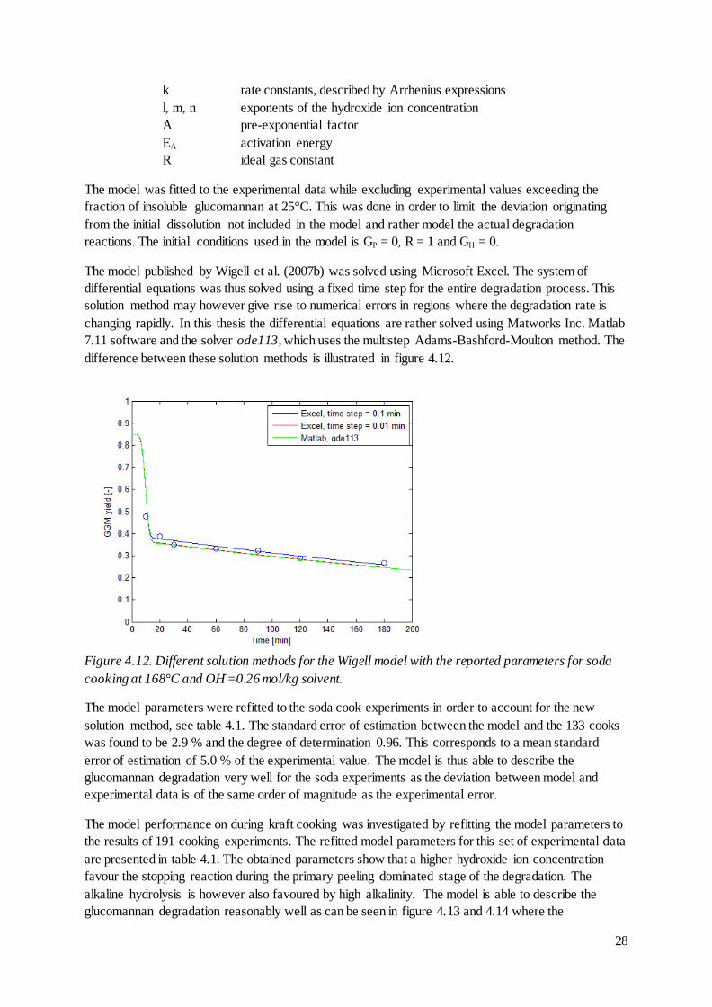
The model published by Wigell et al. (2007b) was solved using Microsoft Excel. The system of
differential equations was thus solved using a fixed time step for the entire degradation process. This
solution method may however give rise to numerical errors in regions where the degradation rate is
changing rapidly. In this thesis the differential equations are rather solved using Matworks Inc. Matlab
7.11 software and the solver ode113, which uses the multistep Adams-Bashford-Moulton method. The
difference between these solution methods is illustrated in figure 4.12.
Figure 4.12. Different solution methods for the Wigell model with the reported parameters for soda
cooking at 168°C and OH-=0.26 mol/kg solvent.
The model parameters were refitted to the soda cook experiments in order to account for the new
solution method, see table 4.1. The standard error of estimation between the model and the 133 cooks
was found to be 2.9 % and the degree of determination 0.96. This corresponds to a mean standard
error of estimation of 5.0 % of the experimental value. The model is thus able to describe the
glucomannan degradation very well for the soda experiments as the deviation between model and
experimental data is of the same order of magnitude as the experimental error.
The model performance on during kraft cooking was investigated by refitting the model parameters to
the results of 191 cooking experiments. The refitted model parameters for this set of experimental data
are presented in table 4.1. The obtained parameters show that a higher hydroxide ion concentration
favour the stopping reaction during the primary peeling dominated stage of the degradation. The
alkaline hydrolysis is however also favoured by high alkalinity. The model is able to describe the
glucomannan degradation reasonably well as can be seen in figure 4.13 and 4.14 where the

29
dependence of temperature and hydroxide ion concentration are shown.
Figure 4.13. The temperature dependence of the Wigell model with a liquor composition of OH
-=0.26
mol/kg solvent, HS-=0.26 mol/kg solvent, Na
+=0.52 mol/kg solvent.
Figure 4.14. The hydroxide ion dependence of the Wigell model at 168°C and with a liquor
composition of HS-=0.26 mol/kg solvent.
The standard error of estimation for the Wigell model on the kraft cooking experiments was found to
be 4.3 % and the coefficient of determination was calculated to 0.94. The Wigell model only account
for temperature and hydroxide ion concentration and thus lack the ability to describe possible effect of
varying hydrogen sulphide concentration. Part of the deviation between model and experimental data
arise from series with differing hydrogen sulphide concentration, as is indicated by figure 4.15. In
order to evaluate the significance of hydrogen sulphide to the overall model fit, the Wigell model was
modified to include this aspect by increasing the number of model parameters, see equation (50)-(52).

30
Figure 4.15. Predictions of the Wigell model plotted against the experimental data.
( )[
] [ ] (50)
( )[
] [ ] (51)
( )[
] [ ] (52)
The model parameters were refitted, see table 4.1, and only minor effects on the overall model
performance were observed as the standard error of estimation were calculated to be 4.1 %. The
parameter for hydrogen sulphide dependence of the alkaline hydrolysis was found to be insignificant
and was excluded from the model whereas a higher concentration benefitted the degradation through
primary peeling.
Figure 4.16. Predictions of the Wigell model with hydrogen sulphide dependence, plotted against the
experimental data.

31
Figure 4.17. The hydrogen sulphide dependence of the modified Wigell model at 108°C (□) and 168°C
(○) with a hydroxide ion concentration of 0.26 mol/kg solvent.
Table 4.1. Model parameters for the Wigell model and the Wigell model with hydrogen sulphide
dependence when fitted to soda cooking experiments and kraft cooking experiments.
Parameter Wigell model, Soda
cooking experiments
Wigell model, Kraft
cooking experiments
Wigell HS- model, Kraft
cooking experiments
AP 4.057E+13 4.975E+13 5.086E+13 AS 6.290E+13 4.978E+13 4.951E+13 AH 6.505E+07 2.271E+10 2.142E+08 EA,P 111.4 kJ/mol 111.0 kJ/mol 111.0 kJ/mol EA,S 110.1 kJ/mol 108.9 kJ/mol 109.0 kJ/mol EA,H 86.2 kJ/mol 107.7 kJ/mol 106.7 kJ/mol l 0.397 0.354 0.345
m 0.497 0.396 0.388 n 0.744 0.485 0.458
p - - 0.030 q - - -0.012
r - - -
4.2.2 Equilibrium based model
Paananen et al. (2010) proposed a model describing the glucomannan degradation by using the
equilibrium constants involved in the reaction mechanisms. The Paananen model was solved using
equations (53)-(56).
[ ] [ ] [ ] [ ] (53)
[ ]
([ ] )
[ ] [ ] [ ] (54)
[ ]
[ ] [ ] [ ] (55)

32
[ ]
([ ] [ ])
[ ] (56)
Where [G]t fraction of glucomannan remaining
[GIS] fraction of glucomannan insoluble at 25°C
[GE] fraction of material degraded through primary peeling
[P] fraction of material degraded through alkaline hydrolysis
[GR]t total fraction of reducing end-groups
k rate constants, described by Arrhenius expressions
K equilibrium constants according to figure 2.9 and figure 2.10
The initial conditions used were GE = 0, P = 0 and GR = 0.0075 while 96 % of the glucomannan was
considered insoluble at room temperature. The model was able to describe the experimental data
published by Paananen et al. (2010) very well as the solution method used in this thesis yielded a
standard error of estimation of 2.7 % and a coefficient of determination of 0.99. When studying the
contribution of the primary peeling and the degradation through alkaline hydrolysis individually it can
however be seen that the alkaline hydrolysis dominates the glucomannan degradation already at low
cooking temperatures.
Figure 4.18. Contribution of primary peeling and alkaline hydrolysis to the degradation of
glucomannan according to the Paananen model at a cooking temperature of 105°C with OH- = 0.93
mol/l and 33 % sulphidity.
The unexpected behaviour of the alkaline hydrolysis originates from the equilibrium expression used
in the derivation of the model, see equation (29). This expression suggests that the amount of
glucomannan not in ionized form is described by equation (57), which cannot be the case when
considering the mass balance in equation (53).
[ ] [ ] [ ] [ ] [ ] [ ] [ ] [
] (57)
The amount of glucomannan removed through alkaline hydrolysis and secondary peeling, [P], already
is accounted for when determining [G]t and the amount of glucomannan susceptible for deprotonation
should thus rather be described by equation (58).
[ ] [ ] [ ] [ ] [ ] [ ] [
] (58)

33
That is, the amount of glucomannan that may be deprotonised is the same as the remaining
glucomannan except for the ionized fraction. Using this expression, the equilibrium takes the form of
equation (59) and the removal of glucomannan through alkaline hydrolysis is described by equation
(60).
[ ][ ]
[ ]
[ ][ ]
[ ] [ ] (59)
[ ]
[ ]
[ ] (60)
In the Paananen model, the hydrogen ion concentration is calculated from the hydroxide ion
concentration by using the ionic product of water at 25°C. As the ionic product of water is strongly
dependent on the temperature (Olofsson, Hepler 1975) it is appropriate to rather express the
equilibriums by using the hydroxide ion concentration directly.
[ ]
[ ][ ] (61)
[ ]
[ ][ ]
(62)
[ ]
[ ][ ]
[ ]
[ ]([ ] [ ]) (63)
Note that the equilibrium constants in these cases represent the ratio of the equilibrium constant using
the hydrogen ion concentration and the ionic product of water. With this representation of the
equilibriums, the degradation of glucomannan may be modelled by an equilibrium based model using
equations (64)-(67).
[ ] [ ] [ ] [ ] (64)
[ ]
[ ]
[ ] [ ] ( [
])[ ] (65)
[ ]
[ ]
[ ] [ ] [
][ ] (66)
[ ]
[ ]
[ ]( [ ] [ ]) (67)
When fitting the model parameters in the equilibrium based model described by equations (64)-(67),
see table 4.2, an equally satisfactory description of the experimental data from the studies of Paananen
et al. (2010) was obtained. The degradation through alkaline hydrolysis is however low as the cooking
temperatures used were below 130°C and the corresponding model parameters were thus not
statistically relevant. The glucomannan removal could therefore be described solely by the endwise
degradation reactions, yielding a standard error of estimation of 3.1 % and a coefficient of
determination of 0.98. The primary peeling is thus accounting for the glucomannan degradation in the
equilibrium based model, as can be seen in figure 4.19. This behaviour corresponds well with
experiments where the primary peeling reaction has been disabled by reduction of the end-groups
through sodium borohydride addition considering the high temperature dependence of the alkaline
hydrolysis (Wigell et al. 2007a), see figure 4.20.

34
Figure 4.19. Contribution of primary peeling and alkaline hydrolysis to the equilibrium based model
at 105°C, OH- = 0.93 mol/l and 33 % sulphidity. Note that the alkaline hydrolysis reaction is
inactivated due to parameter insignificance when using experimental data from the temperature range
80-130°C.
Figure 4.20. Effect of sodium borohydride addition at a liquor composition of OH
-=0.78 mol/kg
solvent and HS-=0.52 mol/kg solvent. Sodium borohydride addition (Δ), reference (○).
Refitting the equilibrium based model to the kraft cooking experiments used in this thesis results in the
model parameters presented in table 4.2. As for the evaluation of the Wigell model the fraction of
insoluble glucomannan was set to 85 % and yields exceeding this value were omitted. The model
performance was similar to the Wigell model in describing the temperature and hydroxide ion
dependence of the degradation, as can be seen in figures 4.21 and 4.22 respectively. The standard error
of estimation for the equilibrium based model was calculated to be 4.3 % with a coefficient of
determination of 0.94. The equilibrium based model is thus able to represent the experimental data
with the same level of accuracy as the power law based model.

35
Table 4.2. Model parameters for the equilibrium based model fitted to the experimental data published
by Paananen et al. (2010) as well as the kraft cooking experiments performed by Bogren (2008).
Parameter Equilibrium based model,
Paananen cooking experiments
Equilibrium based model,
Bogren cooking
experiments
K1 1.008 1.306 K2 10.66 105.6
KA - 3.082 AP 5.82E+14 4.00E+15
AS 3.55E+12 2.94E+13 AH - 1.29E+10
EA,P 103.4 kJ/mol 110.6 kJ/mol EA,S 100.4 kJ/mol 108.5 kJ/mol
EA,H - 104.9 kJ/mol GIS 0.96 0.85
Figure 4.21. The temperature dependence of the equilibrium based model with a liquor composition of
OH-=0.26 mol/kg solvent, HS
-=0.26 mol/kg solvent, Na
+=0.52 mol/kg solvent.

36
Figure 4.22. The hydroxide ion dependence of the equilibrium based model at 168°C and with a liquor
composition of HS-=0.26 mol/kg solvent.
When studying the model parameters in table 4.2, the equilibrium constants are noteworthy. As the
equilibrium constants are considered to not vary in the investigated temperature interval, the
equilibrium constant expressed by hydrogen ions is thus assumed to follow the temperature
dependence of the ionic product of water. This assumption is made for modelling purposes in order to
limit the number of parameters and is not strictly valid. The equilibrium constant for deprotonation has
in fact been shown to increase less rapidly than the ionic product of water at increasing temperatures
(Pu, Sarkanen 1991). The assumption thus results in the equilibrium constants overly favouring the
reactions at higher temperatures, an effect that the model counteracts by lowering the activation
energies. The obtained activation energies can thus be assumed to be slightly lower than the actual
activation energies. The calculated values for the equilibrium constants as expressed in hydrogen ion
form at both ends of the investigated temperature interval are presented in table 4.3 along with
corresponding literature values.
Table 4.3. Literature values and modelling results of the equilibrium constants with equilibriums
expressed as dependent on hydrogen ion concentration.
Compound T [°C] pK1 pK2 pKA Reference
Glucomannan 80 12.6 11.6 - Model value, Paananen data Glucomannan 130 11.9 10.8 - Model value, Paananen data
Glucomannan 108 12.0 10.1 11.7 Model value, Bogren data Glucomannan 168 11.4 9.47 11.0 Model value, Bogren data
Cellulose 25 - - 13.7 Neale 1930
Cellulose 25 - - 14.0 Pu, Sarkanen 1991 Glucose 25 12.1 13.8 - Bamford, Collins 1950
Laminarin 56 12.2 - - Young et al. 1972 Glucose 10 12.7 - - Christensen et al. 1970
Glucose 25 12.3 - - Christensen et al. 1970 Mannose 10 12.5 - - Christensen et al. 1970
Mannose 40 11.8 - - Christensen et al. 1970

37
The monoanion equilibrium constant obtained from the model are in good agreement with the
literature values which mostly were derived from monosaccharides. There are however significant
deviation between the literature values and the model values for the equilibriums concerning both the
stopping and alkaline hydrolysis reactions. In both cases are the values from the model implying that
the ionized forms occur to a higher degree than the literature value suggests and that the reaction rates
thus are less dependent on the hydroxide ion concentration. This behaviour is a result of the model
formulation as additional effects are modelled by the equations in the currently used form. The
contribution of physical stopping of the endwise degradation is not accounted for separately as the
model only include the chemical stopping reaction. As the physical stopping is independent of the
alkali, the overall effect of hydroxide ion concentration is thus decreased compared to the pure
chemical stopping reactions described by the literature values. Plausible explanations to this physical
stopping is formation of metasaccharinic acid induced by branching or linkages to either lignin or
other polysaccharides, as well as the complete degradation of a polysaccharide chain as both these
actions result in the removal of a reducing end-group.
The effect of hydroxide ion concentration on the relative rates of the propagation and termination
reactions can be seen in figure 4.23 for the rate constants obtained through fitting the model to the
kraft cooking experiments of Bogren and Paananen respectively. The relatively minor effect of
hydroxide ion concentration on the yield, see figure 4.3 and 4.4, implies that the apparent equilibrium
constant with the applied model formulation cannot approach the literature value while describing the
degradation sufficiently. An alkali independent physical stopping term would rather be needed to limit
the propagation to termination ratio at low hydroxide ion concentrations.
Figure 4.23. Ratio of peeling and stopping reaction at 100°C according to the equilibrium based
model.
The equation modelling the alkaline hydrolysis is also describing additional functions. It does not only
include the chain cleavage reaction, it also describes the degradation through secondary peeling. This
additional effect has a substantial impact on the model value for the corresponding equilibrium
constant. The model may however readily be modified so that the alkaline hydrolysis gives rise to new
reducing end-groups whereas the secondary peeling is accounted for by the peeling equations. The
degradation is thus described by equations (68)-(70).
[ ] [ ] [ ] (68)

38
[ ]
[ ]
[ ] [ ] ( [
])[ ] (69)
[ ]
[ ]
[ ] [ ] [
][ ] [
]
[ ]( [ ]) (70)
With this configuration a different set of model parameters are obtained, see table 4.4. The equilibrium
constant for the alkaline hydrolysis corresponds better to the literature value as the pKa value was
found to be 13.8 and 13.2 at the ends of the temperature interval. The ability of the model to describe
the glucomannan degradation is however decreased by the increased coupling of model equations,
rendering it less useful for description of the degradation. This difference is significant at high
temperatures and high alkalinity where the alkaline hydrolysis reaction is pronounced, as can be seen
in figure 4.24 where the coupled and uncoupled models are compared. This implies that the reducing
end-groups created from alkaline hydrolysis cannot be treated similarly as the primary reducing end-
groups as this results in an overestimation of the secondary peeling. A larger extent of physical
stopping may be expected on the secondary reducing end-groups due to the lower degree of
polymerisation of these polysaccharide fragments. The overall standard error estimation of the coupled
equilibrium based model was however not largely affected as the majority of the cooking experiments
used less severe conditions, thus having a limited contribution of secondary peeling. The standard
error estimation found to be 4.6 % and the coefficient of determination 0.93.
Table 4.4. Model parameters for the modified equilibrium based model with coupling of alkaline
hydrolysis and peeling reactions, fitted to the experimental data from Bogren.
Parameter Value K1 1.37
K2 96.0 KA 0.02
AP 3.92E+15 AS 2.82E+13
AH 2.29E+10 EA,P 110.8 kJ/mol
EA,S 108.6 kJ/mol EA,H 108.3 kJ/mol
GIS 0.85
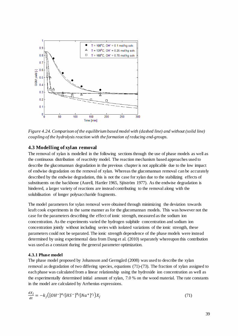
39
Figure 4.24. Comparison of the equilibrium based model with (dashed line) and without (solid line)
coupling of the hydrolysis reaction with the formation of reducing end-groups.
4.3 Modelling of xylan removal
The removal of xylan is modelled in the following sections through the use of phase models as well as
the continuous distribution of reactivity model. The reaction mechanism based approaches used to
describe the glucomannan degradation in the previous chapter is not applicable due to the low impact
of endwise degradation on the removal of xylan. Whereas the glucomannan removal can be accurately
described by the endwise degradation, this is not the case for xylan due to the stabilizing effects of
substituents on the backbone (Aurell, Hartler 1965, Sjöström 1977). As the endwise degradation is
hindered, a larger variety of reactions are instead contributing to the removal along with the
solubilisation of longer polysaccharide fragments.
The model parameters for xylan removal were obtained through minimizing the deviation towards
kraft cook experiments in the same manner as for the glucomannan models. This was however not the
case for the parameters describing the effect of ionic strength, measured as the sodium ion
concentration. As the experiments varied the hydrogen sulphide concentration and sodium ion
concentration jointly without including series with isolated variations of the ionic strength, these
parameters could not be separated. The ionic strength dependence of the phase models were instead
determined by using experimental data from Dang et al. (2010) separately whereupon this contribution
was used as a constant during the general parameter optimization.
4.3.1 Phase model
The phase model proposed by Johansson and Germgård (2008) was used to describe the xylan
removal as degradation of two differing species, equations (71)-(73). The fraction of xylan assigned to
each phase was calculated from a linear relationship using the hydroxide ion concentration as well as
the experimentally determined initial amount of xylan, 7.0 % on the wood material. The rate constants
in the model are calculated by Arrhenius expressions.
([
] [ ] [ ] ) (71)

40
[ ] (72)
(73)
The model was fitted against 195 kraft cook experiments, resulting in the parameters presented in table
4.5. When the native wood material was treated with cooking liquor at room temperature and an alkali
concentration of 1.25 mol OH-/kg liquor for 180 min, 95 % of the xylan remained insoluble (Wigell
2007). As for the modelling of glucomannan degradation, the initially soluble amount was omitted
from the modelling and experimental values exceeding this level excluded. The standard error of
estimation for the phase model was found to be 5.0 % with a coefficient of determination of 0.95.
Although the model described variations in cooking conditions satisfactory, see figures 4.25-4.27, the
model performance is deficient during the latter stages of the cook. This can be seen by studying the
residuals in figure 4.28. It should also be noted that the effect of cooking liquor composition during
the early stages if the cook is very small, indicating that the solubility of the polysaccharide fragments
removed in this stage is high.
Figure 4.25. The temperature dependence of the phase model with a liquor composition of OH
-=0.26
mol/kg solvent, HS-=0.26 mol/kg solvent, Na
+=0.52 mol/kg solvent.

41
Figure 4.26. The hydroxide ion dependence of the phase model at 168°C with a liquor composition of
HS-=0.26 mol/kg solvent and Na
+=0.52 mol/kg solvent.
Figure 4.27. The hydroxide ion dependence of the phase model at 168°C with a liquor composition of
OH-=0.26 mol/kg solvent and Na
+=0.52 mol/kg solvent.

42
Figure 4.28. Predictions of the phase model plotted against the experimental data.
Part of the model deviation for the phase model arises as a result of the changes in degradation rate
with decreasing yield being insufficient. This can be seen as there are two visible curvatures in figure
4.28. The modelled degradation rate is lower than the observed at yields in the range of 0.8-0.95 where
the initial phase dominates. The modelled degradation rate does however surpass the obsereved
degradation rate as the amount of xylan remaining in the initial phase decreases, resulting in a region
where the model predictions are lower than the experimental results. The same trend can also be
observed at the lower yields corresponding to the final xylan degradation phase. To account for these
apparent model deficiencies the model was modified by the addition of exponents to the amount of
xylan in each phase, resulting in the model being described by equation (74).
([
] [ ] [ ] )
(74)
The modified phase model had a significantly improved ability to describe the experimental data as
the standard error of estimation was determined to 3.4 % with a coefficient of determination of 0.97.
The improved model performance can be seen when studying the residuals in figure 4.29. The
residuals for the modified phase model are evenly distributed around the experimental values.
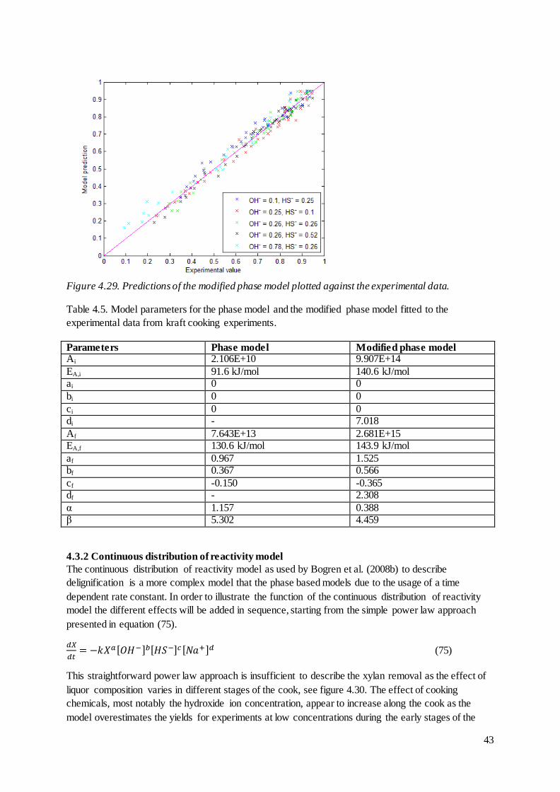
43
Figure 4.29. Predictions of the modified phase model plotted against the experimental data.
Table 4.5. Model parameters for the phase model and the modified phase model fitted to the
experimental data from kraft cooking experiments.
Parameters Phase model Modified phase model Ai 2.106E+10 9.907E+14
EA,i 91.6 kJ/mol 140.6 kJ/mol ai 0 0
bi 0 0
ci 0 0 di - 7.018
Af 7.643E+13 2.681E+15 EA,f 130.6 kJ/mol 143.9 kJ/mol
af 0.967 1.525 bf 0.367 0.566
cf -0.150 -0.365 df - 2.308
α 1.157 0.388 β 5.302 4.459
4.3.2 Continuous distribution of reactivity model
The continuous distribution of reactivity model as used by Bogren et al. (2008b) to describe
delignification is a more complex model that the phase based models due to the usage of a time
dependent rate constant. In order to illustrate the function of the continuous distribution of reactivity
model the different effects will be added in sequence, starting from the simple power law approach
presented in equation (75).
[ ] [ ] [ ] (75)
This straightforward power law approach is insufficient to describe the xylan removal as the effect of
liquor composition varies in different stages of the cook, see figure 4.30. The effect of cooking
chemicals, most notably the hydroxide ion concentration, appear to increase along the cook as the
model overestimates the yields for experiments at low concentrations during the early stages of the

44
cook whereas the yield at a high alkali level is overestimated during the latter stages. The standard
error of estimation for the power law model was determined to be 6.2 % for the power law model,
with a coefficient of determination of 0.92.
Figure 4.30. Predictions of the power law model plotted against the experimental data.
The varying effect of cooking chemicals may readily be accounted for in the power law model at the
cost of an increased number of parameters. A linear dependence on the xylan yield was added to the
power law model, see equation (76), increasing the number of parameters to 9. The model accuracy
was significantly improved by these additions as the standard error of estimation and the coefficient of
determination was found to be 4.9 % and 0.95 respectively. The model does however still yield
systematic error, as evident from the curvature in figure 4.31. The modelled degradation rate is higher
than the observed during a section in the middle of the xylan degradation, indicating that a relaxation
of the exponential decay may improve the model accuracy.
[ ] [ ] [ ] (76)

45
Figure 4.31. Residuals of the power law model with exponents describing the effect of cooking
chemicals linearly dependent on the xylan yield.
The continuous distribution of reactivity model is similar to the power law models with the addition of
relaxation of the exponential decay. This is achieved by the usage of a time-dependent rate constant
defined according to equation (77), yielding the model as described by equation (78).
( ) (77)
( ([ ] [ ] [ ] )
)
(
)
(78)
The relaxation factor, γ, has been found to be temperature dependent in studies of delignification
(Montané et al. 1994; Bogren et al. 2008b). As similar result where found in this study, the relaxation
factor was modelled as linearly dependent on the cooking temperature.
(79)
The continuous distribution of reactivity model decreased the systematic error of the model
predictions significantly, especially during the early stages of the cook, see figure 4.32. The standard
error of estimation was found to be 3.7 % with a coefficient of determination of 0.97.

46
Figure 4.32. Predictions of the continuous distribution of reactivity model plotted against the
experimental data.
Table 4.6. Model parameters for the power law models and the continuous distribution of reactivity
model when fitted to kraft cooking experiments.
Parameter Power law model Power law model,
varying exponents
CDR model
A 3.246E+11 5.224E+11 5.049E+17 EA 98.5 kJ/mol 107.1 kJ/mol 157.1 kJ/mol
a 5.158 1.179 - b1 1.091 3.910 3.893
b2 - -4.388 -4.162 c1 0.506 1.490 1.302
c2 - -1.611 -1.303 d1 -0.365 -0.840 -0.840
d2 - 0.950 0.950 γ1 - - -2.068
γ2 - - 6.62E-3

47
4.4 Validation of glucomannan models
The power law based model suggested by Wigell et al. (2007b) and the equilibrium based model
provided very similar descriptions of the glucomannan degradation in the evaluated interval of
cooking conditions, see figure 4.33. Both model types are thus equally able to describe this set of
experimental data. It is however important to not overestimate the significance of the model
parameters in the equilibrium based model as the used equilibrium constants is influenced by
additional effects that the model does not account for separately. The performance of both models is
validated in the following sections with experimental data from other authors using differing cooking
conditions. These validations provide information about the reliability of the respective models to
operate outside of the interval of cooking conditions for which they were optimized.
Figure 4.33. Comparison of the Wigell model (solid line), the Wigell model with hydrogen sulphide
dependence (dotted line) and the equilibrium based model (dashed line).
4.4.1 Validation using soda cooking experiments
The reliability of the models with parameters obtained through optimization towards the experimental
data from kraft cooks was investigated by comparison with cooking series from other authors. The 133
cooking experiments of Wigell et al. (2007a) was used for validation of the Wigell model and the
equilibrium based model at soda cooking conditions, see figures 4.34-4.37. Both models are able to
describe the effects of temperature and hydroxide ion concentration well, although the equilibrium
based model suggests lower differences between the alkali levels. The overall fit is however lacking as
the kraft cooking experiments resulted in lower hemicellulose yields than the soda cook experiments.

48
Figure 4.34. Validation of the Wigell model using soda cook experiments (Wigell et al. 2007a) with a
hydroxide ion concentration of 0.5 mol/kg solvent.
Figure 4.35. Validation of the Wigell model using soda cook experiments (Wigell et al. 2007a) with a
cooking temperature of 168°C.

49
Figure 4.36. Validation of the equilibrium based model using soda cook experiments (Wigell et al.
2007a) with a hydroxide ion concentration of 0.52 mol/kg solvent.
Figure 4.37. Validation of the equilibrium based model using soda cook experiments (Wigell et al.
2007a) with a cooking temperature of 168°C.
When studying the glucomannan degradation as a function of delignification, figure 4.38, it may be
suggested that the significantly decreased delignification obtained during soda cooking has a limiting
effect on the glucomannan degradation. The difference in delignification is far more pronounced
between the soda cook experiments and the kraft cook experiments than between the varying
concentrations of hydrogen sulphide among the kraft cook experiments. This implies that already low
hydrogen sulphide concentrations are sufficient to improve the delignification significantly, a
difference that in turn may result in increased glucomannan degradation. Studying the degradation
through alkaline hydrolysis separately through usage of wood material pretreated with sodium
borohydride reveals that the decreased glucomannan degradation at soda cooking condition originates
from a lower degree of primary peeling. This effect may be explained by increased physical stopping

50
as a result of lignin-carbohydrate complexes as the delignification is decreased, an effect that is most
prevalent during the rapid primary peeling.
Figure 4.38. Comparison of experimental data obtained from soda and kraft cooking experiments. The
liquor has a hydroxide ion concentration of 0.52 mol/kg solvent and the cooking temperatures are
139°C (Δ) and 168°C (○).
4.4.2 Validation using ionic strength experiments
Dang et al. (2010) studied the effect of ionic strength on kraft cooking kinetics using wood meal in a
flow through reactor. It was found that variations in ionic strength lacked significant impact on the
glucomannan degradation. The previously unpublished glucomannan yields from the 72 cooking
experiments are used in this thesis for model validation, see figure 4.39. The results are in good
agreement with the autoclave experiments used for parameter optimization as the standard error of
estimation for both the Wigell model and the equilibrium based model was determined to 4.2 % while
the standard error of estimation for the Wigell model with hydrogen sulphide dependence was 4.0 %.
The deviation between model and experimental data is a result of the slightly lower yield obtained in
the validation series than in the experimental data used for the modelling, a difference that is
illustrated in figure 4.40.
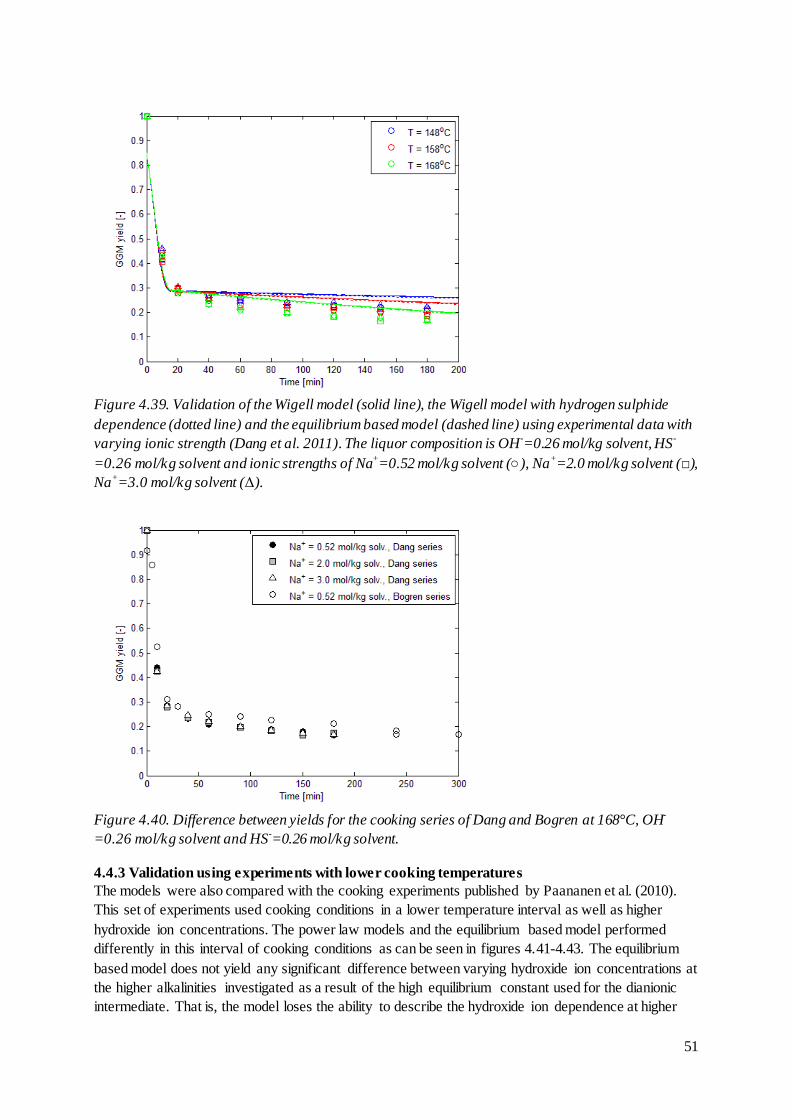
51
Figure 4.39. Validation of the Wigell model (solid line), the Wigell model with hydrogen sulphide
dependence (dotted line) and the equilibrium based model (dashed line) using experimental data with
varying ionic strength (Dang et al. 2011). The liquor composition is OH-=0.26 mol/kg solvent, HS
-
=0.26 mol/kg solvent and ionic strengths of Na+=0.52 mol/kg solvent (○), Na
+=2.0 mol/kg solvent (□),
Na+=3.0 mol/kg solvent (Δ).
Figure 4.40. Difference between yields for the cooking series of Dang and Bogren at 168°C, OH
-
=0.26 mol/kg solvent and HS-=0.26 mol/kg solvent.
4.4.3 Validation using experiments with lower cooking temperatures
The models were also compared with the cooking experiments published by Paananen et al. (2010).
This set of experiments used cooking conditions in a lower temperature interval as well as higher
hydroxide ion concentrations. The power law models and the equilibrium based model performed
differently in this interval of cooking conditions as can be seen in figures 4.41-4.43. The equilibrium
based model does not yield any significant difference between varying hydroxide ion concentrations at
the higher alkalinities investigated as a result of the high equilibrium constant used for the dianionic
intermediate. That is, the model loses the ability to describe the hydroxide ion dependence at higher

52
alkalinity. The Wigell model was however able to describe the trends rather well whereas the modified
Wigell model failed due to the joint increase of hydrogen sulphide concentration and hydroxide ion
concentration in the experiments. These two concentrations have opposite effects on the primary
peeling in the model which result in similar final yields, contrary to the experimental results. This is an
effect of the low cooking temperatures used as the delignification is limited during all the trails. As the
lignin removal is low regardless of the liquor composition the physical stopping through lignin-
carbohydrate complexes is maintained as the concentration of hydrogen sulphide is increased. The
effect of hydrogen sulphide concentration thus appear to be temperature dependent as the amount of
residual lignin is the affecting factor on glucomannan removal, not the actual concentration of
hydrogen sulphide. The hydrogen sulphide dependence could thus rather be included in an expression
accounting for the retaining effect of lignin-carbohydrate complexes.
Figure 4.41. Validation of the Wigell model using experimental data with a higher range of alkalinity
than the data used for optimization (Paananen et al. 2010). The cooking liquor has a sulphidity of
33 % and the cooking temperatures are 80°C (□), 105°C (○) and 130°C (Δ).
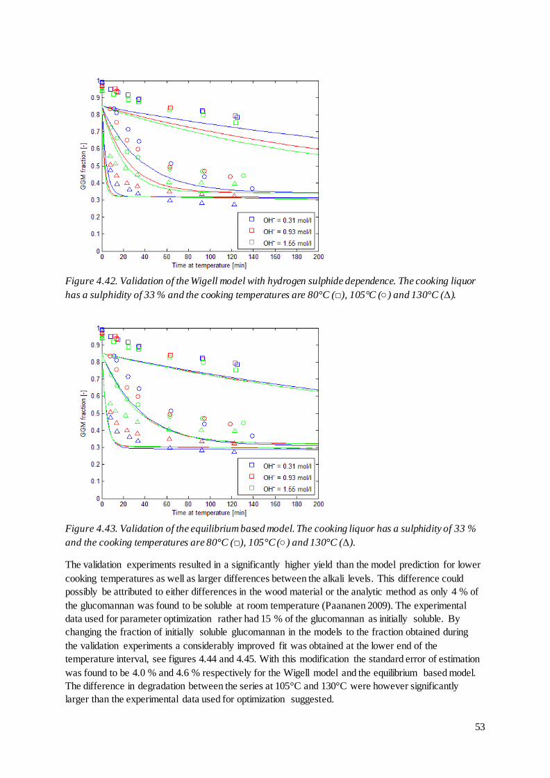
53
Figure 4.42. Validation of the Wigell model with hydrogen sulphide dependence. The cooking liquor
has a sulphidity of 33 % and the cooking temperatures are 80°C (□), 105°C (○) and 130°C (Δ).
Figure 4.43. Validation of the equilibrium based model. The cooking liquor has a sulphidity of 33 %
and the cooking temperatures are 80°C (□), 105°C (○) and 130°C (Δ).
The validation experiments resulted in a significantly higher yield than the model prediction for lower
cooking temperatures as well as larger differences between the alkali levels. This difference could
possibly be attributed to either differences in the wood material or the analytic method as only 4 % of
the glucomannan was found to be soluble at room temperature (Paananen 2009). The experimental
data used for parameter optimization rather had 15 % of the glucomannan as initially soluble. By
changing the fraction of initially soluble glucomannan in the models to the fraction obtained during
the validation experiments a considerably improved fit was obtained at the lower end of the
temperature interval, see figures 4.44 and 4.45. With this modification the standard error of estimation
was found to be 4.0 % and 4.6 % respectively for the Wigell model and the equilibrium based model.
The difference in degradation between the series at 105°C and 130°C were however significantly
larger than the experimental data used for optimization suggested.

54
Figure 4.44. Validation of the Wigell model when modified fraction of initially soluble material to
correspond with validation experiments. The cooking liquor has a sulphidity of 33 % and the cooking
temperatures are 80°C (□), 105°C (○) and 130°C (Δ).
Figure 4.45. Validation of the Wigell model with hydrogen sulphide dependence when modified
fraction of initially soluble material to correspond with validation experiments. The cooking liquor
has a sulphidity of 33 % and the cooking temperatures are 80°C (□), 105°C (□) and 130°C (Δ).
4.4.4 Validation at lower liquor to wood ratio
Bogren et al. (2009b) performed a series of validation trails without the high liquor to wood ratio
required in order to achieve constant composition cooks. The liquor to wood ratio in these trails was
7:1 and the experiments are thus similar to industrial conditions. The hydroxide ion concentration in
the cooking liquor decreased rapidly during the early stages of the cook as the more or less
instantaneous hydrolysis of acetyl groups as well as the primary peeling result in alkali consumption

55
(Chiang et al. 1987). The concentration of hydroxide ions was therefore measured during the cook and
the concentration profile included in the modelling.
The validation trails used liquors prepared from salts as well as industrial white liquor, industrial green
liquor and industrial black liquor, table 4.5. The degradation of glucomannan was not significantly
affected by the inactive ion composition of the liquors, see figure 4.38. This result is in agreement with
the results from Dang et al. (2011) suggesting that the glucomannan degradation is largely unaffected
by the ionic strength. The addition of dissolved wood components did however have a retarding effect
on the glucomannan degradation during the early stages of the cook.
The addition of dissolved wood components to the cooking liquor has been proposed to increase the
bulk delignification rate as well as the carbohydrate yield at a given kappa number, whereas the
delignification rate during the latter stages of the cook is impaired (Sjöblom 1996; Sjödahl et al. 2004).
The effect on delignification has however been shown to be dependent on the inactive ion composition
of the cooking liquor (Bogren et al. 2009a), while no such difference has been observed for the
hemicelluloses. It has been suggested that the carbohydrate yield increase largely is a result of xylan
sorption onto the fibres (Sjödahl et al. 2004), although the observed increase in glucomannan yield
indicates that additional effects contribute, see figure 46.
Table 4.5. Liquor composition for the validation trails using a liquor to wood ratio of 7:1.
Synt. WL 1 Synt. WL 2 WL BL/WL GL/WL
Na+ [mol/kg solv.] 1.04 1.2 1.26 2.28 2.83
K+ [mol/kg solv.] - - 0.07 0.14 0.13
OH- [mol/kg solv.] 0.89 0.90 0.90 1.01 0.98
HS- [mol/kg solv.] 0.15 0.30 0.15 0.17 0.37
CO32-
[mol/kg solv.]
- - 0.11 0.22 0.79
SO42-
[mol/kg solv.] - - 0.01 0.03 0.03
Cl- [mol/kg solv.] - - 0.01 0.03 0.02
Lignin [g/kg solv.] - - - 47.5 -
Figure 4.46. Glucomannan yield for the validation experiments at low liquor to wood ratio and a
cooking temperature of 160°C.

56
The model predictions ranged between the experimental results from the validation trails, see figure
4.47-4.49. The models were thus slightly overestimating the yields although the apparent effect of
dissolved wood components was unaccounted for. The standard errors of estimation was determined to
be 3.6 % and 3.3 % respectively for the Wigell model and the equilibrium based model as they both
described the validation trails similarly. The Wigell model with hydrogen sulphide dependence did
however yield an additional deviation as the validation trails did not result in any difference between
varying hydrogen sulphide concentrations. This result corresponds to the validation against the
experimental data published by Paananen et al. (2010) and it is thus likely that the effect of hydrogen
sulphide concentration on the glucomannan degradation noted in the experimental data used for model
optimization is overestimated. The standard error of estimation for the Wigell model with hydrogen
sulphide dependence was found to be 3.9 %.
Figure 4.47. Validation of the Wigell model at the industrially feasible liquor to wood ratio of 7 to 1.
Figure 4.48. Validation of the equilibrium based model at the industrially feasible liquor to wood ratio
of 7 to 1.

57
Figure 4.49. Validation of the Wigell model with hydrogen sulphide dependence at the industrially
feasible liquor to wood ratio of 7 to 1.
4.4.5 Validation with sodium borohydride addition
The contribution of the different degradation reactions to the glucomannan removal was validated by
cooking trails using wood material pretreated with sodium borohydride. As sodium borohydride is a
strong reducing agent it deactivates the end-groups and prevent primary peeling. The persisting
degradation is thus a result of alkaline hydrolysis and secondary peeling. At cooking temperatures
below 123°C the degradation was not significant as the yield after 3 hours remained about the initially
insoluble amount of 85 %. The degradation was however significant at elevated temperatures, see
figure 4.50, and the models described this degradation sufficiently. The standard error of estimation
for the 12 data points was found to be 4.0 % for the Wigell model and 4.5 % for the equilibrium based
model.

58
Figure 4.50. Validation of the alkaline hydrolysis and secondary peeling contribution with sodium
borohydride pretreated wood material. The cooking temperature was 168°C and the liquor had a
hydroxide ion concentration of 0.78 mol/kg solvent and were either soda cook or had a hydrogen
sulphide concentration of 0.26 mol/kg solvent. Wigell model (solid line), Equilibrium based model
(dashed line).
4.5 Validation of xylan models
When comparing the solutions of the phase models and the continuous distribution of reactivity model
it is important to note that the model structures are vastly different. This result in differing coupling of
the model parameters between the models and thus solutions that are not nearly as consistent as for the
models describing glucomannan degradation, see figure 4.51. This behaviour is illustrated by the
behaviour at low yields of the phase model modified to include exponents on the amount of xylan
remaining. The strong dependence on the xylan amount remaining decreases the degradation rate to a
higher extent at high alkalinities, the parameter coupling thus decreases the accuracy at low yields.
The performance of the phase models and the continuous distribution of reactivity model are validated
with experimental data from additional experimental series in the following sections. The effect of
ionic strength is however not validated as the experimental data series of Dang et al. (2010) were used
for parameter determination. The ionic strength series are however used for validation of the overall
degradation effect and temperature dependence.

59
Figure 4.51. Comparison of the continuous distribution of reactivity model (solid line), the phase
model (dotted line) and the phase model modified to contain exponents on the amount of xylan
remaining (dashed line).
4.5.1 Validation using ionic strength experiments
Flow through reactor experiments provided by Dang et al. (2010) was used for validation of the xylan
removal models as well as for determination of the parameters concerning the ionic strength
dependence. The experimental results from the flow through reactor and the autoclave experiments
used for model optimization differ during the early stages of the cook, figure 4.52, due to differences
in temperature profile. Using the temperature profile from the flow through reactor experiments does
however not sufficiently increase the rate of xylan removal, see figures 4.53-4.55, resulting in large
deviation between model and experiments during the heating up period. The difference between the
flow through reactor and the autoclave experiments are however limited to the early stages of the cook
as the final xylan yields are similar.
Figure 4.52. Experimental results at 168°C and a liquor composition of OH
-=0.26 mol/kg solvent and
HS-=0.26 mol/kg solvent for the flow through reactor (Dang series) and the autoclave experiments
(Bogren series).

60
The performance of the different models is illustrated in figures 4.53-4.55. The effects of ionic
strength variations are well described by all models as the flow through reactor experiments were used
for parameter determination. The standard error of estimations were calculated while only considering
cooking times exceeding 30 min, resulting in 64 used experimental data points. The continuous
distribution of reactivity model had the lowest standard error of estimation with 4.1 % whereas values
for the phase model and the modified phase were 6.3 % and 5.5 % respectively.
Figure 4.53. Ionic strength dependence and validation of the phase model towards experimental data
from a constant composition flow through reactor. The cooking temperature was 148°C (○) and
168°C (Δ) with a liquor composition of OH-=0.26 mol/kg solvent and HS
-=0.26 mol/kg solvent.
Figure 4.54. Ionic strength dependence and validation of the modified phase model towards
experimental data from a constant composition flow through reactor. The cooking temperature was
148°C (○) and 168°C (Δ) with a liquor composition of OH-=0.26 mol/kg solvent and HS
-=0.26 mol/kg
solvent.

61
Figure 4.55. Ionic strength dependence and validation of the continuous distribution of reactivity
model towards experimental data from a constant composition flow through reactor. The cooking
temperature was 148°C (○) and 168°C (Δ) with a liquor composition of OH-=0.26 mol/kg solvent and
HS-=0.26 mol/kg solvent.
4.5.2 Validation using experiments with lower cooking temperatures
The model behaviour at low cooking temperatures where investigated using the experimental data of
Paananen et al. (2010) in the temperature range of 80-130°C. Similar to the comparison with the
experimental data from the ionic strength investigation, the model performs poorly during the early
stages of the cook, plausibly due to the different temperature profiles used during the experimental
procedure as the time is corrected to time at cooking temperature. The phase models are able to
describe the rapid initial degradation to a higher extent than the continuous degradation of reactivity
model, they are however not functional at the lower end of the temperature interval, see figure 4.56-
4.58. The continuous distribution of reactivity model on the other hand is unable to account for the
different temperature profile due to the time dependence of the rate constant. The time dependence
requires that the model parameters are determined for a specific temperature profile, thus decreasing
the ability of the model to operate outside the conditions for which it is optimized.
Due to the large differences in these respective regions, the standard error of estimation is substantial
for the low cooking temperatures validation; 6.8 % for the continuous distribution of reactivity model,
10.7 % for the phase model and 8.4 % for the modified phase model. The effect of varying the cooking
chemical concentration is however well described by the modified phase model and the continuous
distribution of reactivity model in the hydroxide ion concentration range from 0.31-1.55 mol/l with a
constant sulphidity of 33 %.
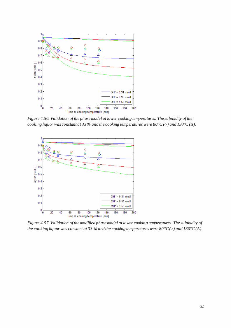
62
Figure 4.56. Validation of the phase model at lower cooking temperatures. The sulphidity of the
cooking liquor was constant at 33 % and the cooking temperatures were 80°C (○) and 130°C (Δ).
Figure 4.57. Validation of the modified phase model at lower cooking temperatures. The sulphidity of
the cooking liquor was constant at 33 % and the cooking temperatures were 80°C (○) and 130°C (Δ).

63
Figure 4.58. Validation of the continuous distribution of reactivity model at lower cooking
temperatures. The sulphidity of the cooking liquor was constant at 33 % and the cooking temperatures
were 80°C (○) and 130°C (Δ).
4.5.3 Validation at lower liquor to wood ratio
The validation series with the industrially feasible liquor to wood ratio of 7:1 performed by Bogren et
al. (2009b) was used for validation of the xylan removal models. Both cooking liquors prepared from
salts as well as industrial cooking liquors were included in these trails, see table 4.6. Only minor
differences were noticeable between the varying cooking liquors, with the largest difference arising
from the black liquor series, figure 4.59. The difference between the black liquor series and the other
cooking liquors is largest during the early sections of the cook whereas the final yields are similar. A
plausible explanation for this behaviour is that the dissolved wood components in the black liquor
decreases the solubility of xylan fragments, lowering the removal rate initially. As the degradation
proceeds in a non-constant composition cook, the amount of dissolved wood components builds up in
the cooking liquor and thus decreasing the relative influence of the initially added wood components.
Table 4.6. Liquor composition for the validation trails using a liquor to wood ratio of 7:1.
Synt. WL 1 Synt. WL 2 WL BL/WL GL/WL Na
+ [mol/kg solv.] 1.04 1.2 1.26 2.28 2.83
K+ [mol/kg solv.] - - 0.07 0.14 0.13
OH- [mol/kg solv.] 0.89 0.90 0.90 1.01 0.98
HS- [mol/kg solv.] 0.15 0.30 0.15 0.17 0.37
CO32-
[mol/kg solv.]
- - 0.11 0.22 0.79
SO42-
[mol/kg solv.] - - 0.01 0.03 0.03
Cl- [mol/kg solv.] - - 0.01 0.03 0.02
Lignin [g/kg solv.] - - - 47.5 -

64
Figure 4.59. Validation series with varying cooking liquors, both industrial and synthetic, at a liquor
to wood ratio of 7:1 and a cooking temperature of 160°C.
The model performance of the phase models are negatively influenced by the hydroxide ion
dependence of the phase composition. The initial consumption of hydroxide ions is large due to
primary peeling as well as hydrolysis of acetyl groups (Chiang et al. 1987) and the concentration thus
drops significantly in cooks with lower liquor to wood ratios. The initial phase xylan is thus
overestimated and the model deviates during the early stages of the cook, see figure 4.60 and figure
4.61. The main deviation between the validation trails and the models are however located during the
latter stages of the cook. The models consistently presents lower yields than the experimental data, an
effect that may be explained by the accumulation of dissolved wood components in the cooking liquor
resulting in lowered solubility. The standard error of estimation for the phase model, the modified
phase model and the continuous distribution of reactivity model was found to be 10.0 %, 6.9 % and
6.1 % respectively.
Figure 4.60. Validation of the phase model using various cooking liquors at a liquor to wood ratio of
7:1 and a cooking temperature of 160°C.

65
Figure 4.61. Validation of the modified phase model using various cooking liquors at a liquor to wood
ratio of 7:1 and a cooking temperature of 160°C.
Figure 4.62. Validation of the continuous distribution of reactivity model using various cooking
liquors at a liquor to wood ratio of 7:1 and a cooking temperature of 160°C.
66
5. Conclusions The following conclusions have been reached through the modelling work presented in this thesis:
- The glucomannan losses during kraft pulping can be accurately described by models based on
the main reaction mechanisms involved. However, additional parameters describing the
physical stopping of the endwise degradation is required to expand the applicability to a wider
range of cooking conditions.
- The glucomannan yield is higher in soda cook experiments than in kraft cooking experiments.
This indicates that the decreased delignification has a retaining effect, possibly through lignin-
carbohydrate linkages. The glucomannan degradation was however not largely affected by
changes in hydrogen sulphide concentration among the kraft cooking experiments as the effect
on degree of delignification was far less pronounced.
- The removal of xylan is largely controlled by the dissolution of longer polysaccharide
fragments due to the stabilizing effect of substituents on the endwise degradation. A reaction
mechanism based approach to describing the removal is thus unsuitable.
- An increased ionic strength lowers the solubility of xylan. The xylan removal is however
increased by addition of NaHS, indicating a strong correlation between delignification and
xylan removal. The lignin-carbohydrate linkages can be supposed to influence the retention of
xylan to a larger extent than glucomannan due to a closer affinity to lignin. The dissolution
limited xylan removal also increases the effect, whereas glucomannan largely is degraded to
monomers.

67
Acknowledgements This master thesis was performed within the framework of Avancell - Centre of Fibre Engineering. I
would like to thank the following people for making it possible:
- Professor Hans Theliander, my advisor and examiner, for encouragement and support.
- Dr. Harald Brelid, my co-supervisor, for arranging this project and being an unlimited source
of ideas and knowledge.
- Dr. Johannes Bogren, M.Sc. Binh Dang, Dr. Anna Saltberg and Lic. Alexandra Wigell for
providing the experimental data that this thesis is based upon.
I would also like to thank everyone at the Division of Forest Products and Chemical Engineering and
Chemical Environmental Science at Chalmers, you all make it a terrific working environment.
Finally I would like to thank my friends, my family and Augusta, for their support and above all; for
putting up with me.

68
References Andersson, N. (2003) Modelling of kraft cooking kinetics using near infrared spectroscopy, Diss.
Karlstad University Studies, Karlstad, Sweden.
Andersson, N., Wilson, D. I., Germgård, U. (2003) An improved kinetic model structure for softwood
kraft pulping, Nordic Pulp & Paper Res. J. 18(2), 200-209.
Aurell, R., Hartler, N. (1965) Kraft pulping of pine, Part 1. The changes in the composition of the
wood residue during the cooking process, Svensk Papperstidn. 68(3), 59-68.
Bamford, C. H., Collins, J. R. (1950) Kinetic studies on carbohydrates in alkaline conditions. I. The
kinetics of the autoxidation of glucose, Proceedings of the Royal Society of London, Series A:
Mathematical, Physical and Engineering Sciences, 204, 62-84.
Bogren, J. (2008) Further insights into kraft cooking kinetics, Diss. Chalmers University of
Technology, Göteborg, Sweden.
Bogren, J., Brelid, H., Theliander, H. (2007) Reaction kinetics of softwood kraft delignification –
General considerations and experimental data, Nordic Pulp & Paper Res. J. 22(2), 177-183.
Bogren, J., Brelid, H., Theliander, H. (2008a) Effect of Pulping Conditions on the Rates of Formation
and Degradation of Hexenuronic Acid in Scots Pine, Journal of Pulp and Paper Science 34(1), 23-29.
Bogren, J. Brelid, H., Theliander, H. (2008b) Assessment of reaction kinetic models describing
delignification fitted to well-defined kraft cooking data, Nordic Pulp & Paper Res. J. 23(2), 210-217.
Bogren, J., Brelid, H., Bialik, M. Theliander, H. (2009a) Impact of dissolved sodium salts on kraft
cooking reactions, Holzforschung, 63(2), 226-231.
Bogren, J., Brelid, H., Theliander, H. (2009b) Towards a general kraft delignification model, Nordic
Pulp & Paper Res. J. 24(1), 33-37.
Chiang, V. L., Cho, J. L., Puumala, R. J., Eckert, R. E., Fuller, W. S. (1987) Alkali consumption
during kraft pulping of Douglas-fir, western hemlock and red alder, Tappi 70(2), 101-104.
Christensen, T., Albright, L. F., Williams, T. J. (1983) A kinetic mathematical model for the kraft
pulping of wood, in: Tappi Annual Meeting, 239-243, Atlanta, Georgia, USA.
Christensen, J. J., Rytting, J. H., Izatt, R. M. (1970) Thermodynamics of proton dissociation in dilute
aqueous solution. Part XV. Proton dissociation from several monosaccharides at 10 and 40°C, J.
Chem. Soc. Section B, (9), 1646-1648.
Dang, B., Brelid, H., Theliander, H. (2010) The effect of ionic strength on the kinetics of the kraft
pulping of softwood, 11th
Europan Workshop on Lignocellulosics and Pulp, 313-316.
Dang, B., Brelid, H., Bogren, J., Theliander, H. (2011) Different sodium ion concentration profiles
during kraft cooking- impact on the delignification and carbohydrate removal, 16th
ISWFPC, 641-645.
Franzon, O., Samuelson, O. (1957) Degradation of cellulose by alkali cooking, Svensk Papperstidn.
60(23), 872-877.

69
Gellerstedt, G. (2008) Chapter 20 Chemistry of pulping, The Ljungberg Textbook: Cellulose
Technology, Chalmers University of Technology, Göteborg.
Gustafson, R. R., Slelcher, C. A., McKean, W. T., Finlayson, B. A. (1983) Theoretical model of the
kraft pulping process, Ind. Eng. Chem. Process Des. Dev., 22(1), 87-96.
Gustafsson, L., Teder, A. (1969) Alkalinity in alkaline pulping, Svensk Papperstidn. 72(24), 795-801.
Gustavsson, C., Al-Dajani, W. W. (2000) The influence of cooking conditions on the degradation of
hexenuronic acid, xylan, glucomannan and cellulose during kraft pulping of softwood, Nordic Pulp &
Paper Res. J. 15(2), 160-167.
Hansson, J., Hartler, N. (1968) Alkaline degradation of Xylans from Birch and Pine, Svensk
Papperstidn. 71(9), 358-365.
Hansson, J., Hartler, N. (1969) Sorption of Hemicelluloses on Cellulose Fibres. Part 1. Sorption of
Xylans, Svensk Papperstidn. 72(17), 521-530.
Jacobs, A., Dahlman, O. (2001) Characterization of the molar masses of hemicelluloses from wood
and pulps employing size exclusion chromatography and matrix-assisted laser desorption ionization
time-of-flight mass spectrometry. Biomacromolecules 2(3), 894-905.
Johansson, D. (2008) Carbohydrate degradation and dissolution during Kraft cooking, Lic. Eng.
Thesis, Karlstad University Studies, Karlstad, Sweden.
Johansson, D., Germgård, U. (2008) Carbohydrate degradation during softwood kraft cooking –
influence on cellulose viscosity, carbohydrate composition and hexenuronic acid content, Nordic Pulp
& Paper Res. J. 23(3), 292-298.
Johansson, D., Germgård, U. (2007) A kinetic study of softwood Kraft cooking – carbohydrate
dissolution as a function of cooking conditions, Appita Journal, 61(3), 228-233.
Lai, Y. Z. (1981) Kinetics of base-catalyzed cleavage of glycosidic linkages, in: Ekman-Days, Int.
Symp. Wood Pulping Chem., 2, 26-33.
Lai, Y. Z., Sarkanen K. V. (1969) Kinetic study on the alkaline degradation of amylose, J. Polym. Sci.,
Part C, 28:15-26.
Lawoko, M., Henriksson, G., Gellerstedt, G. (2005) Structural Differences between the Lignin-
Carbohydrate Complexes Present in Wood and in Chemical Pulps, Biomacromolecules, 6, 3467-3473.
Lémon, S., Teder, A. (1973) Kinetics of the delignification in Kraft pulping, Svensk Papperstidn.
76(11), 407-414.
Lindgren, C. T., Lindström, M. E. (1996) The Kinetics of Residual Delignification and Factors
Affecting the Amount of Residual Lignin During Kraft Pulping, Nordic Pulp & Paper Res. J. 12(2),
124-127, 134.
Mitikka-Eklund, M. (1996) Sorption of xylans on cellulose fibers, Lic. Eng. Thesis, University of
Jyväskylä, Jyväskylä, Finland.

70
Montané, D., Overend, R.P., Chornet, E. (1998) Kinetic Models for Non-Homogeneous Complex
Systems With a Time-Dependent Rate Constant, Canadian Journal of Chemical Engineering 76(1),
58-68.
Montané, D., Salvadó, J., Farriol, X., Jollez, P., Chornet, E. (1994) Phenomenological kinetics of
wood delignification: Application of a time dependent rate constant and a generalized severity
parameter to pulping and correlation of pulp properties, Wood Science and Technology 28(6), 387-
402.
Motomura, H., Bae, S.-H., Morita, Z. (1998) Dissociation of hydroxyl groups of cellulose at low ionic
strengths, Dyes and Pigments, 39(4), 243-258.
Neale, S. M. (1930) The swelling of cellulose and its affinity relations with aqueous solutions. II. Acid
properties of regenerated cellulose illustrated by absorption of sodium hydroxide and water from
dilute solutions, and the consequent swelling, Journal of the Textile Institute, 21, 225-230.
Norgren, M., Edlund, H., Wågberg, L. Annerggren, G. (2002) Fundamental physical aspects on lignin
dissolution, Nordic Pulp & Paper Res. J. 17(4), 370-373.
Norgren, M., Lindström, B. (2000) Dissociation of phenolic groups in kraft lignin at elevated
temperatures, Holzforschung, 54, 519-527.
Olofsson, G., Hepler, L. G. (1975) Thermodynamics of Ionization of Water over Wide Ranges of
Temperature and Pressure, Journal of Solution Chemistry, 4(2), 127-143.
Paananen, M. (2009) Degradation kinetics of softwood carbohydrates during alkaline cooking with
emphasis on the peeling-stopping reaction, M.Sc. Thesis, Helsinki University of Technology,
Helsinki, Finland.
Paananen, M., Tamminen, T., Nieminen, K., Sixta, H. (2010) Galactoglucomannan stabilization
during the initial kraft cooking of Scots pine, Holzforschung, 64, 683-692.
Plonka, A. (1986) Time-Dependent Reactivity of Species in Condensed Media, Lecture Notes in
Chemistry, Springer, Berlin.
Procter, A. R., Apelt, H. M. (1969) Reactions of wood components with hydrogen sulfice. III.
Efficiency of hydrogen sulfide pretreatment compared to other methods for stabilizing cellulose to
alkaline degradation, Tappi 52(8), 1518-1522.
Pu, Q., McKean, W., Gustafson, R. (1991) Kinetic model of softwood kraft pulping and simulation of
the RDH process, Appita, 44(6):399-404.
Pu, Q., Sarkanen, K. (1991) Donnan equilibria in wood-alkali interactions. Part 2. Effect of
polysaccharide ionization at high alkalinities, Journal of Wood Chemistry and Technology 11(1), 1-
22.
Ralph, J.,Lundquist, K., Brunow, G., Lu, F., Kim, H., Schatz, P. F., Marita, J. M., Hatfield, R. D.,
Ralph, S. A., Christensen, J. H., Boerjan, W. (2004) Lignins: Natural polymers from oxidative
coupling of 4-hydroxyphenylpropanoids, Phytochemistry Reviews 3(1-2), 29-60.

71
Ribe, E., Lindblad Söderqvist-Lindblad, M., Dahlman, O., Theliander, H. (2010) Xylan sorption
kinetics at industrial conditions - Part 1. Experimental results, Nordic Pulp & Paper Res. J. 25(2), 138-
149.
Sartori, J.,Potthast, A., Rosenau, T., Hofinger, A., Sixta, H., Kosma, P. (2004) Alkaline degradation of
model compounds related to beech xylan, Holzforschung, 58, 588-596.
Simonson, R. (1963) The Hemicellulose in the Sulfate Pulping Process. Part 1. The Isolation of
Hemicellulose Fractions from Pine Sulfate Cooking liquors, Svensk Papperstidn. 66(20), 839-845.
Simonson, R. (1965) The Hemicellulose in the Sulfate Pulping Process. Part 3. The Isolation of
Hemicellulose Fractions from Birch Sulfate Cooking liquors, Svensk Papperstidn. 68(8), 275-280.
Sjöblom, K. (1996) Extended delignification in kraft cooking through improved selectivity. Part 5.
Influence of dissolved lignin on the rate of delignification, Nordic pulp & Paper Res. J. 11(3), 177-
185.
Sjödahl, R. G., Ek, M., Lindström, M. E. (2004) The effect of sodium ion concentration and dissolved
wood components on the kraft pulping of softwood, Nordic pulp & Paper Res. J. 19(3), 325-329.
Sjöström, E. (1977) The behavior of wood polysaccharides during alkaline pulping processes, Tappi
60(9), 151-154.
Sjöström, E. (1993) Wood Chemistry: Fundamentals and Applications, second edition, Academic
Press, San Diego, California, USA.
Sjöström, E., Westermark, U. (1999) Chemical compositions of wood and pulps: basic constituents
and their distribution, in: Analytical methods in wood chemistry, pulping and papermaking, Sjöström,
E., Alén, R., (eds.) p. 3., Springer, Berlin.
Smith, C. C., Williams, T. J. (1974) Mathematical modelling, simulation and control of the operation
of a Kamyr continuous digester for the kraft process, Technical Report 54, Purdue University.
Teder, A., Olm, L. (1981) Extended delignification by combination of modified kraft pulping and
oxygen bleaching, Paperi ja Puu 63(4a), 315-318, 321-322, 325-326.
Teder, A., Tormund, D. (1981) Equilibria in pulping and bleaching liquors, in: Ekman-Days, Int.
Symp. Wood Pulping Chem., 5, 108-111.
Whistler, R.L., BeMiller, J.N. (1958) Alkaline degradation of polysaccharides, Advances in
carbohydrate chemistry, 13, 289-329.
Wigell, A. (2007) Reaction kinetics of hemicellulose: Modelling yield loss during alkaline cooking of
softwood meal, Lic. Eng. Thesis, Chalmers University of Technology, Göteborg, Sweden.
Wigell, A., Brelid, H., Theliander H. (2007a) Degradation/dissolution of softwood hemicellulose
during alkaline cooking at different temperatures and alkali concentrations, Nordic Pulp & Paper Res.
J. 22(4), 488-494.
Wigell, A., Brelid, H., Theliander, H. (2007b) Kinetic modelling of (galacto)glucomannan degradation
during alkaline cooking of softwood, Nordic Pulp & Paper Res. J. 22(4), 495-499.

72
Wilson,G., Procter, A. R. (1970) Reactions of wood components with hydrogen sulfide: Part V. The
kinetics of kraft and soda delignification of western hemlock, Pulp and Paper Magazine of Canada
71(22), T483-T487.
Yllner, S., Enström, B. (1956) Studies on the adsorption of xylan on the cellulose fibres during the
sulphate cook, Part I, Svensk Papperstidn. 59(6), 229-232.
Young, R. A., Liss, L. (1978) A kinetic study of the endwise degradation of gluco- and
galactomannans, Cellul. Chem. Technol. 12:399-411.
Young, R. A., Sarkanen, K. V., Johnson, P. G., Allan, G.G. (1972) Marine plant polymers, Part III,
Kinetic analysis of the alkaline degradation of polysaccharides with specific reference to (1,3)-β-D-
glucans, Carbohyd. Res. 21:111-122.