modelling of failure in high strength steel sheets

Linkoping Studies in Science and TechnologyThesis No. 1529

Modelling of Failurein High Strength Steel Sheets

Oscar Bjorklund

LIU–TEK–LIC–2012:14

Department of Management and Engineering, Division of Solid MechanicsLinkoping University,

SE–581 83, Linkoping, Swedenhttp://www.solid.iei.liu.se/

Linkoping, April 2012

Cover:Results from finite element simulation of a forming limit test.

Printed by:LiU-Tryck, Linkoping, Sweden, 2012ISBN 978–91–7519–895–5ISSN 0280–7971

Distributed by:Linkoping UniversityDepartment of Management and EngineeringSE–581 83, Linkoping, Sweden

c© 2012 Oscar BjorklundThis document was prepared with LATEX, April 30, 2012

No part of this publication may be reproduced, stored in a retrieval system, or betransmitted, in any form or by any means, electronic, mechanical, photocopying,recording, or otherwise, without prior permission of the author.

Preface

The work presented in this thesis has been carried out at the Division of SolidMechanics, Linkoping University with financial support from the VINOVA PFFproject ”Fail” and the SFS ProViking project ”SuperLight Steel Structures”. Theindustrial partners Dynamore Nordic, Outokumpu Stainless, Saab Automobile,Scania, SSAB, SvereaIVF and Volvo Car Corporation are also gratefully acknowl-edged for their support.

I would like to thank my supervisor, Professor Larsgunnar Nilsson for all his sup-port and guidance during course of this work. I also greatly appreciate all mycolleagues at the Division of Solid Mechanics for their help, in particular RikardLarsson, Lic. Eng., for all his support and guidance concerning constitutive mod-elling.

For their assistance during the mechanical testing throughout this project I wouldlike to thank Andreas Lundstedt at Outokumpu Stainless and Bo Skoog, UlfBengtsson and Soren Hoff at Linkoping University.

I am also grateful to all my friends and my family for their support over the courseof all these years. I could not have done it without you.

Oscar Bjorklund

Linkoping, April 2012

”Results! Why, man, I have gotten a lot of results. I know several thousand thingsthat won’t work”

Thomas Edison

iii

Abstract

In this theses the high strength steel Docol 600DP and the ultra high strength steelDocol 1200M are studied. Constitutive laws and failure models are calibrated andverified by the use of experiments and numerical simulations. For the constitu-tive equations, an eight parameter high exponent yield surface has been adopted,representing the anisotropic behaviour, and a mixed isotropic-kinematic hardeninghas been used to capture non-linear strain paths.

For ductile sheet metals three different failure phenomena have been observed: (i)ductile fracture, (ii) shear fracture, and (iii) instability with localised necking. Themodels for describing the different failure types have been chosen with an attemptto use just a few tests in addition to these used for the constitutive model. In thiswork the ductile and shear fracture have been prescribed by models presented byCockroft-Latham and Bressan-Williams, respectively. The instability phenomenonis described by the constitutive law and the finite element models. The resultsobtained are in general in good agreement with test results.

The thesis is divided into two main parts. The background, theoretical framework,mechanical experiments and finite element models are presented in the first part.In the second part, two papers are appended.

v

List of Papers

In this thesis, the following papers have been included:

I. R. Larsson, O. Bjorklund, L. Nilsson, K. Simonsson (2011). A study ofhigh strength steels undergoing non-linear strain paths - Experiments andmodelling, Journal of Materials Processing Technology, Volume 211, pp. 122-132.

II. O. Bjorklund, R. Larsson, L. Nilsson (2012). Failure of high strength steelsheets - Experiments and modelling, Submitted.

Own contribution

In the first paper, Rikard Larsson and I jointly performed the modelling and ex-perimental work. However, Rikard Larsson was responsible for writing the paper.In the second paper, the modelling and experimental work were once again per-formed by Rikard Larsson and myself, but I was responsible for evaluating thefailure phenomena and for writing the paper.

vii

Contents

Preface iii

Abstract v

List of Papers vii

Contents ix

Part I Theory and Background

1 Introduction 3

2 Steels 52.1 Crystal Structure . . . . . . . . . . . . . . . . . . . . . . . . . . . . 62.2 Dual Phase Steel . . . . . . . . . . . . . . . . . . . . . . . . . . . . 62.3 Martensitic Steel . . . . . . . . . . . . . . . . . . . . . . . . . . . . 7

3 Deformation and Fracture 9

4 Constitutive Modelling 114.1 Isotropic Hardening . . . . . . . . . . . . . . . . . . . . . . . . . . . 124.2 Kinematic Hardening . . . . . . . . . . . . . . . . . . . . . . . . . . 144.3 Mixed Hardening . . . . . . . . . . . . . . . . . . . . . . . . . . . . 154.4 Effective Stress . . . . . . . . . . . . . . . . . . . . . . . . . . . . . 16

5 Fracture Modelling 195.1 Ductile Fracture . . . . . . . . . . . . . . . . . . . . . . . . . . . . . 225.2 Shear Fracture . . . . . . . . . . . . . . . . . . . . . . . . . . . . . 235.3 Phenomenological Fracture Models . . . . . . . . . . . . . . . . . . 23

6 Modelling Instability 296.1 Instability in Plane Strain . . . . . . . . . . . . . . . . . . . . . . . 296.2 Analytical Instability Models . . . . . . . . . . . . . . . . . . . . . 316.3 The Marciniak and Kuczynski Model . . . . . . . . . . . . . . . . . 336.4 Finite Element Model . . . . . . . . . . . . . . . . . . . . . . . . . . 35

ix

6.5 Evaluation of Instability . . . . . . . . . . . . . . . . . . . . . . . . 36

7 Mechanical Experiments 397.1 Pre-Deformation . . . . . . . . . . . . . . . . . . . . . . . . . . . . 397.2 Tensile Test . . . . . . . . . . . . . . . . . . . . . . . . . . . . . . . 417.3 Simple Shear Test . . . . . . . . . . . . . . . . . . . . . . . . . . . . 417.4 Plane Strain Test . . . . . . . . . . . . . . . . . . . . . . . . . . . . 427.5 Balanced Biaxial Test . . . . . . . . . . . . . . . . . . . . . . . . . . 427.6 Nakajima Test . . . . . . . . . . . . . . . . . . . . . . . . . . . . . . 43

8 Finite Element Modelling 458.1 Pre-Straining . . . . . . . . . . . . . . . . . . . . . . . . . . . . . . 468.2 Tensile Test . . . . . . . . . . . . . . . . . . . . . . . . . . . . . . . 468.3 Shear Test . . . . . . . . . . . . . . . . . . . . . . . . . . . . . . . . 478.4 Plane Strain Test . . . . . . . . . . . . . . . . . . . . . . . . . . . . 488.5 Nakajima Test . . . . . . . . . . . . . . . . . . . . . . . . . . . . . . 50

9 Conclusions and Discussion 51

10 Review of Appended Papers 53

Bibliography 55

Part II Appended Papers

Paper I: A study of high strength steels undergoing non-linear strainpaths - Experiments and modelling . . . . . . . . . . . . . . . . . . 63

Paper II: Failure of high strength steel sheets - Experiments and modelling 77

x

Part I

Theory and Background

Introduction1

Due to the desire from industries to shorten product development lead time, theuse of Simulation Based Design (SBD) is rapidly increasing. The development offinite element (FE) methods and the rapid growth of computational power havemade it possible for SBD to advance from research to industrial utilisation. Inaddition to reduced development time and cost, the possibility of determining theproduct’s properties at an early stages of the design process is of utmost impor-tance e.g. to find out if a car is safe in a crash situation. Simultaneously withthe development of SBD, material suppliers have developed more advanced steelswith improved mechanical properties. However, these advanced steels often showanisotropic behaviour and more complex hardening compared to traditional low-carbon steels. Consequently, the demand for research on material models, includingfailure models suitable for these steels, has increased.

The constitutive model that has been used throughout this work includes an eightparameter high exponent yield surface with mixed isotropic-kinematic hardening.The model has the ability to represent the anisotropic behaviour that is shown inmechanical tests, even for a complex loading path. To further increase the abilityto predict the product’s potential and thereby enable a more optimised product,the necessity of improving failure models has arisen. At present, progressive fail-ure is not included in automotive FE simulations. In order to predict the likeli-hood of failure, the predicted strain states are compared to experimental forminglimit curves (FLC). However, the experimental FLC is constructed for linear strainpaths, although its locus has been shown to depend on the strain path. Therefore,the prediction of failure of a component, e.g. a car body part subjected to a crashsimulation, lacks information from its previous design history. Thus, an improvedphenomenological model for prediction of failure is desired. A phenomenologicalfailure model must have the ability to inherit the properties of a component fromits prior manufacturing process.

Macroscopic fractures have always been of great interest. As early as the beginningof 16th century, Leonardo da Vinci explained fractures in terms of mechanicalvariables. He established that the load an iron wire could carry depended on thelength of the wire, as a consequence of the amount of voids in the material. Thelonger the wire, the more voids, which led to lower load-carrying capacity. Evenif material fracture has been studied for a long time, the underlying microscopicalfracture mechanisms are hard to translate to a phenomenological model. Since the

3

CHAPTER 1. INTRODUCTION

underlying mechanisms need to be represented on a length scale, which can be usedin an FE simulation, it would be computationally expensive, and hence too timeconsuming, to represent the fracture on a micromechanical scale. Throughout thiswork, the expressions failure and fracture are used extensively:

• Failure - loss of load-carrying capacity of a component or a structure.

• Fracture - material separation into two, or more, pieces.

The term failure incorporates the term fracture but may also be other structuralphenomena which do not include a material separation, e.g. material and geometri-cal instabilities. In ductile sheet metals three different failure phenomena have beenobserved: (i) ductile fracture, (ii) shear fracture and (iii) material instability withlocalisation. The third term instability with localisation is also sometimes denotedas purely-plastic failure. In this work the different phenomena have been modelledseparately and the focus has been placed on using failure models which can easilybe calibrated from simple mechanical tests. For modelling of the ductile and shearfractures the Cockroft-Latham and Bressan-Williams models, respectively, havebeen used. Each of their models contains only one material parameter and areeasy to calibrate. The instability phenomenon is described by the FE model andthe constitutive law and needs no further mechanical experimental calibration.

Even if the objective of this project is to identify improved material and failuremodels suited for high strength sheet metals, the benefit in a longer perspectivemay be the opportunity to produce lighter and safer structures. The environmentalprofit of producing lighter products is obvious for the automotive industry, but alsoother industrial applications can profit from reducing weight i.e. lighter containerswill result in an ability to increase the pay-load. The safety of occupants in carshas been an increasingly important marketing issue for the automotive industry.By using new materials to the very edge a more optimised product can be obtainedand thereby many fatalities may be prevented.

4

Steels2

The classification of different steel grades is often made by the amount and typeof alloying substances. However, it is also common to talk about different groupsof steels, e.g. High-Strength Low Alloy (HSLA) steel, High-Strength Steel (HSS),Ultra High-Strength Steel (UHSS), Advance High-Strength Steel (AHSS), DualPhase (DP) Steel, and Transformation-Induced Plasticity (TRIP) Steel. A specificsteel can be a part of more than one group as there is no unequivocal division.However, in this work the materials studied are categorised into the two groupsHSS and UHSS. These groups are grouped according to the yield strength, andsteels with a yield strength between 210 to 550 MPa are classified as HSS andsteels with a yield strength over 550 MPa are classified as UHSS, see Opbroek(2009).

The steels covered in this study are Docol 600DP and Docol 1200M. The name Do-col is a SSAB trademark. Docol 600DP is an HSS with a dual face structure consist-ing of about 75% ferrite and 25% martensite, where the two-phase microstructureis produced by heat treatment. Docol 1200M is an UHSS with a fully martensiticsteel produced by water quenching from an elevated temperature in the austeniticrange, see Olsson et al. (2006). The nominal thicknesses of the steel sheets studiedwere 1.48 mm and 1.46 mm for Docol 600DP and Docol 1200M, respectively. Fordetails on the chemical composition of the Docol 600DP and Docol 1200M, seeTable 1.

Table 1: Chemical composition of Docol 600DP and Docol 1200M.

C Si Mn P S Nb Al Fe

[%] [%] [%] [%] [%] [%] [%] [%]

Docol 600DP 0.10 0.20 1.5 0.01 0.002 - 0.04 balance

Docol 1200M 0.11 0.2 1.6 0.015 0.002 0.015 0.04 balance

5

CHAPTER 2. STEELS

2.1 Crystal Structure

The crystal structure of the atoms in a metal is composed of regular three dimen-sional patterns called a crystal lattice. There are a number of different types ofcrystal lattices and it is common to talk about unit cells of different types. Formetals, the most common types of unit cells are body-centered cubic (BCC), face-centered cubic (FCC), hexagonal close-packed (HCP), and body-centered tetrago-nal (BCT), see Figure 1. For a more complete overview of different types of unitcells see e.g. Askeland (1998). For pure iron there are three different types ofphases called α, γ and δ. The α-iron, also known as ferrite, is present at temper-atures up to 912C and has a BCC phase structure. Between 912C and 1394Cthe pure iron is known as γ-iron, or austenite, which has an FCC phase structure.Above 1394C and up to the melting point at 1538C the iron is known as δ-iron,or delta ferrite, which also has a BCC phase structure. By adding carbon or otheralloying elements the range of the different phases will be altered, for more detailedinformation see e.g. Krauss (2005). By controlled cooling of the metal, the phasescan be prevented from changing, thereby a phase which is present under high tem-peratures can be obtained at room temperature. However, also new phases suchas martensite can be obtained by rapidly cooling austenite.

(a) BCC (b) FCC (c) HCP

$

1 ,

'((

'(

)((

#

(d) BCT

Figure 1: Different types of unit cells common for metals, (a) body-centered cubic,(b) face-centered cubic, (c) hexagonal close-packed and (d) body-centered tetragonal.

2.2 Dual Phase Steel

Dual phase steels mainly consist of ferrite and a minor part of martensitic secondphase particles. The second phase particles can be seen as channels and darkerareas between the ferritic islands in Figure 2(a). An increase of the amount of hardmartensitic particles generally increases strength and reduces ductility. The dualphase is produced either by controlled cooling from the austenitic phase or fromthe ferrite-austenite phase. The carbon (C) enables the formation of martensite atpractical cooling rates. By adding other alloying element such as manganese (Mn),

6

2.3. MARTENSITIC STEEL

chromium (Cr), molybdenum (Mo), vanadium (V) and nickel (Ni) individually orin combination, an increase in the hardenability of the steel can be obtained.

2.3 Martensitic Steel

Martensitic steels are produced by a quenching from a temperature in the austeniticrange. The steels are characterised by a martensitic matrix with small parts of fer-rite or bainite. The martensite can be seen as small needle shaped particles inFigure 2(b). The hardenability can be increased by adding carbon (C) or other al-loying elements such as manganese (Mn), silicon (Si), chromium (Cr), molybdenum(Mo), boron (B), vanadium (V) and nickel (Ni).

(a)

(b)

Figure 2: Microstructure for: (a) Docol 600DP and (b) Docol 1200M.

7

Deformation and Fracture3

The deformation of steel can be divided into elastic and inelastic parts. The elastic(reversible) deformation, which occurs at the atomic level, does not cause any per-manent deformation of the material. Inelastic or plastic deformation, on the otherhand, causes permanent deformation. This deformation occurs within the crystalstructure by a procedure known as slip. The slip produces crystal defects, calleddislocations, and when the deformation continues a large number of these defectsoccurs. The dislocations in the crystal lattice cause obstacles, which prevent themobility of subsequent dislocations and thereby contribute to a hardening mech-anism. Elastic or plastic deformations do not destroy the atomic arrangement ofthe material while fractures, on the other hand, cause discontinuities within thematerial. These discontinuities cause stress concentrations which will increase the’rate’ of fracturing. There are two main types of fracture: brittle and ductile.

Brittle fracture is the breaking of interatomic bonds without noticeable plastic de-formation. These fractures occur when the local strain energy becomes larger thanthe energy necessary to pull the atom layers apart. Brittle fracture occurs mainlyin high-strength metals with poor ductility and toughness. However, even metalsthat have normal ductility may exhibit brittle fracture at low temperatures, inthick sections or at high strain-rates. The surface of a brittle fracture is charac-terised by its flat appearance and the fracture surface is most often perpendicularto the applied load.

Ductile fracture, on the other hand, is caused by an instability which is the resultof very extensive plastic deformations occurring in the surroundings of crystallinedefects. The global deformation in a ductile fracture may be either large or small,depending on the density of the defects. The ductile fracture is described as theinitiation, growth and coalescence of voids in the material, and finally the loadedarea has been reduced and the material fails. The surface of the ductile fracture ischaracterised by the presence of shear lips, which results in the form of a cup anda cone on the two fracture surfaces. It is also often possible to see the dimples thatare caused by the micro-voids. The material examined in this study is assumedto fail only in a ductile manner, and consequently the brittle fracture type is notconsidered.

9

CHAPTER 3. DEFORMATION AND FRACTURE

In ductile sheet metals or thin walled structures, failure can be caused by oneor a combination of the following; (i) ductile fracture, (ii) shear fracture or (iii)instability with localisation, see Figure 3.

(a) (b)

) *+ !

4 #$ "

!

(c)

Figure 3: Failure types in sheet metals, (a) ductile fracture, (b) shear fracture, (c)instability with localisation.

The ductile fracture arises since most materials contain inclusions or particles, andduring deformation voids are likely to nucleate at these locations. Further plasticdeformation will cause them to grow until they link together to produce a ductilefracture. Hydrostatic tension will increase the volume of the voids and therebyfavours this type of fracture.

Shear fracture can be caused either by extensive slip on the activated slip planes,see Dieter (1986), or as a result of void nucleation in the slip bands. Both of thesemechanisms are favoured by shear stresses. When voids nucleate in the slip bands,the loaded area is reduced such that plastic flow localises there. Continued shearincreases the area of the voids until separation occurs. Furthermore, as stated byTeirlinck et al. (1988) ”Voids which extend in shear need not increase in volume, soshear fracture is less pressure-dependent than ductile fracture, though it remainsmore pressure-dependent than purely-plastic failure”.

Instability or plastic failure occurs if no other mechanism intervenes. In the ordi-nary tensile test of a sheet metal sample two types of instability can occur: diffusenecking and localised necking. Both mechanisms occur when the strain hardeningcan no longer compensate for the increased load. Diffuse necking in a tensile testoccurs as a reduction of the waist over a length which has about the same sizeas the width of the waist. Localised necking takes place inside the diffuse zoneas a thickness reduction along a narrow band which has about the same size asthe thickness. In a more general loading case, localisation can occur without apreceding diffuse necking. Since the strain localises inside the neck the materialfails there due to ductile or shear fracture.

10

Constitutive Modelling4

In order to be able to formulate the hypothesis on which the constitutive modelsare based, it is necessary to understand the basic physical deformation mechanismsof the material as described in Chapter 3. Since applications in sheet metal formingand vehicle collision involve large deformations and rotations of the material, it isnecessary to formulate the constitutive equations in a consistent manner. By usinga co-rotational material framework, see e.g. Belytschko et al. (2000), these largedeformations and rotations can be accounted for. The co-rotated Cauchy stresstensor can the be expressed as

σ = RTσR (1)

where R is the orthogonal transformation tensor and σ denotes the co-rotatedCauchy stress tensor, σ. From now on (·) denotes the co-rotated quantity of(·). The co-rotated rate of deformation tensor is assumed to follow an additivedecomposition of the elastic and plastic parts

D = De

+ Dp

(2)

where superscript e and p denotes elastic and plastic parts, respectively. In casesof small elastic deformations, a hypo-elastic stress update can be assumed, i.e.

˙σ = C : (D − Dp) (3)

where C is the co-rotated fourth order elastic stiffness tensor. Henceforth, theco-rotated superscript, (·), will be excluded and all subsequent relations will berelated to co-rotated configuration. Plastic deformation will not occur as long asthe stress state is considered as elastic. Whether or not the stress state is in theelastic regime is determine by the yield function, f

f = σ − σyiso (4)

11

CHAPTER 4. CONSTITUTIVE MODELLING

where σ is the effective stress and σyiso is the current yield stress. The yield functiondetermines the elastic limit of the material and the hypersurface, when f = 0 isdenoted as the yield surface. As long as f < 0 no plastic deformations will occurand when f = 0 and f = 0 plastic flow will occur. The plastic part of the rate ofdeformation tensor will be determined from the plastic potential, g, according to

Dp = λ∂g

∂σ(5)

where λ is the plastic multiplier and the gradient of g determines in which directionthe material will flow. In an associated, in contrast to a non-associated, flowrule the flow is directed normal to the yield surface and in that case the plasticpotential and the yield function coincide, i.e. g = f . This, assumption has beenused throughout this work. Three different modes of loading can occur, (i) elasticcase then λ = 0 and f < 0, (ii) plastic loading λ ≥ 0 and f = 0 , and (iii)neutral loading if the direction of loading is tangential to the yield surface λ = 0and f = 0. These three cases may be expressed using the Karush-Kuhn-Tuckerconditions (KKT-conditions).

λ ≥ 0, f ≤ 0, λf = 0 (6)

4.1 Isotropic Hardening

As discussed earlier, plastic deformation is caused by dislocations in the materialand the growth of these dislocations will prevent the mobility of new ones andthereby increase the stress that is necessary to produce an increased plastic strain.Most models for describing the current yield stress σyiso are given as functions ofthe equivalent plastic strain εp defined as

εp =

t∫

0

˙εpdt (7)

where t is the time. However, other quantities, e.g. the plastic strain-rate andtemperature, may also affect the hardening of the material. A large amount ofanalytic functions for describing the hardening can be found in literature. It hasalso been quite common to use the experimental hardening curves directly. Thetensile test is often used for describing hardening up to diffuse necking after whichsome kind of extrapolation is needed. In this work, an extended Voce law, see Voce(1948), was fitted to the hardening data from the tensile test up to diffuse necking.

12

4.1. ISOTROPIC HARDENING

After diffused necking an extrapolation using the Hollomon law (see Hollomon(1945)) i.e. a power-law, was adopted by the use of inverse modelling of a sheartest. The analytic hardening function can be expressed as

σyiso(εp) =

σ0 +2∑

i=1

QRi(1− e−CRiεp

) εp ≤ εt

A+B(εp)C εp > εt

(8)

where σ0, QRi, CRi, A, B and C are material constants and εt is the transitionpoint between the extended Voce and Hollomon hardening. The requirements ofa smooth curve, i.e. a C1 transition between the Voce and Hollomon expressions,makes it possible to determine the constants A, B and C with only one new pa-rameter denoted σ′100, which can be interpreted as the stress at 100% plastic strain.

A+B(εt)C = σ0 +2∑

i=1

QRi(1− e−CRiεt

)

CB(εt)C−1 =2∑

i=1

CRiQRie−CRiε

t

A+B = σ′100

(9)

The isotropic hardening can be illustrated as an expansion of the yield surface inall directions, see Figure 4(a).

σ1

σ2

!

" !

σ1

σ2

!

" !

σ1

σ2

σ1

σ2

σ1

σ2

#

(a)

σ1

σ2

!

" !

σ1

σ2

!

" !

σ1

σ2

σ1

σ2

σ1

σ2

#

(b)

σ1

σ2

!

" !

σ1

σ2

!

" !

σ1

σ2

σ1

σ2

σ1

σ2

#

(c)

Figure 4: Different types of hardening (a) isotropic, (b) kinematic and (c) mixed.

13


4.2 Kinematic Hardening

Plastic deformation may also introduce anisotropic behaviour of the material, e.g.as manifested by the Bauschinger effect, which is the phenomenon of a lower yieldstress in the case of reverse loading. For modelling this effect it is useful to introducea kinematic hardening model. The kinematic hardening enables the yield surfaceto move in the stress space, see Figure 4(b), and thereby obtain a reduced yieldstress in the case of reverse loading, see Figure 5.

, -%

Σ = σ −α &

α =

2∑

i=1

αi =

2∑

i=1

CXi

(QXi

Σ

σ−αi

)&

σ

ε

σRD

σTD

!

%

Figure 5: Ilustraition of the Bauschinger effect in the case of reverse loading.

The motion of the yield surface is described by the backstress tensor, α. Therelated overstress tensor, Σ = σ −α, replaces the Cauchy stress tensor, σ, in theeffective stress function, σ = σ(σ−α). An interpretation can be seen in Figure 6.

Σ = σ −α *

α =

2∑

i=1

αi =

2∑

i=1

CXi

(QXi

Σ

σ−αi

)-

σTD

σRDα

σΣ

.

Figure 6: Interpretation of the overstress, Σ, backstress, α, and Cauchy stresstensor, σ.

In this work the evolution of the backstress has been described by a two-componentlaw, presented by Frederick and Armstrong (2007)

14

4.3. MIXED HARDENING

α =2∑

i=1

αi =2∑

i=1

CXi

(QXi

Σ

σ−αi

)(10)

where QXi and CXi are material constants determined from pre-strained tensiletests.

4.3 Mixed Hardening

Throughout this work a combination of isotropic and kinematic hardening hasbeen used, i.e. the yield surface can both expand and move, see Figure 4(c). In thespecial case of uniaxial tension in the φ-direction the only non-zero componentsin the overstress, backstress, and Cauchy stress tensors will be Σφ, αφ, and σφ,respectively. The evolution of the backstress can then be expressed as

αφ(εp) = rφ

2∑

i=1

QXi(1− e−CXiεp

) (11)

where rφ = Σyφ/σ is constant and αφ(0) = 0 has been used. The yield stress, σyφ,

can now be expressed as a function of the equivalent plastic strain, εp.

σyφ(εp) = rφ

σ0 +2∑

i=1

[QRi(1− e−CRiε

p

) +QXi(1− e−CXiεp

)]εp ≤ εt

A+B(εp)C +2∑

i=1

QXi(1− e−CXiεp

) εp > εt(12)

As can be seen from Equation 12, the mixed hardening may, in the special caseof monotonic loading, be interpreted as a summation of isotropic and kinematichardening, see Figure 7. The total stress at 100% plastic strain, σ100, can now beexpressed as the function of the isotropic stress at 100% plastic strain, σ′100, andthe saturation of the kinematic hardening.

σ100 = σ′100 +2∑

i=1

QXi (13)

15


0 0.2 0.4 0.6 0.8 10

200

400

600

800

1000Str

ess,

σ[M

Pa]

Equivalent plastic strain, εp [-]

σy

σyisoα

εt

σ′100

σ100

Figure 7: Hardening decomposition in the case of monotonic loading.

In order to simplify the parameter identification procedure, a linear mixture be-tween the isotropic and kinematic hardening has been assumed according to

QRi = (1− βi)Qi, QXi = βiQi, i = 1, 2CRi = CXi = Ci, i = 1, 2

(14)

where βi determines the amount of kinematic hardening, and is restricted to avalue between 0 and 0.9 in order to avoid infeasible values of Ci.

4.4 Effective Stress

Many expressions for effective stress have been presented over the years. Theexpression for the effective stress according to von Mises is well known and oftenused. However, since the von Mises expression only shows isotropic behaviour, andsince the rolling process used for producing sheet metals usually leads to differentproperties in different directions, an anisotropic effective stress function is needed.The rolling direction (RD), transversal direction (TD) and normal direction (ND)are often used to describe the axes of orthotropy. Anisotropy can occur both inthe yield stress and in the plastic flow. The anisotropy in plastic flow is describedby the Lankford parameter, R, see e.g. Hosford and Cadell (1993), or the plasticstrain ratios, k, defined as

16

4.4. EFFECTIVE STRESS

Rφ =dεpTdεpN

, kφ =dεpTdεpL

=−Rφ

Rφ + 1(15)

where the indices on the logarithmic plastic strain increment indicate the transver-sal, T , normal N , and longitudinal, L, direction, respectively. The anisotropy inyield stress is described by

rφ =σyφσref

(16)

where σyφ is the yield stress in the φ direction and σref is a reference yield stress.Equations 15 and 16 are expressed for the tensile test case but similar equationscan be obtained for the balanced biaxial test

Rb = kb =dεpTDdεpRD

, rb =σybσref

(17)

where the subscript b denotes balance biaxial test. The interpretation of the plasticstrain ratios, k, and the yield stress ratios, r, are shown in Figure 8.

σTD

σRD

kb

1

(rbσref , rbσref )

k00

1

(0, r90σref )k90

1

(r00σref , 0)

Figure 8: Yield locus for a plane stress case with τRD = 0.

17


Expressions for representing anisotropic behaviour have been presented by numer-ous authors and a good overview is given in Banabic et al. (2010). In the presentstudy the model presented by Aretz (2005) has been used

σ(Σ) =

[1

2(|∆′1|a + |∆′2|a + |∆′′1 −∆′′2|a)

]1/a

(18)

∆′1∆′2

=A8Σ∗11 + A1Σ∗22

2±√(

A2Σ∗11 − A3Σ∗22

2

)2

+ A24Σ12Σ21 (19)

∆′′1∆′′2

=

Σ∗11 + Σ∗22

2±√(

A5Σ∗11 − A6Σ∗22

2

)2

+ A27Σ12Σ21 (20)

where A1, ..., A8 and a are material constants. The model was originally derived fora plane stress case, where the 11-direction and 22-direction correspond to the RDand TD, respectively. However, a regularisation that enables a C0 continuous thick-ness across the element edges has been carried out. Thus the through-thicknessnormal stress has been included in the effective stress measures, Σ∗11 = Σ11 − Σ33

and Σ∗22 = Σ22 − Σ33, where the 33-direction corresponds to the ND of the sheet.The identification of the parameters has been implemented both by direct methods,using the strain and stress ratios, and inverse modelling of the shear test.

18

Fracture Modelling5

Fracture can generally be divided into ductile and brittle fracture, as mentioned inChapter 3. The ductile fracture is categorised by a considerable amount of plasticdeformation prior to material separation. The brittle fracture, on the other hand,occurs at small or no plastic deformation. However, the steels examined in thisstudy are considered as ductile, therefore only this type of fracture will be consid-ered. From a micromechanical point of view the ductile fracture is characterisedby nucleation, growth and coalescence of voids in the material until finally theload-bearing area has been reduced and material separation occurs. The reductionin load-bearing area due to voids will lead to material softening. In damage me-chanics this effect is described as damage accumulation affecting the constitutivebehaviour and the models presented by Gurson (1977) and Lemaitre (1985) aretwo examples of such models. One simple way to consider this damage is proposedby Lemaitre and Chaboche (1990), given as a relationship between the initial andthe damaged area in a certain direction, see Figure 9.

Figure 9: Initial area, S, and damaged area, SD, in the normal direction, n.

The damage variable, Dn, can then be interpreted as the relationship between thedamaged area, SD, and the initial area, S, respectively.

Dn =SDS

(21)

In this definition of damage, ultimate fracture is expected when Dn reaches thevalue of 1, i.e. when the entire surface is damaged and there is no material left to

19

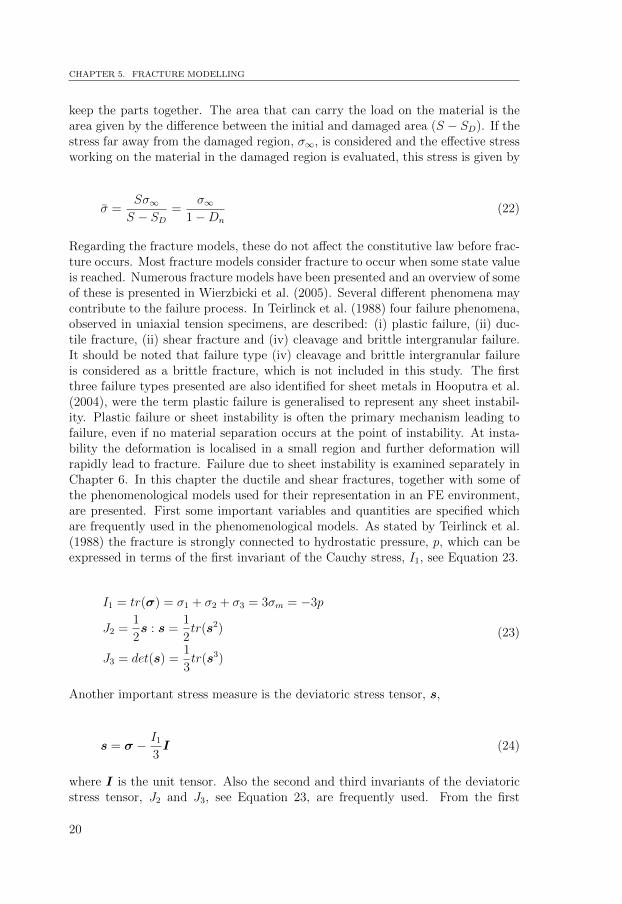
CHAPTER 5. FRACTURE MODELLING

keep the parts together. The area that can carry the load on the material is thearea given by the difference between the initial and damaged area (S − SD). If thestress far away from the damaged region, σ∞, is considered and the effective stressworking on the material in the damaged region is evaluated, this stress is given by

σ =Sσ∞S − SD

=σ∞

1−Dn

(22)

Regarding the fracture models, these do not affect the constitutive law before frac-ture occurs. Most fracture models consider fracture to occur when some state valueis reached. Numerous fracture models have been presented and an overview of someof these is presented in Wierzbicki et al. (2005). Several different phenomena maycontribute to the failure process. In Teirlinck et al. (1988) four failure phenomena,observed in uniaxial tension specimens, are described: (i) plastic failure, (ii) duc-tile fracture, (ii) shear fracture and (iv) cleavage and brittle intergranular failure.It should be noted that failure type (iv) cleavage and brittle intergranular failureis considered as a brittle fracture, which is not included in this study. The firstthree failure types presented are also identified for sheet metals in Hooputra et al.(2004), were the term plastic failure is generalised to represent any sheet instabil-ity. Plastic failure or sheet instability is often the primary mechanism leading tofailure, even if no material separation occurs at the point of instability. At insta-bility the deformation is localised in a small region and further deformation willrapidly lead to fracture. Failure due to sheet instability is examined separately inChapter 6. In this chapter the ductile and shear fractures, together with some ofthe phenomenological models used for their representation in an FE environment,are presented. First some important variables and quantities are specified whichare frequently used in the phenomenological models. As stated by Teirlinck et al.(1988) the fracture is strongly connected to hydrostatic pressure, p, which can beexpressed in terms of the first invariant of the Cauchy stress, I1, see Equation 23.

I1 = tr(σ) = σ1 + σ2 + σ3 = 3σm = −3p

J2 =1

2s : s =

1

2tr(s2)

J3 = det(s) =1

3tr(s3)

(23)

Another important stress measure is the deviatoric stress tensor, s,

s = σ − I1

3I (24)

where I is the unit tensor. Also the second and third invariants of the deviatoricstress tensor, J2 and J3, see Equation 23, are frequently used. From the first

20

invariants of the Cauchy stress, I1, the second and third invariants of the deviatoricstress, J2 and J3, the Haigh-Westergaard coordinates, ξ, ρ and θ can be defined

ξ =1√3I1

ρ =√

2J2 = σvM

cos(3θ) =

√27

3

J3

J3/22

(25)

where σvM is the equivalent von Mises stress. These coordinates can be explainedfrom Figure 10, where the ξ-axis is aligned with the hydrostatic axis (σ1 = σ2 = σ3),ρ-axis is the radius of the von Mises cylinder and θ is the Lode angle, cf. alsoFigure 11. The point B in the principal stress space can now be defined in theHaigh-Westergaard coordinates as

σ1

σ2

σ3

=

ξ√3

111

+

√2

3ρ

cos(θ)cos(θ − 2π/3)cos(θ + 2π/3)

(26)

σ1

σ2

σ3

O

σ1=σ2

=σ3

π,

ξ

ρA

O′Bθ

'

Figure 10: Von Mises cylinder shown in the principal Cauchy stress space.

21


σ1 σ2

σ3

A

B

θ

Figure 11: Von Mises cylinder shown in the π-plane.

The importance of the Lode angle, θ, on fracture has been reported, e.g. by Baiand Wierzbicki (2008). Also the importance of the stress triaxiality, η, which is therelationship between hydrostatic pressure and the equivalent von Mises stress, seeEquation 27, has been demonstrated by several authors e.g. Oyane et al. (1980)and Bao and Wierzbicki (2004).

η = − p

σvM(27)

5.1 Ductile Fracture

Even if the fracture models do not affect the elasto-plastic or elasto-viscoplasticconstitutive laws and thus produce a material softening, it is useful to considerthem as a type of growing function. One useful representation is

εf∫

0

F (state variables)dεp ≤ C (28)

where the function, F , may depend on any state variable and is integrated onthe effective plastic strain, εp. The state variables can be divided into observablevariables, e.g. temperature, T , total strain, ε, or internal, e.g. plastic strain, εp, orstress state, σ, among others. The simplest form of Equation 28 is when F ≡ 1, inwhich case the model predicts the equivalent plastic strain to fracture. However, afracture criterion given by constant equivalent plastic strain to fracture is contraryto experimental observations.

22

5.2. SHEAR FRACTURE

5.2 Shear Fracture

Shear fracture is a result of extensive slip on the activated slip planes. Consequentlythis fracture is favoured by shear stresses. The shear fracture can also be foundunder certain conditions when voids nucleate in the slip band and reduce the load-bearing area, so that continuous plastic flow localises there. Since sheet metalapplications often are modelled by shell elements, which most often are restrictedto plane stress assumptions, it is necessary to construct a fracture model that canpredict fracture due to transversal shear.

5.3 Phenomenological Fracture Models

A short review of some of the phenomenological fracture models presented in lit-erature is given below.

The Cockroft and Latham Criterion

Cockroft and Latham (1968) suggested a criterion based on an accumulated stressand plastic strain. More precisely they argued that the plastic work must be animportant factor for the fracture. The total amount of plastic work done per unitvolume at the fracture point is

W p =

εf∫

0

σdεp (29)

where σ is the current equivalent stress (σ = σyiso), εf is the fracture strain, and εp

the equivalent plastic strain. However, the current stress σ, unlike the peak stressσ1, is not influenced by the shape of the necked region. A criterion based on thetotal amount of plastic work will therefore predict a fracture independent of thisshape, which is contrary to experiments. Therefore, the total amount of plasticwork cannot provide a good criterion by itself, since necking is important accordingto experimental observations. A more reasonable fracture criterion would be to takethe magnitude of the highest tensile stress into account. Therefore, Cockroft andLatham proposed that fracture occurs in a ductile material when

W =

εf∫

0

σ(< σ1 >

σ

)dεp (30)

23


reaches a critical value, Wc, for a given temperature and strain rate. The non-dimensional stress concentration factor,

(<σ1>σ

), represents the effect of the highest

tensile stress, < σ1 >= max(σ1, 0). The reduced form

W =

εf∫

0

< σ1 > dεp ≤ Wc (31)

is used for the fracture evaluation, and fracture is expected when the integralreaches a critical value, Wc, which is determined from experiments. The Cockroftand Latham model implies that fracture in a ductile material depends both on thestresses and plastic strain states, i.e. neither stress nor strain alone can describeductile fracture. The benefit of using the largest principal stress, σ1, is that it canbe expressed as a function of the hydrostatic pressure, p, the second invariant ofthe deviator stress, J2 and the Lode angle, θ, as

σ1 = −p+

√4J2

3cos θ (32)

The Wilkins Criterion

The model by Wilkins et al. (1980), also known as the RcDc model, states thattwo factors increase the fracture threshold: the hydrostatic stress and the asym-metric stress. The hydrostatic stress accounts for the growth of holes by spalling.Interrupted tension tests have shown initiation and growth of voids which forma fracture surface. The asymmetric stress accounts for the observation that theelongation at fracture decreases as the shear load increases in fracture tests withcombined stress loads. The accumulated damage is expressed as

D =

εf∫

0

ω1 ω2 dεp ≤ 1 (33)

and the weight factors for the hydrostatic stress and the asymmetric stress areexpressed as

ω1 =

(1

1− C3σm

)C1

, ω2 = (2− AD)C2 (34)

24

5.3. PHENOMENOLOGICAL FRACTURE MODELS

where ω1 is the hydrostatic pressure weight, ω2 is the asymmetric stress weight, dεp

is the equivalent plastic strain increment, σm is the hydrostatic pressure and C1,C2, and C3 are material constants. The parameter AD included in the asymmetricstress weight, ω2 is defined as

AD = min

(∣∣∣∣s2

s3

∣∣∣∣ ,∣∣∣∣s2

s1

∣∣∣∣)

(35)

where s1, s2 and s3 are the principal stress deviators. The parameter AD rangesfrom 0 to 1, and when AD = 1 the stress field is symmetric (and asymmetric whenAD = 0). Fracture is expected when the damage parameter, D, in Equation 33reaches 1.

The Oyane Criterion

Oyane et al. (1980) suggested a fracture model to consider the effect of stresstriaxiality on ductile fracture. The model is derived from the plasticity theory forporous media as

εf∫

0

(C1 + η) dεp ≤ C2 (36)

where C1 and C2 are material constants and η is the stress triaxiality.

The Johnson and Cook Criterion

The fracture model presented by Johnson and Cook (1985) is a purely phenomeno-logical model, which is based on a similar relation as the hardening model presentedby Johnson and Cook (1983). The model uses a damage parameter D, and whenthis parameter reaches the value of 1, ultimate fracture is expected. The definitionof the damage parameter is

D =

εf∫

0

1

Φdεp ≤ 1 (37)

where εf is the equivalent strain to fracture and dεp is the increment of equivalentplastic strain. The expression for the function Φ is given as

Φ =(C1 + C2e

−C3η) [

1 + C4 ln

(˙εp

ε0

)](1 + C5T ) (38)

25


where C1, ..., C5 are material constants, which can be determined from experiments,η is the stress triaxiality, ˙εp is the equivalent plastic strain-rate, ε0 is a referencestrain-rate and T is the temperature. As noted from the Equations 37 and 38 themodel depends on strain, strain-rate, temperature and stress triaxiality.

The Bressan and Williams Criterion

Shell elements are often used for modelling sheet metal applications, but are fre-quently restricted to plane stress conditions. Thus, they are not able to describetransversal shear stresses. It is therefore necessary to consider a fracture criterionwhich can be used to predict this phenomenon. Bressan and Williams (1983) sug-gested a model for predicting instability through the thickness of a sheet metal.They suggested that the plastic strain increment should be equal to zero at an in-clined direction through the thickness of the sheet, i.e. dεpt = 0 in the et-directionshown in Figure 12. By assuming that the directions of the principal stress andstrains coincide, and by using the stress and strain tensor components accordingto Equation 39, together with the rotation tensor to rotate the stress and strainsto the incline directions (en, e2, et),

. *+

4 *+ ,$

et

en

e1

e2

e3

θ

$ %

dεpt = sin2 θ dεp1 + cos2 θ dεp3 = 0 &'

cos 2θ =dεp1 + dεp3dεp1 − dεp3

&)

cos 2θ =−dεp2

2dεp1 + dεp2= − β

2 + β&3

τnt = cosθsinθ(σ1 − σ3) = sin2θ(σ1 − σ3)

2&4

τnt =σ1 − σ3

2

√1 − (

β

2 + β)2 ≤ τc ':

:

Figure 12: Inclined plane through the thickness of the sheet. The stress and strainon the et-plane is determined from the values in the coordinate axis ei, wherei = 1...3, and the angle, θ.

σ =

σ1 0 00 σ2 00 0 0

, dεp =

dεp1 0 00 dεp2 00 0 dεp3

(39)

the strain increment in the et-direction and the shear stress on the inclined surfacecan be found as

26

5.3. PHENOMENOLOGICAL FRACTURE MODELS

dεpt = sin2 θdεp1 + cos2 θdεp3 = 0 (40)

and

σtn = −(σ1) sin θ cos θ (41)

Assuming that fracture occurs when the shear stress, σtn, on the inclined surfacereach a critical value τc, and that the material is plastically incompressible, thefollowing is obtained

cos 2θ =−dεp2

2dεp1 + dεp2=−β

2 + β(42)

and

sin 2θ = −2τcσ1

(43)

Here β = dεp2/dεp1 is the relationship between the in-plane principal plastic strains

and τc is a material constant. From Equations 42 and 43 the following inequalitycan be obtained

τ =σ1

2

√1−

( −β2 + β

)2

≤ τc (44)

where σ1/2 is the shear stress on the inclined surface, cf. Figure 12. As long asthe inequality is fulfilled no fracture is expected due to through-thickness shear.However, in this work a normal stress through the thickness has been introduced toobtain C0 continuity over the element edges. Therefore, the criterion in Equation 44is modified such that

τ =σ1 − σND

2

√1−

( −β2 + β

)2

≤ τc (45)

where σND is the through-thickness normal stress, and thus (σ1 − σND)/2 is theshear stress on the inclined surface.

27


The Han and Kim Criterion

Han and Kim (2003) suggested a criterion for ductile fracture, which combinesthe model by Cockcroft-Latham with a maximum shear stress criterion and thethrough thickness strain. Thus,

εf∫

0

< σ1 > dεp + C1(σ1 − σ3)/2 + C2εt ≤ C3 (46)

where C1, C2, and C3 are material parameters, determined from experiments, andεt is the thickness strain. Here it has been used so that the principal stresses followsσ1 > σ2 > σ3. Then the term (σ1 − σ3)/2 is the maximum shear stress.

28

Modelling Instability6

Even if there is no material separation during an instability, it is most often consid-ered as a limit of the operational use of the product. At instability the deformationis localised as a narrow band of the same width as the thickness of the sheet, seee.g. Dieter (1986). Due to the localisation, further deformation will rapidly leadto a material fracture. The prediction of instability limits is therefore importantin order to find the correct failure behaviour.

6.1 Instability in Plane Strain

The instability limit can, for the special case of plane strain, be derived analytically.However, the elastic strains are neglected here and all strains are assumed to beplastic. Consider a rod with a length, l, width, w, and thickness, t. The forcein the length direction can be expressed as F11 = σ11wt, where the subscript 11corresponds to the length direction. The instability arises when the force reachesa maximum viz. dF11 = 0. In terms of stress and strains, the following is obtained

dσ11

dεp11

= σ11 (47)

where dll

= dεp11, dww

= dεp22 = 0 (plane strain), dtt

= dεp33, has been used and thefact that the material is assumed to be plastically incompressible, i.e. dεp11 +dεp22 +dεp33 = 0. By assuming a plane stress assumption, the stress and strain componentscan be expressed as

ε = εp11

1 0 00 0 00 0 −1

, σ = σ11

1 0 00 γ 00 0 0

(48)

where γ is the stress ratio producing plane strain deformation, see Figure 13.

29

CHAPTER 6. MODELLING INSTABILITY

*+$,-+

⎡⎢⎢⎢⎣

σ1

σ2

σ3

⎤⎥⎥⎥⎦ =

ξ√3

+

√2

3ρ

⎡⎢⎢⎢⎣

cos(θ)

cos(θ − 2π/3)

cos(θ + 2π/3)

⎤⎥⎥⎥⎦ 4

σ11

σ22

n

γ

%

Figure 13: Stress path for a plane strain condition.

By using the principle of equivalent plastic work,

σ : εp = σ11εp11 = σεp (49)

where σ and εp are the effective stress and plastic strain, respectively. Since theeffective stress, σ, is a homogeneous function of degree one, i.e. σ(χσ) = |χ|σ(σ),the stress in the 11-direction can be expressed as

σ11 =

p(γ)︷︸︸︷1

σ(σ11 = 1, σ22 = γ, σ12 = 0)σ (50)

From Equation 49 the strain can be expressed as

ε11 =1

p(γ)εp (51)

From the yield function σ = σyiso(εp) is known. Therefore, the instability condition,

Equation 47, can be expressed in terms of the yield stress, σyiso, where the onlyunknown is the equivalent strain, εp.

dσyiso(εp)

dεp=

1

p(γ)σyiso(ε

p) (52)

The strains causing localisation can then be evaluated from Equation 51. Theinstability at plane strain is therefore strongly affected by the hardening afternecking, and by increasing σ100 from Equation 13 the strain at instability can beincreased, see Figure 14.

30

6.2. ANALYTICAL INSTABILITY MODELS

0.15 0.2 0.25 0.3500

600

700

800

900

1000

Str

ess,

σ[M

Pa]

Equivalent plastic strain, εp [-]

σyiso

dσyiso

dεp p(γ)

σ100

Figure 14: Instability under plane strain.

6.2 Analytical Instability Models

The theory in Section 6.1 can be used to obtain similar expressions for more gen-eral instability models. In Aretz (2004) a strategy is given for the computationalimplementation of the models according to Hill (1952), Swift (1952) and Hora et al.(1996). These models are presented in terms of principal stresses and strains, seeTable 2. Some general assumptions for all these models are

• Elastic strains are neglected, i.e. ε = εp and dε = dεp.

• Plane stress is assumed, i.e. σ11, σ22 are the only non-zero principal stresses(σ11 ≥ σ22).

• No shear strains are assumed, i.e. εp11, εp22 and εp33 are the only non-zerostrains. εp11 and εp22 are the major and minor principal strains, respectively.

• The material is assumed to be plastically incompressible, i.e.dεp11 + dεp22 + dεp33 = 0.

• Linear strain paths are assumed, i.e. εp11/εp22 = dεp11/dε

p22 = const.

• Only isotropic hardening is considered and the material follows an associativeflow rule.

• The anisotropy axes coincide with the principal strain and stress axes.

31


Table 2: Instability models according to Hill (1952), Swift (1952) and Hora et al.(1996) expressed in terms of principal stresses and strains.

Hilldσ11

dεp11

= σ11(1− β) β =dεp22

dεp11

Swiftdσ11

dεp11

= σ11

Hora et al.∂σ11

∂εp11

+∂σ11

∂β

∂β

∂εp11

= σ11 β =dεp22

dεp11

The stress and strain-rate ratios are expressed by γ and β, respectively. How-ever, the strain-rate ratio can be expressed in terms the stress ratio, γ, since anassociative flow rule is assumed.

β =dεp22

dεp11

=∂σ/∂σ22

∂σ/∂σ11

∣∣∣∣σ11=1,σ22=γ

(53)

Thus, the strain-rate ratio can be expressed as β = β(γ). From Equation 50 thestress can be expressed in terms of the equivalent measurement and the positivefunction p(γ). The equivalence of principle plastic work can now be used to expressthe strain in terms of the equivalent strain measurement

σεp = σ11εp11 + σ22ε

p22 = σ11ε

p11(1 + γβ(γ)) ⇒ εp11 =

1

q(γ)εp (54)

where the function q(γ) = p(γ)(1+γβ(γ)) has been introduced. By prescribing theyield stress, σyiso = Y , as a function of the accumulated equivalent plastic strain,εp, the localisation criteria can be expressed as shown in Table 3.

Table 3: Instability models according to Hill (1952), Swift (1952) and Hora et al.(1996) expressed in terms of yield stress functions.

Hill Y ′(εp)q(γ) = Y (εp)(1 + β(γ))

Swift Y ′(εp)q(γ) = Y (εp)

Hora et al. Y ′(εp)p(γ)q(γ)− Y (εp)p(γ)q(γ)β(γ)

β′(γ)εp= p(γ)Y (εp)

In Table 3 new derivatives have been introduced defined as Y ′(εp) = dY (εp)/dεp,β′(γ) = dβ(γ)/dγ and p′(γ) = dp(γ)/dγ. From these equations the only unknown

32

6.3. THE MARCINIAK AND KUCZYNSKI MODEL

quantity is the accumulated equivalent plastic strain, εp, if the stress path is as-sumed to be prescribed and proportional. By prescribing different strain paths (i.e.stress ratios) a FLC can be constructed.

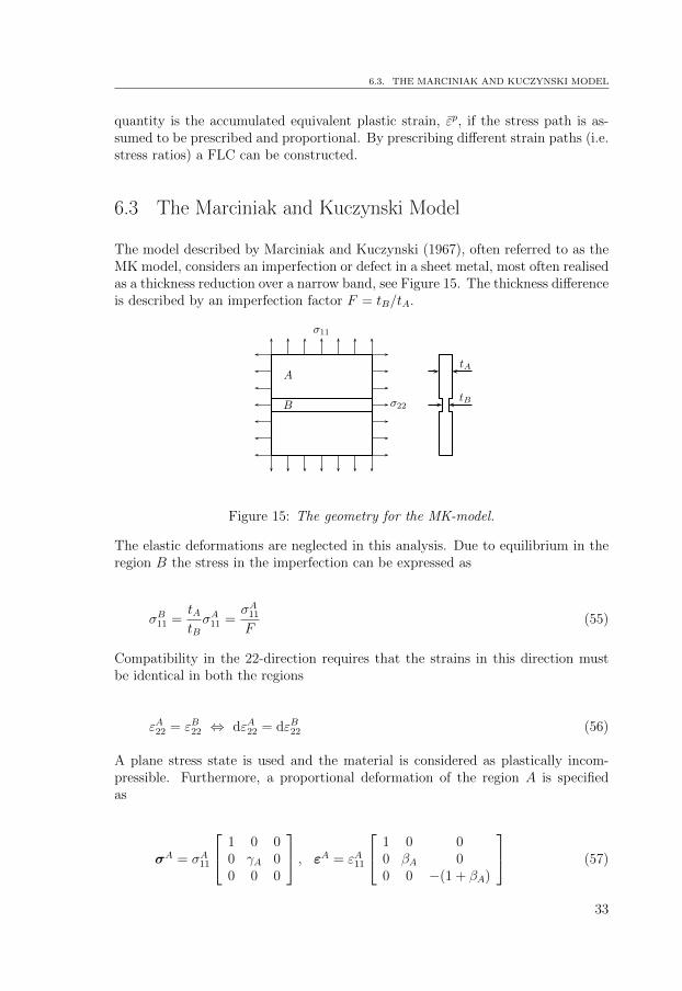
6.3 The Marciniak and Kuczynski Model

The model described by Marciniak and Kuczynski (1967), often referred to as theMK model, considers an imperfection or defect in a sheet metal, most often realisedas a thickness reduction over a narrow band, see Figure 15. The thickness differenceis described by an imperfection factor F = tB/tA.

A

B

σ11

σ22

tA

tB

A0

B0

B1

A1

σ11

σ22

αB

1

αA

1

Figure 15: The geometry for the MK-model.

The elastic deformations are neglected in this analysis. Due to equilibrium in theregion B the stress in the imperfection can be expressed as

σB11 =tAtBσA11 =

σA11

F(55)

Compatibility in the 22-direction requires that the strains in this direction mustbe identical in both the regions

εA22 = εB22 ⇔ dεA22 = dεB22 (56)

A plane stress state is used and the material is considered as plastically incom-pressible. Furthermore, a proportional deformation of the region A is specifiedas

σA = σA11

1 0 00 γA 00 0 0

, εA = εA11

1 0 00 βA 00 0 −(1 + βA)

(57)

33


where γA and βA describe the deformation. The strain ratio, βA, can be expressedas,

βA =∂σ/∂σ22

∂σ/∂σ11

∣∣∣∣σ11=1,σ22=γA,σ12=0

(58)

since that the material is assumed to follow an associated flow rule. The stressσB11 can then be found from Equation 55. Since the stress in the length directionis slightly larger inside the band, the yield surface is first reached here. However,due to the compatibility condition, Equation 56, no plastic deformation can occurbefore the yield surface is also reached for region A. If further deformation occurs,the state of stress in the band is moved on the yield surface towards point B1,see Figure 16(a). At a certain point the yield limit is also reached in the uniformregion, point A1, and plastic deformation can occur. However, due to the restrictionthat the strain in the 22-direction needs to be equal in both regions A and B,the equivalent plastic strain will be different, i.e. εpB > εpA, see Figure 16(b). Acontinuous deformation will increase the difference in equivalent plastic strain andmove the stress state in region B towards the state of plane strain, see Bf in Figure16(a). When the state of plane strain is reached, instability is assumed to occur.

!"

dεA11

dεB11

dεA22 = dεB22

βA

βB

A0

B0

B1

Bf

A1

Af

σ11

σ22

γA

1

&

(a)

dεA11

dεB11

dεA22 = dεB22

βA

βB

(b)

Figure 16: MK model (a) stress state for region A and B and (b) relationshipbetween the strain paths.

34

6.4. FINITE ELEMENT MODEL

6.4 Finite Element Model

Detailed FE models can generally be used to capture the instability phenomena,e.g. Lademo et al. (2004a). To predict the instability, a square patch of elements,see Figure 17, is used with has an inhomogeneity in its thickness distribution.The patch is stretched in different directions to obtain linear strain paths and toproduce the FLC in the forming limit diagram (FLD). The strain paths have beenprescribed such that

δ11 = w0

(eεcosθ − 1

), δ22 = w0

(eεsinθ − 1

)(59)

where w0 is the width of the plate, θ = tanβ is the relationship between the strains,and ε has been given as a smooth function of time.

δ11δ11

δ22

δ22

C

AB

δ11δ11

δ22

δ22

w0

w0

δ11δ11

δ22

δ22

(

Figure 17: Patch of elements for the instability prediction.

The focus of the study is on the relationship between the local thickness strainincrement and the average thickness strain increment, on an area Ω.

ζi =∆ε33,i

∆εΩ33

(60)

The average thickness strain increment is

∆εΩ33 =

1

N

N∑

i=1

∆ε33,i (61)

where N is the number of elements in the domain Ω. Instability is assumed tooccur when ζi reaches a critical value in any element i. However, since the strain-rate shows an oscillating behaviour pattern, it is necessary to define the point of

35


instability over a period of time, viz. ζi needs to exceed a critical value ζc for anumber of time steps nt. Lademo et al. (2004a) describe the thickness variationas a normal distributed random field with mean value µ and standard deviation,usually denoted σ. However, according to Fyllingen et al. (2009) one drawbackwith this method is that the variation depends on the number of nodes. Hence, arefinement of the FE mesh will lead to a different random field. Consequently thevariation in the thickness is described here independently of the FE mesh

t(x, y) = µ(x, y) + Z(x, y) (62)

where both the mean value, µ, and the residual term, Z, may depend on the globalcoordinates x and y. In this work the mean value has been set to a constant value,i.e. µ(x, y) = µ, and for the residual term, Z, a Gaussian zero mean homogeneousrandom field according to Shinozuka and Deodatis (1996) has been used.

6.5 Evaluation of Instability

The different methods presented above can be summarized in an FLD, see Fig-ure 18. As can be seen all models predict about the same instability limit intheir domain of usage. However, all instability models used here, except the FE-based model which can be used for any material model, use a plane stress as-sumption. The material model presented in Chapter 4 is modified to also includea through-thickness normal stress, σND, to obtain a C0 continuous element for-mulation. Therefore, the FE-based model has been used throughout this studyfor instability predictions. A square patch of finite elements is used with an in-homogeneous thickness distribution in order to predict the instability. The patchis stretched such that linear strain paths are obtained in different directions. InLademo et al. (2004a) and Lademo et al. (2004b) the limit strains causing local-isation are considered as the total strains in the patch when an instability hasoccurred. However, in this study the local strains in an element within the locali-sation area are considered. In order to find the strain limit at localised necking inthe patch, two elements are considered: one inside the localisation zone and onesome distance away from it, see Figure 19(a) elements A and B, respectively. Thelimit value is then obtained as the strains in the finite element within the locali-sation zone at a stage when the strains in the distant element do not increase, seeFigure 19(b).

36

−0.1 0 0.1 0.2 0.30

0.1

0.2

0.3

0.4

0.5

Str

ain

in11-

dir

ecti

on,ε 1

1[-]

Strain in 22-direction, ε22 [-]

Swift 1952Hill 1952Hora et al. 1996Marciniak and Kuczynski 1967Lademo et al. 2004

Figure 18: Different models to predict instability.

δ11δ11

δ22

δ22

C

AB

δ11δ11

δ22

δ22

w0

w0

δ11δ11

δ22

δ22

(

(a)

0 0.05 0.1 0.15 0.20

0.1

0.2

0.3

0.4

0.5

0.6

Loca

lst

rain

,ε∗

[-]

Global strain, ε = ln( δ+w0

w0) [-]

A (element inside localisation zone)B (element far away from localisation zone)C (elements across the localisation zone)

(b)

Figure 19: Evaluation procedure for instability limits, (a) chosen elements and(b) local vs. global strain.

Mechanical Experiments7

A number of mechanical tests have been performed to calibrate both the constitu-tive relations and the fracture models. In this study six different mechanical testshave been conducted:

• Pre-deformation

• Tensile

• Shear

• Plane strain

• Bulge

• Nakajima

The pre-deformation specimens have been performed in an MTS hydraulic machinewith a 250 kN load cell. The tensile, shear and plane strain tests have been carriedout in an INSTRON 5582 machine with a 10 kN load cell.

7.1 Pre-Deformation

Pre-deformation of large specimens, according to Figure 20(a), was performed inorder to produce broken strain paths. Due to limitations of the test rig, the speci-men length, width and thickness were 1100 mm, 125 mm and 1.5 mm, respectively.Since all material tests in this work were performed under quasi-static conditionsthe deformation was performed at a constant crosshead speed of 5 mm/min, whichresulted in a strain-rate of approximately 10−4 s−1. The unloading was set to lastfor 1 min. The design of the specimen was made in an attempt to maximize thezone of homogenous strain. The homogeneity at the centre of the specimen wasconfirmed both by FE simulation, see Figure 20(b), and by ocular measurements.The mid section of the specimen was divided into 16 equal sections, in which thethickness, width and length were measured both before and after completed load-ing. The pre-deformations were performed both in the RD and in the TD, i.e.ψ = 0 and ψ = 90 according to Figure 21. For each direction the materials havebeen pre-deformed to two significant strain levels; one level chosen close to thestrain causing diffused necking and the other level chosen to approximately half of

39

CHAPTER 7. MECHANICAL EXPERIMENTS

the first one. The levels of pre-straining for each material and direction are dis-played in Table 4. After the pre-straining operation tensile, shear and plane strainspecimens have been machined out from the centre part of the larger specimens,see Figure 20(c).

(a)

(b)

(c)

Figure 20: a) Geometry of pre-strain specimen. b) Sketch including some cut outspecimens. c) Distribution of longitudinal plastic strain. The iso-curves representstrain levels ranging from 9% to 11 % with 0.2% steps. Dimensions are given inmm.

ψ

φ

θ

RD

Figure 21: Angles defining pre-strain directions, ψ, and directions of subsequenttestings, φ = ψ + θ.

40

7.2. TENSILE TEST

Table 4: Approximative plastic strains after pre-straining.

Material Docol 600DP Docol 1200M

Direction RD TD RD TD

εp [%] 5 10 4.5 8 0.5 1 0.4 0.7

7.2 Tensile Test

The tensile tests have been used to represent the hardening up to diffuse neckingand also to represent the anisotropy of the yield function and the kinematic hard-ening. Tensile test specimens according to Figure 22 have been performed in theφ = 0, 45 and 90 directions, where φ is the angle to the RD, see Figure 21, bothfor the as-received and the pre-deformed material specimens. During the tensiletests the load, elongation and width contraction were recorded. The elongation, εL,has been measured by an INSTRON 2620-601 extensometer with a gauge lengthof L0 = 12.5 mm, and the width contraction, εW , has been measured with anMTS 632.19B-20 extensometer over the entire width of the specimen. The defor-mation was performed with a constant crosshead speed of 0.45 mm/min, whichresulted in a strain-rate of approximately 10−4 s−1. The anisotropy in yield stressand plastic flow were evaluated directly from the tensile tests of the as-receivedspecimens. Also the hardening behaviour up to diffused necking is obtained di-rectly from the experimental data. Numerical simulations and inverse modellingare used to identifying the kinematic hardening of the pre-strained materials.

Figure 22: Geometry of the tensile test with dimensions in mm.

7.3 Simple Shear Test

The geometry of the simple shear test specimen used in this study is shown inFigure 23. The shear tests are performed on both as-received and on pre-deformedspecimens in the φ = 0, 45 and 90 directions. The two attachments for theshear test have been in the form of a pin at both ends to prevent the specimensfrom rotational loading. In order to obtain a strain-rate of approximately 10−4 s−1,the displacement rate of 0.03 mm/min has been used. The shear test results areused in combination with inverse modelling to gain an accurate description of the

41


hardening behaviour for large strains, to find the yieldsurface exponent, and tocalibrate the Cockroft-Latham fracture model.

Figure 23: Geometry of the shear specimen with dimensions in mm.

7.4 Plane Strain Test

The geometry of the plane strain test (notched tensile test) is shown in Figure 24.Similar designs have been utilised in other studies, e.g. Lademo et al. (2008).The plane strain tests were performed in φ = 0, 45 and 90 directions, with adisplacement rate of 0.06 mm/min. During the test the load, grip motion, widthreduction and midsection elongation were measured. The latter was measured byan INSTRON 2620-601 extensometer width a gauge length of 23 mm, while thewidth reduction was measured by an MTS 632.19B-20 extensometer. The planestrain test is used in combination with inverse modelling in order to calibrate theBressan-William fracture model.

7.5 Balanced Biaxial Test

A balanced biaxial bulge test was performed on the virgin materials. The pressurewas applied with a punch made of silicon and a pattern of randomly placed dotswas sprayed on the sheet surface. The specimen was video recorded by two camerasduring the subsequent testing. The in-plane strains and the radius of the bulgewere then evaluated from the recording of the pattern motion using an ARAMISstrain measurement system. Balanced biaxial tests have been used in order toobtain the stress and strain ratios rb and kb, respectively, cf. Sigvant et al. (2009).

42

7.6. NAKAJIMA TEST

Figure 24: Geometry of the plane strain specimen with dimensions in mm.

7.6 Nakajima Test

A number of Nakajima tests, see ISO (2008), have been conducted in order toevaluate the failure behaviour. The tests were made on virgin material and thegeometries, see Figure 25, were chosen so that the first quadrant (ε1 ≥ 0, ε2 ≥ 0)of the FLD was covered.

(a) (b)

Figure 25: Nakajima specimen geometry dimmensions in mm: (a) circular (b)with different waists (L=130,140,150,160,165 and 170 mm).

The Nakajima tests were performed in an Interlaken ServoPress 150. The machinehas a punch diameter of 100 mm and a load cell of 550 kN. The clamping forcewas limited to 700 kN and the punch motion was set to 1 mm/s. During thetest the force and displacement of the punch was recorded. The specimens were

43


treated with three layers of oil and plastic film to reduce friction. Before thetest a mesh with a 2 mm grid size was etched onto the specimens. The strainswere then evaluated optically by an AutoGrid 4.1 Strain Analysis System, whichused information from four cameras, each of which recorded 30 images per secondduring the test. The image just before the fracture was used to evaluate the limitstrains. Since the image just before fracture is used, the strains may be well pastthe limit of localised necking. Therefore a method similar to the one described byBragard et al. (1972) has been used to evaluate the limit strains at the onset oflocalised necking. This method is straightforward and the major and minor straindistributions on a few lines across the instability are considered. Afterwards thestrains inside the localised region are excluded and a polynomial fit is adopted tothe remaining strains. The maximum strain from this polynomial is chosen as themajor strain limit, see Figure 26. For the minor strain a linear fit is performed atthe location of the maximum.

−15 −10 −5 0 5 10 15−0.1

0

0.1

0.2

0.3

0.4

Str

ain,ε

[-]

Position along, x [mm]

Major strainMinor strainPolynomial Fit

Excluded Points

Minor Strain atLocalised Necking

Major Strain atLocalised Necking

(a)

- -

x

$ %

%

(b)

Figure 26: Illustration of the Bragard et al. (1972) method; (a) polynomial fitto strains and (b) lines of elements across the localisation zone used for strainevaluation.

44

Finite Element Modelling8

Finite element analyses of the tensile, shear, plane strain and Nakajima experimentshave been performed using LS-DYNA, see Hallquist (2009). All FE meshes havebeen produced in TrueGrid, see Rainsberger (2006). A non-local treatment of thefracture parameters is needed in order to reduce the mesh dependency. However,the C0 continuity of the thickness across the element edges as obtained by theuse of an extended shell element formulation contributes to a regularisation ofthe thickness strain, and thus reduces the mesh dependency. The introduction ofthe normal through-thickness stress, σND, enables a C0 continuity in the elementformulation, cf. Borrvall and Nilsson (2003). However, the inclusion of the normalstress also introduces transversal shear stresses and strains, see Figure 27. Thetransversal shear stresses are not entering into the elasto-plastic constitutive model,but are updated elastically.

3 !

5

<

εxz = 0

5

<

εxz = 0

&

⎧⎪⎪⎪⎪⎪⎪⎪⎪⎪⎪⎪⎪⎨⎪⎪⎪⎪⎪⎪⎪⎪⎪⎪⎪⎪⎩

σxx

σyy

σzz

σxy

σyz

σzx

⎫⎪⎪⎪⎪⎪⎪⎪⎪⎪⎪⎪⎪⎬⎪⎪⎪⎪⎪⎪⎪⎪⎪⎪⎪⎪⎭

=

⎡⎢⎢⎢⎢⎢⎢⎢⎢⎢⎢⎢⎢⎣

λ+ 2μ λ λ 0 0 0

λ λ+ 2μ λ 0 0 0

λ λ λ+ 2μ 0 0 0

0 0 0 μ 0 0

0 0 0 0 κμ 0

0 0 0 0 0 κμ

⎤⎥⎥⎥⎥⎥⎥⎥⎥⎥⎥⎥⎥⎦

⎧⎪⎪⎪⎪⎪⎪⎪⎪⎪⎪⎪⎪⎨⎪⎪⎪⎪⎪⎪⎪⎪⎪⎪⎪⎪⎩

εxx

εyy

εzz

εxy

εyz

εzx

⎫⎪⎪⎪⎪⎪⎪⎪⎪⎪⎪⎪⎪⎬⎪⎪⎪⎪⎪⎪⎪⎪⎪⎪⎪⎪⎭

%1

μ = E2(1+ν) λ = Eν

(1+ν)(1−2ν)%2

&

(a)

3 !

5

<

εxz = 0

5

<

εxz = 0

&

⎧⎪⎪⎪⎪⎪⎪⎪⎪⎪⎪⎪⎪⎨⎪⎪⎪⎪⎪⎪⎪⎪⎪⎪⎪⎪⎩

σxx

σyy

σzz

σxy

σyz

σzx

⎫⎪⎪⎪⎪⎪⎪⎪⎪⎪⎪⎪⎪⎬⎪⎪⎪⎪⎪⎪⎪⎪⎪⎪⎪⎪⎭

=

⎡⎢⎢⎢⎢⎢⎢⎢⎢⎢⎢⎢⎢⎣

λ+ 2μ λ λ 0 0 0

λ λ+ 2μ λ 0 0 0

λ λ λ+ 2μ 0 0 0

0 0 0 μ 0 0

0 0 0 0 κμ 0

0 0 0 0 0 κμ

⎤⎥⎥⎥⎥⎥⎥⎥⎥⎥⎥⎥⎥⎦

⎧⎪⎪⎪⎪⎪⎪⎪⎪⎪⎪⎪⎪⎨⎪⎪⎪⎪⎪⎪⎪⎪⎪⎪⎪⎪⎩

εxx

εyy

εzz

εxy

εyz

εzx

⎫⎪⎪⎪⎪⎪⎪⎪⎪⎪⎪⎪⎪⎬⎪⎪⎪⎪⎪⎪⎪⎪⎪⎪⎪⎪⎭

%1

μ = E2(1+ν) λ = Eν

(1+ν)(1−2ν)%2

&

(b)

Figure 27: Element formulation (a) ordinary plane stress element (b) a continuousthickness based element.

The transversal shear stresses will prevent the localisation and will thus contributeto a stiffening effect. An improved result can be obtained by using an effectivestress, which takes all stresses into account or by reducing the transversal shearstresses by a correction factor according to the theory of Reissner-Mindlin, seeHughes (2000). The latter method has been adopted here, i.e. the transversalshear stresses have been reduce by a shear correction factor, κ, according to

σyz = κE

2(1 + ν)εyz, σzx = κ

E

2(1 + ν)εzx (63)

45

CHAPTER 8. FINITE ELEMENT MODELLING

where E and ν are the Young’s modulus and Poisson’s ratio, respectively. However,κ will also affect the hardening after diffused necking. Thus, the hardening afterdiffused necking has been modified compared to what was presented in Larssonet al. (2011) in order to maintain a good agreement between simulations and testresults. The parameters of the hardening after necking and the shear correctionfactor, κ, have been obtained from inverse modelling of the tensile, shear and planestrain tests.

8.1 Pre-Straining

FE analyses of the tensile and shear experiments have been performed both forvirgin and pre-strained specimens. The pre-straining operation, which producedthe non-proportional strain paths, was made by stretching one single element tothe strain levels shown in Table 4. The back-stress tensor, α, equivalent plasticstrain, εp, and fracture parameter, W , are subsequently mapped on the modelsof the small specimens used in the subsequent analyses, see Figure 28. Since thestrain field from stretching one single element is mapped on to all elements of themodel of each small specimen, no strain inhomogeneities will be present in thesubsequent simulations.

" #$

3

'#"

F F

x

y

(

-

ψ

7 "

α, εp,W⇒ F F

x

y

(

-

φ

&

Figure 28: One pre-strained element from which the backstress, α, equivalent plasticstrain, εp, and fracture parameter, W , are mapped to the models for the subsequentanalyses.

8.2 Tensile Test

The FE model of the tensile specimen is shown in Figure 29. It consists of about5500 shell elements. The characteristic element size is approximately 0.5 mm. Agood agreement between the stress-strain relationship simulation and tensile testresults can be observed up to diffused necking, as reported in Larsson et al. (2011).By introducing a shear correction factor κ = 0.05 in the shell formulation and mod-ifying the hardening curve after diffuse necking, improved agreement was obtainedbetween the simulation and test results, even for the crosshead displacement afterdiffuse necking, see Figure 30.

46

8.3. SHEAR TEST

Figure 29: FE model of the tensile test specimen.

0 5 10 150

5

10

15

Forc

e,F

[kN

]

Displacement, δ [mm]

φ = 0 exp.φ = 0 sim.φ = 45 exp.φ = 45 sim.φ = 90 exp.φ = 90 sim.

(a)

0 1 2 3 40

5

10

15

20

25

30

Forc

e,F

[kN

]



(b)

Figure 30: Results from tensile test of virgin material in different material direc-tion (a) Docol 600DP (b) Docol 1200M.

8.3 Shear Test

The FE model of the shear specimen is shown in Figure 31. It consists of about12500 shell elements. The characteristic element size in the shear zone is approxi-mately 0.06 mm, see Figure 31(b). A good agreement between simulation resultsand the force-displacement relationships of the shear experiment was found afterthe correction of the shear factor and modification of the hardening curve, seeFigure 32.

(a) (b)

Figure 31: (a) FE model of the shear specimen. (b) Details of the mesh in theshear zone.

47


0 0.5 1 1.5 20

0.5

1

1.5

2

2.5

3

For

ce,F

[kN

]



(a)

0 0.5 1 1.50

0.5

1

1.5

2

2.5

3

3.5

4

For

ce,F

[kN

]



(b)

Figure 32: Results from shear test of virgin material in different material direction(a) Docol 600DP (b) Docol 1200M.

8.4 Plane Strain Test

The FE model of the plane strain test specimen can be seen in Figure 33. Themodel consists of about 7900 shell elements. The element size in the centre ofthe specimen is approximately 0.2 mm. The C0 continuous element formulationused through this work enabled an improved correspondence between FE simu-lation and experimental results compared to the conventional shell element for-mulation, see Figure 34. A good agreement between simulation results and theforce-displacement relations for the plane strain tests was found, see Figure 35.

Figure 33: FE model of the plane strain specimen.

48

8.4. PLANE STRAIN TEST

0 0.5 1 1.5 2 2.5 30

5

10

15

20

25For

ce,F

[kN

]


ExperimentPlane StressWith Normal Stress

Figure 34: Different element formulation used for simulations of the plane straintest.

0 0.5 1 1.5 2 2.5 30

5

10

15

20

25

For

ce,F

[kN

]



(a)

0 0.5 1 1.50

10

20

30

40

50

For

ce,F

[kN

]



(b)

Figure 35: Results from plane strain test of virgin material in different materialdirection (a) Docol 600DP (b) Docol 1200M.

49


8.5 Nakajima Test

The characteristic element size in the FE models of the Nakajima specimens wasapproximately 0.75 mm. Since the Nakajima tests are used for prediction of thefailure behaviour, it was necessary to introduce a small disturbance of the thicknessin order to capture the instability correctly. The thickness variation has here beengiven using the same method as for the patch discussed in Chapter 6. The Nakajimatests were used in order to evaluate the failure behaviour and a good agreementwas obtained. However it has been seen that, the friction chosen between thespecimen and punch surface in the simulation model is of a great importance inthe prediction of the instability. The friction used in all simulation models hastherefore been chosen such that the instability is predicted as close as possible tothe specimen with a waist of 60 mm, see Figure 36.

0 5 10 15 20 25 300

10

20

30

40

50

60

70

80

Punch

forc

e,F

[kN

]

Punch displacement, δ [mm]

ExperimentsSim. µ=0.01Sim. µ=0.05Sim. µ=0.10

0

500

1000

1500

2000

Fra

cture

par

amet

er,W

[MPa]

F

W

Figure 36: Different friction for prediction of instability of the Nakajima test ofDocol 600DP in RD with a waist of 60 mm.

50

Conclusions and Discussion9

One major objective of the proposed fracture models was that they should beeasy to calibrate. Since both the models investigated in this thesis have only onematerial parameter, just one basic mechanical experiment and the correspondingFE simulation are sufficient for calibration. However, in several loading situations,it is hard to identify whether the fracture is initiated prior to the instability orafter. In the plane strain test a localisation is observed before fracture, both inthe FE simulations and the experiments. The fracture parameters calibrated fromthese experiments will then depend on how well the deformation is captured inthe localised zone. It may be argued that the plane strain test should not be usedfor this calibration, since the instability arises before the fracture. The fracturemodel calibrated from the plane strain test can, since the instability arises beforethe fracture, be considered as an upper limit for the fracture within the FLD.

Even if one single experiment and one FE simulation are sufficient to calibrateeach of the fracture models used in this study, one fracture parameter value wasevaluated from specimens in all material directions of the virgin material. Fromthe evaluation of these results it can be seen that there is a large variation inthe parameters obtained from the different material directions and also within thedifferent tests in the same direction. The behaviour of the material in differentmaterial directions cannot be predicted by the fracture models chosen for thisstudy, since the fracture models adopted are isotropic, although the constitutivemodel is anisotropic. In order to predict the different fracture behaviour observedin different directions, an anisotropic fracture model is needed. The variation ofthe fracture appearance within the same material direction can be explained by thefact that the fracture is strongly influenced by inclusions and impurities within thematerial, and since these are located differently in different specimens the fractureswill differ. It may thus be preferable to specify the fracture parameters with lowerand upper limits rather than as a specific value.

Most of the Nakajima experiments and simulations show an instability before frac-ture. Consequently the prediction of this instability is very important. However,in this study the prediction of the instability is made by using the constitutivemodel and FE models with significantly dense meshes. In order to obtain a goodprediction it is therefore necessary to carefully calibrate the material and fracturemodels before subsequent use. Since the shape of the yield surface, the harden-ing law and also the element formulation all affect the instability. Therefore it

51

CHAPTER 9. CONCLUSIONS AND DISCUSSION

is important to choose suitable mechanical experiments and element formulationfor the calibration. The validation of the failure behaviour has been performedin experiments and FE simulations of the Nakajima tests. In the evaluation ofthe quality of the fracture and instability predictions, their representation is veryimportant. One direct method is to compare the force-displacement curves fromsimulations and experiments directly. However, since the FLD is a commonly-usedtool for failure prediction, it is also useful to represent failure predictions as FLCin an FLD. The curves representing the locus of different failures, i.e. ductile frac-ture, shear fracture and instability, are easy to interpret. Their representation ofthe strains from the experiments causing localisation is, however, not that trivial.There are many approaches on how to evaluate the forming limit. In experimentsin this study, the deformation was monitored during the deformation, and thus thestrains were captured close to the instance of fracture. However, the strains maythen be well past the onset of localisation and the limit of instability needs to beevaluated using a different method. In some methods a few grid points outside thefracture zone are evaluated and the strains there are considered to be the limit.In this study the strains of failure are evaluated with a polynomial fit across theinstability zone.

The results obtained from the failure prediction are generally in a good agreementwith experiments. However, a large variation of fracture parameters is observedand an interval in its values is to be preferred, since some variation is alwaysobtained in mechanical experiments. The variation in the mechanical experimentsmay be caused by a number of different factors such as variation in setup, variationin material and measurement error.

52

Review of Appended Papers10

Paper I

A study of high strength steels undergoing non-linear strain paths -Experiments and modelling

This paper presents an evaluation of the constitutive behaviour, including plasticanisotropy and mixed isotropic-kinematic hardening of two high strength steels,Docol 600DP and Docol 1200M, during strain path changes. A series of tensileand shear tests was performed on both virgin and pre-strained materials. The ini-tial anisotropy and work hardening parameters were obtained from tensile tests,shear tests and a bulge test of the virgin material, whereas the kinematic harden-ing parameters were identified by comparing numerical predictions to experimentalresults related to the pre-strained materials. Numerical predictions using the ob-tained parameters agree well with the experimental results, both in the case ofproportional, and under non-proportional strain paths.

Paper II

Failure of high strength steel sheet - Experiments and modelling

Failure in thin sheet metal structures of ductile material is usually caused by oneof, or a combination of, the following: ductile fracture, shear fracture or localisedinstability. In this paper the failure of the high strength steel Docol 600DP and theultra high strength steel Docol 1200M is explored. The constitutive model usedin this study includes plastic anisotropy and mixed isotropic-kinematic hardening.For modelling of the ductile and shear fracture the models presented by Cockroft-Latham and Bressan-Williams have been used. The instability phenomenon isdescribed by the constitutive law and the finite element (FE) models. For calibra-tion of the failure models and validation of the results, an extensive experimentalseries has been conducted including shear tests, plane strain tests and Nakajimatests. The geometries of the Nakajima tests have been chosen so that the first

53

CHAPTER 10. REVIEW OF APPENDED PAPERS

quadrant of the forming limit diagram (FLD) were covered. The results are pre-sented both in an FLD and using prediction of force-displacement response of theNakajima test employing element erosion during the FE simulations. The classicalapproach for failure prediction is to compare the FE simulations with experimentaldetermined forming limit curves (FLC). Here phenomenological models have beenused which show promising results. The benefit of using phenomenological modelsis the ability to follow failure behaviour for more complex loading paths.

54

Bibliography

Aretz, H., 2004. Numerical restrictions of the modified maximum force crite-rion for prediction of forming limits in sheet metal forming. Modelling andSimulation in Materials Science and Engineering 12 (4), 677–692.

Aretz, H., 2005. A non-quadratic plane stress yield function for orthotropic sheetmetals. Journal of Materials Processing Technology 168 (1), 1 – 9.

Askeland, D. R., 1998. The Science and Engineering of Materials. Nelson ThornesLtd, Sheffield.

Bai, Y., Wierzbicki, T., 2008. A new model of metal plasticity and fracture withpressure and Lode dependence. International Journal of Plasticity 24 (6),1071 – 1096.

Banabic, D., Barlat, F., Cazacu, O., Kuwabara, T., 2010. Advances in anisotropyand formability. International Journal of Material Forming 3, 165–189.

Bao, Y., Wierzbicki, T., 2004. On fracture locus in the equivalent strain andstress triaxiality space. International Journal of Mechanical Sciences 46 (1),81 – 98.

Belytschko, T., Liu, W. K., Moran, B., 2000. Nonlinear Finite Elements forContinua and Structures. Wiley, Chichester.

Borrvall, T., Nilsson, L., 2003. Revision of the implementation of material 36 inLS-DYNA. Engineering Reaserch Nordic AB, Linkoping, private communi-cation.

Bragard, A., Baret, J.-C., Bonnarnes, H., 1972. A simplified technique to deter-mine the FLD at the onset of necking. Report no. 33, Rapport Centre deRecherche de la Metallurgie, Liege.

Bressan, J., Williams, J., 1983. The use of a shear instability criterion to predictlocal necking in sheet metal deformation. International Journal of MechanicalSciences 25 (3), 155–168.

Cockroft, M. G., Latham, D. J., 1968. Ductility and the workability of metals.Journal of the Institute of Metals 96, 33–39.

Dieter, G. E., 1986. Mechanical Metallurgy. McGraw-Hill, New York.

55


Frederick, C., Armstrong, P., 2007. A mathematical representation of the multi-axial Bauschinger effect. Materials at High Temperatures 24 (1), 1–26.

Fyllingen, O., Hopperstad, O., Lademo, O.-G., Langseth, M., 2009. Estimationof forming limit diagrams by the use of the finite element method and MonteCarlo simulation. Computers and Structures 87 (1-2), 128 – 139.

Gurson, A., 1977. Continuum theory of ductile rupture by void nucleation andgrowth: Part I - yield criteria and flow rules for porous ductile media. Journalof Engineering Materials and Technology 99 (1), 2 – 15.

Hallquist, J., 2009. LS-DYNA Theory Manual. Livermore Software TechnologyCorporation, Livermore.

Han, H. N., Kim, K.-H., 2003. A ductile fracture criterion in sheet metal formingprocess. Journal of Materials Processing Technology 142 (1), 231 – 238.

Hill, R., 1952. On discontinuous plastic states, with special reference to localizednecking in thin sheets. Journal of the Mechanics and Physics of Solids 1 (1),19 – 30.

Hollomon, J. H., 1945. Tensile deformation. Transaction of the American Insti-tute of Mining, Metallurgical and Petroleum Engineers 162, 268–290.

Hooputra, H., Gese, H., Dell, H., Werner, H., 2004. A comprehensive failuremodel for crashworthiness simulation of aluminium extrusions. InternationalJournal of Crashworthiness 9 (5), 449 – 63.

Hora, P., Tong, L., Reissner, J., 1996. A prediction method for ductile sheet metalfailure in FE-simulation. Proceedings of the 3’rd International ConferenceNumisheet’96, Dearborn, Michigan, 252–256.

Hosford, W., Cadell, R., 1993. Metal Forming Mechanics and Metallurgy. Prentis-Hall, New York.

Hughes, T. J. R., 2000. The Finite Element Method - Linear Static and DynamicFinite Element Analysis. Dover Publications, Mineola, New York.

ISO, 2008. Metallic materials -sheet and strip - determination of forming limitcurves - Part 2: Determination of forming limit curves in the laboratory.12004-2:2008, Austrian Standards Institute, Wien.

Johnson, G. R., Cook, W. H., 1983. Fracture characteristics of three metals sub-jected to various strains, strain rates, temperatures and pressures. SeventhInternational Symposium on Ballistics, Hague, 1–7.

Johnson, G. R., Cook, W. H., 1985. Fracture characteristics of three metalssubjected to various strains, strain rates, temperatures and pressures. Engi-neering Fracture Mechanics 21 (1), 31 – 48.

Krauss, G., 2005. Steels Processing, Structure, and Preformance. ASM Interna-tional Materials Park, Ohio.

56

Lademo, O.-G., Berstad, T., Hopperstad, O. S., Pedersen, K. O., 2004a. A nu-merical tool for formability analysis of aluminium alloys. Part I: Theory.Steel Grips 2, 427–432.

Lademo, O.-G., Pedersen, K., Berstad, T., Furu, T., Hopperstad, O., 2008. Anexperimental and numerical study on the formability of textured AlZnMgalloys. European Journal of Mechanics - A/Solids 27 (2), 116 – 140.

Lademo, O.-G., Pedersen, K. O., Berstad, T., Hopperstad, O. S., 2004b. A numer-ical tool for formability analysis of aluminium alloys. Part II: Experimentalvalidation. Steel Grips 2, 433–437.

Larsson, R., Bjorklund, O., Nilsson, L., Simonsson, K., 2011. A study of highstrength steels undergoing non-linear strain paths - experiments and mod-elling. Journal of Materials Processing Technology 211, 122–132.

Lemaitre, J., 1985. A continuous damage mechanics model for ductile fracture.Journal of Engineering Materials and Technology 107, 83–89.

Lemaitre, J., Chaboche, J.-L., 1990. Mechanics of Solid Materials. CambridgeUniversity Press, Cambridge.

Marciniak, Z., Kuczynski, K., 1967. Limit strains in the processes of stretch-forming sheet metal. International Journal of Mechanical Sciences 9 (9),609–620.

Olsson, K., Gladh, M., Hedin, J.-E., Larsson, J., 2006. Microalloyed high-strengthsteels. Advanced Materials and Processes 164 (8), 44–46.

Opbroek, E. G., 2009. Advanced high strength steel application guidelines. Tech.Rep. WorldAutoSteel.

Oyane, M., Sato, T., Okimoto, K., Shima, S., 1980. Criteria for ductile fractureand their applications. Journal of Mechanical Working Technology 4 (1), 65– 81.

Rainsberger, R., 2006. TrueGrid User’s Manual. XYZ Scientific Applications,Inc., Livermore.

Shinozuka, M., Deodatis, G., 1996. Simulation of multi-dimensional Gaussianstochastic fields by spectral representation. Applied Mechanics Reviews 49,29–53.

Sigvant, M., Mattiasson, K., Vegter, H., Thilderkvist, P., 2009. A viscous pressurebulge test for the determination of a plastic hardening curve and equibiaxialmaterial data. International Journal of Material Forming 2 (4), 235–242.

Swift, H. W., 1952. Plastic instability under plane strain. Journal of the Mechan-ics and Physics of Solids, 1, 1–18.

Teirlinck, D., Zok, F., Embury, J., Ashby, M., 1988. Fracture mechanism mapsin stress space. Acta Metallurgica 36 (5), 1213 – 1228.

57


Voce, E., 1948. The relationship between stress and strain for homogenus defor-mation. Journal of the Institute of Metals 74, 537–562.

Wierzbicki, T., Bao, Y., Lee, Y.-W., Bai, Y., 2005. Calibration and evaluation ofseven fracture models. International Journal of Mechanical Sciences 47 (4-5),719 – 743.

Wilkins, M. L., Streit, R. D., Reaugh, J. E., 1980. Cumulative-strain-damagemodel of ductile fracture: Simulation and prediction of engenering fracturetests. Tech. Rep. Lawrence Livermore National Laboratory, Livermore.

58

modelling of failure in high strength steel sheets

Documents