Modelling Internal Solitary Wavesand the Alternative Ostrovsky

Equation

by

Yangxin He

A thesispresented to the University of Waterloo

in fulfillment of thethesis requirement for the degree of

Master of Mathematicsin

Applied Mathematics

Waterloo, Ontario, Canada, 2014

c© Yangxin He 2014

I hereby declare that I am the sole author of this thesis. This is a true copy of the thesis,including any required final revisions, as accepted by my examiners.

I understand that my thesis may be made electronically available to the public.

ii

Abstract

Internal solitary waves (ISWs) are commonly observed in the ocean, and they play im-portant roles in many ways, such as transport of mass and various nutrients throughpropagation. The fluids considered in this thesis are assumed to be incompressible, invis-cid, non-diffusive and to be weakly affected by the Earth’s rotation. Comparisons of theevolution of an initial solitary wave predicted by a fully nonlinear model, IGW, and twoweakly-nonlinear wave equations, the Ostrovsky equation and a new alternative Ostrovskyequation, are done.

Resolution tests have been run for each of the models to confirm that the current choicesof the spatial and time steps are appropriate. Then we have run three numerical simula-tions with varying initial wave amplitudes. The rigid-lid approximation has been used forall of the models. Stratification, flat bottom and water depth stay the same for all threesimulations.

In the simulation analysis, we use the results from the IGW as the standard. Both ofthe two weakly nonlinear models give fairly good predictions regarding the leading waveamplitudes, shapes of the wave train and the propagation speeds. However, the weaklynonlinear models over-predict the propagation speed of the leading solitary wave and thatthe alternative Ostrovsky equation gives the worst prediction. The difference between thetwo weakly nonlinear models decreases as the initial wave amplitude decreases.

iii

Acknowledgements

I would like to take this opportunity to thank my supervisor, Professor Kevin Lamb, forhis patient guidance and support. This thesis would not have been completed without him.

I would also like to thank Professors Marek Stastna and Francis Poulin for being mydefense committee and reading my thesis, especially in providing constructive feedbackand correcting my awkward sentences.

Many thanks to Anson for standing by me and making my life special.

iv

Dedication

To my mom.

v

Contents

List of Tables ix

List of Figures xiii

1 Introduction 1

1.1 Observations and Importance of Internal Waves . . . . . . . . . . . . . . . 1

1.2 Wave Models . . . . . . . . . . . . . . . . . . . . . . . . . . . . . . . . . . 2

1.2.1 Weakly Nonlinear Models . . . . . . . . . . . . . . . . . . . . . . . 2

1.2.2 Fully Nonlinear Models . . . . . . . . . . . . . . . . . . . . . . . . . 4

1.3 Thesis Structure and Goals . . . . . . . . . . . . . . . . . . . . . . . . . . . 5

2 Theoretical Background 6

2.1 Fully Nonlinear Equations with Rotation . . . . . . . . . . . . . . . . . . . 6

2.1.1 f-plane Approximation . . . . . . . . . . . . . . . . . . . . . . . . . 6

2.1.2 Boussinesq Approximation . . . . . . . . . . . . . . . . . . . . . . . 7

2.2 Linearized Equations . . . . . . . . . . . . . . . . . . . . . . . . . . . . . . 9

2.2.1 Buoyancy Frequency . . . . . . . . . . . . . . . . . . . . . . . . . . 10

2.2.2 Constant N . . . . . . . . . . . . . . . . . . . . . . . . . . . . . . . 10

2.2.3 Non-constant N . . . . . . . . . . . . . . . . . . . . . . . . . . . . . 12

2.3 Dubreil-Jacotin-Long (DJL) Equation . . . . . . . . . . . . . . . . . . . . . 14

vi

3 Weakly Nonlinear Equations 17

3.1 Derivation of the Ostrovsky Equation . . . . . . . . . . . . . . . . . . . . . 17

3.1.1 Boundary Conditions . . . . . . . . . . . . . . . . . . . . . . . . . . 18

3.1.2 Non-dimensionalization . . . . . . . . . . . . . . . . . . . . . . . . . 18

3.1.3 Asymptotic Expansion . . . . . . . . . . . . . . . . . . . . . . . . . 20

3.1.4 Properties of Alternative Ostrovsky equation . . . . . . . . . . . . . 24

3.1.5 Ostrovsky Equation . . . . . . . . . . . . . . . . . . . . . . . . . . . 25

3.2 KdV-type Equations . . . . . . . . . . . . . . . . . . . . . . . . . . . . . . 27

3.2.1 Two-layer Fluid . . . . . . . . . . . . . . . . . . . . . . . . . . . . . 28

3.2.2 Solitary Wave Solutions . . . . . . . . . . . . . . . . . . . . . . . . 28

3.3 Solution Analysis to KdV-type Equations . . . . . . . . . . . . . . . . . . . 31

3.3.1 Linearized KdV Equation . . . . . . . . . . . . . . . . . . . . . . . 32

3.3.2 Linearized Ostrovsky Equation . . . . . . . . . . . . . . . . . . . . 34

3.3.3 Linearized Alternative form of Ostrovsky Equation . . . . . . . . . 36

3.3.4 Comparisons . . . . . . . . . . . . . . . . . . . . . . . . . . . . . . 39

4 Numerical Model Setup 43

4.1 Fully Nonlinear Model: IGW . . . . . . . . . . . . . . . . . . . . . . . . . . 43

4.1.1 Solitary Wave Initialization . . . . . . . . . . . . . . . . . . . . . . 43

4.1.2 Stratification, Topography and Boundary Conditions . . . . . . . . 44

4.1.3 Numerical Method . . . . . . . . . . . . . . . . . . . . . . . . . . . 45

4.2 Weakly Nonlinear Model . . . . . . . . . . . . . . . . . . . . . . . . . . . . 46

4.2.1 Alternative Ostrovsky equation solver . . . . . . . . . . . . . . . . . 46

4.2.2 Ostrovsky equation solver . . . . . . . . . . . . . . . . . . . . . . . 52

5 Simulation Results 54

5.1 Resolution Test . . . . . . . . . . . . . . . . . . . . . . . . . . . . . . . . . 54

5.1.1 IGW model . . . . . . . . . . . . . . . . . . . . . . . . . . . . . . . 54

5.1.2 Ostrovsky Solver . . . . . . . . . . . . . . . . . . . . . . . . . . . . 55

5.1.3 Alternative Ostrovsky Solver . . . . . . . . . . . . . . . . . . . . . . 57

vii

5.2 Comparisons of IGW, Ostrovsky and alternative Ostrovsky equations . . . 58

5.2.1 Amplitude = 79 m . . . . . . . . . . . . . . . . . . . . . . . . . . . 58

5.2.2 Amplitude = 43 m . . . . . . . . . . . . . . . . . . . . . . . . . . . 62

5.2.3 Amplitude = 23 m . . . . . . . . . . . . . . . . . . . . . . . . . . . 65

5.3 Simulation Analysis . . . . . . . . . . . . . . . . . . . . . . . . . . . . . . . 69

6 Conclusion 78

6.1 Summary . . . . . . . . . . . . . . . . . . . . . . . . . . . . . . . . . . . . 78

6.2 Future Work . . . . . . . . . . . . . . . . . . . . . . . . . . . . . . . . . . . 79

References 85

viii

List of Tables

5.1 The amplitude decay of the leading wave . . . . . . . . . . . . . . . . . . . 61

5.2 The amplitude decay of the leading wave . . . . . . . . . . . . . . . . . . . 65

5.3 The amplitude decay of the leading wave . . . . . . . . . . . . . . . . . . . 69

5.4 amplitude = 79m . . . . . . . . . . . . . . . . . . . . . . . . . . . . . . . . 72

5.5 amplitude = 43m . . . . . . . . . . . . . . . . . . . . . . . . . . . . . . . . 72

5.6 amplitude = 23m . . . . . . . . . . . . . . . . . . . . . . . . . . . . . . . . 72

5.7 Wavenumber k for different models at t = 3e5 s. . . . . . . . . . . . . . . . 77

ix

List of Figures

2.1 Frequency vs wavenumber for the linearized equations with rotation. . . . . 11

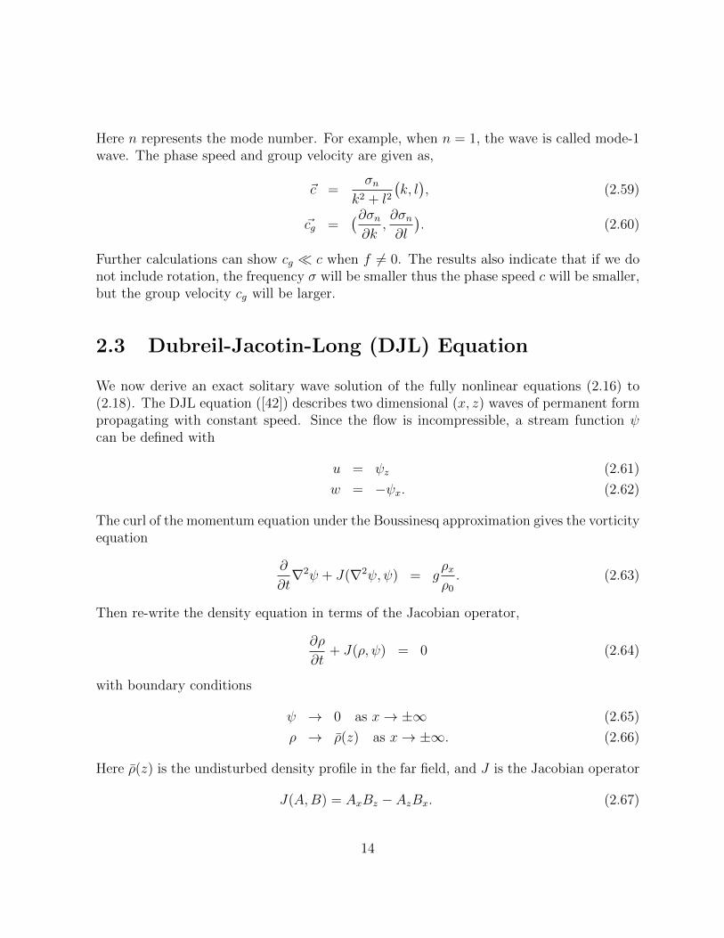
2.2 Phase speed vs wavenumber for the linearized equations with rotation. . . 11

2.3 Group velocity vs wavenumber for the linearized equations with rotation. . 12

3.1 Possible solution plots, η VS x, of the eKdV equation are presented. Thetop left plot is for α > 0, α1 > 0; the top right plot is for α < 0, α1 > 0;the bottom left plot is for α > 0, α1 < 0; the bottom right plot is for α < 0,α1 < 0. When α1 < 0, the wave flattens out as its amplitude approaches thelimit. The plots only show the qualitative behaviors of the solutions, thusthe grids are not displayed on the plots. . . . . . . . . . . . . . . . . . . . 31

3.2 Frequency vs wavenumber for the linearized KdV equation. . . . . . . . . . 33

3.3 Phase speed vs wavenumber and group velcoity vs wavenumber for the lin-earized KdV equation. . . . . . . . . . . . . . . . . . . . . . . . . . . . . . 33

3.4 Frequency vs wavenumber for the linearized Ostrovsky equation. . . . . . . 35

3.5 Phase speed vs wavenumber and group velocity vs wavenumber for the lin-earized Ostrovsky equation. . . . . . . . . . . . . . . . . . . . . . . . . . . 35

3.6 Frequency σ1 vs wavenumber for the linearized alternative form of Ostrovskyequation. . . . . . . . . . . . . . . . . . . . . . . . . . . . . . . . . . . . . . 37

3.7 Phase speed c1 vs wavenumber and group velocity cg1 vs wavenumber forthe linearized alternative form of Ostrovsky equation. . . . . . . . . . . . . 37

3.8 Frequency σ2 vs wavenumber for the linearized alternative form of Ostrovskyequation. . . . . . . . . . . . . . . . . . . . . . . . . . . . . . . . . . . . . . 38

3.9 Phase speed c2 vs wavenumber and group velocity cg2 vs wavenumber forthe linearized alternative form of Ostrovsky equation. . . . . . . . . . . . . 38

3.10 Frequency vs wavenumber. . . . . . . . . . . . . . . . . . . . . . . . . . . . 40

x

3.11 Phase speed vs wavenumber. . . . . . . . . . . . . . . . . . . . . . . . . . . 40

3.12 Group velocity vs wavenumber. . . . . . . . . . . . . . . . . . . . . . . . . 41

4.1 water depth vs density . . . . . . . . . . . . . . . . . . . . . . . . . . . . . 45

4.2 Solitary wave of depression. This is the wave solution of the eKdV equation. 47

4.3 Wave initialization for the alternative Ostrovsky equation. The spikes showthe locations of the initial wave of elevation and depression. . . . . . . . . 48

4.4 Time = 6000 s . . . . . . . . . . . . . . . . . . . . . . . . . . . . . . . . . 49

4.5 Time = 12000 s . . . . . . . . . . . . . . . . . . . . . . . . . . . . . . . . . 49

4.6 Time = 168000 s . . . . . . . . . . . . . . . . . . . . . . . . . . . . . . . . 49

4.7 Time = 240000 s . . . . . . . . . . . . . . . . . . . . . . . . . . . . . . . . 49

4.8 Initial wave profile . . . . . . . . . . . . . . . . . . . . . . . . . . . . . . . 50

4.9 Zoomed in view of the initial elevation . . . . . . . . . . . . . . . . . . . . 50

4.10 Time = 72000 s . . . . . . . . . . . . . . . . . . . . . . . . . . . . . . . . . 50

4.11 Time = 144000 s . . . . . . . . . . . . . . . . . . . . . . . . . . . . . . . . 50

4.12 Time = 216000 s . . . . . . . . . . . . . . . . . . . . . . . . . . . . . . . . 51

4.13 Time = 300000 s . . . . . . . . . . . . . . . . . . . . . . . . . . . . . . . . 51

4.14 Initial wave profile for the Ostrovsky equation . . . . . . . . . . . . . . . . 52

4.15 Zoomed in view of the initial elevation . . . . . . . . . . . . . . . . . . . . 52

5.1 Time = 600000 s. Results are from IGW simulation. Initial wave amplitudeis 79 m, and the plots show the vertical displacement of a isopycnal wherethe displacement is the greatest. . . . . . . . . . . . . . . . . . . . . . . . . 55

5.2 Time = 300000 s for the Ostrovsky solver. Plots show the vertical displace-ment of the isopycnal. . . . . . . . . . . . . . . . . . . . . . . . . . . . . . 56

5.3 Time = 600000 s for the Ostrovsky solver. Plots show the vertical displace-ment of the isopycnal. . . . . . . . . . . . . . . . . . . . . . . . . . . . . . 56

5.4 Time = 300000 s for the alternative Ostrovsky solver. . . . . . . . . . . . 57

5.5 Time = 600000 s for the alternative Ostrovsky solver. . . . . . . . . . . . 57

5.6 Time = 0s. The initial leading wave profile of Ostrovsky and alternativeOstrovsky solvers are exactly the same, so they coincide with each other.The initial waves of the IGW and the weakly nonlinear models are slightlydifferent, since IGW uses solitary wave solution of the DJL equation not theeKdV equation. . . . . . . . . . . . . . . . . . . . . . . . . . . . . . . . . . 58

xi

5.7 Time = 120000 s. . . . . . . . . . . . . . . . . . . . . . . . . . . . . . . . . 59

5.8 Time = 240000 s. . . . . . . . . . . . . . . . . . . . . . . . . . . . . . . . . 59

5.9 Time = 300000 s. . . . . . . . . . . . . . . . . . . . . . . . . . . . . . . . . 60

5.10 Time = 480000 s. . . . . . . . . . . . . . . . . . . . . . . . . . . . . . . . . 60

5.11 Time = 600000 s. . . . . . . . . . . . . . . . . . . . . . . . . . . . . . . . . 61

5.12 Initial wave profile . . . . . . . . . . . . . . . . . . . . . . . . . . . . . . . 62

5.13 Time = 120000 s. . . . . . . . . . . . . . . . . . . . . . . . . . . . . . . . . 63

5.14 Time = 240000 s. . . . . . . . . . . . . . . . . . . . . . . . . . . . . . . . . 63

5.15 Time = 300000 s. . . . . . . . . . . . . . . . . . . . . . . . . . . . . . . . . 64

5.16 Time = 480000 s. . . . . . . . . . . . . . . . . . . . . . . . . . . . . . . . . 64

5.17 Time = 600000 s. . . . . . . . . . . . . . . . . . . . . . . . . . . . . . . . . 65

5.18 Initial wave profile . . . . . . . . . . . . . . . . . . . . . . . . . . . . . . . 66

5.19 Time = 120000 s. . . . . . . . . . . . . . . . . . . . . . . . . . . . . . . . . 66

5.20 Time = 240000 s. . . . . . . . . . . . . . . . . . . . . . . . . . . . . . . . . 67

5.21 Time = 300000 s. . . . . . . . . . . . . . . . . . . . . . . . . . . . . . . . . 67

5.22 Time = 480000 s. . . . . . . . . . . . . . . . . . . . . . . . . . . . . . . . . 68

5.23 Time = 600000 s. . . . . . . . . . . . . . . . . . . . . . . . . . . . . . . . . 68

5.24 Frequency vs wavenumber for the linearized equations. A small range of kvalues are plotted here, since only these values will be needed in the lateranalysis. . . . . . . . . . . . . . . . . . . . . . . . . . . . . . . . . . . . . . 70

5.25 Phase speed vs wavenumber for the linearized equations. . . . . . . . . . . 71

5.26 Group velocity vs wavenumber for the linearized equations. . . . . . . . . . 71

5.27 Phase speed vs wavenumber for the linearized equations. . . . . . . . . . . 73

5.28 Group velocity vs wavenumber for the linearized equations. . . . . . . . . . 74

5.29 Frequency vs wavenumber for the linearized equations. A smaller range fork, i.e. [6e-5, 2e-4] m−1, is plotted here to have a clear view to the changesof the frequencies. . . . . . . . . . . . . . . . . . . . . . . . . . . . . . . . . 74

5.30 Frequency vs wavenumber for the linearized equations. The plot on the lefthas a range of k as [1e-5, 1e-2] m−1; the plot on the right has a range of kas [1e-5, 5e-3] m−1. The plots for LO are not observable since they almostcoincide with the plots for LAO. . . . . . . . . . . . . . . . . . . . . . . . . 75

xii

5.31 Phase speed vs wavenumber for the linearized equations. The plot on theleft has a range of k as [1e-5, 1e-2] m−1; the plot on the right has a range ofk as [1e-5, 5e-3] m−1. The plots for LO are not observable since they almostcoincide with the plots for LAO. . . . . . . . . . . . . . . . . . . . . . . . . 75

5.32 Group velocity vs wavenumber for the linearized equations. The plot on theleft has a range of k as [1e-5, 1e-2] m−1; the plot on the right has a range ofk as [1e-5, 5e-3] m−1. The plots for LO are not observable since they almostcoincide with the plots for LAO. . . . . . . . . . . . . . . . . . . . . . . . . 76

5.33 |c − cg| vs wavenumber for the linearized equations. The plot on the lefthas a range of k as [1e-5, 1e-2] m−1; the plot on the right has a range of kas [1e-5, 2e-4] m−1. The plot for LO on the left hand side is not observablesince it almost coincides with the plot for LAO. . . . . . . . . . . . . . . . 76

xiii

Chapter 1

Introduction

1.1 Observations and Importance of Internal Waves

Internal waves (IWs) are waves that propagate in the interior of a density stratified fluidunder the influence of gravitational restoring forces. For example, these waves can be seenfrom the visible oscillations in two-layer immiscible colored fluids of different density in atransparent plastic box. The occurrence of this wave is due to the different densities ofthe two fluids, especially the discrete density change across the interface. The larger thedensity difference the larger the wave frequency for a given wavelength.

The common occurrence of solitary waves in the ocean has been widely accepted. JohnScott Russell (1838, 1844) seemed to be the first one who documented the observation ofsurface solitary waves in the shallow water of the Union canal in Scotland. Following Rus-sell, some other observations of solitary waves were made by Wallace (1869). The solitarywave solutions of the surface waves were found in 1871 and 1876, and the KdV equation wasderived in 1895. More details of the solitons will be mentioned later in the next subsection.Some later observations of solitary waves include Fu and Holt (1982), Apel and Gonzales(1984), Apel et al. (1985) and Liu et al. (1985). In 1965, Perry & Schimke’s measurementsdetected groups of internal waves up to 80m high and 2000m long in the Andaman Sea.Due to the development of the ocean instrumentation and remote sensors, many signifi-cant observations were made in the 1970s, such as, Halpern (1971) in Massachusetts Bay,Thorpe (1971) and Hunkins & Fliegel (1973) in Loch Ness and Seneca Lake, New York.Meanwhile, Ziegenbein (1969, 1970) made similar observations in the Strait of Gibraltar,which provided clear evidence of the ISWs. Apel et al. (1975) reported the occurrenceof internal solitray waves (ISWs) in the New York Bight based on the collective data in1972 and 1973. More examples about the observations of ISWs can be found in the secondedition of the Atlas of Oceanic Internal Solitary Waves, where around 300 cases from 54

1

regions over the world are listed.

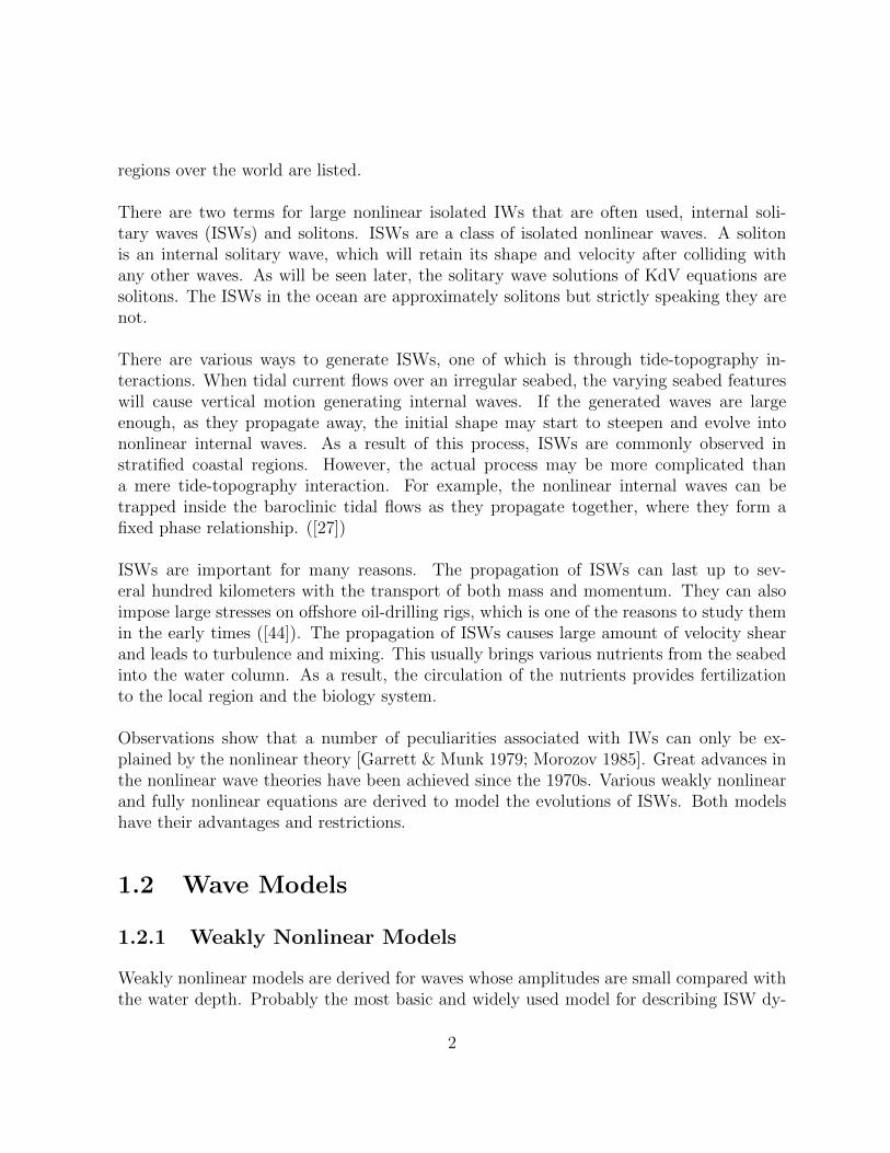
There are two terms for large nonlinear isolated IWs that are often used, internal soli-tary waves (ISWs) and solitons. ISWs are a class of isolated nonlinear waves. A solitonis an internal solitary wave, which will retain its shape and velocity after colliding withany other waves. As will be seen later, the solitary wave solutions of KdV equations aresolitons. The ISWs in the ocean are approximately solitons but strictly speaking they arenot.

There are various ways to generate ISWs, one of which is through tide-topography in-teractions. When tidal current flows over an irregular seabed, the varying seabed featureswill cause vertical motion generating internal waves. If the generated waves are largeenough, as they propagate away, the initial shape may start to steepen and evolve intononlinear internal waves. As a result of this process, ISWs are commonly observed instratified coastal regions. However, the actual process may be more complicated thana mere tide-topography interaction. For example, the nonlinear internal waves can betrapped inside the baroclinic tidal flows as they propagate together, where they form afixed phase relationship. ([27])

ISWs are important for many reasons. The propagation of ISWs can last up to sev-eral hundred kilometers with the transport of both mass and momentum. They can alsoimpose large stresses on offshore oil-drilling rigs, which is one of the reasons to study themin the early times ([44]). The propagation of ISWs causes large amount of velocity shearand leads to turbulence and mixing. This usually brings various nutrients from the seabedinto the water column. As a result, the circulation of the nutrients provides fertilizationto the local region and the biology system.

Observations show that a number of peculiarities associated with IWs can only be ex-plained by the nonlinear theory [Garrett & Munk 1979; Morozov 1985]. Great advances inthe nonlinear wave theories have been achieved since the 1970s. Various weakly nonlinearand fully nonlinear equations are derived to model the evolutions of ISWs. Both modelshave their advantages and restrictions.

1.2 Wave Models

1.2.1 Weakly Nonlinear Models

Weakly nonlinear models are derived for waves whose amplitudes are small compared withthe water depth. Probably the most basic and widely used model for describing ISW dy-

2

namics is the Korteweg-de Vries (KdV) equation. The history of the KdV equation beganwith John Russell’s experiment in 1834, followed by Boussinesq and Rayleigh, who foundthe solitary wave solution independently in 1871 and 1876. Then in 1895, Diederik Ko-rteweg and his student Gustav de Vries derived the KdV equation, which describes weaklynonlinear, long and unidirectional surface water waves. Followed by this original work,Zabusky & Kruskal (1965) discovered the soliton solution, and later a cubic nonlinear termwas added to incorporate higher-order nonlinear effects. This equation is known as eKdVor Gardner equation, which can deal with waves of larger amplitudes compared with theclassic KdV equation. When applied to the internal solitons, KdV type theories providequite satisfactory results as well, even though there are many other solitary wave equa-tions derived after this. Other weakly nonlinear internal wave theories for different scalesinclude, a model developed by Benjamin (1967) and Ono (1975) for infinitely deep fluids,and a model derived by Joseph (1977) and Kubota et al. (1978) for intermediate depth.

Maxworthy (1983) pointed out that in some instances the effects of the Earths rotation can-not be ignored. The effects of rotation may be comparable to weak nonlinear and dispersiveeffects. Ostrovsky (1978) firstly extended the unidirectional KdV equation to include theeffects of weak rotation on nonlinear dispersive internal waves. The resulting equation isknown as the Ostrovsky equation and many conservation laws have been derived from it.There are no solitary wave solutions of the Ostrovsky equation. If we use solitary solutionsof the KdV as the initial condition for the Ostrovsky equation, the solitary wave will de-cay in time and its energy will slowly be diverted to an inertia-gravity wave train due torotational effects. Numerical studies of the Ostrovsky equation have shown an interestingphenomenon: the wave train can steepen up and form a second solitary-like wave behindthe leading solitary wave. This second solitary-like wave can then decay and this wholeprocess may repeat and lead to more solitary-like waves in the wave train ([48]). ModelingISWs with weak rotational effects is the focus of this thesis.

Many simulations have been run to model internal waves with rotational effects. Holloway& Pelinovsky & Talipova (1999) used the Gardner-Ostrovsky equation with a dissipationterm to model evolutions of the shoaling internal tides observed on the north west shelf(NWS) of Australia. Numerical results were compared with the observations on the NWS.The paper shows that rotation is important for modeling internal waves even for low lat-itude regions. Helfrich (2007) used a fully nonlinear, weakly nonhydrostatic theory, i.e.MCC theory, to model the propagation of ISWs. Grimshaw & Pelinovsky & Stepanyants& Talipova (2006) used the Gardner-Ostrovsky equation to model ISWs on the NWS.Both depth variation and horizontal variability of the stratification were considered in themodel. Johnson & Grimshaw (2013) and Grimshaw & Helfrich & Johnson (2012) used areduced modified Ostrovsky equation, where the linear dispersive term and the quadraticterm have been set to 0, to determine the constraint for wave breaking. They show that the

3

reduced Ostrovsky equation is integrable given certain slope constraints. Here, equationswith an infinite number of integrals of motion in involution are called integrable. ([1])Wave breaking can occur if the constraint is not satisfied. Grimshaw & Helfrich (2008) rana long-time numerical simulation of the Ostrovsky equation to show that a localized wavepacket emerged as a persistent feature.

Since ISWs are usually observed around varying or steep topography in the ocean, such ascoastal regions, recently various of KdV-type equations have been developed to incorporatethe effects of shoaling. As such, the coefficients of the KdV equations change with the vary-ing topography. Lamb (2002, 2003) simulated behaviors of waves shoaling over changingtopography, and then further explored the relations of the configuration of the shoalingwaves and the limiting form of the corresponding solitary waves. There will not be anytrapped cores if the limiting form of the ISWs includes a conjugate flow. Here, a conjugateflow refers to the horizontally uniform flow that is in the center of long flat waves [Benjamin(1996); Mehrotra & Kelly (1973); Lamb & Wan 1998]. Grue el al. (2000) found that a corecan be formed if the limiting form corresponds to the maximum horizontal velocity in thewave matching the wave speed. However, this thesis only considers waves propagating on aflat bottom and all the coefficients of the KdV theories are constant through space and time.

There are other extensions of the KdV equations. The KdV equation can be extendedto account for weak two-dimensionality, i.e., two horizontal dimensions x and y with avertical scale z. The resulting equation is called the Kadomtsev and Petviashvili (1970,KP) equation. Pierini (1989) used the KP equation to simulate the waves in the Strait ofGibraltar, and the implementation was done by Chen and Liu (1995).

Laboratory experiments have been conducted to investigate and compare the validity ofweakly nonlinear models. Koop & Butler (1981) and Segur & Hammack (1982) showed thatKdV performs quantitatively better than the Benjamin-Ono equation, for weakly nonlinearwaves in deep water. Through some two-layer fluid experiment with h1

h2= 0.24, Grue et al.

(1999) showed that KdV theory can model wave with amplitudes up to η0h1≈ 0.4, but it

does not manage to capture the broadening of ISWs with increasing amplitudes. Michallet& Barthelemy (1998) noticed improvements from eKdV. In their two-layer experiment for0.4 < h1

h1+h2< 0.6, prediction of eKdV equation matches excellent with the lab results.

1.2.2 Fully Nonlinear Models

In contrast with the weakly nonlinear models, fully nonlinear models make fewer sim-plifications, thus they are a more accurate set of equations. As a result, there are norestrictions when applying the fully nonlinear models. For example, the wave amplitude

4

does not need to be small as that in the KdV-type equations. Fully nonlinear models showbetter results than the weakly nonlinear models as well. However, the disadvantages arethat solving these models are usually more time-consuming and expensive ([17]). Hence,it is very important to develop and improve weakly nonlinear models so that they canproduce comparable results as the fully nonlinear models do, while being more efficientand cheaper. However, we can only expect the weakly nonlinear models to perform wellwithin a restricted set of phenomena, since they have many limitations and each weaklynonlinear equation has its validity range.

Laboratory experiments have also been conducted to check the fully nonlinear model.For example, Michallet & Barthelemy (1998) and Grue et al. (1999) found nice agreementof the fully nonlinear two-layer model and their laboratory measurements of an ISW overa broad range of relative layer depths.

1.3 Thesis Structure and Goals

Some brief background information about the fully nonlinear equations with Earth’s ro-tation will be mentioned in Chapter 2. Derivations and solution analysis of the weaklynonlinear equations, i.e., the alternative Ostrovsky equation, the Ostrovsky equation andKdV-type equations, will be covered in Chapter 3. Numerical models and the correspond-ing simulation results will be illustrated in Chapter 4 and 5. Conclusions and summarywill be in the last chapter.

A new equation, i.e., the alternative Ostrovsky equation, has been introduced. The goalof this thesis is to compare this new equation with the existing Ostrovsky equation, andfurther compare them with the fully nonlinear model through numerical simulations.

5

Chapter 2

Theoretical Background

2.1 Fully Nonlinear Equations with Rotation

This thesis considers a fluid that is stratified, incompressible, inviscid and non-diffusive,moving in a rotating-reference frame. The momentum equations, as a result of Newton’ssecond law, are

ρ(D~U

Dt+ 2~Ω× ~U) = − ~∇p− ρgk. (2.1)

Here u, v and w are the velocity at x, y and z direction respectively; ~U = (u, v, w);p is the pressure of the fluid; ρ is the density of the fluid; g is the acceleration due togravity; k = (0, 0, 1) is the unit vector in the vertical direction, and f is the Coriolisparameter associated with the Earth’s rotation. The notation D

Dtis the material derivative,

representing the rate of change moving with a fluid particle. It is defined as,

D

Dt=

∂

∂t+ ~U · ~∇. (2.2)

2.1.1 f-plane Approximation

In the momentum equation (2.1), ~Ω = (Ωx,Ωy,Ωz) = (0,Ω cos θ,Ω sin θ) is the angularvelocity of the Earth in the local Cartesian system. The Earth rotates at Ω = 2π rad/day =0.73× 10−4 s−1 and θ is the latitude. f is defined to be 2Ω sin θ and f is usually referredto as the Coriolis parameter or the Coriolis frequency. We can note that the full Coriolisterm is of the following form,

2~Ω× ~U = (−fv + 2Ωw cos θ, fu,−2Ωu cos θ). (2.3)

6

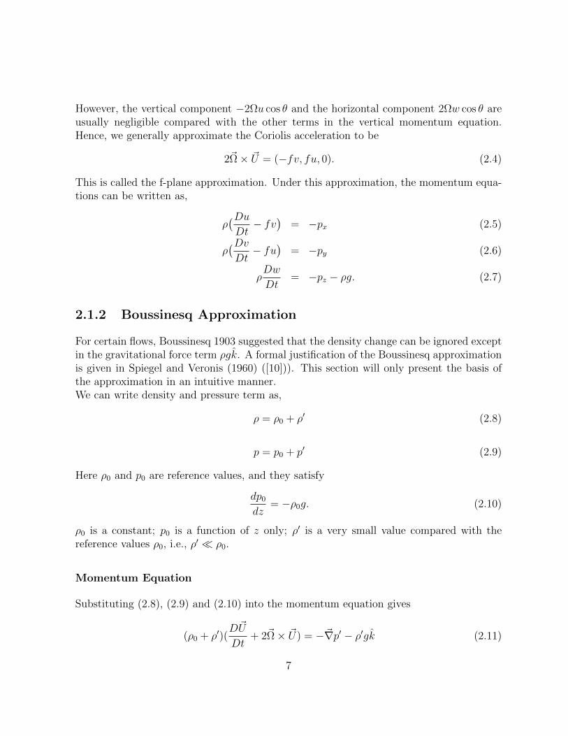
However, the vertical component −2Ωu cos θ and the horizontal component 2Ωw cos θ areusually negligible compared with the other terms in the vertical momentum equation.Hence, we generally approximate the Coriolis acceleration to be

2~Ω× ~U = (−fv, fu, 0). (2.4)

This is called the f-plane approximation. Under this approximation, the momentum equa-tions can be written as,

ρ(DuDt− fv

)= −px (2.5)

ρ(DvDt− fu

)= −py (2.6)

ρDw

Dt= −pz − ρg. (2.7)

2.1.2 Boussinesq Approximation

For certain flows, Boussinesq 1903 suggested that the density change can be ignored exceptin the gravitational force term ρgk. A formal justification of the Boussinesq approximationis given in Spiegel and Veronis (1960) ([10])). This section will only present the basis ofthe approximation in an intuitive manner.We can write density and pressure term as,

ρ = ρ0 + ρ′ (2.8)

p = p0 + p′ (2.9)

Here ρ0 and p0 are reference values, and they satisfy

dp0

dz= −ρ0g. (2.10)

ρ0 is a constant; p0 is a function of z only; ρ′ is a very small value compared with thereference values ρ0, i.e., ρ′ ρ0.

Momentum Equation

Substituting (2.8), (2.9) and (2.10) into the momentum equation gives

(ρ0 + ρ′)(D~U

Dt+ 2~Ω× ~U) = −~∇p′ − ρ′gk (2.11)

7

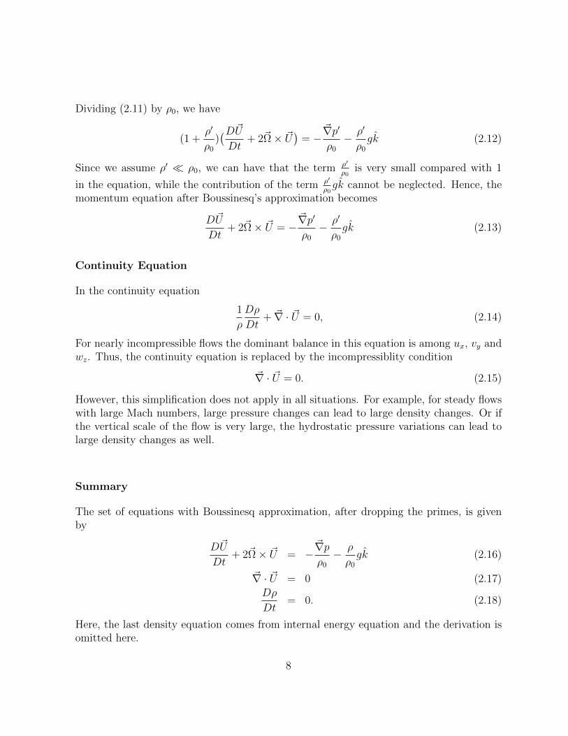
Dividing (2.11) by ρ0, we have

(1 +ρ′

ρ0

)(D~UDt

+ 2~Ω× ~U)

= −~∇p′

ρ0

− ρ′

ρ0

gk (2.12)

Since we assume ρ′ ρ0, we can have that the term ρ′

ρ0is very small compared with 1

in the equation, while the contribution of the term ρ′

ρ0gk cannot be neglected. Hence, the

momentum equation after Boussinesq’s approximation becomes

D~U

Dt+ 2~Ω× ~U = −

~∇p′

ρ0

− ρ′

ρ0

gk (2.13)

Continuity Equation

In the continuity equation

1

ρ

Dρ

Dt+ ~∇ · ~U = 0, (2.14)

For nearly incompressible flows the dominant balance in this equation is among ux, vy andwz. Thus, the continuity equation is replaced by the incompressiblity condition

~∇ · ~U = 0. (2.15)

However, this simplification does not apply in all situations. For example, for steady flowswith large Mach numbers, large pressure changes can lead to large density changes. Or ifthe vertical scale of the flow is very large, the hydrostatic pressure variations can lead tolarge density changes as well.

Summary

The set of equations with Boussinesq approximation, after dropping the primes, is givenby

D~U

Dt+ 2~Ω× ~U = −

~∇pρ0

− ρ

ρ0

gk (2.16)

~∇ · ~U = 0 (2.17)

Dρ

Dt= 0. (2.18)

Here, the last density equation comes from internal energy equation and the derivation isomitted here.

8

2.2 Linearized Equations

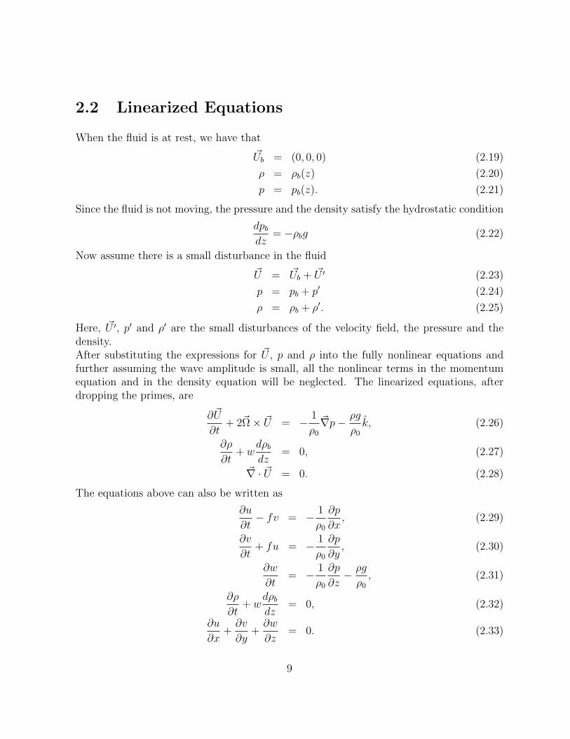
When the fluid is at rest, we have that

~Ub = (0, 0, 0) (2.19)

ρ = ρb(z) (2.20)

p = pb(z). (2.21)

Since the fluid is not moving, the pressure and the density satisfy the hydrostatic condition

dpbdz

= −ρbg (2.22)

Now assume there is a small disturbance in the fluid

~U = ~Ub + ~U ′ (2.23)

p = pb + p′ (2.24)

ρ = ρb + ρ′. (2.25)

Here, ~U ′, p′ and ρ′ are the small disturbances of the velocity field, the pressure and thedensity.After substituting the expressions for ~U , p and ρ into the fully nonlinear equations andfurther assuming the wave amplitude is small, all the nonlinear terms in the momentumequation and in the density equation will be neglected. The linearized equations, afterdropping the primes, are

∂~U

∂t+ 2~Ω× ~U = − 1

ρ0

~∇p− ρg

ρ0

k, (2.26)

∂ρ

∂t+ w

dρbdz

= 0, (2.27)

~∇ · ~U = 0. (2.28)

The equations above can also be written as

∂u

∂t− fv = − 1

ρ0

∂p

∂x, (2.29)

∂v

∂t+ fu = − 1

ρ0

∂p

∂y, (2.30)

∂w

∂t= − 1

ρ0

∂p

∂z− ρg

ρ0

, (2.31)

∂ρ

∂t+ w

dρbdz

= 0, (2.32)

∂u

∂x+∂v

∂y+∂w

∂z= 0. (2.33)

9

2.2.1 Buoyancy Frequency

We introduce the definition for the buoyancy frequency N here. It is defined by

N2(z) = − g

ρ0

dρbdz

. (2.34)

Equation (2.32) can be written as

∂ρ

∂t− wN

2ρ0

g= 0. (2.35)

The importance of N(z) in stratified flows will be discussed in the next section.

2.2.2 Constant N

Firstly, the linear stratification, i.e. constant N, is considered here, since we want to findanalytic expression for the dispersion relation. Assume a plane wave solution

u = u0ei(kx+ly+mz−σt), (2.36)

v = v0ei(kx+ly+mz−σt), (2.37)

w = w0ei(kx+ly+mz−σt), (2.38)

p = p0ei(kx+ly+mz−σt), (2.39)

ρ = ρ0ei(kx+ly+mz−σt). (2.40)

Substituting these expressions into (2.29) to (2.33), we obtain the dispersion relation,

σ2 =N2k2 + f 2m2

k2 +m2, (2.41)

where l has been set to be 0. The result indicates that if we do not include rotation, thefrequency, the phase speed and the group velocity will be smaller. The first set of figuresis of the frequency σ; the second set of figures is of the phase speed c and the third set offigures is of the group velocity cg. All of them are plotted as functions of wavenumber k.For mode-one waves, using f = 10−4 s−1, H = 3 km and N = 10−3 s−1, hence

m =π

H=

π

3000. (2.42)

10

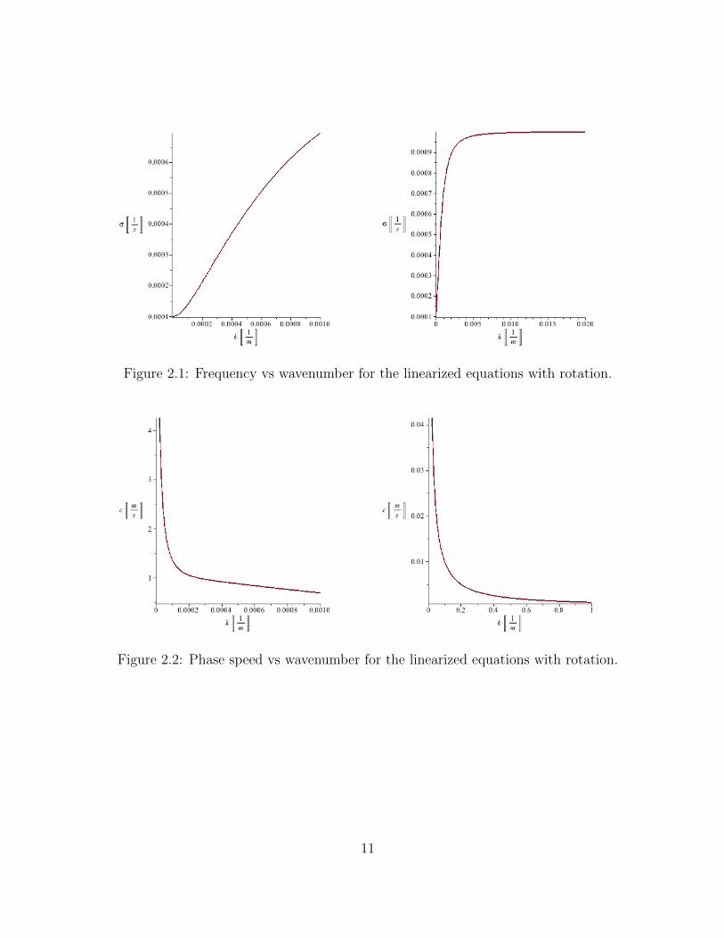
Figure 2.1: Frequency vs wavenumber for the linearized equations with rotation.

Figure 2.2: Phase speed vs wavenumber for the linearized equations with rotation.

11

Figure 2.3: Group velocity vs wavenumber for the linearized equations with rotation.

From the dispersion relation,

σ ∼

f as k → 0

N as k →∞.(2.43)

c =σ

k∼

fk

as k → 0Nk

as k →∞.(2.44)

cg =∂σ

∂k∼

(N2−f2)fm2 k as k → 0

m2(N2−f2)N

1k3

as k →∞.(2.45)

As the wave becomes infinitely long, k → 0, the frequency of the wave goes to f , the phasespeed c goes to infinity and the group velocity cg goes to 0.

2.2.3 Non-constant N

Secondly, we consider the case when the stratification is not linear, i.e., N = N(z). Anequation for w can be obtained from eliminating all the other variables in (2.29) to (2.33).

∂2

∂t2∇2w +N2∇2

Hw + f 2∂2w

∂z2= 0, (2.46)

12

where ∇2 = ∂2

∂x2+ ∂2

∂y2+ ∂2

∂z2and ∇2

H = ∂2

∂x2+ ∂2

∂y2. Now we assume the solutions have the

following form,

u = u0(z)ei(kx+ly−σt), (2.47)

v = v0(z)ei(kx+ly−σt), (2.48)

w = φ(z)ei(kx+ly−σt), (2.49)

p = p0(z)ei(kx+ly−σt), (2.50)

ρ = ρ0(z)ei(kx+ly−σt). (2.51)

Substituion into the w-equation (2.46) gives

d2φ

dz2+

(N2 − σ2)(k2 + l2)

σ2 − f 2φ = 0. (2.52)

Defining

m2(z) =(N2 − σ2)(k2 + l2)

σ2 − f 2, (2.53)

(2.52) becomes

d2φ

dz2+m2φ = 0. (2.54)

Now we impose the rigid-lid approximation, which is used throughout this thesis. Thereis no solution satisfying (2.54) and the rigid-lid approximation when m2 < 0 everywhere,thus we only consider the fluid layer where m2 > 0. Following this argument, we have

f < σ < N. (2.55)

Rayleigh gives the solution for the particular case when N is constant.

φ = sin(m(z +H)

). (2.56)

Here H is the water depth; mH = nπ, where n is any positive integer. This solution canbe viewed as linear combination of the solutions from the constant N case, since

sin(m(z +H)

)=

1

2

(ei(m(z+H)) − e−i(m(z+H))

). (2.57)

Following the Rayleigh solution, we can get the dispersion relation,

σ2n =

(k2 + l2)N2H2 + f 2n2π2

n2π2 + (k2 + l2)H2. (2.58)

13

Here n represents the mode number. For example, when n = 1, the wave is called mode-1wave. The phase speed and group velocity are given as,

~c =σn

k2 + l2(k, l), (2.59)

~cg =(∂σn∂k

,∂σn∂l

). (2.60)

Further calculations can show cg c when f 6= 0. The results also indicate that if we donot include rotation, the frequency σ will be smaller thus the phase speed c will be smaller,but the group velocity cg will be larger.

2.3 Dubreil-Jacotin-Long (DJL) Equation

We now derive an exact solitary wave solution of the fully nonlinear equations (2.16) to(2.18). The DJL equation ([42]) describes two dimensional (x, z) waves of permanent formpropagating with constant speed. Since the flow is incompressible, a stream function ψcan be defined with

u = ψz (2.61)

w = −ψx. (2.62)

The curl of the momentum equation under the Boussinesq approximation gives the vorticityequation

∂

∂t∇2ψ + J(∇2ψ, ψ) = g

ρxρ0

. (2.63)

Then re-write the density equation in terms of the Jacobian operator,

∂ρ

∂t+ J(ρ, ψ) = 0 (2.64)

with boundary conditions

ψ → 0 as x→ ±∞ (2.65)

ρ → ρ(z) as x→ ±∞. (2.66)

Here ρ(z) is the undisturbed density profile in the far field, and J is the Jacobian operator

J(A,B) = AxBz − AzBx. (2.67)

14

We are interested in rightward propagating waves with constant phase speed c that main-tain their shapes while they travel, i.e., solutions of the form

ψ(x, z, t) = ψ(x− ct, z) (2.68)

ρ(x, z, t) = ρ(x− ct, z). (2.69)

Using these, (2.63) and (2.64) become

J(∇2ψ, ψ − cz) = gρxρ0

, (2.70)

J(ρ, ψ − cz) = 0. (2.71)

Equation (2.71) indicates that ρ and ψ− cz are functionally related, which can be writtenas

ρ = F (ψ − cz) (2.72)

for some function F . Using the far field boundary condition when x→ ±∞

F (ψ − cz) → F (−cz), (2.73)

ρ → ρ(z), (2.74)

hence

F (−cz) = ρ(z) ⇒ F (z) = ρ(−zc

). (2.75)

Now we define a function ζ(x, z) as the vertical displacement of the streamline passingthrough the point (x, z). Then the density profile can be related to the far-field unperturbeddensity field via

ρ(x, z) = ρ(z − ζ(x, z)). (2.76)

Combined with the function F , we have

ρ = F (ψ − cz) = ρ(z − ψ

c) = ρ(z − ζ), (2.77)

which implies that

ψ(x, z) = cζ(x, z). (2.78)

Substitution of the equality (2.78) into the equation (2.70) and expanding ρx gives

J(c∇2ζ, cζ − cz) = gρxρ0

= N2(z − ζ)ζx, (2.79)

15

where (2.76) has been used for the last step. Since ζx = J(ζ, z) = J(ζ, z − ζ), we canfurther write the right hand side of (2.79) as

N2(z − ζ)J(ζ, z − ζ) = J(N2(z − ζ)ζ, z − ζ). (2.80)

Then (2.79) can again be written as

J(∇2ζ +

N2(z − ζ)

c2ζ, ζ − z

)= 0. (2.81)

Hence, ∇2ζ + N2(z−ζ)c2

ζ and ζ − z are functionally related, i.e.,

∇2ζ +N2(z − ζ)

c2ζ = G(ζ − z) (2.82)

for some function G. Imposing the far field boundary condition

ζ → 0 as x→ ±∞, (2.83)

gives G(z) = 0. Thus,

∇2ζ +N2(z − ζ)

c2ζ = 0. (2.84)

This is the Dubreil-Jacotin-Long (DJL) equation ([42]). From the derivation of the DJLequation, we can see that this equation is for waves with open streamlines. Open stream-lines are streamlines that come from the far field and are not closed. However, this equationcan be applied to closed streamlines as well, except that it is indeterminate.

16

Chapter 3

Weakly Nonlinear Equations

Fully nonlinear numerical models are usually time consuming and expensive to solve, al-though they can be very accurate and can be applied to waves of arbitrary amplitude.Weakly-nonlinear models can be a very efficient substitute. The focus of this section is onKdV-type equations, which have been widely used and which are appropriate under thesmall and long wave assumptions.

3.1 Derivation of the Ostrovsky Equation

The incompressibility condition and the fact that we are looking for solutions independentof y leads us to a scalar stream function formulation. Then we start with the governingequations (2.16) to (2.18) derived in Chapter 2, and follow a procedure similar to that usedin the derivation of the vorticity equation in the section 2.3. The equations become

∂

∂t∇2ψ + J(∇2ψ, ψ) = g

ρxρ0

+ fvz (3.1)

vt + fψz = J(ψ, v) (3.2)

∂ρ

∂t+ J(ρ, ψ) = 0, (3.3)

where (u,w) = (ψz,−ψx). This set of equations is often referred to as a 2.5 dimensionmodel since v can be non-zero. We assume that the unperturbed state is a state of restwith stratification ρ = ρ(z) so that

ρ = ρ(z) + ρ′(x, z, t). (3.4)

Defining

b =gρ′

ρ0

, (3.5)

17

the equations can be written as

∂

∂t∇2ψ + J(∇2ψ, ψ) = bx + fvz (3.6)

vt + fψz = J(ψ, v) (3.7)

∂b

∂t+N2(z)ψx = J(ψ, b). (3.8)

3.1.1 Boundary Conditions

To focus on internal waves we make the rigid lid approximation which eliminates surfacewaves, which also indicates there is no density perturbation on the top and bottom. Wealso assume that as x→∞, the water is undisturbed and at rest so that u→ 0. Thus, wehave

ψ = b = 0 at z = −H, 0 (3.9)

ψ, b → 0 as x→∞. (3.10)

3.1.2 Non-dimensionalization

The spatial coordinates and buoyancy frequency are scaled as

x = Lx (3.11)

u = Uu (3.12)

w = Ww (3.13)

z = Hz (3.14)

N(z) = N0N(z), (3.15)

where L is a typical wavelength, W is the vertical velocity scale, H is the water depth andN0 is the typical value of N(z). The vertical structure function, which will appear later inthe derivation, is determined from the eigenvalue problem

φ′′ +N2

c20

φ = 0, (3.16)

here the eigenvalue c0 is the linear, long-wave speed and φ(z) gives the leading order verticalstructure of the wave. Under the change of variables z = Hz, (3.16) becomes

φ′′ +N2H2

c20

φ = 0. (3.17)

18

This indicates that c0 ∼ NH, thus we can choose the velocity and time scale to be

c = N0H (3.18)

T =L

c=

L

N0H(3.19)

We assume that the amplitude perturbation is small compared to the unperturbed state,i.e., the horizontal velocity u of the wave is small compared with the linear propagationspeed. By letting U = εc, we have

u = εcu = εN0Hu. (3.20)

Here ε is a small amplitude parameter. Now we set

ψ = εΨψ, (3.21)

Using u = ψz, we have

ψz = εN0Hu =εΨ

Hψz. (3.22)

This gives us that

Ψ = εN0H2. (3.23)

From the incompressibility condition ux + wz = 0 we see that

W =H

LU = ε

N0H2

L. (3.24)

We also need to scale b so we set b = Bb. Since we assume the perturbation is small, thetwo linear terms on the left hand side of equation (3.8) dominate. As a result, we need

b = εN20Hb. (3.25)

Now after substituting all these scaled variables and dropping the tildes, the governingequations (3.6) to (3.8) become

∂

∂tψzz − bx = εJ(ψ, ψzz)− µ

∂

∂tψxx + εµJ(ψ, ψxx) + δvz (3.26)

vt + ψz = εJ(ψ, v) (3.27)

∂

∂tb+N2(z)ψx = εJ(ψ, b), (3.28)

where µ =(HL

)2, ε can be viewed as a

H, δ = f2L2

c2is the inverse square of the Rossby number

and a is a typical wave amplitude. For all the scaling and the following derivations, weassume H L and a H, i.e., ε 1, µ 1 and δ 1.

19

3.1.3 Asymptotic Expansion

Since we have three small parameters ε, µ and δ, we can expand ψ and b as an asymptoticseries:

ψ ∼ ψ(0) + εψ(1,0,0) + µψ(0,1,0) + δψ(0,0,1) + h.o.t, (3.29)

b ∼ b(0) + εb(1,0,0) + µb(0,1,0) + δb(0,0,1) + h.o.t, (3.30)

v ∼ v(0) + εv(1,0,0) + µv(0,1,0) + δv(0,0,1) + h.o.t, (3.31)

where h.o.t. stands for higher order terms. We assume ψ(0) is separable as we are interestedin horizontally propagating waves, so that

ψ(0) = η(x, t)φ(z). (3.32)

Since the wave will change its shape while propagating, we will find that

ηt ∼ −c0ηx − εR(x, t)− µQ(x, t)− δT (x, t) + ε2S(x, t) + h.o.t.. (3.33)

Here, and in the following, by asymptotic we mean as ε, µ and δ all go to 0, η satisfies(3.33). For the derivation below, we set x0 to be the left boundary and t0 to be the initialtime.

O(1) problem:

The leading-order equations are

∂

∂tψ(0)zz − b(0)

x = 0 (3.34)

v(0)t + ψ(0)

z = 0 (3.35)

∂b(0)

∂t+N2(z)ψ(0)

x = 0. (3.36)

Using the leading-order part of (3.33), we have

φ′′ +N2(z)

c20

φ = 0 (3.37)

v(0)t = −ψ(0)

z = −η(x, t)φ′(z) (3.38)

b(0) =η

c0

N2(z)φ(z) = − ηc0

φ′′, (3.39)

where c0 is a constant. Equation (3.37) is an eigenvalue problem for φ and c0. The velocityin the y direction has the form

v(0) = G(x, t)φ′(z) (3.40)

20

where, from (3.38),

G(x, t) = G(x, t0)−∫ t

t0

η(x, t′)dt′. (3.41)

Here G(x, t0) is to be determined.

O(ε) problem:

The O(ε) equations are

−Rφ′′ + ∂

∂tψ(1,0,0)zz − b(1,0,0)

x = ηηx(φφ′′′ − φ′φ′′) (3.42)

−N2

c0

Rφ+∂

∂tb(1,0,0) +N2φ(1,0,0)

x = −c0ηηx(φφ′′′ − φ′φ′′). (3.43)

The v equation is not included here, since the two equations above do not involve v. Weagain look for separable solutions. The form of the nonlinear term on the right hand sidesuggests that we seek solutions of the form

ψ(1,0,0) = η2φ(1,0,0)(z) (3.44)

b(1,0,0) = η2D(1,0,0)(z) (3.45)

R = αηηx. (3.46)

Thus the equation (3.42) becomes

φ(1,0,0)zz +

N2

c20

φ(1,0,0) = − αc0

φ′′ − 1

c0

(φφ′′′ − φ′φ′′). (3.47)

If we multiply the left hand side of the equation by φ and integrate it from 0 to 1, the resultequals 0 and this solvability condition is used to calculate the coefficients in this derivation.Hence, imposing the condition that the integral of the right hand side multiplied by φ shouldalso equal to 0, we have the value for α,

α =3

2

∫ 0

−1φ′3dz∫ 0

−1φ′2dz

. (3.48)

O(µ) problem:

Following a similar procedure for the O(µ) problem, we find that

Q = βηxxx, (3.49)

β =c0

2

∫ 0

−1φ2dz∫ 0

−1φ′2dz

. (3.50)

Note that β > 0.

21

O(δ) Problem

Proceeding as in the previous cases, we have the following governing equations.

∂

∂tψ(0,0,1)zz − b(0,0,1)

x = v(0)z + T (x, t)

N2

c2φ (3.51)

b(0,0,1)t +N2ψ(0,0,1)

x = −T (x, t)N2

c0

φ(z) (3.52)

Here T (x, t) comes from the equation (3.33). The equation for v(0,0,1) is not of interest hereand we shall see later that it is not necessary to find v(0,0,1), so it is omitted. Again weassume the solutions are separable.

ψ(0,0,1) = η(0,0,1)(x, t)φ(0,0,1)(z), (3.53)

b(0,0,1) = η(0,0,1)(x, t)D(0,0,1)(z). (3.54)

Then we use the expression for v(0), which is derived in the O(1) problem. Equations (3.51)and (3.52) become,

η(0,0,1)t φ(0,0,1)

zz − η(0,0,1)x D(0,0,1) =

(T −G

)N2

c2φ, (3.55)

η(0,0,1)t D(0,0,1) +N2η(0,0,1)

x φ(0,0,1) = −T N2

c0

φ. (3.56)

From here, we assume that η(0,0,1)t , η

(0,0,1)x and T are proportional to G. Thus, we set

T (x, t) = rG(x, t), (3.57)

η(0,0,1)t = G(x, t). (3.58)

In the latter equation we do not need a constant in front of G(x, t), since we can alwaysrescale D(0,0,1)(z) to make the constant to 1. Now we want to determine the value for r

and that η(0,0,1)x is proportional to G to the leading order. Integrating (3.58) we have

η(0,0,1)(x, t) = η(0,0,1)(x, t0) +

∫ t

t0

G(x, t′)dt′. (3.59)

Differentiating by x gives

η(0,0,1)x (x, t) = η(0,0,1)

x (x, t0) +

∫ t

t0

Gx(x, t′)dt′. (3.60)

Recalling that

ηx = − 1

c0

ηt +O(ε, µ, δ), (3.61)

22

and from the definition of G

G(x, t) = G(x, t0)−∫ t

t0

η(x, t′)dt′, (3.62)

we have

Gx(x, t) = Gx(x, t0)−∫ t

t0

ηx(x, t′)dt′ (3.63)

= Gx(x, t0)−∫ t

t0

(− 1

c0

ηt +O(ε, µ, δ))dt′ (3.64)

= Gx(x, t0) +1

c0

η(x, t)− 1

c0

η(x, t0) +O(ε, µ, δ). (3.65)

Thus, using (3.62) gives us

η(0,0,1)x (x, t) = η(0,0,1)

x (x, t0) +

∫ t

t0

Gx(x, t′)dt′ (3.66)

= − 1

c0

G(x, t) +1

c0

G(x, t0) + η(0,0,1)x (x, t0) (3.67)

+(t− t0)(Gx(x, t0)− 1

c0

η(x, t0))

+O(ε, µ, δ). (3.68)

We want η(0,0,1)x (x, t) to be proportional to G to the leading order. Hence, in order to cancel

the term growing linearly in time and the other terms in the equation (3.67), we now takethe initial conditions for G to be

Gx(x, t0) =1

c0

η(x, t0) (3.69)

and

1

c0

G(x, t0) = η(0,0,1)x (x, t0). (3.70)

Here, we set

G(x0, t0) = 0, (3.71)

and

G(x, t0) =1

c0

∫ x

x0

η(x′, t0)dx′. (3.72)

23

In this way, we have

η(0,0,1)x (x, t) = − 1

c0

G(x, t) +O(ε, µ, δ). (3.73)

The initial condition for G specifies the initial value for v(0), i.e., the initial flow in they direction. Now we substitute all the expressions into the governing equations, and wefollow the procedures as for the previous cases. After eliminating D(0,0,1), the equationsreduce to

φ(0,0,1)zz +

N2

c20

φ(0,0,1) = (2r − 1)N2

c20

φ(z). (3.74)

By using the solvability condition, we have

r =1

2. (3.75)

Until now, we have determined all the terms up to O(ε, µ, δ). The O(δ) term is δT (x, t),where T (x, t) = rG(x, t) = 1

2

(G(x, t0)−

∫ tt0η(x, t′)dt′

). Combined with the terms we found

at O(ε) and O(µ), we have the equation for η(x, t) as

ηt + c0ηx + εαηηx + µβηxxx = −δ2

∫ t

0

ηdt′ +δ

2c0

∫ x

x0

η(x′, 0)dx′. (3.76)

O(ε2) Problem

The derivation at the O(ε2) level is similar to that in the previous sub-sections. The detailscan be found at ([33]), and the equation obtained here is,

(ηt + c0ηx + εαηηx + µβηxxx + ε2α1η

2ηx)t

= −δ2η. (3.77)

In this thesis, we call this the alternative Ostrovsky equation. The derivation of thealternative Ostrovsky equation was done by Lamb ([33]).

3.1.4 Properties of Alternative Ostrovsky equation

The integral form of the alternative Ostrovsky equation is

ηt + c0ηx + εαηηx + µβηxxx + ε2α1η2ηx = −f

2

2

∫ t

0

ηdt′ +f 2

2c0

∫ x

x0

η(x′, 0)dx′, (3.78)

24

where t0 is set to be 0. Since the wave profile decays as x→∞ for all t, we have the initialcondition for η that ∫ ∞

x0

η(x′, 0)dx′ = 0. (3.79)

If we consider the periodic solution on a domain [0, L], the initial condition becomes∫ L

0

η(x′, 0)dx′ = 0. (3.80)

This indicates that the initial condition for the alternative Ostrovsky equation has zeromass over the entire interval.One thing we need to note here is that, a velocity v in the y direction has been speficiedin the equation. To leading order,

v(0)AO(x, z, t) =

( 1

c0

∫ x

0

η(x′, 0)dx′ −∫ t

t0

η(x, t′)dt′)φ′(z). (3.81)

The Coriolis terms result in non-zero v and the diversion of energy from the leading waveto an inertia-gravity wave train trailing the leading solitary wave.

3.1.5 Ostrovsky Equation

If we use

ηt = −c0ηx +O(ε, µ, δ), (3.82)

we can re-write the definition of G as

G(x, t) = G(x, t0)−∫ t

t0

η(x, t′)dt′ (3.83)

= G(x, t0) +1

c0

(∫ x

x0

η(x′, t)dx′ −∫ x

x0

η(x′, t0)dx′)

(3.84)

−∫ t

t0

η(x0, t′)dt′ +O(ε, µ, δ). (3.85)

Here we substitute the expression for G(x, t0), which is determined in the previous section,

G(x, t0) =1

c0

∫ x

x0

η(x′, t0)dx′. (3.86)

25

Then we have

G(x, t) =1

c0

∫ x

x0

η(x′, t)dx′ −∫ t

t0

η(x0, t′)dt′ +O(ε, µ, δ). (3.87)

We integrate (3.82) twice with respect to x on the domain [x0, x] and [0, L], and once withrespect to t on the domain [t0, t].

−∫ L

o

∫ x

x0

η(x′, t0)dx′ dx+

∫ L

o

∫ x

x0

η(x′, t)dx′ dx (3.88)

= −c0

∫ t

t0

∫ L

0

η(x′, t′)dx′ dt′ + c0L

∫ t

t0

η(x0, t′)dt′ +O(ε, µ, δ). (3.89)

Here we set ∫ L

o

∫ x

x0

η(x′, t0)dx′ dx = 0, (3.90)∫ L

0

η(x′, t)dx′ = 0. (3.91)

Hence, we can have∫ t

t0

η(x0, t′)dt′ =

1

c0L

∫ L

o

∫ x

x0

η(x′, t)dx′ dx+O(ε, µ, δ). (3.92)

Substituting this expression into (3.87),

G(x, t) =1

c0

∫ x

x0

η(x′, t)dx′ − 1

c0L

∫ L

o

∫ x

x0

η(x′, t)dx′ dx+O(ε, µ, δ). (3.93)

All the other steps are the same as the ones in the derivation of the alternative Ostrovskyequations, we can deduce the Ostrovsky equation(

ηt + c0ηx + εαηηx + µβηxxx + ε2α1η2ηx)x

=δ

2c0

η (3.94)

Hence, the Ostrovsky equation and the alternative Ostrovsky equation are equivalent upto O(ε, µ, δ).

Properties of Ostrovsky Equation

For periodic wave solution on a domain [0, L] and x0 = 0, we integrate both sides of theOstrovsky equation with respect to x to get

ηt + c0ηx + εαηηx + µβηxxx + ε2α1η2ηx =

f 2

2c0

(∫ x

0

ηdx′ − 1

L

∫ L

0

∫ x

0

η(x′, t)dx′dx)

(3.95)

26

The Ostrovsky equation has some integral quantities which are determined by theinitial condition and are preserved in time. Three of the most important and commonlyused quantities are the mass, energy and L2 norm conservation laws ([45]) ([64]) ([47]),([46]) ([20]).

I1 =

∫ L

0

η(x, t)dx = 0 (3.96)

I2 =

∫ L

0

(α6η3 +

α1

12η4 +

β

2η2x +

f 2

4c(∂−1x η)2

)dx = const. (3.97)

I3 =

∫ L

0

η2(x, t)dx = const. (3.98)

Here,

∂−1x η =

∫ L

0

ηdx− 1

L

∫ L

o

∫ x

0

η(x′, t)dx′dx. (3.99)

The derivations of these conservation laws are quite tedious, and not our interest in thisthesis. Thus, they are omitted here.A velocity v in the y direction has been speficied in the equation. To the leading order,

v(0)O (x, z, t) =

( 1

c0

∫ x

0

η(x′, t)dx′ − 1

c0L

∫ L

0

∫ x

0

η(x′, t)dx′ dx)φ′(z). (3.100)

At the initial time, v(0)AO(x, z, 0) = v

(0)O (x, z, 0). As time increases, v

(0)AO = v

(0)O + O(ε, µ, δ).

The initial velocity v(0)(x, z, 0) is generally not 0. However, the initial velocity v in the fullynonlinear model is set to be 0. This provides another way to see the difference betweenthe fully nonlinear model and the weakly nonlinear models.

3.2 KdV-type Equations

Both of the Ostrovsky and the alternative Ostrovsky equation are modifications of the KdVequation. They differ from the KdV equation only by the additional rotational terms, whichresult in the velocity in the y direction. If we set f = 0 and ε = µ = 1 in the Ostrovsky (orthe alternative Ostrovsky equation), we have the eKdV equation or the Gardner equation.

ηt + c0ηx + αηηx + βηxxx + α1η2ηx = 0 (3.101)

If we remove the cubic term α1η2ηx in (3.101), i.e., up to O(ε, µ) instead of O(ε2), we have

the KdV equation.

ηt + c0ηx + αηηx + βηxxx = 0. (3.102)

27

3.2.1 Two-layer Fluid

For a two-layer fluid with the rigid-lid approximation, where the densities of each layer arecomparable, Stanton and Ostrovsky in 1998 ([61]) have given the values for the coefficientsof the eKdV equation (3.101),

c0 =

√g′h1h2

h1 + h2

, (3.103)

g′ = g∆ρ

ρ0

, (3.104)

α1 = −3c0

8

( 1

h21

+1

h22

+6

h1h2

), (3.105)

α =3c0

2

( 1

h2

− 1

h1

), (3.106)

β = c0h1h2

6. (3.107)

Here ∆ρ is the density difference of the two layers; ρ0 is the reference density; g′ is thereduced gravity; h1 is the thickness of the top layer; h2 is the thickness of the bottom layer.This two-layer approximation captures the wave behavior well when the nonlinear coeffi-cient α approaches 0, i.e., the thermocline is close to the mid-depth h1+h2

2and h1 ∼ h2.

([23])

3.2.2 Solitary Wave Solutions

KdV equation

The nonlinear term αηηx in the KdV equation (3.102) makes the properties of the wavesvery different than those of the linear waves. Nonlinear waves do not obey the superposi-tion principle, thus it is usually very difficult to find analytic solutions. The last term inthe equation, βηxxx, is a dispersive term, which affects the wave frequency. As a result,waves of different wavelengths will propagate at different speeds. The linear long waveequation, ηt + c0ηx = 0, is valid for wave amplitudes going to zero and wavelengths goingto infinity. Hence, the nonlinear and dispersive terms in the KdV equation are correctionsto account for weak nonlinearity and dispersion. In this way, the wave will not be infinitelysmall. There are many solutions to the KdV equation, among which solitary wave solu-tions have probably received the most attention. An intuitive way to view this is that, thecompetition between the nonlinear and dispersive terms have formed some certain balance.As a result, the wave has a stable configuration, which gives a solitary wave. The KdV

28

equation is completely integrable thus its solitary wave solutions are solitons. The solitarywave solution can be written as

η = η0sech2[γ(x− ct)] (3.108)

where

c = c0 +η0α

3(3.109)

γ2 =η0α

12β. (3.110)

η0α is positive since γ2 > 0. The amplitudes of the wave solutions are not bounded, and thewaves can be either elevations or depressions depending on the sign of α. The wavelengthλ increases as the amplitude decreases.For a continuously stratified fluid, which is the focus of this thesis, there are many internalwave modes. The linear phase speed c0 is obtained by finding the eigenvalue of the Sturm-Louiville problem for the linear eigenmode. Among the different modal waves, mode-1 andmode-2 waves are the most common phenomena in the ocean.

eKdV/Gardner equation

Solitary wave solutions of the eKdV equation (3.101), most often called the Gardner equa-tion, are solitons as well and can be written in many forms (Katutani & Yamasaki 1978[56], Miles 1979[31], Ostrovsky & Stepanyants 1989[39]). One way to write the solution is

η =η0

b+ (1− b)cosh2γ(x− V t)(3.111)

where

V = c0 +η0

3

(α +

1

2α1η0

)(3.112)

γ2 =η0(α + 1

2α1η0)

12β(3.113)

b = − η0α1

2α + α1η0

. (3.114)

Wave solutions of the eKdV equation require η0α1(η0 + 2αα1

) > 0 since β > 0. If α1 < 0,

we have one limit on the wave amplitude, i.e., ηlim1 = −2αα1

. The second limit of the waveamplitude is obtained by the finiteness of the solution, which gives b < 1 and ηlim2 = − α

α1.

Many properties of the eKdV solutions depend on the signs of the nonlinear coefficients α1

and α, which are enumerated below.

29

1. α1 > 0 & α > 0The waves can be either elevation or depression. There is a minimum amplitude forthe waves of depression so that η < −2α

α1, but there is no bound for waves of elevation.

2. α1 > 0 & α < 0The waves can be either elevation or depression. There is a minimum amplitude forthe waves of elevation so that η > −2α

α1, but there is no bound for waves of depression.

3. α1 < 0 & α > 0Only waves of elevation can exist. The limit for the wave amplitudes are thatη < − α

α1.

4. α1 < 0 & α < 0Only waves of depression can exist. The limit for the wave amplitudes are thatη > − α

α1.

Holloway et al (1997, 1999)[20, 19] have shown that the KdV type theories can manage toto model some wave evolution, which are not in the normal range of equations’ validity.Stanton & Ostrovsky 1998 [61] have also found that the eKdV equation modeled the highlynonlinear waves they observed quite well.Below are some schematic plots of the solitary wave solutions of the eKdV equation. Thedashed lines in each of the plots show the limiting amplitudes of the waves.

30

Figure 3.1: Possible solution plots, η VS x, of the eKdV equation are presented. The topleft plot is for α > 0, α1 > 0; the top right plot is for α < 0, α1 > 0; the bottom left plotis for α > 0, α1 < 0; the bottom right plot is for α < 0, α1 < 0. When α1 < 0, the waveflattens out as its amplitude approaches the limit. The plots only show the qualitativebehaviors of the solutions, thus the grids are not displayed on the plots.

3.3 Solution Analysis to KdV-type Equations

In this section, dispersion relations of different linearized KdV-type equations will be com-pared and graphs will be plotted for the corresponding frequency, phase speed and groupvelocity. I have used mode-one waves with f = 10−4 s−1, H = 3 km and N = 10−3 s−1 to

31

plot all the graphs in this section, hence

m =π

H=

π

3000(3.115)

c0 =N

m=

3

π(3.116)

β =N

2m3=

27

2π× 106 (3.117)

Here m is the vertical wavenumber. All of these coefficients are the same as those used inthe section 2.2.

3.3.1 Linearized KdV Equation

ηt + c0ηx + βηxxx = 0 (3.118)

Assume a plane wave solution

η = ei(kx−σt) (3.119)

For equation (3.118), the dispersion relation is,

σ = c0k − βk3 (3.120)

From the dispersion relation, we can get the expression for the phase speed and groupvelocity.

c =σ

k= c0 − βk2 (3.121)

cg =∂σ

∂k= c0 − 3βk2 (3.122)

Below are the graphs plotted for σ, phase speed c and group velocity cg.

32

Figure 3.2: Frequency vs wavenumber for the linearized KdV equation.

Figure 3.3: Phase speed vs wavenumber and group velcoity vs wavenumber for the lin-earized KdV equation.

33

Hence, we have,

σ ∼

c0k as k → 0

−βk3 as k →∞.(3.123)

c =σ

k∼

c0 as k → 0

−βk2 as k →∞.(3.124)

cg =∂σ

∂k∼

c0 as k → 0

−3βk2 as k →∞.(3.125)

3.3.2 Linearized Ostrovsky Equation

(ηt + c0ηx + βηxxx)x =f 2

2c0

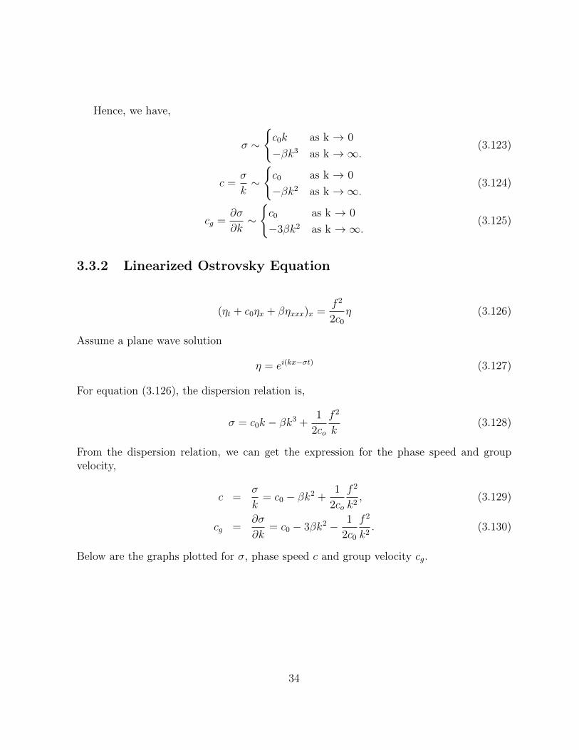
η (3.126)

Assume a plane wave solution

η = ei(kx−σt) (3.127)

For equation (3.126), the dispersion relation is,

σ = c0k − βk3 +1

2co

f 2

k(3.128)

From the dispersion relation, we can get the expression for the phase speed and groupvelocity,

c =σ

k= c0 − βk2 +

1

2co

f 2

k2, (3.129)

cg =∂σ

∂k= c0 − 3βk2 − 1

2c0

f 2

k2. (3.130)

Below are the graphs plotted for σ, phase speed c and group velocity cg.

34

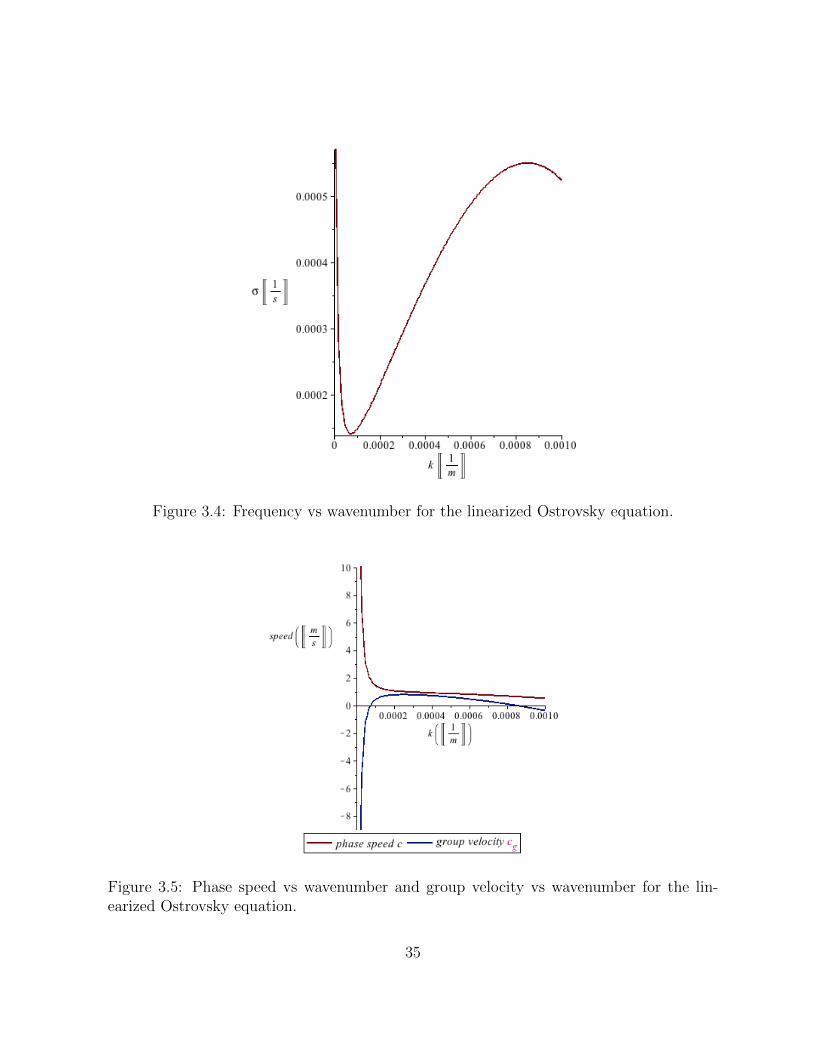
Figure 3.4: Frequency vs wavenumber for the linearized Ostrovsky equation.

Figure 3.5: Phase speed vs wavenumber and group velocity vs wavenumber for the lin-earized Ostrovsky equation.

35

Hence, we have,

σ ∼

1

2c0

f2

kas k → 0

−βk3 as k →∞.(3.131)

c =σ

k∼

1

2c0

f2

k2as k → 0

−βk2 as k →∞.(3.132)

cg =∂σ

∂k∼

− 1

2c0

f2

k2as k → 0

−3βk2 as k →∞.(3.133)

3.3.3 Linearized Alternative form of Ostrovsky Equation

(ηt + c0ηx + βηxxx)t = −f2

2η (3.134)

Assume a plane wave solution

η = ei(kx−σt) (3.135)

For equation (3.134), the dispersion relation is,

σ2 − (c0k − βk3)σ − f 2

2= 0 (3.136)

This is a quadratic equation, so we have two values for the frequencies.

σ1 =(c0k − βk3) +

√(c0k − βk3)2 + 2f 2

2(3.137)

σ2 =(c0k − βk3)−

√(c0k − βk3)2 + 2f 2

2(3.138)

Below are the graphs plotted for σ1 and σ2, the corresponding phase speeds and groupvelocities.

36

Figure 3.6: Frequency σ1 vs wavenumber for the linearized alternative form of Ostrovskyequation.

Figure 3.7: Phase speed c1 vs wavenumber and group velocity cg1 vs wavenumber for thelinearized alternative form of Ostrovsky equation.

37

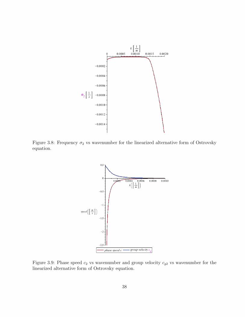
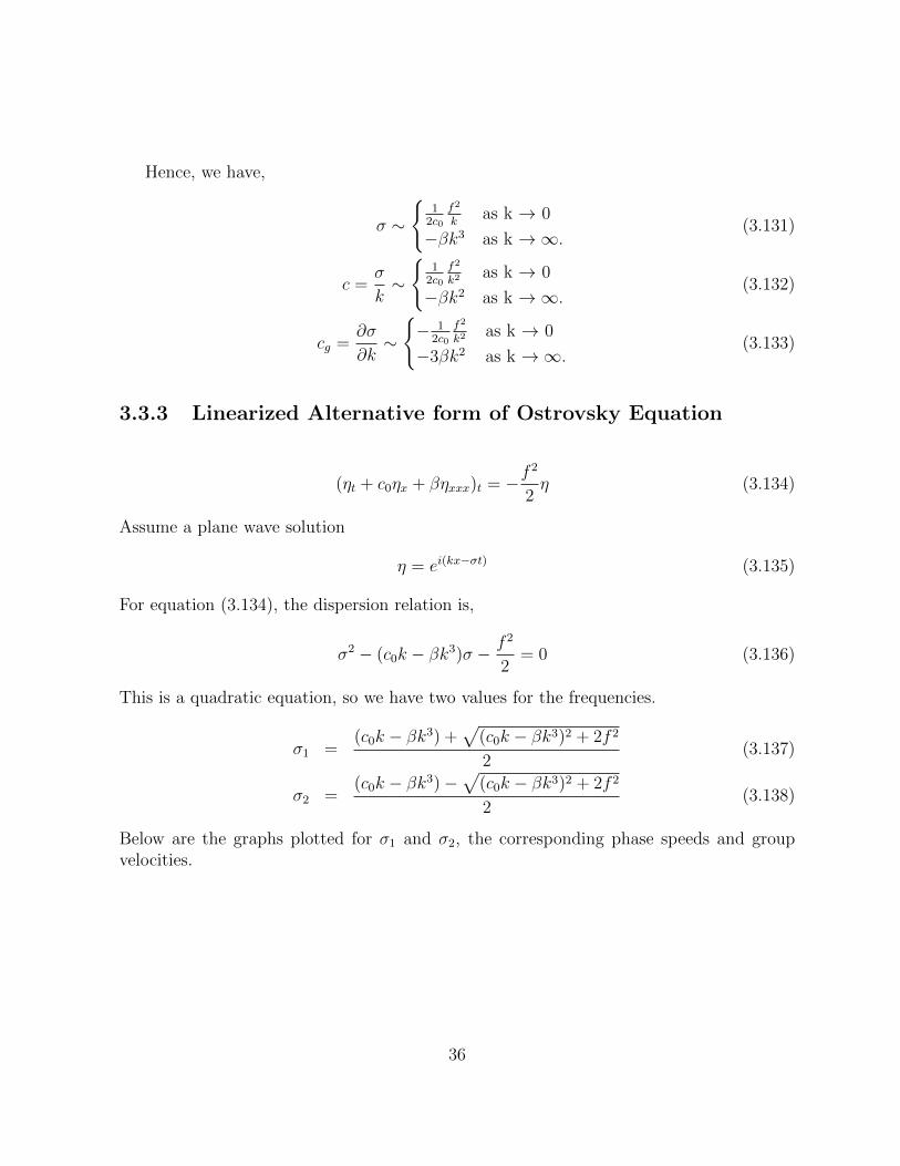
Figure 3.8: Frequency σ2 vs wavenumber for the linearized alternative form of Ostrovskyequation.

Figure 3.9: Phase speed c2 vs wavenumber and group velocity cg2 vs wavenumber for thelinearized alternative form of Ostrovsky equation.

38

Hence, we have,

σ1 ∼

f√2

as k → 0f2

2βk3as k →∞.

(3.139)

c1 =σ

k∼

f√2k

as k → 0f2

2βk4as k →∞.

(3.140)

cg1 =∂σ

∂k∼

c0(1

2+ 1

2√

2f) as k → 0

−32f2

βk4as k →∞.

(3.141)

σ2 ∼

− f√

2as k → 0

−βk3 as k →∞.(3.142)

c2 =σ

k∼

− f√

2kas k → 0

−βk2 as k →∞.(3.143)

cg2 =∂σ

∂k∼

12c0 as k → 0

−3βk2 as k →∞.(3.144)

3.3.4 Comparisons

The graphs of the four frequencies, group velocities and phase speeds are shown below,where the plots of the fully linear equations (2.29) to (2.33), the linearized KdV equation(3.118), the linearized Ostrovsky equation (3.126) and the linearized alternative Ostrovskyequation (3.134) are represented by the red, yellow, black and the blue lines, respectively.Since we are only interested in the rightward propagating wave, the negative frequency inthe linearized alternative Ostrovsky equation is not considered here.

39

Figure 3.10: Frequency vs wavenumber.

Figure 3.11: Phase speed vs wavenumber.

40

Figure 3.12: Group velocity vs wavenumber.

When k goes to 0, the frequencies for the fully linear equations (2.29) to (2.33) andfor the linearized alternative Ostrovsky (3.134) go to constant values f and f√

2separately,

while both of the phase speeds are inversely proportional to k. Compared with the otherthree equations, the linearized KdV equation does not capture the behavior of the fre-quency and the phase speed very well, because of the absence of the Coriolis term in theequation. The linearized Ostrovsky equation fails to describe the behavior of the groupvelocity by giving it negative values when k approaches 0. Hence, compared with theresult from the linearized momentum equations (2.29) to (2.33), the linearized alternativeOstrovsky equation seems to be the best of all the weakly nonlinear models.However, when k is very small, i.e. k < 0.0001 m−1 in these plots, the weakly nonlinearequations do not perform very well. This is probably because that, rotational effect dom-inates when the wavelength becomes very long. Meanwhile, all of the weakly nonlinearmodels assume the rotation to be O(ε) in its derivation, which is not appropriate for verylong waves. As a result, there is an intermediate valid range for the weakly nonlinearequations, i.e., around 0.0001 m−1 < k < 0.0007 m−1 in this case.When k goes to∞, none of the weakly-nonlinear equations (3.118), (3.126), (3.134) predictσ, c and cg very well, since these equations are only valid for long waves.We would expect the weakly nonlinear equations to be valid when the wave is suffientlylong, which means the wavelength is much larger than the water depth. However, thewavelength cannot be too long, since the rotational effects are assumed to be small.

In this chapter, a new equation called the alternative Ostrovsky equation is presentedas well as a short derivation of the Ostrovsky equation. Soliton solutions to the KdV andthe Gardner equation are given. The frequencies, phase speeds and group velocities of

41

all the linearized equations are discussed. From the analysis of the linearized equations,the weakly nonlinear models are expected to perform well only within a certain range ofwavenumber k.

42

Chapter 4

Numerical Model Setup

4.1 Fully Nonlinear Model: IGW

The equations used here are the incompressible Euler equations on an f-plane

D~U

Dt+ 2~Ω× ~U = −

~∇pρ0

− ρ

ρ0

gk, (4.1)

~∇ · ~U = 0, (4.2)

Dρ

Dt= 0, (4.3)

which are derived in Chapter 2. Here 2~Ω × ~U = (−fv, fu, 0), i.e., f-plane. Rigid lidapproximation is imposed on the water surface. The model was introduced by Lamb in1994 ([34]) and ([35]), but the method is due to Bell, Collela and Glaz and Bell and Marcus.

4.1.1 Solitary Wave Initialization

The initial condition is a single solitary wave solution of the DJL equation derived insection 2.3:

∇2ζ +N2(z − ζ)

c2ζ = 0. (4.4)

The boundary conditions are

ζ = 0 at z = 0, H (4.5)

ζ = 0 as x = ±L, (4.6)

43

where L is large. There are different techniques to solve the DJL equation. The IGW codeuses a variational technique to minimize the kinetic energy for the functional ([5])

F (ζ) =1

H

∫∫R

∫ ζ(x,z)

0

(ρ(z − ζ(x, z))− ρ(z − s)

)ds dx dz, (4.7)

where R is the computational subdomain in which the initial wave is computed. Theavailable potential energy of the wave in an infinitely long domain is equal to gHF (ζ),which determines the amplitude of the solitary wave. Only mode-one solitary waves canbe computed since the derivation of the DJL equation assumes a wave of permanent formand higher-mode solitary-like waves are generally accompanied by lower-mode, dispersivewaves which creates energy loss from the leading wave and hence it is not steady ([62]).More details of solving the DJL equation can be found in ([35]).

4.1.2 Stratification, Topography and Boundary Conditions

The stratification considered in this model is

ρ(z) = ρ1 + s1z + s2F (z,−Zpyc1, dpyc1) + s3F (z,−Zpyc2, dpyc2) (4.8)

Here ρ1 is the density at the surface; ρ1, s1, s2 and s3 are constants; F is a function thatgoes from a line with slope 0 to a line with slope 2. The transition occurs at Zpyc1 andZpyc2. dpyc1 and dpyc2 determine the thickness of the transition region. There is only onepycnocline in this stratification. F (x, Z, d) is defined as,

F (x, Z, d) = (x− Z) + d(log(cosh(x− Zd

)) + log 2). (4.9)

To have a clearer understanding of the stratification profile, we can re-write F (x, Z, d) as

F (x, Z, d) =

∫ x

Z

(1 + tanh(

x′ − Zd

))dx′. (4.10)

We want the change of the density, i.e. F ′, to be constant at first, then slowly increases withdepth, and remain constant at some value. 1 + tanh(x

′−Zd

) is chosen to be F ′. tanh(x′−Zd

)allows us to pick the changing point and the thickness of this changing region. In addition,we can integrate it analytically.The water depth is 500 m deep and the bottom is flat. The stratification is plotted in(4.1).

44

Figure 4.1: water depth vs density

The model uses the inflow and outflow boundary conditions. The flow is assumed to behydrostatic at the right boundary. Waves pass through with little reflection however shorthydrostatic waves will reflect off the boundary. In practice the right boundary is placed farenough from the region of interest that reflected waves are not a problem. ut is specifiedat the left boundary.

4.1.3 Numerical Method

Projection Method

A second-order projection method is used to solve the model equations. The Helmholtzdecomposition says that any vector ~V can be decomposed into the sum of a divergence freevector and the multiple of a strictly positive scalar function a(x, z) and a gradient, i.e.,

~V = ~V D + a~∇φ, (4.11)

45

where a(x, z) is a known given function. Then we can define a projection operator Pa that

maps the vector ~V onto its divergence free part.

Pa(~V ) = ~V D (4.12)

Pa depends on both of the function a and the boundary conditions. Now we consider themomentum equation, which can be written as

~Ut +~∇pρ0

= −~U · ~∇~U − 2~Ω× ~U − ρ

ρ0

gk. (4.13)

The left hand side of the equation has a divergence free vector ~Ut and a positive scalartimes the gradient of the pressure term. Since the Boussinesq approximation has been

made so a(x, z) = 1 and ~∇φ =~∇pρ0

. Thus we can define a projection operator Pρ so that

~Ut = Pρ(−~U · ~∇~U − 2~Ω× ~U − ρ

ρ0

gk). (4.14)

Computational Grids

Terrain-following (σ) coordinates are used. The grid cells are created by mapping thephysical domain, with coordinates (x, z), to the computational domain, with coordinates(ξ, ζ), via the transformation

(ξ, ζ) = (ξ(x, z), ζ(x, z)). (4.15)

Thus, the computational grid is a quadrilateral grid with I cells in the horizontal andJ cells in the vertical. All the grid cells are unit squares and the grid points are evenlyspaced. As a result, the equations calculated in the code are treated as functions of ξ andζ.

4.2 Weakly Nonlinear Model

4.2.1 Alternative Ostrovsky equation solver

The model considered here is the integral form of the alternative Ostrovsky equation de-rived in Chapter 3. [a, b] is the domain.

ηt + c0ηx + εαηηx + µβηxxx + ε2α1η2ηx = −f

2

2

∫ t

0

ηdt′ +f 2

2c0

∫ x

a

η(x′, 0)dx′ (4.16)

46

Solitary Wave Initialization

Based on our discussion on section (3.1.4), the initial condition of the wave profile shallsatisfy ∫ b

a

η(x′, 0)dx′ = 0. (4.17)

Two different initial condition have been tested in order to fulfill the conservativeintegral. One initial condition is a combination of two internal waves with one solitarywave of depression and the other wave of elevation that is the same shape as the solitarywave. Each solitary wave is the solution of the eKdV equation.

Figure 4.2: Solitary wave of depression. This is the wave solution of the eKdV equation.

47

Figure 4.3: Wave initialization for the alternative Ostrovsky equation. The spikes showthe locations of the initial wave of elevation and depression.

However, this initial condition has caused some oscillations at the tail of the leading de-pression solitary wave. All the plots below show that, η is constant but oscillates betweenabout -3 m and +3 m behind the leading wave (to left of about -2e5 m ). This oscillation

is probably caused by the term f2

2c0

∫ xaη(x′, 0)dx′ on the right hand side of the alternative

Ostrovsky equation. This term is independent of time and if the wave of elevation is toonarrow and far away from the leading wave, obvious oscillation may be observed in thewave tail.

48

−15 −10 −5 0 5

x 105

−80

−70

−60

−50

−40

−30

−20

−10

0

10

x(m)

z(m

)

Figure 4.4: Time = 6000 s

−15 −10 −5 0 5

x 105

−80

−70

−60

−50

−40

−30

−20

−10

0

10

x(m)

z(m

)

Figure 4.5: Time = 12000 s

−15 −10 −5 0 5

x 105

−80

−70

−60

−50

−40

−30

−20

−10

0

10

x(m)

z(m

)

Figure 4.6: Time = 168000 s

−15 −10 −5 0 5

x 105

−80

−70

−60

−50

−40

−30

−20

−10

0

10

x(m)

z(m

)

Figure 4.7: Time = 240000 s

This implies that instead of a second narrow wave of elevation far behind the leadingwave, I should use a small long wave immediately behind the leading wave. Thus, the sec-ond initial condition is a combination of one depression solitary wave and a long elevationwave behind it.

49

−2 −1.5 −1 −0.5 0 0.5 1 1.5 2

x 106

−80

−70

−60

−50

−40

−30

−20

−10

0

10

x(m)

z(m

)

Figure 4.8: Initial wave profile

−10 −9 −8 −7 −6 −5 −4 −3 −2

x 105

−0.5

−0.4

−0.3

−0.2

−0.1

0

0.1

0.2

0.3

0.4

0.5

x(m)

z(m

)

Figure 4.9: Zoomed in view of the initialelevation

Here the wavelength of the elevation wave is around 1000 km. Different wavelengthshave been tested and plots are made below. Blue, green, red lines represent longer, currentchoice and shorter wavelengths.

−3 −2.5 −2 −1.5 −1 −0.5 0 0.5

x 106

−80

−70

−60

−50

−40

−30

−20

−10

0

10

x(m)

z(m

)

Figure 4.10: Time = 72000 s

−3 −2.5 −2 −1.5 −1 −0.5 0 0.5

x 106

−80

−70

−60

−50

−40

−30

−20

−10

0

10

x(m)

z(m

)

Figure 4.11: Time = 144000 s

50

−20 −15 −10 −5 0 5

x 105

−80

−70

−60

−50

−40

−30

−20

−10

0

10

x(m)

z(m

)

Figure 4.12: Time = 216000 s

−3 −2.5 −2 −1.5 −1 −0.5 0 0.5

x 106

−80

−70

−60

−50

−40

−30

−20

−10

0

10

x(m)

z(m

)

Figure 4.13: Time = 300000 s

It seems that as long as the wavelength is quite long, the difference in the wavlengthof the elevation wave does not affect the shapes of the leading wave and the followingsolitary-like wave. The wave tail behinds all of the solitary-like small waves is slightlyinfluenced. However, we are mostly interested in the leading wave profile and the changesof the following small waves. As a result, the current choice of the wavelength seemsappropriate.

Stratification, Topography and Boundary Condition

The stratification used for this equation is exactly the same as that in the fully nonlinearmodel, and the bottom is flat. The boundary conditions in this model are

η1 = η2 = ηI−1 = ηI = 0. (4.18)

Numerical Method

All the coefficients in the equation are constant, since the water depth does not change.Both of the time and the space grids are uniform. We apply the finite difference methodto our model equation. The trapezoidal rule is used for the integral.

ηj+1n − ηj−1

n

2dt= −c0

ηjn+1 − ηjn−1

2dx− αηjn

ηjn+1 − ηjn−1

2dx(4.19)

−α1(ηjn)2ηjn+1 − η

jn−1

2dx− β

ηjn+2 − 2ηjn+1 + 2ηjn−1 − ηjn−2

2dx3(4.20)

−f2

2· dt

2

j∑m=0

(ηmn + ηm+1n ) +

f 2

2c0

· dx2

n∑s=0

(η0s + η0

s+1) (4.21)

51

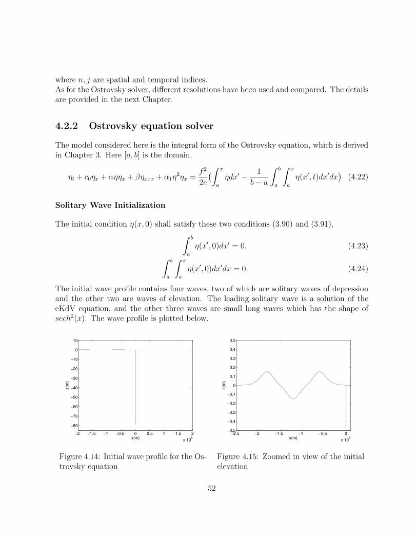
where n, j are spatial and temporal indices.As for the Ostrovsky solver, different resolutions have been used and compared. The detailsare provided in the next Chapter.

4.2.2 Ostrovsky equation solver

The model considered here is the integral form of the Ostrovsky equation, which is derivedin Chapter 3. Here [a, b] is the domain.

ηt + c0ηx + αηηx + βηxxx + α1η2ηx =

f 2

2c

(∫ x

a

ηdx′ − 1

b− a

∫ b

a

∫ x

a

η(x′, t)dx′dx)

(4.22)

Solitary Wave Initialization

The initial condition η(x, 0) shall satisfy these two conditions (3.90) and (3.91),∫ b

a

η(x′, 0)dx′ = 0, (4.23)∫ b

a

∫ x

a

η(x′, 0)dx′dx = 0. (4.24)

The initial wave profile contains four waves, two of which are solitary waves of depressionand the other two are waves of elevation. The leading solitary wave is a solution of theeKdV equation, and the other three waves are small long waves which has the shape ofsech2(x). The wave profile is plotted below.

−2 −1.5 −1 −0.5 0 0.5 1 1.5 2

x 106

−80

−70

−60

−50

−40

−30

−20

−10

0

10

x(m)

z(m

)

Figure 4.14: Initial wave profile for the Os-trovsky equation

−2.5 −2 −1.5 −1 −0.5 0

x 106

−0.5

−0.4

−0.3

−0.2

−0.1

0

0.1

0.2

0.3

0.4

0.5

x(m)

z(m

)

Figure 4.15: Zoomed in view of the initialelevation

52

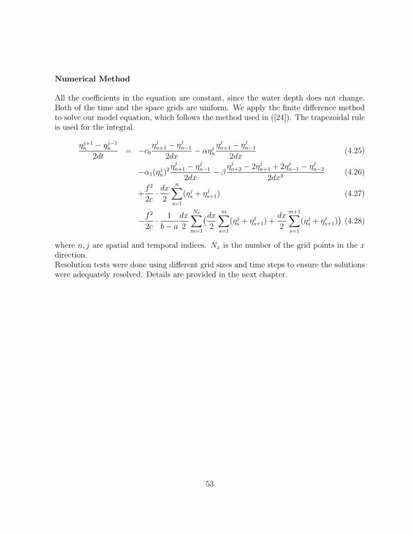
Numerical Method

All the coefficients in the equation are constant, since the water depth does not change.Both of the time and the space grids are uniform. We apply the finite difference methodto solve our model equation, which follows the method used in ([24]). The trapezoidal ruleis used for the integral.

ηj+1n − ηj−1

n

2dt= −c0

ηjn+1 − ηjn−1

2dx− αηjn

ηjn+1 − ηjn−1

2dx(4.25)

−α1(ηjn)2ηjn+1 − η

jn−1

2dx− β

ηjn+2 − 2ηjn+1 + 2ηjn−1 − ηjn−2

2dx3(4.26)

+f 2

2c· dx

2

n∑s=1

(ηjs + ηjs+1) (4.27)

−f2

2c· 1

b− adx

2

Nx∑m=1

(dx2

m∑s=1

(ηjs + ηjs+1) +dx

2

m+1∑s=1

(ηjs + ηjs+1))

(4.28)

where n, j are spatial and temporal indices. Nx is the number of the grid points in the xdirection.Resolution tests were done using different grid sizes and time steps to ensure the solutionswere adequately resolved. Details are provided in the next chapter.

53

Chapter 5

Simulation Results

5.1 Resolution Test

All of the model tests use initial waves of amplitudes = 79 m. Smaller waves are not tested.The water depth is set to be 500 m.

5.1.1 IGW model

One set of simulations has been run to find the appropriate dx and dt. The first set includesone case using a low resolution, i.e., dx=20 m and dt=2.5 s. The high resolution uses dt =1.5 s and dx = 20 m. The plot at time = 0 s is omitted. Figure (5.1) compares the waveprofile from the low and the high resolution. The plot on the left is a general look of thewhole wave profile, and the plot on the right is zoomed in for the amplitudes.

54

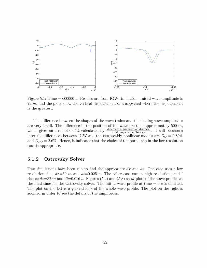
−2 −1.8 −1.6 −1.4 −1.2 −1

x 105

−80

−70

−60

−50

−40

−30

−20

−10

0

10

x(m)

z(m

)

high resolution

low resolution

−1.15 −1.1 −1.05

x 105

−40

−35

−30

−25

−20

−15

−10

−5

0

5

10

x(m)

z(m

)

high resolution

low resolution

Figure 5.1: Time = 600000 s. Results are from IGW simulation. Initial wave amplitude is79 m, and the plots show the vertical displacement of a isopycnal where the displacementis the greatest.

The difference between the shapes of the wave trains and the leading wave amplitudesare very small. The difference in the position of the wave crests is approximately 500 m,which gives an error of 0.04% calculated by |difference of propagation distance|

total propagation distance. It will be shown

later the differences between IGW and the two weakly nonlinear models are DO = 0.89%and DAO = 2.6%. Hence, it indicates that the choice of temporal step in the low resolutioncase is appropriate.

5.1.2 Ostrovsky Solver

Two simulations have been run to find the appropriate dx and dt. One case uses a lowresolution, i.e., dx=50 m and dt=0.025 s. The other case uses a high resolution, and Ichoose dx=32 m and dt=0.016 s. Figures (5.2) and (5.3) show plots of the wave profiles atthe final time for the Ostrovsky solver. The initial wave profile at time = 0 s is omitted.The plot on the left is a general look of the whole wave profile. The plot on the right iszoomed in order to see the details of the amplitudes.

55

−14 −12 −10 −8 −6 −4 −2

x 104

−80

−70

−60

−50

−40

−30

−20

−10

0

10

x(m)

z(m

)

high resolution

low resolution

−2.1 −2 −1.9 −1.8 −1.7 −1.6 −1.5 −1.4

x 104

−80

−70

−60

−50

−40

−30

−20

−10

0

10

x(m)

z(m

)

high resolution

low resolution

Figure 5.2: Time = 300000 s for the Ostrovsky solver. Plots show the vertical displacementof the isopycnal.

−1.8 −1.7 −1.6 −1.5 −1.4 −1.3 −1.2 −1.1 −1 −0.9 −0.8 −0.7

x 105

−80

−70

−60

−50

−40

−30

−20

−10

0

10

x(m)

z(m

)

high resolution

low resolution

−10 −9.8 −9.6 −9.4 −9.2 −9 −8.8 −8.6 −8.4 −8.2 −8

x 104

−40

−35

−30

−25

−20

−15

−10

−5

0

5

10

x(m)

z(m

)

high resolution

low resolution

Figure 5.3: Time = 600000 s for the Ostrovsky solver. Plots show the vertical displacementof the isopycnal.

From the plots we can see that the shape of the wave train is almost the same. Theamplitude difference is very small as well. The difference between the two wave crests arearound 2750 m and the total propagation distance is around 1.4e6 m. The difference isabout 0.20%, which is very small. This shows that the choice of spatial and time steps inthe low resolution are appropriate.

56

5.1.3 Alternative Ostrovsky Solver

All the choices of the spatial and the time steps are the same as that in the Ostrovskysolver. Details are omitted here. Below are some plots of the wave profiles at differenttime steps for the alternative Ostrovsky solver. The plot on the left is a general look ofthe whole wave profile. The plots on the right are zoomed in for the amplitudes.

−12 −10 −8 −6 −4 −2 0

x 104

−80

−70

−60

−50

−40

−30

−20

−10

0

10

x(m)

z(m

)

high resolution

low resolution

−1.6 −1.5 −1.4 −1.3 −1.2 −1.1 −1

x 104

−80

−70

−60

−50

−40

−30

−20

−10

0

10

x(m)

z(m

)

high resolution

low resolution

Figure 5.4: Time = 300000 s for the alternative Ostrovsky solver.

−1.8 −1.6 −1.4 −1.2 −1 −0.8 −0.6

x 105

−80

−70

−60

−50

−40

−30

−20

−10

0

10

x(m)

z(m

)

high resolution

low resolution

−8 −7.5 −7 −6.5

x 104

−40

−35

−30

−25

−20

−15

−10

−5

0

5

10

x(m)

z(m

)

high resolution

low resolution

Figure 5.5: Time = 600000 s for the alternative Ostrovsky solver.

From the plots we can see that the shape of the wave train is almost the same. Theamplitude difference is very small as well. The difference between the two wave crests arearound 2500 m and the total propagation distance is around 1.4e6 m. The difference isabout 0.18%, which is very small. This shows that the choice of spatial and time steps inthe low resolution are appropriate.

57

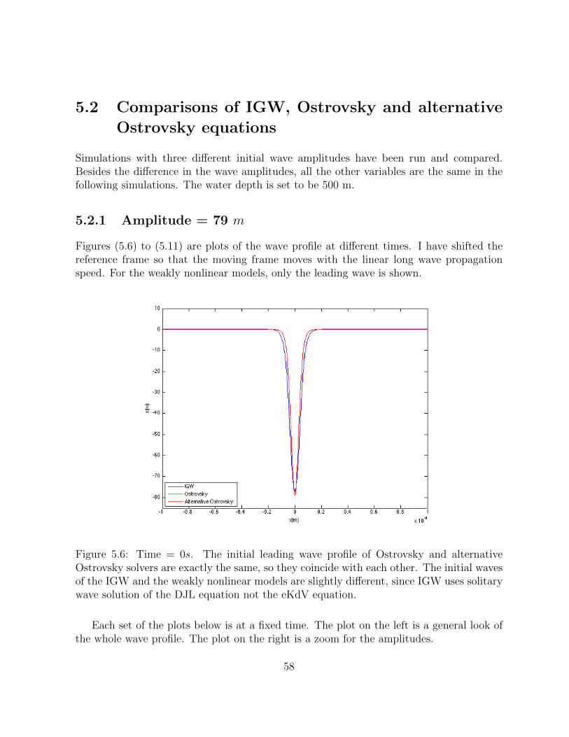
5.2 Comparisons of IGW, Ostrovsky and alternative

Ostrovsky equations

Simulations with three different initial wave amplitudes have been run and compared.Besides the difference in the wave amplitudes, all the other variables are the same in thefollowing simulations. The water depth is set to be 500 m.

5.2.1 Amplitude = 79 m

Figures (5.6) to (5.11) are plots of the wave profile at different times. I have shifted thereference frame so that the moving frame moves with the linear long wave propagationspeed. For the weakly nonlinear models, only the leading wave is shown.

Figure 5.6: Time = 0s. The initial leading wave profile of Ostrovsky and alternativeOstrovsky solvers are exactly the same, so they coincide with each other. The initial wavesof the IGW and the weakly nonlinear models are slightly different, since IGW uses solitarywave solution of the DJL equation not the eKdV equation.

Each set of the plots below is at a fixed time. The plot on the left is a general look ofthe whole wave profile. The plot on the right is a zoom for the amplitudes.

58

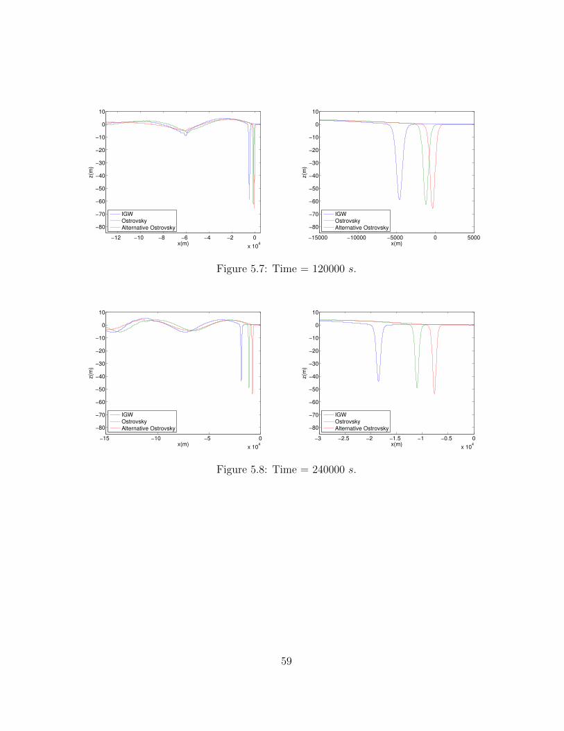
−12 −10 −8 −6 −4 −2 0

x 104

−80

−70

−60

−50

−40

−30

−20

−10

0

10

x(m)

z(m

)

IGW

Ostrovsky

Alternative Ostrovsky

−15000 −10000 −5000 0 5000

−80

−70

−60

−50

−40

−30

−20

−10

0

10

x(m)

z(m

)

IGW

Ostrovsky

Alternative Ostrovsky

Figure 5.7: Time = 120000 s.

−15 −10 −5 0

x 104

−80

−70

−60

−50

−40

−30

−20

−10

0

10

x(m)

z(m

)

IGW

Ostrovsky

Alternative Ostrovsky

−3 −2.5 −2 −1.5 −1 −0.5 0

x 104

−80

−70

−60

−50

−40

−30

−20

−10

0

10

x(m)

z(m

)

IGW

Ostrovsky

Alternative Ostrovsky

Figure 5.8: Time = 240000 s.

59

−14 −12 −10 −8 −6 −4 −2

x 104

−80

−70

−60

−50

−40

−30

−20

−10

0

10

x(m)

z(m

)

IGW

Ostrovsky

Alternative Ostrovsky

−5 −4.5 −4 −3.5 −3 −2.5 −2 −1.5 −1 −0.5

x 104

−80

−70

−60

−50

−40

−30

−20

−10

0

10

x(m)

z(m

)

IGW

Ostrovsky

Alternative Ostrovsky

Figure 5.9: Time = 300000 s.

−1.8 −1.6 −1.4 −1.2 −1 −0.8 −0.6 −0.4

x 105

−80

−70

−60

−50

−40

−30

−20

−10

0

10

x(m)

z(m

)

IGW

Ostrovsky

Alternative Ostrovsky−9 −8 −7 −6 −5 −4 −3

x 104

−40

−35

−30

−25

−20

−15

−10

−5

0

5

10

x(m)

z(m

)

IGW

Ostrovsky

Alternative Ostrovsky

Figure 5.10: Time = 480000 s.

60

−2 −1.8 −1.6 −1.4 −1.2 −1 −0.8

x 105

−80

−70

−60

−50

−40

−30

−20

−10

0

10

x(m)

z(m

)

IGW

Ostrovsky

Alternative Ostrovsky

−12 −11 −10 −9 −8 −7

x 104

−40

−35

−30

−25

−20

−15

−10

−5

0

5

10

x(m)

z(m

)

IGW

Ostrovsky

Alternative Ostrovsky

Figure 5.11: Time = 600000 s.

As time increases, all three models gives similar predictions of the shape of the wavetrain. At the final time, the wavenumber of the long wave trains predicted by each modelis kigw = 1.4e-4 m−1 (for IGW), kO = 1.3e-4 m−1 (for Ostrovsky) and kAO = 1.1e-4 m−1

(for Alternative Ostrovsky). The wavenumber keeps changing during the propagation. Forexample, at time t = 300000 s, kigw = 9.67e-5 m−1, kO = 8.98e-5 m−1 and kAO = 7.85e-5m−1. The wavenumber increases from t = 3e5 s to t = 6e5 s.The amplitudes predicted by the weakly nonlinear models are larger than that by theIGW. If we use the amplitude of the IGW as the standard, at the final time, the errors ofthe leading wave amplitudes from the two weakly nonlinear models are, AO = 20.7% andAAO = 65.5% larger, which are calculated as A =

|aweak−aigw|aigw

. The table below shows the

decaying process of the leading wave for each model.

Table 5.1: The amplitude decay of the leading wave

time for wavedecaying to 50%

time for wavedecaying to 25 %

at t = 6e5 s,(wave amplitudeinitial amplitude

)×

100%IGW 276000 s 504000 s 18 %Ostrovsky 324000 s 564000 s 22 %Alternative Ostrovsky 396000 s N/A 30 %

The weakly nonlinear models propagate faster than the IGW. At t = 600000 s, the errorsof propagation distances are, DO = 0.89% and DAO = 2.6% faster, which is calculated as

D =|dweak − dIGW |

total propagation distance. (5.1)

61

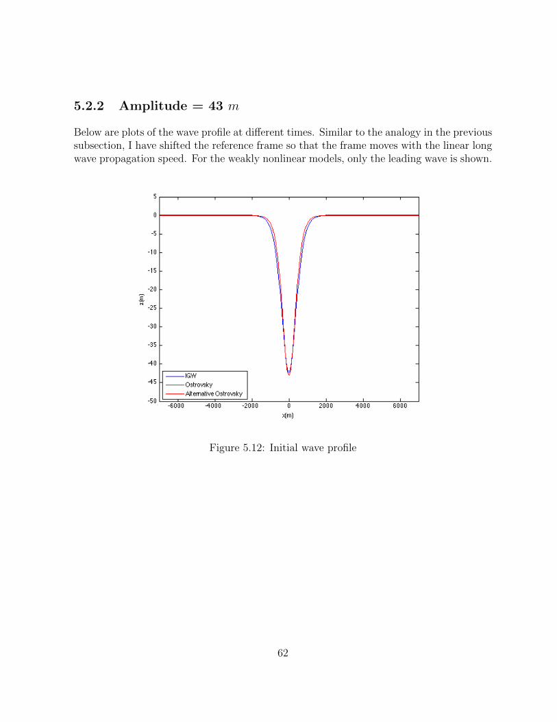
5.2.2 Amplitude = 43 m

Below are plots of the wave profile at different times. Similar to the analogy in the previoussubsection, I have shifted the reference frame so that the frame moves with the linear longwave propagation speed. For the weakly nonlinear models, only the leading wave is shown.

Figure 5.12: Initial wave profile

62

−12 −10 −8 −6 −4 −2 0

x 104

−50

−40

−30

−20

−10

0

10

x(m)

z(m

)

IGW

Ostrovsky

Alternative Ostrovsky

−15000 −10000 −5000 0 5000−50

−40

−30

−20

−10

0

10

x(m)

z(m

)

IGW

Ostrovsky

Alternative Ostrovsky

Figure 5.13: Time = 120000 s.

−10 −8 −6 −4 −2

x 104

−50

−40

−30

−20

−10

0

10

x(m)

z(m

)

IGW

Ostrovsky

Alternative Ostrovsky

−3 −2.5 −2 −1.5 −1 −0.5

x 104

−50

−40

−30

−20

−10

0

10

x(m)

z(m

)

IGW

Ostrovsky

Alternative Ostrovsky

Figure 5.14: Time = 240000 s.

63

−12 −11 −10 −9 −8 −7 −6 −5 −4 −3 −2 −1

x 104

−50

−40

−30

−20

−10

0

10

x(m)

z(m

)

IGW

Ostrovsky

Alternative Ostrovsky

−4 −3.5 −3 −2.5 −2 −1.5 −1

x 104

−50

−40

−30

−20

−10

0

10

x(m)

z(m

)

IGW

Ostrovsky

Alternative Ostrovsky

Figure 5.15: Time = 300000 s.

−14 −12 −10 −8 −6 −4

x 104

−50

−40

−30

−20

−10

0

10

x(m)

z(m

)

IGW

Ostrovsky

Alternative Ostrovsky

−10 −9 −8 −7 −6 −5 −4

x 104

−20

−15

−10

−5

0

5

10

x(m)

z(m

)

IGW

Ostrovsky

Alternative Ostrovsky

Figure 5.16: Time = 480000 s.

64

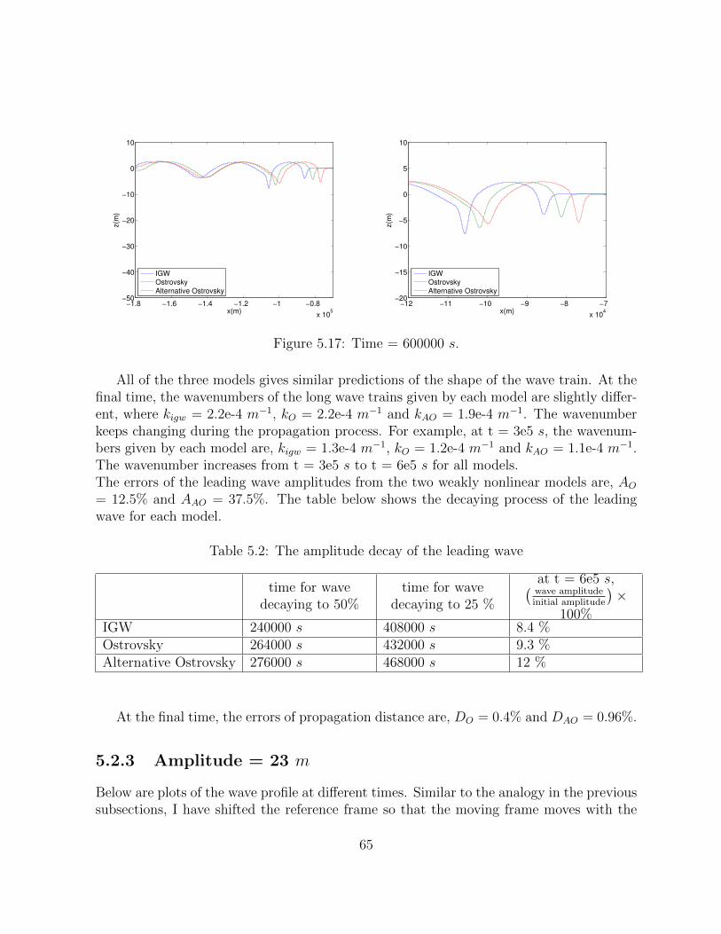
−1.8 −1.6 −1.4 −1.2 −1 −0.8

x 105

−50

−40

−30

−20

−10

0

10

x(m)

z(m

)

IGW

Ostrovsky

Alternative Ostrovsky

−12 −11 −10 −9 −8 −7

x 104

−20

−15

−10

−5

0

5

10

x(m)

z(m

)

IGW

Ostrovsky

Alternative Ostrovsky

Figure 5.17: Time = 600000 s.

All of the three models gives similar predictions of the shape of the wave train. At thefinal time, the wavenumbers of the long wave trains given by each model are slightly differ-ent, where kigw = 2.2e-4 m−1, kO = 2.2e-4 m−1 and kAO = 1.9e-4 m−1. The wavenumberkeeps changing during the propagation process. For example, at t = 3e5 s, the wavenum-bers given by each model are, kigw = 1.3e-4 m−1, kO = 1.2e-4 m−1 and kAO = 1.1e-4 m−1.The wavenumber increases from t = 3e5 s to t = 6e5 s for all models.The errors of the leading wave amplitudes from the two weakly nonlinear models are, AO= 12.5% and AAO = 37.5%. The table below shows the decaying process of the leadingwave for each model.

Table 5.2: The amplitude decay of the leading wave

time for wavedecaying to 50%

time for wavedecaying to 25 %

at t = 6e5 s,(wave amplitudeinitial amplitude

)×

100%IGW 240000 s 408000 s 8.4 %Ostrovsky 264000 s 432000 s 9.3 %Alternative Ostrovsky 276000 s 468000 s 12 %

At the final time, the errors of propagation distance are, DO = 0.4% and DAO = 0.96%.

5.2.3 Amplitude = 23 m

Below are plots of the wave profile at different times. Similar to the analogy in the previoussubsections, I have shifted the reference frame so that the moving frame moves with the

65

linear long wave propagation speed. For the weakly nonlinear models, only the leadingwave is shown.

−5000 0 5000−25

−20

−15

−10

−5

0

5

x(m)

z(m

)

IGW

Ostrovsky

Alternative Ostrovsky

Figure 5.18: Initial wave profile

−12 −10 −8 −6 −4 −2 0

x 104

−25

−20

−15

−10

−5

0

5

x(m)

z(m

)

IGW

Ostrovsky

Alternative Ostrovsky

−15000 −10000 −5000 0 5000−25

−20

−15

−10

−5

0

5

x(m)

z(m

)

IGW

Ostrovsky

Alternative Ostrovsky

Figure 5.19: Time = 120000 s.

66

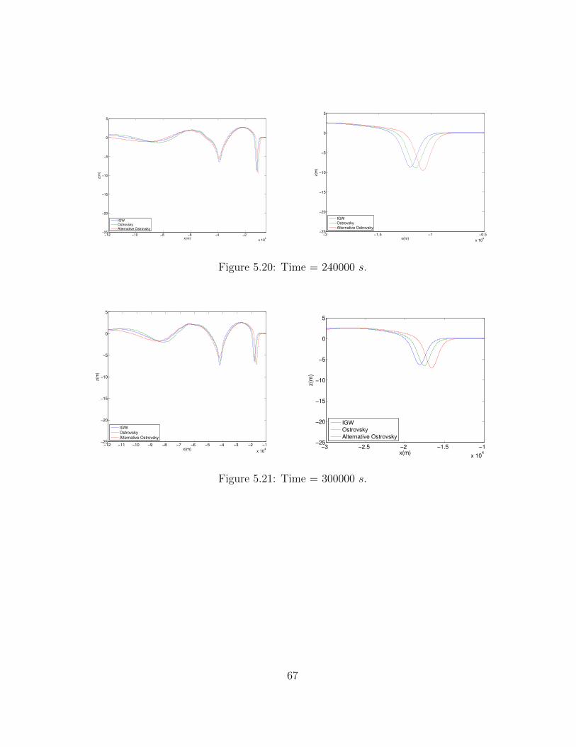
−12 −10 −8 −6 −4 −2

x 104

−25

−20

−15

−10

−5

0

5

x(m)

z(m

)

IGW

Ostrovsky

Alternative Ostrovsky

−2 −1.5 −1 −0.5

x 104

−25

−20

−15

−10

−5

0

5

x(m)

z(m

)

IGW

Ostrovsky

Alternative Ostrovsky

Figure 5.20: Time = 240000 s.

−12 −11 −10 −9 −8 −7 −6 −5 −4 −3 −2 −1

x 104

−25

−20

−15

−10

−5

0

5

x(m)

z(m

)

IGW

Ostrovsky

Alternative Ostrovsky

−3 −2.5 −2 −1.5 −1

x 104

−25

−20

−15

−10

−5

0

5

x(m)

z(m

)

IGW

Ostrovsky

Alternative Ostrovsky

Figure 5.21: Time = 300000 s.

67

−14 −12 −10 −8 −6 −4

x 104

−25

−20

−15

−10

−5

0

5

x(m)

z(m

)

IGW

Ostrovsky

Alternative Ostrovsky

−7 −6.5 −6 −5.5 −5 −4.5 −4 −3.5

x 104

−25

−20

−15

−10

−5

0

5

x(m)

z(m

)

IGW

Ostrovsky

Alternative Ostrovsky

Figure 5.22: Time = 480000 s.

−1.8 −1.6 −1.4 −1.2 −1 −0.8 −0.6

x 105

−25

−20

−15

−10

−5

0

5

x(m)

z(m

)

IGW

Ostrovsky

Alternative Ostrovsky

−8 −7.5 −7 −6.5 −6 −5.5 −5

x 104

−25

−20

−15

−10

−5

0

5

x(m)

z(m

)

IGW

Ostrovsky

Alternative Ostrovsky

Figure 5.23: Time = 600000 s.

All of the three models gives similar predictions of the shape of the wave train. At thefinal time, the wavenumber is difficult to measure and the leading wave is hardly observablefrom the plots. Instead, the second solitary-like wave is very clearly formed. The tablebelow shows the decaying process of the leading wave for each model.

68

Table 5.3: The amplitude decay of the leading wavetime for wavedecaying to

50%

time for wavedecaying to

25 %

time for wavedecaying to

10 %

at t = 6e5 s,(wave amplitudeinitial amplitude

)×

100%IGW 180000 s 312000 s 432000 s 2.6 %Ostrovsky 180000 s 324000 s 456000 s 2.6 %Alternative Ostrovsky 192000 s 336000 s 468000 s 3.4 %

From these three different simulation results, we can see that both of the weakly non-linear models manage to capture the changing behavior of the ISW while propagatingwith Earth’ rotation. The addition of the rotation term breaks the balance between thenonlinear effects and the dispersive effect. The energy is slowly diverted from the leadingwave to the wave train behind it. The nonlinear effects help the wave tail of the leadingwave to steepen up, thus form a smaller solitary-like wave behind it. Then the secondsolitary-like wave is formed in a similar way, followed by the first solitary-like wave. Thesedifferent solitary-like waves have different wavelengths, and they all propagate in differentspeeds due to the dispersive effects. If we take the results from IGW as the reference, theleading wave amplitudes and the propagation speeds predicted by the Ostrovsky solvermatch better with the IGW than that from the alternative Ostrovsky solver. Hence, theOstrovsky equation seems to give a better performance.

Comparing the results from the three sets of simulation, we can see that, as the ampli-tude of the initial wave decreases, the differences among the three models decreases andthe weakly nonlinear models become more accurate. This is reasonable since the weaklynonlinear models are derived based on the assumption that the wave amplitude is verysmall.

5.3 Simulation Analysis

The three models have predicted different wavelengths of the long wave tails, amplitudesand propagation speed of the leading waves. To analyze these different results, plots offrequencies, phase speeds and group velocities have been made from the linearized ver-sion of these three models. All the coefficients used in the plots are obtained from thecorresponding numerical simulations.

69

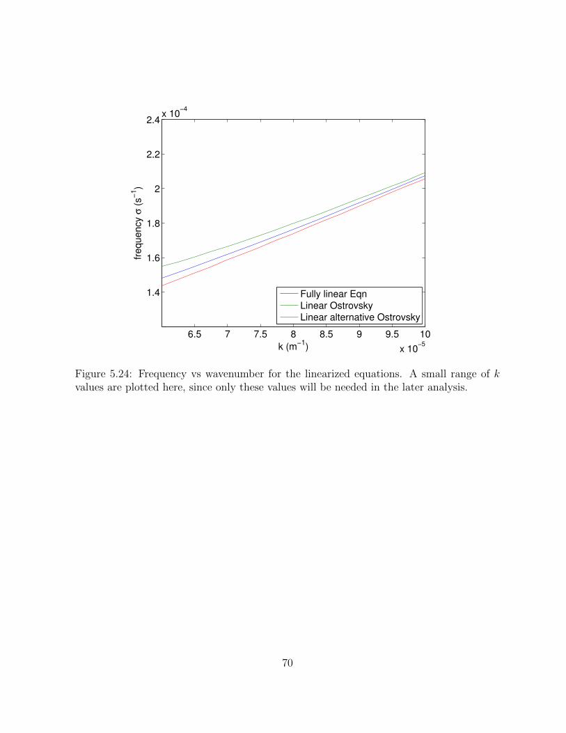
6.5 7 7.5 8 8.5 9 9.5 10

x 10−5

1.4

1.6

1.8

2

2.2

2.4x 10

−4

k (m−1

)

frequency σ

(s

−1)

Fully linear Eqn

Linear Ostrovsky

Linear alternative Ostrovsky

Figure 5.24: Frequency vs wavenumber for the linearized equations. A small range of kvalues are plotted here, since only these values will be needed in the later analysis.

70

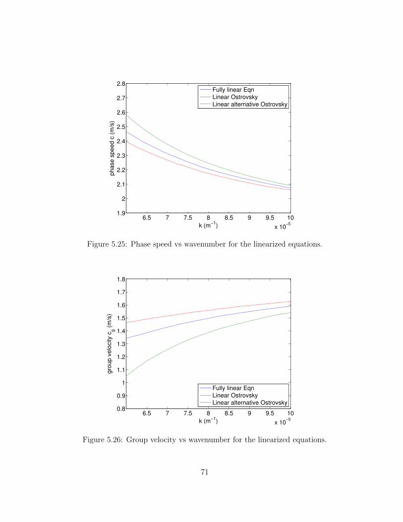
6.5 7 7.5 8 8.5 9 9.5 10

x 10−5

1.9

2

2.1

2.2

2.3

2.4

2.5

2.6

2.7

2.8

k (m−1

)

ph

ase

sp

ee

d c

(m

/s)

Fully linear Eqn

Linear Ostrovsky

Linear alternative Ostrovsky

Figure 5.25: Phase speed vs wavenumber for the linearized equations.

6.5 7 7.5 8 8.5 9 9.5 10

x 10−5

0.8

0.9

1

1.1

1.2

1.3

1.4

1.5

1.6

1.7

1.8

k (m−1

)

gro

up

ve

locity c

g (

m/s

)

Fully linear Eqn

Linear Ostrovsky

Linear alternative Ostrovsky

Figure 5.26: Group velocity vs wavenumber for the linearized equations.

71

When the amplitude of the initial wave is 79 m and at t = 300000 s, the wavenumbersof the long wave trains for each model are kigw = 9.67e-5 m−1, kO = 8.98e-5 m−1 and kAO= 7.85e-5 m−1, which we can get from the previous section. From the plots made above,we can see that the phase speeds of the three models are very close. The phase speed of thelinearized alternative Ostrovsky (LAO) equation is the fastest, then followed by linearizedOstrovsky (LO) and fully linear (LF) equations, which matches the simulation results.

Combining the plots of phase speeds and the plots of group velocities, we can get thevelocity of the wave train relative to the leading wave propagation speed. We name thisvelocity of the wave train as ∆c, which is calculated by ∆c = |c − cg|. The larger ∆c is,the more rapidly the energy is drained from the leading wave. Since this will decrease theamplitude of the leading wave, and decrease the wave propagation speed, the larger the∆c is, the slower the wave propagates. As such, we would expect ∆cLAO < ∆cLO < ∆cLF ,since cLAO > cLO > cLF . However, the data we get from the plots of the linearized equa-tions do not support this result.The two other cases with amplitudes = 43 m and 23 m give the similar results. The plotsare omitted here, and all the data is listed below.

Table 5.4: amplitude = 79mLF LO LAO

phase speed c (m/s) 2.09 2.15 2.19group velocity cg (m/s) 1.58 1.49 1.55∆c (m/s) 0.51 0.66 0.64

Table 5.5: amplitude = 43mLF LO LAO

phase speed c (m/s) 1.97 2.01 2.02group velocity cg (m/s) 1.68 1.63 1.65∆c (m/s) 0.29 0.38 0.37

Table 5.6: amplitude = 23mLF LO LAO

phase speed c (m/s) 1.891 1.893 1.898group velocity cg (m/s) 1.745 1.739 1.741∆c (m/s) 0.146 0.154 0.157

72

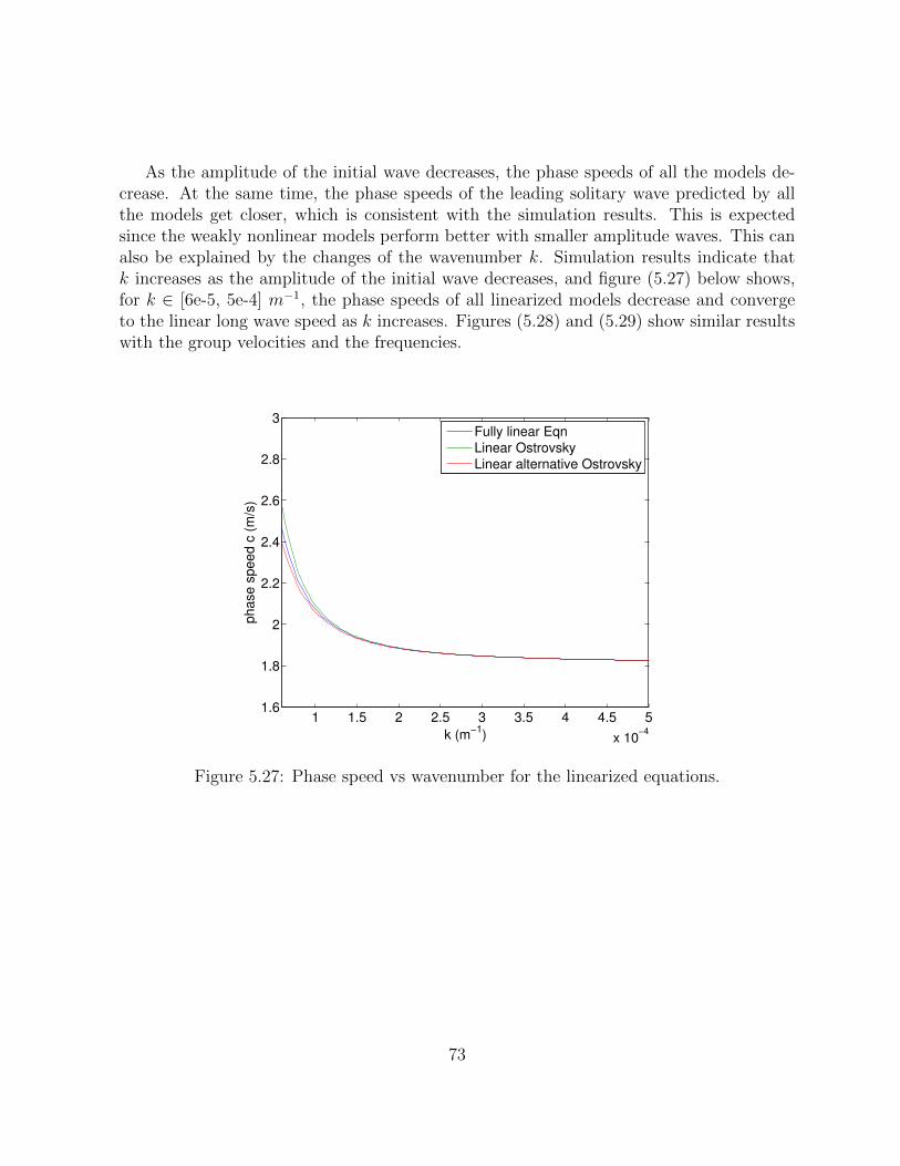
As the amplitude of the initial wave decreases, the phase speeds of all the models de-crease. At the same time, the phase speeds of the leading solitary wave predicted by allthe models get closer, which is consistent with the simulation results. This is expectedsince the weakly nonlinear models perform better with smaller amplitude waves. This canalso be explained by the changes of the wavenumber k. Simulation results indicate thatk increases as the amplitude of the initial wave decreases, and figure (5.27) below shows,for k ∈ [6e-5, 5e-4] m−1, the phase speeds of all linearized models decrease and convergeto the linear long wave speed as k increases. Figures (5.28) and (5.29) show similar resultswith the group velocities and the frequencies.

1 1.5 2 2.5 3 3.5 4 4.5 5

x 10−4

1.6

1.8

2

2.2

2.4

2.6

2.8

3

k (m−1

)

ph

ase

sp

ee

d c

(m

/s)

Fully linear Eqn

Linear Ostrovsky

Linear alternative Ostrovsky

Figure 5.27: Phase speed vs wavenumber for the linearized equations.

73

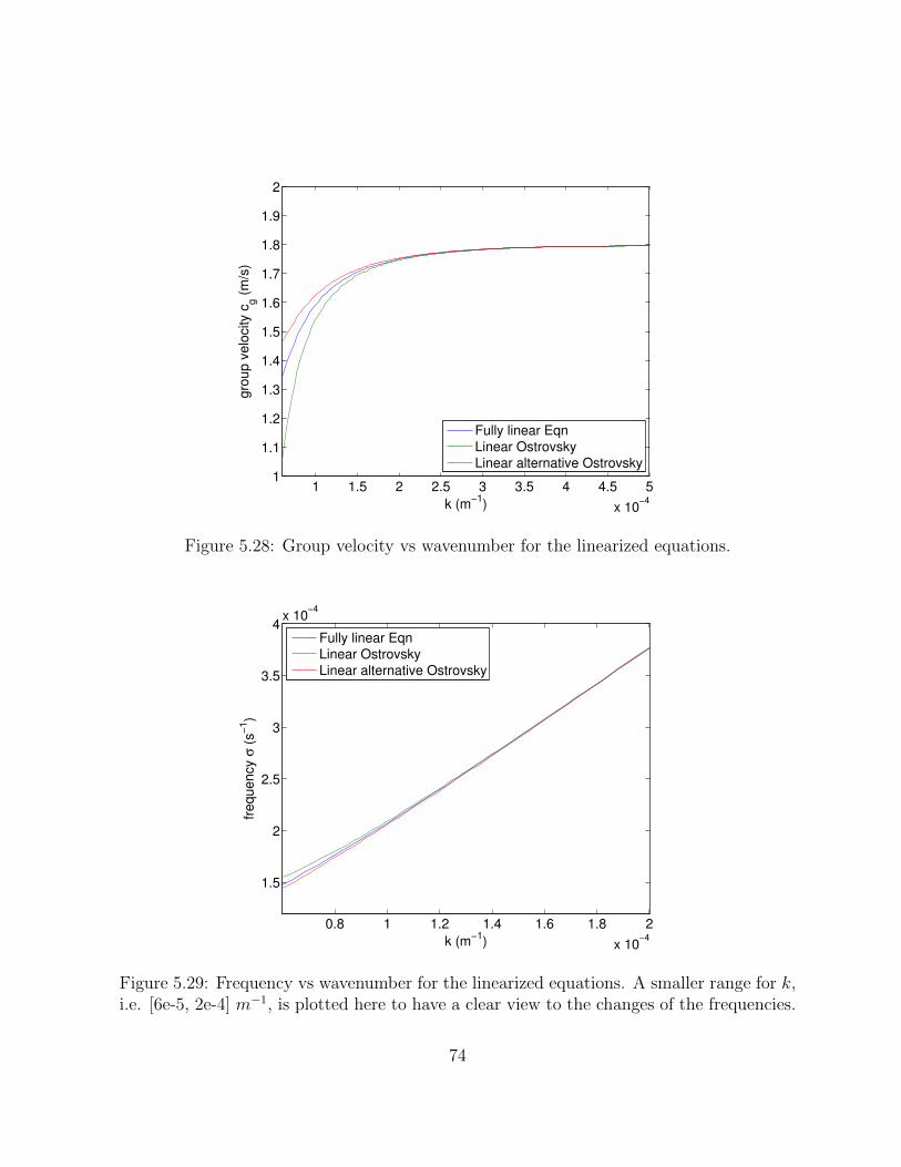
1 1.5 2 2.5 3 3.5 4 4.5 5

x 10−4

1

1.1

1.2

1.3

1.4

1.5

1.6

1.7

1.8

1.9

2

k (m−1

)

gro

up

ve

locity c

g (

m/s

)

Fully linear Eqn

Linear Ostrovsky

Linear alternative Ostrovsky

Figure 5.28: Group velocity vs wavenumber for the linearized equations.

0.8 1 1.2 1.4 1.6 1.8 2

x 10−4

1.5

2

2.5

3

3.5

4x 10

−4

k (m−1

)

fre

qu

en

cy σ

(s

−1)

Fully linear Eqn

Linear Ostrovsky

Linear alternative Ostrovsky

Figure 5.29: Frequency vs wavenumber for the linearized equations. A smaller range for k,i.e. [6e-5, 2e-4] m−1, is plotted here to have a clear view to the changes of the frequencies.

74

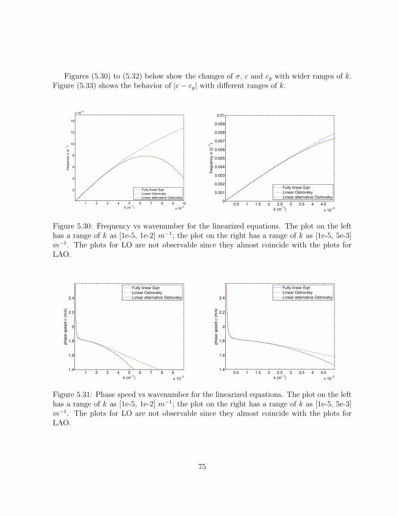
Figures (5.30) to (5.32) below show the changes of σ, c and cg with wider ranges of k.Figure (5.33) shows the behavior of |c− cg| with different ranges of k.

1 2 3 4 5 6 7 8 9 10

x 10−3

2

4

6

8

10

12

14

x 10−3

k (m−1

)

frequency σ

(s

−1)

Fully linear Eqn

Linear Ostrovsky

Linear alternative Ostrovsky

0.5 1 1.5 2 2.5 3 3.5 4 4.5

x 10−3

0

0.001

0.002

0.003

0.004

0.005

0.006

0.007

0.008

0.009

0.01

k (m−1

)fr

equency σ

(s

−1)

Fully linear Eqn

Linear Ostrovsky

Linear alternative Ostrovsky

Figure 5.30: Frequency vs wavenumber for the linearized equations. The plot on the lefthas a range of k as [1e-5, 1e-2] m−1; the plot on the right has a range of k as [1e-5, 5e-3]m−1. The plots for LO are not observable since they almost coincide with the plots forLAO.

1 2 3 4 5 6 7 8 9

x 10−3

1.4

1.6

1.8

2

2.2

2.4

k (m−1

)

phase s

peed c

(m

/s)

Fully linear Eqn

Linear Ostrovsky

Linear alternative Ostrovsky

0.5 1 1.5 2 2.5 3 3.5 4 4.5

x 10−3

1.4

1.6

1.8

2

2.2

2.4

k (m−1

)

phase s

peed c

(m

/s)

Fully linear Eqn

Linear Ostrovsky

Linear alternative Ostrovsky

Figure 5.31: Phase speed vs wavenumber for the linearized equations. The plot on the lefthas a range of k as [1e-5, 1e-2] m−1; the plot on the right has a range of k as [1e-5, 5e-3]m−1. The plots for LO are not observable since they almost coincide with the plots forLAO.

75

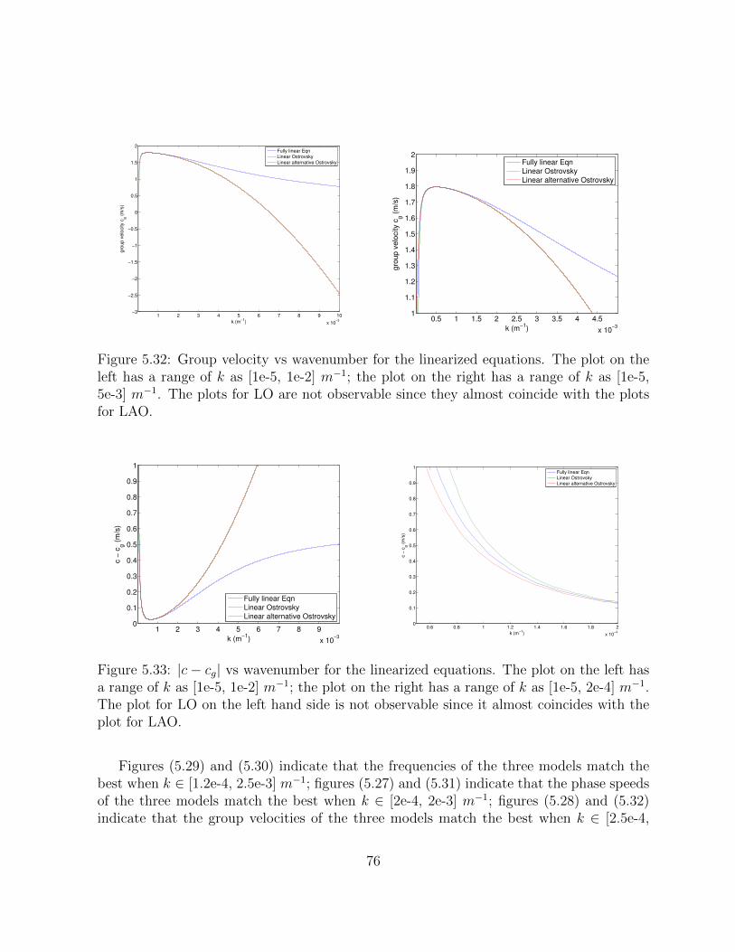
1 2 3 4 5 6 7 8 9 10

x 10−3

−3

−2.5

−2

−1.5

−1

−0.5

0

0.5

1

1.5

2

k (m−1

)

gro

up

ve

locity c

g (

m/s

)

Fully linear Eqn

Linear Ostrovsky

Linear alternative Ostrovsky

0.5 1 1.5 2 2.5 3 3.5 4 4.5

x 10−3

1

1.1

1.2

1.3

1.4

1.5

1.6

1.7

1.8

1.9

2

k (m−1

)

gro

up v

elo

city c

g (

m/s

)

Fully linear Eqn

Linear Ostrovsky

Linear alternative Ostrovsky

Figure 5.32: Group velocity vs wavenumber for the linearized equations. The plot on theleft has a range of k as [1e-5, 1e-2] m−1; the plot on the right has a range of k as [1e-5,5e-3] m−1. The plots for LO are not observable since they almost coincide with the plotsfor LAO.

1 2 3 4 5 6 7 8 9

x 10−3

0

0.1

0.2

0.3

0.4

0.5

0.6

0.7

0.8

0.9

1

k (m−1

)

c −

cg (

m/s

)

Fully linear Eqn

Linear Ostrovsky

Linear alternative Ostrovsky

0.6 0.8 1 1.2 1.4 1.6 1.8 2

x 10−4

0

0.1

0.2

0.3

0.4

0.5

0.6

0.7

0.8

0.9

1

k (m−1

)

c −

cg (

m/s

)

Fully linear Eqn

Linear Ostrovsky

Linear alternative Ostrovsky

Figure 5.33: |c− cg| vs wavenumber for the linearized equations. The plot on the left hasa range of k as [1e-5, 1e-2] m−1; the plot on the right has a range of k as [1e-5, 2e-4] m−1.The plot for LO on the left hand side is not observable since it almost coincides with theplot for LAO.

Figures (5.29) and (5.30) indicate that the frequencies of the three models match thebest when k ∈ [1.2e-4, 2.5e-3] m−1; figures (5.27) and (5.31) indicate that the phase speedsof the three models match the best when k ∈ [2e-4, 2e-3] m−1; figures (5.28) and (5.32)indicate that the group velocities of the three models match the best when k ∈ [2.5e-4,

76

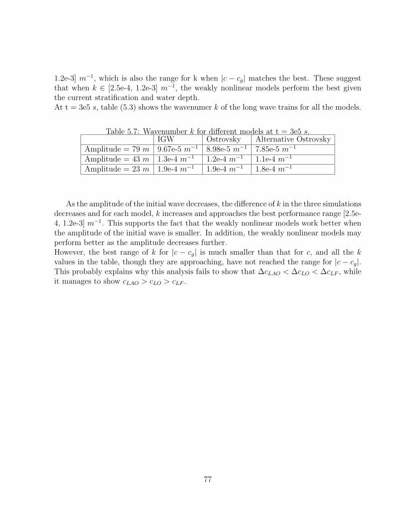
1.2e-3] m−1, which is also the range for k when |c − cg| matches the best. These suggestthat when k ∈ [2.5e-4, 1.2e-3] m−1, the weakly nonlinear models perform the best giventhe current stratification and water depth.At t = 3e5 s, table (5.3) shows the wavenumer k of the long wave trains for all the models.

Table 5.7: Wavenumber k for different models at t = 3e5 s.IGW Ostrovsky Alternative Ostrovsky

Amplitude = 79 m 9.67e-5 m−1 8.98e-5 m−1 7.85e-5 m−1

Amplitude = 43 m 1.3e-4 m−1 1.2e-4 m−1 1.1e-4 m−1

Amplitude = 23 m 1.9e-4 m−1 1.9e-4 m−1 1.8e-4 m−1

As the amplitude of the initial wave decreases, the difference of k in the three simulationsdecreases and for each model, k increases and approaches the best performance range [2.5e-4, 1.2e-3] m−1. This supports the fact that the weakly nonlinear models work better whenthe amplitude of the initial wave is smaller. In addition, the weakly nonlinear models mayperform better as the amplitude decreases further.However, the best range of k for |c − cg| is much smaller than that for c, and all the kvalues in the table, though they are approaching, have not reached the range for |c − cg|.This probably explains why this analysis fails to show that ∆cLAO < ∆cLO < ∆cLF , whileit manages to show cLAO > cLO > cLF .

77

Chapter 6

Conclusion

6.1 Summary

In this thesis, a new equation, alternative Ostrovsky equation, derived by Lamb ([33]),is introduced to model the behavior of ISWs with the Earth’s rotation. Following thederivation of the alternative Ostrovsky equation, the derivation of the Ostrovsky equa-tion has been briefly described. Two weakly nonlinear models, Ostrovsky and alternativeOstrovsky solvers, are used in the numerical simulations. Here the alternative Ostrovskysolver has been modified from the existing Ostrovsky solver. Finite difference method upto second-order accuracy is adopted in both of these two solvers. Solitary wave solutionsfrom Gardner equation are used as the initialization. Simulation results from the Ostrovskyand alternative Ostrovsky solvers are compared with the two-dimensional fully nonlinearmodel, i.e., IGW, to investigate the validity of the weakly nonlinear models. IGW uses so-lutions from DJL equation as the initial wave profile, and second-order projection methodis used as the numerical method.

In all of the numerical simulations, the water depth is set to 500 m and the bottom isflat. The stratification is an analytic expression given in (4.9). The thermocline lies be-tween water depth of 55 m and 120 m. We have run three sets of numerical simulationswith initial wave amplitudes of 79 m, 43 m and 23 m. The time span of each simulationis 600000 s, and the Coriolis parameter is taken as 10−4 rad/s, which is a typical value formid-latitudes. Resolution tests have been run for each model to determine the appropriatespatial and the temporal steps.

Based on the simulation results in the thesis, the Ostrovsky equation provides betterpredictions of the leading wave amplitudes and the propagation speeds than the alter-native Ostrovsky equation. As the initial wave amplitude decreases, the differences be-

78

tween the weakly nonlinear models also decrease. This agrees with the assumption of theweakly nonlinear models, i.e., ε ≈ a

H 1. In addition, as the initial wave amplitude

decreases, the wavenumber of each model increases and the wavelength decreases. Thisalso agrees with the assumption of the weakly nonlinear models that, µ = (H

L)2 1 and

δ = f2L2

c2= f2L2

N2H2 1, which suggests H2 L2 N2H2

f2. The weakly nonlinear models

perform well when the wavelength is long but not too long since the rotational effects areassumed to be small.

Analysis from the linearized equations further confirms this point. Given the currentwater depth and the stratification profile, a best performance range for the wavenumberof the long wave train is also suggested, which indicates that the weakly nonlinear modelsmay perform better if initial wave decreases further.

6.2 Future Work

The equations used in this thesis can be generalised to model different wave effects. Someextensions are listed below.

• Given the currect initial conditions in our simulations, the Ostrovsky equation per-forms better than the alternative Ostrovsky equation. However, the analysis from thelinearized equations suggests that the alternative Ostrovsky equation may performbetter when the wavelength of the wave is very long (≈ 160 km given the currentwater depth and the stratification profile). More simulations with different initialconditions, for example internal tides, may be considered.If the alternative Ostrovsky equation can perform better than the Ostrovsky equa-tion, we can probably consider to extend the alternative Ostrovsky equation to twodimensions. In this case, more waves can be modeled, for example Rossby waves,which needs β plane approximation.

• The water depth used in this thesis is 500 m. The ocean can go up to thousands ofmeters depth. We can increase the water depth to see the behavior of the deep waterwaves.

• We have only used one analytic stratification in our simulations. Other stratificationprofiles, including analytic and non-analytic, can be adopted.

• There are alternative equations equivalent to the weakly nonlinear equations up toO(ε2, µ), which can be derived through change of variables and aymptotic anaylsis.

79

Simulations from these alternative equations can be run and compared with resultsof the current weakly nonlinear models.

• Though we use flat bottom for all the simulations, all the codes in this thesis canbe used in variable water depth as opposed to using a spectral method. In reality,the topography is more complicated and not always uniform. Different slopes can beused to see the behavior of the shoaling waves.

• Viscosity and diffusive effects can be important near the bottom boundary layer.We can add viscosity and diffusion terms to the weakly-nonlinear models and makecomparisons with the fully nonlinear model.

• Only mode-one waves are tested in the numerical simulations. Waves of other modenumbers can be considered as initializations as well.

80

Bibliography

[1] Newell AC. Solitons in Mathematics and Physics. Philadelphia: Society for Industrialand Applied Mathematics, 1985. 4

[2] Liu AK, Holbrook JR, and Apel JR. Nonlinear internal wave evolution in the sulusea. J. Phys. Oceanogr., 15(12):1613–1624, 1985.

[3] John R Apel. Oceanic internal waves and solitons. An Atlas of Oceanic InternalSolitary Waves, 2002.

[4] Wallace AR. The malay archipelago. Dover Publications, New York, pages 370–374,1869.

[5] Turkington B, Eydeland A, and Wang S. A computational method for solitary internalwaves in a continuously stratified fluid. Stud. Appl. Maths, 85:93–127, 1991. 44

[6] Kadomtsev BB and Petviashvili VI. On the stability of solitary waves in weaklydispersing media. Sov. Phys. Dokl., 15:539–41, 1970.

[7] Garrett C and Munk W. Internal waves in the ocean. Rev. Fluid Mech., 11:339–369,1979.

[8] Koop CG and Butler C. An investigation of internal solitary waves in a two-fluidsystem. J. Fluid Mech., 112:225–51, 1981.

[9] Halpern D. Observations of short period internal waves in massachusetts bay. J. Mar.Res., 29:116–32, 1971.

[10] Spiegel EA and Veronis G. On the boussinesq approximation for a compressible fluid.Astrophysical Journal, 131:442–447, 1960. 7

[11] Morozov EG. Oceanic internal waves (in russian). Nauka, Moscow, 1985.

[12] Johnson ER and Grimshaw RHJ. The reduced modified ostrovsky equation: integra-bility and breaking. Physics Review E, 2013.

81

[13] Michallet H and Barthelemy E. Experimental study of interfacial solitary waves. J.Fluid Mech., 366:159–77, 1998.

[14] Ono H. Algebraic solitary waves in stratified fluids. J. Phys. Soc. Jpn, 39:1082–91,1975.

[15] Segur H and Hammack JL. Soliton models of long internal waves. J. Fluid Mech.,118:285–304, 1982.

[16] K. R. Helfrich and W. K. Melville. Long nonlinear internal waves. Annual ReviewFluid Mech., 38:395–425, 2006.

[17] Kar R. Helfrich and W. Kendall Melville. Long nonlinear internal waves. Annu. Rev.Fluid Mech., 38:395–425, 2006. 5

[18] Karl R Helfrich. Decay and return of internal solitary waves with rotation. Physicsof fluids, 19, 2007.

[19] P. E. Holloway, E. N. Pelinovsky, and T. G. Talipova. A generalized korteweg-devries model of internal tide transformation in the coastal zone. J. Geophys. Res..,104:18333–18350, 1999. 30

[20] P. E. Holloway, E. N. Pelinovsky, T. G. Talipova, and B. Barnes. A non-linear modelof internal tide transformation on the australian north-west shelf. J. Phys. Oceanogr.,27:871–896, 1997. 27, 30

[21] Grue J, Jensen A, Rusas P-O, and Sveen JK. Breaking and broadening of internalsolitary waves. F. Fluid Mech., 413:181–217, 2000.

[22] Grue J, Jensen A, Rusas PO, and Sveen JK. Properties of large-amplitude internalwaves. J. Fluid Mech., 380:257–78, 1999.

[23] Small J. A nonlinear model of the shoaling and refraction of interfacial solitary wavesin the ocean. part i: Development of the model and investigations of the shoalingeffect. Journal of Physical Oceanography, 19:755–722, 2001. 28

[24] Small J. A nonlinear model of the shoaling and refraction of interfacial solitary wavesin the ocean. part i: Development of the model and investigations of the shoalingeffect. Journal of Physical Oceanography, 19:755–772, 2001. 53

[25] Ziegenbein J. Short internal waves in the strait of gibraltar. Deep Sea Res., 16:479–87,1969.

[26] Ziegenbein J. Spatial observations of short internal waves in the strait of gibraltar.Deep Sea Res., 17:867–75, 1970.

82

[27] Christopher R Jackson, Jose CB Da Silva, and Gus Jeans. The generation of nonlinearinternal waves. Oceanography, 25:109–124, 2012. 2

[28] Apel JR, Proni JR, Byrne HM, and Sellers RL. Near-simultaneous observations ofintermittent internal waves on the continental shelf froom ship and aircraft. Geophys.Res. Letts., 2:128–131, 1975a.

[29] Russell JS. Report to committee on waves. Report of the 7th Meeting of BritishAssociation for the Advancement of Science, London, John Murray, pages 417–496,1838.

[30] Russell JS. Report on waves. Report of the 7th Meeting of British Association for theAdvancement of Science, London, John Murray, pages 311–390, 1844.

[31] Miles JW. On internal solitary waves. Tellus, 31:456–62, 1979. 29

[32] Hunkins K and Fliegel M. Internal undular surges in seneca lake: a natural occrurenceof solitons. J. Geophys. Res., 78:539–48, 1973.

[33] Lamb KG. Unpublished manuscripts. 24, 78

[34] Lamb KG. Numerical experiments of internal wave generation by strong tidal flowacross a finite amplitude bank edge. Journal of Geophysical Research, 99:848–864,1994. 43

[35] Lamb KG. A numerical investigation of solitary internal waves with trapped coresformed via shoaling. F. Fluid Mech., 451:109–44, 2002. 43, 44

[36] Lamb KG. Shoaling solitary internal waves: on a criterion for the formation of waveswith trapped cores. F. Fluid Mech., 478:81–100, 2003.

[37] Lamb KG and Wan B. Conjugate flows and flat solitary waves for a continuouslystratified fluid. Phys. Fluids, 10:2061–2079, 1998.

[38] Lamb KG and L Yan. The evolution of internal wave undular bores: comparisonsof fully nonlinear numerical model with weakly nonlinear theory. Journal of PhysicalOceanography, 26:2712–2734, 1996.

[39] Ostrovsky LA and Stepanyants YA. Do internal solitons exist in the ocean. Rev.Geophys., 27:293–310, 1989. 29

[40] Ostrovsky LA and Stepanyants YA. Do internal solitons exist in the ocean? Reviewsof Geophysics, 27:293–310, 1998.

83

[41] Fu LL and Holt B. Seasat views oceans and sea ice with synthetic aperture radar.JPL Publications, pages 81–120, 1982.

[42] RR Long. Some aspects of the flow of stratified fluids. i. a theoretical investigation.Tellus, 42:42–58, 1953. 14, 16

[43] Zabusky NJ and Kurskal MD. Interaction of ’solitions’ in a collisionless plasma andthe recurrence of initial states. Physical Review Letters, 15:240–243, 1965.

[44] A. R. Osborne and T. L. Burch. Internal solitons in the andaman sea. Science,208:451–460, 1980. 2

[45] Choudhury R, Ivanov RI, and Liu Y. Hamiltonian formulation, nonintegrability andlocal bifurcations for the ostrovsky equation. Chaos, Solitons & Fractals, 34:544–550,2007. 27

[46] Grimshaw R, Pelinovsky E, Talipova T, and Kurkina O. Internal solitary waves:propagation, deformation and disintegration. Nonlin. Processes Geophys., 17:633–649,2010. 27

[47] Grimshaw R, Pelinovsky E, Stepanyants Y, and Talipova T. Modelling internal solitarywaves on the australian north west shelf. Marine and Freshwater Research, 57:265–272,2006. 27

[48] Grimshaw R and Karl Helfrich. Long-time solutions of the ostrovsky equation. Studiesin Applied Mathematics, 121:71–88, 2008. 3

[49] Perry RB and Schimke GR. Large amplitude internal waves observed off the northwestcoast of sumatra. J. Geophys. Res., 70:2319–24, 1965.

[50] Grimshaw RHJ, Karl Helfrich, and Johnson ER. The reduced ostrovsky equation:integrability and breaking. Studies in Applied Mathematics, 129:414–436, 2012.

[51] Grimshaw RHJ, Ostrovsky LA, Shrira VI, and Stepanyants YA. Long nonlinear surfaceand internal gravity waves in a rotating ocean. Surveys in Geophysics, 19:289–338,1998.

[52] Joseph RI. Solitary waves in finite depth fluids. J. Phys., A 10:1225–27, 1977.

[53] Pierini S. A model for the alboran sea internal solitary waves. J. Phys. Oceanography,19:755–722, 1989.

[54] Thorpe SA. Asymmetry of the internal wave seiche in loch ness. Nature, 231:306–8,1971.

84

[55] Mehrotra SC and Kelly RE. On the question of non-uniqueness of internal hydraulicjumps and drops in a two-fluid system. Tellus, 25:560–567, 1973.

[56] Kakutani T and Yamasaki N. Solitary waves on a two-layer fluid. J, Phys. Soc. Jpn.,45:674–79, 1978. 29

[57] Kubota T, Ko DRS, and Dobbs LD. Weakly-nonlinear long internal waves in a strat-ified fluid of finite depth. F. Hydronaut, 12:157–65, 1978.

[58] Maxworthy T. Experiments on solitary internal kelvin waves. J Fluid Mech., 29:365–383, 1983.

[59] Benjamin TB. Internal waves of finite amplitude and permanent form. J. Fluid Mech.,25:241–270, 1966.

[60] Benjamin TB. Internal waves of permanent form in fluids of great depth. J. FluidMech., 29:559–92, 1967.

[61] Stanton TP and Ostrovsky LA. Observations of highly nonlinear solitons over thecontinental shelf. Phys. Fluids, 14(9):2695–98, 1998. 28, 30

[62] Akylas TR and Grimshaw RHJ. Solitary internal waves with oscillatory tails. J. FluidMech., 242:279–298, 1992. 44

[63] Chen Y and Liu PLF. The unified kadomtsev-petviashvili equation for interfacialwaves. J. Fluid Mech., 288:383–408, 1995.

[64] Miyatake Y, Yaguchi T, and Matsuo T. Numerical integration of the ostrovsky equa-tion based on its geometric structures. Journal of Computational Physics, 231:4542–4559, 2012. 27

85