modelling financial options

Seydel: Course Notes on Computational Finan e, Chapter 1 (Version 2015) 0

Course Notes on

Computational Finance

1Modelling Financial Options


1. Modeling of Financial Options

1.1 Options

Definition (Option)

An option is the right (but not the obligation) to buy or sell a risky asset at aprespecified fixed “strike” price K until a maturity time T .

The terms of the option contract are fixed by the writer. The holder of the option paysa premium V for its purchase.

Exercising the option means to buy or sell the underlying asset for the price K accor-ding to the option’s contract. An option with the right to buy the underlying is calledcall, and the option to sell is called put.

Question: What is the fair premium V ?

This depends on the price K, on the price S0, on T , and on market data such asthe rate r or the volatility σ.


The volatility σ measures the size of fluctuations of the asset price St, and henceindicates the risk.

A European option can only be exercised at maturity (t = T ); an American optioncan be exercised anytime during the life time 0 ≤ t ≤ T .

The value of the premium V at maturity is easy to assess: it is the payoff.

1. Call in t = T

The holder of the option has two alternatives to acquire the asset:

(a) She buys it on the spot market and pays ST , or

(b) exercises the call option and pays the strike price K.

The rational holder optimizes her position.

1st case: ST ≤ K ⇒ The holder pays ST on the spot market, and lets the optionexpire. Then the option is worthless, V = 0.

2nd case: ST > K ⇒ The holder exercises the call and pays K. And immediatelyshe sells the asset for the spot price ST . The profit is ST −K, hence V = ST −K.


In summary, the payoff of a call is

V (ST , T ) =

0 in case ST ≤ K

ST − K in case ST > K

= max ST − K, 0 =: (ST − K)+

2. Put in t = T

Analogous reasoning leads to the payoff of a put:

V (ST , T ) =

K − ST in case ST ≤ K

0 in case ST > K

= max K − ST , 0 =: (K − ST )+

S

V

K S

V

K

K

Payoff of a call (left) and of a put (right), in t = T .


The same arguing is valid for American-style options for any t ≤ T : the payoffs are

put: (K − St)+

call: (St − K)+

The value V for t < T , in particular for t = 0, is more difficult to determine. Theno-arbitrage-principle plays a central role. This mere principle leads to bounds for V .We give some examples.

The value V (S, t) of an American option can not be smaller than the payoff, because(proof for a put; call is analogous):

Obviously V ≥ 0 for all S. Assume: S < K and 0 ≤ V < K−S. Establish arbitrageas follows: Buy the asset (−S) and the put (−V ), and exercise immediately: (+K).By K > S + V this is a risk-free profit K − S − V > 0, which contradicts theno-arbitrage-principle.

HenceV Am

Put (S, t) ≥ (K − S)+ ∀S, t .

Analogously:V Am

Call(S, t) ≥ (S − K)+ ∀S, t .

Also the inequality


V Am ≥ V Eu

holds since an American option embraces the European option. When no dividend ispaid, the put-call parity

S + VPut = VCall + Ke−r(T−t)

holds for European-style options. This leads tofurther bounds, for example, to

V EuPut ≥ Ke−r(T−t) − S.

The figure illustrates the a-priori bounds forEuropean options on assets that pay no dividendsfor 0 ≤ t ≤ T (for r > 0).

V

call

K S

V

put

K

K S


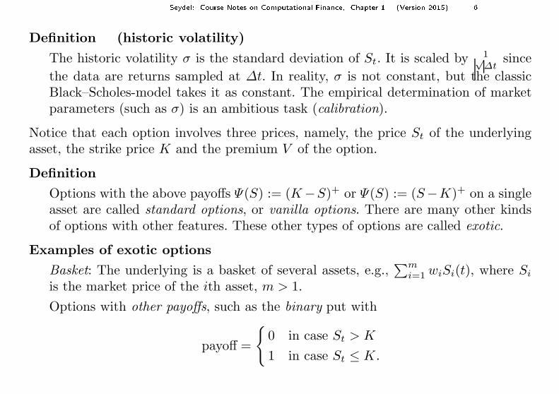
Definition (historic volatility)

The historic volatility σ is the standard deviation of St. It is scaled by 1√∆t

since

the data are returns sampled at ∆t. In reality, σ is not constant, but the classicBlack–Scholes-model takes it as constant. The empirical determination of marketparameters (such as σ) is an ambitious task (calibration).

Notice that each option involves three prices, namely, the price St of the underlyingasset, the strike price K and the premium V of the option.

Definition

Options with the above payoffs Ψ(S) := (K −S)+ or Ψ(S) := (S−K)+ on a singleasset are called standard options, or vanilla options. There are many other kindsof options with other features. These other types of options are called exotic.

Examples of exotic options

Basket: The underlying is a basket of several assets, e.g.,∑m

i=1 wiSi(t), where Si

is the market price of the ith asset, m > 1.

Options with other payoffs, such as the binary put with

payoff =

0 in case St > K

1 in case St ≤ K.


Path dependence: For instance, the payoff ( 1T

∫ T

0S(t) dt−K)+ involves the average

value, which depends on the path of S(t) (average price call).

Barrier: For instance, an option ceases to exist when St reaches a prespecifiedbarrier B.

On the Geometry of options

The values V (S, t) obey the bounds sketched above, see the illustration of an Americanput. V (S, t) can be interpreted as surface (figure: in green) over the half strip 0 ≤ t ≤T, S > 0. This V (S, t) is called value function. At the early-exercise curve, the surfacemerges in the plane defined by the payoff.

K

K

T

0

t

S

V


Importance: When the market price St reaches this (blue) curve, immediate exerciseis optimal: invest K for the interest rate r. The situation is sketched in an (S, t)-planefor an American put that pays no dividend.

t

T

0

SKS

0

For American call options with dividend payment the situation is analogous. Thegeometry at early-exercise curves will be discussed in Chapter 4. The curve must becalculated numerically.


1.2 Mathematical Model

A. Black–Scholes Market

Here we discuss mathematical models of how paths St may behave. We list someassumptions, which essentially go back to Black, Scholes and Merton (1973, Nobel-Prize 1997). These classic assumptions lead to a partial differential equation (PDE),the famous Black–Scholes equation:

∂V

∂t+

1

2σ2 S2 ∂2V

∂S2+ r S

∂V

∂S− r V = 0

This equation is a symbol representing the classic theory. Each solution V (S, t) of aEuropean standard option must solve this PDE, satisfying for t = T the terminalcondition V (S, T ) = Ψ(S) where Ψ denotes the payoff.


Assumptions of the Model

1. There is no arbitrage.

2. The market is frictionless. That is, there are no transaction costs, and rates forlending and borrowing money are equal. All variables are perfectly divisible (∈ IR).And individual trading does affect the market price.

3. The price St follows a geometric Brownian motion (explained later).

4. Technical assumptions:

r and σ are constant for 0 ≤ t ≤ T . No dividends are paid in 0 ≤ t ≤ T .

Provided these assumptions hold (some can be weakened), the value functionof a European standard option solves the Black–Scholes equation. Hence apossible approach to price a European option is to solve the Black–Scholes equation.There is an analytical solution; this is given at the end of this chapter (with δ acontinuous dividend rate).

The above model of a finance market is the classic approach; there are other marketmodels.


The model with its geometric Brownian motion (Section 1.5) is a continuous-timemodel, t ∈ IR. There are also discrete-time models, which consider only discrete timeinstances. Other market models do not use the geometric Brownian motion. Suchmodels are mainly working with jump processes.

Numerical Tasks:

• Computation of V (S, t), in particular for t = 0, with early-exercise curve for Ame-rican options,

• Computation of sensitivities (“Greeks”), such as ∂V (S,0)∂S

,

• Calibration, which means to estimate parameters that match empirical data.

B. Risk-Neutral Probabilities (One-Period Model)Assumptions: 0 < d < u, and the situation of the figure below. There are only

two time instances: 0, T , and two possible future asset prices S0d, S0u. V0 denotes the(unknown) value of the option “today” for t = 0, and S0 is the current value of theasset.


T

0

t

V V (u)

S

V

(d)

S

S S u0 0d

0

0Consider a portfolio with two positions:

1. ∆ shares of the asset

2. a short position of one option written on the asset

With Πt denoting the wealth function, the value Π0 of the portfolio at the time 0 is

Π0 = S0 ∆ − V0 .

The number ∆ is to be determined. At time T the value of the underlying is “up” or“down” and the portfolio is

Π(u) = S0u∆ − V (u)

Π(d) = S0d∆ − V (d) .

V (u) and V (d) are fixed by the payoff. Choose ∆ such that the portfolio becomesriskless at time T . That is, the value of the portfolio should be the same, no matter


whether the market price goes “up” or “down”,

Π(u) = Π(d) =: ΠT .

Consequently,S0∆(u − d) = V (u) − V (d)

or ∆ =V (u) − V (d)

S0u − S0d.

With this special value of ∆ the portfolio is riskless. Invoking the no-arbitrage prin-ciple, we conclude: Any other risk-free investment must have the same value, becauseotherwise arbitrageurs would make a riskless profit by exchanging the investments.Hence: ΠT = Π0 erT

An elementary calculation shows

V0 = e−rT(

V (u)q + V (d)(1 − q))

with q := erT−du−d

. This formula has the structure of an expectation. In case 0 < q < 1

(this requires d < erT < u, a condition guaranteeing absence of arbitrage∗), then thisq induces a probability Q, and

∗ What are the arbitrage strategies in case d ≥ erT or erT ≥ u ?


V0 = e−rT EQ[VT ]

[Recall that in a discrete probability space with a probability P

EP[X] =

n∑

i=1

xi P(X = xi)

holds, where X is a random variable.] The special probability Q defined above is calledrisk-neutral probability. For S0 we have

EQ[ST ] =erT − d

u − d︸︷︷︸

=q

S0u +u − erT

u − d︸︷︷︸

=1−q

S0d = S0erT ,

or

S0 = e−rT EQ[ST ] .


Summary:

In case the portfolio is risk-free (achieved by the above special value of ∆) and

when 0 < q < 1 with q = erT −du−d

, then there is a probability Q, such that

V0 = e−rT EQ[VT ] and

S0 = e−rT EQ[ST ] .

The quantity ∆ is called Delta. Later we shall see ∆ = ∂V∂S

in the time-continuoussituation. This is the first and most important example of the “Greeks”, others are∂2V∂S2 , ∂V

∂σ, ...

∆ is the key for “Delta-Hedging”, for minimizing or eliminating the risk of thewriter of an option.

Remark: The relatione−rT EQ[ST ] = S0

for all T is the martingale property of the discounted process e−rtSt with respect tothe probability Q.


1.3 Binomial Method

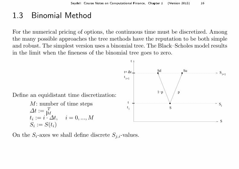
For the numerical pricing of options, the continuous time must be discretized. Amongthe many possible approaches the tree methods have the reputation to be both simpleand robust. The simplest version uses a binomial tree. The Black–Scholes model resultsin the limit when the fineness of the binomial tree goes to zero.

−

t i+1

t i

Si+1

Si

t+ ∆t

p1−p

SuSd

t

S

t

S

Define an equidistant time discretization:

M : number of time steps∆t := T

M

ti := i · ∆t, i = 0, ...,MSi := S(ti)

On the Si-axes we shall define discrete Sj,i-values.


Assumptions

(Bi1)The market price over one period ∆t can only take two values,

Su or Sd with 0 < d < u.

(Bi2)Let the probability of an “up” motion be p, P(up) = p, with 0 < p < 1.

(Bi3)Expectation and variance equal those of the continuous-time model (for geometricBrownian motion St with riskless growth rate r).

(Bi1) and (Bi2) define the framework of a binomial process with probability. The freeparameters u, d, p are to be determined such that (Bi1) – (Bi3) hold.

Remarks

1. It turns out that P is the risk-neutral probability Q. Literature on the stocha-stic background: [Musiela&Rutkowski: Martingale Methods in Financial modeling],[Shreve: Stochastic Calculus for Finance II (Continuous-time models)].

2. In Section 1.5D we shall show for the continuous-time Black–Scholes model

E[St] = S0er(t−t0)

E[S2t ] = S2

0e(2r+σ2)(t−t0)

Set Si for S0, Si+1 for St and ∆t for t − t0.


3. The expectations are conditional expectations since the initial values S(t0) or Si

are given.

Conclusion for the step i −→ i + 1:

E[S(ti+1) | S(ti) = Si] = Sier∆t

Var[S(ti+1) | S(ti) = Si] = S2i e2r∆t(eσ2∆t − 1)

The expectation of the discrete model is

E[Si+1] = p Siu + (1 − p) Sid.

Equating with the expression of the continuous-time model shows

er∆t = pu + (1 − p)d .

This is the first equation for the three unknowns u, d, p. This gives

p =er∆t − d

u − d.

For 0 < p < 1 we required < er∆t < u .


This must hold because otherwise arbitrage is possible. (Compare with Section 1.2Bto see that p is the q and represents the risk-neutral probability.)

Equating variances leads to

Var[Si+1] = E[S2i+1] − (E[Si+1])

2

= p (Siu)2 + (1 − p) (Sid)2 − S2i (pu + (1 − p)d)2

!= S2

i e2r∆t(eσ2∆t − 1) ,

which amounts toe2r∆t+σ2∆t = pu2 + (1 − p)d2.

A third equation can be posed arbitrarily. For example, a kind of symmetry is expressedby

u · d = 1.


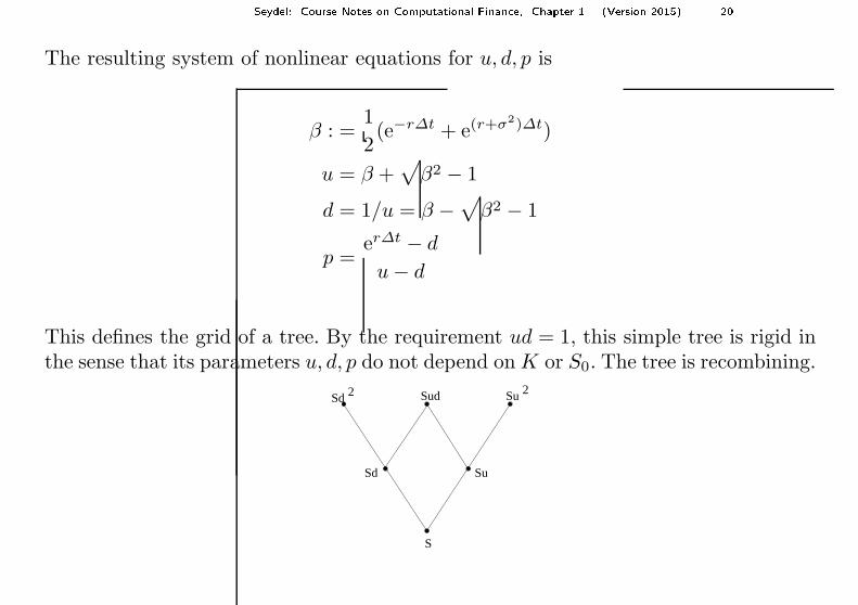
The resulting system of nonlinear equations for u, d, p is

β : =1

2(e−r∆t + e(r+σ2)∆t)

u = β +√

β2 − 1

d = 1/u = β −√

β2 − 1

p =er∆t − d

u − d

This defines the grid of a tree. By the requirement ud = 1, this simple tree is rigid inthe sense that its parameters u, d, p do not depend on K or S0. The tree is recombining.

2

S

Sd Su

Sd Sud Su2


Since Si+1 = αSi, α ∈ u, d the “branches” of the tree grow exponentially.

0

0.05

0.1

0.15

0.2

0.25

0.3

0.35

0.4

0.45

0 50 100 150 200 250

S

T

The S-values of the grid are

Sj,i := S0ujdi−j , j = 0, ..., i, i = 1, ...,M.


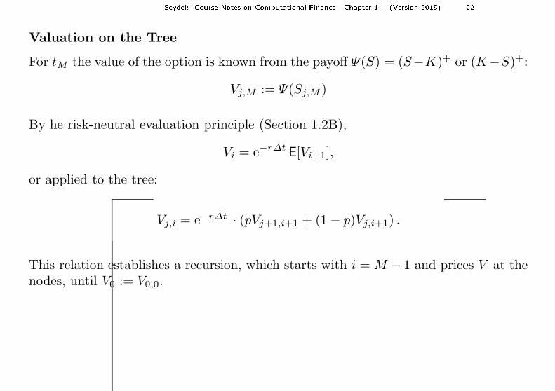
Valuation on the Tree

For tM the value of the option is known from the payoff Ψ(S) = (S−K)+ or (K−S)+:

Vj,M := Ψ(Sj,M )

By he risk-neutral evaluation principle (Section 1.2B),

Vi = e−r∆t E[Vi+1],

or applied to the tree:

Vj,i = e−r∆t · (pVj+1,i+1 + (1 − p)Vj,i+1) .

This relation establishes a recursion, which starts with i = M − 1 and prices V at thenodes, until V0 := V0,0.


In case of an American option, each node requires a check whether early exercise isreasonable. The holder of the option optimizes her position by comparing the payoffΨ(S) with the continuation value: she chooses the larger value. This requires to modifythe above recursion. We denote the continuation value

V contj,i := e−r∆t (pVj+1,i+1 + (1 − p)Vj,i+1).

For European options Vj,i := V contj,i .

For American options Vj,i := maxΨ(Sj,i), V contj,i , or

call: Vj,i := max(Sj,i − K)+, V contj,i

put: Vj,i := max(K − Sj,i)+, V cont

j,i (principle of dynamic programming)

The two different decisions, either holding or exercising the American-style option, havea geometrical aspect: In the (S, t)-plane the nodes with V cont

j,i > Ψ(Sj,i) characterizethe continuation area, and the other nodes are in the stopping area. How the early-exercise curve separates the two areas will be discussed in Chapter 4.


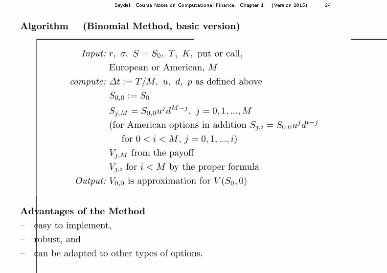
Algorithm (Binomial Method, basic version)

Input: r, σ, S = S0, T, K, put or call,

European or American, M

compute: ∆t := T/M, u, d, p as defined above

S0,0 := S0

Sj,M = S0,0ujdM−j , j = 0, 1, ...,M

(for American options in addition Sj,i = S0,0ujdi−j

for 0 < i < M , j = 0, 1, ..., i)

Vj,M from the payoff

Vj,i for i < M by the proper formula

Output: V0,0 is approximation for V (S0, 0)

Advantages of the Method

– easy to implement,

– robust, and

– can be adapted to other types of options.


Disadvantages of the Method

– accuracy is rather poor:

error O(1/M) = O(∆t), which is linear convergence. (But the accuracy matchespractical requirements.)

– In case V0 is needed for several values of S, the algorithm must be restarted.

Enhancements

– To avoid oscillations, generalize ud = 1 to ud = γ and choose γ such that for t = Tone node of the tree falls on the strike value K. Then the parameters depend onK and S0, resulting in a more flexible tree and improved accuracy.

– Discrete dividend payment at time tD: Cut the tree at tD and shift the S-valuesby −D. As result, evaluate the tree at S0 := S0 − De−rtD . (Illustrations in Topic1 and 5 in the Topics for CF.)

– Sensitivities (“greeks”) are calculated by difference quotients.

Problems

In the higher-dimensional case (e.g. basket option with three or more assets) it isnot obvious how to generalize the tree.In the literature the above method is often called Cox-Ross-Rubinstein method(CRR). Other extensions: trinomial method; “implied grid” for variable σ(S, t).


1.4 Stochastic Processes

This section introduces continuous-time models as they are used by Black, Scholes andMerton. Essentially we discuss (geometric) Brownian motion.

History

Brown (1827): studied erratic motion of pollen.

Bachelier (1900): applied Brownian motion to model asset prices.

Einstein (1905): molecular motion

Wiener (1923): mathematical model

since 1940: Ito and others

Definition (Stochastic Process)

A stochastic process is a family of random variables Xt for t ≥ 0 or 0 ≤ t ≤ T .

Each sample results in a function Xt called path or trajectory.

Definition (Wiener process / standard Brownian motion)

Wt (notation also W (t) or W or Wtt≥0) has the properties:

(a) Wt is a continuous stochastic process


(b) W0 = 0

(c) Wt ∼ N (0, t)

(d) All increments ∆Wt := Wt+∆t − Wt (∆t arbitrary) on non-overlapping t-intervals are independent.

(c) means: Wt is distributed normally with E[Wt] = 0 and Var[Wt] = E[W 2t ] = t.

Remarks

1) “standard”, because it is scalar, driftless, and W0 = 0.Xt = a + µt + Wt with a, µ ∈ IR is the general Brownian motion (with drift µ).

2) Consequences (also for W0 = a):

E[Wt − Ws] = 0 , Var[Wt − Ws] = t − s for t > s .

(show this as exercise)

3) Wt is nowhere differentiable! Motivation:

Var

[∆Wt

∆t

]

=1

(∆t)2Var[∆Wt] =

(1

∆t

)2

· ∆t =1

∆t

tends to ∞ for ∆t → 0.


4) A Wiener process is self-similar in the sense:

Wβtd=

√

β Wt

(both sides obey the same distribution). More general, there are fractal Wienerprocesses with

Wβtd= βHWt ,

for the standard Wiener process H = 12 . H is the Hurst-exponent. Mandelbrot

postulated that finance models should use fractal processes.

Importance

The Wiener process is “driving force” of basic finance models.

Discretization/Computation

So far we have considered Wt for continuous-time models (t ∈ IR). Now we appro-ximate W by a discretization. Take ∆t > 0 as a fixed time increment.

tj := j · ∆t ⇒ Wj∆t =

j∑

k=1

(Wk∆t − W(k−1)∆t) =

j∑

k=1

∆Wk

The ∆Wk are independent, and by Remark 2 satisfy


E(∆Wk) = 0, Var(∆Wk) = ∆t.

In case Z is a random variable with Z ∼ N (0, 1) [Chapter 2], then

Z√

∆t ∼ N (0,∆t).

HenceZ ·

√∆t for Z ∼ N (0, 1)

serves as model for the process of the ∆Wk.

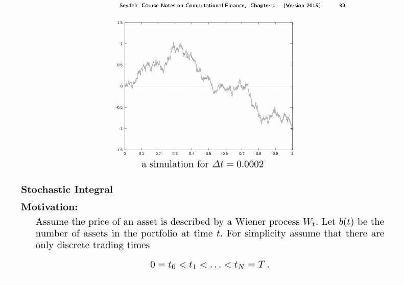
Algorithm (Simulation of a Wiener process)

start: t0 = 0, W0 = 0; choose ∆t .

loop j = 1, 2, ... :

tj = tj−1 + ∆t

draw Z ∼ N (0, 1)

Wj = Wj−1 + Z√

∆t

The Wj denotes a realization of Wt at tj .


-1.5

-1

-0.5

0

0.5

1

1.5

0 0.1 0.2 0.3 0.4 0.5 0.6 0.7 0.8 0.9 1

a simulation for ∆t = 0.0002

Stochastic Integral

Motivation:

Assume the price of an asset is described by a Wiener process Wt. Let b(t) be thenumber of assets in the portfolio at time t. For simplicity assume that there areonly discrete trading times

0 = t0 < t1 < . . . < tN = T .


Hence b(t) is piecewise constant:

b(t) = b(tj−1) for tj−1 ≤ t < tj . (∗)

The resulting trading gain is

N∑

j=1

b(tj−1)(Wtj− Wtj−1

) for 0 ≤ t ≤ T.

Now we approach the time-continuous case and assume arbitrary trading times. Thequestion is whether the sum converges for N → ∞?

For arbitrary b the integral∫ T

0

b(t) dWt

does not exist as Riemann–Stieltjes integral. Sufficient for its existence would be afinite first variation of Wt.

We show: The first variationN∑

j=1

|Wtj− Wtj−1

| is unbounded.


Proof: Clearly

N∑

j=1

|Wtj− Wtj−1

|2 ≤ maxj

(|Wtj− Wtj−1

|)N∑

j=1

|Wtj− Wtj−1

|

for any decomposition of the interval [0, T ]. Now ∆t → 0. The second variation isbounded, it converges to a c 6= 0 (see the Lemma below). By the continuity of Wt,the first factor of the right-hand side goes to 0, and hence the second factor (thefirst variation) to ∞.

It remains to investigate what happens with the second variation. The relevant typeof convergence is convergence in the mean,

limN→∞

E[(X − XN )2] = 0 ,

written as: X = l.i.m.N→∞

XN .

It remains to show:


Lemma

Denote by t0 = t(N)0 < t

(N)1 < . . . < t

(N)N = T a sequence of partitions of the

interval t0 ≤ t ≤ T , with δN :=N

maxj=1

(t(N)j − t

(N)j−1). Then:

l.i.m.δN→0

N∑

j=1

(Wt(N)j

− Wt(N)j−1

)2 = T − t0

Proof: Exercises

Remark: Part of the proof of the lemma comprises the assertions

E[(∆Wt)2 − ∆t] = 0

Var[(∆Wt)2 − ∆t] = 2 · (∆t)2.

In this probabilistic sense the random variable ∆W 2t behaves similarly as ∆t. Symbo-

lically this is written

(dWt)2 = dt

and will be used for investigations of orders of magnitude.


The construction of an integral for our integrands b

t∫

t0

b(s) dWs

is based on∫ t

t0b(s)dWs :=

∑Nj=1 b(tj−1)(Wtj

− Wtj−1) for all step functions b in the

sense of (∗).For more general b we take step functions converging to b in the mean. For literaturesee [Øksendal: Stochastic Differential Equations], [Shreve: Stochastic Calculus].


1.5 Stochastic Differential Equations

A. Integral Equation

Definition (Diffusion model)

The integral equation

Xt = Xt0 +

∫ t

t0

a(Xs, s) ds +

∫ t

t0

b(Xs, s) dWs

for a stochastic process Xt is called Ito stochastic differential equation (SDE). Itssymbolic notation is

dXt = a(Xt, t) dt + b(Xt, t) dWt

Solutions of this stochastic differential equation (that is, of the integral equation) arecalled stochastic diffusion, or Ito-process. The term a(Xt, t) is the drift term, andb(Xt, t) is the diffusion.

Special cases

- The Wiener process is included with Xt = Wt, a = 0, b = 1.

- In the deterministic case b = 0 holds, i.e. dXt

dt= a(Xt, t).


Algorithm (analogous as for the Wiener process)

is based on the discrete version

∆Xt = a(Xt, t)∆t + b(Xt, t)∆Wt

with increments ∆W and ∆t as in Section 1.4. Let yj denote an approximation ofXtj

.

Start: t0, y0 = X0 ; choose ∆t .

loop: j = 0, 1, 2, ...

tj+1 = tj + ∆t

∆W = Z√

∆t with Z ∼ N (0, 1)

yj+1 = yj + a(yj , tj)∆t + b(yj , tj)∆W

Since dW 2 = dt, we expect an order of only 12 ; we come back to this in Chapter 3.


B. Application to the Stock Market

Model (GBM = geometric Brownian motion)

dSt = µSt dt + σSt dWt

This is an Ito-stochastic SDE with a = µSt and b = σSt. This SDE is linear as longas µ and σ do not depend on St. For Black and Scholes µ and σ are constant.

(This fills the gap GBM in Assumption 3 in Section 1.2 in the market model.)

µ is interpreted as growth rate, and σ as volatility. The relative change is describedby

dSt

St

= µ dt + σ dWt .

The classic theory of Black, Scholes and Merton (and a significant part of this chapter)assumes a GBM with constant µ, σ.

(Bachelier’s model wasdSt = µ dt + σ dWt ;

here the price St can become negative.)


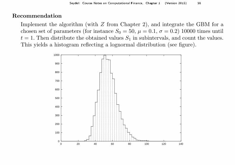
Recommendation

Implement the algorithm (with Z from Chapter 2), and integrate the GBM for achosen set of parameters (for instance S0 = 50, µ = 0.1, σ = 0.2) 10000 times untilt = 1. Then distribute the obtained values S1 in subintervals, and count the values.This yields a histogram reflecting a lognormal distribution (see figure).

0

100

200

300

400

500

600

700

800

900

1000

0 20 40 60 80 100 120 140


Consequence:

From∆S

S= µ∆t + σ ∆W

we conclude for the distribution of the ∆SS

:

1) distributed normally

2) E[∆SS

] = µ∆t

3) Var[∆SS

] = σ2∆t

together: ∆SS

∼ N (µ∆t, σ2∆t)

This offers a way to calculate volatilities σ empirically: For a sequence of trading dayscollect the data ∆S

S, call them Ri (returns), where Ri+1 and Ri are measured at time

distance ∆t. Assuming that GBM is appropriate to describe the returns, σ is obtainedas

σ =1√∆t

∗ standard deviation of the Ri .

This specific value of σ, based on data of the past, is called historic volatility (for theimplied volatility see the Exercises.)

S under GBM can be approximated by the above algorithm as long as ∆t > 0 is smallenough, and S > 0.


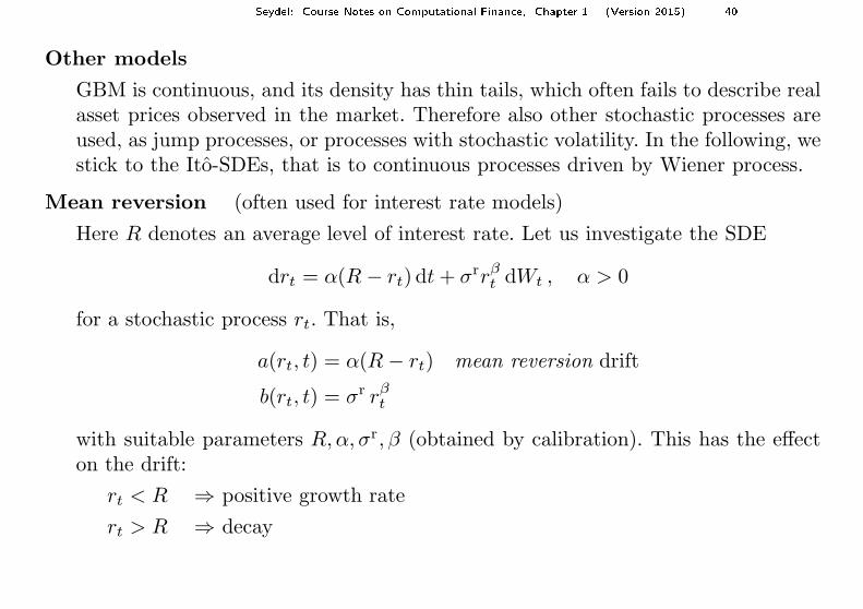
Other models

GBM is continuous, and its density has thin tails, which often fails to describe realasset prices observed in the market. Therefore also other stochastic processes areused, as jump processes, or processes with stochastic volatility. In the following, westick to the Ito-SDEs, that is to continuous processes driven by Wiener process.

Mean reversion (often used for interest rate models)

Here R denotes an average level of interest rate. Let us investigate the SDE

drt = α(R − rt) dt + σrrβt dWt , α > 0

for a stochastic process rt. That is,

a(rt, t) = α(R − rt) mean reversion drift

b(rt, t) = σr rβt

with suitable parameters R,α, σr, β (obtained by calibration). This has the effecton the drift:

rt < R ⇒ positive growth rate

rt > R ⇒ decay


This effect is superseded by the stochastic fluctuations, but essentially the meanreversion takes care that the order of magnitude of rt stays close to R, or revertsto R. The parameter α controls the intensity of the reversion.

For β = 12 , i.e. b(rt, t) = σr√rt, the model is called CIR model (Cox-Ingersoll-

Ross model).

Figure: A simulation rt of the Cox-Ingersoll-Ross model for R = 0.05, α = 1, β = 0.5,r0 = 0.15, σr = 0.1, ∆t = 0.01

0

0.02

0.04

0.06

0.08

0.1

0.12

0.14

0.16

0 1 2 3 4 5 6 7 8 9 10


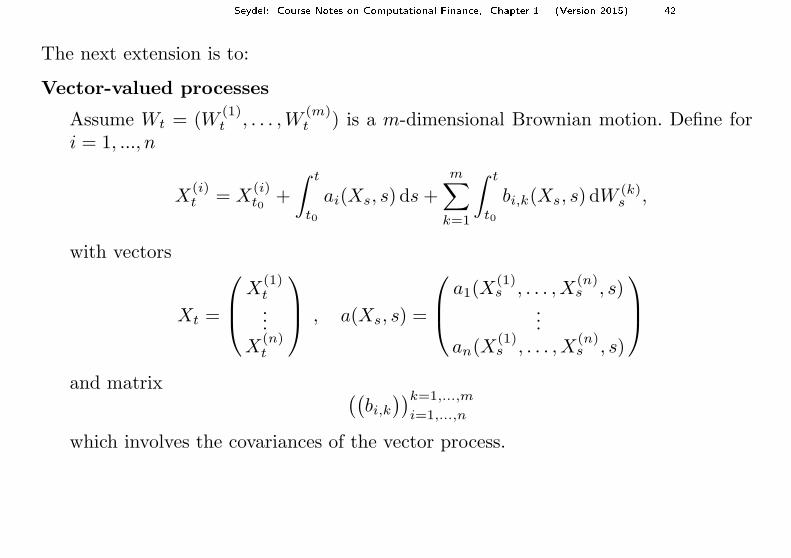
The next extension is to:

Vector-valued processes

Assume Wt = (W(1)t , . . . ,W

(m)t ) is a m-dimensional Brownian motion. Define for

i = 1, ..., n

X(i)t = X

(i)t0

+

∫ t

t0

ai(Xs, s) ds +

m∑

k=1

∫ t

t0

bi,k(Xs, s) dW (k)s ,

with vectors

Xt =

X(1)t...

X(n)t

, a(Xs, s) =

a1(X(1)s , . . . ,X

(n)s , s)

...an(X

(1)s , . . . ,X

(n)s , s)

and matrix((

bi,k

))k=1,...,m

i=1,...,n

which involves the covariances of the vector process.


Example 1 Heston’s model

dSt = µSt dt +√

vtSt dW (1)

dvt = κ(θ − vt) dt + σvola√

vt dW (2)

The stochastic volatility√

vt is defined via a mean reversion for the variance vt.

This model (with n = 2 and m = 2) involves parameters κ, θ, σvola, the correlationρ between W (1) and W (2), an initial value v0 and a growth rate µ which may begiven by a risk-free valuation concept. Altogether, about five parameters must becalibrated. Heston’s model is used frequently.


Example 2 volatility tandem

dS = σS dW (1)

dσ = −(σ − ζ)dt + ασ dW (2)

dζ = β(σ − ζ) dt

0.12

0.14

0.16

0.18

0.2

0.22

0.24

0.26

0 0.2 0.4 0.6 0.8 1

α = 0.3, β = 10; dashed: ζ

Hint: local volatility meansσ = σ(t, St).


C. Ito Lemma

Motivation (deterministic case)

Suppose x(t) is a function, and y(t) := g(x(t), t). The chain rule implies

d

dtg =

∂g

∂x· dx

dt+

∂g

∂t.

With dx = a(x(t), t)dt this can be written

dg =

(∂g

∂xa +

∂g

∂t

)

dt

Lemma (Ito)

Assume Xt is an Ito process following dXt = a(Xt, t) dt+b(Xt, t) dWt and g(x, t) ∈C2. Then Yt := g(Xt, t) solves the SDE

dYt =

(∂g

∂xa +

∂g

∂t+

1

2

∂2g

∂x2b2

)

dt +∂g

∂xb dWt .

That is, Yt is an Ito process with the same Wiener process as the input process Xt.


Sketch of a proof:

t → t + ∆t

X → X + ∆X

→ g(X + ∆X, t + ∆t) = Y + ∆Y

Taylor expansion of g leads to ∆Y :

∆Y =∂g

∂X· ∆X +

∂g

∂t∆t + terms quadratic in ∆t,∆X

Substitute∆X = a∆t + b∆W

(∆X)2 = a2 ∆t2 + b2 ∆W 2︸︷︷︸

=O(∆t)

+2ab∆t∆W

and order the terms according to powers of ∆t, ∆W to obtain

∆Y =

(∂g

∂Xa +

∂g

∂t+

1

2

∂2g

∂X2b2

)

∆t + b∂g

∂X∆W + t.h.o.

Similar as in Section 1.4, ∆W can be written as sum, and convergence in the mean isapplied. See [Øksendal].


D. Application to the GBM model

Assume the GBM modeldS = µS dt + σS dW

with µ and σ constant, i.e. X = S, a = µS, b = σS.

1) Let V (S, t) be smooth (∈ C2)

⇒ dV =

(∂V

∂SµS +

∂V

∂t+

1

2σ2S2 ∂2V

∂S2

)

dt +∂V

∂SσS dW

This is the basic SDE which leads to the PDE of Black and Scholes for thevalue function V (S, t) of a European standard option.

2) Yt := log(St), i.e. g(x) = log x

⇒ ∂g

∂x=

1

xand

∂2g

∂x2= − 1

x2

⇒ d (log St) =

(

µ − σ2

2

)

dt + σ dWt

Hence the log-prices Yt = log St satisfy a simple SDE, with the elementarysolution:


Yt = Yt0 +

(

µ − σ2

2

)

(t − t0) + σ(Wt − Wt0)

⇒ log St − log St0 = logSt

St0

=

(

µ − σ2

2

)

(t − t0) + σ(Wt − Wt0)

⇒ St = St0 · exp

[(

µ − σ2

2

)

(t − t0) + σ(Wt − Wt0)

]

For t0 = 0 and Wt0 = W0 = 0, this results in

St = S0 exp[(

µ − σ2

2

)

t + σWt

]

In summary, St is exponential function of a Brownian motion with drift.

Implications for t0 = 0:

a) log St is distributed normally

b) E[log St] = E[log S0] + (µ − σ2

2 )t + 0 = log S0 + (µ − σ2

2 )t

c) Var[log St] = Var[σWt] = σ2t

summarizing a) – c) means


logSt

S0∼ N

(

(µ − σ2

2)t , σ2t

)

d) This leads to the density function of Y = log S

f(Y ) = f(log St) =1

σ√

2πtexp

[

− (log(St/S0) − (µ − σ2/2)t)2

2σ2t

]

.

And what is the density of St? The probabilities of S and Y are the same and hencealso the distribution integrals. We apply the transformation theorem (Section 2.2B)for Y := log S and have the integrands

f(Y ) dY = f(log S)1

S︸︷︷︸

f(St)

dS.

Consequently, the density f of the distribution of the asset price St is

f(St, t; S0, µ, σ) :=1

Stσ√

2πtexp

[

− (log(St/S0) − (µ − σ2/2)t)2

2σ2t

]

.

This is the density fGBM of the lognormal distribution. It describes the probabilityof the transition (S0, 0) −→ (St, t) under GBM.


e) Now the last gap in the derivation of the binomial method can be closed: Therethe continuous model refers to our GBM. As an exercise, realize

E(S) =

∞∫

0

Sf(. . .) dS = S0 eµ(t−t0)

E(S2) =

∞∫

0

S2f(. . .) dS = S20 e(σ2+2µ)(t−t0)


1.6 Risk-Neutral Valuation

(This section sketches basic ideas and concepts. For a thorough treatment we re-commend literature on Stochastic Finance such as [Musiela&Rutkowski: MartingaleMethods in Financial modeling])

Recall (from the one-period)

V0 = e−rT EQ[Ψ(ST )]

where Q is the artificial probability of Section 1.2 and Ψ(ST ) denotes the payoff.

For the model with continuous time formally the same relation holds. But Q andEQ are different. It turns out that the density of Q is given by f(St, t; S0, r, σ), withµ replaced by r. Hence the relation

V0 = e−rT

∫ ∞

0

Ψ(ST ) · f(ST , T ; S0, r, σ) dST

holds for the GBM-based continuous model. In the following we outline the argumentsthat lead to this integral.


Fundamental Theorem of Asset Pricing

The market model is free of arbitrage if and only if there is a probability Q suchthat the discounted asset prices e−rtSt are martingales with respect to Q.

Probability space

The same sample space and σ-algebra (Ω,F) underlying a Wiener process arenot specified. The chosen probability P completes (Ω,F) to the probability space(Ω,F ,P). The independence of the increments ∆W of the Wiener process dependon P. A process W can be a Wiener process with respect to P, but is no Wienerprocess with respect to another probability P

Martingale

A martingale Mt is a stochastic process with

E[Mt | Fs] = Ms for all t, s with s ≤ t ,

where Fs is a filtration, i.e. a family of σ-algebras with Fs ⊆ Ft ∀s ≤ t. A filtrationserves as model for the amount of information in a market.

E[Mt | Fs] is a conditional expectation. It can be regarded as expectation of Mt

conditional on the amount of information available until time instant s.

Mt martingale means that Ms at time s is the best possible forecast for t ≥ s.


Martingale with respect to a probability Q: EQ[Mt | Fs] = Ms for all t, s with s ≤ t.

Examples of martingales

1) any Wiener process

2) W 2t − t for any Wiener process W .

3) A necessary criterion for martingales is the absence of drift.

Essentially, drift-free processes are martingales.

Market Price of Risk

dS = µS dt + σS dW

= rS dt + (µ − r)S dt + σS dW

= rS dt + σS

[µ − r

σdt + dW

]

The investor expects µ > r as a compensation for the risk, which is represented by σ.µ − r is the excess return.

γ :=µ − r

σ= “market price of risk”

= compensation rate relative to the risk


HencedS = rS dt + σS [γ dt + dW ] . (∗)

Under the probability P the term in brackets represents a drifted Brownian motionand no (standard) Wiener process.

Girsanov’s Theorem

Suppose W is Wiener process with respect to (Ω,F ,P). In case γ satisfies certainrequirements, there is a probability Q such that

W γt := Wt +

∫ t

0

γ ds

is a (standard) Wiener process under Q.

(probability theory: Q results from the Theorem of Radon-Nikodym. Q and P areequivalent. For constant γ the requirements of Girsanov are fulfilled.)

Application

Substitute dW γ = dW + γdt in (∗) gives

dS = rS dt + σS dW γ.


This is a change of drift from µ to r; σ remains unchanged. The path of St under theprobability Q is defined by the density f(. . . , r, σ). The transition from f(. . . , µ, σ)to f(. . . , r, σ) amounts to adjusting the probability from P to Q. The discountede−rtSt is drift-free under Q and Martingale. Q is called “risk-neutral” probability.

Trading Strategy

Let Xt be a stochastic vector process of market prices, and bt denotes the vectorwith the numbers of shares held in the portfolio. Hence btr

t Xt is the wealth processof the portfolio.

Example

Xt :=

(St

Bt

)

,

where St is the market price of the asset underlying an option, and Bt is the valueof a risk-free bond.


Notation: Vt is the random variable of the value of an European option.Assumptions:

(1) There is a strategy bt replicating the payoff of the option at time T ,

btrT XT = Payoff .

bt must be Ft-measurable for all t. (That is, the trader cannot see the future.Note that the value of the payoff is a random variable.)

(2) The portfolio is closed, no money is inserted or withdrawn. This is the self-financing property defined as

d(btrt Xt) = btr

t dXt .

(3) The market is free of arbitrage.

(1), (2), (3) ⇒ Vt = btrt Xt for 0 ≤ t ≤ T (otherwise there would exist arbitrage)

We consider a European option and a discounting process Yt with the property thatYtXt is martingale. Then one can show that also Ytb

trt Xt is martingale (both with

respect to Q).


Implications for European options for t ≤ T

YtVt = Ytbtrt Xt = EQ[YT btr

T XT | Ft] (martingale)= EQ[YT · Payoff | Ft] (replication)

When the payoff is a function Ψ of ST (vanilla-option under GBM), then

= EQ[YT · Ψ(ST )]

(because WT − Wt is independent of Ft). Discounting with Yt = e−rt impliesspecifically for t = 0

1 · V0 = EQ[e−rT · Ψ(ST )]

and hence

V0 = e−rT

∫ ∞

0

Ψ(ST ) · f(ST , T ; S0, r, σ) dST .

This is called risk-neutral valuation.


Literature on Stochastic Finance: [Elliot & Kopp: Mathematics of Financial Markets],[Korn: Option Pricing and Portfolio Optimization], [Musiela & Rutkowski: MartingaleMethods in Financial modeling], [Shreve: Stochastic Calculus for Finance].

Outlook

We so far have investigated continuous processes St driven by Wt. To compensatefor occasional drastic changes in the price of underlying, one resorts to models withstochastic volatility, or to jump processes.

Supplements

The “Greeks” mean the sensitivities of V (S, t; σ, r) and are defined as

Delta =∂V

∂S, gamma =

∂2V

∂S2, theta =

∂V

∂t, vega =

∂V

∂σ, rho =

∂V

∂r


Black–Scholes Formula

For a European call the analytic solution of the Black–Scholes equation is

d1 :=log S

K+

(

r − δ + σ2

2

)

(T − t)

σ√

T − t

d2 := d1 − σ√

T − t =log S

K+

(

r − δ − σ2

2

)

(T − t)

σ√

T − t

VC(S, t) = Se−δ(T−t)F (d1) − Ke−r(T−t)F (d2),

where F denotes the standard normal cumulative distribution (compare Exercises),and δ is a continuous dividend yield. The value VP(S, t) of a put is obtained by applyingthe put-call parity

VP = VC − Se−δ(T−t) + Ke−r(T−t)

from whichVP = −Se−δ(T−t)F (−d1) + Ke−r(T−t)F (−d2)

follows.

modelling financial options

Documents