modelling approaches for the assessment of projected ... approaches... · 2.2 towards qualitative...
TRANSCRIPT

This project has received funding from the European Union’s Horizon 2020 research and innovation
programme under grant agreement No 642317.
Modelling approaches for the
assessment of projected impacts of
drivers of change on biodiversity,
ecosystems functions and aquatic
ecosystems service delivery
Deliverable 7.1

Authors
Sami Domisch, Simone D. Langhans, Virgilio Hermoso, Sonja C. Jähnig, Karan Kakouei (FVB-
IGB)
Javier Martínez-López, Stefano Balbi, Ferdinando Villa (BC3)
Nele Schuwirth, Peter Reichert, Mathias Kuemmerlen, Peter Vermeiren (Eawag)
Leonie Robinson, Fiona Culhane (ULIV)
Antonio Nogueira, Heliana Teixeira, Ana Lillebø (UAVR)
Andrea Funk, Florian Pletterbauer, Daniel Trauner, Thomas Hein (BOKU)
Maja Schlüter, Romina Martin, Katharina Fryers Hellquist (SRC)
Gonzalo Delacámara, Carlos M. Gómez (IMDEA)
Gerjan Piet, Ralf van Hal (WMR)
With thanks to: Davide Geneletti (University of Trento, AQUACROSS Science-Policy-Business
Think Tank), Manuel Lago, Katrina Abhold and Lina Röschel (ECOLOGIC)
Project coordination and editing provided by Ecologic Institute.
Manuscript completed in July, 2017
Document title Modelling approaches for the assessment of projected impacts of
drivers of change on biodiversity, ecosystems functions and aquatic
ecosystems service delivery
Work Package WP7
Document Type Public Deliverable
Date July 2017 (original submission), June2018 (revised submission)
Acknowledgments & Disclaimer
This project has received funding from the European Union’s Horizon 2020 research and
innovation programme under grant agreement No 642317.
Neither the European Commission nor any person acting on behalf of the Commission is
responsible for the use which might be made of the following information. The views
expressed in this publication are the sole responsibility of the author and do not necessarily
reflect the views of the European Commission.
Reproduction and translation for non-commercial purposes are authorised, provided the
source is acknowledged and the publisher is given prior notice and sent a copy.

Suggested Citation: Domisch, S., Langhans, S.D., Hermoso, V., Jähnig, S.C., Kakouei, K.,
Martínez-López, J., Balbi, S., Villa, F., Schuwirth, N., Reichert, P., Kuemmerlen, M., Vermeiren,
P., Robinson, L., Culhane, F., Nogueira, A., Teixeira, H., Lillebø, A., Funk, A., Pletterbauer, F.,
Trauner, D., Hein, T. Schlüter, M., Martin, R., Fryers Hellquist, K. Delacámara, G., Gómez, C.M.,
Piet, G., van Hal, R. (2017). “Modelling approaches for the assessment of projected impacts of
drivers of change on biodiversity, ecosystems functions and aquatic ecosystems service
delivery: AQUACROSS Deliverable 7.1”, European Union’s Horizon 2020 Framework
Programme for Research and Innovation Grant Agreement No. 642317.

Table of Contents
Table of Contents 1
About AQUACROSS 2
1 Background 3
2 Introduction 5
2.1 Current state of knowledge 5
2.2 Towards qualitative and quantitative models of biodiversity,
ecosystem functions and services 7
3 Qualitative Models: The Linkage Framework 9
3.1 Linkage matrices: a first step for coupling biodiversity and
ecosystem services 9
3.2 Linkage framework: a series of connected matrices 10
4 Quantitative Models: A Spatially-explicit Modelling Framework 16
4.1 Data requirements 19
4.1.1 Biodiversity component 19
4.1.2 Ecosystem services component 21
4.1.3 Spatial prioritisation 22
4.2 Data structure and spatial units 23
4.3 Model components and types 24
4.3.1 Biodiversity models 24

4.3.2 Ecosystem service models 29
4.3.3 Systematic spatial prioritisation tools 40
5 Scenarios 48
5.1 Types of scenarios within AQUACROSS 48
5.2 Scenarios in the case studies 49
6 Model Coupling: Combining Biodiversity, Ecosystem Functions and
Ecosystem Services within the Spatial Prioritisation 51
6.1 Iterate, adjust and predict models under different scenarios 52
6.2 Advantages of the spatial modelling framework 53
7 Assessing Uncertainties 54
8 Alternatives 54
8.1 Alternatives within the modelling framework 55
8.2 Semi-quantitative risk-based approach 56
9 Outlook 59
10 References 60
List of Tables
Table 1: CICES typology of ESS and abiotic outputs, taken from Nogueira et al. (2016;
Deliverable 5.1) 12
Table 2: Typology of ecosystem components (habitats and biotic groups) for European
aquatic ecosystems 15
Table 3: Stand-alone software for building Species Distribution Models 28

Table 4: List of criteria used for assessing various criteria of ecosystem service models
from a user’s perspective 34
Table 5: Summary of the ecosystem service tools’ features 35
Table 6: Examples of Marxan applications in aquatic realms in the literature 42
Table 7: Examples of Marxan with Zones applications in aquatic realms in the
literature 43
Table 8: The pressure assessment criteria and categories used to evaluate each impact
chain and the numerical risk scores assigned to each category 58
List of Figures
Figure 1: The AQUACROSS Assessment Framework sequence 4
Figure 2: Generic workflow of the qualitative and quantitative (spatial) modelling. 8
Figure 3: Workflow for evaluating action strategies and prioritising conservation and
ecosystem services delivery areas for the application in the AQUACROSS case studies
17
Figure 4: Schematic overview of spatial units for the modelling workflow 23
Figure 5: Schematic workflow of species distribution models 25
List of Boxes
Box 1: Lessons learnt on drivers of change and pressures on aquatic ecosystems. 6
Box 2: A detailed description of the single components of the proposed spatial
modelling workflow as shown in Figure 3 18

List of abbreviations
ARIES Artificial Intelligence for Ecosystem Services
BBN Bayesian Belief Network
CBD Convention on Biological Diversity
EBM Ecosystem-based management
EF Ecosystem function
ESS Ecosystem services
IPBES Intergovernmental Science-Policy Platform on Biodiversity and
Ecosystem Services
MAES Mapping and Assessment of Ecosystems and their Services
PU Planning unit
SDM Species Distribution Model
WP Work Package

2 Deliverable 7.1
About AQUACROSS
Knowledge, Assessment, and Management for AQUAtic Biodiversity and Ecosystem
Services aCROSS EU policies (AQUACROSS) aims to support EU efforts to protect
aquatic biodiversity and ensure the provision of aquatic ecosystem services. Funded
by Europe's Horizon 2020 research programme, AQUACROSS seeks to advance
knowledge and application of ecosystem-based management for aquatic ecosystems
to support the timely achievement of the EU 2020 Biodiversity Strategy targets.
Aquatic ecosystems are rich in biodiversity and home to a diverse array of species and
habitats, providing numerous economic and societal benefits to Europe. Many of these
valuable ecosystems are at risk of being irreversibly damaged by human activities and
pressures, including pollution, contamination, invasive species, overfishing and
climate change. These pressures threaten the sustainability of these ecosystems, their
provision of ecosystem services and ultimately human well-being.
AQUACROSS responds to pressing societal and economic needs, tackling policy
challenges from an integrated perspective and adding value to the use of available
knowledge. Through advancing science and knowledge; connecting science, policy
and business; and supporting the achievement of EU and international biodiversity
targets, AQUACROSS aims to improve ecosystem-based management of aquatic
ecosystems across Europe.
The project consortium is made up of sixteen partners from across Europe and led by
Ecologic Institute in Berlin, Germany.
Contact Coordinator Duration Website Twitter LinkedIn ResearchGate
[email protected] Dr. Manuel Lago, Ecologic Institute 1 June 2015 to 30 November 2018 http://aquacross.eu/ @AquaBiodiv www.linkedin.com/groups/AQUACROSS-8355424/about www.researchgate.net/profile/Aquacross_Project2

3 Deliverable 7.1
1 Background
Building on previous work in AQUACROSS, management of aquatic ecosystems involves
assessing the drivers and pressures in relation to affected ecosystem components, ecosystem
functions (EF) and ecosystem services (ESS) of a system and making educated decisions about
the response of those components to changes.
This report introduces and reviews the application of different modelling approaches to
evaluate projected changes of drivers and pressures within the AQUACROSS Assessment
Framework according to (participatory) scenarios across the different aquatic realms. In this
report, we select models in respect of possible integration across different aquatic realms,
consideration and quantification of uncertainty, and applicability across different spatial and
temporal scales, as well as taking into account human adaptive behaviour. Modelling
approaches previously identified in the project are adjusted for implementation in the case
studies, and guidelines are presented for their practical application to ensure consistent
modelling across the different aquatic realms.
This report has strong ties to previous work within AQUACROSS, and builds upon the insights
especially derived from the AQUACROSS Innovative Concept and Assessment Framework
(Gómez et al. 2016, Gómez et al. 2017). Aiming for a sustainable ecosystem-based
management (EBM) and linking the ecological and socio-economic system, the modelling
frameworks described in this report mimic the sequence of the single steps of the AQUACROSS
Assessment Framework (Figure 1). Regarding EBM, these two systems interact through the
supply versus demand of ESS. On the one hand, it is crucial to analyse the supply as a capacity
of the ecological system to fulfil social demands of ESS by EF (i.e., providing human welfare).
On the other hand, it remains compelling to analyse the demand of ESS by the socio-economic
system, and how it in turn affects the structure and functioning of the ecological system
(Gómez et al. 2017; Deliverable 3.2). Hence, any analyses that apply the AQUACROSS
Assessment Framework need to consider this feedback mechanism, either by using observed
data and processes (i.e., analyse the past), or by scenarios as potential alternative pathways.
While the past is obviously constrained by the actions taken at a given time, therefore not
giving much freedom to assess changes in management options, scenarios can overcome this
limitation by asking the question of how the supply and demand sides could change, given a
potential action strategy. Here, modelling approaches are essential to (1) assess the status quo
of the interplay between biodiversity, EF and ESS, and to (2) subsequently generate scenario
projections on alternative management actions or environmental changes while simultaneously
assessing potential uncertainties stemming from the available data, tools and assumptions.
Moreover, models can be applied on various spatial and temporal scales and allow the tuning
and adjusting of single parameters while controlling others.
Further, this report builds on the previous Deliverables 4.1 (Pletterbauer et al. 2016) and 5.1
(Nogueira et al. 2016), by relying on the guidance of (i) how to assess drivers and pressures,
and (ii) in choosing the tools for assessing causality between biodiversity, EF and ESS.

4 Deliverable 7.1
Figure 1: The AQUACROSS Assessment Framework sequence
Source: (Gómez et al. 2017; Deliverable 3.2)
Specifically, for any subsequent modelling approach making the Assessment Framework
operational, it is important to assess which drivers and pressures are relevant across the
aquatic realms, suitable methods to analyse them, and analyse which indicators should be
considered (Pletterbauer et al. 2016; Deliverable 4.1). Likewise, this report extends on the
recommendations given by Deliverable 5.1 in terms of identifying the main links between the
ecological and socio-economic systems, as well as the modelling tools that could be used
(Nogueira et al. 2016; Deliverable 5.1).
The central aim of this report is to provide guidance on how to jointly assess biodiversity, EF
and ESS in a qualitative or quantitative way. We provide two options: using the linkage
framework (Pletterbauer et al. 2016; Deliverable 4.1, and ongoing work in Deliverable 4.2) for
qualitative analyses and results (chapter 3), or a quantitative spatial modelling framework
(chapter 4). While the latter has the advantage of spatially (and temporally) pinpointing specific
patterns between biodiversity, EF and ESS, it also has specific requirements regarding the data
(chapter 4.1) and spatial units (chapter 4.2). A variety of model components can be used to
model biodiversity, EF and ESS, and to spatially prioritise these (chapter 4.3). The modelling
framework allows the use of scenarios (chapter 5) to assess and iterate how environmental
change and management actions would impact biodiversity and ESS (chapter 6), and to account
for uncertainties in case a multi-algorithm or Bayesian approach is applied (chapter 7). These
are considered key for enhancing the credibility and legitimacy of policy decisions regarding
management decisions, and are envisaged to be tested within selected case study areas. Finally,
we also provide potential alternatives to the proposed modelling framework in case of data
deficiency (chapter 8).

5 Deliverable 7.1
2 Introduction
2.1 Current state of knowledge
Within AQUACROSS, “ESS are the final outputs from ecosystems that are directly consumed,
used (actively or passively) or enjoyed by people”. Likewise, EF are defined as “a precise effect
of a given constraint on the ecosystem flow of matter and energy performed by a given item of
biodiversity, within a closure of constraints. EF include decomposition, production, nutrient
cycling, and fluxes of nutrients and energy” (Gómez et al. 2017; Deliverable 3.2, chapter 2.5).
There is a high availability of different quantitative predictive modelling techniques for the
assessment of those links, including process-based (or mechanistic models), correlative (or
statistical models) or different types of quantitative (expert-based) models. The various
techniques can be summarised in different categories dependent on mathematical or statistical
background, data basis, static or dynamic approaches or model fitting methods (see
Pletterbauer et al. 2016; Deliverable 4.1 on drivers of chnage and pressures on aquatic
ecosystems).
Species distribution modelling (SDM, chapter 4.3.1, Figure 5) and other quantitative approaches
to assess links within socio-ecological systems contain a huge variety of statistical methods
that can be applied (Pletterbauer et al. 2016; Deliverable 4.1). Those include regression-based
methods, which have the advantage of simplicity and produce model equations with
parameters that can be directly related to scientific hypotheses. Furthermore, they can be used
directly for predictions. Therefore, regression-based methods have been the main choice in
modelling studies (Elith and Graham 2009, Ennis et al. 1998). In contrast, machine learning
techniques (e.g., artificial neural networks, classification trees, random forests, Bayesian belief
networks), a family of statistical techniques with origins in the field of artificial intelligence, are
emerging tools for ecological predictive modelling approaches. They are recognised as being
able to handle complex problems with multiple interacting elements (Olden et al. 2008).
Additionally, there is interest in “ensemble learning” techniques (e.g., random forests,
conditional inference forest, generalised boosting method), i.e. methods that generate many
classifiers and aggregate their results (Guisan et al. 2006).
Although there is a strong scientific basis, predicting the outcome of specific management
decisions is always associated with an unknown level of uncertainty, which stems from e.g.
small data sets, unknown noise in the data and unknown level of interaction between variables.
One other major identified source of relative uncertainty stems from modelling algorithms
themselves (Diniz-Filho et al. 2009, Gómez et al. 2017; Deliverable 3.2).
Causality is another important factor for the assessment of the linkages within the socio-
ecological system within each modelling framework (Gómez et al., 2017). The first type of
evidence for causation is an association between measurements of causes and effects in space
and time, including:

6 Deliverable 7.1
strength of association (Yeung and Griffiths 2015)
consistency (evidence that the cause co-occurs with the unaffected entity in space and
time (Cormier and Suter II 2013, Norton et al. 2014)),
temporality (evidence that the cause precedes the effect (Cormier and Suter II 2013)) or
preceding causation (evidence that the causal relationship is a result of a larger cause-
and-effect web, (Cormier and Suter II 2013, Suter et al. 2002)).
Whenever possible, these associations should be quantified within a statistical model (Suter et
al. 2002). In a second step, post hoc interpretation of statistical models is causal (Dormann et
al. 2012, Suter et al. 2002) based on considerations of other situations or biological knowledge.
This includes plausibility (“Is a cause-and-effect relationship expected given the known facts
or evidence from other studies?”), or specificity (“Is there only one known cause for one
observed effect or multiple?”) (Suter et al. 2002).
Alternative qualitative methods (see Pletterbauer et al. (2016; Deliverable 4.1) for more details)
can vary substantially in their performance, causal interpretability or accuracy, also dependent
on the structure of available data and information, leading to implications for the
implementation of different methods in the case studies.
Box 1: Lessons learnt on drivers of change and pressures on aquatic ecosystems.
A trade-off of model complexity and accuracy versus the interpretability and causality of a
model could be identified. Many machine learning and ensemble techniques produce highly
reliable models with excellent performance also under high dimensionality, but this
advantage comes along with a low causal interpretability, since the techniques have no
simple way of graphical representation and are in most cases highly complex compared to
regression and more simpler machine learning techniques. If the results should be used as
a communication tool for management, simpler methods (including regression-based
models) with a good graphical representation and straightforward interpretability are
preferred, whereas for complex situations, including interactions and hierarchical structure
of drivers and pressures, complex methods may be more advantageous. A promising tool
are BBNs (Bayesian Belief Network) which are specific for their useful visual depiction and
high potential to produce models of high accuracy and to include complex interactions and
hierarchical structure. Quantitative BBN are an emerging tool but have so far not intensively
been tested against other methods.
A trade-off between in-sample performance versus transferability and related uncertainty
was identified. This is a known trade-off between in-sample accuracy and transferability to
other systems in dependency of model complexity and related to over-fitting. If model
results should be general and transferable to other systems, simpler models will be more
advantageous (including regression-based models).
The quality of data-driven models is highly dependent on the quality as well as quantity of
the input available data; likewise the reliability of expert-driven models is directly dependent
on the available expert knowledge in the field. The selection of methods should be done
dependent on the best available data and knowledge of a respective system. Combined
approaches often produce the most reliable, robust and interpretable models (e.g., Bayesian
approaches with the possibility to set priors).

7 Deliverable 7.1
Model evaluation is essential for the development of reliable explanatory or predictive
models, independent of whether those are based on data or experts.
Parallel or combined application of different modelling techniques (including qualitative and
quantitative methods) to the same analytical problem increases robustness and impact of
results.
Furthermore, it is then important to identify and implement adequate indicators to gain
meaningful insights in relation to drivers, pressures, ecosystem components, EF and ESS.
Source: see Pletterbauer et al. (2016; Deliverable 4.1)
2.2 Towards qualitative and quantitative models
of biodiversity, ecosystem functions and
services
Biodiversity, EF and ESS can be analysed using a qualitative or quantitative modelling
framework, and both approaches are explained in the next two chapters 3 and 4. The
qualitative linkage framework is useful to assess the overall relationships and to help identify
essential links among biodiversity, EF and ESS. In turn, the spatially-explicit modelling
framework aims to analyse and to prioritise biodiversity, EF and ESS across the entire case study
area using exact information on the, e.g. number or uniqueness of species and the magnitude
of a specific EF or ESS. Both frameworks allow the use of scenarios and the quantification of
uncertainty in the data, linkages and given the scenarios. The stakeholder involvement is
foreseen along the entire temporal axis of the workflows. The spatially-explicit framework then
yields a spatial representation of important biodiversity and management zones, and how and
which amount of costs these may represent in a feasible solution, given the uncertainties
(Figure 2).

8 Deliverable 7.1
Figure 2: Generic workflow of the qualitative and quantitative (spatial) modelling.
Note: text in italics describe the results of the proposed spatial modelling workflow after each step. See
also Figure 3 for a detailed description of the modelling workflow.
Source: Own elaboration

9 Deliverable 7.1
3 Qualitative Models: The
Linkage Framework
3.1 Linkage matrices: a first step for coupling
biodiversity and ecosystem services
The key modelled components in the social-ecological system can initially be organised in a
structured way, and set in a broader context, using a linkage framework. The linkage
framework is described in Pletterbauer et al. (2016; Deliverable 4.1) and Nogueira et al. (2016;
Deliverable 5.1) as a way of linking the demand side of the system - the social processes,
drivers, primary human activities and the pressures they cause on the ecosystem - with the
supply side of the system - the ecosystem processes and functions, and the ESS they supply,
leading to benefits for society (Robinson et al. 2014). The framework consists of a series of
connected matrices with typologies of activities, pressures, ecosystem components, and ESS
that will support policy objectives. The linkage framework acts as a central tool to organise,
visualise and explore connections between different parts of the system, where linkages
themselves can be analysed, as well as act as a starting point for subsequent modelling and
analyses. These linkages and indicators will be provided by the ongoing work within
AQUACROSS Work Package (WP) 4 (relations from the demand side) and WP5 (modelled causal
links on the supply side).
In addition to the assessment of ’impact-pathways’ from multiple activities on ecosystems
components (WP4), it is crucial to understand how biodiversity loss may compromise EF and
ESS provided. There is firm evidence demonstrating the importance of biodiversity to
ecosystem functioning (e.g., Hooper et al. (2005), Loreau et al. (2001); Daam et al., in prep),1
but evidence has also shown that biodiversity has a pivotal role for ESS as well (e.g., Balvanera
et al. (2006), Worm et al. (2006) Teixeira et al., in prep).2 However, such biodiversity-ESS
relationships are not straightforward and several aspects need to be taken into account when
testing hypotheses within modelling frameworks. The AQUACROSS linkage framework will
allow exploring the complex relationships between the major ecosystem components and their
capacity to perform or sustain several EF and contribute to the supply of multiple ESS or abiotic
outputs. Such networks of relationships are crucial to reveal the potential joint production of
multiple interconnected ESS; the synergies and trade-offs between ESS; the spatial dimension
of ESS supply and demand; and the temporal dimension of ESS supply and demand variation
1 Daam, M.A., Lillebø, A.I., and Nogueira, A.J.A. Challenges in establishing causal links between aquatic biodiversity
and ecosystem functioning (in prep.).
2 Teixeira, H., Lillebø, A.I., and Nogueira, A.J.A. Pivotal role of Biodiversity on Ecosystem Services (in prep.) from
AQUACROSS Deliverable 5.1

10 Deliverable 7.1
over time (Koch et al. (2009); Teixeira et al., in prep). Acknowledging these complex
relationships, as revealed by the linkage matrices, will ensure, for example, that modelling
approaches in the case studies consider all important ecosystem components when modelling
only part of the system; that they can back-link to ecosystem components compromised by
the demand of several ESS; and that they account for any ESS potentially threatened by demand
of other ESS (Teixeira et al., in prep). These linkage matrices can support spatial inferences,
but the temporal dimension of the relationships is not captured, which is better addressed by
the proposed modelling framework.
Specific linkage matrices for each case study have been developed under Milestone 11 of the
project, which link primary activities, pressures, ecosystem components and ESS. These
matrices are broad and comprehensive, covering all possible interactions between these
elements of the system. To answer specific questions in the case studies, subsets of the
linkages can be taken and considered under different contexts, such as:
From an ecological perspective: what are the parts of the ecosystem most under threat
and what are all the ways these components can be affected? What are all the
consequences of impacts on these components, such as a change in the supply of ESS?
From an economic perspective: what are the most valuable activities occurring in the
case study area in terms of the monetary valuation of the demand side of ESS (Brouwer
et al. 2013), and what impacts throughout the system do they have? What are the social
processes and drivers of these activities?
From a policy perspective: what are the various relevant policies acting on different
parts of the system and in what ways might they interact or have consequences
throughout the system?
From a stakeholder perspective: through interacting with stakeholders, identify the
parts of the system that are most relevant to them and consider these in the context of
the wider network (Menzel and Teng 2010).
In this way, the linkage framework can help to identify and visualise the different system
components and their manifold relationships and interlinkages, as well as to provide decision
support and to explore management options (Robinson et al. 2014).
3.2 Linkage framework: a series of connected
matrices
ESS are supplied through the structures, processes and functions of biotic groups, and abiotic
outputs are supplied by the structures, processes and functions of physical habitats. In order
to understand the socio-ecological system in a holistic way, and to link different parts of the
system, it is important to consider how direct measures of service use or supply relate to the
status of biodiversity and habitats, and how a change in status may lead to changes in ESS and
abiotic outputs. The approach used here draws on typologies of ecosystem components and

11 Deliverable 7.1
ESS to show the links and the typologies used to relate to those reported on in EU policy (e.g.,
the Marine Strategy Framework Directive, Water Framework Directive, and the EU 2020
Biodiversity Strategy).
The supply of ESS and abiotic outputs can be linked to particular habitats, biotic groups, and
physical attributes, such as areas of good wind supply (required for abiotic outputs). The link
to habitats and physical attributes allows a spatial dimension to be considered in the
assessment of the supply of ESS and abiotic outputs. Habitats (and the associated natural
capital) can supply multiple ESS and abiotic outputs. Starting from a spatial unit, such as a
particular habitat, the supply of these multiple services and abiotic outputs can be identified
through use of the linkage framework (Pletterbauer et al. 2016; Deliverable 4.1, chapter 3.1),
to identify all potential services and abiotic outputs.
Services and abiotic outputs can be used actively or passively by people3 and both supply and
use can be associated to spatially defined areas, such as linking through habitats. There are
different considerations of the spatial dimension of ESS. Services can be supplied and used in
the same space or they can be supplied in one place but used in another, also called
telecoupling (Liu et al. 2016). There are differing spatial scales over which ESS are produced
versus where they are used. For example, nursery grounds of commercially exploited species
may be in areas distinct to those where they are captured for consumption as adults. Thus, it
will be important to consider the locations of both production and consumption of services
(Balvanera et al. 2017).
The AQUACROSS definition of ESS encompasses more broadly the goods and services people
get from the ecosystem, including the abiotic outputs that are not affected by changes in the
biotic aspects of ecosystem state, but are affected by changes in the abiotic system, such as
physical changes to habitat structure (Nogueira et al. 2016; Deliverable 5.1). The typology of
ESS used in AQUACROSS (Table 1) comes from the CICES typology (Haines-Young and Potschin
2012) which has also been adopted by MAES for European ecosystem service assessments
(Maes et al. 2016; Maes et al. 2013).
3 AQUACROSS definition of ESS from Deliverable 3.2 by Gómez et al. (2017): “... the final outputs from ecosystems that
are directly consumed, used (actively or passively) or enjoyed by people”, including those resulting from mediated
biological processes and/or from abiotic components of ecosystems.

12 Deliverable 7.1
Table 1: CICES typology of ESS and abiotic outputs, taken from Nogueira et al. (2016; Deliverable 5.1)
Ecosystem services Abiotic outputs from ecosystems
Regulating and maintenance Regulating and maintenance by abiotic
structures
Division Group
(includes the respective classes)
Group Division
Nutritional Biomass
Wild plants and fauna; plants and
animals from in situ aquaculture
Mineral
Marine salt
Nutritional abiotic
substances
Water
Surface or groundwater for
drinking purposes
Non-mineral
Sunlight
Materials Biomass
Fibres and other materials from
all biota for direct use or
processing; genetic materials
(DNA) from all biota
Metallic
Poly-metallic nodules;
Cobalt-Rich crusts,
Polymetallic massive
sulphides
Abiotic materials
Water
Surface or groundwater for non-
drinking purposes
Non-metallic
Sand/gravel
Energy Biomass
Plants and fauna
Renewable abiotic
energy sources
Wind and wave energy
Energy
Non-renewable abiotic
energy sources
Oil and gas
Mediation of waste,
toxics and other
nuisances
Mediation by biota By natural chemical and
physical processes
Mediation of waste,
toxics and other
nuisances
Mediation by ecosystems
Combination of biotic and abiotic
factors
Mediation of flows Mass flows By solid (mass), liquid
and gaseous (air) flows
Mediation of flows by
natural abiotic
structures
Liquid flows
Gaseous/air flows

13 Deliverable 7.1
Ecosystem services Abiotic outputs from ecosystems
Regulating and maintenance Regulating and maintenance by abiotic
structures
Division Group
(includes the respective classes)
Group Division
Maintenance of
physical, chemical,
biological conditions
Lifecycle maintenance, habitat
and gene pool protection
By natural chemical and
physical processes
Maintenance of
physical, chemical,
abiotic conditions
Pest control
Soil formation and composition
Water conditions
Atmospheric composition and
climate regulation
Physical and
intellectual
interactions with
biota, ecosystems,
and seascapes
[environmental
settings]
Physical and experiential
interactions
Physical and experiential
interactions
Physical and
intellectual
interactions with
land-/seascapes
[physical settings]
Experiential use of biota and
seascapes; physical use of
seascapes in different
environmental settings
Experiential use of
seascapes; physical use
of seascapes in different
physical settings
By physical and experiential
interactions or intellectual and
representational interactions
By physical and
experiential interactions
or intellectual and
representational
interactions
Intellectual and representational
interactions
scientific; education, heritage;
aesthetic; entertainment
Intellectual and
representational
interactions
scientific; education,
heritage; aesthetic;
entertainment
Spiritual, symbolic
and other
interactions with
biota, ecosystems,
and seascapes
[environmental
settings]
Spiritual and/or emblematic
symbolic; sacred and/or religious
Spiritual and/or
emblematic
symbolic; sacred and/or
religious
Spiritual, symbolic
and other
interactions with
land-/seascapes
[physical settings]
Other cultural outputs
existence; bequest
Other cultural outputs
existence; bequest

14 Deliverable 7.1
Ecosystem components supply ESS through their structural properties and through the
processes and functions they carry out, by means of several underlying biodiversity and EF
mechanisms (Nogueira et al. 2016; Deliverable 5.1). As described above, ecosystem
components can be linked to the ESS they provide in a linkage matrix format. The links
represent the different ways that ecosystem components supply services, such as through
filtration leading to waste treatment, accumulation of biomass leading to biomass for nutrition,
existence leading to aesthetic services. People can use services actively or passively and both
service supply and use can be associated to spatially defined areas. There are different
considerations of the spatial dimension of ESS. A typology of ecosystem components, which
includes habitats, can allow the supply and/or use of services to be linked to spatially defined
habitats. Some services are delivered by mobile biotic groups (e.g., marine mammals) which
cannot be so easily associated with spatially defined areas. With these services, the use of the
service may be associated to a particular habitat (e.g., whale watching in coastal waters), but
the supply of the service may be associated with many habitats (e.g., the full range of habitats
supporting whale populations). In these cases, it may be more appropriate to consider the
supply of the service from the biotic group itself rather than a spatially defined area, i.e. the
supply of ESS does not always have a spatial dimension, even if the use does. A typology of
ecosystem components which includes both habitats which can be spatially defined and mobile
biotic groups allows the links between biodiversity and ESS to be identified and subsequently
modelled. The typology of ecosystem components used here is made up of EUNIS habitat types
(Table 2 below). Here we consider to include these, where the sedentary or passive biotic
groups are considered a part of the habitat (e.g., macroalgae in intertidal rock habitats), and
mobile biotic groups (e.g., birds, fish or mammals) are explicitly expressed due to their reliance
on multiple habitats (Culhane et al. 2014). The typology of ESS and abiotic outputs4 draws on
CICES, the EU reference typology (Table 1). On the other hand, the supply of a service may be
spatially defined while the use is difficult to pinpoint to specific scales (Hein et al. 2006). For
example, the rate of drawdown of carbon dioxide from the atmosphere may depend on the
spatial extent of angiosperms, macroalgae or water column with phytoplankton, but the use of
this service - the regulation of the global climate - has a global spatial dimension.
4 The evolution of the concept of Ecosystem Services (ESS) is reviewed in Deliverable 5.1 by (Nogueira et al. 2016)

15 Deliverable 7.1
Table 2: Typology of ecosystem components (habitats and biotic groups) for European aquatic ecosystems
Habitat - Realm Habitat EUNIS Level 2
Habitat Coastal/Inlets - Transitional A1 Littoral rock and other hard substrata
A2 Littoral sediment
A3 Infralittoral rock and other hard substrata
Coastal/Shelf/Inlets -
Transitional
A4 Circalittoral rock and other hard substrata
A5 Sublittoral sediment
Coastal/Oceanic/Inlets -
Transitional
A6 Deep sea bed
Coastal/Oceanic/Shelf/Inlets
- Transitional
A7 Pelagic water column
Inlets - Transitional J5 Highly artificial man made waters and associated structures
Coastal/Terrestrial B1 Coastal dunes and sandy shores
Lakes C1 Surface standing waters
Rivers C2 Surface running waters
Wetlands C3 Littoral zone of inland surface waterbodies
D5 Sedge and reedbeds normally without free standing water
Riparian E1 Dry grasslands
E2 Mesic grasslands
E3 Seasonally wet and wet grasslands
E5 Woodland fringes and clearings and tall forb stands
E7 Sparsely wooded grasslands
G1 Broadleaved deciduous woodland
G3 Coniferous woodland
G4 Mixed deciduous and coniferous woodland
Other G5 Lines of trees small anthropogenic woodlands recently felled
woodland early stage woodland and coppice
I1 Arable land and market gardens
J1 Buildings of cities towns and villages
J2 Low density buildings
X10 Mosaic landscapes with a woodland element bocages
Mobile
Biotic
Group
Insects (adults)
Fish & Cephalopods
Mammals
Amphibians
Reptiles
Birds
Note: EUNIS level 2 is shown here but other EUNIS levels can also be used where appropriate (Milestones
10 and 11).

16 Deliverable 7.1
4 Quantitative Models: A
Spatially-explicit Modelling
Framework
Biodiversity, EF, and ESS are closely linked and interwoven, and changes in one of these
components may have a strong impact on the others (Gómez et al. 2017; Deliverable 3.2,
Nogueira et al. 2016; Deliverable 5.1, Pletterbauer et al. 2016; Deliverable 4.1). To quantify
such changes in a data-driven approach, the current state and causalities among biodiversity,
EF and ESS needs to be assessed (Nogueira et al. 2016; Deliverable 5.1). In order to understand
causal links between biodiversity, EF and ESS, as well as causal relationships between drivers,
pressures and the impacted ecological components (biodiversity, EF, ESS), the use of a linkage
framework has been proposed (Pletterbauer et al. 2016; Deliverable 4.1, chapter 1.2 and 3.4.1).
Both of these relationships together can be used to balance the impact in terms of a sustainable
EBM across future pathways (Gómez et al. 2017; Deliverable 3.2, chapters 2.4 and 2.5). Besides
the linkage framework, such assessments require statistical and predictive models across space
and time to allocate the impact and potential changes of each component (Figure 1). We
highlight that within AQUACROSS, EBM is defined as "any management or policy options
intended to restore, enhance and/or protect the resilience of an ecosystem" (Gomez D3.1,
chapter 2.3; see also Box 5 "Ecosystem-based Management: one concept, several definitions"
therein). With this in mind - and most importantly within the models - we do not distinguish
at this stage between the different EBM definitions. Likewise, the IPBES "nature's contribution
to people" (Diaz et al. 2018) definition is coherent to the AQUACROSS EBM definition, as viewed
from a modelling perspective.
Biodiversity consists of several facets, such as taxonomic, functional or phylogenetic diversity
(Jarzyna and Jetz 2016). While each provides a complementary view on biodiversity within a
study area, the bottleneck for a comprehensive overview of the biodiversity status in a given
case study area is often the availability of data. Species taxonomic data such as species
occurrences at a site or within a watershed, is often most widely available compared to species-
specific traits or phylogenetic data that can be used to approximate the biodiversity patterns
(e.g., species richness and evenness). Assessments of the current state of biodiversity, as well
as potential changes thereof under various scenario assumptions have been studied in
freshwater and marine ecosystems across the globe (Martínez-López et al. 2014a; Martínez-
López et al. 2014b). The aims of such analyses are manifold, ranging from exploratory analyses
of biodiversity patterns (location of species hotspots) to analysing functional diversity, planning
and managing conservation networks, and analysing biodiversity trends under e.g. climate and
land use scenarios. Such analyses can be extended to functional diversity and, hence, to provide
an in-depth view of the ecological processes within a defined case study area.

17 Deliverable 7.1
Figure 3: Workflow for evaluating action strategies and prioritising conservation and ecosystem services
delivery areas for the application in the AQUACROSS case studies
Note: see Box 2 for a detailed description of the single modelling workflow components.
Source: Own elaboration

18 Deliverable 7.1
Box 2: A detailed description of the single components of the proposed spatial modelling workflow as
shown in Figure 3
Different consecutive steps (a-i and A-I, respectively) include (a) establishing a statistical relationship
among species occurrence data, e.g. from monitoring campaigns or existing databases, and respective
information for environmental variables. This relationship is used to model the current (t = 0) species
distribution. Environmental variables are projected according to scenarios (x, y and z; defined by
stakeholders (b); scenario x being the baseline/business as usual scenario) and included in the statistical
relationship to forecast species distribution for each of them (c). Biodiversity objectives, i.e. targets, are
identified according to respective policies (d). Additional case-study specific biodiversity targets that
are particularly important to stakeholders independent of policies may be included here. Deficits can
now be identified for each scenario, by comparing projected species distributions with biodiversity
targets (e). Parallel processes, tailored to ESS, are conducted (A-E). With the deficits for biodiversity and
ESS laid out, a set of potential action strategies (AS) to reach biodiversity and ESS targets, are defined
(f). AS have to be chosen in a way not to jeopardise ecosystem resilience. Species distributions and ESS
delivery for each scenario are modelled considering the expected environmental changes from each AS
(g). Predicted consequences of each AS for biodiversity and ESS in each scenario are assessed to identify
the highest ranked AS for each scenario (marked with a yellow star) (h/H). Biodiversity and ESS rankings
and a third ranking of the costs of the individual AS are combined to find the optimal AS for each
scenario (i). Pre-cooked, spatially-explicit biodiversity and ESS data, derived from the best AS, are fed
into Marxan with Zones. Marxan with Zones is a planning tool (not to confuse with a decision support
system) that optimises the spatial allocation of biodiversity conservation and ESS delivery areas across
the whole case study (e.g.,. a river basin, a basin plus an adjacent coastal zone, or a basin plus adjacent
coastal and marine zones), while minimising cost and maximising targets for the management plan of
a case study area (j). These plans are discussed with the managers and potentially refined, to eventually
support decision-making. See also Gómez et al. (2017; Deliverable 3.2, chapter 2.1.8) for further details.
ESS, and any changes thereof, are closely linked to biodiversity in aquatic ecosystems.
Consequently, changes in biodiversity can impact ESS and EF, and ultimately the provision of
ESS, also affecting human well-being (Gómez et al. 2017; Deliverable 3.2, Maes et al. 2012,
Nogueira et al. 2016; Deliverable 5.1).
In the proposed modelling workflow, one key aspect is that BD, EF and ESS are assessed jointly
to analyse and model the spatial patterns of management zones within a case study area. These
components should be assessed together, to get an overview of how they might potentially
change when viewed together, and how one could possibly mediate the other. Note that here
BD is defined as above for practical reasons of data availability often limited to species diversity
(Jarzyna and Jetz 2016) (while the CBD definition comprises many EF and ESS within BD). Only
by accounting for this complementarity, the interaction between biodiversity, EF and ESS can
be adequately analysed and used to predict potential changes and dependencies under
alternative pathway scenarios, and to ultimately apply EBM within the case studies of
AQUACROSS (Figure 3).
This chapter describes how BD, EF and ESS can be analysed jointly within a spatial framework,
and how these can be linked within a spatially-explicit prioritisation process. The novelty in
this approach lies in the simultaneous, spatial prioritisation assessment of biodiversity, EF and
ESS within one workflow. Furthermore, it is a central aim to account for model uncertainties

19 Deliverable 7.1
and how they potentially cascade through the modelling framework (chapter 5). Specifically,
we focus on a modelling workflow that combines SDM and ESS model outputs with the aim to
spatially prioritise areas while accounting for these two key components. The document
provides instructions and guidance to develop and apply such a framework on a given case
study, and how to make decisions for each step. We highlight that a successful application of
the modelling workflow is dependent on the data availability, and we therefore give
recommendations and potential alternatives on how to proceed in data-deficient areas/regions
(chapter 8). Ad-hoc practical guidance on the proposed spatial modelling framework will be
made available for selected case studies.
In summary, the linkage framework (relationships and causal links) and the proposed modelling
framework serve different purposes. The linkage framework can be used for qualitative
analyses, to explore and understand a lesser-known system and to gain information on
essential datasets that need to be obtained (and has been developed for each case study area
within AQUACROSS, Milestone 11). The modelling framework can then build on this
information, emphasising the essential linkages (given data availability) - it is a spatial data-
driven approach, which does not rely on habitat types or classifications (as described in chapter
3), but uses spatial data layers that describe the habitat quantitatively.
4.1 Data requirements
The proposed framework enables a spatially-explicit workflow, and hence certain data
requirements are essential to adequately depict the spatial allocation of biodiversity, ESS and
finally the joint spatial prioritisation (chapter 4.1.1, 4.1.2 and 4.1.3, respectively). The different
data types and specific requirements are further explained in the following sections.
4.1.1 Biodiversity component
For obtaining the potential range-wide distribution patterns of a given species, statistical
models commonly known as SDMs are widely used (Elith and Leathwick 2009). These models
relate species occurrences to the environmental conditions at those locations (such as climate,
topography or land use). The model, built in environmental space, can then be projected onto
the geographic surface to obtain the probability of occurrence of the species at a given location.
Point-based models have a long tradition in ecology, where the occurrence of species is
predicted for a number of sampling sites. With the increase of GIS techniques and available
spatial data layers5, the range-wide application has become a central tool in understanding
and predicting species habitat suitability across a large study area.
5 www.worldclim.org, (Hijmans et al. 2005); www.hydrosheds.org, (Lehner et al. 2008); www.earthenv.org/streams,
(Domisch et al. 2015a); www.marspec.org, (Sbrocco and Barber 2013); see also Gómez et al. (2017; Deliverable 3.2,
chapter 2.1.8)

20 Deliverable 7.1
For the modelling framework, such range-wide predictions across the study area are preferred
for the following reasons: (i) Point data alone has the potential to be geographically biased and
spatially non-representative, therefore potentially leading to biased diversity measures. For
instance, easy-to-access sites are sampled more often than remote ones. SDMs first build the
model in environmental space and then project onto geographic space, therefore potentially
overcoming this obstacle by indicating the probability of occurrence not only at the sampling
sites but within all spatial units; (ii) When it comes to sampling for species, the detection of
species can be challenging, since in addition to observing and recording the “presence” of a
given species, the non-detection (“absence”) strongly influences the observed occurrence
pattern. When using models, carefully assessing the true positive and negative vs. the false
positive and negative predictions in a confusion matrix (Pearson 2007) indicates the model
skill, i.e. how well the model is able to discriminate between the presences and absences. The
model therefore indicates where the environmental conditions for a given species could be
suitable, but the species was not observed; (iii) Besides point occurrences, expert-range maps
(e.g., from field guides) can help to infer the occurrence pattern of species (Domisch et al.
2016). While range maps are useful to deduct the “absence” of a species across a large study
area, these maps, however, strongly overestimate the “presence” on fine spatial scales (i.e.,
indicating a “presence” within the entire expert range map which can have a considerable
spatial inaccuracy (Hurlbert and Jetz 2007)).
In summary, modelled distributions provide a cost-effective way to assess the occurrence and
diversity patterns of a wide array of species within an area of interest. SDMs are not free of
caveats, and the data, models and outputs need to be used and assessed carefully (Domisch et
al. 2015b).
In certain cases, the species data is not deemed suitable for modelling the distribution for
various reasons, for instance: (i) there are not enough point records for creating a robust model
(see Stockwell and Peterson (2002) for recommendations); (ii) the species point data is
clumped/biased in environmental space, therefore leading to biased model predictions as well;
(iii) or only weak statistical relationships between the response (species) and explanatory
variables (environmental predictors) exist. Under such circumstances several alternatives could
be applied that would allow using a “lighter version” of the modelling framework nonetheless
(chapter 8).
The explanatory variables (i.e., spatial environmental layers such as temperature, land cover,
etc.) for building the models ideally need to represent a similar spatial and temporal scale as
the species data (Domisch et al. 2015b). For instance, if models are built on a catchment scale,
then the variables need to be aggregated to this scale as well (e.g., average temperature,
elevation range, or major land cover classes within each catchment) (Figure 2). This guarantees
that the scale of observation of both response and explanatory variables are identical. For
instance, fine-grain temperature data along a river reach should not be matched with a species
observation somewhere within the entire catchment, but both need to be upscaled to the
catchment as spatial units. Similarly, the time period of the environmental variables should
match the time period of the species observations (e.g., species data from 2001-2006) should

21 Deliverable 7.1
not be matched with environmental data from 1980-1986 if the species has a longevity of a
few years and no overlap between these time slices is given). For obtaining such data we refer
to Gómez et al. (2017; Deliverable 3.2, chapter 2.1.8) for a selection of available data sources
that provide first steps in building models.
In addition to the taxonomic diversity, functional diversity and traits can be used as well, and
would provide another dimension of biodiversity within the prioritisation process. This could
be achieved by using e.g. species traits/species functions within the ecosystem as a response
variable to get a range-wide prediction across the study area. Alternatively, the SDM predictions
can be linked to known traits and functions of each single species, with the aim to map the
occurrence of a specific trait or function across the case study (Domisch et al. 2013, Kakouei
et al. 2017, Kakouei et al. 2018).
4.1.2 Ecosystem services component
For computing spatial ESS layers, each ESS has specific data requirements that need to be met.
Below, we provide a non-exhaustive list of possible spatially-explicit ESS layers that could be
used within the proposed modelling workflow, as well as the basic data and spatial layers
needed to create those. A comprehensive summary of each input data is beyond the scope of
this report, and we refer to (Villa et al. 2014) for further information on how to compute such
layers in practice.
Carbon sequestration (climate regulation) of wetlands and riparian areas
- Above-ground biomass based on vegetation maps or normalised difference vegetation index.
Flood prevention
- Presence and width of riparian areas and wetlands
- Flood risk prone areas maps
- Number of extreme precipitation events yearly
- Distance to urban areas or agricultural fields
Erosion control and avalanche protection
- Soil erosion mitigation potential of vegetated areas
- Slope
- Soil type
- Number of extreme precipitation events yearly
Freshwater biodiversity and genetic value
- Freshwater species richness
- Number of freshwater rare species
- Habitat suitability maps
Water use and regulation
- Transactors: dams and wells maps
- Supply: Total annual surface water run-off (takes into account precipitation, evapo-
transpiration and soil infiltration potential)

22 Deliverable 7.1
Use: maps of distance to:
○ Populations weighted by population density (drinking water)
○ Industrial areas (industrial water)
○ Agricultural fields weighted by crop type (food provision and exports)
Regulation: precipitation variability maps
Water quality (nutrients retention)
- Downstream distance to population areas and agricultural fields.
- Vegetation maps and biomass or land cover (wetlands).
Aesthetic, recreational and educational
- Number of species
- Number of rare species
- Protection level
- Distance to urban areas weighted by population density (positive)
- Presence of industrial activities (negative)
- Presence of green areas
- Presence of water bodies (weighted by allowed activities) and ecological status
- Mountain peaks
- Presence of recreational infrastructures:
○ number and length of hiking paths
○ bird-watching facilities
○ number of environmental education facilities
- Presence of religious sites
- Number of visitors (expenses, duration)
Pollination
- Number of wetlands
- Presence/Abundance of pollinators
- Distance to agricultural fields that can be pollinated
- Percentage of agricultural fields within a given distance around the wetland (must be crop
types that need/benefit from pollination)
4.1.3 Spatial prioritisation
We propose the software Marxan with Zones (Watts et al. 2009) to be used to identify priority
areas for the conservation of freshwater biodiversity and different ESS related to marine, coastal
and freshwater ecosystems. These ESS under consideration will cover different types, including
services that are compatible with conservation of biodiversity (e.g., regulation and/or cultural
services) and services which might entail risks to the conservation of biodiversity and/or other
services (e.g., provisioning services). This will be done to demonstrate how to maximise co-
benefits between the maintenance of some ESS and conservation of biodiversity (e.g., there
could be benefits for biodiversity conservation by promoting flood regulation) while minimising
potential trade-offs (e.g., reducing potential negative effects of granting access to provisioning
services on conservation of biodiversity and the maintenance of other ESS as much as possible).

23 Deliverable 7.1
Note: Hexagons and grids (A-B) in the marine and coastal (and terrestrial) realm, (C) sub-catchments
(polygons) in the freshwater realm. The outline of the centre unit (bold line) illustrates the connectivity
and spatial dependency among neighbouring units that is essential in Marxan when creating spatially
prioritised networks.
Source: Own elaboration
With this aim, the spatial allocation of different management zones will be spatially prioritised.
These different management zones will include i) only conservation and compatible ESS zone
(co-benefits zone) and ii) a zone for accessing provisioning services (trade-off zone).
The prioritisation builds on the outputs of the biodiversity and ESS components within each
spatial unit. Hence, no new input data is created in this step and we point to chapter 4.3.2 and
6 of this document to describe the integration of biodiversity and ESS within the prioritisation
framework.
4.2 Data structure and spatial units
Each realm - marine, freshwater or coastal - comes with its own spatial structures and units
how species and communities are sampled and how spatial units are subdivided in geographic
space. Ideally, the spatial units for all three model components (biodiversity, ESS, spatial
prioritisation) should be identical throughout the workflow to match the biodiversity and ESS
representativeness in the spatial prioritisation process.
Figure 4: Schematic overview of spatial units for the modelling workflow
24 Deliverable 7.1
In the marine realm, the spatial scale of analysis can be adjusted by simply rescaling the size
of hexagons and grids, respectively. This usually depends on the spatial grain of the available
species and environmental data. In general, hexagons are preferred due to the connectivity of
neighbouring spatial units. A hexagon shares a boundary line with six units into all directions,
whereas a grid shares a line with four neighbours. This has important implications for the
spatial prioritisation, since the overall boundary length of those spatial units that build a
reserve network is a crucial factor for the optimisation algorithm.
However if the target data (e.g., species distribution) comes readily aggregated in grids (e.g.,
atlas or checklist data), these units are typically used without re-adjusting the data. To
adequately account for freshwater biodiversity, as well as freshwater-relevant ESS, watersheds
are considered the optimal solution for spatial units in this realm. Here, the spatial scale is
accounted by the hierarchical nestedness of the basins and sub-catchments and deserves the
identification of the most favourable scale given the prioritisation targets (i.e., depending on
the scale the data is available).
In coastal regions, the transition between freshwater and marine realms can be achieved by a
seamless boundary of sub-catchments, and hexagons or grids. While the biodiversity models
for marine and freshwater species are run independently, their outputs can be used jointly in
one spatial prioritization analysis.
The spatial and temporal scale of analysis as well as the size of the spatial units is also directly
linked to the uncertainties within the single models, and has the potential to vary within the
modelling workflow (Gómez et al. 2017; Deliverable 3.2, chapter 2.1.8). If too broad, the model
uses data across a wide spatial and temporal range (e.g., many land cover types aggregated
within on spatial unit, or many years of species samplings linked to a certain habitat
characteristic such as temperature), and limits the discriminative abilities of the model to
predict the response variable adequately. In contrast, the spatial units should not be smaller
than the minimum scale of observation or size of the sampling plot.
4.3 Model components and types
For each of the three components of the modelling workflow, there are several options and
model types that can be applied depending on the data availability and quality. The following
chapter provides an overview of such options for biodiversity models (chapter 4.3.1), EF and
ESS models (4.3.2) and spatial prioritisation (4.3.3).
4.3.1 Biodiversity models
The variety of statistical Species Distribution Models
Several types of SDMs can be used to obtain range-wide predictions of species habitat
suitability across the study area, for instance single algorithms (Phillips et al. 2006), an
ensemble framework (Thuiller et al. 2009), an iterative ensemble model (Lauzeral et al. 2015),

25 Deliverable 7.1
Note: Species geographic coordinates and
range-wide environmental predictors are
used to build a model in environmental
space, yielding response curves indicating
the probability of occurrence under the
environmental gradient for each variable.
This model can then be projected in
geographic space, providing a range-wide
prediction across the case study area.
Once the model has been built, a set of
spatial scenario layers can be used to
assess changes in species distributions.
Source: Own elaboration
applying SDMs in a Bayesian framework (Latimer et al. 2006) and using joint SDMs (Pollock et
al. 2014). While each method provides the habitat suitability map (which is key for the
subsequent spatial prioritisation procedure), each also comes with advantages and limitations
that need to be carefully assessed and balanced beforehand. The following chapter briefly
introduces each type and points to material that provides further information.
Applying single modelling algorithms, such as a Generalized Linear Models, Random Forest
(Breiman 2001) or Maximum Entropy (Phillips et al. 2006), forms the core of the SDM literature
(Elith and Leathwick 2009). While the advantage of a single algorithm is that it is easy to handle
and to understand how the final prediction is derived, it is important to bear in mind that each
algorithm class (regression, classification, machine learning) builds the statistical model (in
environmental space) in a different way. The consequence is that it might be difficult to judge
whether this particular algorithm provides the best result given the data (Qiao et al. 2015),
even though the model skill in terms of evaluation and validation results might be acceptable.
Using single algorithms is of advantage when the focus is on understanding species-
environment dependencies, i.e. when the model should provide information on species’
ecological preferences, rather than the best-case mapped prediction.
The caveats of using single algorithms is reduced when using an ensemble modelling
framework (Thuiller et al. 2009). Here, several single algorithms yield a prediction, which are
then combined and provide an ensemble or consensus prediction. This consensus is achieved
by, for instance, giving more weights to algorithms that have a high relative model evaluation
score. The advantage is that the mapped prediction can be considered to be more robust as
this method takes the inter-model variability into account (i.e., algorithm-derived uncertainty).
However understanding the species-environment relationship can be difficult because of the
weighting scheme of various statistical relationships and methods.
Figure 5: Schematic workflow of species
distribution models

26 Deliverable 7.1
Iterative ensemble models (Lauzeral et al. 2015) are an extension of ensemble models, and
have been developed to overcome the issue of noisy absences. Noisy absences are considered
species absences that, however, might be considered presences due to lacking non-detection
during the sampling. Iterative ensemble models use the “raw” species occurrence data, and
replace the original absences to presences, in case the model predicts a high probability of
occurrence at those locations. This new set of occurrences is then used for a new model run,
and this procedure is iterated until the predictions are stabilised. Iterative ensemble models
have shown to outperform ensemble models, however they are also more time consuming,
depending on the stabilisation of the predictions (i.e., the degree of noise in the original
absences). As each iteration is dependent on the previous one, no parallelisation is possible.
Hierarchical models (multilevel models) are a generalisation of linear and generalised linear
models. The regression coefficients are themselves given a model, the parameters for which
are then estimated from the data (Gelman 2006). Such hierarchical models are very flexible and
allow adding several levels (such as random effects and autoregressive model terms) within the
model, and if in a Bayesian framework, also yield the uncertainties from Markov Chain Monte
Carlo derived samples from the posterior probability distribution. In addition to the average
prediction (comparable to the maximum likelihood outputs), the lower 2.5 and upper 97.5
credible intervals show where the model skill to predict the occurrence (or the species-
environment relationship) is uncertain. Different types of SDM-specific hierarchical models are:
Hierarchical Bayesian SDMs: Running a SDM in a Bayesian framework requires sound
presence-absence species data stemming from surveys to fulfil the closure assumption
(if a site was visited multiple times and the species was observed at least once, the
environment is assumed to be suitable for the species and any non-detections during
other visits are due to imperfect detections (Royle et al. 2005). These models consist,
for instance, of a suitability model (species-environment relationship) and observability
model (species detectability), and an autoregressive term to account for spatial random
effects (accounting for processes not captured by the variables used in the model).
Hierarchical Bayesian joint-SDMs: Joint species distribution models describe the
community of species as a whole instead of using separate models for each species
(Ovaskainen and Soininen 2011, Pollock et al. 2014, Warton et al. 2015). This can be
done by assuming that the species specific parameters are drawn from a joint
distribution for the whole community. With joint models it is possible to include rare
species and to better represent community characteristics like richness.
As described above, species range-wide spatial predictions can be linked with their traits, e.g.
using the freshwaterecology.info database (Schmidt-Kloiber and Hering 2015). This adds
another dimension of biodiversity within the case study area and can give a more detailed view
within the spatial prioritisation process.
SDMs are widely used to predict changes in biodiversity under various scenarios, such as under
climate, land use or management scenarios (Figure 5). Here the model, once established under
the baseline environmental conditions, uses spatial scenario data such as future temperature
or precipitation. Note that the model can only use those variables that were also used to build

27 Deliverable 7.1
the model. Scenarios can be projected on the same case study area, a different case study area,
or on a different time period, or a combination.
Criteria to select the Species Distribution Model method
The selection of the modelling method strongly depends on the aim of the modelling exercise,
the species data availability, data type, spatial units, study area, model complexity and
computation power and time, as well as the combination of these components. Below, we
provide a non-exhaustive checklist of key assumptions and guidelines on how to choose. For
more details, refer to (Elith and Leathwick 2009) and (Hijmans and Elith 2013).
1 Define the aims and goals of the modelling exercise. Understanding relationships, causal
links and communicating the results to the public requires a different model, of which the
sole purpose is a mapped distribution of the species.
2 Environmental and spatial representativeness of the data. For fitting SDMs, species data
needs to be spatially well represented (avoid geographically-biased data and consider
thinning options if needed (Boria et al. 2014). The environmental layers should exceed the
coverage of the species points to ensure an environmental gradient within the case study
area, exceeding that of the species point locations.
3 Spatial units and study area. The spatial units define the fine or coarse representation of
the species distribution within the case study area. Most importantly, spatial grain (e.g.,
1km) of the sampled species point data, and the environmental layers should match. It is
possible to aggregate fine-grain data to coarser units (e.g., 1km to 5km), but the opposite
is more challenging and should be assessed with care (e.g., downscaling 5km
environmental layers to 100m does not create any new data, but may introduce a large
amount of uncertainties when fitted to fine-scale species data). Regarding the modelling
framework, the spatial units in the SDMs should be identical to those in the ESS and Marxan
models.
4 Species data can consist of presence-only, presence-absence, abundance data or survey
data with repeated visits. The type of the species occurrence data is an important model
selection criterion, and defines the subsequent model type that can be used. Abundance
and survey data with repeated visits includes more information on presence-absence or
presence-only data, and hence a more complicated model with assumptions on e.g.
species detectability can be considered.
5 Model complexity. Directly linked to the previous species data, which defines the possible
degree of model complexity, number of parameters and hierarchical levels.
6 Computation efficiency/time demand. Although in general not of major importance
nowadays due to the availability of high-performance computers or access to computer
clusters, the combination of the number of spatial units and the size of the study area.
Nonetheless, the number of species to be used in the models and the model complexity
can limit the feasibility of the modelling approach. A test on a smaller area and with one
species enables to upscale the resources needed and to identify the possible bottleneck. A

28 Deliverable 7.1
useful approach could be the use of a virtual species with a defined environmental
preference for testing purposes (Qiao et al. 2015). This would enable to focus on the
modelling method, as the environmental envelope the species inhabits is defined a priori
(see e.g., the “virtualspecies” (Leroy et al. 2016) or “SDMvspecies” (Duan et al. 2015)
packages in R, or the stand-alone software “Niche Analyst” in (Qiao et al. 2016)).
Tools for building statistical SDMs
There are a number of tools for building statistical SDMs, both stand-alone software (Table 3)
and within the platform “R” (R Core Development Team 2017). Regarding data retrieval and
quality checks, the “MODESTR” software6 (García-Roselló et al. (2013) could be of interest when
preparing species occurrence data.
Table 3: Stand-alone software for building Species Distribution Models
Name Web link Reference
Maxent https://biodiversityinformatics.amnh.org/open_sou
rce/maxent/
Phillips et al. (2006)
Niche Analyst http://nichea.sourceforge.net/ Qiao et al. (2016)
ENMTools http://enmtools.blogspot.de/ Warren et al. (2010)
biomapper http://www2.unil.ch/biomapper/ Hirzel et al. (2002)
openModeller http://openmodeller.sourceforge.net/ de Souza Muñoz et al.
(2011)
MoDEco http://faculty.ucmerced.edu/qguo/software/modec
o/modeco.html
Guo and Liu (2010)
GARP http://www.nhm.ku.edu/desktopgarp/ Scachetti-Pereira
(2002)
Stand-alone programs are easy to use and provide a graphical user-interface, however, they
are not usually intended to be used for batch-processing a number of species with
simultaneously automating subsequent analyses. Here, the open-source platform “R” (R Core
Development Team 2017) is increasingly used for building SDMs (Hijmans and Elith 2013),
maximising flexibility regarding the selection of desired models and analyses (i.e., using any
custom-written script using available libraries).
In addition, a number of SDM-oriented libraries that eliminate the burden of programming
functions for data preparation and analyses do exist, such as “maxnet” (Phillips et al. 2017)
and “dismo” (Hijmans et al. 2017) for single-algorithm models, “sdm”7 (Naimi and Araújo
(2016) and “biomod2” (Thuiller et al. 2009) for ensemble forecasts, “demoniche” for simulating
spatially-explicit population dynamics (Nenzén et al. 2012), “ecospat” (Di Cola et al. 2017) to
support spatial analyses and distribution models, and “usdm” for assessing uncertainties in
6 http://www.ipez.es/ModestR 7 http://www.biogeoinformatics.org/

29 Deliverable 7.1
models (Naimi 2015). Fitting Bayesian models can be achieved using software packages like
Stan (Stan Development Team 2016) and Jags (Plummer et al. 2016), which provide an interface
to implement such models with the statistical computing software R (R Core Development Team
2017) and do Bayesian Inference. Also, the “hSDM” package (Vieilledent et al. 2014) provides a
fast and effective method to run SDMs in a Bayesian framework.
4.3.2 Ecosystem service models
Introduction on mapping and modelling ESS
ESS assessment tools are aimed to connect ESS to beneficiaries, rather than simply quantifying
ecological processes and functions or natural resources. Several ESS assessment tools are
increasingly improving the accounting of non-monetary nature-based flows to society by
means of addressing a very interdisciplinary research field.
Thus, ESS mapping has achieved rapid progress in a very short time frame. To our knowledge,
the first peer-review ESS maps were published in 1996 and, since then, a large number of ad
hoc mapping studies have been conducted. This significant progress corresponds to advances
in computing power, modelling and geographic information systems (GIS) as well. There is a
variety of ESS (i.e., participatory mapping) and biophysical modelling approaches based on the
consensus that ESS maps should provide a direct connection between ecological processes at
landscape scale and policy making. Here, the direct use and aggregation of participatory
mapping and use of such spatial data enables a fast and cost-efficient way to address the
demand of ESS, such as the outdoor recreation use by people as shown by van Zanten et al.
(2016) and Komossa et al. (2018) across Europe based on Panoramio, Flickr, or Instagram social
media services. Such information are extremely valuable, however bear the risk of biases,
where, for instance, certain countries are underrepresented, or simply due to technical
constraints of contributing georeferenced information to a wider database. So far the most
readily available data to consider ESS demands are population density maps.
Over the past years, ESS mapping tools gave the way towards more modelling-oriented tools
to overcome such biases. ESS models are computational representations of the environment
that allow biophysical, ecological, and/or socio-economic characteristics to be quantified and
explored. Modelling approaches differ from mapping approaches as (i) they are not forcibly
spatial (although many models do produce spatial outputs); (ii) they focus on understanding
and quantifying the interactions between different components of social and/or environmental
systems; and (iii) they are capable of exploring both alternative scenarios and internal model
dynamics by changing forcing inputs of the models.
When applied to the assessment of ESS, models are important tools that can quantify the
relationships that underpin ESS supply, demand, and flows and, in some cases, produce maps
representing these factors (Martínez-López et al. 2015). Furthermore, as models can explore
scenarios, trade-offs that result from different scenarios can be assessed as well (Balbi et al.
2015, Martínez-Fernández et al. 2014). Modelling is now being widely applied in the field of
ESS. There are a large number of modelling approaches and a wide range of existing models

30 Deliverable 7.1
that can be used for ESS assessment (see details for a selection of 20 ESS models below).
Modelling has considerable potential to evaluate both the ecosystem structure and function
underlying ESS and the supply and demand for ESS themselves. Further, modelling provides the
potential to explore the impacts of environmental change and management on the future
provision of ESS through scenarios, making them vital tools for ESS decision.
By means of integrated modelling tools, ESS mapping can be studied in combination with other
ecological and socio-economical interactions that might exert pressures on ecosystems. All
the elements from the DPSIR framework can be linked with the mapping and evaluation of ESS
by means of integrated modelling tools, in order to enable EBM approaches (Niemeijer and de
Groot 2008).
The interdisciplinarity required for the study of ESS is best tackled using integrated modelling
tools that are able to represent the wide variety of interactions that happen within socio-
ecological systems, such as those based on behaviour, market prices, local versus global
economy, etc. Moreover, in view of the ongoing climate change, there is certainly an urgent
need to integrate the different elements that compose socio-ecological systems (processes,
agents, events, etc.) in order to enhance governance, understand indirect and nonlinear causal
links, and be able to predict future scenarios (Villa et al. 2017).
This chapter provides a basic overview of different types of tools that have been applied to ESS
assessments and discusses the main features from a modelling perspective (Burkhard and Maes
2017, Christin et al. 2016).
Availability of mapping tools
Numerous “EBM tools” exist8, however, most of them are ecological, hydrologic, or other
biophysical process models that lack an explicit focus on ESS. We selected 20 tools specifically
considering their ability to represent more than one service in more than one particular case
study, so that selected tools would be able to quantify and/or monetise multiple services,
sometimes over time and across landscapes. In the following, they are briefly described
according to their online documentation, in alphabetical order:
1 ARIES, Artificial Intelligence for Ecosystem Services9 (Basque Centre for Climate Change,
BC3): A cyber-infrastructure to integrate multiple modelling paradigms for spatio-
temporal modelling and mapping of ESS. Supports artificial intelligence features (semantics
and machine learning) for model selection and assemblage to quantify ESS flows from
ecosystems to beneficiaries (Villa et al. (2014). The models developed with ARIES, used by
three case studies in this project, provide the advantage of clearly presenting the service
flow as ecosystem potential on the one hand, and the service demand on the other hand,
where the latter is mainly based on population density maps. Ecosystem potential and
demand together generate the relative service. Also, participatory elicitation of spatially
8 https://ebmtoolsdatabase.org/tools
9 http://aries.integratedmodelling.org/

31 Deliverable 7.1
explicit criteria can be done to represent different stakeholder groups by means of spatial
multiple criteria analysis (SMCA; Villa et al. 2002).
2 Benefits of SuDS Tool 10(CIRIA): A Microsoft Excel extension to provide guidance to help
practitioners estimate the benefits of Sustainable Urban Drainage Systems (SuDS).
Estimates are based on overall drainage system performance without the need for full-
scale economic inputs. It uses ESS to understand the overall benefits that SuDS provide
over conventional piped drainage.
3 CLIMSAVE IAP 11(Climasave project consortium): A regional integrated assessment web-
based model that provides options for ESS assessment at a European scale. It is based on
an integrated system of models for a number of different sectors including urban growth,
freshwater, coastal/fluvial flooding, biodiversity, agriculture, and forestry. A wide selection
of climate scenarios is included within the system as well as four stakeholder-defined
socio-economic scenarios (Harrison et al. (2013)).
4 Co$ting Nature12 (King’s College London and AmbioTEK): Mapping and modelling tool for
multiple ESS using global datasets. Quantifies ESS as opportunity costs (i.e., avoided cost
of producing those services from a non-natural capital substitute) (Mulligan (2015)).
5 EcoMetrix13 (EcoMetrix Solutions Group and Parametrix): Field-based tool designed for use
at relatively fine spatial scales. Primary use is to illustrate the effects of human activities
(i.e., development or restoration scenarios) on ESS.
6 EnSym, Environmental Systems Modelling Platform14 (State of Victoria, Australia):
Environmental systems modelling platform for researchers to apply process-based models.
Designed to provide information on how and where to invest to maximise environmental
outcomes (Ha et al. (2010)).
7 Envision15 (Oregon State University): GIS-based tool for scenario-based planning and
environmental assessment. Enables “multi-agent modelling” to represent human decisions
on landscape simulations (Guzy et al. (2008)).
8 ESR for IA, Ecosystem Services Review for Impact Assessment16 (World Resources Institute):
Method to address project impacts and dependencies on ESS within the environmental and
social impact assessment process. It identifies measures to mitigate project impacts on
benefits provided by ecosystems and to manage operational dependency on ecosystems
(Landsberg et al. (2011)).
9 ESTIMAP (EU JRC): A collection of spatially explicit model approaches and indicators that
assess potential supply and demand of ESS. It is implemented within a GIS and is designed
10 http://www.susdrain.org/resources/best.html
11 http://www.climsave.eu
12 http://www.policysupport.org/costingnature
13 http://www.ecometrixsolutions.com/ ecometrix.html
14 https://ensym.dse.vic.gov.au/cms/
15 http://envision.bioe.orst.edu/
16 http://www.wri.org/publication/ecosystem-services-review-impact-assessment

32 Deliverable 7.1
to be a standardised, replicable system developed for use in the European Union. It uses
different methodologies for each ESS (Zulian et al. (2014)).
10 EVT, Ecosystem Valuation Toolkit17 (Earth Economics): Provides monetary values for natural
assets under multiple modules. Includes a Researcher’s Library, searchable database of ESS
values, and SERVES, a web-based tool for calculating ecosystem service values.
11 IMAGE18 (PBL Netherlands Environmental Assessment Agency): An ecological-
environmental model framework that simulates the environmental consequences of human
activities worldwide. It represents interactions between society, the biosphere and the
climate system to assess sustainability issues such as climate change, biodiversity and
human well-being. The objective of the IMAGE model is to explore the long-term dynamics
and impacts of global changes that result from interacting socio-economic and
environmental factors. Has an ESS dedicated component (Stehfest et al. (2014)).
12 InVEST, Integrated Valuation of Ecosystem Services and Tradeoffs19 (Natural Capital Project,
Stanford University): Spatial mapping and modelling of multiple ESS. Includes a diverse set
of provisioning, regulating, and cultural services from marine and terrestrial environments.
The models primarily provide results in biophysical terms to which valuation can be applied
(Tallis et al. (2013)).
13 i-Tree Eco20 (US Forest Service): A software application designed for urban forest
assessment. It uses field data from complete inventories or randomly located plots, along
with hourly air pollution and meteorological data. It quantifies the structure and
environmental effects of urban forests (or trees) and calculates their value to communities.
14 LUCI, Land Utilisation and Capability Indicator21 (Victoria University of Wellington): Explores
the capability of a landscape to provide a variety of ESS. It compares the services provided
by the current use of the landscape and its potential capability. The model uses this
information to identify areas where change or maintenance of current conditions may be
most beneficial (Jackson et al. (2013)).
15 MapNat App22 (UFZ): A smartphone application (mapping nature’s services) designed as a
tool for citizens and/or scientific research to map nature’s services, which the person
mapping them is currently using or studying, including the location where they are used
or studied. The records are sent from a mobile device to a server, which collects and
processes the records of all users. Opening the map view of MapNat, users are enabled to
identify spots or regions providing nature’s services they may be interested in, which have
been mapped by other users.
17 http://esvaluation.org/
18 http://themasites.pbl.nl/models/image/index.php/Welcome_to_IMAGE_3.0_Documentation
19 http://www.naturalcapitalproject.org/
20 http://www.itreetools.org/
21 http://www.lucitools.org/
22 http://www.ufz.de/index.php?en=40618

33 Deliverable 7.1
16 MIMES, Multiscale Integrated Models of Ecosystem Services23 (Affordable Futures):
Modelling platform designed to quantify causal linkages between ecosystems and the
economy. MIMES allows an individual to map decisions/policies, and the output illustrates
how those choices affect the economy and ecosystems (Boumans et al. (2015)).
17 NAIS, Natural Assets Information System24 (Spatial Informatics Group): Integrated valuation
database and reporting engine. The database is integrated with proprietary spatial
modelling tools to characterise ecosystems and flow of services on the landscape (Troy and
Wilson (2006)).
18 SENCE, Spatial Evidence for Natural Capital Evaluation25 (Environment Systems): Provides
information to support evidence-based decision making on ESS. It is based on the idea that
any area of land is capable of contributing to one or more ESS. That capability is based on
factors including habitat, soil and geology, landform and hydrology, how land is managed
and how it is culturally understood.
19 SolVES, Social Values for Ecosystem Services26 (U.S. Geological Survey, USGS.)Spatial
mapping and modelling tool primarily for quantifying cultural ESS using public
participatory GIS (Sherrouse et al. (2011)).
20 TESSA, Toolkit for Ecosystem Service Site-based Assessment27 (BirdLife International): A
process using flow charts to describe how ESS benefit society under current conditions and
alternative scenarios (Peh et al. (2013)).
We used 14 criteria related to five aspects in order to summarise the features of the selected
tools (Table 4). The relative importance among those criteria will vary according to the specific
community of users: modellers, stakeholders and/or practitioners. A summary of the features
of each tool can be found in Table 4.
23 http://www.afordablefutures.com/orientation-to-what-we-do/services/mimes 24 http://www.sig-gis.com/services/ecosystem-services/
25 www.envsys.co.uk/sence/
26 http://solves.cr.usgs.gov/
27 http://tessa.tools/

34 Deliverable 7.1
Table 4: List of criteria used for assessing various criteria of ecosystem service models from a user’s
perspective
Criteria Description
Implementation
Web-based tool A piece of software running online.
Spreadsheet extension The ability to read and write excel/tabular
files.
Stand-alone software Whether it needs to be used in combination
with other piece of software.
Open-source Whether the source code of the software is
open and it is free for users.
Data related capabilities Pre-loaded data Containing already useful data for analysis.
User's data The ability to input your own data.
Model related
capabilities
Pre-loaded models Containing ready to run models.
User's models The ability to create your own models.
Modelling integration
capacity
The ability to easily connect different
models.
Spatial scale
appropriateness
Local-scale Whether models at local scale can be built.
Regional-scale Whether models at regional scale can be
built.
Global-scale Whether models at global scale can be
built.
Spatial and temporal
explicitness
Mapping Whether spatial assessments can be done.
Dynamic modelling Whether dynamic/temporal models can be
built.

35 Deliverable 7.1
Table 5: Summary of the ecosystem service tools’ features
Tool ID 1 2 3 4 5 6 7 8 9 10 11 12 13 14 15 16 17 18 19 20
Web-based
tool ✓ ✓ ✓ ✓ ✓ ✓ ✓
Spreadsheet
extension ✓ ✓ ✓ ✓ ✓
Stand-alone
software ✓ ✓ ✓ ✓ ✓ ✓ ✓ ✓
Open-source ✓ ✓ ✓ n/a
Pre-loaded
data ✓ ✓ ✓ ✓ ✓ ✓ ✓
User's data ✓ ✓ ✓ ✓ ✓ ✓ ✓ ✓ ✓ ✓ ✓ ✓ ✓
Pre-loaded
models ✓ ✓ ✓ ✓ ✓ ✓ ✓ ✓ ✓ ✓ ✓ ✓ ✓ ✓ ✓ ✓ ✓ ✓
User's
models ✓ ✓ ✓
Model
integration ✓ ✓ ✓ ✓ ✓ ✓
Local-scale ✓ ✓ ✓ ✓ ✓ ✓ ✓ ✓ ✓ ✓ ✓ ✓ ✓ ✓ ✓ ✓ ✓
Regional-
scale ✓ ✓ ✓ ✓ ✓ ✓ ✓ ✓ ✓ ✓ ✓ ✓ ✓ ✓ ✓
Global-scale ✓ ✓ ✓ ✓ ✓ ✓ ✓ ✓ ✓ ✓ ✓ ✓
Mapping ✓ ✓ ✓ ✓ ✓ ✓ ✓ ✓ ✓ ✓ ✓ ✓ ✓ ✓ ✓ ✓ ✓
Dynamic
modelling ✓ ✓ ✓ ✓ ✓
Note: Tool IDs (columns) correspond to the numbering in “Availability of mapping tools” in the chapter
section above; the single criteria (rows) correspond to Table 4.
Criteria to select ESS tools: a modeller perspective
In this section, we describe a non-exhaustive set of key criteria that we think could play a
crucial role from the modelling perspective in assessing ESS mapping and modelling tools. In
addition, we try to understand what the relative importance among those criteria is according
to a community of stakeholders and practitioners. From a modelling perspective, we suggest
that key criteria for considering an ESS tool are:
1 Modelling integration capacity: ESS are processes happening within complex systems,
known as social-ecological systems or coupled human-natural systems, where human and
natural components interact at multiple spatial and temporal scales. Models of complex

36 Deliverable 7.1
systems should be capable of capturing such complexity through appropriate methods. It
is also increasingly clear that the dominant “one model fits all” paradigm is often ill-suited
to address the diversity of real-world management situations that exist across the broad
spectrum of coupled natural-human systems and more so when it comes to multiple ESS
in different geographical contexts and conditions of data availability. Methods are
necessary that can integrate different modelling techniques and types of knowledge,
including multiple quantitative and semi-quantitative data sources and expert opinion.
Indeed, having access to multiple methods and breaking down complex systems into more
treatable building blocks that talk to each other is the only viable option. Ideally, a
modelling platform that is capable of capturing complexity should therefore make use of
different modelling paradigms including system dynamics, agent-based models, Bayesian
networks, GIS algorithms, analytical models, look-up tables, and multi-criteria analyses.
2 Spatio-temporal scale flexibility: ESS change according to the system at stake and the
perspectives of the beneficiaries at stake. A powerful modelling platform should allow a
flexible definition of the system boundaries (e.g., the context in terms of space and time)
and of the main elements under analysis. Customised models should therefore quickly
adapt to the selected context and produce context dependent results.
3 ESS comprehensiveness: ESS encompass biophysical, ecological and socio-economic
dimensions through dynamic processes of very different nature. Many categorisations are
available in the literature. Here we just highlight the very different dynamics of
provisioning, regulating, and cultural services and even among services of the same
category. For example, food provision and water provision display very different modelling
requirements one more related to biomass dynamics and the other more related to
hydrology. This multifaceted and multi-domain area of research requires different models
that can be offered by one or more tools, but in different ways according to the specific
service.
4 Re-usability and customisation: Too often models are standing monoliths developed for
the purpose of one specific case study and are scarcely generalisable. This is very
demanding for the individual modeller in terms of efforts put into model development from
scratch, but it is also an inefficient workflow of knowledge generation from a collective
point of view. On the contrary reusability and integration of data artifacts and models are
becoming increasingly fundamental in interdisciplinary science (Dubois et al. 2016). For
example, reusability, versatility, reproducibility, extensibility, availability and
interpretability were identified as requirements for sustainability science knowledge
structuring (Kumazawa et al. 2009). Modern ESS assessment tools should aim at supporting
a workflow where multi-domain models of ESS processes are customised to specific cases
with users being provided specific knowledge.
5 Network of users: In the era of social networks and socially crowded information, a modern
ESS tool should build on the network of its users. First, because community-driven
knowledge generation and vetting has proven to be a very powerful strategy for advancing
knowledge availability (e.g., see the development of Wikipedia over the last years). Second,

37 Deliverable 7.1
because ESS assessment tools transcend the typical producer-user relation in the software
industry. Users are the ultimate depositary of local knowledge and they should be able to
make their knowledge available. This can greatly improve the quality of the assessments.
Modern tools should therefore promote community ownership rather than proprietary
interests. Part of this depends on the software development philosophy, which goes
beyond making the software openly accessible.
6 Type of output and interpretation: ESS can be quantified in many ways— such as
biophysical units, monetary values, or relative rankings in expert-based estimations or
cultural ESS assessments. For this issue, the user selects whether desired outputs are
monetary, biophysical, recreational or cultural metrics, and whether spatial and/or
temporal outputs are needed.
When dealing with models, it is important to remember that they (i) are human-made
constructs, (ii) are just one way of accessing information on the environment, and (iii) need
to be considered in the context for which they were developed. It is easy to envision
situations where decision makers are led to the wrong conclusions if model outputs are
taken as indisputable proof without understanding how well model outputs represent the
environmental issue in question, or because a modeller has applied a pre-existing model
to a new situation without customising it to meet local conditions.
The ESS concept is designed to raise decision-maker awareness of the benefits offered by
nature. This decision-maker focus means that ESS model developers need to be keenly
aware of the implications of how their models are used. Maps, flow charts, info graphics,
tabular summaries, and trade-off and scenario analyses can provide managers and
decision makers with the key information to better consider nature’s benefits in resource
planning decisions. The information should be provided in the simplest and clearest
possible way avoiding pre-packaged silver bullet recommendations.
7 Treatment of values: How much are ESS worth? This is a key question in studies of ESS—
and can be a very loaded question. Modelling studies are often capable of producing
quantified outputs of ESS (or their proxies) in biophysical (e.g., forest stock as ton C ha-1)
and monetary units (e.g., sale price of timber in £/$/€). However, value is a much more
elusive concept, particularly when weighing disparate services against one another.
Questions such as “value for whom?” and “value as of when?” need to be considered by
both modellers and those who use the outputs of models. This is because values are
manifold; they are not static and they vary depending on which groups place a value on
ESS. However, models, particularly deterministic ones producing single outputs, do not
usually reflect these issues. This is particularly problematic for cultural services, which are
very much socially determined, but even provisioning and regulating services will have
different values in different social contexts in response to changing environmental, socio-
economic or political factors such as a changing climate, political tensions, trade bans or
new supply opportunities.
Another issue is that value, in economic terms, is a marginal notion. The types of marginal
values most common to economic analysis are those associated with unit changes of

38 Deliverable 7.1
resources. On the contrary, most ESS assessment exercises focus on the value of a certain
ecosystem per se. The avoided interpretation of value in many ESS assessments has made
them scarcely credible from an economic point of view. The only way to reconcile economic
value and ESS assessments is to consider marginal changes in ecosystems. This can be
done with simulated experiments where increasing portions of ecosystems are modified
and the relative effect on ESS is measured. This is also a way to identify possible tipping
points in ecosystem functioning for ESS and include resilience. This usually requires time
series data sets not often available and model integration capabilities.
8 Means of validation: Model validation against known data is a key best practice in
modelling. In a statistical model, a measure of goodness of fit such as an R2 value in a
regression or a kappa value for land use/land cover classification can be used. However,
to validate a model it is necessary to know what the true values should have been. This is
difficult for some ESS, especially ones based on expert opinion and cultural services against
which there are no objective values to test.
Additionally, simulation models of complex systems are inherently difficult to validate as
a result of the unpredictability of complex systems, and also the lack of suitable
independent datasets for comparison. With an increasingly instrumented world pushing
the availability and use of “Big Data”, the challenge of appropriate data for both
parameterisation and validation may be partially solved. Despite this increased data
availability, there are persistent issues with determining if the difference between observed
data and modelled data represents a real result, is due to system complexity, or is an
artefact of modelling error. Robust testing of all model parameters for sensitivity might be
a partial solution to validation concerns. However, this leaves ESS simulation models more
open to critique of their scientific robustness especially if used with predictive purposes.
The main problem is that the use of predictive models under conditions of deep uncertainty
is highly problematic.
Exploratory modelling and analysis offers a systematic approach to explore synergies and
trade-offs between different scenarios. Using computational models as generators of
controlled experiments makes it possible to analyse complex social-ecological systems
taking into account uncertainties (Kwakkel and Pruyt 2013). Unlike predictive modelling,
the output of exploratory modelling and analysis does not provide a surrogate of the target
system. Instead, it delivers a computational experiment inferring how the world would
behave if the various estimates and assumptions were correct.
9 Treatment of uncertainty: Uncertainty is a key aspect of model interpretation: how sure are
we that the model output represents the real world phenomenon it seeks to quantify? There
are multiple elements of uncertainty, for example: (i) To what extent do the input datasets
used to train the model reflect the conditions for which they are intended (data
uncertainty)? (ii) To what extent does the model represent the processes that happen in
reality (model uncertainty)? And (iii) for models forecasting the future, to what extent is
that future likely to occur (scenario uncertainty)?

39 Deliverable 7.1
Model validation is often used to address model uncertainty. Inter-model comparison
studies also reveal differences in outputs due to different model types. Probabilistic
approaches and sensitivity analyses can also be used to address scenario and input data
uncertainty by exploring the influence of input parameter changes on model outputs by
performing multiple runs and identifying overall patterns. It is, however, rare that the full
holistic uncertainty (that addresses all these factors) is addressed. A validation statistic
may be produced that indicates, for instance, “this model explains 80% of the variation in
the dataset we tested it against,” but this provides no information about the confidence in
this dataset (was it randomly sampled, or taken from locations easily accessible by
monitoring teams?); the factors within the model that provide the modeller with confidence
in the approach taken (e.g., are there any subjectively selected adjustment factors?); or,
the pragmatic factors such as time, expertise, and funding that shaped the model
development.
We stress this because it is critically important that the context of the modelling is
considered when interpreting its outputs for decision making. This is not to say that models
are any more inherently flawed than any other way of understanding the environment.
There will be some models, particularly those driven strongly by physical laws that can
reliably and repeatedly reproduce real-world outcomes. We simply stress that models are
simplifications of reality and should be interpreted with care. Whenever possible, model
interpretation should take place with the assistance of the modeller (or someone who
understands the model) and local stakeholders, who understand the context of its
application.
10 Learning curve: As the time required applying a tool decreases, it becomes increasingly
practical for widespread use in time sensitive decision-making processes. Since ESS models
can belong to different domains of expertise, it is important to enable approaches that
capture the complexity of description necessary to the simulation of coupled human-
natural systems, without putting the burden of this complexity on users. But how to put
sophisticated modelling capabilities at the fingertips of non-technical users, practitioners
and decision makers, without imposing a steep learning curve? Information and
communication technology is mature enough now to support tools that follow intuitive
workflows consistent with what users normally experience while browsing the web. At the
backend, they could access sophisticated and reusable model and data components
through open-source modelling tools and paradigms. Machine-driven intelligence would
therefore make very complex models usable for anyone with enough experience to read
and interpret their results.
11 Robustness: Tools should be sufficiently developed to run reliably, use established models,
produce replicable results, and have their methods, assumptions, strengths, and
limitations well documented as part of a user manual and peer-reviewed journal articles,
which may include validation exercises. Tools that are well-developed and documented
have greater transparency and credibility, which can improve trust with decision makers
and the public.

40 Deliverable 7.1
12 Targeted audience/community of users: The nature of the targeted end-users or
developers communities is a key issue that must be taken into account when considering
starting using a new modelling tool. Ideal modelling tools are as general and flexible as
possible to suit the needs of both advanced and lesser skilled modellers (Martínez-López
et al. 2015). In this regard, they should represent adequately documented software tools
that can be useful for non-programmers, and they should be flexible enough so that
advanced users can fully understand the role of each component and adapt them to case-
specific requirements.
Conclusion: Based on our evaluation criteria from the modelling perspective, ESS and EBM tools
should focus more on the capacity of studying multiple interactions and scenarios, rather than
on developing individual finer scale models with more precise outputs.
Future development: About 20 years after its official debut (Costanza et al. 1997, Daily 1997),
research on ESS has pervaded a number of disciplines from basic ecology to environmental
economics. Perhaps for this reason ESS language has become a much utilised, and sometimes
discordant, shared parlance within multidisciplinary research projects, where elements from
the natural and the social sciences are combined to study the complexity of human-
environmental systems. Indeed these kinds of studies often inquire about the sustainability of
a certain region, and since sustainability encompasses both a goal state and the durability of
this state over time (Waring et al. 2015), model-based computational experiments are
employed to explore possible futures (Kwakkel and Pruyt 2013).
4.3.3 Systematic spatial prioritisation tools
The software Marxan
Marxan (Ball et al. 2009) is the most utilised conservation planning software worldwide (over
60 countries, 1100 users, and 600 organisations). Marxan solves the so-called minimum-set
problem by selecting a set of parcels (i.e., pre-defined spatial planning units hereafter called
planning units, PU) of land, river or sea from a pool of PUs that together build a network within
which user-defined “targets” for each feature (biodiversity or ESS) are protected for the
minimum cost (adapted from Gómez et al., 2017). Targets are the amount of each feature to
select (e.g., 80% of each species’ occurrence that needs to be included in the network solution).
Costs need to be defined for each spatial unit separately; they can be derived from, e.g. the
extent of land area, land value, resource harvest value, cultural value, spiritual value, human
impact, etc. The higher the cost for a PU, the less likely Marxan chooses this costly PU for the
network. Marxan also allows the consideration and variation of the degree of compactness of
the PU-network and the importance of meeting each feature target.
Why is protecting a network of sites important?
Establishing a spatially-explicit action plan based on EBM requires the consideration of various
socio-economic objectives derived from stakeholder preferences as well as biodiversity
conservation needs. Meeting all of these objectives, which are often conflicting each other and,

41 Deliverable 7.1
therefore, mutually exclusive, in an efficient and fair way is not possible with managing a single
site or even a small group of sites. Hence, in order to address a complex multi-criteria problem,
applying multiple actions on multiple sites is necessary.
What’s behind the software?
Marxan is based on an objective function that is solved using an optimisation algorithm called
simulated annealing. The algorithm minimises the objective function, i.e. tries to capture a
maximum amount of features (as defined by the users) for the least cost (as opposed to, for
example, the maximum coverage problem of capturing as much representation of features as
possible with a fixed budget; see Zonation below). The objective function combines three cost
elements: the combined PU costs, the combined target shortfall, i.e. the penalty for not
achieving the pre-defined feature targets in the selected PU-network, and the combined
connectivity shortfall, i.e. the penalty for not including neighbouring PUs. The set of PUs with
the lowest score is the one that Marxan selects as the near-optimal solution.
The Species Penalty Factor (SPF) and the Connectivity Strength Modifier (CSM) can be adapted
to weight the different elements in the function.
How and when to involve interested parties such as planners, stakeholders and
decision makers?
Planners must determine which features and how much of each feature (the targets) will be
considered, and how data gaps and current limitations will be addressed. All decisions can be
altered iteratively after the analysis. One of the most substantial advantages of Marxan from a
user perspective is its ability to return multiple good (near-optimal) solutions that can be used
for discussing solutions with interested parties. Marxan is a spatial planning tool to support
decision-making (not to be confused with a decision support system), and it strongly depends
on the conservation features and the targets. It will not produce a final network of reserves,
and results must be fine-tuned to consider the full range of political, socio-economic and
practical factors. Marxan can enhance the rigor, transparency and repeatability of decisions
that are inherently complex and potentially subjective. Examples of studies that used Marxan
are listed in Table 6.

42 Deliverable 7.1
Table 6: Examples of Marxan applications in aquatic realms in the literature
Aquatic realm Reference Title
Riverine (Langhans et al. 2014)
Langhans et al. (2016)
Hermoso et al. (2011)
Cost-effective river rehabilitation planning:
optimising for morphological benefits at large
spatial scales
Coupling systematic planning and expert
judgement enhances the efficiency of river
restoration
Addressing longitudinal connectivity in the
systematic conservation planning of fresh waters
Coastal Costa et al. (2016)
Schmiing et al. (2015)
Incorporating early life stages of fishes into
estuarine spatial conservation planning
Marine conservation of multispecies and multi-
use areas with various conservation objectives
and targets
Marine Ruiz-Frau et al. (2015) A multidisciplinary approach in the design of
marine protected areas: Integration of science and
stakeholder based methods
What are the different steps to follow when applying Marxan?
1 Identify objectives of the case study together with decision makers and stakeholders
2 Identify which data is necessary to perform the planning exercise
3 Compile the available data in the case study area
4 Divide the case study area into PUs
5 Analyse species/habitat/conservation feature occurrence in each PU (use outputs from
SDMs)
6 Analyse costs for each planning unit (e.g., derived from area, human footprint, opportunity
costs etc.)
7 Set targets for each feature (consult decision makers and stakeholders)
8 Run Marxan, calibrate parameters
9 Link Marxan outputs with a visualisation software, e.g. ArcGIS or QGIS to map them
10 Reiterate analysis with new/updated data and/or constraints at any step
Marxan with Zones

43 Deliverable 7.1
Marxan with Zones is an extension of Marxan. The new element in the decision problem added
in Marxan with Zones is that any PU cannot only be allocated to reserved or unreserved, but to
a specific management zone. Each zone can be characterised by different actions, objectives,
and restraints, one zone usually being the no-take or conservation only zone, while others
would allow for ESS use. In addition, one can define the contribution of each zone to achieve
the targeted features. Based on the same idea as in Marxan, i.e. optimising the mimimum-set
problem, the objective of Marxan with Zones is to minimise the overall costs of the zoning
plan, while ensuring that the pre-defined feature targets are met (Watts et al. 2009). Hermoso
et al. (2016) showed that when considering different management zones, as done when using
Marxan with Zones instead of Marxan, 60% less area for strict conservation was needed to reach
species targets (fish, amphibians and semi-aquatic reptiles) in the Iberian Peninsula. Hence,
when considering biodiversity and ESS concurrently, Marxan with Zones is clearly preferred to
Marxan as an optimisation method. Examples of studies that used Marxan with Zones are listed
in Table 7.
Table 7: Examples of Marxan with Zones applications in aquatic realms in the literature
Aquatic realm Reference Title
Riverine Hermoso et al. (2015)
Hermoso et al. (2016)
Catchment zoning for freshwater conservation:
refining plans to enhance action on the ground
Catchment zoning to unlock freshwater
conservation opportunities in the Iberian Peninsula
Coastal Mills et al. (2012) Where do national and local conservation actions
meet? Simulating the expansion of ad hoc and
systematic approaches to conservation into the
future in Fiji
Marine Klein et al. (2010) Spatial marine zoning for fisheries and conservation
What are the different steps to follow when applying Marxan with Zones?
1 Identify objectives of the case study together with decision makers and stakeholders
2 Identify which data is necessary to perform the planning exercise
3 Compile the available data in the case study area
4 Divide the case study area into PUs
5 Identify different management zones in the case study area (consult decision makers and
stakeholders)
6 Analyse species/habitat/conservation feature occurrence in each PU (use outputs from
SDMs)
44 Deliverable 7.1
7 Analyse ESS delivery in each PU (use outputs from Aries related to relative service (supply
- demand)
8 Define targets for conservation features and ESS in each zone
9 Analyse costs for each planning unit (e.g., depending on the management action identified
for the respective zone)
10 Run Marxan with Zones, calibrate parameters
11 Link Marxan outputs with a visualisation software, e.g. ArcGIS or QGIS to map them
12 Reiterate analysis with new/updated data and/or constraints at any step
The software Zonation
Zonation (Moilanen et al. 2009) is an alternative approach to Marxan that allows input features
to be positively or negatively weighted. This enables the inclusion of both positively weighted
features representing biodiversity, as well as negatively weighted features to be avoided, such
as exposure or other threatening conditions. Hence, positively weighted features could be
species, habitat, or bioregions, whereas for example fishing pressure, water abstraction or
exposure to pollution are negatively weighted features (Allnutt et al. 2012). The major
difference between Zonation and Marxan is that Marxan applies the minimum-set problem (see
above), while Zonation bases the analyses on the maximal coverage problem, in which the
objective is to maximise the amount of conservation benefit, given a fixed budget. Allnutt et
al. (2012) compared outputs of Marxan and Zonation spatial plans to increase the protected
area of Madagascar’s west coast, considering fishing pressure, exposure to climate change,
and biodiversity (habitats, species, biological richness, and biodiversity value). They found that
Zonation produced rapid conservation rankings across large, diverse datasets, while Marxan
readily identified strict protected areas that meet representation targets and minimise
exposure probabilities for conservation features at low economic cost. Since meeting targets
is a feature that is needed in a prioritisation tool used in a project that aims at reaching policy
goals (such as AQUACROSS), we recommend Marxan with Zones as the preferred method.
However, target-based planning is now a feature in Zonation v4.0 too, although it is not the
most common analysis model.
Criteria to consider when applying Marxan
Similar to the chapter on “Criteria to select ESS tools: a modeller perspective”, we present a
non-exhaustive list of key criteria that most likely need to be considered as they play a role
when applying a spatial prioritisation tool and assessing its outcomes.
1 Defining conservation targets: Targets can, but do not have to be, the same for each of the
conservation features included in the planning analyses. However, the targets have to be
defined in the same unit as the feature is measured in. For example, if the conservation
features are species, measured as abundances, the targets have to be given in abundances
(e.g., 60% of the total abundance). In the same analyses, conservation features can

45 Deliverable 7.1
comprise different elements, for example species and habitats. Targets have then to be
applied appropriately, e.g. abundances for species and extent for habitats. Identifying and
quantifying sensible targets is often difficult, since the relevant information such as for
example required for the persistence of, e.g. species, is often unavailable. As a guideline,
Levin et al. (2015) propose that flexibility in a planning solution is adequate when
approximately 10-20% of the study area is considered irreplaceable, i.e. with selection
frequencies over 90%. If the feature targets were set too low, very few areas were identified
as irreplaceable, whereas when targets were set too high, too many planning units were
selected as irreplaceable.
2 Weighting of conservation features: Depending on their importance, conservation features
can be given different weights. Consequences of higher weights are higher costs of the
overall planning solution, if the targets for the “important” species (i.e., the ones with the
higher weights) are not reached. For instance, higher weights are sometimes assigned to
endemic or rare species.
3 Defining costs of planning units: The most common and easiest way of assigning a cost to
a planning unit is using its area as a surrogate, i.e. the larger the area of the planning unit,
the higher the cost of including it in the planning solution. However, depending on data
availability there are multiple other options, such as using the Human Footprint (Friedrichs
et al., in review28) or a landscape measure of catchment disturbance (i.e., the river
disturbance index, Linke et al. (2012)) as a surrogate for costs. When choosing the type of
cost, it should always be kept in mind that Marxan tries to minimise the objective function;
hence, planning units with higher cost are less likely to be included in the planning
solution.
4 Type of output and interpretation: The two most important output files Marxan produces
are: 1) The best solution and 2) the irreplaceability file. 1) This file depicts all planning
units and whether or not they are included in the best solution with binary values (selected
= 1 or not selected = 0). The values are usually visualised as a spatial map. When Marxan
is run in R, the map of the best solution is produced automatically, while outputs from
running the standard Marxan.exe file need to be linked to a geographic information system
like ArcGIS or QGIS in order to be visualised. 2) The irreplaceability file shows how often a
spatial planning unit is selected out of the maximum number of runs (e.g., 100). These
numbers are often used as an indicator of how important a planning unit is to reach the
given feature targets (e.g., a planning unit chosen a 100 times out of the 100 runs is more
important to reach the feature targets than a planning unit which is only chosen 50 times).
However, it always has to be clear that, to fully reach the defined targets, all selected
planning units identified in a best solution have to be considered for
conservation/restoration.
28 Friedrichs, M., Hermoso, V., Langhans, S.D. (in review). Evaluation of habitat protection under the European Natura
2000 conservation scheme.

46 Deliverable 7.1
5 Spatio-temporal scale: Marxan and Marxan with Zones are very flexible in terms of how
many planning units can be included, although a maximum number of 50,000 should not
be exceeded (Ardron et al. 2008). The extent of each planning unit should be defined
according to the purpose of the spatial planning, i.e. planning units that are too large may
not be appropriate to be implemented on ground (Langhans et al. 2016). However, since
the software use static images of the current or predicted status of target features as input
data, they are somewhat limited in the consideration of temporal dynamics.
6 Cross-realm planning: Despite progress in the theory of cross-realm planning, only a few
fully integrated and applied plans exist so far (Álvarez-Romero et al. 2015). Beger et al.
(2010) for example, account for the connectivity between terrestrial, marine, and
freshwater systems considering four types of connectivity: 1) narrow (e.g., riparian buffer
strips) and 2) broad interfaces (e.g., estuaries), 3) constrained connections (e.g., corridors
of native vegetation used by amphibians to move between natal ponds and adult habitat),
and 4) diffuse connections (e.g., movements of animals between breeding and feeding
habitats). In spatial planning analyses, narrow interface can be accounted for by “(a)
including them incidentally by targeting environments around them, (b) representing the
interface as a linear feature, (c) configuring planning units specifically to define the
interface, (d) applying stratification to conservation features in interface habitats, and (e)
using smaller planning units in interface habitats to recognise the higher spatial
heterogeneity in features of interest at those interfaces” (Beger et al. 2010). Álvarez-
Romero et al. (2015) go a step further offering a framework to operationalise real-world
planning based on information given by scientists, resource managers and policy-makers.
In a collaborative process they identify the most relevant uses of and threat propagation
pathways among different realms to be included in the planning process.
7 Treatment of uncertainty: Mapping errors of conservation features are rarely
accommodated in planning processes despite being the most pervasive forms of data
uncertainty used to make conservation and management decisions (Tulloch et al. 2013).
Habitat-mappings are often used as a surrogate for biodiversity in conservation and
management schemes (Brink et al. 2016, Martínez-López et al. 2016). Tulloch et al. (2013)
used information of the probability of occurrence of different coral reef habitats, derived
from remote sensing data, to design a marine reserve network and showed that priority
areas change in the probabilistic approach. Similarly, uncertainty in species occurrences
should be captured with and included in the spatial optimisation analyses as probability of
occurrences, instead of using binary presence/absence information.
8 Targeted audience/community of users: The audience of Marxan and Marxan with Zones
comprises researchers interested in nature conservation issues, practitioners and decision
makers. See also point 9.
9 Network of users: Due to the fact that the developers of Marxan have left the University of
Queensland and taken on other jobs, the software is currently abandoned. The future of
the software is, however, under discussion and is likely to be financed through a
47 Deliverable 7.1
consortium of users. Questions related to the application of the software are still answered
by the community through the mailing-list.29
10 Software downloads and teaching material: Marxan and Marxan with Zones can be
downloaded30 free of charge. Marxan good practices handbook31 in English and Spanish
and should be consulted before using the software for appropriate handling. Training
courses are announced through PacMARA.32 Zonation including software, manuals,
presentations, and example setups can also be downloaded.33
29 http://marxan.net/index.php/emaillist
30 http://marxan.net/software
31 http://pacmara.org/mgph-v2
32 http://pacmara.org/events-workshops
33 https://www.helsinki.fi/en/researchgroups/metapopulation-research-centre/software

48 Deliverable 7.1
5 Scenarios
A scenario is "a coherent, internally consistent, and plausible description of a potential future
trajectory of a system" (Gómez et al., 2017). Many scenario-planning processes aim to identify
policy recommendations for sustainable development (Cork et al. 2005, Palomo et al. 2011).
Management or policy scenarios are often developed jointly with stakeholders in participatory
processes in order to enable social learning and develop a shared understanding of the social-
ecological system and possible future development pathways. Scenario planning can foster
collective action to achieve desired goals and explore how stakeholders might respond to
future challenges and change (Bohnet and Smith 2007, Kok et al. 2007, Wollenberg et al. 2000).
Finally, scenario planning can support a societal process of defining the bundles of ESS and
biodiversity targets that are desired in the future.
Important aspects to consider when developing and using scenarios and scenario planning
processes are (Gómez et al. 2016, Gómez et al. 2017; Deliverable 3.2):
Scenarios are means rather than ends. Besides representing the best available
knowledge to understand and assess the system (a positive approach to scenarios),
scenarios are powerful decision-support instruments aimed at providing better political
responses to prevailing policy challenges associated to ecosystems and biodiversity
management (a normative approach to scenarios). They can also facilitate processes of
social learning, which may lead to enhanced understanding of the social-ecological
system and improved, possibly more integrated, management.
Scenarios are representations of possible trajectories of the social-ecological system.
According to the AQUACROSS concept and framework, they are means to make the
AQUACROSS architecture operational and they are built following the AQUACROSS
heuristics (Gómez et al. 2016; Deliverable 3.1, Gómez et al. 2017; Deliverable 3.2). They
play an important role in the case studies to help identify policy objectives, means to
reach them and possible consequences and uncertainties taking both the best available
scientific knowledge and stakeholder preferences and societal goals into account.
5.1 Types of scenarios within AQUACROSS
AQUAROSS distinguishes between baseline and policy scenarios (see Gómez et al. (2017;
Deliverable 3.2)). A baseline scenario is a shared view of current trends and vulnerabilities in
ESS and biodiversity and associated challenges in a case study. The policy or management
scenario focuses on alternative potential solutions and can represent alternative pathways for
reaching a target (normative) or represent and assess the outcomes of several alternative policy
instruments or measures (descriptive). In AQUACROSS, policy scenarios focus around pathways
to achieve.

49 Deliverable 7.1
It is important to point out that baseline and policy scenarios are interlinked. Baseline scenarios
must be policy-relevant as they are functional to assess the social-ecological system, and
thereafter, to identify policy challenges and to agree on policy objectives. They thus form the
basis for the development of policy scenarios that are alternative futures of the system. The
development of a baseline scenario is critical to identify shared visions and goals but also those
social and ecological elements and processes (the AQUACROSS butterfly, Gómez et al., 2016)
that are important for achieving them, as well as the scientific knowledge that has the highest
potential to inform and improve policy responses.
The term “scenarios” is used very broadly in different communities to refer to either
quantitative, data-or model driven assessments of possible future developments, or qualitative
narratives of alternative futures. Whether the final scenario is quantitative or qualitative, it
should always be based on the best available knowledge of the current state of the social-
ecological system and major social and ecological processes driving its development as well as
the knowledge, beliefs and perceptions of stakeholders (Caudron et al. 2012). This will
necessarily always include quantitative (e.g., population trends) and qualitative (e.g., planned
measures, preferences of stakeholders) information that then needs to be translated into the
scenario. Scenarios are thus the result of a scenario development process that brings together
knowledge and assumptions about trends in drivers and pressures, planned (baseline scenario)
or alternative (policy scenario) policies into an “image of how the future may unfold” (IPCC
2000). Stakeholder involvement is particularly relevant when it comes to identifying the desired
set of ESS and biodiversity targets as well as associated governance challenges (Robards et al.
2011). It is however, also essential to include stakeholders’ knowledge of the social-ecological
system to identify critical processes and leverage points. More information on methods to
develop scenarios and the current and future development and use of scenarios in the
AQUACROSS case studies can be found in Deliverable 7.2 (due in 2017).
5.2 Scenarios in the case studies
The purpose of building and using scenarios in the AQUACROSS case studies needs to be
aligned with the objectives of the case study and the research and stakeholder processes. It is
important to properly define the temporal, institutional and spatial scale of each case study to
be able to distinguish between external (that are beyond influence by actors in the case) and
endogenous processes. Scenarios can be used to assess the consequences for ESS and
biodiversity of changes in external conditions such as climate or for assessing potential future
endogenous pathways resulting from alternative policies.
All scenarios include and explicitly consider the future development of high-level processes
(such as demography, climate change, adaptation, technological progress, etc.). These
processes (that are not “external drivers”, see Pletterbauer et al. (2016; Deliverable 4.1)), are
critical to understand interactions at the case study level and will be essential to assess the
effectiveness, efficiency, etc. of any EBM or policy response. That is to say, these external
factors are not alternative scenarios but critical elements of any baseline or policy scenario.
Otherwise, case study scenarios would deal with the study of processes artificially detached

50 Deliverable 7.1
from the rest of the planet and its civilisation. Notwithstanding that, a clear identification of
which high-level processes are relevant and which are not is an important task in any case
study (a task that can be accomplished in building the baseline).
The identification of biodiversity and ESS targets needs to be the result of a societal process.
The assessment of desired flows of ESS and measures to sustain them is, however, difficult as
some ecosystem states and services may be more desired by some people than others. The
planning and allocation of flows of ESS and benefits from biodiversity conservation are thus
subject to asymmetries, power dynamics and political struggles between groups of people
(Robards et al. 2011). Careful attention needs to be directed to understanding trade-offs and
developing a process that is sensitive to these issues. Participatory scenario development or
scenario planning can, when implemented well, help elicit and navigate different interests
towards the development of shared ESS and biodiversity goals.
In the Rönneå catchment, for instance, a stakeholder process in the form of three workshops
at municipality and regional levels was carried out to develop scenarios about future ESS
provision. The aim was to understand the social-ecological system in the catchment and how
water governance can be improved to foster ESS supply. In the workshops, exercises alternated
between involving homogenous and diverse groups with people from different sectors in
municipalities (e.g., drinking water, storm water) and on a regional water governance level (e.g.,
county administrative board, water councils, landowners and water authorities). Thereafter,
group interviews were conducted in focus groups with exercises that activated participants and
created conditions for in-depth discussions (Colucci 2007). Each focus group had one
facilitator and a table template. Participants discussed the links between 1) policy goals (one
water related, and one non-water related), 2) measures needed to achieve those goals and, 3)
interactions (synergies, trade-offs and one-directional relationships) with ESS. Starting with an
end-goal and discussing potential pathways and outcomes is called ‘back-casting’ and is
commonly used to explore how desirable futures may be reached (Carlsson-Kanyama et al.
2008).
The linkage framework allows any scenarios to be put in the context of the wider system. For
example, by focusing on a change in state of a particular ecosystem component, the linkage
framework can be used to check all of the ESS, which may be affected by a change in the state
of that component. All of the pressures and primary activities, which may lead to a change in
state, can also be checked. Thus, for any given scenario where there is a change in the state of
an ecosystem component, management options can consider which activities and pressures to
target, and can make trade-offs against any potential changes in ESS.
The linkage framework can also be used with stakeholders to co-build scenarios. For
example, in one of the AQUACROSS case studies, the Lough Erne system, the linkage
framework will be used to help frame the system with stakeholders, highlighting different
activities and ecosystem components present, and discussing with stakeholders potential
interactions between those, from their perspective. This will then be used to develop
scenarios and management options that are relevant to the goals of the stakeholders.

51 Deliverable 7.1
6 Model Coupling: Combining
Biodiversity, Ecosystem
Functions and Ecosystem
Services within the Spatial
Prioritisation
Marxan with Zones uses a simulated annealing optimisation algorithm to try to minimise an
objective function similar to Marxan (Ball et al. 2009). The objective function in Marxan is
composed of three different parameters: i) the cost associated to the management of all
planning units in the solution, ii) penalties for not achieving targets for all conservation features
(e.g., species and/or habitats), and iii) connectivity penalties for missing connections, along
the river network in freshwater studies (Hermoso et al. 2011). In this way, the overall cost of
representing all conservation features in a connected network of priority areas is minimised.
The objective function used in Marxan with Zones is slightly more complex as there is more
than one management zone (see Watts et al. (2009) for further detail on the mathematical
formulation of Marxan with Zones) and so there are penalties for missed targets for each zone
or connectivity both within and across zones.
The prioritisation will be carried out on the datasets delivered by previous steps: maps of
spatial distribution of biodiversity, and EF and ESS. As mentioned above, two different
management zones will be considered: a management zone for representing biodiversity
conservation as well as a compatible ESS zone, to address co-benefits, and a management
zone to address potential trade-offs between granting access to provisioning services and the
maintenance of biodiversity/compatible ESS. Representation targets will be set for both,
biodiversity (e.g., proportion of their current/future distribution) and ESS (e.g., proportion of
total potential for a service or amount needed to cover the demand in the case of provisioning
services). Given the different role that each management zone will have been assigned,
representation targets for biodiversity and compatible ESS will be achieved in the management
zone devoted to maximising co-benefits between these features, while the targets for the
provisioning services will be linked to the management zone to deal with trade-offs. In this
way targets for provisioning services, for example, will not be represented within the
management zone devoted to conservation purposes. This does not mean that there will not
be potential for provisioning services within this management zone, but that the target or
demand for these services will be granted somewhere else, within its specific management
zone whenever possible.

52 Deliverable 7.1
The prioritisation process will try to find the best allocation for the different management zones
so the targets can be achieved whenever possible while accounting for costs of implementing
those management options and other spatial constraints like connectivity (see below). Co-
benefits will be addressed by seeking spatial overlap of priority areas for conservation and the
maintenance of compatible ESS. On the other hand, trade-offs will be addressed by looking for
areas where the access to provisioning ESS could be granted. This management zone would
have the only purpose of covering the demand for these provisioning services. The spatial
arrangement of these management zones will be designed to address special conservation
needs in freshwater ecosystems, such as longitudinal connectivity. Connectivity will play a
special role to ensure not only internal contiguity within each management zone, so key
ecological processes are maintained in conservation zones for example, but also between
zones. In this later case, the aim will be to try to minimise the potential impact of management
zone for provisioning services on the other management zone, by allocating it as disconnected
as possible.
6.1 Iterate, adjust and predict models under
different scenarios
After combining SDMs and ESS models within Marxan with Zones, the sensitivity of the spatial
prioritisation outputs should be tested against different settings regarding targets and costs.
This iteration of re-running the models helps to identify possible weaknesses in the
optimisation procedure. At this point, involving stakeholders should be considered to seek
advice on case study-specific modifications within the spatial prioritisation (e.g., certain
species of importance, setting costs and targets for specific species, EF and ESS).
The combination and joint prioritisation of biodiversity, EF and ESS is useful for revealing
interactions and trade-offs among the single components. In addition, the comparison of
outcomes of management scenarios assuming traditional or innovative management
approaches aims to identify also the potential costs that are associated between these two
options. When iterating and testing such options, determinism should be avoided while
balancing between long-term forecasts and uncertainties in the assumptions might help to
create new management solutions (Gómez et al. 2017; Deliverable 3.2 chapter 2.1.1).
Comparing the outcomes of different management scenarios (e.g., baseline/inaction vs.
alternative policy decisions) can then reveal which management options could provide the
optimal solutions regarding the management targets within the specific case study area
(Gómez et al. 2017; Deliverable 3.2 chapter 1.3.6).
This comprehensive analysis contributes to an increased visibility of the possible costs of
ecosystem degradation and biodiversity decline, opposed to the benefits of their preservation.
Representing the outcomes of such analyses to inform stakeholders can then be used to
increase awareness of the consequences of their own management decisions (Gómez et al.
2017; Deliverable 3.2, chapter 2.1.2).

53 Deliverable 7.1
Within the spatial modelling workflow, there is obviously the need to incorporate policy options
that may be in a non-spatial format (e.g., an envisaged percent increase in a certain agriculture
within a given catchment or drainage basin). Such non-spatial information can be translated
into spatial layers of, e.g. land cover change, either by expert-opinion by highlighting areas
that will be impacted by agriculture (analogous to expert range information of species
occurrences), or by using land use change models (e.g., the CLUMondo model, Eitelberg et al.,
2016) that allow to model the spatially-explicit changes in land cover given the policy options.
CLUMondo comes with a Graphical User Interface that enables a quick implementation and
virtualisation of various model runs, hence also yielding the prerequisite for assessing
uncertainties deriving from different parametrisation. This means that for a given policy option,
various versions of spatial layers can be created, and tested how these might impact the
prioritisation of BD, EF and ESS.
Other policy options, leading to potential changes in, e.g. hydrology, hydromorphology,
tourism, etc. can be translated in a similar way, yielding spatial layers of such changes.
Regarding e.g. policy options such as catch / effort control in fisheries, we propose this could
be implemented in the models through a spatial layer, indicating areas where the policy option
is implemented: the lack of catch / effort control might have a detrimental impact in the
species, and thus the spatial layer penalises the occurrence probability of the species at those
locations.
6.2 Advantages of the spatial modelling
framework
Jointly accounting for biodiversity, EF and ESS within one framework enables to assess patterns
that can be further analysed to disentangle potential causalities among these components. The
spatial prioritisation under a baseline can be compared to alternative courses of action (e.g.,
under management scenarios) to assess possible differences where EBM would or would not
have been applied. According to Gómez et al. (2017; Deliverable 3.2, e.g. chapter 2.1.1, page
35), a baseline scenario is not necessarily equivalent to a scenario (only) describing the current
situation, but rather the trend if there is no action (towards 2020 and 2030). In other words, it
is not what is happening today, but rather what would happen if the different drivers exert
pressures over European aquatic ecosystems following a specific trend, a pathway from today
to 2020 and 2030, which is to be assessed.
Assessing the impact of possible scenarios on biodiversity, ESS and in the joint prioritisation is
a powerful tool to explore the optimal EBM within the case study area (which is also effective
in terms of dissemination). To start, the upper and lower range of potential future pathways
set the frame/window of possible outcomes (Gómez et al. 2017; Deliverable 3.2, chapter 2.1.1).
Moreover, the assessment of scenarios allows to (i) confront stakeholders and institutions with
the outcomes of their current decisions and, (ii) support collective decision-making to
integrally manage ecosystems by comparing and assessing alternative courses of action

54 Deliverable 7.1
(Gómez et al. 2017; Deliverable 3.2, chapter 2.1.4). In summary, this approach supports a
knowledge-based decision-making process, with increased relevance, credibility of social
knowledge and legitimacy of policy decisions it intends to inform and improve (Gómez et al.
2017; Deliverable 3.2, chapter 2.1.3, pages 39-42).
7 Assessing Uncertainties
As described in Gómez et al. (2017; Deliverable 3.2), different sources of uncertainty have to
be considered when modelling the impacts of drivers of change on biodiversity, EF and aquatic
ESS.
Uncertainty about future socio-economic development can be addressed by the development
of scenarios that describe possible future states and deriving probabilistic model predictions
conditional under these scenarios. Uncertainty about future change of drivers that represent
environmental influence factors in the models (i.e., model input uncertainty) can be propagated
through the model (e.g., with Monte Carlo simulations). In addition to input uncertainty,
uncertainty regarding the response of the modelled variables (e.g., descriptors for biodiversity,
ESS delivery) to changes in drivers includes parameter uncertainty and intrinsic stochasticity.
Ideally, the model is formulated based on prior knowledge about processes and parameters
(from literature, expert knowledge) and updated based on observed data of the investigated
system in a Bayesian framework (Balbi et al. 2016). This should be done taking into account
observation error by specifying an appropriate likelihood function. Cross-validation methods
allow the assessment of the predictive capacity of the models with independent data.
We refer to Gómez et al. (2017; Deliverable 3.2) for analytical approaches and guidance,
different sources of uncertainty, and how to deal and assess them.
8 Alternatives
The crucial part of applying such a modelling workflow is the availability of appropriate
biodiversity, EF and ESS data that is able to represent the targeted outcome. However, the data
quality and quantity in different case study areas is heterogeneous, where perhaps the
biodiversity component is well covered but not the ESS side, or vice versa. In this chapter, we
aim to give guidance and recommendations if, and how, the biodiversity, EF and ESS models
along with the spatial prioritisation could be used nevertheless. A minimum set of requirements
varies strongly and depends on the given case study area, and hence needs to be assessed
individually for each case study.

55 Deliverable 7.1
8.1 Alternatives within the modelling framework
Likewise to the models used in WP5 (causal flow indicators between biodiversity, EF and ESS
(Nogueira et al. 2016; Deliverable 5.1), performing the biodiversity and ESS models in a
Bayesian framework would represent the most promising way, as this would allow to fully
account for the uncertainties from both components in the spatial prioritisation process due to
the Markov Chain Monte Carlo sampling. This is, however, not feasible in many cases due to
the data quality (needs to stem from survey data with repeated visits) and possible violations
of the closure assumption.
Regarding the biodiversity component, the species data may not allow the creation of a
statistical relationship between the response and explanatory variables (see chapter 4.1.1) due
to, e.g. a very limited number of occurrences per species, so several alternatives may provide
an approximation of the expected diversity patterns:
The so-called “bioclim” model (Booth et al. 2014, Busby 1991) creates an “environmental
envelope” and broadly defines and maps the distribution of a species the across the study area.
The principle is based on the point records that fall within the range of values for each
environmental predictor. The more predictors are used, the more constrained the mapped
distributions are.
Though expert range information is prone to overestimate the fine-scale, e.g. species richness,
these maps are however useful to delineate biodiversity gradients over large spatial extents.
If SDMs or none of the previous solutions are feasible, a possible alternative could be to use
existing biodiversity data layers (e.g., species or functional richness/diversity). Although this
would not be the optimal setting, the spatial prioritisation can be adjusted to run on such
aggregated maps (instead of per species) to provide an approximation in the spatial patterns.
It is important to note that such approaches do not provide any probability of occurrence (but
only a presence layer of the species) or any measures of uncertainty, neither model- nor data-
driven uncertainties. Yet, such simple tools may be useful to approximate the biodiversity
patterns within the study area. In addition, when downgrading the models and the modelling
framework, the key assumptions and expectations of the outputs need to be adjusted as well
to meet the input data.
Regarding the ESS component, the best option is to create case-study specific ESS layers in a
Bayesian framework, yielding the uncertainties in the spatial ESS patterns (allowing to be
combined with those deriving from SDMs to provide joint uncertainty maps). There may not be
always the option to create the custom ESS layers for each case study area due to data
availability or technical constraints. In such case, comparing the required input data for specific
ESS models (see chapter 4.3.2 and Sharps et al. (2017)), or using readily available baseline

56 Deliverable 7.1
layers such as the MAES dataset34 (Maes et al. (2012) could provide a solution. Such data,
however, hampers the ability to apply and compare management scenarios, which themselves
consist of alternative pathways represented by the ESS layers as in the baseline, but under
different EBM assumptions. In other words, the ESS layers need to be computed for a given
scenario as well.
8.2 Semi-quantitative risk-based approach
The linkage framework itself, as described in Pletterbauer et al. (2016; Deliverable 4.1) and
Nogueira et al. (2016; Deliverable 5.1), can be used as the basis for exploratory analysis of the
system, including simple network analyses. By simply taking the linkage matrices, it is possible
to examine the complexity and connectivity in the aquatic ecosystem. Knights et al. (2013)
have explored this, using analyses taken from food-web ecology and network analysis theory.
This helps to highlight aspects such as which primary activities interact with most ecological
components, which pressures are most pervasive in the system in terms of connectivity
between activities and ecological components, and where are there similarities between sectors
and/or pressures in terms of how they interact with the ecological components of the
ecosystem.
A pressure assessment methodology (Knights et al. 2015, Robinson et al. 2014, Robinson et
al. 2013) could also be used to weight the interactions between primary activities, pressures
and ecological components based on the exposure, severity and recovery lag associated with
each interaction in order to focus management on the greatest threats to policy objectives
(Table 8). This recognises that not all activities undertaken are necessarily harmful to the same
extent. By centering the approach on pressures, it is possible to focus on the most damaging
aspects of primary activities and thus to target management strategies with a higher level of
precision. Threats based on the pressure assessment can be summarised as risks (Knights et
al. 2015) and then linked to management options to evaluate their effectiveness (Piet et al.
2015). This approach35 is described in Robinson et al. (2014).
Other analyses can include the bow-tie approach (Smith et al. 2016), where tipping points are
identified, along with threats that may cause a tipping point and consequences of an event.
Different scenarios can be explored from different perspectives - as described in the scenarios
section, and these can be used to weight the interactions from these different perspectives,
while at the same time, placing them in the wider context of the full network to check for
possible missing but important elements.
34 https://data.jrc.ec.europa.eu/collection/maes
35 www.odemm.com

57 Deliverable 7.1
Description Percent
overlap (%)
Standardised
value (proportion
of max)
Spatial extent The spatial extent of overlap between a pressure type and
ecological characteristic
Widespread Where a sector overlaps with an ecological component by
50% or more (max is 100%).
75 1.00
Local Where a sector overlaps with an ecological component by
>5% but <50%. A raw value taken as the midpoint between
the range boundaries
27.5 0.37
Site Where a sector overlaps with an ecological component by
>0% but <5%. A raw value taken as the midpoint between
the range boundaries
2.5 0.03
Months per
year
Frequency How often a pressure type and ecological characteristic
interaction occurs measured in months per year
Persistent Where a pressure is introduced throughout the year 12 1.00
Common Where a pressure is introduced up to 8 months of the year 8 0.67
Occasional Where a pressure is introduced up to 4 months of the year 4 0.33
Rare Where a pressure is introduced up to 1 month of the year 1 0.08
Severity per
interaction
Degree of
Impact
An acute (A) interaction is an impact that kills a large
proportion of individuals and causes an immediate change
in the characteristic feature. A chronic (C) interaction is an
impact that could have detrimental consequences if it
occurs often enough and/or at high enough levels. A low
severity (L) interaction never causes high levels of
mortality, loss of habitat, or change in the typical species
or functioning irrespective of the frequency and extent of
the event(s)
Acute Severe effects after a single interaction 1 1.00
Chronic Severe effects occur when the frequency of introductions
exceed a specified number of interactions. Here, that
critical value was specified as 8 occurrences (or 1/8 =
0.125)
0.125 0.13
Low Severe effect not expected. For precautionary reasons, we
assume a potential effect after 100 introductions
0.01 0.01
Persistence
(years)
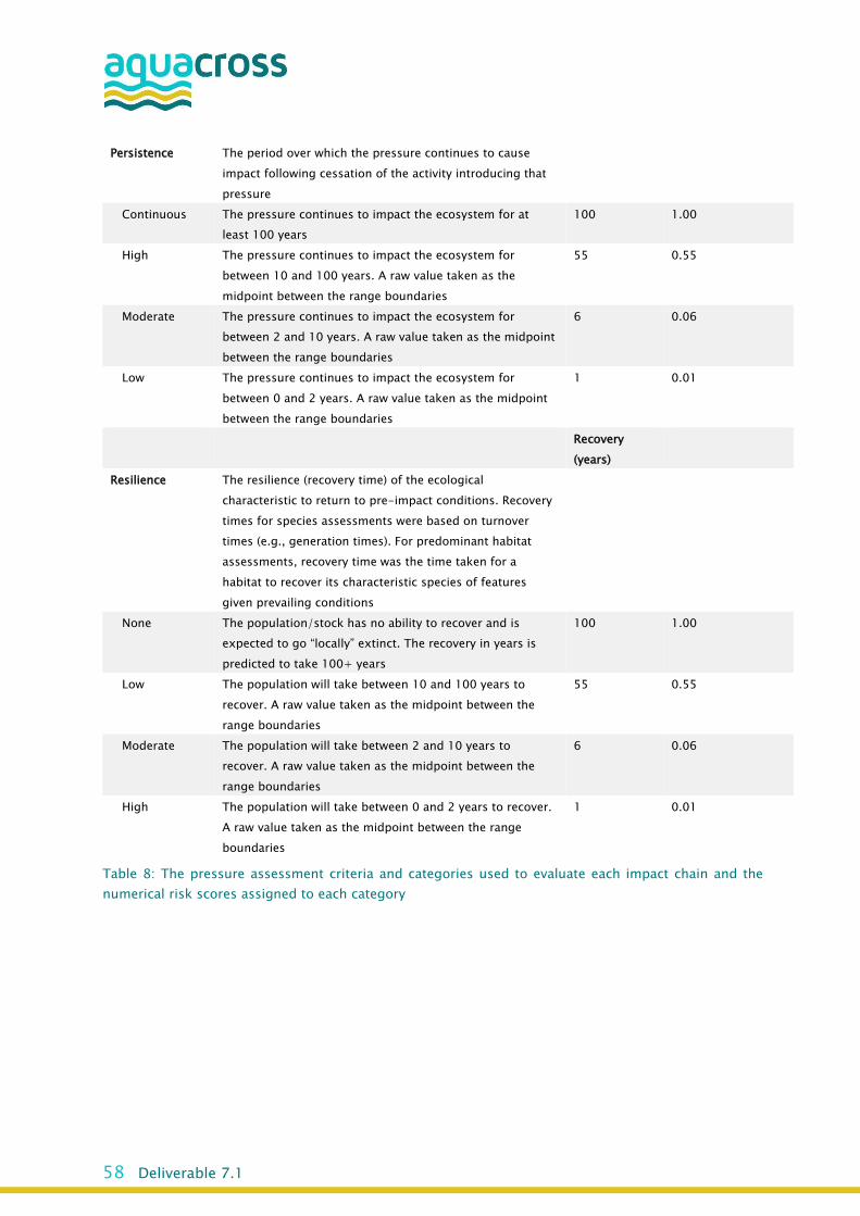
58 Deliverable 7.1
Persistence The period over which the pressure continues to cause
impact following cessation of the activity introducing that
pressure
Continuous The pressure continues to impact the ecosystem for at
least 100 years
100 1.00
High The pressure continues to impact the ecosystem for
between 10 and 100 years. A raw value taken as the
midpoint between the range boundaries
55 0.55
Moderate The pressure continues to impact the ecosystem for
between 2 and 10 years. A raw value taken as the midpoint
between the range boundaries
6 0.06
Low The pressure continues to impact the ecosystem for
between 0 and 2 years. A raw value taken as the midpoint
between the range boundaries
1 0.01
Recovery
(years)
Resilience The resilience (recovery time) of the ecological
characteristic to return to pre-impact conditions. Recovery
times for species assessments were based on turnover
times (e.g., generation times). For predominant habitat
assessments, recovery time was the time taken for a
habitat to recover its characteristic species of features
given prevailing conditions
None The population/stock has no ability to recover and is
expected to go “locally” extinct. The recovery in years is
predicted to take 100+ years
100 1.00
Low The population will take between 10 and 100 years to
recover. A raw value taken as the midpoint between the
range boundaries
55 0.55
Moderate The population will take between 2 and 10 years to
recover. A raw value taken as the midpoint between the
range boundaries
6 0.06
High The population will take between 0 and 2 years to recover.
A raw value taken as the midpoint between the range
boundaries
1 0.01
Table 8: The pressure assessment criteria and categories used to evaluate each impact chain and the
numerical risk scores assigned to each category

59 Deliverable 7.1
9 Outlook
The tools and techniques presented in this report provide an approach that allows (i)
integrating the causal relationships identified in WP4 and WP5 within one workflow, (ii)
including scenario analyses, (iii) integrating stakeholder interactions by setting the targets as
well as during the iteration of the modelling framework to (iv) ultimately achieve a greater
transparency and credibility in the policy context and foreseeing biodiversity conservation and
EBM in the case study areas.
Depending on the aim (qualitative vs. data-driven) and the data availability, the linkage
framework and/or the spatial modelling framework can be applied in the case study areas. As
currently taking place in WP5, the linkages and dependencies within and among the
biodiversity, EF and ESS components need to be explored first. Building on that knowledge, and
if data (quality and quantity) allows, models can be applied to gain more information regarding
the spatial patterns, the uncertainties involved in the data and models, and to assess the impact
of EBM scenarios on biodiversity, EF and ESS as well as in a joint analysis.
One central aim and advantage of the proposed modelling framework is the possibility to
account for uncertainties stemming from the biodiversity side and the ESS side separately as
well as combined within the spatial prioritisation process. This enables to communicate
possible weaknesses and data-deficiencies to stakeholders.
All data and outcomes from the models in the case studies will be available on the Information
Platform36 and shared among project partners. Ad-hoc practical guidance on the proposed
spatial modelling framework will be made available for selected case studies.
36 dataportal.aquacross.eu/

60 Deliverable 7.1
10 References
Allnutt, Thomas F., Timothy R. McClanahan, Serge Andréfouët, Merrill Baker, Erwann
Lagabrielle, Caleb McClennen, Andry J. M. Rakotomanjaka, Tantely F. Tianarisoa, Reg
Watson, and Claire Kremen. 2012. "Comparison of Marine Spatial Planning Methods in
Madagascar Demonstrates Value of Alternative Approaches." PLOS ONE 7 (2):e28969.
doi: 10.1371/journal.pone.0028969.
Álvarez-Romero, Jorge G., Vanessa M. Adams, Robert L. Pressey, Michael Douglas, Allan P.
Dale, Amélie A. Augé, Derek Ball, John Childs, Michael Digby, Rebecca Dobbs, Niilo
Gobius, David Hinchley, Ian Lancaster, Mirjam Maughan, and Ian Perdrisat. 2015.
"Integrated cross-realm planning: A decision-makers' perspective." Biological
Conservation 191:799-808. doi: http://dx.doi.org/10.1016/j.biocon.2015.07.003.
Ardron, Jeff A, Hugh P Possingham, and Carissa J Klein. 2008. "Marxan Good Practices
Handbook, Version 2." Pacific Marine Analysis and Research Association, Victoria, BC,
Canada, 165 pages. www.pacmara.org.
Balbi, S., F. Villa, V. Mojtahed, K. T. Hegetschweiler, and C. Giupponi. 2016. "A spatial
Bayesian network model to assess the benefits of early warning for urban flood risk to
people." Nat. Hazards Earth Syst. Sci. 16 (6):1323-1337. doi: 10.5194/nhess-16-
1323-2016.
Balbi, Stefano, Agustin del Prado, Patricia Gallejones, Chandanathil Pappachan Geevan,
Guillermo Pardo, Elena Pérez-Miñana, Rosa Manrique, Cuitlahuac Hernandez-
Santiago, and Ferdinando Villa. 2015. "Modeling trade-offs among ecosystem services
in agricultural production systems." Environmental Modelling & Software 72:314-326.
doi: https://doi.org/10.1016/j.envsoft.2014.12.017.
Ball, Ian R, Hugh P Possingham, and M Watts. 2009. "Marxan and relatives: software for
spatial conservation prioritisation." Spatial conservation prioritisation: quantitative
methods and computational tools. In: A. Moilanen, Wilson K.A. & Possingham H.P.
(Eds.), Oxford University Press, Oxford, pp. 185-195. :185-195.
Balvanera, Patricia, Andrea B. Pfisterer, Nina Buchmann, Jing-Shen He, Tohru Nakashizuka,
David Raffaelli, and Bernhard Schmid. 2006. "Quantifying the evidence for biodiversity
effects on ecosystem functioning and services." Ecology Letters 9 (10):1146-1156.
doi: 10.1111/j.1461-0248.2006.00963.x.
Balvanera, Patricia, Sandra Quijas, Daniel S. Karp, Neville Ash, Elena M. Bennett, Roel
Boumans, Claire Brown, Kai M. A. Chan, Rebecca Chaplin-Kramer, Benjamin S.
Halpern, Jordi Honey-Rosés, Choong-Ki Kim, Wolfgang Cramer, Maria José Martínez-
Harms, Harold Mooney, Tuyeni Mwampamba, Jeanne Nel, Stephen Polasky, Belinda

61 Deliverable 7.1
Reyers, Joe Roman, Woody Turner, Robert J. Scholes, Heather Tallis, Kirsten Thonicke,
Ferdinando Villa, Matt Walpole, and Ariane Walz. 2017. "Ecosystem Services."39-78.
doi: 10.1007/978-3-319-27288-7_3.
Beger, Maria, Hedley S. Grantham, Robert L. Pressey, Kerrie A. Wilson, Eric L. Peterson, Daniel
Dorfman, Peter J. Mumby, Reinaldo Lourival, Daniel R. Brumbaugh, and Hugh P.
Possingham. 2010. "Conservation planning for connectivity across marine, freshwater,
and terrestrial realms." Biological Conservation 143 (3):565-575. doi:
https://doi.org/10.1016/j.biocon.2009.11.006.
Bohnet, Iris, and Douglas Mark Smith. 2007. "Planning future landscapes in the Wet Tropics
of Australia: A social-ecological framework." Landscape and Urban Planning 80
(1-2):137-152. doi: https://doi.org/10.1016/j.landurbplan.2006.07.001.
Booth, Trevor H., Henry A. Nix, John R. Busby, and Michael F. Hutchinson. 2014. "bioclim: the
first species distribution modelling package, its early applications and relevance to
most current MaxEnt studies." Diversity and Distributions 20 (1):1-9. doi:
10.1111/ddi.12144.
Boria, Robert A., Link E. Olson, Steven M. Goodman, and Robert P. Anderson. 2014. "Spatial
filtering to reduce sampling bias can improve the performance of ecological niche
models." Ecological Modelling 275:73-77. doi:
https://doi.org/10.1016/j.ecolmodel.2013.12.012.
Boumans, Roelof, Joe Roman, Irit Altman, and Les Kaufman. 2015. "The Multiscale Integrated
Model of Ecosystem Services (MIMES): Simulating the interactions of coupled human
and natural systems." Ecosystem Services 12:30-41. doi:
http://dx.doi.org/10.1016/j.ecoser.2015.01.004.
Breiman, Leo. 2001. "Random forests." Machine learning 45 (1):5-32.
Brink, Andreas, Javier Martínez-López, Zoltan Szantoi, Pablo Moreno-Atencia, Andrea Lupi,
Lucy Bastin, and Grégoire Dubois. 2016. "Indicators for Assessing Habitat Values and
Pressures for Protected Areas—An Integrated Habitat and Land Cover Change
Approach for the Udzungwa Mountains National Park in Tanzania." Remote Sensing 8
(10):862.
Brouwer, Roy, Luke Brander, Onno Kuik, Elissaios Papyrakis, and Ian Bateman. 2013. "A
synthesis of approaches to assess and value ecosystem services in the EU in the
context of TEEB." VU University Amsterdam.
Burkhard, Benjamin, and Joachim Maes. 2017. "Mapping Ecosystem Services." Advanced
Books 1:e12837.

62 Deliverable 7.1
Busby, JRꎬ. 1991. "BIOCLIM-a bioclimate analysis and prediction system." Plant protection
quarterly (Australia).
Carlsson-Kanyama, Annika, Karl Henrik Dreborg, H. C. Moll, and Dario Padovan. 2008.
"Participative backcasting: A tool for involving stakeholders in local sustainability
planning." Futures 40 (1):34-46. doi:
https://doi.org/10.1016/j.futures.2007.06.001.
Caudron, Arnaud, Laure Vigier, and Alexis Champigneulle. 2012. "Developing collaborative
research to improve effectiveness in biodiversity conservation practice." Journal of
Applied Ecology 49 (4):753-757. doi: 10.1111/j.1365-2664.2012.02115.x.
Christin, Zachary L., Kenneth J. Bagstad, and Michael A. Verdone. 2016. "A decision
framework for identifying models to estimate forest ecosystem services gains from
restoration." Forest Ecosystems 3 (1):3. doi: 10.1186/s40663-016-0062-y.
Colucci, Erminia. 2007. "“Focus Groups Can Be Fun”: The Use of Activity-Oriented Questions
in Focus Group Discussions." Qualitative Health Research 17 (10):1422-1433. doi:
doi:10.1177/1049732307308129.
Cork, S., G. Peterson, G. Petschel-Held, J. Alcamo, J. Alder, E. Bennett, E. Carr, D. Deane,
G. Nelson, T. Ribeiro, C. Butler, E. Mendiondo, W. Oluoch-Kosura, and M. Zurek.
2005. "Four scenarios. Pages 223-294 in Millennium Ecosystem Assessment .
Ecosystems and human well- being: scenarios. Island Press, Washington, D.C., USA.".
Cormier, Susan M., and Glenn W. Suter II. 2013. "A method for assessing causation of field
exposure-response relationships." Environmental Toxicology and Chemistry 32
(2):272-276. doi: 10.1002/etc.2056.
Costa, Micheli D. P., Hugh P. Possingham, and José Henrique Muelbert. 2016. "Incorporating
early life stages of fishes into estuarine spatial conservation planning." Aquatic
Conservation: Marine and Freshwater Ecosystems 26 (6):1013-1030. doi:
10.1002/aqc.2584.
Costanza, Robert, Ralph d'Arge, Rudolf De Groot, Stephen Farber, Monica Grasso, Bruce
Hannon, Karin Limburg, Shahid Naeem, Robert V O'neill, and Jose Paruelo. 1997. "The
value of the world's ecosystem services and natural capital." Nature 387 (6630):253-
260.
Culhane, Fiona E., Robert A. Briers, Paul Tett, and Teresa F. Fernandes. 2014. "Structural and
functional indices show similar performance in marine ecosystem quality assessment."
Ecological Indicators 43:271-280. doi:
https://doi.org/10.1016/j.ecolind.2014.03.009.

63 Deliverable 7.1
Daily, Gretchen. 1997. Nature's services: societal dependence on natural ecosystems: Island
Press.
de Souza Muñoz, Mauro Enrique, Renato De Giovanni, Marinez Ferreira de Siqueira, Tim
Sutton, Peter Brewer, Ricardo Scachetti Pereira, Dora Ann Lange Canhos, and Vanderlei
Perez Canhos. 2011. "openModeller: a generic approach to species’ potential
distribution modelling." GeoInformatica 15 (1):111-135.
Díaz S, Pascual U, Stenseke M, Martín-López B, Watson RT, Molnár Z, et al. Assessing nature's
contributions to people. Science. 2018;359:270-2. doi: 10.1126/science.aap8826.
Di Cola, Valeria, Olivier Broennimann, Blaise Petitpierre, Frank T. Breiner, Manuela D'Amen,
Christophe Randin, Robin Engler, Julien Pottier, Dorothea Pio, Anne Dubuis, Loic
Pellissier, Rubén G. Mateo, Wim Hordijk, Nicolas Salamin, and Antoine Guisan. 2017.
"ecospat: an R package to support spatial analyses and modeling of species niches
and distributions." Ecography 40 (6):774-787. doi: 10.1111/ecog.02671.
Diniz-Filho, José Alexandre F., Luis Mauricio Bini, Thiago Fernando Rangel, Rafael D. Loyola,
Christian Hof, David Nogués-Bravo, and Miguel B. Araújo. 2009. "Partitioning and
mapping uncertainties in ensembles of forecasts of species turnover under climate
change." Ecography 32 (6):897-906. doi: 10.1111/j.1600-0587.2009.06196.x.
Domisch, Sami, Giuseppe Amatulli, and Walter Jetz. 2015a. "Near-global freshwater-specific
environmental variables for biodiversity analyses in 1 km resolution." Scientific Data
2:150073. doi: 10.1038/sdata.2015.73
http://www.nature.com/articles/sdata201573#supplementary-information.
Domisch, Sami, Miguel B. Araújo, Núria Bonada, Steffen U. Pauls, Sonja C. Jähnig, and Peter
Haase. 2013. "Modelling distribution in European stream macroinvertebrates under
future climates." Global Change Biology 19 (3):752-762. doi: 10.1111/gcb.12107.
Domisch, Sami, Sonja C Jähnig, John P Simaika, Mathias Kuemmerlen, and Stefan Stoll. 2015b.
"Application of species distribution models in stream ecosystems: the challenges of
spatial and temporal scale, environmental predictors and species occurrence data."
Fundamental and Applied Limnology / Archiv für Hydrobiologie. doi:
10.1127/fal/2015/0627.
Domisch, Sami, Adam M. Wilson, and Walter Jetz. 2016. "Model-based integration of
observed and expert-based information for assessing the geographic and
environmental distribution of freshwater species." Ecography 39 (11):1078-1088.
doi: 10.1111/ecog.01925.
Dormann, Carsten F., Stanislaus J. Schymanski, Juliano Cabral, Isabelle Chuine, Catherine
Graham, Florian Hartig, Michael Kearney, Xavier Morin, Christine Römermann, Boris
Schröder, and Alexander Singer. 2012. "Correlation and process in species

64 Deliverable 7.1
distribution models: bridging a dichotomy." Journal of Biogeography 39 (12):2119-
2131. doi: 10.1111/j.1365-2699.2011.02659.x.
Duan, Ren-Yan, Xiao-Quan Kong, Min-Yi Huang, Gan-Lin Wu, and Zhi-Gao Wang. 2015.
"SDMvspecies: a software for creating virtual species for species distribution
modelling." Ecography 38 (1):108-110. doi: 10.1111/ecog.01080.
Dubois, Grégoire, Lucy Bastin, Bastian Bertzky, Andrea Mandrici, Michele Conti, Santiago
Saura, Andrew Cottam, Luca Battistella, Javier Martínez-López, Martino Boni, and
Mariagrazia Graziano. 2016. "Integrating Multiple Spatial Datasets to Assess Protected
Areas: Lessons Learnt from the Digital Observatory for Protected Areas (DOPA)." ISPRS
International Journal of Geo-Information 5 (12):242.
Eitelberg, David A., Jasper van Vliet, Jonathan C. Doelman, Elke Stehfest, and Peter H.
Verburg. 2016. "Demand for biodiversity protection and carbon storage as drivers of
global land change scenarios." Global Environmental Change 40: 101-111.
Elith, Jane, and Catherine H. Graham. 2009. "Do they? How do they? WHY do they differ? On
finding reasons for differing performances of species distribution models." Ecography
32 (1):66-77. doi: 10.1111/j.1600-0587.2008.05505.x.
Elith, Jane, and John R. Leathwick. 2009. "Species Distribution Models: Ecological Explanation
and Prediction Across Space and Time." Annual Review of Ecology, Evolution, and
Systematics 40 (1):677-697. doi: 10.1146/annurev.ecolsys.110308.120159.
Ennis, Marguerite, Geoffrey Hinton, David Naylor, Mike Revow, and Robert Tibshirani. 1998.
"A comparison of statistical learning methods on the GUSTO database." Statistics in
medicine 17 (21):2501-2508.
García-Roselló, Emilio, Cástor Guisande, Jacinto González-Dacosta, Juergen Heine, Patricia
Pelayo-Villamil, Ana Manjarrás-Hernández, Antonio Vaamonde, and Carlos Granado-
Lorencio. 2013. "ModestR: a software tool for managing and analyzing species
distribution map databases." Ecography 36 (11):1202-1207. doi: 10.1111/j.1600-
0587.2013.00374.x.
Gelman, Andrew. 2006. "Multilevel (hierarchical) modeling: what it can and cannot do."
Technometrics 48 (3):432-435.
Gómez, CM, G Delacámara, J Arévalo-Torres, J Barbière, AL Barbosa, B Boteler, F Culhane, M
Daam, MP Gosselin, T Hein, Alejandro Iglesias-Campos, Sonja Jähnig, Manuel Lago,
Simone Langhans, Javier Martínez-López, António Nogueira, Ana Lillebø, Tim
O’Higgins, GerJan Piet, Florian Pletterbauer, Martin Pusch, Peter Reichert, Leonie
Robinson, Josselin Rouillard, and Maja Schlüter. 2016. "The AQUACROSS Innovative
Concept. Deliverable 3.1. European Union’s Horizon 2020 Framework Programme for
Research and Innovation Grant Agreement No. 642317."

65 Deliverable 7.1
Gómez, CM, G Delacámara, S Jähnig, V Mattheiss, S Langhans, S Domisch, V Hermoso, G Piet,
J Martínez-López, and M Lago. 2017. "Developing the AQUACROSS Assessment
Framework. Deliverable 3.2, AQUACROSS, European Union’s Horizon 2020 Framework
Programme for Research and Innovation Grant Agreement No. 642317."
Guisan, Antoine, Anthony Lehmann, Simon Ferrier, Mike Austin, Jacob Mc C. Overton, Richard
Aspinall, and Trevor Hastie. 2006. "Making better biogeographical predictions of
species’ distributions." Journal of Applied Ecology 43 (3):386-392. doi:
10.1111/j.1365-2664.2006.01164.x.
Guo, Qinghua, and Yu Liu. 2010. "ModEco: an integrated software package for ecological
niche modeling." Ecography 33 (4):637-642. doi: 10.1111/j.1600-
0587.2010.06416.x.
Guzy, Michael, Courtland Smith, John Bolte, David Hulse, and Stanley Gregory. 2008. "Policy
research using agent-based modeling to assess future impacts of urban expansion
into farmlands and forests." Ecology and Society 13 (1).
Ha, J, M Eigenraam, G Forbes, W Lewis, and J Chua. 2010. "The Environmental Systems
Modelling Platform (EnSym) to Assess Effects of Land Use Change on Groundwater
Recharge." Proceedings of the 2010 International Environmental Modelling and
Software Society.
Haines-Young, Roy, and Marion Potschin. 2012. "Common international classification of
ecosystem services (CICES, Version 4.1)." European Environment Agency 33.
Harrison, Paula A., Ian P. Holman, George Cojocaru, Kasper Kok, Areti Kontogianni, Marc J.
Metzger, and Marc Gramberger. 2013. "Combining qualitative and quantitative
understanding for exploring cross-sectoral climate change impacts, adaptation and
vulnerability in Europe." Regional Environmental Change 13 (4):761-780. doi:
10.1007/s10113-012-0361-y.
Hein, Lars, Kris van Koppen, Rudolf S. de Groot, and Ekko C. van Ierland. 2006. "Spatial
scales, stakeholders and the valuation of ecosystem services." Ecological Economics
57 (2):209-228. doi: http://dx.doi.org/10.1016/j.ecolecon.2005.04.005.
Hermoso, V., S. Linke, J. Prenda, and H. P. Possingham. 2011. "Addressing longitudinal
connectivity in the systematic conservation planning of fresh waters." Freshwater
Biology 56 (1):57-70. doi: 10.1111/j.1365-2427.2009.02390.x.
Hermoso, Virgilio, Lorenzo Cattarino, Mark J. Kennard, Mathew Watts, and Simon Linke. 2015.
"Catchment zoning for freshwater conservation: refining plans to enhance action on
the ground." Journal of Applied Ecology 52 (4):940-949. doi: 10.1111/1365-
2664.12454.

66 Deliverable 7.1
Hermoso, Virgilio, Ana Filipa Filipe, Pedro Segurado, and Pedro Beja. 2016. "Catchment
zoning to unlock freshwater conservation opportunities in the Iberian Peninsula."
Diversity and Distributions 22 (9):960-969. doi: 10.1111/ddi.12454.
Hijmans, Robert J, and Jane Elith. 2013. "Species distribution modeling with R." R package
version 0.8-11. Available at http://cran.r-
project.org/web/packages/dismo/vignettes/sdm.pdf.
Hijmans, Robert J, Steven Phillips, John Leathwick, Jane Elith, and Maintainer Robert J Hijmans.
2017. "Package ‘dismo’." Circles 9:1.
Hijmans, Robert J., Susan E. Cameron, Juan L. Parra, Peter G. Jones, and Andy Jarvis. 2005.
"Very high resolution interpolated climate surfaces for global land areas."
International Journal of Climatology 25 (15):1965-1978. doi: 10.1002/joc.1276.
Hirzel, A. H., J. Hausser, D. Chessel, and N. Perrin. 2002. "ECOLOGICAL-NICHE FACTOR
ANALYSIS: HOW TO COMPUTE HABITAT-SUITABILITY MAPS WITHOUT ABSENCE DATA?"
Ecology 83 (7):2027-2036. doi: 10.1890/0012-
9658(2002)083[2027:ENFAHT]2.0.CO;2.
Hooper, D. U., F. S. Chapin, J. J. Ewel, A. Hector, P. Inchausti, S. Lavorel, J. H. Lawton, D. M.
Lodge, M. Loreau, S. Naeem, B. Schmid, H. Setälä, A. J. Symstad, J. Vandermeer, and D.
A. Wardle. 2005. "Effects of biodiversity on ecosystem functioning: A consensus of
current knowledge." Ecological Monographs 75 (1):3-35. doi: 10.1890/04-0922.
Hurlbert, Allen H., and Walter Jetz. 2007. "Species richness, hotspots, and the scale
dependence of range maps in ecology and conservation." Proceedings of the National
Academy of Sciences 104 (33):13384-13389. doi: 10.1073/pnas.0704469104.
IPCC. 2000. "Special report on emissions scenarios: a special report of working group III of
the Intergovernmental Panel on Climate Change." Cambridge University Press:
Cambridge, UK.
Jackson, Bethanna, Timothy Pagella, Fergus Sinclair, Barbara Orellana, Alex Henshaw, Brian
Reynolds, Neil McIntyre, Howard Wheater, and Amy Eycott. 2013. "Polyscape: A GIS
mapping framework providing efficient and spatially explicit landscape-scale
valuation of multiple ecosystem services." Landscape and Urban Planning 112:74-88.
doi: https://doi.org/10.1016/j.landurbplan.2012.12.014.
Jarzyna, Marta A., and Walter Jetz. 2016. "Detecting the Multiple Facets of Biodiversity."
Trends in Ecology & Evolution 31 (7):527-538. doi:
http://dx.doi.org/10.1016/j.tree.2016.04.002.
Kakouei, Karan, Jens Kiesel, Jochem Kail, Martin Pusch, and Sonja C. Jähnig. 2017.
"Quantitative hydrological preferences of benthic stream invertebrates in Germany."

67 Deliverable 7.1
Ecological Indicators 79:163-172. doi:
https://doi.org/10.1016/j.ecolind.2017.04.029.
Kakouei, Karan, Domisch, Sami, Kiesel, Jens, Irving S. Katie, Jähnig, Sonja C. and Kail, Jochem.
2018 Projected effects of climate-change-induced flow alterations on stream
macroinvertebrate abundances. Ecology and Evolution. DOI: 10.1002/ece3.3907.
Klein, Carissa Joy, Charles Steinback, Matthew Watts, Astrid J. Scholz, and Hugh P.
Possingham. 2010. "Spatial marine zoning for fisheries and conservation." Frontiers
in Ecology and the Environment 8 (7):349-353. doi: 10.1890/090047.
Knights, Antony M., Rebecca S. Koss, and Leonie A. Robinson. 2013. "Identifying common
pressure pathways from a complex network of human activities to support
ecosystem-based management." Ecological Applications 23 (4):755-765. doi:
10.1890/12-1137.1.
Knights, Antony M., Gerjan J. Piet, Ruud H. Jongbloed, Jacqueline E. Tamis, Lydia White, Ekin
Akoglu, Laura Boicenco, Tanya Churilova, Olga Kryvenko, Vivi Fleming-Lehtinen, Juha-
Markku Leppanen, Bella S. Galil, Freya Goodsir, Menachem Goren, Piotr Margonski,
Snejana Moncheva, Temel Oguz, K. Nadia Papadopoulou, Outi Setälä, Chris J. Smith,
Kremena Stefanova, Florin Timofte, and Leonie A. Robinson. 2015. "An exposure-
effect approach for evaluating ecosystem-wide risks from human activities." ICES
Journal of Marine Science 72 (3):1105-1115. doi: 10.1093/icesjms/fsu245.
Koch, Evamaria W., Edward B. Barbier, Brian R. Silliman, Denise J. Reed, Gerardo M. E. Perillo,
Sally D. Hacker, Elise F. Granek, Jurgenne H. Primavera, Nyawira Muthiga, Stephen
Polasky, Benjamin S. Halpern, Christopher J. Kennedy, Carrie V. Kappel, and Eric
Wolanski. 2009. "Non-linearity in ecosystem services: temporal and spatial variability
in coastal protection." Frontiers in Ecology and the Environment 7 (1):29-37. doi:
10.1890/080126.
Kok, Kasper, Reinette Oonsie Biggs, and Monika Zurek. 2007. "Methods for developing
multiscale participatory scenarios: insights from southern Africa and Europe." Ecology
and Society 12 (1).
Komossa, Franziska, Emma H. van der Zanden, Catharina JE Schulp, and Peter H. Verburg.
2018. "Mapping landscape potential for outdoor recreation using different
archetypical recreation user groups in the European Union." Ecological Indicators 85:
105-116.
Kumazawa, Terukazu, Osamu Saito, Kouji Kozaki, Takanori Matsui, and Riichiro Mizoguchi.
2009. "Toward knowledge structuring of sustainability science based on ontology
engineering." Sustainability Science 4 (1):99. doi: 10.1007/s11625-008-0063-z.

68 Deliverable 7.1
Kwakkel, Jan H., and Erik Pruyt. 2013. "Exploratory Modeling and Analysis, an approach for
model-based foresight under deep uncertainty." Technological Forecasting and Social
Change 80 (3):419-431. doi: https://doi.org/10.1016/j.techfore.2012.10.005.
Landsberg, F, S Ozment, M Stickler, N Henninger, J Treweek, O Venn, and G Mock. 2011.
"Ecosystem services review for impact assessment." World Business Council for
Sustainable Development and World Resources Institute. Available at http://www. wri.
org/publication/ecosystem-services-review-for-impact-assessment.
Langhans, Simone D., Jörn Gessner, Virgilio Hermoso, and Christian Wolter. 2016. "Coupling
systematic planning and expert judgement enhances the efficiency of river
restoration." Science of The Total Environment 560-561:266-273. doi:
https://doi.org/10.1016/j.scitotenv.2016.03.232.
Langhans, Simone D., Virgilio Hermoso, Simon Linke, Stuart E. Bunn, and Hugh P.
Possingham. 2014. "Cost-effective river rehabilitation planning: Optimizing
for morphological benefits at large spatial scales." Journal of Environmental
Management 132:296-303. doi: https://doi.org/10.1016/j.jenvman.2013.11.021.
Latimer, Andrew M., Shanshan Wu, Alan E. Gelfand, and John A. Silander. 2006. "Building
Statistical Models To Analyze Species Distributions." Ecological Applications 16
(1):33-50. doi: 10.1890/04-0609.
Lauzeral, Christine, Gaël Grenouillet, and Sébastien Brosse. 2015. "The iterative ensemble
modelling approach increases the accuracy of fish distribution models." Ecography 38
(2):213-220.
Lehner, B., K. Verdin, and A. Jarvis. 2008. "Eos, Transactions, American Geophysical Union
Volume 89, Number 10, 4 March 2008." Eos, Transactions American Geophysical
Union 89 (10):n/a-n/a. doi: 10.1029/eost2008EO10.
Leroy, Boris, Christine N. Meynard, Céline Bellard, and Franck Courchamp. 2016.
"virtualspecies, an R package to generate virtual species distributions." Ecography 39
(6):599-607. doi: 10.1111/ecog.01388.
Levin, Noam, Tessa Mazor, Eran Brokovich, Pierre-Elie Jablon, and Salit Kark. 2015.
"Sensitivity analysis of conservation targets in systematic conservation planning."
Ecological Applications 25 (7):1997-2010. doi: 10.1890/14-1464.1.
Linke, Simon, Mark J. Kennard, Virgilio Hermoso, Julian D. Olden, Janet Stein, and Bradley J.
Pusey. 2012. "Merging connectivity rules and large-scale condition assessment
improves conservation adequacy in river systems." Journal of Applied Ecology 49
(5):1036-1045. doi: 10.1111/j.1365-2664.2012.02177.x.

69 Deliverable 7.1
Liu, Jianguo, Wu Yang, and Shuxin Li. 2016. "Framing ecosystem services in the telecoupled
Anthropocene." Frontiers in Ecology and the Environment 14 (1):27-36. doi:
10.1002/16-0188.1.
Loreau, M., S. Naeem, P. Inchausti, J. Bengtsson, J. P. Grime, A. Hector, D. U. Hooper, M. A.
Huston, D. Raffaelli, B. Schmid, D. Tilman, and D. A. Wardle. 2001. "Biodiversity and
Ecosystem Functioning: Current Knowledge and Future Challenges." Science 294
(5543):804-808. doi: 10.1126/science.1064088.
Maes, Joachim, Benis Egoh, Louise Willemen, Camino Liquete, Petteri Vihervaara, Jan Philipp
Schägner, Bruna Grizzetti, Evangelia G. Drakou, Alessandra La Notte, Grazia Zulian,
Faycal Bouraoui, Maria Luisa Paracchini, Leon Braat, and Giovanni Bidoglio. 2012.
"Mapping ecosystem services for policy support and decision making in the European
Union." Ecosystem Services 1 (1):31-39. doi:
http://dx.doi.org/10.1016/j.ecoser.2012.06.004.
Maes, Joachim, Camino Liquete, Anne Teller, Markus Erhard, Maria Luisa Paracchini, José I.
Barredo, Bruna Grizzetti, Ana Cardoso, Francesca Somma, Jan-Erik Petersen, Andrus
Meiner, Eva Royo Gelabert, Nihat Zal, Peter Kristensen, Annemarie Bastrup-Birk,
Katarzyna Biala, Chiara Piroddi, Benis Egoh, Patrick Degeorges, Christel Fiorina,
Fernando Santos-Martín, Vytautas Naruševičius, Jan Verboven, Henrique M. Pereira,
Jan Bengtsson, Kremena Gocheva, Cristina Marta-Pedroso, Tord Snäll, Christine
Estreguil, Jesus San-Miguel-Ayanz, Marta Pérez-Soba, Adrienne Grêt-Regamey, Ana I.
Lillebø, Dania Abdul Malak, Sophie Condé, Jon Moen, Bálint Czúcz, Evangelia G.
Drakou, Grazia Zulian, and Carlo Lavalle. 2016. "An indicator framework for assessing
ecosystem services in support of the EU Biodiversity Strategy to 2020." Ecosystem
Services 17:14-23. doi: https://doi.org/10.1016/j.ecoser.2015.10.023.
Maes, Joachim, Anne Teller, Markus Erhard, C Liquete, L Braat, P Berry, B Egoh, P Puydarrieux,
C Fiorina, and F Santos. 2013. "Mapping and Assessment of Ecosystems and their
Services. Indicators for Ecosystem Assessments under Action 5 of the EU Biodiversity
Strategy to 2020.” " Publications Office of the European Union, Luxembourg.
doi:10.2779/75203.
Martínez-Fernández, Julia, Miguel-Angel Esteve-Selma, Jose-Miguel Martínez-Paz, María-
Francisca Carreño, Javier Martínez-López, Francisco Robledano, and Pablo Farinós.
2014. "Chapter 11 - Trade-Offs Between Biodiversity Conservation and Nutrients
Removal in Wetlands of Arid Intensive Agricultural Basins: The Mar Menor Case,
Spain." In Developments in Environmental Modelling, edited by Ni-Bin Chang Sven Erik
Jørgensen and Xu Fu-Liu, 275-310. Elsevier.
Martínez-López, J., M. F. Carreño, J. Martínez-Fernández, and M. A. Esteve. 2014a. "Wetland
and landscape indices for assessing the condition of semiarid Mediterranean saline
wetlands under agricultural hydrological pressures." Ecological Indicators 36:400-
408. doi: https://doi.org/10.1016/j.ecolind.2013.08.007.

70 Deliverable 7.1
Martínez-López, J., M. F. Carreño, J. A. Palazón-Ferrando, J. Martínez-Fernández, and M. A.
Esteve. 2014b. "Remote sensing of plant communities as a tool for assessing the
condition of semiarid Mediterranean saline wetlands in agricultural catchments."
International Journal of Applied Earth Observation and Geoinformation 26:193-204.
doi: https://doi.org/10.1016/j.jag.2013.07.005.
Martínez-López, Javier, Bastian Bertzky, Francisco Bonet-García, Lucy Bastin, and Grégoire
Dubois. 2016. "Biophysical Characterization of Protected Areas Globally through
Optimized Image Segmentation and Classification." Remote Sensing 8 (9):780.
Martínez-López, Javier, Julia Martínez-Fernández, Babak Naimi, María F. Carreño, and Miguel
A. Esteve. 2015. "An open-source spatio-dynamic wetland model of plant community
responses to hydrological pressures." Ecological Modelling 306:326-333. doi:
https://doi.org/10.1016/j.ecolmodel.2014.11.024.
Menzel, Susanne, and Jack Teng. 2010. "Ecosystem Services as a Stakeholder-Driven Concept
for Conservation Science." Conservation Biology 24 (3):907-909.
Mills, Morena, Vanessa M. Adams, Robert L. Pressey, Natalie C. Ban, and Stacy D. Jupiter.
2012. "Where do national and local conservation actions meet? Simulating the
expansion of ad hoc and systematic approaches to conservation into the future in
Fiji." Conservation Letters 5 (5):387-398. doi: 10.1111/j.1755-263X.2012.00258.x.
Moilanen, Atte, H Kujala, and JR Leathwick. 2009. "The Zonation framework and software for
conservation prioritization." Spatial conservation prioritization:196-210.
Mulligan, Mark. 2015. "Waterworld and Co $ ting Nature: Web-Based Policy Support Systems."
2015 AAAS Annual Meeting (12-16 February 2015).
Naimi, B. 2015. usdm: Uncertainty analysis for species distribution models, R package version
1.1-12.
Naimi, Babak, and Miguel B. Araújo. 2016. "sdm: a reproducible and extensible R platform for
species distribution modelling." Ecography 39 (4):368-375. doi:
10.1111/ecog.01881.
Nenzén, Hedvig K., Rebecca M. Swab, David A. Keith, and Miguel B. Araújo. 2012.
"demoniche - an R-package for simulating spatially-explicit population dynamics."
Ecography 35 (7):577-580. doi: 10.1111/j.1600-0587.2012.07378.x.
Niemeijer, David, and Rudolf S. de Groot. 2008. "Framing environmental indicators: moving
from causal chains to causal networks." Environment, Development and Sustainability
10 (1):89-106. doi: 10.1007/s10668-006-9040-9.
Nogueira, António, Ana Lillebø, Heliana Teixeira, Michiel Daam, L. Robinson, F. Culhane,
Gonzalo Delacámara, Carlos M Gómez, Marta Arenas, Simone D. Langhans, J.

71 Deliverable 7.1
Martínez-López, A. Funk, P. Reichert, N. Schuwirth, P. Vermeiren, and V. Mattheiß.
2016. Guidance on methods and tools for the assesment of causal flow indicators
between diodiversity, ecoystem functions and ecosystem service in the aquatic
environment: Deliverable 5.1, European Union’s Horizon 2020 Framework Programme
for Research and Innovation Grant Agreement No. 642317.: European Union.
Norton, Susan B, Susan M Cormier, and Glenn W Suter II. 2014. Ecological causal assessment:
CRC Press.
Olden, Julian D. , Joshua J. Lawler, and N. LeRoy Poff. 2008. "Machine Learning Methods
Without Tears: A Primer for Ecologists." The Quarterly Review of Biology 83 (2):171-
193. doi: 10.1086/587826.
Ovaskainen, Otso, and Janne Soininen. 2011. "Making more out of sparse data: hierarchical
modeling of species communities." Ecology 92 (2):289-295. doi: 10.1890/10-
1251.1.
Palomo, Ignacio, Berta Martín-López, Cesar López-Santiago, and Carlos Montes. 2011.
"Participatory scenario planning for protected areas management under the ecosystem
services framework: the Doñana social-ecological system in southwestern Spain."
Ecology and Society 16 (1).
Pearson, Richard G. 2007. "Species’ distribution modeling for conservation educators and
practitioners." Synthesis. American Museum of Natural History 1:1-50.
Peh, Kelvin S. H., Andrew Balmford, Richard B. Bradbury, Claire Brown, Stuart H. M. Butchart,
Francine M. R. Hughes, Alison Stattersfield, David H. L. Thomas, Matt Walpole, Julian
Bayliss, David Gowing, Julia P. G. Jones, Simon L. Lewis, Mark Mulligan, Bhopal
Pandeya, Charlie Stratford, Julian R. Thompson, Kerry Turner, Bhaskar Vira, Simon
Willcock, and Jennifer C. Birch. 2013. "TESSA: A toolkit for rapid assessment of
ecosystem services at sites of biodiversity conservation importance." Ecosystem
Services 5:51-57. doi: https://doi.org/10.1016/j.ecoser.2013.06.003.
Phillips, Steven J., Robert P. Anderson, Miroslav Dudík, Robert E. Schapire, and Mary E. Blair.
2017. "Opening the black box: an open-source release of Maxent." Ecography:n/a-
n/a. doi: 10.1111/ecog.03049.
Phillips, Steven J., Robert P. Anderson, and Robert E. Schapire. 2006. "Maximum entropy
modeling of species geographic distributions." Ecological Modelling 190 (3-4):231-
259. doi: https://doi.org/10.1016/j.ecolmodel.2005.03.026.
Piet, Gerjan J., Ruud H. Jongbloed, Antony M. Knights, Jacqueline E. Tamis, Anneke J.
Paijmans, Marieken T. van der Sluis, Pepijn de Vries, and Leonie A. Robinson. 2015.
"Evaluation of ecosystem-based marine management strategies based on risk

72 Deliverable 7.1
assessment." Biological Conservation 186:158-166. doi:
https://doi.org/10.1016/j.biocon.2015.03.011.
Pletterbauer, Florian, Andrea Funk, Thomas Hein, Leonie Robinson, Fiona Culhane, Gonzalo
Delacamara, Carlos M Gomez, Helen Klimmek, GJ Piet, JE Tamis, M. Schlüter, and R.
Martin. 2016. Drivers of change and pressures on aquatic ecosystems: AQUACROSS
Deliverable 4.1, European Union’s Horizon 2020 Framework Programme for Research
and Innovation Grant Agreement No. 642317. European Union.
Plummer, Martyn, A. Stukalov, and M. Denwood. 2016. "Rjags: Bayesian Graphical Models
using MCMC." R package version 4-6 http://mcmc-jags.sourceforge.net.
Pollock, Laura J., Reid Tingley, William K. Morris, Nick Golding, Robert B. O'Hara, Kirsten M.
Parris, Peter A. Vesk, Michael A. McCarthy, and Jana McPherson. 2014. "Understanding
co-occurrence by modelling species simultaneously with a Joint Species Distribution
Model (JSDM)." Methods in Ecology and Evolution 5 (5):397-406. doi: 10.1111/2041-
210x.12180.
Qiao, Huijie, A. Townsend Peterson, Lindsay P. Campbell, Jorge Soberón, Liqiang Ji, and Luis
E. Escobar. 2016. "NicheA: creating virtual species and ecological niches in
multivariate environmental scenarios." Ecography 39 (8):805-813. doi:
10.1111/ecog.01961.
Qiao, Huijie, Jorge Soberón, and Andrew Townsend Peterson. 2015. "No silver bullets in
correlative ecological niche modelling: insights from testing among many potential
algorithms for niche estimation." Methods in Ecology and Evolution 6 (10):1126-
1136. doi: 10.1111/2041-210X.12397.
Robards, Martin D., Michael L. Schoon, Chanda L. Meek, and Nathan L. Engle. 2011. "The
importance of social drivers in the resilient provision of ecosystem services." Global
Environmental Change 21 (2):522-529. doi:
http://dx.doi.org/10.1016/j.gloenvcha.2010.12.004.
Robinson, L.A., F.E. Culhane, C. Baulcomb, H. Bloomfield, A. Boehnke-Henrichs, P. Breen, F.
Goodsir, S.S. Hussain, A.M. Knights, G.J. Piet, J. Raakjaer, J. van Tatenhove, and C.L.J.
Frid. 2014. "Towards delivering ecosystem-based marine management: The ODEMM
Approach. Deliverable 17, EC FP7 Project (244273) ‘Options for Delivering Ecosystem-
based Marine Management’. University of Liverpool. ISBN: 978-0-906370-89-6 : 96
pp.".
Robinson, L.A., A.M. Knights, F.E. Culhane, and A.M. Knights. 2013. "ODEMM pressure
assessment userguide V.2., ODEMM Guidance Document Series No. 4. University of
Liverpool, Liverpool pg. 15 pp."

73 Deliverable 7.1
Royle, J. Andrew, James D. Nichols, and Marc Kéry. 2005. "Modelling occurrence and
abundance of species when detection is imperfect." Oikos 110 (2):353-359. doi:
10.1111/j.0030-1299.2005.13534.x.
Ruiz-Frau, Ana, Hugh P. Possingham, Gareth Edwards-Jones, Carissa J. Klein, Daniel Segan,
and Michel J. Kaiser. 2015. "A multidisciplinary approach in the design of marine
protected areas: Integration of science and stakeholder based methods." Ocean &
Coastal Management 103:86-93. doi:
https://doi.org/10.1016/j.ocecoaman.2014.11.012.
Sbrocco, Elizabeth J., and Paul H. Barber. 2013. "MARSPEC: ocean climate layers for marine
spatial ecology." Ecology 94 (4):979-979. doi: 10.1890/12-1358.1.
Scachetti-Pereira, R. 2002. "DesktopGarp: a software package for biodiversity and ecologic
research." University of Kansas Biodiversity Research Center, EU< http://www. nhm.
ku. edu/desktopgarp/>(consultado 3 marzo 2014).[Links].
Schmidt-Kloiber, Astrid, and Daniel Hering. 2015. "www. freshwaterecology. info-An online
tool that unifies, standardises and codifies more than 20,000 European freshwater
organisms and their ecological preferences." Ecological Indicators 53:271-282.
Schmiing, Mara, Hugo Diogo, Ricardo Serrão Santos, and Pedro Afonso. 2015. "Marine
conservation of multispecies and multi-use areas with various conservation objectives
and targets." ICES Journal of Marine Science 72 (3):851-862.
Sharps, Katrina, Dario Masante, Amy Thomas, Bethanna Jackson, John Redhead, Linda May,
Havard Prosser, Bernard Cosby, Bridget Emmett, and Laurence Jones. 2017.
"Comparing strengths and weaknesses of three ecosystem services modelling tools in
a diverse UK river catchment." Science of The Total Environment 584-585:118-130.
doi: https://doi.org/10.1016/j.scitotenv.2016.12.160.
Sherrouse, Benson C., Jessica M. Clement, and Darius J. Semmens. 2011. "A GIS application
for assessing, mapping, and quantifying the social values of ecosystem services."
Applied Geography 31 (2):748-760. doi:
https://doi.org/10.1016/j.apgeog.2010.08.002.
Smith, Christopher J., Konstantia-Nadia Papadopoulou, Steve Barnard, Krysia Mazik, Michael
Elliott, Joana Patrício, Oihana Solaun, Sally Little, Natasha Bhatia, and Angel Borja.
2016. "Managing the Marine Environment, Conceptual Models and Assessment
Considerations for the European Marine Strategy Framework Directive." Frontiers in
Marine Science 3 (144). doi: 10.3389/fmars.2016.00144.
Stehfest, Elke, Detlef van Vuuren, L Bouwman, and Tom Kram. 2014. Integrated assessment
of global environmental change with IMAGE 3.0: Model description and policy
applications: Netherlands Environmental Assessment Agency (PBL).

74 Deliverable 7.1
Stockwell, David R. B., and A. Townsend Peterson. 2002. "Effects of sample size on accuracy
of species distribution models." Ecological Modelling 148 (1):1-13. doi:
https://doi.org/10.1016/S0304-3800(01)00388-X.
Suter, Glenn W., Susan B. Norton, and Susan M. Cormier. 2002. "A methodology for inferring
the causes of observed impairments in aquatic ecosystems." Environmental
Toxicology and Chemistry 21 (6):1101-1111. doi: 10.1002/etc.5620210602.
Tallis, HT, T Ricketts, AD Guerry, SA Wood, R Sharp, E Nelson, D Ennaanay, S Wolny, N
Olwero, and K Vigerstol. 2013. "InVEST 2.5. 3 User’s Guide. The natural capital
project." Stanford, Available at http://ncp‐dev. stanford. edu/~ dataportal/invest‐
releases/documentation/current_release/, last accessed February 22:2015.
R Development Core Team (2017). R: A language and environment for statistical computing.
R Foundation for Statistical Computing, Vienna, Austria. ISBN 3-900051-07-0, URL
http://www.R-project.org.
Team, Stan Development. 2016. "RStan: the R interface to Stan. R package version 2.14.1.
http://mc-stan.org."
Thuiller, Wilfried, Bruno Lafourcade, Robin Engler, and Miguel B. Araújo. 2009. "BIOMOD - a
platform for ensemble forecasting of species distributions." Ecography 32 (3):369-
373. doi: 10.1111/j.1600-0587.2008.05742.x.
Troy, Austin, and Matthew A. Wilson. 2006. "Mapping ecosystem services: Practical
challenges and opportunities in linking GIS and value transfer." Ecological Economics
60 (2):435-449. doi: https://doi.org/10.1016/j.ecolecon.2006.04.007.
Tulloch, Vivitskaia J., Hugh P. Possingham, Stacy D. Jupiter, Chris Roelfsema, Ayesha I. T.
Tulloch, and Carissa J. Klein. 2013. "Incorporating uncertainty associated with habitat
data in marine reserve design." Biological Conservation 162:41-51. doi:
https://doi.org/10.1016/j.biocon.2013.03.003.
van Zanten, Boris T., Derek B. Van Berkel, Ross K. Meentemeyer, Jordan W. Smith, Koen F.
Tieskens, and Peter H. Verburg. 2016. "Continental-scale quantification of landscape
values using social media data." Proceedings of the National Academy of Sciences
113, no. 46: 12974-12979.
Vieilledent, Ghislain , Cory Merow, Jérôme Guélat, Andrew M. Latimer, Marc Kéry, Alan E.
Gelfand, Adam M. Wilson, Frédéric Mortier, and John A. Silander Jr. 2014. "hSDM:
hierarchical Bayesian species distribution models. URL http://cran.r-
project.org/web/packages/hSDM/index.html."

75 Deliverable 7.1
Villa, F, S Balbi, IN Athanasiadis, and C Caracciolo. 2017. "Semantics for interoperability of
distributed data and models: Foundations for better-connected information."
F1000Research 6 (686).
Villa, Ferdinando, Kenneth J. Bagstad, Brian Voigt, Gary W. Johnson, Rosimeiry Portela,
Miroslav Honzák, and David Batker. 2014. "A Methodology for Adaptable and Robust
Ecosystem Services Assessment." PLOS ONE 9 (3):e91001. doi:
10.1371/journal.pone.0091001.
Villa, Ferdinando, Leonardo Tunesi, and Tundi Agardy. 2002. "Zoning Marine Protected Areas
through Spatial Multiple‐Criteria Analysis: the Case of the Asinara Island National
Marine Reserve of Italy." Conservation Biology 16 (2):515-526. doi:
doi:10.1046/j.1523-1739.2002.00425.x.
Waring, Timothy M, Michelle Ann Kline, Jeremy S Brooks, Sandra H Goff, John Gowdy, Marco A
Janssen, Paul E Smaldino, and Jennifer Jacquet. 2015. "A multilevel evolutionary
framework for sustainability analysis." Ecology and Society 20 (2):34.
Warren, Dan L., Richard E. Glor, and Michael Turelli. 2010. "ENMTools: a toolbox for
comparative studies of environmental niche models." Ecography 33 (3):607-611. doi:
10.1111/j.1600-0587.2009.06142.x.
Warton, David I., F. Guillaume Blanchet, Robert B. O’Hara, Otso Ovaskainen, Sara Taskinen,
Steven C. Walker, and Francis K. C. Hui. 2015. "So Many Variables: Joint Modeling in
Community Ecology." Trends in Ecology & Evolution 30 (12):766-779. doi:
https://doi.org/10.1016/j.tree.2015.09.007.
Watts, Matthew E., Ian R. Ball, Romola S. Stewart, Carissa J. Klein, Kerrie Wilson, Charles
Steinback, Reinaldo Lourival, Lindsay Kircher, and Hugh P. Possingham. 2009.
"Marxan with Zones: Software for optimal conservation based land- and sea-use
zoning." Environmental Modelling & Software 24 (12):1513-1521. doi:
http://dx.doi.org/10.1016/j.envsoft.2009.06.005.
Wollenberg, Eva, David Edmunds, and Louise Buck. 2000. "Using scenarios to make decisions
about the future: anticipatory learning for the adaptive co-management of community
forests." Landscape and Urban Planning 47 (1-2):65-77. doi:
https://doi.org/10.1016/S0169-2046(99)00071-7.
Worm, Boris, Edward B. Barbier, Nicola Beaumont, J. Emmett Duffy, Carl Folke, Benjamin S.
Halpern, Jeremy B. C. Jackson, Heike K. Lotze, Fiorenza Micheli, Stephen R. Palumbi,
Enric Sala, Kimberley A. Selkoe, John J. Stachowicz, and Reg Watson. 2006. "Impacts of
Biodiversity Loss on Ocean Ecosystem Services." Science 314 (5800):787-790. doi:
10.1126/science.1132294.

76 Deliverable 7.1
Yeung, Saiwing, and Thomas L. Griffiths. 2015. "Identifying expectations about the strength
of causal relationships." Cognitive Psychology 76:1-29. doi:
https://doi.org/10.1016/j.cogpsych.2014.11.001.
Zulian, G, C Polce, and J Maes. 2014. "ESTIMAP: a GIS-based model to map ecosystem
services in the European union." Annali di Botanica 4:1-7. doi: 10.4462/annbotrm-
11807.

77 Deliverable 7.1
AQUACROSS PARTNERS
Ecologic Institute (ECOLOGIC) | Germany
Leibniz Institute of Freshwater Ecology and Inland
Fisheries (FVB-IGB) | Germany
Intergovernmental Oceanographic Commission
of the United Nations Educational, Scientific and
Cultural Organization (IOC-UNESCO) | France
Wageningen Marine Research (WMR) | Netherlands
University of Natural Resources & Life Sciences,
Institute of Hydrobiology and Aquatic Ecosystem Management (BOKU) |
Austria
Fundación IMDEA Agua (IMDEA) | Spain
Universidade de Aveiro (UAVR) | Portugal
ACTeon - Innovation, Policy, Environment
(ACTeon) | France
University of Liverpool (ULIV) | United Kingdom
University College Cork, National University
of Ireland (UCC) | Ireland
Royal Belgian Institute of Natural Sciences
(RBINS) | Belgium
Stockholm University, Stockholm Resilience
Centre (SU-SRC) | Sweden
Danube Delta National Institute for Research
& Development (INCDDD) | Romania
Eawag - Swiss Federal Institute of Aquatic
Science and Technology (EAWAG) | Switzerland
International Union for Conservation of Nature
(IUCN) | Belgium
BC3 Basque Centre for Climate Change
(BC3) | Spain
Contact Coordinator
Duration Website
LinkedIn ResearchGate
Dr. Manuel Lago, Ecologic Institute 1 June 2015 to 30 November 2018 http://aquacross.eu/
@AquaBiodiv
www.linkedin.com/groups/AQUACROSS-8355424/about https://goo.gl/IcdtZC