modelling and simulation of the closed injection
TRANSCRIPT

Modelling and Simulation of the Closed Injection
Pultrusion Process
Zur Erlangung des akademischen Grades
Doktor der Ingenieurwissenschaften
der Fakultät für Maschinenbau
Karlsruher Institut für Technologie (KIT)
genehmigte
Dissertation
von
M.Sc. Renato Menezes Bezerra
Tag der mündlichen Prüfung: 24.10.2017
Hauptreferent: Prof. Dr.-Ing. Frank Henning
Korreferent: Prof. Dr.-Ing. Klaus Drechsler


Preamble I
Preamble
This Ph.D. thesis was undertaken during my engagement as a research employee at the
Fraunhofer Society. During this period, I have had the pleasure to work at the Institute for
Chemical Technology (ICT) in Pfinztal, Germany, later on at the project group Functional
Lightweight Design (FIL) and at the Fraunhofer Research Institution for Casting, Composite
and Processing Technology (IGCV) in Augsburg, Germany.
I would like to thank Prof. Dr.-Ing. Frank Henning for supervising my thesis and believing in
the quality of my research work. I also thank Prof. Dr.-Ing. Klaus Drechsler for reviewing my
work as a second supervisor and giving valuable insight.
Part of this thesis was conducted within the project PulForm funded by the German Federal
Ministry of Education and Research (BMBF) (funding number 02PJ2035). Part of the
experimental work was conducted within the general start-up activities of the project group
FIL, funded by the Region of Bavaria, the City of Augsburg, BMBF and the European Union. I
would like to acknowledge the financial support provided.
For the technical support, discussions and teamwork I would like to thank my colleagues
Ingo Anschütz, Frederik Wilhelm, Sebastian Strauß and Alexander Chaloupka. I also
appreciate the efforts of Dr. Iman Taha and Dr. John Puentes in reviewing this thesis and
giving valuable input. A special thanks to Lazarula Chatzigeorgiou for making it possible to
explore this topic at IGCV and for providing a flexible work environment. Many thanks also to
all colleagues whom I may not have remembered here, but were helpful in many direct and
indirect ways.
I would also like to thank my parents-in-law Yeda and Marcos for their continuous support
and for their interest in my work. Finally, and most importantly, I would like to thank my wife
Melissa for her endless support and patience and my daughters Luisa and Helena for
clearing my mind from work every now and then, and pointing out the really important things
in life. You are the joy of my life.
Augsburg, August 2017 Renato Menezes Bezerra

II Abstract
Abstract
Pultrusion is a mature processing technology for producing fiber reinforced composite
profiles. The process is characterized by a relatively high level of automation at low
investment and production costs in comparison to most other processing methods for
composite parts. In a standard open bath pultrusion setup, an open tank filled with liquid
resin is employed to wet the fiber reinforcement materials. Current technology and regulatory
developments have started a trend that is expected to radically change the pultrusion
industry state of the art in the long term. Examples include the tightening of working place
regulations, the introduction of new resins of relatively short pot life (e.g. polyurethanes) to
the pultrusion market, as well as the requirements of new applications with higher product
quality demands (e.g. in the automotive sector). The design of pultrusion molds with
integrated or attached cavities into which the resin is injected and thus impregnates the fiber
reinforcements immediately before curing is foreseen to replace the open bath method.
In this thesis, simulation techniques are employed to get insight and a better understanding
for the physical processes taking place within pultrusion molds with closed resin injection and
impregnation: resin flow through the fiber stack while this is being compacted, heat transfer
between material and mold, and resin curing reaction (coupled with changes in material state
and release of exothermic reaction heat). To investigate these phenomena, material
parameters of resin (curing kinetics and development of viscosity throughout curing) and
fiber reinforcement (compressibility and permeability) are experimentally determined. The
material parameters, a geometrical model of the pultrusion mold and suitable boundary
conditions are used as the input for the numerical simulation conducted within a
Computational Fluid Dynamics commercial software and complemented by an in-house
Finite Difference code. The simulation calculates pressure, temperature, viscosity and
degree of cure distributions within the mold cavity. Simulation results are compared to
experimental processing conditions to validate the simulation model. Design details and
process parameters are then varied and their impact on processing conditions is analyzed.
The simulation results have shown that the holistic approach pursued in this work, i.e. the
coupling of thermo-chemical and flow models is needed for obtaining accurate predictions for
the case of a fast reacting resin system. On the other hand, an expansion of the simulation
models to account for mold body deformation would be necessary to improve the pressure
rise prediction. Furthermore, depending on the cavity design, resin system and processing
conditions, transient simulations would be needed for a better prediction and evaluation of
process stability.

Kurzfassung III
Kurzfassung
Pultrusion ist eine etablierte Herstellungstechnik für die Produktion faserverstärkter
Kunststoffprofile. Der Prozess ist durch einen relativ hohen Automatisierungsgrad und
geringe Investitions- und Betriebskosten im Vergleich zu den meisten anderen
Herstellungstechniken für Faserverbundbauteile gekennzeichnet. Als Standard-Variante wird
ein offener, mit flüssigem Harz gefüllten Behälter für die Tränkung der
Faserverstärkungsmaterialien eingesetzt. Die Verschärfung von Gesetzen zum Schutz von
Mitarbeitern am Arbeitsplatz, die Einführung neuer Harzsysteme mit kurzer Topfzeit (z.B.
Polyurethane), sowie gestiegene Qualitätsanforderungen für neue Anwendungen (z.B. im
Fahrzeugbau) haben einen Trend eingeleitet, der die Pultrusionstechnologie signifikant
verändern soll. Die Auslegung von Pultrusionswerkzeugen mit integrierten bzw.
zusammengebauten Werkzeugkavitäten, in die Harz eingespritzt wird, das die
Verstärkungsstrukturen unmittelbar vor der Aushärtung tränkt, soll die offene
Tränkungstechnik ersetzen.
In dieser Dissertation werden Simulationstechniken eingesetzt, um Erkenntnisse bzw. ein
besseres Verständnis über die physikalischen Prozesse bei der Pultrusion mit
geschlossenen Harzeinspritzung und Imprägnierung zu gewinnen: das Fließen vom flüssigen
Harz durch ein komprimiertes Faserpaket, Wärmeübertragung zwischen Material und
Werkzeug, und die Aushärtung (verbunden mit Änderungen im Materialzustand und
Wärmegenerierung durch die exothermische Reaktion). Um diese Prozesse zu untersuchen,
werden Materialkennwerte des Harzsystems (Reaktionskinetik und Veränderung der
Viskosität während der Aushärtung) und Faserstrukturen (Kompressibilität und Permeabilität)
experimentell ermittelt. Ein geometrisches Modell des Werkzeugs und entsprechende
Randbedingungen werden in eine kommerzielle Software numerischer Strömungsmechanik
(englisch: Computational Fluid Dynamics, CFD) eingepflegt und der Prozess wird simuliert.
Ein auf die finite Differenzmethode basiertes Simulationsprogramm wurde entwickelt, um das
CFD-Modell zu ergänzen. Die Simulation liefert Druck-, Temperatur-, Viskositäts- und
Aushärtegradfelder in der Kavität. Simulationsergebnisse werden mit Prozessparametern
aus experimentellen Versuchen abgeglichen, um das Modell zu validieren. Geometrische
Details werden parametrisiert, um den Einfluss auf die Prozessbedingungen zu evaluieren.
Die Simulationsergebnisse zeigen, dass der in dieser Arbeit verfolgte ganzheitliche Ansatz,
d.h. die Kopplung eines thermochemischen Modells und des Strömungsmodells, zum
Erzielen realitätsnahen Vorhersagen, zumindest für hochreaktive Harzsysteme erforderlich
ist. Eine Modellerweiterung, welche die Ausdehnung der Werkzeugkavität berücksichtigt,

IV Kurzfassung
wäre hingegen für eine bessere Vorhersage des Druckanstiegs notwendig. Weiterhin, wäre
für bestimmten Werkzeuggeometrien, Materialsystem bzw. Prozessfenster ein transienter
Ansatz für eine realitätsnahe Vorhersage und für die Evaluierung der Prozessstabilität
sinnvoll.

Contents V
Contents
Preamble ............................................................................................................................... I
Abstract................................................................................................................................ II
Kurzfassung ........................................................................................................................III
Contents ............................................................................................................................... 1
List of abbreviations ........................................................................................................ VIII
List of symbols ................................................................................................................... IX
1 Introduction and motivation ........................................................................................ 1
2 Objectives and outline of the thesis ........................................................................... 3
3 State of the art .............................................................................................................. 7
3.1 Pultrusion process overview .................................................................................... 7
3.1.1 Standard pultrusion process ............................................................................. 8
3.1.2 Closed injection pultrusion...............................................................................10
3.1.3 Polymer Matrices for pultrusion .......................................................................12
3.1.4 Fiber reinforcements .......................................................................................14
3.2 Resin chemorheological characterization ...............................................................15
3.2.1 Reaction kinetics .............................................................................................16
3.2.2 Chemorheology ...............................................................................................18
3.3 Reinforcement characterization ..............................................................................21
3.3.1 Compressibility ................................................................................................22
3.3.2 Permeability ....................................................................................................23
3.4 Modelling and simulation ........................................................................................27
3.4.1 Numerical solving techniques ..........................................................................29
3.4.2 Modelling and simulation of the pultrusion die .................................................30
3.4.2.1 Thermo-chemical modelling .....................................................................31
3.4.2.2 Fluid dynamics modelling .........................................................................32
3.4.2.3 Thermo-mechanical modelling .................................................................34
3.4.2.4 Modelling of pulling force ..........................................................................36
3.4.3 Simulation of the closed injection process .......................................................38
4 Resin characterization and modelling .......................................................................40
4.1 Materials and methods ...........................................................................................40
4.1.1 Resin system...................................................................................................40
4.1.2 Differential Scanning Calorimetry (DSC) .........................................................42
4.1.3 Rheology measurements ................................................................................42
4.2 DSC measurement results .....................................................................................43
4.3 Kinetic modelling ....................................................................................................45

VI Contents
4.4 Rheology measurement results ..............................................................................49
4.5 Rheology modelling ................................................................................................52
5 Fiber characterization and modelling ........................................................................55
5.1 Material and methods .............................................................................................55
5.1.1 Reinforcement materials .................................................................................55
5.1.2 Compressibility method ...................................................................................56
5.1.3 Permeability method........................................................................................59
5.1.3.1 Unsaturated flow condition .......................................................................61
5.1.3.2 Saturated flow condition ...........................................................................62
5.2 Compressibility measurement results .....................................................................64
5.3 Permeability measurement results .........................................................................69
5.3.1 Continuous filament mats ................................................................................69
5.3.2 Roving stacks ..................................................................................................70
6 Experimental trials with closed injection dies ...........................................................75
6.1 Description of trial assemblies ................................................................................76
6.1.1 Conical die ......................................................................................................77
6.1.2 Tear drop die ...................................................................................................78
6.2 Experimental data ..................................................................................................79
6.2.1 Conical die ......................................................................................................79
6.2.2 Tear drop die ...................................................................................................83
6.2.3 Distribution of fibers within the tear drop injection chamber .............................86
7 Modelling and simulation of the closed injection pultrusion ...................................91
7.1 Modelling of the closed injection pultrusion ............................................................91
7.1.1 Geometric design ............................................................................................93
7.1.1.1 Conical die ...............................................................................................93
7.1.1.2 Tear drop die ............................................................................................95
7.1.2 Meshing strategy .............................................................................................96
7.1.2.1 Conical die ...............................................................................................96
7.1.2.2 Tear drop die ............................................................................................97
7.1.3 Model parameters ...........................................................................................98
7.1.3.1 Conical die ...............................................................................................99
7.1.3.2 Tear drop die .......................................................................................... 103
7.1.4 Stress-strain model ....................................................................................... 105
7.1.4.1 Model development and validation ......................................................... 105
7.1.4.2 Application in pultrusion process ............................................................ 108
7.1.5 Simulation procedure .................................................................................... 109
7.2 Simulation studies ................................................................................................ 110

Contents VII
7.2.1 Evolution of curing reaction ........................................................................... 110
7.2.2 Flow behavior of liquid resin .......................................................................... 115
7.2.2.1 Comparison with analytic models ........................................................... 116
7.2.2.2 Flow behavior in the conical inlet section................................................ 120
7.2.2.3 Flow behavior in the tear drop impregnation section .............................. 125
7.2.3 Parametrization of geometric design ............................................................. 128
8 Conclusions and outlook .......................................................................................... 136
Appendix ........................................................................................................................... 139
Appendix A: Processing data from pultrusion experimental trials .................................... 139
Appendix B: Mesh quality parameters of the tear drop die 3D model .............................. 141
Appendix C: Analytical model for the pressure rise in a conical inlet section ................... 142
References ........................................................................................................................ 144

VIII List of abbreviations
List of abbreviations
ADE Alternating Difference Explicit discretization method
CF Carbon Fiber
CFM Continuous Filament Mat
CSM Continuous Strand Mat
CTE Coefficient of Thermal Expansion
CV/FD Control Volume based Finite Difference
DGEBA Diglycidyl Ether Bisphenol A
DSC Differential Scanning Calorimetry
EP Epoxy
FDM Finite Difference Method
FE/NCV Finite Element with Nodal Control Volume
FEM Finite Element Method
FRP Fiber Reinforced Plastic
FSI Fluid-Structure Interaction
FTIR Fourier Transform Infrared Spectroscopy
FVM Finite Volume Method
GF Glass Fiber
IMR Internal Mold Release
LCM Liquid Composite Molding
MDI Methylene Diphenyl Diisocyanate
NCF Non-Crimp Fabric
OSH Occupational Safety and Health
PU Polyurethane
RTM Resin Transfer Molding
TCR Thermal Contact Resistance
TTT Time-Temperature-Transformation
UP Unsaturated Polyester
VE Vinyl Ester

List of symbols IX
List of symbols
Symbol Description Units
𝛼 Degree of cure
𝛼𝑔 Degree of cure at gelation
𝐴 Pre-exponential factor of the Arrhenius equation s-1
𝐸 Activation energy of the Arrhenius equation J/mol
𝐻𝑅 Total heat of reaction J/kg
𝑚, 𝑛 Order of reaction
𝐾𝑐𝑎𝑡 Autocatalytic factor
𝜏 Stress Pa
𝛾 Strain
𝛾𝐴 Strain amplitude
𝜔 Angular frequency rad/s
𝛿 Phase lag / Loss factor rad
𝐺′ Shear storage modulus Pa
𝐺′′ Shear loss modulus Pa
𝜂 Fluid apparent or dynamic Viscosity Pa·s
𝑃 Pressure Pa
𝐵 Bending stiffness of fiber N.m²
𝑉𝑎 Maximum theoretical fiber volume fraction
𝐯 Flow velocity vector m/s
𝑈 Pulling speed m/s
𝐾 Permeability of the porous medium m²
∅ Porosity
∇𝑃 Pressure gradient Pa
𝑘𝑐 Kozeny-Carman constant
𝑉𝑓 Fiber volume content
𝜌 Density kg/m³
𝜆 Thermal conductivity W/(m·K)
𝛼𝑣 Volumetric coefficient of thermal expansion K-1
𝛽 Coefficient of volumetric shrinkage of resin due to curing
𝜃 Tapering angle of die inlet region °


Introduction and motivation 1
1 Introduction and motivation
Pultrusion is a mature processing technology for producing fiber reinforced composite
profiles. The process features a relatively high level of automation at low investment and
production costs in comparison to most other processing methods for composite parts.
Pultrusion has thus been characterized by the use of low cost raw materials (predominantly
unsaturated polyester resins and glass fiber rovings and other reinforcements). On the other
hand, pultrusion allows, with few exceptions, only the production of simple geometries
(profiles of constant cross section). Pultruded products have found applications mainly where
corrosion resistance (building and infrastructure) and dielectric properties of the material are
advantageous. Applications in the area of lightweight design have not been fully explored
(e.g. in the automotive industry). Another process feature, as it is widely implemented by
industry, is the use of a tank filled with liquid resin that is open to the atmosphere through
which the fibers are guided and thereby wetted out, the so-called open bath technique. This
results in a process step with no in-line monitoring which is difficult to trace back in case of
product non-conformity. The resin also changes its properties with time, such that a
variability of product quality must be tolerated. Furthermore, the use of an open resin tank
generates working place environmental and health issues, since some resin components are
volatile and toxic.
The tightening of regulations by Occupational Safety and Health (OSH) agencies, the
introduction of new resins of relatively short pot life (e.g. polyurethanes) to the pultrusion
market, as well as the requirements of new applications (e.g. in the automotive sector) have
started a trend that is expected to radically change the state of the art of the pultrusion
industry. It is foreseen that the open bath impregnation method will be replaced by the use of
pultrusion molds with integrated cavities into which the liquid resin is injected and thus wets
the reinforcement fibers, or the retrofitting of standard molds by attaching such an injection
and impregnation chamber upstream.
The design of such a die, especially the injection and impregnation cavity, is more complex
than that of a standard die. The main reason is that the fiber stack must, in this case, be
thoroughly impregnated with resin while being in a compact condition or while being
compacted along a short impregnation cavity length to the die final cross section. Several
designs have been proposed over the years in patents and publications. The development
has been done in most cases by trial and error. Designs actually implemented by the industry
are normally kept undisclosed as company’s internal know-how.

2 Introduction and motivation
Although pultrusion may be regarded as a simple manufacturing technique, it is actually
characterized by multiple physical processes occurring concurrently within the mold: heat
transfer between material and mold, resin curing reaction (coupled with changes in material
state and release of exothermic reaction heat) and development of internal stresses and
deformation in the material induced by the thermal history. The closed injection technique
increases the physical complexity, as it shifts the critical impregnation step from a simple
mechanical assembly in the open bath setup to a delimited cavity volume where liquid resin
flows through the reinforcement stack.
The recent developments in processing with closed injection techniques have focused on
achieving composite profiles with the same quality as obtained with the standard open bath
method. However, such developments have not been accompanied by efforts to
fundamentally understand the occurring physical phenomena and their interactions. A
fundamental knowledge is crucial for the continuous improvement and the establishment of
the closed injection technique as a new industry standard. The goal of this thesis is therefore
to fill this gap and contribute to a better understanding for the physical processes taking
place within pultrusion molds with closed injection and impregnation.

Objectives and outline of the thesis 3
2 Objectives and outline of the thesis
The goal of this thesis is to get insight and a better understanding for the physical processes
occurring within closed resin injection and impregnation pultrusion molds. All relevant
physical and chemical processes leading to the formation of the composite profile take place
primarily inside this mold. A liquid resin formulation is injected and flows through the initially
dry fiber reinforcement stack, thus wetting it out. At the same time, the reinforcement stack is
being gradually compressed until a desired fiber volume ratio is achieved in the curing
section of the mold. Within this curing region, the material is heated up, initiating a
thermosetting reaction. The curing process is characterized by changes in the physical state
of the resin from liquid through gel to a solidified state, and by the release of heat from the
exothermic reaction. The thermal history causes the development of internal stresses and
deformation in the material due to two effects: thermal expansion and shrinkage due to
curing.
This thesis is built upon experimental characterization and numerical solving techniques,
employed to develop a tool that attempts to simulate the following phenomena:
Flow of liquid resin through the reinforcement stack in a closed injection and
impregnation cavity
Heat transfer between the mold and the composite material
Evolution of curing degree and viscosity along the pultrusion die
A review of the research published on this topic is presented in chapter 3. In general,
previous studies have focused on one of the physical processes occurring in the processing,
e.g. thermal simulation or the fluid flow within the inlet section. The present work pursues a
holistic approach by simulating both phenomena with one integrated tool. Focus is given in
the characterization and simulation studies to a novel resin system based in a two-step-
curing reaction mechanism [1]. Although not a formulation typically applied in pultrusion
processing, this resin system has a great potential for new applications with increased
geometrical complexity. Furthermore, the first reaction step leading to a B-stage shows a
behavior similar to two-component polyurethanes, which are of great interest in current
pultrusion developments. The methods developed in this work can therefore be applied to
other resin systems of high reactivity and short pot life upon mixing. It is discussed whether
the holistic approach is expected to deliver more realistic results, for this particular resin
system and/or in general pultrusion processing cases.

4 Objectives and outline of the thesis
To investigate these phenomena by means of process simulation tools, it is important to use
realistic material models. Therefore, a high value was set in this work on obtaining material
parameters of resin (curing kinetics and development of viscosity throughout curing) and
fiber reinforcement (compressibility and permeability) in processing-like conditions. The
experimental techniques employed and the results obtained are discussed in the chapters 4
and 5. A set of processing data was also obtained from experimental trials. The trial setups
and a qualitative analysis of processing conditions are given in chapter 6. In chapter 7, the
developed simulation models are presented, simulation results are compared to experimental
data, and parametrization studies are discussed. The goal of such studies is to evaluate the
suitability of the developed models as a tool for the prediction of processing conditions and
for mold design optimization.
The upcoming chapters cover the experimental and modeling efforts made to reach the
thesis goals stated above.
Chapter 3: State of the art
This chapter includes a thorough literature review covering previous research relevant to the
topic of the present thesis, as well as the state-of-the-art practiced by industry. An overview
of the pultrusion process and its position within the composites manufacturing field is given.
Characterization techniques of raw materials (fiber reinforcements and matrices) are also
presented, especially those applied to the present study. Modelling efforts of these properties
are described. Studies dealing with modelling and simulation of the pultrusion process are
reviewed, and comparison are made between the work of different research groups.
Chapter 4: Resin characterization and modelling
In this section, the experimental work done on the chemorheological characterization of the
studied resin system is described, i.e. the evolution of reaction rate as a function of time and
temperature as well as the changes in resin physical state as curing progresses. Firstly, the
resin formulation is presented along with applied experimental methods, namely DSC and
rheology measurements. In the following subsections, results obtained from each of the
methods are then presented along with the development of models for the prediction of the
resin properties throughout the curing process.

Objectives and outline of the thesis 5
Chapter 5: Fiber characterization and modelling
To get a better estimate of input parameters to the process simulation, methods for
characterizing fiber reinforcements typically employed in pultrusion were developed and
applied in this study. Fiber stacks composed of glass and carbon fiber rovings (unidirectional
orientation) as well as glass continuous filament mats were characterized in terms of
compressibility and in-plane permeability. Attempts are made to correlate the
characterization results with models available in the literature. The limitations of the
experimental techniques are discussed.
Chapter 6: Experimental trials with closed injection dies
Experimental trials with two different pultrusion dies with injection and impregnation
chambers, namely a conical and a “tear drop” inlet geometry, are conducted. The objective of
the trials is to obtain processing data useful for validating the simulation studies conducted in
Chapter 7. The trial assemblies, their similarities and differences related to processing are
described. Examples of processing data obtained from the experimental trials with both dies
are presented and analyzed in terms of their significance to processing in this section.
Qualitative correlation between processing parameters is also discussed. The distribution of
fibers within the tear drop die impregnation region is evaluated by microscopic analysis.
Chapter 7: Modelling and simulation of the closed injection pultrusion
The development of models for the two pultrusion dies under investigation are presented in
this chapter. The assumptions made for the computational domains, boundary conditions
and other input parameters set in the commercial software package are described and
discussed. A simplified in-house finite difference code is also developed and used to
calculate the contribution of thermal expansion and curing shrinkage effects to the liquid
pressure inside the die. The simulation tool calculates pressure, temperature, viscosity and
degree of cure distributions within the mold cavity.
The simulation studies undertaken for the pultrusion dies with conical (2D model) and tear
drop (3D model) geometries are presented. Simulation results are compared to processing
parameters obtained from experimental trials. The simulation results for the pressure rise
within the conical die are also compared to analytical models found in the literature. The
effects of input and geometric design parameters on simulated processing conditions are
evaluated by parametrization studies.

6 Objectives and outline of the thesis
Chapter 8: Conclusions and outlook
The obtained results are summarized, and the applicability and usefulness of the developed
simulation tool are discussed in this chapter. Suggestions for possible further work in this
field are also discussed.

State of the art 7
3 State of the art
In the following sections, a review of available literature relevant to the research approach of
this study, as well as the state of the art practiced by the industry will be discussed. An
overview of the pultrusion process and its position within the composites manufacturing field
is given. Characterization techniques of raw materials (fiber reinforcements and matrices) are
also presented, especially those applied and relevant to the present study. Modelling and
simulation efforts applied to pultrusion processing are reviewed as well.
3.1 Pultrusion process overview
The class of materials known as fiber reinforced plastics (FRP) is a very heterogeneous
group which have, as common constituents, stiff fibers (reinforcing material) embedded in a
relatively compliant polymer matrix. Further classifications can be made in terms of the
average length of the reinforcing fibers (short, long and continuous FRPs), the type of matrix
(thermoplastic or thermoset) or manufacturing technique. In almost all cases, and particularly
with thermosetting matrices, the composite material with its final properties actually
originates with part production, i.e. with curing. The material properties are therefore
dependent on the processing route.
Among the composites processing techniques, pultrusion is considered one of the most cost-
effective – a feature counterbalanced by the limitation in the possible part complexity. A
comparison of different manufacturing techniques available for the production of continuous
FRPs is shown in Figure 3.1.
Figure 3.1: Comparison of composite manufacturing techniques, adapted from [2] [3]

8 State of the art
The techniques shown are not intended to represent all available manufacturing routes. In
fact, the field is characterized by a broad range of tailor-made processing variations and
combinations of different processes. For example, efforts have been recently made in the
combination of processes to overcome the limitations in freedom of design in pultrusion [1]
[3].
Although a considerable amount of literature can be found describing pultrusion processing
of thermoplastic matrices, the state of the art practiced by the industry does not yet reflect
the research output. Furthermore, the term “thermoplastic pultrusion” has been used to
describe processing techniques which are quite different from each other, depending on the
state of the matrix (as monomer or polymer) prior to processing. Thus, further literature
review will focus only on pultrusion with thermosetting matrices. The process, in its standard
form, is described in the next section, and can be considered as a mature technology within
the composites field, with first patents filed in the 1950s and first commercial products
reported in the 1960s [4].
3.1.1 Standard pultrusion process
The pultrusion process allows the production of profiles of constant cross section. A typical
production line consists of roving creels, racks for positioning and unwinding of continuous
filament mat (CFM) layers or other planar textile bands, a resin tank, a pre-forming assembly
composed of perforated plates and other guiding parts, a heated die, a pulling device and a
flying cut-off saw (see Figure 3.2).
Figure 3.2: Schematic representation of the standard pultrusion process
Wetting out of the fibers is primarily achieved by pulling them through the tank filled with
liquid resin (open bath impregnation), where the roving bundles are spread to allow for easier
wetting within the tow. Subsequently, the wet fiber bundle is guided through a preforming

State of the art 9
assembly used to position and collimate the reinforcing material to the desired cross section
geometry just prior to entering the die. Plane textiles may also be pulled through the resin
bath or wetted out when entering the die by the excess of resin carried by the rovings. By
pulling the whole fiber stack into the die, the excess of liquid resin and air are squeezed out,
so that pultruded parts of low void contents (typically between 1 and 2% vol.) can be
produced.
By passing through a heated die, usually made of tool-steel, the curing reaction is triggered
and the matrix goes from the state of liquid resin to gel and finally solid. The physical
changes during curing are described in section 2.3.1. Heating is most commonly achieved by
attaching electric heating plates to the die. Other methods include machining holes in the die
where heating cartridges are fitted, or channels for heating oil circulation. In order to allow a
gradual increase in resin temperature, more heating zones with different set temperatures
can be placed along the length of the die. Temperature management of the die is considered
an important processing aspect for producing good quality parts [4].
Another important processing parameter is the force required for pulling the material through
the die. Given a steady state of production, an increase in pulling force may indicate some
process instability, for example die clogging. Some research groups have proposed models
for the pulling force, in which the total force needed to pull the material through the die is
composed of contributions arising from different physical processes in specific sections of the
pultrusion die. There is no broad agreement in the literature as to which of the physical
processes has the major contribution in the pulling force. These studies will be reviewed in
section 3.4.2.4.
Many pultrusion companies offer a range of “standard” profiles for which suitable tooling, i.e.
pre-forming assembly, die and clamping pads for the pulling device, is already available. In
addition to that, custom manufacturing of a particular profile geometry is also possible. The
limitation of the profile complexity is usually given by the ability to stably preform and guide
the material, especially plane textiles, to adequately fill the cross section. In this respect, the
pultrusion industry has been strongly driven by proprietary know-how and staff experience in
tooling design and manufacturing. General guidelines are not found in literature. In fact, for a
given profile geometry, the preforming assemblies of two pultrusion companies may be
rather different from each other.
The use of an open bath method for impregnation, resulting in poor process quality control as
well as environmental and health issues has prevented pultrusion from entering high-end

10 State of the art
markets and applications. Pultruded products have thus found applications mainly where the
corrosion resistance (structural parts in exterior applications) and the dielectric properties of
the material (as insulating parts in electrical assemblies) are of interest, rather than by
exploiting their lightweight potential.
3.1.2 Closed injection pultrusion
Alternatively to using a resin tank to wet out the reinforcement material, the liquid resin can
be directly injected into a mold of constrained volume, through which the reinforcement
material is pulled and wetted out before the curing process sets on. Although in principle the
pultruded profile coming out of the die is the same as in the case of open bath pultrusion, the
wetting-out process is quite different. Intuitively, wetting out will be more difficult in the case
of closed injection pultrusion, as the resin must flow through a more or less compacted
reinforcement stack. The wetting-out quality is expected to be dependent on the die design,
more specifically on the design of a so called injection and impregnation chamber. The
advantages of closed technique are the possibility of processing resins of short pot life and
the decrease of harmful volatile resin components in the working place.
Pultrusion processing with the operation of dies with injection and impregnation chambers is
already practiced by the industry, although quantification is difficult. Companies which
already market profiles based on 2-component polyurethane resins are compelled to
implement some form of spatially constrained, usually closed impregnation method, due to
the low resin pot life. Other companies, for example Fiberline (Denmark), have been known
to use closed injection molds to produce standard profiles based on traditional polyester and
vinyl ester resins [5].
Design details of such molds are not readily available in technical literature. Some patents
have described injection chambers, for example Koppernaes et al [6] and Gauchel and
Lehman [7]. Koppernaes has described a so called “tear drop” geometry, i.e. a conical
constricting cavity, which can be implemented repeatedly in series along the die length.
According to the patent, design of multiple chambers in series allows a more effective
degassing during fiber wetting out. Gauchel has patented a mold geometry in which a conical
constricting cavity is also available. However, in this design the resin is injected at a position
along the die length where the fiber stack is already in compacted condition, i.e. the cross
section corresponds to that of the profile. According to the patent, the suitability of this die
design to processing is given for a small angle (<1°) of the conical region. The argumentation
for this is given on the basis of the relative permeabilities of rovings in longitudinal and

State of the art 11
transverse orientations. This issue will be discussed further in section 3.3.2. Schematic
drawings of both patent designs are presented in Figure 3.3.
(a) b)
Figure 3.3: Die designs with resin injection chambers according to patents of (a)
Koppernaes [6] and (b) Gauchel [7]
Brown et al. [8] describes in a series of patents a technique which could be called a “hybrid”
between an open bath and a closed chamber (see Figure 3.4). By this method, the tows are
fed to the impregnation unit composed of two chambers. The first chamber is similar to a
bath, where the resin flows between the tows. The tows are evenly distributed within the
cross section of the chamber, which is much larger than the end profile cross section. Tow
distribution is defined by the hole pattern in the backing plate. Resin is constantly metered or
poured through an opening to atmosphere on top of the chamber. The liquid level is
maintained high enough so that all tows are submersed. A second chamber with a tapered
cross sectional area follows, which leads to homogenous wetting within the tows, i.e. of
individual filaments. The inventors argue that in the first chamber flow is driven
predominantly by the Darcy’s law of flow through porous media (see section 3.3.2), while in
the second chamber capillary flow becomes significant or even the predominant wetting
mechanism.
Figure 3.4: Impregnation chamber according to Brown [8]

12 State of the art
Suitable dies may be designed as an integrated mold, i.e. an injection and impregnation
region is machined from the same piece of tooling steel, or as separate mold parts which are
mechanically fitted to each other. Both concepts have advantages and disadvantages. By the
integrated design no joint faces are present in which resin could accumulate and which must
be properly sealed. On the other hand, separate die parts allow a more efficient thermal
insulation between the cold impregnation region and the hot curing section. Another
advantage of the non-integrated approach is that standard pultrusion dies can theoretically
be retrofitted to closed injection operation.
Dubé et al [9] described a prototype pultrusion line vertically assembled for the production of
rods. The die has a short tapered section at the top, where the fibers are fed and the resin is
metered by gear pumps. Some other experimental studies were published based on a
tapered or conical die inlet in which the resin is directly injected [10] [11]. Li et al [12]
presented experimental results for two different die inlet geometries, namely a tear drop
chamber according to Koppernaes and a conical geometry according to Gauchel (see Figure
3.3). This work was done in cooperation with Engelen (Dow Chemical Company, Freeport,
Texas).
Srinivasagupta et al [13] assembled a bench scale pultrusion line and described a die with an
inlet section designed as a constant cross section of 5 mm height and 75 mm length,
followed by a tapered section of 0.5° angle and 55 mm length. They compared experimental
processing parameters with results obtained from simulation (see section 3.4.3).
More recently, Engelen [14] presented a die design for producing pultruded flat profiles with
different thicknesses, with a fixture to bolt on three different injection chambers: a tear drop
cavity, a dual cavity and a “wave” design, the latter one especially for spreading out a roving
reinforcement stack.
3.1.3 Polymer Matrices for pultrusion
Most common matrices used in pultrusion are thermosetting resins. Thermosets reach their
end properties only after curing takes place, i.e. a crosslinking reaction between different
resin components of low molecular weight leading to three-dimensional networks of
macromolecules [15]. Typical resins used in pultrusion are unsaturated polyesters (UP), vinyl
esters (VE), epoxies (EP) and polyurethanes (PU).

State of the art 13
UP and VE resins are typically formulated by oligomeric prepolymers (so called backbones)
containing carbon-carbon double (i.e. unsaturated) bonds and diluted in styrene. The styrene
functions as a crosslinking agent, by building polystyrene linear chains bonded to the
backbones at the double bonds (and thus saturating these functional groups). The
polymerization is initiated by organic peroxides, which split into free radicals when the resin
reaches certain temperature levels. By selecting an appropriate mixing ratio of different
peroxides, the reaction rate can be adjusted to occur smoothly, that is, without sudden large
heat release rates leading to uncontrolled autocatalysis.
EP and PU resins are on the other hand typically two-component resin systems, in which the
components are monomers reacting at a defined stoichiometry ratio. EP systems are most
commonly based on diglycidyl ether Bisphenol A (DGEBA) resins and either an amine or
anhydride as crosslinking hardening agent. Anhydrides are most commonly used in
pultrusion due to their lower toxicity, thus allowing for an open bath wetting out technique. PU
systems are composed of a polyol blend and an isocyanate which react by urethane
polyaddition. By varying the functionality of both polyol and isocyanate, the matrix end
properties can be adjusted over a large range from rubbery to rigid thermoset. By formulating
a resin with difunctional polyol and isocyanate (with functional groups located in the ends of
the monomer chains), a thermoplastic material can also be produced.
Other typical additives added to the formulation are fillers, e.g. calcium carbonate, added to
lower material costs and improve surface quality, and internal mold release (IMR) agents,
which effectively reduce the force necessary to pull the material through the die. There is no
general agreement as to which mechanism is primarily responsible for the reduction in
pulling force. In [4] it is argued that for a specific IMR based on aliphatic acid phosphate, acid
groups bond to the metal surface while linear aliphatic groups provide surface lubrication.
A relatively new class of thermosets called Daron® turane has been developed by Aliancys,
formerly DSM Composite Resins (Zwolle, NL). This hybrid resin system cures in two steps
which can be set to occur at different temperature levels by means of appropriate catalyst
selection. The first reaction step is a urethane polyaddition reaction, consisting of chain
polymerization between isocyanate molecules and hydroxyl functional groups present in the
resin backbone chains, similar to UP/VE prepolymers. The initially liquid resin goes through a
gel state to a B-stage condition, in which the material is not tacky but still flexible (rubber-like
consistency). This reaction step takes place already at room temperature, or in a pultrusion
die controlled at temperatures between 80°C and 100°C. By increasing the temperature
above 100°C a radical polymerization is initiated, leading to full curing of the matrix. This

14 State of the art
second reaction step consists of cross-linking between the polymer chains and polystyrene.
The application of such a two-step mechanism allows the combination of different processing
techniques, for example to produce parts of more complex geometries than possible by
pultrusion only [1].
3.1.4 Fiber reinforcements
Pultruded profiles are primarily reinforced in the longitudinal profile orientation by fiber
rovings. Most common fiber types are glass and carbon, while niche applications with aramid
and basalt are also known. Glass fiber direct rovings, mostly of the E-Glass type, are by far
the most widespread reinforcement type used in the pultrusion industry, due to its very good
price-performance ratio and electrical insulation properties. Carbon fiber rovings or tows are
used for products where the application demands higher mechanical performance and higher
weight savings, e.g. for automotive parts. While design constraints have hindered
development of pultruded parts for the automotive industry, the cost effectiveness and the
automation potential makes the process highly interesting for this market, which may
introduce a shift in design concepts in the medium/long term.
One of the most important factors affecting the mechanical performance of a composite part
is the bonding between fiber and matrix. This is achieved by the application of a sizing agent
compatible to the matrix, which is uniformly spread over the surface of the individual
filaments. While applied sizing chemistry is a largely proprietary technology undisclosed by
fiber manufacturers, fiber types with standard sizing (silane based sizings in glass fibers and
epoxy or polyurethane based sizings in carbon fibers) available on the market are known to
form good bonding to typical resin systems used in pultrusion.
Processability is an important aspect for a successful pultrusion production, glass fibers
being in general much easier to process than carbon fibers. Due to its more brittle nature,
carbon fiber filaments can easily detach from the fiber bundle, and deposit at various contact
regions of the processing line, for example in the resin bath or in the preforming assembly.
Therefore, guiding elements in preforming assemblies used for processing of glass fibers can
be manufactured from low priced materials (e.g. polyethylene), while care must be taken
when processing carbon fibers; in the latter case, ceramic elements or metal with a polished
contact surface are preferred over roughly finished parts.

State of the art 15
3.2 Resin chemorheological characterization
The evaluation and prediction of resin properties as it goes through the curing process is
crucial for defining processing conditions. Chemorheology is a term commonly found in
literature to describe the physical changes occurring to a thermoset resin while curing, i.e.
going from liquid state through gelation to solid state (infinite three-dimensional network
polymer), in correlation with reaction kinetics and energetics. The resin viscosity in an initial
unpolymerized or prepolymerized state changes as the matrix cures along the processing
route, i.e. as a function of temperature and time. Temperature in the resin is influenced by
release of energy from the exothermic polymerization reaction. The interaction of these
processes is therefore of paramount importance to a better process understanding and for
process simulation. A Time-Temperature-Transformation (TTT) diagram is useful to
understand the cure behavior and physical properties of thermosets (Figure 3.5) [15].
Figure 3.5: Schematic Time-temperature-transformation (TTT) diagram, adapted from [15]
By following a temperature and time path applicable to a processing method, one can
ascertain the physical states the material goes through during the curing reaction.
Particularly interesting in the case of the Daron resin focused on these studies is the
correlation of the technological terms A-, B- and C-stages to the liquid, sol/gel, and gel states
respectively. Accordingly, during the first curing step, the resin goes from liquid (A-stage) to a
rubbery state (B-stage), represented by the line A-B in Figure 3.5. The resin goes through
gelation, either at room temperature or by an increased temperature. By further increasing
the temperature, the resin goes over the full curing line, reaching a rubber or glass state
A
B
C

16 State of the art
depending on temperature being above or below the glass transition. The “gel rubber” in this
case is however actually a highly cross-linked polymer network with some molecular
movement of chain segments at a temperature above glass transition. Depending on
processing history, the C-stage can be reached by one of the two lines connecting B and C,
i.e. directly from a flexible B-stage (continuous line) or through a vitrified intermediate
network (dotted line). It is expected that the processing history will have a significant impact
on the final network morphology and thus on materials properties.
3.2.1 Reaction kinetics
Several empirical and some mechanistic models have been proposed to describe the
dependence of the degree of cure 𝛼 on time and temperature for different thermoset resins.
Empirical models are generally simpler, assuming a global reaction order and providing no
information on different reaction mechanisms which might occur concurrently during curing.
Mechanistic models require characterization of the concentration of reactants, intermediates
and products, which may be measured for example by means of FTIR. Reviews of applied
methods and conducted studies were presented in [16] and [17]. Focus will be given here to
empirical kinetic models which were derived for the resin systems applied to pultrusion
and/or directly applied in pultrusion simulations. Most of these models are based on an
autocatalytic model firstly proposed by Kamal and Sourour [18] and Kamal [19], which will be
referred to as Kamal-Sourour model. This model has been shown to describe adequately the
cure kinetics of both epoxy and unsaturated polyester systems:
𝑑𝛼
𝑑𝑡= (𝑘1 + 𝑘2𝛼𝑚)(1 − 𝛼)𝑛 Equation 3.1
with
𝑘𝑖 = 𝐴𝑖 𝑒𝑥𝑝 (
−𝐸𝑖
𝑅𝑇) Equation 3.2
where 𝑘𝑖 are Arrhenius terms with a corresponding pre-exponential factor 𝐴𝑖 and activation
energy 𝐸𝑖. The most widely used characterization method to obtain kinetic data is the
Differential Scanning Calorimetry (DSC). For fitting of kinetic data, the degree of cure 𝛼 at a
certain time 𝑡 is assumed to be directly proportional to the amount of heat released by the
reaction up to time 𝑡 (𝐻𝑡) relatively to the total heat of reaction (HR) [20].
𝐻𝑡 = ∫ (
𝑑𝑄
𝑑𝑡) 𝑑𝑡
𝑡
0
Equation 3.3

State of the art 17
𝛼 =
𝐻𝑡
𝐻𝑅 Equation 3.4
𝑑𝛼
𝑑𝑡=
1
𝐻𝑅
𝑑𝑄
𝑑𝑡 Equation 3.5
where (𝑑𝑄 𝑑𝑡⁄ ) is the heat flow directly measured by DSC. Kinetic data suitable for fitting of
an empirical model such as shown in Equation 3.1 can be obtained by a series of isothermal
or dynamic scans. While isothermal scans allow a more straightforward regression of data,
insufficient accuracy in the initial section of the measurement is recognized as an issue for
high temperature isotherms, since a significant heat might not be detected before thermal
equilibrium is reached. It is therefore generally considered that dynamic DSC scans are more
adequate to fit empirical kinetic models [16]. Methods to fit a series of dynamic scan data
include the ASTM E698 standard for the regression of simple single reaction models, and the
methods of Friedman [21] and Ozawa-Flynn-Wall [22] for more complex reactions better
fitted with multistep models.
A number of studies on pultrusion modeling and simulation also included a kinetic model to
predict degree of cure and temperature evolution along the pultrusion die. A list of models
used in the different studies is shown in Table 3.1.
Price [23] and Aylward et al [24] were the first to include a reaction model to a numerical
solution of the energy equation applied to a pultrusion model. They considered a simple 1st
order reaction model with an Arrhenius term. Batch and Macosko [25] implemented a more
complex mechanistic model including free radical initiation, chain propagation and radical
inhibition mechanisms. They argue that such a model has the advantages of accounting for
the concentrations of initiator and inhibitor on the resin formulation, as well as incomplete
cure due to vitrification and diffusion-limited propagation. Han et al [26], Kim et al [27] as well
as the research group from Prof. Lee at the Ohio State University (OSU) choose to use the
Kamal-Sourour model. Other researchers used the well described kinetic parameters for an
epoxy system derived by Lee et al. [20]. Prof. Vaughan’s research group at the University of
Mississippi (Ole Miss) has published many articles on pultrusion models, most of them
including a nth order reaction model.

18 State of the art
Table 3.1: Summary of kinetic models used in pultrusion studies
Model type Equation(s) * Resin system References
First order 𝑑𝛼 𝑑𝑡 = 𝑘(1 − 𝛼)⁄ EP [23] [24] [28]
Autocatalytic
Kamal-Sourour
𝑑𝛼 𝑑𝑡⁄ = (𝑘1 + 𝑘2𝛼𝑚)(1 − 𝛼)𝑛 UP, EP
UP
VE
[26] [27]
[29] [30]
[10] [31] [32]
[33]
Autocatalytic +
First order
𝑑𝛼 𝑑𝑡⁄ = (𝑘1 + 𝑘2𝛼)(1 − 𝛼)(𝐵 − 𝛼), 𝛼 ≤ 0,3
𝑑𝛼 𝑑𝑡⁄ = 𝑘3(1 − 𝛼), 𝛼 > 0,3
EP [20] [34] [35]
[36]
Mechanistic
See [25], p. 1231-1232
See [37], p. 1098-1099
UP
UP
[25]
[37] [38] [39]
nth order
𝑑𝛼 𝑑𝑡 = 𝑘(1 − 𝛼)𝑛⁄ EP [40] [41] [42]
[43] [44] [45]
[46] [47] [48]
[49] [50] [51]
Modified Kamal-
Sourour
𝑑𝛼 𝑑𝑡⁄ = (𝑘/𝛼𝑚𝑎𝑥)𝛼𝑚(𝛼𝑚𝑎𝑥 − 𝛼)𝑛 VE [52] [53]
* k and ki are Arrhenius terms in all equations.
3.2.2 Chemorheology
The derivation of a viscosity function in terms of time and temperature is also useful for
process simulation, since one is concerned with the processing window in which the resin is
flowable or at an optimum flowing state of low viscosity. The viscosity can be obtained from
various measuring methods, a comprehensive list and discussion of different methods was
presented in [16].
For thermosetting resins of initially relatively low viscosity and curing to an infinite three-
dimensional polymer network, the disc-plate rheometer in oscillation mode is a viable
measuring technique. By this method, the initially liquid resin formulation is placed between
the static bottom plate of the rheometer and a moving disc. Depending on the fluid and the
current physical state being measured, the disc can be made to rotate or oscillate with a very
small amplitude, which may also be reduced as the viscosity increases in order to maintain a
constant level of applied torque.

State of the art 19
One of the limitations of this method is that non-newtonian behavior is difficult to quantify.
Since the reaction takes place relatively fast, a frequency sweep over a large range of orders
of magnitude cannot usually be performed for the material at a certain cure state, i.e. the
material will change its physical state while the measurement in different frequencies takes
place.
Non-newtonian behavior is however frequently observed in thermosetting resins. The
modelling of viscosity as a function of temperature and degree of cure shall therefore be
regarded as an approximation for the flowability assuming the material is being subject to
shear rates of the same magnitude as set in the rheometer measurements.
Rheology measurements in oscillation mode can be used to evaluate flow behavior as the
resin goes from liquid resin to cured matrix. In this type of measurement, a shear strain or
stress sinusoidal function is applied to the oscillating upper disc, and the system response is
measured. A viscoelastic material responds to the applied strain or stress function with a
time lag. A predefined shear strain function may be applied, according to the following
equation [54]:
𝛾(𝑡) = 𝛾𝐴 ∙ 𝑠𝑖𝑛(𝜔 𝑡) Equation 3.6
Where 𝛾𝐴 is the strain amplitude and 𝜔 is the angular frequency in [rad/s]. The shear stress
function is then defined as:
𝜏(𝑡) = 𝜏𝐴 ∙ 𝑠𝑖𝑛(𝜔 𝑡 + 𝛿) Equation 3.7
Where 𝛿 is the phase lag in [rad]. For viscoelastic materials, the phase lag will always be a
value between 0° and 90° (0 < 𝛿 < 𝜋/2 rad). An ideally elastic material responds without
phase lag (𝛿 = 0°) and an ideally viscous fluid with 90° phase lag. From these values, a
complex shear modulus 𝐺∗ can be calculated as:
𝐺∗ = 𝐺′ + 𝑖𝐺′′ Equation 3.8
𝐺′ =𝜏𝐴
𝛾𝐴𝑐𝑜𝑠 𝛿 Equation 3.9
𝐺′′ =𝜏𝐴
𝛾𝐴𝑠𝑖𝑛 𝛿 Equation 3.10

20 State of the art
The complex shear modulus is composed of a storage modulus 𝐺′ representing the elastic
response of the material, and a loss modulus 𝐺′′ representing the viscous response. 𝐺′ is a
measure of the stored energy during the shear process. 𝐺′′ is on the other hand a measure
of the energy lost during the same deformation process. The value tan 𝛿 = 𝐺′′/𝐺′ is called
the loss or damping factor. From these values, the reciprocal contributions to the complex
viscosity 𝜂∗ can be calculated [55]:
𝜂′ = 𝐺′′/𝜔 Equation 3.11
𝜂′′ = 𝐺′/𝜔 Equation 3.12
𝜂∗ = 𝜂′ + 𝑖𝜂′′ Equation 3.13
|𝜂∗| = √𝜂′2 + 𝜂′′2 Equation 3.14
ω is the applied angular frequency in rad/s. According to the Cox-Merz rule, the modulus of
the complex viscosity |𝜂∗| agrees relatively well with the apparent viscosity of viscoelastic
materials for low shear rates [56].
Gelation is defined as the initial formation of an infinite molecular network. From this point on,
the material will present a macroscopic elastic behavior, and be composed of fractions of the
network (gel) and sol. The further reaction is normally diffusion-rate limited. Gelation occurs
at a definite degree of cure for a given resin system [15]. A number of methods and
standards have been proposed for the direct measurement of gel time, although most of
these tests are intended as simple quality control checks [16]. A number of studies have
evaluated the gel point by rheology measurements in oscillation mode, as the time when the
storage and loss moduli cross each other. Winter [57] discussed the limits of validity of this
crossover method. The standard ASTM D4473 [58] describes a cross-over point analysis for
isothermal rheology measurements. According to Mezger [54], it makes little sense to refer to
viscosity of the material after the crossing of the gel point. When G’ > G’’, the matrix behaves
effectively as a gel without any discernible flow behavior.
A viscosity model can be obtained by fitting of viscosity curves from isothermal or dynamic
experiments, in an analogous way as kinetic models from DSC measurements. A list of
several proposed models is also presented in [16]. The model was used to fit experimental
data in a study by Lee et al [20], and was subsequently applied in most studies related to

State of the art 21
pultrusion [27] [30] [32] [35] [36]. In this model, which will be referred to as Lee model, the
time variable is replaced by the degree of cure to a viscosity equation of the following form:
𝜂 = 𝜂∞ 𝑒𝑥𝑝 (
𝐸𝜂
𝑅𝑇+ 𝐵𝛼) Equation 3.15
where 𝜂∞, 𝐸𝜂 and 𝐵 are empirical constants. Blaurock [29] used a step function by which the
viscosity before gelation is a function of temperature only and goes to infinity upon gelation.
Moschiar [39] used yet another model which accounted for gelation effects.
Castro and Macosko proposed another model suitable for representing the viscosity
evolution of mixing-activated polyurethane resins [59] [60].
𝜂 = 𝜂∞ 𝑒𝑥𝑝 (
𝐸𝜂
𝑅𝑇) ∙ (
𝛼𝑔
𝛼𝑔 − 𝛼)
𝐴+𝐵𝛼
Equation 3.16
where 𝛼𝑔 is the degree of cure at the gel point. Four empirical constants must be fitted
(𝜂∞, 𝐸𝜂, 𝐴 and 𝐵) in this model. The degree of cure at gelation varies strongly according to
the type of resin. Moschiar and Blaurock reported a gel point at very low conversions
(0.017 – 0.04) for unsaturated polyester resins, while Castro and Macosko estimated the gel
point at 0.65 – 0.85 conversion for the polyurethane formulations studied.
3.3 Reinforcement characterization
Fiber stacks for pultrusion are usually composed of roving and continuous filament mat
(CFM) layers, lately so called complex reinforcements (composed of a combination of
chopped strand mat and/or surface veil and woven or non-crimp fabric layers) have also
become attractive depending on the application, as they have the potential to improve
mechanical properties in directions other than the profile main axis of orientation.
In RTM, planar reinforcements are usually cut according to the part shape being molded and
laid into the mold before closing and injecting the resin. These reinforcements are frequently
bound together, e.g. by means of powder binders or yarns, in order to attain some degree of
form stability. The pultrusion process, on the other hand, is characterized by the use of a
multilayered laminate structure composed of roving layers aligned in the profile longitudinal
direction and planar reinforcements. As a consequence of this laminate structure, it is
important to precisely position the rovings in order to achieve a uniform fiber distribution

22 State of the art
across the layer, i.e. avoiding resin-rich regions and other regions with very high fiber volume
content. Positioning is usually achieved by means of threading the rovings through guiding
plates with hole patterns specific to the profile cross section being produced.
3.3.1 Compressibility
The importance of assessing the compressibility of fiber reinforcements becomes apparent
when one is concerned with a part design composed of layers of different reinforcement
materials. In order to define a stack structure and/or a processing window, the
compressibility of each of the fiber reinforcements must be known (i.e. the fiber volume
content as a function of compaction pressure). Specifically, for the pultrusion process, one
needs to estimate the number of rovings which are needed to fill a given cross section,
according to the compaction pressure and the number and type of planar reinforcements
defined for the profile.
Gutowski et al [61] analyzed the compressibility and permeability of a carbon fiber stack
impregnated with oil. The model described by Equation 3.17 was proposed for the
transversal stiffness of the fiber stack. The material behavior was reported to be well fitted by
the model.
𝑝𝑧 =3𝜋𝐵
𝛽4
√𝑉𝑓
𝑉0− 1
(√𝑉𝑎𝑉𝑓
− 1)
4 Equation 3.17
where pz is the stress or pressure applied in the direction transverse to the laminate plane. B
is the bending stiffness of the fiber. 𝛽 is a constant representing the span length to span
height ratio for the fiber network, i.e. it represents the scale of fiber waviness for the simple
case of a unidirectional laminate, Va is the maximum possible fiber volume fraction which is
usually between the limits for a square (0.785) and a hexagonal packing (0.907).
Kim et al [62] studied the compression and relaxation behavior of different dry reinforcement
stacks, among them aligned roving stacks and random mats typically used in pultrusion.
Unidirectional stack samples were prepared by winding one roving over a thin rectangular
steel plate while keeping each new winding parallel to the previous one. The edge was then
cut and the sample laid flat. A stack of 20 – 40 layers was then positioned to a rectangular
testing fixture and compressed with linear displacement up to 8.6 MPa. Very similar

State of the art 23
characteristic curves of pressure vs. fiber volume fraction for glass and carbon fiber rovings
were observed.
Batch et al. [63] noted that the combination of different reinforcements to a single layup
generally leads to a higher volume fraction for a given pressure than predicted from the
volume fractions of the individual layers. This is caused by interactions of layers intertwining
between each other by a so called nesting effect. They evaluated the force needed to
compact a roving layer indirectly by pulling roving bundles through a tube and measuring the
needed pulling force and assuming a certain friction coefficient.
3.3.2 Permeability
The concept of permeability of a porous media related to the resistance against fluid flow
originated from geology and hydrology research, an empirical approach being proposed by
Henry Darcy for the pressure driven flow through beds of sand considered as an isotropic
permeable medium [64].
v = −
𝐾
𝜂𝛻𝑃 Equation 3.18
where v is the flow velocity, 𝐾 the permeability of the porous medium, 𝜂 the fluid viscosity
and ∇𝑃 is the pressure gradient. The experimentally derived Darcy’s law was later also
derived theoretically from the fundamental equations of motion for Stokes flow by Whitaker
[65], i.e. flow in very low Reynolds number regions, where viscous forces are larger than
advective forces [66]. It has been widely adopted in the composites field to describe fluid flow
through the fiber reinforcement, which is in its most general form considered an anisotropic
medium. In this case the permeability turns to a symmetric tensor of second order. If one
chooses a Cartesian coordinate system aligned to the principal orientations of the reinforcing
material, i.e. 1 being the fiber orientation, 2 the transverse in-plane and 3 the out-of-plane
direction, one can fully describe the permeability in terms of three principal permeabilities K1,
K2 and K3 [67].
The permeability of fiber reinforcements is an important material parameter for fluid flow
simulation and the purpose of better process understanding. The determination of the
permeability is a widespread characterization technique of reinforcement materials for liquid
composite molding (LCM) processes, e.g. resin transfer molding (RTM). There is a range of
methods for determining permeability, depending on whether one is concerned with the
permeability parameter in the planar or in the transverse orientation. For in-plane

24 State of the art
permeability, experimental techniques can be divided into linear and radial flow, each one
having intrinsic advantages and disadvantages. Furthermore, the permeability can be
obtained from unsaturated or saturated flow. In unsaturated flow, a liquid is injected through
the reinforcement while the flow front position vs. time is recorded. In saturated state, liquid
constantly flows through the already wetted-out reinforcement, the permeability being
determined from the absolute pressures at different positions and the volumetric flow rate. A
straightforward analytical solution is available for data regression from the linear flow
measurement. For the radial flow method, analytical solutions were proposed for obtaining
the permeability parameters from direct observation of the flow front in the main axes at
different times [67] [68] or from the times where the flow front reaches defined points in the
flow region [69] [70]. It must be noted that for these analytical solutions to be valid,
unhindered elliptical flow front must develop, where atmospheric pressure is assumed at the
flow front perimeter. For saturated flow, an analytical solution from pressure data at different
points in the flow region was also proposed by Han et al. [71]. In this case the solution can
only be derived for a circular saturated flow region. For complex preform or cavity
geometries, a numerical method can be applied to find the length- and crosswise
permeability parameters [72].
Recent round-robin studies have concluded that the evaluation of the permeability is
extremely dependent on the method and conditions. Permeability measurements on a
specific carbon fiber fabric by different institutions presented scattering of the results of about
one order of magnitude [64]. By strictly defining the testing technique and conditions such as
fiber volume content, fluid type, viscosity and injection pressure, scattering was reduced to
± 20% [73].
Of major interest to pultrusion is the permeability of a highly anisotropic fiber stack composed
of unidirectional tows. Many researches have made attempts to model and/or experimentally
determine the permeabilities in longitudinal and transverse direction to the tow orientation,
some of which will be reviewed in this work.
A widely used model for estimating the permeability is the so called Kozeny-Carman
equation, which was originally derived for granular beds of ellipsoid material, and has been
assumed to be valid for fibrous porous media [74].
𝐾 =
𝑅2
4𝑘𝑐
(1 − 𝑉𝑓)3
𝑉𝑓2 Equation 3.19
State of the art 25
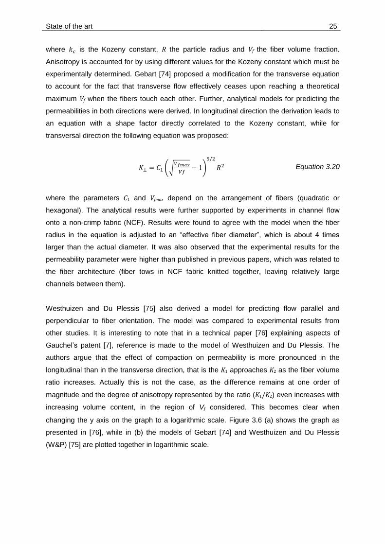
where 𝑘𝑐 is the Kozeny constant, R the particle radius and Vf the fiber volume fraction.
Anisotropy is accounted for by using different values for the Kozeny constant which must be
experimentally determined. Gebart [74] proposed a modification for the transverse equation
to account for the fact that transverse flow effectively ceases upon reaching a theoretical
maximum Vf when the fibers touch each other. Further, analytical models for predicting the
permeabilities in both directions were derived. In longitudinal direction the derivation leads to
an equation with a shape factor directly correlated to the Kozeny constant, while for
transversal direction the following equation was proposed:
𝐾⊥ = 𝐶1 (√
𝑉𝑓𝑚𝑎𝑥
𝑉𝑓− 1)
5/2
𝑅2 Equation 3.20
where the parameters C1 and Vfmax depend on the arrangement of fibers (quadratic or
hexagonal). The analytical results were further supported by experiments in channel flow
onto a non-crimp fabric (NCF). Results were found to agree with the model when the fiber
radius in the equation is adjusted to an “effective fiber diameter”, which is about 4 times
larger than the actual diameter. It was also observed that the experimental results for the
permeability parameter were higher than published in previous papers, which was related to
the fiber architecture (fiber tows in NCF fabric knitted together, leaving relatively large
channels between them).
Westhuizen and Du Plessis [75] also derived a model for predicting flow parallel and
perpendicular to fiber orientation. The model was compared to experimental results from
other studies. It is interesting to note that in a technical paper [76] explaining aspects of
Gauchel’s patent [7], reference is made to the model of Westhuizen and Du Plessis. The
authors argue that the effect of compaction on permeability is more pronounced in the
longitudinal than in the transverse direction, that is the K1 approaches K2 as the fiber volume
ratio increases. Actually this is not the case, as the difference remains at one order of
magnitude and the degree of anisotropy represented by the ratio (K1/K2) even increases with
increasing volume content, in the region of Vf considered. This becomes clear when
changing the y axis on the graph to a logarithmic scale. Figure 3.6 (a) shows the graph as
presented in [76], while in (b) the models of Gebart [74] and Westhuizen and Du Plessis
(W&P) [75] are plotted together in logarithmic scale.

26 State of the art
(a) (b)
Figure 3.6: Curves of permeability of a unidirectional fiber stack in longitudinal and
transverse direction: (a) as presented in [76]; (b) Comparison of W&P and
Gebart models
A comparison between the curves reveals that the models diverge from each other in the
range of fiber volume contents of rovings in pultrusion, which is typically between 0.5 and
0.7. Both models predict a difference of about one order of magnitude between K1 and K2 for
this range of Vf.
Blaurock [29] measured the permeability in the longitudinal direction only for different fiber
volume fractions. The testing assembly allows the fibers to be stretched on the edges. A
Kozeny-Carman constant was fitted to the results. Ding et al. [10] used a similar approach as
Blaurock, but the rovings were cut to a defined length and placed into a channel flow type
testing assembly, i.e. they are not stretched. Measurements were also only performed in the
longitudinal direction. Values for the transversal permeability were estimated from the model
of Westhuizen and Du Plessis [75].
Bates et al. [77] measured only the transverse permeability with an out-of-plane experimental
assembly. No detailed information is given about how the rovings are placed and/or
stretched inside the mold. Scattering of the void fractions for a certain applied compressive
stress suggests that this assembly might be highly sensitive to the laying of fibers in the
mold.
0.0 0.1 0.2 0.3 0.4 0.5 0.6 0.7 0.8 0.9
10-7
10-6
10-5
10-4
10-3
10-2
10-1
100
101
102
103
104
K/r
2
Vf
K1/r2 (W&P)
K2/r2 (W&P)
K1/r2 (Gebart quad)
K1/r2 (Gebart hex)
K2/r2 (Gebart quad)
K2/r2 (Gebart hex)
0
10
20
30
40
50
60
70
80
90
100
K1/K
2 (W&P)
K2
/K1
State of the art 27
Schell et al [78] determined experimentally the permeabilities in both longitudinal and
transverse orientations for glass fiber bundles stretched by winding them around a frame
which is then placed inside the permeability measurement cell. The cell measures by a linear
technique, i.e. separate measures for longitudinal and transverse permeabilities are needed.
Measurements are reported for fiber volume contents of 40% and 64%. (K1/K2) amounted to
4.9 and 2.2 for these fiber volume contents respectively.
3.4 Modelling and simulation
As any physical process, the composite processing can be modelled by the fundamental
laws of conservation of mass, momentum and heat transfer. Specifically, in pultrusion, these
fundamental governing equations, generally with simplifications according to the aspects
being studied, are the basis for the numerical solution. Depending on the derivation
approach, one can obtain the equations in integral (control volume approach) or differential
(infinitesimal volume approach) form. Regarding the framework of analysis, one can derive
the equations for a stationary volume element in space, leading to equations in the so called
Eulerian framework or for a volume element travelling in space, obtaining equations in the
Lagrangian framework. The equations that result from both frameworks are completely
equivalent and can be also derived from one another. Anderson [79] pointed out that in some
cases, in flows with very high speeds (especially when discontinuities are involved, for
example in shock waves), a numerical scheme based on the integral form might be
preferable due to results with better precision. In the following discussion, the differential
form of the equations will be presented, as these are applied for the finite volume solution
method implemented by the CFD code employed.
The continuity equation describes the conservation of mass in a system:
𝜕𝜌
𝜕𝑡+ 𝛻 ∙ (𝜌v) = 0 Equation 3.21
The momentum equation states that the rate of change of momentum in a fluid particle
equals the sum of forces acting upon it. It is written in its most general form as:
𝜕(𝜌v)
𝜕𝑡+ 𝛻 ∙ (𝜌 v⨂v) = −𝛻𝑃 + 𝛻 ∙ 𝝉 + 𝑆𝑀 Equation 3.22

28 State of the art
Where 𝜌 is the density, v is the velocity vector, 𝝉 is the stress tensor and 𝑆𝑀 is a source term
of body forces acting from a distance, e.g. gravitational forces. Taking a Cartesian coordinate
system, Equation 3.22 reduces, for example, for the x component:
𝜕(𝜌𝑣𝑥)
𝜕𝑡+ 𝛻 ∙ (𝜌𝑣𝑥v) = −
𝜕𝑃
𝜕𝑥+
𝜕𝜏𝑥𝑥
𝜕𝑥+
𝜕𝜏𝑦𝑥
𝜕𝑦+
𝜕𝜏𝑧𝑥
𝜕𝑧+ 𝜌𝑓𝑥 Equation 3.23
The governing flow regime in pultrusion can be considered as a Stokes or creeping flow, due
to the relatively high viscosities involved and the short length scale of flow given by the
porous medium.
The energy conservation equation is given by:
𝜕(𝜌𝐻)
𝜕𝑡= −𝛻 ∙ (𝜌 v 𝐻) + 𝛻 ∙ (𝜆 𝛻𝑇) + 𝜏: 𝛻v + 𝑆𝐸 Equation 3.24
where the energy is considered in terms of enthalpy 𝐻. 𝜆 is the thermal conductivity. This so
called thermal energy equation is obtained from the more general total energy equation by
neglecting the kinetic energy term (which is a reasonable assumption for low speed flows)
and variable density effects (appropriate for liquids) [66]. For steady state flow regimes of low
speed, i.e. with negligible viscous dissipation, Patankar [80] proposed further simplification of
Equation 3.24 to:
𝛻 ∙ (𝜌 v 𝐻) = 𝛻 ∙ (𝜆 𝛻𝑇) + 𝑆𝐸 Equation 3.25
Energy source
Rate of energy change by viscous dissipation (irreversible)
Rate of energy change by heat conduction
Net rate of energy change by convective transport
Rate of energy change by unit volume
Body force acting on fluid element
Contribution of shear stresses to the net surface force
Contribution of pressure acting on fluid element to the net surface force
Rate of momentum change of a fluid element
Contribution of normal stress to the net surface force

State of the art 29
The energy source corresponds to the rate of heat generated by the exothermic reaction,
and can be expressed as:
𝑆𝐸 = (1 − 𝑉𝑓)𝜌 𝐻𝑅
𝑑𝛼
𝑑𝑡 Equation 3.26
The method proposed by Patankar for discretization and numerical solution has been widely
used for solving pultrusion-related models. His method and other solving techniques will be
briefly presented in the next section.
3.4.1 Numerical solving techniques
In a numerical procedure, one is concerned with finding the values of unknown variables at
specific locations (grid points or nodes) within a calculation domain (which may be assumed,
for example, as a two-dimensional area space or three-dimensional volume). For calculating
the unknown variable in a grid point adjacent to another at which the variable value is known,
one recurs to a simplified form of the related differential equation (e.g. Equation 3.26), called
the discretization equation. In subdividing the domain into sufficiently small elements with
associated grid points, the discretization equations can be chosen as simple algebraic
equations.
Discretization methods have been traditionally divided into finite difference (FDM), finite
element (FEM) and finite volume (FVM). Patankar noted, however, that a strict separation
among methods might not be useful, and that his own developed methods have the
appearance of finite difference formulations but incorporate ideas of the FE method [80]. All
the three methods have been used for solving CFD problems. Much of recent research has
focused on the application of unstructured grids to discretize complex domain geometries.
A particular advantage of commercial CFD software such as Ansys CFX over self-written
code is the possibility of studying more complex geometries, and the higher flexibility in
creating unstructured meshes for these geometries, without the burden of setting up
algorithms able to properly solve the conservation equations over the discretized domain.
ANSYS CFX uses an element-based finite volume method. The discretization and
subsequent calculation is done over control volumes, defined from groups of mesh elements.
The mesh elements are always three-dimensional in FVM; for simplicity however, the
concept of the control volume is shown in Figure 3.7 in two-dimensional form [81].

30 State of the art
Figure 3.7: Representation of control volume formed by adjacent mesh elements [81]
All solution variables are stored at the nodes (mesh vertices). A control volume (the shaded
area) is constructed around each mesh. By the FVM, the conservation equations of mass,
momentum and energy described in the previous section are integrated over each control
volume, generating volume (representing source terms) and surface (representing fluxes)
integrals. These volume and surface integrals are then discretized to algebraic form, which
are then solved for each control volume. The results for each control volume are then
compared and balanced to the adjacent control volumes and/or boundary conditions by
means of an iterative procedure, until a desired residual coefficient (representing an average
of solution mismatches between control volumes) is reached.
3.4.2 Modelling and simulation of the pultrusion die
Since the pioneering work from Price [23], a number of researchers have dealt with the topic
of modelling and simulating the pultrusion process. Different aspects and/or physical
processes have been primarily considered in the studies, which can be assigned to one of
the following categories:
Thermo-chemical modelling
Fluid dynamics modelling
Thermo-mechanical modelling
The modelling and simulation strategy is strongly dependent on the main physical process
being investigated. To define the physical process(es) relevant to the investigation, it is
useful to examine a schematic representation of the pultrusion die and the phase changes
occurring within it, such as presented by Starr [4]:
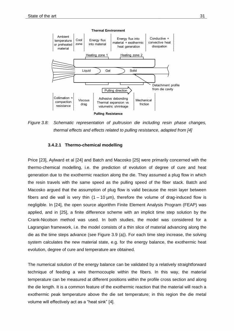
State of the art 31
Figure 3.8: Schematic representation of pultrusion die including resin phase changes,
thermal effects and effects related to pulling resistance, adapted from [4]
3.4.2.1 Thermo-chemical modelling
Price [23], Aylward et al [24] and Batch and Macosko [25] were primarily concerned with the
thermo-chemical modelling, i.e. the prediction of evolution of degree of cure and heat
generation due to the exothermic reaction along the die. They assumed a plug flow in which
the resin travels with the same speed as the pulling speed of the fiber stack. Batch and
Macosko argued that the assumption of plug flow is valid because the resin layer between
fibers and die wall is very thin (1 – 10 µm), therefore the volume of drag-induced flow is
negligible. In [24], the open source algorithm Finite Element Analysis Program (FEAP) was
applied, and in [25], a finite difference scheme with an implicit time step solution by the
Crank-Nicolson method was used. In both studies, the model was considered for a
Lagrangian framework, i.e. the model consists of a thin slice of material advancing along the
die as the time steps advance (see Figure 3.9 (a)). For each time step increase, the solving
system calculates the new material state, e.g. for the energy balance, the exothermic heat
evolution, degree of cure and temperature are obtained.
The numerical solution of the energy balance can be validated by a relatively straightforward
technique of feeding a wire thermocouple within the fibers. In this way, the material
temperature can be measured at different positions within the profile cross section and along
the die length. It is a common feature of the exothermic reaction that the material will reach a
exothermic peak temperature above the die set temperature; in this region the die metal
volume will effectively act as a “heat sink” [4].

32 State of the art
(a) (b)
Figure 3.9: Discretization models of a pultrusion die. (a) Lagrangian framework with moving
slice of material along the die length; (b) Eulerian framework with die cavity
discretized into elements fixed in space
The majority of subsequent studies have applied a Eulerian framework, such as depicted in
Figure 3.9 (b). One reason for this has certainly been the advances in computational
capabilities, allowing even models with several thousands of nodes to run in personal
computers. While both models might deliver similar results in respect of the thermo-chemical
modelling, a transient approach has clear limitations if one is concerned with the fluid
dynamics. Even if there are available methods for the linearization of the continuity and
momentum equations in non-conservation form, a modelling approach such as in Figure 3.9
(a) will fail to catch any long range effect on the flow balances, for example, a boundary
condition is not defined for the outlet in this case. This means that the iteration procedure
becomes more complicated, counterbalancing the simplicity of the computational domain.
Another drawback of the transient method is the limitation of die geometry to a constant
cross section, thus preventing it to be used for studying geometric features such as a
tapering of the die inlet or an injection chamber.
3.4.2.2 Fluid dynamics modelling
In fluid dynamics modelling, one is concerned with pressure and velocity fields of the liquid
resin, i.e. the inlet and the straight cross section located immediately after the inlet. As a
general rule, the die cavity is represented by a homogeneous porous domain through which
the liquid resin permeates by pressure driven flow and at the same time is pulled along with
the reinforcement (advection term). Considering a simplified 2D case of a profile being pulled
through a pultrusion die like the one depicted in Figure 3.9 at constant pulling speed U, i.e. at
steady state, the continuity equation (Equation 3.21) reduces to:

State of the art 33
𝜕(∅𝑣𝑥)
𝜕𝑥+
𝜕(∅𝑣𝑦)
𝜕𝑦= 0 Equation 3.27
where ∅ is the porosity of the reinforcement stack. The momentum equations (Equation 3.22)
in the pulling direction (x) and out-of-plane direction (z) simplify to:
𝑣𝑥 = 𝑈 −
𝐾1
𝜂∅
𝜕𝑃
𝜕𝑥 Equation 3.28
𝑣𝑧 = −
𝐾2
𝜂∅
𝜕𝑃
𝜕𝑧 Equation 3.29
The research group at Ole Miss has done extensive work on this topic. The effect of
processing parameters such as pulling speed, porosity and viscosity on the resin pressure
rise was investigated in [82], [83], [84] and [85], while the effect on pressure of different inlet
geometries, such as a radius, parabolic and conical tapering angle at the entrance was
discussed in [85] [84] [86]. An interesting aspect of their experimental method was the
measurement of pressure within the pultruded material; in an analogous method to the wire
thermocouple, a fiber optic pressure probe was fed to the reinforcement fiber stack. Although
the probe has a relatively large diameter (0.8 mm, die cavity thickness 3.18 mm) which might
arguably produce a local disturbance in the flow, the authors presented a good agreement
between predicted and measured pressure data. More recently, the research group has
published studies dealing with closed injection pultrusion, which will be discussed in detail in
section 3.4.3.
The pressure is usually the most important variable for practical purposes. It is generally
accepted that the pressure increase arising from compaction of the fiber stack soaked with
resin is the main drive for void reduction; the entrapped air can exit at the die inlet through
backflow more easily than the resin, and this is a pressure-driven Darcy’s flow. Another
important aspect is the contribution of fluid resin pressure on the pulling force, which is
arguably the most important experimental variable for process monitoring. Models proposed
for the pulling force are discussed in section 3.4.2.4.
Some researchers have proposed analytical models for the pressure inside the pultrusion
die. Kim et al [27] proposed an analytical model for pressure by assuming unidirectional flow
in the pulling direction, justified by the permeability in transverse direction being much lower
than in the longitudinal one. They derived a solution for the pressure gradient along the inlet
portion:

34 State of the art
𝑑𝑃
𝑑𝑥=
𝑈𝜂
𝐾(𝑥)[1 − 𝑉𝑓𝑥 − (1 −
∆𝜈
𝜈) (
𝑉𝑓𝑥
𝑉𝑓− 𝑉𝑓(𝑥)) ] Equation 3.30
where 𝑈 is the pulling speed, 𝐾(𝑥) is the longitudinal permeability, and 𝑉𝑓𝑥 is the fiber volume
fraction as functions of axial distance. ∆𝜈/𝜈 represents the resin volume change, given by the
sum of thermal expansion and shrinkage due to curing effects:
∆𝜈 𝜈⁄ = 𝛼𝜈∆𝑇 − 𝛽∆𝛼 Equation 3.31
where 𝛼𝜈 is the thermal expansion coefficient and 𝛽 is the coefficient of volumetric shrinkage
of resin due to curing. A viscosity model such as given by Equation 3.15 was also applied.
Integration of Equation 3.30 gives a pressure distribution along the tapered inlet. By
neglecting volume change effects in the inlet section and integrating, the following pressure
distribution is obtained:
𝑃(𝑥) =
𝑈𝜂
𝐾(𝑥)[1 −
𝑉𝑓𝑥
𝑉𝑓 ] 𝑥 Equation 3.32
Blaurock [29] derived a similar analytical model for the pressure build up in the inlet region.
He also argued that besides liquid pressure build-up due to compaction and resin backflow,
another contribution to pressure arise from a supporting effect of the fibers. He used
Gutowski’s model for the transversal stiffness of a fiber stack (Equation 3.17) to estimate this
contribution. Ding et al [10] also proposed an analytical model for pressure rise in a tapered
closed injection die (see section 3.4.3).
3.4.2.3 Thermo-mechanical modelling
Thermo-mechanical modelling has not been widely studied for the specific case of pultrusion,
although issues of internal stresses and warping are known and generally assumed to be
intrinsic to pultruded products. Recently however, extensive work by Baran has dealt with
this topic. In his studies, the stresses developed due to processing, mainly due to thermal
expansion and shrinkage, are evaluated and translated into internal stresses in the final
product and/or warpage. He listed the main mechanisms which act during processing and
generate internal stresses and distortions as:

State of the art 35
Different coefficients of thermal expansion (CTE) of the thermosetting resin and the
reinforcements
Different CTE between layers of different reinforcement materials and anisotropy within
layer, that is, different CTE in the in-plane and out-of-plane directions
Resin shrinkage during curing reaction
Temperature and cure gradients inside the composite material, especially for thick parts
Interaction between the heated die and the part
In [87], Baran presented a model for analyzing process induced stresses and distortions by
sequential coupling of a 3D stationary thermo-chemical model (Eulerian framework) with a
2D transient mechanical model (Lagrangian framework) using two different solving methods:
the control volume based finite difference (CV/FD) and the finite element with nodal control
volume (FE/NCV).
The CV-FD model was implemented in MATLAB and was based on the model firstly
proposed by Bogetti and Gillespie [88], [89]. In [88], they described a solving procedure for
the temperature and degree of cure in a 2D field, in which fibers are aligned in one of the
solving coordinate directions, the other being the through-thickness direction. By means of a
coordinate system transformation technique, more complex geometries can be calculated,
such as L-shapes and varying thicknesses. In [89], they presented an in-plane stress-strain
calculation procedure based in a simplified solving method for temperature and degree of
cure in the through-thickness direction only.
Johnston et al [90] presented a more generalized version of this method, in which the fiber
orientation in each ply may vary relatively to the plane chosen for the calculation. In Figure
3.10 for example the ply 𝑖 is oriented at an angle 𝜃𝑖 relatively to the plane 𝑥′ ̵ 𝑧′ assumed for
the model. A transformation from the 𝑥′ ̵ 𝑧′ to the 𝑥 ̵ 𝑧 plane is made through the angle 𝛽 for
complex shape geometries. The method applies a plane strain assumption for the calculation
of stresses and distortions in the out-of-plane orientation to predict effects such as spring-in.
In the model presented by Baran, the plane is a cross section of the pultruded profile, i.e. the
fibers are oriented in the out-of-plane direction relative to the plane chosen for the stress-
strain calculation. In [91], Baran expanded the mechanical model to a volume of 3D elements
traveling through the die, thus being able to also account for stresses in both longitudinal and
transverse directions. In [92] and [93] he modelled L-shape and rectangular profiles
composed of rovings and CFM layers. In [94], he analyzed the impact of process induced
stresses by transferring the results to a subsequent structural mechanics simulation.

36 State of the art
Figure 3.10: Composite part assumed for plane stress-strain model by Johnston et al [90].
(a) isometric view showing ply orientation; (b) plane view showing principal
plane directions and reference plane
3.4.2.4 Modelling of pulling force
Analysis of the force needed to pull the pultruded profile through and out of the die and the
contributions to this pulling force arising from different sections of the process is arguably the
most important aspect to understanding the pultrusion process. Some authors have also
addressed this topic, reaching in some cases very differing results. In general, a combination
of analytic and numerical solutions has been applied to sum up the different contributions to
the pulling force.
Kim et al [27] described the pulling force as arising from two different sources. The first one
occurs in the tapered inlet region from pressure build-up associated with compaction of the
wetted out reinforcement material. The resistance in this region is the axial component of the
force due to pressure against the mold wall. The other source arises in the constant cross
section of the die, by the friction between the resin in liquid and gel phase, up to the point
where the resin detaches from the die wall due to shrinkage.
The force per unit length in the opposite pulling direction in the tapered section due to
compaction of the wetted out reinforcement 𝜎𝑐 is calculated from the pressure function
(Equation 3.32) by:
𝜎𝑐 = 𝑃(𝑥) 𝑠𝑖𝑛 𝜃 Equation 3.33
State of the art 37
Where 𝜃 is the tapering angle. Integration of Equation 3.33 over the tapered length gives the
contribution of compaction of the reinforcement material to the pulling force. Kim argued that
further pressure increase can occur in the straight portion of the die due to thermal
expansion; therefore Equation 3.30 was also applied to the straight section. Another
assumption was that a thin layer of resin exists between the bulk composite and the die inner
wall; within this thin resin layer in the immediate vicinity to the wall gels faster, generating
thus Coulomb friction directly proportional to the pressure, exerted over the wall. The
pressure however, is smaller than predicted by Equation 3.30 due to a shielding effect
caused by the same gelled layer. A fully implicit transient finite element method was used for
the numerical calculations (see Figure 3.9 (a)). They compared predictions from numerical
calculations with measured values of pulling force, finding good agreement to support the
model.
Blackrock [29] presented a similar approach by calculating the contribution of a pressure
function (see section 3.4.2.2) to the total pulling force. He also used the same assumption of
a thin resin film between die wall and composite bulk, estimating its thickness at about 3 µm.
He calculated for a given system the cumulated contributions to pulling force approximately
as follows:
15% due to compaction of wetted out reinforcement material arising in the inlet (radius
entrance)
5% due to shearing of the viscous resin layer arising in the liquid region up to the gel
point
80% due to friction in the straight section of the die (compaction of reinforcement and
pressure from thermal expansion), up to the point where the shrinkage effect due to
curing excels the thermal expansion, i.e. the profile detaches from the die inner walls
Li et al [12] [33] did an experimental study on pulling force, applying different techniques. For
example, they used a “mat tracer” method, i.e. feeding a small piece of CFM to produce local
higher fiber volume content while it travels through the die. By doing comparing experiments
with dies of different lengths, they supported the thesis of the negligible contribution of the
downstream part of the die to the pulling force. They also found the pulling resistance in the
liquid region to be independent of pulling speed. Finally, they used an especially designed
testing assembly to characterize the friction coefficient of the resin in the gel and post-gel
regions, deriving an analytical model as a function of temperature and conversion. They
concluded that the larger resistance to pulling comes from the gel and post-gel zone up to
the detachment point, due to a simultaneous increase in thermal expansion stress and

38 State of the art
friction coefficient. They argued that the direct correlation between pulling speed and force is
actually explained by an increase of the gel zone length with increasing speed. This is a
direct contradiction of the resin film model proposed by Blaurock and Kim et al.
Carlone et al [95], on the other hand, concluded that the viscous drag in the liquid resin
region was the main contribution to pulling resistance of a rod profile, while the compaction of
material at the die inlet was found to have a negligible effect.
3.4.3 Simulation of the closed injection process
A number of research groups have already proposed models for the pultrusion process with
some sort of closed injection and impregnation technique. The focus of these studies is
usually on flow simulation especially in the injection zone in order to predict flow and
pressure fields.
Kommu et al [35] and Voorakaranam et al [96] studied flow patterns for a die with a hole for
injecting resin in the straight section, that is, without an injection cavity. Mustafa et al [36]
used the same approach, but compared the results with tapered inlets of different taper
angles.
Ding et al [10] evaluated a tapered die with a design according to Gauchel [7]. He solved the
continuity equation with Darcy’s law numerically using the CV/FEM technique to obtain a
pressure field in the inlet section. Additionally, he proposed an analytical solution for the
pressure by simplifying the model to one-dimensional flow, and deriving a pressure
contribution from drag flow and a pressure flow induced by the resin injection. The numerical
and analytical solutions were very close to each other and showed good agreement with
experimental results as well.
Liu [97] [98] used a NV/FEM technique to model flow within a pultrusion die. The die was
modelled with a constant cross section, and resin was injected through a single hole at a
distance of 100 mm from the inlet. He also derived an analytical solution for one-dimensional
flow over the entire die length; however, he did not consider any thermal expansion or
shrinkage effects, such that the pressure follows a linear decay from the injection point to
both inlet and outlet of the die.
Srinivasagupta et al [13] models included predictions of pressure at the die inlet, temperature
along the die and pulling force for a specific die design with resin injection.

State of the art 39
The research group at Ole Miss presented a number of numerical studies of a die with
conical inlet geometry. Rahatekar [99] studied the effects of several parameters (pull speed,
fiber volume fraction, resin viscosity and taper angle) on the fiber wet out. He employed a
finite volume method as proposed by Patankar and introduced a fill factor to predict whether
a particular region is properly wetted out with resin. In [100] he expanded his model to a
multilayer reinforcement composed of mats and rovings. Jeswani [101] used the same
model to study a design with multiple injection ports and different locations along the length
of the tapered section. His goal was to obtain a prediction of wet-out for varying composite
thicknesses and high pulling speeds (about 1.5 and 3.0 m/min). Ranga [102] investigated the
effect of chamber length, taper angle and pulling speed on wet-out. Palikhel [103] compared
a conical inlet attached to the die with the same inlet detached, i.e. with a gap between inlet
and die. All of these studies lack comparison with real processing experiments.
Connolly et al [11] focused on flow simulations in the conical inlet region of the die using the
commercial software Ansys CFX. The pressure at the resin injection nozzle predicted by the
simulation was in agreement with measured values, the measured pressure near the
transition from taper to straight die section was however much higher than predicted by the
simulation, which was attributed to factors such as roving twist or resin/fiber interactions
which were not represented in the model.
40 Resin characterization and modelling
4 Resin characterization and modelling
In this section, the experimental work done on the chemorheological characterization of the
studied resin system is described, i.e. the evolution of reaction rate as a function of time and
temperature as well as the changes in resin physical state as curing progresses. Firstly, the
resin formulation is presented along with applied experimental methods, namely DSC and
rheology measurements. In the following Subsections, results obtained from each of the
methods are then presented along with the development of models for the prediction of the
resin properties throughout the curing process.
4.1 Materials and methods
A description of the resin formulation subjected to the characterization work is given in this
section, including the several additives and their respective functions in the curing and/or
pultrusion processing. Subsequently, the procedure applied for the measurements and the
corresponding sample preparation are described.
4.1.1 Resin system
The resin system used in this work is a formulation based on a two-step-curing resin named
Daron ZW 015864 (Aliancys, Zwolle, NL) (see section 3.1.3). The resin consists of a
prepolymer diluted in styrene (solids content 63.5% – 66.5%) and premixed with an inhibitor.
The inhibitor hinders unwanted polymerization during storage, thus prolonging shelf life.
The resin can be processed to a composite part through the combination of pultrusion and a
post-forming step. Pultrusion is therefore, in this case, the means for producing a B-staged
preform. The first reaction step (B-staging) progresses relatively slowly at room temperature,
or may be accelerated by the addition of a catalyst. The second reaction step (radical
polymerization) is initiated by the peroxide splitting into free radicals at a higher temperature
level. Alternatively, the resin can be fully cured within the pultrusion die by setting the die to a
higher temperature level, e.g. 150 °C. In order to undergo curing through the two-step
processing route, the resin must be formulated by mixing of different components and
additives, which are listed below:
Di-isocyanate (MDI): the isocyanate groups react with hydroxyl functional groups present
in the prepolymers backbones by polyaddition in the B-staging. This reaction results in
the formation of a weakly cross-linked network, similar in consistency to rubber

Resin characterization and modelling 41
Catalyst: the catalyst accelerates the B-staging reaction to take place within the
pultrusion die. Catalyst amount is adjusted so that B-staging is reached between 2 and
10 min at a temperature range of 80 °C – 100 °C
Internal mold release (IMR): this is an essential processing additive for reducing
adherence of the resin to the die inner walls during curing
Organic peroxide: initiates the second reaction step by splitting into free radicals at a
certain temperature level. The triggering temperature, typically between 100 °C – 120 °C
can be defined by selection of an appropriate peroxide
In the initial screening it was found that the resin reactivity is extremely sensitive to the
amounts of other components added, specially the ratio of catalyst and IMR. The IMR
effectively slows down the reaction, so that by adding IMR, one has to increase the catalyst
amount in order to obtain the same reactivity. The resin formulation shown in Table 4.1 was
applied in all characterization investigations.
By separately premixing the A and B components, no reaction takes place. This is important
since the first reaction step starts directly upon mixing of A and B, as usual with fast reacting
polyurethane systems.
Table 4.1: Resin formulation applied throughout this work
Resin component Parts per weight
(ppw)
A Component
Daron ZW 015864 100
Catalyst 1.0
IMR 2.0
B Component
MDI 25
Peroxide 1.0
The resin system was characterized with focus on obtaining models for the cure kinetics, flow
behavior and shrinkage evolution throughout curing. These models are used as input in the
simulation studies. In the following sections, the characterization methods and the models
obtained will be described in detail.

42 Resin characterization and modelling
4.1.2 Differential Scanning Calorimetry (DSC)
DSC was applied as a method to detect the development of cure from liquid resin to fully
cured thermoset matrix. Calorimetric measurements were performed with a Netzsch DSC204
F1 Phoenix. Dynamic scan measurements were carried out at different linear temperature
ramps (0.5 K/min, 1.0 K/min, 5.0 K/min) from -20 °C to 185 °C. This was followed by cooling
down to room temperature at 5 K/min and a second heating step to assess whether residual
reaction takes place. It is inevitable that a small portion of the reaction is not captured by the
characterization method. In order to keep this error as low as possible, efforts are made to
obtain a precise mixing ratio while at the same time starting the measurement as soon as
possible. For the sample preparation, the following procedure was applied:
1. Cooling down of the DSC furnace to +5 °C
2. Weighting of the A and B components in a precision balance (accuracy 0.001 g)
3. Mixing by hand for 30 s
4. Metering of 16 - 18 mg to the DSC pan by a high precision pipette (accuracy 1 µL)
5. Sealing the DSC pan and placing it into the DSC sample holder
6. Cool down to -40 °C at maximum cooling rate (approximately 50 K/min)
Steps 2 through 5 were conducted in all measurements in approximately 2 min. Three
replicates were measured for each heating rate. Results show reproducible curves for all
measured scans. Typical DSC curves obtained for the three heating rates measured are
shown in Figure 4.1. Characteristic values obtained from the plot analysis are listed in Table
4.2. The onset is typically defined as the point of intersection of two tangents, one at the
inflection point during the reaction and the other at the linear baseline, denoting start and end
of the reaction, respectively. The peak is determined at the highest value within the reaction
stage. The area is calculated between the DSC plot and the baseline defined by the tangent
traced between a point in the flat region before the onset of reaction and another after the
end of reaction.
4.1.3 Rheology measurements
Rheology measurements in oscillation mode were carried out to evaluate flow behavior as
the resin goes from liquid to cured state. A MCR301 rheometer (Anton Paar GmbH) in the
disc-plate configuration according to DIN 53018-1 was used for the measurements. The top
disc has a diameter of 25 mm. The measurements were carried out under 1 Hz frequency
(corresponding to an angular frequency of 6.28 rad/s) and amplitude of 0.16 mrad of

Resin characterization and modelling 43
deflection angle (corresponding to a strain amplitude of 0.2 %). A controlled normal force of
zero N is kept constant throughout the measurement, while the gap is adjusted. Dynamic
scan rates of 1.0 K/min and 5.0 K/min were applied from 5 °C to 180 °C. The following
procedure was followed in the preparation of samples for rheology measurements:
1. Cooling down of the rheometer chamber to +5 °C. Since the maximum cooling rate is
much lower than in the DSC, the initial temperature is set as low as possible to hinder
early stage reaction, but also preventing accumulation of condensed water from ambient
air
2. Weighting of the A and B components in a precision balance (accuracy 0.01 g)
3. Mixing by hand for 30 s
4. Pouring of approximately 1 g to the center of the rheometer bottom plate
5. Lowering the upper disc close to the gap set for the measurements (1 mm)
6. Removal of resin excess at the disc edges
7. Start of measurement
Steps 2 through 7 were done in all measurements within 3 - 4 min. Due to the slower
preparation procedure and the larger resin amount needed for the measurement, it is
expected that a larger amount of the curing reaction has taken place at the time the
measurement is started, as compared to DSC.
The values of storage (𝐺′) and loss (𝐺′′) moduli in shear are obtained from the
measurements (equations 3.6 to 3.10). From these values, the apparent viscosity of the
sample is calculated according to equations 3.11 to 3.14. In the following discussion,
wherever the term viscosity is used, it actually refers to the modulus of the complex viscosity
(see Section 3.2.2).
4.2 DSC measurement results
Typical measurements of heat flow plotted against the temperature are given for the applied
heating rates in Figure 4.1. The two reaction steps can be clearly separated for all heating
rates measured. The first flat peak represents the B-staging reaction, while the second sharp
peak is typical of a self-accelerated polymerization, initiated by the splitting of the peroxide
initiator into free radicals. In Figure 4.2, an example of the conducted plot analysis is shown
with the characteristic values obtained from the measurement. The values obtained from
measurements under the different dynamic scans are then listed in Table 4.2.

44 Resin characterization and modelling
Figure 4.1: Heat flow data from DSC measurements at three different heating rates
Figure 4.2: Analysis of DSC data from measurement at a dynamic scan rate of 5 K/min
The onset of the first reaction step occurs very early at approximately 0 °C. No clear
dependence on the heating rate can be attested to the onset, in contrast to all other
characteristic values. This is an indication of process variability arising from the sample
preparation procedure described above. The almost immediate onset is in agreement with
the observation of material behavior upon mixing by hand, in which the material starts to
-20 0 20 40 60 80 100 120 140 160 180 200 220-2.5
-2.0
-1.5
-1.0
-0.5
0.0
heat flow
[m
W/m
g]
Temperature [°C]
5 K/min
1 K/min
0.5 K/min
Exo
-20 0 20 40 60 80 100 120 140 160 180 200 220
-2.5
-2.0
-1.5
-1.0
-0.5
0.0
2nd
reaction step
(Radical polymerization)
Onset 129,0 °C
Onset 1,9 °C
Heat flow
[m
W/m
g]
Temperature [°C]
Area 85 J/g Area 181 J/g
End 88,1 °C
Peak 50,2 °C
Peak 133,2 °C
End 138,2 °C
1st reaction step
(B-staging)

Resin characterization and modelling 45
develop heat shortly after mixing. Due to the preparation procedure, it is inevitable that a
small portion of the first reaction is not caught by the DSC measurements. Since the
measurements were found to be reproducible, the amount of reaction occurring prior to the
measurement is assumed to be negligible. The first reaction step corresponds to
approximately 30% of the total heat of reaction.
Table 4.2: Characteristic values of temperature and heat release for the two-step curing
reaction under different heating rates
1st reaction step
(B-staging) 2nd reaction step
(Radical polymerization) Total Area [J/g] Heating
rate Onset [°C]
Peak [°C]
End [°C]
Area [J/g]
Onset [°C]
Peak [°C]
End [°C]
Area [J/g]
5,0 K/min 1.9 50.2 88.1 85 129.0 133.2 138.2 181 266
1,0 K/min 6.0 22.9 56.5 89 113.0 115.9 119.8 184 273
0,5 K/min -2.9 18.7 46.9 81 103.9 108.1 111.0 165 246
4.3 Kinetic modelling
Fitting of data from DSC measurements was done with the software NETZSCH
Thermokinetics 3.1. The software contains regression methods according to ASTM E698,
Friedman and Ozawa-Flynn-Wall (see section 3.2.1). It is noted that the model developed in
this study is purely empirical, i.e. it does not convey any of the reaction mechanisms which
were qualitatively described in Section 3.1.3. The regression procedure within the software is
well explained in [21]. An initial model composed of reaction steps is chosen for modelling a
multi-step reaction mechanism. The type of model is chosen based on appearance of the
DSC heat flow curves. A nonlinear least-squares fitting method is then applied for data
regression and fitting of optimum parameters. Calculation of regression values is done by
means of a Runge-Kutta method of 5th grade. Minimization of the sum of least square values
is done by the Gauss-Newton method.
In the present case, fitting of data was attempted by setting two different models. A first
approximation was done applying two reaction steps in series, in analogy to the two reaction
mechanisms of B-staging and final curing discernible in DSC. The model is similar to the final
three-step model described in Equations 4.1 through 4.4, considering only reaction steps 1
and 2. The fitting procedure executed by applying the two different reaction models leads to
the results shown in Figure 4.3.

46 Resin characterization and modelling
Figure 4.3: Original DSC data and data obtained from fitting to the two-step and three-step
models
It can be seen that a generally good representation of measured data is achieved by the two-
step model. However, the fit for both reactions present a discernible discrepancy from
measured data, as seen by the differences in the peaks and at the end of the second
reaction exotherm. Statistical values for the sum of least square residuals of 9.24 and
correlation coefficient of 0.9887 were obtained. The addition of a third reaction step in the
model leads to a better fitting of the reaction as measured by DSC. A sum of the least
squares residuals of 2.94 and a correlation coefficient of 0.9964 were obtained for the three-
step model. It can be concluded that a better representation of DSC data is achieved by the
three-step in comparison to the two-step model. The final model applied throughout this
study is therefore composed of three sequential reaction steps:
𝐴1→ 𝐵
2→ 𝐶
3→ 𝐷 Equation 4.1
It should be noted that the model is purely empirical, i.e. the three reaction steps in the model
do not imply three different reaction mechanisms taking place during cure. In fact, while
step 1 describes the B-staging reaction, the radical polymerization is described by the
simultaneously occurring steps 2 and 3. For each reaction step, a cure rate dependency
function is fitted in terms of the respective reaction product in the following form:
𝑑𝛼𝑖
𝑑𝑡= 𝐴𝑖 𝑒𝑥𝑝 (
−𝐸𝐴𝑖
𝑅 𝑇) ∙ 𝑓(𝛼𝑖) Equation 4.2
-20 0 20 40 60 80 100 120 140 160 180 200 220-2.5
-2.0
-1.5
-1.0
-0.5
0.0
heat flow
[m
W/m
g]
Temperature [°C]
DSC measured data
5 K/min
1 K/min
0.5 K/min
Two-step model
5 K/min
1 K/min
0.5 K/min
Three-step model
5 K/min
1 K/min
0.5 K/min
Exo
0 20 40 60 80 100
-0.15
-0.10
-0.05
0.00

Resin characterization and modelling 47
where 𝛼𝑖 is the amount of reactant which has converted into a product through reaction step
𝑖 by time 𝑡, i.e. the degree of cure for that particular reaction step, which goes from 0 to 1. 𝐴𝑖
is a pre-exponential factor and 𝐸𝐴𝑖 the activation energy for the reaction step 𝑖. The following
functions were found to fit well the respective reaction steps:
Reactions 1 and 2, nth order
reaction with autocatalysis 𝑓(𝛼𝑖) = (1 − 𝛼𝑖)𝑛𝑖(1 + 𝐾𝑐𝑎𝑡𝑖 𝛼𝑖), 𝑖 = 1, 2 Equation 4.3
Reaction 3, nth order reaction 𝑓(𝛼𝑖) = (1 − 𝛼𝑖)𝑛𝑖 , 𝑖 = 3 Equation 4.4
where 𝑛𝑖 is the reaction order and 𝐾𝑐𝑎𝑡𝑖 an autocatalytic factor for the reaction step 𝑖. Since
the reaction is modelled as a sequence of reaction steps, the rate of reaction for a particular
step depends on the conversion which has already been reached in the previous reaction
step(s). This is done by multiplying the term 𝛼𝑖 by the previous degree of cure 𝛼𝑖−1. The
following reactions are then obtained for each reaction step.
𝑑𝛼1
𝑑𝑡= 𝐴1 𝑒𝑥𝑝 (
−𝐸𝐴1
𝑅 𝑇) ∙ (1 − 𝛼1)𝑛1(1 + 𝐾𝑐𝑎𝑡1 𝛼1) Equation 4.5
𝑑𝛼2
𝑑𝑡= 𝐴2 𝑒𝑥𝑝 (
−𝐸𝐴2
𝑅 𝑇) ∙ (𝛼1(1 − 𝛼2))𝑛2(1 + 𝐾𝑐𝑎𝑡2 𝛼1 𝛼2) Equation 4.6
𝑑𝛼3
𝑑𝑡= 𝐴3 𝑒𝑥𝑝 (
−𝐸𝐴3
𝑅 𝑇) ∙ (𝛼2(1 − 𝛼3))𝑛3 Equation 4.7
The overall degree of cure 𝛼 is given by the weighted sum of the 𝛼𝑖 terms.
𝛼 = 𝐹𝑅1 𝛼1 + 𝐹𝑅2 𝛼2 + 𝐹𝑅3 𝛼3 Equation 4.8
The term 𝐹𝑅𝑖 is the fraction of the reaction step 𝑖 relatively to the total reaction. Since the
DSC analysis is based on the developed exothermic heat of reaction, 𝐹𝑅𝑖 is related to the
contribution of reaction 𝑖 to the overall degree of cure and to the total heat of reaction. The
volumetric internal heat generation term �̇� is given by rearrangement of Equation 3.5.
�̇� = 𝜌 𝐻𝑅
𝑑𝛼
𝑑𝑡= 𝜌 𝐻𝑅 (𝐹𝑅1
𝑑𝛼1
𝑑𝑡+ 𝐹𝑅2
𝑑𝛼2
𝑑𝑡+ 𝐹𝑅3
𝑑𝛼3
𝑑𝑡) Equation 4.9

48 Resin characterization and modelling
The total heat of reaction 𝐻𝑅 in Equation 4.9 is taken as the maximum value obtained in the
DSC measurements (361 J/g). Table 4.3 lists the parameters obtained from fitting of the DSC
data to the three-step model.
Table 4.3: Fitted parameters for final kinetic model according to Equations 4.1 to 4.7
Parameter Reaction step 1 Reaction step 2 Reaction step 3
𝐴𝑖 [s-1] 1.305 x 10⁹ 2.079 x 10⁶ 2.044 x 10³
𝐸𝐴𝑖 [J/mol] 6.971 x 10⁴ 9.798 x 10⁴ 3.1 x 10⁴
𝑛𝑖 2.1709 0.9575 3.9037
𝐾𝑐𝑎𝑡𝑖 0.4956 1.253 x 10⁵ -
𝐹𝑅𝑖 0.2877 0.2496 0.4627
The evolution of the degree of cure can be calculated for a given temperature cycle by
integration of Equation 4.5 to Equation 4.7. The Thermokinetics software can perform such a
calculation for a sequence of constant temperatures and linear heating or cooling rates. A
plot for a series of isotherms is given in Figure 4.4.
Figure 4.4: Degree of cure evolution for a series of isotherms between 70 and 130 °C
The plateau at a conversion of 0.29 (= 𝐹𝑅1) observed in the lower temperature isotherms
depicted above corresponds to completion of the B-staging reaction step. Analysis of this plot
gives insight into the processability of the studied formulation to a B-stage during pultrusion.
0 5 10 15 20 25 30
0.0
0.2
0.4
0.6
0.8
1.0
Degre
e o
f cure
Time [min]
70 °C
80 °C
90 °C
100 °C
110 °C
120 °C
130 °C

Resin characterization and modelling 49
Assuming no substantial temperature increase due to the exothermic heat released in the
first reaction step, one can evaluate for example a die temperature set point of 100 – 110 °C
as safe for pultrusion processing, with a time span of approximately 10 min before the
second reaction is triggered.
4.4 Rheology measurement results
For the modelling of the viscosity evolution throughout the curing, it is necessary to have a
prediction of the degree of cure evolution parallel to the dynamic rheology scan. A
considerable temperature lag between the set temperature of the measuring block and the
real temperature of the sample was observed for the cooling step. Because of that, the
temperature was measured independently by fixing thermocouples to the sample holder on
the upper and bottom plates. A gap of 1.5 mm was kept constant throughout the
measurements. The temperature evolution is shown against the rheometer temperature for a
heating rate of 5 K/min in Figure 4.5. In order to obtain a better estimate of the degree of
cure during a rheology measurement, cure simulations were conducted using the in-house
finite difference algorithm (see Section 7.1.4). One of the simulations applied the temperature
cycle measured in the center of the upper disc as the ambient temperature, the other applied
the temperature at the center of the bottom plate for the curing cycle. The estimate of the
degree of cure was then obtained as the average of the two curves resulting from the
simulations. Results are shown in Figure 4.5.
An uneven temperature distribution can be seen by the difference between the temperatures
at the disc bottom and top. The simulation results indicate that an incipient reaction already
occurs prior to starting a rheology measurement. The absolute value of the degree of cure is
estimated at 0.7% at the beginning of the measurement. Despite this low initial value, the
reaction is already evolving at the beginning of the rheological test, resulting in a much faster
evolution of both reaction steps compared to the predicted by the set temperature signal. The
exothermic peaks of the measured and predicted temperatures at the top disc center are
overlapping, indicating the accuracy of the FD-model. The measured temperature at the
bottom is delayed in comparison to the temperature predicted by the model; this can be
explained by the fact that the thermocouple was located directly above the heating unit
(Peltier element), which forced the temperature to remain close to the rheometer set
temperature. This continued until the bulk of the resin undergoes the radical polymerization.
The heat release in then sensed at the same time by the top and bottom thermocouples.
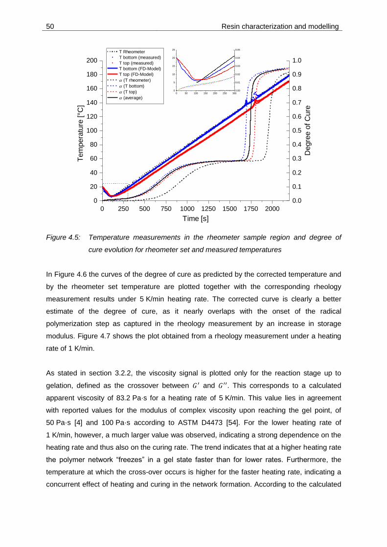
50 Resin characterization and modelling
Figure 4.5: Temperature measurements in the rheometer sample region and degree of
cure evolution for rheometer set and measured temperatures
In Figure 4.6 the curves of the degree of cure as predicted by the corrected temperature and
by the rheometer set temperature are plotted together with the corresponding rheology
measurement results under 5 K/min heating rate. The corrected curve is clearly a better
estimate of the degree of cure, as it nearly overlaps with the onset of the radical
polymerization step as captured in the rheology measurement by an increase in storage
modulus. Figure 4.7 shows the plot obtained from a rheology measurement under a heating
rate of 1 K/min.
As stated in section 3.2.2, the viscosity signal is plotted only for the reaction stage up to
gelation, defined as the crossover between 𝐺′ and 𝐺′′. This corresponds to a calculated
apparent viscosity of 83.2 Pa·s for a heating rate of 5 K/min. This value lies in agreement
with reported values for the modulus of complex viscosity upon reaching the gel point, of
50 Pa·s [4] and 100 Pa·s according to ASTM D4473 [54]. For the lower heating rate of
1 K/min, however, a much larger value was observed, indicating a strong dependence on the
heating rate and thus also on the curing rate. The trend indicates that at a higher heating rate
the polymer network “freezes” in a gel state faster than for lower rates. Furthermore, the
temperature at which the cross-over occurs is higher for the faster heating rate, indicating a
concurrent effect of heating and curing in the network formation. According to the calculated
0 250 500 750 1000 1250 1500 1750 2000
0
20
40
60
80
100
120
140
160
180
200
Tem
pera
ture
[°C
]
Time [s]
T Rheometer
T bottom (measured)
T top (measured)
T bottom (FD-Model)
T top (FD-Model)
(T rheometer)
(T bottom)
(T top)
(average)
0.0
0.1
0.2
0.3
0.4
0.5
0.6
0.7
0.8
0.9
1.0
Degre
e o
f C
ure
0 50 100 150 200 250 3000
5
10
15
20
25
0.00
0.01
0.02
0.03
0.04
0.05
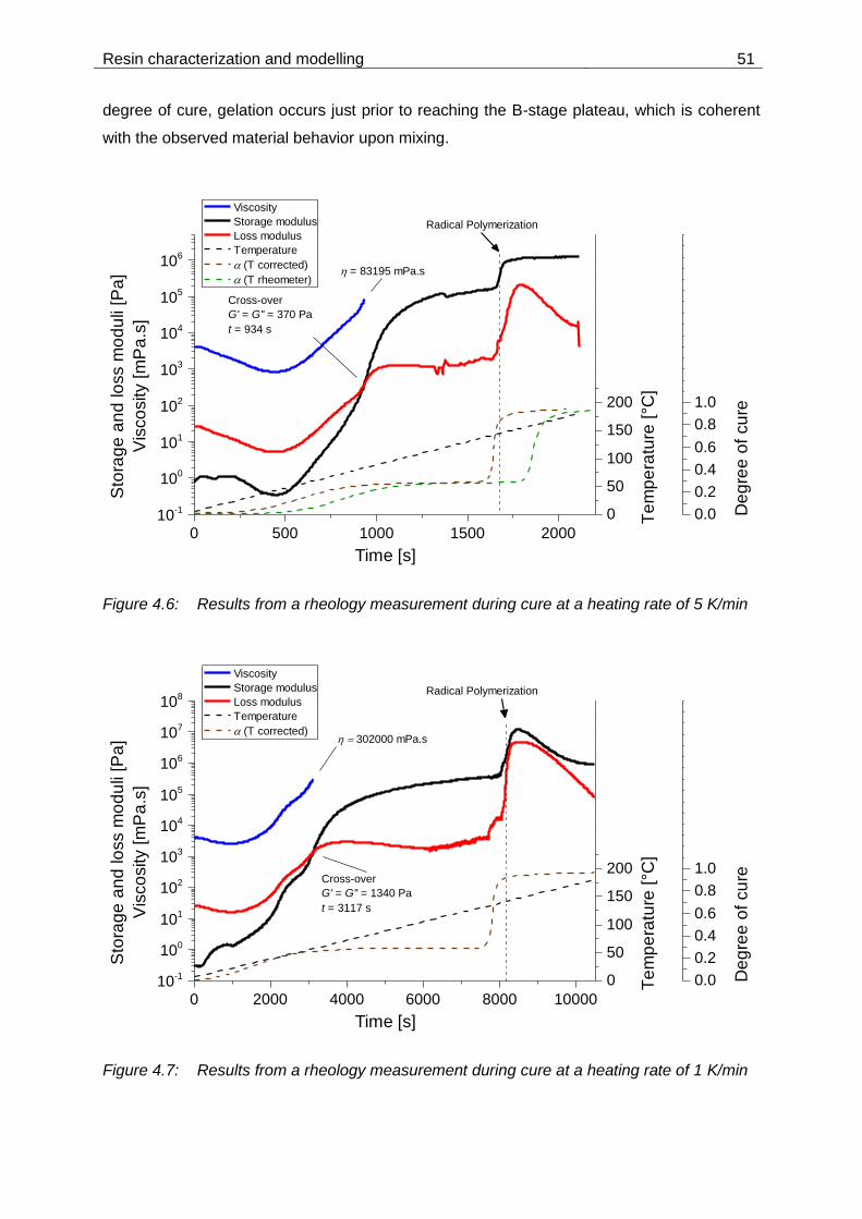
Resin characterization and modelling 51
degree of cure, gelation occurs just prior to reaching the B-stage plateau, which is coherent
with the observed material behavior upon mixing.
Figure 4.6: Results from a rheology measurement during cure at a heating rate of 5 K/min
Figure 4.7: Results from a rheology measurement during cure at a heating rate of 1 K/min
0 500 1000 1500 200010
-1
100
101
102
103
104
105
106
Sto
rag
e a
nd
lo
ss m
od
uli
[Pa
]
Vis
co
sity [
mP
a.s
]
Time [s]
Viscosity
Storage modulus
Loss modulus
Temperature
(T corrected)
(T rheometer)
Cross-over
G' = G'' = 370 Pa
t = 934 s
= 83195 mPa.s
0
50
100
150
200
250
300
350
400
450
500
Te
mp
era
ture
[°C
]
0.0
0.2
0.4
0.6
0.8
1.0
1.2
1.4
1.6
1.8
2.0
2.2
2.4
De
gre
e o
f cu
re
Radical Polymerization
0 2000 4000 6000 8000 1000010
-1
100
101
102
103
104
105
106
107
108
Sto
rag
e a
nd
lo
ss m
od
uli
[Pa
]
Vis
co
sity [
mP
a.s
]
Time [s]
Viscosity
Storage modulus
Loss modulus
Temperature
(T corrected)302000 mPa.s
Cross-over
G' = G'' = 1340 Pa
t = 3117 s
0
50
100
150
200
250
300
350
400
450
500
Te
mp
era
ture
[°C
]
0.0
0.2
0.4
0.6
0.8
1.0
1.2
1.4
1.6
1.8
2.0
2.2
2.4
De
gre
e o
f cu
re
Radical Polymerization

52 Resin characterization and modelling
The observed values for both heating rates are shown in Table 4.4. Three measurements
were considered for each heating rate, and the average values were considered for
evaluation. As already observed during DSC measurements, a better repeatability could be
obtained for the higher heating rate. This is reflected in the higher standard deviation values
calculated from the measurements at 1 K/min.
By further progression of curing, the sample becomes increasingly stiffer. This produces
measurement errors related to stick-slip effects under predefined strain. These can be seen
in the 𝐺′′ curve, for example in Figure 4.6 after about 1300 s of measurement time. These
effects can lead to complete loss of contact between disc and sample, as seen by a slight
drop in the 𝐺′ plot in Figure 4.6. Such type of error can be avoided by decreasing the strain
amplitude as the material becomes stiffer.
A comparison of the curves of storage modulus and degree of cure reveals that physical
changes, most possibly related to network formation, are taking place, which cannot be
captured by the DSC technique. Reaching a plateau at a degree of cure level of about 0.28
indicates the presence of a stable B-staged material. Such a plateau is not seen in the
storage modulus, but rather a further continuing increase in the signal. If the material is not
experiencing any change in physical state, 𝐺′ would be expected to drop due to softening of
the material caused by temperature increase. Triggering of the second reaction step is,
however, clearly seen in the simultaneous increase in both G’ and degree of cure signals.
Table 4.4: Temperatures and calculated apparent viscosities at the cross-over between G’
and G’’ for different heating rates
Heating rate Cross-over temperature
[°C] Cross-over viscosity
[Pa·s]
Degree of cure (calculated)
5,0 K/min 81.7 ± 1.0 84 ± 6 0.257 ± 0.002
1,0 K/min 50.6 ± 2.2 794 ± 158 0.243 ± 0.007
4.5 Rheology modelling
The empirical procedure found in the literature (see section 3.2.2) was followed to find a
viscosity model, similar to Equation 3.15, as a function of temperature and degree of cure.
However, a straightforward regression is only possible by measurements of DSC and
rheology done at a set of the same isothermal temperatures, i.e. temperature is taken as a
constant and viscosity is plotted directly against the degree of cure in logarithmic scale to find
the fitting parameters 𝜂∞, 𝐸𝑣 and 𝐵. Since dynamic measurements were carried out in this
study, data regression was done directly from dynamic data of viscosity, temperature and
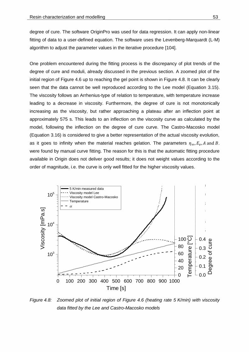
Resin characterization and modelling 53
degree of cure. The software OriginPro was used for data regression. It can apply non-linear
fitting of data to a user-defined equation. The software uses the Levenberg-Marquardt (L-M)
algorithm to adjust the parameter values in the iterative procedure [104].
One problem encountered during the fitting process is the discrepancy of plot trends of the
degree of cure and moduli, already discussed in the previous section. A zoomed plot of the
initial region of Figure 4.6 up to reaching the gel point is shown in Figure 4.8. It can be clearly
seen that the data cannot be well reproduced according to the Lee model (Equation 3.15).
The viscosity follows an Arrhenius-type of relation to temperature, with temperature increase
leading to a decrease in viscosity. Furthermore, the degree of cure is not monotonically
increasing as the viscosity, but rather approaching a plateau after an inflection point at
approximately 575 s. This leads to an inflection on the viscosity curve as calculated by the
model, following the inflection on the degree of cure curve. The Castro-Macosko model
(Equation 3.16) is considered to give a better representation of the actual viscosity evolution,
as it goes to infinity when the material reaches gelation. The parameters 𝜂∞, 𝐸𝑣 , 𝐴 and 𝐵.
were found by manual curve fitting. The reason for this is that the automatic fitting procedure
available in Origin does not deliver good results; it does not weight values according to the
order of magnitude, i.e. the curve is only well fitted for the higher viscosity values.
Figure 4.8: Zoomed plot of initial region of Figure 4.6 (heating rate 5 K/min) with viscosity
data fitted by the Lee and Castro-Macosko models
0 100 200 300 400 500 600 700 800 900 1000
103
104
105
Vis
cosity [m
Pa.s
]
Time [s]
5 K/min measured data
Viscosity model Lee
Viscosity model Castro-Macosko
Temperature
0
20
40
60
80
100
120
140
160
180
200
220
240T
em
pera
ture
[°C
]
0.0
0.1
0.2
0.3
0.4
0.5
0.6
0.7
0.8
0.9
1.0
Degre
e o
f cure

54 Resin characterization and modelling
The same curve behavior was observed in the measurements at the lower heating rate. The
fitting procedure was done the same way according to the Castro-Macosko model. The final
fitted parameters were found by averaging the parameters obtained for the two heating rates.
Figure 4.9 shows curves for both measured heating rates together with curves obtained from
the model according to the fitted parameters shown in Table 4.5. The model fits the viscosity
evolution obtained from both heating rates reasonably well. A probable cause for the
discrepancy might be the difference in mass of DSC and rheology samples. The relatively
large amount of material subjected to a measurement in the rheometer may have a possibly
inhomogeneous temperature distribution across the profile thickness. This would lead to an
onset of reaction at the surface layer, while the bulk of the material is still heating up, thus
leading to a more pronounced viscosity drop prior to curing. For the lower heating rate, the
effect is opposite; a self-acceleration process in the bulk of the material might already take
place, leading to a faster curing than predicted by the surface temperature.
Figure 4.9: Fitted viscosity curves for all heating rates
Table 4.5: Fitted parameters of Castro-Macosko viscosity model (Equation 3.16)
𝜂∞ [Pa·s] 𝐸𝑣 [J/mol] 𝛼𝑔 𝐴 𝐵
8 x 10⁻⁸ 56750 0.25 4.65 -10.5
0 500 1000 1500 2000 2500 3000 3500
103
104
105
106
107
Vis
cosity [m
Pa.s
]
Time [s]
1 K/min measured data
1 K/min model
5 K/min measured data
5 K/min model

Fiber characterization and modelling 55
5 Fiber characterization and modelling
To get a better estimate of input parameters for the process simulations, methods for
characterizing the fiber reinforcements employed in pultrusion were developed and tested in
this study. Most literature dealing with simulation of the pultrusion process have used
theoretical models for the estimation of permeability, e.g. from Kozeny-Carman or Gebart.
These models were fitted to the materials under study to assess their accuracy.
5.1 Material and methods
A description of the different fiber reinforcement materials tested is given in this section.
Subsequently, the testing molds and the testing procedure developed in this work are
described.
5.1.1 Reinforcement materials
The following reinforcements were characterized in terms of compressibility:
Glass fiber (GF) direct rovings 399A-AE, 4.800 tex (3B Company, Belgium)
Carbon fiber (CF) rovings Sigrafil C30, 50k (SGL Group, Meitingen, Germany)
Glass Continuous Filament Mat (CFM) 300 g/m² M8643 (3B Company)
Glass Continuous Strand Mat (CSM) 300 g/m² Conformat N720 (Superior Fibers, LLC,
Ohio, US)
Measurements were also performed on reinforcements layers wetted out with silicone oil
(Korasilon® M 1000, Kurt Obermeier GmbH & Co. KG, Germany) with a dynamic viscosity of
about 1 Pa·s at room temperature as soaking fluid. This value is within the range of
viscosities of typical resin formulations used in pultrusion.
The same glass and carbon fiber rovings were characterized in terms of their permeability.
Measurements were also conducted on CFM M8643 stacks. Silicone oil (Korasilon® M 100)
with a dynamic viscosity of about 0,1 Pa·s at room temperature was used as permeating
fluid.
The glass and carbon fiber rovings have coincidentally similar theoretical fiber volume
content on a roving basis, in spite of the different densities, linear weight (usually given in
tex, i.e. g/km) and fiber counts. The fiber volume content of a cross section filled with rovings
is given by the following equation:

56 Fiber characterization and modelling
𝑉𝑓 =
𝑁𝑅 ∙ 𝐿𝑊
𝐴 ∙ 𝜌𝑓 Equation 5.1
Where 𝑁𝑅 is the number of rovings and 𝐿𝑊 is the linear weight. The nominal and real values
for the rovings tested are given in Table 5.1. The values of linear weight were measured by
weighting of roving samples of 5 m in length. Six repetitions were performed for three
different rovings of the same lot.
Table 5.1: Nominal and real values of linear weight and rovings tested in this study
Nominal values Real values
Roving type 𝜌𝑓 [kg/m³] 𝐿𝑊 [tex] 𝐿𝑊 𝜌𝑓⁄
[x10-6 m²] 𝐿𝑊 [tex]
𝐿𝑊 𝜌𝑓⁄
[x10-6 m²]
3B 399A-AE 2620 4800 1.832 4910 1.874
SGL Sigrafil C30 50k 1800 3300 1.833 3322 1.845
The different types of mats have the same main function of providing strength perpendicular
to the pultruded product longitudinal direction. The Conformat N720 is also marketed as a
mat providing a better surface smoothness. The two mats exhibit a different appearance,
despite having the same area weight. The area weight tolerance was given at ± 10%.
However, a much lower discrepancy (± 3%) was found from several weighted pieces cut from
the same roll.
5.1.2 Compressibility method
Knowing the compressibility of pultrusion reinforcements is especially important when
designing a lay-up sequence for a pultrusion laminate. Many standard pultrusion profiles are
composed of stacked sequences of CFM and roving layers. Each layer has a different fiber
volume content, which is in part a function of the intrinsic fiber compressibility. Figure 5.1
shows this condition. For a given cross section thickness S, one (or more) CFM layer(s) with
thickness SM is a constituent of the profile. For the remaining cross section, a number of
rovings (thickness SR) must be chosen in order to achieve a profile with desirable mechanical
properties and easy processability. The pressure P is the force per unit area needed to
compress the fiber package to the geometrical constraint of the cross section given by the
pultrusion die. The fiber volume fraction in each of the layers is a function of the mechanical
pressure P and, in the case of multiple reinforcements, of the extent of the so-called nesting
effect, which is understood as the intertwining of adjacent layers into each other at their
interface.

Fiber characterization and modelling 57
Figure 5.1: Schematic representation of a laminate cross section composed of a CFM and
a roving layer
For measuring the compressibility, a mold with a cavity of 180 x 346 mm² was employed.
The mold has lateral shear edges and both ends open to the atmosphere. This allowed a
roving fiber stack to be positioned in a similar way as it would be in a pultrusion die, with the
individual rovings stretched and in the parallel orientation. The mold was mounted to a
universal testing machine.
The CFM layers were cut to cavity dimensions. Rovings were positioned by means of fixing a
polyethylene guiding plate with threading holes typically used in pultrusion processing trials.
The hole arrangement ensured a homogeneous distribution across the width of the cross
section. This was done by a lateral shifting between holes of a column according to the
pattern shown in Figure 5.2. This distribution is similar to patterns applied in the design of
guiding plates for actual pultrusion processing trials. Pictures of the mold assembly with
layers of rovings already in place are shown in Figure 5.3.
Figure 5.2: Hole pattern used in guiding plates for positioning of rovings in compressibility
measurements

58 Fiber characterization and modelling
(a) (b)
Figure 5.3: (a) Compressibility mold with glass fiber layer positioned for testing;
(b) Compressibility mold during testing of a carbon fiber layer
The load program was controlled at a displacement rate of 1 mm/min up to a maximum
compression load of 100 kN, which corresponds to 1.64 MPa compaction pressure. This was
followed by a time span of 5 min during which the position was held constant. The applied
force and corresponding displacement data were recorded. An example of a load-
displacement curve is shown in Figure 5.4.
Figure 5.4: Example of curve load vs. displacement obtained from the compression
measurement of a fiber roving fiber stack
0 100 200 300 400 500 600
0
2
4
6
8
10
Com
pre
ssio
n F
orc
e [x10
4 N
]
Time [s]
Compression Force
Position
-6
-5
-4
-3
-2
-1
0
Positio
n [m
m]

Fiber characterization and modelling 59
The compliance of the assembly composed of the mold and testing machine was determined
by performing a measurement without any reinforcement material. It was found that the mold
deflected 0.84 mm at a compression load of 100 kN relative to its closed position without
load. The real mold gap was then calculated by adding the displacement curve with
reinforcement material and the mold compliance curve. The fiber volume content was
obtained by using Equation 5.1 and substituting the cross section 𝐴 by the mold width and
the measured gap. The compaction pressure was obtained by dividing the compression load
by the mold surface area. At least two repetitions by compacting new material were
performed for each condition. Reproducibility was in general very good. In cases of deviating
curves, a third measurement was performed. The stress relaxation behavior under constant
displacement discernible in fiber reinforcements (see Figure 5.4) [62] was not included in this
analysis.
5.1.3 Permeability method
The permeability of fiber reinforcements is the most important parameter for simulating fluid
flow in composite processes. Most experimental studies on in-plane permeability have used
cells designed for measuring reinforcements typically used in RTM (e.g. fabrics, non-crimp
fabrics). Published studies focusing on flow simulation in pultrusion dies have usually applied
a permeability value calculated from a theoretical model (see Section 3.3.2). To validate this
assumption for reinforcement layers used in pultrusion processing, a method was developed
for the experimental estimation of the permeability of a reinforcement stack in which the
arrangement of rovings is similar to the processing configuration.
The mold for measuring the permeability had a cavity of 396 x 396 mm² and a central
injection nozzle. The mold was made of steel to avoid deflections (and consequently local
volume content variations), especially when applying the relatively high compaction
pressures common in pultrusion. The mold was analogous to the compressibility mold, i.e.
has shear edges for positioning and testing of a roving layer, and it was mounted to a
universal testing machine. The rovings were also positioned by means of guiding plates with
the same hole pattern shown in Figure 5.2.
For the permeability measurements, the cavity thickness was fixed by placing a stack of steel
strips of defined thickness (distancing shims) laterally between the mold halves. The mold
was then closed with the reinforcement material inside, such that the upper mold half
(approximate weight 185 kg) prevented the material from shifting. When measuring a roving
layer, the reinforcement stack was tensioned by means of clamping bars which were then

60 Fiber characterization and modelling
pulled away from the mold. Directly thereafter, a hole was cut through the reinforcement by a
punching tool with diameter 10 mm directly over the outlet of the central injection nozzle. The
central injection hole cut through the reinforcement was necessary to avoid flow gradients
through the thickness. The testing machine then pressed the two mold halves until the
distancing stack can no longer be moved, thus setting the cavity thickness. This preparation
sequence is shown in Figure 5.5. The procedure gave excellent cutting results for CFM,
fabrics and roving stacks, as seen in Figure 5.6.
Figure 5.5: Procedure for punching a central hole through the reinforcement stack before
infiltration
(a) (b) (c)
Figure 5.6: Cutting result into a roving fiber stack: (a) stack as seen from the top opening of
the mold before cutting; (b) punching tool being lifted after cutting; (c) stack
after cutting
Silicone oil was injected with constant pressure through the nozzle. Injection under constant
pressure was achieved by a pressurized pot. The flow front was detected when reaching
pressure transducers located at different positions within the cavity. Ten transducers were
mounted to the mold. Pictures of the open mold are shown in Figure 5.7. The fluid was
drained to a circular groove which defined the actual measurement cell as a circle with a
diameter of 350 mm.

Fiber characterization and modelling 61
(a) (b)
Figure 5.7: Permeability measurement cell: (a) open mold showing rovings guiding plate
and side metal strips for fixing the cavity thickness; (b) top view of mold
showing position of pressure transducer
The special sensitivity of the flow front detection method was previously assessed by
comparing visual flow and transducer response, and was determined to be below 2 mm. This
was the distance past the transducer location covered by the flow front when a pressure
increase was detected [105].
5.1.3.1 Unsaturated flow condition
The suitability of the measurement mold and method was assessed by measuring the same
glass fabric (Hexcel 01113) tested in a recent benchmarking exercise [64]. The analysis
proposed by Weitzenböck et al [70] was employed to obtain the principal permeability
parameters in-plane 𝐾1 and 𝐾2, as well as the angle between the principal permeabilities and
the axes of the coordinate system for unsaturated flow. The values found for 𝐾1
(approximately 8 x 10-11 m²) and 𝐾2 (approximately 2 x 10-11 m²) were within the range of
values reported in the benchmark, thus validating the developed mold and method [106].
The permeability of CFM was measured for fiber contents of 17.1%, 21.9% and 24.1% vol.
The fiber volume contents were chosen according to a compaction pressure range typically
processed in pultrusion (7 x 10⁴ – 4 x 10⁵ Pa). The material was cut from the roll to the mold
dimensions and stacked to four pieces. The orientation relative to the roll was kept constant
when stacking and laying into the mold (see Figure 5.13). A total of ten measurements were
performed for each fiber volume. The injection pressure was set to 6 bar.

62 Fiber characterization and modelling
5.1.3.2 Saturated flow condition
To analyze measurement data according to the Weitzenböck method, it is necessary that at
least one of the pressure sensors in the crosswise direction (P7 in Figure 5.7 (b)) is reached
before reaching the last sensor in the longitudinal direction (P3). In this particular
measurement cell, this means that data regression from unsaturated measurements is only
possible if a maximum difference of one order of magnitude exists between 𝐾1 and 𝐾2. This
was not the case observed when measuring unidirectional roving layers.
Rovings were measured for the fiber volume contents listed in Table 5.5, defined by the
adjusted cavity thickness. 300 roving ends were placed in the mold as shown in Figure 5.8.
Compaction forces between 120 – 200 kN were applied to close the mold, depending on
fiber volume content. The injection pressure was set to 1 bar for flow front measurements in
the unsaturated state and then increased to up to 6 bar for saturated flow measurements.
The inlet pressure was maintained until the system reached the steady state, i.e., no more
pressure changes occurred.
Figure 5.8: Permeability mold with carbon fiber roving stack
A recurrent problem faced during measurements of roving stacks was that individual rovings
which were cut (see Figure 5.6) shifted in position due to exerted fluid pressure. This effect
narrowed the possible measurement window on rovings with this technique to approximately
the range shown in Table 5.5. Shifting can be clearly detected during the measurement by an
increase of pressure signals along the rovings in the longitudinal direction (P1, P2 and P3),
and visually observed after the measurement. The effect was more intense when measuring
stacks of carbon fiber rovings.
Regression of data from saturated measurements was executed by means of a procedure
similar to that proposed by Arbter [72]. The absolute pressure values at different positions in

Fiber characterization and modelling 63
the cavity were used to determine the permeability in a saturated flow condition, i.e. in the
equilibrium state. In order to find the permeability parameters, the steady-state flow was
simulated in CFD software (Ansys CFX). The simulation model is shown in Figure 5.9.
Figure 5.9: Simulation model for calculation of permeability parameters in saturated state
Initial permeability parameters were set as the initial values and the corresponding pressure
field was then calculated. An optimization function was implemented to find 𝐾1 and 𝐾2. The
optimization function varied the values of 𝐾1 and 𝐾2 within a defined range and evaluated
the minimum of the sum of squared residuals between three measured and simulated
pressure values located in the principal axes 𝑥 and 𝑦, and at an angle of 45° to the principal
axes. Unless otherwise noted, the measured values of 𝑃3, 𝑃4 and 𝑃7 were taken as input
values for the optimization function. The residual function was given by:
𝑃𝑅 = 𝑚𝑖𝑛 [1
3√(
𝑃3,𝑠 − 𝑃3,𝑚
𝑃3,𝑚)
2
+ (𝑃4,𝑠 − 𝑃4,𝑚
𝑃4,𝑚)
2
+ (𝑃7,𝑠 − 𝑃7,𝑚
𝑃7,𝑚)
2
] Equation 5.2
where the subscripts 𝑚 and 𝑠 denote measured and simulated values respectively. The
optimization function minimized the averaged relative error between all pressure values
measured and simulated. It was assumed that the directions of the principal permeabilities
coincide with the reference axes, i.e. of 𝐾1 = 𝐾𝑥, 𝐾2 = 𝐾𝑦. This was a necessary assumption
for this calculation method, and it was considered reasonable for a unidirectional fiber stack.

64 Fiber characterization and modelling
5.2 Compressibility measurement results
Measurements on rovings were performed in three different roving counts to evaluate the
effect of the overall layer thickness on the compression behavior. Measurements on CFMs
were performed on single and double layers to assess if a significant nesting effect could be
detected. A mat/roving/mat laminate structure typically processed in pultrusion was tested to
evaluate potential nesting effects. A list of the conducted tests is shown in Table 5.2. Curves
of compaction pressure vs. fiber volume content for glass and carbon fiber roving layers are
shown in Figure 5.10.
Table 5.2: Reinforcement layers configurations tested for their compressibility
Type of reinforcement Number of specimens Sample condition
GF Rovings 80 / 120 / 160 Dry
CF Rovings 80 / 120 / 160 Dry
CFM M8643 1 / 2 Dry / wetted out
CSM N720 1 / 2 Dry / wetted out
CFM - GF Rovings - CFM 1 - 80 - 1 Dry / wetted out
CSM - GF Rovings - CSM 1 - 80 - 1 Dry / wetted out
Figure 5.10: Curves of pressure vs. fiber volume content for fiber stacks composed of glass
(GF) and carbon (CF) fiber rovings with different fiber counts
0.30 0.35 0.40 0.45 0.50 0.55 0.60 0.65 0.70
0
2
4
6
8
10
12
14
16
Pre
ssure
[x10
5 P
a]
Vf
CF 80 Rovings
CF 120 Rovings
CF 160 Rovings
GF 80 Rovings
GF 120 Rovings
GF 160 Rovings

Fiber characterization and modelling 65
The compression behavior of rovings can be described as relatively insensitive to variations
in the applied mechanical pressure, i.e. the stack is rather incompressible. This is due to the
fact that fibers are already in a parallel orientation. A small variation in the number of rovings
ends being fed to the pultrusion die can have a significant impact on processing stability.
This implies that adding or removing a few rovings will have a significant impact on the
mechanical pressure exerted by the die over the fiber stack. If the fiber volume content is too
low, resin deposition is likely to occur in the die, if it is too high, pulling the bundle through the
die will not be possible.
The compressibility of the roving stack was found to be dependent on the roving count. A
larger number of rovings resulted in a higher fiber volume content for the same compression
pressure applied. This was valid for both glass and carbon fibers. This can be explained by
an increasing nesting effect of fibers intertwining within each other as the fiber stack gap
increased.
The carbon fiber rovings were found to be more compressible and reach higher fiber volume
content than glass fiber stacks for the same compaction pressure. This is probably due to
different material conditioning and packaging. Carbon fibers are delivered twistless and
spread-wound in cardboard rolls; glass fiber rovings, on the other hand, are delivered in
packages from which the roving is pulled from the inside. This inevitably brings a periodic
twist along the roving length. The carbon fiber filaments thus have a more parallel orientation
within the roving, allowing for increased compaction.
Experimental data was fitted by the model proposed by Gutowski [61] (Equation 3.17). The
values shown in Table 5.3 were used to calculate the bending stiffness of glass and carbon
fibers. A value of 0.35 was used for 𝑉0 in all cases. The fitted parameters 𝛽 and 𝑉𝑎 are shown
in Table 5.4.
Table 5.3: Material parameters and calculated bending stiffness of fibers
Carbon fiber Glass fiber
Young’s modulus [Pa] 2.4 x 10¹¹ 8.2 x 10¹⁰
Filament diameter [µm] 7 24
Area moment of inertia [mm4] 1.89 x 10⁻⁹ 2.61 x 10⁻⁷
Bending stiffness [N.m²] 4.53 x 10⁻¹⁰ 2.14 x 10⁻⁸

66 Fiber characterization and modelling
Table 5.4: Fitted parameters for roving fiber stacks according to the Gutowski’s model
Roving count
𝛽 [mm] 𝑉0 𝑉𝑎 𝑅2
Carbon fiber stack
80 1.08 0.35 0.880 0.999
120 1.27 0.35 0.878 0.997
160 1.32 0.35 0.877 0.999
Glass fiber stack
80 2.54 0.35 0.871 0.998
120 2.81 0.35 0.872 0.989
160 3.09 0.35 0.872 0.996
CFM 3B M8634 - 0.80 0.10 0.977 0.999
CSM SF N720 - 0.03 0.05 89.57 0.999
The correlation coefficient values 𝑅2 indicated that a good fit was obtained in all cases. In
fact, good fitting results can be obtained for a range of pair values of 𝛽 and 𝑉𝑎. The values
shown in Table 5.4 were obtained by setting 𝑉𝑎 to a narrow range while 𝛽 was fitted.
According to the theoretical framework proposed by Gutowski, the model assumes
transverse fiber rearrangement during compression. This could result in a higher maximum
possible fiber volume fraction 𝑉𝑎, or in a larger span length to span width ratio 𝛽. It is
reasonable to assume that both effects occur simultaneously; rearrangement of fibers during
compression may lead to changes in the packing distribution (between a square and a
hexagonal array). It also leads to changes in the density of available contact points or scale
of waviness within the beam network, which are described by the value 𝛽. According to this
reasoning, it is expected that compressibility will be affected by the compression speed
applied.
Constraining the value of 𝑉𝑎 is, therefore, an arbitrary decision, as was noted by Gutowski.
Nevertheless, it helps to evaluate the effect of roving count on the value of 𝛽. For a thicker
fiber stack, the bulk of the material will have more rearrangement freedom during
compression in comparison to a thinner fiber stack, thus resulting in a larger 𝛽. The values
also indicated a larger waviness of glass in comparison to carbon fiber stacks.
Curves of compaction pressure vs. fiber volume content for the random glass fiber mats are
shown in Figure 5.11. CFM and CSM, in contrast to roving layers, are generally more
compressible, i.e. a variation in compression has a more pronounced effect on the fiber
volume content in comparison to a roving layer. This property is effectively applied in
pultrusion processing to extend the processing window by balancing variations in the roving
layer. It is also noteworthy that the compressibility of the two apparently similar materials is

Fiber characterization and modelling 67
very different. The CFM from 3B reached a volume content of approximately 0.3 while the
CSM from Superior Fibers reached approximately 0.21 for the same maximum compaction
pressure of 1.64 MPa. The nesting effect was also more pronounced in the 3B CFM, as can
be seen by the difference between the curves for single and double layers.
Figure 5.11: Curves of pressure vs. fiber volume content for single and double layers of
glass fiber continuous mats
The fitting procedure was also applied to the mats. Fitted parameters are also shown in
Table 5.4. Since the goal was to obtain a straightforward procedure for determining a
reinforcement layup given the mechanical pressure and thickness, only the curves for single
layers of the two mats in dry condition were fitted. In the case of mats, setting a value of 𝑉𝑎
according to fiber packing makes little sense. Therefore, both 𝑉𝑎 and 𝛽 were fitted without
any range constraints.
The nesting effect present in a multilayer laminate can also be evaluated by comparing the
measured curve of laminate thickness (s) vs. compaction pressure (P) for a mat/roving/mat
stack and the added curves of the same layers (see Figure 5.12). Due to nesting, there will
be an error of about 5% – 10% in the cavity thickness (and consequently in the average fiber
volume content) when using the single curves of the materials to calculate the multilayer
laminate structure. In practical terms, a lower number of rovings will be determined than
actually needed to achieve the same laminate thickness at the given compaction pressure.
0.00 0.05 0.10 0.15 0.20 0.25 0.30 0.35
0
2
4
6
8
10
12
14
16
Vf
Pre
ssu
re [x1
05 P
a]
CFM 3B M8643 1x dry
CFM 3B M8643 2x dry
CFM 3B M8643 1x wetted out
CSM SF N720 1x dry
CSM SF N720 2x dry
CSM SF N720 1x wetted out

68 Fiber characterization and modelling
Figure 5.12: Curves of pressure vs. layer thickness for mat/roving/mat stacks
The effect of wetting out the reinforcement was also investigated. For low pressures (0 -
0.1 MPa), the curve for wetted reinforcement was close to the theoretical curve of added
layers. That means that at this pressure range, wetting-out of reinforcement compensated
the nesting effect. For the pressure range up to 0.6 MPa, the compressibility curves of the
wet-out and dry reinforcement became close to each other, as the compaction pressure
effectively squeezes out the soaking fluid. In this pressure range, the error incurred by
adding up the layers must be considered. It should be noted however, that a dependence
between profile structure and the deviations discussed above was expected, for example in
the case of a thick laminate (over 4 mm) in which more than 2 layers of CFM are present, or
when working with a resin of different viscosity.
When designing a reinforcement layup, one must know beforehand a suitable range of
mechanical pressure, which must be experimentally determined. According to experience
from pultrusion experiments in the pultrusion lab at Fraunhofer, typical compaction pressures
for a mat-roving-mat stack range from 0.5 to 4.0 bar. Higher pressures will cause tearing of
the mats [107]. As an example, for a compaction pressure of 2.4 bar and a laminate
thickness of 3.0 mm, a glass fiber roving layer would consist of 118 rovings, if the top and
bottom mats are 3B M8643, or 73 rovings in combination with SF N730 mat layers. This
calculation example illustrates the significant impact of the chosen reinforcement on the
layup design.
0 2 4 6 8 10 12 14 16
0.0
0.5
1.0
1.5
2.0
2.5
3.0
3.5
4.0
4.5
5.0
5.5
6.0
Thic
kness [m
m]
Pressure [x105 Pa]
Added 3B + 80 Rovings + 3B
Measured 3B + 80 Rovings + 3B dry
Measured 3B + 80 Rovings + 3B wetted out
Added SF + 80 Rovings + SF
Measured SF + 80 Rovings + SF dry
Measured SF + 80 Rovings + SF wetted out

Fiber characterization and modelling 69
5.3 Permeability measurement results
Results obtained from unsaturated flow measurements within CFM stacks and saturated flow
measurements within unidirectional roving stacks are presented in this section. The results
obtained from measurements on rovings are compared to predictions from a theoretical
model, and the validity and limitations of the developed characterization technique are
discussed.
5.3.1 Continuous filament mats
The permeability measurement results for the CFM stacks are shown in Figure 5.13.
Figure 5.13: Results of permeability measurements on CFM stacks. Top: permeability
parameters in the plane directions; bottom: calculated angle between the
principal permeabilities and the reference plane directions
It is interesting to note that with increasing fiber volume content, the accuracy of the
measurement clearly improves for both 𝐾1 and 𝐾2. One possible explanation for this behavior
might be the fact that for lower volume contents, the fluid flows not only through the bulk
region of the mats, but also to some extent between the mat and the mold walls. These local
variations may be suppressed when the fiber stack is subjected to a higher compaction
pressure, resulting in flow only through the porous material.
0.150 0.175 0.200 0.225 0.250 0.275
-10
0
10
Angle
K1 experimental
K2 experimental
K1 model
K2 model
Angle
[°]
Vf
2
4
6
8
10
12
14
K1 / K
2 [x10
-10 m
²]
Kozeny Constants
kc1
= 0,88254
kc2
= 0,66213

70 Fiber characterization and modelling
On the other hand, the scattering of the determined angle between the principal
permeabilities and coordinate system increased with increasing fiber volume content. This
might arise from the inherent fluctuation of specific weight in CFM materials. A specific
weight with ± 10% fluctuation is typically declared for this kind of material. These local
variations may result in scattering on the orientation of main permeabilities between the
measurements. In contrast to the general assumption that CFM is an isotropic material, a
subtle, though discernible anisotropic permeability was observed, with the permeability in the
transverse direction relative to the roll winding direction higher than in the parallel orientation.
The experimental data was fitted to the Kozeny-Carman model (Equation 3.19). The fiber
radius was set to 12 µm, a typical value of glass fibers. The fitted curves are shown in Figure
5.13. This allowed the prediction of the permeability of a CFM layer given a particular
laminate and compaction pressure. It must be stressed once again that these results are
intrinsic to the particular M8643 CFM material only.
5.3.2 Roving stacks
Measurements of roving stacks showed a higher degree of anisotropy than predicted by
models such as proposed by Gebart [74], and experimentally determined by Schell et al.
[78]. These studies presented, for a bundle of parallel oriented fibers, a difference between
the longitudinal and the transverse permeabilities of around one degree of magnitude. Such
a difference lies within the limits of the measurability by the method of Weitzenböck et al. [69]
and the mold configuration. Higher degrees of anisotropy, however, resulted in the testing
fluid reaching the third pressure transducer in the longitudinal direction before the first
transducer in the transverse direction. This flow behavior prevented an analysis of the
unsaturated flow condition.
For the saturated flow, it was necessary that a steady state was reached, in which the
pressure distribution over the measurement region no longer varied with time. Typical
pressure distributions such as shown in Figure 5.14 were obtained. It can be seen that a long
time was needed to reach steady state; after setting the pressure to 4,4 bar at the inlet, more
than 1.5 h were needed for the fluid to reach P7, and steady state was reached after 3.5 h.
The inlet pressure was then increased to 6.0 bar after 4.2 h of measurement, to obtain
another pressure distribution for the same fiber volume content.
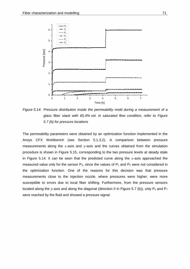
Fiber characterization and modelling 71
Figure 5.14: Pressure distribution inside the permeability mold during a measurement of a
glass fiber stack with 65,4% vol. in saturated flow condition, refer to Figure
5.7 (b) for pressure locations
The permeability parameters were obtained by an optimization function implemented in the
Ansys CFX Workbench (see Section 5.1.3.2). A comparison between pressure
measurements along the 𝑥-axis and 𝑦-axis and the curves obtained from the simulation
procedure is shown in Figure 5.15, corresponding to the two pressure levels at steady state
in Figure 5.14. It can be seen that the predicted curve along the 𝑥-axis approached the
measured value only for the sensor P3, since the values of P1 and P2 were not considered in
the optimization function. One of the reasons for this decision was that pressure
measurements close to the injection nozzle, where pressures were higher, were more
susceptible to errors due to local fiber shifting. Furthermore, from the pressure sensors
located along the 𝑦-axis and along the diagonal (direction II in Figure 5.7 (b)), only P4 and P7
were reached by the fluid and showed a pressure signal.
0 1 2 3 4 5 6 7
0
1
2
3
4
5
6
Pre
ssure
[bar]
Time [h]
P0
P1
P2
P3
P4
P7

72 Fiber characterization and modelling
Figure 5.15: Comparison between measured pressures and curves predicted by simulation
The results obtained are listed in Table 5.5. For the glass fiber stacks, six measurements
were evaluated for each fiber volume content. For each of them, the optimization procedure
was conducted to obtain a value of 𝐾1 and 𝐾2. The PR value shown is an average from the
residuals calculated in the optimization procedure. Measurements performed on carbon fiber
stacks showed no response from pressure sensor P7. The optimization was then conducted
using only the measured values of P3 and P4. For the 62,4% vol. case, only two
measurements led to a steady state and could be evaluated because of repeated fiber
shifting. Therefore, no standard deviation is shown for this measurement point. The results
were compared with the predicted permeabilities according to the Gebart’s model [74]
(Equation 3.19 and Equation 3.20). The results of the glass fiber stack measurements are
shown in Figure 5.16, and for carbon fiber stacks in Figure 5.17.
Table 5.5: Results of permeability measurements on roving stacks
𝑉𝑓 K1 [m²] K2 [m²] PR
Glass fiber stack 0.595 (4,8 ± 0,1) x 10-12 (5.4 ± 0,9) x 10-14 0,16
0.654 (2.4 ± 0.1) x 10-12 (2.5 ± 0,8) x 10-14 0,17
Carbon fiber stack
0.624 1.4 x 10⁻¹² 2,0 x 10⁻¹⁵ 0,13
0.655 (7,0 ± 3,9) x 10-13 (1.6 ± 0.6) x 10-15 0,24
0.00 0.05 0.10 0.15 0.20
0
1
2
3
4
5
6
P0
P1
P2
P3P7
Pre
ssu
re [b
ar]
Distance along x and y axes [m]
Pinlet
= 4,4 bar
P x axis, simulation
P y axis, simulation
Pressure measurements
Pinlet
= 6,0 bar
P x axis, simulation
P y axis, simulation
Pressure measurements
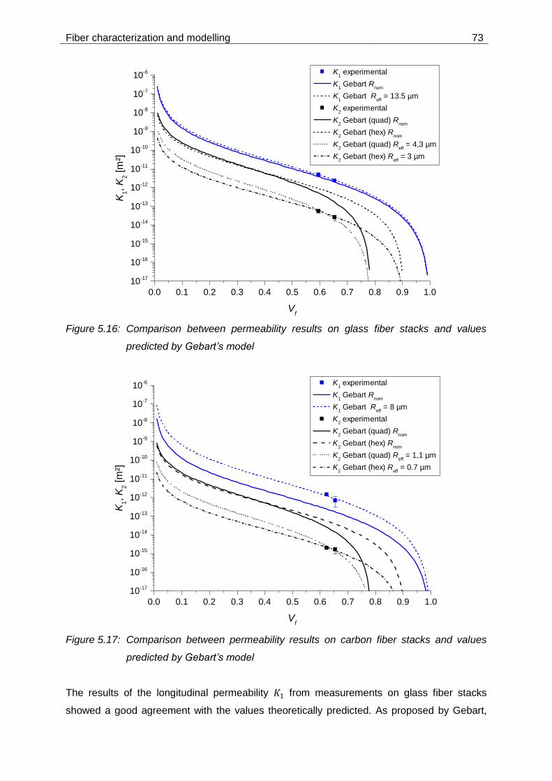
Fiber characterization and modelling 73
Figure 5.16: Comparison between permeability results on glass fiber stacks and values
predicted by Gebart’s model
Figure 5.17: Comparison between permeability results on carbon fiber stacks and values
predicted by Gebart’s model
The results of the longitudinal permeability 𝐾1 from measurements on glass fiber stacks
showed a good agreement with the values theoretically predicted. As proposed by Gebart,
0.0 0.1 0.2 0.3 0.4 0.5 0.6 0.7 0.8 0.9 1.0
10-17
10-16
10-15
10-14
10-13
10-12
10-11
10-10
10-9
10-8
10-7
10-6 K
1 experimental
K1 Gebart R
nom
K1 Gebart R
eff = 13.5 µm
K2 experimental
K2 Gebart (quad) R
nom
K2 Gebart (hex) R
nom
K2 Gebart (quad) R
eff = 4,3 µm
K2 Gebart (hex) R
eff = 3 µm
K1, K
2 [m
²]
Vf
0.0 0.1 0.2 0.3 0.4 0.5 0.6 0.7 0.8 0.9 1.0
10-17
10-16
10-15
10-14
10-13
10-12
10-11
10-10
10-9
10-8
10-7
10-6 K
1 experimental
K1 Gebart R
nom
K1 Gebart R
eff = 8 µm
K2 experimental
K2 Gebart (quad) R
nom
K2 Gebart (hex) R
nom
K2 Gebart (quad) R
eff = 1,1 µm
K2 Gebart (hex) R
eff = 0.7 µm
K1, K
2 [m
²]
Vf

74 Fiber characterization and modelling
an “effective fiber radius” was chosen to superpose the model curve to measured data. Only
a minor correction relatively to the nominal radius of 12 µm was needed for this case. The
discrepancy in the carbon fibers case was slightly larger. For the longitudinal permeability,
the measured permeability was higher than the model prediction for the carbon fiber nominal
radius of 3.5 µm.
For the transverse permeability, a much larger deviation of up to one order of magnitude
from the model was observed for the glass fibers. It should also be noted that, in the fiber
volume content region considered, the model predictions considering a quadratic and a
hexagonal fiber packing diverge from each other. This resulted in different effective fiber radii
needed to superpose model and measurement results and consequently in different
predicted values in the lower fiber volume region.
The large discrepancy in the transverse permeability might be due to an imperfect parallel
orientation of the fibers. Stacked rovings created regions with higher volume content, which
effectively prevented transverse flow. Twisting and undulations are characteristic and clearly
discernible in direct glass fiber rovings, which might contribute to obstruction of the flow.
Furthermore, these characteristics made a perfect stretching of the fibers more difficult,
accentuating the problem of fiber stacking. Nevertheless, the measurement assembly
reproduces to a large extent a typical configuration of a pultrusion die in-feed. The
experimental results obtained are thus considered to be representative of flow conditions
through a roving layer prevailing in pultrusion processing.
The method developed here has, nevertheless, limitations regarding the measurement of a
unidirectional fiber stack. The measurable fiber volume content region was very narrow
between a lower limit where fiber shifting in the cut region is unavoidable, and an upper limit
where no pressure is detected in the direction transverse to the fiber orientation. The
extrapolation of results to lower fiber volume fractions shown in Figure 5.16 and Figure 5.17
should, therefore, be considered with caution. The method was time-consuming due to the
large amount of rovings threaded prior to each measurement. Furthermore, an analytic
solution would be preferred over the optimization approach, e.g. according to the method
proposed by Han et al [71], which was not possible with the method and material considered
due to the very low volumetric flow rate of the permeating fluid. The analytic solution would
allow a proper error propagation analysis and therefore a strict quantitative evaluation of the
method. In the presented stage of development, the method is only suitable for a qualitative
assessment of permeability.

Experimental trials with closed injection dies 75
6 Experimental trials with closed injection dies
To compare experimental data to processing simulation results, a series of trials was
conducted using two pultrusion dies with closed injection and impregnation chambers. One
of the dies had a design based on the description contained in Brown’s patent [8]. This die
design is referred to as conical. The other die had a design according to Koppernaes [6] and
is referred to in this study as tear drop.
The pultrusion machine used for the trials was a model Px500-10T (Pultrex Ltd., Essex, UK),
corresponding to the current state of the art. The pulling device consisted of a pair of
alternating pullers. Each puller was fixed to a linear track and coupled to an electro-
mechanical gear based on a ball screw mechanism, which could precisely control the linear
speed. The hub of each puller was approximately 50 cm. The material being processed was
pulled by one of the pullers until close to the end of the hub, when the second puller then
clamped the profile and traveled at the same speed of the first one until the latter one
reached the end of the hub and released the profile.
The mixing and metering machine (model type Nodopur VS, Tartler GmbH, Michelstadt,
Germany) was a system designed for processing of two-component polyurethane resins of
low to medium viscosity. The system had two separate tanks for storing the two resin
components. The metering was done by gear pumps with volume flow meters at their
discharges. The pump throughput was continuously controlled by a proportional–integral–
derivative (PID) controller according to the measured volume flow. Gear pumps have the
advantages of very precise metering and of pumping constant throughputs regardless of the
counter-pressure at the discharge (up to a certain limit given by the gear motor).
Trials were conducted with each die by processing unidirectional fiber stacks composed of
carbon and of glass fiber rovings. Rovings processed were the same grades characterized in
Section 5, i.e. glass fiber direct rovings 399A-AE 4.800 tex and carbon fiber rovings Sigrafil
C30 50k. The resin formulation processed was the same described in Section 4, that is, the
Daron ZW 015864 resin formulated with curing agent, catalysts and processing additives.
The die was heated by means of electrical heating plates. The temperatures were controlled
by thermocouples located in the die body, drilled close to the inner cavity. Processing
temperatures were adjusted to partially cure the material to reach a B-stage condition in the
pultrusion die. The set temperature was equal for all heating zones in a particular trial.

76 Experimental trials with closed injection dies
The processing parameters varied were the pulling speed and fiber volume content.
Processing data recorded throughout the trial included:
Pulling speed (real time speed)
Pulling force
Temperature at different positions along the length of the metal die
Power input to the electrical heaters (percentage value of nominal output)
Pressure in the liquid region of the die
Pressures at the discharge of the resin mixing and metering unit (injection pressure)
Resin mass flow rate
Additionally, the temperature within the processed material was measured by letting a wire
thermocouple to be pulled together with the fiber bundle over the entire die length. This
allowed for getting a temperature profile as the resin (partially) cures along the die. A
summary of the conducted trials is presented in Table 6.1.
Table 6.1: Summary of conducted pultrusion processing trials
Trial number
1 2 3 4 5 6 7 8 9 10
Pultrusion die * C C C C C C TD TD TD TD
Fiber stack ** GF GF GF CF CF CF GF GF GF GF
Pulling speed [m/min] 0.3 0.3 0.3 0.5 0.3 0.3 0.5 0.3 0.3 0.3
Fiber volume content [%] 0.64 0.6 0.57 0.64 0.64 0.6 0.64 0.64 0.6 0.64
Set Temperature [°C] 100 100 100 100 100 100 100 100 100 80
* C = conical; TD = Tear Drop
** GF = glass fibers; CF = carbon fibers.
6.1 Description of trial assemblies
In this section, both dies applied during the experimental trials are presented, in terms of
their working principle, mechanical assembly, temperature management by means of cooling
and heating plates, and integration of temperature and pressure sensors. Their similarities
and differences related to processing are also briefly described.

Experimental trials with closed injection dies 77
6.1.1 Conical die
The pultrusion die with conical injection and impregnation chamber consisted in fact of a
standard die, i.e. a die with a straight inner cavity of constant cross section, in this case a flat
sheet of 90.0 x 4.0 mm². The die length was 1220 mm. The conical injection chamber is
mechanically aligned and fixed to the main die. The chamber had 500 mm of length, and a
tapering angle of 1°. A guiding plate was bolted directly to the inlet of the injection chamber.
Its primary function was to uniformly distribute the rovings over the cross section. By
separating them, it also facilitated flowing of resin between rovings in the cross-wise
direction. The resin formulation was injected through four nozzles (two located each at the
top and bottom) at a distance of 200 mm from the chamber inlet. An opening to the
atmosphere located at 110 mm from the chamber inlet (center, opening length 50 mm)
allowed for observation of the flow front. This design had proven to give good results on the
processing of reinforcements stacks consisting of rovings only. A schematic representation of
the die assembly is shown in Figure 6.1.
Figure 6.1: Schematic representation of die assembly with conical inlet geometry
A particular advantage of this design over the tear drop is that no stagnation regions with
long resin residence time are formed. On the other hand, processing of profiles with more
complex reinforcement layups may be more challenging, depending on the type of
reinforcements and stacking sequence [1].
Two pressure sensors (Dynisco SPX2292, measurement range 0 – 70 bar) were located
near the end of the conical section and at the beginning of the straight section. These
sensors had a relatively large membrane surface (diameter of approximately 23.5 mm) and
are thus appropriate to measure an average pressure while in contact with the fiber stack.
A total of eleven thermocouples measured the temperatures along the die. Four of these
were used as control values for the set temperatures in four heating zones located along the

78 Experimental trials with closed injection dies
die main body (TC1 to TC4). Each heating zone consisted of one electrical heater fixed at
the top and one at the bottom of the die. The nominal power of heating cartridges in each
plate was 1000 W, and the contact area was 200 x 80 mm². A pair of cooling plates was fixed
at the top and bottom at the junction between the tapered chamber and the straight die. The
die and the injection chamber did not have the same thickness, therefore the contact length
of the cooling plates was reduced (see Figure 6.1).
6.1.2 Tear drop die
The die with tear drop geometry evaluated in the trials was designed and manufactured as a
die specific for closed injection pultrusion, i.e. the injection and curing sections are milled
from a single piece of tool steel. The inner cavity in the straight section had dimensions of
180 x 2.45 mm². The inlet had a length of 100 mm and the same cross section as the curing
section. It was followed by a conically constraining injection and impregnation region with
320 mm length and tapering angle of 1.2°. This corresponded to a maximum cavity height of
8.0 mm at the position 116 mm (distance from die inlet), where the resin was injected.
Injection was done through three nozzles at the bottom and another three nozzles
symmetrically arranged at the top side of the die. The total die length was 1318 mm. A
guiding plate was also used for positioning the rovings prior to entering the die; however, it
was not attached to the die as in the conical die assembly, but fixed at a distance of about
400 mm from the die inlet. The hole configuration was like the sketch shown in Figure 5.2.
As stated previously, this die design is susceptible to stagnation regions with long resin
residence times. Stable operation over several hours is highly dependent on a proper die
design which avoids such stagnation region and at the same time assures thorough wetting
out of reinforcements. Furthermore, it is dependent on resin reactivity. This design was found
to be suitable for processing of standard resin formulations with long pot life at room
temperature such as vinyl ester [12].
Similarly to the conical die, pressure transducers were mounted in the die, located near the
resin injection points and at the beginning of the straight curing section. During operation, the
pressure value at the first transducer was an important monitoring parameter that indicated
whether the chamber was full of liquid material. To ensure that the chamber was full at all
times, the flow rate was adjusted such that an excess of resin flowed out of the die inlet.
Nine thermocouples measured the temperatures along the die. Three of these were used as
control values for the set temperatures in three heating zones located along the die main

Experimental trials with closed injection dies 79
body (TC1 to TC3). Each heating zone consisted of two electrical heaters (same type
employed for the conical die) fixed side by side at the top and two at the bottom of the die. A
pair of cooling plates was fixed at the top and bottom at the end of the tapered section. A
sketch of the trial assembly is shown in Figure 6.2.
Figure 6.2: Schematic representation of die assembly with tear drop inlet geometry
6.2 Experimental data
Examples of processing data obtained from the experimental trials with both dies are
presented and analyzed in terms of their significance to processing in this section. Qualitative
correlation between processing parameters is also discussed. The focus is given to data
relevant for comparison and validation of the simulation studies conducted in Section 7.2. A
summary of data obtained for the different trial configurations (see Table 6.1) is given in
Appendix A.
6.2.1 Conical die
Temperature profiles along the die are shown for the trial configuration 1 (see Table 6.1) in
Figure 6.3. The exothermic heat generated by the B-staging reaction leads to an increase in
temperature above the set temperature of the heating zones up to approximately 115 °C
between heating zones 1 and 2. This can be observed both by the signals of the wire
thermocouples as well by the value of the monitoring thermocouple located at the x-position
870 mm. A slight difference in the temperature development can also be seen between the
profile center and surface. By comparing both curves, one can conclude that the overall
reaction heat generation is moderate; otherwise, an increase in the center temperature
above that of the surface would be observed.

80 Experimental trials with closed injection dies
Figure 6.3: Temperature profiles in the conical die assembly (trial configuration 1) obtained
from wire thermocouples fed through the die and from thermocouples
positioned in the die
No significant difference in the temperature profiles was observed when processing carbon
fiber rovings instead of glass fibers. Variations of fiber volume content did not result in
differences in the temperature profiles either. By increasing the pulling speed to 0.5 m/min, a
lateral shifting of the curves along the x-position took place, while the maximum temperature
reached remained at a similar level.
During all trials, no completion of the reaction to a fully cured material was observed.
Whether the temperature development led to an incipient radical polymerization cannot be
determined from the experimental trials and product appearance alone. According to the
prediction shown in Figure 4.4, the second reaction step initiates after approximately 5 min at
a constant temperature of 120 °C. However, the prediction by the Thermokinetics software
does not take into account the mass and local temperature increase in the material. A spatial
or volumetric simulation is expected to give a better estimation of the real material state by
the end of the pultrusion process in this case.
The individual temperatures of the control and monitoring thermocouples were kept stable at
the values shown in Figure 6.3. This was due to the high specific heat capacity of steel. The
power input to the electrical heaters is logged by the machine as a percentage of the nominal
heater power. These values are shown in Figure 6.4 as an example for the same time span
0 250 500 750 1000 1250 1500 1750
20
30
40
50
60
70
80
90
100
110
120
130
Tem
pera
ture
[°C
]
x-position from die inlet [mm]
TC profile surface
TC profile center
Control TC
Monitoring TC

Experimental trials with closed injection dies 81
of 20 min during which the data shown in Figure 6.3 was obtained. The signals of the
thermocouples 1 through 6 are also plotted.
The temperatures of the control zones were constant at approximately 100 °C at all zones,
and the temperatures of the thermocouples 5 (located at the injection chamber) and 6
(exothermic peak located after the thermocouple 1) were also at a constant level. The power
input values, on the other hand, varied over time. The calculated average values over the
time span are indicated in the graph. The heat needed to trigger the reaction was transferred
solely by zone 1. Zone 2 was only sporadically turned on, which was due to the heat
generated by the reaction and subsequent heat build-up between zones 1 and 2. Towards
the downstream portion of the die, zones 3 and 4 were again contributing with a net heat
input to maintain the set temperature after the exothermic reaction heat generation had
subsided.
Figure 6.4: Thermocouple signals and power input to the electrical heaters over a 20 min
time span during trial configuration 1
The signals of measured pulling force, pulling speed and liquid pressures are shown in
Figure 6.5. In contrast to the temperature signals, these processing parameters undergo to
some extent strong variations over time, in particular the pulling force and the pressure
transducer 2 (located at the beginning of the straight die section). In comparison, the
pressure measured by the transducer 1 (in the tapered die inlet) showed smaller absolute
variations, although the perceptual variation of all signals lied around 10%. The resin was
09:55 10:00 10:05 10:10 10:15
0
20
40
60
80
100
120
Tem
pera
ture
[°C
]
Time [h:min]
TC01
TC02
TC03
TC04
TC05
TC06
0
20
40
60
80
100
Average values [%]
Electrical Power, Zone 1 46,0 5,9
Electrical Power, Zone 2 1,4 2,9
Electrical Power, Zone 3 7,2 3,9
Electrical Power, Zone 4 12,8 5,6
Ele
ctr
ical pow
er
[%]

82 Experimental trials with closed injection dies
injected at a low pressure (0.4 bar). An injection pressure was only recorded when the
metering unit was pumping resin. The injection was thus intermittent, because the minimum
flow rate was too large relatively to the throughput needed for the specific combination of die
cavity, fiber content and pulling speed.
Figure 6.5: Plots of measured pulling force, pulling speed and liquid resin pressures over a
20 min time span during trial configuration 1
Short drops in the pulling speed occurred periodically, which also caused corresponding
drops in the pulling force and pressure signals. This is due to the pulling mechanism
composed of alternating pullers, and is related to the handover of one puller to the other.
Furthermore, a correlation existed between the level of pulling force and the pressures
measured in the liquid region, especially the peak pressure at the conical-straight transition
region. This suggests that the pulling resistance in the processing trials was caused, to a
considerable amount, by the pressure of liquid resin over the die walls, which can be
expressed by Equation 3.33.
The large variations observed in the signals in Figure 6.5 are to some extent caused by the
intermittent injection. The resin injection was manually turned on and off, by observing the
flow front position at the opening to the atmosphere. The variation in the flow front position
could already cause a pressure variation. Another hypothesis for the fluctuations could be a
deformation of the die inner cavity due to the high pressures developed in the process. With
increasing pressure, the deformation would be accentuated in terms of cavity expansion,
09:55 10:00 10:05 10:10 10:15
0
2
4
6
8
10
12
14
16
18
20
Pulli
ng forc
e [kN
]
Time [h:min]
Average values
Pulling force (12,1 1,5) kN
Pressure transducer 1 (8,9 0,9) bar
Pressure transducer 2 (51,9 5,3) bar
Injection pressure
Pulling speed
0.0
0.3
0.6
0.9
1.2
Pulli
ng s
peed [m
/min
]
0
10
20
30
40
50
60
70
Pre
ssure
[bar]

Experimental trials with closed injection dies 83
resulting in a counter effect of lower fiber content and pressure release. This undesirable
effect has been observed in the industry by direct measurement of the die outer dimensions
during processing, and by variations in the product thickness. This phenomenon has been
referred to as a “breathing die” and can be reduced or eliminated by designing a more
massive die body.
6.2.2 Tear drop die
The resin processed in this study had a short pot life typical of polyurethane reactive systems
which are activated upon mixing (see Section 4). The pot life at room temperature, i.e. the
time up to which the resin can be processed, was approximately 15 min. During long trials
(over 4 hours) with the tear drop die, a deterioration of profile quality was observed, which is
attributed to clogging of the chamber. This was accompanied by an increase in the injection
pressures needed due to obstruction of the chamber and injection lines. After a long trial, the
chamber was completely obstructed by B-staged material (see Figure 6.6). This particular die
design is therefore unsuitable for this combination of processing conditions and the fast
curing resin formulation applied in this study; a design optimization would be necessary for a
potential application in series production.
Figure 6.6: Tear drop chamber filled with B-staged resin after a trial
Figure 6.7 shows temperature profiles during trials with the tear drop die assembly under the
trial configuration 9 (see Table 6.1). Some differences can be stated in comparison to the
temperature profiles developed in the conical die (Figure 6.3). During the resin heating up,
the thermocouples mounted in the die measured the same value as the profile itself. The
exothermic peak temperature was also lower at approximately 112 °C. This is explained by
the fact that the die body thickness was smaller than that of the conical die, therefore leading
to a faster heat transfer into the processed material and also faster dissipation of generated
reaction heat. The difference between the signals of the wire thermocouples fed through the
profile center and surface was also less accentuated, which is due to the smaller profile
thickness.

84 Experimental trials with closed injection dies
Surprisingly, the cooling of the injection and impregnation region seems to be more effective
in the tear drop than in the conical die assembly. This can be seen by comparing the
beginning part of the temperature profiles in Figure 6.3, in which a temperature increase is
already measured at the very beginning and in Figure 6.7, in which the temperature remains
approximately constant up to an x-position of 400 mm. Since the tear drop has an integrated
injection and impregnation cavity, one would expect heat conduction to the upstream section
of the die. However, the larger contact area of the cooling plate (see Figure 6.1 and Figure
6.2) and the smaller die body mass result in a more effective heat dissipation in this die.
The difference in the die body mass can also be ascertained by the small fluctuations in the
temperature signals over time shown in Figure 6.8. Similarly to the observations made for the
conical die, a heat accumulation between heating zones 1 and 3 took place in this trial
assembly, where the reaction rate reached its maximum. Therefore, the heating zone 2 did
not contribute substantially with heat input to the die.
Figure 6.7: Temperature profiles in the tear drop die assembly (trial configuration 8)
obtained from wire thermocouples fed through the die and from thermocouples
positioned in the die
0 250 500 750 1000 1250
10
20
30
40
50
60
70
80
90
100
110
120
130
0.3
m/m
in 6
0%
vol [°
C]
x-position from die inlet [mm]
TC profile surface
TC profile center
Control TC
Monitoring TC

Experimental trials with closed injection dies 85
Figure 6.8: Thermocouple signals and power input to the electrical heaters over a 20 min
time span during trial configuration 8
Figure 6.9 shows the plots of pulling force, pulling speed and liquid resin pressures for the
trial configuration 8. Some fundamental differences in the processing can also be seen by
comparing the signals with the analogous signals measured for the conical die assembly
(Figure 6.5). The pulling force level is considerably lower, despite the larger cross section.
The pressure needed to pump the resin into the die is apparently higher than the pressure
measured by the pressure transducer mounted near the injection nozzles. However, since
the signal progression is the same for both plots, they may be regarded as equal. The
difference can thus be considered as the head loss needed to pump the resin through
metering system, mixing head and discharge tubes.
The pressure level at the tapered-straight transition region was lower than obtained in the
trials with the conical die assembly. This might be due to the design geometry itself, but
possibly also to a larger impact of deformation of the die inner cavity. The pulling force signal
progression did not correlate directly with the pressure signal (in comparison to Figure 6.5),
indicating a lesser contribution of the liquid resin pressure to the pulling resistance in this trial
assembly.
09:28 09:32 09:36 09:40
0
20
40
60
80
100
120
Tem
pera
ture
[°C
]
Time [h:min]
TC01
TC02
TC03
TC04
TC05
0
20
40
60
80
100
Average values [%]
Electrical Power, Zone 1 25,8 5,0
Electrical Power, Zone 2 2,3 3,8
Electrical Power, Zone 3 6,9 3,9
Ele
ctr
ical pow
er
[%]

86 Experimental trials with closed injection dies
Figure 6.9: Plots of measured pulling force, pulling speed and liquid resin pressures over a
15 min time span during trial configuration 8
6.2.3 Distribution of fibers within the tear drop injection chamber
In contrast to the conical die, the distribution of the reinforcement fibers in the injection and
impregnation chamber of the tear drop die could not be geometrically determined or
approximated by the die assembly design. After passing through the inlet region, the fibers
are stretched while in a region with much larger volume filled with resin. The stretching is a
result of the pulling action exerted by the machine and the resistance produced by friction
when passing through the guiding plates and die inlet. The actual thickness (distribution) of
the fiber stack in the injection chamber is unknown. This is an important input parameter for
simulation purposes, as the thickness defines the porosity and thus the local permeability
within the stack.
To evaluate the fiber distribution within the injection region, samples of the whole region were
obtained by purposely shutting down the process. The pulling process and the injection were
stopped at the same time, and heating plates were fastened over the chamber to induce
curing of the resin. The result was a block of cured resin with a similar form of the tear drop
chamber, with the embedded fiber stack. Samples were obtained with glass and carbon fiber
stacks, both with a nominal fiber volume content of 64 %. Pictures of the samples are shown
in Figure 6.10.
09:28 09:32 09:36 09:40
0
2
4
6
8
10
Pulli
ng f
orc
e [
kN
]
Time [h:min]
Average values
Pulling force 3,9 0,2
Pressure transducer 1 1,3 0,7
Pressure transducer 2 14,5 0,8
Injection pressure 3,4 0,7
Pulling speed
0.0
0.3
0.6
0.9
1.2
Pulli
ng s
peed [
m/m
in]
0
5
10
15
20
Pre
ssure
[bar]
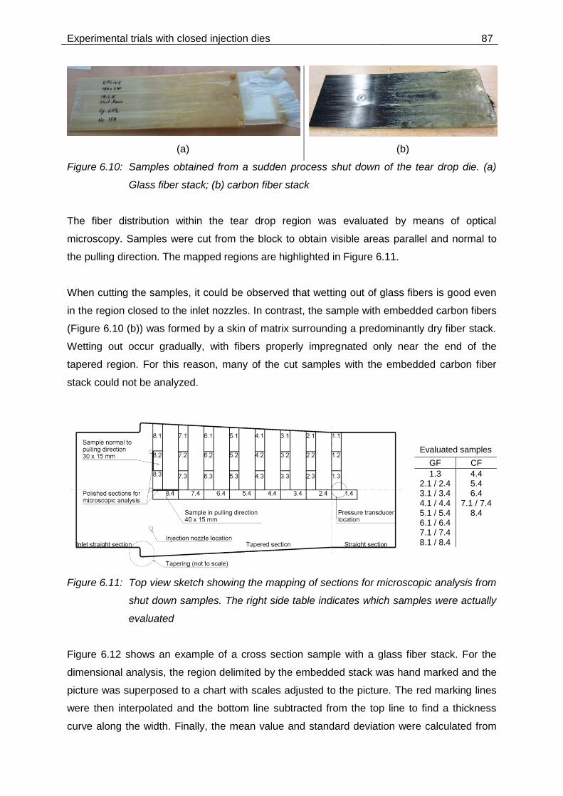
Experimental trials with closed injection dies 87
(a) (b)
Figure 6.10: Samples obtained from a sudden process shut down of the tear drop die. (a)
Glass fiber stack; (b) carbon fiber stack
The fiber distribution within the tear drop region was evaluated by means of optical
microscopy. Samples were cut from the block to obtain visible areas parallel and normal to
the pulling direction. The mapped regions are highlighted in Figure 6.11.
When cutting the samples, it could be observed that wetting out of glass fibers is good even
in the region closed to the inlet nozzles. In contrast, the sample with embedded carbon fibers
(Figure 6.10 (b)) was formed by a skin of matrix surrounding a predominantly dry fiber stack.
Wetting out occur gradually, with fibers properly impregnated only near the end of the
tapered region. For this reason, many of the cut samples with the embedded carbon fiber
stack could not be analyzed.
Evaluated samples
GF CF
1.3 2.1 / 2.4 3.1 / 3.4 4.1 / 4.4 5.1 / 5.4 6.1 / 6.4 7.1 / 7.4 8.1 / 8.4
4.4 5.4 6.4
7.1 / 7.4 8.4
Figure 6.11: Top view sketch showing the mapping of sections for microscopic analysis from
shut down samples. The right side table indicates which samples were actually
evaluated
Figure 6.12 shows an example of a cross section sample with a glass fiber stack. For the
dimensional analysis, the region delimited by the embedded stack was hand marked and the
picture was superposed to a chart with scales adjusted to the picture. The red marking lines
were then interpolated and the bottom line subtracted from the top line to find a thickness
curve along the width. Finally, the mean value and standard deviation were calculated from
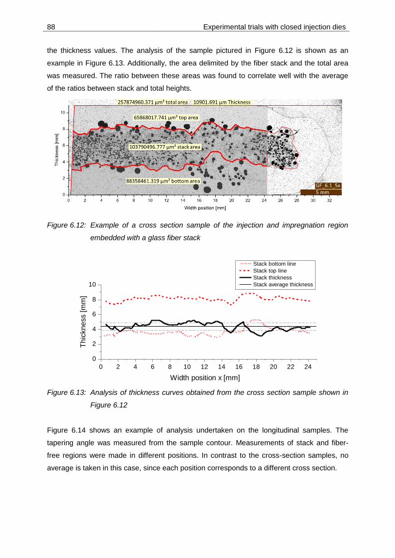
88 Experimental trials with closed injection dies
the thickness values. The analysis of the sample pictured in Figure 6.12 is shown as an
example in Figure 6.13. Additionally, the area delimited by the fiber stack and the total area
was measured. The ratio between these areas was found to correlate well with the average
of the ratios between stack and total heights.
Figure 6.12: Example of a cross section sample of the injection and impregnation region
embedded with a glass fiber stack
Figure 6.13: Analysis of thickness curves obtained from the cross section sample shown in
Figure 6.12
Figure 6.14 shows an example of analysis undertaken on the longitudinal samples. The
tapering angle was measured from the sample contour. Measurements of stack and fiber-
free regions were made in different positions. In contrast to the cross-section samples, no
average is taken in this case, since each position corresponds to a different cross section.
0 2 4 6 8 10 12 14 16 18 20 22 24
0
2
4
6
8
10
Th
ickn
ess [
mm
]
Width position x [mm]
Stack bottom line
Stack top line
Stack thickness
Stack average thickness

Experimental trials with closed injection dies 89
Figure 6.14: Example of a longitudinal sample of the injection and impregnation region
embedded with a glass fiber stack
The results for the microscopic analysis of the samples embedded with glass and carbon
fiber stacks are summarized in Figure 6.15. From observation of the different samples, it can
be stated that the fiber stack lies stretched with a nearly constant thickness over the free
volume region of the injection chamber. This was observed by the average values of cross
section samples embedded with the glass fiber stack, represented by the blue points, and by
most of the values taken from longitudinal samples (red points). The constant thickness
prevails up to the x-position where the die tapering has the same thickness as the fiber stack.
From this point on, the fiber stack was compressed along the tapered cavity similarly to the
conical die.
Figure 6.15: Results from microscopic dimensional analysis on longitudinal and cross
section samples embedded with a glass fiber stack
100 125 150 175 200 225 250 275 300 325 350 375 400 425
0
2
4
6
8
10
12
14
16
Thic
kness [m
m]
x-position from die inlet [mm]
Thickness of die cross section
Glass fiber stack
Injection section (longitudinal samples)
Embedded fibers (longitudinal samples)
Embedded fibers (cross section samples)
Profile assumed for the modeling
Carbon fiber stack
Embedded fibers (longitudinal samples)
Profile assumed for the modeling

90 Experimental trials with closed injection dies
The thicknesses measured for the injection region with the embedded glass fiber stack (black
points) agreed well with the nominal values according to the die design (black line), indicating
that no significant shape distortion occurred during the curing and/or sample preparation
process. On the other hand, samples with carbon fiber stacks showed very different
thicknesses because of the largely dry fiber stack surrounded by the cured matrix. For these
samples, a correction for the measured thickness of the fiber stack region was done, so that
the sum of thicknesses is equal to the nominal die thickness. The green points shown in
Figure 6.15 represent the corrected values of the embedded stack.
For modelling purposes, a constant thickness in the free volume injection region was
assumed. The thickness was calculated from all values obtained from cross section samples
(blue points) as (4.7 ± 0.8) mm. Although gradients in the fiber agglomeration within the stack
can be seen in the micrographs, for simplification the thickness was assumed as having a
constant fiber volume content of 34.1 %. For the carbon fiber stack, an average thickness of
(4.0 ± 0.2) mm was calculated, corresponding to a fiber volume content of 39.5 %. The blue
and green lines in Figure 6.15 represent the thickness profile assumed in the model
development (see Section 7.1.3.2).

Modelling and simulation of the closed injection pultrusion 91
7 Modelling and simulation of the closed injection pultrusion
The development of simulation models useful for the analysis of processing phenomena
within closed injection pultrusion dies is described in Section 7.1. Aspects of the geometric
design, meshing of the simulation domain and implementation in the preprocessor
environment are discussed. The material models developed in Sections 4 and 5 are also fed
to the simulation model as input parameters. The development of a simulation code used to
predict pressure variations in the straight die section due to thermal expansion and curing
effects is described, as well as the strategy for coupling the two different simulation models.
In section 7.2, results of several simulation runs used to predict different physical
phenomena are presented and discussed.
7.1 Modelling of the closed injection pultrusion
Based on the dies presented in Section 6, two models are developed in this section and
applied in the simulation studies (Section 7.2). The models include the geometrical design of
each die, which is spatially discretized into a mesh, its boundary conditions and other
constraints. A 2D geometry simplification was chosen for the conical die and a 3D model was
developed for the tear drop die.
The commercial software package used in the simulation studies, Ansys CFX 14.0, is built
upon a finite volume discretization method. In contrast to the finite element method, the
domain discretization in plane (2D) elements is not possible, i.e. the mesh elements and
domains are always volumetric. To overcome this limitation, one can build a quasi 2D model
as a very thin layer and set the side boundaries as a symmetry condition.
After designing the geometric model, the quasi 2D or 3D volume is spatially discretized by
dividing it into volume elements. The mesh in a quasi 2D model is set to have one element
thickness. Mesh resolution is a very important aspect in the spatial discretization process, in
which a balance must be found between obtaining fast enough simulations with the available
computational resources and realistic simulation results. This is typically done by comparing
simulation results obtained from meshes with different element sizes.
Another important aspect of the discretization process is mesh quality. In the Ansys CFX
best practice guidelines, some recommendations are given for grid generation. Whenever
feasible, a so-called structured mesh, i.e. a regular grid with ordered elements, e.g.
hexahedrons, should be implemented. Sharp angles in tetrahedral and pyramid elements

92 Modelling and simulation of the closed injection pultrusion
should be avoided. Highly skewed faces and elements are unacceptable because the
equations being solved assume that the cells are relatively equilateral/equiangular. The
meshing application included in the Ansys Workbench was used to generate all meshes in
this study. It provides several indexes of meshing quality. In this work, the skewness was
monitored to assess mesh quality. The skewness value determines how close to ideal, i.e.
equilateral or equiangular, a face or element is. It is therefore also correlated to the
orthogonal quality. Table 7.1 lists the values of skewness and the corresponding element
quality. Quality grids have an average skewness value of approximately 0.1 for 2D and 0.4
for 3D. In 3D grids of complex geometry, a small percentage will generally be in the fair
range and even a few poor cells may be accepted [81].
Table 7.1: Classification of element quality according to the skewness values
Value of Skewness
0 0 – 0.25 0.25 – 0.5 0.5 – 0.75 0.75 – 0.9 0.9 - 1 1
Element quality
Equilateral Excellent Good Fair Poor Bad Collapsed
The geometric design is subdivided into different volumetric regions, which are then assigned
to different domains. In the simulations conducted in these studies, three types of domains
are applied:
Solid domains, in which only the energy equations are solved, and may be typically
discretized to courser meshes
Liquid domains, where flow of liquid resin is calculated, together with the energy balance
Porous domains, where the flow of resin through a porous medium (the fiber stack) is
solved
There are two alternatives for calculating flow in porous media in CFX [81]. The first one is to
apply a fluid domain together with a model for momentum loss, which accounts for the
effects of porosity. This is named the superficial velocity formulation in CFX. The second
option is a full porous model, in which all governing equations are changed, and thus the
solid material properties and interactions between liquid and solid parts of the domain, e.g.
heat transfer, are calculated. The latter model was applied throughout this work.
Besides the assignment of domains, the model definition in the preprocessor includes the
setting of boundary conditions and material parameters. The boundary conditions are
specific for each die design and are discussed in Section 7.1.3. The material parameters
obtained from the models developed in Sections 4 and 5 are applied in the model definition.

Modelling and simulation of the closed injection pultrusion 93
The porous model supports the definition of two permeability parameters: one in the
streamwise and one in the transverse direction. The streamwise direction can be defined by
any vector direction in the Cartesian space. In this work, the streamwise direction, i.e. the
main direction of flow is defined as coincident with the x-axis. This is also the pulling
direction. Consequently, the permeability along the x-axis is set as 𝐾1 and along the y- and z-
axis are equal to 𝐾2 (see Section 5.3.2).
The curing reaction is implemented by means of an additional variable (the degree of cure 𝛼)
in Ansys CFX. It is treated by the solver as a non-reacting scalar component that is
transported through the fluid [81]. Two source terms in the liquid part of the porous domain
are associated with this additional variable: the source of 𝛼 itself, described by Equations 4.5
through 4.8, and an energy source given by Equation 4.9.
With the calculated local degree of cure, the local resin viscosity can be obtained from
Equation 3.16 and the parameters listed in Table 4.5. However, the software becomes
unstable when a high viscosity value is set, since its solving algorithm was developed for the
computation of turbulent flow of low viscosity liquids and gases. To overcome instability
issues during the calculations, the viscosity is defined as the minimum between the value
calculated by Equation 3.16 and 10 Pa·s.
7.1.1 Geometric design
The existing pultrusion dies were designed in the Ansys Workbench CAD tool
(DesignModeler) in a simplified form containing the geometric parameters relevant for the
subsequent simulation studies. The advantage of using the integrated CAD tool is the
possibility of easily defining design parameters which can be later parametrized and
automatically updated during sequential simulation runs. Two different approaches were
chosen for the different dies with the purpose of analyzing the reasonability of increased
model complexity in contrast to the results obtained. The design simplification included the
use of symmetry and the appropriate elimination of features such as small radii to reduce the
overall size and complexity of the mesh.
7.1.1.1 Conical die
For the conical die, a thin layer model was designed with the same geometric parameters as
the die used in the trials (see Section 6.1.1). The layer thickness was set to 0.3 mm. Only

94 Modelling and simulation of the closed injection pultrusion
half of the geometry was designed considering the die symmetry along the die centerline. A
symmetry condition was therefore set to the bottom surface of the model. The geometric
model is shown in Figure 7.1, in which the four existing domains are shown up to the
beginning of the straight curing section. The metal die region was set as a solid domain. The
injection nozzle was set as a fluid domain. The region through which the fibers are pulled
was set as a porous domain.
Figure 7.1: Geometric quasi 2D model of conical die (curing section not shown entirely)
The model was parametrized so that changes could be easily made in geometric design. To
study increasingly complex material models, two geometric designs were set. The first one
had a conical length L (see Figure 7.5) of 410 mm, i.e. the region upstream of the opening to
the atmosphere (see Figure 6.1) was excluded from the domain. The second one reproduced
the whole actual length of the inlet chamber. The set geometric parameters for the second
model of the complete die described above are listed in Table 7.2.
Table 7.2: Geometric parameters set in the conical die design
Geometric parameter Default value
Composite thickness [mm] 2,0
Length of the conical section [mm] 500
Angle of conical section [°] 1
Nozzle diameter [mm] 6
Inlet nozzle x-position [mm] 200
The surfaces at the top of the die where the cooling plate and electrical heaters were located
were also defined during the design phase. Values of heat fluxes were set to these surfaces
during the model setup (see Section 7.1.3).

Modelling and simulation of the closed injection pultrusion 95
7.1.1.2 Tear drop die
A 3D geometric model was developed for the tear drop die. From observations made during
the trials, the short resin pot life associated with the specific chamber design led to
stagnation regions of relatively long residence time, where resin locally gels (see
Section 6.2.2). As processing time progressed, the chamber became gradually filled with
gelled matrix. A fluid flow simulation within a 3D volumetric field is expected to deliver a
better representation of such stagnation regions, in comparison to a quasi 2D model like the
one developed for the conical die.
A 3D model representing ¼ of the die was designed as shown in Figure 7.2, according to die
symmetry. All main dimensions were designed as the actual die (see Section 6.1.2). The only
simplification made was the exclusion of edge radii existent at the entrance section, i.e. at
the die inlet and at the transition from the entrance to the tapered section, and at the outlet.
Similarly to the procedure adopted when designing the conical die, the cooling and heating
zones were assigned to surfaces delimited by the top surface of the solid domain.
Figure 7.2: 3D geometric model of tear drop die (curing section not shown entirely)
The geometric details of the die are also parametrized, as done in the conical die design.
This allows modifications of the geometry in order to perform parametric studies (see Section
7.2.3). Table 7.3 lists the set geometric parameters for the tear drop die described above.
In order to evaluate only curing aspects in steady state, another geometrical design was set
with a constant cross section over the whole die length, i.e. excluding the injection and
impregnation region. This is needed because the relatively large impregnation region volume
leads to ever growing reaction conversion at low local velocity spots. The steady state
computation is thus unstable in this configuration.
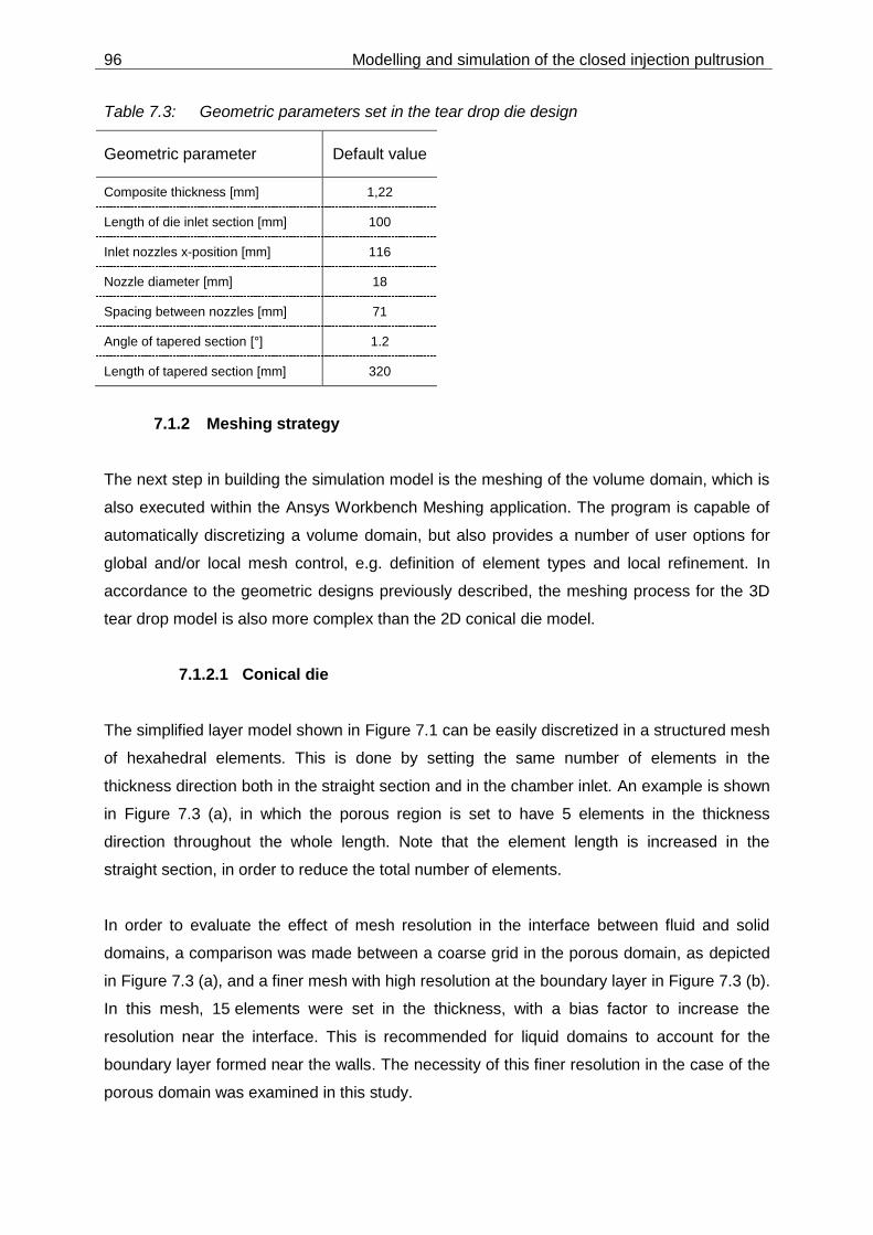
96 Modelling and simulation of the closed injection pultrusion
Table 7.3: Geometric parameters set in the tear drop die design
Geometric parameter Default value
Composite thickness [mm] 1,22
Length of die inlet section [mm] 100
Inlet nozzles x-position [mm] 116
Nozzle diameter [mm] 18
Spacing between nozzles [mm] 71
Angle of tapered section [°] 1.2
Length of tapered section [mm] 320
7.1.2 Meshing strategy
The next step in building the simulation model is the meshing of the volume domain, which is
also executed within the Ansys Workbench Meshing application. The program is capable of
automatically discretizing a volume domain, but also provides a number of user options for
global and/or local mesh control, e.g. definition of element types and local refinement. In
accordance to the geometric designs previously described, the meshing process for the 3D
tear drop model is also more complex than the 2D conical die model.
7.1.2.1 Conical die
The simplified layer model shown in Figure 7.1 can be easily discretized in a structured mesh
of hexahedral elements. This is done by setting the same number of elements in the
thickness direction both in the straight section and in the chamber inlet. An example is shown
in Figure 7.3 (a), in which the porous region is set to have 5 elements in the thickness
direction throughout the whole length. Note that the element length is increased in the
straight section, in order to reduce the total number of elements.
In order to evaluate the effect of mesh resolution in the interface between fluid and solid
domains, a comparison was made between a coarse grid in the porous domain, as depicted
in Figure 7.3 (a), and a finer mesh with high resolution at the boundary layer in Figure 7.3 (b).
In this mesh, 15 elements were set in the thickness, with a bias factor to increase the
resolution near the interface. This is recommended for liquid domains to account for the
boundary layer formed near the walls. The necessity of this finer resolution in the case of the
porous domain was examined in this study.

Modelling and simulation of the closed injection pultrusion 97
The generation of a high resolution mesh according to this strategy leads to very thin
elements, i.e. with a large length to thickness ratio, especially at the straight section near the
outlet of the porous region. This was however preferred over the generation of an
unstructured mesh with poor levels of orthogonality.
(a) (b)
Figure 7.3: (a) Example of local mesh for the conical die quasi 2D model; (b) zoomed view
of the mesh with high resolution at the solid-porous interface, in the transition
region conical-straight in the conical die model
7.1.2.2 Tear drop die
Due to the increased geometric complexity, finding a suitable and reliable meshing strategy
for the tear drop design is more challenging than in the case of the conical die. On the other
hand, further simplification of the design geometry is not desirable, as the primary interest is
to calculate the flow field within the more complex tapered section. Defining a reliable
meshing strategy is even more important when considering parametric studies, as the
geometry and subsequently the meshing process are ideally updated automatically, i.e.
without further manipulating the meshing setup configuration.
The most consistent meshing method found requires further subdivision of the whole porous
domain (green body in Figure 7.2) into several separate bodies in the design application: the
die inlet and the curing sections, which can be meshed to a similar structured grid composed
of hexahedral elements, and the injection and impregnation section (including the injection
nozzles), which is further subdivided into four sections. Figure 7.4 shows a top view of the
porous domain subdivided into meshing sections. The meshing process is conducted
sequentially for the six defined bodies in the shown order sequence. The section denoted as
1 is the die inlet section denoted in Figure 7.2, and section 2 is the beginning of the curing
region. The die body is meshed in a last step (denominated as 7). By the sequential meshing
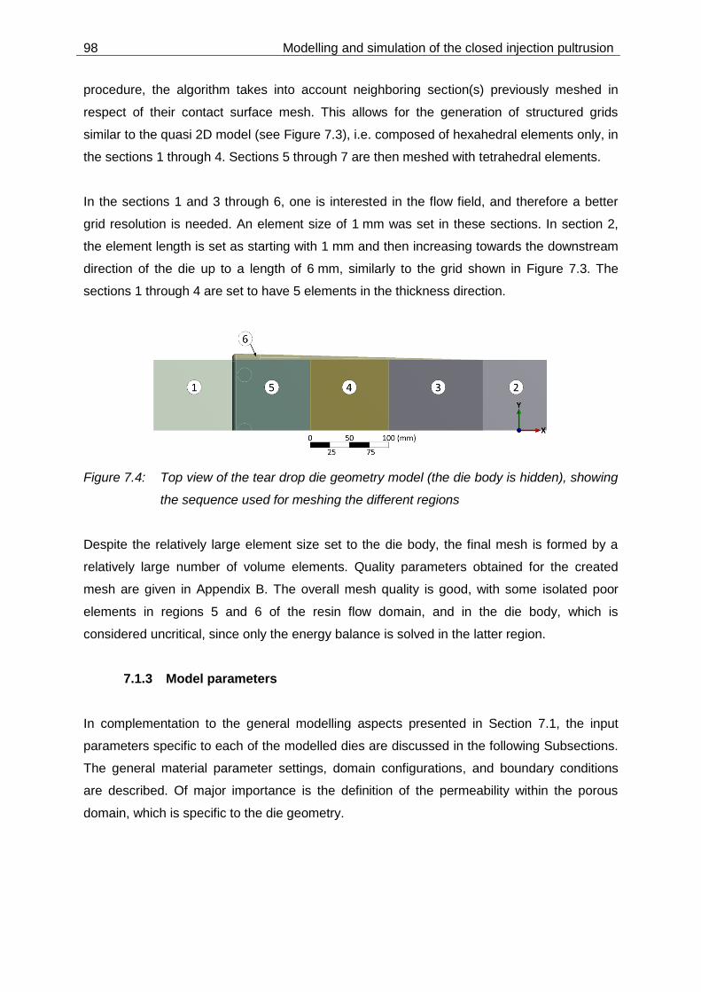
98 Modelling and simulation of the closed injection pultrusion
procedure, the algorithm takes into account neighboring section(s) previously meshed in
respect of their contact surface mesh. This allows for the generation of structured grids
similar to the quasi 2D model (see Figure 7.3), i.e. composed of hexahedral elements only, in
the sections 1 through 4. Sections 5 through 7 are then meshed with tetrahedral elements.
In the sections 1 and 3 through 6, one is interested in the flow field, and therefore a better
grid resolution is needed. An element size of 1 mm was set in these sections. In section 2,
the element length is set as starting with 1 mm and then increasing towards the downstream
direction of the die up to a length of 6 mm, similarly to the grid shown in Figure 7.3. The
sections 1 through 4 are set to have 5 elements in the thickness direction.
Figure 7.4: Top view of the tear drop die geometry model (the die body is hidden), showing
the sequence used for meshing the different regions
Despite the relatively large element size set to the die body, the final mesh is formed by a
relatively large number of volume elements. Quality parameters obtained for the created
mesh are given in Appendix B. The overall mesh quality is good, with some isolated poor
elements in regions 5 and 6 of the resin flow domain, and in the die body, which is
considered uncritical, since only the energy balance is solved in the latter region.
7.1.3 Model parameters
In complementation to the general modelling aspects presented in Section 7.1, the input
parameters specific to each of the modelled dies are discussed in the following Subsections.
The general material parameter settings, domain configurations, and boundary conditions
are described. Of major importance is the definition of the permeability within the porous
domain, which is specific to the die geometry.

Modelling and simulation of the closed injection pultrusion 99
7.1.3.1 Conical die
In the straight section of the conical die, the fiber volume content is constant. In the tapered
section, the porosity and consequently the permeabilities vary according to the position along
the x-axis. Two models of increasing complexity are proposed and applied in this study. The
first simplified model assumes that the fibers are distributed uniformly across the thickness
direction within the tapered region. For a unidirectional roving stack, the porosity is calculated
from Equation 7.1 and the corresponding geometric parameters shown in Figure 7.5. The
fiber volume fraction along the conical section, 𝑉𝑓𝑥, is given by Equation 7.2 as a function of
the geometric parameters and the final volume fraction 𝑉𝑓 in the straight section.
𝜙𝑥 = 1 −
ℎ𝑐(1 − 𝜙𝑐)
ℎ𝑐 + (𝐿 − 𝑥) 𝑡𝑎𝑛 𝜃 Equation 7.1
𝑉𝑓𝑥 = 1 − 𝜙𝑥 =
ℎ𝑐 ∙ 𝑉𝑓
ℎ𝑐 + (𝐿 − 𝑥) 𝑡𝑎𝑛 𝜃 Equation 7.2
Figure 7.5: Geometric parameters of the tapered inlet used for calculating the local porosity
of the fiber stack as a function of the x position
The second model proposed considers the inhomogeneous distribution of fiber bundles
within the tapered region. In the conical die assembly, the fiber bundles are threaded through
a guiding plate with a specific hole pattern. These bundles are therefore actually separated
from each other during the pulling process until they reach a point in the tapered region
where the stack is compacted. Figure 7.6 schematically depicts the fiber bundle distribution
within the tapered region and how it is converted to a simplified porosity distribution in the
simulation model.

100 Modelling and simulation of the closed injection pultrusion
(a) (b)
Figure 7.6: (a) Schematic representation of fiber bundle distribution within the tapered
region, according to experimental assembly; (b) Porosity distribution applied to
porous domain in the simulation model
Within the inhomogeneous region, the fiber bundles have a constant porosity 𝜙0 = 0.65,
which is the value of porosity at zero compaction pressure found in compressibility
measurements (see Table 5.4). For simplification purposes, the respective regions of fiber
bundles and neat resin are assembled together and assigned to the regions depicted in
Figure 7.6 (b). A very large porosity of 0.99 is assigned to the neat resin region. The function
𝜙𝑥 is calculated according to Equation 7.1.
Figure 7.7 shows the values of porosity and the permeability values K1 and K2 for a fiber
volume fraction of 64 % in the straight section of the die. The permeabilities are calculated
according to the Gebart functions (Equation 3.19 and Equation 3.20) and the equivalent fiber
diameters obtained from the fitting procedure discussed in Section 5.3.2. For the second
model, the position along the tapered section from which the fiber stack is compacted is
found as x = 405 mm, where the porosity is equal to 0.65.
Figure 7.7: Porosity and permeability coefficients of a roving stack as a function of the x
position in the tapered section of the conical die.
0 100 200 300 400 500
0.0
0.2
0.4
0.6
0.8
1.0
Poro
sity
Position x [mm]
Porosity
K1
K2
Porosity threshold 0.65
10-14
10-13
10-12
10-11
10-10
10-9
10-8
10-7
10-6
10-5
K1, K
2 [m
²]

Modelling and simulation of the closed injection pultrusion 101
The permeability function of a CFM / roving / CFM reinforcement stack along the tapered
section cannot be directly calculated as the above unidirectional case. The individual
thicknesses of each layer as function of mechanical pressure must be taken into account.
The following procedure is used to calculate the permeabilities:
1. Define a compaction pressure for the stack in the final profile cross section (90 x 2 mm²).
The pressure was set to 2.1 bar in this study
2. Calculate the thickness of the roving layer by subtracting the thickness of CFM layer
(0.49 mm in this study) for the given compaction pressure
3. Calculate the number of rovings needed to fill the remaining 90 x 1.51 mm² cross section
(83 rovings in this study)
4. Obtain curves of thickness vs compaction pressure in the range 0 – 2.1 bar. The
maximum thickness (zero compaction pressure) found for the stack is 3.61 mm. The
CFM layer thickness (1.14 mm) is considered constant and only the roving layer fills the
tapered region where the cavity height (ℎ𝑐 + ℎ𝑥′) is larger than 7.23 mm
5. Calculate the porosity and permeability distributions along the x-axis for each layer
Figure 7.8 shows the values of porosity and the longitudinal permeability 𝐾1 calculated
according to the procedure described above. The roving layer permeability is calculated
according to the Gebart function and the CFM permeability according to the Kozeny-Carman
model with the adjusted longitudinal constant shown in Figure 5.13. The implementation of
individual layers in the CFX preprocessor considers the conventional stacking sequence of
pultruded laminates with the CFM as an outer layer. In the model, this results in a region with
constant thickness running parallel to the tapered wall up to approximately 400 mm from the
die inlet. From this point on, it is compressed together with the roving layer until the end
thickness is reached. Due to the increased complexity of this multilayered case, the
inhomogeneity in the roving layer is not implemented in this model, as previously done for
the unidirectional case.
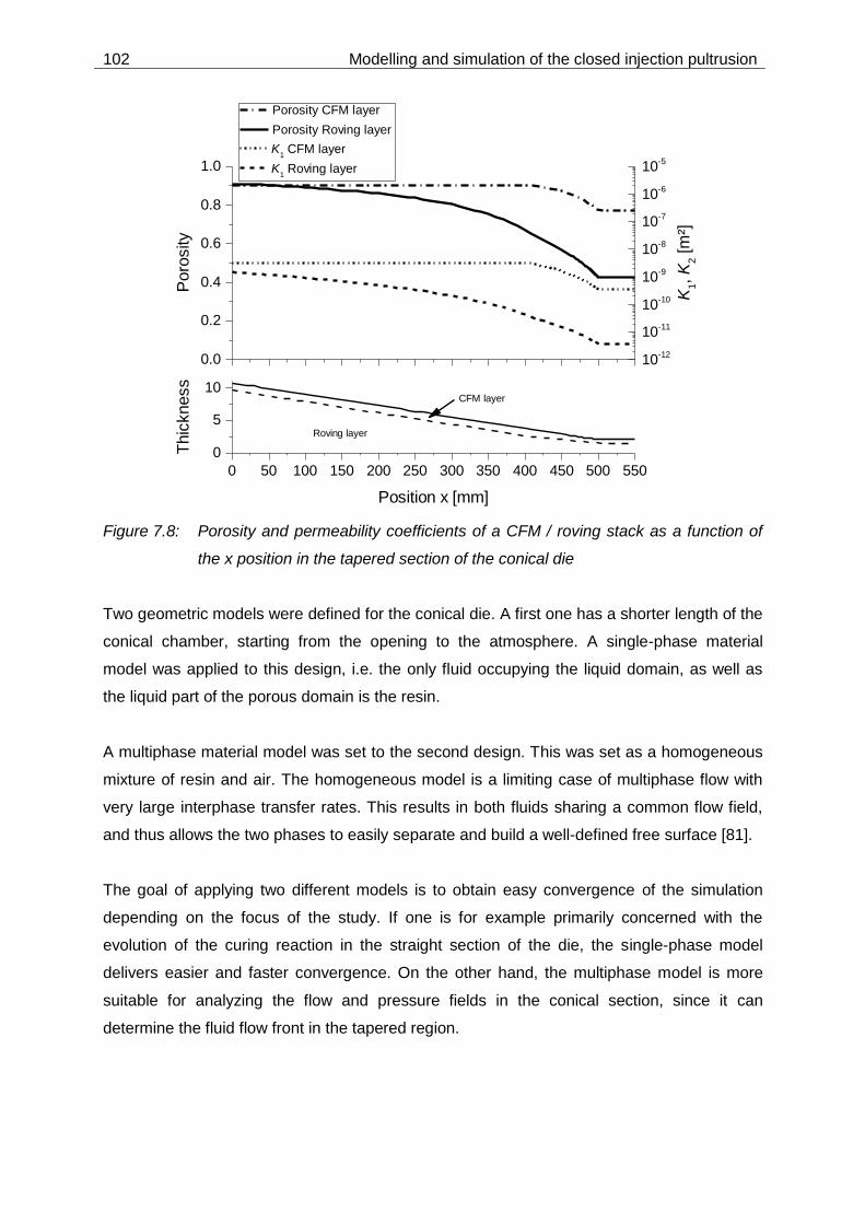
102 Modelling and simulation of the closed injection pultrusion
Figure 7.8: Porosity and permeability coefficients of a CFM / roving stack as a function of
the x position in the tapered section of the conical die
Two geometric models were defined for the conical die. A first one has a shorter length of the
conical chamber, starting from the opening to the atmosphere. A single-phase material
model was applied to this design, i.e. the only fluid occupying the liquid domain, as well as
the liquid part of the porous domain is the resin.
A multiphase material model was set to the second design. This was set as a homogeneous
mixture of resin and air. The homogeneous model is a limiting case of multiphase flow with
very large interphase transfer rates. This results in both fluids sharing a common flow field,
and thus allows the two phases to easily separate and build a well-defined free surface [81].
The goal of applying two different models is to obtain easy convergence of the simulation
depending on the focus of the study. If one is for example primarily concerned with the
evolution of the curing reaction in the straight section of the die, the single-phase model
delivers easier and faster convergence. On the other hand, the multiphase model is more
suitable for analyzing the flow and pressure fields in the conical section, since it can
determine the fluid flow front in the tapered region.
0 50 100 150 200 250 300 350 400 450 500 550
0
5
10
Thic
kness
Position x [mm]
CFM layer
Roving layer
0.0
0.2
0.4
0.6
0.8
1.0
Porosity CFM layer
Porosity Roving layer
Poro
sity
10-12
10-11
10-10
10-9
10-8
10-7
10-6
10-5
K1 CFM layer
K1 Roving layer
K1, K
2 [m
²]

Modelling and simulation of the closed injection pultrusion 103
There are two inlet boundaries in the model: the resin inlet is set at a constant pressure, and
the fibers inlet is set as an entrainment, i.e. an opening in which flow inwards and/or
outwards is allowed. The outlet is set at a normal speed condition equal to the pulling speed.
Heat transfer between the solid domain and the environment is done by different surfaces
assigned as one of the following options with corresponding boundary conditions:
Wall: heat transfer coefficient (HTC): 10 W/(m² K)
Ambient temperature 25 °C, or actual temperature during the corresponding experimental
trial
Cooling zone: defined heat flux out of the domain
Heating zone: heat flux in or out of the domain, depending on the location
The heat transfer between porous and solid domains is determined by a thermal contact
resistance coefficient (TCR). According to Baran et al. [108], adjusting of this parameter is
necessary for pultrusion process simulations including the heat transfer between the
composite material and the solid die. An optimization procedure is presented in this study in
which local TCR values are found that lead to good fitting of simulation results to
experimental data. The reasoning for this is explained in the context of different material
states along the die.
7.1.3.2 Tear drop die
A single-phase material model was considered for the tear drop 3D design, since the flow
front is irrelevant in terms of process control, in contrast to the conical die. The cavity is
always full of resin at all times, and this condition is monitored by adjusting the flow rate such
that a small excess of resin flows out of the die inlet. The boundary conditions are defined
similarly to the conical die specifications described in the previous section.
The porosity and permeability distribution in the inlet region of the tear drop die is set
according to the analysis presented in Section 6.2.3. In the large volume inlet region, the
fiber stack is assumed to have a constant thickness. Furthermore, the fiber distribution within
this thickness is assumed to be uniform, and therefore constant porosity and permeability
parameters are attributed to the stack. Towards the end of the tapered section, the stack is
then constrained by the decreasing cross section area; the porosity and permeabilities
assume in this region a profile like the calculated for the conical die (see Figure 7.7). Figure
7.9 shows the curves implemented in the model, as a function of the position along the x-axis
from the die inlet.
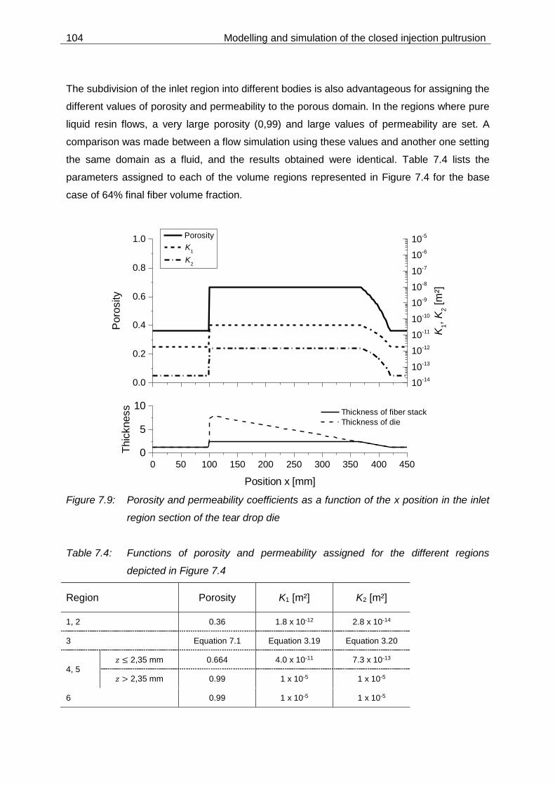
104 Modelling and simulation of the closed injection pultrusion
The subdivision of the inlet region into different bodies is also advantageous for assigning the
different values of porosity and permeability to the porous domain. In the regions where pure
liquid resin flows, a very large porosity (0,99) and large values of permeability are set. A
comparison was made between a flow simulation using these values and another one setting
the same domain as a fluid, and the results obtained were identical. Table 7.4 lists the
parameters assigned to each of the volume regions represented in Figure 7.4 for the base
case of 64% final fiber volume fraction.
Figure 7.9: Porosity and permeability coefficients as a function of the x position in the inlet
region section of the tear drop die
Table 7.4: Functions of porosity and permeability assigned for the different regions
depicted in Figure 7.4
Region Porosity K1 [m²] K2 [m²]
1, 2 0.36 1.8 x 10⁻¹² 2.8 x 10⁻¹⁴
3 Equation 7.1 Equation 3.19 Equation 3.20
4, 5 𝑧 ≤ 2,35 mm 0.664 4.0 x 10⁻¹¹ 7.3 x 10⁻¹³
𝑧 > 2,35 mm 0.99 1 x 10⁻⁵ 1 x 10⁻⁵
6 0.99 1 x 10⁻⁵ 1 x 10⁻⁵
0 50 100 150 200 250 300 350 400 450
0
5
10 Thickness of fiber stack
Thickness of die
Thic
kness
Position x [mm]
0.0
0.2
0.4
0.6
0.8
1.0 Porosity
Poro
sity
10-14
10-13
10-12
10-11
10-10
10-9
10-8
10-7
10-6
10-5
K1
K2
K1, K
2 [m
²]

Modelling and simulation of the closed injection pultrusion 105
In the curing simulations using the tear drop model, an unsteady state prevails due to the
large volume in the inlet region occupied by resin only. This leads to a continuously
increasing local degree of cure and reaction heat development. To overcome this, another
simplified model was implemented with the same die body outer dimensions but without the
injection and impregnation chamber.
7.1.4 Stress-strain model
A simulation code was written in the Wolfram language (Mathematica 9) based on the finite
difference (FD) iterative algorithm proposed by Bogetti and Gillespie [88] [89], and recently
applied by Baran et al [87] in pultrusion related studies. In these studies, the goal was to
obtain the development of internal stresses and distortions within the laminate as the matrix
cures. In the present study, this additional numerical solver is used for two purposes: (1) to
correct the temperature of the rheology measurements and obtain a more accurate
prediction for the degree of cure (see Section 4.4) and (2) to obtain a more realistic pressure
distribution within the straight curing section of the die. The pressure changes within the
region are modelled as being caused by two concurrent effects: the thermal expansion due
to temperature increase within the material and volume shrinkage of the matrix as curing
progresses. These effects on the resulting pressure in the die cavity cannot be calculated by
CFX, since the coefficient of thermal expansion (CTE) is only used there to account for
buoyancy effects in gases.
7.1.4.1 Model development and validation
The code was implemented as an alternating difference explicit (ADE) discretization method
over a 2D domain representing the die cavity cross section. For the conical model, the 2D
model reduces to a quasi 1D model with a very thin width and the minimum of 3 nodes in the
y-direction, to allow for solving of the discretization equations in the same way as in a full 2D
model. The spatial discretization is shown in Figure 7.10. By the ADE method, two sweeps,
forward and backward are done in each iteration. The calculation of the temperature at a
node i, j is done by each sweep from the known values at four adjacent nodes. The
temperature at node i, j for that iteration step is then taken as the average value from both
sweep results. The model is a time marching procedure, i.e. each iteration step corresponds
to a real increment in time by the time step ∆𝑡.

106 Modelling and simulation of the closed injection pultrusion
Figure 7.10: Grid definition showing nodes used to calculate the temperature and degree of
cure fields and stress-strain relationships
The model was validated by running the same simulations for a plane stress assumption
reported in [87] - [89]. The results obtained were similar to the literature reports. A
comparison for some of the simulations is shown in Figure 7.11. For the pultrusion case, a
plane strain assumption is applied for the profile cross section (see next section).
(a) (b)
Figure 7.11: Comparison of results obtained from developed simulation code and results
available in the literature [87] [89]. Predicted in-plane transverse stress for (a)
different composite thicknesses and (b) different resin shrinkage factors
The kinetic model developed in Section 4.3 was applied to the implemented code for the
calculation of degree of cure and temperature in a 2D field. The temperature function of time
according to the heating rate was set as a prescribed value (Dirichlet condition). The curves
-100 -75 -50 -25 0 25 50 75 1000.0
0.1
0.2
0.3
0.4
0.5
Bogetti and Gillespie [89]
Baran et al. [87]
2D model developed in this work
Dim
en
sio
nle
ss th
ickn
ess
Transverse stress [MPa]
25.4 mm25.4 mm
50.8 mm
76.2 mm
-10 -5 0 5 10 15 200.0
0.1
0.2
0.3
0.4
0.5
0%1%3%
Bogetti and Gillespie [89]
Baran et al. [87]
2D model developed in this work
Dim
en
sio
nle
ss th
ickn
ess
Transverse stress [MPa]
6%

Modelling and simulation of the closed injection pultrusion 107
obtained by the NETZSCH Thermokinetics software and the implemented algorithm for the
heating rates measured in DSC are compared in Figure 7.12.
Figure 7.12: Degree of cure development as calculated by the Kinetics software and the
Finite Difference (FD) model for different heating rates
Very similar plots are obtained by both calculations, thus giving confidence on the validity of
the implemented algorithm. The use of this code has the advantage of taking into account
the effects of heat conduction and of internal heat generation within the material on the
temperature, and thus on acceleration of the reaction rate. An example of these effects is
shown in Figure 7.13. The curves of degree of cure and temperature development for a
heating rate of 5 K/min are plotted as calculated by the Kinetics software, as well as for 2D
fields with 25 x 1 mm² and 25 x 2 mm² calculated by the implemented code. Plots are given
for a point in the center of the 2D field, designated as bulk. It can be seen that the first
reaction step evolves relatively smoothly, so that no significant temperature peak due to
exothermic heat release is observed. The second reaction, on the other hand, evolves very
fast, leading to a pronounced local temperature increase and faster curing in the bulk of the
material. The extent of temperature increase and reaction acceleration is sensitive to the
material thickness. A less pronounced temperature increase can also be detected at the
margin of the 2D field, corresponding to the material surface (not shown in the plot).
-20 0 20 40 60 80 100 120 140 160 1800.0
0.2
0.4
0.6
0.8
1.0D
egre
e o
f C
ure
Temperature [°C]
5 K/min Kinetics
1 K/min Kinetics
0.5 K/min Kinetics
5 K/min FD-Model timestep 0.1s
1 K/min FD-Model timestep 0.1s
0.5 K/min FD-Model timestep 0.1s

108 Modelling and simulation of the closed injection pultrusion
Figure 7.13: Degree of cure development and temperature for 2D fields of 1 and 2 mm
thicknesses
7.1.4.2 Application in pultrusion process
Considering the coordinate system universally used in classical laminate theory, i.e. 1 being
the main fiber orientation direction, 2 the cross direction and 3 the out-of-plane direction and
setting these directions coincident with the global Cartesian coordinates 𝑥𝑦𝑧, a transfer of the
model to the pultrusion process is depicted by Figure 7.14. As the material travels through
the die, the temperature and degree of cure development is iteratively calculated, and from
these values the stress-strain field is also obtained. In contrast to the results reported in [88]
and [89], the material properties are the same for both directions in the 2D field considered in
the pultrusion case. The time marching procedure translates to a Lagrangian framework in
which each time step corresponds to a forward step in the 𝑥 direction by 𝑈 ∙ ∆𝑡.
The simulation run calculates the temperature and degree of cure distributions within the
profile along the die, as well as the stress and strain in the cross section plane. A plane strain
assumption is applied to the cross section plane. Normal stresses acting at the domain
boundaries, i.e. at the material surface in contact to the die are calculated. These stresses
are calculated considering the fictive unconstrained strain distribution within the material, i.e.
as if the laminate was free to expand or shrink. However, the material is actually constrained
by the die inner walls, which are here assumed as perfectly rigid; therefore a normal stress of
the same magnitude but opposite direction is needed to “force” the material back to the
0 5 10 15 20 25 30 35 40
0.0
0.2
0.4
0.6
0.8
1.0
kinetics software
bulk, 1 mm thickness
bulk, 2 mm thickness
T bulk, 1 mm thickness
T bulk, 2 mm thicknessD
egre
e o
f cure
Time [min]
0
25
50
75
100
125
150
175
200
Tem
pera
ture
[°C
]
29 30 31 32 33
0.3
0.4
0.5
0.6
0.7
0.8
0.9
0
50
100
150
200
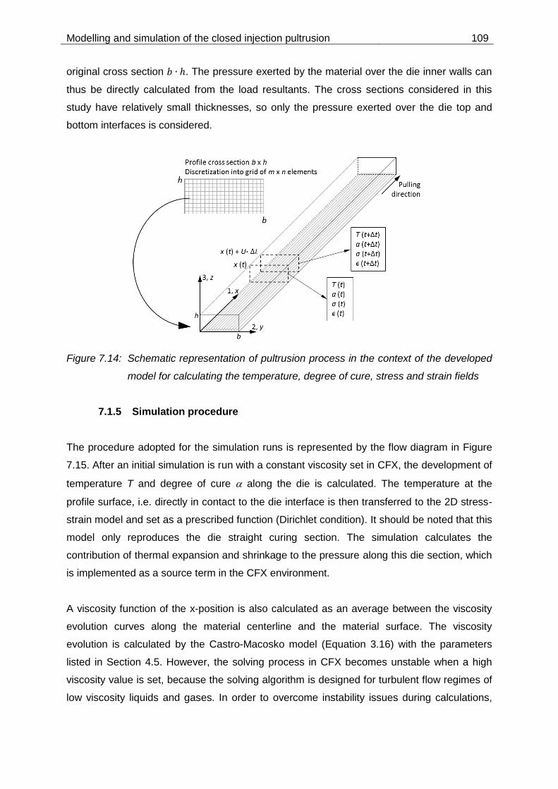
Modelling and simulation of the closed injection pultrusion 109
original cross section 𝑏 ∙ ℎ. The pressure exerted by the material over the die inner walls can
thus be directly calculated from the load resultants. The cross sections considered in this
study have relatively small thicknesses, so only the pressure exerted over the die top and
bottom interfaces is considered.
Figure 7.14: Schematic representation of pultrusion process in the context of the developed
model for calculating the temperature, degree of cure, stress and strain fields
7.1.5 Simulation procedure
The procedure adopted for the simulation runs is represented by the flow diagram in Figure
7.15. After an initial simulation is run with a constant viscosity set in CFX, the development of
temperature T and degree of cure along the die is calculated. The temperature at the
profile surface, i.e. directly in contact to the die interface is then transferred to the 2D stress-
strain model and set as a prescribed function (Dirichlet condition). It should be noted that this
model only reproduces the die straight curing section. The simulation calculates the
contribution of thermal expansion and shrinkage to the pressure along this die section, which
is implemented as a source term in the CFX environment.
A viscosity function of the x-position is also calculated as an average between the viscosity
evolution curves along the material centerline and the material surface. The viscosity
evolution is calculated by the Castro-Macosko model (Equation 3.16) with the parameters
listed in Section 4.5. However, the solving process in CFX becomes unstable when a high
viscosity value is set, because the solving algorithm is designed for turbulent flow regimes of
low viscosity liquids and gases. In order to overcome instability issues during calculations,
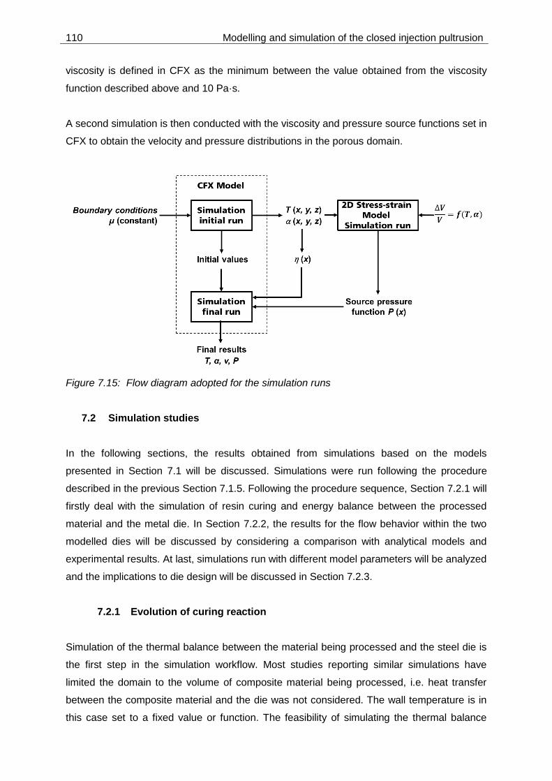
110 Modelling and simulation of the closed injection pultrusion
viscosity is defined in CFX as the minimum between the value obtained from the viscosity
function described above and 10 Pa·s.
A second simulation is then conducted with the viscosity and pressure source functions set in
CFX to obtain the velocity and pressure distributions in the porous domain.
Figure 7.15: Flow diagram adopted for the simulation runs
7.2 Simulation studies
In the following sections, the results obtained from simulations based on the models
presented in Section 7.1 will be discussed. Simulations were run following the procedure
described in the previous Section 7.1.5. Following the procedure sequence, Section 7.2.1 will
firstly deal with the simulation of resin curing and energy balance between the processed
material and the metal die. In Section 7.2.2, the results for the flow behavior within the two
modelled dies will be discussed by considering a comparison with analytical models and
experimental results. At last, simulations run with different model parameters will be analyzed
and the implications to die design will be discussed in Section 7.2.3.
7.2.1 Evolution of curing reaction
Simulation of the thermal balance between the material being processed and the steel die is
the first step in the simulation workflow. Most studies reporting similar simulations have
limited the domain to the volume of composite material being processed, i.e. heat transfer
between the composite material and the die was not considered. The wall temperature is in
this case set to a fixed value or function. The feasibility of simulating the thermal balance

Modelling and simulation of the closed injection pultrusion 111
between the composite material, including the curing resin and the metal die was
investigated in this study. The 2D conical die model and the 3D tear drop die model were
employed.
For the 2D conical die model, experimental temperature data from trial configuration 1 (refer
to Table 6.1, glass fiber volume content 64%, pulling speed 0.3 m/min, set temperature of
heating zones 100 °C), shown in Figure 6.3, was used to validate the simulation. Fixed heat
fluxes were set to the cooling and each of the heating zones. To find appropriate values of
heat fluxes, a first simulation was run with fixed temperatures at the cooling zone (20 °C) and
at heating zones (100 °C). The heat fluxes found by this simulation run are then used as an
initial guess for an optimization procedure to minimize the differences between the
temperature values measured by TCs, both located in the die and in the processed material,
and simulation results. The same method described in Section 5.1.3.2 to minimize pressure
residuals is applied in the optimization procedure.
Figure 7.16 shows the results of various simulations carried out with different set parameters.
The target temperatures used for the optimization procedure are shown as blue (TCs located
in the die body) and red (temperatures at the profile surface measured by wire TC) points.
The temperature prediction within the composite material along the die agrees reasonably
well with measured values. A better correlation is achieved by setting a Thermal Contact
Resistance coefficient (TCR) at the interface between the composite and die. The profile
surface temperature predictions from three simulation cases with different TCR values are
plotted: (1) 0 m².K/W over the whole die length, (2) 0.005 m².K/W over the die length and (3)
a variable TCR at different sections of the die (each section is 200 mm long), according to
the values plotted in the right axis. It can be concluded that a variable TCR along the die
length leads to a better correlation between temperatures as measured during processing
and obtained from simulations. Such a qualitative correlation was also observed in [108]. In
that study, a larger TCR in the region close to the die inlet was attributed to cooling channels
which were not explicitly modelled. One possible explanation for the larger TCR in the inlet
section found in the present study is a difference in material composition. The larger resin to
fiber ratio, leads to a proportionally lower thermal conductivity at the tapered section. This
effect is accentuated by the inhomogeneous distribution of the rovings, i.e. a resin-only film
actually exists at the contact interface, in contrast with the simplified, homogeneous porous
model.

112 Modelling and simulation of the closed injection pultrusion
Figure 7.16: Temperature curves obtained from simulations of the conical die model with
different set parameters
Figure 7.17 (top) shows a comparison of measured temperatures and the final simulation
results of the conical die. The bars located close to the x-axis reflect the positions of the die
cooling and heating zones. Good agreement is found between the measured temperature
evolution and the simulation results. Some discrepancy is observed near the exothermic
peak, where the predicted temperature increase is steeper than the experimental results.
Towards the downstream section there is another slight temperature increase in the fourth
heating zone, which is also not accurately reproduced by the simulation. In this section, TC
measurements in the die body show a lower value than predicted by simulation. However,
the temperature prediction within the processed material is close to the experimental data,
allowing for a realistic prediction of the degree of cure at the end of the die.
Figure 7.17 (bottom) shows the calculated degree of cure and viscosity evolution for the
conical die. A considerable portion of the reaction already takes place in the conical region,
as can be seen by both the increasing temperatures, as well as in the predicted degree of
cure. By the end of the conical section (x = 500 mm) approximately 5% conversion, i.e. about
17% of the B-staging reaction, is reached. However, viscosity remains low (under 1 Pa·s)
within the length of the conical region, which is a decisive factor for stable processing. It can
be seen that a viscosity drop occurs upon reaching the first heating zone, where the
temperature increase (Arrhenius relation) effect in the viscosity exceeds the reciprocal
network formation effect. This is immediately followed by a steep viscosity increase indicating
gelation at a distance of approximately 850 mm from the die inlet. Furthermore, a stable
0 200 400 600 800 1000 1200 1400 1600
20
40
60
80
100
120
Te
mp
era
ture
[°C
]
x-position from die inlet [mm]
Measured temperatures Temperatures predicted by simulation Optimum TCR values
Profile surface TC Fixed T at heating zones
Die T Fixed heat fluxes, TCR = 0 m².K/W
Profile surface T Fixed heat fluxes, TCR = 0.005 m².K/W
Fixed heat fluxes, optimized TCR
Optimum heat fluxes [W/m²]
Cooling zone = -9800
Heating zone 1 = 6305
Heating zone 2 = -1975
Heating zone 3 = -1103
Heating zone 4 = 2000
0.000
0.005
0.010
0.015
0.020
0.025
0.030
TC
R [
m².
K/W
]

Modelling and simulation of the closed injection pultrusion 113
processing to a B-stage product is reached, since the degree of cure approaches a plateau
at approximately 28% conversion, yet not triggering the second reaction step.
Figure 7.17: Top: comparison of experimental temperature data and simulation results along
the length of the conical die for trial configuration 1 (refer to Table 6.1); bottom:
predicted degree of cure and calculated viscosity along the die length
Comparison of the heat fluxes obtained from experimental data and simulation reveals that
the thermal balance in the metal die is not realistically reproduced, at least by the 2D
simulation. The heat flux from heating plates in zones 2 and 3 is close to zero (marginally
positive), while simulation results point out to a net heat flux out of the domain in these
regions. The pultrusion die has a larger surface area in contact to the ambient air (top area
between heating plates and side faces) than the 2D design. The heat dissipation is therefore
more constrained in the simulation model. Consequently, heating zones 2 and 3 act as a
heat sink to achieve a satisfactory energy balance within the composite material, i.e. to
obtain temperature prediction curves similar to measured data. The 3D simulation is
expected to deliver better results for the thermal balance, since the dimensions and
0 200 400 600 800 1000 1200 1400 1600
0.00
0.05
0.10
0.15
0.20
0.25
0.30 profile surface
profile center
Deg
ree
of
cu
re
x-position from die inlet [mm]
20
30
40
50
60
70
80
90
100
110
120 Profile surface TC
Profile center TC
Die control TC
Die monitoring TC
Profile surface simulation
Profile center simulation
Die temperature simulation
Te
mp
era
ture
[°C
]
102
103
104
105
Viscosity
Vis
co
sity [
mP
a.s
]
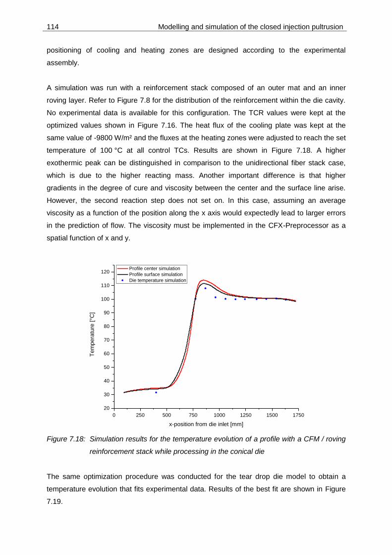
114 Modelling and simulation of the closed injection pultrusion
positioning of cooling and heating zones are designed according to the experimental
assembly.
A simulation was run with a reinforcement stack composed of an outer mat and an inner
roving layer. Refer to Figure 7.8 for the distribution of the reinforcement within the die cavity.
No experimental data is available for this configuration. The TCR values were kept at the
optimized values shown in Figure 7.16. The heat flux of the cooling plate was kept at the
same value of -9800 W/m² and the fluxes at the heating zones were adjusted to reach the set
temperature of 100 °C at all control TCs. Results are shown in Figure 7.18. A higher
exothermic peak can be distinguished in comparison to the unidirectional fiber stack case,
which is due to the higher reacting mass. Another important difference is that higher
gradients in the degree of cure and viscosity between the center and the surface line arise.
However, the second reaction step does not set on. In this case, assuming an average
viscosity as a function of the position along the x axis would expectedly lead to larger errors
in the prediction of flow. The viscosity must be implemented in the CFX-Preprocessor as a
spatial function of x and y.
Figure 7.18: Simulation results for the temperature evolution of a profile with a CFM / roving
reinforcement stack while processing in the conical die
The same optimization procedure was conducted for the tear drop die model to obtain a
temperature evolution that fits experimental data. Results of the best fit are shown in Figure
7.19.
0 250 500 750 1000 1250 1500 1750
20
30
40
50
60
70
80
90
100
110
120
Tem
pera
ture
[°C
]
x-position from die inlet [mm]
Profile center simulation
Profile surface simulation
Die temperature simulation

Modelling and simulation of the closed injection pultrusion 115
Figure 7.19: Top: comparison of experimental temperature data and simulation results along
the length of the tear drop die for trial configuration 9 (refer to Table 6.1);
bottom: predicted degree of cure and calculated viscosity along the die length
In this case, a better correlation is reached between the power inputs of the heating plates as
logged during experiments (see Figure 6.8) and predicted by the simulation, at least in
qualitative terms. A quantitative validation is not feasible at this stage; for such a comparison,
experimental electrical output data (apparent and effective power) would need to be
measured separately for each heating zone during a processing trial.
7.2.2 Flow behavior of liquid resin
Successful processing of a profile by means of closed injection pultrusion is determined by
the flow of liquid resin relatively to the moving reinforcement stack. In this case, the
compacted stack must be thoroughly wetted within a short impregnation chamber length
containing a relatively small resin volume. Understanding the aspects of resin flow are
therefore of vital importance in designing an appropriate injection and impregnation chamber
for a particular die. It is also evident that such a design will be intrinsically dependent on the
0 200 400 600 800 1000 1200
0.00
0.05
0.10
0.15
0.20
0.25
0.30 profile surface
profile center
De
gre
e o
f cu
re
x-position from die inlet [mm]
10
20
30
40
50
60
70
80
90
100
110
120
Heat fluxes [W/m²]
Cooling zone = -9200
Heating zone 1 = 8600
Heating zone 2 = 410
Heating zone 3 = -1950
Profile surface TC
Profile center TC
Die control TC
Die monitoring TC
Profile center simulation
Profile surface simulation
Die temperature simulationP
rofile
su
rfa
ce
TC
[°C
]
102
103
104
105
Viscosity
Vis
co
sity [
mP
a.s
]

116 Modelling and simulation of the closed injection pultrusion
material being processed, i.e. the characteristics of resin and fiber stack, especially the
properties examined in this work (see Sections 4 and 5). The following sections deal with
such aspects. A comparison is made between results obtained by the presently developed
model and analytic models available in the literature. The velocity and pressure fields
obtained from simulations of both die models are then examined in terms of plausibility and
agreement with experimental observations.
7.2.2.1 Comparison with analytic models
Two previous models described in the literature [10] [27] were used to compare simulation
results obtained with the present model for the conical die. Both studies present analytical
equations for obtaining the pressure rise function along a conical tapered section, based on a
simplification assumption of 1D flow. The analytical model presented by Kim et al. [27] is
described by Equation 3.30. The pressure rise is caused by the so called drag effect i.e. the
effect of backflow of a relatively high viscous fluid through a porous medium with finite
permeability governed by the Darcy’s law, in combination with a contracting cross-sectional
area.
A simulation run was set to solely evaluate the pressure rise and compare to the model
prediction. The geometry studied is presented in Section 7.1.1.1 Atmospheric pressure is
defined at the inlet boundary. The Gebart model was set for the permeability dependency. A
constant viscosity of 400 mPa·s and a pulling speed of 0.3 m/min were defined. The
transverse permeability was varied in the CFX model to evaluate the validity of the 1D flow
assumption of the analytic model. One simulation was run with permeabilities K1 in the
longitudinal fiber orientation and K2 transverse to the fibers set as determined in Section
5.3.2, and another one with isotropic permeability, i.e. K1 was set in both orientations.
Figure 7.20 shows the results obtained by the CFX simulations and calculated by the
analytical model. The pressure rise curves obtained from CFX simulations with different
permeabilities are exactly the same and overlap with the analytic model results, indicating
that the 1D flow assumption is good for the pressure rise prediction. It should however be
noticed that the simulation in this case is based on a single phase system, i.e. it is assumed
that the whole tapered volume is filled with resin.
In order to obtain a more realistic prediction of the pressure profile in the tapered section, it is
useful to examine the analytical model proposed by Ding et al. [10]. The model was derived
for a conical tapered die designed according to the patent by Gauchel [7], in which the resin

Modelling and simulation of the closed injection pultrusion 117
is injected at the transition between conical and straight sections, .i.e. the location of
maximum pressure. They also assumed a simplified 1D flow, and argued that the pressure
rise in the injection case is caused by two superimposed effects: the drag flow and a flow
caused by the injection pressure. They then deduce an explicit formulation for the pressure
function, which can be solved for a given flow front position or an injection pressure. The
analytical solution was compared with a CFX simulation by applying a multiphase material
model composed of air and resin. The anisotropic permeability case, as well as the same
remaining parameters as the single phase simulation were set, and an injection pressure of
150 bar at the transition at the conical-straight junction was defined. The results are also
plotted in Figure 7.20. Very good agreement between the analytical model and the numerical
simulation is also observed for the injection case. A flow front at a position of 165 mm is
found for this simulation case.
Figure 7.20: Comparison of pressure rise curves calculated according to the analytical
model proposed by Kim [27] and Ding [10] and by simulations in CFX
By analysis of the above plots, it can be stated that injecting the resin at the junction between
conical and straight sections is counterproductive, due to the large pressure needed to obtain
a flow front at a x position with reasonable distance from the injection point and thus provide
the resin with a long enough impregnation length. It should be stressed at this point, that the
pressure rise is explicitly dependent on material composition and pulling speed. The
unidirectional fiber stack represents a limiting case in terms of (low) permeability and overall
(high) fiber volume ratio, though very common in real pultrusion applications. On the other
0.0 0.1 0.2 0.3 0.4 0.5
0
20
40
60
80
100
120
140
160
Pre
ssure
[bar]
Position x [m]
Simulation single phase, K1 >> K
2
Simulation single phase, K1 = K
2
Analytical model Kim [27]
Simulation multiphase, Pinj
= 150 bar
Analytical model Ding [10]

118 Modelling and simulation of the closed injection pultrusion
hand, a relatively low viscosity value was set in the calculations; Viscosities in the range of 1
to 4 Pa·s are typical for UP and VE pultrusion formulations [4]. The pulling speed is also
relatively low, comparing to typical production speeds of 1 m/min. Table 7.5 lists the injection
pressure calculated by the Ding model from different processing parameters and a given flow
front located at x = 150 mm. The die geometric parameters are the same as the previous
simulation. The values of fiber volume content and permeability refer to the final value within
the constant cross section. The permeability function for the CFM / rovings / CFM stacks was
obtained by a weighted average from the values shown in Figure 7.8. The values in bold
indicate the parameters varied from the base case 1.
The calculated injection pressures reinforce the above statement that pultrusion with this die
design is not feasible for the stable processing of unidirectional fiber stacks. The theoretical
needed injection pressure is too large, though in practical terms a lateral shifting of rovings
near the injection nozzles would be unavoidable, leading to race tracking of resin in the
upstream direction and insufficient wetting of fibers. On the other hand, laminates composed
of a mat / rovings / mat stack sequence show lower injection pressures and may thus be
processed with this die configuration. The application of mats also has the advantages of
acting as a flow and resin distribution aid in the transverse direction and limiting lateral
shifting of rovings. This fiber stack configuration as also chosen for the experimental studies
reported in [10].
Table 7.5: Calculated injection pressures for a tapered die with injection at the junction
between conical and straight section and different processing parameters
Case number
1 2 3 4 6 7 8
Reinforcement stack * R R R R M/R/M M/R/M M/R/M
Fiber volume content 0.64 0.60 0.64 0.64 0.49 0.49 0.49
Permeability [x 10-12 m²] 1.8 2.8 1.8 1.8 87 87 87
Resin viscosity [Pa·s] 0.4 0.4 1.0 0.4 0.4 1.0 0.4
Pulling speed [m/min] 0.3 0.3 0.3 1.0 0.3 0.3 1.0
Injection pressure [bar] 151 118 377 502 9.5 24 32
* R = unidirectional rovings fiber stack;
M/R/M = outer CFM layers (M8643 300 g/m²) and inner roving layer (83 rovings).
To overcome this limitation, newly designed conical geometries for pultrusion dies have
applied one or more injection ports at some position in the conical section, e.g. the die
presented in Section 6.1.1. It is evident that in this case a combination of both analytical

Modelling and simulation of the closed injection pultrusion 119
models should deliver a better representation of the pressure function. Upstream of the
injection port position, the superimposed drag and pressure flows must be considered, to
account for the flow front balance at steady state. Downstream of the injection location, pure
drag flow is expected; since the pressure is larger than at the injection, no pressure-driven
flow will take place in this section. To validate this hypothesis, further multiphase simulations
were run. The parameter configuration was the same as the previously discussed, the only
difference being the position along the x axis of the injection port and the injection pressure.
For the first simulation, the injection port is located at x = 200 mm, and an injection pressure
of 1 bar is set. For the second simulation, x = 450 mm and the injection pressure is 60 bar.
The results are plotted in Figure 7.21.
Figure 7.21: Comparison of pressure rise curves calculated according to the analytical
models by Kim and Ding and simulations in CFX for a conical inlet geometry
with injection port located at different positions in the conical section
The validity of the hypothesis is clearly attested by the coinciding results. Considering an
injection configuration under a low pressure, the pressure curve can be well approximated by
Kim’s model alone, since the upstream distance between injection port and flow front is very
short, in this case only about 15 mm. The solution to Kim’s model was calculated by setting
atmospheric pressure at the position x = 185 mm. By moving the injection port downstream
and applying a higher injection pressure, the pressure-driven flow component will become
significant, so that a combination of both models can be applied to predict the pressure
curve.
0.0 0.1 0.2 0.3 0.4 0.5
0
10
20
30
40
50
60
70
80
90
Pre
ssure
[bar]
Position x [m]
Simulation multiphase, Pinj
= 1 bar at x = 200 mm
Analytical model Kim, Patm
at x = 185 mm
Simulation multiphase, Pinj
= 60 bar at x = 450 mm
Analytical model Ding
Analytical model Kim, P = 60 bar at x = 450 mm

120 Modelling and simulation of the closed injection pultrusion
In summary, the 1D flow simplification and the analytical models proposed by Kim and Ding
provide an easy and accurate way to predict the pressure rise in a conical inlet section of a
pultrusion die, provided that the tapering angle is small (~ 1°). The effect of a much lower
transverse permeability has been found to be negligible, and a combination of both models
has been proven to deliver results consistent with simulations for an arbitrary position of the
injection port along the x axis. A derivation of an explicit pressure function for a given
injection port and pressure can be found in Appendix C.
7.2.2.2 Flow behavior in the conical inlet section
The experimental results have shown that a considerable pressure rise results from pulling of
the material through the tapered chamber, even for the relatively low pulling speed set during
the trials. The thermal simulation results indicate that stable processing is feasible for the
cooler/heater configuration and set temperatures. The discussion of analytic models in the
previous section has indicated that the predicted pressure rise is in qualitative agreement
with experimental results. Furthermore, it was found that the permeability in transverse
direction K2 has no noticeable impact in the pressure rise function. On the other hand, it is
expected that the chosen model for the longitudinal permeability K1 will have a significant
effect on the pressure rise. To evaluate the magnitude of this effect, a comparison was made
between simulations run under the processing conditions of trial configuration 1 (64% vol.
glass fibers and 0.3 m/min) and different model assumptions for the permeability. The results
are plotted in Figure 7.22.
Comparison of the results shows that, for a glass fiber stack, the permeability function using
the Gebart model with an effective fiber dimeter of 27 µm, as experimentally estimated for a
similar fiber stack (see Section 5.3.2), results in a relatively good correlation to the measured
pressure in the straight die region. The pressure prediction assuming a constant viscosity of
0.4 Pa·s is also plotted for comparison purposes. From observation of the peak pressures
close to the junction from tapered to straight section, it can be stated that a more realistic
pressure prediction is obtained by taking into account the viscosity evolution of liquid resin up
to the gel point. The discrepancy found for the pressure transducer in the tapered region is
attributed to the actual distribution of the fiber stack not being uniform as modelled, but rather
assembled in bundles. This distribution leaves comparatively more space and less resistance
for resin flow around the bundles.

Modelling and simulation of the closed injection pultrusion 121
By applying the nominal glass fiber diameter of 24 µm to the Gebart model, a considerable
difference of approximately 17 bar is already obtained for the peak pressure. By using the
model proposed by Westhuizen and Du Plessis [75], the discrepancy in the peak pressure is
even larger. The shape o
f the pressure rise curve is also distinct. This is due to differences in the predicted
permeability for low fiber volume contents. In contrast to LCM processes, in which the
volume content remains constant throughout processing, a large variation in permeability is
observed in the closed injection pultrusion case. It should be noted that experimental
validation of permeability models has been done only for high volume contents, in this work
as well as in previous studies. In practical terms, a fiber stack of low volume content will not
approach a homogeneous porous medium, the flow will rather be driven by race tracking
between individual rovings and/or roving bundles. The selection of a particular permeability
model is therefore somewhat arbitrary. Nevertheless, supported by the qualitative agreement
between simulation and measured pressure values, the Gebart model with the adjusted
equivalent fiber diameter will be used for the remaining analysis.
Figure 7.22: Comparison between simulations with the conical die and different permeability
model assumptions
Figure 7.23 shows the pressure rise curves corresponding to different fiber volume contents
and the same pulling speed (experimental trial configurations 1 to 3). The pressure is plotted
up to the gel point calculated for each trial configuration. Upon reaching the gel point, the
0 100 200 300 400 500 600
0
10
20
30
40
50
60
70
80
Pre
ssure
[bar]
x-position from die inlet [mm]
Measured pressure values
Gebart model, Deff
= 27 µm
Gebart model, Deff
= 27 µm, = 0.4 Pa.s
Gebart model, Rnom
Westhuizen und Du Plessis model, Rnom

122 Modelling and simulation of the closed injection pultrusion
matrix consists of an incipient polymer network, therefore the liquid pressure vanishes. It
should be noted, however, that a small gradient actually exists between reaching of the gel
point at the profile surface and centerline. This gradient is disregarded in the model, as the
viscosity function is obtained by averaging the calculated viscosities at the surface and
centerline.
Figure 7.23: Predicted pressure distribution along the conical die length for trial
configurations 1 to 3 up to the gel point
A good agreement between measured values by the pressure transducer located at the
tapered region and simulation results, indicating that the proposed model accounting for an
inhomogeneous fiber distribution delivers a good estimate of the pressure rise. In all cases,
the peak pressure predicted by simulation is higher than measurement values, and the
deviation between predicted and measured pressures increases with decreasing fiber
volume content. This is probably caused by a higher inhomogeneity of fiber distribution with
decreasing volume content. In other words, by reducing the final volume content, the fibers
are not distributed evenly within the profile section, but rather tend to form agglomerates.
This in turn results in resin-rich regions providing a preferred flow path in an opposite
direction to pulling, and thus in an overall lower pressure level during the experiments.
It should be noted that relatively large pressure fluctuations were measured in all
experimental trials, as indicated by the error bars. A probable cause for these fluctuations
0 100 200 300 400 500 600 700 800 900
0
10
20
30
40
50
60
70
Pre
ssu
re [b
ar]
x-position from die inlet [mm]
Measured pressure values
Vf 64%
Vf 60%
Vf 57%
Predicted pressure curves
Vf 64%, homogeneous porosity
Vf 64%, inhomogeneous porosity
Vf 60%
Vf 57%
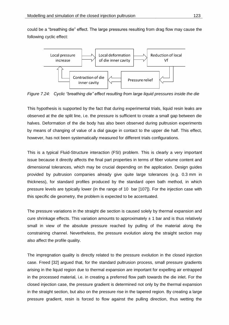
Modelling and simulation of the closed injection pultrusion 123
could be a “breathing die” effect. The large pressures resulting from drag flow may cause the
following cyclic effect:
Figure 7.24: Cyclic “breathing die” effect resulting from large liquid pressures inside the die
This hypothesis is supported by the fact that during experimental trials, liquid resin leaks are
observed at the die split line, i.e. the pressure is sufficient to create a small gap between die
halves. Deformation of the die body has also been observed during pultrusion experiments
by means of changing of value of a dial gauge in contact to the upper die half. This effect,
however, has not been systematically measured for different trials configurations.
This is a typical Fluid-Structure interaction (FSI) problem. This is clearly a very important
issue because it directly affects the final part properties in terms of fiber volume content and
dimensional tolerances, which may be crucial depending on the application. Design guides
provided by pultrusion companies already give quite large tolerances (e.g. 0.3 mm in
thickness), for standard profiles produced by the standard open bath method, in which
pressure levels are typically lower (in the range of 10 bar [107]). For the injection case with
this specific die geometry, the problem is expected to be accentuated.
The pressure variations in the straight die section is caused solely by thermal expansion and
cure shrinkage effects. This variation amounts to approximately ± 1 bar and is thus relatively
small in view of the absolute pressure reached by pulling of the material along the
constraining channel. Nevertheless, the pressure evolution along the straight section may
also affect the profile quality.
The impregnation quality is directly related to the pressure evolution in the closed injection
case. Freed [32] argued that, for the standard pultrusion process, small pressure gradients
arising in the liquid region due to thermal expansion are important for expelling air entrapped
in the processed material, i.e. in creating a preferred flow path towards the die inlet. For the
closed injection case, the pressure gradient is determined not only by the thermal expansion
in the straight section, but also on the pressure rise in the tapered region. By creating a large
pressure gradient, resin is forced to flow against the pulling direction, thus wetting the

124 Modelling and simulation of the closed injection pultrusion
reinforcement stack. Figure 7.25 shows a plot of the pressure gradient at the center line
against the x-position for the trial configuration 1. Below the plot, the corresponding region is
displayed as a pressure contour plot together with vector arrows corresponding to the local
pressure gradients. The x-axis scales of the graph and the contour plot are aligned; the out-
of-plane axis of the contour plot is scaled up for visualization purposes.
Figure 7.25: Top: center line pressure and pressure gradient plot for trial configuration 1;
bottom: pressure contour plot and vector arrows indicating local pressure
gradients
It can be seen that the pressure gradient reaches a maximum shortly before the transition
edge (x = 480 mm). It is expected that entrapped air will flow against the pressure gradient
vector, i.e. in the direction of pressure decrease. This process is facilitated in the tapered
region between approximately 350 mm distance from the die inlet up to the transition to the
curing section of the die. In the region immediately after the transition, it is expected that
further air release is hindered due to a slight pressure decrease after reaching a maximum at
the transition edge. This can also be seen by the vector arrows pointing to the left direction
between 500 mm and 550 mm. One way to improve air release also in the straight section
would be to optimize the positioning of heating plates and/or remove or reduce the cooling
power, such that thermal expansion would lead to further pressure increase immediately
after the transition conical-straight. However, such a modification of the trial assembly would
potentially increase premature curing of resin in the tapered section, and thus reduce
processing stability.

Modelling and simulation of the closed injection pultrusion 125
7.2.2.3 Flow behavior in the tear drop impregnation section
The tear drop cavity has a more complex geometry, and no previous publication containing a
corresponding modelling attempt has been found during the literature research. The
simulation results for trial configuration 8 are shown in Figure 7.26. The porosity and
permeability as defined according to the different region assignments listed in Table 7.4. For
comparison purposes, another simulation run was conducted by setting the thickness and
permeability of the fiber stack along the impregnation chamber to the same value as in the
inlet and curing sections. The reason for this comparison was to evaluate whether the
simulation setting may be simplified, because in this case a subdivision of porosity and
permeability regions according to Table 7.4 is not necessary. An inlet boundary condition of
1.3 bar constant pressure was set, corresponding to the measured value of pressure
transducer 1.
Figure 7.26: Predicted pressure and pressure gradient along the tear drop die center line for
trial configuration 8 up to the detachment point
The centerline pressure remains practically constant along the injection region up to the point
where the fiber stack is compressed towards the end of the tapered region (see Figure 7.9).
The predicted pressure level at the end of the tapered section is higher than the measured
signal. Comparison of results obtained from the simulation run assuming a constant stack
thickness indicate that the simulation set according to the simpler assumption slightly
underestimates the pressure evolution along the impregnation region.
0 100 200 300 400 500 600 700
0
10
20
30
40
50
60
Pre
ssure
[bar]
x-position from die inlet [mm]
Measured pressure values
Varying stack thickness case
Pressure
Pressure gradient
Constant stack thickness case
Pressure
0
2
4
6
8
10
12
14
Pre
ssure
gra
die
nt [x
10
7 k
g/(
m².
s²)
]

126 Modelling and simulation of the closed injection pultrusion
It can be concluded that the proposed model does not reproduce well the process conditions
observed during experimental trials. A number of factors are likely to play a role in the non-
applicability of the model:
Deformation of the die cavity under liquid pressure. As previously discussed, although the
absolute liquid pressure is lower in comparison to the reached pressure levels within the
conical die, the inner cavity of the tear drop die has twice the width of the conical die and
the die body has a smaller thickness (36 mm each die half vs 45 mm of the conical die).
Insufficient liquid impregnation of the reinforcement material. The model assumes a
single liquid phase and therefore a perfect filling of the liquid portion in the porous
domains. The presence of large dry spots may eventually reduce the pressure level in the
chamber. Support for this supposition is given by the various micrographs, which have as
a general rule shown lots of air pockets (see Figure 6.12 and Figure 6.14).
Inhomogeneous distribution of porosity within the fiber stack. The model assumes a
homogeneous fiber distribution of the fiber stack within the impregnation chamber. This
might represent an oversimplification of the process. The much lower pressure rise
obtained from the simulation assuming a constant stack thickness throughout the whole
die is indication of this hypothesis. It is evident from comparison of both simulation results
and observation of the micrographs that a refined model assuming a porosity gradient
across the stack thickness should deliver more realistic results.
The pressure gradient plot in Figure 7.26 shows a similar trend already seen for the conical
die case. The pressure gradient vectors show a favorable orientation for air release along the
die entrance and the whole impregnation chamber, i.e. towards the die entrance (vectors not
shown).
An important observation made during experimental trials with the tear drop assembly was
the progressive clogging of the die, leading to complete obstruction of the impregnation
chamber after a couple of hours (see Section 6.2.2). This is clear evidence that no steady
state governs the flow of liquid resin within this region, but rather a transient condition
prevails, in which the resin gradually cure at regions with presumably low local velocity. In
other words, the geometric design is not optimized for this combination of fast curing resin
system and processing conditions. Observation of the 3D flow field obtained from a steady
state simulation provides insight of stagnation regions. Contour plots of a cross section at a
position x = 116 mm from the die inlet, i.e. the location of the injection ports, and a
longitudinal view are given in the following Figures. The plots were reflected over the XY
plane for visualization purposes.
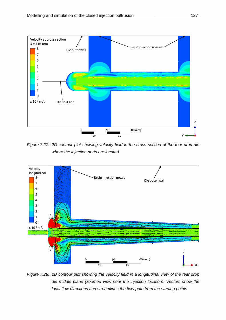
Modelling and simulation of the closed injection pultrusion 127
Figure 7.27: 2D contour plot showing velocity field in the cross section of the tear drop die
where the injection ports are located
Figure 7.28: 2D contour plot showing the velocity field in a longitudinal view of the tear drop
die middle plane (zoomed view near the injection location). Vectors show the
local flow directions and streamlines the flow path from the starting points

128 Modelling and simulation of the closed injection pultrusion
Low local velocities are found in the regions near the tapered wall but also in the bulk of the
fluid region. In the longitudinal plot, the neat resin region between the moving fiber stack and
the tapered die wall can be clearly discerned as a backflow region. The region around the
injection ports is characterized by swirling. The large diameter of the injection ports results in
a stagnation volume with very low velocities. From this steady state result, the flow path and
residence times for particles located in defined positions can be calculated. The flow path is
shown by streamlines for five starting points located at x = 116 mm and different heights. It
can be seen that the fluid can cover a large distance along the tapered section and flow back
to the inlet region. It should be noted that the fluid flow within the impregnation region
actually has a 3D pattern. The 2D representation in Figure 7.28 solely provides an easier
visualization and physically only makes sense at the symmetry plane considered.
According to the flow paths described above, the particles are submitted to a specific
temperature and consequently a curing history. Another way of evaluating the effect of
stagnation regions on local curing would be to run transient simulations; however, such a
transient analysis is not included in this work.
7.2.3 Parametrization of geometric design
In order to explore the impact of processing parameters and geometric design features on
simulation predictions, a number of parametrization studies was conducted. For the conical
die, the effect of varying the heat input / output to the die was analyzed, as well as the pulling
speed. In terms of geometric design, the conical angle was varied, and simulated under the
non-homogeneous porosity distribution assumption (see Figure 7.6). Additionally, the impact
of die body thickness on the thermal balance was evaluated.
For the tear drop die, focus was given to modifying the chamber design in order to obtain
less stagnation regions, i.e. to avoid low velocity pockets. The position and diameter of the
injection nozzles, the length and tapering angle of the chamber were simulated in this case.
The impact of variations in the heat input to the die were evaluated modifying the base case
(see Figure 7.17) by the following two scenarios: (1) removal of the cooling zone and (2)
removal of the cooling zone, increase of the heat input by 30% in heating zones 1 and 4 and
reduction of the heat output by 30% in heating zones 2 and 3. Comparison of these two
scenarios with the base case is shown in Figure 7.29.

Modelling and simulation of the closed injection pultrusion 129
Removal of the cooling zone leads to a slight increase in temperature and degree of cure at
the intersection between tapered and straight regions. This is however, according to the
simulation, uncritical. The increase of heat input, on the other hand, results in an overall
higher temperature plateau in the range of 130 – 140 °C and triggering of the second
reaction step towards the end of the die. This is considered as an unstable processing
condition, especially because the heat release from the curing reaction is expected to
promote curing also after the material is pulled out of the die.
Figure 7.29: Comparison between simulation results of the conical die with different
scenarios in terms of heat input / output to the die
The issue of the die inner cavity deformation, which has been discussed in Section 7.2.2.2,
may in principle be minimized or eliminated by designing the die with thicker body halves.
The original die half thickness of 45 mm was increased by 10% and 50% for comparison
purposes. The results of temperature evolution along the die length from steady state
simulations are plotted in Figure 7.30.
It can be stated that increasing the die body thickness is advantageous both in terms of
reducing the cavity deformation as well as in terms of thermal management. By increasing
the die thickness by 50%, the exothermic peak located between the first and second heating
zones is distinctly reduced, i.e. the additional body mass is able to absorb more effectively
the released reaction heat. On the other hand, the effect on the conversion progress is
almost negligible. A slightly slower degree of cure evolution can be seen, and the curves
approach the same plateau corresponding to the B-stage towards the end of the die. It
0 200 400 600 800 1000 1200 1400 1600
20
40
60
80
100
120
140
x-position from die inlet [mm]
Temperature
Base case
Cooling zone disabled
30% increased heat input
Tem
pera
ture
[°C
]
0.0
0.2
0.4
0.6
0.8
1.0
Degree of cure
Base case
Cooling zone disabled
30% increased heat input
Degre
e o
f cure

130 Modelling and simulation of the closed injection pultrusion
should be noted, however, that these results are based on steady state simulations. If one
considers a process with varying temperature set points, a die with larger body mass is
expected to take longer to reach a new steady state after changing the temperature setting.
This should however not represent a limitation for pultrusion, which is supposed to run on
stationary conditions.
Figure 7.30: Comparison between thermal simulations results of the conical die with different
die body thicknesses
Increasing the pulling speed is usually desired as a means to increase productivity. It is
expected that the pulling speed will have a significant impact on the pressure rise within the
tapered section. The effect of the pulling speed in the curing reaction evolution was
evaluated by two simulations. On scenario 1, the pulling speed was increased to 0.5 m/min
and the heat exchange through the cooling and heating zones was kept as the base case.
On scenario 2, the heat input through the heating zones was changed in order to obtain the
set temperature of 100 °C on the control TC corresponding to zones 1 through 3. The
resulting curves of temperature, degree of cure and viscosity evolution along the center line
are shown in Figure 7.31.
0 200 400 600 800 1000 1200 1400 1600
20
40
60
80
100
120
x-position from die inlet [mm]
Temperature
Base case
Half-thickness 49.5 mm
Half-thickness 67.5 mm
Tem
pera
ture
[°C
]
0.0
0.2
0.4
0.6
0.8
1.0
Degree of cure
Base case
Half-thickness 49.5 mm
Half-thickness 67.5 mm
Degre
e o
f cure
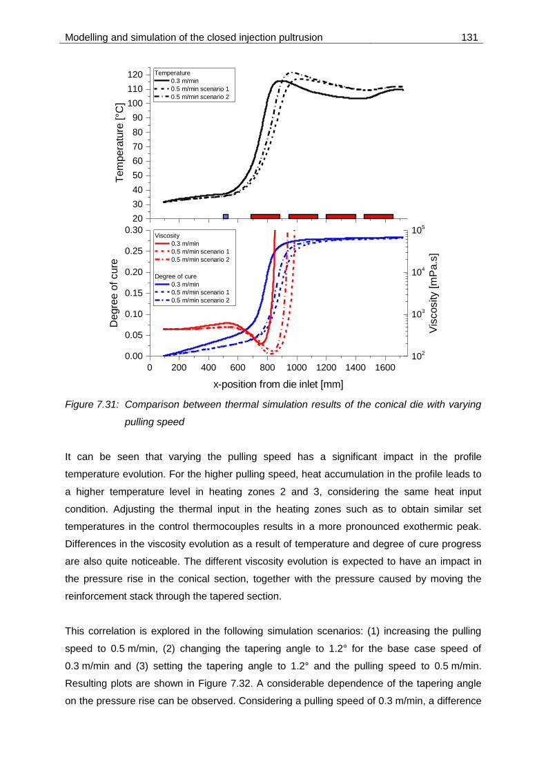
Modelling and simulation of the closed injection pultrusion 131
Figure 7.31: Comparison between thermal simulation results of the conical die with varying
pulling speed
It can be seen that varying the pulling speed has a significant impact in the profile
temperature evolution. For the higher pulling speed, heat accumulation in the profile leads to
a higher temperature level in heating zones 2 and 3, considering the same heat input
condition. Adjusting the thermal input in the heating zones such as to obtain similar set
temperatures in the control thermocouples results in a more pronounced exothermic peak.
Differences in the viscosity evolution as a result of temperature and degree of cure progress
are also quite noticeable. The different viscosity evolution is expected to have an impact in
the pressure rise in the conical section, together with the pressure caused by moving the
reinforcement stack through the tapered section.
This correlation is explored in the following simulation scenarios: (1) increasing the pulling
speed to 0.5 m/min, (2) changing the tapering angle to 1.2° for the base case speed of
0.3 m/min and (3) setting the tapering angle to 1.2° and the pulling speed to 0.5 m/min.
Resulting plots are shown in Figure 7.32. A considerable dependence of the tapering angle
on the pressure rise can be observed. Considering a pulling speed of 0.3 m/min, a difference
0 200 400 600 800 1000 1200 1400 1600
0.00
0.05
0.10
0.15
0.20
0.25
0.30
Degree of cure
0.3 m/min
0.5 m/min scenario 1
0.5 m/min scenario 2
Degre
e o
f cure
x-position from die inlet [mm]
20
30
40
50
60
70
80
90
100
110
120 Temperature
0.3 m/min
0.5 m/min scenario 1
0.5 m/min scenario 2
Tem
pera
ture
[°C
]
102
103
104
105
Viscosity
0.3 m/min
0.5 m/min scenario 1
0.5 m/min scenario 2
Vis
cosity [m
Pa.s
]
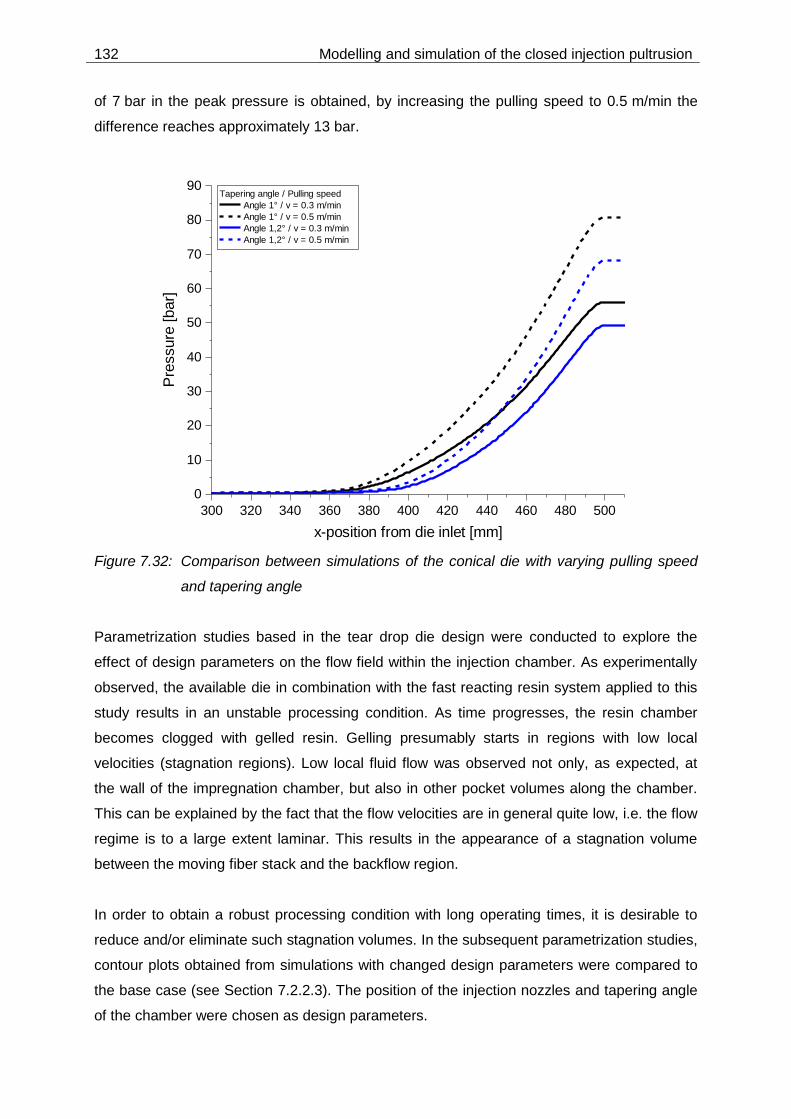
132 Modelling and simulation of the closed injection pultrusion
of 7 bar in the peak pressure is obtained, by increasing the pulling speed to 0.5 m/min the
difference reaches approximately 13 bar.
Figure 7.32: Comparison between simulations of the conical die with varying pulling speed
and tapering angle
Parametrization studies based in the tear drop die design were conducted to explore the
effect of design parameters on the flow field within the injection chamber. As experimentally
observed, the available die in combination with the fast reacting resin system applied to this
study results in an unstable processing condition. As time progresses, the resin chamber
becomes clogged with gelled resin. Gelling presumably starts in regions with low local
velocities (stagnation regions). Low local fluid flow was observed not only, as expected, at
the wall of the impregnation chamber, but also in other pocket volumes along the chamber.
This can be explained by the fact that the flow velocities are in general quite low, i.e. the flow
regime is to a large extent laminar. This results in the appearance of a stagnation volume
between the moving fiber stack and the backflow region.
In order to obtain a robust processing condition with long operating times, it is desirable to
reduce and/or eliminate such stagnation volumes. In the subsequent parametrization studies,
contour plots obtained from simulations with changed design parameters were compared to
the base case (see Section 7.2.2.3). The position of the injection nozzles and tapering angle
of the chamber were chosen as design parameters.
300 320 340 360 380 400 420 440 460 480 500
0
10
20
30
40
50
60
70
80
90
Pre
ssure
[bar]
x-position from die inlet [mm]
Tapering angle / Pulling speed
Angle 1° / v = 0.3 m/min
Angle 1° / v = 0.5 m/min
Angle 1,2° / v = 0.3 m/min
Angle 1,2° / v = 0.5 m/min

Modelling and simulation of the closed injection pultrusion 133
Simulation results for the tear drop die design replicating the actual die geometry has shown
that the injection nozzle diameter is too large, resulting in a stagnation region and backflow
as seen in Figure 7.28. In the following simulations, the nozzle diameter was reduced to
6 mm.
The velocity field in the longitudinal middle plane is shown for a case in which the tapering
angle was reduced to 1° (against the base case angle of 1.2°) in Figure 7.33. An inlet
boundary condition of constant pressure of 1.3 bar was set. A discontinuity is discernible in
the velocity field at the position x = 200 mm from the die inlet. This is due to the interface
between the domains 4 (with hexagonal elements) and 5 (with tetrahedral elements) (see
Figure 7.4). For the base case, the effect of this interface is much less pronounced.
However, the influence of this discontinuity may be assumed as negligible for the purpose of
comparison of the flow fields.
Figure 7.33: 2D contour plot showing velocity field in a longitudinal view of the tear drop die
middle plane (zoomed view near the injection location) for a case with tapering
angle of 1°
Comparison between Figure 7.33 and Figure 7.28 reveals a marginal changing of the
velocity field near the nozzle channel discharge. Low velocity regions can still be found along
the cavity, however, due to the reduced free volume between the reinforcement stack and
the cavity inner walls, the overall stagnation volume is reduced.
The velocity field in the longitudinal middle plane is shown for three cases with different
injection nozzle locations in Figure 7.34. In all cases the same inlet boundary condition of
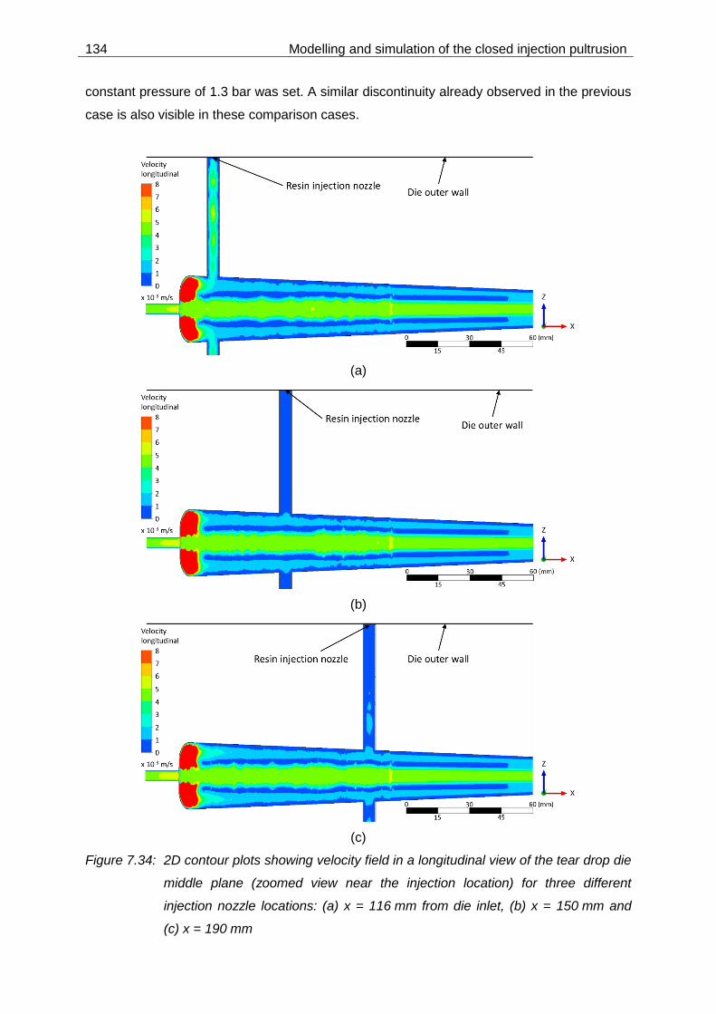
134 Modelling and simulation of the closed injection pultrusion
constant pressure of 1.3 bar was set. A similar discontinuity already observed in the previous
case is also visible in these comparison cases.
(a)
(b)
(c)
Figure 7.34: 2D contour plots showing velocity field in a longitudinal view of the tear drop die
middle plane (zoomed view near the injection location) for three different
injection nozzle locations: (a) x = 116 mm from die inlet, (b) x = 150 mm and
(c) x = 190 mm

Modelling and simulation of the closed injection pultrusion 135
It can be stated that changing nozzle position along the x axis has little influence in the flow
field within the impregnation chamber itself; however, the flow within the nozzle channel is
influenced. By maintaining the nozzle in its original position (Figure 7.34 (a)), higher
velocities are reached than in the comparing cases (b) and (c). This is possibly due to the
fact that a vortex region is located close to the nozzle discharge, a condition which was
already observed for the base case. It can be concluded that a reduction of the nozzle
diameter would be advantageous in increasing local velocities and therefore reducing the risk
of channel obstruction. On the other hand, the impact of designing the injection nozzles
downstream of the base case position may be considered as negligible.
136 Conclusions and outlook
8 Conclusions and outlook
In this thesis, a holistic approach to the simulation of physical processes involved in
pultrusion dies with a closed injection and impregnation cavity was developed. Most
previously published studies have focused in only one aspect of such physical processes, i.e.
reaction kinetics and energetics evolution (thermo-chemical approach), fluid dynamics or
evolution of internal stress and distortions throughout curing (thermo-mechanical approach).
Specifically, in this study, the thermo-chemical model is applied to obtain a more realistic
prediction of the viscosity of the resin while it cures, i.e. coupling of the thermo-chemical and
fluid dynamics model. Furthermore, the thermo-chemical and thermo-mechanical models are
coupled to obtain a prediction of liquid pressure in the curing section of the die up to the point
where the resin gels.
Different experimental characterization techniques were employed to obtain reliable material
data to feed the simulation models. A fast reacting, two-step-curing resin system was
characterized in terms of reaction kinetics by DSC and the viscosity evolution throughout
curing was determined by rheology measurements. For this resin system, it was shown that
taking into account the viscosity evolution is essential for obtaining realistic predictions for
the flow behavior. The kinetics of the first reaction step leading to a B-stage intermediate
product is rather fast, leading to a considerable conversion while the material is still in the
injection and impregnation chamber. This, in turn, causes changes in the material viscosity.
Simulation results for the pressure rise obtained by incorporating a varying viscosity agreed
better with experimental results than results obtained under a constant viscosity assumption.
Reinforcement materials were characterized in terms of their compressibility, i.e. the elastic
response of a fiber stack to a transverse mechanical load, and in-plane permeability. For the
compressibility, reproducible results could be obtained for glass continuous filament mats,
and stacks composed of glass fiber and carbon fiber rovings. It was argued that determining
the compressibility of reinforcements is important for the process simulation of cases in
which different materials are applied, e.g. a combination of CFM and roving layers. In such
cases, the fiber volume content of each layer cannot be determined from the cavity cross
section alone, it is rather a function of the mechanical pressure applied to the whole
reinforcement stack.
The results for the experimental permeability characterization were less consistent. This
material parameter is extremely sensitive to the fiber volume fraction. The developed method
for in-plane characterization delivered results comparable to the literature in the case of
Conclusions and outlook 137
planar textiles. The determination of the permeability of roving stacks was, on the other hand,
challenging due to the narrow range of measurable fiber volume fractions, in which a very
restricted saturated flow takes place. The permeability along the fiber orientation agreed
reasonably well with Gebart’s theoretical model, while values for the traverse permeability
were considerably lower than theoretically predicted for the same fiber volume content.
Simulation studies comparing different permeability values showed that the flow field and
pressure rise is very sensitive to the longitudinal permeability, but are practically not
influenced by the transverse permeability.
Two pultrusion dies with different closed injection and impregnation chambers were modelled
and simulated: one with a conical inlet geometry and another with a so-called tear drop
injection and impregnation chamber. Experimental trials were conducted with both die
assemblies in order to compare simulation results with real processing data.
The simulation model needs the definition of the porosity within the domain corresponding to
the fiber stack over a broad range of fiber volume content. Two models were proposed for
the case of the conical die: a simplified model assuming a homogeneous fiber distribution
over the whole cavity cross section, and a model accounting for an inhomogeneous
distribution of the reinforcement within the cross section.
The simulation results for the pressure rise in a conical injection chamber agree well with
experimentally determined pressures for different fiber volume contents. This gives
confidence in the validity of the developed model. The conical geometry study causes a
pressure rise of the order of magnitude of 50 bar. Such a liquid pressure is expected to
account for a considerable fraction of the pulling force. The direct correlation of measured
pulling force and pressure signals is also indication of this behavior.
The predicted pressure rise is not in good agreement with experimental processing data in
the case of the tear drop chamber, i.e. the predicted liquid pressure at the beginning of the
straight curing section is higher. The discrepancy was attributed to a combination of different
factors: deformation of the die cavity under liquid pressure, insufficient impregnation of the
reinforcement stack and an oversimplification of the fiber stack distribution assumption.
Future work in this topic could include a coupling of the flow field with an elastic deformation
model of the die body (Fluid-Structure Interaction). Since the high liquid pressures are, in
contrast to the conventional pultrusion technique, characteristic of the closed injection
pultrusion, a possible deformation of the die body should be considered in the simulation.

138 Conclusions and outlook
The importance of such an approach is justified by the high sensitivity of the permeability to
variations in the die cavity and, consequently, in the fiber volume content.
Furthermore, efforts should be undertaken to study the correlation of the liquid pressure level
and/or pressure gradient with the impregnation quality. In other words, the optimization of
pressure rise or pressure gradient function should be sought. In general, a relatively low
pressure level on the order of 10 – 20 bar would be preferable than 50 – 60 bar, which could
be easily obtained by designing a slightly larger tapering angle. The question as to which
pressure level and/or pressure increase rate is necessary to obtain a satisfactory
impregnation quality can only be addressed by an extensive characterization study on
pultruded profiles produced under different dies and processing conditions.
The fast reacting resin system applied to this study does not allow for stable processing with
the tear drop die. This is due to the relatively large impregnation cavity volume, which
creates stagnation regions, i.e. regions with low flow velocities. In combination with the
curing kinetics, this leads to a progressive clogging of the chamber with gelled resin. It has
been shown that, by reducing the injection nozzle diameter and the conical angle, and
thereby the chamber volume, a more favorable flow field can be obtained, i.e. the stagnation
volume is reduced. A more detailed study of this die design would demand the conduction of
transient simulation studies, to obtain a prediction of the viscosity field in the impregnation
chamber and of incipient gelling regions.
In this study, a commercial CFD software was applied, with results comparable to previous
self-written simulation codes described in the literature, as was proven in comparing studies
for simplified 1D/2D geometries. Considering the possibility of implementing complex
geometric models, the present simulation model can be a useful tool in studying other
impregnation chamber geometries and/or profile cross sections. The application of a
commercial package also facilitates the potential use in an industrial environment, as a
support tool for the design of pultrusion dies with closed injection and impregnation
chambers.

Appendix 139
Appendix
Appendix A: Processing data from pultrusion experimental trials
Table A.1: Processing data from trials with the conical die
Trial number
1 2 3 4 5 6
Fiber stack GF GF GF CF CF CF
Pulling speed [m/min] 0.3 0.3 0.3 0.5 0.3 0.3
Fiber volume content [%] 0.64 0.6 0.57 0.64 0.64 0.6
Set Temperature [°C] 100 100 100 100 100 100
TC1 [°C] 100 100 100 100 100 100
TC2 [°C] 101 101 101 100 100 100
TC3 [°C] 100 100 100 100 100 100
TC4 [°C] 100 100 100 100 100 100
TC5 [°C] 30 31 31 26 27 27
TC6 [°C] 111 111 111 111 111 111
TC7 [°C] 104 104 104 103 103 103
TC8 [°C] 100 100 100 100 100 100
TC9 [°C] 100 100 100 100 100 100
TC10 [°C] 101 100 100 99 99 100
TC11 [°C] 102 102 101 101 100 100
Electrical power, Zone 1 [%] 46.0 ± 5.9 46.2 ± 4.5 46.6 ± 5.0 52.1 ± 5.6 41.6 ± 7.0 44.1 ± 6.2
Electrical power, Zone 2 [%] 1.4 ± 2.9 1.2 ± 2.9 1.9 ± 3.8 1.2 ± 3.1 2.4 ± 4.1 1.9 ± 3.2
Electrical power, Zone 3 [%] 7.2 ± 3.9 7.5 ± 3.3 7.7 ± 3.4 7.4 ± 3.5 8.2 ± 3.6 7.7 ± 2.9
Electrical power, Zone 4 [%] 12.8 ± 5.6 13.1 ± 3.8 13.9 ± 3.9 15.3 ± 6.7 16.8 ± 4.6 17.2 ± 3.2
Pulling force [kN] 12.1 ± 1.5 8.4 ± 1.7 7.7 ± 1.2 1.9 ± 0.2 2.7 ± 1.0 2.8 ± 0.8
Resin injection pressure [bar] 0.4 * 0.4 * 0.4 * 0.4 * 0.4 * 0.4 *
Pressure transducer 1 [bar] 8.9 ± 0.9 5.1 ± 1.2 3.2 ± 0.6 0 0 0
Pressure transducer 2 [bar] 51.9 ± 5.3 33.7 ± 6.4 23.7 ± 2.1 5.9 ± 1.4 7.6 ± 5.7 16.7 ± 4.4
* Resin is injected intermittently.

140 Appendix
Table A.2: Processing data from trials with the tear drop die
Trial number
7 8 9 10
Fiber stack GF GF GF GF
Pulling speed [m/min] 0.5 0.3 0.3 0.3
Fiber volume content [%] 0.64 0.64 0.6 0.64
Set Temperature [°C] 100 100 100 80
TC1 [°C] 100 100 100 80
TC2 [°C] 102 101 100 82
TC3 [°C] 100 100 100 80
TC4 [°C] 17 17 17 21
TC5 [°C] 50 52 53 47
TC6 [°C] 106 106 106 84
TC7 [°C] 105 104 103 83
TC8 [°C] 102 102 101 79
TC9 [°C] 98 98 98 76
Electrical power, Zone 1 [%] 34.1 ± 4.0 25.8 ± 5.0 26.7 ± 6.0 18.2 ± 4.6
Electrical power, Zone 2 [%] 1.5 ± 3.2 2.3 ± 3.8 2.2 ± 4.1 2.2 ± 4.2
Electrical power, Zone 3 [%] 7.1 ± 7.1 6.9 ± 3.9 6.7 ± 3.1 3.7 ± 2.9
Pulling force [kN] 2.1 ± 0.1 3.9 ± 0.2 2.5 ± 0.2 2.8 ± 0.2
Resin injection pressure [bar] 2.3 ± 0.1 3.4 ± 0.7 1.5 ± 0.2 3.0 ± 0.8
Pressure transducer 1 [bar] 0 1.3 ± 0.7 0 1.1 ± 0.7
Pressure transducer 2 [bar] 11.7 ± 1.0 14.5 ± 0.8 7.6 ± 0.5 13.3 ± 0.9

Appendix 141
Appendix B: Mesh quality parameters of the tear drop die 3D model
Region Number of
nodes Number of elements
Average skewness
factor
Elements with
skewness > 0.75 [%]
1 55146 45000 1.3 x 10⁻¹⁰ 0
2 224406 184500 1.6 x 10⁻¹⁰ 0
3 29484 23850 8.1 x 10⁻³ 0
4 91728 75150 8.1 x 10⁻³ 0
5 94071 488474 0.31 0.46
6 16973 80297 0.26 0.47
7 655165 3538915 0.24 0.76

142 Appendix
Appendix C: Analytical model for the pressure rise in a conical inlet section
The analytical models proposed by Kim et al. [27] and Ding et al. [10] for the pressure rise
function in a conical die inlet, which are based on a 1D flow assumption were found to agree
well with simulations in a 2D field. It has also been shown that the analytical model can be
generalized to an injection port located at a determined position along the tapered section.
An explicit formulation for the pressure rise along the conical inlet section is derived in this
appendix. It should be noted that the analytical solution is valid for a unidirectional fiber stack
only, because the permeability is expressed as a smooth function of the tapering geometry.
Ding derived from the mass conservation and Darcy’s laws the following relationships for the
pressure gradients due to drag flow and flow driven by the injection pressure. Refer to Figure
7.5 for the geometrical parameters defined in the equations.
𝑑𝑃𝐷
𝑑𝑥= −
𝐶𝐺 ∙ 𝜂 ∙ 𝑈 ∙ 𝑉𝑓2 ∙ ℎ𝑐
2
𝐷𝑓2 ∙
(𝐿 − 𝑥) tan 𝜃
[(1 − 𝑉𝑓)ℎ𝑐 + 2(𝐿 − 𝑥) tan 𝜃]3 Equation B.1
𝑑𝑃𝑝
𝑑𝑥= −
𝐶𝐺 ∙ 𝜂 ∙ 𝑈 ∙ 𝑉𝑓2 ∙ ℎ𝑐
2
2𝐷𝑓2 ∙
(1 − 𝑉𝑓)ℎ𝑐
[(1 − 𝑉𝑓)ℎ𝑐 + 2(𝐿 − 𝑥) tan 𝜃]3 Equation B.2
Where 𝑃𝐷 and 𝑃𝑃 are the pressure distributions due to drag flow and due to the injection
pressure, respectively. 𝐷𝑓 is the filament diameter and 𝐶𝐺 is the shape factor defined by
Gebart, with value 57 for a quadratic fiber arrangement. It should be noted that Equation B.1
is exactly the same as Equation 3.30 by neglecting volume change effects. Integration of the
above equations yields:
𝑃𝐷 = 𝐴 ∙ [
1 + 2휀
2(1 + 휀)2] + 𝐶1 Equation B.3
𝑃𝑃 = 𝐴 ∙ [
1
2(1 + 휀)2] + 𝐶2 Equation B.4
With 𝐴 and 휀 defined as:
𝐴 =
𝐶𝐺 ∙ 𝜂 ∙ 𝑈 ∙ ℎ𝑐 ∙ 𝑉𝑓2
4𝐷𝑓2 ∙ tan 𝜃 (1 − 𝑉𝑓)
Equation B.5

Appendix 143
휀 =
2(𝐿 − 𝑥) tan 𝜃
(1 − 𝑉𝑓)ℎ𝑐
Equation B.6
Assuming a location port at a position 𝑥𝑖𝑛 within the conical section where resin is injected
under pressure 𝑃𝑖𝑛, the integration constants 𝐶1 and 𝐶2 can be determined by considering
that at this location the superposed flow function, which is valid upstream of the port, equals
the downstream drag flow, i.e. 𝑃𝐷 = 𝑃𝐷 + 𝑃𝑃, leading to:
𝑃𝐷 = 𝑃𝑖𝑛 → 𝐶1 = 𝑃𝑖𝑛 − 𝐴 [
1 + 2휀𝑖𝑛
2(1 + 휀𝑖𝑛)2] Equation B.7
𝑃𝑝 = 0 → 𝐶2 = −𝐴 [
1
2(1 + 휀𝑖𝑛)2] Equation B.8
Where 휀𝑖𝑛 is the value of 휀 calculated at 𝑥𝑖𝑛. By substituting the integration constants in
Equations B.3 and B.4, we arrive at the general pressure function for the conical inlet
section:
𝑃 = 𝑃𝑖𝑛 + 𝐴 [
1
1 + 휀−
1
1 + 휀𝑖𝑛] , 0 ≤ 𝑥 ≤ 𝑥𝑖𝑛 Equation B.9
𝑃 = 𝑃𝑖𝑛 + 𝐴 [
1 + 2휀
2(1 + 휀)2−
1 + 2휀𝑖𝑛
2(1 + 휀𝑖𝑛)2] , 𝑥𝑖𝑛 ≤ 𝑥 ≤ 𝐿 Equation B.10

144 References
References
[1] R. Bezerra, F. Wilhelm, S. Strauß and H. Ahlborn, "Manufacturing of Complex Shape
Composite Parts through the Combination of Pull-braiding and Blow-Moulding," in 20th
International Conference on Composite Materials, Copenhagen, 2015.
[2] L. Herbeck, Anforderungen an eine Faserverbund-Produktionstechnik, DLR, Ed.,
Braunschweig, 2009.
[3] S. Bühler, "PulPress - Large scale production of complex sandwich profiles," in 13th
World Pultrusion Conference, Prague, 2016.
[4] T. F. Starr, Pultrusion for engineers, Boca Raton, FL: CRC Press, 2000.
[5] "Pultrusion | Fiberline Composites," [Online]. Available: http://fiberline.com/pultrusion.
[Accessed 29 1 2016].
[6] C. Koppernaes, S. G. Nolet and J. P. Fanucci, "Method and apparatus for wetting fiber
reinforcements with matrix materials in the pultrusion process using continuous in-line
degasing". United States Patent 5,073,413, 1991.
[7] J. V. Gauchel and R. N. Lehman, "Apparatus for resin impregnated pultrusion". United
States Patent 5,747,075, 1998.
[8] R. J. Brown, S. Kharchenko, H. D. Coffee and I. Huang, "System for producing
pultruded components". United States Patent 8,597,016, 2013.
[9] M. G. Dubé, G. L. Batch, J. H. Vogel and C. W. Macosko, "Reaction Injection Pultrusion
of thermoplastic and thermoset Composites," Polymer Composites, vol. 16, no. 5, p.
378–385, 1995.
[10] Z. Ding, S. Li, H. Yang, J. L. Lee, H. Engelen and P. M. Puckett, "Numerical and
experimental analysis of resin flow and cure in resin injection pultrusion (RIP)," Polymer
Composites, vol. 21 (5), pp. 762-778, 2000.
[11] M. Connolly, M. Brennan and T. Shidaker, "CFD Modeling of the Closed Injection Wet-
Out Process For Pultrusion," in EPTA's 2008 World Pultrusion Conference, 2008.
[12] S. Li, L. Xu, Z. Ding, L. J. Lee and H. Engelen, "Experimental and Theoretical Analysis
of Pulling Force in Pultrusion and Resin Injection Pultrusion (RIP)-Part I: Experimental,"
Journal of Composite Materials, vol. 37 (2), pp. 163-189, 2003.
[13] D. Srinivasagupta, S. Potaraju, J. L. Kardos and B. Joseph, "Steady state and dynamic
analysis of a bench-scale injected pultrusion process," Composites Part A: Applied
Science and Manufacturing, vol. 34, no. 9, p. 835–846, 2003.
[14] H. Engelen, "Development and Comparison of Resin Injection and Impregnation
Chambers for Pultrusion," in 11th World Pultrusion Conference, Istanbul, 2012.

References 145
[15] J. K. Gillham, "Formation and Properties of Thermosetting and High Tg Polymeric
Materials," Polymer Engineering and Science, pp. 1429-1433, 26 November 1986.
[16] P. J. Halley and M. E. Mackay, "Chemorheology of thermosets - an overview," Polymer
Engineering & Science, vol. 36, no. 5, pp. 593-609, 1996.
[17] A. Yousefi, P. G. Lafleur and R. Gauvin, "Kinetic studies of thermoset cure reactions: A
review," Polymer Composites, vol. 18, no. 2, pp. 157-168, 1997.
[18] M. R. Kamal and S. Sourour, "Kinetics and thermal characterization of thermoset cure,"
Polymer Engineering and Science, vol. 13, no. 1, pp. 59-64, 1973.
[19] M. R. Kamal, "Thermoset characterization for moldability analysis," Polymer
Engineering and Science, vol. 14, no. 3, pp. 231-239, 1974.
[20] W. I. Lee, A. C. Loos and G. S. Springer, "Heat of Reaction, Degree of Cure, and
Viscosity of Hercules 3501-6 Resin," Journal of Composite Materials, vol. 16, no. 6, pp.
510-520, 1982.
[21] I. V. Arkhangel'skii, Non-isothermal kinetic methods, 1. publ ed., vol. 1, Berlin: Ed.
Open Acess, 2013, p. 65 S.
[22] J. Opfermann, "Kinetic Analysis Using Multivariate Non-linear Regression. I. Basic
concepts," Journal of Thermal Analysis and Calorimetry, vol. 60, no. 2, p. 641–658,
2000.
[23] H. L. Price Jr, "Curing and Flow of Thermosetting Resins for Composite Material
Pultrusion," Old Dominion University, 1979.
[24] L. Aylward, G. Douglas and D. Roylance, "A transient finite element model for
pultrusion processing," Polymer Process Engineering, no. 3(3), pp. 247-261, 1985.
[25] G. L. Batch and C. W. Macosko, "Heat Transfer and Cure in Pultrusion: Model and
Experimental Verification," AIChE Journal, vol. 39 (7), pp. 1228-1241, 1993.
[26] C. D. Han and D. S. Lee, "Development of a mathematical model for the pultrusion
process," Polymer Engineering and Science, vol. 26, pp. 393-404, 1986.
[27] D.-H. Kim, P.-G. Han, G.-H. Jin and W. I. Lee, "A Model for Thermosetting Composite
Pultrusion Process," Journal of Composite Materials, vol. 31 (20), pp. 2105-2122, 1997.
[28] S. JOSHI and Y. LAM, "Integrated approach for modelling cure and crystallization
kinetics of different polymers in 3D pultrusion simulation," Journal of Materials
Processing Technology, vol. 174, no. 1-3, pp. 178-182, 2006.
[29] J. Blaurock, "Zur Optimierung des Strangziehverfahrens für endlosfaserverstärkte,
hochfeste Kunststoffprofile," Aachen, 1999.
[30] I. Baran, R. Akkerman and J. H. Hattel, "Material characterization of a polyester resin
system for the pultrusion process," Composites Part B: Engineering, vol. 64, pp. 194-

146 References
201, 2014.
[31] Z. Ding, S. Li and L. J. Lee, "Influence of heat transfer and curing on the quality of
pultruded composites. II: Modeling and simulation," Polymer Composites, vol. 23, no. 5,
pp. 957-969, 2002.
[32] A. D. Freed, "Modelling the pultrusion process to obtain low void fraction composites,"
West Virginia University, 06.05.2002.
[33] S. Li, L. Xu, Z. Ding, L. J. Lee and H. Engelen, "Experimental and Theoretical Analysis
of Pulling Force in Pultrusion and Resin Injection Pultrusion (RIP) - Part II: Modeling
and Simulation," Journal of Composite Materials, vol. 37 (3), pp. 195-216, 2003.
[34] R. M. Hackett and S.-Z. Zhu, "Two-Dimensional Finite Element Model of the Pultrusion
Process," Journal of Reinforced Plastics and Composites, vol. 11, no. 12, pp. 1322-
1351, 1992.
[35] S. Kommu, B. Khomami and J. L. Kardos, "Modeling of injected pultrusion processes: A
numerical approach," Polymer Composites, vol. 19, no. 4, pp. 335-346, 1998.
[36] I. Mustafa, B. Khomami and J. L. Kardos, "3-D nonisothermal flow simulation model for
injected pultrusion processes," AIChE Journal, vol. 45, no. 1, pp. 151-163, 1999.
[37] H. Ng and I. Manas-zloczower, "A nonisothermal differential scanning calorimetry study
of the curing kinetics of an unsaturated polyester system," Polymer Engineering and
Science, vol. 29, no. 16, pp. 1097-1102, 1989.
[38] H. Ng and I. Manas-Zloczower, "Kinetic studies of a composite thermoset cure reaction
- application in pultrusion simulations," Polymer Engineering and Science, vol. 29, no.
5, pp. 302-307, 1989.
[39] S. M. Moschiar, M. M. Reboredo, J. M. Kenny and A. Vázquez, "Analysis of pultrusion
processing of composites of unsaturated polyester resin with glass fibers," Polymer
Composites, vol. 17, no. 3, pp. 478-485, 1996.
[40] R. Gorthala, J. A. Roux and J. G. Vaughan, "Resin Flow, Cure and Heat Transfer
Analysis for Pultrusion Process," Journal of Composite Materials, vol. 28, pp. 486-506,
1994.
[41] R. Gorthala, J. Roux, J. Vaughan and R. Donti, "Comparison of Processing Parameters
for Pultruded Graphite/Epoxy and Fiberglass/Epoxy: A Heat Transfer and Curing
Model," Journal of Reinforced Plastics and Composites, vol. 13, no. 4, pp. 288-300,
1994.
[42] Y. R. Chachad, J. A. Roux, J. G. Vaughan and E. Arafat, "Three-Dimensional
Characterization of Pultruded Fiberglass-Epoxy Composite Materials," Journal of
Reinforced Plastics and Composites, vol. 14, pp. 495-512, 1995.

References 147
[43] Y. R. Chachad, J. A. Roux, J. G. Vaughan and E. S. Arafat, "Effects of Pull Speed on
Die Wall Temperatures for Flat Composites of various Sizes," Journal of Reinforced
Plastics and Composites, no. 15, pp. 718-739, 1996.
[44] Y. R. Chachad, J. A. Roux, J. G. Vaughan and E. S. Arafat, "Thermal Model for Three-
Dimensional Irregular Shaped Pultruded Fiberglass Composites," Journal of Composite
Materials, vol. 30 (6), pp. 692-721, 1996.
[45] M. Valliappan, J. A. Roux and J. G. Vaughan, "Temperature and Cure in Pultruded
Composites Using Multi-Step Reaction Model for Resin," Journal of Reinforced Plastics
and Composites, vol. 15, pp. 295-321, 1996.
[46] M. Valliappan, J. A. Roux, J. G. Vaughan and E. S. Arafat, "Die and post-die
temperature and cure in graphite/epoxy composites," Composites Part B: Engineering,
vol. 27, no. 1, pp. 1-9, 1996.
[47] B. R. Suratno, L. Ye and Y.-W. Mai, "Simulation of temperature and curing profiles in
pultruded composite rods," Composites Science and Technology, vol. 58, no. 2, pp.
191-197, 1998.
[48] X. Lin Liu, I. G. Crouch and Y. C. Lam, "Simulation of heat transfer and cure in
pultrusion with a general-purpose finite element package," Composites Science and
Technology, vol. 60, no. 6, pp. 857-864, 2000.
[49] S. C. Joshi and Y. C. Lam, "Three-dimensional finite-element/nodal-control-volume
simulation of the pultrusion process with temperature-dependent material properties
including resin shrinkage," Composites Science and Technology, vol. 61, pp. 1539-
1547, 2001.
[50] P. Carlone, G. Palazzo and R. Pasquino, "Pultrusion manufacturing process
development by computational modelling and methods," Mathematical and Computer
Modelling, vol. 44, no. 7-8, pp. 701-709, 2006.
[51] P. Carlone, G. Palazzo and R. Pasquino, "Pultrusion manufacturing process
development: Cure optimization by hybrid computational methods," Computers &
Mathematics with Applications, vol. 53, no. 9, pp. 1464-1471, 2007.
[52] J. H. Lee and J. W. Lee, "Kinetic parameters estimation for cure reaction of epoxy
based vinyl ester resin," Polymer Engineering and Science, vol. 34, no. 9, pp. 742-749,
1994.
[53] X. -L. Liu, "Numerical modeling on pultrusion of composite I beam," Composites Part A:
Applied Science and Manufacturing, vol. 32, no. 5, pp. 663-681, 2001.
[54] T. Mezger, Das Rheologie-Handbuch, 3., überarb. Aufl. ed., Hannover: Vincentz
Network, 2010, p. 441 S..

148 References
[55] J. D. Ferry, Viscoelastic properties of polymers, 3d ed ed., New York: Wiley, 1980, pp.
xxiv, 641.
[56] W. P. Cox and E. H. Merz, "Correlation of dynamic and steady flow viscosities," Journal
of Polymer Science, vol. 28, no. 118, pp. 619-622, 1958.
[57] H. H. Winter, "Can the gel point of a cross-linking polymer be detected by theG? -G?
crossover?," Polymer Engineering and Science, vol. 27, no. 22, pp. 1698-1702, 1987.
[58] Test Method for Plastics: Dynamic Mechanical Properties: Cure Behavior, West
Conshohocken, PA, 2008.
[59] J. M. Castro and C. W. Macosko, "Studies of mold filling and curing in the reaction
injection molding process," AIChE Journal, vol. 28, no. 2, p. 250–260, 1982.
[60] T. A. Osswald and N. Rudolph, Polymer rheology, Cincinnati: Hanser Publications,
2015, pp. xi, 225.
[61] T. G. Gutowski, Z. Cai, S. Bauer, D. Boucher, J. Kingery and S. Wineman,
"Consolidation Experiments for Laminate Composites," Journal of Composite Materials,
vol. 21, no. 7, pp. 650-669, 1987.
[62] Y. R. Kim, S. P. McCarthy and J. P. Fanucci, "Compressibility and relaxation of fiber
reinforcements during composite processing," Polymer Composites, vol. 12, no. 1, pp.
13-19, 1991.
[63] G. L. Batch, S. Cumiskey and C. W. Macosko, "Compaction of fiber reinforcements,"
Polymer Composites, vol. 23, no. 3, pp. 307-318, 2002.
[64] R. Arbter et al, "Experimental determination of the permeability of textiles: A benchmark
exercise," Composites Part A: Applied Science and Manufacturing, vol. 42, no. 9, pp.
1157-1168, 2011.
[65] S. Whitaker, "Flow in porous media I: A theoretical derivation of Darcy's law," Transport
in Porous Media, vol. 1, no. 1, pp. 3-25, 1986.
[66] R. B. Bird, W. E. Stewart and E. N. Lightfoot, Transport phenomena, Rev. 2nd ed ed.,
New York: J. Wiley, 2007, pp. xii, 905.
[67] K. L. Adams, W. B. Russel and L. Rebenfeld, "Radial penetration of a viscous liquid
into a planar anisotropic porous medium," International Journal of Multiphase Flow, vol.
14, no. 2, pp. 203-215, 1988.
[68] A. W. Chan and S.-T. Hwang, "Anisotropic in-plane permeability of fabric media,"
Polymer Engineering and Science, vol. 31, no. 16, p. 1233–1239, 1991.
[69] J. R. Weitzenböck, R. A. Shenoi and P. A. Wilson, "Radial flow permeability
measurement. Part A: Theory," Composites Part A: Applied Science and
Manufacturing, vol. 30, no. 6, p. 781–796, 1999.

References 149
[70] J. R. Weitzenböck, R. A. Shenoi and P. A. Wilson, "Radial flow permeability
measurement. Part B: Application," Composites Part A: Applied Science and
Manufacturing, vol. 30, no. 6, p. 797–813, 1999.
[71] K. K. Han, C. W. Lee and P. R. Rice, "Measurements of the permeability of fiber
preforms and applications," Composites Science and Technology, vol. 60, no. 12-13, p.
2435–2441, 2000.
[72] R. Arbter, "Contribution to robust resin transfer molding," ETH, Zürich, 2008.
[73] N. Vernet et al, "Experimental determination of the permeability of engineering textiles:
Benchmark II," Composites Part A: Applied Science and Manufacturing, vol. 61, pp.
172-184, 2014.
[74] B. R. Gebart, "Permeability of Unidirectional Reinforcements for RTM," Journal of
Composite Materials, vol. 26, no. 8, pp. 1100-1133, 1992.
[75] Westhuizen, Josiasvd, Du Plessis, J. Prieur, "Quantification of Unidirectional Fiber Bed
Permeability," Journal of Composite Materials, vol. 28, no. 7, pp. 619-637, 1994.
[76] J. Beckman, R. Lehman, J. Gauchel, R. Werner, Z. Kusibab, J. Kufner and B. Werner,
A Method for Producing Ladder Rail Using High Pressure Injection Die Impregnation,
Owens Corning Technical Paper No. 1-PL-19592, 1995.
[77] P. J. Bates, D. Taylor and M. Cunningham, "Transverse Permeability of Direct Glass
Rovings," Journal of Reinforced Plastics and Composites, vol. 19, no. 15, pp. 1217-
1226, 2000.
[78] J. S. U. Schell, M. Siegrist and P. Ermanni, "Experimental Determination of the
Transversal and Longitudinal Fibre Bundle Permeability," Applied Composite Materials,
vol. 14, no. 2, pp. 117-128, 2007.
[79] J. D. Anderson, Computational fluid dynamics, New York: McGraw-Hill, 1995, pp. xxiv,
547.
[80] S. V. Patankar, Numerical heat transfer and fluid flow, Washington; New York:
Hemisphere Pub. Corp.;McGraw-Hill, 1980, pp. xiii, 197.
[81] Ansys CFX 14.0 Help.
[82] S. U. Gadam, J. A. Roux, T. A. McCarty and J. G. Vaughan, "The impact of pultrusion
processing parameters on resin pressure rise inside a tapered cylindrical die for glass-
fibre/epoxy composites," Composites Science and Technology, vol. 60, pp. 945-958,
2000.
[83] K. S. Raper, J. A. Roux, T. A. McCarty and J. G. Vaughan, "Investigation of the
pressure behavior in a pultrusion die for graphite/epoxy composites," Composites Part
A: Applied Science and Manufacturing, vol. 30 (9), pp. 1123-1132, 1999.

150 References
[84] D. Sharma, T. A. McCarty, J. A. Roux and J. G. Vaughan, "Fluid mechanics analysis of
a two-dimensional pultrusion die inlet," Polymer Engineering & Science, vol. 38, no. 10,
pp. 1611-1622, 1998.
[85] D. Sharma, T. A. McCarty, J. A. Roux and J. G. Vaughan, "Investigation of Dynamic
Pressure Behavior in a Pultrusion Die," Journal of Composite Materials, vol. 32, no. 10,
pp. 929-950, 1998.
[86] D. Sharma, T. A. McCarty, J. A. Roux and J. G. Vaughan, "Pultrusion die pressure
response to changes in die inlet geometry," Polymer Composites, vol. 19 (2), pp. 180-
192, 1998.
[87] I. Baran, C. C. Tutum, M. W. Nielsen and J. H. Hattel, "Process induced residual
stresses and distortions in pultrusion," Composites Part B: Engineering, vol. 51, p. 148–
161, 2013.
[88] T. A. Bogetti and J. W. Gillespie, "Two-Dimensional Cure Simulation of Thick
Thermosetting Composites," Journal of Composite Materials, vol. 25, no. 3, p. 239–
273, 1991.
[89] T. A. Bogetti and J. W. Gillespie, "Process-Induced Stress and Deformation in Thick-
Section Thermoset Composite Laminates," Journal of Composite Materials, vol. 26, no.
5, p. 626–660, 1992.
[90] A. Johnston, R. Vaziri and A. Poursartip, "A Plane Strain Modelfor Process-Induced
Deformationof Laminated Composite Structures," Journal of Composite Materials, vol.
35, no. 16, p. 1435–1469, 2001.
[91] I. Baran, J. H. Hattel, R. Akkerman and C. C. Tutum, "Mechanical Modelling of
Pultrusion Process," Applied Composite Materials, vol. 22, no. 1, p. 99–118, 2015.
[92] I. Baran, R. Akkerman and J. H. Hattel, "Modelling the pultrusion process of an
industrial L-shaped composite profile," Composite Structures, vol. 118, p. 37–48, 2014.
[93] I. Baran, J. H. Hattel and R. Akkerman, "Investigation of process induced warpage for
pultrusion of a rectangular hollow profile," Composites Part B: Engineering, vol. 68, p.
365–374, 2015.
[94] I. Baran, J. H. Hattel, C. C. Tutum and R. Akkerman, "Pultrusion of a vertical axis wind
turbine blade part-II," International Journal of Material Forming, vol. 8, no. 3, p. 367–
378, 2015.
[95] P. Carlone, I. Baran, J. H. Hattel and G. S. Palazzo, "Computational Approaches for
Modeling the Multiphysics in Pultrusion Process," Advances in Mechanical Engineering,
vol. 5, no. 0, p. 301875, 2013.
[96] S. Voorakaranam, B. Joseph and J. L. Kardos, "Modeling and Control of an Injection

References 151
Pultrusion Process," Journal of Composite Materials, vol. 33, no. 13, p. 1173–1204,
1999.
[97] X.-L. Liu, "A finite element/nodal volume technique for flow simulation of injection
pultrusion," Composites Part A: Applied Science and Manufacturing, vol. 34, no. 7, p.
649–661, 2003.
[98] X.-L. Liu, "Iterative and transient numerical models for flow simulation of injection
pultrusion," Composite Structures, vol. 66, no. 1-4, p. 175–180, 2004.
[99] S. S. Rahatekar and J. A. Roux, "Numerical Simulation of Pressure Variation and Resin
Flow in Injection Pultrusion," Journal of Composite Materials, vol. 37, no. 12, p. 1067–
1082, 2003.
[100] S. S. Rahatekar, "Injection Pultrusion Simulation for Polyester/Glass Mat/Rovings/Mat
Composites," Journal of Reinforced Plastics and Composites, vol. 24, no. 1, p. 53–68,
2005.
[101] A. L. Jeswani, J. A. Roux and J. G. Vaughan, "Multiple Injection Ports and Part
Thickness Impact on Wetout of High Pull Speed Resin Injection Pultrusion," Journal of
Composite Materials, vol. 43, no. 19, p. 1991–2009, 2009.
[102] B. K. Ranga, J. A. Roux, J. G. Vaughan and A. L. Jeswani, "Effect of injection chamber
length and pull speed of tapered resin injection pultrusion," Journal of Reinforced
Plastics and Composites, vol. 30, no. 16, p. 1373–1387, 2011.
[103] D. R. Palikhel, J. A. Roux and A. L. Jeswani, "Die-Attached Versus Die-Detached Resin
Injection Chamber for Pultrusion," Applied Composite Materials, vol. 20, no. 1, p. 55–
72, 2013.
[104] "Origin Help," [Online]. Available: http://www.originlab.com/doc/Origin-Help/NLFit-
Theory. [Accessed 14 1 2016].
[105] R. Bezerra, F. Wilhelm and F. Henning, "Compressibility and permeability of fiber
reinforcements for pultrusion," 2014.
[106] F. Wilhelm, "Konzeption, Konstruktion und Erprobung eines Versuchsaufbaus für die
Ermittlung der Permeabilität von Textilhalbzeugen in der Ebene," Karlsruher Institut für
Technologie, Karlsruhe, 13.09.2013.
[107] B. Beck, "Messung der Abzugskräfte im Pultrusionsprozess in Abhängigkeit von
Profildicke und Fasergehalt," Karlsruher Institut für Technologie, Karlsruhe, 30.08.2011.
[108] I. Baran, C. C. Tutum and J. H. Hattel, "The effect of thermal contact resistance on the
thermosetting pultrusion process," Composites Part B: Engineering, vol. 45, no. 1, p.
995–1000, 2013.