modelling and simulation of a bridge interacting with a moving …829478/fulltext01.pdf · the...

Master's Degree Thesis

ISRN: BTH-AMT-EX--2013/D11--SE

Supervisors: Andreas Josefsson, BTH Ansel Berghuvud, BTH

Department of Mechanical Engineering

Blekinge Institute of Technology

Karlskrona, Sweden

2013

Jingrui Yang

Rui Duan

Modelling and Simulation of a Bridge interacting with a moving

Vehicle System

Modelling and Simulation of a

bridge interacting with a moving

vehicle system

Jingrui Yang

Rui Duan

Department of Mechanical Engineering

Blekinge Institute of Technology

Karlskrona, Sweden

2012

Thesis submitted for completion of Master of Science in Mechanical

Engineering with emphasis on Structural Mechanics at the Department of

Mechanical Engineering, Blekinge Institute of Technology, Karlskrona,

Sweden.

1

Abstract:

The problem about the vibration of vehicles and bridge is mainly the

problem of coupling vibration between the vehicles dynamic system and

bridge dynamic system. The vehicles running on the bridge at some

speed can make the bridge vibrate, at the same time the vibration of the

bridge will also affect the vibration of the vehicles. This problem with

interaction and mutual effects is the problem of coupling vibration

between vehicles and bridge.

Because its close relation to practical application it is paid extensive

attention by more and more people. In this thesis we construct the

kinetic model of the bridge subsystem and the vehicle subsystem

separately. Then according to the Euler–Bernoulli beam theory [1], mode

superposition method and D’Alambert principle [2] we get the functions

of the two models. In addition we refer to the relationship of the

geometric on the contact point and the static equilibrium conditions to

construct the relation between the equation of the vehicle vibration and

the equation of bridge vibration. Finally we use MATLAB to write the

code according to the Newmark-beta method [3][4] to handle the

coupled equation.

Keywords:

Vehicles-bridge coupling vibration, Dynamic system, D’Alambert

principle, Euler–Bernoulli beam theory, Mode superposition method,

Newmark-beta method.

2

Acknowledgements

From the selection of topic to the finalization of this thesis, our supervisor

Mr.Andreas Josefsson devoted all his attention to each process. Every detail

of the paper was finished with Mr. Andreas Josefsson’s painstaking care.

We would like to express our grateful acknowledgement to our responsible

and humble supervisor of this thesis, Mr. Andreas Josefsson, for helping,

guiding and encouraging us to complete this thesis. We wish to express our

sincere appreciation to him for helping us check out the thesis and suppose

many constructive suggestions. We also would like to thank our friends

providing technical knowledge and valuable advice whenever we needed

during our research work.

At last we would like to thank all of family members for their unconditional

love and understanding. We are also grateful to all of our friends who

support and motivate us to work hard on the thesis.

3

Contents

Acknowledgements 2

Contents 3

1 Notations 4

2 Introduction 6

2.1 Background 6

2.2 Aim and Scope 7

2.3 Structure of the thesis 7

3 Theoretical modelling 9

3.1 Overview 9

3.2 The kinetic model of the vehicle subsystem 10

3.3 The dynamic model of the bridge subsystem 15

3.4 The compatibility conditions 25

3.5 Construction of complete model 28

4 MATLAB simulation 37

4.1 The influence of the speed 40

4.2 The influence of the bridge’s span 44

4.3 The influence of mass of the vehicle 49

4.4 Verification 54

5 Conclusion and future work 58

5.1 Conclusion 58

5.2 Future work 58

5.2.1 Models and calculation method 58

5.2.2 Numerical method 59

6 References 60

Appendices 61

Appendix A: MATLAB scripts 61

4

1 Notations

vM Mass matrix of vehicle model

vC Damping matrix of vehicle model

vK Stiffness matrix of vehicle model

vy Matrix of the degree of freedom of the vehicle

vF Matrix of exciting force of vibration of the vehicle

E Young's modulus

I Moment of inertia Mass of the beam per unit length Damping coefficient per unit length

,F x t Coupled force on the beam

,by x t Beam’s displacement at the contact point

Dirac function

i x Mode of vibration

i t Modal Coordinates

ciy Displacement of the i’th wheel at the contact point

,b iy x t Displacement of bridge at the i’th contact point

5

,ir x t Irregularity of the bridge’s surface at the i’th point

iW Static load of the wheel and the vehicle body gravity of the

wheel undertake

tiK Stiffness of the tire

tiC Damping of the tire

tiy Displacement the wheel’s middle point in the vertical direction

tiy Velocity of the wheel’s middle point in the vertical direction

ciy Displacement in the vertical direction at the contact point

between the tire and the bridge

ciy Velocity in the vertical direction at the contact point between

the tire and the bridge

6

2 Introduction

2.1 Background

In recent decades, with the rapid development of highway communication

around the world, the increasing number of bridges, the emergence of new

bridge’s structure, the increasing bridge span and a significant increase in

vehicle speed, the research of dynamic interaction between vehicles and the

bridge is more and more intensive. The study of vehicle-bridge coupling

vibration focuses on two aspects generally: accurate modeling of coupled

vehicle-bridge system and efficient methods and algorithms for simulating

the dynamic response.

Figure 2.1. A car is running on a bridge

When the vehicles run across the bridge, the pocket weight of the vehicles,

irregularities of the bridge and the acceleration and braking of the vehicle

can lead to excessive vibrations. The vibration will be transferred to the

bridge by tires, which can make the bridge vibrate forcefully. The bridge

will vibrate in vertical, transverse and longitudinal direction, which could

7

lead to damage in the bridge structure. This problem with interaction and

mutual effects is related to coupled vibrations between the vehicle and the

bridge.

Running vehicles on the bridge at high speed can lead to damage to the

bridge structure. At the same time, the vibration of the bridge can affect the

stability, the comfortableness and the safety of the running vehicles.

2.2 Aim and Scope

A major goal of this study is to create a simplified model of a

vehicle-bridge system in MATLAB. The model will then be used to study

the influence of relevant parameters to vehicle-bridge vibrations.

Due to the extensive amount of parameters which affect the vehicle-bridge

coupling vibration, we cannot analyze the influence of all the parameters

comprehensively. Because of a variety of bridges and vehicles, the

theoretical model cannot represent all the bridges and vehicles. Hence, the

following assumptions are made in this thesis:

1) The bridge is modelled as a simply supported beam using Euler–

Bernoulli beam theory.

2) The vehicle is modelled as a lumped parameter system with four degrees

of freedom.

3) Only one vehicle on the bridge is considered in the model.

2.3 Structure of the thesis

A short description of every chapter is presented below to get an overview

of the structure of the thesis.

8

In chapter 3, the main structure of the theoretical model will be illustrated.

Firstly, a simply supported beam is going to be taken as the study project.

According to the Euler–Bernoulli beam theory and mode superposition

method we will build the kinetic model of the bridge subsystem.

Secondly, we will build the double-axle-2D kinetic model of vehicle

subsystem and get the dynamic function referring to the D’Alambert

principle.

Then, we consider these two systems which interact and affect each other as

one system. Base on the relationship of the geometry on the contact point

and the static equilibrium conditions we will construct the relation between

the equation of the vehicle vibration and the equation of bridge vibration.

In chapter 4, the well-known software MATLAB is used to simulate the

model using the Newmark-β method. Simulation results are demonstrated

using different set of parameters.

Finally, chapter 5 summarizes the results and gives some suggestion for

future work.

Appendix contains MATLAB scripts.

9

3 Theoretical modelling

3.1 Overview

The structural form of vehicles is generally complex. From the point of

view of vibration, a vehicle may be seen as complex multi-variant system

consisting of "mass, stiffness and damping". Then different simplified

analysis models are formed. Three kinds of simplified models are

commonly used. They are two degrees of freedom vehicle model with

single axle, double-axle-2D model of vehicle with four degrees of freedom

and three-dimensional model with seven degrees of freedom. In this thesis,

we take the double-axle-2D model of vehicle as an example to carry out the

analysis.

Figure 3.1. The complex structural form of vehicles

As for the bridge we consider it as a simply-supported beam. It is assumed

that the vibration of the bridge is mainly made up by the basic modes of

vibration with lower frequencies. [5] That is to say that the accuracy is high

10

enough to use the lower modes of vibration to describe the vibration of

bridge’s structure. That is the mode superposition method which can

decrease the amount of degrees of freedom of the bridge’s structure. So we

will use this method combined with the Euler-Bernoulli beam theory to get

the kinetic equation in this thesis.

Figure 3.2. A simply-supported bridge

3.2 The kinetic model of the vehicle subsystem

Newton’s law is used to build the 2D model of the double-axle vehicle.

Before building the differential equations we must get some basic

assumptions as follows:

1) The vehicle’s speed is a constant and the vehicle is in linear motion.

2) The vehicle’s tires always close contact with the bridge and no jump

11

occurs.

3) Wheels and body of the vehicle are vibrating with small displacement.

4) Wheels and body are assumed to be rigid bodies with mass, and there is

no internal elastic deformation. They are connected by spring and dampers

to the main structure.

5) Road surface displacement input function impacts on the points of

contact between the tires and the road.

When the double axles vehicle symmetries for the longitudinal

vertical plane altogether and the change of the load roughness below

the left and right wheel is the same, we can consider the vehicle vibrates

in the vertical direction only.

Then we can get the model as follows:

12

Figure 3.3. The model of the double axles vehicle with four degrees of

freedom.

This model has 4 degrees of freedom. The body of the vehicle has two

degrees of the freedom; they are ups and downs of freedom and nod

degrees of freedom separately. The front and back wheel set have a

vertical displacement degree of freedom and separately. Then we

build the kinetic equilibrium function of the vehicle about every degree of

freedom according to the Newton’s law.

Body vibrates up and down:

1 1 1 2 2 2

1 1 1 1 2 2

y ( ) ( )

( ) ( ) 0s s s s t s s t

s s t s s t

m c y y a c y y a

k y y a k y y a

(3.2.1)

Body nodes vibration:

1 1 1 1 2 2 2 2

1 1 1 1 2 2 2 2

( ) ( )

( ) ( ) 0

s s t s s t

s s t s s t

J k a y y a k a y y a

c a y y a c a y y a

(3.2.2)

13

Front axle vibrates in vertical motion:

1 1 1 1 1 1 1 1

1 1 1 1 1 1

( ) ( )

( ) ( ) 0t t s s t s s t

t t c t t c

m y k y y a c y y a

k y y c y y

(3.2.3)

Back axle vibrates in vertical motion:

2 2 2 1 2 2 2 2

2 2 2 2 2 2

( ) ( )

( ) ( ) 0t t s s t s s t

t t c t t c

m y k y y a c y y a

k y y c y y

(3.2.4)

Where,

sm is the mass of the body and the frame of the vehicle.

1tm , 2tm are the mass of the axle between the front and back wheel

set and the tires

1sk , 2sk , 1sc , 2sc are the stiffness and damping between wheel set

and the body of the vehicle.

1tk , 2tk , 1tc , 2tc are the stiffness and damping of the tires

1a , 2a are the displacement from the center of gravity to the back

wheel set or to the front wheel set. The total length is 1 2a a a .

1cy , 2cy are the displacement on the point which the bridge contacts

with the front and back wheel set in the vertical.

1cy , 2cy are the velocity at the point which the bridge contacts with

the front and back wheel set.

14

Transforming the equations into matrix we can get:

v v v v v v vM y C y K y F (3.2.5)

Where,

vM is the mass matrix,

vC is the damping matrix,

vK is the stiffness matrix separately of the model,

vy is the matrix of the degree of freedom of the vehicle,

vF is the matrix of exciting force of vibration of the vehicle.

These matrices are given in Eq. (3.2.6) to Eq. (3.2.10).

1

2

0 0 0

0 0 0

0 0 0

0 0 0

s

vt

t

m

JM

m

m

(3.2.6)

1

2

s

vt

t

y

yy

y

(3.2.7)

15

1 1 1 1

2 2 2 2

0

0v

t c t c

t c t c

Fk y c y

k y c y

(3.2.8)

1 2 1 1 2 2 1 2

2 21 1 2 2 1 1 2 2 1 1 2 2

1 1 1 1 1

2 2 2 2 2

0

0

s s s s s s

s s s s s sv

s s s t

s s s t

k k k a k a k k

k a k a k a k a k a k aK

k k a k k

k k a k k

(3.2.9)

1 2 1 1 2 2 1 2

2 21 1 2 2 1 1 2 2 1 1 2 2

1 1 1 1 1

2 2 2 2 2

0

0

s s s s s s

s s s s s sv

s s s t

s s s t

c c c a c a c c

c a c a c a c a c a c aC

c c a c c

c c a c c

(3.2.10)

3.3 The dynamic model of the bridge subsystem

The dynamic model of the bridge is considered next. To begin with, we

construct the half of the vehicle model running on the bridge.

16

Figure 3.4. The half of the vehicle model in figure 3.3.

Figure 3.5. The model of simply supported beam with the function of

running vehicle.

According to the Euler-Bernoulli beam theory, the governing equation for

flexural vibrations can be written as:

4 2

4 2

, , ,,b b by x t y x t y x t

EI F x t x vtx t t

(3.3.1)

Where,

17

E is Young's modulus of the beam,

I is the moment of inertia of the cross-section,

EI is the flexural rigidity of the beam, is the mass of the beam per unit length, is the damping coefficient per unit length,

,F x t is the coupled force on the beam,

,by x t is the beam’s displacement on the contact point in the

vertical at time t. is the function of Dirac.[6]

The Dirac function has the following characteristics:

0,

,

0,

b

a

t a

f x x t dx f t a t b

t b

(3.3.2)

The function f x is continuous in the closed interval ,a b .

According to the mode superposition method we make,

1

,b i ii

y x t x t

(3.3.3)

Where,

i x is the function of beam mode of vibration,

18

i t is modal Coordinates.

Because the respond of the bridge’s vibration is mainly dominated by some

lower order modes, we need to choose some lower order basic vibration

modes to analyze the response. In this way, we can reduce the number of

degrees of freedom. Hence, we choose the number of modes N to perform

the analysis.

So we can get,

1

( , )N

b i ii

y x t x t

(3.3.4)

According to the condition of normalization of the simply supported beam,

we can get,

sini

i xx A

l

,

sin , 1, 2,3, ,i i

i xx x A i N

l

(3.3.5)

2

0

1l

i x dx (3.3.6)

Then we rewrite it as,

2 2 2 2

0 0

2 2

0

sin

21 cos

12 2

l l

i

l

i xx dx A dx

l

i xll dx

(3.3.7)

19

Where,

2A

l

(3.3.8)

So the function of mode of vibration will become,

2sini

i xx

l l

(3.3.9)

Absolute coordinates can be written as a function of modal coordinates with

1

, tN

b i ii

y x t x

(3.3.10)

to make the superposition analysis.

Then we can get,

4

4

41

, Nb

i ii

y x tx t

x

;

2

21

, Nb

i ii

y x tx t

t

;

1

, Nb

i ii

y x tx t

t

(3.3.11)

Substitute equation (3.3.11) into the function of bridge’s flexural

vibration (3.3.1) we can get that:

20

4

1 1 1

,

N N N

i i i i i ii i i

EI x t x t x t

F x t x vt

(3.3.12)

The next step is to multiply the function of mode of vibration

n x n N on both sides and integrate the equation from 0 to l .

According to the orthogonality of the function of mode of vibration, we can

get:

210

0

0l

ln i i

i n n

i n

x x t dxx dx t i n

(3.3.13)

So we can deduce that,

4

1 10 0

10

0

,

l lN N

n i i n i ii i

l N

n i ii

l

n

x EI x t dx x x t dx

x x t dx

x F x t x vt dx

(3.3.14)

After simplification, it follows that:

21

4 2

0 0

2

0

,

l l

n n n n n

l

n n

n

EI x x dx t x dx t

x dx t

vt F vt t

(3.3.15)

Since,

2

4

0 0

l l

n n nx x dx x dx (3.3.16)

The proof of Eq. (3.3.16) is as follows:

4 3 30

0 0

|l l

ln n n n n nx x dx x x x x dx

2

30

0 0

|l l

ln n n n nx dx x x x x dx

If we want to prove

2

4

0 0

l l

n n nx x dx x dx

We must prove that 30 0| |l l

n n n nx x x x

As we know that 2sinn

n xx

l l

,

So we can get,

22

2cosn

n n xx

l l l

2

2sinn

n n xx

l l l

3

3 2cosn

n n xx

l l l

33

0 0

3

04

2 2| sin cos |

2 1 2sin | 0

2

l ln n

l

n x n n xx x

l l l l l

n n x

l l

2

0 0

3

04

2 2| sin cos |

2 1 2sin | 0

2

l ln n

l

n n x n xx x n

l l l l l

n n x

l l

Hence, we get:

2

4

0 0

l l

n n nx x dx x dx

)

Then we can change equation (3.3.15) into

23

2

2

0 0

2

0

,

l l

n n n n

l

n n

n

EI x dx t x dx t

x dx t

vt F vt t

(3.3.17)

Substitute equation (3.3.6) into equation (3.3.17) we can get

2

0

+ ,l

n n n n nEI x dx t vt F vt t

(3.3.18)

And,

22 2

0 0

4 4 4

5 50

2sin

21 cos2 2 1

2 2

l l

n

l

n n xx dx dx

l l l

n xn n l nl dxl l l

(3.3.19)

Then we assume that

2 ;n n

(3.3.20)

42

2

0

l

n n

EI nEI x dx

l

(3.3.21)

So, the mode equation for the bridge is,

22 ,n n n n n n nF vt t vt (3.3.22)

24

As for the model illustrated figure 3.3.

Because of the different number of contact points, the force will be

different. For the model in the figure3.1, there will be two forces on the

contact points. So the vibration equation of the bridge can be written as

4 2

4 2

2

1

, , ,

,

b b b

i i i ii

y x t y x t y x tEI

x t t

F x t x vt

(3.3.23)

Then, the mode equation for the bridge will be,

21 1 1 2 2 22n n n n n n n nF t F t

(3.3.24)

Where

1

2sinn n

n vtvt

l l

(3.3.25)

2

2sinn n

n vt avt a

l l

(3.3.26)

1

1 0

0

lt

t velse

(3.3.27)

2

1

0

a l at

t v velse

(3.3.28)

25

3.4 The compatibility conditions

The compatibility condition of the displacement is as follows:

, ,ci b i iy y x t r x t (3.4.1)

Where ciy is the displacement of the i’th wheel on the contact point in the

vertical direction, ,b iy x t is the displacement of bridge on the i’th

contact point in the vertical direction, ,ir x t is the irregularity from the

bridge’s surface on the i’th point.

And there are two contact points, so equation (3.4.1) will become:

1 1 11 1 1

11

| , | |

,

c x vt b x vt x vt

N

b i ii

y y x t r x

y vt t r vt vt t r

(3.4.2)

2 2 22 2 2

21

| , | |c x vt a b x vt a x vt a

N

i ii

y y x t r x

vt a t r

(3.4.3)

Where,

1r r vt; 2r r vt a

.

Then we can get

26

1 1 11

|N

c x vt i i i ii

y vt t vt t r

(3.4.4)

2 2 21

|N

c x vt a i i i ii

y vt a t vt a t r

(3.4.5)

When the vehicle is running on the bridge, the force to the bridge from the

i’th wheel is made up of two parts. One is the static load of the wheel and

the vehicle body gravity that wheel undertakes; the other one is the

elasticity from the transformation of the wheel and the damping force

generate from the viscous damping. So the function is

, ( )i i ti ti ci ti ti ciF x t W K y y C y y (3.4.6)

Where,

iW is the static load of the wheel and the vehicle body gravity

of the wheel undertakes,

tiK , tiC is the stiffness and the damping of the tire separately;

tiy , tiy is the displacement and the velocity of the wheel’s middle

in the vertical direction separately;

ciy , ciy is respectively the displacement and velocity in the vertical

direction on the contact point between the tire and the bridge.

So we can get the function of force as follows:

27

1 1 1 1 1 1 1 1 1, k ( )t t c t t cF x t W y y c y y (3.4.7)

2 2 2 2 2 2 2 2 2, k ( )t t c t t cF x t W y y c y y (3.4.8)

Where

21 1s t

aW m m g

a (3.4.9)

12 2s t

aW m m g

a (3.4.10)

According to the equations (3.2.1), (3.2.2), (3.2.3) and (3.2.4) we can get:

21 1 1 1 1 1 1 1

s st t c t t c t t

a m y Jc y y k y y m y

a a

(3.4.11)

12 2 2 2 2 2 2 2

s st t c t t c t t

a m y Jc y y k y y m y

a a

(3.4.12)

Substitute equations (3.4.11) and (3.4.12) into equations (3.4.7) and (3.4.8),

we can get that:

2 21 1 1

1

2 1 12 2 2

,s t t t s s

s t t t s s

a a Jm m g m y m y

F t a a aF x t

F t a a Jm m g m y m y

a a a

(3.4.13)

28

3.5 Construction of complete model

Figure 3.6. The model of double axles vehicle-bridge.

We analyze the situations that the two wheels of vehicle run on and run

down the bridge in consideration of the headway. In our thesis, we will

analyze passing the bridge from three time ranges.

The vehicle starts to run on the bridge, the time range is 0,a

v

;

The vehicle runs on the bridge, the time range is ,a l

v v

;

The vehicle runs down the bridge just on the right edge, the time range is

,l l a

v v

.

Then equations (3.2.3) and (3.2.4) can be written as:

29

1 1 1 1 1 1 1 1

1 1 1 1 1 1 1 1

( ) ( )

( ) ( ) 0t t s s t s s t

t t c t t c

M y k y y a c y y a

k y y c y y

(3.4.14)

2 2 2 1 2 2 2 2

2 2 2 2 2 2 2 2

( ) ( )

( ) ( ) 0t t s s t s s t

t t c t t c

M y k y y a c y y a

k y y c y y

(3.4.15)

According to the compatibility conditions the bridge function (3.3.24) can

be changed to

2 1 1 1 2 2 1 1 2 2

21 1 1 1 2 2 2 2

1 1 1 2 2 2

2

n n n ns s

n t t n t t n n n n n n

n n

a am y J

a a

m y m y

W W

(3.4.16)

We can get the system model of the vehicle-bridge as,

M t Y C t Y K t Y Q t (3.4.17)

Where,

, ,M t C t K t are respectively n 4 orders mass

matrix, damping matrix, stiffness matrix.

Q t is also 4n

orders vector matrix,

Y is 4n orders free vector.

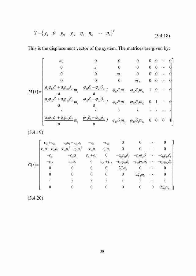
Then we get:

30

1 2 1 2

T

s t t nY y y y (3.4.18)

This is the displacement vector of the system. The matrices are given by:

1

2

2 11 1 1 21 2 11 1 21 211 1 1 21 2 2

2 12 1 1 22 2 12 1 22 212 1 1 22 2 2

2 1 1 1 2 2 1 1 2 21 1 1 2 2 2

0 0 0 0 0 0

0 0 0 0 0 0

0 0 0 0 0 0

0 0 0 0 0 0

1 0 0

0 1 0

0 0 0

s

t

t

s t t

s t t

n n n ns n t n t

m

J

m

m

a am J m mM t a a

a am J m m

a a

a am J m m

a a

1

(3.4.19)

1 2 1 1 2 2 1 22 2

1 1 2 2 1 1 2 2 1 1 2 2

1 1 1 1 1 1 11 1 1 12 1 1 1 1

2 2 2 2 2 2 21 2 2 22 2 2 2 2

1 1

2 2

0 0 0

0 0 0

0

0

0 0 0 0 2 0 0

0 0 0 0 0 2 0

0 0 0 0 0

s s s s s s

s s s s s s

s s s t t t t n

s s s t t t t n

c c c a c a c c

c a c a c a c a c a c a

c c a c c c c c

c c a c c c c cC t

0 0 2 n n

(3.4.20)

31

1 2 1 1 2 2 1 22 2

1 1 2 2 1 1 2 2 1 1 2 2

1 1 1 1 2

2 2 2 2 2

1 11 1 11 1 1 12 1 12 1 1 1 1 1 1

2 21 2

0

0

0 0 0 0

0 0 0 0

0 0 0 0

0 0 0

0 0 0

s s s s s s

s s s s s s

s s s s

s s s t

t t t t t n t n

t t

k k k a k a k k

k a k a k a k a k a k a

k k a k k

k k a k kK t

c k c k c k

c k

21 2 2 22 2 22 2 2 2 2 2 22

12

2

2

0 0

0 0

0 0

t t t n t n

n

c k c k

(3.4.21)

1 1 1 1 1

2 2 2 2 2

11 1 1 21 2 2

12 1 1 22 2 2

1 1 1 2 2 2

0

0

t t

t t

n n

c r k r

c r k rQ t

W W

W W

W W

(3.4.22)

Then according to the conditions we will write the functions for three time

ranges.

32

The first range: the vehicle runs on the bridge (that is to say the front wheel

is on the bridge) then 0

at

v

, so we can get 1 1 , 2 0

.

Then, the coefficients for the function of coupling system (3.4.17) will

become as follows:

1

2

211 11 11 1

212 12 12 1

21 1 1 1

0 0 0 0 0 0

0 0 0 0 0 0

0 0 0 0 0 0

0 0 0 0 0 0

10 1 0 0

10 0 1 0

10 0 0 0 1

s

t

t

s t

s t

s n n n t

m

J

m

m

am J mM t a a

am J m

a a

am J m

a a

(3.4.23)

1 2 1 1 2 2 1 22 2

1 1 2 2 1 1 2 2 1 1 2 2

1 1 1 1 1 1 11 1 12 1 1

2 2 2 2 2

1 1

2 2

0 0 0

0 0 0

0

0 0 0 0

0 0 0 0 2 0 0

0 0 0 0 0 2 0

0 0 0 0 0 0 0 2

s s s s s s

s s s s s s

s s s t t t t n

s s s t

n n

c c c a c a c c


c c a c c c c c

c c a c cC t

(3.4.24)

33

1 2 1 1 2 2 1 22 2

1 1 2 2 1 1 2 2 1 1 2 2

1 1 1 1 2 1 11 1 11 1 12 1 12 1 1 1 1

2 2 2 2 22

12

2

2

0 0 0

0 0 0

0

0 0 0 0

0 0 0 0 0 0

0 0 0 0 0 0

0 0 0 0 0 0

s s s s s s

s s s s s s

s s s s t t t t t n t n

s s s t

n

k k k a k a k k


k k a k k c k c k c k

k k a k kK t

(3.4.25)

1 1 1 1

11 1

12 1

1 1

0

0

0t t

n

c r k r

Q tW

W

W

(3.4.26)

The second range: the vehicle passed the bridge(that is to say that two

wheels on the bridge) then a l

tv v

, so we can get 1 2 1 .

Then, the coefficients for the function of coupled system (3.4.17) will

become as follows:

34

1

2

2 11 1 21 11 2111 1 21 2

2 12 1 22 12 2212 1 22 2

2 1 1 2 1 21 1 2 2

0 0 0 0 0 0

0 0 0 0 0 0

0 0 0 0 0 0

0 0 0 0 0 0

1 0 0

0 1 0

0 0 0 1

s

t

t

s t t

s t t

n n n ns n t n t

m

J

m

m

a am J m mM t a a

a am J m m

a a

a am J m m

a a

(3.4.27)

1 2 1 1 2 2 1 22 2

1 1 2 2 1 1 2 2 1 1 2 2

1 1 1 1 1 1 11 1 12 1 1

2 2 2 2 2 2 21 2 22 2 2

1 1

2 2

0 0 0

0 0 0

0

0

0 0 0 0 2 0 0

0 0 0 0 0 2 0

0 0 0 0 0 0 0 2

s s s s s s

s s s s s s

s s s t t t t n

s s s t t t t n

n n

c c c a c a c c


c c a c c c c c

c c a c c c c cC t

(3.4.28)

1 2 1 1 2 2 1 22 2

1 1 2 2 1 1 2 2 1 1 2 2

1 1 1 1 2 1 11 1 11 1 12 1 12 1 1 1 1

2 2 2 2 2 2 21 2 21 2 22 2 22 2 2 2 2

0 0 0

0 0 0

0

0

0

s s s s s s

s s s s s s

s s s s t t t t t n t n

s s s t t t t t t n t n

k k k a k a k k


k k a k k c k c k c k

k k a k k c k c k c kK t

2

12

2

2

0 0 0 0 0

0 0 0 0 0 0

0 0 0 0 0 0 n

(3.4.29)

35

1 1 1 1

2 2 2 2

11 1 21 2

12 1 22 2

1 1 2 2

0

0

t t

t t

n n

c r k r

c r k rQ t

W W

W W

W W

(3.4.30)

The third range: the vehicle get down the bridge(that is to say the back

wheel is still on the bridge) then l l a

tv v

, so we can get 1 0 ,

2 1 .

Then, the coefficients for the function of the coupled system (3.4.17) will

become as follows:

1

2

1 21 2121 2

1 22 2222 2

1 2 22 2

0 0 0 0 0 0

0 0 0 0 0 0

0 0 0 0 0 0

0 0 0 0 0 0

0 1 0 0

0 0 1 0

0 0 0 0 1

s

t

t

s t

s t

n ns n t

m

J

m

m

am J mM t a a

am J m

a a

am J m

a a

(3.4.31)

36

1 2 1 1 2 2 1 22 2

1 1 2 2 1 1 2 2 1 1 2 2

1 1 1 1 1

2 2 2 2 2 2 21 2 22 2 2

1 1

2 2

0 0 0

0 0 0

0 0 0 0

0

0 0 0 0 2 0 0

0 0 0 0 0 2 0

0 0 0 0 0 0 0 2

s s s s s s

s s s s s s

s s s t

s s s t t t t n

n n

c c c a c a c c


c c a c c

c c a c c c c cC t

(3.4.32)

1 2 1 1 2 2 1 22 2

1 1 2 2 1 1 2 2 1 1 2 2

1 1 1 1 2

2 2 2 2 2 2 21 2 21 2 22 2 22 2 2 2 22

12

2

2

0 0 0

0 0 0

0 0 0 0

0

0 0 0 0 0 0

0 0 0 0 0 0

0 0 0 0 0 0

s s s s s s

s s s s s s

s s s s

s s s t t t t t t n t n

n

k k k a k a k k


k k a k k

k k a k k c k c k c kK t

(3.4.33)

2 2 2 2

21 2

22 2

2 2

0

0

0

t t

n

c r k rQ t

W

W

W

(3.4.34)

37

4 MATLAB simulation

The governing equation for the coupled system was derived in chapter 3. In

this chapter, we will use MATLAB to numerically solve the equation based

on the Newmark-Beta method. A flow diagram for the MATLAB routine is

illustrated below.

39

Table 4.1 and Table 4.2 give the parameters used for the bridge and the

vehicle.

Table 4.1. Bridge parameters.[7]

Tab 4.2. Vehicle parameters.[7]

Item Data Item Data

/sm kg 38500 12 /tk N m 64.28 10

2/J kg m 62.446 10 11 /sc N sm 51.96 10

1 /tm kg 4330 12 /sc N sm 51.96 10

2 /tm kg 4330 11 /tc N sm 49.8 10

11 /sk N m 62.535 10 1

2 /tc N sm 49.8 10

12 /sk N m 62.535 10 1 /a m 4.2

11 /tk N m 64.28 10 2 /a m 4.2

1/v km h 40, 80, 120, 160

So we write the MATLAB code using the flow diagram and the parameters

The span

length

( )l m

The mass of bridge

per unit length

( / )kg m

The flexural rigidity

of the bridge 2( )EI N m

The damping

coefficient per unit

length

16 9360 102.05 10 0.025

40

given above. Simulation results are shown in the following chapters where

the influence of 1) vehicle speed, 2) bridge and 3) vehicle mass, is

demonstrated.

4.1 The influence of the speed

The simulated bridge displacement is shown in Fig. 4.1 to 4.2 for vehicle

speed 40 80, 120 and 160 km/h.

Figure 4.1 The mid-span dynamic displacement of bridge in different

speeds.

41

Figure 4.2 The vertical displacement of bridge at contact points for

different speeds (the upper figure is the first contact point, the lower figure

is second contact point).

From figure 4.1, we can get that the maximum of the mid-span

displacement will increase with the increasing speed of the vehicle,

although the relationship is not linear. We also can get that the maximum of

the mid-span displacement coming out is not when the vehicle runs on the

middle of the bridge. It happens on the left or right of the mid-span.

42

Figure 4.2 shows us that the maximum displacement of the bridge happens

when the vehicle locates in the front or back of the mid-span. With

increasing speed, the maximum displacement will increase. But, when the

speed is at some value, the value of the maximum displacement will be

smaller than that in the front speeds. This is related to the resonance of the

vehicle-bridge structures in combination with the speed of the vehicle.

The high frequency fluctuation is a result from the vehicle-bridge coupled

vibration. On the contrary, when the vehicle runs at high speed, the time for

the high frequency fluctuation is not enough to act sufficiently before the

vehicle gets down the bridge. Then the fluctuation of the curve will be

weak.

Fig 4.3 to 4.5 gives the displacement at the vehicle structure.

Figure 4.3 The vertical displacement of vehicle in different speeds.

43

Figure 4.4 The node angular displacement of vehicle in different speeds.

44

Figure 4.5 The vertical displacement of vehicle’s axle in different speeds

(the upper figure is for front axle, the lower figure is back axle).

4.2 The influence of the bridge’s span

The analysis is repeated with a longer bridge span using the parameters

shown below:

45

Table 4.3. Parameters of bridge. [8]

The span

length

( )l m

The mass of bridge

per unit length

( / )kg m

The flexural rigidity

of the bridge 2( )EI N m

The damping

coefficient per unit

length

50 32840 115.28 10 0.029

The result (for different speeds) can be seen in Fig. 4.6 to 4.10.


speeds.

46

Figure 4.7 The vertical displacement of bridge lie in contact point by


is for second contact point).

47



48


(the upper figure is front axle, the lower figure is for back axle).

By comparing figure 4.1 with figure 4.6, we can see that a bigger span leads

to a larger mid-span displacement of the bridge under the condition that the

vehicle runs at the same speed.

By comparing figure 4.4 with figure 4.9 we can get that as for the

small-span bridge especially when the length of the vehicle equals nearly

the length of the bridge, the node of the vehicle body has an obvious effect

49

on the response of the bridge.

4.3 The influence of mass of the vehicle

The difference when using a different set of parameters for the vehicle is

studied next.. The table below shows the new parameters.

Table 4.4. Parameters of vehicle.[8]

Item Data Item Data

/sm kg 15090 12 /tk N m 47.5 10

2/J kg m 53871 11 /sc N sm 41.2 10

1 /tm kg 190 12 /sc N sm 43.0 10

2 /tm kg 190 11 /tc N sm 600

11 /sk N m 53.7 10 1

2 /tc N sm 600

12 /sk N m 62.06 10 1 /a m 2.97

11 /tk N m 45.35 10 2 /a m 1.18

1/v km h 40, 80, 120, 160

We take the same span of 4.2 and run the MATLAB code. The result can be

seen in figure 4.11 to 4.15.

50


speeds.

51

Figure 4.12 The vertical displacement of bridge lie in contact point by


is for second contact point).

52



53


(the upper figure is for front axle, the lower figure is for back axle).

By comparing figure 4.11 with figure 4.6, we can get that the heavier mass

of the vehicle can make the fluctuation of the mid-span displacement of the

bridge more severe.

By comparing figure 4.12 with figure 4.7 we can get that the heavier the

mass of the vehicle is, the bigger the maximum displacement of the bridge

will be, under the condition that the vehicle runs at the same speed.

54

From figure 4.8 to 4.10 and figure 4.13 to 4.15, we can get that different

masses can affect the vehicle body vibrations significantly. As demonstrated

with these simulations, a vehicle running on a bridge with a heavy load can

lead to a strong dynamic interaction between the bridge and the vehicle

system.

4.4 Verification

A static calculation is carried out in order to verify the simulated

displacement.

We will verify the mid-span displacement of the bridge.

According to the Euler-Bernoulli beam theory and in the situation that the

point load is on the middle of the bridge we can get that:

24

4 Lx

EI

P

dx

d

(4.4.1)

Integrate it 4 times, we can get

13

3

2c

Lx

EI

P

dx

d

(4.4.2)

3221

2

2222

1cxcx

cLx

Lx

EI

P

dx

d

(4.4.3)

432231

3

26226

1cxcx

cx

cLx

Lx

EI

Px

(4.4.4)

And we also know that the boundary conditions are as follows:

55

0 0x

0x L

2

020xx

2

20x Lx

(4.4.5)

Then we can get that

3

4

4

10 0 0 (4.4.6)

6 2 2

0 sin 0 0

P L Lc

EI

c ce x if x

002

02

00 221

ccc

LL

EI

P (4.4.7)

EI

PcLc

LL

LL

EI

P

2220 11

1

(4.4.8)

LcLcL

LL

LEI

P3

31

1

3

6226

10

(4.4.9)

LcLEI

PL

EI

P3

33

12480

(4.4.10)

3

2

16c

EI

PL

(4.4.11)

So, we can get:

2262226

1

2 3

3

1

3L

cLcL

xLL

EI

PLx

(4.4.12)

EI

PL

EI

PLLx

32962

33

(4.4.13)

56

EI

PLLx

482

3

(4.4.14)

We take the “Table 4.1. Bridge parameters” and “Tab 4.2. Vehicle

parameters” as an example

These are parameters we will use:

1 2

10 2

m 38500

=m 4330

9.8 /

16

2.05 10 m

s

t t

kg

m kg

g N kg

L m

EI N

Substitute these parameters in the equation above we can get:

m0.00162

Lx

We then compare this static displacement with the simulated displacement

in figure 4.16.

57


speeds.

From this figure we can also find that when the vehicle runs to the centre of

the bridge the simulated displacement is around 0.0012 to 0.0015m. Hence,

it is verified that the simulated displacement produced by the model is

reasonable.

58

5 Conclusion and future work

5.1 Conclusion

In this work, we construct the models of the bridge and vehicle separately

based on the theory of vehicle-bridge coupled vibration. The models were

then connected by suing geometric relationships force equilibrium

conditions to construct the relation between the equation of the vehicle

vibration and the equation of bridge vibration. Finally, we use MATLAB to

handle the coupled problem based on the Newmark-β method. The

MATLAB code was then used to study the influence of various parameters.

As the simulation results show, the speed of the vehicle has a significant

effect on the dynamic response of the bridge. In general, the faster the

speed is, the bigger the maximum dynamic displacement is.

Also, when the span of the bridge is bigger, the maximum of displacement

will become bigger at the condition that the vehicle runs at the same speed.

When the mass of the vehicle increases, the maximum dynamic

displacement will increase significantly under the condition that the

vehicle’s speed is the same, and the span of the bridge is the same. And,

vehicles with different masses also affect the safety and comfort of the

drivers and passengers significantly.

5.2 Future work

5.2.1 Models and calculation method

In this thesis, we use two-dimensional models of the vehicle and bridge

system. The model and calculation method for the bridge is simplified to a

59

beam model , but for arch bridges with larger span and other bridges a

three-dimensional FEM-model could be more suitable . It is also possible to

extend the model of the vehicle. In this thesis, we take the two-axle lumped

vehicle model as an example to analyze the coupled vibration. A more

general FEM model could be considered for this purpose.

5.2.2 Numerical method

The Newmark-β method was used in this work to solve the governing

equations of motion. In this way, we lack the comparison between different

numerical methods. Other numerical methods, which are perhaps more

suitable for the studied problem, should be examined in future work.

60

6 References

[1] Wikipedia. (accessed October 2012). Euler–Bernoulli beam theory.

http://en.wikipedia.org/wiki/Euler%E2%80%93Bernoulli_beam_theory.

[2] Wikipedia. (accessed October 2012). D'Alembert's principle.

http://en.wikipedia.org/wiki/D'Alembert's_principle.

[3] Wikipedia. (accessed October 2012). Newmark-beta method.

http://en.wikipedia.org/wiki/Newmark-beta_method.

[4] WANG Hai-bo, CHEN Bo-wang, YU Zhi-wu. (2008). A Simplified

Numerical Integration Format of Newmark-β Method for Structural

Dynamic Equations. Journal of Sichuan University (Engineering Science

Edition), Vol.40 No.3, May 2008. Article ID: 1009-3087(2008)03-0047-06

[5] Clough, R.W.; Penzien, Joseph. (1993). Dynamics of Structures (2nd

Edition). ISBN-13: 978-0-07-011394-7.

[6] Xia He, Zhang Nan. (2002). Dynamic Interaction of Vehicles and

Structures. ISBN: 9787030100320

[7] XIAO Xin-biao, SHEN Huo-ming. (2004). Comparison of Three

Models for Vehicle-Bridge Coupled Vibration Analysis. Journal of

Southwest Jiaotong University. Vol.39 No.2 Apr. 2004. Article

ID:0258-2724(2004) 02-0172-04

[8] WANG Jiejun, ZHANG Wei,WU Weixiang. (2005). Analysis of

Dynamic Responses of Simply Supported Girder Bridge under Heavy

Moving Vehicles. Central South Highway Engineering. Vol.30 No.2

Jun,2005. Article ID: 1002-1205(2005)02-0055-03

61

Appendices

Appendix A: MATLAB scripts

main.m

clc

clear

close all

% the main program

global rou EI l mu

l=16;

mode=30; %input('how many mode shape ')

N=mode+4;

%parameters:

ms=38500;

mt1=4330;

mt2=4330;

J=2.446e6;

ks1=2.535e6;

ks2=2.535e6;

cs1=1.96e5;

cs2=1.96e5;

kt1=4.28e6;

kt2=4.28e6

ct1=9.8e4;

ct2=9.8e4;

a1=4.2;

a2=4.2;

62

a=a1+a2;

global rou EI l mu

rou=9360;

EI=2.05e10;

mu=0.025;

%%

velocity=40*1000/3600; % the speed of the car

T=(l+a)/velocity;

dt=0.000001*T;

t=0:dt:T;

t=t';

x=t*velocity;

level=1; %level:A=1,B=2.C=3......

nl=4;

NN=1000;

nu=5;

r=irregularity(level,NN,nl,nu,x); %level:A=1,B=2......

r_dot=(r(2:length(r))-r(1:length(r)-1))/dt;

A=zeros(N,length(t));

V=zeros(N,length(t));

X=zeros(N,length(t));

Q=zeros(N,length(t));

A0=zeros(N,1);

V0=zeros(N,1);

X0=zeros(N,1);

for jjj=1:length(t)

63

if t(jjj)*velocity<l;

delta1=1;

irr1=r(jjj);

irr_dot1=r_dot(jjj);

else delta1=0;

irr1=0;

irr_dot1=0;

end

if t(jjj)*velocity<l+a&t(jjj)*velocity>a;

delta2=1;

irr2=r(floor((t(jjj)*velocity-a)/dt/velocity)+1);

irr_dot2=r_dot(floor((t(jjj)*velocity-a)/dt/velocity)+1);

else delta2=0;

irr2=0;

irr_dot2=0;

end

[M,C,K]=MCK(ms,mt1,mt2,J,ks1,ks2,cs1,cs2,kt1,kt2,ct1,ct2,a1,a2,N,delta1,delta2,t(jjj),ve

locity);

Q=force(ct1,ct2,kt1,kt2,ms,a1,a2,mt1,mt2,irr1,irr2,irr_dot1,irr_dot2,velocity,t(jjj),delta1,de

lta2,N);

A0=M\(Q-C*V0-K*X0);

X1=X0+V0*dt+1/2*A0*dt^2;

V1=V0+A0*dt;

A1=M\(Q-C*V1-K*X1);

error1=1;

while error1>0.0001;

64

X2=X0+V0*dt+(1/2-1/4)*A0*dt^2+1/4*A1*dt^2;

V2=V0+(1-1/2)*A0*dt+1/2*A1*dt;

A2=M\(Q-C*V2-K*X2);

error1=sum(abs(abs(A2)-abs(A1)))/sum(abs(A1));

A1=A2;

V1=V2;

X1=X2;

end

X0=X1;

V0=V1;

A0=A1;

X(:,jjj)=X0;

V(:,jjj)=V0;

A(:,jjj)=A0;

end

save('D:\MATLABDATA\differentvelocity\A40','A');

save('D:\MATLABDATA\differentvelocity\V40','V');

save('D:\MATLABDATA\differentvelocity\X40','X');

save('D:\MATLABDATA\differentvelocity\Q40','Q');

MCK.m

function

[M,C,K]=MCK(ms,mt1,mt2,J,ks1,ks2,cs1,cs2,kt1,kt2,ct1,ct2,a1,a2,N,delta1,delta2,t,velocity)

%% N is the dimemsions of the matrix

global rou EI l mu

% rou is the constant like density ????

65

%% M matrix

M=zeros(N,N);

M1=[ms,J,mt1,mt2];

M1=diag(M1);

a=a1+a2;

for n=1:N-4

phi1n=sqrt(2/rou/l)*sin(n*pi*t*velocity/l);

phi2n=sqrt(2/rou/l)*sin(n*pi*(t*velocity-a)/l);

M(n+4,1)=(a1*phi1n*delta1+a2*phi2n*delta2)*ms/a;

M(n+4,2)=(phi1n*delta1-phi2n*delta2)*J/a;

M(n+4,3)=phi1n*delta1*mt1;

M(n+4,4)=phi2n*delta2*mt2;

end

M2=ones(N-4,1);

M2=diag(M2);

M(1:4,1:4)=M1;

M(5:N,5:N)=M2;

%% C matrix

C=zeros(N,N);

for n=1:N-4



C(3,n+4)=-ct1*phi1n*delta1;

C(4,n+4)=-ct2*phi2n*delta2;

end

C1=[cs1+cs2,cs1*a1-cs2*a2,-cs1,-cs2;...

cs1*a1-cs2*a2,cs1*a1^2+cs2*a2^2,-cs1*a1,cs2*a2;...

-cs1,-cs1*a1,cs1+ct1,0;...

66

-cs2,cs2*a2,0,cs2+ct2];

C2=mu/rou*diag(ones(N-4,1));

C(1:4,1:4)=C1;

C(5:N,5:N)=C2;

%% K matrix

K=zeros(N,N);

omega_n_2=zeros(1,N-4);

for n=1:N-4



phi1n_dot=n*pi/l*sqrt(2/rou/l)*cos(n*pi*t*velocity/l);

phi2n_dot=n*pi/l*sqrt(2/rou/l)*cos(n*pi*(t*velocity-a)/l);

K(3,n+4)=(-ct1*phi1n_dot-kt1*phi1n)*delta1;

K(4,n+4)=(-ct2*phi2n_dot-kt2*phi2n)*delta2;

omega_n_2(1,n)=EI/rou*(n*pi/l)^4;

end

K1=[ks1+ks2,ks1*a1-ks2*a2,-ks1,-ks2;...

ks1*a1-ks2*a2,ks1*a1^2+ks2*a2^2,-ks1*a1,ks2*a2;...

-ks1,-ks1*a1,ks1+kt1,0;...

-ks2,ks2*a2,0,ks2+kt2];

K2=diag(omega_n_2);

K(1:4,1:4)=K1;

K(5:N,5:N)=K2;

67

angulardisplacement.m

clc

clear

close all

l=16;

a1=4.2;

a2=4.2;

a=a1+a2;

rou=9360;


T=(l+a)/velocity;

dt=0.000001*T;

t=0:dt:T;

load('D:\MATLABDATA\differentvelocity\X40')

%% Change X V A for displacement, velocity and accelraction

[rows1,columns1]=size(X);

X_location=X(2,:);

rou=9360;

plot(t*velocity,X_location,'r-','LineWidth',1)

hold on

l=16;

a1=4.2;

a2=4.2;

a=a1+a2;

rou=9360;


T=(l+a)/velocity;

dt=0.000001*T;

68

t=0:dt:T;



X_location=X(2,:);

rou=9360;

plot(t*velocity,X_location,'b--','LineWidth',1)

hold on

l=16;

a1=4.2;

a2=4.2;

a=a1+a2;

rou=9360;


T=(l+a)/velocity;

dt=0.000001*T;

t=0:dt:T;



X_location=X(2,:);

rou=9360;

plot(t*velocity,X_location,'g-.','LineWidth',1)

hold on

l=16;

a1=4.2;

a2=4.2;

a=a1+a2;

rou=9360;


T=(l+a)/velocity;

dt=0.000001*T;

69

t=0:dt:T;



X_location=X(2,:);

rou=9360;

plot(t*velocity,X_location,'k:','LineWidth',1)

xlabel('The location of vehicle (m)')

ylabel('The node angular displacement of vehicle (m)')

title(' The node angular displacement of vehicle in different speeds')

legend('40km/h','80km/h','120km/h','160km/h','location','north')

axles.m

clc

clear

close all

l=16;

a1=4.2;

a2=4.2;

a=a1+a2;

rou=9360;


T=(l+a)/velocity;

dt=0.000001*T;

t=0:dt:T;




X_location=X(3,:);

rou=9360;

plot(t*velocity,X_location,'r-','LineWidth',1)

70

hold on

l=16;

a1=4.2;

a2=4.2;

a=a1+a2;

rou=9360;


T=(l+a)/velocity;

dt=0.000001*T;

t=0:dt:T;



X_location=X(3,:);

rou=9360;

plot(t*velocity,X_location,'b--','LineWidth',1)

hold on

l=16;

a1=4.2;

a2=4.2;

a=a1+a2;

rou=9360;


T=(l+a)/velocity;

dt=0.000001*T;

t=0:dt:T;



X_location=X(3,:);

rou=9360;

plot(t*velocity,X_location,'g-.','LineWidth',1)

71

hold on

l=16;

a1=4.2;

a2=4.2;

a=a1+a2;

rou=9360;


T=(l+a)/velocity;

dt=0.000001*T;

t=0:dt:T;



X_location=X(3,:);

rou=9360;

plot(t*velocity,X_location,'k:','LineWidth',1)

xlabel('The location of vehicle (m)')

ylabel('The vertical displacement of the front axle (m)')

title('The vertical displacement of axles in different speeds')


bridge_XVA.m

function X=bridge_XVA(modes,L,xG,mp)

%NM the mode shape % L the length of the bridge % xG the location

NM=length(modes);

X=zeros(size(xG));

for i=1:NM

X=X+sqrt(2/mp/L)*sin(i*pi*xG/L)*modes(i);

end

72

contactnew1.m

clc

clear

close all

l=50;

a1=2.97;

a2=1.18;

a=a1+a2;

rou=32840;


T=(l+a)/velocity;

dt=0.000001*T;

t=0:dt:T;

load('D:\MATLABDATA\differentvelocity3\X40')



X_location=zeros(columns1,1);

rou=32840;

X_contact1=zeros(length(t),1);


XXG1=zeros(length(t),1);


for jjj=1:length(t)


deltal1=1;

else deltal1=0;

end

73


deltal2=1;

else deltal2=0;

end

xG1=t(jjj)*velocity;

xG2=t(jjj)*velocity-a;

X_contact1(jjj)=bridge_XVA(X(5:rows1,jjj),l,xG1*deltal1,rou)*deltal1;


XXG1(jjj)=xG1;

XXG2(jjj)=xG2;

end

plot(XXG1,X_contact1,'r-','LineWidth',1)

hold on

l=50;

a1=2.97;

a2=1.18;

a=a1+a2;

rou=32840;


T=(l+a)/velocity;

dt=0.000001*T;

t=0:dt:T;




rou=32840;


74




for jjj=1:length(t)


deltal1=1;

else deltal1=0;

end


deltal2=1;

else deltal2=0;

end





XXG1(jjj)=xG1;

XXG2(jjj)=xG2;

end

plot(XXG1,X_contact1,'b--','LineWidth',1)

hold on

l=50;

a1=2.97;

a2=1.18;

a=a1+a2;

rou=32840;


T=(l+a)/velocity;

75

dt=0.000001*T;

t=0:dt:T;




rou=32840;





for jjj=1:length(t)


deltal1=1;

else deltal1=0;

end


deltal2=1;

else deltal2=0;

end





XXG1(jjj)=xG1;

XXG2(jjj)=xG2;

end

plot(XXG1,X_contact1,'g-.','LineWidth',1)

76

hold on

l=50;

a1=2.97;

a2=1.18;

a=a1+a2;

rou=32840;


T=(l+a)/velocity;

dt=0.000001*T;

t=0:dt:T;




rou=32840;





for jjj=1:length(t)


deltal1=1;

else deltal1=0;

end


deltal2=1;

else deltal2=0;

end



77



XXG1(jjj)=xG1;

XXG2(jjj)=xG2;

end

plot(XXG1,X_contact1,'k:','LineWidth',1)

xlabel('The location of the contact point (m)')

ylabel('The dynamic displacement of bridge on the first contact point (m)')

title('The dynamic displacement of bridge on the first contact point in different speeds')


contactnew2.m

clc

clear

close all

l=50;

a1=2.97;

a2=1.18;

a=a1+a2;

rou=32840;


T=(l+a)/velocity;

dt=0.000001*T;

t=0:dt:T;




78


rou=32840;





for jjj=1:length(t)


deltal1=1;

else deltal1=0;

end


deltal2=1;

else deltal2=0;

end





XXG1(jjj)=xG1;

XXG2(jjj)=xG2;

end

plot(XXG2,X_contact2,'r-','LineWidth',1)

hold on

l=50;

a1=2.97;

a2=1.18;

79

a=a1+a2;

rou=32840;


T=(l+a)/velocity;

dt=0.000001*T;

t=0:dt:T;




rou=32840;





for jjj=1:length(t)


deltal1=1;

else deltal1=0;

end


deltal2=1;

else deltal2=0;

end





XXG1(jjj)=xG1;

80

XXG2(jjj)=xG2;

end

plot(XXG2,X_contact2,'b--','LineWidth',1)

hold on

l=50;

a1=2.97;

a2=1.18;

a=a1+a2;

rou=32840;


T=(l+a)/velocity;

dt=0.000001*T;

t=0:dt:T;




rou=32840;





for jjj=1:length(t)


deltal1=1;

else deltal1=0;

end


81

deltal2=1;

else deltal2=0;

end





XXG1(jjj)=xG1;

XXG2(jjj)=xG2;

end

plot(XXG2,X_contact2,'g-.','LineWidth',1)

hold on

l=50;

a1=2.97;

a2=1.18;

a=a1+a2;

rou=32840;


T=(l+a)/velocity;

dt=0.000001*T;

t=0:dt:T;




rou=32840;




82


for jjj=1:length(t)


deltal1=1;

else deltal1=0;

end


deltal2=1;

else deltal2=0;

end





XXG1(jjj)=xG1;

XXG2(jjj)=xG2;

end

plot(XXG2,X_contact2,'k:','LineWidth',1)

xlabel('The location of the contact point (m)')

ylabel('The dynamic displacement of bridge on the second contact point (m)')

title('The dynamic displacement of bridge on the second contact point in different speeds')


force.m

function

Q=force(ct1,ct2,kt1,kt2,ms,a1,a2,mt1,mt2,r1,r2,r_dot1,r_dot2,velocity,t,delta1,delta2,N)

global rou l

a=a1+a2;

83

g=9.876;

W1=(ms*a2/a+mt1)*g;

W2=(ms*a1/a+mt2)*g;

Q=zeros(N,1);

Q(3)=(ct1*r_dot1+kt1*r1)*delta1;

Q(4)=(ct2*r_dot2+kt2*r2)*delta2;

for n=1:N-4;



Q(n+4)=-(phi1n*W1*delta1+phi2n*W2*delta2);

end

irregularity.m

function r=irregularity(level,N,nl,nu,x)

Gdn0=4^(level+1)*10^(-6);

detal_n=(nu-nl)/N;

n0=0.1;

r=zeros(length(x),1);

W=2;

for k=1:N

nk=nl+(k-0.5)*detal_n;

Gdn=Gdn0*(nk/n0)^(-W);

Ank=sqrt(4*Gdn*detal_n);

r=r+Ank*cos(2*pi*nk*x+rand(1)*2*pi);

end

School of Engineering, Department of Mechanical Engineering Blekinge Institute of Technology SE-371 79 Karlskrona, SWEDEN

Telephone: E-mail:

+46 455-38 50 00 [email protected]

modelling and simulation of a bridge interacting with a moving …829478/fulltext01.pdf · the...

Documents