modelling and optimisation of flexib le pvc compound

CVD800 2016-11-24

Modelling and Optimisation of Flexible PVC Compound

Formulation for Mine Cables

Fechter, RH

© University of Pretoria

CVD800 2016-11-24



Fechter, RH

11010152

Department of Chemical Engineering

University of Pretoria


ii



Synopsis

The thermal stability, fire retardancy and basic mechanical properties, as a

function of the mass fractions of the poly(vinyl chloride) (PVC) compound

ingredients, can be modelled using 2nd order Scheffé polynomials. The empirical

models for each response variable can be determined using statistical

experimental design. The particular models for each response variable, which are

selected for predictive ability using k-fold cross validation, can be interpreted

using statistical analysis of the model terms. The statistical analysis of the model

terms can reveal the synergistic or antagonistic interactions between ingredients,

some of which have not been reported in literature. The interaction terms in the

models also mean that the effect of a certain ingredient is dependent on the mass

fractions of the other ingredients. Sensitivity analysis can be used to examine the

overall effect of a change in a particular formulation on the response variables.

The empirical models can be used to minimise the cost of the PVC compound by

varying the formulation. The optimum formulation is a function of the costs of the

various ingredients and the limits which are placed on the response variables. To

analyse the system as a whole, parametric analysis can be used. The number of

different parametric analyses which can be done is very large and depends on the

specific questions which need to be answered. Parametric analysis can be used to

gain insight into the complex behaviour of the system with changing requirements,

as a decision making tool in a commercial environment or to determine the

completeness of the different measuring techniques used to describe the thermal

stability and fire retardancy of the PVC compound. Statistical experimental design

allows for the above methods to be used which leads to significant time and labour


iii

savings over attempting to reach the same conclusions using the traditional one-

factor-at-a-time experiments with changes in the phr of an ingredient.

It is recommended that the data generated for this investigation is analysed in

more detail using the methods outlined for this investigation. This can be

facilitated by making the analysis of the data (and therefore the data itself) more

accessible through a usable interface. The data set itself can also be expanded to

include new ingredients requiring very few additional experiments. If a PVC

compound that contains none of the ingredients that were used in this

investigation is of interest a new separate data set needs to be generated. This can

be done by following the same procedure used in this investigation. In fact the

method that is used in this investigation can be generalised to optimise the

proportions of the ingredients of any mixture.

Keywords: PVC, mine cables, statistical experimental design, mixture optimisation


iv

Acknowledgements

• My supervisors, Dr. Johan Labuschagne and Carl Sandrock

• Dr. Ines Kühnert, Dr. Andreas Leuteritz, Martin Zimmermann, Andreas

Scholze and Yvonne Spörer of the Leibniz-Institut für Polymerforschung

Dresden e.V.

• Harry Wright, Gerard James, Chirlene Botha and Isbe van der Westhuizen of

the Institute of Applied Materials at the University of Pretoria

• Dr. Manfred Scriba and Gertrude Makgatho of the CSIR

• National Research Foundation of South Africa

• University of Pretoria StudyAbroad Bursary Programme


v

Contents

Synopsis...............................................................................................................................................................................ii

Acknowledgements .................................................................................................................................................. iv

Contents............................................................................................................................................................................... v

Nomenclature............................................................................................................................................................. viii

1 Introduction.......................................................................................................................................................... 1

2 Theory ....................................................................................................................................................................... 3

2.1 PVC ....................................................................................................................................................................... 3

2.1.1 Additives ................................................................................................................................................ 4

2.1.1.1 Thermal Stabilisers.............................................................................................................. 4

2.1.1.2 Plasticisers.................................................................................................................................. 5

2.1.1.3 Fire Retardants ....................................................................................................................... 6

2.1.1.4 Fillers .............................................................................................................................................. 7

2.1.2 Applications ........................................................................................................................................ 8

2.1.2.1 Cables for Underground Mines .................................................................................. 9

2.1.3 Processing.......................................................................................................................................... 10

2.1.3.1 Compounding ........................................................................................................................ 10

2.1.3.2 Final Part Fabrication ..................................................................................................... 12

2.1.4 Testing Methods ........................................................................................................................... 12

2.1.4.1 Thermal Stability ................................................................................................................ 12

2.1.4.2 Fire Retardancy ................................................................................................................... 17

2.1.4.3 Mechanical Properties ................................................................................................... 21

2.1.5 Environmental Concerns ....................................................................................................... 23

2.1.6 Comments on the Economics of PVC............................................................................ 24

2.2 Layered Double Hydroxides ......................................................................................................... 24

2.3 Fly Ash as a Spherical Filler........................................................................................................... 25

2.4 Statistical Design of Experiments ............................................................................................. 26


vi

2.4.1 Mixtures .............................................................................................................................................. 27

2.5 Model Selection and K-fold Cross-Validation.................................................................. 31

3 Optimisation ...................................................................................................................................................... 33

3.1 Problem Statement .............................................................................................................................. 33

3.2 Definition of Design Variables..................................................................................................... 33

3.3 Identification of the Objective Function.............................................................................. 34

3.4 Identification of Constraints ......................................................................................................... 35

4 Experimental Design................................................................................................................................... 37

4.1 Selection of the Response Variables....................................................................................... 37

4.2 Choice of Factors and Ranges ...................................................................................................... 38

4.3 Choice of Experimental Design................................................................................................... 43

4.4 Performing the Experiments ........................................................................................................ 44

4.4.1 Compound Preparation .......................................................................................................... 44

4.4.2 Torque Rheometer...................................................................................................................... 46

4.4.3 Thermomat ....................................................................................................................................... 47

4.4.4 Colour.................................................................................................................................................... 48

4.4.5 Cone Calorimetry ......................................................................................................................... 49

4.4.6 MCC ......................................................................................................................................................... 49

4.4.7 LOI............................................................................................................................................................ 50

4.4.8 Tensile Test ...................................................................................................................................... 50

5 Results and Discussion.............................................................................................................................. 52

5.1 Model Selection ....................................................................................................................................... 52

5.2 Model Analysis......................................................................................................................................... 57

5.2.1 Statistical Significance of Model Terms ..................................................................... 57

5.2.2 Sensitivity Analysis .................................................................................................................... 60

5.3 Optimisation .............................................................................................................................................. 67

5.3.1 Optimum Solution ....................................................................................................................... 67

5.3.2 Parametric Analysis ................................................................................................................... 72


vii

5.3.2.1 Change in Response Variable Constraint Value ......................................... 72

5.3.2.2 Change in Cost of Ingredient ..................................................................................... 76

5.3.2.3 Change in Response Variables Constrained.................................................. 79

5.4 Implementation ...................................................................................................................................... 81

5.5 Labour and Time Savings................................................................................................................ 81

6 Conclusions and Recommendations .............................................................................................. 85

6.1 Response Variable Models ............................................................................................................. 85

6.2 Optimisation .............................................................................................................................................. 87

7 Future Work ...................................................................................................................................................... 90

8 References........................................................................................................................................................... 93


viii

Nomenclature

c Cost of ingredient R/kg

D Design variables matrix

E Elastic Modulus MPa

f Objective function value R/kg

k Number of folds for k-fold cross-validation

m Empirical conductivity model slope μS/(cm·min)

n Degree of Scheffé polynomial

N Number of terms

Ne Number of experimental points

p Material property value

plim Limit on material property value

q Number of components

t Time min

Tg Glass transition temperature °C

tint Time at intercept min

vT Cross-head speed mm/min

X CIE tristimulus value

x Mass fraction

X Transformed design variable matrix

xDINP Mass fraction of DINP

xfill Mass fraction of filler

xFR Mass fraction of FR

xLDH Mass fraction of LDH

xPVC Mass fraction of PVC

xsph.fill Mass fraction of spherical filler

xstab Mass fraction of primary stabiliser

Y CIE tristimulus value

y Response variable value


ix

y Response variable value vector

y* Scaled response variable value

YI Yellowing Index

ymax Minimum response variable value

ymin Maximum response variable value

Z CIE tristimulus value

Greek

β Empirical conductivity model constant μS/cm

β Model parameters vector

𝛃𝛃� Estimated model parameter vector

βi Scheffé polynomial linear parameter

βij Scheffé polynomial two-way interaction parameter

βijk Scheffé polynomial three-way interaction parameter

γij Scheffé polynomial antisymmetric two-way

interaction parameter

ϵ Measurement error vector

θ Empirical conductivity model constant

σ Conductivity μS/cm

σmin Conductivity offset μS/cm

τ Empirical conductivity model constant min


1

1 Introduction

PVC is a commercially significant thermoplastic. With the use of a large variety of

additives the properties of PVC can be modified and tailored to a specific

application making it a very versatile plastic. One of the many types of additives

used for PVC are Layered Double Hydroxides (LDHs). LDHs are used as thermal

stabilisers and fire retardants in PVC. Developments by Labuschagne et al. (2006)

in the manufacture of LDHs have led to a patent describing a new effluent free

synthesis method. To make the LDHs produced using the new synthesis method

commercially viable requires that they have product applications. One such

application is as an additive for flexible PVC compound used for the insulation

material for cables used in South African underground mines.

However this means that a new formulation is required that incorporates the LDH.

The problem is that a PVC compound is a complex system where there are many

interactions between the different additives. The problem is further complicated

by the fact that the additives tend to have an effect on multiple properties of the

PVC compound, and that the PVC compound is essentially a mixture system which

means that changes in the proportion of a certain ingredient are not independent.

Traditionally PVC formulations are developed over many years by experienced

PVC formulators using a predominantly best-guess trial and error approach.

Although this has been used very successfully in the past it is not very flexible

when it comes to introducing new additives. The traditional approach is also

focused more on finding acceptable rather than optimum formulations.

The purpose of the investigation is to develop a method that can be used to find an

optimum flexible PVC formulation for the insulation used for underground mine

cables by varying the proportions of the ingredients included in the PVC

compound. It is also required that the method facilitates the analysis of the effects

and interactions of the various ingredients that are used.


2

A Ca-Al LDH manufactured using the effluent free method, a spherical fly ash filler

and the industry standard primary thermal stabiliser, plasticiser, fire retardant

filler and PVC resin are used. The thermal stability, fire retardancy and basic

mechanical properties of the PVC compound are modelled as a function of the mass

fractions of the ingredients using statistical experimental design. The resultant

empirical models are used to demonstrate how the system can be optimised and

consequently analysed using a parametric analysis. The experimental design is

done using JMP Statistical Software, the experiments are conducted in a laboratory

environment and the data analysis is done using programmes written in Python

programming language.


3

2 Theory

2.1 PVC

PVC is a commercially important and versatile thermoplastic which is synthesised

using free-radical polymerisation of the vinyl chloride monomer (Wilkes, et al.,

2005). PVC is the third most produced polymer in the world after polyethylene

(PE) and polypropylene (PP). In 2013 the estimated global consumption of PVC

was 39.3 million tonnes (Ceresana Research, 2014). Since the commercialisation

of PVC in the 1930s the PVC industry has grown in spite of a number of challenges

such as developing non-toxic thermal stabilisers and plasticisers (Braun, 2004).

This pattern of increasing growth is still relevant with a predicted increase of 3.2%

per year in the global demand for PVC (Ceresana Research, 2014).

Many of the interesting and unique aspects of PVC are due to the fact that it

contains chlorine. The chemical structure of PVC is shown in Figure 1.

Figure 1: Chemical Structure of PVC (Wilkes, et al., 2005)

The chlorine content of PVC by mass is approximately 58 %, meaning that PVC

requires significantly less natural gas and oil as a raw material than other major

polymers such as PP and PE, which are completely hydrocarbon based (Wilkes, et

al., 2005). PVC is also an important chlorine sink. Chlorine is produced primarily

as a by-product of the production of sodium hydroxide which is used in many

industries as a strong base (Braun, 2004). In terms of the material properties the


4

presence of the chlorine atom makes PVC moderately polar and inherently flame

retardant (Wilkes, et al., 2005).

2.1.1 Additives

The polarity of PVC combined with its amorphous structure make it compatible

with a large number of different additives (Braun, 2004). The additives perform

essential functions during processing of the PVC and influence the properties of

the final product (Wypych, 2009).

2.1.1.1 Thermal Stabilisers

The presence of the chlorine in PVC, although helpful in many aspects, also results

in an autocatalytic thermal degradation reaction. The degradation reaction is

initiated by the release of labile chlorine from unstable chlorine groups such as

allylic and tertiary chlorides which are a result of structural irregularities in the

polymer (Wilkes, et al., 2005) (Schiller, 2015). During the thermal degradation

hydrogen chloride (HCl) is released and double bonds are formed. The HCl acts as

a catalyst for the degradation reaction (Bacaloglu & Fish, 1995). The thermal

degradation reaction for neat PVC occurs below typical processing temperatures

of 170 °C to 220 °C making it impossible to process PVC without the use of thermal

stabilisers (Gupta, et al., 2009).

Stabilisers are grouped in two basic categories: primary and secondary stabilisers.

Primary stabilisers react with the allylic chlorides preventing the initiation of the

degradation reaction. Due to the autocatalytic nature of the degradation, once the

process is initiated it accelerates very quickly. The primary stabilisers are essential

for the inhibition of the initial step to maintain early stability. A number of primary

stabilisers are available commercially including mixed metal stabilisers and

organotins (Bacaloglu & Fisch, 2000).


5

Secondary stabilisers are substances which have the ability to scavenge HCl. The

removal of HCl cannot prevent the initial degradation step but inhibits the

abovementioned auto-catalytic degradation. This means that a secondary

stabiliser used in isolation cannot give short term stability, but provides good long

term stability (Bacaloglu & Fisch, 2000). LDHs and Zeolites are two materials

commonly used as secondary stabilisers (Gupta, et al., 2009).

To obtain PVC with short and long term stability primary and secondary stabilisers

are often combined (Bacaloglu & Fisch, 2000). The choice and amount of additives

used together to form a so called ‘stabilisation package’ is important due to the fact

that synergistic and antagonistic interactions between different stabilisers are

common (Schiller, 2015).

2.1.1.2 Plasticisers

Plasticisers are substances that are incorporated into PVC to increase its flexibility

and workability. The general plasticiser for PVC must contain a polar and non-

polar chemical group. The polar part of the plasticiser molecule is able to bind with

the polar PVC molecule while the non-polar part of the molecule limits the

interaction of the PVC molecules with each other through van der Waal’s forces.

The non-polar part of the molecule also creates additional free volume and

provides some lubrication. All of these mechanisms contribute to the plasticisation

of the PVC (Wilkes, et al., 2005).

The most commonly used chemicals for the plasticisation of PVC are phthalate

esters, constituting approximately 87% of all PVC plasticisers (Schiller, 2015). The

polar carbon-chloride bond (Cδ+ - Clδ-) in PVC is particularly attracted to the

carbonyl bond (Cδ+ = Oδ-) in esters while the aliphatic side chain of the ester is the

non-polar part of the molecule (Wilkes, et al., 2005). Traditionally diethylhexyl


6

phthalate (DEHP or DOP) was the most commonly used phthalate but it has been

mostly replaced by diisononyl phthalate (DINP) (Schiller, 2015).

Plasticisers have a significant effect on both the processing of PVC and the final

PVC part. During processing the plasticiser reduces internal friction and adhesion

to metal surfaces (which can be a problem due to the polarity of PVC) through its

lubricating effect while also decreasing the required processing temperature. In

the final part the plasticiser reduces the elastic modulus E, tensile strength and

glass transition temperature while increasing the elongation at break, bending

strength and antistatic properties. The easy incorporation of plasticisers into PVC

result in a broad range of compounds with different flexibilities from rigid PVC

with no plasticiser to highly flexible PVC compounds that can be tailored to specific

and varying applications (Schiller, 2015). A distinct disadvantage of using

plasticisers, which are generally used in significant quantities in flexible PVC

formulations, is that (with the exception of phosphoric acid esters) plasticisers are

highly flammable (Wypych, 2009).

2.1.1.3 Fire Retardants

PVC is inherently fire and flame retardant. The high chlorine content means that

there is less fuel available for combustion in contrast to completely hydrocarbon-

based polymers such as PE which burn readily. The chlorine in the PVC also

removes hydrogen as a fuel source from the condensed phase, through a radical

trapping mechanism, producing HCl (in addition to the HCl produced through

thermal degradation). The HCl in turn dilutes the gas phase decreasing the oxygen

concentration (Wilkes, et al., 2005). The final fire retarding mechanism that is

inherent to PVC is the formation of a char. Char formation is a desirable property

for fire retardancy because the char acts as a barrier to heat and to the release of

volatiles, which decreases the fuel available to the flame. Char formation also

decreases smoke production (Wypych, 2008). Due to this inherent fire retardancy


7

rigid PVC does not require fire retarding additives. In flexible PVC compounds,

however, fire retardants are required due to the flammability of the plasticisers as

discussed in Section 2.1.1.2 (Wypych, 2009).

The main fire retardant used for flexible PVC is antimony trioxide (Sb2O3). During

combustion Sb2O3 forms antimony trichloride (SbCl3) which acts as a flame

inhibitor by trapping radicals in a similar mechanism to the PVC itself (Levchik &

Weil, 2005). Sb2O3 is generally added to PVC in relatively low concentrations. The

other flame retardant additive used frequently in PVC is aluminium trihydrate

(ATH). In contrast to Sb2O3 relatively high concentrations of ATH are required to

have a reasonable effect on the flame retardancy (Wypych, 2009). Fortunately

ATH is relatively cheap and so is used effectively as a functional filler. ATH and

other mineral fire retardant fillers (such as magnesium hydroxide (Mg(OH)2)

which is also used in PVC) work through two different mechanisms. The first is

through the release of water during combustion which dilutes the combustible

pyrolysis products in the gas phase. The second is by providing a substantial

inorganic residue which promotes the formation of a char and provides a barrier

to heat and mass transfer (Levchik & Weil, 2005).

2.1.1.4 Fillers

Fillers are the most abundantly used additives by mass in PVC and other polymers.

The main purpose of fillers is to reduce the overall material cost of a polymer

compound (Wypych, 2009). The most commonly used filler in all polymers

including PVC is calcium carbonate (CaCO3). The main advantages of CaCO3, which

make it popular as a mineral filler, are its low cost, low hardness, wide range of

possible particle size distributions, its low refractive index and high whiteness

(Wilkes, et al., 2005). The main disadvantage of using CaCO3 is that it contains no

chemical groups in its structure which interact, through van der Waals forces, with

the PVC matrix. This results in a decrease in the mechanical performance of the


8

compound and makes it more difficult to process. A common way to decrease the

adverse effects of CaCO3 and other mineral fillers is to surface treat them with a

compatibiliser. The CaCO3 also has a low packing density which means that for

flexible PVC compounds more plasticiser is required (Wypych, 2009).

2.1.2 Applications

PVC is the most versatile plastic currently known. Its versatility is primarily as a

result of its polarity which makes plasticisation possible (discussed in section

2.1.1.2). PVC applications vary from rigid construction products such as pipes,

sidings and window profiles to semi-rigid flooring and wall coverings to flexible

products such as medical tubing and cable insulation (Wilkes, et al., 2005). The

broad range of applications is also a consequence of the large variety of other

additives that can be incorporated into PVC (discussed in section 2.1.1) and some

of PVC’s unique properties. These properties include its resistance to

environmental attack, particularly against exposure to hydrocarbons, and its

tendency to crosslink rather than undergo chain scission during degradation from

oxidation or UV exposure. These properties make it particularly suited to

applications with a long service life. The main applications as a percentage of PVC

production in Europe in 2014 are shown in Figure 2 (European Council for Vinyl

Manufacturers, 2014).


9

Figure 2: PVC applications as a percentage of PVC production in the EU in 2014

(European Council for Vinyl Manufacturers, 2014)

2.1.2.1 Cables for Underground Mines

One application where PVC is used is for the sheathing (also referred to as

jacketing) and insulation of low voltage power cables in underground mines.

Cables in underground mines need to be flexible, protected from mechanical

damage, fire resistant, corrosion resistant and resistant against oils and other

hydrocarbons. The fire retardancy requirements are particularly stringent due to

the confined spaces found in mines (Khastgir, 2009).

Cable jackets are primarily made from four different types of materials:

• Fibrous materials

• Rubber and rubber-like materials

• Metallic materials

0

5

10

15

20

25

30PV

C Us

ed (

%)


10

• Thermoplastics

Thermoplastic jackets have some fundamental physical and financial advantages

over the other more traditional jackets (Shoemaker & Mack, 2012). The two

thermoplastics used most commonly are PVC and PE (Shoemaker & Mack, 2012)

(Pabla, 2011) (Joshi, 2008).

In general PVC is well suited as an insulating and protective sheath material for

wires and cables due to its good dielectric strength, fire retardancy, low weight

and durability. The versatility of PVC compound means that it can be tailored to

the specific operating conditions of many wire and cable applications by changing

the formulation (Wilkes, et al., 2005).

2.1.3 Processing

2.1.3.1 Compounding

In almost all polymer processes the quality of the final part is influenced by the

quality of the mixing of all the different constituents of the polymer compound. In

polymer science there are two defined forms of mixing namely distributive and

dispersive mixing (Osswald, 2010). The aim of distributive mixing is to improve

the spatial distribution of the ingredients without overcoming the cohesive forces

to break down agglomerates. Dispersive mixing has to overcome cohesive forces

so that it can break down agglomerates into their primary particle sizes.

Dispersive mixing is effectively a more rigorous and finer version of distributive

mixing (Murphy, 2001).

Due to some of the unique features of PVC and the various additives that are used,

the compounding of PVC is generally performed in two steps; a powder mixing

step that is predominantly distributive followed by a dispersive compounding


11

step. The powder mixing step is done for a number of reasons. The first is to

disperse the different particulate additives and the PVC resin powder. The second

is to heat the PVC resin to a temperature above its glass-transition temperature

(Tg = 82 °C) so that the plasticiser (which is typically a liquid) is rapidly absorbed

by the PVC resin particles. This is achieved using a high speed shear mixer. For

high speed mixing the dry PVC resin powder, particulate additives and liquid

plasticiser are added to the mixer. At room temperature the diffusion rate of the

plasticiser into the PVC is very low so that initially, during mixing, a wet, caked

powder is formed. The temperature of the caked powder increases as the mixing

progresses due to the friction that is generated. As the temperature of the powder

increases the diffusion rate of the plasticiser into the PVC increases. When the

temperature rises to just above Tg the plasticiser is rapidly absorbed and a dry

powder is formed. It is important that the mixing time is only as long as it takes for

all the plasticiser to be absorbed. If mixing continues after a dry powder has been

formed the temperature of the powder will continue to rise and the PVC may

undergo thermal degradation. It is also important to note that there is an upper

limit to the amount of plasticiser that can be absorbed by the PVC (depending on

the grade of PVC). If high speed mixing was done correctly a well distributed dry

powder is formed (Wilkes, et al., 2005).

The next step is to disperse the agglomerated additives throughout the PVC matrix.

The PVC itself also needs to be dispersed due to the fact that it exists as

agglomerates of smaller primary PVC particles in its powdered form. The

dispersion is achieved through melting the PVC and applying elongational (as

opposed to shear) work to the PVC melt. This second compounding step can be

done in the same step as forming the final part or as a separate compounding step.

Compounding equipment used for this step includes batch internal mixers

(Banbury), continuous internal mixers, single screw compounders, reciprocating

single screw compounders (Buss Kneader) and co- and counter-rotating twin

screw compounders (Wilkes, et al., 2005).


12

2.1.3.2 Final Part Fabrication

As mentioned, processing of PVC is not possible without additives. However, the

formulation of PVC compounds can be manipulated to enable a number of different

processing methods for final part fabrication. The main processing methods in use

are blow moulding, calendaring, sheet extrusion, profile extrusion, wire and cable

extrusion, thermoforming and injection moulding (Wilkes, et al., 2005).

The main difficulty with processing PVC is its inherent thermal instability and the

autocatalytic nature of the thermal degradation process. The rapid nature in which

the degradation reaction can occur, once initiated, and the resulting crosslinking

of the polymer chains can lead to catastrophic failure during processing. This,

however, can be avoided by sufficiently stabilising the PVC compound and

designing PVC processing equipment accordingly. General processing practices

which lower the risk of PVC degrading during processing, to a point where the final

part is compromised, include: decreasing residence time and avoiding stagnation

zones where PVC compound can accumulate and initiate degradation (Wilkes, et

al., 2005).

2.1.4 Testing Methods

2.1.4.1 Thermal Stability

Determining the thermal stability of a PVC compound is a crucial part of evaluating

its suitability for processing. A number of methods to test the thermal stability of

PVC compounds have been developed over the years using different mechanisms

and principles of the degradation process. The methods can be broadly classified

into those that measure static thermal stability and those that measure dynamic

stability. The main methods used to determine the thermal stability of PVC are


13

torque rheometer testing (dynamic), HCl evolution testing (generally static) and

oven stability testing (static) (Wilkes, et al., 2005) (Wypych, 2008).

2.1.4.1.1 Torque Rheometer

The torque rheometer is the single best piece of laboratory equipment to measure

the dynamic thermal stability of PVC (Wilkes, et al., 2005). A torque rheometer is

essentially a batch mixer where the torque applied to the rotors, at constant

rotational speed, and the temperature of the polymer melt as a function of time are

measured (Ari, 2010). A schematic diagram of the mixing chamber of a torque

rheometer is shown in Figure 3

Figure 3: Mixing chamber of a torque rheometer (Wilkes, et al., 2005)

To determine the dynamic thermal stability of a PVC compound, the compound is

introduced into the mixing chamber which is heated to a set temperature. After

the initial melting of the PVC the torque measurement will stabilise at a certain

resting torque until the PVC starts to degrade thermally. The thermal degradation

causes crosslinking of the polymer chains which leads to an increase in the torque

required to maintain the rotational speed of the rotors. The thermal stability time

is defined as the time from when the PVC has melted to the point where thermal


14

degradation has started (Wilkes, et al., 2005). A typical torque curve is shown in

Figure 4.

Figure 4: Typical torque curve measured using a torque rheometer for a flexible

grade PVC (ASTM, 2002)

Besides giving information about the dynamic thermal stability of a PVC

compound, the torque curve also gives information on the viscosity and general

flow behaviour of the PVC. The combination of all this information makes the

torque rheometer an excellent instrument for gaining insight into the processing

behaviour of PVC compounds (Ari, 2010).

2.1.4.1.2 Thermomat

A Thermomat (also called a Rancimat) is used to measure the evolution of HCl from

PVC as it is heated isothermally. The HCl released during heating is a product of

the thermal degradation reaction (as discussed in section 2.1.1.1.). Therefore, a

measurement of the HCl evolution is effectively a measurement of the thermal

degradation of the PVC compound. A Thermomat works by isothermally heating a

small amount of PVC in a sample holder. The gases that evolve from the PVC are

swept to a separate container, holding distilled water, with nitrogen. The


15

conductivity of the water is measured as a function of time. The conductivity and

the HCl content are directly proportional (Wypych, 2008).

As is the case with the torque curve produced by the torque rheometer, some work

is required to obtain a quantitative measure of the thermal stability (in this case

static thermal stability) from the conductivity curve. A simple method to obtain a

thermal stability time from the conductivity curve is to define a conductivity value

such that the stability time is the time it takes the conductivity to exceed the

defined value. Figure 5 demonstrates this principle for conductivity curves from

an investigation into the stabilisation of PVC with LDHs (Labuschagne, et al., 2015)

Figure 5: Conductivity curves for PVC stabilised with different LDHs

(Labuschagne, et al., 2006)

It is clear from Figure 5 that the abovementioned method is flawed due to the fact

that the stability time is effectively based on a single data point where the

threshold conductivity is exceeded. A method is required that uses all of the

available data points to determine the stability time so that the global shape of the

conductivity curve is taken into account. This can be achieved by fitting the

following model to the conductivity curve


16

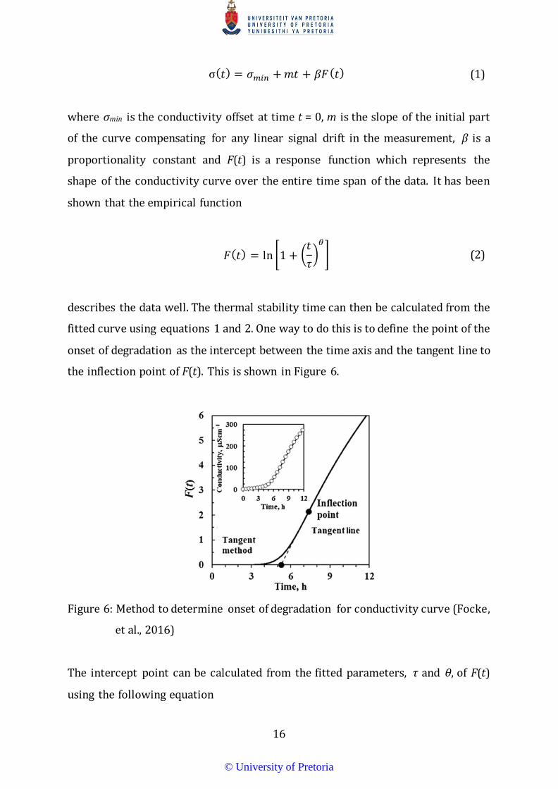
σ(𝑡𝑡) = 𝜎𝜎𝑚𝑚𝑚𝑚𝑚𝑚 +𝑚𝑚𝑡𝑡 + 𝛽𝛽𝛽𝛽(𝑡𝑡) (1)

where σmin is the conductivity offset at time t = 0, m is the slope of the initial part

of the curve compensating for any linear signal drift in the measurement, β is a

proportionality constant and F(t) is a response function which represents the

shape of the conductivity curve over the entire time span of the data. It has been

shown that the empirical function

𝛽𝛽(𝑡𝑡) = ln �1 + �𝑡𝑡𝜏𝜏�𝜃𝜃� (2)

describes the data well. The thermal stability time can then be calculated from the

fitted curve using equations 1 and 2. One way to do this is to define the point of the

onset of degradation as the intercept between the time axis and the tangent line to

the inflection point of F(t). This is shown in Figure 6.

Figure 6: Method to determine onset of degradation for conductivity curve (Focke,

et al., 2016)

The intercept point can be calculated from the fitted parameters, τ and θ, of F(t)

using the following equation


17

𝑡𝑡𝑚𝑚𝑚𝑚𝑖𝑖 = 𝜏𝜏(𝜃𝜃 − 1)1𝜃𝜃 �1−

ln(𝜃𝜃)(𝜃𝜃 − 1)� (3)

The time taken to reach the onset of degradation (which is effectively tint) is then

defined as the thermal stability (Focke, et al., 2016).

2.1.4.1.3 Colour

It is well documented that during thermal degradation the colour of PVC changes.

This has been linked with the number and length of polyene sequences formed in

the PVC matrix as a result of the degradation reaction (Wilkes, et al., 2005). The

colour stability of PVC is typically measured using different oven aging techniques.

Traditionally the colour of different samples was visually inspected using

reference samples. A more modern method uses scans or images of the PVC

samples. The colour of the image or scan is captured numerically using the CIE

tristimulus values. The CIE tristimulus values are then expressed as a yellowing

index (YI) using the following equation.

𝑌𝑌𝑌𝑌 = 1001.28𝑋𝑋 − 1.06𝑍𝑍

𝑌𝑌 (4)

where X, Y and Z are the CIE tristimulus values. Generally, as the PVC becomes

more degraded YI will increase. This technique allows for a more scientific and

repeatable comparison of the colours of different PVC samples (Wypych, 2008).

2.1.4.2 Fire Retardancy

Testing the fire retardancy of materials is difficult due to the complexity and poor

reproducibility of fires. As a result of this several different techniques are used to

study the fire retardancy of materials. The different techniques focus on describing

different aspects of the combustion process such as: the ease of ignition, flame


18

propagation, heat release and smoke production. The different techniques are

broadly classified into small, medium and large scale tests. Small scale tests, as the

name suggests, involve the combustion of very small amounts of material with as

little as 5 mg required for Micro Cone Calorimeter (MCC) tests. Medium scale tests

are generally more comprehensive such as Cone Calorimetry, but require more

material and are generally more complex. Large-scale tests, such as room and

corridor experiments, are the closest to simulating real fire conditions, but are

expensive and difficult to control (Joseph, et al., 2016).

2.1.4.2.1 Limited Oxygen Index

The Limited Oxygen Index (LOI) test is a relatively simplistic flame retardancy test.

A polymer sample in the form of a small plaque, rod or thin film is fixed into place

so that it stands up vertically in a glass cylinder. A mixture of oxygen and nitrogen

is fed through the glass tube at a controlled ratio. After approximately 30 s of

allowing the gas to flow, the top of the polymer sample is ignited using a torch. The

LOI value is defined as the oxygen concentration, in the oxygen/nitrogen mixture,

which sustains candle like combustion of the sample such that 5 cm of the sample

burns in 3 min (Joseph, et al., 2016).

It is important, however, to understand the limitations of LOI. The LOI test is not a

good indicator of the performance of a material in a real fire situation due to the

low heat and artificially high oxygen environments. Hence on its own LOI is not

sufficient to capture the full mechanism of a flame retardant. It is generally

accepted that LOI is effectively a measure of the ease of extinction of a material,

which is only one part of the full range of properties involved in fire retardancy

(Wilkes, et al., 2005).

In spite of this it is still the most widely used flame retardancy laboratory test due

to its convenience and good reproducibility. It is a useful tool for highlighting


19

and/or ranking the flammability of materials. It is used successfully in industry as

a screening and quality control tool (Joseph, et al., 2016) (Laoutid, et al., 2009).

For PVC, as with other materials, it is still required in many specifications and can

be used as an incomplete indicator of the effectiveness of fire retarding additives

during research and development (Wilkes, et al., 2005).

2.1.4.2.2 Cone Calorimeter

Cone Calorimetry is a medium scale fire retardancy test that is the method of

choice for evaluating the behaviour of a material in a real fire scenario without

having to do large-scale testing. A schematic diagram of a Cone Calorimeter is

shown in Figure 7.

Figure 7: Schematic diagram of a Cone Calorimeter (Laoutid, et al., 2009)

In Cone Calorimetry a sample (generally 100 by 100 by 3 mm in size) is secured in

a sample holder situated on a load cell. The purpose of the load cell is to measure


20

mass loss during combustion. A cone shaped electrical heater that is designed to

uniformly irradiate the sample with a constant heat flux is used to heat the sample.

The heating causes the sample to degrade and release volatile flammable species.

The released gases are ignited by an electric spark situated above the sample

(upon sustained combustion the spark igniter is removed). The combustion gases

are captured by an exhaust duct system consisting of a fan and hood. The gas flow,

oxygen, carbon monoxide and carbon dioxide concentrations and the smoke

density are measured in the exhaust duct system.

A number of important fire parameters can be calculated from the Cone

Calorimeter results including: time to ignition, mass loss rate, heat release rates

(typically the peak heat release rate is analysed), total heat released and smoke

production. The heat release rate in particular, is considered to be one of the most

important parameters used to determine how a material will contribute to the

growth of a fire. The heat release rate is calculated from the measurements

described above using the oxygen consumption principle. The oxygen

consumption principle linearly correlates the amount of heat produced during the

combustion of organic materials to the amount of oxygen consumed (Joseph, et al.,

2016) (Laoutid, et al., 2009).

2.1.4.2.3 Micro Cone Calorimeter

The MCC (also referred to as a Pyrolysis Combustion Flow Calorimeter) has

recently been shown to be a valuable small scale test. MCC can be used to screen

the flammability of materials quickly while requiring only a few milligrams of

material per test. As the name suggests MCC works using the same principle,

namely the oxygen consumption principle, as the Cone Calorimeter. In the test the

polymer sample is heated at a constant rate in an inert atmosphere of nitrogen

until it undergoes pyrolysis. The pyrolysate is then combusted in an excess of

oxygen and the oxygen consumption is measured. The heat release rate is then


21

calculated and, similarly to the Cone Calorimeter, the peak heat release rate and

total heat release rate are used for analysis. For the MCC the temperature at peak

heat release rate is also used (Joseph, et al., 2016).

2.1.4.3 Mechanical Properties

The tensile test is considered to be the fundamental test for the mechanical testing

of polymers. This is in spite of the fact that in practice pure tensile loading is not

common. The conventional tensile test requires that certain conditions with

regard to the method of testing and the sample are adhered to. The loading,

applied through a constant cross-head speed, must be without impact, increasing

slowly and steadily until fracture of the specimen occurs. The aim is to generate a

uniaxial loading and stress state in the sample at a sufficient distance from the top

and bottom clamp. In terms of the testing sample it is important that the polymer

material is homogenous and isotropic. There should also be no geometric

imperfections such as notches or lumps.

To characterise the tensile properties of a polymer there are generally two tests

that are performed at two different cross-head speeds. The first test is to

determine the elastic modulus (E) where a cross-head speed of vT = 1 mm/min is

used. E is calculated according to Hooke’s Law using the secant method shown in

Figure 8.

The second test is to determine the remaining tensile properties such as the

strength and deformation. For polymers it is most commonly performed at

vT = 50 mm/min. Typical stress-strain curves for various types of polymers are

shown in Figure 9. The parameters typically derived from the curves to analyse

the tensile properties are the maximum tensile strength, the tensile strength at

break and the elongation at break.


22

Figure 8: Secant method to determine E (Grellmann & Seidler, 2013)

Figure 9: Typical stress-strain curves for polymers from brittle (a) to completely

elastomeric (e) materials (Grellmann & Seidler, 2013)


23

Besides the tensile test, there are a number of other more specialised tests such as

the impact test, the notched tensile test or bending tests which test other more

specific mechanical properties (Grellmann & Seidler, 2013).

2.1.5 Environmental Concerns

The use of PVC and the PVC industry in general has had to face and still faces a

number of environmental issues. The main issues are the vinyl chloride monomer

(VCM), which is toxic and possibly carcinogenic, the use of toxic or otherwise

dangerous additives and the possibility of dioxin formation during PVC waste

incineration. The VCM issue has been largely addressed through technologies that

drastically reduce VCM emissions and residues in VCM manufacturing and PVC

polymerisation plants (Wilkes, et al., 2005).

The use of toxic or dangerous additives refers mainly to the use of phthalate

plasticisers, which can be endocrine disruptors in certain forms, and to the use of

lead and cadmium based stabilisers, which are both toxic heavy metals. In terms

of the plasticisers, the shorter chain length phthalates such as diethylhexyl

phthalate (DEHP) have been largely replaced by longer chain length phthalates

such as DINP and diisodecyl phthalate (DIDP). Studies have shown that DINP and

DIDP are not endocrine disruptors and that PVC products containing DINP or

DIDP are unlikely to pose a risk to adults or infants. The advantage of using

longer chain phthalates is that they are more permanent due to a significantly

lower migration rate and are less soluble in water. The use of lead and cadmium

in the stabilisation of PVC is avoided by using so called heavy metal free

stabilisers such as calcium and zinc stearates, zeolites and LDHs.

In terms of the formation of dioxins, this has been shown to be caused mainly

through the use of inefficient incinerator designs and that it is not a function of the

amount of PVC fed to the incinerator. In spite of these findings, it is still important


24

to reduce the amount of waste produced by the use of PVC (as is true for all

plastics) which will eventually need to be disposed of and usually ends up in

landfill sites. Two methods to do this are to increase the amount of PVC which is

recycled and to use PVC for applications requiring a longer service life, for which

it is well suited in any case (Attenberger, et al., 2011) (Wilkes, et al., 2005).

2.1.6 Comments on the Economics of PVC

PVC is defined as a commodity plastic together with other plastics such as PE and

PP. Consequently, most of the applications, especially those that are produced in

bulk such as PVC pipes, window profiles and cables, are also commodities (Wilkes,

et al., 2005). One of the characteristics of commodity products is that they tend to

have very narrow profit margins. Narrow profit margins mean that a significant

increase in profits can be realised by even a small reduction in production costs

(Towler & Sinnott, 2013).

2.2 Layered Double Hydroxides

LDHs are clay like materials that have a wide range of chemical compositions. The

general structure of an LDH involves cationic layers with, a crystalline structure,

that are connected with anions intercalated in between the cationic layers to

maintain the electro neutrality of the complete structure. This is expressed with

the generalised chemical formula [MII1-xMIIIx(OH)2][Xq-x/q.nH20] where [MII1-

xMIIIx(OH)2] represents the cationic layer and [Xq-x/q.nH20] represents the

intercalated anionic layer composition. The formula is frequently written in a

shortened form as [MII-MIII-X]. LDH particles tend to be plate-like with a fairly

regular hexagonal shape (Forano, et al., 2006).

As has already been mentioned in section 2.1.1.1, LDHs act as a secondary

stabiliser when incorporated into PVC. In addition to this it has been shown that


25

LDHs can act as a fire retardant. The proposed fire retarding mechanisms for LDH

are the release of CO2 and water during combustion, acting in a similar mechanism

as inorganic hydroxide fire retardants such as ATH (see section 2.1.1.3), and the

formation of insulating char layer as a result of the decomposition of the LDH

which produces various metal oxides (Wang & Zhang, 2004).

LDHs can be synthesised in a number of ways, with the most common method

being the co-precipitation method (Forano, et al., 2006). The main disadvantage of

the co-precipitation method is that it produces a sodium rich effluent. Recently a

new method called the dissolution precipitation method has been developed. The

main advantage of this method is that it produces almost no effluent

(Labuschagne, et al., 2006).

2.3 Fly Ash as a Spherical Filler

Fly ash is a by-product of producing electricity with coal-fired power stations. In

South Africa approximately 25 million tons of fly ash is produced in this way and

only about 5 % of the fly ash is reused (van der Merwe, et al., 2014). One

application for fly ash is as a cheap functional filler for polymeric materials.

Examples of polymers where fly ash has been used as a filler are high density

polyethylene (HDPE), polyethylene terephthalate (PET), PP and polyurethane

(PU) (Wypych, 2016). The morphology of fly ash particles is shown in Figure 10

Figure 10: SEM micrographs of fly ash particles (van der Merwe, et al., 2014)


26

2.4 Statistical Design of Experiments

Statistical Design of Experiments (DoE) is a scientific approach to the process of

planning an experiment. The aim of DoE is to facilitate the analysis of the

experimental data with predetermined statistical methods so that valid and

objective conclusions can be made. Typically the aim is also to produce an

empirical model that describes the relationship of the input variables to the

response variable. These empirical models can be used to perform system analysis

and optimisation, if the experiments are designed correctly. The DoE process can

be summarised in the following steps (Montgomery, 2013):

1. Defining the problem. There are a number of reasons why experiments are

conducted and it is important to understand what the broader objective of

the experiment is during planning. Some examples of the broader reasons

for conducting an experiment are: characterisation, optimisation and/or

confirmation.

2. Selection of the response variable or variables. Here the most important thing

is that the variables that are selected provide useful information about the

system. It is also important here to make sure that the practical aspects of

obtaining the response data are understood and taken into account.

3. Choice of factors and ranges. There are usually many factors that influence a

system, which can be broadly classified into nuisance and potential design

factors. It is also important to determine the range of the factors, or in other

words the region or experimental space of interest.

4. Choice of experimental design. This involves choosing the number of

experimental points (or runs) that will be used and how those points will be

distributed in the experimental space. The experimental design is

determined strongly by the shape of the empirical model that will be used

to analyse the data and by the choices made in steps 1 to 3. Note that

experiments typically require resources and therefore the number of


27

experimental runs that can be performed may be limited due to financial or

time constraints. Another aspect of defining the experimental design is

choosing the order in which the experiments are performed. An important

principal here (which is often overlooked) is randomisation i.e. the

experimental runs should be performed in a random order. Randomisation

is essential because one of the underlying assumptions of statistical

methods is that observations and errors are independently distributed

random variables.

5. Performing the experiment. It is vital to execute the planned experiment

correctly. Errors in the execution will make it difficult to make meaningful

conclusion, regardless of how well the experiment is designed.

6. Statistical analysis of the data

7. Conclusions and recommendations

2.4.1 Mixtures

Mixture experiments are experiments where the factors are the components or

ingredients of a mixture. This means that the values or levels of the factors are not

independent and consequently classical designs, such as the factorial design,

cannot be used. The inter-dependence of the mixture factors is enforced by the

logical constraint on a mixture given as

�𝑥𝑥𝑚𝑚

𝑞𝑞

𝑚𝑚=1

= 1 (5)

where

0 ≤ 𝑥𝑥𝑚𝑚 ≤ 1 𝑖𝑖 = 1, 2, … ,𝑞𝑞 (6)


28

The x values are the proportions of each of the components in the mixture and q is

the number of components. The effect of the mixture constraint on the

experimental space for q = 3 is shown in Figure 11.

Figure 11: Constrained factor space for mixtures with q = 3 (Montgomery, 2013)

The cube in Figure 11 is an example of the experimental space for independent

factors with the limits coded to be between 0 and 1. The plane dissecting the cube,

visible as a triangle in the figure, is the mixture space where equation 5 is satisfied.

This plane is the familiar ternary diagram when represented in two dimensions

(Montgomery, 2013). In general, the experimental space for a mixture is a regular

simplex with (p – 1) dimensions, so for q = 4, for instance, it is a tetrahedron

(Scheffe, 1958).

Besides having an effect on the experimental space, the mixture constraint also

needs to be taken into account when describing a mixture response variable using

an empirical model. The models used to empirically model mixture behaviour are

called Scheffé polynomials. The simplest Scheffé polynomial where the degree

n = 1 has the following form


29

𝑦𝑦 = � 𝛽𝛽𝑚𝑚𝑥𝑥𝑚𝑚1≤𝑚𝑚≤𝑞𝑞

(7)

where q is the number of factors in x, y is the response and β are the model

parameters. If n = 2


+ � 𝛽𝛽𝑚𝑚𝑖𝑖𝑥𝑥𝑚𝑚𝑥𝑥𝑖𝑖1≤𝑚𝑚<𝑖𝑖≤𝑞𝑞

(8)

and if n = 3


+ � 𝛽𝛽𝑚𝑚𝑖𝑖𝑥𝑥𝑚𝑚𝑥𝑥𝑖𝑖1≤𝑚𝑚<𝑖𝑖≤𝑞𝑞

+ � 𝛾𝛾𝑚𝑚𝑖𝑖𝑥𝑥𝑚𝑚𝑥𝑥𝑖𝑖1≤𝑚𝑚<𝑖𝑖≤𝑞𝑞

�𝑥𝑥𝑚𝑚 − 𝑥𝑥𝑖𝑖�

+ � 𝛽𝛽𝑚𝑚𝑖𝑖𝑖𝑖𝑥𝑥𝑚𝑚𝑥𝑥𝑖𝑖𝑥𝑥𝑖𝑖1≤𝑚𝑚<𝑖𝑖<𝑖𝑖≤𝑞𝑞

(9)

The total number of model parameters is given by the formula

�𝑛𝑛 + 𝑞𝑞 − 1𝑛𝑛

� (10)

increasing significantly as n and q are increased. A fourth form of the Scheffé

polynomial, referred to as the special cubic, can also be used where equation 9 is

used but the three-way interaction term ∑ 𝛽𝛽𝑚𝑚𝑖𝑖𝑖𝑖𝑥𝑥𝑚𝑚𝑥𝑥𝑖𝑖𝑥𝑥𝑖𝑖1≤𝑚𝑚<𝑖𝑖<𝑖𝑖≤𝑞𝑞 is neglected. The

terms in the Scheffé polynomials are relatively simple to interpret, particularly for

equations 7 and 8. The parameter βi in all the models represents the expected

response for the pure component, where xi = 1. It can also be interpreted as the

linear effect of that component on the mixture response. All the other parameters,

besides βi, represent non-linear effects. The parameter βij is the simplest out of

these to interpret representing synergistic or antagonistic interactions between


30

two components. Note that an intercept and squared or cubic terms are not

included in the Scheffé polynomials (Scheffe, 1958) (Montgomery, 2013).

The simplest experimental designs for mixtures are the simplex designs. Simplex

designs for q = 3 with Scheffé polynomials with different degrees n are shown in

Figure 12

Figure 12: Simplex designs for Scheffé polynomials with n = 1, 2 and 3

(Montgomery, 2013)

Unfortunately as soon as there are constraints on the levels of the factors the

experimental space is no longer a simplex but an irregular polyhedron (with the

exception of the case where there are only lower bounds on each factor).

Experimental designs for constrained mixtures are less intuitive and require an

algorithm for the positioning of the experimental points. Examples of

experimental designs used for constrained mixtures are D-optimal designs,

extreme vertices designs and space filling designs. In a D-optimal design the

experimental points are distributed using optimisation such that the model

parameters of the chosen model can be predicted as accurately as possible. For

instance, a D-optimal design for a third degree Scheffé polynomial with no

constraints on the factors would look almost the same as the simplex design in

Figure 12. In an extreme vertex design an experimental point is placed in each


31

vertex of the constraints. This is relatively simple when there are not many factors

and constraints but becomes significantly more complex as the number of factors

and constraints increases; and therefore is generated using an algorithm. In a

space filling design a set number of experimental points are distributed

throughout the design space so that the distance between each point and its closest

neighbour is maximised. This can be cast as a minimax optimisation problem and

solved accordingly (Lundsted, et al., 1998) (Montgomery, 2013) (SAS Institute Inc.,

2015). The extreme vertex and space filling designs for a constrained mixture

space are shown schematically in Figure 13

Figure 13: Schematic diagram of extreme vertex and space filling designs

2.5 Model Selection and K-fold Cross-Validation

A general principle in statistical learning is that the predictive ability of a model is

a function of the model complexity and that that function exhibits a maximum. This

principle is illustrated in Figure 14. The eventual increase in the prediction error

(red line) is a result of overfitting on the test data. Note that in Figure 14 the

training set (blue line) refers to the data used to fit the model and the test set (red

line) refers to an independent data set that is not used in fitting the data. Note also

that the model complexity is effectively the number of model terms included in the

model.


32

Figure 14: Behaviour of test sample (red curve) and training sample error (blue

curve) as model complexity is increased for a 100 simulated training

sets with 50 experimental points each (Hastie, et al., 2009)

Naturally to determine the appropriate model for a particular data set, taking into

account the above principle, a method to quantify the predictive ability of a model

is required. This is typically referred to as model validation. The method used in

the example above to quantify the predictive ability with an independent training

and testing set is the most basic model validation method. The disadvantage of this

simplistic validation technique for real data is that the results can depend on the

choice of how the data points are divided amongst the training and testing set.

A solution to this problem is to use k-fold cross-validation. In k-fold cross-

validation the data set is divided into k roughly equally sized smaller data sets or

‘folds’. The model is trained using k – 1 folds and validated against the remaining

fold. This is repeated k times with the mean prediction error typically reported

(Hastie, et al., 2009).


33

3 Optimisation

3.1 Problem Statement

The problem is to minimise the production cost of a flexible PVC formulation, for

the use in underground mine cables, while maintaining the desired material

properties.

3.2 Definition of Design Variables

The design variables are the relative proportions of the ingredients in the PVC

compound formulation. In this case the mass fractions are varied. The actual

ingredients that are used are not varied. The ingredients that are used for the PVC

compound are shown in Table 1

Table 1: PVC compound ingredients

Description Trade Name Source flexible grade PVC resin PVC Resin S7106 Sasol Stearic acid coated CaCO3 Kulucote 2 Idwala ATH and Sb2O3 one-pack Flamex O Associated Additives Ca/Zn Stabiliser Naftosafe® PKN65119 Associated Additives DINP DINP Isegen South Africa Ca-Al-CO3 LDH N/A Engelbrecht & Mentz Fly ash (spherical) Plasfill®-5 Ash Resources

The PVC resin, Ca/Zn stabiliser, DINP and fire retardant (FR) were selected so that

achieving the desired properties required for an underground mine cable

insulation or protective sheath is possible. The calcium/zinc (Ca/Zn) stabiliser,

which consists of a mixture of Ca and Zn stearate, is included as a primary thermal

stabiliser. This is necessary due to the fact that the only other thermal stabiliser,

namely the LDH, only acts as a secondary stabiliser and so in theory cannot

stabilise PVC in isolation. The DINP is included because plasticisation is necessary.


34

The FR, which is the ATH and Sb2O3 based one-pack, is added due to the stringent

fire retardancy requirements for underground mine cables and due to the fact that

DINP is included which is known to decrease the natural flame retardancy of PVC.

The stearic acid coated CaCO3 is not strictly necessary for achieving the desired

material properties but is added as a filler due to its low cost. All of these five

ingredients discussed above are also selected because they are the industry

standard used for flexible PVC compounds in South Africa.

The final two ingredients, namely the Ca-Al-CO3 LDH and the fly ash, are not

industry standard. The Ca-Al-CO3 LDH is produced using the novel dissolution

precipitation method and is included as both a secondary stabiliser and as a fire

retardant. The fly ash is added as a spherical filler. It is hypothesised that the

spherical filler will synergistically interact with the platelet like particles in a ball

bearing effect. It has also been successfully used as a cost reducing filler in other

polymers.

Since there are seven ingredients there are seven design variables. The design

variables will be represented by the vector x.

3.3 Identification of the Objective Function

The objective function is given by

𝑓𝑓 = �𝑐𝑐𝑚𝑚𝑥𝑥𝑚𝑚

7

𝑚𝑚=1

(11)

where c is the cost of each ingredient per unit mass and the objective f is the cost

per unit mass of the flexible PVC compound. Other factors, besides the direct

material costs, that are a function of the design variables and will affect the cost of

the PVC compound, are assumed to be negligible or held relatively constant by the


35

constraints which will be discussed in the following sections. These include factors

such as the energy required to process the PVC compound or the abrasion of

processing equipment by the compound.

3.4 Identification of Constraints

The first constraints are the logical constraints required because the system is a

mixture (see section 2.4.1) which are

�𝑥𝑥𝑚𝑚

7

𝑚𝑚=1

= 1 (12)

0 ≤ 𝑥𝑥𝑚𝑚 ≤ 1 𝑖𝑖 = 1, 2, … , 7 (13)

The rest of the constraints are to address the portion of the problem statement

which requires that the desired material properties are maintained. The first

material property which needs to be constrained is the thermal stability of the

compound which is always a concern when formulating any PVC compound. The

second property is the fire retardancy of the compound. This is important due to

the fire retardancy requirements of the target application. Finally the basic

mechanical properties of the compound need to be constrained which is necessary

for two reasons. The first is that the target application requires that the material

is flexible and has sufficient tensile strength. The second reason is that if it is not

constrained it is highly likely that a compound with poor mechanical properties

will be the optimal solution. This is due to the nature of optimisation and can in

this case be confirmed by a basic understanding of the system. The FR, which is

expensive, is included in the system because it is necessary due to the highly

flammable DINP which is in turn necessary to provide flexibility to the PVC

compound. If the flexibility of the final compound is not constrained it is logical

that the amount of DINP used will be as little as possible so that the expensive FR


36

is not necessary, leading to a compound with very low flexibility. This concept is

in fact true for all three of the properties that are constrained, which is part of the

reason why they were selected. It is also true for all three of these properties that

the design variables have a significant effect on them.

The final requirement for the use of the above mentioned properties as constraints

is that they are quantifiable in some way so that they can be mathematically

related to the design variables as

𝑝𝑝 = 𝑔𝑔(𝒙𝒙) (14)

where p is some value describing the property and g is a function of the design

variable x. The constraints for each g are then defined as

𝑔𝑔(𝒙𝒙) ≥ 𝑝𝑝𝑙𝑙𝑚𝑚𝑚𝑚 (15)

if the desired values for p are high or

𝑔𝑔(𝒙𝒙) ≤ 𝑝𝑝𝑙𝑙𝑚𝑚𝑚𝑚 (16)

if the desired values are low. The plim value is the desired minimum or maximum

requirement for each p.

The functions required for g are physical models that predict the properties of the

PVC compound. Due to the complexity of the system and the lack of knowledge or

clarity on the fundamental mechanisms of many of the components involved, first

principal models or even semi empirical models do not exist and would require

considerable effort to develop. Because of this empirical models are used as they

require the least effort to develop and should be sufficient to optimise the system.

Statistical design of experiments is used to develop the models.


37

4 Experimental Design

The aim of the statistical experimental design is to determine empirical models

that can be used to describe the thermal stability, flame retardancy and basic

mechanical properties of the PVC compound as a function of the design variables

(i.e. the mass fractions of the selected ingredients) as described in the previous

section.

4.1 Selection of the Response Variables

The experimental methods that are selected are shown in Table 2.

Table 2: Experimental methods used to determine response variables

Property Experimental Methods Thermal Stability Torque Rheometer Thermomat Colour Fire Retardancy Cone Calorimetry MCC LOI Mechanical Tensile Test

Each experimental method does not necessarily result in only one response

variable. The torque rheometer is selected because it is the most realistic indicator

of thermal stability during processing. In addition to being able to determine the

short and long term thermal stability time from the torque curves produced by the

torque rheometer, the resting torque, which relates to processability, can also be

determined. The Thermomat test does not simulate the processing conditions as

well but requires less time and material than the torque rheometer test while still

giving an indication of the stability time. A colour measurement of pressed PVC

samples is the final measurement used for thermal stability. It is the least accurate

but does give an indication of the degradation that occurred during compounding


38

(discussed further in the next section) and is relatively simple to determine. The

colour stability itself is also often relevant due to aesthetic reasons but is not

crucial for underground mine cables.

The Cone Calorimeter test, like the torque rheometer for thermal stability, gives

the most complete information concerning fire retardancy with the closest

simulation of a real fire. The MCC test is also done even though it gives less

information and is not a good simulation of real fire behaviour, in comparison with

the Cone Calorimeter, because it requires less time, significantly less material and

is less expensive to run. The final fire retardancy test that is used is the LOI test

which gives the least information but is used because it is still often a requirement

for the specification of products and compounds.

The tensile test is used because it covers the basic mechanical properties of the

compound. The elastic modulus, tensile strength and elongation at break can be

determined.

4.2 Choice of Factors and Ranges

The factors for the experiment are the same as the design variables for the

optimisation defined in section 3.2. The ranges of the factors or more generally the

experimental space that will be used is a result of practical considerations of the

testing methods which will be used to determine the response variables, and the

system in general.

All of the testing methods with the exception of the torque rheometer require

samples which are in the form of a PVC compound. This means that part of the

sample preparation requires that the PVC and all the additives are compounded.

The compounding is achieved using a laboratory twin-screw extruder (more detail

will be given in section 4.4). The twin-screw extruder can only process material


39

that falls within certain range of processing properties. Although the range of

processing properties that it can handle is relatively broad it will definitely not be

able to process all the possible combinations of the factors. The problem is that it

is quite possible to irreparably damage the extruder if a PVC formulation is

compounded which either requires too much torque from the motor or degrades

completely during extrusion which will corrode the screw and barrel and put

extreme strain on the motor. It is also not possible to simply stop the extruder

during compounding if the operator observes that the motor is under strain

because the barrel temperature will decrease very slowly and the PVC will

degrade, even if it is stabilised. The only real solution is to try and flush the PVC

from the extruder using PE or a similar compound but even that will only work if

the PVC does not degrade beyond a certain point. Since the degradation is auto-

catalytic the PVC can degrade very rapidly after initiation. Ideally only compounds

which are well within the processing limits should be used, however, in this case

the experimental space needs to broad enough to make the empirical models

meaningful by minimizing the effect of variance.

Due to the fact that the limits of the experimental space cannot be determined

using the extruder without the risk of damaging it, a set of preliminary limits were

proposed. The proposed limits are

0.2 ≤ 𝑥𝑥𝑃𝑃𝑃𝑃𝑃𝑃 ≤ 0.955 (17)

0.04 ≤ 𝑥𝑥𝐷𝐷𝐷𝐷𝐷𝐷𝑃𝑃 ≤ 0.5 (18)

0.005 ≤ 𝑥𝑥𝑠𝑠𝑖𝑖𝑡𝑡𝑡𝑡 ≤ 0.1 (19)

0 ≤ 𝑥𝑥𝑓𝑓𝑚𝑚𝑙𝑙𝑙𝑙 ≤ 0.7 (20)

0 ≤ 𝑥𝑥𝐿𝐿𝐷𝐷𝐿𝐿 ≤ 0.7 (21)

0 ≤ 𝑥𝑥𝐹𝐹𝐹𝐹 ≤ 0.7 (22)

𝑥𝑥𝑓𝑓𝑚𝑚𝑙𝑙𝑙𝑙 + 𝑥𝑥𝐿𝐿𝐷𝐷𝐿𝐿 + 𝑥𝑥𝐹𝐹𝐹𝐹 ≤ 0.7 (23)


40

Note that at this stage the spherical filler had not been included in the selection of

materials. The combination of constraints creates a constrained design space in six

dimensions which has 77 vertices. The vertices can be found using an extreme

vertices design generated using JMP® statistical software (SAS Institute Inc.,

2015). 8 of the 77 vertices were selected where the number of active constraints

is as low as possible. The formulations are given in Table 3.

Table 3: Selected extreme vertices (active constraints are in bold)

Sample PVC Filler FR Stabiliser DINP LDH 1 0.725 0 0 0.005 0.27 0 2 0.63 0 0 0.1 0.27 0 3 0.9075 0 0 0.0525 0.04 0 4 0.4475 0 0 0.0525 0.5 0 5 0.255 0 0 0.005 0.04 0.7 6 0.255 0.7 0 0.005 0.04 0 7 0.255 0 0.7 0.005 0.04 0 8 0.955 0 0 0.005 0.04 0

The 8 formulations were tested using a torque rheometer with a block

temperature of 200 °C and a rotor speed of 50 rpm. The samples were prepared

by mixing the relevant powders in a kitchen mixer to obtain a dry powder. A high

speed mixer was not used because it requires at least 2 kg of the sample which

means a large amount of material would be wasted since only 72 g are required to

do a torque rheometer run. Using a kitchen mixer is not ideal because the bearings

in the mixing head tend to overheat, before the PVC powder mixture reaches the

required temperature to absorb the liquid DINP, and had to be cooled

intermittently so that a dry powder could be achieved. This was possible for all of

the samples except sample 4 where there was the biggest ratio of DINP to PVC and

consequently the PVC could not absorb all of the DINP.

The torque rheometer curves were analysed visually by examining the gelling

time, thermal stability time and resting torque. All of the torque curves except the

curve for sample 2 showed that the relevant formulations are not likely to be


41

processable using the twin-screw extruder. Samples 1, 5, 6, 7 and 8 all exhibit very

short thermal stability times below 8 min, samples 3, 5, 6, 7 and 8 all have high

resting torques starting at 15 N·m and going as high as 25 N·m and samples 6 and

7 exhibit long gelling times especially sample 6 which has a gelling time of just

under 20 min. It is clear that the constraints given by equations 17 -23 are not

stringent enough. The problems with the formulations above are clearer if they are

expressed using the traditional unit used for PVC formulations which is grams per

hundred grams of resin (phr) shown in Table 4

Table 4: Selected extreme vertices in phr (active constraints are in bold)

Sample PVC Filler FR Stabiliser DINP LDH 1 100 0 0 0.7 37.2 0 2 100 0 0 15.9 42.9 0 3 100 0 0 5.8 4.4 0 4 100 0 0 11.7 111.7 0 5 100 0 0 2.0 15.7 274.5 6 100 274.5 0 2.0 15.7 0 7 100 0 274.5 2.0 15.7 0 8 100 0 0 0.5 4.2 0

Inorganic filler loading of 275 phr and plasticiser loading of 112 phr is significantly

higher than found in any commercial flexible PVC compounds. On the other hand

stabiliser loadings below 2 phr and plasticiser loadings as low as 4.2 phr are very

low. Many commercial and patented formulations can be found in the reference

work by Wypych (2009).

Based on the above observations a new set of limits is proposed which are

expressed in phr. This means that the limits are effectively based on the mass

fraction of the PVC. The new limits are shown in Table 5.


42

Table 5: Limits for experimental space

Limit (phr) Ingredient Lower Upper PVC 0.4* - Filler - 70 FR - 20 Stabiliser 2 10 DINP 20 70 LDH - 15 Spherical Filler - 20

*Expressed as mass fraction i.e not phr

The lower limit on the mass fraction of PVC is to ensure that there is always enough

PVC to form a PVC matrix. The upper limits of the filler, FR, LDH and spherical filler

(which is now included) all limit the overall inorganic particulate loading. Lower

limits are not necessary because inorganic particulate fillers will always have an

adverse effect on the processing properties. The lower limit on the stabiliser

ensures that the system is always sufficiently stabilised to be extruded. The lower

limit on the DINP ensures that there is always sufficient lubrication for the

extrusions (in rigid formulations where no DINP is used a lubricant is typically

necessary), whereas the upper limit ensures that the DINP does not approach the

absorption limit of the PVC. The exact upper limits for the FR, stabiliser and LDH

are set more out of considering their relatively high cost and that they are

generally effective even at low loadings. The upper limit on the spherical filler is

set at a slightly conservative level since it was not part of the formulations tested

using the torque rheometer, and is relatively untested as an additive for PVC. The

above limits can be expressed in terms of the design variables in the following

inequalities

0.4 ≤ 𝑥𝑥𝑃𝑃𝑃𝑃𝑃𝑃 (24)

𝑥𝑥𝑓𝑓𝑚𝑚𝑙𝑙𝑙𝑙 ≤ 0.7𝑥𝑥𝑃𝑃𝑃𝑃𝑃𝑃 (25)

𝑥𝑥𝐹𝐹𝐹𝐹 ≤ 0.2𝑥𝑥𝑃𝑃𝑃𝑃𝑃𝑃 (26)


43

0.02𝑥𝑥𝑃𝑃𝑃𝑃𝑃𝑃 ≤ 𝑥𝑥𝑠𝑠𝑖𝑖𝑡𝑡𝑡𝑡 ≤ 0.1𝑥𝑥𝑃𝑃𝑃𝑃𝑃𝑃 (27)

0.2𝑥𝑥𝑃𝑃𝑃𝑃𝑃𝑃 ≤ 𝑥𝑥𝐷𝐷𝐷𝐷𝐷𝐷𝑃𝑃 ≤ 0.7𝑥𝑥𝑃𝑃𝑃𝑃𝑃𝑃 (28)

𝑥𝑥𝐿𝐿𝐷𝐷𝐿𝐿 ≤ 0.15𝑥𝑥𝑃𝑃𝑃𝑃𝑃𝑃 (29)

𝑥𝑥𝑠𝑠𝑠𝑠ℎ.𝑓𝑓𝑚𝑚𝑙𝑙𝑙𝑙 ≤ 0.2𝑥𝑥𝑃𝑃𝑃𝑃𝑃𝑃 (30)

4.3 Choice of Experimental Design

Since the system is a mixture and the experimental space is constrained there are

three options for the experimental design, namely the extreme vertices, D-optimal

and space filling designs. For the experimental space given in the previous section

there are 360 extreme vertices. A subset of the 360 vertices can be determined

using the same principal that is used for the space filling design. The problem with

the extreme vertices design, in this case, is that all of the experimental points lie

on the boundaries of the experimental space. The same is true for the D-optimal

design. The overall aim of the experiment is to determine an optimum formulation

which is more likely to be inside the experimental space than somewhere on the

boundary. The solution is to use a space filling design which spreads the

experimental points throughout the entire experimental space. The probability of

having an experimental point close to the optimum, and hence having a better

prediction in that region, is therefore increased.

The number of experimental points that are used needs to be greater than the

number of parameters of the empirical model, but is limited by the time and

resources available to execute the experiment. Scheffé polynomials will be used to

model the response variables because it is a mixture system. The number of

parameters for Scheffé polynomials with different degrees, for q = 7, are shown in

Table 6.


44

Table 6: Number of parameters for Scheffé polynomials where q = 7

n No. of parameters 1 7 2 28

3* 49 3 84

*Special cubic

Taking into account the full process required to perform the experiments

(discussed in detail in the following section) and the time and material available it

is decided that enough experimental points will be used to fit a special cubic

Scheffé polynomial. It is also good practice to use a few additional experimental

points than the number of model parameters so that the variance can be estimated.

Therefore, 4 additional points will be used. The space filling design with 53 points

in random order is generated using JMP® statistical software (SAS Institute Inc.,

2015). Each experimental point, or in other words each formulation, is identified

by a sample number from 1 to 53.

4.4 Performing the Experiments

Each experimental point represents a different PVC formulation which needs to be

compounded. Note that the various experimental methods used to test the

compounds differ in terms of availability, time required and resources required.

This means that it is in some cases not possible to test all of the 53 compounds,

however this only means that a random subset of the original space filling design

is used and the degree of the Scheffé polynomial may need to be reduced.

4.4.1 Compound Preparation

The compound preparation involves two steps, which are the high speed mixing

and compounding step. The high speed mixing was done using a Zhangjiagang City


45

Yili Machinery Co. SHR High Speed Mixer. At least 2 kg of material is required for

effective mixing to take place, due to the size of the mixing chamber and the height

of the blades above the bottom of the chamber. A rough calculation on the amount

of compound required per sample for all of the different planned experiments, and

taking into account inevitable material losses during compounding, showed that 2

kg was more than enough. The required mass of each of the ingredients (calculated

by multiplying the relevant mass fraction by 2 kg) for a given sample was added to

the mixing chamber. The mixing was started on the low speed setting for 10 s after

which the mixing was switched to high speed. After 2 min the mixing was stopped

so that the mixing chamber could be opened and the mixture examined. If the

mixture was a dry free flowing powder (showing that all the DINP had been

absorbed) the mixture was removed from the mixing chamber and the chamber

was cleaned using a vacuum cleaner. If the mixture was not a dry powder mixing

was started again, on the high speed setting, for an additional 2 min. This process

was repeated until a dry mixture was formed. In general 4 min of mixing was

sufficient except for a few formulations with a high DINP content which required

6 min.

The dry powder for each sample was then compounded using a CFam TX 28-P

laboratory extruder which is a counter-rotating twin screw extruder. The extruder

has four thermostatically controlled heating stages. The feeding stage temperature

was set at 150 °C, the two intermediate stages were set at 160 °C and 170 °C and

the die temperature was set at 180 °C. The compounding was done in daily

batches. At the beginning of each day PE was used to purge the barrel of any

material remaining from the previous day. On the first day of compounding the PE

was run until the extrudate was clear. The dry powder samples were then run

continuously throughout the day. The extruder speed was set to approximately

130 rpm and the feed rate was adjusted for each sample (which had different

powder flow characteristics) so that there was no build-up of material at the

feeding zone. The crossover point between samples was marked by using a very


46

small amount of orange dye poured into the feeding zone. The amount of extrudate

discarded during crossover was treated liberally since there was little risk of

having too little extruded compound for the experiments, and it was important

that contaminating a sample with another sample was avoided. After cooling in a

water bath the extrudate was pelletized using a chipper. Finally the pelletized

compound was dried in an oven at 60 °C for approximately 24 h to remove any

excess water from the water bath.

4.4.2 Torque Rheometer

The torque rheometer tests were done according to ASTM D2538-02 using a

Haake™ Polylab™ OS Rheomix. Type 600 roller rotors were used at a rotational

speed of 50 rpm. The block temperature was set to 200 °C and 72 g of compound

was used per sample.

The stability time, final degradation time and resting torque where determined

from each torque curve using a program written in Python programming language

using IPython (Perez & Granger, 2007). The stability time is defined as the time

from the first point that the torque is less than threshold value of 3 N·m above the

minimum value, to the first point after the minimum where the torque is greater

than the threshold. The final degradation time is the time required to reach the

maximum value in the torque curve starting at the same point as the stability time.

The resting torque is calculated as the mean value of the torque during the stable

time. An exponentially weighted moving average filter is used to decrease the

effect of noise. The stability time and final degradation time are shown for sample

1 in Figure 15 as an example.


47

Figure 15: Torque rheometer curve for sample 1 showing the stability time and

final degradation time

4.4.3 Thermomat

The Thermomat tests were done according to ISO 182-3 using a Metrohm 895

Professional PVC Thermomat. 0.5 g of PVC compound cut into pieces no bigger

than 2 mm by 2mm was used. The Thermomat temperature used was 200 °C, the

nitrogen flow was 7 l·h-1 and 60 mL of distilled water was used.

The stability time is defined by equation 3 repeated here for convenience

𝑡𝑡𝑚𝑚𝑚𝑚𝑖𝑖 = 𝜏𝜏(𝜃𝜃 − 1)1𝜃𝜃 �1−

ln(𝜃𝜃)(𝜃𝜃 − 1)� (3)

where the parameters τ and θ are found by fitting the model given by equations 1

and 2, which can be written as


48

σ(𝑡𝑡) = 𝜎𝜎𝑚𝑚𝑚𝑚𝑚𝑚 + 𝑚𝑚𝑡𝑡 + 𝛽𝛽 ln �1 + �

𝑡𝑡𝜏𝜏�𝜃𝜃� (31)

to the conductivity curves for each sample. The model fitting is done using a

program written in Python programming language.

4.4.4 Colour

The pressed sheets required for the Cone Calorimetry measurements (described

in the following section) were also used to determine the colour of each sample

after compounding. The pressed sheets were photographed using a custom built

rig that ensures that the camera is at a fixed height above the sample and that the

light sources illuminate the sample at an angle of approximately 45°. A Nikon D60

camera was used with the white balance set to daylight and the colour space set to

sRGB. The light bulbs that were used are Phillips MASTER TL-D 90 De Luse

18W/965 1SL light bulbs. The specific light bulbs were selected because they are

standard D65 illuminants with a colour rendering index of 93 %.

The resultant images were analysed using a program written in Python

programming language. The program converts the image in to red, green and blue

(RGB) colour values. The RGB values are then converted to CIE tristimulus values

which is possible due to the fact that the white balance of the images is known and

standard D65 illuminants were used. The CIE tristimulus values are then

expressed as YI values. Finally the YI for each sample is taken as the mean value of

the YI values for the entire image. The rig was designed and built and the analysis

program was written by Wright (Wright, 2016) .


49

4.4.5 Cone Calorimetry

The Cone Calorimetry measurements were conducted according to ISO

5660-1:2015. The samples were prepared by pressing the pellets into square

sheets with a side length of 100 mm and a depth of 3 mm using a Vertex Hot Press.

The actual testing was done using an FTT iCone® Plus Calorimeter.

At the start of each day the Cone Calorimeter was calibrated. Unfortunately during

calibration the C-factor (which is a calibration constant for the orifice flow meter)

was not within the prescribed range of 0.04 to 0.046. It was however constant

enough, not varying by more than 0.002 on successive testing days. The C-factor

values for the 3 days of testing were 0.03692, 0.03584 and 0.0378 all within a

range of 0.00196. The C-factor issue means that the calculated heat release rates

are not absolute values, but they are comparable between the samples in this

study. If a direct comparison with heat release rates from literature are required

in a future study the heat release rates can be converted by testing a standard

sample on the Cone Calorimeter. The following values were calculated by the Cone

Calorimeter software for each sample: the peak heat release rate (pHRR) in

kW/m2, the total heat released (tHR) in MJ/m2, the total smoke production (tSP)

in m2, the total mass lost (tML) in g, the time to ignition and pHRR in s and the

maximum average rate of heat emission (MAHRE) in kW/m2. The MAHRE value is

used as a measure of the risk of a fire spreading to other objects in a fire situation.

4.4.6 MCC

The MCC measurements were done according to ASTM D7309 using an FTT FAA

Micro Calorimeter. A sample mass of 50 mg was used. The tHR in kJ/g for the entire

heat release rate curve and the pHRR in W/g, time (t) and temperature (T) at the

pHRR and the tHR for each peak was determined using a program written in

Python programming language.


50

4.4.7 LOI

The LOI measurements were done according to ASTM D2863 using a Stanton

Redcroft LOI device. The samples were prepared by again pressing 100 mm by 100

mm by 3 mm sheets from the PVC compound pellets. The pressed sheets were then

cut into several 3mm by 3mm by 100 mm rods which were then used for the LOI

measurement. The LOI value was determined by changing the O2 concentration of

the O2/N2 mixture until at least three samples burnt so that the 50 mm mark was

reached in 3 min ± 5 s.

4.4.8 Tensile Test

Unlike for the Colour, Cone Calorimetry and LOI tests, pressed samples cannot be

used for tensile testing. This is due to the fact that a pressed sheet is manufactured

from pellets that melt onto each other rather than from a homogenous melt. If a

pressed sheet is used for tensile testing mechanical failure will inevitably occur at

the boundaries between pellets which means that the intrinsic tensile strength of

the material cannot be determined. Therefore the samples for tensile testing were

produced using injection moulding. A Boy® 22 A injection moulding machine fitted

with a specialised screw and barrel specifically designed for injection moulding

PVC was used.

The specialised screw is required to decrease the risk of rapid thermal degradation

of the PVC during processing which would lead to irreparable damage to the screw

and barrel. For example one of the features of the screw, that makes it appropriate

for PVC, is that it does not have a reverse flow element, like most other injection

moulding screws, where material can accumulate and initiate degradation. To

further decrease the risk of complete degradation during processing, the samples

were ordered according to the final degradation time determined using the torque

rheometer experiments. Samples with a final degradation time of less than 30 min


51

were not used and the samples were injection moulded in order of decreasing

stability, i.e. the compounds with the least risk were injection moulded first.

Ordering the compounds in terms of thermal stability is in conflict with the

randomisation principle (see section 2.4) but is deemed necessary due to the high

cost of the injection moulding machine and specialised screw.

The pelletized PVC for each of the selected samples was dried under vacuum for 6

h at 60 °C before injection moulding. The barrel has four thermostatically

controlled heating zones which were set at 130 °C, 140 °C, 150 °C and 160 °C going

from the feeding zone to the nozzle. A mould for the standard 1BA tensile bar was

used and the mould temperature was set at 30 °C. For each sample the injection

moulding machine was run, discarding all the tensile bars produced, until the

process stabilised. The exact values for process parameters such as cooling time

and screw position required to achieve stable operation and satisfactory tensile

bars were adjusted (usually for each sample) by an experienced operator. When

the process was stable 15 tensile bars for tensile testing were produced and

marked. After the 15 tensile bars for a certain sample were produced, the

remaining material was ejected from the barrel and the above process was

repeated. 15 tensile bars are required per sample because failure of the tensile bar

can happen outside the testing zone which means the results are invalid, and

measurements are usually done at least in triplicate with the mean reported.

The tensile testing was done according to ISO 527-2 using a Zwick tensile tester. A

cross-head speed of 1 mm·min-1 was used to determine the E modulus and a speed

of 50 mm·min-1 was used to determine elongation and tensile strength at break. A

minimum of three repeat measurements (i.e. three tensile bars) were used per

sample with the mean values reported.


52

5 Results and Discussion

5.1 Model Selection

For every response variable a Scheffé polynomial is required that can be used to

predict it as a function of the design variables. To definitively determine the ‘best’

Scheffé polynomial for each response variable requires that all possible variants

of the Scheffé polynomial, with increasing model complexity, are tested using the

data. For a 2nd order Scheffé polynomial with q = 7 there are 28 model terms that

can be used to construct a model; 7 first order terms and 21 interaction terms. This

means that for a model with a complexity of 1 (or in other words including only

one term) there are 7 possible models taking into account the hierarchy principle

(the hierarchy principle states that a higher order model term can only be included

if the lower order terms it contains are also included in the model). If the model

complexity is 2 the number of possible models increases to 21 and then to 56 for

3 terms and 140 for 4 terms etc., increasing exponentially with increasing model

complexity. This effect for the full range of model complexities is shown in Figure

16.

In total there are 2.35 million different possible models for the 2nd degree Scheffé

polynomial with q = 7. For a special cubic Scheffé polynomial with 49 model terms

the number of possible models would be significantly larger due to the

combinatorial effects at work. This is one of the reasons why only the 2nd order

Scheffé polynomial and not the special cubic is used for this study. The other

reasons are:

• To validate the model part of the data must be withheld which means there

is not enough data to effectively validate a model with 49 terms. This was

not considered in the experimental design

• The data set is not complete (see section 4.4) which means that for the

effected response variables there is not enough data in any case


53

• The additional model terms in the special cubic do not make the model more

interpretable

• The results using only the 2nd order Scheffé (which will still be discussed in

detail) show a good prediction for many of the response variables without

requiring the additional model flexibility

Figure 16: Number of possible models for 2nd order Scheffé polynomial with

different model complexities for q = 7

To validate all the possible models for a 2nd degree Scheffé polynomial the data

from the experiments described in sections 4.4.2 to 4.4.8 is collected into a single

data set where each row represents a sample, identified by its sample number, and

each column represents a response variable. The data for each column is

normalised to be between -1 and 1 using the following transformation

𝑦𝑦∗ = 2 �𝑦𝑦 − 𝐲𝐲min

𝐲𝐲max − 𝐲𝐲min� − 1 (32)


54

where y* is the scaled response value and ymax and ymin are the maximum and

minimum value for that particular response variable. The particular range of -1 to

1 for the normalisation is selected so that in the hypothetical situation where a

response variable has no relation to the design variables, the true mean will be 0

and the resultant model parameters for the true Scheffé model will all be 0 as well.

The full data set is referred to as the matrix Y and each column representing a

certain response variable as the vector y.

The design variables can be expressed in a similar way with each row representing

a sample number and each column representing a design variable given by the

matrix D

𝐷𝐷 = �

𝑥𝑥1,𝑃𝑃𝑃𝑃𝑃𝑃 𝑥𝑥1,𝑓𝑓𝑚𝑚𝑙𝑙𝑙𝑙 ⋯ 𝑥𝑥1,𝑠𝑠𝑠𝑠ℎ.𝑓𝑓𝑚𝑚𝑙𝑙𝑙𝑙⋮ ⋮ ⋮ ⋮

𝑥𝑥53,𝑃𝑃𝑃𝑃𝑃𝑃 𝑥𝑥53,𝑓𝑓𝑚𝑚𝑙𝑙𝑙𝑙 ⋯ 𝑥𝑥53,𝑠𝑠𝑠𝑠ℎ.𝑓𝑓𝑚𝑚𝑙𝑙𝑙𝑙

� (33)

The interaction terms for the 2nd order Scheffé polynomial can be included as

additional columns to form the matrix X

𝑋𝑋 = �

𝑥𝑥1,𝑃𝑃𝑃𝑃𝑃𝑃 ⋯ 𝑥𝑥1,𝑠𝑠𝑠𝑠ℎ.𝑓𝑓𝑚𝑚𝑙𝑙𝑙𝑙 𝑥𝑥1,𝑃𝑃𝑃𝑃𝑃𝑃𝑥𝑥1,𝑓𝑓𝑚𝑚𝑙𝑙𝑙𝑙 ⋯ 𝑥𝑥1,𝐿𝐿𝐷𝐷𝐿𝐿𝑥𝑥1,𝑠𝑠𝑠𝑠ℎ.𝑓𝑓𝑚𝑚𝑙𝑙𝑙𝑙⋮ ⋮ ⋮ ⋮ ⋮ ⋮

𝑥𝑥53,𝑃𝑃𝑃𝑃𝑃𝑃 ⋯ 𝑥𝑥53,𝑠𝑠𝑠𝑠ℎ.𝑓𝑓𝑚𝑚𝑙𝑙𝑙𝑙 𝑥𝑥53,𝑃𝑃𝑃𝑃𝑃𝑃𝑥𝑥53,𝑓𝑓𝑚𝑚𝑙𝑙𝑙𝑙 ⋯ 𝑥𝑥53,𝐿𝐿𝐷𝐷𝐿𝐿𝑥𝑥53,𝑠𝑠𝑠𝑠ℎ.𝑓𝑓𝑚𝑚𝑙𝑙𝑙𝑙

� (34)

This simple transformation will allow linear regression to be used when validating

the models rather than non-linear regression. Linear regression is significantly

faster than non-linear regression which is important due to the number of models

which need to be validated.

The model for each response variable can then be expressed as

𝐲𝐲 = 𝑋𝑋𝛃𝛃 + 𝛜𝛜 (35)


55

where β is a column vector of the model parameters and ϵ represents the

measurement error for each sample. Estimates of the model parameters, referred

to as 𝛃𝛃�, can then be determined using ordinary least squares which gives the

equation

𝛃𝛃� = (𝑋𝑋𝑇𝑇𝑋𝑋)−1𝑋𝑋𝑇𝑇𝐲𝐲 (36)

Note that an ordinary least squares algorithm is used to find 𝛃𝛃� that does not

actually use equation 36. For each model that is tested only the relevant columns

of X are used. Similarly if there is data missing for a certain sample of y that row is

excluded for X and y.

Therefore for each response variable, y and X are constructed based on all the

samples for which there is data. All possible models are generated and X is

augmented for each model. All of the possible models are then scored using k-fold

cross validation with k = 3. The score is determined by calculating the R2 value on

the data that is withheld for each iteration and averaging the three scores. To

minimise any effects on the score resultant from the order in which the

experiments were conducted, the order of the samples is randomised before

splitting into the different folds for each response variable. This is only done once

per response variable so that the scores on different models can be compared. The

scoring results can be illustrated by plotting the highest score for each level of

model complexity. An example of this is shown in Figure 17 for the final

degradation time measured with the torque rheometer.


56

Figure 17: k-fold scores for the models fitted to the final degradation time

measured using a torque rheometer

The k-fold score figures for the response variables that are predicted well tend to

have a similar shape to the example shown in Figure 17. The score increases,

plateaus and then eventually decreases due to overfitting. The plateau effect

means that it is possible to choose a model with a complexity that is significantly

lower than the model with the best score, without decreasing the score

significantly. This is favoured due to the fact that models with lower complexity

with close to the maximum possible score are more likely to indicate the true

behaviour of the response variables. Therefore the model that is selected is

defined as the model with the lowest complexity where the maximum score is less

than 5 % greater than the score of that model. This is illustrated for the example

above in Figure 18.


57

Figure 18: k-fold score curve showing the selected model and the model with the

highest score

In this case a model with 9 terms is selected rather than a model with 13 terms.

The models for all the response variables are selected using this method.

5.2 Model Analysis

5.2.1 Statistical Significance of Model Terms

Each of the specific models that are selected contain information about the

relationship between the design variables and the response variable. The

statistical significance of each term can be analysed using the t-statistic. The

statistical significance of a model term can be interpreted as the contribution of

that term to the changes in the response variable, or in other words its importance

to the response variable. This is demonstrated again using the final degradation


58

time response variable. The t-values for the terms of the selected model are shown

in Figure 19

Figure 19: t-statistics for the model terms for the final degradation time measured

by the torque rheometer, blue bars indicate confidence above 95 % in

the relevance of the parameter and the grey bars indicate confidence

below 95 %

The terms are sorted according to the absolute value of the t-statistic or in other

words from the most significant to the least significant term. Positive t-statistics

correspond to positive model terms and negative t-statistics to negative terms.

Note also that an absolute t-statistic of less than 2 corresponds to a p-statistic

greater than 0.05 and hence, a confidence in the statistical significance of less than

95%.

It is clear from Figure 19 that the most important term is the synergistic

interaction between the LDH and DINP. This is interesting as the positive effect of


59

LDHs on long term thermal stability of PVC is well documented but has never been

linked to the amount of DINP in a formulation. This implies that there is a

mechanism in which the DINP assists the LDH in performing its stabilising action.

This already demonstrates the value of statistical experimental design over doing

traditional one-factor-at-a-time experiments, which are the norm in literature on

the use of LDH as a PVC additive. Further analysis of Figure 19 shows that the DINP

itself has a negative effect on the long term stability but also synergises (although

less strongly) with the spherical filler and the primary stabiliser. The spherical

filler and LDH also show a negative effect in isolation however there is some

evidence of synergism between them. Interestingly there is relatively strong

evidence of antagonism between the LDH and primary stabiliser. This is contrary

to what is reported in literature for LDHs in general which are specifically

mentioned as synergists to primary stabilisers.

The analysis demonstrated above shows how the use of statistical experimental

design can be used to draw conclusions about the behaviour of all the included

design variables and their interaction with each other over the entire experimental

space. To make the same observations using the favoured one factor-at-a-time

experiments, where changes in the phr of a single ingredient are made, would take

an impractically large number of experiments. A similar analysis can be conducted

for every response variable. It is important however that the k-fold score of the

model is considered. If the predictive ability of the model is very poor it is unlikely

that conclusions made using the model parameters will be meaningful. For the

example of the thermal degradation time the score for the selected model is 0.573.

While this is not particularly high the variance involved with torque rheometer

measurements is expected to be high and hence the prediction scores will be lower

than for response variables with low variance.


60

5.2.2 Sensitivity Analysis

It is clear from the analysis above that the overall effect of a particular ingredient

on a particular response variable can be dependent on the mass fractions of the

other ingredients, due to interaction terms. To determine the overall effect of each

ingredient a sensitivity analysis of the response variable at a certain formulation

can be used. The sensitivity of a response variable to the ingredients can be

determined using the partial derivatives. For example the model for the final

degradation time given as

𝑦𝑦∗ = −6.5𝑥𝑥𝑠𝑠𝑖𝑖𝑡𝑡𝑡𝑡 − 4.6𝑥𝑥𝐷𝐷𝐷𝐷𝐷𝐷𝑃𝑃 − 12.3𝑥𝑥𝐿𝐿𝐷𝐷𝐿𝐿 − 8.6𝑥𝑥𝑠𝑠𝑠𝑠ℎ.𝑓𝑓𝑚𝑚𝑙𝑙𝑙𝑙

+ 60.5𝑥𝑥𝑠𝑠𝑖𝑖𝑡𝑡𝑡𝑡𝑥𝑥𝐷𝐷𝐷𝐷𝐷𝐷𝑃𝑃 − 206𝑥𝑥𝑠𝑠𝑖𝑖𝑡𝑡𝑡𝑡𝑥𝑥𝐿𝐿𝐷𝐷𝐿𝐿+ 114.9𝑥𝑥𝐷𝐷𝐷𝐷𝐷𝐷𝑃𝑃𝑥𝑥𝐿𝐿𝐷𝐷𝐿𝐿 + 39.6𝑥𝑥𝐷𝐷𝐷𝐷𝐷𝐷𝑃𝑃𝑥𝑥𝑠𝑠𝑠𝑠ℎ.𝑓𝑓𝑚𝑚𝑙𝑙𝑙𝑙

+ 50𝑥𝑥𝐿𝐿𝐷𝐷𝐿𝐿𝑥𝑥𝑠𝑠𝑠𝑠ℎ.𝑓𝑓𝑚𝑚𝑙𝑙𝑙𝑙

(37)

has the following partial derivatives

𝜕𝜕𝑦𝑦∗

𝜕𝜕𝑥𝑥𝑃𝑃𝑃𝑃𝑃𝑃=

𝜕𝜕𝑦𝑦∗

𝜕𝜕𝑥𝑥𝑓𝑓𝑚𝑚𝑙𝑙𝑙𝑙=𝜕𝜕𝑦𝑦∗

𝜕𝜕𝑥𝑥𝐹𝐹𝐹𝐹= 0 (38)

𝜕𝜕𝑦𝑦∗

𝜕𝜕𝑥𝑥𝑠𝑠𝑖𝑖𝑡𝑡𝑡𝑡= −6.5 + 60.5𝑥𝑥𝐷𝐷𝐷𝐷𝐷𝐷𝑃𝑃 − 206𝑥𝑥𝐿𝐿𝐷𝐷𝐿𝐿 (39)

𝜕𝜕𝑦𝑦∗

𝜕𝜕𝑥𝑥𝐷𝐷𝐷𝐷𝐷𝐷𝑃𝑃= −4.6 + 60.5𝑥𝑥𝑠𝑠𝑖𝑖𝑡𝑡𝑡𝑡 + 114.9𝑥𝑥𝐿𝐿𝐷𝐷𝐿𝐿 + 39.6𝑥𝑥𝑠𝑠𝑠𝑠ℎ.𝑓𝑓𝑚𝑚𝑙𝑙𝑙𝑙 (40)

𝜕𝜕𝑦𝑦∗

𝜕𝜕𝑥𝑥𝐿𝐿𝐷𝐷𝐿𝐿= −12.3 − 206𝑥𝑥𝑠𝑠𝑖𝑖𝑡𝑡𝑡𝑡 + 114.9𝑥𝑥𝐷𝐷𝐷𝐷𝐷𝐷𝑃𝑃 + 50𝑥𝑥𝑠𝑠𝑠𝑠ℎ.𝑓𝑓𝑚𝑚𝑙𝑙𝑙𝑙 (41)

𝜕𝜕𝑦𝑦∗

𝜕𝜕𝑥𝑥𝑠𝑠𝑠𝑠ℎ.𝑓𝑓𝑚𝑚𝑙𝑙𝑙𝑙= −8.6 + 39.6𝑥𝑥𝐷𝐷𝐷𝐷𝐷𝐷𝑃𝑃 + 50𝑥𝑥𝐿𝐿𝐷𝐷𝐿𝐿 (42)

The values of the partial derivatives at a certain formulation show the effect of

making a very small increase in the relevant ingredient. This is interpreted as the

sensitivity of the model and is a very useful method to analyse the effects of the


61

ingredients on the different response variables. This is demonstrated for selected

response variables using an example formulation based on an existing PVC cable

formulation (Wypych, 2009) which is shown in Table 7

Table 7: Example formulation based on existing commercial cable formulation

Ingredient Mass Fraction (%) phr PVC 46.3 100 Filler 16.2 35 FR 4.6 10 Stabiliser 1.4 3 DINP 23.1 50 LDH 1.4 3 Spherical Filler 6.9 15

The sensitivities of the thermal stability at the example formulation, in terms of

the torque rheometer measurements of short and long term stability, are shown

in Figure 20

Figure 20: Thermal stability sensitivities at the example formulation


62

Note that the sensitivities for the final degradation time shown in Figure 20 are

calculated using equations 37 to 42. The strong influence of the primary and

secondary stabilisers on the thermal stability in general is clear. The primary

stabiliser, however, clearly has a stronger influence on the short term stability

than the LDH whereas the LDH has a stronger influence on the long term stability

which is to be expected. It is also interesting to note that an increase in the

stabiliser for the example formulation leads to an increase in long term stability in

spite of the antagonism between the LDH and the stabiliser. This shows why

sensitivity analysis is necessary, giving insight into the model behaviour which is

not necessarily clear from the statistical analysis of the model parameters.

It is important to note, however, that the sensitivity analysis shows the effect of an

independent change in each of the design variables. This is not possible in a

mixture due to the mixture constraint i.e. due to the fact that all the design

variables must sum to 1. Consider the sensitivity analysis of the final degradation

time shown in Figure 20. The final degradation time is not sensitive to the amount

of FR, however if the mass fraction of FR is changed then the mass fraction of at

least one other ingredient needs to change to maintain the mixture constraint. If

the amount of Filler or PVC is adjusted to absorb the change in FR there will be no

effect on the final degradation time since they also do not have an effect on the

final degradation time according to the model. However if the mass fraction of any

of the other ingredients is changed the final degradation time will change. In the

case where a response variable is sensitive to all of the remaining ingredients it is

impossible to change the mass fraction of the ingredient in question without

changing the response variable.

This is particularly important when making adjustments to a formulation in the

traditional units of phr. This is due to the fact that a change in phr of an ingredient

relates to an increase in the mass fraction of the ingredient in question, while the

mass fractions of the remaining ingredients are decreased together, to a lesser


63

extent, with only their ratios maintained. In effect changing the phr of one

ingredient will always change the mass fractions for all of the ingredients in the

formulation. This is illustrated in Figure 21 where the effect of a 1 phr increase for

each of the ingredients on the scaled response variables for Figure 20 is shown.

Figure 21: Change in y* for thermal stability induced by a 1 phr increase for each

ingredient

Figure 21 shows one of the inherent problems created by using phr as unit for PVC

compound mixtures. Take for example a formulator that needs to increase the fire

retardancy of the example formulation. If the formulator simply increases the phr

of the FR sufficiently to achieve the desired fire retardancy properties the final

degradation time will decrease. If the final degradation time of the example

formulation was on the limit of what is acceptable (which is true if the formulation

is an optimum formulation) then the new formulation will fail the thermal stability

requirements. These unwanted changes make it near impossible for a person to

find an optimum formulation when multiple response variable requirements are


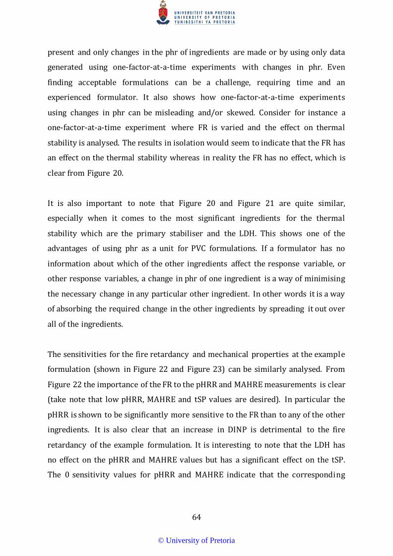
64

present and only changes in the phr of ingredients are made or by using only data

generated using one-factor-at-a-time experiments with changes in phr. Even

finding acceptable formulations can be a challenge, requiring time and an

experienced formulator. It also shows how one-factor-at-a-time experiments

using changes in phr can be misleading and/or skewed. Consider for instance a

one-factor-at-a-time experiment where FR is varied and the effect on thermal

stability is analysed. The results in isolation would seem to indicate that the FR has

an effect on the thermal stability whereas in reality the FR has no effect, which is

clear from Figure 20.

It is also important to note that Figure 20 and Figure 21 are quite similar,

especially when it comes to the most significant ingredients for the thermal

stability which are the primary stabiliser and the LDH. This shows one of the

advantages of using phr as a unit for PVC formulations. If a formulator has no

information about which of the other ingredients affect the response variable, or

other response variables, a change in phr of one ingredient is a way of minimising

the necessary change in any particular other ingredient. In other words it is a way

of absorbing the required change in the other ingredients by spreading it out over

all of the ingredients.

The sensitivities for the fire retardancy and mechanical properties at the example

formulation (shown in Figure 22 and Figure 23) can be similarly analysed. From

Figure 22 the importance of the FR to the pHRR and MAHRE measurements is clear

(take note that low pHRR, MAHRE and tSP values are desired). In particular the

pHRR is shown to be significantly more sensitive to the FR than to any of the other

ingredients. It is also clear that an increase in DINP is detrimental to the fire

retardancy of the example formulation. It is interesting to note that the LDH has

no effect on the pHRR and MAHRE values but has a significant effect on the tSP.

The 0 sensitivity values for pHRR and MAHRE indicate that the corresponding


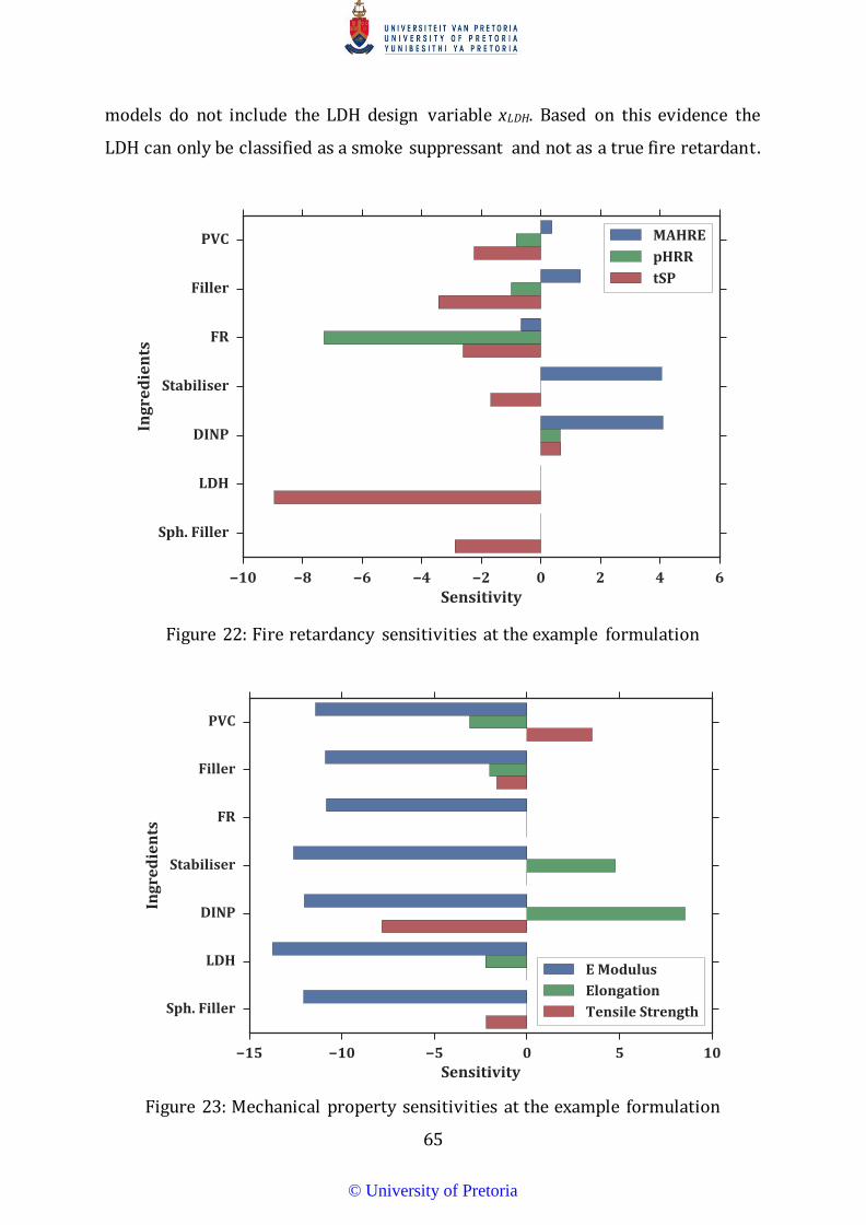
65

models do not include the LDH design variable xLDH. Based on this evidence the

LDH can only be classified as a smoke suppressant and not as a true fire retardant.

Figure 22: Fire retardancy sensitivities at the example formulation

Figure 23: Mechanical property sensitivities at the example formulation


66

The interpretation of the elongation and tensile strength sensitivities shown in

Figure 23 is simple. It shows how the DINP increases elongation and decreases

tensile strength while the PVC has exactly the opposite effect. It also shows how all

of the inorganic additives (except the FR which has no effect) have a negative effect

on at least one of the two mechanical properties. This shows for instance that the

LDH cannot be used without considering the probable adverse effects on the

elongation at break of the material. The interpretation of the sensitivities for E is

not as straight forward when considering the mixture constraint. Since E is almost

equally sensitive to all of the ingredients the change in E is based on the relative

sensitivities of all of the ingredients that change (with a minimum number of two

ingredients changing). For instance if a small increase in the mass fraction of DINP

in the example formulation is made and the mass fraction of Filler is decreased

accordingly so that the mixture constraint is maintained, E will decrease (i.e. the

compound will become more flexible). In this case it is easier to see the effect of

increasing or decreasing a certain ingredient by examining the change in the

response variable introduced by increasing the phr of that ingredient as was done

for Figure 21. This is shown in Figure 24.

It is clear that the actual change in the response variable E introduced by an

increase of 1 phr in each ingredient (Figure 24) looks quite different to the

sensitivities of E (Figure 23). This demonstrates how the sensitivities need to be

considered together for a real change in the formulation. For elongation and

tensile strength the two figures are quite similar due to the fact that the differences

in the ingredient sensitivities are more pronounced.


67

Figure 24: Change in y* for mechanical properties induced by a 1 phr change for

each ingredient

5.3 Optimisation

Analysing each response variable using the model statistics is useful. Optimisation

on the other hand can be used to analyse the entire system, as well as its more

obvious function of finding an optimum solution for a given set of conditions.

5.3.1 Optimum Solution

The optimisation can be summarised as follows: minimise

𝑓𝑓 = �𝑐𝑐𝑚𝑚𝑥𝑥𝑚𝑚

7

𝑚𝑚=1

(11)


68

subject to

�𝑥𝑥𝑚𝑚

7

𝑚𝑚=1

= 1 (12)

0 ≤ 𝑥𝑥𝑚𝑚 ≤ 1 𝑖𝑖 = 1, 2, … , 7 (13)

𝑔𝑔(𝒙𝒙) ≥ 𝑝𝑝𝑙𝑙𝑚𝑚𝑚𝑚 (15)

𝑔𝑔(𝒙𝒙) ≤ 𝑝𝑝𝑙𝑙𝑚𝑚𝑚𝑚 (16)

0.4 ≤ 𝑥𝑥𝑃𝑃𝑃𝑃𝑃𝑃 (24)

𝑥𝑥𝑓𝑓𝑚𝑚𝑙𝑙𝑙𝑙 ≤ 0.7𝑥𝑥𝑃𝑃𝑃𝑃𝑃𝑃 (25)

𝑥𝑥𝐹𝐹𝐹𝐹 ≤ 0.2𝑥𝑥𝑃𝑃𝑃𝑃𝑃𝑃 (26)

0.02𝑥𝑥𝑃𝑃𝑃𝑃𝑃𝑃 ≤ 𝑥𝑥𝑠𝑠𝑖𝑖𝑡𝑡𝑡𝑡 ≤ 0.1𝑥𝑥𝑃𝑃𝑃𝑃𝑃𝑃 (27)

0.2𝑥𝑥𝑃𝑃𝑃𝑃𝑃𝑃 ≤ 𝑥𝑥𝐷𝐷𝐷𝐷𝐷𝐷𝑃𝑃 ≤ 0.7𝑥𝑥𝑃𝑃𝑃𝑃𝑃𝑃 (28)

𝑥𝑥𝐿𝐿𝐷𝐷𝐿𝐿 ≤ 0.15𝑥𝑥𝑃𝑃𝑃𝑃𝑃𝑃 (29)

𝑥𝑥𝑠𝑠𝑠𝑠ℎ. 𝑓𝑓𝑚𝑚𝑙𝑙𝑙𝑙 ≤ 0.2𝑥𝑥𝑃𝑃𝑃𝑃𝑃𝑃 (30)

The details for equations 11 to 16 are found in section 3. Equations 24 to 30, which

represent the limits to the design space for the experimental design, are included

so that extrapolation of the empirical models is not possible. The objective

depends on the values that are used for the ingredient costs c and the limits on the

material properties plim. In reality the costs of the ingredients vary depending on

their availability and the size of the order or contract etc. The costs used here are

based broadly on the expected costs of the various ingredients to give a realistic

demonstration of the optimisation. Note that since the LDH is not a commercial

product a rough cost estimate is used. The estimated costs that are used are shown

in Table 8.

The limits on the properties are also estimated, taking into account the

requirements for underground mine cables outlined in section 2.1.2.1. An

experienced PVC formulator would be able to determine more exactly what the

required property settings should be. For this example only the most relevant

response variables, using the most comprehensive measuring technique, are


69

limited. The limits used as well as the maximum and minimum measured values

and k-fold score for each of the selected response variable is shown in Table 9.

Table 8: Estimated costs for PVC formulation ingredients

Ingredient Cost (R/kg) PVC 15 Filler 8 FR 48 Stabiliser 45 DINP 30 LDH 40 Spherical Filler 3

Table 9: Property limits for optimisation including the range of measured values

and k-fold scores

Equipment Response Variable Max Min plim k-fold Score

Torque Rheometer

Stability Time (min) 141.4 8.5 ≥25 0.58 Final Degradation Time (min) 346.9 12.6 ≥80 0.57

Cone Calorimeter

MARHE (kW/m2) 179.2 12.1 ≤85 0.89 pHRR (kW/m2) 242.8 60.0 ≤125 0.7

Tensile Test

E (MPa) 1917.7 23.6 ≤300 0.86 Elongation at Break (%) 114.8 9.8 ≥50 0.92 Tensile Strength at Break (MPa) 29.5 10.6 ≥18 0.92

The range of the measured values is shown to provide some context for the limit

values. The k-fold scores are shown because it is important to take into account

the accuracy of the model prediction when setting the property limits. This is due

to the fact that optimisation by its nature will push against the active constraints.

This means, for instance, that the predicted final degradation time of the optimum

solution is likely to be 80 min. However the model describing the final degradation

time has a k-fold score of 0.57 which is not particularly high. This means that there

is an associated prediction error and that it is distinctly possible that the real final

degradation time for the optimum formulation is less than 80 min. To avoid this

safety factors need to be introduced in the property limits and the required size of


70

the safety factors can be gaged using the k-fold score. For instance, the elongation

and tensile strength at break are predicted very well, both having a k-fold score of

0.92 (the highest possible score being 1), which means significantly lower safety

factors are required.

The optimum solution is found using a constrained non-linear optimisation

algorithm called Sequential Least Squares Quadratic Programming (SLSQP).

Multiple starts are used, with randomly generated x0 values for each start, to

increase the chance of finding the global optimum. The optimum solution for the

settings shown in Table 8 and Table 9 is shown in Table 10. All the response

variable values are shown in Table 11 with the response variables which are

included in the constraints and the values which are constrained in bold.

Table 10: Example optimum formulation

Ingredient Mass Fraction (%) phr PVC 53.19 100.0 Filler 3.34 6.3 FR 10.04 18.9 Stabiliser 1.06 2.0 DINP 18.99 35.7 LDH 2.73 5.1 Spherical Filler 10.64 20.0 Objective Function (R/kg) 20.65

Table 11: Response variable values at the example optimum solution

Equipment Response Variable Max Min Value k-fold Score

Torque Rheometer

Stability Time (min) 141.4 8.5 32.2 0.58 Final Degradation Time (min) 346.9 12.6 80.0 0.57 Resting Torque (N·m) 8.7 -1.9 3.9 0.61

Thermomat Stability Time (min) 451.4 0.0 50.6 0.41 Colour YI 140.8 -4.9 44.7 0.63 Cone Calorimeter

MARHE (kW/m2) 179.2 12.1 85.0 0.89 pHRR (kW/m2) 242.8 60.0 125.0 0.70 t to pHRR (s) 460.0 25.0 132.1 0.65


71

Equipment Response Variable Max Min Value k-fold Score

t to Ignition (s) 216.0 13.0 58.5 0.36 tHR (MJ/m2) 56.6 6.3 29.6 0.76 tSP (m2) 18.1 3.7 12.5 0.66

LOI - 37.7 23.2 35.4 0.91 MCC pHRR 1 (W/g) 388.3 85.7 245.3 0.88

pHRR 2 (W/g) 92.6 54.0 71.6 0.75 tHR (kJ/g) 20.0 10.1 12.7 0.85 tHR Peak 1 (kJ/g) 12.4 3.7 6.1 0.96 tHR Peak 2 (kJ/g) 8.9 5.2 7.3 0.35 T pHRR 1 (°C) 294.9 248.3 249.3 0.78 T pHRR 2 (°C) 467.9 451.9 455.8 0.35 t to pHRR 1 (s) 314.0 228.5 250.6 0.24 t to pHRR 2 (s) 506.5 426.5 466.4 0.00

Tensile Test

E (MPa) 1917.7 23.6 149.1 0.86 Elongation at Break (%) 114.8 9.8 50.0 0.92 Tensile Strength at Break (MPa) 29.5 10.6 19.5 0.92

Table 11 allows for the inspection of all of the response variable values at the

optimum formulation. If a value which is currently not constrained is not

satisfactory a limit on that value can simply be included. Note however that adding

constraints, if they are active, will always lead to an increase in the objective

function. It is also important to note that it is possible that adding or increasing a

constraint will mean that there is no solution, in which case the constraints need

to be relaxed.

It is interesting to note that for the above case the constraints

𝑥𝑥𝑠𝑠𝑠𝑠ℎ. 𝑓𝑓𝑚𝑚𝑙𝑙𝑙𝑙 ≤ 0.2𝑥𝑥𝑃𝑃𝑃𝑃𝑃𝑃 (30)

0.02𝑥𝑥𝑃𝑃𝑃𝑃𝑃𝑃 ≤ 𝑥𝑥𝑠𝑠𝑖𝑖𝑡𝑡𝑡𝑡 (27)

are active. This indicates that if the models are extrapolated it is possible to further

reduce f by including more spherical filler or less primary stabiliser. This will be

further discussed in the following section.


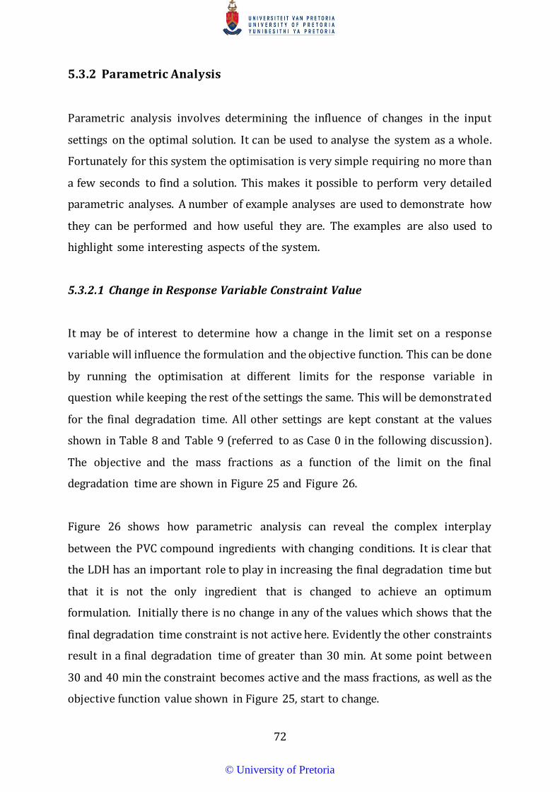
72

5.3.2 Parametric Analysis

Parametric analysis involves determining the influence of changes in the input

settings on the optimal solution. It can be used to analyse the system as a whole.

Fortunately for this system the optimisation is very simple requiring no more than

a few seconds to find a solution. This makes it possible to perform very detailed

parametric analyses. A number of example analyses are used to demonstrate how

they can be performed and how useful they are. The examples are also used to

highlight some interesting aspects of the system.

5.3.2.1 Change in Response Variable Constraint Value

It may be of interest to determine how a change in the limit set on a response

variable will influence the formulation and the objective function. This can be done

by running the optimisation at different limits for the response variable in

question while keeping the rest of the settings the same. This will be demonstrated

for the final degradation time. All other settings are kept constant at the values

shown in Table 8 and Table 9 (referred to as Case 0 in the following discussion).

The objective and the mass fractions as a function of the limit on the final

degradation time are shown in Figure 25 and Figure 26.

Figure 26 shows how parametric analysis can reveal the complex interplay

between the PVC compound ingredients with changing conditions. It is clear that

the LDH has an important role to play in increasing the final degradation time but

that it is not the only ingredient that is changed to achieve an optimum

formulation. Initially there is no change in any of the values which shows that the

final degradation time constraint is not active here. Evidently the other constraints

result in a final degradation time of greater than 30 min. At some point between

30 and 40 min the constraint becomes active and the mass fractions, as well as the

objective function value shown in Figure 25, start to change.


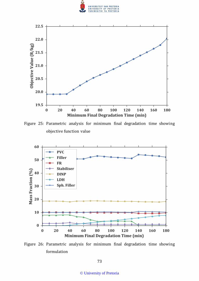
73

Figure 25: Parametric analysis for minimum final degradation time showing

objective function value

Figure 26: Parametric analysis for minimum final degradation time showing

formulation


74

Closer inspection reveals that initially, after the constraint has become active, the

final degradation time is increased by increasing the primary stabiliser. This is

shown more clearly in Figure 27.

Figure 27: Parametric analysis for minimum final degradation time (30 – 50 min)

showing selected ingredient mass fractions

After the initial increase of the primary stabiliser, the amount of LDH is increased

while the primary stabiliser increases only slightly. Then between 42.5 and 45 min

the amount of primary stabiliser suddenly drops and starts to decrease. Complex

behaviour such as this can only be revealed by taking into account the entire

system.

Note also that the constraints from the experimental design are active at different

points of the parametric analysis. The upper limit on the spherical filler seems to

be active regardless of the minimum final degradation time. This is evident by the

fact that it changes proportionally to the change in the PVC. If the constraints on


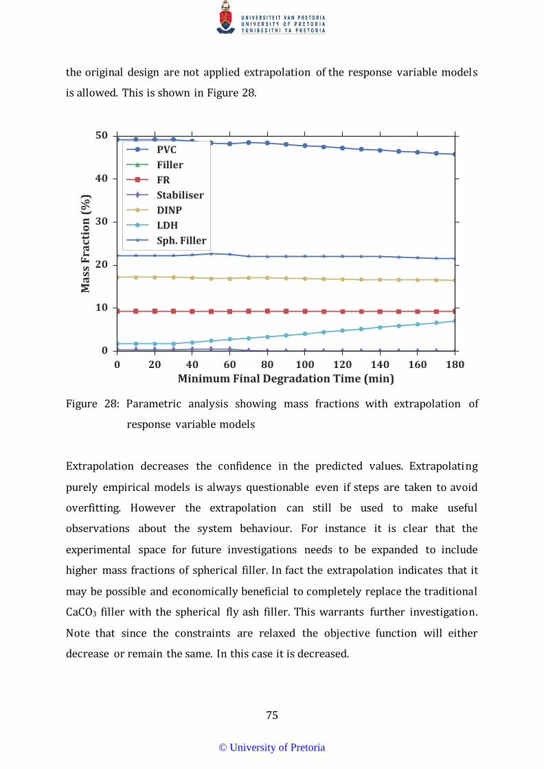
75

the original design are not applied extrapolation of the response variable models

is allowed. This is shown in Figure 28.

Figure 28: Parametric analysis showing mass fractions with extrapolation of

response variable models

Extrapolation decreases the confidence in the predicted values. Extrapolating

purely empirical models is always questionable even if steps are taken to avoid

overfitting. However the extrapolation can still be used to make useful

observations about the system behaviour. For instance it is clear that the

experimental space for future investigations needs to be expanded to include

higher mass fractions of spherical filler. In fact the extrapolation indicates that it

may be possible and economically beneficial to completely replace the traditional

CaCO3 filler with the spherical fly ash filler. This warrants further investigation.

Note that since the constraints are relaxed the objective function will either

decrease or remain the same. In this case it is decreased.


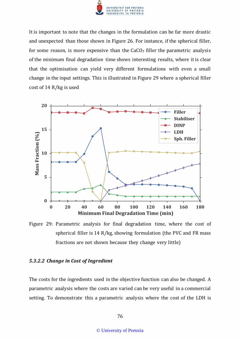
76

It is important to note that the changes in the formulation can be far more drastic

and unexpected than those shown in Figure 26. For instance, if the spherical filler,

for some reason, is more expensive than the CaCO3 filler the parametric analysis

of the minimum final degradation time shows interesting results, where it is clear

that the optimisation can yield very different formulations with even a small

change in the input settings. This is illustrated in Figure 29 where a spherical filler

cost of 14 R/kg is used

Figure 29: Parametric analysis for final degradation time, where the cost of

spherical filler is 14 R/kg, showing formulation (the PVC and FR mass

fractions are not shown because they change very little)

5.3.2.2 Change in Cost of Ingredient

The costs for the ingredients used in the objective function can also be changed. A

parametric analysis where the costs are varied can be very useful in a commercial

setting. To demonstrate this a parametric analysis where the cost of the LDH is


77

changed will be analysed. The parametric analysis is shown in Figure 30 and

Figure 31.

Figure 30: Parametric analysis of LDH cost showing the objective value

Figure 31: Parametric analysis of LDH cost showing ingredient mass fractions


78

For a PVC formulator or cable manufacturer an analysis of the following type can

be used to determine the impact of a change in the cost of the LDH on the

production cost and optimum formulation. For a manufacturer of the LDH the

parametric analysis can be used, for instance, as a tool to determine the

appropriate selling price of the LDH.

Consider for example the hypothetical situation where a manufacturer of the LDH

is negotiating a contract to supply LDH to a compounder, who needs to

manufacture a set mass of PVC compound using the ingredients used in this study.

In this case the total profit depends on both the profit margin on the LDH and on

how much LDH the compounder uses. This can be expressed by multiplying the

profit margin of the LDH by the mass fraction of the LDH used in the optimum

formulation to determine the profit per kg required by the supplier. This is shown,

using a hypothetical production cost of 10 R/kg for the LDH, in Figure 32.

Figure 32: Parametric analysis on LDH cost showing hypothetical profit


79

Figure 32 shows that for this example it is possible to sell the LDH at 15 R/kg or

25 R/kg and make the same amount of profit. This is due to the fact that there is a

point where the amount of LDH included in the optimum formulation is drastically

reduced. From Figure 30 it is clear that the overall cost of the PVC compound is

significantly lower at 15 R/kg than 25 R/kg. In the hypothetical example the LDH

manufacturer can present the compounder with a much more attractive offer at

15 R/kg than 25 R/kg while making the same amount of profit. The sudden

decrease in the amount of LDH included in the formulation (and the other

associated changes in the formulation) can be attributed to the point where the

LDH becomes more expensive than the PVC resin, which has a cost of 15 R/kg. This

shows the importance of the ingredient costs relative to each other.

Even though the above example is crude (in particular using an unrealistically low

cost of production for the LDH) it demonstrates how parametric analysis can be

used to make important decisions, taking into account the entire system

behaviour. It is also important to note that parametric analysis of this system is

not restricted to two dimensions, or what is effectively a one-factor-at-a-time

approach, as was used for the above examples. This was done simply to

demonstrate the principle and to make the interpretation of the analysis simpler.

It is also important to note that in a commercial setting the exact values used for

the input settings are important. It is recommended that accurate values for the

ingredient costs and required response variable settings for flexible PVC

underground mine cable insulation are researched. It is further recommended that

parametric analyses are conducted that address specific industry relevant

questions.

5.3.2.3 Change in Response Variables Constrained

The response variables that are constrained can also be changed. This is of interest

for this study due to the different methods used to measure the thermal stability


80

and the fire retardancy. In terms of thermal stability the values for Thermomat

stability time and YI are both satisfactory for Case 0 where the Torque Rheometer

final degradation time is constrained. This shows that the measurements are

linked. However if the Torque Rheometer response variables are not constrained

and instead only the Thermomat stability time is constrained the long term

thermal stability (final degradation time) is no longer satisfactory. The

optimisation results for this case (referred to as Case 1), with the Thermomat

stability time constrained to a minimum of 55 min, are shown in Table 12 and

Table 13

Table 12: Optimum formulation with constraining Thermomat rather than Torque

Rheometer Measurements

Mass Fraction (%) Ingredient Case 0 Case 1 PVC 53.19 52.07 Filler 3.34 6.76 FR 10.04 10.19 Stabiliser 1.06 1.56 DINP 18.99 19.01 LDH 2.73 0 Spherical Filler 10.64 10.41 Objective Function (R/kg) 20.65 19.96

Table 13: Response variable values for thermal stability

Equipment Response Variable Value k-fold

Score Case 0 Case 1 Torque Rheometer

Stability Time (min) 32.2 19.2 0.58 Final Degradation Time (min) 80.0 27.07 0.57 Resting Torque (N·m) 3.9 4.2 0.61

Thermomat Stability Time (min) 50.6 55.0 0.41 Colour YI 44.7 10.2 0.63

It is clear that the Thermomat stability time is not a complete representation of the

thermal stability behaviour. This is expected due to the fact that it is a static and


81

not a dynamic test like the Torque Rheometer. It fails to capture the long term

stabilising abilities of the LDH so that it is not included in the formulation. The YI

can also be shown to be an insufficient measure of long term thermal stability.

The different measurement techniques for fire retardancy can be similarly

investigated. It is of particular interest to determine if the less time consuming and

complicated LOI and MCC measurements are sufficient to describe the fire

retardancy of the system. However this requires a more detailed investigation of

the system beyond the scope of this report, but is recommended for future work

due to the fact that the data set is well suited to such an investigation.

5.4 Implementation

All of the calculations and analyses described in sections 5.1 to 5.3 were done using

code written in Python programming language using IPython Interactive

Computing (Perez & Granger, 2007). The model validation was done using scikit-

learn (Pedregosa, et al., 2011) and the model statistics were calculated using

Statsmodels (Seabold & Perktold, 2010). The optimisation of the system was done

using SciPy (Millman & Aivazis, 2011). All the code is available online at

https://github.com/reinhardfechter/FlexPVCModel.

5.5 Labour and Time Savings

The usefulness of the models, determined using statistical experimental design, is

demonstrated extensively in the previous sections. Another important aspect of

using statistical experimental design, that has not been highlighted, is the

efficiency with which it uses experimental data. This is important due to the fact

that real experiments will always use resources i.e. there will always be an

associated cost of performing the experiments.


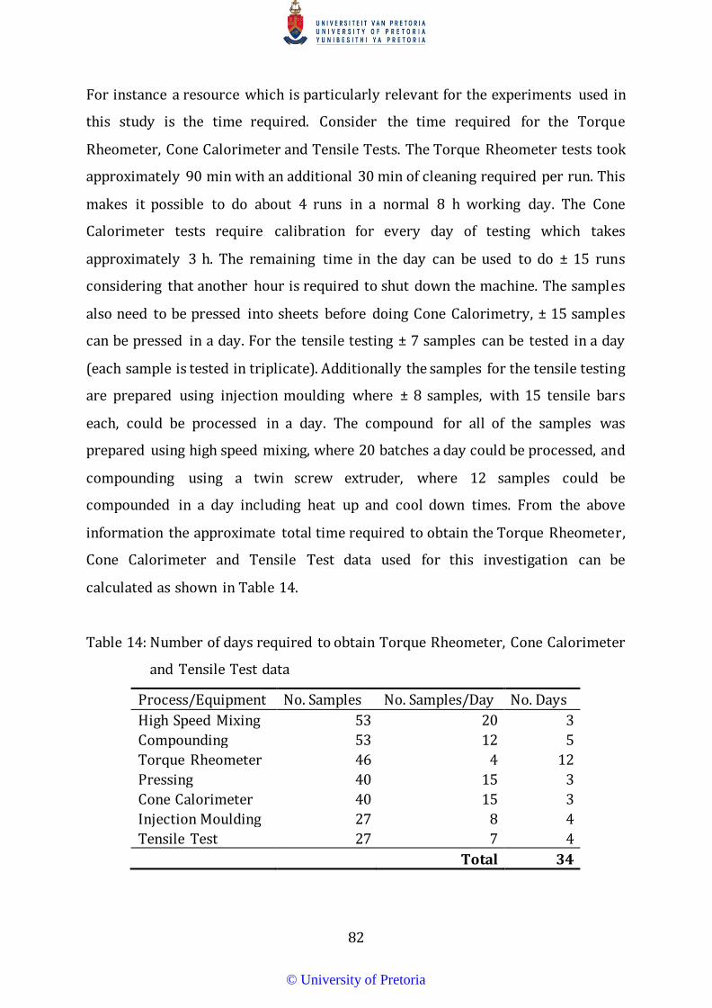
82

For instance a resource which is particularly relevant for the experiments used in

this study is the time required. Consider the time required for the Torque

Rheometer, Cone Calorimeter and Tensile Tests. The Torque Rheometer tests took

approximately 90 min with an additional 30 min of cleaning required per run. This

makes it possible to do about 4 runs in a normal 8 h working day. The Cone

Calorimeter tests require calibration for every day of testing which takes

approximately 3 h. The remaining time in the day can be used to do ± 15 runs

considering that another hour is required to shut down the machine. The samples

also need to be pressed into sheets before doing Cone Calorimetry, ± 15 samples

can be pressed in a day. For the tensile testing ± 7 samples can be tested in a day

(each sample is tested in triplicate). Additionally the samples for the tensile testing

are prepared using injection moulding where ± 8 samples, with 15 tensile bars

each, could be processed in a day. The compound for all of the samples was

prepared using high speed mixing, where 20 batches a day could be processed, and

compounding using a twin screw extruder, where 12 samples could be

compounded in a day including heat up and cool down times. From the above

information the approximate total time required to obtain the Torque Rheometer,

Cone Calorimeter and Tensile Test data used for this investigation can be

calculated as shown in Table 14.

Table 14: Number of days required to obtain Torque Rheometer, Cone Calorimeter

and Tensile Test data

Process/Equipment No. Samples No. Samples/Day No. Days High Speed Mixing 53 20 3 Compounding 53 12 5 Torque Rheometer 46 4 12 Pressing 40 15 3 Cone Calorimeter 40 15 3 Injection Moulding 27 8 4 Tensile Test 27 7 4 Total 34


83

Consider a hypothetical situation where a formulator wishes to find an optimum

formulation of the same system, using only the traditional one-factor-at-a-time

experiments with changes in phr and a sequential next-best-guess approach.

There is a set requirement for the thermal stability, fire retardancy and tensile test

that needs to be reached. Say the formulator uses a known formulation as a

starting point. The properties are then ordered and a certain core ingredient to

change for each property is selected. Say the LDH for stability, the FR for fire

retardancy and the DINP for the mechanical property are selected.

The phr of LDH in the formulation is changed first. For example say that 5

additional formulations are used with each formulation tested using the torque

rheometer. Since the torque rheometer is known to have a high variance the

formulator uses triplicate measurements on each formulation therefore requiring

18 runs. Since only the phr of LDH is changed (and not that of the DINP) only one

batch of high speed mixing (i.e. making one dry mix) is required. The formulator

analyses the results and chooses a new base formulation satisfying the thermal

stability requirement. If the formulator is prudent a formulation with a thermal

stability that is slightly higher than the requirement is selected. The formulator

then repeats the above process for the FR and Cone Calorimeter experiments and

the DINP and tensile experiments.

The formulator then decides to increase the Filler amount to decrease the overall

cost of the formulation having fulfilled the material requirements by running one-

factor-at-a-time experiments for all three response variables, again with 5

additional formulations measured in triplicate. A new base formulation is again

chosen such that the material requirements are still achieved. This is repeated

with the Spherical Filler. The process described above is summarised in Table 15

including a calculation of the approximate amount of time required.


84

Table 15: Number of experiments and amount of time required for example of

next-best-guess approach using one-factor-at-a-time experiments

Process/Equipment

No. of Runs/Batches No. Samples /Day

No. Days LDH FR DINP Filler

Sph. Filler Total

High Speed Mixing 1 6 1 8 20 1 Compounding 6 6 6 6 6 30 12 3 Torque Rheometer 18 18 18 54 4 14 Pressing 18 18 18 54 15 4 Cone Calorimeter 18 18 18 54 15 4 Injection Moulding 18 18 18 54 8 7 Tensile Test 18 18 18 54 7 8 Total 41

At this point in the hypothetical example more time has already been spent than

what is shown in Table 14 (i.e. what was approximately required in this

investigation for the measurements used in the example). At best the formulator

has found an improved formulation (i.e. with a lower cost) which satisfies the

requirements. This formulation is, however, highly unlikely to be the optimum

formulation. To find the optimum formulation would require many more

iterations of the type of processes described above, and even if the optimum is

found it is difficult to prove that it is indeed the optimum using data generated in

this way. In addition to this if the property requirements are subsequently

changed a portion if not the entire experimental process needs to be repeated. In

summary the proper use of optimisation and statistical experimental design not

only makes it possible to find an optimum formulation for a range of different

requirements, it also requires significantly less labour and time to get to an

optimum solution.


85

6 Conclusions and Recommendations

6.1 Response Variable Models

It can be concluded that the response variables describing the thermal stability,

fire retardancy and basic mechanical properties as a function of the mass fractions

of the PVC compound ingredients (i.e. the formulation) can be modelled effectively

using 2nd order Scheffé polynomials. The particular empirical models for each

response variable, selected and evaluated for predictive ability using k-fold cross

validation, can be interpreted using statistics to make deductions about the

relationship between the response variables and the formulation. The interaction

terms in the 2nd order Scheffé polynomial are particularly useful in identifying

synergistic and antagonistic relationships between ingredients.

This principle is demonstrated using the model selected to describe the final

degradation time measured by the torque rheometer. The model shows clearly

that there is a synergistic relationship between DINP and the LDH which has the

greatest influence on the final degradation time. The DINP itself is shown to have

a negative effect and additional weaker synergistic effects with the spherical filler

and primary stabiliser. The spherical filler and LDH similarly show a negative

effect in isolation however there is evidence that supports the hypothesis that they

are synergists. Finally it is interesting to note that there is relatively strong

evidence of antagonism between the LDH and primary stabiliser which is contrary

to what is reported in literature. These conclusions show the value of using

statistical experimental design over the one-factor-at-a-time experiments

favoured in the literature on LDH as a PVC additive. It is recommended that a

detailed statistical analysis of all the response models is conducted and that

previously unreported interactions and effects, including those described above

are investigated further.


86

The interaction terms in the models mean that the effect of a certain ingredient is

dependent on the mass fractions of the other ingredients. Sensitivity analysis can

be used to determine the overall effect of a very small independent change in the

mass fraction of an ingredient on a response variable at a given formulation.

Sensitivity analyses of selected response variables at an example formulation,

based on an existing commercial cable formulation, are used as a demonstration.

The example sensitivity analysis for the long and short term thermal stability

shows the strong influence of the primary stabiliser and the LDH. It also shows

how the primary stabiliser has a stronger influence on short term stability while

the LDH has a stronger influence on long term stability. The sensitivity analysis

shows that an increase in the stabiliser for the example formulation leads to an

increase in long term stability in spite of the antagonism between the LDH and the

stabiliser. This demonstrates how sensitivity analysis gives insight into the model

behaviour which is not necessarily clear from the statistical analysis of the model

parameters.

The sensitivity analyses for the fire retardancy of the example formulation shows

that the FR is the most important ingredient in terms of reducing the pHRR and

MAHRE values. It also shows that an increase in the DINP has a detrimental effect

on fire retardancy. Interestingly the LDH only has an effect on the tSP value, which

means that in this case the LDH can only be classified as a smoke suppressant and

not as a true fire retardant. The sensitivity analysis of the mechanical properties

shows how the DINP increases elongation and decreases tensile strength while the

PVC has exactly the opposite effect. It also shows how all of the inorganic additives

(except the FR which has no effect) have a negative effect on at least one of the two

mechanical properties. This shows for instance that the LDH cannot be used

without considering the likely adverse effects that it has on the elongation at break.

It is important, however, to understand that the independent change in the amount

of an ingredient, shown by the sensitivity analysis, is not possible for a mixture due


87

to the mixture constraint. When making a real change to the mass fraction of a

certain ingredient the mass fraction of at least one other ingredient must also

change to maintain the mixture constraint. Therefore, for a real change in the

formulation, the sensitivities of at least two ingredients need to be taken into

account.

This is particularly important when making adjustments to a formulation in the

traditional units of phr. This is due to the fact that a change in phr of an ingredient

relates to an increase in the mass fraction of the ingredient in question while the

mass fractions of the remaining ingredients are decreased together, to a lesser

extent, with only their ratios maintained. This is why, for instance, a change in the

phr of the FR in the example formulation, will have an effect on the thermal

stability even though, according to the sensitivity analysis, the FR itself has no

effect. These unwanted changes make it near impossible for a person to find an

optimum formulation when multiple response variable requirements are present

and only changes in the phr of ingredients are made or by using only data

generated using one-factor-at-a-time experiments with changes in phr. Even

finding acceptable formulations can be a challenge, requiring time and an

experienced formulator. It also shows how one-factor-at-a-time experiments

using changes in phr can be misleading and/or skewed. If, however, a formulator

has no information about which of the other ingredients affect the response

variable or other response variables, a change in phr of one ingredient is a way of

minimising the necessary change in any particular other ingredient.

6.2 Optimisation

It can also be concluded that the models make it possible to minimise the cost of

the PVC compound by varying the formulation. The optimum formulation is a

function of the costs of the various ingredients and the limits which are placed on

the response variables. To analyse the system as a whole, parametric analysis can


88

be used. The number of different analyses which can be done is very large and

depend on the specific questions which need to be answered. Some basic analyses

demonstrate the usefulness of parametric analysis and highlight some interesting

aspects of the system.

The value of the limit on a response variable can be changed. An analysis of this

type, where the Torque Rheometer final degradation time is varied, reveals the

complex interplay between the PVC compound ingredients with changing

conditions. The analysis shows that initially there is no change in the formulation

because the final degradation time constraint is not active. Then at 40 min the

constraint becomes active, indicated by a change in the formulation. Initially the

final degradation time is increased by increasing the amount of primary stabiliser.

Then the LDH is introduced and increased steadily while the primary stabiliser is

still increased but to a lesser degree. At some point between 42.5 and 45 min the

amount of primary stabiliser suddenly drops and starts to decrease. Complex

behaviour such as this can only be revealed by taking into account the entire

system.

It is also noted that the constraints from the experimental design are active at

certain points of the parametric analysis. Repeating the parametric analysis

described above without the experimental space constraints, i.e. allowing the

models to extrapolate, indicates that it may be possible and economically

beneficial to completely replace the traditional CaCO3 filler with the spherical fly

ash filler. It is recommended that an expanded experimental space allowing for

higher mass fractions of spherical filler is investigated.

A similar parametric analysis is conducted where the cost of the LDH is varied. The

analysis shows how the formulation changes drastically, in particular decreasing

the amount of LDH used, when the LDH cost becomes larger than the resin cost. It

is shown using a hypothetical situation that a quantitative description of such


89

behaviour can be used to make informed commercial decisions, which take into

account the complex behaviour of the system in question. To make conclusions

that are more directly relevant to industry it is recommended that the exact input

settings for the optimisation are researched. It is then recommended that

parametric analyses are designed that answer specific questions relevant to the

industry.

The parametric analysis on this system can also be used to determine the

completeness of the different measuring techniques used to describe the thermal

stability and fire retardancy of the PVC compound. It is demonstrated that the

Torque Rheometer is the only measuring technique for thermal stability, of those

used in this study, to differentiate between the long term and short term stability.

This means, for instance, that it is the only measuring technique which can capture

the long term stabilising effects of LDH. The different measurement techniques for

fire retardancy can be similarly investigated. It is recommended that a detailed

investigation comparing the different measuring techniques is conducted using

the data collected for this investigation.

Finally it can be concluded that using proper statistical experimental design over

the traditional one-factor-at-a-time experiments leads to significant time and

labour savings. This is due to the efficiency with which statistical experimental

design uses experimental data.


90

7 Future Work

Some recommendations for future work, based directly on the conclusions, have

already been made in the previous section. Additional recommendations for future

work based on the broader outcomes of this investigation are discussed here.

The analysis of the data as it is presented in this report (i.e. by using optimisation)

has been implemented using code written in Python programming language. This

means that in its current state the analysis of the data, and hence the data itself, is

inaccessible to anyone that is unfamiliar with how to manipulate or run code

written in Python programming language (or does not have the time to figure out

how the code works).

To make the analysis of the data accessible and usable, for anyone with a basic

understanding of the system under study and the analysis methods used, requires

an interface. For example, a simple interface could be designed that allows a user

to change the mass fractions of the 7 ingredients and observe the resultant

material properties, which are calculated in the background using the empirical

models. This will allow a user to ‘play around’ with different formulations and

observe how the material properties change. It is important to note however that

a mechanism is required that makes sure that the mixture constraint is

maintained. One way to do this is to allow the user to make changes in the phr of

the various additives which can then be converted to mass fractions by the

program. This is also a more familiar unit for anyone who has worked with PVC

formulations and/or research before.

Additionally the interface would allow the user to enter the costs of each

ingredient, select which material properties should be constrained and what the

value of the limits should be. The user would then be able to press a button which

performs the optimisation and displays the optimum formulation, the material


91

properties of the formulation and the objective function value (unless no optimum

solution could be found in which case an appropriate error message should be

displayed). This basic idea can be modified further depending on specific user

requirements. Examples of this would be to make comparisons between different

formulations easier or to allow the user to conduct parametric analyses such as

those shown in section 5.3.2.

All the recommendations for future work made up until this point (except the

recommendation to expand the experimental space to include more spherical

filler) do not require any additional physical experiments. However, with the

current data set, it is only possible to find an optimum formulation, or make

definitive conclusions about the behaviour of the mixture, within the experimental

space. For the recommendation to investigate higher mass fractions of spherical

filler the experimental space can be expanded by simply conducting some

additional experiments using the same 7 ingredients used in this investigation. If,

however, a researcher or formulator is interested in investigating one or more new

ingredients there will be new terms in the Scheffé models, which need to be taking

into account.

For instance say a formulator is interested in the same system that was

investigated here, except that a different LDH is to be investigated. For this new

investigation only enough experiments are required to determine the additional

model terms, which include the linear term for the new LDH and the interaction

terms of the new LDH with the 6 other ingredients (i.e. the PVC, filler, FR, DINP,

stabiliser and spherical filler, assuming that a 2nd order Scheffé polynomial is

used). The other terms that do not involve the new LDH have already been

determined in this investigation and do not need to be determined again. If the

same validation strategy is used, i.e. using k-fold cross validation with k = 3, 11

additional experimental points (formulations) are required for the 7 new model

terms. The number of experimental points can be calculated using the equation


92

𝑁𝑁𝑒𝑒 = �𝑁𝑁𝑘𝑘

𝑘𝑘 − 1� (43)

where N is the number of terms and Ne is the number of experimental points. The

new data that is collected and the data from this investigation can then be

combined into a single data set which can be analysed using effectively the same

methods used in this investigation.

If a PVC compound that contains none of the ingredients that were used in this

investigation is of interest a new separate data set needs to be generated. This can

be done by following the same procedure which is outlined in this report. In fact

the method that is used in this investigation can be generalised to optimise the

proportions of the ingredients of any mixture.


93

8 References

Ari, G. A., 2010. Using a torque rheometer to characterize flow in poly(vinyl

chloride) composites. Plastics Research Online.

American Society for Testing and Materials, 2002. Standard Practice for Fusion of

Poly(Vinyl Chloride) Compounds Using a Torque Rheometer. ASTM D2538-02:

2002 United States of America: ASTM.

Attenberger, P. et al., 2011. Polyvinyl Chloride (PVC). Kunststoffe International.

Bacaloglu, R. & Fisch, M. H., 2000. Thermal Degradation and Stabilisation of PVC.

Munich: Hanser.

Bacaloglu, R. & Fish, M., 1995. Degredataion and stabilization of poly(vinyl

chloride). V. Reaction maechanism of poly(vinyl chloride) degradation. Polymer

Degredation and Stability, Volume 47, pp. 33 - 57.

Braun, D., 2004. Poly(vinyl chloride) on the Way from the 19th Century to the

21st Century. Journal of Polymer Science: Part A: Polymer Chemistry, Volume 42,

pp. 578-586.

Ceresana Research, 2014. Global demand for PVC to rise by about 3.2%/year to

2021. Additives for Polymers, November, pp. 10 - 11.

European Council for Vinyl Manufacturers, 2014. How is PVC used?. [Online]

Available at: http://www.pvc.org/en/p/how-is-pvc-used

[Accessed 21 October 2016].


94

Focke, W. W., van der Westhuizen, I. & Oosthuysen, X., 2016. Biodiesel oxidative

stability from Rancimat data. Thermochimica Acta, Volume 633, pp. 116-121.

Forano, T., Hibino, T., Leroux, F. & Taviot-Gueho, C., 2006. Layered Double

Hydroxides. In: F. Bergaya, B. K. G. Theng & G. Lagaly, eds. Handbook of Clay

Science. s.l.:Elsevier Ltd., pp. 1021-1070.

Grellmann, W. & Seidler, S., 2013. Polymer Testing. Munich: Hanser.

Gupta, S., Agarwal, D. D. & Banerjee, S., 2009. Thermal Stabilization of Poly(vinyl

chloride) by Hydrotalcites, Zeolites, and Conventional Stabilizers. Journal of Vinyl

& Additive Technology.

Hastie, T., Tibshirani, R. & Friedman, J., 2009. The Elements of Statistical Learning.

2nd ed. New York: Springer.

Joseph, P., Tretsiakova-McNally, S. & Zhang, R., 2016. Techniques for Assessing

the Combustion Behaviour of Polymeric Materials: Some Current Perspectives

and Future Directions. Macromolecular Symposia, Volume 362, pp. 105-118.

Joshi, H., 2008. Residential, Commercial and Industrial Electrical Systems:

Equipment and Selection. New York: McGraw Hill Education.

Khastgir, D., 2009. Polymers in Cable Application. In: J. White, S. K. De & K.

Naskar, eds. Rubber Technologist's Handbook Volume 2. Shawbury: iSmithers

Rapra, pp. 249-307.

Labuschagne, F. J. W. J., Giesekke, E. W. & van Schalkwyk, J. D., 2006. Production of

Hydrotalcite. s.l. Patent No. WO 2006/123284 A2.


95

Labuschagne, F. J. W. J. et al., 2015. Heat stabilising flexible PVC with layered

double hydroxide derivatives. Polymer Degradation and Stability, Volume 113, pp.

46-54.

Laoutid, F. et al., 2009. New prospects in flame retardant polymer materials:

From fundamentals to nanocomposites. Materials Science and Engineering R,

Volume 63, pp. 100-125.

Levchik, S. V. & Weil, E. D., 2005. Overview of the recent literature on flame

retardancy and smoke suppression in PVC. Polymers for Advanced Technologies,

Volume 16, pp. 707-716.

Lundsted, T. et al., 1998. Experimental design and optimization. Chemometrics

and intelligent laboratory systems, Volume 42, pp. 3 - 40.

Millman, K. J. & Aivazis, M., 2011. Python for Scientists and Engineers. Computing

in Science & Engineering, Volume 13, pp. 9-12.

Montgomery, D. C., 2013. Design and Analysis of Experiments. 8th ed. Hoboken:

John Wiley & Sons.

Murphy, J., 2001. Additives for Plastics Handbook. 2nd ed. New York: Elsevier.

Osswald, T. A., 2010. Understanding Polymer Processing; Processes and Governing

Equations. Munich: Hanser.

Pabla, A. P., 2011. Electric Power Distribution. 6th ed. New York: McGraw-Hill.

Pedregosa, F. et al., 2011. Scikit-learn: Machine Learning in Python. Journal of

Machine Learning Research, Volume 12, pp. 2825-2830.


96

Perez, F. & Granger, B. E., 2007. IPython: A System for Interactive Scientific.

Computing in Science and Engineering, 9(3), pp. 21-29.

SAS Institute Inc., 2015. JMP 12 Design of Experiments Guide. Cary, NC: SAS

Institute Inc.

SAS Institute Inc., 2015. JMP, Version 12.0.1. Cary, NC: s.n.

Scheffé, H., 1958. Experiments With Mixtures. Journal of the Royal Statistical

Society, 20(2), pp. 344 - 360.

Schiller, M., 2015. PVC Additives; Performance, Chemistry, Developments and

Sustainability. Munich: Hanser.

Seabold, S. & Perktold, J., 2010. Statsmodels: Econometric and statistical

modeling with python. Proceedings of the 9th Python in Science Conference, pp.

57-61.

Shoemaker, T. M. & Mack, J. E., 2012. Lineman's and Cableman's Handbook. 12th

ed. New York: McGraw-Hill.

Towler, G. & Sinnott, R., 2013. Chemical Engineering Design; Principles, Practice

and Economics of Plant and Process Design. Oxford: Elsevier.

van der Merwe, E. M. et al., 2014. Surface and bulk characterization of an

ultrafine South African coal fly ash with reference to polymer applications.

Applied Surface Science, Volume 317, pp. 73-83.


97

Wang, X. & Zhang, Q., 2004. Effect of hydrotalcite on the thermal stability,

mechanical properties, rheology and flame retardance of poly(vinyl chloride).

Polymer International, Volume 53, pp. 698-707.

Wilkes, C. E., Summers, J. W. & Daniels, C. A., 2005. PVC Handbook. 1st ed. Munich:

Hanser.

Wright, H. C., 2016. Layered double hydroxides as PVC thermal stabilisers; the

effect of particle size and concentration, Pretoria: University of Pretoria.

Wypych, G., 2008. PVC Degradation & Stabilization. 2nd ed. Toronto: ChemTec.

Wypych, G., 2009. PVC Formulary. Toronto: ChemTec.

Wypych, G., 2016. Handbook of Fillers. 4th ed. Toronto: ChemTec.


modelling and optimisation of flexib le pvc compound

Documents