modelling and forecasting exchange rates with a bayesian time-varying coefficient model

Journal of Economic Dynamics and Control 17 (1993) 233-261. North-Holland

Modelling and forecasting exchange rates with a Bayesian time-varying coefficient model

F a b i o Canova* Brown University, Providence, RI 02912, USA European University Institute, 1-50016 San Domenico di Fiesole, Italy

Received May 1990, final version received January 1992

This paper employs a multivariate Bayesian time-varying coetficients (TVC) approach to model and forecast exchange rate data. It is shown that, if used as a data-generating mechanism, a TVC model induces nonlinearities in the conditional moments and leptokurtosis in the unconditional distribution of the series. It is also shown that leptokurtic behavior disappears under time aggregation. As a forecasting device, a Bayesian TVC model improves over a random walk model. The improvements are robust to several changes in the forecasting environment.

I. Introduction

It is widely recognized that short-term changes in a variety of asset prices are well described by linearly unpredictable stochastic processes which are unconditionally leptokurtic and conditionally heteroskedastic. Studies by Meese and Rogoff (1983a, b), Domowitz and Hakkio (1985), Boothe and Glassman (1987), Hsieh (1988), and Diebold (1988) have documented that for the case of exchange rate changes (1) the conditional mean is approximately linear and nonlinearities, if they exist, arise in the even conditional moments of the process and (2) the current value of the process summarizes all the information that is relevant to forecast future values. One implication of

*I would like to thank T. Erickson, E. Leeper, J. Marrinan, and C. Sims for useful conversations, C. Engel, R. Meese, F. Diebold, G. Mizon, B. Mizrach, A. Pagan, and two anonymous referees for comments, and P. Angelini for assisting in part of the computations. A version of this paper entitled 'Are Exchanger Rates Really Random Walks?' was presented at the 1989 Winter Meeting of the Economic Society, Atlanta and at the Econometric workshop at University of Pennsylvania and at the Federal Reserve Bank of Atlanta.

0165-1889/93/$05.00 © 1993--Elsevier Science Publishers B.V. All rights reserved

234 F. Canova, Forecasting exchange rates

these findings was that a random walk (RW) model appeared to be the best tool for out-of-sample point forecasts.

The lack of predictability in asset price changes, however, is increasingly being questioned both at a theoretical and an empirical level. Theoretically, Sims (1984) argues that any price which is strongly anticipatory of future events will behave like a martingale only as the sampling interval goes to zero. Empirically, Engle, Lilien, and Robbins (1987), Pagan and Yong (1990), and Engel and Hamilton (1990), among others, have demonstrated the existence of nonlinear dependencies in the conditional mean of certain asset prices using data at various frequencies.

In an attempt to exploit these nonlinear dependencies in forecasting exchange rate changes, Diebold and Nason (1990) examine the performance of a class of univariate models where the conditional mean is allowed to be a nonlinear function of the available information set. They employ nonparametric methods to construct an estimate of the conditional mean which is, under a quadratic loss function, the best predictor of future exchange rate changes. Their results are mixed: the particular form of nonlinear dependence they employ does not necessary improve the out-of-sample forecasting performance of linear models (and of a RW model in particular). Mizrach (1990), using an analogous but multivariate technique and a different sam- piing interval, improves over a RW model in only one exchange market. Similarly, Meese and Rose (1989) show that the same class of models has only a slightly better in-sample fit than linear models over a variety of samples and situations.

This paper contributes to this emerging literature in two ways. I provide a parametric model which, if used as a data-generating mechanism, produces complex nonlinear dependencies in the conditional moments of the generated time series and can replicate several important empirical features of exchange rate data [see Gallant, Hsieh, and Tauchen (1990) for a similar undertaking using Clark's (1973) 'mixture' model]. I then demonstrate that the forecasts of this model substantially improve upon the forecasts of a RW model.

The approach of the paper differs from previous efforts in several respects. First, a Bayesian time-varying coefficient (TVC) autoregressive model of the variety pioneered by Litterman (1982), Doan, Litterman, and Sims (1984), and Sims (1989) is employed. Second, a number of foreign exchange and interest rate markets are simultaneously considered in the forecasting exercise. This approach has the advantage of employing a richer information structure and exploiting common features existing in a variety of financial markets to construct forecasts [see Diebold and Nerlove (1989) for a similar argument].

I show that the TVC methodology has several appealing features for modelling financial data. First, a TVC model is flexible enough to include as

F. Canova, Forecasting exchange rates 235

special cases several nonlinear time series specifications recently employed to model the first two conditional moments of exchange rates and of other financial data [see Tsay (1987) for some of these relationships]. Second, if used as a data-generating mechanism (DGM), the model produces nonnormalities in the endogenous time series by means of time variation in the coefficients. Time variation was found to be a relevant ingredient in ex- plaining the leptokurtic behavior of exchange rate data [Friedman and Vandersteel (1982), Boothe and Glassman (1987)] and in forecasting exchange rates with structural models [Wolff (1987), Schinasi and Swamy (1989)]. Third, the generated time series have the property that time aggregation reduces nonnormalities [see Diebold (1988) for this feature of exchange rate data]. Fourth, since the model has a linear recursive conditionally Gaussian structure [Lipster and Shiryayev (1978)], simple estimation and forecasting procedures are applicable to a vector of time series. Finally, as emphasized by Engle and Watson (1985), TVC models have a Bayesian interpretation. Therefore the information contained in various foreign exchange and interest rate markets can be pooled with a simple Bayesian procedure.

I also show that as a forecasting tool, a Bayesian TVC model is useful and improves upon RW forecasts at all horizons and for all the exchange rates considered using three different loss functions. The improvement is statistically significant, essentially independent of the time period chosen to compute forecasts and robust to various alterations in the model specification.

The rest of the paper is organized as follows: the next section describes a TVC model and examines the statistical properties of time series generated with such a model. Section 3 presents details on the forecasting exercise. Section 4 presents the forecasting results and a robustness analysis. Section 5 contains the conclusions.

2. A statistical model for exchange rate data

Consider the following data-generating mechanism (DGM):

Yt = [3',xt + u t , (1)

where u t, conditional on x t, is white noise with variance V. For the sake of presentation, I assume that Yt is a scalar stochastic process, 1 fl't is a 1 × (l + 1) vector of time-varying coefficients of the model, and x t is a (1 + 1) × 1 vector of lagged dependent or exogenous variables. I also assume that/3 t evolves according to

13t = Gl3 t_~ + El3 o + A e , , (2)

1None of the results presented in this section depend on the scalar specification assumption.


where e t is a vector of disturbances and G, F, and A are conformable, positive definite matrices.

2.1. Nonlineari t ies in the condi t ional m o m e n t structure: S o m e special cases

To demonstrate the flexibility of (1)-(2) as a DGM, substitute (2) into (1) to obtain

Yt = f t X t -[- U,, (3)

where/3t = G f l t - i + Fflo and v t = ( A e t ) ' x t + u r Given auxiliary assumptions regarding the nature of x t and the relationship between x t and et, the present framework encompasses several parametric nonlinear time series specifications often used to model exchange rate data. For example, if x t and e t are conditionally independent and e t has variance Z, then Yt is a conditionally heteroskedastic process with mean fl 'txt and variance 0 t = V +

x ' tA ' . ,~Ax r In addition, if x t includes lagged dependent variables and a constant and (e t lx t , ~ t t ) ~ ..4/(0, ,~), where ~tt is the tr-algebra generated by past values of Yt, then the TVC model generates a conditionally normal ARMA-ARCH model [see Weiss (1984) for the theory of ARMA-ARCH models and Hsieh (1989) for an application to exchange rates]. However, if x t

includes latent variables or variables which are not perfectly predictable given ~t, then, conditional on ~ t alone, Yt will be a non-Gaussian heteroskedastic process. Therefore, Clark's (1973) mixture model, recently employed by Gallant, Hsieh, and Tauchen (1990) to model the daily British pound/US dollar exchange rate, is a special case of a TVC model. On the other hand, if some components of x t and e t are conditionally dependent (say, xit and ejt, for i = j ) with E t _ l ( e ' t A ' x t ) = ~.iOliieitxit, then Yt has conditional mean equal to fi 'txt + Eia i ie i t x i t and conditional variance equal to V + ( E j . i E i a j ~ e j t x i t ) 2. Therefore, a version of a TVC model where x t

includes, e.g., stochastic exogenous variables correlated with the innovations in fit, produces a version of the bilinear model of Granger and Anderson (1978) as a special case.

A TVC model can also generate something similar to an ARCH-M model [see Engle, Lilien, and Robbins (1987) and Domowitz and Hakkio (1985) for an application to exchange rates]. If e t = eli + e2t , where elt is independent of x t and eEt and has covariance matrix .~, and where .e2t is perfectly dependent on xt, then the conditional mean of Yt is f x t + x ' t A x t and conditional variance is V + x ' t A ' . ~ A x r

Finally, a version of Hamilton's (1989) two-state discrete shift model, recently employed by Engel and Hamilton (1990), can be cast into this


framework by choosing

x', = [a o, a t, 1,0,0 . . . . . 0],

[~tt= [ 1 , S t , z t , z t _ 1 . . . . , Z t _ r ] ,

/3~ = [1, E 0 So, EoZ 0 . . . . . EoZo] ,

e' t = [0, v t , e , , 0 , . . . , 0].

F is a zero matrix except for the element f22 = (1 - q ) / ~ ' o and G has the following structure:

/x 0 " "

G = 0 0 R

0 0

where R is an unrestricted matrix, A = I, and u t ~-0 V t . Here S t is an unobservable two-state Markov process with AR representation

St.=(1-q)"l-l.~St_l"l-ut, I~=p+q-1 , (4)

where p and q are the diagonal elements of the transition matrix, ~'0 = EoS0, and z t is an AR( r ) process with innovations e t.

In conclusion, the TVC model described by eqs. (1) and (2) can accommo- date several parametric models currently used to characterize nonlinearities in the first two conditional moments of exchange rate data. Obviously, if e t

has a degenerate distribution for all t, the model reduces to the simple homoskedastic linear model with constant coefficients.

2.2. N o n n o r m a l i t i e s in t h e g e n e r a t e d d a t a

Since the TVC model includes Clark's (1973) mixture model as a special case, one could follow the steps of Gallant, Hsieh, and Tauchen (1990) and show that the model generates nonnormal heteroskedastic time series if x t is serially dependent and unobservable. However, these features emerge from a TVC model even when x t is observed at t. To see this let x t =

[Yt-I, Yt-z,''',Yt-L], and u t and e t be normally and independently dis- tributed random variables, and let e t and x t be conditionally independent. 2

2This last assumption is not crucial for the results. If we assume that x t and e t are conditionally dependent , then, independent of k, yt is non-Gaussian.

238

Define

F. Canova, Forecasting exchange rates

~lt+k ~- ak+l[3t_l WFflo a j Xt+k--Et_lXt+k)

(k-1 )' [ k - l . ~' + ,j=0~-'Gk-JAet+j Xt+k--E'- l [ j~=oGk-JAet+]JXt+k

+ e't+kh'Xt+ k + ut+ k.

It follows that for fixed t and all k:

Et- lYt+k= (ak+lflt-l+Ffloj~=oGJ)'Et-lXt+k

+ Et_ 1 ~ Gk-JAet+j xt+ k, (5) i=0

vart_lYt+ k = E ,_ l (a ,+k) 2, (6)

skt_lYt+k = Et_I(a ,÷k)3 / (var ,_ ly t÷~) 3/2, (7)

kUt_lYt+k = E t _ I ( a t + k ) 4/(var,_, y,+k) 2, (8)

where sk and ku are the skewness and the kurtosis coefficients. For k = 0, it is easy to verify that sk t_ 1Yt = 0, ku t_ 1Yt = 3, so that, condit ional on ~t, Yt is normal with time-varying conditional mean Et_lY t = fl'x t and conditional variance O r For k = 1 the conditional mean of Yt+l is nonlinear and equal to

Et_ 1( fl;+ 1xt+ 1) = ( a 2 f l t - 1 + F( I + G)flo) 'E t_ 1Xt+I

+ Et- le'tA'Gxt+ 1,

w h e r e E t_ 1xt+ 1 ~ [ E l - 1Yt, Yt- 1 , . . . , Yt-l+ 1], whi le its condit ional variance is given by

Et_ , (a t+ l )2 = Et_I((G2/3t_I + F/30(1 + G ) ) ' ( X t + l - E t _ l X t + l )

+(e'tA'G'xt+x - Et_le'tA'G'Xt+l)

+e't+lA'Xt+ 1 + Ut+l) 2.


Note that (xt+ 1 - E t _ l X t + l ) ' = [e ' tA 'x t + ut ,0 ,0 . . . . ,0] and ( ( e ' tA 'G 'x t+ 1) - E t - l ( e ' t A ' G ' x t + 1)), involve, among other things, terms of the form e ' t A ' G ' u t. Therefore, even though e t and u t are normal and independent, Yt+l is nonnormal because the prediction error t~t+ 1 involves the product of normal randbm variables, none of which is predictable given ~ .

Using (5)-(8) for any k > 1, one can show that the above argument holds in general. Hence, this DGM has several potential channels to induce complex nonlinearities and nonnormalities in the data.

2.3. The uncondi t ional m o m e n t structure and t ime aggregation

Boothe and Glassman (1987), Diebold (1988), Hsieh (1988), and Gallant, Hsieh, and Tauchen (1990) showed that the unconditional distribution of exchange rate changes is leptokurtic, slightly skewed to the left for certain currencies, and that it converges to a normal as data is aggregated over time. To show that a TVC model induces these properties in the time series for YI, one should compute the third and fourth moments of the unconditional distribution of Yt. For general specifications of the model, the computation of these higher unconditional moments has proven to be too complex to be undertaken analytically. 3 Under regularity conditions on the characteristic roots of G, F, and A, the unconditional variance of Yt will be bounded. Therefore, the unconditional distribution of Yt will not belong to the family of stable Paretian distributions which have been used in the past to characterize exchange rate dynamics [see Boothe and Glassman (1987) for references]. 4 Also, since the prediction errors generated by this DGM are conditionally heteroskedastic and nonnormal for any k > 1, one can guess that the unconditional distribution of Yt is leptokurtic. To illustrate the features of the unconditional distribution of Yt and the convergence to the normal under time aggregation I use a Monte Carlo simulation.

The results of the simulations are presented in figs. 1-3. Fig. 1 plots the empirical density, estimated using the procedure described in Rao (1984, p. 102), of the scalar wt = l o g ( y t ) - log(yt_l), where Yt is generated with a fourth-order AR model with a constant [i.e., x t - - - ( Y t - 1 , . . . , Yt-4, ct )], with /30 = [0.97, 0.00, 0.00, 0.03, 0.00], G = 0.999*•, F = 0.001"I, A = I, ,~ = diag(tr11, tr22, tr33, tr44, trcc), Orll = (0.002/12, l = 1 , . . . , 4), trcc= 0.002, and V = 0.002. Both u and e are drawn from a normal distribution. 500 points were

3Analytic results for special cases are available, e.g., in Diebold (1988) and Gallant, Hsieh, and Tauchen (1990).

4These distributions are conditionally heteroskedastic, unconditionally leptokurtic, possess a domain of attraction, but are invariant under time aggregation, and have infinite variance except in the normal case [see Blattberg and Sargent (1971), Fama and Roll (1968)].

240 F. Canoua, Forecasting exchange rates

DENSITY VALUE

5QOO

q O O O

3000

2000

1000

D e n s i t y o f a TVE-AR(4)

Normal D e n s i t y

. . . . . . . . . . . . . . . 0 0 0 0 0 0 0 0 0 0 1 1 1 1 1 1 1 1 1 1 1 1 0 0 0 0 0 0 0 0 0 . . . . . . . . . . . . . . . . . . . . . . . . . . . . . . . O I ~ 3 ~ S 6 7 8 g O I ~ S ~ 5 5 ~ 3 2 1 0 • 0 ? G 5 ¼ 3 2 I

Fig. 1. Data set 1.

generated for the specific realization reported. Plotted with w t is a normal distribution with the same mean and the same variance of w t (dashed area). Fig. 2 plots the empirical density of a w t series whose coefficients are subject to a structural break. To be specific I generate 250 points with the same parameters as in fig. 1 and 250 points with the same G,/30, A, F, V, and trcc parameters, while tr u = diag(0.0002/12). This simulation mimics a situation where the uncertainty in the coefficients drops after a certain date. A normal distribution with the same mean and the same variance of w t is also plotted in fig. 2. In both cases the empirical distribution of w t is more peaked around zero and has fatter tails relative to the normal, and in the second case it is slightly skewed to the left.

Fig. 3 plots the 90% confidence band for the skewness and the kurtosis of the two specifications above when the generated series are time aggregated over various intervals. Together with the band, fig. 3 plots the skewness and the kurtosis of a normal distribution (these are equal to 0 and 3, respectively). To construct the bands I draw 1000 samples of 500 data points each for each

F. Canoua, Forecasting exchange rates 241

DENSITY VALUE

~o.oo

SO00

2 0 0 0

1 0 0 0

D e n s i t y o f a TVC-AR(4)

. . . . . . . . . . . . . . . O O O O O O O O O O I 1 1 1 1 ! 1 1 1 1 1 1 0 0 0 0 0 0 0 0 0 . . . . . . . . . . . . . . . . . . . . . . . . . . . . . . . 0 1 ~ 3 q ~ 6 7 8 g O 1 2 3 q 5 5 ~ 3 2 1 0 9 6 7 6 5 q 3 2 1

Fig. 2. Data set 2.

of the two specifications. For each sample and each specification I then aggregate every 2,4,8,12,16,20 observations to construct samples of 250, 125, 63, 42, 31, 25 data points, respectively. For each of these seven samples and for each draw, I then estimate the skewness and the kurtosis, order the estimated values, and compute the 90% confidence bands for each of the two model specifications. Let skr, i and kur, i be the ordered estimated skewness and kurtosis for a sample size T and for draw i. Then, for each T, the 90% confidence bands for the skewness ranges from skT,5o t o SkT,950 and the 90% confidence bands for the kurtosis ranges from kur,5o to kur,95 o. As fig. 3 indicates, in both specifications the size of the band and the median value of the kurtosis decrease as T decreases. Therefore, with time aggregation, convergence to normality is likely to occur. From fig. 3 one can also see that the band for the estimated skewness for the second model specification is centered below zero and does not change very much with time aggregation.

In conclusion, the simulations show that the distribution of w, is leptokurtic, is skewed to the left in certain cases, and converges to the normal when data is time aggregated. These features were all found to be present in


Iq|.

llI. -

IIl. -

III. -

I I . -

~ l . -

I .

, 4 I .

{3 II

n T R

II

E T

q•..

2

II

II.--

II. o

I.

-il.

K U R T Q S I S

Ii l,

J l

I

1

, I , I , I , I , I , I ] 1 , I , I ,

l • '~ ~i i i 1:1 I s i ' ! 11

AGGREfiRTI QN EVERY

SKEWNESS

/

I I' I

o

l J

0

I ' I ' I ' I ' I ' I ' I ' I ' 1 ' I '

t I ! 7 • I I t l i s l y t l

RO~flEGflT ION E1ERY

A

I J ~, I

\ i

\ I \

i

J,,

' | ' ] ' I ' I ' I ' I ' I ' i " I '

a s 1 • t t z z t s 17 t l

RGGREGflTIQN EVERY

. / s " •

\

I .

4 .

/

\ ~ . ~ J \

\

I . . . . . . " + " x •

i 1

\ ! V

I ' I ' I ' I ' I ' I ' I ' I ' I ' I "

1 • • 7 • t t I 1 I S | 7 I I

RGGREGflTI ON EVERY

Fig. 3. 90% c o n f i d e n c e b a n d s .

exchange rate changes as well as in other asset price changes [see, e.g., Fama (1976)]. Earlier applications of the TVC methodology to the problem of modelling data from other asset markets also confirm the usefulness of the approach [see Shaefer et al. (1975), Rosenberg (1973)]. To check whether a TVC model captures the out-of-sample features of the exchange rate data as well, I turn next to a forecasting exercise.

F. Canoua, Forecasting exchange rates

3. The specification of the forecasting exercise

2 4 3

3.1. The data

In this exercise I employ a panel of spot exchange rates and spot interest rates. Interest rates are used because they provide information for exchange rate dynamics which is not contained in past values of the exchange rates. The data set spans a nine-year interval from the first week of 1979 to the last week of 1987. For all variables weekly sampling (at Wednesday) of daily values are constructed. The exchange rates are the quoted closing values at the New York market for five different currencies [French franc (FF), Swiss franc (SF), German mark (DM), English pound (L), and Japanese yen (YEN)] in terms of the US dollar. The six interest rates considered are short-term (13-week) Eurodeposit rates on $, FF, SF, DM, L, and YEN dominated securities computed as the average of the bid-ask spread.

3.2. A Bayesian version of the model

Throughout the rest of the paper Yt is an 11 × I vector (including five spot exchange rates and six interest rates) with the following representation:

yt = fl't x , q- u, u t l ~tt "~ .1//(0, V),

B , = G B , _ I + F B + A e , , e t ~ ( O , 2~t),

(9)

(10)

where /~t is an 11 × 11(l + 1) matrix of coefficients and B t = vec(/3 t) is its stacked version, /~ = vec(/30), x t is an l l ( l + 1 )x 1 vector of lagged dependent and exogeneous variables, and (u t, e t) are white noise processes, independent of xt, with covariance matrices V and -~t, respectively. For computational reasons, I restrict the lag length to 4. The covariance of e t is specified to be time-dependent in order to capture slow but continuous changes in the distribution of the coefficients. However, for the sake of simplicity, discrete regime shifts of the type described in Sims (1989) are not considered.

Under a standard Bayesian interpretation of the model [see, e.g., Engle and Watson (1985), Ljung and Soderstrom (1987)], (10) is treated as part of the prior and/3 is assumed to have a prior distribution with mean E(/~) and covariance 2~ 0 = k * I, where I is the identity matrix and k is either a given large number or a parameter with a prior distribution.

Litterman (1982), Doan, Litterman, and Sims (DLS) (1984), and Sims (1989) refined the Bayesian version of the TVC model in several directions.

244 F. Canoca, Forecasting exchange rates

First, since the variability of the forecasts is proportional to nZ(l + 1), where n is the dimension of the Yt vector and l is the lag length of the model, point forecasts of Yt+k, k = 1,2, . . . , obtained from a highly parameterized or a large scale version of the model (9)-(10) tend to be very poor. DLS proposed making the matrices G, F, A, and -~t (describing the law of motions of the B's), E(/~) and Z0 (describing the initial conditions) dependent on a small set of unknown parameters 0. This refinement introduces a new layer of uncertainty in the model which is of smaller dimension than the B vector, decreases the number of parameters to be estimated and possibly reduces the variability of the forecasts. Second, they assumed ~0 to be of the form k * diag[h(1)f(i, j)], where h(l) is a function describing how the prior covariance matrix becomes concentrated around the median as I = 1,2 . . . . , L increases and f ( i , j ) describes the relative importance of variable j in equation i : Finally, they specified E(/~) to be zero except for the elements E(/~i, 1), i = 1, 2 . . . . , n, which are assumed to be equal to one.

3.3. The specification of the prior

In this paper I follow the DLS approach but modify the specification of the dependence of 2t, G, F, A, E(/~), and "~0 on the 0 vector. I assume:

G -- 0 0 • I, (11)

F = I - G ,

A = I , (12)

iil if 1=1, E(/3it)= i2 if l = 4 , i = 1,2 . . . . . 11, (13)

otherwise,

Zt = F1Zo + F22,_1, (14)

/ " 1 = 0 3 " 1 ,

r 2 "~ 0 4 * I, (15 )

~o = diag(~j~), (16)

orij l = (05/l°6)f( i, J)( si/sj), (17)

where i stands for equations, j for variable, and l for lag.

~Canova (1992) extends the approach of DLS to include frequency domain restrictions which make Z0 a nondiagonal matrix, Sims (1989) describes a 'dummy observation' procedure that tmakes "~0 nondiagonal as well.


The motivation for these choices is the following. With (11)-(12) I assume that the law of motion of the coefficients has a simple first-order Markov specification with decay toward the time zero value. 00 controls the speed of the decay. For 00 = 0, the coefficients are random around /~. For 00 = 1, they are random walks. One possible alternative, which can capture higher- dimensional Markov process, is G = 00 * C, where C is a the companion matrix of the Markov process.

Since no information is available on the contemporaneous correlation of the elements of et, I choose A = I.

I use a mean of zero for the prior on all coefficients except the first own and fourth lag in each equation. Canova (1989) found significant four-week cycles in exchange rate data. By allowing the fourth lag to have mean different from zero, I hope to capture these patterns. However, contrary to DLS, I do not restrict 01 + 0 2 to be equal to one.

The dispersion matrix of the coefficients is assumed to evolve linearly over time. The idea behind this specification is that there is some form of persistence in the uncertainty surrounding the true value of the coefficients. Since the matrices r I and r 2 are fixed, the specification prevents discrete shifts in the coefficient vector even though it allows for a specific form of heteroskedasticity to appear. To see this, one can solve (14) and (15) backward to obtain

1 -- 042t-1 ~ t = t~t * "~0, ~t = 0~ + 0 3 * ( 1 8 )

1 - 04

For 04 = 0, the coefficients are time-varying but no heteroskedasticity is present; for 03 = 0, the variance of the coefficients is geometrically related to "Yo. Finally, if both parameters are equal to zero, neither time variation nor heteroskedasticity is present.

The structure of Xo is standard: 05 is the general tightness on the variance of the coefficients (corresponding to the parameter k in the previous subsec- tion) and 06 controls the speed of the lag decay in the variance. Lower values of 05 imply higher concentration of the prior density of the entire coefficient vector around the prior median. Higher values of 06 imply smaller prior variance for the coefficients as l increases, s i and sj are the standard errors of variable i and j, and f ( i , j ) is a matrix of weights, f ( i , i) = 1.0. Here f ( i , j ) controls the pooling of information among variables and markets. If all f ( i , j ) = 0.0, i ~ j , the model reduces to a panel of univariate TVC models. If all f ( i , j ) = 0.0 and 06 is large, the model approximates a panel of RW models with time-varying coefficients. In addition, if 05 is zero, the model for each variable is exactly a RW model with constant coefficients.


With the above choices the number of free parameters is still large. Thisted and Wecker (1981), Zellner and Hong (1989) showed that the forecasting performance of models like our's may improve if certain parameters are restricted to be common to all equations. For this reason I standard- ize 00, 03, 04 to be the same in all equations, while 01, 05, 06 and the elements of the f ( i , j ) matrix are restricted to be the same in the block of exchange rates and in the block of interest rates. In particular, f ( i , j ) will feature two tightness parameters: 07, which measures the relative importance of exchange rates in all equations, and 08, which measures the relative importance of interest rates in all equations. 6 With these restrictions the model has 11 equations and a total of 15 parameters to be estimated.

3.4. Estimation and forecasting

The model (9)-(10) with the prior (11)-(17) has a probabilistic structure of the form:

~a( yt, /3tlxt, O) = P( Ytlflt, x , ) a ( /3,1o ). (19)

To close the model, one could specify a prior distribution for the parameter vector 0, say R(O), apply Bayes rule to construct its posterior distribution, and use this distribution to build confidence intervals for Yt+k [see, e.g., Sarris (1973), Geweke (1989)]. This approach is straightforward but may be analytically intractable. As an alternative, one could integrate/3, out of (19) and obtain a function, say d~(ytlxt, 0), which, for given Yt and xt, plays the role of the likelihood function of the 0 (see DLS for this interpretation). If R(O) is diffuse over a bounded hypercube, the posterior of 0 will then be propositional to c~¢(YtlX t, O) and the mode of the posterior will be proportional to the peak of the likelihood. Therefore, as a simplification, one could use the 0 vector generating the model of the posterior both for inference and for constructing point forecasts of Yt+k. In this case, the estimation of the 0 vector by maximum likelihood approximates the Bayesian procedure of choosing the vector of 0 that makes the remaining portion of the prior, Q(/3tlO), best agree with the data.

Since the analytic maximization of the likelihood for the problem is complicated, I employ numerical methods to obtain an estimate of 0. DLS show that the likelihood function can be written as a weighted average of one-step-ahead forecast errors with weights given by a weighted average of the recursive variance of the forecasts. Under the assumption of normality of e t and u t, one-step-ahead forecast errors are easily obtained with the

6For the German and the Japanese interest rates equations, 07 and 08 are allowed to be different from the standardized values.


Kalman filter algorithm once a value of 0 is specified. Therefore, to numeri- cally maximize the likelihood function, I run the Kalman filter through the given data set using a grid of 0 vectors all having equal a priori probability. 7

Once the 'optimal' 0 vector is found, out-of-sample point forecasts for steps ranging from 1 to 52 are computed recursively and estimates of the/3's are updates using the Kalman filter algorithm. For the exercises reported in section 4 forecasting statistics are collected over a two-year period. There- fore, there are 103 one-step-ahead forecasts and 52 52-step-ahead forecasts.

3.5. Comparing the forecasts of the TVC and of the RW models

To compare the forecasting performance of the TVC model to that of a RW model, I employ three different loss functions: the Schwarz (1978) criterion, the Theil U-statistics, and the ratio of the Mean Absolute Devia- tions (MAD) of the two models.

The Schwarz criterion compares the discounted (by the number of parameters) maximized value of the likelihood of the two specifications and can be used here because an approximate RW model is nested in the TVC model. Also since the Theft U-statistic is the ratio of the Mean Square Error (MSE) of the two models, if it obtains values greater than one the RW model dominates, while if it obtains values less than one the TVC model dominates. Although the Theil U is routinely used in these type of comparisons, it is not necessarily the most appropriate criterion when the unconditional distribution of the data has fat tails [see Blattberg and Sargent (1971), Koenker and Basset (1982)]. In this case the ratio of MAD's provides a better criterion to assess the forecasting ability of the two models.

I consider the Theil U and the ratio of MAD statistics at 1-, 13-, 52-step-ahead horizons. For each of the two statistics I also report an average over 52 steps for each variable, an average over variables at 1, 13, 52 steps and an overall average over all variables and all steps. I chose to present statistics at the 13-step-ahead (three-month) horizon because the interest rates chosen have a 13-week maturity and therefore three months is an appropriate horizon to judge the forecasting performance of the model. I also consider the 52-step-ahead (one-year) horizon to check the long-run performance of the model. Finally, averages over variables and over steps are

7The Bayesmth algorithm, written by Sims (1986), is used to locate the peak of the likelihood. The algorithm takes as inputs the value of the likelihood at a finite number of grid points and uses a spline interpolation to fit a surface to the inputted likelihood values and to provide a guess for the location of the peak(s) of the function and for the vector of 0 corresponding to the peak. The algorithm then proceeds iteratively, adding the value of the likelihood generated with the 0 vector corresponding to the guessed peak to the old ones, repeating the interpolation and providing a new guess for the location of the peak(s) of the function and for the vector of parameters corresponding to the guessed peak. The procedure stops when the increase in the likelihood function from the previous iteration is less than a specified amount.


employed to eliminate series or horizon-specific errors in the evaluation of the general performance of the specification [see Schinasi and Swamy (1989) for additional motivations on the use of averages over steps].

4. The results

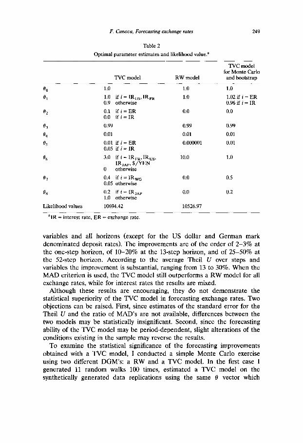
The results of the forecasting exercise are presented in table 1. The model (9)-(10) is estimated over the 1979.1-1985.52 sample and forecasts are generated from 1986.1 up to 1987.51. The 'optimal' 0 vector is presented in table 2, together with the maximized value of the likelihood and the value of the likelihood for the approximated RW model.

It is easy to see that the TVC model improves upon a RW model according to all criteria. When the Schwarz criterion is used the difference between the maximized values of the likelihood of the two models is significant. When the Theil U-statistic is used, the TVC model dominates a RW model for all

Table 1

Estimation sample 1979.1-1985.52/Forecasting sample 1986.1-1987.51.

Average Steps Average at steps over Overall

Variable 1 13 52 1 13 52 steps average

Theil U statistics $/DM 0.9724 0.7574 0.5096 0.9817 0.8726 0.8314 0.7187 $/L 0.9829 0.8172 0.7422 0.8738 $/SF 0.9780 0.7804 0.6379 0.7060 $/FF 0.9740 0.8295 0.5591 0.7697 YEN/$ 0.9758 0.8840 0.6890 0.7940 IRwG 0.9984 1.1182 1.9381 1.3418 IRuK 0.9851 0.7905 0.5743 0.7269 IRsw 0.9817 1.0569 0.6270 0.8647 IRFR 0.9890 0.8577 0.5744 0.7446 IRus 1.0130 1.1772 1.9680 1.4071 IRjAp 0.9479 0.5599 0.3309 0.4918

0.8581

Ratio of MAD's

$/DM 0.9427 0.7633 0.4050 1.0914 1.0244 0.8843 0.6650 $/L 0.7612 0.6885 0.3359 0.5694 $/SF 1.1812 1.1236 0.7358 0.9312 $/FF 1.0000 0.6822 0.6626 0.7823 YEN/$ 0.9885 0.8009 0.5889 0.7545 IRwG 1.0521 1.1967 2.0369 1.4436 IRuK 1.1436 2.4739 1.3888 1.9063 IRsw 0.4091 0.2572 0.1320 0.2161 IRFR 2.4501 1.5066 1.1875 1.4219 IRus 1.0224 1.1832 1.9335 1.3574 IRjAp 0.9605 0.5919 0.3209 0.4744

0.9555


Table 2

Optimal parameter est imates and likelihood value, a

249

TVC model for Monte Carlo

TVC model R W model and bootstrap

1.0 1.0 1.0

1.0 if i = I R u s , IRFR 1.0 1.02 if i = E R 0.9 otherwise 0.96 if i = IR

0.1 if i = E R 0.0 0.0 0.0 if i = IR

0.99 0.99 0.99

0.01 0.01 0.01

0.01 if i = E R 0.000001 0.01 0.05 if i = IR

3.0 if i = IRFR, I R u s , 10.0 1.0 IRjAp, S / Y E N

0 otherwise

0.4 if i = IRwG 0.0 0.5 0.05 otherwise

0.2 if i = IRjA P 0.0 0.2 1.0 otherwise

10694.42 10526.97

00 01

02

03 04 05

06

07

08

Likelihood values

a iR = interest rate, E R = exchange rate.

variables and all horizons (except for the US dollar and German mark denominated deposit rates). The improvements are of the order of 2-3% at the one-step horizon, of 10-20% at the 13-step horizon, and of 25-50% at the 52-step horizon. According to the average Theil U over steps and variables the improvement is substantial, ranging from 13 to 30%. When the MAD criterion is used, the TVC model still outperforms a RW model for all exchange rates, while for interest rates the results are mixed.

Although these results are encouraging, they do not demonstrate the statistical superiority of the TVC model in forecasting exchange rates. Two objections can be raised. First, since estimates of the standard error for the Theil U and the ratio of MAD's are not available, differences between the two models may be statistically insignificant. Second, since the forecasting ability of the TVC model may be period-dependent, slight alterations of the conditions existing in the sample may reverse the results.

To examine the statistical significance of the forecasting improvements obtained with a TVC model, I conducted a simple Monte Carlo exercise using two different DGM's: a RW and a TVC model. In the first case I generated 11 random walks 100 times, estimated a TVC model on the synthetically generated data replications using the same 0 vector which


produced table 1, and constructed the frequency distribution of the resulting Theil U and ratio of MAD statistics. To make the experiment credible, I imposed that the drift and the conditional variances of the simulated random walks must be the same as those of the five exchange rates and the six interest rates over the 1979.1-1987.51 period. In the second case, I generated 11 time series 100 times, using a TVC model and the parameters presented in the last column of table 2, and estimated a TVC model, using the 'optimal' # vector. The reason for estimating the model with a 0 vector which differs from the one used to generate the data is to check whether the forecasting ability of the model is independent of the exact choice of parameters.

Besides providing useful standard errors for the two statistics under a well-specified null hypothesis, these exercises may also tell us whether a naive rule (Theil U or ratio of MAD's greater than one) will give the correct rejection criterion with high probability.

Table 3 contains the mean value and the standard error (over replications) of the Theil U and of the ratio of MAD statistics at 1, 13, 52 steps and its standard error for each of the 11 variables of the system when the conditional variances are estimated using nonparametric methods as in Pagan and Ullah (1988). Table 4 contains the same statistics when the DGM is a TVC model. For each step and each statistic I also report in each table the probability that a value greater than one is observed. 8

The results indicate that when a RW is used as DGM, the mean Theil U over replications at each of the four horizons considered is greater than one in 9 out of the 11 cases. The standard errors tend to be large. However, the values presented in table 1 for the 1- and 13-steps-ahead fall in the lower 5% of the simulated distribution for four out of five exchange rates. The standard errors at the 52-step horizon are huge and the values reported in table 1 for this horizon are insignificantly different from one. For the ratio of MAD's the results are stronger. The mean value is always substantially above one and the standard errors are larger than in the case of the Theil U. However, the values presented in table 1 for this statistic for all five exchange rates at 1- and 13-steps horizon fall in the lower 5% of the simulated distribution. Again for the 52-step horizon, none of the entries of table 1 is significantly different from one. Finally, if one uses a naive rule of preferring a RW model when the Theil U (ratio of MAD's) is above one, one would reject the TVC model when a RW is the true DGM, on average, in about 78% (99%) of the cases. 9

SGiven the computational complexity of this exercise, I was forced to limit the size of the Monte Carlo to 100 draws only. On a mainframe VAX machine using RATS programs it took approximately five hours of CPU time to construct each table.

9I also computed forecasting statistics when the conditional variance of the DGM is estimated with a GARCH(1,1) model. The results, which are available on request, are similar to those reported in table 3. The only difference is that the standard errors for the two statistics are somewhat smaller.

A

F .o

"0

C~


~ ~ ~ ~ ~ ~ ~ ~ ~ ~ . . . . • : ~ . ,_,~ ~ s ~ e ~

~ e ~ ~ ~ r -~ ~ ~ "* " • . ~'~ ~ ~ ¢ q ¢ ~

~ ~ .~ ~ •

A A A A A A A A A A A

251

e , i . ,

Q e ~

• - o.)

A~a

. E . D . C . - - J

252

A

"2

F. C a n o v a , Forecas t ing exchange rates

io!o io! ° !o ~ ~ • . . ~ • . ~ . . s $ •

{5 {5 {:5

~ ~ ~ ~ ~ ~. ~ oo • ~ • • " " ¢5 {5

• ~ ~ ~ ~ ~. ~ ~ ~ ~ ~.

A A A A A A A A A A A

.=.

e~

.=.

e~

~8

¢3 ~'z

..-=~

"=¢4

A ~ 0

8


Table 5

Theil U-statistics; 100 replications over 1986.1-1987.52 sample; 90% confidence interval; L = lower bound, U = upper bound.

Steps Average at steps Average over Overall


$/DM L 0.982 0.677 0.486 0.966 0.772 0.667 0.618 U 0.995 0.716 0.531 0.974 0.826 0.857 0.733

$/L L 0.999 0.766 0.682 0.807 U 1.006 0.798 0.727 0.865

$/SF L 0.984 0.712 0.519 0.642 U 0.997 0.744 0.646 0.728

$/FF L 0.994 0.774 0.499 0.687 U 1.003 0.849 0.849 0.784

YEN/$ L 0.997 0.940 0.758 0.701 U 0.998 0.958 0.817 0.813

IRwG L 0.947 0.895 1.376 1.003 U 0.956 1.016 1.593 1.196

IRuK L 0.907 0.691 0.514 0.646 U 0.974 0.702 0.581 0.738

IRsw L 0.937 0.759 0.584 0.772 U 0.943 0.884 0.634 0.895

IRvR L 0.980 0.660 0.502 0.670 U 0.986 0.705 0.583 0.764

IRus L 1.002 0.962 1.125 1.120 U 1.011 0.996 1.246 1.196

IRjAp L 0.948 0.746 0.281 0.411 U 0.957 0.785 0.377 0.538

0.816 0.878

When the true DGM is a TVC model, both the Theil U and the ratio of MAD's have mean values below one and the value of one is in the upper 5% of the simulated distribution, except for the one-step-ahead for some interest rates. Note also the standard errors under this DGM are smaller than in the previous case and that, although the 0 are mispecified, the estimated model still captures the nonlinear dependence present in the mean of the DGM.

To examine the robustness of the results to changes in the forecasting environment I conducted several experiments. First, I computed replications of the forecasting statistics using a suboptimal 0 vector (listed in the last column of table 2) to forecast the eleven variables of the model in 100 replications of the sample 1986.1-1987.51. Replications are constructed using an algorithm which bootstraps the normalized recursive residuals of the TVC model. Table 5 presents a 90% confidence band for the ordered Theil U over replications and indicates that, even when the parameters of the prior are


arbitrarily chosen, the TVC model is superior to the RW model in forecasting all the variables at all horizons (except for the Eurodollar rate). While the performance of the TVC model in forecasting exchange rates at the one-step horizon is unimpressive, at longer horizons the 90% confidence band for the Theil U-statistic is still significant below one. 1°

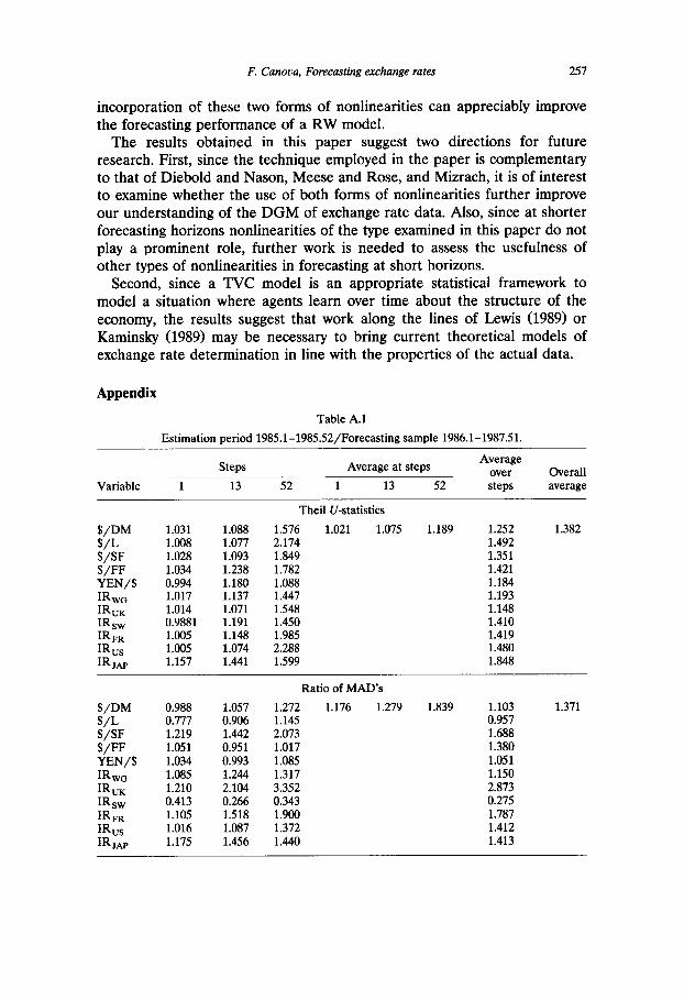
To further examine the robustness of the results to various alterations of the forecasting environment, first I sequentially reduced the estimation period dropping one year of data at a time and keeping the end date fixed at 1985.52. In this way one can check the extent to which the availability of data influences the forecasts of the TVC model. Second, I changed the forecasting sample. Engel and Hamilton (1990) have recently demonstrated that exchange rates exhibit long swings. Therefore, the forecasting performance of the model could be exaggerated if the forecasting sample coincides with one of these swings. To check for this possibility, I estimated the model from 1979.1 up to five different dates (1982.52-1983.26-1983.52-1984.26-1984.52) and then computed forecasting statistics for the following two years in each of the five cases. Table A.1 in the appendix provides the Theil U-statistic and the ratio of MAD's when the parameters of the TVC model are estimated with one year of data (1985.1-1985.52) and forecasts are computed over the 1986.1-1987.51 period. Table A.2 reports the forecasting statistics for the TVC model when the parameters are estimated over the 1979.1-1984.52 period and forecasts are computed over the 1985.1-1986.51 sample. H I find that the availability of data influences the MSE of the TVC model at all horizons and the performance of the model deteriorates when the forecasting sample is changed. However, even in these cases, the MSE and MAD of the TVC model are still smaller than those of the RW model for all the exchange rates considered.

Finally, to assess how sensitive the results are to changes in the model specification I conducted a few experiments by altering features of the prior. There are at least three features of the specification which can, in principle, account for the results o b t a i n e d - a seasonal prior mean, the presence of interest rates in the exchange rate equations, and the presence of nonlinearities. It is therefore worthwhile to try to disentangle the contribution of each of these features to the forecasting performance of the model. Table A.3 presents the forecasting statistics obtained when the prior means of the exchange rates are assumed to be random walks (i.e., 02 = 0 in all equations), while table A.4 presents the forecasting statistics when interest rates are

l°Since the results for Theil U and for the ratio of MAD's were qualitatively similar, I present results for the Theil U only. On a VAX mainframe, the exercise required about three hours of CPU time.

11I chose to present statistics for the 1985.1-1986.51 sample because the trend in all exchange rates in terms of the dollar changes during the sample. If the model exploited a local trend to forecast, it is bound to perform very poorly in this situation.


excluded from the exchange rate equations (i.e., 08 = 0 in all equations). The tables indicate that, although both a seasonal prior mean and the presence of interest rates in the exchange rate equations improve the general forecasting performance of the model, they are not primarily responsible for the substantial superiority of the TVC model over the RW model in the leng run. The 'good' long-run performance of the TVC model is therefore due the nonlinearities generated by time variation in the coefficients.

4.1. A comparison with the existing literature

It is not easy to compare the results of this paper with those presented in the existing literature for several reasons. First, the models recently employed by Diebold and Nason (1990), Meese and Rose (1989), and Mizrach (1990) are not nested in the framework of analysis of this paper. In their approach nonlinearities emerge in the functional specification of the DGM, i.e., their DGM is Yt =f(xt , [3), where f is nonlinear, while here the DGM is conditionally linear and nonlinearities appear because of time variation in the/3's. In addition, since they all estimate the coefficients of the model using a fixed window width, they do not allow for the type of time variation examined here. Second, in some cases the sampling frequency and the exchange rates used are not the same as ours. For example, Mizrach (1990) uses daily data from 1980 to 1985 on three EMS currencies (DM, FF, and Italian lira) in terms of the US dollar, while Engel and Hamilton (1990) use quarterly data for the 1973.1-1988.1 period for three currencies (DM, FF, L) in terms of the US dollar. Third, the samples used for estimation and forecasting are different from ours. This prevents, for example, a comparison with the work of Schinasi and Swamy (1989), who estimate a univariate frequentist version of the TVC model employed in this paper, using monthly data for the period 1973.1-1981.4, and forecast over the next 15 months. Fourth, some authors [e.g., Meese and Rose (1990) and Cheung and Pauly (1990)] examine only the in-sample fit of their model and provide no out- of-sample experiments.

The only meaningful comparison that can be made here is with the work of Diebold and Nason (1990). Diebold and Nason use weekly data for ten different currencies (Canadian dollar, FF, DM, Italian lira, YEN, SF, L, Belgium franc, Danish kroener, Dutch guilder) in terms of the US dollar for the period 1973.1-1987.38. Of this sample the first thirteen and a half years are used for estimation and about one year of data (1986.24-1987.38) is used to forecast from one to twelve weeks ahead. Table 6 presents the Theil U-statistic for the best nonparametric specification employed by Diebold and Nason and the Theil U of the TVC model when the parameters of the prior are chosen optimally over the period 1979.1-1986.23. For comparability, the Theil U-statistic for the TVC model is computed over the 1986.24-1987.38


Table 6

Comparison with Diebold and Nason (1990); estimation sample 1979.1-1986.38/forecasting sample 1986.39-1987.38; Theil U-statistics?

Steps Variable 1 4 12

$/DM TVC 0.9826 0.9289 0.8593 DN 0.9709 1.0128 1.0353

$/L TVC 0.9885 0.9307 0.8514 DN 0.9447 1.0610 0.9759

$/SF TVC 0.9923 0.9511 0.8778 DN 0.9939 1.0088 0.9853

$/FF TVC 0.9712 0.9085 0.8357 DN 1.0130 1.0473 1.0920

YEN/$ TVC 0.9895 0.9850 0.9797 DN 0.9271 1.0457 1.0116

aDN indicates the values of the statistics computed with the best model found by Diebold and Nason. For $/DM, $/FF, and $/SF, the best model required a value of 10 for the smoothing parameter, for $/L a smoothing parameter value of 0.2, and for YEN/$ a smoothing parameter value of 0.7. For all five currencies the best model has lag length of three.

period. One can see that the performance of the two specifications are approximately equivalent at the one-step horizon, but that the model of this paper substantially outperforms their best specification at the twelve-step horizon.

5. Conclusions

This paper shows that a TVC model produces complex nonlinear dependencies in the moments of generated time series, replicates features of the conditional and the unconditional distributions of actual exchange rates, and improves upon the point forecasts of a RW model. It also demonstrates that the improvements obtain at various forecasting horizons and persist when parameters are chosen arbitrarily and when the forecasts are computed over repeated samples.

Two ingredients of the methodology are primarily responsible for the results: the use of t ime variation in the coefficients, which produces a specific form of nonlinearity and nonnormality in the estimated process, and the use of a Bayesian 'shrinkage' procedure, which exploits common features of several exchange markets. Neither of these features was exploited in previous work. Time variation in the coefficients was not, in general, allowed in the estimation procedure. Nor were interdependences across markets explicitly modelled and accounted for in the estimation. The paper shows that the


incorporation of these two forms of nonlinearities can appreciably improve the forecasting performance of a RW model.

The results obtained in this paper suggest two directions for future research. First, since the technique employed in the paper is complementary to that of Diebold and Nason, Meese and Rose, and Mizrach, it is of interest to examine whether the use of both forms of nonlinearities further improve our understanding of the DGM of exchange rate data. Also, since at shorter forecasting horizons nonlinearities of the type examined in this paper do not play a prominent role, further work is needed to assess the usefulness of other types of nonlinearities in forecasting at short horizons.

Second, since a TVC model is an appropriate statistical framework to model a situation where agents learn over time about the structure of the economy, the results suggest that work along the lines of Lewis (1989) or Kaminsky (1989) may be necessary to bring current theoretical models of exchange rate determination in line with the properties of the actual data.

Appendix

Table A.1

Estimation period 1985.1-1985.52/Forecasting sample 1986.1-1987.51.



Theil U-statistics

$/DM 1.031 1.088 1.576 1.021 1.075 1.189 1.252 $/L 1.008 1.077 2.174 1.492 $/SF 1.028 1.093 1.849 1.351 $/FF 1.034 1.238 1.782 1.421 YEN/$ 0.994 1.180 1.088 1.184 IRwG 1.017 1.137 1.447 1.193 IRug 1.014 1.071 1.548 1.148 IRsw 0.9881 1.191 1.450 1.410 IRFR 1.005 1.148 1.985 1.419 IRus 1.005 1.074 2.288 1.480 IRjAp 1.157 1.441 1.599 1.848

1.382

Ratio of MAD's

$/DM 0.988 1.057 1.272 1.176 1.279 1.839 1.103 $ /L 0.777 0.906 1.145 0.957 $/SF 1.219 1.442 2.073 1.688 $/FF 1.051 0.951 1.017 1.380 YEN/$ 1.034 0.993 1.085 1.051 IRw6 1.085 1.244 1.317 1.150 IRuK 1.210 2.104 3.352 2.873 IRsw 0.413 0.266 0.343 0.275 IRFR 1.105 1.518 1.900 1.787 IRus 1.016 1.087 1.372 1.412 IRjA p 1.175 1.456 1.440 1.413

1.371


Table A.2

Estimation period 1979.1-1984.52/Forecasting period 1985.1-1986.52.

Variable

Average Steps Average at steps over

1 13 52 1 13 52 steps Overall average

TheilU-statistics

$ / D M 0.988 0.884 1.140 1.021 1.111 1.121 0.981 $ / L 0.990 1.058 1.402 1.206 $ /SF 0.999 1.036 1.383 1.152 $ / F F 0.988 0.999 1.315 1.122 YEN/$ 0.992 0.968 1.145 1.023 IRwG 1.044 1.164 1.400 1.179 IRuK 1.034 1.005 1.089 0.968 IRsw 0.996 0.966 0.935 0.897 IRFR 1.016 0.886 1.105 0.934 IRus 0.991 0.929 0.668 0.780 IRjA P 1.019 1.092 0.726 0.988

1.019

Ratio of MAD's

$ / D M 0.987 0.833 1.018 1.051 1.109 1.039 0.867 $ / L 0.891 0.700 0.595 0.677 $ /SF 0.973 0.861 0.887 0.920 $ / F F 0.950 1.003 1.152 1.048 YEN/$ 1.001 1.025 0.952 0.990 IRwG 1.091 1.346 1.522 1.361 IRuK 1.060 1.033 0.947 1.016 IRsw 1.001 1.021 0.865 0.972 IRFR 1.103 1.171 1.108 1.145 IRus 1.003 1.020 0.990 1.039 IRjA P 1.089 1.134 1.062 1.098

1.012

Table A.3

Estimation period 1979.1-1985.52/Forecasting sample 1986.1-1987.51; no seasonal prior mean.



Theil U-statistics

$ / D M 0.9643 0.7657 0.4778 0.9825 0.8757 0.8214 0.7105 $ / L 0.9762 0.8061 0.7395 0.8704 $ /SF 0.9711 0.8006 0.6177 0.7058 $ / F F 0.9753 0.8347 0.4982 0.7527 YEN/$ 0.9758 0.8404 0.6890 0.7940 IRwG 0.9984 1.1191 1.9431 1.3437 IRuK 0.9860 0.7927 0.5741 0.7269 IRsw 0.9854 1.0340 0.6223 0.8646 IR FR 0.9890 0.8522 0.5742 0.7446 IRus 1.0139 1.1809 1.9679 1.4071 IRjA P 0.9471 0.5640 0.3309 0.4918

0.8556


Table A.3 (continued)

259

Steps Average at steps

Variable 1 13 52 1 13 52

Average over steps

Overall average

Ratio of MAD's

$ /DM 0.9382 0.7698 0.3908 0 .9895 0.9206 0 . 8 1 6 5 0.6496 $ /L 0.7570 0.6853 0.3380 0.5694 $ /SF 1.1683 1 .1387 0.7256 0.9274 $ /FF 1.0000 0.6837 0.5939 0.7618 YEN/$ 0 . 9 8 8 5 0.8009 0.5889 0.7547 IRwo 1.0521 1 .1971 2.0437 1.4460 IRuK 1.1436 1 .4763 1.3881 1.2345 IRsw 0.4091 0.2572 0.1320 0.2165 IRFR 1.5440 1 .5018 1.1871 1.3446 IRus 1.0224 1 .1832 1.9335 1.3574 IRjA P 0.9605 0.5918 0.3209 0.4744

0.8851

Table A.4

Estimation sample 1979.1-1985.52/Forecasting sample 1986.1-1987.51; system with exchange rates only.



TheilU-statistics

$ /DM 0.9866 0.8063 0.4854 0.9906 0.8832 0 . 6 3 7 5 0.7095 $ / L 0.9984 1 .0000 0.8984 0.9483 $ /SF 0.9912 0.8397 0.6223 0.7951 $ /FF 0.9878 0.8857 0.4928 0.7697 YEN/$ 0.9794 0.8840 0.6886 0.7939

0.8033

Ratio of MAD's

$ /DM 0.9652 0.8346 0.4116 0.9910 0.8944 0.5537 0.6593 $ /L 0.7684 0.8769 0.4145 0.6286 $ /SF 1.2000 1 .2110 0.7297 0.9861 $ /FF 1.0361 0.7486 0.6243 0.7716 YEN/$ 0 . 9 8 8 5 0.8010 0.5885 0.7543

0.7599

References

Blattberg, R. and T. Sargent, 1971, Regression with nonstable Gaussian disturbances: Some sampling results, Econometrica 39, 501-510.

Boothe, P. and D. Glassman, 1987, The statistical distribution of exchange rates, Journal of International Economics 22, 297-319.

Canova, F., 1988, Seasonalities in foreign exchange markets, Working paper no. 8901 (Brown University, Providence, RI).

Canova, F., 1992, An alternative approach to modelling and forecasting seasonal time series, Journal of Business and Economic Statistics 10, 97-108.


Cheung, Y. and P. Pauly, 1990, Random coefficients autoregressive modelling of conditionally heteroskedastic processes: Short run exchange rate dynamics, Manuscript (University of Toronto, Toronto).

Clark, P., 1973, A subordinated stochastic process model with finite variance for speculative prices, Econometrica 41, 136-156.

Diebold, F., 1988, Empirical modelling of exchange rate dynamics (Springer Verlag, New York, NY).

Diebold, F. and J. Nason, 1990, Nonparametric exchange rate predictions?, Journal of Interna- tional Economics 28, 315-328.

Diebold, F. and M. Nerlove, 1989, The dynamic exchange rate volatility: A multivariate latent-factor ARCH model, Journal of Applied Econometrics 4, 1-22.

Doan, T., R. Litterman, and C. Sims, 1984, Forecasting and conditional projections using a realistic prior distribution, Econometric Reviews 3, 1-100.

Domowitz, I. and C. Hakkio, 1985, Conditional variance and the risk premium in foreign exchange markets, Journal of International Economics 19, 47-66.

Engel, C. and J. Hamilton, 1990, Long swings in the exchange rate: Are they in the data and do markets know it?, American Economic Review 80, 689-713.

Engle, R., D. Lilien, and R. Robins, 1987, Estimating time varying risk premia in the term structure: The ARCH-M model, Econometrica 55, 391-408.

Engle, R. and M. Watson, 1985, The Kalman filter: Application to forecasting and rational expectations models, in: T. Bewley, ed., Advances in econometrics, 5tb world congress, Vol. 1 (Cambridge University Press, Cambridge, MA) 245-283.

Fama, E., 1976, Foundations of finance (Basic Books, New York, NY). Fama, E. and R. Roll, 1968, Some properties of symmetric stable distributions, Journal of the

American Statistical Association 63, 817-836. Friedman, D. and S. Vandersteel, 1982, Short run fluctuations in foreign exchange rates:

Evidence from the data 1973-1979, Journal of International Economics 13, 171-186. Gallant, R., D. Hsieh, and G. Tauchen, 1990, On fitting a recalcitrant series: The pound/dollar

exchange rate, 1974-1983, in: W. Barnett, J. Powell, and G. Tauchen, eds., Nonparametric and semiparametric methods in econometrics and statistics, Proceedings of the 5th international symposium in economic theory and econometrics (Cambridge University Press, Cam- bridge, MA).

Geweke, J., 1989, Bayesian inference in econometric models using Monte Carlo integration, Econometrica 57, 1317-1340.

Granger, C. and A. Anderson, 1978, An introduction to bilinear time series models (Vandenhoeck and Ruprecht, G5ttingen).

Hamilton, J., 1989, A new approach to the economic analysis of nonstationary time series and the business cycles, Econometrica 57, 357-384.

Hsieh, D., 1988, The statistical properties of daily foreign exchange rates: 1974-1983, Journal of International Economics 24, 129-145.

Hsieh, D., 1989, Modelling heteroskedasticity in daily exchange rates, Journal of Business and Economic Statistics 7, 307-318.

Kaminsky, G., 1989, The peso problem and the behavior of the exchange rate: The dollar-pound exchange rate, 1976-1987, Manuscript (University of San Diego, San Diego, CA).

Koenker, R.W. and G.W. Basset, 1982, Tests of linear hypothesis and L - 1 estimation, Econometrica 50, 1577-1583.

Lewis, K., 1989, Can learning affect exchange rate behavior? The case of the dollar in the early 1980's, Journal of Monetary Economics 23, 79-100.

Lipster, R. and A. Shiryayev, 1978, Statistics of random processes (Springer Verlag, New York, NY).

Litterman, R., 1982, Specifying VAR's for macroeconomic forecasting, Staff report no. 92 (Federal Reserve of Minneapolis, Minneapolis, MN).


Ljung, L. and T. Soderstrom, 1987, Theory and practice of recursive identification (MIT Press, Cambridge, MA).

Meese, R. and K. Rogoff, 1983a, Empirical exchange rate models of the seventies: Do they fit out of sample, Journal of International Economics 14, 3-24.

Meese, R. and K. Rogoff, 1983b, The out-of-sample failure of empirical exchange rate models: Sampling error or misspecification, in: J. Frankel, ed., Exchange rate and international economics (University of Chicago Press, Chicago IL).

Meese, R. and A. Rose, 1989, An empirical assessment of non-linearities in model of exchange rate determination, Discussion paper no. 367 (Board of Governors of the Federal Reserve System, International Finance Division, Washington, DC).

Mizrach, B., 1990, Multivariate nearest neighbor forecasts of EMS exchange rates, Journal of Applied Econometrics, forthcoming.

Pagan, A. and A. Ullah, 1988, The econometric analysis of models with risk terms, Journal of Applied Econometrics 3, 87-105.

Pagan, A. and K. Yong, 1990, Nonparametric estimation and the risk premium, in: W. Barnett, J. Powell, and G. Tauchen, eds., Nonparametric and semiparametric methods in econometrics and statistics, Proceedings of the 5th international symposium in economic theory and econometrics (Cambridge University Press, Cambridge).

Rao, P., 1984, Nonparametric functional estimation (Academic Press, New York, NY). Rosenberg, B., 1973, Random coefficients models: The analysis of a cross section of time series

by stochastically convergent parameter regression, Annals of Economic and Social Measure- ment 2, 399-428.

Sarris, A., 1973, A Bayesian approach to estimation of time varying regression coefficients, Annals of Economic and Social Measurement 2, 501-523.

Schinasi, G. and P.A. Swamy, 1989, The out-of-sample forecasting performance of exchange rate models when coefficients are allowed to change, Journal of International Money and Finance 8, 375-390.

Schwarz, G., 1978, Estimating the dimension of a model, American Statistics 6, 461-464. Shafear, S. and al., 1975, Alternative models of systematic risk, in: E. Elton and M. Gruber, eds.,

International capital markets: An inter and intra country analysis (North-Holland, Amster- dam) 150-161.

Sims, C., 1984, On the martingale behavior of asset prices, Working paper no. 205 (University of Minnesota, Minneapolis, MN).

Sims, C., 1986, Bayesmth: A program for multivariate Bayesian interpolation, Working paper no. 234 (University of Minnesota, Minneapolis, MN).

Sims, C., 1989, A nine variable probabilistic macroeconomic forecasting model, Discussion paper no. 14 (Institute for Empirical Macroeconomics, Federal Reserve Bank of Minneapolis, Minneapolis, MN).

Thisted, R. and W. Wecker, 1981, Predicting a multitude of time series, Journal of the American Statistical Association 76, 516-523.

Tsay, R., 1987, ARCH and time varying parameter model, Journal of the American Statistical Association 82, 590-604.

Weiss, A., 1984, ARMA models With ARCH errors, Journal of Time Series Analysis 5, 129-143. Wolff, C., 1987, Time varying parameters and the out-of-sample forecasting performance of

structural exchange rate models, Journal of Business and Economic Statistics 5, 87-97. Zellner, A. and H.S. Hong, 1989, Forecasting international growth rates using Bayesian shrink-

age and other procedures, Journal of Econometrics 40, 183-202.

modelling and forecasting exchange rates with a bayesian time-varying coefficient model

Documents