modelling and control of the dynamical mechanical systems

Modelling and Control of the DynamicalMechanical Systems and Walking Robots

Sergej Celikovsky

Department of Control EngineeringFaculty of Electrical Engineering

Czech Technical University in Prague

and

Institute of Information Theory and AutomationCzech Academy of Sciences

Introduction Underactuated 2D-walking Modeling Virtual constraints Constraints realization Sensors Skipped Literature

Outline

1 Introduction and walking robots classification

2 Underactuated planar walking

3 Modeling of mechanical systems

4 Walking design using virtual holonomic constraints

5 Input-output exact feedback linearization and constraintsrealization

6 Remarks on sensors, estimation and identification

7 Related skipped problems

8 Literature

S. Celikovsky Modelling and Control of the Walking Robots 2 / 58


Walking robotsClassification of walking robots

Static walking:center of mass always above the feet, the robot can not fall, evenif stopped at any time.

Dynamic walking: center of mass not always above the feet, itshould go on moving not to fall

Two-dimensional walking (2D-walking):Only sagittal plane studied, the forward movement and stability isbelieved to be the crucial for the walking-like movement.

Three-dimensional walking (3D-walking):Full orientation including the lateral movement studied, the lateralbalance should be (even intuitively) easier to handle, than theforward movement.



Walking robotsClassification of walking robots

Fully actuated walking robots:

Large feet in full contact with the ground and actuated ankles.

Stable (static) walking usually fully actuated.

Unstable (dynamic) walking can be also fully actuated.

Zero moment point (ZMP) should be computed and ensuredto be bellow the feet.

Underactuated walking robots:

Unstable (dynamic) walking only.

Underactuated angle is at the pivot point.

Feet are absent or very small with weakly actuated ankles.



Walking robotsFully actuated walking

Slow movement, weak coupling between links and strongactuators - the kinematic trajectory planning possible andimplementable through the standard control engineeringdesign (e.g. PD or PID controllers). ZMP condidion imposeactuators limitations.

Fully actuated mechanical system is theoretically wellunderstood even if its full dynamics (including forces andtorques) should be considered - computed torque principle.

The typical fully actuated static walking humanoids (likeHONDA) are heavy, with strong joints actuation and veryslow dynamic walking coupling between the links dynamics, oreven with the static walking only.



Walking robot with knees, ankles, feet and torsoFully actuated state - ZMP bellow the foot



Walking robotsIntrinsic walking is the underactuated walking

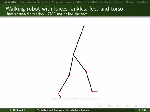
BUT! What if the walk should be swift, legs light, energyefficiency strived for? Then the fully actuated walkingrobotics is not an option.

The ZMP condition is demanding and therefore the torque inankles should be, anyway, small, only the balancing one andto facilitate the full foot contact with the ground.

If the ZMP condition is violated, the full flat contact of thefoot is lost and another angle - another degree of freedomappears - yet, there is unactuated angle again and the wholerobot becomes underactuated.



Walking robot with knees, ankles, feet and torsoUnderactuated situation - ZMP not bellow the foot



Walking robotsIntrinsic walking is the underactuated walking

Real walking: both the fully actuated and the underactuatedwalking phases present.

Conclusion: It is reasonable to study the underactuatedwalking, as a natural abstraction of weak ankles up to thecase with NO ankles.



Walking robotsPlanar walking



Walking robots

Plan: The underactuated planar walking will be further studiedin detail.

Indeed, as noted before, the control along the sagittal plane is themost challenging and interesting one. Instability is actually thesource of the movement forward.



Underactuated mechanical systemsIntroduction

Less actuators than degrees offreedom (DOF]

The n-link with n − 1 actuators

Nonlinear techniques needed

Pendubot

Acrobot

Rotational inverted pendulum

...

x

y



Underactuated mechanical systemsAcrobot (aka Compass-Gait Walker (CGW))

The simplest underactuatedwalking model, 2 DOF, 1actuator.

To model walking, theunderactuated angle is at thepivot point.

“Planar” walking-like movementpossible only theoretically.

Acrobot, or Compass-GaitWalker (CGW), ...

x

y

q1

q2

τ2



Underactuated mechanical systemsThe four-link walker

Acrobot walking: unrealistic

4-link: more realistic

4-link: 4 DOF, 3 actuators

Legs with knees, without feet

x

y

q1

q2

−q3

q4

τ2

τ3

τ4



Underactuated mechanical systemsThe four-link walker - Configuration and physical parameters

x

y

q1

q2

−q3

q4

u2

u3

u4

m1

lc1

l1

m2

lc2

l2 m3

lc3l3

m4

lc4

l4

m1,m4 1 [Kg] m2,m3 1.5 [Kg]l1, l4 0.5 [m] lc1, lc4 0.3 [m]l2, l3 0.6 [m] lc2, lc3 0.4 [m]



Underactuated mechanical systemsThe three-link (aka Compass-Gait Walker with Torso)

l3

lc3

q1

q3

q2l1

lc1

l2

lc2

m1m2

m3

stanceleg swing

leg

torso



Underactuated mechanical systemsPossible general underactuated planar n-link walker scheme

x

y

q1

q2

-q3

q4

τ5, τ2

τ3

τ4

-q5

qn

τn

qn-2

τn-2

qn-1τn-1



Modeling of the walking robotsTwo different model phases

1. Continuous-time phase (aka single support phase, ...). Model:ordinary differential equations with control inputs, resulting in thestandard controlled continuous-time system studied in varioussubjects before (B3B35ARI, B3M35NES, B3M35LSY).

2. Discrete-time phase (aka double-support phase). Model:uncontrolled mappings of the state to the new state, with somejump, or also impulsive system. It is a single application of adiscrete-time system without input.



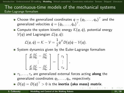
The continuous-time models of the mechanical systemsEuler-Lagrange formalism

Choose the generalized coordinates q = (q1, . . . , qn)> and thegeneralized velocities q = (q1, . . . , qn)>.

Compute the system kinetic energy K(q, q), potential energyV(q) and Lagrangian L(q, q):

L(q, q) = K − V =1

2qTD(q)q − V(q).

System dynamics given by the Euler-Lagrange formalismddt

∂L∂q1− ∂L

∂q1...

ddt

∂L∂qn− ∂L

∂qn

=

τ1...τn

,τ1, . . . , τn are generalized external forces acting along thegeneralized coordinates q1, . . . , qn, respectively.

D(q) = D(q)> > 0 is the inertia (aka mass) matrix.



The continuous-time models of the mechanical systemsEuler-Lagrange formalism

The Euler-Lagrange formalism gives the system of thesecond-order ordinary differential equations

D(q)q+C (q, q)q+G (q) = (τ1, . . . , τn)>, G (q) = −[∂V∂q

]>,

C (q, q)q =

[n∑

i=1

∂D(q)

∂qiqi

]q −

[∂

∂q

[1

2qTD(q)q

]]>,

C (q, q) is the matrix of the Coriolis and centrifugal forces,G (q) is the gravity vector.

The choices of generalized coordinates and generalizedvelocities are related:

∑ni=1 τidqi should be the infinitesimal

increment of energy of the system done by work of externalforces. In particular, if generalized coordinates are angles,then the generalized forces are torques.



The continuous-time models of the mechanical systemsFully actuated controlled system in standard form of the first-order ODE

Controlled inputs (actuators) are the generalized forces, all ofthem available and independent - full actuation:

u =

u1...un

=

τ1...τn

The state vector is x = (x1, . . . , x2n)> = (x1, x2)>

x1 = (q1, . . . , qn), x2 = (q1, . . . , qn).

The standard form of the first-order controlled system:

x = f ST (x) + GST (x)u, GST (x) = D(x1)−1

f ST (x) =(x2, f (x)

)>, f (x) = D−1(x1)

(−C (x1, x2)x2 − G (x1)

)>S. Celikovsky Modelling and Control of the Walking Robots 21 / 58


The continuous-time models of the mechanical systemsExact feedback feedback linearization and computed torque principle (inverse dynamics)

For fully actuated system take the feedback (introduce the new“virtual” input u)

u = f (x) + GST (x)u, u = [GST (x)]−1(u − f (x)),

which gives the simple linear system of n double integrators

x1 = xn+1, . . . , xn = x2n, xn+1 = u1, . . . , x2n = un.

This gives the simple model based implementation of any smoothkinematically planned trajectory qr (t), containing some PDcontroller (but any gains kpi < 0, kdi < 0, i = 1, . . . , n, sufficient):

u = [GST (x)]−1

qr1 + kp1 (q1 − qr1) + kd1 (q1 − qr1)

...qrn + kpn (qn − qrn) + kdn (qn − qrn)

− f (x)

.




Indeed, for virtual input u that is equivalent to

u =

qr1 + kp1 (q1 − qr1) + kd1 (q1 − qr1)...

qrn + kpn (qn − qrn) + kdn (qn − qrn)

Recalling, that x1 = (q1, . . . , qn), x2 = (q1, . . . , qn),x1 = xn+1, . . . , xn = x2n, xn+1 = u1, . . . , x2n = un and introducing

e1 = q1 − qr1, . . . , en = qn − qrn

givese1 = en+1, . . . , en = e2n,

en+1 = kp1 e1 + kd1 en+1, . . . , e2n = kpn en + kdn e2n.




Recall, that GST (x) = D(x1)−1, [GST (x)]−1 = D(x1) = D(q)giving

[GST (x)]−1f (x) = C (q, q)q + G (q)

u = D(q)

qr1 + kp1 (q1 − qr1) + kd1 (q1 − qr1)...

qrn + kpn (qn − qrn) + kdn (qn − qrn)

+C (q, q)q+G (q).

COMPUTED TORQUE PRINCIPLE (CTP): substituting thedesired linear second order dynamics of q into the second orderODE obtained by Euler-Lagrange formalism gives the torque.

CTP introduced in robotics earlier than the exact feedbacklinearization (EFL) in nonlinear control theory.

Clearly, for the fully actuated mechanical systems EFL=CTP.



The continuous-time models of the mechanical systemsUnderactuated mechanical systems

Underactuated system dynamics given by the Euler-Lagrangeformalism

ddt

∂L∂q1− ∂L

∂q1

...ddt

∂L∂qn− ∂L

∂qn

=

τ1...τn

, τ1 = · · · = τk = 0.

Coordinates q1, . . . , qk directly unactuated, qk+1, . . . , qndirectly actuated, k is the underactuation degree.

Analogously, as for the fully actuated systems (D,C ,G thesame), the second order dynamics obtained.

D(q)q + C (q, q)q + G (q) = (0, . . . , 0, τk+1, . . . , τn)>



The continuous-time models of the mechanical systemsUnderactuated controlled system in standard form of the first-order ODE

u =

0...0

uk+1...un

=

0...0

τk+1...τn

, x = (x1, . . . , x2n)> = (x1, x2)>

x1 = (q1, . . . , qn), x2 = (q1, . . . , qn).

x = f ST (x) + GST (x)u, GST (x) = D(x1)−1

f ST (x) =(x2, f (x)

)>, f (x) = D−1(x1)

(−C (x1, x2)x2 − D(x1)

)>Exact feedback linearization and computed torque principle clearlynot possible using the previously described approach.



The continuous-time models of the mechanical systemsUnderactuated mechanical planar walking-like chains

2D-walking models have usually underactuation degree k = 1.The angle at the pivot point q1 is unactuated, q2, . . . , qndirectly actuated.

For these planar walking-like chains, kinetic energy does notdepend on q1, i.e. D(q) ≡ D(q2, q3, . . . , qn) and q1 is calledcyclic variable, q2, . . . , qn are called shape variables. Anyabsolute orientation angle is also cyclic variable. Relativeangles are shape variables.

3D-walking models have underactuation degree k = 2, butonly one cylic variable.



The continuous-time models of the mechanical systemsUnderactuated mechanical planar walking-like chains

Summarizing, the underactuated planar walking models areas follows:

D(q)q + C (q, q)q + G (q) =

0u2...un

But, how to obtain these models in detail?



The continuous-time models of the mechanical systemsEuler-Lagrange formalism for planar mechanical chains - computing the K and V

Lagrangian L requires kinetic and potential energy

L(q, q) = K − V =1

2qTD(q)q − V(q).

The kinetic energy K of the each rigid link:

K =1

2mvTv +

1

2ωTIω.

Here, m is the total mass of the each rigid link; v is the link center

of mass (COM) velocity vector, ω is the link rotation angular

velocity with respect to its COM; I is the symmetric 3 × 3 inertia

tensor of the link. In 2D case, just a scalar.The potential energy V of the each rigid link: V = mgh. Here,

h is the height of the center of mass of the link.Choice of q, q depends on available inputs. This causes oftencomplex D(q).



The continuous-time models of the mechanical systemsEuler-Lagrange formalism for planar mechanical chains - Acrobot (aka CGW) example.

q1

q2

l1

lc1

l2

lc2

m1

m2




x

ybase frame

m1

m2

q1

−q2lc1

l1

lc2l2

link #1

link #2




K =1

2qTD(q)q, D(q) =

[θ1 + θ2 + 2θ3 cos q2 θ2 + θ3 cos q2

θ2 + θ3 cos q2 θ2

]

C (q, q) =

[−q2θ3 sin q2 −(q1 + q2)θ3 sin q2

q1θ3 sin q2 0

]V(q) = [θ4 cos q1 + θ5 cos (q1 + q2)]

G (q) =

[−θ4 sin q1 − θ5 sin (q1 + q2)

−θ5 sin (q1 + q2)

],

θ1 = m1l2c1 + m2l

21 + I1, θ2 = m2l

2c2 + I2,

θ3 = m2l1lc2, θ4 = gm1lc1 + gm2l1, θ5 = gm2lc2.



The continuous-time models of the mechanical systemsThe three-link (aka Compass-Gait Walker with Torso)

l3

lc3

q1

q3

q2l1

lc1

l2

lc2

m1m2

m3

stanceleg swing

leg

torso



The continuous-time models of the mechanical systemsThe three-link (aka Compass-Gait Walker with Torso)

Mathematical model

D = [dij ], i , j = 1, 2, 3, D> = D > 0, G = [G1,G2,G3]>,

d11 = I1 + I2 + I3 + l21m2 + l21m3 + l2c1m1+

l2c2m2 + l2c3m3 + 2l1lc2m2 cos q2 + 2l1lc3m3 cos q3,

d12(q2) = m2l2c2 + l1m2 cos q2lc2 + I2

d13(q3) = m3l2c3 + l1m3 cos q3lc3 + I3, d23 = 0,

d22(q2, q3) = m2l2c2 + I2, d33(q2, q3) = m3l

2c3 + I3,

G1 = −g (l1m2 sin q1 + l1m3 sin q1 + lc1m1 sin q1+

lc2m2 sin q1 + q2 + lc3m3 sin q1 + q3) ,

G2 = −glc2m2 sin q1 + q2, G3 = −glc3m3 sin q1 + q3.



The continuous-time models of the mechanical systemsThe four-link model

x

y

q1

q2

−q3

q4

u2

u3

u4

m1

lc1

l1

m2

lc2

l2 m3

lc3l3

m4

lc4

l4

m1,m4 1 [Kg] m2,m3 1.5 [Kg]l1, l4 0.5 [m] lc1, lc4 0.3 [m]l2, l3 0.6 [m] lc2, lc3 0.4 [m]



The continuous-time models of the mechanical systemsThe four-link model

D(q)=

d11 d12 d13 d14

d21 d22 d23 d24

d31 d32 d33 d34

d41 d42 d43 d44

,C (q, q)=

C 1

C 2

C 3

C 4

,G (q)=

G1

G2

G3

G4

,d11 = (I1 + I2 + I3 + I4 + l21m2 + l21m3 + l21m4

+ l22m3 + l22m4 + l23m4 + l2c1m1

+ l2c2m2 + l2c3m3 + l2c4m4 − 2l1l3m4 cos(q2 + q3)

− 2l1lc3m3 cos(q2 + q3)− 2l2lc4m4 cos(q2 + q4)

+ 2l1l2m3 sin(q3) + 2l1l2m4 sin(q3) + 2l2l3m4 sin(q2) + 2l1lc2m2 sin(q3)

+ 2l2lc3m3 sin(q2) + 2l3lc4m4 sin(q4)− 2l1lc4m4 sin(q2 + q3 + q4))

d12 = (I3 + I4 + l23m4 + l2c3m3 + l2c4m4

− l1l3m4 cos(q2 + q3)− l1lc3m3 cos(q2 + q3)

− l2lc4m4 cos(q2 + q4) + l2l3m4 sin(q2) + l2lc3m3 sin(q2)

+ 2l3lc4m4 sin(q4)− l1lc4m4 sin(q2 + q3 + q4))



The continuous-time models of the mechanical systemsFour-link model

d13 = (I2 + I3 + I4 + l22m3 + l22m4 + l23m4 + l2c2m2 + l2c3m3 + l2c4m4−l1l3m4 cos(q2 + q3)− l1lc3m3 cos(q2 + q3)− 2l2lc4m4 cos(q2 + q4)+l1l2m3 sin(q3) + l1l2m4 sin(q3) + 2l2l3m4 sin(q2) + l1lc2m2 sin(q3)+2l2lc3m3 sin(q2) + 2l3lc4m4 sin(q4)− l1lc4m4 sin(q2 + q3 + q4))

d14 = (I4 + l2c4m4 − l2lc4m4 cos(q2 + q4)+l3lc4m4 sin(q4)− l1lc4m4 sin(q2 + q3 + q4))

d22 = (m4l23 + 2m4 sin(q4)l3lc4 + m3l2c3 + m4l2c4 + I3 + I4)

d23 = (m4l23 + 2m4 sin(q4)l3lc4 + l2m4 sin(q2)l3 + m3l2c3 + l2m3 sin(q2)lc3+m4l2c4 − l2m4 cos(q2 + q4)lc4 + I3 + I4)

d24 = (m4l2c4 + l3m4 sin(q4)lc4 + I4)

d33 = (I2 + I3 + I4 + l22m3 + l22m4 + l23m4+l2c2m2 + l2c3m3 + l2c4m4 − 2l2lc4m4 cos(q2 + q4) + 2l2l3m4 sin(q2)+2l2lc3m3 sin(q2) + 2l3lc4m4 sin(q4))

d34 = (I4 + l2c4m4 − l2lc4m4 cos(q2 + q4) + l3lc4m4 sin(q4))

d44 = (m4l2c4 + I4)



The continuous-time models of the mechanical systemsFour-link model

G1 = −glc4m4 sin(q1 + q2 + q3 + q4)− gl2m3 sin(q1 + q3)− gl2m4 sin(q1 + q3)−glc2m2 sin(q1 + q3)− gl1m2 sin(q1)− gl1m3 sin(q1)− gl1m4 sin(q1)−glc1m1 sin(q1)− gl3m4 sin(q1 + q2 + q3)− glc3m3 sin(q1 + q2 + q3)

G2 = −glc4m4 sin(q1 + q2 + q3 + q4)− gl3m4 sin(q1 + q2 + q3)−glc3m3 sin(q1 + q2 + q3)

G3 = −glc4m4 sin(q1 + q2 + q3 + q4)− gl2m3 sin(q1 + q3)−gl2m4 sin(q1 + q3)− glc2m2 sin(q1 + q3)−gl3m4 sin(q1 + q2 + q3)− glc3m3 sin(q1 + q2 + q3)

G4 = −glc4m4 sin(q1 + q2 + q3 + q4).



The hybrid models of the mechanical systemsSwing and impact phases

Contact mechanical systems are modeled using bothcontinuous-time and discrete-time dynamics.

Hybrid systems combine both dynamics:

continuous-time dynamics

x = F (x , u), x ∈ C

discrete-time dynamics.

x+ = Γ(x−, u), x ∈ D

Usually, D is some lower dimensional submanifold of C.

For walking Γ(x−, u) ≡ Γ(x−), as only impulsive forces acting.



The hybrid models of the mechanical systemsSwing and impact phases

Actually: q+ = Φ(q−)q− and q+ undergoes some simplerelabeling map due to switching the legs. Φ is called as theimpact matrix.

Switching of legs is to keep the same continuous time modelfor both legs being the swing one. Alternative would be hybridsystems with two continuous-time models.

Both leg are usually assumed to have the same properties.



Discrete-time dynamics modelingImpact matrix modeling

When the swing leg of the Acrobot hits the ground, theimpact occurs.

Impact causes instantaneous jump in angular velocities qwhile angular positions q remain continuous in time.

The impact is modeled as a contact between two rigid bodies:

double support phase is instantaneous,overall energy and momentum is preserved,no swing leg rebound,no swing leg slipping.

The impact modeling is based on the continuous-time modelsshortly “just before the impact” and “just after the impact”.



Discrete-time dynamics modelingImpact matrix modeling

The extended continuous-time model is needed that unifiesboth situations. It has more DOF generalized coordinatesdenoted qe , its matrix of inertia denoted De(qe).

The impact matrix computation is based on the equations:

De

[q+e − q−e

]= Fext , E2(q−e )q+

e = 0,

where E2(q−e ) = ∂Υ(qe )

∂qe(q−

e ), Υ represents swing leg’s end point

Carthesian coordinates, q−e corresponds to the double support

configuration. Vector Fext is the assumed cumulative effect of the

impulsive forces during the infinitesimally small time interval.

Fext is unknown, but can it be eliminated.E.g., for Acrobot there are 10 scalar variables: q−

e , q+e ,Fext and 6

equations. So, one can obtain 4 linear equations relating q−e and q+

e , i.e.,

consequently, two linear equations for q−, q+ in the form q+ = Φ(q−)q−.



Discrete-time dynamics modelingRelabeling map

At impact, the swing leg, respectively stance leg, becomes thenew stance leg, respectively the new swing leg.

Example: the Acrobot’s relabeling of q1 and q2 coordinates.

q2 q2

-q1 q1

This picture also helps to undestand the essence and the needof that previously mentioned extended model.



Virtual holonomic constraintsDefinition and regularity

Virtual holonomic constraints (VHC) of q ∈ Rn are equalities

ϕ1(q) = ϕ2(q) = . . . = ϕl(q) = 0.

Smooth functions ϕ1, . . . , ϕl satisfy rank{dϕ1(q), . . . ,dϕl(q)} = l∀q ∈ {q ∈ Rn|ϕ1(q) = · · · = ϕl(q) = 0}.

VHC are called global if ϕ1(q), . . . , ϕl(q) can be completed to aglobal diffeomorphism of Rn.

Locally regular VHC around some q0:

rank

∂ϕ1∂q...

∂ϕl∂q

(q0)D−1(q0)

[0k×nIn−k

]= l

Locally regular VHC: locally regular around any q0 ∈ Rn.



Walking design using virtual constraintsEXAMPLE: VHC for the four-link walking

Virtual holonomic constraints enforced by suitable feedback control

Number of DOF and actuators reduced, problem decomposed

Two different options:

I. Three constraining functions

Knees and hip angles made to depend on the stance leg angle

Design of 3 constraining functions

Constrained dynamics has 1 DOF and no actuator =uncontrolled generalized inverted pendulum

Cyclic property of unactuated variable lost

Example of the so-called noncollocated constraints



Walking design using virtual constraintsFour-link with 3 VHC - problem of stable tracking of the walking trajectory

Stable tracking of the above trajectory during swing phaseonly is not possible

Reason: generalized inverted pendulum is unstable.

generalized inverted pendulum = zero dynamics wrt. outputsϕ1 = q2 − Φ2(q1), ϕ2 = q3 − Φ3(q1), ϕ3 = q4 − Φ4(q1).

Nevertheless, one can design it to be hybrid stable, i.e.including impacts and multi-step walking.

Ch. Chevallereau, J. Grizzle and others: hybrid zero dynamics,hybrid minimum phase systems.

Physically: impact may have stabilizing influence. Intuitively,COM pointing downwards.

Analysis and proof very complicated, hybrid limit cycles,Poincare sections, ...



Walking design using virtual constraintsVirtual constraints for the four-link walking

II. Two constraining functions

both knees made to depend on the hip angle

design of 2 constraining functions

constrained dynamics has 2 DOF and 1 actuator

previously developed techniques for the Acrobot applicable

constrained dynamics easier enforced - the so-calledcollocated VHC (Celikovsky 2015, Celikovsky and Anderle2016–2017, Anderle and Celikovsky 2018.).



Realization of the virtual holonomic constraintsRegular VHC and input-output exact feedback linearization

x = f (x)+u1g1(x)+. . .+umg

m(x), y = [h1(x), . . . , hp(x)], m ≥ p,

x ∈ Rn, y ∈ Rp, u ∈ Rm, f (x0) = 0, rank[g1| · · · |gm](x0) = m, h(x0 = 0.

Lie derivative:

Lf h := f1∂h

∂x1+. . .+fn

∂h

∂xn, L0

f h := h, Lk+1f h := Lf L

kf h,∀k = 1, 2 . . .

Vector relative degree (r1, . . . , rp) :

Lg iLkf hj ≡ 0, ∀k = 0, . . . , rj − 2, i = 1, . . . ,m, j = 1, . . . , p and

rankD(x0) = p, D(x) :=

Lg1Lr1−1f h1 . . . LgmLr1−1

f h1...

...

Lg1Lrp−1f hp . . . LgmL

rp−1f hp

(x)

D is called as the decoupling matrix.




It holds (here (·)(r) stands for the r -th order time derivative): y(r1)1 (t)

...

y(rp)p (t)

= D(x)

u1...um

+

Lr1f h1...

Lrpf hp

.Moreover, there are r1 + r2 + . . .+ rn independent functions:

y1 = h1(x), y(1)1 = Lf h1(x), . . . , y

(r1−1)1 = Lr1−1

f h1(x), . . .

yp = hp(x), y(1)2 = Lf hp(x), . . . , y

(rp−1)p = L

rp−1f hp(x).

These function can be used as a part of new coordinates, giving(r1 + r2 + . . .+ rn)-dimensional linear subsystem, consisting from lindependent integrators chains having lengths r1, . . . , rp.




Note that:

D(x) =∂

∂u

y1(t)...

yl(t)

In other words, regular VHC are such that the mechanical systemwith n − k inputs un−k+1, . . . un and l outputs

y1 = ϕ1(q), y2 = ϕ2(q), . . . , yl = ϕl(q)

has the vector relative degree (2, . . . , 2).Therefore, the assumption l ≤ n− k is needed. One can enforce atmost as much constraints as it is the number of inputs.



Realization of the virtual holonomic constraintsRegular VHCs and input-output exact feedback linearization

Realization can be done e.g. by

y1 = −k11y1 − k2

1 y1, . . . , yl = −k1l yl − k2

l yl ,

where all k ’s are positive reals. Recall, thaty1 = ϕ1(q), y2 = ϕ2(q), . . . , yl = ϕl(q) and therefore also

y1 =∂ϕ1

∂qq, . . . , yl =

∂ϕl

∂qq.

x := (q>, q>)>, f (x) = (x1, . . . , xn,−D−1(Cq−G )>)>, G = D−1, y1...yl

= D(q, q)u+

L2f ϕ1...

L2f ϕl

=⇒ u = [D(q, q)]−1

y1 − L2f ϕ1

...yl − L2

f ϕl



Sensors, estimation and identificationSensors

All previous approaches to be implemented require stateestimation, or direct measurements of all states.

Angular positions measurement at rotary joints efficient andalmost noisy free.

Relative measurements: only increments of angle relative totheir initial value measured, e.g. IRC (Incremental RotaryenCoder) - usually optical, very good precision and low noise.

Absolute measurements: absolute angle, e.g. potentiometer(simple, cheap, but low precision), magnetic position sensor(Hall effect sensor, much better, but not as IRC), ...

Angle not related to any rotary joint, e.g. the angle at thepivot point (or any other absolute orientation angle),measured indirectly only, if the robot is autonomous:inertial sensors, digital gyroscopes, laser distance sensors...



Sensors, estimation and identificationState estimation

Velocities either measured directly by gyroscopes, orestimated.

For noisy-free angular positions measurements (e.g. IRC),numerical time derivative applicable, or filtered numerical timederivatives, fast evaluation circuit needed.

For the absolute orientation angle estimation morecomplicated.

In 2D-walking platforms often noisy-free measurement of theabsolute orientation angle implemented in supportingplatform.

Kalman filtering and other methods from control courses usedas well, with some adaptation (Extended Kalman Filter,Hybrid Kalman Filter, ...).



Sensors, estimation and identificationIdentification

Mechanical parameters can be well-measured in advance(weights, lengths, moments of inertia).

These measurements may serve for further tuning as theparameters initial estimates.

Noise in drives effects need to be attenuated.

If all angles are well measured, angular velocities and angularaccelerations well computed, estimation of θ1, θ2, ... becomesa standard linear problem, e.g. least squares and maximallikehood method applicable.

Again, there is a problem with absolute orientation angle. Butit can be handled easier, than in state estimation problem, asfor identification off-line experiments possible, using someframes and platforms with extra measurements,...



Sensors, estimation and identificationIdentification - Acrobot (aka CGW) example

D(q)q + C (q, q)q + G (q) =

[0u2

]

C (q, q) =

[−q2θ3 sin q2 −(q1 + q2)θ3 sin q2

q1θ3 sin q2 0

]

G (q) =

[−θ4 sin q1 − θ5 sin (q1 + q2)

−θ5 sin (q1 + q2)

],

θ1 = m1l2c1 + m2l

21 + I1, θ2 = m2l

2c2 + I2,

θ3 = m2l1lc2, θ4 = gm1lc1 + gm2l1, θ5 = gm2lc2.



Related skipped problems

Running robots

Jumping robots

And many others ...

Note, that running and jumping may be in a certain sense easierthan walking (compare to track and field athletes experience!)

Mathematical modeling explanation: no need for the complexcontinuous-time walking-like dynamics, with no contact withground, robot is governed just by laws of passive free movementunder the gravity and air resistance influence.



Literature

Ch. Chevallereau, G. Abba, Y. Aoustin, F. Plestan, E. R.Westervelt, C. Canudas-De-Wit, and J. W. Grizzle. Rabbit: atestbed for advanced control theory. IEEE Control Systems, 23 (5),57–79, 2003.

E. R. Westervelt and J. W. Grizzle and Ch. Chevallereau and J. H.Choi and B. Morris: Feedback Control of Dynamic Bipedal RobotLocomotion, CRC Press, 2007.

Ch. Chevallereau, G. Bessonnet, G. Abba, and Y. Aoustin. BipedalRobots: Modeling, Design and Walking Synthesis. Wiley-ISTE,2009.

J.W. Grizzle, C. Chevalereau, R.W. Sinnet, and A.D. Ames.Models, feedback control and open problems of 3D bipedal roboticwalking. Automatica, 50 (8), 1955–1988, 2014.

Surbhi Gupta and Amod Kumar. A brief review of dynamics andcontrol of underactuated biped robots. Advanced Robotics, 31 (12),607–623, 2017.



Selected publications

S. Celikovsky: Flatness and realization of virtual holonomic constraints inLagrangian systems, IFAC-PapersOnLine, Vol. 48, pp. 25-30, The 5th IFACWorkshop on Lagrangian and Hamiltonian Methods for Non Linear Control,(2015), Lyon, FR.

S. Celikovsky and M. Anderle: On the collocated virtual holonomic constraintsin Lagrangian systems, Proceedings of the American Control Conference, 2016,p. 6030-6035, Boston, US.

S. Celikovsky and M. Anderle: Hybrid invariance of the collocated virtualholonomic constraints and its application in underactuated walking ,IFAC-PapersOnLine. Volume 49, Issue 18, p. 802-807, The 10th IFACSymposium on Nonlinear Control Systems, Monterey, California, USA (2016).

K. Dolinsky and S. Celikovsky: Application of the Method of MaximumLikelihood to Identification of Biped Walking Robots. IEEE Trans. on ControlSystems Technology, vol. 26, 4 (2018), pp. 1500-1507.

S. Celikovsky and M. Anderle: Collocated Virtual Holonomic Constraints inHamiltonian Formalism and Their Application in the Underactuated Walking. InProceedings of the 11th Asian Control Conference (ASCC) 2017, pages192–197, Gold Coast, Australia, 2017.

M. Anderle and S. Celikovsky: On the Hamiltonian approach to the collocatedvirtual holonomic constraints in the underactuated mechanical systems. InLecture Notes in Electrical Engineering, volume 465, pages 554–568, 2018.


modelling and control of the dynamical mechanical systems

Documents