modelling, analysis and numerical simulations of
TRANSCRIPT
DEPARTMENT OF MATHEMATICS
FACULTY OF SCIENCE
UNIVERSITY OF ZAGREB
Ana Zgaljic Keko
Modelling, Analysis and Numerical Simulations of
Immiscible Compressible Two-phase Fluid Flow in
Heterogeneous Porous Media
PhD Thesis
Zagreb, 2011.
DEPARTMENT OF MATHEMATICS
FACULTY OF SCIENCE
UNIVERSITY OF ZAGREB
Ana Zgaljic Keko
Modelling, Analysis and Numerical Simulations of
Immiscible Compressible Two-phase Fluid Flow in
Heterogeneous Porous Media
PhD Thesis
Thesis advisors :
Professor Mladen Jurak, University of Zagreb
Professor Brahim Amaziane, University of Pau and Pays de l’Adour
Zagreb, 2011.
This thesis has been submitted for evaluation to the Department of Mathematics, Fac-
ulty of Science, University of Zagreb for the fulfillment of the Degree of Doctor of Philos-
ophy.
SVEUCILISTE U ZAGREBU
PRIRODOSLOVNO-MATEMATICKI FAKULTET
MATEMATICKI ODSJEK
Ana Zgaljic Keko
Modeliranje, analiza i numericke simulacije
nemjesivog dvofaznog kompresibilnog toka fluida u
heterogenoj poroznoj sredini
Doktorska disertacija
Zagreb, 2011.
SVEUCILISTE U ZAGREBU
PRIRODOSLOVNO-MATEMATICKI FAKULTET
MATEMATICKI ODSJEK
Doktorski studij matematike
Ana Zgaljic Keko
Modeliranje, analiza i numericke simulacije
nemjesivog dvofaznog kompresibilnog toka fluida u
heterogenoj poroznoj sredini
Doktorska disertacija
Voditelji rada:
prof. dr. sc. Mladen Jurak, Sveuciliste u Zagrebu
prof. dr. sc. Brahim Amaziane, Universite de Pau et des Pays de l’Adour
Zagreb, 2011.

Ova disertacija je predana na ocjenu Prirodoslovno-matematickom fakultetu, Matematickom
odsjeku, Sveucilista u Zagrebu u svrhu stjecanja znanstvenog stupnja doktora prirodnih
znanosti iz podrucja matematike.

i
Contents
1 Introduction 1
2 Two-phase Flow in Porous Media 6
2.1 Porous Media . . . . . . . . . . . . . . . . . . . . . . . . . . . . . . . . . . 6
2.1.1 Basic Definitions . . . . . . . . . . . . . . . . . . . . . . . . . . . . 6
2.1.2 Fluid Properties . . . . . . . . . . . . . . . . . . . . . . . . . . . . . 7
2.1.3 Macroscopic Scale . . . . . . . . . . . . . . . . . . . . . . . . . . . . 8
2.1.4 Derived Macroscopic Equations . . . . . . . . . . . . . . . . . . . . 10
2.2 Two-phase Flow in Porous Media . . . . . . . . . . . . . . . . . . . . . . . 11
2.2.1 Saturation . . . . . . . . . . . . . . . . . . . . . . . . . . . . . . . . 11
2.2.2 Capillary Pressure . . . . . . . . . . . . . . . . . . . . . . . . . . . 12
2.2.3 Relative Permeabilities . . . . . . . . . . . . . . . . . . . . . . . . . 14
2.3 Governing Equations . . . . . . . . . . . . . . . . . . . . . . . . . . . . . . 16
2.3.1 Pressure-Pressure Formulation . . . . . . . . . . . . . . . . . . . . . 17
2.3.2 Pressure-Saturation Formulation . . . . . . . . . . . . . . . . . . . 18
2.4 Discontinuous Porous Media. Interface Conditions . . . . . . . . . . . . . . 21
2.5 Conclusion . . . . . . . . . . . . . . . . . . . . . . . . . . . . . . . . . . . . 23
3 A New Global Pressure Formulation for Immiscible Compressible Flow
in Porous Media 25
3.1 Global Pressure in Incompressible Case . . . . . . . . . . . . . . . . . . . . 26
3.2 A Fully Equivalent Fractional Flow Formulation . . . . . . . . . . . . . . . 27
3.3 A Simplified Fractional Flow Formulation . . . . . . . . . . . . . . . . . . . 32
3.4 Comparison of the Two Formulations . . . . . . . . . . . . . . . . . . . . . 36
3.4.1 Comparison of the Coefficients . . . . . . . . . . . . . . . . . . . . . 36
3.5 Treatment of Multiple Rock Types in the Global Pressure Formulation . . 39
CONTENTS ii
3.6 Conclusion . . . . . . . . . . . . . . . . . . . . . . . . . . . . . . . . . . . . 42
4 Numerical Simulations 43
4.1 A Finite Volume Scheme . . . . . . . . . . . . . . . . . . . . . . . . . . . . 43
4.1.1 Basic Notation . . . . . . . . . . . . . . . . . . . . . . . . . . . . . 44
4.1.2 Interface Conditions . . . . . . . . . . . . . . . . . . . . . . . . . . 46
4.1.3 Numerical Scheme Presentation . . . . . . . . . . . . . . . . . . . . 47
4.1.4 Local Calculations . . . . . . . . . . . . . . . . . . . . . . . . . . . 51
4.2 Numerical Simulations . . . . . . . . . . . . . . . . . . . . . . . . . . . . . 57
4.2.1 Test Case 1 . . . . . . . . . . . . . . . . . . . . . . . . . . . . . . . 57
4.2.2 Test Case 2 . . . . . . . . . . . . . . . . . . . . . . . . . . . . . . . 61
4.2.3 Test Case 3 . . . . . . . . . . . . . . . . . . . . . . . . . . . . . . . 65
4.3 Conclusion . . . . . . . . . . . . . . . . . . . . . . . . . . . . . . . . . . . . 69
5 Existence Theory 70
5.1 Main Results . . . . . . . . . . . . . . . . . . . . . . . . . . . . . . . . . . 71
5.2 Regularised Problem and Auxiliary Results . . . . . . . . . . . . . . . . . . 78
5.3 Proof of Theorem 5.2 . . . . . . . . . . . . . . . . . . . . . . . . . . . . . 88
5.3.1 Step 1. Time Discretization . . . . . . . . . . . . . . . . . . . . . . 88
5.3.2 Step 2. Uniform Estimates with Respect to h . . . . . . . . . . . . 95
5.3.3 Step 3. Passage to the Limit as h→ 0 . . . . . . . . . . . . . . . . 101
5.4 Compactness Lemma . . . . . . . . . . . . . . . . . . . . . . . . . . . . . . 104
5.5 Proof of Theorem 5.1 . . . . . . . . . . . . . . . . . . . . . . . . . . . . . . 106
5.6 Conclusion . . . . . . . . . . . . . . . . . . . . . . . . . . . . . . . . . . . . 113
6 Conclusion 114
A Implementation of the Coefficients in the Two-phase Flow Model 116
A.1 Coefficients in Fractional Flow Formulations . . . . . . . . . . . . . . . . . 116
A.2 On the Implementation of the Coefficients . . . . . . . . . . . . . . . . . . 117
Bibliography 121
Summary 127
Sazetak 129

CONTENTS iii
Curriculum Vitae 131
Zivotopis 132
iv
List of Tables
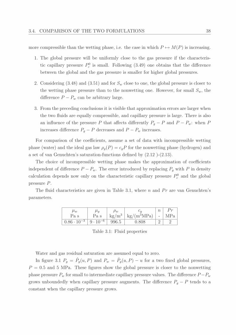
3.1 Fluid properties . . . . . . . . . . . . . . . . . . . . . . . . . . . . . . . . . 38
4.1 Test 1. Function parameters and rock properties . . . . . . . . . . . . . . . 58
4.2 Test 2. Function parameters and rock properties . . . . . . . . . . . . . . . 63
4.3 Test 3. Function parameters and rock properties . . . . . . . . . . . . . . . 66
v
List of Figures
2.1 Determination of the REV . . . . . . . . . . . . . . . . . . . . . . . . . . . 9
2.2 Determining the wetting fluid . . . . . . . . . . . . . . . . . . . . . . . . . 11
2.3 Capillary pressure for the van Genuchten and the Brooks and Corey models 14
2.4 Relative permeability functions in the van Genuchten and Brooks and Corey
models for Swr = Sgr = 0.05. . . . . . . . . . . . . . . . . . . . . . . . . . . 16
2.5 Capillary pressure with the entry pressure . . . . . . . . . . . . . . . . . . 23
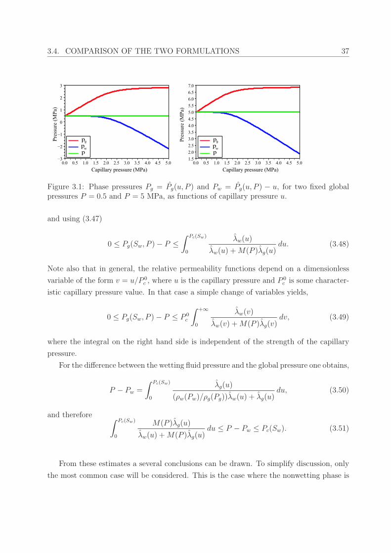
3.1 Phase pressures Pg = Pg(u, P ) and Pw = Pg(u, P ) − u, for two fixed global
pressures P = 0.5 and P = 5 MPa, as functions of capillary pressure u. . . 37
3.2 Comparison of the coefficients in the new and the simplified global pressure
models at the global pressure of 0.1 MPa. The coefficients are presented as
functions of the wetting phase saturation with fixed global pressure. . . . . 39
3.3 Comparison of the coefficients in the new and the simplified models at the
global pressure of 5 MPa. The coefficients are presented as functions of the
wetting phase saturation with fixed global pressure. . . . . . . . . . . . . . 40
4.1 Spatial mesh in one-dimensional case . . . . . . . . . . . . . . . . . . . . . 45
4.2 Test 1. Water saturation at different times . . . . . . . . . . . . . . . . . . 58
4.3 Test 1. Capillary pressure at different times . . . . . . . . . . . . . . . . . 58
4.4 Test 1. Global pressure at different times . . . . . . . . . . . . . . . . . . . 59
4.5 Test 1. Gas pressure at different times . . . . . . . . . . . . . . . . . . . . 59
4.6 Test 1. Water pressure at different times . . . . . . . . . . . . . . . . . . . 60
4.7 Test 1. Phase pressures and saturation on the left end . . . . . . . . . . . . 60
4.8 Test 2. Capillary pressures in the different domains . . . . . . . . . . . . . 62
4.9 Test 2. Water saturation at different times . . . . . . . . . . . . . . . . . . 63
4.10 Test 2. Global pressure at different times for the test case 2.1 (left) and test
case 2.2 (right) . . . . . . . . . . . . . . . . . . . . . . . . . . . . . . . . . 64
LIST OF FIGURES 1
4.11 Test 2. Gas pressure at different times for the test case 2.1 (left) and test
case 2.2 (right) . . . . . . . . . . . . . . . . . . . . . . . . . . . . . . . . . 64
4.12 Test 2. Water pressure at different times for the test case 2.1 (left) and test
case 2.2 (right) . . . . . . . . . . . . . . . . . . . . . . . . . . . . . . . . . 65
4.13 Test 2. Capillary pressure at different times for the test case 2.1 (left) and
test case 2.2 (right) . . . . . . . . . . . . . . . . . . . . . . . . . . . . . . . 65
4.14 Test 3. Water saturation at different times . . . . . . . . . . . . . . . . . . 67
4.15 Test 3. Global pressure at different times . . . . . . . . . . . . . . . . . . . 67
4.16 Test 3. Gas pressure at different times . . . . . . . . . . . . . . . . . . . . 67
4.17 Test 3. Water pressure at different times . . . . . . . . . . . . . . . . . . . 68
4.18 Test 3. Capillary pressure at different times . . . . . . . . . . . . . . . . . 68
5.1 Range of the mapping G2. . . . . . . . . . . . . . . . . . . . . . . . . . . . 80
A.1 UML diagram for the coefficients . . . . . . . . . . . . . . . . . . . . . . . 118
1
Chapter 1
Introduction
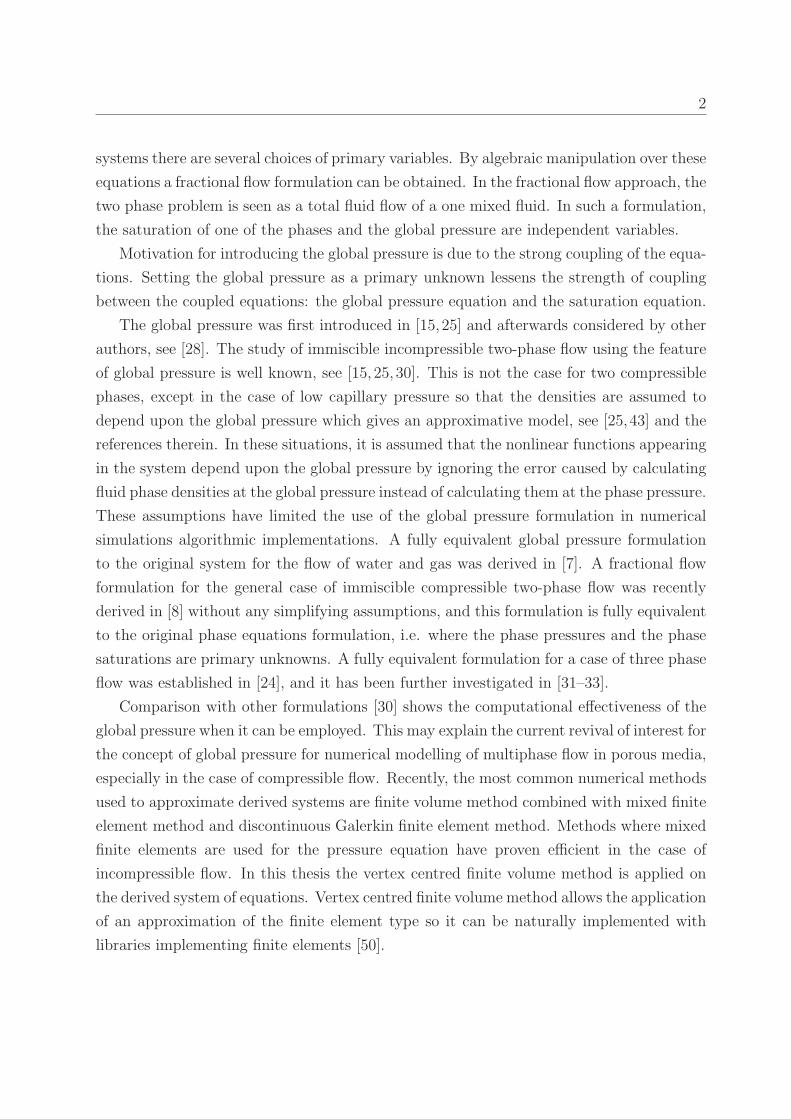
This work is closely related to the area of modelling of multiphase flow in porous me-
dia which is significant for many petroleum and environmental engineering problems. In
present-day industry, chlorinated hydrocarbons, petroleum products and similar materials
are essential and very frequent. Uncontrolled spreading of such materials may have strong
environmental influence. Furthermore, the storage of nuclear waste and recent advances
towards underground storage of CO2 additionally raise safety and environment concerns.
A certain risk of accidental spillage of harmful materials always exists. Such spills may
result in release of these materials into the environment, which may cause pollution of
the groundwaters. With regards to geological repositories of nuclear waste, problems are
related to the flow of water and gas. In such cases the gas is most commonly hydrogen
and the most important source of the gas is the corrosion of metallic components (waste
containers) and water radiolysis by radiation issued from nuclear waste. It is important
to model and predict underground gas migration, in order to avoid overpressure and pre-
vent mechanical damages. Mathematical models and numerical simulations of multiphase
flows help in the development of cost-efficient, safe and suitable methods for the storage
of hazardous materials. Numerical simulations of such models can give an answer about
the pressure, saturation and velocity of the fluids involved in the flow, as functions of the
space and time.
This thesis is devoted to the study of immiscible, compressible two-phase flow in porous
media, taking into account gravity, capillary effects, and heterogeneity. A general case of
two compressible fluids will be considered. The usual set of equations describing this type
of flow is given by the mass balance law and Darcy-Muscat law for each phase, which
leads to the system of strongly coupled nonlinear partial differential equations. In such
2
systems there are several choices of primary variables. By algebraic manipulation over these
equations a fractional flow formulation can be obtained. In the fractional flow approach, the
two phase problem is seen as a total fluid flow of a one mixed fluid. In such a formulation,
the saturation of one of the phases and the global pressure are independent variables.
Motivation for introducing the global pressure is due to the strong coupling of the equa-
tions. Setting the global pressure as a primary unknown lessens the strength of coupling
between the coupled equations: the global pressure equation and the saturation equation.
The global pressure was first introduced in [15,25] and afterwards considered by other
authors, see [28]. The study of immiscible incompressible two-phase flow using the feature
of global pressure is well known, see [15, 25, 30]. This is not the case for two compressible
phases, except in the case of low capillary pressure so that the densities are assumed to
depend upon the global pressure which gives an approximative model, see [25,43] and the
references therein. In these situations, it is assumed that the nonlinear functions appearing
in the system depend upon the global pressure by ignoring the error caused by calculating
fluid phase densities at the global pressure instead of calculating them at the phase pressure.
These assumptions have limited the use of the global pressure formulation in numerical
simulations algorithmic implementations. A fully equivalent global pressure formulation
to the original system for the flow of water and gas was derived in [7]. A fractional flow
formulation for the general case of immiscible compressible two-phase flow was recently
derived in [8] without any simplifying assumptions, and this formulation is fully equivalent
to the original phase equations formulation, i.e. where the phase pressures and the phase
saturations are primary unknowns. A fully equivalent formulation for a case of three phase
flow was established in [24], and it has been further investigated in [31–33].
Comparison with other formulations [30] shows the computational effectiveness of the
global pressure when it can be employed. This may explain the current revival of interest for
the concept of global pressure for numerical modelling of multiphase flow in porous media,
especially in the case of compressible flow. Recently, the most common numerical methods
used to approximate derived systems are finite volume method combined with mixed finite
element method and discontinuous Galerkin finite element method. Methods where mixed
finite elements are used for the pressure equation have proven efficient in the case of
incompressible flow. In this thesis the vertex centred finite volume method is applied on
the derived system of equations. Vertex centred finite volume method allows the application
of an approximation of the finite element type so it can be naturally implemented with
libraries implementing finite elements [50].
3
Discontinuous porous media is a special problem for numerical methods, since at the
discontinuities the fluxes and (in general) phase pressures are continuous through the dis-
continuity of the medium, which would generally produce discontinuities in the main un-
knowns of the derived system. All these values need to be calculated locally, from the
globally assigned values. The discontinuous media has been a problem of study of many
authors, see [17,46,54–56,59].
Mathematical analysis of the two-phase flow in porous media has been a problem
of interest for many years and many methods have been developed. One may refer
to [6, 15, 16, 20, 25, 27, 36, 38, 40, 49, 66, 67] for more information on the analysis, espe-
cially on the existence of solutions of immiscible incompressible two-phase flow in porous
media. The case of miscible compressible flow in porous media is treated in [10–12,34,39].
However, the situation is quite different for immiscible compressible two-phase flow in
porous media, where only recently a few results were obtained. In the case of immiscible
two-phase flows with one (or more) compressible fluids without any exchange between the
phases, some approximate models were studied in [41–43]. In [41] certain terms related
to the compressibility are neglected, and in [42, 43] the mass densities are assumed not
to depend on the physical pressure, but on the Chavent’s global pressure. In [44, 48], a
more general immiscible compressible two-phase flow model in homogeneous porous media
is considered with the assumption of the bounded capillary pressure function, which is too
restrictive for some realistic problems. In the case of immiscible two-phase flows with one
(or more) compressible fluids with the exchange between the phases, i.e. a multicomponent
model, the existence of weak solutions for these equations under some assumptions on the
compressibility of the fluids has been recently established in [51,62,63].
This thesis is organized as follows: in chapter 2 basic terms and equations on the de-
scription of the two-phase flow model in porous media are presented [17–19, 25, 30, 46].
At the end of the chapter several formulations of the model are presented with different
primary variables chosen. Also, since most of the simulations in chapter 4 involve het-
erogeneous porous medium, general treatment of the heterogeneity in the porous media is
discussed.
A new model using global pressure as a primary variable, fully equivalent to original
equations, derived in chapter 2, is described in chapter 3. The new model was introduced
in [7] for water-gas flow. In this chapter, the model is presented for the flow of two com-
pressible fluids, and is mainly represented in the article [8]. By setting the global pressure
as primary variable in the new fractional flow formulation, a computation of phase pres-
4
sures corresponding to a given global pressure requires a solution of a differential equation
(see (3.14)). The evaluation of the coefficients depending on phase pressures requires more
calculation in the fully equivalent fractional flow model (3.23)–(3.25) as compared to the
original model (2.20), (2.21). Numerically, this calculation can be performed by using
standard numerical libraries present in the literature. For this reason, a simplified frac-
tional flow formulation, which is not fully equivalent to the corresponding phase equations,
is presented. The simplified fractional flow formulation is compared to fully equivalent
fractional flow formulation by comparing the coefficients. The goal of the comparison is to
recognize situations in which approximate fractional flow formulation can be safely used
and to show differences in approximate and fully equivalent formulations in the cases where
these are significant.
In chapter 4 the finite volume method in one dimensional case for the new model is
presented. Special attention is paid to the treatment of the heterogeneities. In numerical
simulations, the fluids observed are water, considered as incompressible, and compressible
gas, such as hydrogen, concerning the gas migration through engineered and geological
barriers for the deep repository of radioactive waste. In the development and usage of
numerical models for immiscible compressible flow in porous media it is important to
verify the numerical model by means of adequate benchmark problems.
Recently, the French research group MoMaS (http://www.gdrmomas.org/) proposed
benchmark tests (http://www.gdrmomas.org/ex qualifications.html) designed to improve
the simulation of the water–hydrogen flow related to corrosion of nuclear waste containers
in an underground storage.
The verification of the new global pressure model is shown on several test cases [52]
in the heterogeneous porous media. In the first test case, the initial conditions for phase
pressures are taken to be continuous and constant in the whole domain, so that the capillary
pressure is continuous and nonzero at the initial moment. The new and the simplified model
are applied to this test case, and the results are compared afterwards. In the second test
case, the initial capillary pressure is taken to be discontinuous, and the intensity of the
capillary pressure is taken to be very high compared to the initial gas pressure, which can
lead to numerical difficulties. The third test case is chosen to represent the effect of the
entry pressure, when the porous medium is initially fully saturated by the water.
In chapter 5 existence results of weak solutions for this new formulation for the two-
phase compressible flows are obtained. This section contains results from [9]. The equations
are rewritten by expressing the phase fluxes in terms of nonwetting saturation and global

5
pressure. Under certain realistic assumptions on the data also presented in this chapter,
an existence result, with the help of appropriate regularizations and the time discretization
is obtained. The system is firstly regularized with a parameter η > 0 in order to make
capillary pressure bounded, and a small constant is added to diffusivity term to obtain the
ellipticity of the discretized system. The existence of the weak solution for a regularized
system is shown, by introducing time discretization, so a small parameter h > 0 relating
to the time discretization is introduced. Afterwards, the existence of the solution for a
discretized problem is shown by applying Schauder’s fixed point theorem. A set of suitable
test functions is employed to get a priori estimates independent on h and the regularization
parameter η, in order to pass to the limit in nonlinear terms when h tends to zero. This
gives the existence result for a regularized system. To pass to the limit as η tends to zero a
generalization of compactness lemma from [25,43,48] and a compactness lemma from [60]
is used. This approach permits considering heterogeneous media.
Appendix A contains further explanation on the implementation of the coefficients
of the fully equivalent global pressure formulation of compressible, immiscible two-phase
flow. The numerical code for their calculation is developed and implemented in C++
programming language.

6
Chapter 2
Two-phase Flow in Porous Media
In this chapter the basic terms and equations for immiscible compressible two-phase fluid
flow in porous media are explained. The chapter is organized as follows: in the first section
the basic terms and laws regarding the porous media are presented. The second section is
devoted to two-phase immiscible compressible flow, and explanation of the terms needed
to describe this flow. The third section starts with the presentation of the governing
equations describing two-phase immiscible flow in porous media, written on macroscopic
level, and afterwards some basic formulations are presented. At the end of the chapter, the
treatment of the heterogeneous porous media is considered. Most of this chapter follows
the references [19], [17], [25], [46].
2.1 Porous Media
2.1.1 Basic Definitions
Every material composed of a solid part called solid matrix and a connected pore space
(void space) can be identified as a porous medium. The pore space can be filled with
one or more fluids. In order to derive valid mathematical model of fluid flow through a
porous medium, the medium must satisfy some additional properties [35], [17]:
• Pore space is interconnected.
• The smallest dimension of the pore space must be large enough to contain fluid par-
ticles. This property allows the application of the continuum approach at the pore
space scale.
2.1. POROUS MEDIA 7
• Dimensions of the pore space must be small enough so that the fluid flow is controlled
by adhesive forces of fluid-solid interfaces and cohesive forces of fluid-fluid interfaces.
This property eliminates the case of network pipes.
Some of the examples of the porous media are: sand, soil, clay, sponge, etc.
If the pore space is filled by a single, or by several, completely miscible fluids, one speaks
about single-phase fluid flow in porous media. The term phase, as employed in [46] is used
to differentiate one or more fluids separated by a sharp interface. Two fluids are said to
be immiscible if a strictly defined interface between them exists. In such a system, each
fluid represents a different phase. The solid matrix is considered to be the solid phase.
Different phase properties are assigned to each phase, one fluid phase may differ from the
others by its density, dynamic viscosity and compressibility. Phases can also be composed
of different components. However, multicomponent flows are not considered in the scope
of this work. Further details may be found in [17,25,46].
2.1.2 Fluid Properties
Mass density of the fluid will be denoted by ρ. Generally, it is assumed to be a function
of the fluid pressure P , and temperature T . In this work, only the isothermal flow is con-
sidered, which means that it is assumed that the density depends only upon the pressure,
and temperature T is involved only as a parameter. The density is constant if the fluid is
incompressible. In the case of the ideal gas the density is given by the equation of the
state:
ρ(P ) =PM
RT,
where R is the universal gas constant (R = 8.31J/Kmol), T is the temperature, and M is
the fluid molar mass.
Compressibility of the fluid is defined as
ν =1
ρ(P )
dρ(P )
dP.
It is usually assumed to be a constant so, generally, the density can be given as
ρ(P ) = ρ0eν(P−P0),
2.1. POROUS MEDIA 8
where P0 is the reference pressure and ρ0 = ρ(P0).
In the case of liquids, ν is usually assumed to be very low. For example, the compress-
ibility of water is 5.1 × 10⁻¹⁰Pa−1. Fluids with low compressibility can be modeled as
incompressible, or the density is modeled as
ρ(P ) = ρ0 + ν(P − P0) (2.1)
Such fluids are called slightly compressible fluids.
Another property of the fluid is dynamic viscosity [Pas, cP ] which, in this work, will
be called simply viscosity. In this work it is assumed constant, though it can also depend
on pressure and temperature.
2.1.3 Macroscopic Scale
In the mathematical modelling of flow through porous media, different scales can be used.
Besides molecular scale (≈ 10−9m) one can use microscopic and macroscopic scale.
At the microscopic scale the system of Navier-Stokes equations is used, with some
assigned boundary conditions. The task of solving the Navier-Stokes equations in the pore
space is not practical due to the unknown pore space geometry. Moreover, the fluid flow
variations at the pore space scale, are not of interest. Therefore, one needs to set up
mathematical model at a larger scale.
Because of these reasons, the macroscopic scale is usually used, and in the flow de-
scription a continuum approach is applied. At the macroscopic scale, the porous medium
is assumed to be a continuum in which one does not distinguish the solid phase from the
fluid phases present in the pore space. On macroscopic level, macroscopic quantities repre-
sent average values of the quantities given on the microscopic level. Therefore, quantities
appearing in the macroscopic model, i.e. pressure and velocity, actually represent average
values over sufficiently large volumes.
Porous medium is called homogeneous if its properties do not vary in space or time.
Otherwise, the medium is called heterogeneous.
2.1. POROUS MEDIA 9
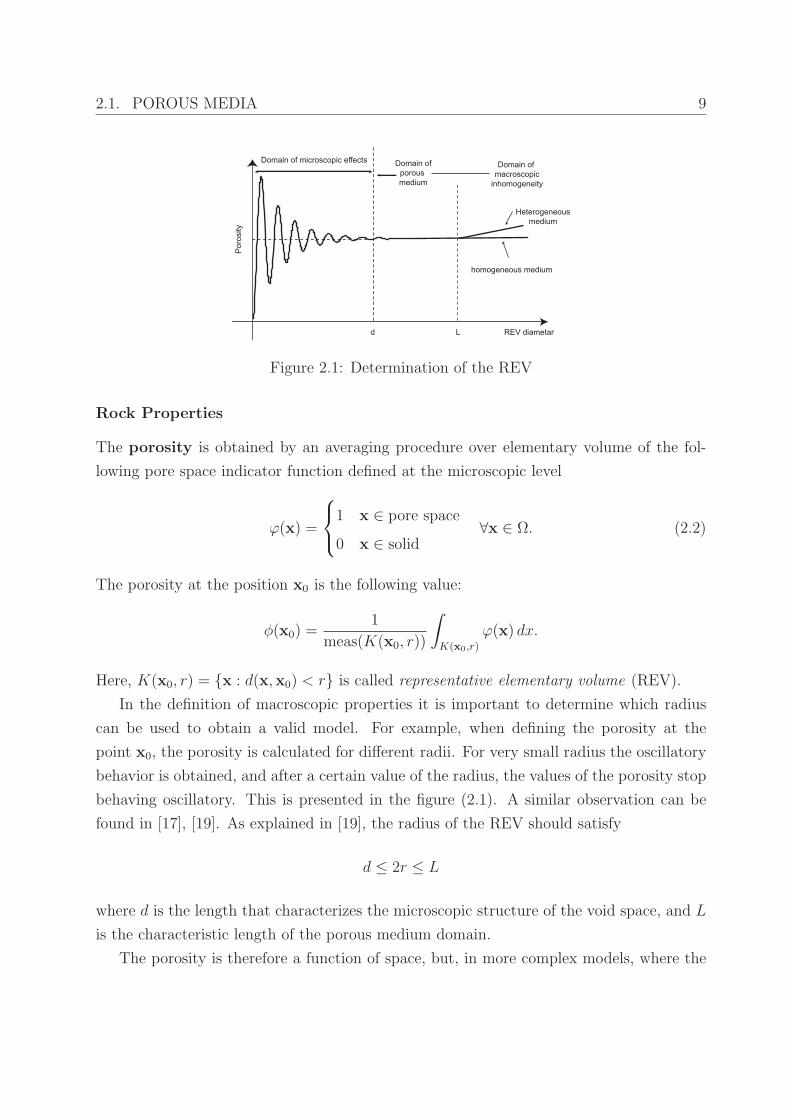
Figure 2.1: Determination of the REV
Rock Properties
The porosity is obtained by an averaging procedure over elementary volume of the fol-
lowing pore space indicator function defined at the microscopic level
ϕ(x) =
1 x ∈ pore space
0 x ∈ solid∀x ∈ Ω. (2.2)
The porosity at the position x0 is the following value:
φ(x0) =1
meas(K(x0, r))
∫
K(x0,r)
ϕ(x) dx.
Here, K(x0, r) = x : d(x,x0) < r is called representative elementary volume (REV).
In the definition of macroscopic properties it is important to determine which radius
can be used to obtain a valid model. For example, when defining the porosity at the
point x0, the porosity is calculated for different radii. For very small radius the oscillatory
behavior is obtained, and after a certain value of the radius, the values of the porosity stop
behaving oscillatory. This is presented in the figure (2.1). A similar observation can be
found in [17], [19]. As explained in [19], the radius of the REV should satisfy
d ≤ 2r ≤ L
where d is the length that characterizes the microscopic structure of the void space, and L
is the characteristic length of the porous medium domain.
The porosity is therefore a function of space, but, in more complex models, where the
2.1. POROUS MEDIA 10
rock is deformable, it is assumed to be a function of the pressure.
Another macroscopic property of the porous medium is the absolute permeability K
[m2,Darcy], usually a symmetric tensor describing the ability of the porous media to trans-
mit fluids. In the heterogeneous media it is space dependent and the media is isotropic
if K = kI.
The absolute permeability appears in Darcy’s law, which will be described in the next
subsection. In the two-phase flow system, besides the absolute permeability, the relative
permeabilities must be introduced, since the flow of each phase depends upon the presence
of other phases.
2.1.4 Derived Macroscopic Equations
At the macroscopic level, the macroscopic balance law for the one-phase system in a
porous medium Ω ⊆ Rn can be rewritten as [17], [25]:
∂(Φρ(P ))
∂t+ div(ρ(P )q) = F (2.3)
where q [m/day] is a macroscopic apparent velocity, and F is a source (sink) term.
The macroscopic apparent velocity or Darcy velocity q [m/year] relates to the pressure
of the fluid with the equation called Darcy’s law.
q = − 1
µK(∇P − ρg) (2.4)
where g is the gravitational, downward-pointing, constant vector and, as already men-
tioned, ρ is the fluid density, and P is the fluid pressure. Darcy’s law is actually the
momentum conservation of the Navier-Stokes equation on the macroscopic level [17].
Therefore, the equation which describes monophasic flow in the porous domain Ω ⊆ Rn,
with P as unknown (and q as unknown which is calculated by Darcy’s law) is:
∂(Φρ(P ))
∂t− div(
ρ(P )
µK (∇P − ρ(P )g)) = F , in Ω. (2.5)
2.2. TWO-PHASE FLOW IN POROUS MEDIA 11
To this equation the following initial and boundary conditions are usually assigned:
P (x, 0) = P0(x), P (x, t) = Pd(x, t) on Γd ρq · n = qn on Γn,
where ∂Ω = Γd ∪ Γn.
In the case of incompressible fluid flow, the initial condition for the pressure is not
necessary, since in that case one deals with an elliptic equation. Equations (2.4)-(2.3) can
also be rewritten for the case of a two-phase flow. In that case, however, several additional
definitions are needed. These will be presented in the next section.
2.2 Two-phase Flow in Porous Media
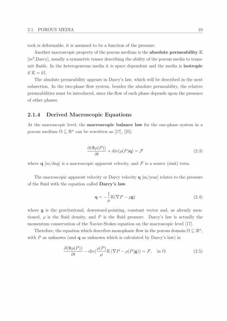
In the two-phase flow system, a wetting and a nonwetting phase are introduced. One
example of this kind of system is water-gas system, where the water is the wetting phase.
In the flow of oil and water, water is considered as a wetting phase, and in the flow of oil and
gas, oil is considered to be the wetting fluid. The wetting phase can be easily determined
by the following action: if one looks at a capillary tube, the convexity of meniscus is always
oriented towards wetting fluid, as presented in the figure (2.2). In this work the indices
Figure 2.2: Determining the wetting fluid
α = w, g, will denote the wetting and nonwetting phases respectively. To rewrite the
equations (2.3) and (2.4) in a two-phase flow case one needs to introduce aditional terms:
saturations, capillary pressure and relative permeabilities.
2.2.1 Saturation
Phase saturations Sα, α = w, g are macroscopic variables introduced in order to describe
the quantity of the volume of the phase at the point x0 of the porous medium. Its definition
is similar to the definition of the porosity. For a phase α = w, g the phase indicator function
is [17]:

2.2. TWO-PHASE FLOW IN POROUS MEDIA 12
ϕα(x, t) =
1 x ∈ phase α at time t
0 x /∈ phase α at time t
The saturation of the phase α is defined as
Sα(x0, t) =
∫
REVϕα(x,t) dx
∫
REVϕ(x) dx
. ∀x0 ∈ Ω
where ϕ(x) is the function defined by (2.2), and REV is assigned to the point x0
It clearly follows∑
α Sα(x, t) = 1, and 0 ≤ Sα ≤ 1, α = w, g.
2.2.2 Capillary Pressure
On the microscopic level two immiscible fluids are separated by clearly defined interface
which leads to a jump of pressure. This jump of pressure is called capillary pressure and
is equal to
Pc = Pg − Pw. (2.6)
It is described by
Pc = σ
(
1
r1+
1
r2
)
(2.7)
where σ is the interfacial tension, and r1 and r2 are the main curvature radii of the surface
between the fluids. For smaller meniscus radii the capillary pressure is higher and vice
versa, for larger radii the capillary pressure is lower. One can conclude from this, that,
in the case of drainage - injection of the nonwetting phase in the area fully saturated by
the wetting phase - the wetting phase flows to smaller pores. On the contrary, when the
imbibition -injection of the wetting phase in the area fully saturated by the nonwetting
phase - is performed the wetting phase starts to fill the largest pores first.
Capillary pressure is always positive since the pressure of the nonwetting phase is higher
than the pressure of the wetting phase.
Macroscopic capillary pressure is an average value of the microscopic capillary pressure.
On the macroscopic level, there is no interface between phases, and in every point of the
2.2. TWO-PHASE FLOW IN POROUS MEDIA 13
porous medium domain one observes wetting and nonwetting pressure Pw and Pg, and
these are the average values of the values of the fluid pressures defined on the microscopic
level. Thus the equation (2.6) is also valid at the macroscopic level.
The macroscopic capillary pressure is assumed to depend on the saturation since, for ex-
ample, when drainage is performed one can conclude from the previous discussion that the
decrease of wetting phase saturation would produce the increase of the capillary pressure.
The values of capillary pressure function can be obtained experimentally by performing
drainage, or by performing imbibition. Since the measurements require certain amount of
time, theoretical formulae are commonly used in practice.
When the saturation of the wetting phase in the porous medium is equal to a cer-
tain small value Swr, the increase of the gas pressure will not displace the wetting phase.
Value Swr is called the residual saturation of the wetting phase. The capillary pressure
is expected to have vertical asymptote at that point. Similarly, in the case of imbibition,
certain amount of nonwetting phase that cannot be displaced by a wetting phase exists,
so the saturation of the nonwetting phase cannot be lower than Snr, (the residual non-
wetting saturation). Therefore, the capillary pressure is naturally defined on the interval
]Swr, 1 − Snr] .
It is natural to introduce the effective saturation
Sew =Sw − Swr
1 − Swr − Sgr
Seg =Sg − Sgr
1 − Swr − Sgr
(2.8)
which means that
Sw = Swr ⇒ Sew = 0 and Sw = 1 − Sgr ⇒ Sew = 1
and clearly:
Sew + Seg = 1.
The capillary pressure is usually considered to be a function of the effective saturation.
Several analytical expressions of the capillary pressure exist. The two most important,
usually used in the description of water-gas flows are:
• Van Genuchten capillary pressure [64]
Pc(Sew) = Pr(S−
1m
ew − 1)1n Sew ∈ ]0, 1] , (2.9)
2.2. TWO-PHASE FLOW IN POROUS MEDIA 14
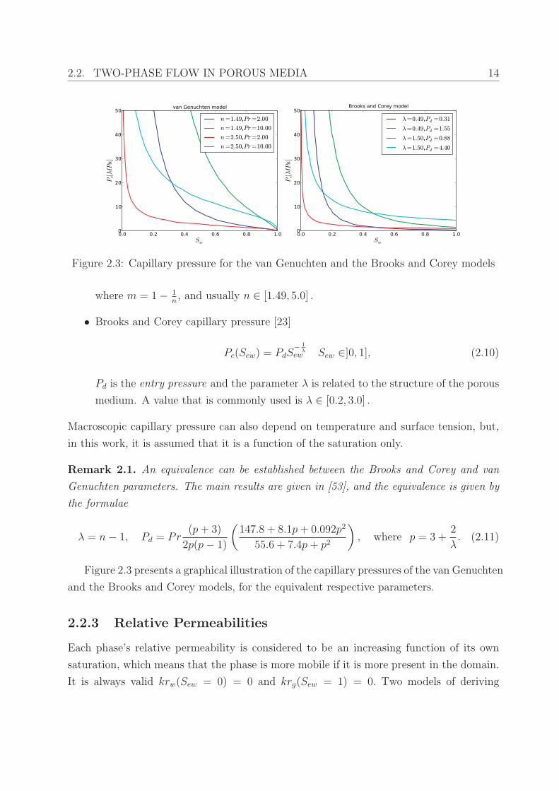
Figure 2.3: Capillary pressure for the van Genuchten and the Brooks and Corey models
where m = 1 − 1n, and usually n ∈ [1.49, 5.0] .
• Brooks and Corey capillary pressure [23]
Pc(Sew) = PdS−
1λ
ew Sew ∈]0, 1], (2.10)
Pd is the entry pressure and the parameter λ is related to the structure of the porous
medium. A value that is commonly used is λ ∈ [0.2, 3.0] .
Macroscopic capillary pressure can also depend on temperature and surface tension, but,
in this work, it is assumed that it is a function of the saturation only.
Remark 2.1. An equivalence can be established between the Brooks and Corey and van
Genuchten parameters. The main results are given in [53], and the equivalence is given by
the formulae
λ = n− 1, Pd = Pr(p+ 3)
2p(p− 1)
(
147.8 + 8.1p+ 0.092p2
55.6 + 7.4p+ p2
)
, where p = 3 +2
λ. (2.11)
Figure 2.3 presents a graphical illustration of the capillary pressures of the van Genuchten
and the Brooks and Corey models, for the equivalent respective parameters.
2.2.3 Relative Permeabilities
Each phase’s relative permeability is considered to be an increasing function of its own
saturation, which means that the phase is more mobile if it is more present in the domain.
It is always valid krw(Sew = 0) = 0 and krg(Sew = 1) = 0. Two models of deriving

2.2. TWO-PHASE FLOW IN POROUS MEDIA 15
the relative permeability functions form the given capillary pressure function are described
here, (Mualem’s and Burdine’s). More detailed presentations of these models can be found
in [26], [46].
• In the Mualem model, relative permeability functions are defined by the following
formulae
krw(Sew) = S12ew
(∫ Sew
0ds
Pc(s)∫ 1
0ds
Pc(s)
)2
(2.12)
krg(Sew) = (1 − Sew)12
(∫ 1
Sew
dsPc(s)
∫ 1
0ds
Pc(s)
)2
. (2.13)
• In the Burdine model, relative permeability functions are defined by the following
formulae
krw(Sew) = S2ew
(∫ Sew
0ds
P 2c (s)
∫ 1
0ds
P 2c (s)
)
(2.14)
krg(Sew) = (1 − Sew)2
(∫ 1
Sew
dsP 2
c (s)∫ 1
0ds
P 2c (s)
)
. (2.15)
Calculation gives the following van Genuchten Mualem relative permeability functions:
krw(Sew) =S12ew
(
1 − (1 − S1mew)m
)2
(2.16)
krg(Sew) =(1 − Sew)12 (1 − S
1mew)2m. (2.17)
Also, the following Brooks and Corey Burdine functions are obtained:
krw(Sew) = S3+ 2
λew (2.18)
krg(Sew) = (1 − Sew)2(
1 − S2+λ
λew
)
. (2.19)
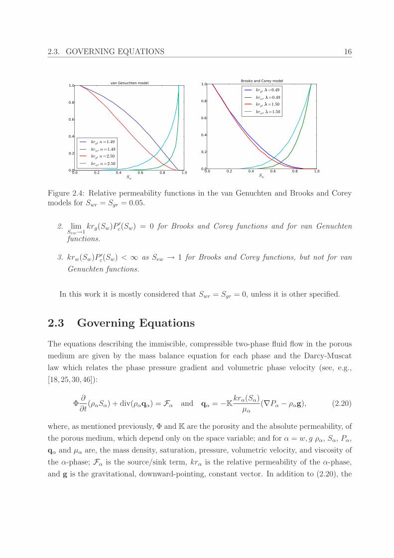
These functions are presented in the figure 2.4 for the Swr = Sgr = 0.05.
Remark 2.2. For the formulae (2.16)-(2.19) one obtains:
1. limSew→0
krw(Sw)P ′
c(Sw) = 0 for Brooks and Corey functions and for van Genuchten
functions.
2.3. GOVERNING EQUATIONS 16
0.0 0.2 0.4 0.6 0.8 1.0Sw
0.0
0.2
0.4
0.6
0.8
1.0Brooks and Corey model
krg, =0.49
krw, =0.49
krg, =1.50
krw, =1.50
Figure 2.4: Relative permeability functions in the van Genuchten and Brooks and Coreymodels for Swr = Sgr = 0.05.
2. limSew→1
krg(Sw)P ′
c(Sw) = 0 for Brooks and Corey functions and for van Genuchten
functions.
3. krw(Sw)P ′
c(Sw) < ∞ as Sew → 1 for Brooks and Corey functions, but not for van
Genuchten functions.
In this work it is mostly considered that Swr = Sgr = 0, unless it is other specified.
2.3 Governing Equations
The equations describing the immiscible, compressible two-phase fluid flow in the porous
medium are given by the mass balance equation for each phase and the Darcy-Muscat
law which relates the phase pressure gradient and volumetric phase velocity (see, e.g.,
[18, 25,30,46]):
Φ∂
∂t(ραSα) + div(ραqα) = Fα and qα = −K
krα(Sα)
µα
(∇Pα − ραg), (2.20)
where, as mentioned previously, Φ and K are the porosity and the absolute permeability, of
the porous medium, which depend only on the space variable; and for α = w, g ρα, Sα, Pα,
qα and µα are, the mass density, saturation, pressure, volumetric velocity, and viscosity of
the α-phase; Fα is the source/sink term, krα is the relative permeability of the α-phase,
and g is the gravitational, downward-pointing, constant vector. In addition to (2.20), the
2.3. GOVERNING EQUATIONS 17
following equations apply
Sw + Sg = 1, and Pc(Sw) = Pg − Pw. (2.21)
The primary variables are Sα, Pα, and qα. Here the porosity Φ and the absolute permeabil-
ity K are functions of space and the viscosities µw, µg are constant. Finally, the capillary
pressure and relative permeabilities are considered to be functions of the saturation only.
To simplify the notation their spatial dependence is omitted. The governing equations
(2.20)–(2.21) are strongly coupled, nonlinear partial differential equations. These equa-
tions can be transformed in other forms (see [29], [30]) by algebraic manipulation over
these equations and choice of primary unknowns.
2.3.1 Pressure-Pressure Formulation
In the system (2.20)-(2.21) one may select phase pressures as the main unknowns. Given
that the capillary pressure is an invertible function, the phase saturations are
Sα = Sα(Pc) = Sα(Pg − Pw).
Thus the governing equations can be reformulated in the following way
Φ∂
∂t(ρg(Pg)Sg(Pg − Pw)) + div(ρg(Pg)qg) = Fg (2.22)
Φ∂
∂t(ρw(Pw)Sw(Pg − Pw)) + div(ρw(Pw)qw) = Fw (2.23)
qg = −Kkrg(Sg(Pg − Pw))
µg
(∇Pg − ρg(Pg)g) (2.24)
qw = −Kkrw(Sw(Pg − Pw))
µw
(∇Pw − ρw(Pw)g). (2.25)
The derived system is strongly coupled through the expression for the saturation. This
formulation is not commonly used [46], since it is inefficient for very small capillary pressure
gradients, which often occur in heterogeneous porous media.
2.3. GOVERNING EQUATIONS 18
2.3.2 Pressure-Saturation Formulation
This approach will be explained on a system where the wetting phase saturation and the
nonwetting pressure are chosen as main unknowns. From (2.21) one easily obtains
Sg = 1 − Sw Pw = Pg − Pc(Sw).
Putting this into (2.20) the following system of equations in the porous domain Ω ⊆ Rnis
obtained:
Φ∂
∂t(ρg(Pg)(1 − Sw)) + div(ρg(Pg)qg) = Fg (2.26)
Φ∂
∂t(ρw(Pw)Sw) + div(ρw(Pw)qw) = Fw (2.27)
qg = −Kkrg(Sw)
µg
(∇Pg − ρg(Pg)g) (2.28)
qw = −Kkrw(Sw)
µw
(∇Pg −∇Pc(Sw) − ρw(Pw)g) (2.29)
The derived system is strongly coupled and it can be assumed as a parabolic system. By
reformulation, one can see that this is not true [17]. The boundary and initial conditions
can be chosen as [17]:
Sw(x, 0) = S0w(x) Pg(x, 0) = P 0
g (x) x ∈ Ω (2.30)
Sw(x, t) = Sdw(x, t) on ΓSw
d Pg(x, t) = P dg (x, t) on Γ
Pg
d (2.31)
ρw(Pw)qw · n = Qw on ΓSwn ρg(Pg)qg · n = Qg on ΓPg
n (2.32)
Note that in the above: ∂Ω = ΓPg
d ∪ ΓPgn = ΓSw
d ∪ ΓSwn .
In order to reveal the type of the system (2.26)-(2.29), it is worthwhile to examine
an another formulation which also includes one pressure, and one saturation as the main
unknowns. Therefore, the phase mobility functions are introduced:
λα(Sw) =krα(Sw)
µα
, α = w, g (2.33)
and the total mobility is
λ(Sw, Pg) = ρw(Pw)λw(Sw) + ρg(Pg)λg(Sw). (2.34)
2.3. GOVERNING EQUATIONS 19
Then the fractional flow functions
fα(Sw, Pg) =ρα(Pα)λα(Sw)
λ(Sw, Pg), α = w, g, (2.35)
and also the following nonlinear functions:
ρ(Sw, Pg) =(λw(Sw)ρw(Pw)2 + λg(Sw)ρg(Pg)
2)
λ(Sw, Pg), (2.36)
α(Sw, Pg) =ρw(Pw)ρg(Pg)λw(Sw)λg(Sw)
λ(Sw, Pg), (2.37)
bg(Sw, Pg) = (ρw(Pw) − ρg(Pg))α(Sw, Pg), a(Sw, Pg) = −α(Sw, Pg)P′
c(Sw). (2.38)
are introduced. In the above formulae the nonwetting pressure Pg and the wetting phase
saturation Sw are chosen as independent variables.
Rewriting the equations (2.20)–(2.21) by summation of the two equations and intro-
duction of total flux, Qt = ρw(Pw)qw + ρg(Pg)qg, one obtain the following:
Φ∂
∂t(Swρw(Pw) + (1 − Sw)ρg(Pg))
− div (λ(Sw, Pg)K [∇Pg − fw(Sw, Pg)∇Pc(Sw) − ρ(Sw, Pg)g]) = Fw + Fg,(2.39)
Qt = −λ(Sw, Pg)K (∇Pg − fw(Sw, Pg)∇Pc(Sw) − ρ(Sw, Pg)g) , (2.40)
Φ∂
∂t(ρw(Pw)Sw)+div(fw(Sw, Pg)Qt + bg(Sw, Pg)Kg)−div(a(Sw, Pg)K∇Sw) = Fw. (2.41)
The governing equation for the saturation (2.41) is a nonlinear convection-diffusion PDE
and the equation for pressure (2.39) is a nonlinear PDE strongly coupled to the saturation
equation through the gradient of capillary pressure and the time derivative term. The
boundary and initial conditions for this system can be again defined with (2.30)-(2.32).
Remark 2.3. Phase fluxes can be expressed through the total flux as:
ρw(pw)qw = fw(Sw, Pg)Qt − a(Sw, Pg)K∇Sw + bg(Sw, Pg)Kg, (2.42)
ρg(Pg)qg = fg(Sw, Pg)Qt + a(Sw, Pg)K∇Sw − bg(Sw, Pg)Kg. (2.43)
Remark 2.4. Starting with the (Sg, Pw) formulation the coefficients (2.33)-(2.38) may
be rewritten as a functions of the variables (Sg, Pw) by changing the variable as follows:
Sg = 1−Sw and Pw = Pg −Pc(Sg). This way one obtain the following system of equations:
2.3. GOVERNING EQUATIONS 20
Φ∂
∂t((1 − Sg)ρw(Pw) + Sgρg(Pg))
− div (λ(Sg, Pw)K [∇Pw + fg(Sw, Pw)∇Pc(Sg) − ρ(Sg, Pw)g]) = Fw + Fg,(2.44)
Qt = −λ(Sg, Pw)K (∇Pw + fg(Sg, Pw)∇Pc(Sg) − ρ(Sg, Pw)g) , (2.45)
Φ∂
∂t(ρg(Pg)Sg) + div(fg(Sw, Pw)Qt − bg(Sg, Pw)Kg) − div(a(Sg, Pw)K∇Sg) = Fg. (2.46)
Incompressible Case
In the case where the two fluids in the porous medium are incompressible, the mass balance
law for each phase can be divided by the phase density. By introducing the total velocity
qt = qw + qg
and the coefficients
λinc(Sw) = λw(Sw) + λg(Sw)
f incw (Sw) = λw(Sw)/λinc(Sw) fg(Sw) = λg(Sw)/λinc(Sw)
ρinc(Sw) = (λw(Sw)ρw + λg(Sw)ρg)/λinc(Sw)
αinc(Sw) = λw(Sw)λg(Sw)/λinc(Sw)
bg(Sw) = (ρw − ρg)αinc(Sw)
a(Sw) = −αinc(Sw)P ′
c(Sw).
one obtains the following equations:
div(qt) = Fw/ρw + Fg/ρg (2.47)
Φ∂Sw
∂t+ div(f inc
w (Sw)qt + Kgbincg (Sw)) − div(ainc(Sw)K∇Sw) = Fw/ρw. (2.48)
where
qt = −λinc(Sw)K[
∇Pg − f incw (Sw)P ′
c(Sw)∇Sw − ρinc(Sw)g]
(2.49)
2.4. DISCONTINUOUS POROUS MEDIA. INTERFACE CONDITIONS 21
and the following expressions for the velocities:
qw = f incw (Sw)qt − Kainc(Sw)∇Sw + Kgbinc
g (Sw)
qg = f incg (Sw)qt + Kainc(Sw)∇Sw − Kgbinc
g (Sw).
One can see that in the incompressible case the coupling between the two equations is
less strong since the time derivative term does not appear in equation (2.47). It is shown
[15,25](see also section 3.1 ) that by introducing a new variable called global pressure this
coupling can be weaken even more, giving the system well defined mathematical structure.
2.4 Discontinuous Porous Media. Interface Condi-
tions
Porous media are usually heterogeneous, which introduces additional difficulties in mathe-
matical modelling, since the heterogeneity must be treated properly, and some additional
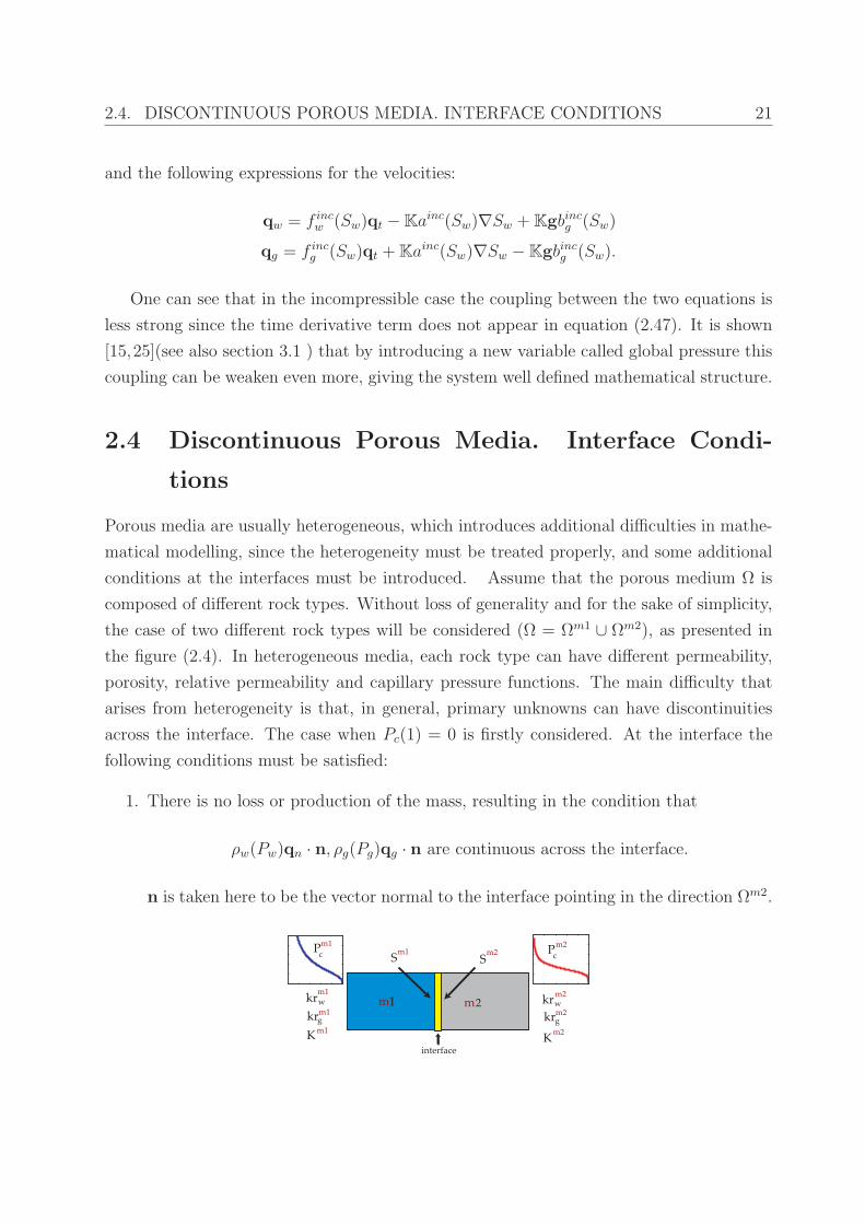
conditions at the interfaces must be introduced. Assume that the porous medium Ω is
composed of different rock types. Without loss of generality and for the sake of simplicity,
the case of two different rock types will be considered (Ω = Ωm1 ∪ Ωm2), as presented in
the figure (2.4). In heterogeneous media, each rock type can have different permeability,
porosity, relative permeability and capillary pressure functions. The main difficulty that
arises from heterogeneity is that, in general, primary unknowns can have discontinuities
across the interface. The case when Pc(1) = 0 is firstly considered. At the interface the
following conditions must be satisfied:
1. There is no loss or production of the mass, resulting in the condition that
ρw(Pw)qn · n, ρg(Pg)qg · n are continuous across the interface.
n is taken here to be the vector normal to the interface pointing in the direction Ωm2.
2.4. DISCONTINUOUS POROUS MEDIA. INTERFACE CONDITIONS 22
2. If the two-phase system is present at each side of the interface, and both phases
are mobile (which means λw(Sw), λg(Sg) > 0), it is assumed that the intensive state
variables are continuous at the interface, which means that the phase and capillary
pressures satisfy:
Pm1c (xinterface, t) = Pm2
c (xinterface, t)
Pm1g (xinterface, t) = Pm2
g (xinterface, t)
Pm1w (xinterface, t) = Pm2
w (xinterface, t)
The second condition is derived from the boundedness of the phase fluxes, in the case when
both phases are mobile at the interface.
The consequence of the continuity of the capillary pressure is that the saturation vari-
able is generally discontinuous at the interface, and has two limiting values Sm1w and Sm2
w
in the interface point.
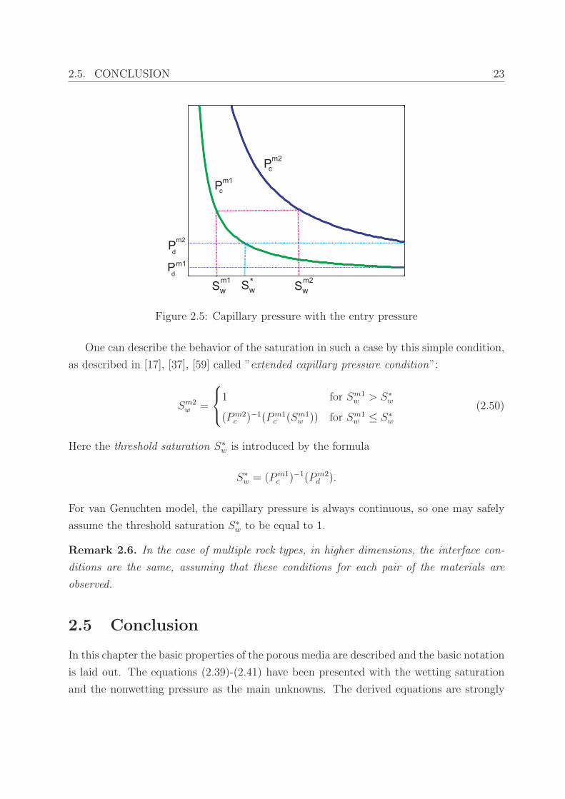
However, a common situation is having the entry pressure involved in the model de-
scribing capillary pressure (like in Brooks and Corey capillary pressure) which means
Pc(1) = Pd.
In such a case capillary pressure does not need to be continuous. One can observe situations
like the one presented in the figure 2.5, where the entry pressures for different rock types
are not the same. In these situations one phase pressure is also discontinuous, since the
phase and capillary pressures are connected by the equation (2.21).
Remark 2.5. As described in [37] when the porous media is initially saturated by the
wetting phase, and the nonwetting phase is injected, the meaning of the ”entry pressure”,
can be described as follows: the nonwetting phase will cross the interface only when the
capillary pressure Pm1c is greater then the entry pressure Pm2
d . When this happens, the
capillary pressure becomes continuous at the interface. If the capillary pressure Pm1c is
smaller than Pm2d , the nonwetting phase will not cross the interface, and the capillary
pressure will be discontinuous. Since, in this example, the wetting phase is mobile, the
wetting phase pressure will be continuous at the interface, which is not the situation for
the nonwetting phase pressure.
2.5. CONCLUSION 23
Figure 2.5: Capillary pressure with the entry pressure
One can describe the behavior of the saturation in such a case by this simple condition,
as described in [17], [37], [59] called ”extended capillary pressure condition”:
Sm2w =
1 for Sm1w > S∗
w
(Pm2c )−1(Pm1
c (Sm1w )) for Sm1
w ≤ S∗
w
(2.50)
Here the threshold saturation S∗
w is introduced by the formula
S∗
w = (Pm1c )−1(Pm2
d ).
For van Genuchten model, the capillary pressure is always continuous, so one may safely
assume the threshold saturation S∗
w to be equal to 1.
Remark 2.6. In the case of multiple rock types, in higher dimensions, the interface con-
ditions are the same, assuming that these conditions for each pair of the materials are
observed.
2.5 Conclusion
In this chapter the basic properties of the porous media are described and the basic notation
is laid out. The equations (2.39)-(2.41) have been presented with the wetting saturation
and the nonwetting pressure as the main unknowns. The derived equations are strongly
2.5. CONCLUSION 24
coupled and in order to make this coupling less strong, in the next chapter a new model
of compressible two phase flow based on the concept of the global pressure is derived.

25
Chapter 3
A New Global Pressure Formulation
for Immiscible Compressible Flow in
Porous Media
The concept of global pressure was first introduced by [15,25] and investigated by the other
authors afterwards (e.g. [28], [30]). Motivation for introducing the global pressure is due to
the strong coupling of the equations describing two-phase immiscible flow. By setting the
global pressure as a primary unknown, the coupling of the derived equations becomes less
strong. Also, equations with well defined mathematical structure are obtained. The global
pressure has been used in a wide range of numerical simulations, especially in hydrology
and petroleum reservoir engineering, see for instance [30]. In the incompressible case, the
fractional flow formulation has been proven far more computationally efficient, if compared
to the two-pressure approach [30].
In the case of immiscible compressible two-phase flow, the concept of global pressure has
not been applied until recently. An exception is its application in certain approximative
models, see [25, 43] and references therein. Since comparisons with other formulations
[30] have shown the computational effectiveness of the global pressure, it is worthwile to
investigate its effectiveness in the compressible flow case.
A fully equivalent global pressure formulation to the original equations (2.20)-(2.21)
for water-gas flow was derived in [7]. For the three-phase compressible flows case a global
pressure formulation fully equivalent to the original equations was derived in [24], and
afterwards considered in [31–33].
In this chapter a fully equivalent fractional flow formulation is introduced with the

3.1. GLOBAL PRESSURE IN INCOMPRESSIBLE CASE 26
global pressure as a primary variable [8]. The general case of two immiscible compress-
ible fluids is considered. This formulation leads to a system which consists of a nonlinear
parabolic global pressure equation and a nonlinear diffusion-convection saturation equa-
tion.
In section 3.3 a simplified fractional flow formulation described in [25] is recalled and its
deficiency for certain pressure ranges is shown. Subsequently, a modification that makes
the model more applicable is proposed. A comparison of the fully equivalent fractional flow
model with the simplified one is given in section 3.4. The two models differ solely in cal-
culation of coefficients. Thus the coefficients are compared in order to recognize situations
where the simplified formulation can be safely used. The comparison also elaborates the
differences between the simplified and fully equivalent formulation where the differences are
significant. This will be also commented in the chapter on numerical simulations. Finally,
for the purpose of numerical simulations, treatment of heterogeneity in global pressure
models is discussed.
3.1 Global Pressure in Incompressible Case
In order to make coupling of equations (2.47)-(2.48) less strong, a new variable called global
pressure was introduced [15, 25]. This new pressure-like variable is intended to give the
total velocity (2.49) the form of Darcy’s law, and eliminate the saturation gradient in total
velocity formulation [17,25]. The idea is to have:
∇Pg − f incw (Sw)P ′
c(Sw)∇Sw = ∇P (3.1)
and this equation is going to be satisfied if
P = Pg − Pc(1) +
∫ 1
Sw
f incw (s)P ′
c(s) ds, (3.2)
(3.3)
which gives
Pw ≤P ≤ Pg. (3.4)
3.2. A FULLY EQUIVALENT FRACTIONAL FLOW FORMULATION 27
After rewriting equations (2.47)-(2.48) the following equations including P as primary
unknown are obtained:
qt = −λinc(Sw)K(∇P − ρinc(Sw)g), (3.5)
div(qt) = Fw/ρw + Fg/ρg (3.6)
Φ∂Sw
∂t+ div(f inc
w (Sw)qt + Kgbincg (Sw)) − div(ainc(Sw)K∇Sw) = Fw/ρw. (3.7)
The equation (3.7) is a nonlinear convection-diffusion equation. The diffusion term is
degenerate, which means that ainc = 0 when the wetting saturation is Sw = 0, 1. The
equation for the pressure is a family of elliptic equations (one for each t ∈ ]0, T [). These
two equations are connected through the total velocity and the coefficients which depend
on Sw. By introducing the global pressure in the equation, the system is less strongly
coupled and derived equations are well mathematically structured. In the next section the
case of two compressible fluids is considered.
3.2 A Fully Equivalent Fractional Flow Formulation
In the case of two compressible fluids the same idea as in the case of the incompressible
fluids is followed. The capillary pressure gradient term can be eliminated from (2.39) by
expressing the total flux Qt as the Darcy flux of some mean pressure P , which leads to
∇Pg − fw(Sw, Pg)P′
c(Sw)∇Sw = ω(Sw, P )∇P, (3.8)
where the function ω(Sw, P ) is to be determined. To that aim assume that nonwetting
pressure is an unknown function Pg such that
Pg = Pg(Sw, P ), (3.9)
and this function relates to new variable P (the global pressure) and a nonwetting pressure
Pg. The global pressure is expected to be an intermediate pressure between Pw and Pg.
From (3.8) and (3.9) one have
∇Pg = ω(Sw, P )∇P + fw(Sw, Pg(Sw, P ))P ′
c(Sw)∇Sw,
3.2. A FULLY EQUIVALENT FRACTIONAL FLOW FORMULATION 28
or
∂Pg
∂Sw
(Sw, P )∇Sw +∂Pg
∂P(Sw, P )∇P = ω(Sw, P )∇P + fw(Sw, Pg(Sw, P ))P ′
c(Sw)∇Sw.
Since P and Sw are independent variables one must have
∂Pg
∂Sw
(Sw, P ) = fw(Sw, Pg(Sw, P ))P ′
c(Sw) (3.10)
∂Pg
∂P(Sw, P ) = ω(Sw, P ). (3.11)
The equation (3.10) will be integrated to obtain Pg(Sw, P ), and use (3.11) as a definition
of ω. By setting Pg(1, P ) = P + Pc(1), it follows
Pg(Sw, P ) = P + Pc(1) +
∫ Sw
1
fw(s, Pg(s, P ))P ′
c(s) ds, (3.12)
which gives
P ≤ Pg(Sw, P ) ≤ P + Pc(Sw),
and therefore Pw ≤ P ≤ Pg. The formula for the wetting phase pressure can be obtained
easily
Pw(Sw, P ) = P −∫ Sw
1
fg(s, Pg(s, P ))P ′
c(s) ds. (3.13)
The integral equation (3.12) can be rewritten in a form of the Cauchy problem for an
ordinary differential equation as follows:
dPg(S, P )
dS=
ρw(Pg(S, P ) − Pc(S))λw(S)P ′
c(S)
ρw(Pg(S, P ) − Pc(S))λw(S) + ρg(Pg(S, P ))λg(S), S < 1
Pg(1, P ) = P + Pc(1).
(3.14)
The problem (3.14) can be given in a form that is easier to solve by introducing the capillary
pressure as an independent variable. Since the capillary pressure is invertible, u = Pc(Sw)
can be written as Sw = Sw(u); any function of the wetting saturation f(Sw) can be replaced
by the corresponding function of capillary pressure f(u) = f(Sw(u)).
Remark 3.1. A common situation is also to have Pc(Sw = 1) = P0, where P0 > 0 is an

3.2. A FULLY EQUIVALENT FRACTIONAL FLOW FORMULATION 29
entry pressure. In that case wetting and nonwetting relative permeabilities, for capillary
pressures in the interval (0, P0), are naturally defined as one and zero respectively.
The function Pg(u, P ) as a solution of the Cauchy problem (P is a parameter) is intro-
duced,
dPg(u, P )
du=
ρw(Pg(u, P ) − u)λw(u)
ρw(Pg(u, P ) − u)λw(u) + ρg(π(u, P ))λg(u), u > 0.
π(0, P ) = P + Pc(1).
(3.15)
For problem (3.15) it is easy to see that it has a global solution Pg(u, P ), and then a
solution of (3.14) is given by
Pg(Sw, P ) = Pg(Pc(Sw), P ).
Having found the function Pg one obtains a formula for ω based on the equation (3.11).
In the first place, a new notation for the coefficients which now depend on the global
pressure P instead of the phase pressures Pg and Pw is introduced. All these functions are
denominated by a superscript ′′n′′ as new:
ρnw(Sw, P ) = ρw(Pg(Sw, P ) − Pc(Sw)), ρn
g (Sw, P ) = ρg(Pg(Sw, P )), (3.16)
λn(Sw, P ) = ρnw(Sw, P )λw(Sw) + ρn
g (Sw, P )λg(Sw), (3.17)
fnw(Sw, P ) =
ρnw(Sw, P )λw(Sw)
λn(Sw, P ), fn
g (Sw, P ) =ρn
g (Sw, P )λg(Sw)
λn(Sw, P )(3.18)
ρn(Sw, P ) = ρ(Sw, Pg(Sw, P )), an(Sw, P ) = a(Sw, Pg(Sw, P )), (3.19)
bng (Sw, P ) = bg(Sw, Pg(Sw, P )). (3.20)
Note that the coefficients (3.16)–(3.20) are obtained from (2.33)–(2.38) by replacing Pg
by Pg(Sw, P ) and Pw by Pg(Sw, P ) − Pc(Sw). Fluid compressibilities are defined as:
νnw(S, p) =
ρ′w(Pg(S, P ) − Pc(S))
ρw(Pg(S, P ) − Pc(S)), νn
g (S, P ) =ρ′g(Pg(S, P ))
ρg(Pg(S, P )). (3.21)
From (3.10) and (3.11) it follows that ω(Sw, P ) satisfies a linear ordinary differential
equation∂ω
∂Sw
(Sw, P ) = ∂Pgfw(Sw, Pg(Sw, P ))P ′
c(Sw)ω(Sw, P ),
3.2. A FULLY EQUIVALENT FRACTIONAL FLOW FORMULATION 30
(P being a parameter) which has a solution
ω(Sw, P ) = exp
(∫ 1
Sw
(νng (s, P ) − νn
w(s, P ))ρn
w(s, P )ρng (s, P )λw(s)λg(s)P
′
c(s)
(ρnw(s, P )λw(s) + ρn
g (s, P )λg(s))2ds
)
, (3.22)
where ω(1, P ) = 1, as a consequence of Pg(1, P ) = P +Pc(1). From (3.22) it is evident that
ω is strictly positive function and it is less than one if the nonwetting phase compressibility
is greater that the wetting phase compressibility.
Finally by replacing Pg with Pg(Sw, P ) in equations (2.39)–(2.41), and using (3.8), one
obtains the following system of equations:
Φ∂
∂t(Swρ
nw(Sw, P ) + ρn
g (Sw, P )(1 − Sw)) (3.23)
− div(
λn(Sw, P )K(ω(Sw, P )∇P − ρn(Sw, P )g))
= Fw + Fg,
Qt = −λn(Sw, P )K(ω(Sw, P )∇P − ρn(Sw, P )g), (3.24)
Φ∂
∂t(Swρ
nw(Sw, P )) + div(fn
w(Sw, P )Qt + bng (Sw, P )Kg) = div(an(Sw, P )K∇Sw) + Fw.
(3.25)
The system (3.23)–(3.25) is expressed in the variables Sw and P . The phase pressures
Pg and Pw are given as smooth functions of Sw and P through Pg = Pg(Sw, P ) and
Pw = Pg(Sw, P ) − Pc(Sw). Since the derivative ∂Pg(Sw, P )/∂P = ω(Sw, P ) is strictly
positive, one can find the global pressure P in the form P = ηg(Sw, Pg), with certain
smooth function ηg, allowing the conclusion that the flow equations (3.23)–(3.25) are fully
equivalent to equations (2.39)–(2.41), and therefore to (2.20), (2.21).
Using the global pressure the total flow Qt can be rewritten in the form of the Darcy-
Muskat law. The global pressure can be then interpreted as a mixture pressure where the
two phases are considered as mixture constituents (see [65]). Note that the sum of “phase
energies” can be decomposed as
ρw(Pw)λw(Sw)K∇Pw · ∇Pw + ρg(Pg)λg(Sw)K∇Pg · ∇Pg
= λn(Sw, P )ω(Sw, P )2K∇P · ∇P + αn(Sw, P )K∇Pc(Sw) · ∇Pc(Sw).
(3.26)
The equation (3.26) shows again physical relevance of the global pressure. The way how
the formula (3.26) is obtained is going to be shown in the chapter 5.
Remark 3.2. If the nonwetting saturation Sg is chosen as a main variable, one obtains

3.2. A FULLY EQUIVALENT FRACTIONAL FLOW FORMULATION 31
the following formula for the nonwetting and the wetting pressure.
Pg(Sg, P ) = P + Pc(0) +
∫ Sg
0
fw(s, Pg(s, P ))P ′
c(s) ds (3.27)
where is taken that fractional flow function depends on nonwetting saturation and nonwet-
ting phase pressure and it is obtain from (2.35) by setting Sw = 1−Sg. The wetting phase
pressure is given by
Pw(Sg, P ) = Pg(Sg, P ) − Pc(Sg). (3.28)
ω(Sg, P ) =∂Pw(Sg, P )
∂P=∂Pg(Sg, P )
∂P,
and a calculation shows that it can be expressed by the formula:
ω(Sg, P ) = exp
(
−∫ Sg
0
(νng (s, P ) − νn
w(s, P ))ρn
w(s, P )ρng (s, P )λw(s)λg(s)P
′
c(s)
(ρnw(s, P )λw(s) + ρn
g (s, P )λg(s))2ds
)
,
(3.29)
In such a case, as explained in remark 2.4, the coefficients (3.16)-(3.20) depend on the
nonwetting saturation and the global pressure P just by a simple change of variable Sg =
1 − Sw. The formulae are the same, only the dependence is changed. For the diffusivity
coefficient one obtains
a(Sg, P ) =ρn
w(Sg, P )ρng (Sg, P )λw(Sw)λg(Sg)P
′
c(Sg)
λn(Sg, P ).
This formulation with the nonwetting saturation is going to be used in the chapter 5, in
proving an existence theorem. For the sake of problem formulation and notational simplic-
ity, the main variable will be chosen to make the capillary pressure an increasing function.
In numerical simulations based on the system (3.23)–(3.25), one has to compute the
coefficients (3.16)–(3.22) by integrating the equation (3.15) for different initial values of
the global pressure P . From a practical point of view, one can solve (3.15) approximately
for certain values of initial data and then use an interpolation procedure to extend these
values to the whole range of interest. The necessary calculations can be done in a prepro-
cessing phase, without penalizing the flow simulation. This approach is employed in the
implementation of the practical part of this thesis.
3.3. A SIMPLIFIED FRACTIONAL FLOW FORMULATION 32
3.3 A Simplified Fractional Flow Formulation
In the existing literature the concept of global pressure in two and three phase compressible
flow models is always introduced by means of an approximation. More precisely, it is
assumed that one can ignore the error caused by calculating the phase density ρα at the
global pressure P instead of the phase pressure Pα. This assumption is introduced in [25]
and used in petroleum engineering applications (see, e.g., [29,30]), but it cannot be satisfied
for all the existing immiscible compressible two-phase flow. The simplified global pressure
formulation will be described for the case of two phase flow. It will also be compared to
the new formulation introduced in the previous section.
Assuming that one can replace the wetting pressure in the fractional flow phase function
with the global pressure P, the equation (3.8) is transformed to
∇Pg − fw(Sw, P )P ′
c(Sw)∇Sw = ω(Sw, P )∇P,
which can be satisfied by
Pg = P + Pc(1) − γ(Sw, P ), γ(Sw, P ) = −∫ Pc(Sw)
0
fw(u, P ) du, (3.30)
where, as before, fw(u, P ) = fw(Sw, P ) for u = Pc(Sw), and relative permeabilities are for
Pc(1) 6= 0 defined as in remark 3.1. From (3.30) it follows
∇P = ∇Pg +∂
∂Pγ(Sw, P )∇P − fw(Sw, P )P ′
c(Sw)∇Sw,
which means that
ω(Sw, P ) = 1 − ∂
∂Pγ(Sw, P ). (3.31)
The total flux now obtains a form of Darcy’s law:
Qt = −λ(Sw, P )K(ω(Sw, P )∇P − ρ(Sw, P )g). (3.32)
3.3. A SIMPLIFIED FRACTIONAL FLOW FORMULATION 33
The system (2.39)–(2.41), written in the unknowns P and Sw, now takes the form:
Φ∂
∂t(Swρw(P ) + (1 − Sw)ρg(P )) (3.33)
− div (λ(Sw, P )K[ω(Sw, P )∇P − ρ(Sw, P )g]) = Fw + Fg,
Qt = −λ(Sw, P )K(ω(Sw, P )∇P − ρ(Sw, P )g), (3.34)
Φ∂
∂t(Swρw(P )) + div(fw(Sw, P )Qt + Kgbg(Sw, P )) = div(Ka(Sw, P )∇Sw) + Fw, (3.35)
where, according to the initial assumption, one systematically approximates ρg(Pg) with
ρg(P ) and ρw(Pw) with ρw(P ). The coefficients in (3.33)–(3.35) are, therefore, given by
λ(Sw, P ) = ρw(P )λw(Sw) + ρg(P )λg(Sw). (3.36)
fα(Sw, P ) = ρα(P )λα(Sw)/λ(Sw, P ), α = w, g, (3.37)
ρ(Sw, P ) = (λw(Sw)ρw(P )2 + λg(Sw)ρg(P )2)/λ(Sw, P ), (3.38)
α(Sw, P ) = ρw(P )ρg(P )λw(Sw)λg(Sw)/λ(Sw, P ), (3.39)
bg(Sw, P ) = (ρw(P ) − ρg(P ))α(Sw, P ), (3.40)
a(Sw, P ) = −α(Sw, P )P ′
c(Sw), (3.41)
and (3.31). It is clear that the systems (3.33)–(3.35) and (3.23)–(3.25) differ only in the
way their coefficients are calculated.
Remark 3.3. Note that (3.30) defines Pg as a function of Sw and P in a form Pg =
Pg(Sw, P ) = P + Pc(1)− γ(Sw, P ), but for fixed Pg and Sw, (3.30) is a nonlinear equation
in P and its solvability is to be demonstrated if one wants to have an invertible change of
variables. From (3.30) it also follows that the new global pressure P is between the two
phase pressures:
Pw ≤ P ≤ Pg.
With regards to the question of well-posedness of the simplified global formulation, the
system (3.33)–(3.35) is physically relevant only if the function ω, introduced by (3.31), is
strictly positive since ω is a certain correction factor of the total mobility that takes into
account that the nonwetting pressure is now a nonlinear function of the global pressure.
3.3. A SIMPLIFIED FRACTIONAL FLOW FORMULATION 34
This function can be written as
ω(Sw, P ) = 1 +
∫ Pc(Sw)
0
∂
∂Pfw(u, P ) du
= 1 −∫ Pc(Sw)
0
λw(u)λg(u)
(λw(u) +M(P )λg(u))2duM ′(P ), (3.42)
where
M(P ) =ρg(P )
ρw(P ), M ′(P ) = M(P )
(
ρ′g(P )
ρg(P )− ρ′w(P )
ρw(P )
)
. (3.43)
The condition ω > 0 is critical only in the case where the nonwetting phase compressibility
is greater than the wetting phase compressibility, which is usually the case. In that case
∫
∞
0
λw(u)λg(u)
(λw(u) +M(P )λg(u))2duM ′(P ) < 1, (3.44)
for all pressures P in the range of interest. Under the condition (3.44) the change of
variables (Sw, P ) 7→ (Sw, Pg) is invertible.
Lemma 3.1. For given Pg > 0 and 0 < Sw ≤ 1, assume that the condition (3.44) is
satisfied for P ∈ (Pw, Pg), with Pw = Pg − Pc(Sw). Then, the global pressure P is well
defined by the equation (3.30).
Proof. For Sw = 1 is obviously P = Pw ≤ Pg. For Sw ∈ (0, 1) one defines a function
ΦSw(P ) = P + Pc(1) − Pg +
∫ Pc(Sw)
0
ρw(P )λw(u)
ρw(P )λw(u) + ρg(P )λg(u)du.
The global pressure P is defined by ΦSw(P ) = 0. Note that Φ′
Sw(P ) = ω(Sw, P ), and by
(3.44) one has Φ′
Sw(P ) > 0 for all P ∈ (Pw, Pg). It easily follows that ΦSw
(Pg) > 0, and
ΦSw(Pw) < 0, so that ΦSw
must have a unique zero in interval (Pw, Pg).
Note that the condition (3.44) is not always satisfied in the whole range of the global
pressure P . Taking, for example, incompressible wetting phase and the ideal gas law
ρg(P ) = cgP for a nonwetting phase, (3.44) reduces to
∫
∞
0
cgρwλw(u)λg(u)
(ρwλw(u) + cgPλg(u))2du < 1.
3.3. A SIMPLIFIED FRACTIONAL FLOW FORMULATION 35
In the terms of wetting saturation variable this integral can be rewritten as
∫ 1
0
cgρw(−λw(s)λg(s)P′
c(s))
(ρwλw(s) + cgPλg(s))2ds < 1,
and since in the case of the van Gencuhten and Brooks and Corey functions the function
|λw(Sw)λg(Sw)P ′
c(Sw)| is always bounded for Sw ∈]0, 1[ with finite limits for Sw → 0 and
Sw → 1, and for P > 0 the denominator in the above formula is always strictly positive,
the above integral exists, and it’s value can be controled by P . So, the above integral will
be generally lower than 1 only for P sufficiently large. Therefore, the simplified fractional
flow model is not well defined if the field pressure in the porous domain is not sufficiently
large.
In order to correct this deficiency of the simplified fractional flow model the function
ω will be redefined. The formula (3.42) was obtained as a consequence of calculation of
mass densities ρw and ρg in the global pressure instead of the appropriate phase pressure.
One can make this kind of approximation directly in the formula (3.22) for ω in a fully
equivalent fractional flow model, leading to
ω(Sw, P ) = exp
(∫ 1
Sw
(νg(P ) − νw(P ))ρw(P )ρg(P )λw(s)λg(s)P
′
c(s)
(ρw(P )λw(s) + ρg(P )λg(s))2ds
)
,
= exp
(
−∫ Pc(Sw)
0
M ′(P )λw(u)λg(u)
(λw(u) +M(P )λg(u))2du
)
. (3.45)
A benefit of the formula (3.45), in contrast to (3.42), is its strict positivity. It is clear that
the formula (3.42) gives only the first two terms in Taylor’s expansion for the exponential
function in (3.45) and these remarks allow us to conclude that (3.45) is a more consistent
approximation than (3.42). Consequently, in numerical simulations with the simplified
fractional flow model, ω given by (3.45) will be used.
Remark 3.4. There is an another way of introducing a global pressure in compressible
two-phase flow based on approximate calculation of mass densities. Namely, for the case
Pc(1) = 0, one can use the global pressure definition from incompressible case [25]:
P = Pg −∫ 1
Sw
λw(s)
λw(s) + λg(s)P ′
c(s) ds. (3.46)
This change of variables permits to eliminate the saturation gradient from the total velocity,
qt = qw + qg. However, it will not eliminate it from the pressure equation (2.39), except
3.4. COMPARISON OF THE TWO FORMULATIONS 36
in the case ρw(P ) = ρg(P ). In that particular case, the global pressure (3.46) is the same
as the global pressure in the simplified fractional flow formulation presented in this section.
Further formulation based on (3.46) will not be considered in the scope of this thesis. Note
that the existence of its weak solution was recently proved in [43,44]
3.4 Comparison of Fully Equivalent and Simplified
Formulation
Note that the simplified assumption introduced in Section 3.3 leads to a fractional flow
model in which the coefficients are calculated from the mass densities, the relative perme-
abilities and the capillary pressure, without solving a large number of the Cauchy prob-
lems for ordinary differential equation as in (3.23)–(3.25). This makes the simplified model
(3.33)–(3.35) interesting and raises a question of error introduced by replacing systemati-
cally the phase pressures with the global pressure in the calculations of the mass densities.
This question will be addressed by comparison of the coefficients of the two models. Also
these two models are going to be compared by performing the simulation in Chapter 4.
From now on, the model based on equations (3.23)–(3.25), and coefficients defined by (3.14)
and (3.16)–(3.22), will be referred to as the new model. The model based on the equations
(3.33)–(3.35), and coefficients defined by (3.36)–(3.41) and (3.45), will be referred to as the
simplified model. It is assumed that Pc(1) = 0.
3.4.1 Comparison of the Coefficients
The difference in the coefficients of the two models is introduced by replacing the fluid
phase pressures Pg = Pg(u, P ) and Pw = Pg(u, P ) − u with the global pressure P . The
differences Pg − P and P − Pw will be estimated based on Pw ≤ P ≤ Pg and the mass
density being a non decreasing function for the corresponding phase pressure.
ρg(Pg)
ρw(Pw)≥ ρg(P )
ρw(P )= M(P ), (3.47)
where M(P ) is introduced in (3.43). From (3.12) it follows
0 ≤ Pg(Sw, P ) − P =
∫ Pc(Sw)
0
λw(u)
λw(u) + (ρg(Pg)/ρw(Pw))λg(u)du,
3.4. COMPARISON OF THE TWO FORMULATIONS 37
Figure 3.1: Phase pressures Pg = Pg(u, P ) and Pw = Pg(u, P ) − u, for two fixed globalpressures P = 0.5 and P = 5 MPa, as functions of capillary pressure u.
and using (3.47)
0 ≤ Pg(Sw, P ) − P ≤∫ Pc(Sw)
0
λw(u)
λw(u) +M(P )λg(u)du. (3.48)
Note also that in general, the relative permeability functions depend on a dimensionless
variable of the form v = u/P 0c , where u is the capillary pressure and P 0
c is some character-
istic capillary pressure value. In that case a simple change of variables yields,
0 ≤ Pg(Sw, P ) − P ≤ P 0c
∫ +∞
0
λw(v)
λw(v) +M(P )λg(v)dv, (3.49)
where the integral on the right hand side is independent of the strength of the capillary
pressure.
For the difference between the wetting fluid pressure and the global pressure one obtains,
P − Pw =
∫ Pc(Sw)
0
λg(u)
(ρw(Pw)/ρg(Pg))λw(u) + λg(u)du, (3.50)
and therefore∫ Pc(Sw)
0
M(P )λg(u)
λw(u) +M(P )λg(u)du ≤ P − Pw ≤ Pc(Sw). (3.51)
From these estimates a several conclusions can be drawn. To simplify discussion, only
the most common case will be considered. This is the case where the nonwetting phase is
3.4. COMPARISON OF THE TWO FORMULATIONS 38
more compressible than the wetting phase, i.e. the case in which P 7→M(P ) is increasing.
1. The global pressure will be uniformly close to the gas pressure if the characteris-
tic capillary pressure P 0c is small. Following (3.49) one obtains that the difference
between the global and the gas pressure is smaller for higher global pressures.
2. Considering (3.48) and (3.51) and for Sw close to one, the global pressure is closer to
the wetting phase pressure than to the nonwetting one. However, for small Sw, the
difference P − Pw can be arbitrary large.
3. From the preceding conclusions it is visible that approximation errors are larger when
the two fluids are equally compressible, and capillary pressure is large. There is also
an influence of the pressure P that affects differently Pg − P and P − Pw: when P
increases difference Pg − P decreases and P − Pw increases.
For comparison of the coefficients, assume a set of data with incompressible wetting
phase (water) and the ideal gas law ρg(P ) = cgP for the nonwetting phase (hydrogen) and
a set of van Genuchten’s saturation-functions defined by (2.12 )-(2.13).
The choice of incompressible wetting phase makes the approximation of coefficients
independent of difference P −Pw. The error introduced by replacing Pg with P in density
calculation depends now only on the characteristic capillary pressure P 0c and the global
pressure P .
The fluid characteristics are given in Table 3.1, where n and Pr are van Genuchten’s
parameters.
µw µg ρw cg n PrPa s Pa s kg/m3 kg/(m3MPa) - MPa
0.86 · 10−3 9 · 10−6 996.5 0.808 2 2
Table 3.1: Fluid properties
Water and gas residual saturation are assumed equal to zero.
In figure 3.1 Pg = Pg(u, P ) and Pw = Pg(u, P ) − u for a two fixed global pressures,
P = 0.5 and 5 MPa. These figures show the global pressure is closer to the nonwetting
phase pressure Pw for small to intermediate capillary pressure values. The difference P−Pw
grows unboundedly when capillary pressure augments. The difference Pg − P tends to a
constant when the capillary pressure grows.
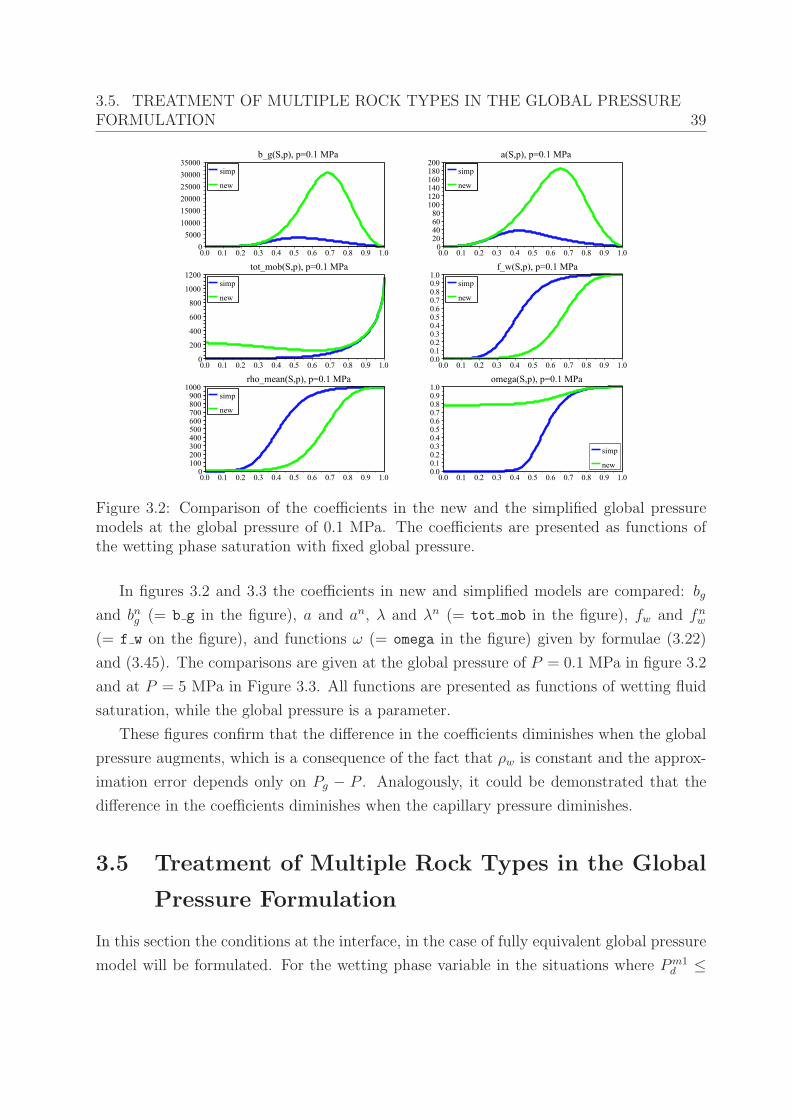
3.5. TREATMENT OF MULTIPLE ROCK TYPES IN THE GLOBAL PRESSUREFORMULATION 39
Figure 3.2: Comparison of the coefficients in the new and the simplified global pressuremodels at the global pressure of 0.1 MPa. The coefficients are presented as functions ofthe wetting phase saturation with fixed global pressure.
In figures 3.2 and 3.3 the coefficients in new and simplified models are compared: bg
and bng (= b g in the figure), a and an, λ and λn (= tot mob in the figure), fw and fnw
(= f w on the figure), and functions ω (= omega in the figure) given by formulae (3.22)
and (3.45). The comparisons are given at the global pressure of P = 0.1 MPa in figure 3.2
and at P = 5 MPa in Figure 3.3. All functions are presented as functions of wetting fluid
saturation, while the global pressure is a parameter.
These figures confirm that the difference in the coefficients diminishes when the global
pressure augments, which is a consequence of the fact that ρw is constant and the approx-
imation error depends only on Pg − P . Analogously, it could be demonstrated that the
difference in the coefficients diminishes when the capillary pressure diminishes.
3.5 Treatment of Multiple Rock Types in the Global
Pressure Formulation
In this section the conditions at the interface, in the case of fully equivalent global pressure
model will be formulated. For the wetting phase variable in the situations where Pm1d ≤
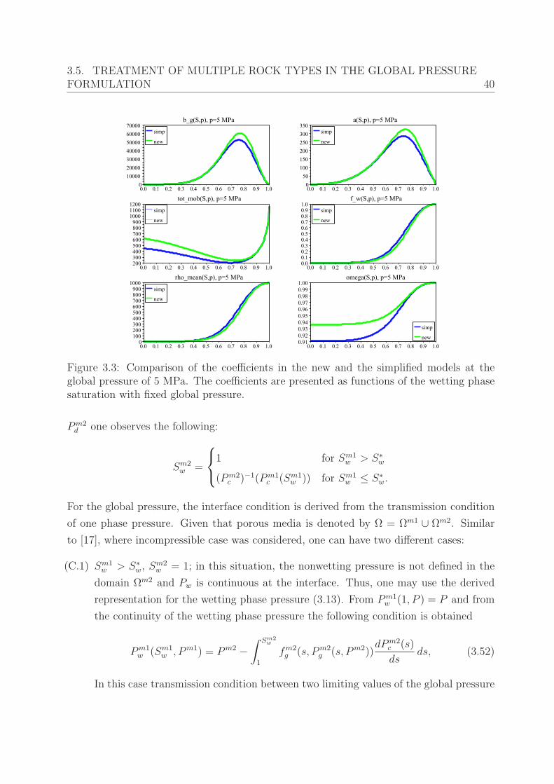
3.5. TREATMENT OF MULTIPLE ROCK TYPES IN THE GLOBAL PRESSUREFORMULATION 40
Figure 3.3: Comparison of the coefficients in the new and the simplified models at theglobal pressure of 5 MPa. The coefficients are presented as functions of the wetting phasesaturation with fixed global pressure.
Pm2d one observes the following:
Sm2w =
1 for Sm1w > S∗
w
(Pm2c )−1(Pm1
c (Sm1w )) for Sm1
w ≤ S∗
w.
For the global pressure, the interface condition is derived from the transmission condition
of one phase pressure. Given that porous media is denoted by Ω = Ωm1 ∪ Ωm2. Similar
to [17], where incompressible case was considered, one can have two different cases:
(C.1) Sm1w > S∗
w, Sm2w = 1; in this situation, the nonwetting pressure is not defined in the
domain Ωm2 and Pw is continuous at the interface. Thus, one may use the derived
representation for the wetting phase pressure (3.13). From Pm1w (1, P ) = P and from
the continuity of the wetting phase pressure the following condition is obtained
Pm1w (Sm1
w , Pm1) = Pm2 −∫ Sm2
w
1
fm2g (s, Pm2
g (s, Pm2))dPm2
c (s)
dsds, (3.52)
In this case transmission condition between two limiting values of the global pressure
3.5. TREATMENT OF MULTIPLE ROCK TYPES IN THE GLOBAL PRESSUREFORMULATION 41
is described by the nonlinear equation (3.52). In fact, the following applies:
Pm2 = Pm1w (Sm1
w , Pm1). (3.53)
From given Pm1 and Sm1w the Pm2 can be calculated by (3.52)). In reverse, for given
Pm2 and Sm1w one may calculate Pm1 by solving the nonlinear equation (3.53), for
which the solution is defined since the derivative of the wetting phase pressure over
global pressure is strictly positive.
(C.2) Sm1w ≤ S∗
w, Pm1c (Sm1
w ) = Pm2c (Sm2
w ); here the phase pressures are continuous across
the interface, and in the same way like described in [17] one can use the continuity
of the nonwetting phase pressure to obtain
Pm1g (Sm1
w , Pm1) = Pm2g (Sm2
w , Pm2). (3.54)
In this case, when Sm1w and Sm2
w are given, one obtains Pm2 from any given Pm1 by
solving the nonlinear equation
Pm1g = Pm2
g (Sm2w , Pm2), (3.55)
whose solution is well defined since the partial derivative of the nonwetting pressure
over global pressure is strictly positive. Also, for any given Pm2 one may calculate
Pm1 from the nonlinear equation
Pm1g (Sm1
w , Pm1) = Pm2g .
Remark 3.5. Note that in the case of the van Genuchten functions the case (C.2) always
applies.
Remark 3.6. In the situation when the interface separates multiple rock types, the condi-
tions described above are assumed for each pair of materials containing the same interface
Remark 3.7. The same transmission conditions can be applied in the case of simplified
model, in the range of its validity.
3.6. CONCLUSION 42
3.6 Conclusion
A new immiscible compressible two-phase flow model (3.23)–(3.25) is developed. The
model is based on the global pressure concept which is fully equivalent to the original
phase equation formulation (2.20), (2.21). This model is compared to the simplified frac-
tional flow model presented in section 3.3. A comparison of the coefficients in the two
models reveals that simplification based on replacing the phase pressures by the global
pressure in calculations of mass densities can safely be used in applications when mean
field pressure is high, capillary pressure is relatively small and if the wetting phase is not
strongly compressible. This is the case in oil-gas systems. In hydro-geological applica-
tions, where capillary pressures may be elevated with respect to mean field pressure, this
approximation can introduce unacceptably large errors, especially in predicting total mass
of the nonwetting phase. These conclusions are confirmed by numerical simulation in the
following chapter.
43
Chapter 4
Numerical Simulations
This chapter is devoted to the numerical simulations of the fully equivalent global pressure
model. At first the numerical scheme is presented. Special attention is paid to the treat-
ment of the heterogeneities and association of the numerical scheme and the transmission
conditions. Furthermore, three monodimensional test cases are presented [52].
The first test case is related to the flow of gas and water in heterogeneous porous
media with no discontinuities of the capillary pressure at the initial time. The second test
case is the benchmark BO-BG, French acronym of Engineered Barrier Geological Barrier,
which was proposed by the French research group MoMaS (http://www.gdrmomas.org/) to
advance numerical methods used in the simulations concerning the gas migration through
engineered and geological barriers for the deep repository of radioactive waste. In this test
the initial capillary pressure is taken to be discontinuous. The third test case presents the
situations that include the capillary pressure curves with nonzero entry pressure. During
this chapter, most of the time the subscript w referring to the wetting phase saturation is
omitted, and only S is used.
4.1 A Finite Volume Scheme
In this section, a vertex-centered finite volume method applied to the system of equations
(3.23)-(3.25) for the one-dimensional case is presented.
4.1. A FINITE VOLUME SCHEME 44
4.1.1 Basic Notation
The equations (3.24)-(3.25) are solved on a finite time interval J = ]0, T [, and in a finite
spatial domain I = ]a, b[. In order to present the discretization, the following notation is
applied, similar to the one presented in [1, 2, 5]:
(N.1) Let
t0 < t1 < . . . < tNT
be the discretization of the time domain and by Jk =
[tk, tk+1[ denote the k-level time interval. The time step is: tk = tk+1 − tk, k =
0, 1, . . . , NT − 1.
(N.2) Let x0 < x1 < . . . < xNx be the discretization of the spatial domain where:
Ei+ 12
:= [xi, xi+1] , i = 0, 1, . . . , Nx − 1, as shown in the figure 4.1 and set xi =
|Ei+ 12| = xi+1 − xi, i = 0, 1, . . . , Nx − 1.
(N.4) Control volumes are defined as follows: for each i ∈ 0, 1, . . . , Nx − 1 denote the
center of the element Ei+ 12
by xi+ 12
:= xi+xi+1
2, and set x
−12
= x0 and xNx+ 12
= xNx.
For i = 0, . . . , Nx, the control volume is defined as Vi = [xi− 12, xi+ 1
2]. By setting
hi = |Vi| = xi+ 12− xi− 1
2, i = 0, 1, 2 . . . , Nx, one obtains h0 = ∆x0
2, hNx
=∆xNx−1
2
and hi = ∆xi−1+∆xi
2, i = 0, 1, . . . , Nx − 1.
(N.5) Let φj, j = 0, . . . , Nx (φj(xj) = 1) be the set of P1 base functions. The approxima-
tions
S(x, t) =N∑
j=0
Sj(t)φj(x), P (x, t) =N∑
j=0
Pj(t)φj(x)
are required. The approximations of S(xi, tk) and P (xi, tk), are denoted by Ski and
P ki .
(N.6) For the porosity, Φ ∈ L∞(I) one sets: φi = 1hi
∫
ViΦ(x) dx.
(N.7) The permeability is scalar function of the space and it is assumed to be constant on
the element: Ki+ 12
= K∣
∣
Ei+1
2
A special care has to be taken when spatial mesh creation is performed in the situations
with multiple rock types. As explained in the previous chapters, in each rock type the
rock properties differ. Relative permeability and the capillary pressure functions may be
different for each rock type as well.

4.1. A FINITE VOLUME SCHEME 45
If the spatial domain in one dimension is divided into Nm parts, and each part of the
domain is related to a certain rock type, there are Nm − 1 interfaces. Every interface point
is set to be an element of the spatial mesh x0 < x1 < . . . < xNx. The other nodes of the
spatial mesh can be chosen arbitrarily.
For the sake of simplicity and without loss of generality, the numerical scheme will be
presented for the situation of the two rock types. A higher number of materials does not
influence the presentation of the treatment of heterogeneity employed in this thesis. In
the case with higher dimensions, the situation complicates further. In the following, it is
assumed that the spatial domain is divided into two parts, one related to the material m1
and the other related to the material m2, as is presented in the figure 4.1.
E
Figure 4.1: Spatial mesh in one-dimensional case
Let Im1 ∪ Im2 = I and the interface node is set to be xδ = Im1 ∩ Im2, for an index
δ ∈ 0, 1, . . . , NxThe superscript n in the definition of the coefficients (3.16)-(3.20) is omitted to further
simplify notation. Also the subscript t used previously in the notation of the total flux, is
omitted. For the same reason the following functions are introduced (either m = m1 or
m = m2):
Mm := Mm(S, P ) := ρw(Pmw (S, P ))S + ρg(P
mg (S, P ))(1 − S)
Nm := N(S, p) := ρw(Pmw (S, p))S.
χm(S, P ) := λm(S, P )ωm(S, P )
γ(S, P ) := −α(S, P ), so that a(S, P ) = γ(S, P )P ′
c(S).
4.1. A FINITE VOLUME SCHEME 46
The equations (3.23)-(3.25) (with neglected gravity term) rewritten in one-dimensional
case are:
Φ∂
∂t(Mm(S, P ))) − ∂
∂x
(
χm(S, P )K∂P
∂x
)
= Fw + Fg (4.1)
Qm = −χm(S, P )K∂P
∂x(4.2)
Φ∂
∂t(Nm(S, P )) +
∂
∂x(Qmfm
w (S, p)) − ∂
∂x
(
γm(S, P )K∂Pm
c (S)
∂x
)
= Fw (4.3)
At initial time, either the global pressure, the saturation or the phase pressures are
given. A set of boundary conditions of diverse types can be given.
As already mentioned, in the chapter 3, the saturation and the global pressure are
generally discontinuous at the interface point. Therefore, it is worthwhile to explain the
meaning and use of the global unknowns Skδ and P k
δ , at the interface node xδ.
4.1.2 Interface Conditions
The values Skδ and P k
δ are solutions of the nonlinear problem for each time step. These are
considered to be the representative values of the true limit values defined by the elements.
The index k is omitted below to simplify the notation.
There are several ways of defining these global unknowns. At first consider the sat-
uration variable and recall that at the interface point the following equality has to be
satisfied:
Pm1c (Sm1
δ ) = Pm2c (Sm2
δ ), (4.4)
if one assumes that Pm1c (1) = Pm2
c (1) = 0, otherwise extended capillary pressure condition
needs to be satisfied. Here Pm1c (Pm2
c ) is the capillary pressure defined for the material m1
( material m2), and Sm1δ (Sm2
δ ) are respective limiting saturations. When the wetting phase
saturation is the primary unknown of the system, in the computation by the elements
the true limit values of the saturation need to be used. This also guarantees that during
calculation one actually always works with the correct capillary pressure at the interface
node xδ.
The unknown value Sδ at the interface node xδ can be chosen in several ways. For
instance, it can be taken as Sδ = f(Sm1δ , Sm2
δ ), where f an invertible function in every
4.1. A FINITE VOLUME SCHEME 47
variable. The simplest approach, however, is to choose Sδ = Sm1δ or Sδ = Sm2
δ .
The situation with the global pressure is similar. The global pressure will generally be
discontinuous at the interface point. The choice of Pδ can be done in several ways, and the
simplest approach is to choose Pδ = Pm1δ or Pδ = Pm2
δ , and then use the continuity of the
nonwetting phase pressure:
Pm1g (Sm1
δ , Pm1δ ) = Pm2
g (Sm2δ , Pm2
δ ) (4.5)
at the interface, in order to obtain the other limiting value, depending on which part of
the domain the calculation is done.
This is applicable if the nonwetting phase is mobile at the interface, otherwise one needs
to use the continuity of the wetting phase pressure.
Remark 4.1. In the simulations where the entry pressure is present (e.g. Brooks and
Corey capillary pressure), the choice of the unknown Sδ is more restrictive. It has to be
taken equal to the limiting saturation of the material which is related to the smaller “entry
pressure” [17,56]. If this is the region Im1, the extended capillary pressure condition (2.50)
to calculate the saturation Sm2δ is used.
4.1.3 Numerical Scheme Presentation
For any function f(S, P ) we define:
fm,k
i+ 12
= fm(Ski+ 1
2, P k
i+ 12).
The following notation is used:
Ski+ 1
2=Sk
i + Ski+1
2, P k
i+ 12
=P k
i + P ki+1
2.
4.1. A FINITE VOLUME SCHEME 48
At first, the system (4.1)-(4.3) is integrated over the set Vi × Jk to obtain:
∫
Vi
Φ(
Mm(Sk+1, P k+1) −Mm(Sk, P k)))
dx−∫
Jk
∑
j=±12
(2j)χmi+jKi+j
(
∂P
∂x
)
i+j
dt
= |Vi|(Fw,i + Fg,i)∫
Vi
Φ(
Nm(Sk+1, P k+1) −Nm(Sk, P k)))
dx+
∫
Jk
∑
j=±12
(2j)Qmi+jf
m,upw,i+j dt
=
∫
Jk
∑
j=±12
(2j)γmi+jKi+j
(
∂Pmc (S)
∂x
)
i+j
dt
+ |Vi|Fw,i
Now, various approximations can be used:
(
∂P
∂x
)
i+ 12
=Pi+1 − Pi
∆xi
,
(
∂Pmc (S)
∂x
)
i+ 12
=Pm
c (Si+1) − Pmc (Si)
∆xi
.
On the left side of the equations the mass lumping is applied. The following equations
are obtained:
ΦihiMm,k+1
i −Mm,ki
∆tk= Rk+1
p,i (4.6)
ΦihiNm,k+1
i −Nm,ki
∆tk= Rk+1
S,i . (4.7)
The following notation is introduced:
Ti+1/2 :=Ki+1/2
xi
, i = 0, 1, 2 . . . , Nx − 1.
For i = 1, 2, . . . , Nx − 1, the right hand side of the (4.6) is
Rk+1p,i =
∑
j=±12
χm,k+1i+j Ti+j(P
k+1i+2j − P i
i ) + |Vi|(Fg,i + Fw,i). (4.8)
The total velocity for j = ±12
is
Qm,k+1i+j = −χm,k+1
i+j Ti+j(Pk+1i+2j − P k+1
i )
4.1. A FINITE VOLUME SCHEME 49
where m = m1 or m = m2.
For i = 1, 2, . . . Nx − 1
Rk+1S,i =
∑
j=±12
γm,k+1i+j Ti+j(P
mc (Sk+1
i+2j) − Pmc (Sk+1
i )) (4.9)
−∑
j=±12
(2j)Qm,k+1i+j (fm
w )m,up,k+1i+j + |Vi|(Fw,i), (4.10)
where, if the type of problem requires, the following upwind procedure is applied:
fm,up,k+1
w,i+ 12
=
fmw (Sk+1
i , P k+1i ) for Qk+1
i+ 12
≥ 0
fmw (Sk+1
i+1 , Pk+1i+1 ) for Qk+1
i+ 12
< 0.
Otherwise, the standard expression for Rk+1S,i is used:
Rk+1S,i =
∑
j=±12
γm,k+1i+j Ti+j(P
mc (Sk+1
i+2j) − Pmc (Sk+1
i )) (4.11)
−∑
j=±12
Qm,k+1i+j (fm
w )m,k+1i+j + |Vi|(Fw,i). (4.12)
The terms Rk+1S,0 , R
k+1p,0 , R
k+1p,Nx
, Rk+1S,Nx
depend on the imposed boundary conditions.
Notes on the Discretization of Boundary Conditions
For simplicity it is assumed Fw = 0 Fg = 0. If setting the total flux Q = Qin, and flux of
wetting phase Qw = Qw,in on the left boundary, one obtains:
Rk+1p,0 = χm1,k+1
12
T 12(P k+1
1 − P k+10 ) +Qin
Rk+1S,0 = γm,k+1
12
T 12(Pm
c (Sk+11 ) − Pm
c (Sk+10 )) −Qm,k+1
12
(fw)m,up,k+112
+Qw,in.
If setting the total flux Q = Qout, and Qw = Qw,out on the right boundary, one obtains:
Rk+1p,Nx
= −χm2,k+1
Nx−12
TNx−12(P k+1
Nx− P k+1
Nx−1) −Qout
4.1. A FINITE VOLUME SCHEME 50
Rk+1S,Nx
= −γm,k+1
Nx−12
TNx−12(Pm
c (Sk+1Nx
) − Pmc (Sk+1
Nx−1)) +Qm,k+1
Nx−12
(fw)m,up,k+1
Nx−12
−Qw,out
Remark 4.2. If fluxes are set to be zero at the boundary (Q = 0, Qw = 0) the expressions
(4.8) and (4.10) can also be used for i = 0 and for i = Nx if:
P k−1 = P k
0 Qk−
12
:= QkNx+ 1
2= 0
Pm1c (Sk
−1) = Pm1c (Sk
0 ) Pm2c (Sk
Nx+1) = Pm2c (Sk
Nx).
For Dirichlet boundary conditions S = Sin and P = Pin on the left part of the boundary
one obtains:
Rk+1p,0 = P − Pin, Mm,k+1
0 −Mm,k0 ≡ 0.
Rk+1S,0 = Sk+1
0 − Sin, Nm,k+10 −Nm,k
0 ≡ 0.
Similar expressions, are obtained for setting Dirichlet boundary conditions on the right
part of the boundary.
Commonly, Neumann boundary condition for the saturation is used. A case when at
the right boundary it is taken ∂S∂x
∣
∣
x=xNx
= 0 is discussed in the following.
Note that for xNxone obtains
ΦNxhNx
Mm2,k+1Nx
−Mm2,kNx
∆t= −Qm2,k+1
out − χk+1
i−Nx2
TNx−12(P k+1
Nx− P k+1
Nx−1),
which provides a way to calculate Qn+1out :
Qm2,n+1out = −ΦNx
hNx
Mm2,k+1Nx
−Mm2,kNx
∆t− χm2,k+1
i−Nx2
Ti− 12(P k+1
Nx− P k+1
Nx−1)
One can set an upwind value at the node xNxas follows:
fup,n+1w,out =
f((Sk+1
Nx−1+Sn+1Nx
)
2,
(P k+1Nx−1+Pout)
2) for Qk+1
out ≥ 0
f(Sn+1Nx
, Pout) for Qn+1out < 0
and in that case equation (4.10) for Rk+1S,Nx
can be used.
4.1. A FINITE VOLUME SCHEME 51
Nonlinear Equations
Notice that at each time step a nonlinear problem is obtained. This type of problem
may be solved by the Picard iterations or by the Newton method. In order to use the
Newton method, one needs to know how to form a residual and a Jacobian at the previous
iteration. While those calculations are done, special attention needs to be paid to the
interface node. Considering that all the calculations are performed locally at the element
E, it is worthwhile to have an insight into the local calculations. A brief explanation is
given in the following subsection.
4.1.4 Local Calculations
All the functions used in the discretization belong to the material where the current element
is positioned. Therefore, material index will be omitted in this section. Considering that
the time index is constant in the scope of this discussion, it is omitted as well. The local
calculations are presented for the situation when phase fluxes are set to be zero at the
boundary. For the simplicity, it is assumed that Pc(1) = 0.
Local Residuals
Denote the local element by E = [x0, x1]. The global unknowns are: P0, P1, S0, S1. In
general, assume that local values S+0 , S
−
1 depend on the values S0 and S1 respectively.
Assume, as well, that P+0 depends on S0 and P0, and P−
1 depends on P1 and S1.
In the local calculation, the local values S+0 , P
+0 , S
−
1 , P−
1 will be used. As discussed in
the previous section, if calculations are performed at the interface node, one needs to know
the limit values of saturation and global pressure. These are obtained from the global
unknown value from the previous iteration. Consider the simplest example:
• If the global unknown at the node xδ is set to be equal to the left limiting saturation,
then S−
1 = S1 is always valid. However, at the point x0 the calculations have to be
performed more carefully. the following is set:
S+0 =
S0 if x0 6= xδ
(Pm2c )−1(Pm1
c (S0)) for x0 = xδ
.
• If the global unknown at the node xδ is set to be equal to the left limiting pressure,
then P−
1 = P1 and at x0 calculation have to be performed more carefully. Assuming
4.1. A FINITE VOLUME SCHEME 52
S+0 is already calculated, the following is set:
P+0 =
P0 if x0 6= xδ
solution of Pm1g (S0, P0) = Pm2
g (S+0 , P
+0 ) if x0 = xδ
.
The permeability K is constant on the element. One sets:
P 12
=P+
0 + P−
1
2, S 1
2=S+
0 + S−
1
2, dx = x1 − x0, T =
K
dx,
and now follows:
Rp,0 = χ(S 12, P 1
2)T (P−
1 − P+0 )
Rp,1 = −χ(S 12, P 1
2)T (P−
1 − P+0 ).
Also, the following equalities are obtained:
RS,0 = γ(S 12, P 1
2)T (Pc(S
−
1 ) − Pc(S+0 )) −Q 1
2fup
w
RS,1 = −γ(S 12, p 1
2)T (Pc(S
−
1 ) − Pc(S+0 )) +Q 1
2fup
w
where
Q 12
= −χ(S 12, P 1
2)T (P−
1 − P+0 ), fup
w =
fw(S+0 , P
+0 ) for Q 1
2≥ 0
fw(S−
1 , P−
1 ) for Q 12< 0
.
Local Jacobian
To form the Jacobian, one needs to know the derivatives
dS+0
dS0
(S0),dS−
1
dS1
(S1),∂P+
0
∂S0
(S0, P0),∂P+
0
∂P0
(S0, P0),∂P−
1
∂S1
(S1, P1),∂P−
1
∂P1
(S1, P1).
If x0 is not the interface node these values are calculated as usual. The following applies:
S+0 = S0,
dS+0
dS0
= 1, P+0 = P0,
∂P+0
∂S0
= 0,∂P+
0
∂P0
= 1.
The same situation is when x1 is not the interface node.
4.1. A FINITE VOLUME SCHEME 53
Remark 4.3. To further simplify the notation, the function arguments will be omitted. By
setting the global unknown at the interface equal to the left limiting saturation (pressure),
one obtains:
S−
1 = S1,∂S−
1
∂S1
= 1, P−
1 = P1,∂P−
1
∂S1
= 0,∂P−
1
∂P1
= 1.
From the transmission conditions (4.4) and (4.5) one obtains the following:
∂S+0
∂S0
=
1 if x0 6= xδ(
dP m1c (S0)dS
)
/(
dP m2c (S+
0 )
dS
)
for x0 = xδ
∂P+0
∂S0
=
0 if x0 6= xδ
∂Pm1g (S0,P0)
∂S0−
∂Pm2g (S+
0 ,P+0 )
∂S
∂S+0
∂S
ωm2(S+0 ,P+
0 )for x0 = xδ
∂P+0
∂P0
=
1 if x0 6= xδ
ωm1(S0,P0)
ωm2(S+0 ,P+
0 )for x0 = xδ
.
Note that when the unknowns at the interface node are selected differently, the above deriva-
tives have to be calculated accordingly.
It follows:
DPRP =
[
∂P0RP,0 ∂P1RP,0
∂P0Rp,1 ∂P1RP,1
]
= T
[
α1 β1
−α1 −β1
]
where
α1 =1
2∂Pχ(S 1
2, P 1
2)∂P+
0
∂P0
(P−
1 − P+0 ) − χ(S 1
2, P 1
2)∂P+
0
∂P0
β1 =1
2∂Pχ(S 1
2, P 1
2)∂P−
1
∂P1
(P−
1 − P+0 ) + χ(S 1
2, P 1
2)∂P−
1
∂P1
.
One obtains
DSRp =
[
∂S0RP,0 ∂S1RP,0
∂S0RP,1 ∂S1RP,1
]
= T
[
α2 β2
−α2 −β2
]
4.1. A FINITE VOLUME SCHEME 54
where
α2 =1
2
(
∂Sχ(S 12, P 1
2)∂S+
0
∂S0
+ ∂Pχ(S 12, p 1
2)∂P+
0
∂S0
)
(P−
1 − P+0 ) − χ(S 1
2, P 1
2)∂P+
0
∂S0
β2 =1
2
(
∂Sχ(S 12, P 1
2)∂S−
1
∂S1
+ ∂Pχ(S 12, P 1
2)∂P−
1
∂S1
)
(P−
1 − P+0 ) + χ(S 1
2, P 1
2)∂P−
1
∂S1
.
Total velocity derivatives are
∂Q 12
∂S0
= −Tα2
∂Q 12
∂S1
= −Tβ2
∂Q 12
∂P0
= −Tα1
∂Q 12
∂P1
= −Tβ1.
Upwind flux derivatives are
∂S0fupw =
∂Sfw(S+0 , P
+0 )
∂S+0
∂S0+ ∂Pfw(S+
0 , P+0 )
∂P+0
∂S0for Q 1
2≥ 0
0 for Q 12< 0
∂P0fupw =
∂Pfw(S+0 , P
+0 )
∂P+0
∂P0for Q 1
2≥ 0
0 for Q 12< 0
∂S1fupw =
0 for Q 12≥ 0
∂Sfw(S−
1 , P−
1 )∂S−
1
∂S1+ ∂Pf(S−
1 , P−
1 )∂P−
1
∂S1for Q 1
2< 0
∂P1fupw =
0 for Q 12≥ 0
∂pf(S−
1 , P−
1 )∂P−
1
∂P1for Q 1
2< 0
.
Convective flux derivatives are
∂
∂S0
(Q 12fup
w ) =∂Q 1
2
∂S0
fupw +Q 1
2
∂fupw
∂S0
= −Tα2fupw + max(Q 1
2, 0)∂S0f
upw
∂
∂S1
(Q 12fup
w ) =∂Q 1
2
∂S1
fupw +Q 1
2
∂fupw
∂S1
= −Tβ2fupw + min(Q 1
2, 0)∂S1f
upw
∂
∂P0
(Q 12fup
w ) =∂Q 1
2
∂P0
fupw +Q 1
2
∂fupw
∂P0
= −Tα1fupw + max(Q 1
2, 0)∂P0f
upw
∂
∂P1
(Q 12fup
w ) =∂Q 1
2
∂P1
fupw +Q 1
2
∂fupw
∂p1
= −Tβ1fupw + min(Q 1
2, 0)∂P1f
upw .
4.1. A FINITE VOLUME SCHEME 55
The residual is decomposed as follows:
RS,0 = RdifS,0 +Rcon
S,0 , RS,1 = RdifS,1 +Rcon
S,1
where
RdifS,0 = γ(S 1
2, P 1
2)T (Pc(S
−
1 ) − Pc(S+0 )), Rcon
S,0 = −Q 12fup
w
RdifS,1 = −γ(S 1
2, P 1
2)T (Pc(S
−
1 ) − Pc(S+0 )), Rcon
S,1 = Q 12fup
w ,
so it follows
DSRS =
[
∂S0RS,0 ∂S1RS,0
∂S0RS,1 ∂S1RS,1
]
= DSRdifS +DSR
conS
DpRS =
[
∂P0RS,0 ∂P1RS,0
∂P0RS,1 ∂P1RS,1
]
= DPRdifS +DPR
conS .
Using the notation γ 12
= γ(S 12, P 1
2) and ∂Pγ 1
2= ∂Pγ(S 1
2, P 1
2) one obtains:
DSRdifS =
[
∂S0RdifS,0 ∂S1R
difS,0
∂S0RdifS,1 ∂S1R
difS,1
]
= T
[
α3 β3
−α3 −β3
]
,
where
α3 =
(
1
2∂Sγ 1
2
∂S+0
∂S0
+1
2∂Pγ 1
2
∂P+0
∂S0
)
(Pc(S−
1 ) − Pc(S+0 )) − γ 1
2P ′
c(S+0 )∂S+
0
∂S0
β3 =
(
1
2∂Sγ 1
2
∂S−
1
∂S1
+1
2∂Pγ 1
2
∂P−
1
∂S1
)
(Pc(S−
1 ) − Pc(S+0 )) + γ 1
2P ′
c(S−
1 )∂S−
1
∂S1
.
It follows:
DPRdifS =
[
∂P0RdifS,0 ∂P1R
difS,0
∂P0RdifS,1 ∂P1R
difS,1
]
= T
[
α4 β4
−α4 −β4
]
4.1. A FINITE VOLUME SCHEME 56
where
α4 =1
2∂Pγ 1
2
∂P+0
∂P0
(Pc(S−
1 ) − Pc(S+0 ))
β4 =1
2∂Pγ 1
2
∂P−
1
∂P1
(Pc(S−
1 ) − Pc(S+0 )).
For the convective part of the Jacobian is valid:
DSRconS =
[
−∂S0(Q 12fup
w ) −∂S1(Q 12fup
w )
∂S0(Q 12fup
w ) ∂S1(Q 12fup
w )
]
, DPRconS =
[
−∂P0(Q 12fup
w ) −∂P1(Q 12fup
w )
∂P0(Q 12fup
w ) ∂P1(Q 12fup
w )
]
.
Mass Residual and Jacobian
In calculations by elements one has to calculate
M0 = ρw(S+0 , P
+0 )S+
0 + ρg(S+0 , P
+0 )(1 − S+
0 )
N0 = ρw(S+0 , P
+0 )S+
0 ,
M1 = ρw(S−
1 , P−
1 )S−
1 + ρg(S−
1 , P−
1 )(1 − S−
1 )
N1 = ρw(S−
1 , P−
1 )S−
1 .
To form the Jacobian, one requires derivatives of the functions M and N :
∂M(S+0 , P
+0 )
∂P0
= ∂pM(S+0 , P
+0 )∂P+
0
∂P0
∂M(S−
1 , P−
1 )
∂P1
= ∂pM(S−
1 , P−
1 )∂P−
1
∂P1
∂M(S+0 , P
+0 )
∂S0
= ∂SM(S+0 , P
+0 )∂S+
0
∂S0
+ ∂pM(S+0 , P
+0 )∂P+
0
∂S0
∂M(S−
1 , P−
1 )
∂S1
= ∂SM(S−
1 , P−
1 )∂S−
1
∂S1
+ ∂pM(S−
1 , P−
1 )∂P−
1
∂S1
.
For the function N , the calculation is analogous.
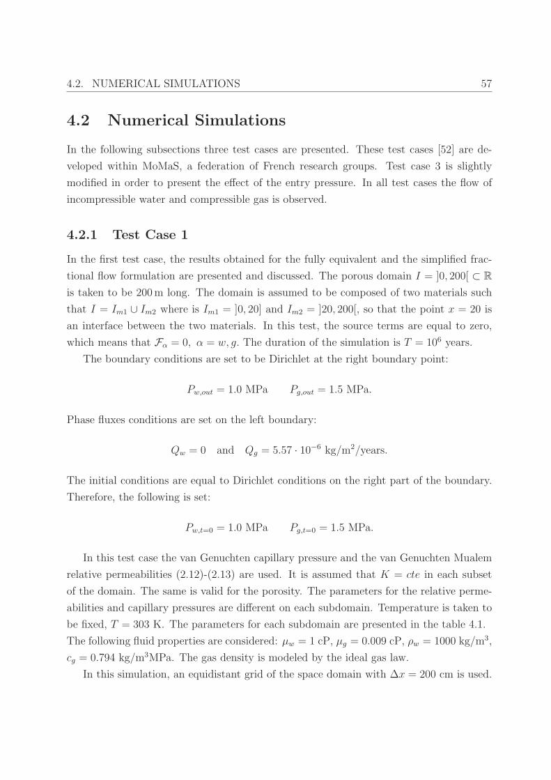
4.2. NUMERICAL SIMULATIONS 57
4.2 Numerical Simulations
In the following subsections three test cases are presented. These test cases [52] are de-
veloped within MoMaS, a federation of French research groups. Test case 3 is slightly
modified in order to present the effect of the entry pressure. In all test cases the flow of
incompressible water and compressible gas is observed.
4.2.1 Test Case 1
In the first test case, the results obtained for the fully equivalent and the simplified frac-
tional flow formulation are presented and discussed. The porous domain I = ]0, 200[ ⊂ R
is taken to be 200 m long. The domain is assumed to be composed of two materials such
that I = Im1 ∪ Im2 where is Im1 = ]0, 20] and Im2 = ]20, 200[, so that the point x = 20 is
an interface between the two materials. In this test, the source terms are equal to zero,
which means that Fα = 0, α = w, g. The duration of the simulation is T = 106 years.
The boundary conditions are set to be Dirichlet at the right boundary point:
Pw,out = 1.0 MPa Pg,out = 1.5 MPa.
Phase fluxes conditions are set on the left boundary:
Qw = 0 and Qg = 5.57 · 10−6 kg/m2/years.
The initial conditions are equal to Dirichlet conditions on the right part of the boundary.
Therefore, the following is set:
Pw,t=0 = 1.0 MPa Pg,t=0 = 1.5 MPa.
In this test case the van Genuchten capillary pressure and the van Genuchten Mualem
relative permeabilities (2.12)-(2.13) are used. It is assumed that K = cte in each subset
of the domain. The same is valid for the porosity. The parameters for the relative perme-
abilities and capillary pressures are different on each subdomain. Temperature is taken to
be fixed, T = 303 K. The parameters for each subdomain are presented in the table 4.1.
The following fluid properties are considered: µw = 1 cP, µg = 0.009 cP, ρw = 1000 kg/m3,
cg = 0.794 kg/m3MPa. The gas density is modeled by the ideal gas law.
In this simulation, an equidistant grid of the space domain with ∆x = 200 cm is used.
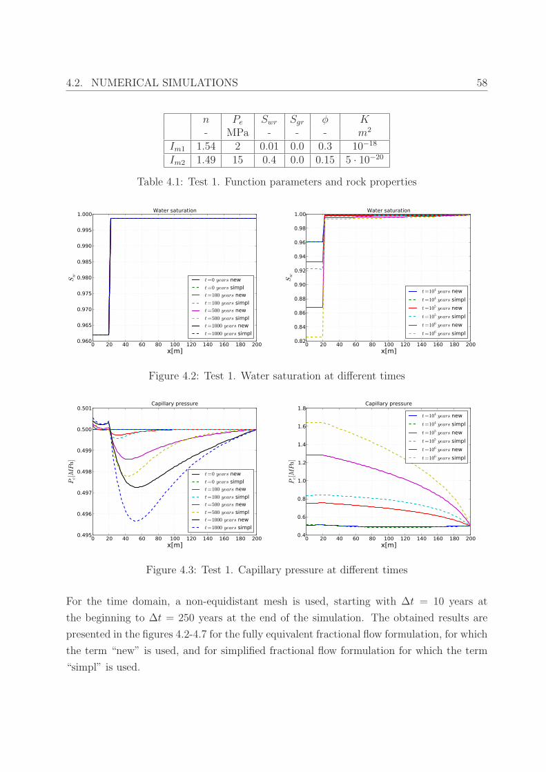
4.2. NUMERICAL SIMULATIONS 58
n Pe Swr Sgr φ K- MPa - - - m2
Im1 1.54 2 0.01 0.0 0.3 10−18
Im2 1.49 15 0.4 0.0 0.15 5 · 10−20
Table 4.1: Test 1. Function parameters and rock properties
0 20 40 60 80 100 120 140 160 180 200x[m]
0.960
0.965
0.970
0.975
0.980
0.985
0.990
0.995
1.000
Sw
Water saturation
t=0 years new
t=0 years simplt=100 years new
t=100 years simplt=500 years new
t=500 years simplt=1000 years new
t=1000 years simpl
0 20 40 60 80 100 120 140 160 180 200x[m]
0.82
0.84
0.86
0.88
0.90
0.92
0.94
0.96
0.98
1.00
Sw
Water saturation
t=104 years new
t=104 years simpl
t=105 years new
t=105 years simpl
t=106 years new
t=106 years simpl
Figure 4.2: Test 1. Water saturation at different times
0 20 40 60 80 100 120 140 160 180 200x[m]
0.495
0.496
0.497
0.498
0.499
0.500
0.501
Pc[MPa]
Capillary pressure
t=0 years new
t=0 years simplt=100 years new
t=100 years simplt=500 years new
t=500 years simplt=1000 years new
t=1000 years simpl
0 20 40 60 80 100 120 140 160 180 200x[m]
0.4
0.6
0.8
1.0
1.2
1.4
1.6
1.8
Pc[MPa]
Capillary pressure
t=104 years new
t=104 years simpl
t=105 years new
t=105 years simpl
t=106 years new
t=106 years simpl
Figure 4.3: Test 1. Capillary pressure at different times
For the time domain, a non-equidistant mesh is used, starting with ∆t = 10 years at
the beginning to ∆t = 250 years at the end of the simulation. The obtained results are
presented in the figures 4.2-4.7 for the fully equivalent fractional flow formulation, for which
the term “new” is used, and for simplified fractional flow formulation for which the term
“simpl” is used.
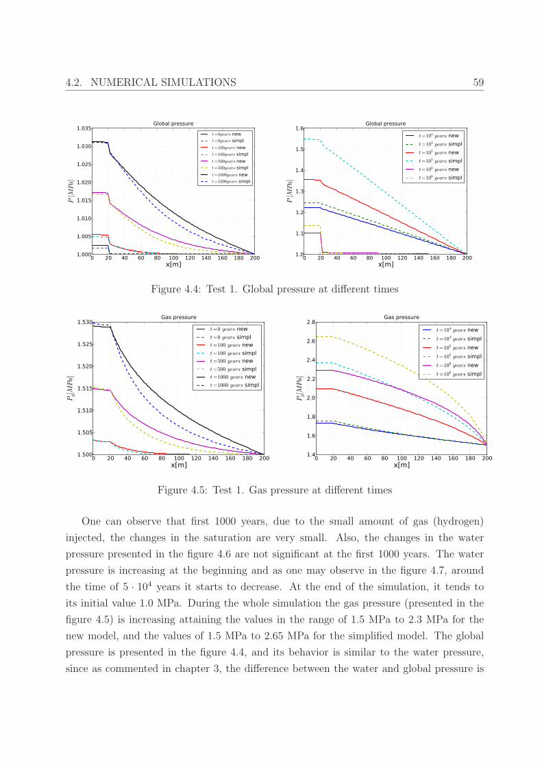
4.2. NUMERICAL SIMULATIONS 59
0 20 40 60 80 100 120 140 160 180 200x[m]
1.000
1.005
1.010
1.015
1.020
1.025
1.030
1.035
P[M
Pa]
Global pressure
t=0years new
t=0years simpl
t=100years new
t=100years simpl
t=500years new
t=500years simpl
t=1000years new
t=1000years simpl
0 20 40 60 80 100 120 140 160 180 200x[m]
1.0
1.1
1.2
1.3
1.4
1.5
1.6
P[M
Pa]
Global pressure
t=104 years new
t=104 years simpl
t=105 years new
t=105 years simpl
t=106 years new
t=106 years simpl
Figure 4.4: Test 1. Global pressure at different times
0 20 40 60 80 100 120 140 160 180 200x[m]
1.500
1.505
1.510
1.515
1.520
1.525
1.530
Pg[MPa]
Gas pressure
t=0 years new
t=0 years simplt=100 years new
t=100 years simplt=500 years new
t=500 years simplt=1000 years new
t=1000 years simpl
0 20 40 60 80 100 120 140 160 180 200x[m]
1.4
1.6
1.8
2.0
2.2
2.4
2.6
2.8
Pg[MPa]
Gas pressure
t=104 years new
t=104 years simpl
t=105 years new
t=105 years simpl
t=106 years new
t=106 years simpl
Figure 4.5: Test 1. Gas pressure at different times
One can observe that first 1000 years, due to the small amount of gas (hydrogen)
injected, the changes in the saturation are very small. Also, the changes in the water
pressure presented in the figure 4.6 are not significant at the first 1000 years. The water
pressure is increasing at the beginning and as one may observe in the figure 4.7, around
the time of 5 · 104 years it starts to decrease. At the end of the simulation, it tends to
its initial value 1.0 MPa. During the whole simulation the gas pressure (presented in the
figure 4.5) is increasing attaining the values in the range of 1.5 MPa to 2.3 MPa for the
new model, and the values of 1.5 MPa to 2.65 MPa for the simplified model. The global
pressure is presented in the figure 4.4, and its behavior is similar to the water pressure,
since as commented in chapter 3, the difference between the water and global pressure is
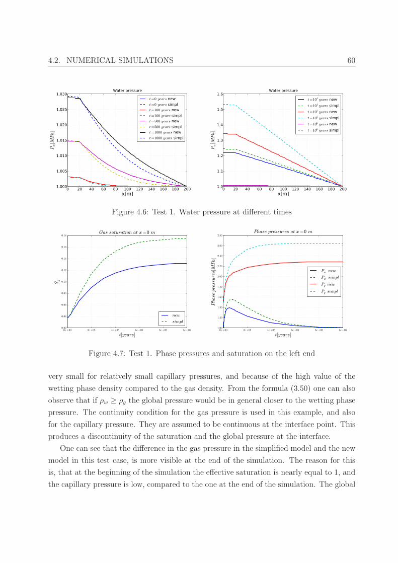
4.2. NUMERICAL SIMULATIONS 60
0 20 40 60 80 100 120 140 160 180 200x[m]
1.000
1.005
1.010
1.015
1.020
1.025
1.030
Pw[M
Pa]
Water pressure
t=0 years new
t=0 years simplt=100 years new
t=100 years simplt=500 years new
t=500 years simplt=1000 years new
t=1000 years simpl
0 20 40 60 80 100 120 140 160 180 200x[m]
1.0
1.1
1.2
1.3
1.4
1.5
1.6
Pw[M
Pa]
Water pressure
t=104 years new
t=104 years simpl
t=105 years new
t=105 years simpl
t=106 years new
t=106 years simpl
Figure 4.6: Test 1. Water pressure at different times
0e+00 2e+05 4e+05 6e+05 8e+05 1e+06
t[years]
0.02
0.04
0.06
0.08
0.10
0.12
0.14
0.16
0.18
Sg
Gas saturation at x=0 m
new
simpl
0e+00 2e+05 4e+05 6e+05 8e+05 1e+06
t[years]
1.00
1.20
1.40
1.60
1.80
2.00
2.20
2.40
2.60
2.80
Phase
pressures[MPa]
Phase pressures at x=0 m
Pw new
Pw simpl
Pg new
Pg simpl
Figure 4.7: Test 1. Phase pressures and saturation on the left end
very small for relatively small capillary pressures, and because of the high value of the
wetting phase density compared to the gas density. From the formula (3.50) one can also
observe that if ρw ≥ ρg the global pressure would be in general closer to the wetting phase
pressure. The continuity condition for the gas pressure is used in this example, and also
for the capillary pressure. They are assumed to be continuous at the interface point. This
produces a discontinuity of the saturation and the global pressure at the interface.
One can see that the difference in the gas pressure in the simplified model and the new
model in this test case, is more visible at the end of the simulation. The reason for this
is, that at the beginning of the simulation the effective saturation is nearly equal to 1, and
the capillary pressure is low, compared to the one at the end of the simulation. The global
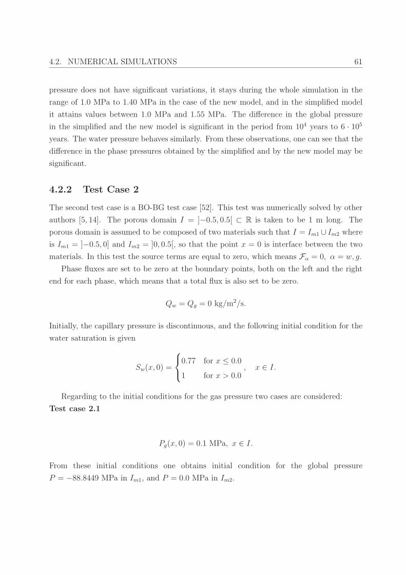
4.2. NUMERICAL SIMULATIONS 61
pressure does not have significant variations, it stays during the whole simulation in the
range of 1.0 MPa to 1.40 MPa in the case of the new model, and in the simplified model
it attains values between 1.0 MPa and 1.55 MPa. The difference in the global pressure
in the simplified and the new model is significant in the period from 104 years to 6 · 105
years. The water pressure behaves similarly. From these observations, one can see that the
difference in the phase pressures obtained by the simplified and by the new model may be
significant.
4.2.2 Test Case 2
The second test case is a BO-BG test case [52]. This test was numerically solved by other
authors [5, 14]. The porous domain I = ]−0.5, 0.5[ ⊂ R is taken to be 1 m long. The
porous domain is assumed to be composed of two materials such that I = Im1 ∪ Im2 where
is Im1 = ]−0.5, 0] and Im2 = ]0, 0.5[, so that the point x = 0 is interface between the two
materials. In this test the source terms are equal to zero, which means Fα = 0, α = w, g.
Phase fluxes are set to be zero at the boundary points, both on the left and the right
end for each phase, which means that a total flux is also set to be zero.
Qw = Qg = 0 kg/m2/s.
Initially, the capillary pressure is discontinuous, and the following initial condition for the
water saturation is given
Sw(x, 0) =
0.77 for x ≤ 0.0
1 for x > 0.0, x ∈ I.
Regarding to the initial conditions for the gas pressure two cases are considered:
Test case 2.1
Pg(x, 0) = 0.1 MPa, x ∈ I.
From these initial conditions one obtains initial condition for the global pressure
P = −88.8449 MPa in Im1, and P = 0.0 MPa in Im2.
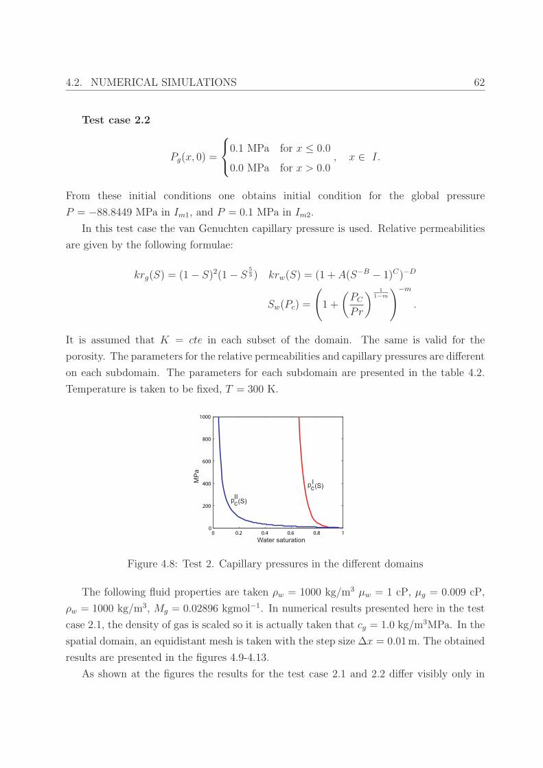
4.2. NUMERICAL SIMULATIONS 62
Test case 2.2
Pg(x, 0) =
0.1 MPa for x ≤ 0.0
0.0 MPa for x > 0.0, x ∈ I.
From these initial conditions one obtains initial condition for the global pressure
P = −88.8449 MPa in Im1, and P = 0.1 MPa in Im2.
In this test case the van Genuchten capillary pressure is used. Relative permeabilities
are given by the following formulae:
krg(S) = (1 − S)2(1 − S53 ) krw(S) = (1 + A(S−B − 1)C)−D
Sw(Pc) =
(
1 +
(
PC
Pr
)1
1−m
)−m
.
It is assumed that K = cte in each subset of the domain. The same is valid for the
porosity. The parameters for the relative permeabilities and capillary pressures are different
on each subdomain. The parameters for each subdomain are presented in the table 4.2.
Temperature is taken to be fixed, T = 300 K.
Figure 4.8: Test 2. Capillary pressures in the different domains
The following fluid properties are taken ρw = 1000 kg/m3 µw = 1 cP, µg = 0.009 cP,
ρw = 1000 kg/m3, Mg = 0.02896 kgmol−1. In numerical results presented here in the test
case 2.1, the density of gas is scaled so it is actually taken that cg = 1.0 kg/m3MPa. In the
spatial domain, an equidistant mesh is taken with the step size ∆x = 0.01 m. The obtained
results are presented in the figures 4.9-4.13.
As shown at the figures the results for the test case 2.1 and 2.2 differ visibly only in
4.2. NUMERICAL SIMULATIONS 63
0.50 0.25 0.00 0.25 0.50x[m]
0.54
0.60
0.66
0.72
0.78
0.84
0.90
0.96
Sw
Water saturation
t=0s
t=10s
t=200s
t=1000s
t=20000s
t=105 s
t=107 s
t=1 year
t=10 years
t=100 years
t=1000 years 0.50 0.25 0.00 0.25 0.50x[m]
0.54
0.60
0.66
0.72
0.78
0.84
0.90
0.96
Sw
Water saturation
t=0s
t=10s
t=200s
t=1000s
t=20000s
t=105 s
t=107 s
t=1 year
t=10 years
t=100 years
t=1000 years
Figure 4.9: Test 2. Water saturation at different times for the test case 2.1 (left) and testcase 2.2 (right)
Pr m A B C D φ KMPa - - - - - - m2
Im1 1.5 0.06 0.25 16.67 1.88 0.5 0.3 10−20
Im2 10 0.412 1.0 2.429 1.176 1.0 0.05 10−19
Table 4.2: Test 2. Function parameters and rock properties
the gas pressures obtained at first 105 s. The right part of the domain is initially fully
saturated by the water. At first, the changes of saturation are very small, the water starts
to flow from the domain Im2 to the domain Im1. After a certain time a change in the
saturation in the region Im2 becomes more visible, when the gas starts to flow to the right
part of the domain. The gas pressure is increasing near the interface, since the gas is
expected to enter the domain fully saturated by the water. At the time of 105 s in the test
case 2.1 the gas pressure becomes zero on the subdomain Im2, while in the test case 2.2 it
obtains the values close to the initial value. After the time of 105s in both cases the gas
pressure starts to decrease from its maximum value near interface in the region Im1, an
behaves similarly in both of the cases. In both cases, at the later times the water pressure
attains value of around −20.0 MPa and the difference between the global pressure and the
water pressure is small compared to its difference from the gas pressure. This observation
is valid during the whole simulation. This follows from the fact that when one calculates
the difference by the formula (3.50), the small value compared to the range of pressures is
obtained. From the continuity condition of the capillary pressure one obtains discontinuous
saturation. The initial discontinuity of the capillary pressure is treated as follows: the left
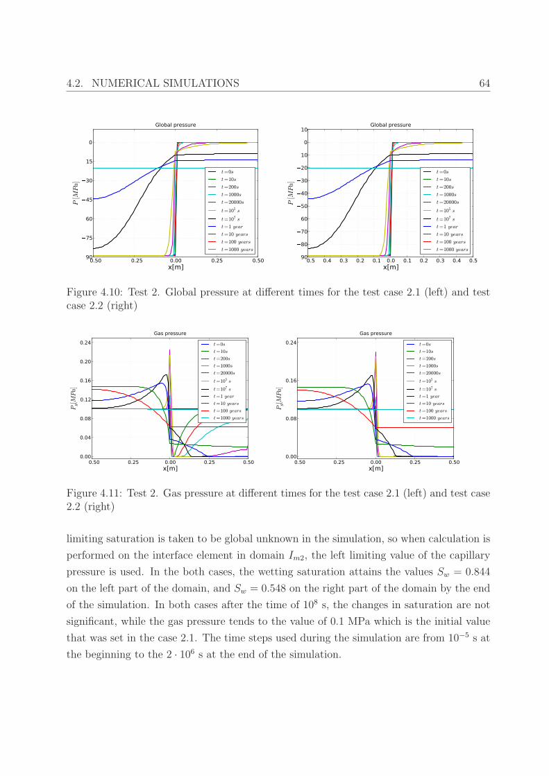
4.2. NUMERICAL SIMULATIONS 64
0.50 0.25 0.00 0.25 0.50x[m]
90
75
60
45
30
15
0
P[M
Pa]
Global pressure
t=0s
t=10s
t=200s
t=1000s
t=20000s
t=105 s
t=107 s
t=1 year
t=10 years
t=100 years
t=1000 years 0.50.40.30.20.1 0.0 0.1 0.2 0.3 0.4 0.5x[m]
90
80
70
60
50
40
30
20
10
0
10
P[M
Pa]
Global pressure
t=0s
t=10s
t=200s
t=1000s
t=20000s
t=105 s
t=107 s
t=1 year
t=10 years
t=100 years
t=1000 years
Figure 4.10: Test 2. Global pressure at different times for the test case 2.1 (left) and testcase 2.2 (right)
0.50 0.25 0.00 0.25 0.50x[m]
0.00
0.04
0.08
0.12
0.16
0.20
0.24
Pg[MPa]
Gas pressure
t=0s
t=10s
t=200s
t=1000s
t=20000s
t=105 s
t=107 s
t=1 year
t=10 years
t=100 years
t=1000 years 0.50 0.25 0.00 0.25 0.50x[m]
0.00
0.08
0.16
0.24
Pg[MPa]
Gas pressure
t=0s
t=10s
t=200s
t=1000s
t=20000s
t=105 s
t=107 s
t=1 year
t=10 years
t=100 years
t=1000 years
Figure 4.11: Test 2. Gas pressure at different times for the test case 2.1 (left) and test case2.2 (right)
limiting saturation is taken to be global unknown in the simulation, so when calculation is
performed on the interface element in domain Im2, the left limiting value of the capillary
pressure is used. In the both cases, the wetting saturation attains the values Sw = 0.844
on the left part of the domain, and Sw = 0.548 on the right part of the domain by the end
of the simulation. In both cases after the time of 108 s, the changes in saturation are not
significant, while the gas pressure tends to the value of 0.1 MPa which is the initial value
that was set in the case 2.1. The time steps used during the simulation are from 10−5 s at
the beginning to the 2 · 106 s at the end of the simulation.
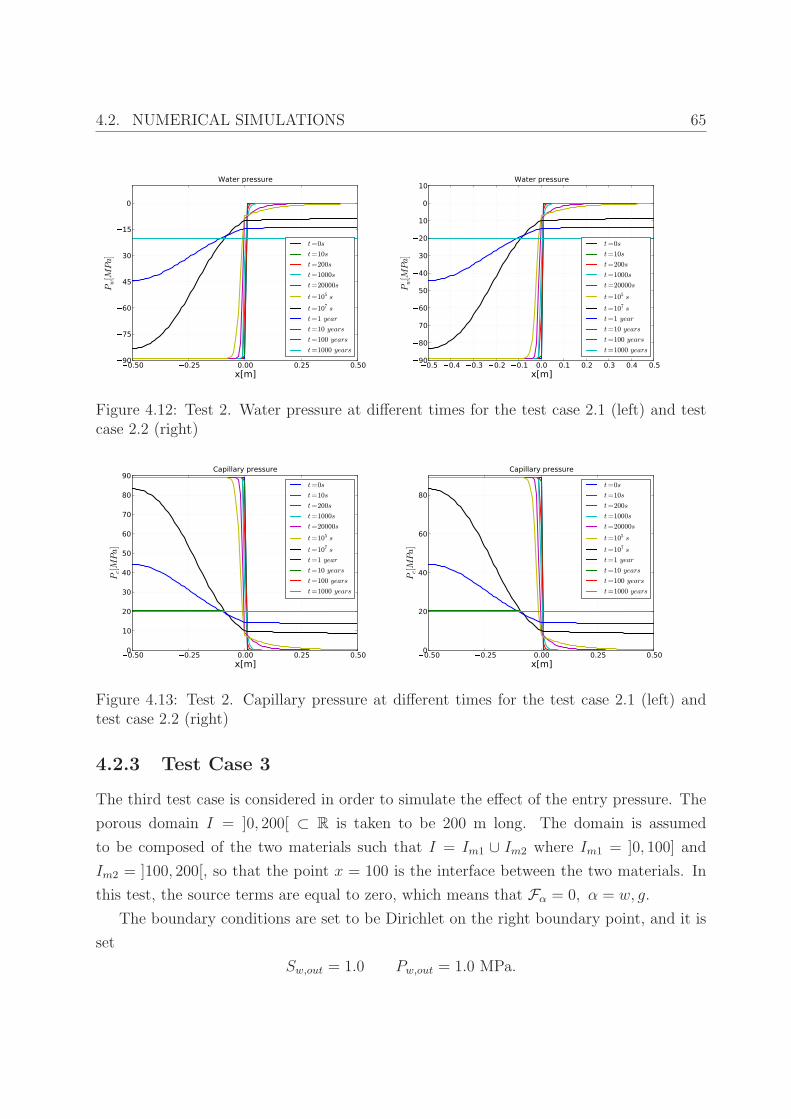
4.2. NUMERICAL SIMULATIONS 65
0.50 0.25 0.00 0.25 0.50x[m]
90
75
60
45
30
15
0
Pw[M
Pa]
Water pressure
t=0s
t=10s
t=200s
t=1000s
t=20000s
t=105 s
t=107 s
t=1 year
t=10 years
t=100 years
t=1000 years 0.50.40.30.20.1 0.0 0.1 0.2 0.3 0.4 0.5x[m]
90
80
70
60
50
40
30
20
10
0
10
Pw[M
Pa]
Water pressure
t=0s
t=10s
t=200s
t=1000s
t=20000s
t=105 s
t=107 s
t=1 year
t=10 years
t=100 years
t=1000 years
Figure 4.12: Test 2. Water pressure at different times for the test case 2.1 (left) and testcase 2.2 (right)
0.50 0.25 0.00 0.25 0.50x[m]
0
10
20
30
40
50
60
70
80
90
Pc[MPa]
Capillary pressure
t=0s
t=10s
t=200s
t=1000s
t=20000s
t=105 s
t=107 s
t=1 year
t=10 years
t=100 years
t=1000 years 0.50 0.25 0.00 0.25 0.50x[m]
0
20
40
60
80
Pc[MPa]
Capillary pressure
t=0s
t=10s
t=200s
t=1000s
t=20000s
t=105 s
t=107 s
t=1 year
t=10 years
t=100 years
t=1000 years
Figure 4.13: Test 2. Capillary pressure at different times for the test case 2.1 (left) andtest case 2.2 (right)
4.2.3 Test Case 3
The third test case is considered in order to simulate the effect of the entry pressure. The
porous domain I = ]0, 200[ ⊂ R is taken to be 200 m long. The domain is assumed
to be composed of the two materials such that I = Im1 ∪ Im2 where Im1 = ]0, 100] and
Im2 = ]100, 200[, so that the point x = 100 is the interface between the two materials. In
this test, the source terms are equal to zero, which means that Fα = 0, α = w, g.
The boundary conditions are set to be Dirichlet on the right boundary point, and it is
set
Sw,out = 1.0 Pw,out = 1.0 MPa.
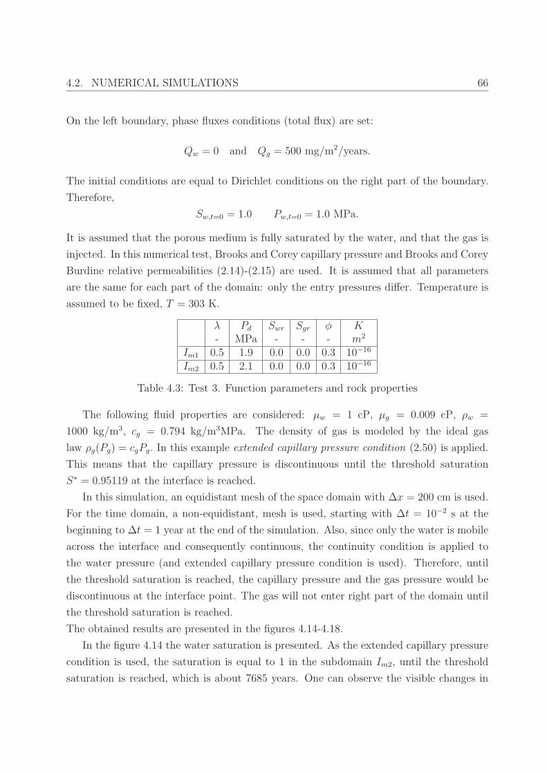
4.2. NUMERICAL SIMULATIONS 66
On the left boundary, phase fluxes conditions (total flux) are set:
Qw = 0 and Qg = 500 mg/m2/years.
The initial conditions are equal to Dirichlet conditions on the right part of the boundary.
Therefore,
Sw,t=0 = 1.0 Pw,t=0 = 1.0 MPa.
It is assumed that the porous medium is fully saturated by the water, and that the gas is
injected. In this numerical test, Brooks and Corey capillary pressure and Brooks and Corey
Burdine relative permeabilities (2.14)-(2.15) are used. It is assumed that all parameters
are the same for each part of the domain: only the entry pressures differ. Temperature is
assumed to be fixed, T = 303 K.
λ Pd Swr Sgr φ K- MPa - - - m2
Im1 0.5 1.9 0.0 0.0 0.3 10−16
Im2 0.5 2.1 0.0 0.0 0.3 10−16
Table 4.3: Test 3. Function parameters and rock properties
The following fluid properties are considered: µw = 1 cP, µg = 0.009 cP, ρw =
1000 kg/m3, cg = 0.794 kg/m3MPa. The density of gas is modeled by the ideal gas
law ρg(Pg) = cgPg. In this example extended capillary pressure condition (2.50) is applied.
This means that the capillary pressure is discontinuous until the threshold saturation
S∗ = 0.95119 at the interface is reached.
In this simulation, an equidistant mesh of the space domain with ∆x = 200 cm is used.
For the time domain, a non-equidistant, mesh is used, starting with ∆t = 10−2 s at the
beginning to ∆t = 1 year at the end of the simulation. Also, since only the water is mobile
across the interface and consequently continuous, the continuity condition is applied to
the water pressure (and extended capillary pressure condition is used). Therefore, until
the threshold saturation is reached, the capillary pressure and the gas pressure would be
discontinuous at the interface point. The gas will not enter right part of the domain until
the threshold saturation is reached.
The obtained results are presented in the figures 4.14-4.18.
In the figure 4.14 the water saturation is presented. As the extended capillary pressure
condition is used, the saturation is equal to 1 in the subdomain Im2, until the threshold
saturation is reached, which is about 7685 years. One can observe the visible changes in
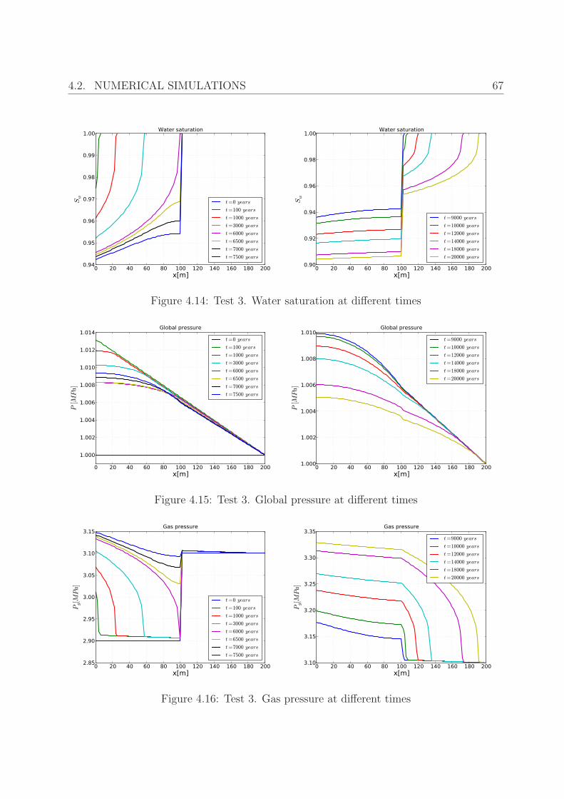
4.2. NUMERICAL SIMULATIONS 67
0 20 40 60 80 100 120 140 160 180 200x[m]
0.94
0.95
0.96
0.97
0.98
0.99
1.00
Sw
Water saturation
t=0 years
t=100 years
t=1000 years
t=3000 years
t=6000 years
t=6500 years
t=7000 years
t=7500 years
0 20 40 60 80 100 120 140 160 180 200x[m]
0.90
0.92
0.94
0.96
0.98
1.00
Sw
Water saturation
t=9000 years
t=10000 years
t=12000 years
t=14000 years
t=18000 years
t=20000 years
Figure 4.14: Test 3. Water saturation at different times
0 20 40 60 80 100 120 140 160 180 200x[m]
1.000
1.002
1.004
1.006
1.008
1.010
1.012
1.014
P[M
Pa]
Global pressure
t=0 years
t=100 years
t=1000 years
t=3000 years
t=6000 years
t=6500 years
t=7000 years
t=7500 years
0 20 40 60 80 100 120 140 160 180 200x[m]
1.000
1.002
1.004
1.006
1.008
1.010
P[M
Pa]
Global pressure
t=9000 years
t=10000 years
t=12000 years
t=14000 years
t=18000 years
t=20000 years
Figure 4.15: Test 3. Global pressure at different times
0 20 40 60 80 100 120 140 160 180 200x[m]
2.85
2.90
2.95
3.00
3.05
3.10
3.15
Pg[MPa]
Gas pressure
t=0 years
t=100 years
t=1000 years
t=3000 years
t=6000 years
t=6500 years
t=7000 years
t=7500 years
0 20 40 60 80 100 120 140 160 180 200x[m]
3.10
3.15
3.20
3.25
3.30
3.35
Pg[MPa]
Gas pressure
t=9000 years
t=10000 years
t=12000 years
t=14000 years
t=18000 years
t=20000 years
Figure 4.16: Test 3. Gas pressure at different times
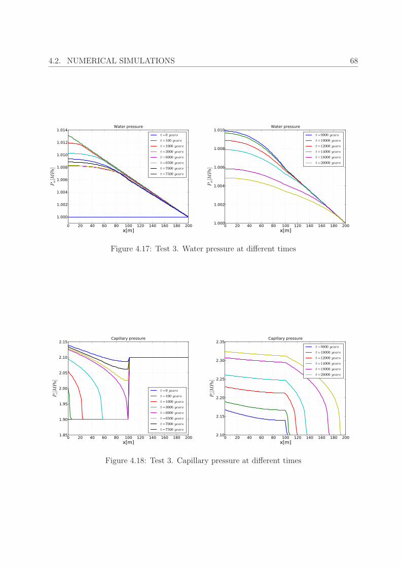
4.2. NUMERICAL SIMULATIONS 68
0 20 40 60 80 100 120 140 160 180 200x[m]
1.000
1.002
1.004
1.006
1.008
1.010
1.012
1.014
Pw[M
Pa]
Water pressure
t=0 years
t=100 years
t=1000 years
t=3000 years
t=6000 years
t=6500 years
t=7000 years
t=7500 years
0 20 40 60 80 100 120 140 160 180 200x[m]
1.000
1.002
1.004
1.006
1.008
1.010
Pw[M
Pa]
Water pressure
t=9000 years
t=10000 years
t=12000 years
t=14000 years
t=18000 years
t=20000 years
Figure 4.17: Test 3. Water pressure at different times
0 20 40 60 80 100 120 140 160 180 200x[m]
1.85
1.90
1.95
2.00
2.05
2.10
2.15
Pc[MPa]
Capillary pressure
t=0 years
t=100 years
t=1000 years
t=3000 years
t=6000 years
t=6500 years
t=7000 years
t=7500 years
0 20 40 60 80 100 120 140 160 180 200x[m]
2.10
2.15
2.20
2.25
2.30
2.35
Pc[MPa]
Capillary pressure
t=9000 years
t=10000 years
t=12000 years
t=14000 years
t=18000 years
t=20000 years
Figure 4.18: Test 3. Capillary pressure at different times
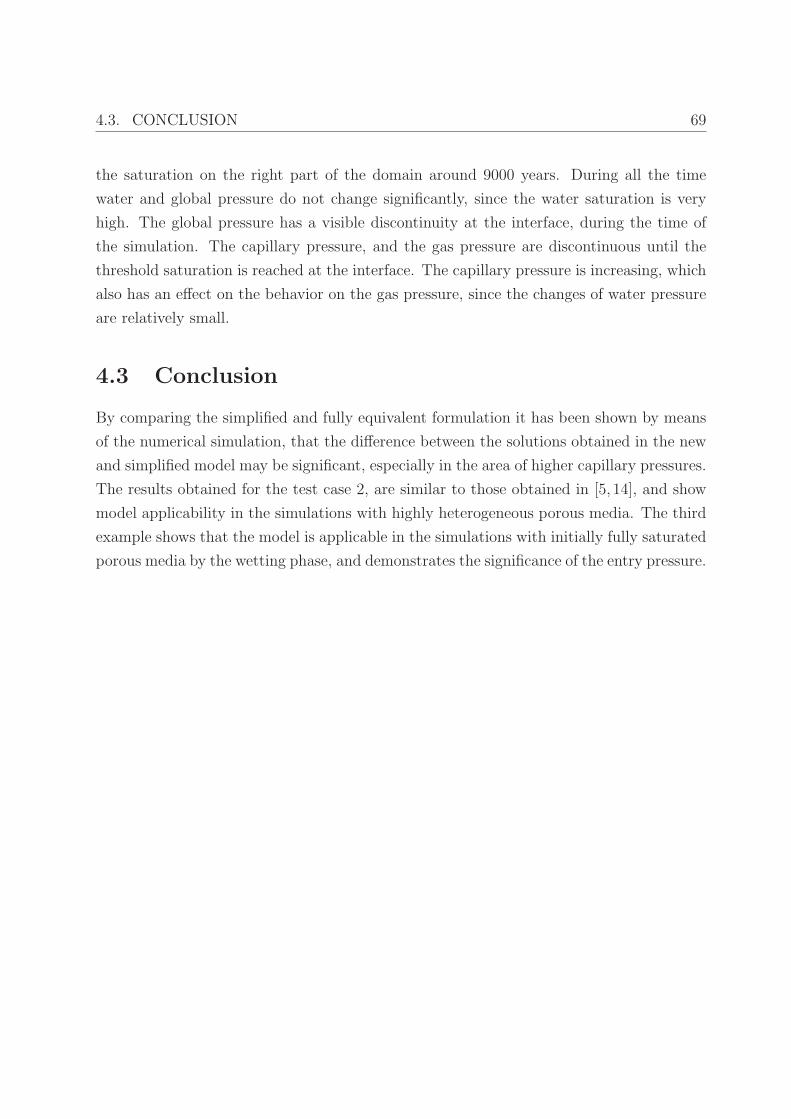
4.3. CONCLUSION 69
the saturation on the right part of the domain around 9000 years. During all the time
water and global pressure do not change significantly, since the water saturation is very
high. The global pressure has a visible discontinuity at the interface, during the time of
the simulation. The capillary pressure, and the gas pressure are discontinuous until the
threshold saturation is reached at the interface. The capillary pressure is increasing, which
also has an effect on the behavior on the gas pressure, since the changes of water pressure
are relatively small.
4.3 Conclusion
By comparing the simplified and fully equivalent formulation it has been shown by means
of the numerical simulation, that the difference between the solutions obtained in the new
and simplified model may be significant, especially in the area of higher capillary pressures.
The results obtained for the test case 2, are similar to those obtained in [5, 14], and show
model applicability in the simulations with highly heterogeneous porous media. The third
example shows that the model is applicable in the simulations with initially fully saturated
porous media by the wetting phase, and demonstrates the significance of the entry pressure.
70
Chapter 5
Existence Theory for the Two-phase
Immiscible, Compressible Flow
Model in Global Pressure
Formulation
The aim of this chapter is to establish existence of weak solutions for a new formulation for
immiscible, compressible, two-phase flows under realistic assumptions. The main difficul-
ties related to the mathematical analysis of such equations are the coupling, the degeneracy
of the diffusion term in the saturation equation and the degeneracy of the temporal term
in the global pressure equation. In the following section a short description of the math-
ematical and physical model used in this study is given. Afterwards the assumptions on
data are formulated. The existence is shown with the help of a regularized system, a time
discretization, a priori estimates and compactness arguments. This chapter contains re-
sults from [9] In section 5.2 the regularized problem is defined with a parameter η > 0,
some auxiliary results are established and the existence of weak solutions of the problem
in the non-degenerate case which will be proved in section 5.3 is formulated. The proof
will be done in three main steps. In subsection 5.3.1, a small parameter h > 0 is used
and approximate solutions are constructed with a time discretization. The existence of the
weak solutions for the corresponding system and a maximum principle for the saturation
is proved. In subsection 5.3.2, suitable test functions introduced in [44] are used to get
uniform estimates with respect to h. These estimates permit passing to the limit when
h tends to zero and obtaining the existence of weak solutions for the regularized problem
5.1. MAIN RESULTS 71
which is carried out in subsection 5.3.3. Section 5.5 is devoted to the presentation of the
result for the degenerate case.
5.1 Main Results
Recall that the mass balance equations and the Darcy law for each phase α ∈ w, g can
be written as
Φ∂
∂t(ρα(Pα)Sα) + div(ρα(Pα)qα) = Fα, qα = −λα(Sα)K(∇Pα − ρα(Pα)g), (5.1)
where Φ and K are the porosity and the absolute permeability of the porous medium, and
g is the gravitational, downward-pointing, constant vector. The source terms Fα will be
precised in the sequel.
Here, the governing equations are rewritten firstly by choosing the nonwetting satura-
tion Sg and the global pressure P as primary unknowns. All the coefficients are considered
to be functions of Sg and P , as written in remark 3.2. The superscript n used in the
same remark 3.2 is omitted for the simplicity of the notation from now on. The following
functions are introduced:
Λα(Sg, P ) = λα(Sα)ρα(Sg, P )ω(Sg, P ), α = w, g.
From the definitions of nonwetting, and wetting pressure (3.27) and (3.28), it follows that
the mass fluxes can be rewritten as
ρw(Pw)qw = −Λw(Sg, P )K∇P + a(Sg, P )K∇Sg + λw(Sg)ρw(Sg, P )2Kg,
ρg(Pg)qg = −Λg(Sg, P )K∇P − a(Sg, P )K∇Sg + λg(Sg)ρg(Sg, P )2Kg,
and consequently the differential equations of the two-phase, compressible, immiscible flow
(5.1) can now be written as (cf. [7, 8]):
Φ∂
∂t(ρw(Sg, P )Sw) − div(Λw(Sg, P )K∇P ) + div(a(Sg, P )K∇Sg)
+ div(λw(Sg)ρw(Sg, P )2Kg) + ρw(Sg, P )fw(Sg, P )FP = ρw(Sg, P )S∗
wFI ,(5.2)
5.1. MAIN RESULTS 72
Φ∂
∂t(ρg(Sg, P )Sg) − div(Λg(Sg, P )K∇P ) − div(a(Sg, P )K∇Sg)
+ div(λg(Sg)ρg(Sg, P )2Kg) + ρg(Sg, P )fg(Sg, P )FP = ρg(Sg, P )S∗
gFI ,(5.3)
where Sw = 1 − Sg, FI , FP ≥ 0 are given injection and production rates and S∗
α is known
saturation determining the composition of the injected fluid. Note that the choice of S = Sg
as primary saturation variable is motivated by the fact that Sg 7→ Pc(Sg) is an increasing
function. A priori estimates that will be used in the sequel are based on the integrability
of the quadratic terms λα(Sg)K∇Pα · ∇Pα. In presence of unbounded capillary pressure
function Pc, the non-wetting phase saturation Sg will be replaced by a new variable θ (as
in [6]),
θ = β(S) =
∫ S
0
√
λg(s)λw(s)P ′
c(s) ds, (5.4)
which is well defined since β is strictly increasing. Finally, introducing the function
A(Sg, P ) = ρw(Sg, P )ρg(Sg, P )
√
λw(Sw)λg(Sg)
λ(Sg, P )(5.5)
the system (5.2), (5.3) can be rewritten as
Φ∂
∂t(ρw(Sg, P )Sw) − div(Λw(Sg, P )K∇P ) + div(A(Sg, P )K∇θ)
+ div(λw(Sg)ρw(Sg, P )2Kg) + ρw(Sg, P )fw(Sg, P )FP = ρw(Sg, P )S∗
wFI ,(5.6)
Φ∂
∂t(ρg(Sg, P )Sg) − div(Λg(Sg, P )K∇P ) − div(A(Sg, P )K∇θ)
+ div(λg(Sg)ρg(Sg, P )2Kg) + ρg(Sg, P )fg(Sg, P )FP = ρg(Sg, P )S∗
gFI ,(5.7)
where Sg = S(θ) and Sw = 1 − Sg and the phase mass fluxes are:
Qw = ρw(Pw)qw = −Λw(Sg, P )K∇P + A(Sg, P )K∇θ + λw(Sg)ρw(Sg, P )2Kg,
Qg = ρg(Pg)qg = −Λg(Sg, P )K∇P − A(Sg, P )K∇θ + λg(Sg)ρg(Sg, P )2Kg.
Boundary conditions: let Ω ⊂ Rd, d = 2, 3, be a bounded, Lipschitz domain with
its boundary divided in two parts, ∂Ω = Γinj ∪ Γimp, where Γinj denotes the injection
boundary, and Γimp denotes the impervious one. Let ]0, T [ be the time interval of interest
5.1. MAIN RESULTS 73
and QT = Ω×]0, T [. Setting
θ = 0, P = 0 on Γinj×]0, T [ (5.8)
qw · n = qg · n = 0 on Γimp×]0, T [, (5.9)
where n is the outward pointing unit normal on ∂Ω and qα being the volumetric velocity
of the α-phase, α = w, g.
Initial conditions are given by
θ(x, 0) = θ0(x), P (x, 0) = p0(x) in Ω. (5.10)
The assumptions needed to prove an existence result for the coupled system (5.6), (5.7)
with boundary and initial conditions (5.8), (5.9) and (5.10) are:
(A.1) The porosity Φ belongs to L∞(Ω), and there exist constants, φM ≥ φm > 0, such
that 0 < φm ≤ Φ(x) ≤ φM a.e. in Ω.
(A.2) The permeability tensor K belongs to (L∞(Ω))d×d, and there exist constants kM ≥km > 0, such that for almost all x ∈ Ω and all ξ ∈ R
d it holds:
km|ξ|2 ≤ K(x)ξ · ξ ≤ kM |ξ|2.
(A.3) Relative mobilities satisfy λw, λg ∈ C([0, 1]; R+), λw(Sw = 0) = 0 and λg(Sg = 0) = 0;
λj is a non decreasing function of Sj. Moreover, there exist constants λM ≥ λm > 0
such that for all Sg ∈ [0, 1]
0 < λm ≤ λw(Sg) + λg(Sg) ≤ λM .
(A.4) There exist constants pc,min > 0 and M > 0 such that the capillary pressure function
Sg 7→ Pc(Sg), Pc ∈ C([0, 1[; R+) ∩ C1(]0, 1[; R+), for all Sg ∈]0, 1[ satisfy
P ′
c(Sg) ≥ pc,min > 0, (5.11)
Pc(Sg)(1 − Sg) +
∫ 1
0
Pc(s) ds+√
λg(Sg)λw(Sg)P′
c(Sg) ≤M. (5.12)
5.1. MAIN RESULTS 74
(A.5) There exist S# ∈]0, 1[, 0 < γ and M > 0 such that for all S ∈]0, S#]
S−γλg(S)(Pc(S) − Pc(0)) + S2−γP ′
c(S) ≤M, (5.13)
and for all S ∈ [S#, 1[
(1 − S)2−γP ′
c(S) ≤M. (5.14)
(A.6) ρw and ρg are C1(R) non decreasing functions, and there exist ρm, ρM > 0 such that
for all p ∈ R it holds
ρm ≤ ρw(p), ρg(p) ≤ ρM , 0 < ρ′w(p), ρ′g(p) ≤ ρM .
(A.7) FI , FP ∈ L2(QT ), FI , FP ≥ 0, and 0 ≤ S∗
w ≤ 1 a.e. in QT .
(A.8) There exist 0 < τ < 1 and C > 0 such that for all S1, S2 ∈ [0, 1]
C
∣
∣
∣
∣
∫ S2
S1
√
λg(s)λw(s) ds
∣
∣
∣
∣
τ
≥ |S1 − S2|.
(A.9) S∗
g = 1.
The assumptions (A.1)–(A.3) and (A.7)–(A.8) are classical for two-phase flow in porous
media. The assumptions (A.4) and (A.5) control the strength of singularities in the capillary
pressure and its derivative at the end points S = 0, 1, and it will be commented further
on. The assumption (A.6) is satisfied by mass densities given by a physical law, such as
the ideal gas law, by correcting the density function for extremely small and large pressure
values. Such correction does not influence the system behavior in physically admissible
range of pressures, and therefore (A6) does not limit the applicability of our result.
Remark 5.1. Under assumptions (A.3), (A.4) and (A.6), it is easy to see that (3.27) has
a unique solution Pg ∈ C([0, 1] × R) ∩ C1(]0, 1] × R) and consequently Pw ∈ C1([0, 1[×R).
Using the boundedness of Pc(Sg)(1 − Sg) in (A.4), it is easy to see that there exists a
constant M such that for all Sg ∈ [0, 1],
P ≤ Pg(Sg, P ) ≤ P +M, P (1 − Sg) −M ≤ Pw(Sg, P )(1 − Sg) ≤ P (1 − Sg).
5.1. MAIN RESULTS 75
The wetting phase pressure Pw, in contrast to Pg, is unbounded when Sg → 1. From (A.3)
and (A.6) it also follows that ω is smooth, strictly positive and bounded function. There
exist constants ωm, ωM , such that for all Sg ∈ [0, 1] and P ∈ R,
0 < ωm ≤ ω(Sg, P ) ≤ ωM < +∞,
and also
0 < ρmλmωm ≤ Λ(Sg, P ) = Λw(Sg, P ) + Λg(Sg, P ) ≤ ρMλMωM .
Remark 5.2. From (A.5) it follows that there exists a constant C > 0 such that for all
S1, S2 ∈]0, S#]
|Pc(S1) − Pc(S2)|min(S1, S2) ≤ C|S1 − S2|γ, (5.15)
and for all S1, S2 ∈ [S#, 1[
|Pc(S1) − Pc(S2)|(1 − max(S1, S2)) ≤ C|S1 − S2|γ. (5.16)
For example, for S1 < S2 < S#
|Pc(S1) − Pc(S2)|min(S1, S2) = S1(Pc(S2) − Pc(S1)) ≤∫ S2
S1
sP ′
c(s) ds
=
∫ S2
S1
s2−γP ′
c(s)sγ−1 ds ≤ C
∫ S2
S1
sγ−1 ds ≤ C
γ|S1 − S2|γ,
and analogously for S1 > S2. The estimate (5.16) can be proved in a similar way. For
S# < S1 < S2
|Pc(S1) − Pc(S2)|(1 − max(S1, S2)) = (1 − S2)(Pc(S2) − Pc(S1)) ≤∫ S2
S1
(1 − s)P ′
c(s) ds
=
∫ S2
S1
(1 − s)2−γP ′
c(s)(1 − s)γ−1 ds ≤ C
∫ S2
S1
(1 − s)γ−1
=C
γ((1 − S1)
γ − (1 − S2)γ) ≤ C
γ|S1 − S2|γ
where the last inequality follows from the fact that the function (1−S)γ is Holder continuous
with exponent γ, when 0 < γ ≤ 1. The case S1 > S2 can be shown analogously.
5.1. MAIN RESULTS 76
Remark 5.3. Note that (A.8) is satisfied if the function α(S) =√
λg(S)λw(S) has the
following asymptotic behavior at S = 0, 1:
α(S) ≥ C0
Sγ1 for S ≤ S0
(1 − S)γ2 for S ≥ S0
Then (A.8) is fulfilled for τ = min(1/(1 + γ1), 1/(1 + γ2)). Furthermore, (A.4) and (A.8)
imply that S 7→ β(S) is a monotone increasing function satisfying β(1) < +∞ and thus
there exists an inverse function S = β−1 : [0, β(1)] → [0, 1]. From (A.8) it follows
|β(S2) − β(S1)|τ ≥pτ
c,min
C|S2 − S1|, (5.17)
and S is Holder continuous with exponent τ .
Remark 5.4. Conditions (A.4) and (A.5) are satisfied for many relative permeability-
capillary pressure models in suitable range of theirs parameters. A calculation can show,
that Brooks and Corey model satisfy (A.4) and (A.5) for parameter λ > 1 and any γ ≤ 1− 1λ.
For van Genuchten’s functions these conditions are satisfied for n > 2 and any γ ≤ n−2n−1
.
In order to take into account the Dirichlet boundary condition the following space is in-
troduced:
V = ϕ ∈ H1(Ω) : ϕ|Γinj= 0.
Throughout the rest of the chapter the notation S = Sg is used. Now the existence result
of weak solutions of the system (5.6), (5.7), (5.8), (5.9) and (5.10) in variables P and θ is
presented.
Theorem 5.1. Let (A.1)-(A.8) hold and assume (θ0, p0) ∈ L2(Ω) × L2(Ω), 0 ≤ θ0 ≤ β(1)
a.e. in Ω. Then there exists (P, θ) satisfying
P ∈ L2(0, T ;V ), θ ∈ L2(0, T ;V ), 0 ≤ θ ≤ β(1) a.e. in QT , S = S(θ),
Φ∂t(ρw(S, P )(1 − S)) ∈ L2(0, T ;V ′), Φ∂t(ρg(S, P )S) ∈ L2(0, T ;V ′),
5.1. MAIN RESULTS 77
for all ϕ, ψ ∈ L2(0, T ;V )
∫ T
0
〈Φ∂t(ρw(S, P )(1 − S)), ϕ〉dt+
∫
QT
[Λw(S, P )K∇P · ∇ϕ− A(S, P )K∇θ · ∇ϕ]dxdt
−∫
QT
[λw(S)ρw(S, P )2Kg · ∇ϕ− ρw(S, P )fw(S, P )FPϕ]dxdt = 0, (5.18)
∫ T
0
〈Φ∂t(ρg(S, P )S), ψ〉dt+
∫
QT
[Λg(S, P )K∇P · ∇ψ + A(S, P )K∇θ · ∇ψ]dxdt
−∫
QT
[λg(S)ρg(S, P )2Kg · ∇ψ − ρg(S, P )fg(S, P )FPψ]dxdt (5.19)
=
∫
QT
ρg(S, P )FIψdxdt.
Furthermore, for all ψ ∈ V the functions
t 7→∫
Ω
Φρw(Pw(S, P ))(1 − S)ψdx, t 7→∫
Ω
Φρg(Pg(S, P ))Sψdx
are continuous in [0, T ] and the initial condition is satisfied in the following sense:
(∫
Ω
Φρw(Pw(S, P ))(1 − S)ψdx
)
(0) =
∫
Ω
Φρw(Pw(s0, p0))(1 − s0)ψdx,
(∫
Ω
Φρg(Pg(S, P ))Sψdx
)
(0) =
∫
Ω
Φρg(Pg(s0, p0))s0ψdx,
where s0 = S(θ0).
Compared to [44, 48], this existence result permits to consider unbounded capillary
pressure functions and can be applied to physically relevant situations. In contrast to
[42–44] and [48], no additional regularity of porosity and permeability fields apart from
boundedness and positivity are demanded. This is achieved by a modification of a standard
compactness result in [60]. By considering this new model for immiscible compressible two-
phase flow in porous media by the concept of global pressure, the proof of the existence of
weak solutions greatly simplifies compared to the one presented in [42–44,48].
5.2. REGULARISED PROBLEM AND AUXILIARY RESULTS 78
5.2 Regularised Problem and Auxiliary Results
In the proof of Theorem 5.1 a crucial role is played by the fact that the change of variables
(u, v) = G(S, P ) given by
u = ρw(Pw(S, P ))(1 − S), v = ρg(Pg(S, P ))S (5.20)
(S = Sg) is a diffeomorphism. This is proved in the next two lemmas.
Lemma 5.1. Assume (A.4) and (A.6) hold. Then the map (u, v) = G(S, P ), G : [0, 1] ×R → [0, ρM ] × [0, ρM ] defined by (5.20) is injective.
Proof. Assume that there exist (S1, P1) 6= (S2, P2) such that
ρw(Pw(S1, P1))(1 − S1) = ρw(Pw(S2, P2))(1 − S2),
ρg(Pg(S1, p1))S1 = ρg(Pg(S2, P2))S2.
First the case S1 = S2 is considered. If S1 = S2(= S) > 0 then the strict monotonicity of
ρg gives Pg(S, P1) = Pg(S, P2). The nonwetting pressure Pg is strictly monotone function of
the global pressure, leading to P1 = P2. The argument is also valid in the case S = 1 since
Pg(1, P ) is finite. If S1 = S2 = 0 then ρw(Pw(0, P1)) = ρw(Pw(0, P2)) or ρw(P1) = ρw(P2)
which leads again to P1 = P2.
Consider the case S1 > S2. Then
S2
S1
< 1 and1 − S1
1 − S2
< 1.
From
ρw(Pw(S1, P1))1 − S1
1 − S2
= ρw(Pw(S2, P2)), ρg(Pg(S1, P1)) = ρg(Pg(S2, P2))S2
S1
.
it follows that
ρw(Pw(S1, P1)) > ρw(Pw(S2, P2)), ρg(Pg(S1, P1)) < ρg(Pg(S2, P2)).
The density functions are strictly increasing and therefore
Pw(S1, P1) > Pw(S2, P2), Pg(S1, P1) < Pg(S2, P2).
5.2. REGULARISED PROBLEM AND AUXILIARY RESULTS 79
By subtraction one obtains
Pc(S1) = Pg(S1, P1) − Pw(S1, P1) < Pc(S2) = Pg(S2, P2) − Pw(S2, P2)
which leads to S1 < S2 since S = Sg → Pc(S) is strictly increasing function. This is in
contradiction with starting assumption, S1 > S2. In the same way, one may prove that the
case S1 < S2 is not possible and the conclusion follows.
In order to study the map G, given by (5.20), it is decomposed as G = G2 G1,
(S, P ) 7→ (S, Pg(S, P )) 7→ (ρw(Pg − Pc(S))(1 − S), ρg(Pg)S).
Mapping G1(S, P ) = (S, Pg(S, P )) is a homeomorphism from [0, 1]×R to [0, 1]×R, and a
diffeomorphism in ]0, 1[×R.
Next, consider the mapping G2(S, Pg) = (ρw(Pg − Pc(S))(1 − S), ρg(Pg)S). A simple
analysis shows that G2 maps [0, 1]×R into lower triangle of [0, ρw,max]× [0, ρg,max]. Indeed,
if one sets
u = ρw(Pg − Pc(S))(1 − S), v = ρg(Pg)S,
then, for a fixed v ∈ [0, ρg,max], S is allowed to vary in the interval
v
ρg,max
≤ S ≤ min(1,v
ρg,min
).
u is expressed as a function of S (and v which is fixed) as
u = ρw(ρ−1g (
v
S) − Pc(S))(1 − S).
This function is strictly decreasing since
du
dS= −ρw(ρ−1
g (v
S) − Pc(S)) + ρ′w(ρ−1
g (v
S) − Pc(S))(1 − S)(Dρ−1
g (v
S)(− v
S2) − P ′
c(S)) < 0.
One easily see that (u, v) covers all of shadowed region on Figure 5.2, which will be denoted
by R. Note that R contains open segments BC and DA, but it does not contain closed
segments AB and CD which correspond, respectively, to Pg = +∞ and Pg = −∞.
Lemma 5.2. The mappings G and G2 are homeomorphisms from [0, 1] × R to R and
diffeomorphisms from ]0, 1[×R to Int(R).
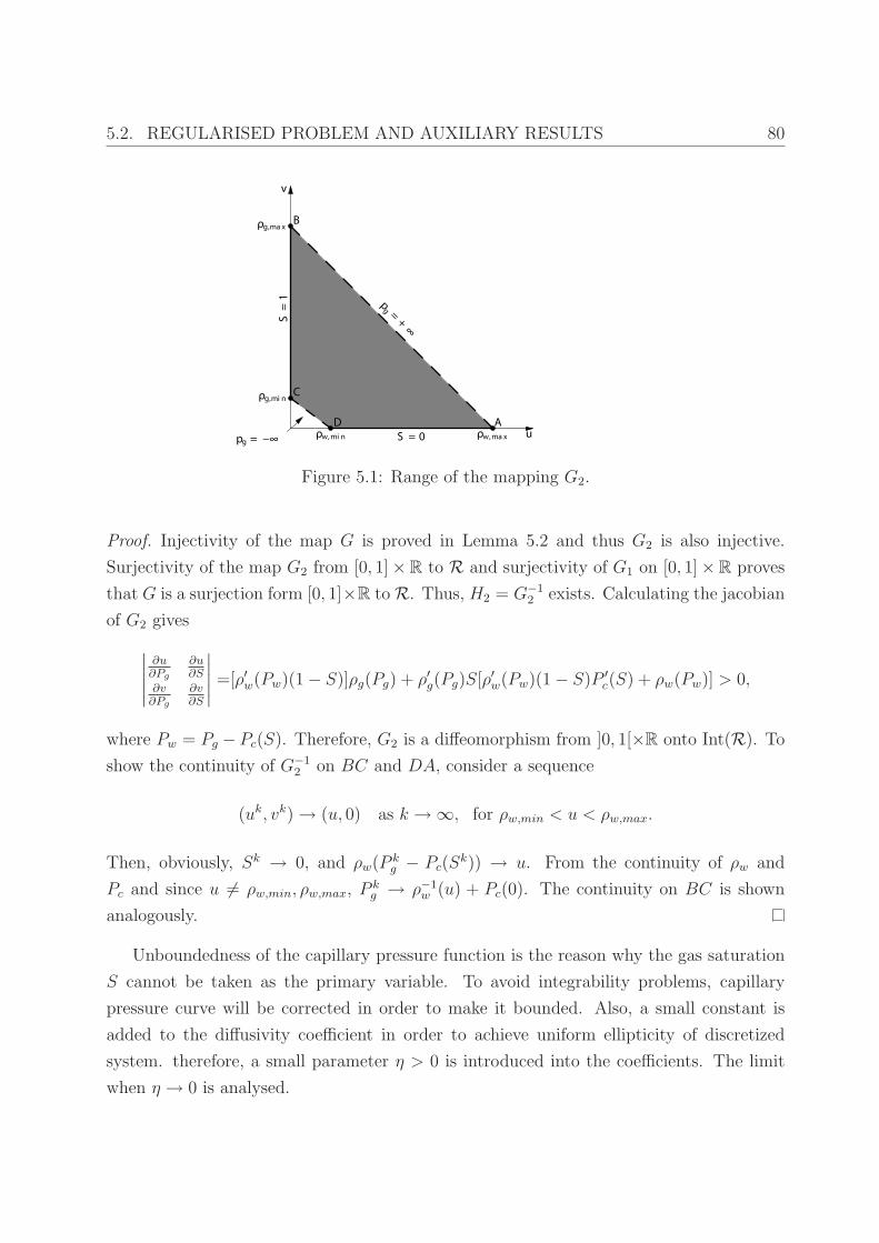
5.2. REGULARISED PROBLEM AND AUXILIARY RESULTS 80
Figure 5.1: Range of the mapping G2.
Proof. Injectivity of the map G is proved in Lemma 5.2 and thus G2 is also injective.
Surjectivity of the map G2 from [0, 1]× R to R and surjectivity of G1 on [0, 1]× R proves
that G is a surjection form [0, 1]×R to R. Thus, H2 = G−12 exists. Calculating the jacobian
of G2 gives
∣
∣
∣
∣
∣
∂u∂Pg
∂u∂S
∂v∂Pg
∂v∂S
∣
∣
∣
∣
∣
=[ρ′w(Pw)(1 − S)]ρg(Pg) + ρ′g(Pg)S[ρ′w(Pw)(1 − S)P ′
c(S) + ρw(Pw)] > 0,
where Pw = Pg − Pc(S). Therefore, G2 is a diffeomorphism from ]0, 1[×R onto Int(R). To
show the continuity of G−12 on BC and DA, consider a sequence
(uk, vk) → (u, 0) as k → ∞, for ρw,min < u < ρw,max.
Then, obviously, Sk → 0, and ρw(P kg − Pc(S
k)) → u. From the continuity of ρw and
Pc and since u 6= ρw,min, ρw,max, Pkg → ρ−1
w (u) + Pc(0). The continuity on BC is shown
analogously.
Unboundedness of the capillary pressure function is the reason why the gas saturation
S cannot be taken as the primary variable. To avoid integrability problems, capillary
pressure curve will be corrected in order to make it bounded. Also, a small constant is
added to the diffusivity coefficient in order to achieve uniform ellipticity of discretized
system. therefore, a small parameter η > 0 is introduced into the coefficients. The limit
when η → 0 is analysed.

5.2. REGULARISED PROBLEM AND AUXILIARY RESULTS 81
The capillary pressure derivative may be unbounded at S = 0 and S = 1. The derivative
will be limited by applying an operator Rη, 0 < η < 1, to the capillary pressure derivative
in the following way:
Rη(P′
c(S)) =
2(1 − Sη)Pc(η)−Pc(0)
η+ (2S
η− 1)P ′
c(η) for S ≤ η
P ′
c(S) for η ≤ S ≤ 1 − η
P ′
c(1 − η) for 1 − η ≤ S ≤ 1,
(5.21)
and let
P ηc (S) = Pc(0) +
∫ S
0
Rη(P′
c(s)) ds. (5.22)
Obviously, if the derivative P ′
c(S) is bounded at S = 0 or S = 1, then the correction at
that end in Rη(P′
c(S)) is not needed. It is easy to see that, for any η > 0, P ηc (S) is a
bounded, monotone, C1([0, 1]) function, and that P ηc (S) = Pc(S) for S ∈ [η, 1 − η]. From
(A.4) it follows that for sufficiently small η it holds
d
dSP η
c (S) ≥ pc,min/2 > 0. (5.23)
Also, the operator Rη satisfies
|Rη(P′
c(S))| ≤ pηc,max < +∞,
for some constant pηc,max such that, generally, pη
c,max → ∞ when η → 0. Note also that one
can assume that Rη(P′
c(S)) satisfies
Rη(P′
c(S)) ≤ P ′
c(S), for S ≥ η, (5.24)
since if it does not one can modify the definition of Rη(P′
c(S)) for S > 1−η by replacing the
constant value P ′
c(1 − η) by suitable continuous curve, staying below P ′
c(S) for S > 1 − η.
Define:
P ηg (S, P ) = P + Pc(0) +
∫ S
0
fw(s, P )Rη(P′
c(s)) ds, (5.25)
P ηw(S, P ) = P −
∫ S
0
fg(s, P )Rη(P′
c(s)) ds. (5.26)
5.2. REGULARISED PROBLEM AND AUXILIARY RESULTS 82
Obviously,
P ηg (S, P ) − P η
w(S, P ) = P ηc (S). (5.27)
The derivatives of regularized phase pressures are given as
∂P ηg
∂P=∂P η
w
∂P= ωη(S, P ),
where, from Remark 5.1
ωη(S, P ) =
exp
(
−∫ S
0
(νg(s, P ) − νw(s, P ))ρw(s, P )ρg(s, P )λw(s)λg(s)Rη(P
′
c(s))
(ρw(s, P )λw(s) + ρg(s, P )λg(s))2ds
)
.
Now it follows that
∇P ηg = ωη(S, P )∇P + fw(S, P )Rη(P
′
c(S))∇S, (5.28)
∇P ηw = ωη(S, P )∇P − fg(S, P )Rη(P
′
c(S))∇S, (5.29)
and for given P, S ∈ L2(0, T ;H1(Ω)) it follows that P ηg , P
ηw ∈ L2(0, T ;H1(Ω)).
In the regularized version of the system (5.6), (5.7) the functions P ηα instead of Pα are
used in calculations of the mass densities. That means, ρα(S, P ) is replaced with
ρηα(S, P ) = ρα(P η
α(S, P )). (5.30)
The function A(S, P ) is replaced with Aη(S, P ), for η > 0, defined as
Aη(S, P ) =ρw(S, P )ρg(S, P )
λ(S, P )λw(S)λg(S)Rη(P
′
c(S)) + η. (5.31)
Obviously, Aη(S, P ) ≥ η > 0. The regularized system now takes the form
Φ∂
∂t(ρη
w(S, P )(1 − S)) − div(Ληw(S, P )K∇P ) + div(Aη(S, P )K∇S)
+ div(λw(S)ρηw(S, P )2
Kg) + ρηw(S, P )fw(S, P )FP = ρη
w(S, P )S∗
wFI ,(5.32)
5.2. REGULARISED PROBLEM AND AUXILIARY RESULTS 83
Φ∂
∂t(ρη
g(S, P )S) − div(Ληg(S, P )K∇P ) − div(Aη(S, P )K∇S)
+ div(λg(S)ρηg(S, P )2
Kg) + ρηg(S, P )fg(Sw, P )FP = ρη
g(S, P )S∗
gFI ,(5.33)
where S = Sg and for α ∈ w, g
Ληα(S, P ) = λα(S)ρα(S, P )ωη(S, P ). (5.34)
The regularized total mobility is introduced:
Λη(S, P ) = Ληw(S, P ) + Λη
g(S, P ), (5.35)
and the regularized β function:
βη(S) =
∫ S
0
√
λw(s)λg(s)Rη(P′
c(s)) ds. (5.36)
Remark 5.5. The regularized wetting phase flux (without gravity term) can be written as:
Ληw(S, P )K∇P − Aη(S, P )K∇S = λw(S)ρw(S, P )K∇P η
w − ηK∇S, (5.37)
and similarly for the regularized non wetting flux:
Ληg(S, P )K∇P + Aη(S, P )K∇S = λg(S)ρg(S, P )K∇P η
g + ηK∇S. (5.38)
Remark 5.6. A priori estimates that will be used in the proof of Theorem 5.1 are based
on the following equality,
ρg(S, P )λg(S)K∇P ηg · ∇P η
g + ρw(S, P )λw(S)K∇P ηw · ∇P η
w
= Λη(S, p)ωη(S, p)K∇P · ∇P +ρg(S, P )ρw(S, P )
λ(S, P )K∇βη(S) · ∇βη(S).
(5.39)
From (3.27) and similarly from (3.28) one obtains
∇P ηg · ∇P η
g = ωη(S, P )2∇P · ∇P + 2ωη(S, P )fw(SP )Rη(P′
c(S))∇S · ∇P+ fw(S, P )2Rη(P
′
c(S))2∇S · ∇S.
5.2. REGULARISED PROBLEM AND AUXILIARY RESULTS 84
Then by setting U = ρg(S, P )λg(S)K∇P ηg ·∇P η
g + ρw(S, P )λw(S)K∇P ηw ·∇P η
w, one obtains
U = ωη(S, P )2(ρg(S, P )λg(S) + ρw(S, P )λw(S))K∇P · ∇P+ (ρg(S, P )λg(S)fw(S, P )2Rη(P
′
c(s))2
+ ρw(S, P )λw(S)fg(S, P )2Rη(P′
c(s))2)K∇S · ∇S
+ 2ρg(S, P )λg(S)ρw(S, P )λw(S)
λ(S, P )ωη(S, P )Rη(P
′
c(S))K∇S · ∇P
− 2ρw(S, P )λw(S)ρg(S, P )λg(S)
λ(S, P )ωη(S, P )Rη(P
′
c(S))K∇S · ∇P
which gives
U = ωη(S, P )Λη(S, P )K∇P · ∇P + (ρg(S, P )λg(S)fw(S, P )2Rη(P′
c(s))2
+ ρw(S, P )λw(S)fg(S, P )2Rη(P′
c(s))2)K∇S · ∇S.
Using the following equality (ρg = ρg(S, P ), ρw = ρw(S, P ))
ρgλg(S)ρ2wλw(S)2 + ρwλw(S)ρg)
2λg(S)2
λ(S, P )2=ρgλg(S)ρwλw(S)
λ(S, P ),
it can be obtained
U = ωη(S, P )Λη(S, P )K∇P · ∇P
+ρg(S, P )ρw(S, P )
λ(S, P )
(
√
λg(S)λw(S)Rη(P′
c(S))
)2
K∇S · ∇S,
which gives
U = ωη(S, P )Λη(S, P )K∇P · ∇P +ρg(S, P )ρw(S, P )
λ(S, P )K∇βη(S) · ∇βη(S).
From the equality (5.39) the estimate follows
ρg(S, P )λg(S)K∇P ηg · ∇P η
g + ρw(S, P )λw(S)K∇P ηw · ∇P η
w
≥ λmρmω2mkm|∇P |2 +
ρ2m
λMρM
km|∇βη(S)|2.(5.40)
Remark 5.7. From (5.23), as in Remark 5.3, that βη has Holder continuous inverse
5.2. REGULARISED PROBLEM AND AUXILIARY RESULTS 85
Sη = (βη)−1, with the same exponent τ . Indeed,
|βη(S1) − βη(S2)|τ = |∫ S2
S1
√
λw(s)λg(s)Rη(P′
c(s)) ds|τ ≥ Pc,min|∫ S2
S1
√
λw(s)λg(s) ds|τ
≥ C|S1 − S2|.
Remark 5.8. Lemma 5.2 is equally applicable to the mapping (u, v) = Gη(S, P ), Gη : [0, 1]×R → R defined by
u = ρw(P ηw(S, P ))(1 − S), v = ρg(P
ηg (S, P ))S, (5.41)
which is therefore homeomorphism from [0, 1] × R onto R.
Now the convergence properties of the regularized coefficients will be investigated when
η → 0.
Lemma 5.3. Assume that (A.4)-(A.6) are fulfilled. Then there exist constants M > 0, ωm
and ωM such that
P ≤P ηg (S, P ) ≤ P +M, (5.42)
(1 − S)P −M ≤(1 − S)P ηw(S, P ) ≤ (1 − S)P, (5.43)
λw(S)P −M ≤λw(S)P ηw(S, P ) ≤ λw(S)P, (5.44)
0 < ωm ≤ωη(S, P ) ≤ ωM , (5.45)
and the following uniform convergences in [0, 1] × R hold:
P ηg (S, P ) → Pg(S, P ) as η → 0, (5.46)
(1 − S)P ηw(S, P ) → (1 − S)Pw(S, P ) as η → 0, (5.47)
λw(S)P ηw(S, P ) → λw(S)Pw(S, P ) as η → 0, (5.48)
ωη(S, P ) → ω(S, P ) as η → 0, (5.49)
βη(S) → β(S) as η → 0 uniformly in [0, 1]. (5.50)
Proof. The estimates (5.42) and (5.43) follow easily as in Remark 5.1, by using (A.4) which
gives the boundedness of λw(S)P ′
c(S) in [S#, 1[ and the boundedness of (1 − S)Pc(S) in
[0, 1]. Similarly (5.44), and (5.45) are obtained as in Remark 5.1. For the convergence
5.2. REGULARISED PROBLEM AND AUXILIARY RESULTS 86
(5.46), using (A.4) which implies that λw(S)P ′
c(S) is bounded in vicinity of S = 1, the
estimate is:
|P ηg (S, P ) − Pg(S, P )| ≤
∫ S
0
fw(s, p)|Rη(P′
c(s)) − P ′
c(s)| ds
≤ ρM
λmρm
(
λM
∫ η
0
(Rη(P′
c(s)) + P ′
c(s)) ds+
∫ 1
1−η
λw(s)(P ′
c(1 − η) + P ′
c(s)) ds
)
≤ ρM
λmρm
(
λM
∫ η
0
(Rη(P′
c(s)) ds+ λM
∫ η
0
P ′
c(s) ds+
∫ 1
1−η
λw(1 − η)P ′
c(1 − η) ds+
+
∫ 1
1−η
λw(s)P ′
c(s) ds
)
≤ ρM
λmρm
(2λM(Pc(η) − Pc(0)) + Cη).
This gives (5.46), and (5.50) is obtained in a similar way.
|βη(S) − β(S)| ≤∫ S
0
√
λw(s)λg(s)|Rη(P′
c(s)) − p′c(s)| ds
≤∫ η
0
√
λw(S)λg(S)Rη(P′
c(s)) ds+
∫ 1
1−η
√
λw(s)λg(s)P′
c(s) ds
≤ λM
∫ η
0
Rη(P′
c(s)) ds+ Cη
= λm(Pc(η) − Pc(0)) + Cη.
For (5.47), for sufficiently small η it follows:
|(P ηw(S, P ) − Pw(S, P ))(1 − S)| ≤ ρM
λmρm
|1 − S|∫ S
0
λg(s)|Rη(P′
c(s)) − P ′
c(s)| ds
≤ ρMλM
λmρm
(
∫ η
0
(Rη(P′
c(s)) + P ′
c(s)) ds+ |1 − S|∫ max(1−η,S)
1−η
P ′
c(s) ds)
≤ ρMλM
λmρm
(2(Pc(η) − Pc(0)) + (1 − S) [Pc(max(1 − η, S)) − Pc(1 − η)]).
Applying (5.16) in Remark 5.2 one gets
|(P ηw(S, P ) − Pw(S, P ))(1 − S)| ≤ C(Pc(η) − Pc(0) + ηγ)
which gives (5.47).
The convergence (5.48) is obtained in a similar way as in (5.46) and (5.47) by using the
monotonicity of λw(S) and the fact that, due to (A.4), λw(S)P ′
c(S) is bounded in [S#, 1[.
5.2. REGULARISED PROBLEM AND AUXILIARY RESULTS 87
Therefore,
|(P ηw(S, P ) − Pw(S, P ))λw(S)| ≤ ρM
λmρm
λw(S)
∫ S
0
λg(s)|Rη(P′
c(s)) − P ′
c(s)| ds
≤ ρM
λmρm
(
∫ η
0
λw(s)λg(s) (Rη(P′
c(s)) + P ′
c(s)) ds+
∫ 1
1−η
2λw(s)λg(s)P′
c(s) ds)
≤ ρMλ2M
λmρm
(2(Pc(η) − Pc(0)) + Cη).
The convergence (5.49) is obtained similarly, using the fact that the exponential function
is continuously differentiable.
Corollary 5.1. Assume that Sη, P η, S, P ∈ L2(ΩT ) are such that 0 ≤ Sη, S ≤ 1 and
P η → P, Sη → S a.e. in QT when η → 0.
Then
P ηg (Sη, P η) → Pg(S, P ) ωη(Sη, P η) → ω(S, P ), a.e. in QT when η → 0, (5.51)
(1 − Sη)ρw(P ηw(Sη, P η)) → (1 − S)ρw(Pw(S, P )), a.e. in QT when η → 0, (5.52)
λw(Sη)ρw(P ηw(Sη, P η)) → λw(S)ρw(Pw(S, P )), a.e. in QT when η → 0. (5.53)
Proof. This is a consequence of the uniform convergence in Lemma 5.3 and the continuity
of functions Pα, ω and ρα.
The weak formulation of the regularized problem is defined in the following theorem.
Theorem 5.2. (Regularized problem) Let (A.1)-(A.7) hold and assume that (s0, p0) ∈V × V , 0 ≤ s0 ≤ 1 a.e. in Ω. For all η > 0 sufficiently small there exists (P η, Sη)
satisfying
P η, Sη ∈ L2(0, T ;V ), 0 ≤ Sη ≤ 1 a.e. in QT ,
Φ∂t(ρηw(Sη, P η)(1 − Sη)),Φ∂t(ρ
ηg(S
η, P η)Sη) ∈ L2(0, T ;V ′),
ρηw(Sη, P η)(1 − Sη), ρη
g(Sη, P η)Sη ∈ L2(0, T ;V ) ∩ C([0, T ];L2(Ω)),
5.3. PROOF OF THEOREM 5.2 88
and for all ϕ, ψ ∈ L2(0, T ;V )
∫ T
0
〈Φ∂t(ρηw(Sη, P η)(1 − Sη)), ϕ〉dt
+
∫
QT
[Ληw(Sη, P η)K∇P η · ∇ϕ− Aη(Sη, P η)K∇Sη · ∇ϕ]dxdt
−∫
QT
[λw(Sη)ρηw(Sη, P η)2
Kg · ∇ϕ− ρηw(Sη, P η)fw(Sη, P η)FPϕ]dxdt (5.54)
=
∫
QT
ρηw(Sη, P η)(1 − S∗)FIϕdxdt,
∫ T
0
〈Φ∂t(ρηg(S
η, P η)Sη), ψ〉dt
+
∫
QT
[Ληg(S
η, P η)K∇P η · ∇ψ + Aη(Sη, P η)K∇Sη · ∇ψ]dxdt
−∫
QT
[λg(Sη)ρη
g(Sη, P η)2
Kg · ∇ψ − ρηg(S
η, P η)fg(Sη, P η)FPψ]dxdt (5.55)
=
∫
QT
ρηg(S
η, P η)S∗FIψdxdt.
Furthermore, ρηw(Sη, P η)(1 − Sη) = ρη
w(s0, p0)(1 − s0) and ρηg(S
η, P η)Sη = ρηg(s0, p0)s0 a.e.
in Ω, for t = 0.
The regularization of the capillary pressure (5.21) is not needed for problem (5.54),
(5.55). The fact that the regularized function Aη is strictly positive (see (5.31)) and (A.4)
are sufficient to obtain a regularized problem, i.e. a non-degenerate one. The need for
regularization comes from the choice of the test function used in Section 5.3.2. Namely,
Pw(S, P ) is not a good test function with P, S ∈ L2(0, T ;V ) since ∇Pw(S, P ) is not in
L2(QT ) due to the singularity of ∂Pw(S, P )/∂S at S = 1. This singularity is removed by
correcting the capillary pressure curve.
5.3 Proof of Theorem 5.2
5.3.1 Step 1. Time Discretization
In this section a discretization of the time derivative for the regularized system (5.54)–
(5.55) is introduced. In order to simplify the notation, the dependence of the saturation
5.3. PROOF OF THEOREM 5.2 89
and the global pressure on the small parameter η will be omitted until the passage to the
limit η → 0.
The time derivatives in the variational formulation given in Theorem 5.2 are discretized
in the following way: For each positive integer N interval [0, T ] is divided into N subin-
tervals of equal length h = T/N . One sets tn = nh and Jn =]tn−1, tn] for 1 ≤ n ≤ N , and
denote the time difference operator by
∂hv(t) =v(t+ h) − v(t)
h,
for any h > 0. Also, for any Hilbert space H one denotes
lh(H) = v ∈ L∞(0, T ;H) : v is constant in time on each subinterval Jn ⊂ [0, T ].
For vh ∈ lh(H) is set vn = (vh)n = vh|Jnand, therefore, it can be written
vh =N∑
n=1
vnχ]tn−1,tn](t), vh(0) = v0.
To each function vh ∈ lh(H) one can assign a piecewise linear in time function
vh =N∑
n=1
(
tn − t
hvn−1 +
t− tn−1
hvn
)
χ]tn−1,tn](t), vh(0) = v0. (5.56)
Then it follows that
∂tvh(t) =
N∑
n=1
1
h(vn − vn−1)χ]tn−1,tn[(t) = ∂−hvh(t), for t 6= nh, n = 0, 1, . . . , N.
Finally, for any function f ∈ L1(0, T ;H) is defined fh ∈ lh(H) with,
fh(t) =1
h
∫
Jn
f(τ)dτ, t ∈ Jn.
5.3. PROOF OF THEOREM 5.2 90
The discrete system is defined as follows: Find P h ∈ lh(V ) and Sh ∈ lh(V ) satisfying
∫
QT
Φ∂−h(ρηw(Sh, P h)(1 − Sh))ϕdxdt
+
∫
QT
[Ληw(Sh, P h)K∇P h · ∇ϕ− Aη(Sh, P h)K∇Sh · ∇ϕ]dxdt
−∫
QT
[λw(Sh)ρηw(Sh, P h)2
Kg · ∇ϕ− ρηw(Sh, P h)fw(Sh, P h)F h
Pϕ]dxdt (5.57)
=
∫
QT
ρηw(Sh, P h)(1 − S∗,h)F h
I ϕdxdt,
for all ϕ ∈ lh(V );
∫
QT
Φ∂−h(ρηg(S
h, P h)Sh)ψdxdt
+
∫
QT
[Ληg(S
h, P h)K∇P h · ∇ψ + Aη(Sh, P h)K∇Sh · ∇ψ]dxdt (5.58)
−∫
QT
[λg(Sh)ρg(S
h, P h)2Kg · ∇ψ − ρη
g(Sh, P h)fg(S
h, P h)F hPψ]dxdt
=
∫
QT
ρηg(S
h, P h)S∗,hF hI ψdxdt,
for all ψ ∈ lh(V ). For t ≤ 0 Sh = s0, Ph = p0.
Proposition 5.1. Assume (A.1)–(A.7), 0 ≤ S∗ ≤ 1, 0 ≤ s0 ≤ 1 and p0 ∈ V . Then there
exists a solution P h, Sh ∈ lh(V ) of (5.57), (5.58), such that
0 ≤ Sh ≤ 1 a.e. in QT .
Proof. The proof is based on the Schauder fixed point theorem. Fix 1 ≤ k ≤ N . It is
enough to prove that for given P k−1, Sk−1 ∈ V , with 0 ≤ Sk−1 ≤ 1, problem
1
h
∫
Ω
Φ(ρηw(Sk, P k)(1 − Sk) − ρη
w(Sk−1, P k−1)(1 − Sk−1))ϕdx
+
∫
Ω
[Ληw(Sk, P k)K∇P k · ∇ϕ− Aη(Sk, P k)K∇Sk · ∇ϕ]dx (5.59)
−∫
Ω
[λw(Sk)ρηw(Sk, P k)2
Kg · ∇ϕ− ρηw(Sk, P k)fw(Sk, P k)F k
Pϕ]dx
=
∫
Ω
ρηw(Sk, P k)(1 − S∗,k)F k
I ϕdx,
5.3. PROOF OF THEOREM 5.2 91
for all ϕ ∈ V and
1
h
∫
Ω
Φ(ρηg(S
k, P k)Sk − ρηg(S
k−1, P k−1)Sk−1)ψdx
+
∫
Ω
[Ληg(S
k, P k)K∇P k · ∇ψ + Aη(Sk, P k)K∇Sk · ∇ψ]dx (5.60)
−∫
Ω
[λg(Sk)ρη
g(Sk, P k)2
Kg · ∇ψ − ρηg(S
k, P k)fg(Sk, P k)F k
Pψ]dx
=
∫
Ω
ρηg(S
k, P k)S∗,kF kI ψdx,
for all ψ ∈ V , has a unique solution P k, Sk ∈ V . By summing (5.59) and (5.60) one gets
1
h
∫
Ω
Φ(Hη(Sk, P k) −Hη(Sk−1, P k−1))ϕdx+
∫
Ω
Λη(Sk, P k)K∇P k · ∇ϕdx
−∫
Ω
[Hη1 (Sk, P k)Kg · ∇ϕ−Hη
2 (Sk, P k)F kPϕ]dx (5.61)
=
∫
Ω
(ρηw(Sk, P k)(1 − S∗,k) + ρη
g(Sk, P k)S∗,k)F k
I ϕdx,
for all ϕ ∈ V , where the functions have been introduced.
Hη(S, P ) = ρηw(S, P )(1 − S) + ρη
g(S, P )S,
Hη1 (S, P ) = λw(S)ρη
w(S, P )2 + λg(S)ρηg(S, P )2,
Hη2 (S, P ) = ρη
w(S, P )fw(S, P ) + ρηg(S, P )fg(S, P ).
Note that the system (5.60), (5.61) is equivalent to the system (5.59), (5.60). Therefore,
the existence of a solution to (5.60), (5.61) will be proven.
Let T : L2(Ω) × L2(Ω) → L2(Ω) × L2(Ω) be a mapping defined by T (S, P ) = (S, P ),
where (S, P ) is a solution of the following linear system:
1
h
∫
Ω
Φ(Hη(Z(S), P ) −Hη(Sk−1, P k−1))ϕdx+
∫
Ω
Λη(Z(S), P )K∇P · ∇ϕdx
−∫
Ω
[Hη1 (Z(S), P )Kg · ∇ϕ−Hη
2 (Z(S), P )F kPϕ]dx (5.62)
=
∫
Ω
(ρηw(Z(S), P )(1 − S∗,k) + ρη
g(Z(S), P )S∗,k)F kI ϕdx,
5.3. PROOF OF THEOREM 5.2 92
for all ϕ ∈ V ,
1
h
∫
Ω
Φ(ρηg(Z(S), P )Z(S) − ρη
g(Sk−1, P k−1)Sk−1)ψdx
+
∫
Ω
[Ληg(Z(S), P )K∇P · ∇ψ + Aη(Z(S), P )K∇S · ∇ψ]dx (5.63)
−∫
Ω
[λg(Z(S))ρηg(Z(S), P )2
Kg · ∇ψ − ρηg(Z(S), P )fg(Z(S), P )F k
Pψ]dx
=
∫
Ω
ρηg(Z(S), P )S∗,kF k
I ψdx,
for all ψ ∈ V . Here the following function is intorduced:
Z(S) =
0 if S < 0
S if 0 ≤ S ≤ 1
1 if S > 1.
Note that (5.62) is a linear elliptic equation for the pressure P which has a unique solution
by the Lax-Milgram lemma. From (5.62) by setting ϕ = P it follows
∫
Ω
Λη(Z(S), P )K∇P · ∇P dx ≤∫
Ω
(ρηw(Z(S), P )(1 − S∗,k) + ρη
g(Z(S), P )S∗,k)F kI |P |dx
+
∫
Ω
Hη1 (Z(S), P )|Kg · ∇P | dx+
∫
Ω
Hη2 (Z(S), P )F k
P |P | dx
+1
h
∫
Ω
Φ(Hη(Z(S), P ) +Hη(Sk−1, P k−1))|P |dx
≤ ρM‖F kI ‖L2(Ω)‖P‖L2(Ω) + λMρ
2MC‖∇P‖L2(Ω)+
+ ρM‖F kP‖L2(Ω)‖P‖L2(Ω) +
2ρM
h‖Φ‖L2(Ω)‖P‖L2(Ω),
and then the estimate is obtained:
ρmλmωmkm
∫
Ω
|∇P |2 dx ≤ 2ρM(1 +1
h)(‖Φ‖L2(Ω) + ‖F k
I ‖L2(Ω) + ‖F kP‖L2(Ω))‖P‖L2(Ω)
+ Cρ2MλM‖∇P‖L2(Ω),
(5.64)
where C = C(kM , |Ω|) is a constant. Therefore, by an application of the Poincare inequality
5.3. PROOF OF THEOREM 5.2 93
it follows that
‖P‖H1(Ω) ≤ C (5.65)
where C is independent of S, P . Now, since P is known, (5.63) is an elliptic equation for
S whose solution exists by the Lax-Milgram lemma.
From (5.63) by setting ψ = S one obtains
∫
Ω
AηK∇S · ∇Sdx ≤
∫
Ω
ρηg(Z(S), P )S∗,kF k
I |S|dx+
∫
Ω
ρηg(Z(S), P )fg(Z(S), P )F k
P |S| dx+
+1
h
∫
Ω
Φ(ρηg(Z(S), P )Z(S) + ρη
g(Sk−1, P k−1)Sk−1)|S| dx+
+
∫
Ω
λg(Z(S))ρηg(Z(S), P )2|Kg · ∇S| dx+
∫
Ω
Ληg(Z(S), P )|K∇P · ∇S| dx
≤ ρM
∫
Ω
F kI |S| dx+ ρM
∫
Ω
F kP |S| dx+
2ρM
h
∫
Ω
Φ|S| dx
+ λMρMkMg
∫
Ω
|∇S| dx+ ρMλMωMkM
∫
Ω
|∇P · ∇S| dx
and then using inequality Aη = Aη(Z(S), P ) ≥ η the estimate follows:
kmη
∫
Ω
|∇S|2 dx ≤ 2ρM(1 +1
h)(‖Φ‖L2(Ω) + ‖F k
I ‖L2(Ω) + ‖F kP‖L2(Ω))‖S‖L2(Ω)
+ ρMλMkM(g|Ω|1/2 + ωM‖∇P‖L2(Ω))‖∇S‖L2(Ω),
(5.66)
and therefore, using the Poincare inequality,
‖S‖H1(Ω) ≤ C (5.67)
with C is independent of S, P .
The application T : L2(Ω)×L2(Ω) → L2(Ω)×L2(Ω) is well defined and maps L2(Ω)×L2(Ω) to a bounded set in H1(Ω) ×H1(Ω), which is relatively compact in L2(Ω) × L2(Ω).
From the uniform estimates (5.65) and (5.67) one can find a ball in L2(Ω)×L2(Ω) which Tmaps to itself. In order to apply the Schauder theorem, it remains to show the continuity
of the map T . To this end, let (Si, P i) be a sequence in L2(Ω) × L2(Ω) which converges
strongly to (S, P ). Let (Si, Pi) = T (Si, P i), then, up to a subsequence, one has when
5.3. PROOF OF THEOREM 5.2 94
i→ ∞
Si S weakly in V, strongly in L2(Ω) and a.e. in Ω, (5.68)
Pi P weakly in V, strongly in L2(Ω) and a.e. in Ω, (5.69)
Z(Si) → Z(S) strongly in L2(Ω) and a.e. in Ω. (5.70)
One can pass to the limit in (5.62) and (5.63) using boundedness of the coefficients and
the Lebesgue theorem, giving (S, P ) = T (S, P ), which proves the continuity of the map
since the limit (S, P ) is unique. Schauder’s theorem now can be applied, which gives
the existence of a fixed point of T . The existence of a solution to (5.57), (5.58) is then
achieved if one proves that 0 ≤ S ≤ 1 a.e. in Ω. In order to show the boundedness of S,
put ψ = S− = min(S, 0) ∈ V in (5.63). Note that ψ 6= 0 only if S < 0. Therefore, all
terms containing factors Z(S), Ληg(Z(S), P ), λg(Z(S)) and fg(Z(S), P ) (which are zero for
S ≤ 0) cancel:
∫
Ω
Aη(0, P )K∇S− · ∇S−dx =
∫
Ω
ρηg(0, P )S∗,kF k
I S−dx
+1
h
∫
Ω
Φρηg(S
k−1, P k−1)Sk−1S−dx ≤ 0.
Therefore,∫
Ω
|∇S−|2 dx ≤ 0
and it follows that S− = 0, that is S ≥ 0.
In order to show the boundedness of S ≤ 1 put φ = (S − 1)+ = max(S − 1, 0) ∈ V in the
equation for the water phase, obtained by subtracting (5.62) and (5.63). Note that φ 6= 0
only if S > 1. Therefore, all terms containing factors 1 − Z(S), Ληw(Z(S), P ), λw(Z(S))
and fw(Z(S), P ) (which are zero for S ≥ 1) cancel:
−∫
Ω
Aη(1, p)K∇(S − 1)+ · ∇(S − 1)+dx =
∫
Ω
ρηw(1, P )(1 − S∗,k)F k
I (S − 1)+dx+
+1
h
∫
Ω
Φρηw(Sk−1, P k−1)(1 − Sk−1)(S − 1)+dx ≥ 0.
Therefore,∫
Ω
|∇(S − 1)+|2 dx ≤ 0
and it follows that (S−1)+ is constant and since it is zero on Γin one obtains (S−1)+ = 0,
5.3. PROOF OF THEOREM 5.2 95
that is S ≤ 1.
5.3.2 Step 2. Uniform Estimates with Respect to h
Uniform estimates will be obtained using the following test functions introduced in [44]
and used in [48]:
ϕ = Gg(Pη,kg ) =
∫ P η,kg
Pc(0)
1
ρg(z)dz, ψ = Gw(P η,k
w ) =
∫ P η,kw
0
1
ρw(z)dz, (5.71)
where P η,kg = P η
g (Sk, P k) and P η,kw = P η
w(Sk, P k); P ηg and P η
w are defined in (5.25) and
(5.26). A special care will be taken to make the dependence on η explicit.
Note that if P = S = 0, then P η,kg = Pc(0), P η,k
w = 0 and therefore Gg(Pη,kg ), Gw(P η,k
w )
are admissible test functions. After setting ϕ = Gw(P η,kw ) in (5.59) and ψ = Gg(P
η,kg ) in
(5.60) the two equations are summed. First the terms with discrete time derivative will be
estimated, namely
∫
Ω
Φ[
ρw(P η,kw )(1 − Sk) − ρw(P η,k−1
w )(1 − Sk−1)]
Gw(P η,kw )dx
+
∫
Ω
Φ[
ρg(Pη,kg )Sk − ρg(P
η,k−1g )Sk−1
]
Gg(Pη,kg )dx.
(5.72)
If the function under the integrals in (5.72) is denoted by ΦX one can write (the superscript
η is dropped for simplicity of notation)
X =ρw(P kw)Gw(P k
w)(1 − Sk) + ρg(Pkg )Gg(P
kg )Sk
− ρw(P k−1w )Gw(P k−1
w )(1 − Sk−1) − ρg(Pk−1g )Gg(P
k−1g )Sk−1
+ ρw(P k−1w )[Gw(P k−1
w ) −Gw(P kw)](1 − Sk−1) + ρg(P
k−1g )[Gg(P
k−1g ) −Gg(P
kg )]Sk−1.
Using the fact that z 7→ ρα(z), α = w, g, are increasing functions, one obtains
Gw(P k−1w ) −Gw(P k
w) =
∫ P k−1w
P kw
1
ρw(z)dz ≥ 1
ρw(P k−1w )
(P k−1w − P k
w),
5.3. PROOF OF THEOREM 5.2 96
and similarly for Gg(Pg). Therefore,
X ≥ρw(P kw)Gw(P k
w)(1 − Sk) + ρg(Pkg )Gg(P
kg )Sk − (1 − Sk)P k
w − SkP kg
−[
ρw(P k−1w )Gw(P k−1
w )(1 − Sk−1) + ρg(Pk−1g )Gg(P
k−1g )Sk−1 − (1 − Sk−1)P k−1
w
− Sk−1P k−1g
]
+ (Sk − Sk−1)(P kg − P k
w).
Again, using the monotonicity of the capillary pressure,
(Sk − Sk−1)(P kg − P k
w) = (Sk − Sk−1)P ηc (Sk) ≥
∫ Sk
0
P ηc (z)dz −
∫ Sk−1
0
P ηc (z)dz.
it follows that
X ≥ Hη(Sk, P k) −Hη(Sk−1, P k−1) (5.73)
where
Hη(S, P ) =[
ρw(P ηw)Gw(P η
w) − P ηw
]
(1 − S) +[
ρg(Pηg )Gg(P
ηg ) − P η
g
]
S +
∫ S
0
P ηc (z)dz.
From the monotonicity of the mass densities one finds
Hη(S, P ) ≥ 0. (5.74)
With the estimate (5.73) the sum of equations (5.59) and (5.60) can be written, with test
functions ϕ = Gw(P η,kw ) and ψ = Gg(P
η,kg ), as
1
h
∫
Ω
Φ(Hη(Sk, P k) −Hη(Sk−1, P k−1))dx
+
∫
Ω
1
ρw(P η,kw )
[Ληw(Sk, P k)K∇P k − Aη(Sk, P k)K∇Sk] · ∇P η,k
w dx
+
∫
Ω
1
ρg(Pη,kg )
[Ληg(S
k, P k)K∇P k + Aη(Sk, P k)K∇Sk] · ∇P η,kg dx (5.75)
≤∫
Ω
[λw(Sk)ρw(P η,kw )Kg · ∇P η,k
w + λg(Sk)ρg(P
η,kg )Kg · ∇P η,k
g ]dx
−∫
Ω
[ρw(P η,kw )fw(Sk, P k)F k
PGw(P η,kw ) + ρg(P
η,kg )fg(S
k, P k)F kPGg(P
η,kg )]dx
+
∫
Ω
(ρw(P η,kw )(1 − S∗,k)F k
I Gw(P η,kw ) + ρg(P
η,kg )S∗,kF k
I Gg(Pη,kg ))dx.
5.3. PROOF OF THEOREM 5.2 97
The integrals in (5.75) are denoted by X1, X2,. . . ,X6 respectively. Using (5.37) in X2 it
follows
X2 =
∫
Ω
1
ρw(P η,kw )
[λw(Sk)ρw(Sk, P k)K∇P η,kw − ηK∇Sk] · ∇P η,k
w dx
=
∫
Ω
1
ρw(P η,kw )
[
λw(Sk)ρw(Sk, P k)K∇P η,kw · ∇P η,k
w
+ ηfg(Sk, P k)Rη(P
′
c(Sk))K∇Sk · ∇Sk
]
dx− η
∫
Ω
ωη(Sk, P k)
ρw(P η,kw )
K∇Sk · ∇P kdx.
Using (A.2), (A.3), (A.4) and (A.6) the following estimate is obtained:
X2 ≥1
ρM
∫
Ω
λw(Sk)ρw(Sk, P k)K∇P η,kw · ∇P η,k
w dx+ ηkmpc,min
2ρM
∫
Ω
fg(Sk, P k)|∇Sk|2dx
− ηωMkM
ρm
∫
Ω
|∇P k| |∇Sk| dx.
Using (5.38) the third integral X3 is treated in the same way, leading to the estimate:
X3 ≥1
ρM
∫
Ω
λg(Sk)ρg(S
k, P k)K∇P η,kg · ∇P η,k
g dx+ ηkmpc,min
2ρM
∫
Ω
fw(Sk, P k)|∇Sk|2dx
− ηωMkM
ρm
∫
Ω
|∇P k| |∇Sk| dx
After summing X2 and X3 and using (5.40) one gets
X2 +X3 ≥λm
ρM
ρmω2mkm
∫
Ω
|∇P k|2 dx+ρ2
m
λMρ2M
km
∫
Ω
|∇βη(Sk)|2 dx
+ ηkmpc,min
2ρM
∫
Ω
|∇Sk|2dx− 2ηωMkM
ρm
∫
Ω
|∇P k| |∇Sk| dx,
and therefore one can find constant η0 and C1, C2 independent of η, such that for all
0 < η ≤ η0,
X2 +X3 ≥ C1(
∫
Ω
|∇P k|2 dx+
∫
Ω
|∇βη(Sk)|2 dx) + ηC2
∫
Ω
|∇Sk|2dx.
5.3. PROOF OF THEOREM 5.2 98
To estimate X4, (5.28) and (5.29) are used to get
|X4| =∣
∣
∫
Ω
[λw(Sk)ρw(P η,kw )Kg · (ωη(Sk, P k)∇P k − fg(S
k, P k)Rη(P′
c(Sk))∇Sk)
+ λg(Sk)ρg(P
η,kg )Kg · (ωk(Sk, P k)∇P k + fw(Sk, P k)Rη(P
′
c(Sk))∇Sk)]dx
∣
∣
≤ λMρMkM |g|ωM
∫
Ω
|∇P k|dx+ρ2
MλM
λmρm
kM |g|∫
Ω
|∇βη(Sk)|dx.
To estimate X5 and X6, the superlinearity of the function P ηα 7→ Gα(P η
α) and Lemma 5.3
is used which give the following estimates, uniform with respect to η, for α ∈ w, g,
|Gg(Pηg )| ≤ C4
ρm
(|P | + 1), |Gw(P ηw)| ≤ 1
ρm
(|P | + pηc,max)
|λw(S)P ηw(S, P )| ≤ C3(|P | + 1), |P η
g (S, P )| ≤M(|P | + 1).
(5.76)
It follows that
|X5| + |X6| ≤ρ2
M
λmρ2m
∫
Ω
F kP (λw(Sk)|P η,k
w | + λm|P η,kg − Pc(0)|)dx
+ρM
ρm
∫
Ω
(‖1 − S∗,k‖L∞(Ω)FkI |P η,k
w | + F kI |P η,k
g − Pc(0)|)dx
≤ ρ2M
λmρ2m
(C3 + λmC4)
∫
Ω
F kP (|P k| + 1)dx+
ρM
ρm
C4
∫
Ω
F kI (|P k| + 1)dx
+ρM
ρm
‖1 − S∗,k‖L∞(Ω)
∫
Ω
F kI (|P k| + pη
c,max)dx,
which can be written as
|X5| + |X6| ≤ (C5 + C6,η)
∫
Ω
(|F kI | + |F k
P |)(|P k| + 1)dx,
where C6,η depends on η through pηc,max. Using estimates of all terms X2,. . . , X6, it is
obtained
1
h
∫
Ω
Φ(Hη(Sk, P k) −Hη(Sk−1, P k−1))dx
+ C1
∫
Ω
(|∇P k|2 + |∇βη(Sk)|2) dx+ ηC2
∫
Ω
|∇Sk|2dx
≤ C7
∫
Ω
(|∇P k| + |∇βη(Sk)|) dx+ (C5 + C6,η)
∫
Ω
(|F kI | + |F k
P |)(|P k| + 1)dx
5.3. PROOF OF THEOREM 5.2 99
where the coefficients C1, C2, C5, C7 and C6,η do not depend on h. All of them, except C6,η,
are also independent of η and it follows C6,η = 0 if S∗ = 1 is taken. Using the Holder
inequality, multiplying by h and summing from 1 to N one finally gets
∫
Ω
ΦHη(Sh, P h)(T )dx+
∫
QT
(|∇P h|2 + |∇βη(Sh)|2) dxdt+ η
∫
QT
|∇Sh|2dxdt
≤ C
∫
QT
(|FI |2 + |FP |2 + 1)dxdt+
∫
Ω
ΦHη(s0, p0)dx,
(5.77)
where again the constant C is independent of h, and independent of η if S∗ = 1. Using
the estimates (5.76) and (5.43), it is easy to see that the last term in (5.77) is uniformly
bounded with respect to η. The following result has been proved:
Proposition 5.2. Under the assumptions of Proposition 5.1 the sequences (P h)h and (Sh)h
of solutions to problem (5.57), (5.58) satisfy the following uniform bounds with respect to
h:
(P h)h is uniformly bounded in L2(0, T ;V ), (5.78)
(Sh)h is uniformly bounded in L2(0, T ;V ), (5.79)
(βη(Sh))h is uniformly bounded in L2(0, T ;V ). (5.80)
The following funtions are introduced:
rkw = ρw(P η
w(P k, Sk))(1 − Sk), rkg = ρg(P
ηg (P k, Sk))Sk,
and corresponding piecewise constant time dependent functions which will be denoted by
rhw and rh
g , respectively. By rhw and rh
g are denoted the corresponding piecewise linear time
dependent functions defined as in (5.56).
The following estimates follows:
Proposition 5.3. Under the assumptions of Proposition 5.1 the following bounds, uniform
with respect to h are valid:
(rhα)h is uniformly bounded in L2(0, T ;H1(Ω)), α ∈ w, g, (5.81)
(rhα)h is uniformly bounded in L2(0, T ;H1(Ω)), α ∈ w, g, (5.82)
(Φ∂trhα)h is uniformly bounded in L2(0, T ;V ′), α ∈ w, g. (5.83)
5.3. PROOF OF THEOREM 5.2 100
Proof. First note that the functions rhα and rh
α are uniformly bounded in L∞(QT ).
For gradients it follows
∇rhw =
N∑
k=1
∇(ρw(P ηw(Sk, P k))(1 − Sk))χ(tk−1,tk](t)
=N∑
k=1
ρ′w(P ηw(Sk, P k))(1 − Sk)∇P η
w(Sk, P k)χ(tk−1,tk](t)
−N∑
k=1
ρw(P ηw(Sk, P k))∇Skχ(tk−1,tk](t)
and therefore
|∇rhw| ≤ C
N∑
k=1
|∇P ηw(Sk, P k)|χ(tk−1,tk](t) + C
N∑
k=1
|∇Sk|χ(tk−1,tk](t)
Using (5.27) one gets
|∇P ηα(S, P )| ≤ C|∇P | + Cη|∇S|
which gives
|∇rhw| ≤ Cη
N∑
k=1
(|∇P k| + |∇Sk|)χ(tn−1,tn](t) = Cη(|∇P h| + |∇Sh|),
and the same estimate holds for |∇rhg |. This proves (5.81). For (5.82), the proof is similar.
From (5.57), for all ϕ ∈ lh(V ) is valid
∫ T
0
〈Φ∂trhw, ϕ〉dt = −
∫
QT
[Ληw(Sh, P h)K∇P h · ∇ϕ− Aη(Sh, P h)K∇Sh · ∇ϕ]dxdt
+
∫
QT
[λw(Sh)ρηw(Sh, P h)2
Kg · ∇ϕ− ρηw(Sh, P h)fw(Sh, P h)FPϕ]dxdt
+
∫
QT
ρηw(Sh, P h)(1 − S∗,h)FIϕdxdt.
Using Proposition 5.2, the boundedness of the coefficients and the density of lh(V ) in
L2(0, T ;V ), one gets (5.83) for α = w. For α = g, the estimate is obtained using (5.58).
5.3. PROOF OF THEOREM 5.2 101
5.3.3 Step 3. Passage to the Limit as h→ 0
Proposition 5.4. Under the assumptions of Proposition 5.1 the following convergences
for a subsequence, when h goes to zero are valid:
‖rhα − rh
α‖L2(QT ) → 0, α ∈ w, g, (5.84)
Sh S weakly in L2(0, T ;V ) and a.e. in QT , (5.85)
βη(Sh) βη(S) weakly in L2(0, T ;V ) and a.e. in QT , (5.86)
P h P weakly in L2(0, T ;V ) and a.e. in QT , (5.87)
rhα → rα strongly in L2(QT ), α ∈ w, g, (5.88)
Furthermore, 0 ≤ S ≤ 1 a.e. in QT , rα = ρα(P ηα(S, P ))Sα and
Φ∂trhα Φ∂t(ρα(P η
α(S, P ))Sα) weakly in L2(0, T ;V ′), α ∈ w, g. (5.89)
Proof. In order to prove (5.84), first note that by an easy calculation for any bounded
function ζ = ζ(x) id obtained
‖(rhα − rh
α)ζ‖2L2(QT ) =
h
3
N∑
k=1
‖(rkα − rk−1
α )ζ‖2L2(Ω).
The following test functions will be used: ϕ = (rkw − rk−1
w )ζ in (5.59) and ψ = rkg − rk−1
g
in (5.60), where ζ is C10(Ω) function, strictly positive in Ω, used to impose the boundary
condition. From (5.59) one gets
1
h
∫
Ω
Φ(rkw − rk−1
w )2ζdx
= −∫
Ω
[Ληw(Sk, P k)K∇P k − Aη(Sk, P k)K∇Sk] · ∇((rk
w − rk−1w )ζ)dx
+
∫
Ω
[
λw(Sk)ρηw(Sk, P k)2
Kg · ∇((rkw − rk−1
w )ζ)
− ρηw(Sk, P k)fw(Sk, P k)F k
P (rkw − rk−1
w )ζ]
dx
+
∫
Ω
ρηw(Sk, P k)(1 − S∗,k)F k
I (rkw − rk−1
w )ζdx.
5.3. PROOF OF THEOREM 5.2 102
The boundedness of the coefficients gives the following estimate,
φm
h
∫
Ω
(rkw − rk−1
w )2ζdx ≤ C(1 + ‖∇P k‖L2(Ω) + ‖∇Sk‖L2(Ω))‖∇((rkw − rk−1
w )ζ)‖L2(Ω)
+ C(‖F kP‖L2(Ω) + ‖F k
I ‖L2(Ω)) ‖(rkw − rk−1
w )√
ζ‖L2(Ω).
This can further be estimated as
φm
2h‖(rk
w − rk−1w )
√
ζ‖2L2(Ω)
≤ C(1 + ‖∇P k‖L2(Ω) + ‖∇Sk‖L2(Ω))(‖∇rkw‖L2(Ω) + ‖∇rk−1
w ‖L2(Ω) + ‖rkw − rk−1
w ‖L2(Ω))
+ C(‖F kP‖2
L2(Ω) + ‖F kI ‖2
L2(Ω)).
Multiplying by h and summing from 1 to N to obtain
φm
2
N∑
k=1
‖(rkw − rk−1
w )√
ζ‖2L2(Ω) ≤ C
(
1 + ‖∇P h‖2L2(QT ) + ‖∇Sh‖2
L2(QT ) + 2‖∇rhw‖2
L2(QT )
+ ‖∇r0w‖2
L2(Ω) + 2‖rhw‖2
L2(QT ) + ‖r0w‖2
L2(Ω) + ‖F hP‖2
L2(QT ) + ‖F hI ‖2
L2(QT )
)
.
Using Proposition 5.2 and Proposition 5.3 one finds that
N∑
k=1
‖(rkw − rk−1
w )√
ζ‖2L2(Ω) ≤ C
with C independent of h, and therefore
‖(rhw − rh
w)√
ζ‖L2(QT ) → 0 as h→ 0.
Taking a subsequence, if necessary, one gets (rhw − rh
w)√ζ → 0 a.e. in QT as h → 0. Since
ζ is strictly positive in Ω if follows rhw − rh
w → 0 a.e. in QT , and by Lebesgue’s theorem
‖rhw − rh
w‖L2(QT ) → 0 as h → 0. Now the wetting phase is treated similarly with ζ = 1.
This proves (5.84). From Proposition 5.2 the weak convergence of subsequences (Sh)h and
(P h)h is obtained.
Family (rhα) is bounded in L2(0, T ;H1(Ω)), while ∂t(Φr
hα) being bounded in L2(0, T ;V ′).
A small modification of a classical compactness result in [60] (see Lemma 5.4 ) gives that
5.3. PROOF OF THEOREM 5.2 103
(rhα) is relatively compact in L2(QT ). Therefore, up to a subsequence, for α ∈ w, g,
rhα → rα strongly in L2(QT ) and a.e. in QT .
Using (5.84) it follows
rhα → rα strongly in L2(QT ) and a.e. in QT .
By Lemma 5.2 and Remark 5.8 the mapping (u, v) = Gη(S, P ), defined by (5.41) has
a continuous inverse Hη : R → [0, 1] × R. Therefore, from a.e. convergence in QT of
rhw = uh = ρw(P η
w(Sh, P h))(1 − Sh) and rhg = vh = ρg(P
ηg (Sh, P h))Sh one can conclude a.e.
convergence in QT of Sh and P h if shows that the measure of the set
E = (x, t) ∈ QT : (uh(x, t), vh(x, t)) → (u, v) ∈ AB ∪ CD = R \R,
is zero (AB and CD are segments on ∂R denoted in Figure 5.2). But this follows from
the fact that for (x, t) ∈ E one has |P h(x, t)| → +∞ and therefore
∫
QT
|P h(x, t)|2dxdt ≥∫
E
|P h(x, t)|2dxdt→ ∞
if |E| > 0. This is in contradiction with Proposition 5.2 and, as a consequence |E| = 0. The
(5.85), (5.87) are proven, and (5.86) now follows. From pointwise convergence of Sh and P h
the limits rα can be now identified as rw = ρw(P ηw(P, S))(1 − S), and rg = ρg(P
ηg (P, S))S.
Finally, the weak limit in (5.89) exists because of the bound (5.83).
Using the convergence results in Proposition 5.4 and the boundedness of all nonlinear
coefficients, one can now pass to the limit as h → 0 in the variational equations (5.57),
(5.58) and find, for all ϕ, ψ ∈ L2(0, T ;V )
∫ T
0
〈Φ∂t(ρηw(S, P )(1 − S)), ϕ〉dt+
∫
QT
[Ληw(S, P )K∇P · ∇ϕ− Aη(S, P )K∇S · ∇ϕ]dxdt
−∫
QT
[λw(S)ρηw(S, P )2
Kg · ∇ϕ− ρηw(S, P )fw(S, P )FPϕ]dxdt
=
∫
QT
ρηw(S, P )(1 − S∗)FIϕdxdt,
5.4. COMPACTNESS LEMMA 104
∫ T
0
〈Φ∂t(ρηg(S, P )S), ψ〉dt+
∫
QT
[Ληg(S, P )K∇P · ∇ψ + Aη(S, P )K∇S · ∇ψ]dxdt
−∫
QT
[λg(S)ρηg(S, P )2
Kg · ∇ψ − ρηg(S, P )fg(S, P )FPψ]dxdt
=
∫
QT
ρηg(S, P )S∗FIψdxdt.
From (A.1), ρg(Pηg (S, P ))S, ρw(P η
w(S, P ))(1−S) ∈ L2(0, T ;H1(Ω)) and ∂t(Φρg(Pηg (S, P ))S),
∂t(Φρw(P ηw(S, P ))(1 − S)) ∈ L2(0, T ;V ′), it follows in a standard way that ρg(P
ηg (S, P ))S,
ρw(P ηw(S, P ))(1 − S) ∈ C([0, T ];L2(Ω)).
Using an integration by parts in the discrete and limit problems, with a test function
of the form ψ(x)ϕ(t), ψ ∈ V , ϕ(0) = 1, ϕ(T ) = 0, w find
∫ T
0
〈Φ∂t(rhα), ψ〉ϕ(t)dt = −
∫
QT
Φrhαψϕ
′(t)dxdt+
∫
Ω
Φrα(s0, p0)ψdx, (5.90)
∫ T
0
〈Φ∂trα, ψ〉ϕ(t)dt = −∫
QT
Φrαψϕ′(t)dxdt+
∫
Ω
Φrα(S, P )(0)ψdx. (5.91)
Passing to the limit as h→ 0 in (5.90) and subtracting from (5.91) one get for all ψ ∈ V ,
∫
Ω
Φrα(S, P )(0)ψdx =
∫
Ω
Φrα(s0, p0)ψdx.
Therefore, rα(S, P )(0) = rα(s0, p0) for α ∈ w, g a.e. in Ω at t = 0. This concludes the
proof of Theorem 5.2.
5.4 Compactness Lemma
In this section a modification of a compactness result from [60] that is already used in
subsection 5.3.3 and will be used in section 5.5 is going to be proved.
Lemma 5.4. Let Ω be a bounded open set and QT = Ω×]0, T [. Let (rh)h>0 be a family
of functions in L2(QT ) and let Φ ∈ L∞(Ω) be such that 0 < φm ≤ Φ(x) ≤ φM < ∞. Let
V ⊂ H1(Ω), dense in L2(Ω) and 0 < σ ≤ 1, p ≥ 2. Assume that (rh)h>0 satisfy:
5.4. COMPACTNESS LEMMA 105
• (rh)h>0 is uniformly bounded in L2(0, T ;W σ,p(Ω));
• (∂t(Φrh))h>0 is uniformly bounded in L2(0, T ;V ′).
Then (rh)h>0 is relatively compact in L2(QT ).
The proof is based on the following simple modification of Lemma 8 in [60].
Lemma 5.5. Let Ω be a bounded open set, Φ ∈ L∞(Ω) be such that 0 < φm ≤ Φ(x) ≤φM <∞, V ⊂ H1(Ω), dense in L2(Ω) and 0 < σ ≤ 1, p ≥ 2. Then
∀η > 0, ∃N, ∀v ∈ W σ,p(Ω), ‖v‖L2(Ω) ≤ η‖v‖W σ,p(Ω) +N‖Φv‖V ′ .
Proof. Note that L2(Ω) is continuously embedded in V ′ and that ‖v‖L2(Ω) 6= 0 implies
‖Φv‖V ′ 6= 0. Set Vn = v ∈ L2(Ω) : ‖v‖L2(Ω) < η + n‖Φv‖V ′ is open in L2(Ω) and
grows when n → ∞, such that L2(Ω) = ∪nVn. Due to the boundedness of Ω, the unit
ball S ⊂ W σ,p(Ω) is relatively compact in L2(Ω) and therefore there exists N such that
S ⊂ VN . This yields
‖v‖L2(Ω) ≤ η‖v‖W σ,p(Ω) +N‖Φv‖V ′ ,
for v ∈ S, and by homogeneity for all v ∈ W σ,p(Ω).
Proof. (Lemma 5.4) Note first that (Φrh)h>0 is compact in L2(0, T ;V ′) by Theorem 3
(Corollary 1) in [60] since the embedding L2(Ω) ⊂ V ′ is compact (as transpose of compact
embedding V ⊂ L2(Ω)) and (Φrh)h>0 is bounded in L2(QT ).
Then, given ε > 0 there exists a finite subset (rhi) such that for any rh there exists hi
such that ‖Φrh − Φrhi‖L2(0,T ;V ′) < ε. From Lemma 5.5 it follows
‖rh − rhi‖L2(0,T ;L2(Ω)) ≤ η‖rh − rhi‖L2(0,T ;W σ,p(Ω)) +N‖Φrh − Φrhi‖L2(0,T ;V ′)
≤ ηc+Nε,
where c is the diameter of (rh)h>0 in L2(0, T ;W σ,p(Ω)). For given ε′ > 0 take η = ε′/2c
and ε = ε′/2N , which gives ‖rh − rhi‖L2(0,T ;L2(Ω)) ≤ ε′ and proves that (rh)h>0 is relatively
compact in L2(QT ).
5.5. PROOF OF THEOREM 5.1 106
5.5 Proof of Theorem 5.1
In this section the passage to the limit as η → 0 in the regularized problem (5.54), (5.55)
will be performed. The dependence of the regularized solution on the parameter η from
now on will be denoted explicitly. In order to apply Theorem 5.2, the initial conditions s0
and p0 will be regularized with the regularization parameter η and by sη0 and pη
0 regularized
initial conditions are denoted. One may obviously assume that sη0 → s0 and pη
0 → p0 in
L2(Ω) and a.e. in Ω when η tends to zero.
Lemma 5.6. Let the sequence (Sη, P η)η be defined by Theorem 5.2 for sufficiently small
η, is set P ηα = P η
α(Sη, P η) and it is assumed S∗ = 1. Then the following bounds uniform
with respect to η hold true:
(P η)η is uniformly bounded in L2(0, T ;V ), (5.92)
(βη(Sη))η is uniformly bounded in L2(0, T ;V ), (5.93)
(√η∇Sη)η is uniformly bounded in L2(QT )d, (5.94)
(Φ∂t(ρw(P ηw)(1 − Sη)))η is uniformly bounded in L2(0, T ;V ′), (5.95)
(Φ∂t(ρg(Pηg )Sη))η is uniformly bounded in L2(0, T ;V ′). (5.96)
Proof. Note that S∗ = 1 implies that the estimate (5.77) is uniform with respect to η.
Estimates (5.92), (5.93) and (5.94) then follow from (5.77) since weak lower semicontinuity
of seminorms involved in (5.77) gives, after passage to limit as h→ 0,
∫
QT
(|∇P η|2 + |∇βη(Sη)|2) dxdt+ η
∫
QT
|∇Sη|2dxdt
≤ C
∫
QT
(|FI |2 + |FP |2 + 1)dxdt+
∫
Ω
ΦHη(sη0, p
η0)dx.
As is already mentioned at the end of the proof of Proposition 5.2, the last integral in this
estimate can be bounded, independently of η. For the last two estimates the equations
5.5. PROOF OF THEOREM 5.1 107
(5.54), (5.55) are used. For ϕ ∈ L2(0, T ;V ) is valid
|∫ T
0
〈Φ∂t(ρηw(Sη, P η)(1 − Sη)), ϕ〉dt| ≤ |
∫
QT
[λw(Sw)ρw(Sw, p)K∇P ηw + ηK∇S] · ∇ϕdxdt|
+ |∫
QT
[λw(Sη)ρηw(Sη, P η)2
Kg · ∇ϕ− ρηw(Sη, P η)fw(Sη, P η)FPϕ]dxdt|.
Since (5.92) and (5.93) imply that√
λα(Sη)∇P ηα is uniformly bounded in L2(QT )d for
α ∈ w, g it follows
|∫ T
0
〈Φ∂t(ρηw(Sη, P η)(1 − Sη)), ϕ〉dt| ≤ C‖ϕ‖L2(0,T ;V ).
This proves (5.95) and (5.96) is proved in the same way.
Lemma 5.7. (Compactness result in the degenerate case) For every c > 0 and for suffi-
ciently small η0 > 0 the following set
Eη0c = (ρw(P η
w(S, P ))(1 − S), ρg(Pηg (S, P ))S) : 0 < η ≤ η0,
‖P‖L2(0,T ;V ) ≤ c, ‖βη(S)‖L2(0,T ;V ) ≤ c,
‖Φ∂t(ρw(P ηw(S, P ))(1 − S))‖L2(0,T ;V ′) + ‖Φ∂t(ρg(P
ηg (S, P ))S)‖L2(0,T ;V ′) ≤ c
is relatively compact in L2(QT ) × L2(QT ).
Proof. Recall that the inverse map of β is called S and also Sη = (βη)−1. Let us introduce
the map Gη : [0, βη(1)] × R → R+ × R
+, (uη, vη) = Gη(θ, P ) by
uη = ρw(P ηw(S, P ))(1 − S), vη = ρg(P
ηg (S, P ))S, S = Sη(θ).
For i = 1, 2 choose θi ∈ [0, βη(1)], Pi ∈ R and set Si = Sη(θi). Assume θ2 > θ1 since the
5.5. PROOF OF THEOREM 5.1 108
opposite case is treated in the same way. Now, it is valid that
|vη(θ1, P1) − vη(θ2, P2)| ≤ |ρg(Pηg (S1, P1))S1 − ρg(P
ηg (S1, P2))S1|
+ |ρg(Pηg (S1, P2))S1 − ρg(P
ηg (S2, P2))S1|
+ |ρg(Pηg (S2, P2))(S1 − S2)|
≤ [maxP
ρ′g(P ) maxP
ωη(S1, P ) + 2 maxP
ρg(P )] min(|P1 − P2|, 1)
+ maxP
ρ′g(P )
∣
∣
∣
∣
∫ S2
S1
fw(s, P2)Rη(P′
c(s)) ds
∣
∣
∣
∣
S1 + maxP
ρg(P )|S2 − S1|.
For the term X1 =
∣
∣
∣
∣
∫ S2
S1
fw(s, P2)Rη(P′
c(s))ds
∣
∣
∣
∣
S1, in the case S1 < S2, it holds
X1 ≤ρM
λmρm
S1
∫ S2
S1
λw(s)Rη(P′
c(s)) ds.
Since Rη(P′
c(S)) ≤ P ′
c(S) for S > η, for S2 > S1 > S# > η it follows that
X1 ≤ρM
λmρm
∫ S2
S1
sλw(s)P ′
c(s) ds ≤M1|S1 − S2|,
where the last inequality follows from boundedness of λw(S)P ′
c(S) on[
S#, 1[
(see (A.4)).
For S1 < S2 ≤ η can be obtained
X1 ≤ρMλM
λmρm
S1
∫ S2
S1
Rη(P′
c(s))ds
≤ ρMλM
λmρm
2S1Pc(η) − Pc(0)
η
∫ S2
S1
(
1 − s
η
)
ds+λMρM
ρmλm
S1P′
c(η)
∣
∣
∣
∣
∫ S2
S1
(
2s
η− 1
)
ds
∣
∣
∣
∣
= 2λMρM
ρmλm
S1Pc(η) − Pc(0)
η
(
S − S2
2η
)
∣
∣
∣
S2
S1
+λMρM
ρmλm
S1P′
c(η)
∣
∣
∣
∣
(
S2
η− S
)
∣
∣
∣
S2
S1
∣
∣
∣
∣
=λMρM
λmρm
(
2Pc(η) − Pc(0)
ηS1(S2 − S1)
(
1 − S1 + S2
2η
)
+ S1(S2 − S1)P′
c(η)
∣
∣
∣
∣
S2 + S1
η− 1
∣
∣
∣
∣
)
≤ ρMλM
λmρm
S1(S2 − S1)[P′
c(η) + 2Pc(η) − Pc(0)
η]
≤ |S2 − S1|γ [η2−γP ′
c(η) + 2(Pc(η) − Pc(0))] ≤ C|S2 − S1|γ
5.5. PROOF OF THEOREM 5.1 109
where (A.5) is used. Finally, for S ∈]η, S#[, using (5.15) in Remark 5.2 one obtains
X1 ≤ρMλM
λmρm
S1
∫ S2
S1
P ′
c(s)ds =ρMλM
λmρm
S1(Pc(S2) − Pc(S1)) ≤ C|S2 − S1|γ.
The estimates obtained so far give for any 0 < τ < 1
|vη(θ1, P1) − vη(θ2, P2)| ≤ C(|P2 − P1|τγ + |Sη(θ2) − Sη(θ1)|γ),
where C is independent of η, and from Remark 5.7 it follows
|vη(θ1, P1) − vη(θ2, P2)| ≤ C(|P2 − P1|τ1 + |θ2 − θ1|τ1), (5.97)
where τ1 = τγ and the exponent τ is given in (A.8). For the function uη assume θ2 > θ1.
The opposite case is treated in the same way.
|uη(θ2, P2) − uη(θ1, P1)| ≤ |(ρw(P ηw(S2, P2)) − ρw(P η
w(S2, P1)))(1 − S2)|+ |(ρw(P η
w(S2, P1)) − ρw(P ηw(S1, P1)))(1 − S2)|
+ |ρw(P ηw(S1, P1))(S2 − S1)|
This gives
|uη(θ2, P2) − uη(θ1, P1)| ≤ [maxP
ρ′w(P ) maxP
ωη(S2, P ) + 2 maxP
ρw(P )] min(|P2 − P1|, 1)
+ maxP
ρ′w(P )|∫ S2
S1
fg(s, P1)Rη(P′
c(s)) ds|(1 − S2)
+ maxP
ρw(P )|S2 − S1|.
In order to estimate the middle term, (5.16) is used. Since Rη(P′
c(S)) ≤ P ′
c(S) for S ≥S# > η, for S2 > S1 ≥ S# is obtained
|∫ S2
S1
fg(s, P1)Rη(P′
c(s)) ds|(1 − S2) ≤ρMλM
λmρm
(Pc(S2) − Pc(S1))(1 − S2) ≤ C1|S2 − S1|γ ,
5.5. PROOF OF THEOREM 5.1 110
by (5.16). For all S1, S2 ∈ [η, S#[ it follows that
∣
∣
∣
∣
∫ S2
S1
λg(s)Rη(P′
c(s)) ds
∣
∣
∣
∣
≤ C|S2 − S1|,
for some constant C, since λg(S)P ′
c(S) is bounded in ]0, S#[. For S1 < S2 ≤ η, where
Rη(P′
c(S)) and P ′
c(S) are not the same, one has to consider only the case where P ′
c(S) has
a singularity at S = 0. Then, in sufficiently small neighborhood of S = 0, P ′′
c (S) must be
negative and therefore P ′
c(η) ≤ (Pc(η) − Pc(0))/η. Then it follows that
|∫ S2
S1
fg(s, P1)Rη(P′
c(s)) ds| ≤ρM
λmρm
λg(η)
∣
∣
∣
∣
∫ S2
S1
Rη(P′
c(s))ds
∣
∣
∣
∣
≤ ρM
λmρm
λg(η)
(
2Pc(η) − Pc(0)
η
∫ S2
S1
(
1 − s
η
)
ds+ P ′
c(η)
∣
∣
∣
∣
∫ S2
S1
(
2s
η− 1
)
ds
∣
∣
∣
∣
)
=ρM
λmρm
λg(η)
(
2Pc(η) − Pc(0)
η
(
s− s2
2η
)
∣
∣
∣
S2
S1
+Pc(η) − Pc(0)
η
∣
∣
∣
∣
(
s2
η− s
)
∣
∣
∣
S2
S1
∣
∣
∣
∣
)
=ρM
ρmλm
λg(η)Pc(η) − Pc(0)
η(S2 − S1)
(
2
(
1 − S1 + S2
2η
)
+
∣
∣
∣
∣
S1 + S2
η− 1
∣
∣
∣
∣
)
≤ 3ρM
λmρm
(S2 − S1)λg(η)(Pc(η) − Pc(0))/η
=3ρM
λmρm
λg(η)(S2 − S1)γ(S2 − S1)
1−γη−1(Pc(η) − Pc(0))
≤ Cλg(η)(S2 − S1)γη1−γη−1(Pc(η) − Pc(0))
= C|S2 − S1|γη−γλg(η)(Pc(η) − Pc(0)) ≤ C|S2 − S1|γ.
where in the last inequality (A.5) is used.Therefore, a constant C, independent of η can be
found, such that for any 0 < τ < 1
|uη(θ1, P1) − uη(θ2, P2)| ≤ C(|P2 − P1|τ + |Sη(θ2) − Sη(θ1)|γ),
and ((A.8)) and Remark 5.7 give for τ1 = γτ
|uη(θ1, P1) − uη(θ2, P2)| ≤ C(|P2 − P1|τ1 + |θ2 − θ1|τ1). (5.98)
Now, taking 0 < r < 1 and using the Holder continuity (5.97) and (5.98), one obtains for
5.5. PROOF OF THEOREM 5.1 111
σ = rτ1 and p = 2/τ1 (see [43] for details)
‖uη‖Lp(0,T ;W σ,p(Ω)) + ‖vη‖Lp(0,T ;W σ,p(Ω))
≤ C(‖P‖τ1L2(0,T ;H1(Ω)) + ‖θ‖τ1
L2(0,T ;H1(Ω)) + 1).
From the definition of the set Ec it follows that
‖uη‖Lp(0,T ;W σ,p(Ω)) + ‖vη‖Lp(0,T ;W σ,p(Ω)) ≤ C,
for some constant C. Applying Lemma 5.4 to (uη) and (vη) one gets that Ec is relatively
compact in L2(QT ) × L2(QT ).
Remark 5.9. The compactness result in Lemma 5.7 can also be obtained in a “smaller”
space, namely in L2(0, T ;W τ ′,p(Ω)), for τ ′ < rτ1, p = 2/τ1.
Lemma 5.8. (Strong and weak convergences) Up to subsequences the following convergence
results hold for (θη)η, θη = βη(Sη) and (P η)η:
P η P weakly in L2(0, T ;V ) and a.e. in QT , (5.99)
θη θ weakly in L2(0, T ;V ) and a.e. in QT , (5.100)
Sη → S(θ) a.e. in QT , (5.101)
Φ∂t(ρw(P ηw(Sη, P η))(1 − Sη)) Φ∂t(ρw(Pw(S(θ), P ))(1 − S(θ))) (5.102)
weakly in L2(0, T ;V ′)
Φ∂t(ρg(Pηg (Sη, P η))Sη) Φ∂t(ρg(Pg(S(θ), P ))S(θ)) weakly in L2(0, T ;V ′). (5.103)
Moreover, 0 ≤ θ ≤ β(1) a.e. in QT .
Proof. The uniform estimates (5.92) and (5.93) give the weak convergence results (5.99)
and (5.100). Lemma 5.7 ensures, up to a subsequence, the following strong convergence
results,
ρw(P ηw(Sη, P η))(1 − Sη) → rw in L2(QT ) and a.e. in QT
ρg(Pηg (Sη, P η))Sη → rg in L2(QT ) and a.e. in QT .
5.5. PROOF OF THEOREM 5.1 112
The following decomposition is used:
ρw(P ηw(Sη, P η))(1 − Sη) = (ρw(P η
w(Sη, P η)) − ρw(Pw(Sη, P η)))(1 − Sη)
+ ρw(Pw(Sη, P η))(1 − Sη),
and a similar one for ρg(Pηg (Sη, P η))Sη. From the uniform convergence in Lemma 5.3 it
follows that
ρw(Pw(Sη, P η))(1 − Sη) → rw in L2(QT ) and a.e. in QT
ρg(Pg(Sη, P η))Sη → rg in L2(QT ) and a.e. in QT .
One can now prove, as in Proposition 5.4, that P η → P and Sη → S a.e. in QT , where
P is the weak limit in (5.99). Note also that θη = βη(Sη) → β(S) a.e. in QT due to the
uniform convergence of βη → β in Lemma 5.3. Now, from the weak convergence (5.100)
this limit β(S) is the same as the limit θ in (5.100).
Now the limits rw and rg can be identified and the convergence in (5.102) and (5.103)
is a consequence of the bounds given in Lemma 5.6.
Let us take a test function ϕ ∈ C1([0, T ];V ) such that ϕ(T ) = 0 and make integration
by parts in (5.54). From (5.31), (5.5) and (5.36) if follows that
Aη(Sη, P η)∇Sη = A(Sη, P η)∇βη(Sη) + η∇Sη,
and therefore
−∫
QT
Φρηw(Sη, P η)(1 − Sη)∂tϕdxdt
+
∫
QT
[Ληw(Sη, P η)K∇P η · ∇ϕ− A(Sη, P η)K∇θη · ∇ϕ]dxdt
−∫
QT
[λw(Sη)ρηw(Sη, P η)2
Kg · ∇ϕ− ρηw(Sη, P η)fw(Sη, P η)FPϕ]dxdt
− η
∫
QT
K∇Sη · ∇ϕdxdt =
∫
Ω
Φρηw(sη
0, pη0)(1 − sη
0)ϕ(0)dx
Pointwise convergence and boundedness of the coefficients allow to pass to the limit as
η → 0 in all nonlinear terms. The penalization term goes to zero because of (5.94) and
all other coefficients converge due to pointwise convergence in Lemma 5.8 and uniform
5.6. CONCLUSION 113
convergence in Lemma 5.3. Thus, it is valid that
−∫
QT
Φρw(S, P )(1 − S)∂tϕdxdt+
∫
QT
[Λw(S, P )K∇P · ∇ϕ− A(S, P )K∇θ · ∇ϕ]dxdt
−∫
QT
[λw(S)ρw(S, P )2Kg · ∇ϕ− ρw(S, P )fw(S, P )FPϕ]dxdt
=
∫
Ω
Φρw(s0, p0)(1 − s0)ϕ(0)dx
where S = S(θ). In the same way one gets for all ψ ∈ C1([0, T ];V ) such that ψ(T ) = 0
−∫
QT
Φρg(S, P )S∂tψdt+
∫
QT
[Λg(S, P )K∇P · ∇ψ + A(S, P )K∇θ · ∇ψ]dxdt
−∫
QT
[λg(S)ρg(S, P )2Kg · ∇ψ − ρg(S, P )fg(S, P )FPψ]dxdt
=
∫
QT
ρg(S, P )FIψdxdt+
∫
Ω
Φρg(s0, p0)s0ψ(0)dx
Using the fact that the functions Φρg(S, P )S and Φρw(S, P )(1−S) belong to C([0, T ];V ′)
and by an integration by parts, one easily concludes that the initial condition is satisfied
in V ′. This completes the proof of Theorem 5.1.
5.6 Conclusion
An existence result for the weak solutions of the coupled system under realistic assumptions
on the data was established. The hypotheses required for some earlier results on immiscible
compressible systems are weakened so that only physically relevant assumptions are made.
In particular, the results cover the cases of a singular capillary pressure function, and
discontinuous porosity and absolute permeability tensors.
114
Chapter 6
Conclusion
With the motivation of making the coupling of the derived equations (2.39)-(2.41) less
strong, and giving the system a well defined mathematical structure, a new immiscible
compressible two-phase flow model based on the concept of global pressure is introduced
in this thesis. The system is written in a fractional flow formulation, which consists of
a nonlinear parabolic equation (the global pressure equation) and a nonlinear diffusion-
convection one (the wetting phase saturation equation). In order to make the problem
solving more tractable, another model is discussed as well: a simplified fractional flow
model. In this model, further simplifications are performed, so that the phase pressures are
replaced by the global pressure in the calculation of the mass densities, where applicable.
This model was introduced in [25], and, in this thesis, additional slight modifications are
introduced into this model in order to make it more applicable.
A comparison between the fully equivalent model and the simplified model is made.
The comparison reveals that the simplified model can be safely used in applications where
mean field pressure is high, capillary pressure is low and the wetting phase is not highly
compressible. This is the case in oil-gas systems, so the simplified model may be used for
such systems. On the other hand, the analysis reveals that the simplification may not be
appropriate for hydro-geological applications where capillary pressures are very high, like
the numerical test case 2 presented in chapter 4.
The above conclusions are verified by means of numerical simulation performed for a
simple heterogeneous one-dimensional test case where the wetting phase is an incompress-
ible fluid. The simulation reveals that the difference in the phase pressures, in particular,
in the new and the simplified model may be significant.
In order to validate the new model, it is tested on the numerical test cases [52], and the
115
obtained results in the test case 2 are similar to those obtained by other authors [5,14]. This
confirms that the model is applicable in the situations with high capillary pressures, and in
highly heterogeneous porous media. Test case 3 shows its applicability in the simulations
with initially fully saturated porous media by the wetting phase.
Furthermore, the existence result for the weak solutions of the coupled system under
realistic assumptions on the data is established. While results on immiscible compressible
systems already exist, the major difference of this work to the earlier results is that the
required hypotheses are significantly weakened, so that only physically relevant assump-
tions are made. In particular, the presented results cover the cases of the singular capillary
pressure function, and the discontinuous porosity and absolute permeability.
A suggestion for further work is to extend the existence results presented here towards
porous media with several rock types. In these cases the capillary pressures and relative
permeabilities curves are different in each type of porous media, which introduces nonlinear
transmission conditions resulting from the continuity of the physical quantities at the
interfaces separating different media. Another direction of suggested future research is
extending the numerical simulation cases to higher dimensional problems.
116
Appendix A
Implementation of the Coefficients in
the Two-phase Flow Model
In this appendix, the basic manipulations of the coefficient formulae in two different mod-
els are presented. Subsequently, an overview of the practical implementation of these
coefficients is explained.
A.1 Coefficients in Fractional Flow Formulations
Before explaining the fractional flow coefficients implementation, one should be aware that
they are obtained by algebraic manipulations of the following functions:
• Two-phase flow functions: capillary pressure (Pc(Sw)) and relative permeabilities
(krw(Sw), krg(Sw)).
• Fluid properties: µw, µg and ρw(Pw), ρg(Pg), where the density of the phase α depends
on its own pressure.
For the sake of simplicity, in this appendix coefficients are assumed to depend on wetting
phase saturation. The coefficients entering the equations (2.39)-(2.41) can be written in
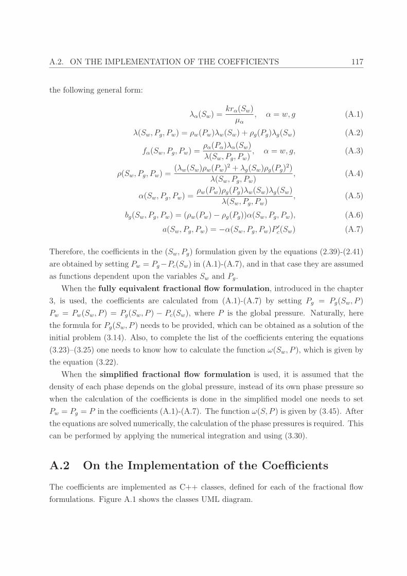
A.2. ON THE IMPLEMENTATION OF THE COEFFICIENTS 117
the following general form:
λα(Sw) =krα(Sw)
µα
, α = w, g (A.1)
λ(Sw, Pg, Pw) = ρw(Pw)λw(Sw) + ρg(Pg)λg(Sw) (A.2)
fα(Sw, Pg, Pw) =ρα(Pα)λα(Sw)
λ(Sw, Pg, Pw), α = w, g, (A.3)
ρ(Sw, Pg, Pw) =(λw(Sw)ρw(Pw)2 + λg(Sw)ρg(Pg)
2)
λ(Sw, Pg, Pw), (A.4)
α(Sw, Pg, Pw) =ρw(Pw)ρg(Pg)λw(Sw)λg(Sw)
λ(Sw, Pg, Pw), (A.5)
bg(Sw, Pg, Pw) = (ρw(Pw) − ρg(Pg))α(Sw, Pg, Pw), (A.6)
a(Sw, Pg, Pw) = −α(Sw, Pg, Pw)P ′
c(Sw) (A.7)
Therefore, the coefficients in the (Sw, Pg) formulation given by the equations (2.39)-(2.41)
are obtained by setting Pw = Pg−Pc(Sw) in (A.1)-(A.7), and in that case they are assumed
as functions dependent upon the variables Sw and Pg.
When the fully equivalent fractional flow formulation, introduced in the chapter
3, is used, the coefficients are calculated from (A.1)-(A.7) by setting Pg = Pg(Sw, P )
Pw = Pw(Sw, P ) = Pg(Sw, P ) − Pc(Sw), where P is the global pressure. Naturally, here
the formula for Pg(Sw, P ) needs to be provided, which can be obtained as a solution of the
initial problem (3.14). Also, to complete the list of the coefficients entering the equations
(3.23)–(3.25) one needs to know how to calculate the function ω(Sw, P ), which is given by
the equation (3.22).
When the simplified fractional flow formulation is used, it is assumed that the
density of each phase depends on the global pressure, instead of its own phase pressure so
when the calculation of the coefficients is done in the simplified model one needs to set
Pw = Pg = P in the coefficients (A.1)-(A.7). The function ω(S, P ) is given by (3.45). After
the equations are solved numerically, the calculation of the phase pressures is required. This
can be performed by applying the numerical integration and using (3.30).
A.2 On the Implementation of the Coefficients
The coefficients are implemented as C++ classes, defined for each of the fractional flow
formulations. Figure A.1 shows the classes UML diagram.

A.2. ON THE IMPLEMENTATION OF THE COEFFICIENTS 118
FractFlowFun<TPF,FP>
FractFlowFunBase
ParametersBase
Parameters<A,B>
GPExactFractFlow
Fun<TPF,FP>GPSimplFractFlow
Fun <TPF,FP>
GlobalExactTables
<TPF,FP>GlobalSimplTables
<TPF,FP>
pr
pr
table
table table
table
GlobalTables
Figure A.1: UML diagram for the coefficients
The implementation is centered on the FractFlowFunBase class. This is the base class
providing an interface for the two-phase flow (TPF) and fluid properties (FP) functions.
All the coefficients implementations take two arguments:
• Wetting phase saturation (that can be switched to capillary pressure)
• Pressure.
In this class, all the coefficients are defined as pure virtual functions.
The class StaticFractFlowFun is an auxiliary class used to implement formulae for
the coefficients (A.1)-(A.7) and their partial derivatives as static functions. It is written
as a template parametrized by the classes implementing TPF and FP. It contains all the
coefficients, as the FractFlowFunBase class. For this class, note that the relevant functions
had to be implemented as static, because of the requirements of GSL library [45] used in
GlobalExactTables class.
The class FractFlowFun inherits the abstract class FractFlowFunBase. This class is
implemented as a template parametrized by the TPF and FP classes. The pure virtual
A.2. ON THE IMPLEMENTATION OF THE COEFFICIENTS 119
functions from the abstract FractFlowFunBase class are implemented here as virtual func-
tions, depending on the wetting phase saturation and the nonwetting phase pressure as is
presented in the formulae (2.33)-(2.37). These functions subsequently rely on the functions
implemented in the classes TPF, FP and StaticFractFlowFun. So, the coefficient func-
tions in the FractFlowFun<TPF,FP> class are implemented by calling the functions from
StaticFractFlowFun class taking as arguments wetting phase saturation and the values
of the virtual functions Pn (S,P) and Pw (S,P), which will be defined separately for each
class inheriting the FractFlowFun<TPF,FP> class. In the class FractFlowFun<TPF, FP> is
set to be
Pn (S,P) = P (A.8)
Pw (S,P) = P − Pc(S), (A.9)
so, here the unknown P is assumed to be the gas pressure.
The class FractFlowFun<TPF,FP> also contains an object pr of the type Parameters.
This object provides the parameters for the TPF and FP classes. As an example of the
required parameters, van Genuchten’s functions require parameters: Pr, n, residual satura-
tion of wetting and nonwetting phase and the parameters for linearization of the capillary
pressure. The task of the Parameters object is to store all the required parameters.
The GPExactFractFlowFun<TPF,FP> clas inherits the FractFlowFun<TPF,FP> class.
This class implements the coefficients for the fully equivalent global pressure formulation.
The following is set:
Pn (S,P) = Pg(S,P) (A.10)
Pw (S,P) = Pg(S,P) − Pc(S). (A.11)
The nonwetting phase pressure Pg(S, P ) and the function ω(S, P ) are calculated from the
object table of the type GlobalExactTables<TPF,FP>.
The GPSimplFractFlowFun<TPF,FP> inherits the class FractFlowFun<TPF,FP> by set-
ting:
Pn (S,P) = P (A.12)
Pw (S,P) = P. (A.13)
This class implements the coefficients for the simplified global pressure fractional flow for-
A.2. ON THE IMPLEMENTATION OF THE COEFFICIENTS 120
mulation. The nonwetting phase pressure Pg(S, P ) and the function ω(S, P ) are calculated
from the object table of the type GlobalSimplTables<TPF,FP>.
The class GlobalExactTables<TPF,FP> implements a look-up table for the values of
Pg(S, P ). For each value of the global pressure vector in a certain range (values ranging
from Pmin to Pmax), Pg(u, P ) is calculated as a solution of the initial problem (3.15). The
calculation is performed by using a GSL ODE solver. This class also provides a table of
values for the functionω(S, P ). The function Pg(S, P ) and ω(S, P ) are calculated from the
corresponding tables by linear interpolation.
The class GlobalSimplTables<TPF,FP> performs the equivalent task for the simplified
coefficients case - it provides the calculation of Pg(S, P ). The difference is that, in this
case, the tables are obtained by numerical integration.
The function of these two classes storing the tables is to calculate the required values
only once at the beginning of each numerical simulation. When required in the later phase,
the values are only looked up in the tables. For a large pressure range, this is obviously a
very memory-intensive task.
The TPF classes contain relative permeabilities functions, capillary pressure and their
derivatives. Currently, the implemented classes are VanGenuchtenFun, BrooksCoreyFun,
SimpleFun (krw(Sw) = S2w, krg(Sw) = (1 − Sw)2, Pc(Sw) = Pr(1 − Sw)). The variable in
TPF class can be switched to the capillary pressure or the wetting phase saturation, so
consequently all the coefficients can depend either on the wetting phase saturation or on
the capillary pressure.
The examples of the FP classes are class FluidCompress which models densities as
exponential functions, and FluidCompInc which models flow of water and gas (the density
is given by the gas ideal law).
Bibliography
[1] M. Afif, Schemas Volumes finis pour une Classe d’Equations de Type Convection-
Diffusion Issues des Milieux Poreux, These, Universite Cadi Ayyad, (2002).
[2] M. Afif, B. Amaziane, On convergence of finite volume schemes for one-dimensional
two-phase flow in porous media, J. Comput. Appl. Math. 145 (2002) 31–48.
[3] M. Afif, B. Amaziane, Convergence of finite volume schemes for a degenerate
convection–diffusion equation arising in flow in porous media, Comput. Methods Appl.
Mech. Engrg., 191 (2002) 5265-5286.
[4] M. Afif, B. Amaziane, Numerical simulation of two-phase flow through heerogeneous
porous media, Numer. Algorithms, 34 (2003) 117-125.
[5] M. Afif, B. Amaziane, Convergence of a 1-D finite volume scheme and numerical sim-
ulations for water-gas flow in porous media, Preprint submitted to Applied Numerical
Mathematics (2010).
[6] H.W. Alt, E. Di Benedetto, Nonsteady flow of water and oil through inhomogeneous
porous media, Ann. Scu. Norm. Sup. Pisa Cl. Sci. 12 (4) (1985) 335–392.
[7] B. Amaziane, M. Jurak, A new formulation of immiscible compressible two-phase flow
in porous media, C. R. Mecanique 336 (2008) 600-605.
[8] B. Amaziane, M. Jurak, A. Zgaljic Keko, Modeling and numerical simulations of
immiscible compressible two-phase flow in porous media by the concept of global
pressure, Transport in Porous Media 84 (2010) 133-152.
[9] B. Amaziane, M. Jurak, A. Zgaljic Keko, An existence result for a coupled system
modeling a fully equivalent global pressure formulation for immiscible compressible
two-phase flow in porous media, Journal of Differential Equations 250 (2011), 1685-
1718.
[10] Y. Amirat, K. Hamdache, A. Ziani, Mathematical analysis for compressible miscible
displacement models in porous media, Math. Models Methods Appl. Sci. 6 (6) (1996)
729–747.
[11] Y. Amirat, M. Moussaoui, Analysis of a one-dimensional model for compressible mis-
cible displacement in porous media, SIAM J. Math. Anal. 26 (3) (1995) 659–674.
[12] Y. Amirat, V. Shelukhin, Global weak solutions to equations of compressible miscible
flows in porous media, SIAM J. Math. Anal. 38 (6) (2007) 1825–1846.
[13] ANDRA: Couplex-Gaz (2006). Available online at
http://www.gdrmomas.org/ex qualifications.html (2006).
[14] O. Angelini, C. Chavant, E. Chenier, R. Eymard, S. Granet, Finite volume approx-
imation of a diffusion-dissolution model and application to nuclear waste storage,
Mathematics and Computers in Simulation (2010), in press
[15] S.N. Antontsev, A.V. Kazhikhov, V.N. Monakhov, Boundary Value Problems in Me-
chanics of Nonhomogeneous Fluids, North-Holland, Amsterdam, (1990).
[16] T. Arbogast, The existence of weak solutions to single-porosity and simple dual-
porosity models of two-phase incompressible flow, Nonlinear Anal. 19 (11) (1992)
1009–1031.
[17] P. Bastian, Numerical Computation of Multiphase Flows in Porous Meadia, Habilita-
tionsschrift, 1999.
[18] J. Bear, Y. Bachmat, Introduction to Modeling of Transport Phenomena in Porous
Media, Kluwer Academic Publishers, London, 1991.
[19] J. Bear, A. Verruijt, Introduction to Modeling Groundwater Flow and Pollution, D.
Reidel Publishing Company, Dordrecht, Holland,1987.
[20] A. Bourgeat, A. Hidani, A result of existence for a model of two-phase flow in a porous
medium made of different rock types, Appl. Anal. 56 (1995) 381–399.
[21] A. Bourgeat, M. Jurak, F. Smaı, Two-phase, partially miscible flow and transport
modeling in porous media; application to gas migration in a nuclear waste repository,
Comput. Geosci. 13 (2009), no. 1, 29-42.
[22] R.H. Brooks, A.T. Corey, Properties of porous media affecting fluid flow, J. Irrig. and
Drainage Div., Proc. ASCE, Vol 92, IR2, 61-88
[23] R.H. Brooks, A.T. Corey, Hydraulic properties of porous media, Colorado State Uni-
versity Hydrology Paper No.3, March, 27p
[24] G. Chavent, A fully equivalent global pressure formulation for three-phases compress-
ible flows, Appl. Anal. 88 (10–11) (2009) 1527–1541.
[25] G. Chavent, J. Jaffre, Mathematical Models and Finite Elements for Reservoir Simu-
lation, North–Holland, Amsterdam, 1986.
[26] J.Chen, J.W. Hopmans, M.E. Grismer, Parameter estimation of two-fluid capillary
pressure–saturaion and permeability functions
[27] Z. Chen, Degenerate two-phase incompressible flow I: Existence, uniqueness and reg-
ularity of a weak solution, J. Differential Equations 171 (2) (2001) 203–232.
[28] Z. Chen, R.E. Ewing, From single-phase to compositional flow: Applicability of mixed
finite elements, Transport in Porous Media 27 (1997) 225–242.
[29] Z. Chen, R.E. Ewing,: Comparison of various formulations of three-phase flow in
porous media, J. Comp. Physics, 132 (1997), 362–373.
[30] Z. Chen, G. Huan, Y. Ma, Computational Methods for Multiphase Flows in Porous
Media, SIAM, Philadelphia, 2006.
[31] R. di Chiara Roupert, Developpement d’un code de calcul multiphasique multiconsti-
tuants, these, Universite de Strasbourg (2009).
[32] R. di Chiara Roupert, G. Chavent, G. Schafer, Three-phase compressible flow in
porous media : Total Differential Compatible interpolation of relative permeabilities,
Journal of Computational Physics 229 (2010), 4762-4780.
[33] R. di Chiara Roupert, G. Schafer, P. Ackerer, M. Quintard, G. Chavent, Construc-
tion of three-phase data to model multiphase flow in porous media: Comparing
an optimization approach to the finite element approach, C.R. Geoscience (2010),
doi:10.1016/j.crte.2010.07.004
[34] C. Choquet, On a fully coupled nonlinear parabolic problem modelling miscible com-
pressible displacement in porous media, J. Math. Anal. Appl. 339 (2) (2008) 1112–
1133.
[35] A.T. Corey, Mechanics of immiscible fluids in porous media, Water Resources Publi-
cations, Highlands Ranch,Colorado, USA, 1994
[36] F.Z. Daım, R. Eymard, D. Hilhorst, Existence of a solution for two phase flow in
porous media: the case that the porosity depends on the pressure, J. Math. Anal.
Appl. 326 (2007) 332–351.
[37] C.J. van Dujin, M.J. de Neef, Similarity solution for capillary redistribution of two
phases in a porous medium with a single discontinuity, Advances in Water Resources
21 (1998), 451-461.
[38] B.K. Fadimba, On existence and uniqueness for a coupled system modeling immiscible
flow through a porous medium, J. Math. Anal. Appl. 328 (2007) 1034–1056.
[39] X. Feng, Strong solutions to a nonlinear parabolic system modeling compressible mis-
cible displacement in porous media, Nonlinear Anal. 23 (12) (1994) 1515–1531.
[40] G. Gagneux, M. Madaune-Tort, Analyse Mathematique de Modeles Non Lineaires de
l’Ingenierie Petroliere, Springer-Verlag, Berlin, 1996.
[41] C. Galusinski, M. Saad, On a degenerate parabolic system for compressible, immis-
cible, two-phase flows in porous media, Adv. Differential Equations 9 (11–12) (2004)
1235–1278.
[42] C. Galusinski, M. Saad, A nonlinear degenerate system modelling water-gas flows in
porous media, Discrete Contin. Dyn. Syst. Ser. B 9 (2) (2008) 281–308.
[43] C. Galusinski, M. Saad, Two compressible immiscible fluids in porous media, J. Dif-
ferential Equations 244 (7) (2008) 1741–1783.
[44] C. Galusinski, M. Saad, Weak solutions for immiscible compressible multifluid flows
in porous media, C. R. Math. Acad. Sci. Paris 347 (5–6) (2009) 249–254.
[45] GSL-GNU Scientific Library, http://www.gnu.org/software/gsl/
[46] R. Helmig, Multiphase Flow and Transport Processes in the Subsurface, Springer,
Berlin (1997).
[47] R. Huber, R. Helmig, Node-centered finite volume discretizations for the numeri-
cal simulation of multiphase flow in heterogeneous porous media, Comput. Geosci. 4
(2000), no. 2, 141-164.
[48] Z. Khalil, M. Saad, Solution to a model for compressible immiscible two phase flow in
porous media, Electron.j. Differential Equations 122 (2010), 1-33.
[49] D. Kroner, S. Luckhaus, Flow of oil and water in a porous medium, J. Differential
Equations 55 (2) (1984) 276–288.
[50] LibMesh library, http://libmesh.sourceforge.net/index.php
[51] A. Mikelic, An existence result for the equations describing a gas–liquid two–phase
flow, C. R. Mecanique 337 (2009) 226–232.
[52] MoMaS - Exercices de Qualification Numerique de Codes,
http://www.gdrmomas.org/ex qualifications.html
[53] H.J. Morel-Seytoux, P.D. Meyer, M. Nachabr, J. Touma, M.T. van Genuchten, R.J.
Lenhard, Parameter equivalance for the Brooks-Corey and van Genuchten soil charac-
teristics: Preserving the effective capillary drive, water resoureces research 32 (1996),
1251-1258.
[54] D. Nayagum, G. Schafer, R. Mose, Modelling two-phase incompressible flow in porous
media using mixed hybrid and discontinuous finite elements, Computational Geo-
sciences 8 (2004), 49-73.
[55] M.J. de Neef, J. Molenaar, Analysis of DNAPL infiltration in a medium with a low-
permeable lens, Computational Geosciences 1 (1997) 191–214.
[56] J. Niessner, R. Helmig, H. Jakobs, J.E. Roberts, Interface condition and linearization
schemes in the Newton iterations for two-phase flow in heterogeneous porous media,
Advances in Water Resources 28 (2005) 671-687.
[57] OECD/NEA, Safety of Geological Disposal of High-level and Long-lived Radioactive
Waste in France, An International Peer Review of the “Dossier 2005 Argile” Concern-

ing Disposal in the Callovo-Oxfordian Formation. OECD Publishing (2006). Available
online at http://www.nea.fr/html/rwm/reports/2006/nea6178-argile.pdf
[58] M. Ohlberger, Convergence of a mixed finite element-finite volume methods for two
phase flow in porous media, East-West J. Numer. Math. 5 (1997), 183-210.
[59] A. Papafotiou, H. Sheta, R. Helmig, Numerical modeling of two-phase hysteresis com-
bined with an interface condition for heterogeneous porous media, Computational
Geosciencs 14 (2010) 273–287.
[60] J. Simon, Compact sets in the space Lp(O, T ;B), Ann. Mat. Pura Appl. 146 (4) (1987)
65–96.
[61] F. Smaı, Developpement d’outils mathematiques et numeerigues pour l’evaluation du
concept de stockage geologique, these, Universite de Lyon (2009).
[62] F. Smaı, A model of multiphase flow and transport in porous media applied to gas
migration in underground nuclear waste repository, C. R. Math. Acad. Sci. Paris 347
(9–10) (2009) 527–532.
[63] F. Smaı, Existence of solutions for a model of multiphase flow in porous media applied
to gas migration in underground nuclear waste repository, Appl. Anal. 88 (10–11)
(2009) 1609–1616.
[64] M. van Genuchten, A closed-form equation for predicting the hydraulic conductivity
of unsaturated soils, Soil Sci. Soc. Am.J 44 (1980) 892-898.
[65] C.Y. Wang, An alternative description of viscous coupling in two-phase flow through
porous media, Transport in Porous Media 28 (1997) 205–219.
[66] L.M. Yeh, On two-phase flow in fractured media, Math. Models Methods Appl. Sci.
12 (8) (2002) 1075–1107.
[67] L.M. Yeh, Holder continuity for two-phase flows in porous media, Math. Methods
Appl. Sci. 29 (11) (2006) 1261–1289.
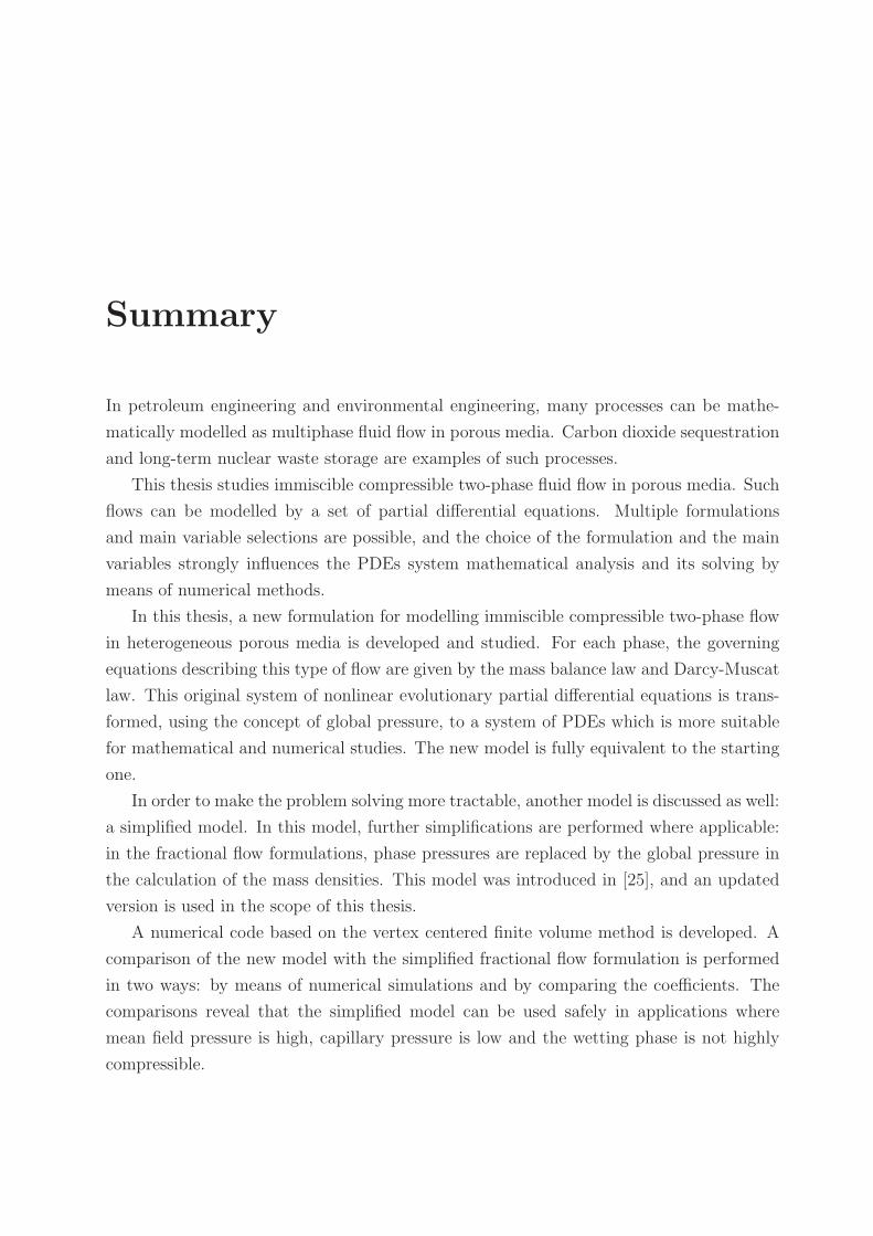
Summary
In petroleum engineering and environmental engineering, many processes can be mathe-
matically modelled as multiphase fluid flow in porous media. Carbon dioxide sequestration
and long-term nuclear waste storage are examples of such processes.
This thesis studies immiscible compressible two-phase fluid flow in porous media. Such
flows can be modelled by a set of partial differential equations. Multiple formulations
and main variable selections are possible, and the choice of the formulation and the main
variables strongly influences the PDEs system mathematical analysis and its solving by
means of numerical methods.
In this thesis, a new formulation for modelling immiscible compressible two-phase flow
in heterogeneous porous media is developed and studied. For each phase, the governing
equations describing this type of flow are given by the mass balance law and Darcy-Muscat
law. This original system of nonlinear evolutionary partial differential equations is trans-
formed, using the concept of global pressure, to a system of PDEs which is more suitable
for mathematical and numerical studies. The new model is fully equivalent to the starting
one.
In order to make the problem solving more tractable, another model is discussed as well:
a simplified model. In this model, further simplifications are performed where applicable:
in the fractional flow formulations, phase pressures are replaced by the global pressure in
the calculation of the mass densities. This model was introduced in [25], and an updated
version is used in the scope of this thesis.
A numerical code based on the vertex centered finite volume method is developed. A
comparison of the new model with the simplified fractional flow formulation is performed
in two ways: by means of numerical simulations and by comparing the coefficients. The
comparisons reveal that the simplified model can be used safely in applications where
mean field pressure is high, capillary pressure is low and the wetting phase is not highly
compressible.
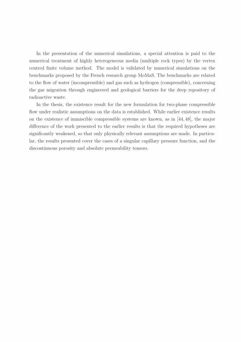
In the presentation of the numerical simulations, a special attention is paid to the
numerical treatment of highly heterogeneous media (multiple rock types) by the vertex
centred finite volume method. The model is validated by numerical simulations on the
benchmarks proposed by the French research group MoMaS. The benchmarks are related
to the flow of water (incompressible) and gas such as hydrogen (compressible), concerning
the gas migration through engineered and geological barriers for the deep repository of
radioactive waste.
In the thesis, the existence result for the new formulation for two-phase compressible
flow under realistic assumptions on the data is established. While earlier existence results
on the existence of immiscible compressible systems are known, as in [44, 48], the major
difference of the work presented to the earlier results is that the required hypotheses are
significantly weakened, so that only physically relevant assumptions are made. In particu-
lar, the results presented cover the cases of a singular capillary pressure function, and the
discontinuous porosity and absolute permeability tensors.
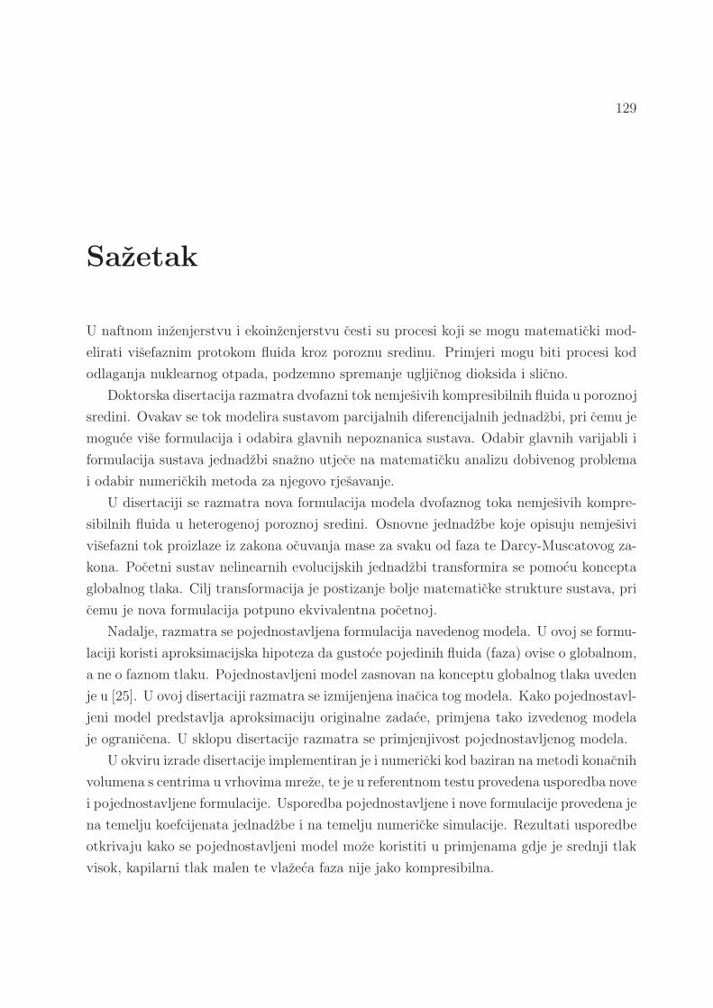
129
Sazetak
U naftnom inzenjerstvu i ekoinzenjerstvu cesti su procesi koji se mogu matematicki mod-
elirati visefaznim protokom fluida kroz poroznu sredinu. Primjeri mogu biti procesi kod
odlaganja nuklearnog otpada, podzemno spremanje ugljicnog dioksida i slicno.
Doktorska disertacija razmatra dvofazni tok nemjesivih kompresibilnih fluida u poroznoj
sredini. Ovakav se tok modelira sustavom parcijalnih diferencijalnih jednadzbi, pri cemu je
moguce vise formulacija i odabira glavnih nepoznanica sustava. Odabir glavnih varijabli i
formulacija sustava jednadzbi snazno utjece na matematicku analizu dobivenog problema
i odabir numerickih metoda za njegovo rjesavanje.
U disertaciji se razmatra nova formulacija modela dvofaznog toka nemjesivih kompre-
sibilnih fluida u heterogenoj poroznoj sredini. Osnovne jednadzbe koje opisuju nemjesivi
visefazni tok proizlaze iz zakona ocuvanja mase za svaku od faza te Darcy-Muscatovog za-
kona. Pocetni sustav nelinearnih evolucijskih jednadzbi transformira se pomocu koncepta
globalnog tlaka. Cilj transformacija je postizanje bolje matematicke strukture sustava, pri
cemu je nova formulacija potpuno ekvivalentna pocetnoj.
Nadalje, razmatra se pojednostavljena formulacija navedenog modela. U ovoj se formu-
laciji koristi aproksimacijska hipoteza da gustoce pojedinih fluida (faza) ovise o globalnom,
a ne o faznom tlaku. Pojednostavljeni model zasnovan na konceptu globalnog tlaka uveden
je u [25]. U ovoj disertaciji razmatra se izmijenjena inacica tog modela. Kako pojednostavl-
jeni model predstavlja aproksimaciju originalne zadace, primjena tako izvedenog modela
je ogranicena. U sklopu disertacije razmatra se primjenjivost pojednostavljenog modela.
U okviru izrade disertacije implementiran je i numericki kod baziran na metodi konacnih
volumena s centrima u vrhovima mreze, te je u referentnom testu provedena usporedba nove
i pojednostavljene formulacije. Usporedba pojednostavljene i nove formulacije provedena je
na temelju koefcijenata jednadzbe i na temelju numericke simulacije. Rezultati usporedbe
otkrivaju kako se pojednostavljeni model moze koristiti u primjenama gdje je srednji tlak
visok, kapilarni tlak malen te vlazeca faza nije jako kompresibilna.
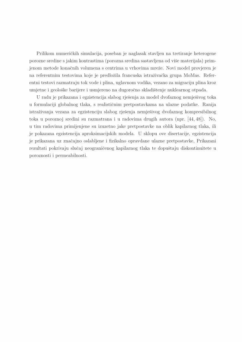
Prilikom numerickih simulacija, poseban je naglasak stavljen na tretiranje heterogene
porozne sredine s jakim kontrastima (porozna sredina sastavljena od vise materijala) prim-
jenom metode konacnih volumena s centrima u vrhovima mreze. Novi model provjeren je
na referentnim testovima koje je predlozila francuska istrazivacka grupa MoMas. Refer-
entni testovi razmatraju tok vode i plina, uglavnom vodika, vezano za migraciju plina kroz
umjetne i geoloske barijere i usmjereno na dugorocno skladistenje nuklearnog otpada.
U radu je prikazana i egzistencija slabog rjesenja za model dvofaznog nemjesivog toka
u formulaciji globalnog tlaka, s realisticnim pretpostavkama na ulazne podatke. Ranija
istrazivanja vezana za egzistenciju slabog rjesenja nemjesivog dvofaznog kompresibilnog
toka u poroznoj sredini su razmatrana i u radovima drugih autora (npr. [44, 48]). No,
u tim radovima primijenjene su izuzetno jake pretpostavke na oblik kapilarnog tlaka, ili
je pokazana egzistencija aproksimacijskih modela. U sklopu ove disertacije, egzistencija
je prikazana uz znacajno oslabljene i fizikalno opravdane ulazne pretpostavke, Prikazani
rezultati pokrivaju slucaj neogranicenog kapilarnog tlaka te dopustaju diskontinuitete u
poroznosti i permeabilnosti.

131
Curriculum Vitae
Ana Zgaljic Keko was born in Rijeka, Croatia, on 8 June, 1980. After obtaining secondary
education in Krk, she started the undergraduate studies of Applied Mathematics at the
Faculty of Science, University of Zagreb in 1998, where she graduated in 2004. In the same
year, she started the postgraduate studies at the same faculty. Starting with 2005, she
works as a teaching and research assistant at the Faculty of Electrical Engineering and
Computing at the University of Zagreb.
132
Zivotopis
Ana Zgaljic Keko rodena je u Rijeci 8. lipnja 1980. godine. Osnovnu i srednju skolu zavrsila
je u Krku. Prirodoslovno-matematicki fakultet Sveucilista u Zagrebu upisuje 1998. godine
i 2004. godine zavrsava studij matematike, smjer primijenjena matematika. Iste godine
upisuje poslijediplomski znanstveni studij matematike na istom fakultetu. Od 2005. godine
zaposlena je kao asistent na Zavodu za primijenjenu matematiku Fakulteta elektrotehnike
i racunarstva Sveucilista u Zagrebu.