modelling adult mortality in small - demografi · modelling adult mortality in small populations:...

MODELLING ADULT MORTALITY IN SMALLPOPULATIONS: THE SAINT MODEL

SØREN FIIG JARNER AND ESBEN MASOTTI KRYGER

Abstract. The mortality evolution of small populations often exhibitssubstantial variability and irregular improvement patterns making ithard to identify underlying trends and produce plausible projections.We propose a methodology for robust forecasting based on the existenceof a larger reference population sharing the same long-term trend as thepopulation of interest. The reference population is used to estimatethe parameters in a frailty model for the underlying intensity surface.A multivariate time series model describing the deviations of the smallpopulation mortality from the underlying mortality is then tted andforecasted. Coherent long-term forecasts are ensured by the underlyingfrailty model while the size and variability of short- to medium-termdeviations are quantied by the time series model. The frailty model isparticularly well suited to describe the changing improvement patternsin old age mortality. We apply the method to Danish mortality datawith a pooled international data set as reference population.

1. IntroductionMortality projections are of great importance for public nancing deci-

sions, health care planning and the pension industry. A large number offorecasts are being produced on a regular basis by government agencies andpension funds for various populations of interest. In many situations thepopulation of interest is quite small, e.g. the population of a small region orthe members of a specic pension fund, and historic data shows substantialvariability and irregular patterns. Also, historic data may be available onlyfor a relatively short period of time.

The prevailing methodology for making mortality projections is the methodproposed by Lee and Carter (1992). The model describes the evolution inage-specic death rates (ASDRs) by a single time-varying index togetherwith age-specic responses to the index. The structure implies that all AS-DRs move up and down together, although not by the same amounts. Themethod has gained widespread popularity due to its simplicity and ease of in-terpretation and there has been a wealth of applications, see e.g. Tuljapurkaret al. (2000); Booth et al. (2006) and references therein. A number of exten-sions and improvements have been proposed, e.g. Brouhns et al. (2002); Lee

Date: December 2, 2008.Key words and phrases. SAINT model, stochastic modelling, small populations, adult

mortality, frailty, changing rates of improvement, Danish and international mortality.1

2 SØREN FIIG JARNER AND ESBEN MASOTTI KRYGER

and Miller (2001); Renshaw and Haberman (2006); Renshaw and Haberman(2003); de Jong and Tickle (2006); Currie et al. (2004); Cairns et al. (2006),but the original Lee-Carter method still serves as the point of reference.

1.1. Small population mortality. The structure of the Lee-Carter modelmakes it well suited to extrapolate regular patterns with constant improve-ment rates over time. However, while the mortality experience of large pop-ulations often conforms with this pattern the mortality evolution of smallpopulations is generally much more irregular. Lack of t of the Lee-Cartermodel for small populations, including the Nordic countries, was reportedby Booth et al. (2006) in a comparative study. In Denmark, for instance,improvement rates have varied considerably over time within age groups andthere has been periods with improvements in some age groups and stagna-tion or even slight increases in other age groups violating the Lee-Carterassumptions; see Jarner et al. (2008); Andreev (2002) for detailed accountsof the evolution of Danish mortality.

The characteristics of small population mortality makes forecasting basedon past trends problematic and very sensitive to the tting period. Naiveextrapolation of historic trends in ASDRs is likely to lead to implausibleprojections and unrealistic age-proles, e.g. old age mortality dropping belowthat of younger ages. Often, however, the population under study can beregarded as a subpopulation of a (larger) reference population obeying amore regular pattern of improvement, e.g. a region within a country, or asmall country in a larger geographical area etc. Furthermore, it will oftenbe reasonable to assume that the study and reference populations will sharethe same long-term trend.

In this paper we propose a methodology for robust small population mor-tality projection based on the identication of a reference population. Themethod consists of two steps: First, the reference population is used to esti-mate a parametric, underlying intensity surface which determines the long-term trend. Second, a multivariate, stationary time series model describingthe deviations of the small population mortality from the trend is tted. Pro-jections are obtained by combining extrapolations of the parametric surfacewith forecasts of the time series model for deviations. Coherent long-termmortality proles are guaranteed by the parametric surface while the pur-pose of the time series is to quantify the short- to medium-term variabilityin improvement rates of the small population.

It is common to base mortality forecasts on time series models. Typi-cally, parameters describing the evolution of period life tables are estimatedassuming either a parametric or non-parametric age-prole. A time seriesmodel, often a random-walk with drift, is then tted and forecasted for eachof the parameters. The role of the time series in these methods is to cap-ture both the trend in parameters and their uncertain evolvement aroundthe trend. The structure implies that large short-term variability invariablylead to even larger long-term variability. In contrast, the proposed method

MODELLING ADULT MORTALITY IN SMALL POPULATIONS: THE SAINT MODEL 3

by treating deviations from the trend as stationary allows for substantialshort-term variability without inating the long-term uncertainty.

1.2. Old age mortality. The modelling of old age mortality presents per-haps the most challenging part of mortality modelling. The historic develop-ment in Danish old age mortality, say age 70 and above, shows very modestimprovement rates, far below those observed for the younger ages. However,over the last decade or so improvement rates have picked up and currently70-year-olds experience improvement rates equalling those of younger ages.The picture is the same in most developed countries: old age mortality hashistorically improved at a slower pace than young and middle age mortality,but recently improvements rates have gradually risen.

The fact that old age improvement rates increase over time cause forecastsbased on the Lee-Carter methodology to systematically under-predict thegains in old age mortality, cf. Lee and Miller (2001). As a consequence it hasbeen recommended to use a shorter tting period over which data conformsbetter with the assumptions of time-invariant improvement rates, see e.g. Leeand Miller (2001); Tuljapurkar et al. (2000); Booth et al. (2002). Althoughthis approach clearly forecasts higher improvement rates in old age mortalityit seems somewhat ad-hoc and not entirely satisfying. In this paper we takea dierent route.

Our ambition is to derive a simple model for the population dynamicsin which changing mortality patterns naturally arise. This will allow us tocharacterize how mortality improvements change over time and to make pre-dictions for future improvements in old and oldest-old mortality. Inspiredby frailty theory we assume that the population consists of a heterogeneousgroup of individuals with varying degrees of frailty. Frail individuals havea tendency to die rst causing a concentration of robust individuals at highages. Taken this selection mechanism into account and assuming continuedimprovements over time a model for the entire intensity surface of the popu-lation over time can be derived. We will use the resulting parametric surfaceto describe the development of the reference population.

The frailty model oers an explanation to the observed lack of improve-ment in old age mortality. The mortality for a given age group at a giventime is inuenced by two factors: the current level of health and the aver-age frailty. Over time the level of health improves but so does the averagefrailty. In eect, as mortality improves the selection mechanism to reacha given age weakens causing healthier but more frail individuals to becomeold. In the transition from high to low selection the two eects partly oseteach other such that the aggregate mortality for the age group is almostconstant. Eventually the health eect will dominate the selection eect andimprovements will be seen. We will explore these eects in some detail andderive the asymptotic improvement pattern implied by the model.

For two reasons we focus on adult mortality only in our modelling, i.e.mortality for age 20 and above. First, the nature of infant and child mortality


is rather dierent from adult mortality and more complexity will have to beadded to the model to t the historic evolution adequately. Second, currentlevels of infant and child mortality are so low that their future course has verylittle impact on life expectancy and other aggregate measures. Hence, froma forecasting perspective not much is gained by the added complexity. Infact, with current mortality levels already very low up to age 60, say, futurelife expectancy gains will be driven almost exclusively by the developmentin old age mortality. However, by modelling the full adult mortality surfacewe are able to extract information about the general nature of improvementpatterns and to predict when improvements will start to occur for age groupswhere none have been seen historically.

1.3. Outline. The rest of the paper is organized as follows: in Section 2.1 wepresent the proposed methodology for small population mortality modellingconsisting of a separation of trends and deviations; in Section 2.2 we derivea parametric, frailty model for the underlying intensity surface and studysome implications and asymptotic properties; and Section 2.3 contains adescription of the time series model for deviations. In Section 3 we give anapplication to Danish data taken a large international data set as referencepopulation, Section 4 contains a study of the t and forecasting performanceof the model, and in Section 5 we oer some concluding remarks and indicatefurther lines of research. All proofs are in the Appendix.

2. The model2.1. Methodology. In the following we suggest a methodology for robustforecasting of small population mortality. The evolution of small populationmortality is characterized by being more volatile and having less regularimprovement patterns compared to what is observed in larger populations.These features make simple projection methodologies very sensitive to thechoice of tting period and lead to very uncertain long-term forecasts. Thefundamental idea in the proposed method is to use a large population toestimate the underlying long-term trend and use the small population toestimate the deviations from the trend.

We distinguish between unsystematic and systematic variability. Unsys-tematic variability refers to the variability associated with the randomnessof the time of deaths in a population with a known mortality intensity, whilesystematic variability refers to the variability of the mortality intensity it-self. Since the populations we are interested in are small by assumption weexpect noticeable unsystematic variability. For instance, we do not expectcrude (unsmoothed) death rates, constructed from the mortality experienceof a single year, to be strictly increasing with age although we believe it tohold for the underlying intensity (at least from some age).

However, even taken the larger unsystematic variability into account itappears that small populations also have a greater systematic variability


than larger populations. Presumably small populations are more homoge-neous and thereby more inuenced by specic eects. There are a numberof reasons why this might be. Consider for instance the members of an occu-pational pension scheme. The members have the same or similar educationand job, and probably also to some extent similar economic status and lifestyle compared to the population at large. Similarly, the population in aspecic country is inuenced by common factors, e.g. the health care systemand social habits such as smoking. The homogeneity implies that specicchanges in e.g. socioeconomic conditions will have a greater impact on themortality in a small population compared to a large population with greaterdiversity in background factors.

We will assume that the population under study can be regarded as asubpopulation of a larger population, e.g. the population of a province isa subpopulation of the national population, and a national population canbe regarded a subpopulation of the total population of a larger geograph-ical region, or of similarly developed countries. We will refer to the smallpopulation as the subpopulation and the large population as the referencepopulation. Although both unsystematic and systematic variability will begreater in the subpopulation it is reasonable to assume that the sub- and ref-erence populations will share the same long-term trends in mortality decline,even in the presence of substantial deviations in current mortality levels. Thealternative is diverging levels of mortality which in the long run seems highlyunlikely for related populations. Wilson (2001); Wilmoth (1998) provide ev-idence for convergence in global mortality levels due to convergence of socialand economic factors.

2.1.1. Data. We will assume that data consists of death counts, D(t, x),and corresponding exposures, E(t, x), for a range of years t and ages x.Data is assumed to be available for both the sub- and reference population(distinguished by subscript sub and ref, respectively), but not necessarily forthe same ranges of years and ages. Data will typically also be gender specic,but it does not have to be. Since it is of no importance for the formulationof the model we will suppress a potential gender dependence in the notation.

D(t, x) denotes the number of deaths occurring in calender year t amongpeople aged [x, x + 1), and E(t, x) denotes the total number of years livedduring calender year t by people of age [x, x + 1). For readers familiarwith the Lexis diagram, D(t, x) counts the number of deaths in the square[t, t+1)× [x, x+1) of the Lexis diagram and E(t, x) gives the correspondingexposure, i.e. we work with so-called A-groups.

2.1.2. Model structure. From the death counts and exposures we can formthe (crude) death rates

(1) m(t, x) =D(t, x)E(t, x)

,


which are estimates of the underlying intensity, or force of mortality, µ(t, x)1.In order to proceed we assume that we have a family of intensity surfaces

Hθ(t, x) parameterized by θ, and we consider the model where death countsare independent with(2) Dref(t, x) ∼ Poisson (µref(t, x)Eref(t, x)) ,

and µref(t, x) = Hθ(t, x). Based on this model we nd the maximum like-lihood estimate (MLE) for θ, denoted by θ. In principle we could use aLee-Carter specication of µ in which case the model is the one proposedin Brouhns et al. (2002). However, by assumption the evolution of the ref-erence population is smooth which allows us to get a good t with a moreparsimonious specication. In Section 2.2 we will develop a specic familyof intensity surfaces, which will be shown to provide a very good t to thereference data in our application. The use of a parametric model also oersinsights into the dynamics of improvement rates over time.

The next step is to model the deviations of the subpopulation from thereference population. We will refer to the deviations as the spread and wepropose to use a model of the form(3) Dsub(t, x) ∼ Poisson (µsub(t, x)Esub(t, x)) ,

with(4) µsub(t, x) = Hθ(t, x) exp(y′trx)

where y′t = (y0,t, . . . , yn,t) and r′x = (r0,x, . . . , rn,x) for some n. Again, thisdoes in fact allow a Lee-Carter specication of the deviations. However, wewill consider the situation in which the r's are xed regressors and only they's are estimated (by maximum likelihood estimation). Note, that in thiscase the estimates of yt only depend on data from period t. In Section 2.3we will propose a specic model with three regressors corresponding to level,slope and curvature of the spread.

The last step is to t a time-series model for the multivariate time-seriesyt. We will use a VAR(1)-model for which standard tting routines exist. Ifthe assumptions behind the modelling approach are fullled the time-seriesshould not display drift but rather uctuate around some level (which maybe dierent from zero). In other words, we expect yt to be stationary.

Forecasts are readily produced by combining trend forecasts with time-series forecasts of the spread. Assuming independence between trend andspread we have, with a slight abuse of notation2, the following variancedecomposition(5) Var(log µsub(t, x)) = Var(log Hθ(t, x)) + Var(y′trx).

1We use µ to indicate an intensity surface which is constant over calender years andover integer ages. We reserve the use of µ, which will later be used to denote a continuousintensity surface.

2In equation (5) θ is considered as an estimator with a distribution rather than a xednumber.


We see that there are two sources of (systematic) variability: the trend andthe spread. For most specications of Hθ the variance will increase with theforecasting horizon. The variance of the spread, however, will only increaseup to a given level under the assumed stationarity of yt. The model does notforecast the mortality of the subpopulation to convergence in an absolutesense to that of the reference population, but the spread will be bounded (inprobability).

In the following sections we develop a specic model which falls withinthe framework described above. The model will subsequently be used in anapplication to Danish mortality taking an international data set as refer-ence population. With this application in mind the model has been dubbedSAINT as an abbreviation for Spread Adjusted InterNational Trend.

2.2. Trend modelling. A great number of functional forms have been sug-gested as models for adult mortality, see e.g. Chapter 2 of Gavrilov andGavrilova (1991). Classical forms include the ones associated with the nameof Gompertz

(6) µ(x) = α exp(βx),

and Makeham

(7) µ(x) = α exp(βx) + γ.

Both of these capture the approximate exponential increase in intensityobserved for adult mortality. The Makeham form also includes an age-independent contribution which can interpreted as a rate of accidents. Theadditional term, referred to as background mortality, improves the t atyoung ages.

Old age mortality, however, is generally overestimated by the assumedexponential increase. Empirical data typically shows decreasing accelerationin mortality at old ages, or even a late-life mortality plateau. A functionalform that captures both the (approximate) exponential growth rate seen inadult mortality and the subsequent sub-exponential increase at old ages isthe logistic family

(8) µ(x) =α exp(βx)

1 + α exp(βx)+ γ.

This form has been proposed as the basis for mortality modelling by severalauthors, e.g. Cairns et al. (2006), Bongaarts (2005), Thatcher (1999), and ithas been shown to t empiric data very well in a number of applications.3

3Cairns et al. (2006) use the logistic form to describe one-year death probabilities qx,while we use it as model for the underlying intensity. The two quantities are related byqx = 1− exp(− ∫ x

x−1µ(y)dt) ≈ µ(x).


2.2.1. Selection and frailty. Various theories have been proposed trying toexplain why the increase in the force of mortality slows down at old ages,see e.g. Thatcher (1999) and references therein. In this paper we will fo-cus on frailty theory as it provides a exible and mathematically tractableframework for modelling mortality.

The theory assumes that the population is heterogeneous with each personhaving an individual level of susceptibility, or frailty. Frail individuals havea tendency to die earlier than more robust individuals and this selectioncauses the frailty composition of the cohort to gradually change over time.The continued concentration of robust individuals in eect slows down themortality of the cohort and causes the cohort intensity to increase less rapidlythan the individual intensities. The following example illustrates the idea.Example 2.1 (Gamma-Makeham model). Assume that the ith person of acohort has his own Makeham intensity:(9) µ(x; zi) = ziα exp(βx) + γ,

where zi is an individual frailty parameter, while α, β and γ are shared byall persons in the cohort. Assume furthermore that Z follows a (scaled) Γ-distribution with mean 1 and variance σ2. The force of mortality for thecohort then becomes

(10) µ(x) = E[Z|x]α exp(βx) + γ =α exp(βx)

1 + σ2α(exp(βx)− 1)/β+ γ,

where E[Z|x] denotes the conditional mean frailty of the cohort at age x. Thecohort intensity in this model is of logistic form with an asymptotic value ofβ/σ2 + γ as x tends to innity. Hence, although each individual intensity isexponentially increasing the selection mechanism is so strong that the cohortintensity levels o at a nite value.4

2.2.2. The multiplicative frailty model. The ideas of selection and frailty canbe generalized to describe the evolution in mortality rates over time for awhole population. In the following we assume the existence of a smoothintensity surface, µ(t, x), which represents the instantaneous rate of dyingfor a person aged x at time t, i.e. the probability that the person will diebetween time t and t + dt is approximately µ(t, x)dt for small dt.

We start by considering a general, multiplicative frailty model where themortality intensity for an individual with frailty z has the form(11) µ(t, x; z) = zµI

s(t, x) + γ(t).

Hence, individual intensities have a senescent (age-dependent) component,zµI

s(t, x), and a background (age-independent) component, γ(t). Frailty isassumed to aect the senescent component only and its eect is assumed to

4In fact, if σ2 > β/α the level of heterogeneity is so large, and the selection eectthereby so strong, that the cohort intensity is decreasing with age! For σ2 = β/α thecohort intensity is constant, while for smaller values of σ2 the cohort intensity is increasingas expected.


be multiplicative. Thus z measures the excess (senescent) mortality relativeto the mortality of an individual with frailty 1. This multiplicative structureis crucial for the following developments. Vaupel et al. (1979) consider themultiplicative frailty model for a single cohort and state results similar toours.Proposition 2.1. Assuming (11) the population mortality surface is givenby(12) µ(t, x) = E[Z|t, x]µI

s(t, x) + γ(t),

where E[Z|t, x] denotes the conditional mean frailty at time t for persons ofage x.

We will denote the senescent component of the population intensity byµs(t, x), i.e. µs(t, x) = E[Z|t, x]µI

s(t, x). The result of Proposition 2.1 holdstrue regardless of the assumed frailty distribution at birth. However, in orderto obtain an analytically tractable model we will assume that frailties atbirth follow a scaled Γ-distribution with mean 1 and variance σ2. Under thisassumption the conditional frailty distributions are also Γ-distributed andexplicit expressions for the conditional mean and variance can be derived.Let Z|(t, x) denote the conditional frailty distribution at time t for personsof age x.Proposition 2.2. Assuming (11) and Z ∼ Γ with mean 1 and variance σ2

then Z|(t, x) ∼ Γ with mean and variance given byE[Z|t, x] =

(1 + σ2I(t, x)

)−1,(13)

Var[Z|t, x] = σ2 E[Z|t, x]2,(14)where I(t, x) =

∫ x0 µI

s(u + t− x, u)du.Proposition 2.2 characterizes how the frailty composition of a given birth-

cohort changes over time. At early ages where the integrated intensity I(t, x)is small the selection is modest and the conditional mean and variance areclose to the unconditional values of 1 and σ2. As the intensity increasesso does I(t, x) and the conditional mean and variance decrease towards 0.Thus, over time the frailty distribution gets more and more concentratedaround 0.

The following proposition shows that the conditional mean frailty can alsobe expressed in terms of the senescent population mortality.Proposition 2.3. Under the assumptions of Proposition 2.2(15) E[Z|t, x] = exp

(−σ2H(t, x)),

where H(t, x) =∫ x0 µs(u + t− x, u)du.

As an immediate consequence of Proposition 2.3 we have the followinginversion formula,(16) µI

s(t, x) = µs(t, x) exp(σ2H(t, x)

),


which allows us to recover the individual intensities from the populationintensity and the level of heterogeneity, σ2. The existence of such a formulaimplies that any population mortality surface can be described by a frailtymodel with a given level of heterogeneity.

When discussing improvement rates it is most illuminating to focus onthe senescent part of the mortality. The background mortality component isprimarily included for the purpose of improving the t among young adultsand, relative to the senescent part, its contribution to mortality is negligiblefor older age groups. Following the notation of Bongaarts (2005) we denethe rate of improvement in senescent mortality as

ρs(t, x) , −∂ log µs(t, x)∂t

= −∂ log E[Z|t, x]∂t

− ∂ log µIs(t, x)

∂t.(17)

Generally, healthier conditions and other improvements in individual survivalwill mean that the contribution from the last term is positive. However,higher survival rates imply less selection and the average frailty of personsof age x will therefore increase to 1, the average frailty at birth, over time.Thus the contribution from the rst term is negative. For old age groups withstrong selection the changing frailty composition can substantially oset thegeneral improvements but eventually the eect dies out and improvementsoccur.

To capture the idea that the mortality of an individual is aected byboth accumulating and non-accumulating factors we will write the (baseline)individual intensity in the form

(18) µIs(t, x) = κ(t, x) exp

(∫ x

0g(u + t− x, u)du

).

We think of κ as representing the current level of treatment/health at timet for persons of age x, while the accumulating factor g represents the agingprocess. The idea is that g(t, x) represents the increase in (log) mortalitycaused by aging at time t for persons of age x. Hence, to get the accumulatedeect of aging one needs to integrate from age 0 at the time of birth, t− x,to the current age x at time t.

2.2.3. Specication. We will consider the following specialization of the modelgiven by (11) and (18):

g(t, x) = g1 + g2(t− t0) + g3(x− x0),(19)κ(t) = exp(κ1 + κ2(t− t0)),(20)γ(t) = exp(γ1 + γ2(t− t0)),(21)

with x0 = 60 and t0 = 2000. The substraction of (year) 2000 in the speci-cation of g, κ and γ and 60 in g is done for interpretability reasons only.Thus g(2000, 60) = g1 is the aging of a 60-year old in year 2000, g2 is

MODELLING ADULT MORTALITY IN SMALL POPULATIONS: THE SAINT MODEL11

the additional aging across ages for each calender year, and g3 is the ad-ditional biological aging for each year of age. Similarly, κ(2000) = κ1 andγ(2000) = γ1 while κ2 and γ2 give the annual rates of change. Notice, that κdepends only on time since the obvious missing term, κ3(x−x0), is alreadypresent through g1. The model has a total of 8 parameters; the 7 parame-ters appearing in the specication of g, κ and γ together with the varianceof the frailty distribution, σ2. As we will later demonstrate the model isable to capture the main characteristics of the data very well despite itsparsimonious structure.

From a computational perspective it is convenient to think of the intensi-ties as functions of birth year, rather than calender year, and age. By use ofPropositions 2.1 and 2.2 we can write µ as

(22) µ(t, x) =K(t− x, x)

1 + σ2∫ x0 K(t− x, y)dy

+ γ(t),

where K(b, x) = µIs(b + x, x). This representation highlights the fact that

the integral in the denominator relates to a given birth-cohort.For the model above we have

(23) K(b, x) = κ(b) exp((g(b, 0) + κ2)x + (g2 + g3)x2/2

).

That is, K(b, x) is log-quadratic in x (for xed b). When g2 + g3 < 0 theintegral in the denominator can be expressed in terms of the cdf of a normaldistribution, while this is not possible when the sum is positive. In eithercase, it is easy to evaluate the integral numerically.

The model allows us to derive the current and asymptotic improvementpatterns in age-specic death rates.

Proposition 2.4. Assume κ2 < 0. If κ2 + g2x < 0 then

(24) ρs(t, x) = −∂ log E[Z|t, x]∂t

− (κ2 + g2x) → −(κ2 + g2x) for t →∞.

The conditions of the proposition imply that all age groups up to age xexperience improvements. Note, however, that g2 may be either positiveor negative. Thus the model allows for (asymptotic) improvement ratesin senescent mortality to be either increasing or decreasing with age. Thepresence of the rst term means that improvement rates can be substantiallylower for a long time before eventually approaching their long-run level. Inextreme cases the rst term may even dominate the second term, representinggeneral improvements, in which case ASDR's will increase for a period beforestarting to decrease. Some people have indeed argued that this may happenin old-age mortality. However, we do not nd support for increasing ASDR'sin the data analyzed in this paper.

The model can be viewed as a generalization of the Gamma-Makehammodel of Section 2.2.1. Indeed, that model is obtained by letting all of g, κand γ be constant (if only g is constant we obtain the model proposed by


Vaupel (1999)). However, unlike the Gamma-Makeham model the cohortmortality proles of our model will generally not have nite asymptotes.Proposition 2.5. Assume σ2 > 0. The limit cohort mortality is given by

limx→∞µs(b + x, x) =

∞ if g2 + g3 > 0,g(b,0)+κ2

σ2 if g2 + g3 = 0 and g(b, 0) + κ2 > 0,0 else.

The cohort mortality prole is the result of two opposite eects: the in-crease in individual mortality pushes the cohort mortality upwards, whilethe selection mechanism pushes it downwards. For Γ-distributed frailtiesand exponential individual intensities the two eects balance each other insuch a way that an old-age mortality plateau occurs. This is the case in theGamma-Makeham model and in the second case of Proposition 2.5. However,when individual intensities increase faster than exponential the individual ef-fect dominates and the cohort mortality converges to innity (although at aslower pace than the individual intensities). Conversely, for sub-exponentialindividual intensities the selection eect dominates and the cohort mortalitygoes to zero. These two situations correspond to the rst and third case,respectively, of Proposition 2.5.5 In the application later in the paper theestimates of g2 and g3 are both positive. Hence we nd ourselves in the rstcase. That individual intensities increase faster than exponential was alsofound by Yashin and Iachine (1997).2.2.4. Estimation. We next want to estimate the parameters of model (19)(21) using the reference data. Since the intensity surface is a continuousfunction of time and age, while data is aggregated over calender years andone year age groups, we dene, for integer values of t and x,

(25) µref(t, x) =14

(µ(t, x) + µ(t, x + 1) + µ(t + 1, x) + µ(t + 1, x + 1))

to represent the average intensity over the square [t, t + 1)× [x, x + 1) of theLexis diagram.6 We will use the Poisson-model in (2) with µref(t, x) given by(25) to nd the MLE, θ, of the parameters θ = (σ, g1, g2, g3, κ1, κ2, γ1, γ2).This is achieved by maximizing the log-likelihood functionl(θ) =

∑t,x

Dref(t, x) log(µref(t, x)Eref(t, x))− log(Dref(t, x)!)− µref(t, x)Eref(t, x)

=∑t,x

Dref(t, x) log(µref(t, x))− µref(t, x)Eref(t, x) + constant,

5The third case of Proposition 2.5 is an extreme case of sub-exponential growth inwhich the individual intensities are in fact decreasing with age, at least from some age.However, the result holds for any sub-exponential intensity, e.g. polynomial.

6There are other possibilities for dening µref(t, x). For instance, µref(t, x) = µ(t +

1/2, x + 1/2), or µref(t, x) =∫ 1

0

∫ 1

0µ(t + s, x + u)dsdu. If the exposure is uniform over the

square one may argue in favor of the latter denition, but it is cumbersome to implementand unlikely to yield any substantial dierences.


where the last term does not depend on θ and hence need not be includedin the maximization. It is straightforward to implement the log-likelihoodfunction and to maximize it by standard numeric optimization routines. Wehave used the optim method in the freeware statistical computing packageR for our application.

Generally, maximum likelihood estimates are (under certain regularityconditions) asymptotically normally distributed with variance matrix givenby the inverse Fisher information7 evaluated at the true parameter. As anestimate of the variance-covariance matrix we will use(26) Cov(θ) = −D2

θ l(θ)−1,

which can be computed numerically once θ has been obtained. Using the vari-ance estimates and the approximate normality (approximate) 95%-condenceintervals for the parameters can be computed as θ±1.96Var(θ), where Var(θ)denotes the diagonal of Cov(θ).

Bootstrapping constitutes an alternate approach to assessing the parame-ter uncertainty which does not rely on asymptotic properties, see e.g. Efronand Tibshirani (1993); Koissi et al. (2006). In short, the method consistsof simulating a number of new data sets, i.e. new death counts, given theobserved exposures and the estimated intensities and calculate the MLE foreach data set. The resulting (bootstrap) distribution reects the uncertaintyin the parameter estimates. Although simple in theory the computationalburden is in our case substantial as each maximization takes several minutes.

2.3. Spread modelling. The fundamental assumption behind the proposedmethod for modelling small population mortality is the existence of an under-lying (smooth) mortality surface, the trend, around which the small popula-tion mortality evolves. In this section we focus on modelling and estimatingthe deviations of the small population mortality from the trend.

2.3.1. Spread. For given underlying trend, µref, we will assume that subpop-ulation death counts are independent and distributed according to(27) Dsub(t, x) ∼ Poisson (µsub(t, x)Esub(t, x)) ,

where(28) µsub(t, x) = µref(t, x) exp(y′trx)

with y′t = (y0,t, . . . , yn,t) and r′x = (r0,x, . . . , rn,x) for some n. The spreadbetween the mortality of the subpopulation and the trend is modelled bythe last term in (28). The regressors r0, . . . , rn determine the possible age-proles of the (log) spread, while y0, . . . , yn describe the evolution over timeof the corresponding components of the spread. We will refer to the y's asthe spread parameters.

7The Fisher information is dened as minus the expected value of the second derivativeof the log-likelihood function, I(θ) = −E[D2

θ l(θ)|θ].


As opposed to the elaborate trend model we have chosen to use a rathersimple log-linear parametrization of the spread. We do this for two reasons.First, assuming the trend model captures the main features of the mortal-ity surface we expect there to be only little structure left in the spread.Introducing a complex functional form for the spread therefore seems fruit-less. Second, a complicated spread model would to some extent counterthe idea of the model. The spread is supposed to model only the random,but potentially time-persistent, uctuations around the underlying mortalityevolution.

Regarding the choice of dimensionality, n, we are faced with the usualtrade-o. A high number of regressors can t the spread evolution very pre-cisely, but there is a risk of overtting thereby impairing forecasting ability.Also, a high number of spread parameters are harder to model and will, typ-ically, increase forecasting uncertainty. A low number of regressors, on theother hand, will t the spreads less well and can be expected to capture onlythe overall shape. However, a low number of spread parameters are easierto model and, generally, provides more robust and less uncertain forecasts.

For a given number of regressors there are essentially two ways to proceed.Either, the regressors are specied directly and only the spread parametersare estimated, or both regressors and spread parameters are estimated si-multaneously from the data. We prefer the former method due to easeof interpretability of the spread parameters and presumed better forecast-ing ability; although we recognize that the latter method provides a better(with-in sample) t.

Specically, we propose to parameterize the spread by the three regressors

r0,x = 1,(29)r1,x = (x− 60)/40,(30)r2,x = (x2 − 120x + 9160/3)/1000,(31)

which describe, respectively, the level, slope and curvature of the spread.For ease of interpretability the regressors are chosen orthogonal and they arenormalized to (about) unity at ages 20 and 100.8 The number of regressorsreects a compromise between t and ease of modelling which appears towork well in our application.

Due to the assumed independence of death counts the MLE of the spreadparameters for year t depends only on data for that year. For each year

8In the application we use mortality data for ages 20 to 100, i.e. 81 one-year age groups.Seen as vectors the three regressors are orthogonal w.r.t. the usual inner product in R81.The regressors are normalized such that r2,20 = −1 and r2,100 = 1, while r3,20 = r3,100 =1.053. If desired we can obtain r3,20 = r3,100 = 1 by changing the normalization constantfrom 1000 to 3160/3 in the denition of r3.


of subpopulation data we obtain the MLE for yt by maximizing the log-likelihood function

l(yt) =∑

x

Dsub(t, x)y′trx − µref(t, x) exp(y′trx)Esub(t, x) + constant,

where µref(t, x) is calculated with the maximum likelihood estimates fromSection 2.2.4 inserted. Note that the parametric form of the underlying trendensures that we can calculate µref(t, x) for all x and t. Thus the age and timewindows for which we have data for the sub- and reference population neednot coincide, or even overlap. In practice, of course, we expect there to beat least a partial overlap. For example, if the subpopulation is the currentand former members of a specic pension scheme, or a specic occupationalor ethnic group, we might have only a relatively short history of data, whilewe might have a considerably longer history of national data which we mightwant to use as reference data.

2.3.2. Time dynamics. The multivariate series of spread parameters describethe evolution in excess mortality in the subpopulation relative to the refer-ence population. Over time we expect the two populations to experiencesimilar improvements and we therefore believe the spread to be stationaryrather than showing systematic drift. We also expect the spread to showtime-persistence. If at a given point in time the mortality of the subpopula-tion is substantially higher or lower than the reference mortality we expectit to stay higher or lower for some time thereafter. Finally, we expect thespread parameters to be dependent rather than independent. The regressorsare chosen to have a clear interpretation, but we do not expect, e.g. the leveland the slope of the spread to develop independently of each other over time.

The simplest model meeting these requirements is the vector autoregres-sive (VAR) model which we will adopt as spread parameter model. Speci-cally we suggest to use the Gaussian VAR(1)-model

(32) yt = Ayt−1 + εt,

where A is a three by three matrix of autoregression parameters and theerrors εt are three-dimensional i.i.d. normally distributed variates with meanzero and covariance matrix Ω, i.e. εt ∼ N3(0, Ω).

By not including a mean term in the model we implicitly assume that thespread will converge to zero (in expectation) over time. We believe this isa natural condition to impose for the application to Danish data with aninternational reference data set considered in this paper. Indeed, it is hardto justify the opposite, that Danish mortality should deviate systematicallyfrom international levels indenitely even if historic data were to suggestit. For other applications one may wish to include a mean term in themodel and thereby allow for systematic deviations. Similarly, one may wishto consider more general VAR-models with additional lags to capture morecomplex time-dependence patterns.


The parameters A and Ω of model (32) can be estimated by the ar routinein R treating the time series of estimated spread parameters, yt, as observedvariables. The routine oers various estimation methods. It would havebeen in the spirit of this paper to use maximum likelihood estimation, butunfortunately this option is only implemented for univariate time series. In-stead we use Yule-Walker estimation which obtains estimates by solving theYule-Walker equations, cf. e.g. Brockwell and Davis (1991). In our appli-cation the estimated A denes a stationary time series, i.e. the modulus ofA's eigenvalues is smaller than one, for both men and women. However, ingeneral there is no guarantee for this. As with all statistical analysis wheredata contradicts modelling assumptions one will then have to propose a moresuitable model, e.g. introduce a mean term or additional lags, and reiteratethe analysis.

2.3.3. Forecast. Forecasting in the VAR-model (32) is based on the con-ditional distribution of the future values of the spread given the observedvalues. Assuming year T to be the last year of observation and h to be theforecasting horizon we need to nd the conditional distribution of yT+h giventhe observed values. Due to the Markov property of the VAR(1)-model thisdistribution depends on the last observed value, yT , only. Expanding thedata generating equation we obtain for h ≥ 1

yT+h|yT ∼ N(mh, Vh),

where mh and Vh are given by

mh = AhyT , Vh =h−1∑

i=0

AiΩ(Ai)′.

From these expressions forecasted values for future spread parameters andcorresponding two sided (pointwise) 95%-condence intervals are easily ob-tained as

CI95%(yT+h) = mh ± 1.96√

diag(Vh).

Note that due to stationarity the forecasting uncertainty will increase to-wards a nite limit as the forecasting horizon increases. Thus the deviationsof the subpopulation from the reference population are bound (in probabil-ity) over time. By use of equation (28) we further have

CI95% (log µsub(T + h, x)) = log µref(T + h, x) + m′hrx ± 1.96

√r′xVhrx.

The stated condence intervals only reect the stochasticity of the VAR-model itself without taking the parameter uncertainty into account. Theyare therefore, in a sense, the "narrowest" possible condence intervals. Con-dence intervals incorporating parameter uncertainty of both the trend andthe spread model can be constructed by bootstrap, but we will not pursuethat point further. Cairns (2000) also considers model uncertainty, i.e. the


uncertainty associated with determining the underlying model, and he dis-cusses how all three types of uncertainty can be assessed coherently in aBayesian framework.

We have concentrated on assessing the uncertainty of a single ASDR at afuture point in time. Since the conditional distribution of the entire futureyT+1, . . . given yT is readily available we can also derive simultaneouscondence intervals for any collection of ASDR's by the same method. Inprinciple, it is therefore possible to derive analytic condence intervals for anyfunctional of the intensity surface. In practice, however, most quantities ofinterest, e.g. remaining life expectancy, are too complicated to allow analyticderivations. Instead it is necessary to resort to Monte Carlo methods toassess forecasting uncertainty of any but the simplest quantities. Fortunately,this is straightforward to implement. We simply simulate a large numberof realizations from the VAR-model (32) and calculate the correspondingintensity surface by (28). For each surface we calculate the quantity ofinterest and we thereby obtain (samples from) the forecasting distribution.This will be illustrated in Section 3.4.

3. ApplicationTo demonstrate the model in action we consider the case that gave rise to

the name SAINT, namely Denmark as the (sub)population of interest anda basket of developed countries as the reference population. The model isapplied to each sex separately.

3.1. Data. Data for this study originates from the Human Mortality Data-base,9 which oers free access to updated records on death counts and ex-posure data for a long list of countries. The database is maintained byUniversity of California, Berkeley, United States and Max Planck Institutefor Demographics Research, Germany.

We will use both Danish data and a pooled international data set consist-ing of data for the following 19 countries: USA, Japan, West Germany, UK,France, Italy, Spain, Australia, Canada, Holland, Portugal, Austria, Bel-gium, Switzerland, Sweden, Norway, Denmark, Finland and Iceland. Thisset is chosen among the 34 countries represented in the Human MortalityDatabase because of their similarity to Denmark with respect to past andpresumed future mortality. Table 6 in Appendix B contains a summary ofthe data.

The subsequent analysis uses data from the years 1933 to 2005 and ages20 to 100. As far as the time dimension is concerned the cut points aredetermined by the availability of US data. Concerning the age span theanalysis could in principle be based on all ages from 0 to 110, which areall available in the Human Mortality Database. However, since the primefocus is adult mortality and since the mortality pattern at young ages diers

9See www.mortality.org


markedly from adult mortality all ages below 20 have been excluded. For veryhigh ages the quality of data is poor and sometimes based on disaggregatedquantities and for this reason all ages above 100 have also been excluded.10

The international data set is constructed as the aggregate of the 19 na-tional data sets. For each year from 1933 to 2005 and each age from 20 to 100the international death count and international exposure consists of, respec-tively, the total death count and total exposure of those of the 19 countriesfor which data exists for that year. Measured in terms of death counts andexposures the international data set is more than 100 times larger than theDanish data set.3.2. Trend. To illustrate the data we have plotted Danish and internationalfemale death rates for ages 40, 60 and 80 years in Figure 1. Comparedto Denmark the international development in death rates has been quitestable with only slowly changing annual rates of improvement. The Danishmortality evolution, on the other hand, shows a much more erratic behaviorwith large year-to-year variation in improvement rates. The Danish levelseems to follow that of the international community in the long run, butthere are extended periods with substantial deviations. The most striking ofthese is the excess mortality of Danish females around age 60 which emergedin 1980, peaked more than a decade later and is still present today althoughless pronounced. From Figure 1 and similar plots it seems reasonable tothink of Danish mortality rates as uctuating around a stable internationaltrend.

We have used the international data set to estimate the trend model de-scribed in Section 2.2.3. Table 1 contains maximum likelihood estimatesof the eight parameters and corresponding two sided 95% condence inter-vals. The narrow width of the condence intervals reects the fact that,relative to the amount of data, we have a very parsimonious model. Usinga similar model Barbi (2003) reports standard errors of the same magnitudein an application to Italian data. The small standard errors indicate thatthe parameters are well determined, but this does not necessarily imply agood t. The t of the model can be assessed graphically on Figure 2 whichshows international female mortality rates together with the estimated trend.Overall, it appears that the model does a remarkably good job at describingthe data. There are appreciable deviations only for the very youngest andvery highest ages. For now we settle with this informal graphical inspectionof goodness-of-t, but we will return to the issue more formally in Section 4.

The model has three parameters to describe three dierent types of im-provement in mortality over time. The parameters g2 and κ2 aect theimprovement in senescent mortality, while the reduction in background mor-tality is determined by γ2. By Proposition 2.4 we know that the limiting rateof improvement in senescent mortality is given by −(κ2 + g2x) for ages x for

10In some countries and some years data for ages younger than 100 years is also basedon disaggregated quantities, but we suspect this to be of minor importance.


1940 1950 1960 1970 1980 1990 2000

−3.

0−

2.5

−2.

0−

1.5

−1.

0

Year

Lo

g10

dea

th r

ate

x=40

x=60

x=80

−3.

0−

2.5

−2.

0−

1.5

−1.

0

Figure 1. Danish (dashed line) and international (solid line)development in female log death rates from 1933 to 2005 forselected ages.

Parameter Women MenEstimate 95%-CI Estimate 95%-CI

σ 4.2860 · 10−1 ±1.6 · 10−4 2.6243 · 10−1 ±2.3 · 10−4

g1 9.8965 · 10−2 ±2.3 · 10−6 1.0551 · 10−1 ±2.2 · 10−6

g2 4.7856 · 10−6 ±5.1 · 10−8 8.3744 · 10−5 ±3.7 · 10−8

g3 1.3103 · 10−3 ±1.0 · 10−7 5.5903 · 10−5 ±8.6 · 10−8

κ1 −8.7819 · 100 ±1.7 · 10−4 −1.0576 · 101 ±1.6 · 10−4

κ2 −1.8510 · 10−2 ±5.8 · 10−6 −1.7827 · 10−2 ±5.0 · 10−6

γ1 −1.1810 · 101 ±1.9 · 10−3 −7.5222 · 100 ±8.4 · 10−4

γ2 −8.9038 · 10−2 ±3.2 · 10−5 −2.5005 · 10−2 ±2.0 · 10−5

Table 1. Maximum likelihood estimates and 95% condenceintervals for the trend model given in Section 3.2. The esti-mation is based on international mortality data from 1933 to2005 for ages 20 to 100 years.

which this quantity is positive.11 Since g2 is positive for both sexes the (lim-iting) rate of improvement is decreasing in age as expected. Due to frailty

11With the estimated parameter values this is satised up to age 213 for men and 3870years for women, i.e. for all ages of practical relevance.


1950 2000 2050 2100

−4

−3

−2

−1

Year

Lo

g10 i

nte

nsi

ty

x=20

x=40

x=60

x=80

x=100

−4

−3

−2

−1

Figure 2. Historic development (dashed line) in interna-tional female log mortality from 1933 to 2005 for the agegroups 20, 40, . . . , 100. Model estimate of trend with param-eters given in Table 1 is superimposed (solid line).

we also have that the limiting improvement rate is achieved more slowly forhigher ages than for lower ages. This further steepens the age-prole ofimprovement rates and causes it to change shape over time as illustrated inFigure 3. Note in particular how the improvement rate for 100-year-olds isprojected to double over the next century. The projected increase in im-provement rates can also be observed from the curved projection in Figure 2for this age group (the eect is also present for the younger age groups butmuch less pronounced).

The value of κ2 is estimated to about −1.8% for both women and men.The value of g2, however, is almost 20 times larger for men than for women.This implies that whereas the limiting age-prole of improvement rates isalmost at for women the age-prole will remain steep for men. Thus 100year-olds females will eventually experience the same annual rate of improve-ment as the younger age groups, while old men will continue to have lowerimprovement rates than younger men.

The improvement rate of background mortality is estimated to about 9%for women and about 2.5% for men. The large value for women is due to thedramatic decrease in mortality among the 20 to 30 year-olds in the beginningof the observation period, cf. Figure 2. However, since female background


20 40 60 80 100

0.0

05

0.0

10

0.0

15

Age

t=1933t=2005

t=2100t=2200

Figure 3. Rate of improvement, ρs(t, x), in female senescentmortality. Based on parameter values from Table 1.

mortality is now negligible compared to senescent mortality further reduc-tions will have virtually no eect on (total) mortality even at young ages.For men, on the other hand, background mortality is much higher (as canbe seen by the dierence in the values of γ1) and future reductions will havea substantial eect on young age mortality.

The estimated level of heterogeneity, σ, is higher for women than for men.Since the σ parameter controls the "delay" in achieving the asymptotic rateof improvement, i.e. the rst term in (24) of Proposition 2.4, this impliesthat the asymptotic rate is approached slower for women than for men. It isnot clear why this is the case, but a gender dierence of the same magnitudewas found by Barbi (2003).

The remaining parameters control the age prole of (senescent) mortal-ity. As expected the parameter for the overall level, κ1, and the parame-ter for rst-order age dependence, g1, are both estimated to be smaller forwomen than for men. Only the second-order age dependence parameter,g3, is higher, albeit still small, for women than for men. The parameter ispositive for both sexes implying that aging is accelerating with age. Thusfor all ages of practical relevance female mortality is estimated to be lowerthan male mortality, but for very advanced ages female mortality will in factexceed male mortality.


3.3. Spread. We will apply the three factor spread model of Section 2.3to describe the Danish uctuations around the international level. The es-timated spread series for women are shown in Figure 4, where the excessmortality of Danish women from around 1980 onwards is clearly visible.Note that simultaneously with the increase of the level the curvature hasdecreased. This means that only women around age 60 experience excessmortality while the mortality of very young and very old Danish women issimilar to the international level.

In 2005 the estimated spread parameters were (0.17, 0.06,−0.16) for womenand (−0.01, 0.15, 0.08) for men. This in fact implies an excess mortality ofmore than 25% for Danish women of age 60, but only 6% at age 100. Danishmen, on the hand, are very much in line with the international level havingan excess mortality of 3% at age 60.

The parameter estimates of the VAR(1)-model, which describes the dy-namics of the spread series, are

A =

0.6861 −0.1907 −0.2739−0.1423 0.8724 −0.1558−0.2422 −0.1035 0.5179

, Ω = 10−3

2.0449 −0.7341 0.3012−0.7341 2.9779 −0.7376

0.3012 −0.7376 1.3278

,

for women and

A =

0.7885 −0.1714 −0.1283−0.2485 0.6387 0.0477−0.0650 −0.0792 0.9130

, Ω = 10−3

1.4840 −0.3818 0.3646−0.3818 3.0056 −1.1880

0.3646 −1.1880 3.4158

,

for men. In both cases the A matrix give rise to stationary series. Note thatdiagonal and o-diagonal elements of A are of the same magnitude becauseof the high interdependence between the three spread components. Also theerrors are highly correlated.

Figure 4 shows the mean forecast for the spread parameters for womenwith 95% condence intervals. Due to stationarity all three spread compo-nents are forecasted to converge to zero. However, due to the structure of Athe convergence is not necessarily monotone. The slope, for instance, startsout positive but is forecasted to become negative before approaching zero.

The width of the condence intervals reects the observed variation in thespread over the estimation period. The condence intervals expand quiterapidly to their stationary values indicating that substantial deviations canbuild up or disappear in a matter of decades. The condence intervals donot include parameter uncertainty, but only the uncertainty induced by theerror term of the VAR-model. Incorporating parameter, or indeed model,uncertainty will most likely lead to even wider condence intervals.

3.4. Forecasting life expectancy. Life expectancies are an intuitively ap-pealing way to summarize a mortality surface. Letting µ denote an intensitysurface which is constant over Lexis squares, cf. Section 2.1.1, and letting tand x be integers we get the following approximation for the cohort mean


1950 2000 2050 2100

−0.2

−0.1

0.0

0.1

0.2

Year

Lev

el

1950 2000 2050 2100

−0.

4−

0.2

0.0

0.2

0.4

Year

Slo

pe

1950 2000 2050 2100

−0.2

−0.1

0.0

0.1

Year

Cu

rv

atu

re

Figure 4. Estimated and forecasted spread parameters forDanish women with two sided pointwise 95% condence in-tervals.


remaining life time of individuals born at t− x (at time t)ec(t, x) = E [T − x|T ≥ x]

=∫ ∞

0exp

(−

∫ s

0µ(t + v, x + v)dv

)ds

≈M∑

j=0

exp

(−

j−1∑

i=0

µ(t + i, x + i)

)1− exp (−µ(t + j, x + j))

µ(t + j, x + j)(33)

for some large M . Similarly, the period mean remaining life time is

ep(t, x) ≈M∑

j=0

exp

(−

j−1∑

i=0

µ(t, x + i)

)1− exp (−µ(t, x + j))

µ(t, x + j).(34)

The cohort life expectancy is calculated from the ASDR's of a specic cohort,i.e. along a diagonal of the Lexis diagram, while the period life expectancy iscalculated from the ASDR's at a given point in time, i.e. along a vertical lineof the Lexis diagram. The cohort life expectancy represents the actual lifeexpectancy of a cohort taking the future evolution of ASDR's into account.The period life expectancy, on the other hand, is the life expectancy assumingno future changes in ASDR's. For this reason the cohort life expectancy is(substantially) higher than the corresponding period life expectancy.

In Table 2 we have shown selected cohort and period life expectancies forwomen based on point estimates of the intensities (obtained from the meanforecast of the spread). Period life expectancies based on observed deathrates for 2005 are also shown. We note that they correspond very well withthe model estimates indicating a good t of the model in the jump-o year.

The table contains period life expectancy forecasts up to year 2105 whilecohort life expectancies are forecasted only up to year 2025. In principle,we can calculate cohort life expectancies for 2105 also. However, assuming amaximal age of 120 years this would require that we project ASDR's to year2205. No matter how good a model, we cannot give credence to quantitiesbased on projections 200 years into the future and we have therefore chosento omit the numbers.

The current excess mortality for Danish women can be seen as lower periodlife expectancies in 2005. The Danish cohort life expectancies are also lowerthan the international levels but the dierences are smaller due to futureconvergence of Danish rates to the international trend. After 20 years thedierences between Danish and international life expectancies have virtuallydisappeared.

The forecasting uncertainty of complicated functionals such as life ex-pectancy can be assessed by Monte Carlo methods as described in Sec-tion 2.3.3. As an illustration of this approach we show in Figure 5 theforecasting distribution for the cohort life expectancy of a 60-year-old Dan-ish women in 2005, ec(2005, 60), based on 100,000 simulations. The empiricalmean is 27.06 which is very close to the point estimate of 27.05 in Table 2.


International DenmarkYear Age Age

20 60 70 80 20 60 70 802005 71.67 27.37 17.88 10.17 71.67 27.05 17.41 9.662025 74.96 30.27 20.36 11.98 74.96 30.26 20.34 11.96

International DenmarkYear Age Age

20 60 70 80 20 60 70 802005 62.92 24.85 16.54 9.64 60.89 23.10 15.11 8.68

(62.84) (25.12) (16.83) (9.70) (60.89) (23.11) (15.19) (8.84)2025 65.98 27.43 18.75 11.28 65.91 27.36 18.69 11.242045 68.94 30.02 21.04 13.08 68.94 30.02 21.04 13.082105 77.27 37.70 28.15 19.13 77.27 37.70 28.15 19.13

Table 2. Upper panel: Cohort remaining life expectancy inyears for women. The numbers are based on model forecastsand calculated using (33) with M = 120. Lower panel: Periodremaining life expectancy in years for women. The numbersare based on model forecasts and calculated using (34) withM = 120. The period remaining life expectancy based onobserved death rates for year 2005 with M = 110 is shown inbrackets.

Note that this need not necessarily be true in general for non-linear function-als. Condence intervals can be obtained using either the empirical standarddeviation of 0.32 and a normal approximation, or the percentiles of interestcan be calculated directly from the sample.

4. Goodness-of-fitEvaluation of a statistical model's performance is of uttermost importance,

and hence we shall devote this section to investigating the t of the SAINTmodel. To this end we evaluate the model's t within-sample as well asout-of-sample. Having applications in mind we shall emphasize the latter.Our benchmark is the widespread Poisson version of the Lee-Carter (LC)model, cf. Brouhns et al. (2002). This model assumes that

(35) D(t, x) ∼ Poisson (µ(t, x)E(t, x)) with µ(t, x) = exp(αx + βxκt),

where the parameters are subject to the constraints∑

t κt = 0 and∑

x βx = 1to ensure identiability.


26.0 26.5 27.0 27.5 28.0 28.5

0.0

0.2

0.4

0.6

0.8

1.0

1.2

Figure 5. Forecasting distribution of the cohort remaininglife expectancy ec(2005, 60) for Danish women. The meanand median (vertical line) are both 27.06, and the standarddeviation is 0.32. Based on 100,000 simulations.

To assess the performance we measure the cellwise errors in death counts,i.e. the deviation from the expectation in the hypothesized Poisson distri-bution. We then sum these, their absolute values or their squares. Forcomparison and interpretation we normalize by the total number of deathsin the two former cases. Thus we consider

G1 =∑t,x

(D(t, x)− µ(t, x)E(t, x))

/∑t,x

D(t, x)

=1−∑t,x

µ(t, x)E(t, x)

/∑t,x

D(t, x) ,(36)

G2 =∑t,x

|D(t, x)− µ(t, x)E(t, x)|/∑

t,x

D(t, x) ,(37)

G3 =∑t,x

(D(t, x)− µ(t, x)E(t, x))2 ,(38)

where µ is either tted or forecasted. The forecasted values for the SAINTmodel (LC model) are based on the mean forecast of the spread (κ-index).

Notice that G1 is the weighted (by actual deaths) average of 1−µ(t, x)/m(t, x) ≈log (m(t, x)/µ(t, x)). The weighted average of the latter therefore being acomparable measure of t. In comparing some versions of the LC method


Women MenEstimation period SAINT Lee-Carter SAINT Lee-Carter

1933-1950 5.08 5.38 5.30 5.911933-1970 5.02 5.55 5.39 6.091933-1990 6.00 6.55 5.00 5.781933-2005 6.25 6.31 4.89 5.96

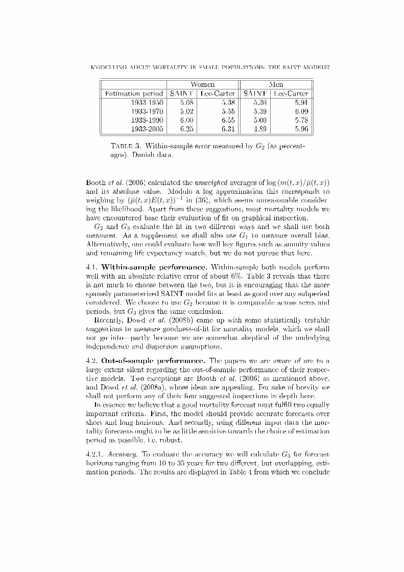
Table 3. Within-sample error measured by G2 (as percent-ages). Danish data.

Booth et al. (2006) calculated the unweighed averages of log (m(t, x)/µ(t, x))and its absolute value. Modulo a log approximation this corresponds toweighing by (µ(t, x)E(t, x))−1 in (36), which seems unreasonable consider-ing the likelihood. Apart from these suggestions, most mortality models wehave encountered base their evaluation of t on graphical inspection.

G2 and G3 evaluate the t in two dierent ways and we shall use bothmeasures. As a supplement we shall also use G1 to measure overall bias.Alternatively, one could evaluate how well key gures such as annuity valuesand remaining life expectancy match, but we do not pursue that here.

4.1. Within-sample performance. Within-sample both models performwell with an absolute relative error of about 6%. Table 3 reveals that thereis not much to choose between the two, but it is encouraging that the moresparsely parameterized SAINT model ts at least as good over any subperiodconsidered. We choose to use G2 because it is comparable across sexes andperiods, but G3 gives the same conclusion.

Recently, Dowd et al. (2008b) came up with some statistically testablesuggestions to measure goodness-of-t for mortality models, which we shallnot go intopartly because we are somewhat skeptical of the underlyingindependence and dispersion assumptions.

4.2. Out-of-sample performance. The papers we are aware of are to alarge extent silent regarding the out-of-sample performance of their respec-tive models. Two exceptions are Booth et al. (2006) as mentioned above,and Dowd et al. (2008a), whose ideas are appealing. For sake of brevity weshall not perform any of their four suggested inspections in depth here.

In essence we believe that a good mortality forecast must fulll two equallyimportant criteria. First, the model should provide accurate forecasts overshort and long horizons. And secondly, using dierent input data the mor-tality forecasts ought to be as little sensitive towards the choice of estimationperiod as possible, i.e. robust.

4.2.1. Accuracy. To evaluate the accuracy we will calculate G3 for forecasthorizons ranging from 10 to 35 years for two dierent, but overlapping, esti-mation periods. The results are displayed in Table 4 from which we conclude


Forecast period lengthEstimation period 10 15 20

SAINT LC SAINT LC SAINT LC1933-1950 0.69 0.43 0.93 0.69 1.34 1.311933-1970 1.48 2.32 2.39 4.27 3.50 6.96


SAINT LC SAINT LC SAINT LC1933-1950 2.43 2.81 4.26 5.34 6.44 8.581933-1970 4.82 9.70 6.22 13.0 7.27 15.7

Table 4. Out-of-sample error for dierent estimation peri-ods and dierent forecast periods measured by G3 (normal-ized by 106). Danish women.


SAINT LC SAINT LC SAINT LC1933-1950 -7.97 -1.64 -6.84 -0.62 -6.36 -0.331933-1970 -4.86 -3.28 -3.64 -2.35 -2.10 -1.21


SAINT LC SAINT LC SAINT LC1933-1950 -6.82 -1.04 -6.97 -1.51 -6.49 -1.391933-1970 +0.33 +0.80 +1.83 +1.93 +2.78 +2.53

Table 5. Out-of-sample error for dierent estimation peri-ods and dierent forecast periods measured by G1 (as per-centages). Danish women.

(albeit based on limited evidence and overlapping estimation periods) thatthe LC method predicts slightly more accurately over short forecast periods,whereas on long horizons the SAINT model's performance is superior. Fur-ther analysis has indicated that the tipping point lies between about ve and15 years' forecast.

At the cost of potentially even worse long run forecasts it has been sug-gested to improve the short run accuracy by calibrating the Lee-Carter modelto the latest observed death rates. This would likely reinforce the dierencebetween the two models.

Very short term forecasts (not shown) are quite accurate in both casesbecause of short term smoothness of data and the relatively dense parametriza-tion. All conclusions above apply to men as well.


For the same estimation and forecast periods we have calculated G1 as ameasure of bias. The results are shown in Table 5. Note that negative valuesimply upward bias of death rates, i.e. projected death rates are higher thanrealized death rates. For the short estimation period the SAINT model hasa higher bias than LC, while the bias of the two models is essentially thesame for the long estimation period.

Examining the contributions of G1 more thoroughly (numbers not shown)reveals that there is a seemingly systematical pattern in the errors of theSAINT model with most of the upward bias concentrated at ages below 40.Death rates for ages 4060 are in fact slightly downward biased, while deathrates for ages above 60 are essentially unbiased. Due to its structure the LCmodel suers no such systematic age bias.

Dowd et al. (2008a) point out that most mortality forecasts are upwardbiased. We nd the same, but of course this is not an intrinsic feature of themodels.4.2.2. Robustness. We will check robustness in two waysby examining thestability of forecasts towards the inclusion of additional years in each end ofthe data window. This serves two distinct purposes. Adding extra years inthe left side of the interval we examine the sensitivity towards the otherwisearbitrary choice of left end point of the input data. On the other hand addingyears in the right side allows analysis of the desired feature that forecastsdo not change substantially when the model is calibrated using new data.Of course these two tests are closely linked. For the sake of brevity wewill provide graphical indications only but obviously a version of the G3

measure, or something similar, should be considered as well to assess howclose forecasts based on dierent data are.

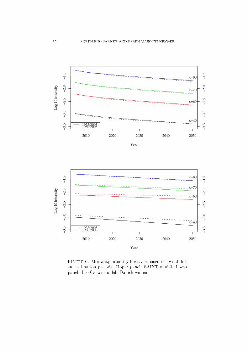
For the former analysis see Figure 6. This graphical inspection clearlyindicates that the SAINT model is more backward robust. The particularevidence is based on two scenarios only, but in fact the conclusion applies toother ages and periods and to Danish men as well.

Finally, we consider the stability towards including new data. This isessentially no dierent from the preceding analysis, and the conclusion isrepeated from above. Figure 7 compares mortality intensity forecasts attwo key ages and suggests that the SAINT model is slightly more forwardrobust. This conclusion is also representative across sexes, ages, and esti-mation periods.

We do not believe in the existence of an intrinsically optimal length forthe sample period. Hence, we do not investigate this. Instead we have faithin the underlying model and use as much data as possible whenever it isdeemed being of an acceptable quality.

As a closing remark we note that any full evaluation of the out-of-sampleperformance should take the entire tted and forecasted distribution intoaccount, cf. Dowd et al. (2008a). At rst glance our model seems to providereasonably wide distributions on both short and long horizons, thus nicelyaccompanying the reasonable forecasts. Presently we shall not, however,elaborate further on this.


2010 2020 2030 2040 2050

−3

.5−

3.0

−2

.5−

2.0

−1

.5

Year

Lo

g 1

0 i

nte

nsi

ty

x=40

x=60

x=70

x=80

1933:20051950:2005

−3

.5−

3.0

−2

.5−

2.0

−1

.5

2010 2020 2030 2040 2050

−3

.5−

3.0

−2

.5−

2.0

−1

.5

Year

Lo

g 1

0 i

nte

nsi

ty

x=40

x=60

x=70

x=80

1933:20051950:2005

−3

.5−

3.0

−2

.5−

2.0

−1

.5

Figure 6. Mortality intensity forecasts based on two dier-ent estimation periods. Upper panel: SAINT model. Lowerpanel: Lee-Carter model. Danish women.


2010 2020 2030 2040 2050

−2

.2−

1.8

−1

.4

Year

Lo

g 1

0 i

nte

nsi

ty

x=70

x=80

1933−19501933−19701933−19901933−2005

−2

.2−

1.8

−1

.4

2010 2020 2030 2040 2050

−2

.2−

1.8

−1

.4

Year

Lo

g 1

0 i

nte

nsi

ty

x=70

x=80

1933−19501933−19701933−19901933−2005

−2

.2−

1.8

−1

.4

Figure 7. Mortality intensity forecasts based on four dier-ent estimation periods. Upper panel: SAINT model. Lowerpanel: Lee-Carter model. Danish women.


5. Concluding remarksThe mainstream in mortality modeling builds on linear time series of un-

observed underlying random processes. This typically works very well whenthe population in question is suciently large that realised death rates aresmooth, in particular over relatively short forecast horizons. Over longerhorizons, and for small populations on the other hand the performance ofthese models is less convincing, and the estimates may be very sensitive to thechoice of input data. We therefore developed a two-step approachmodelingrst the mortality of a larger reference population, then the mortality spreadbetween the two populations.

We have left the choice of reference population a subjective one. Thereference population should be related to the population of interest as wehave to believe that the two populations share the same long term trend.Observing this, we recommend to choose it as large as possible for bestidentication of the trend. The analysis obviously depends on the choice ofreference population, but in this respect the choice of reference populationis no dierent from the choice of estimation window, or indeed the choice ofmodel.

In the presented model we have focused on forecasting a single population.However, the methodology can easily be extended to produce coherent, i.e.non-diverging, forecasts for a group of related populations by using the groupas reference population and treat each population as a subpopulation of thegroup. Similarly, we could consider men and women as subpopulations ofthe same population rather than estimate separate models for each gender asdone in the application. Using common and individual components to pro-duce coherent forecasts for related populations in the Lee-Carter frameworkhas been suggested by Li and Lee (2005).

We have used a two-stage estimation routine in which we rst estimate thetrend parameters and then estimate the spread parameters with the trendkept xed. This approach can be justied when the reference population issubstantially larger than the subpopulation, as in case of Danish and inter-national data. For applications in which the reference and subpopulationare of comparable size one might consider to estimate the trend and thespread jointly. It is straightforward to write down the likelihood function soin principle this is possible, but it is numerically involved due to the largenumber of parameters involved.

The trend component of the SAINT model imposes structure on howmortality can evolve over time and across ages. The parametric form providesinsight into the improvement patterns and it guarantees biologically plausibleforecasts. Compared to the Lee-Carter model the structure of the SAINTmodel lead to more precise long-term forecasts at the price of higher bias.The higher bias was primarily for young ages which is not surprising as thefocus of our modelling has been on old age mortality. The bias at young


ages could undoubtedly be reduced by more careful modelling of these agegroups if so desired.

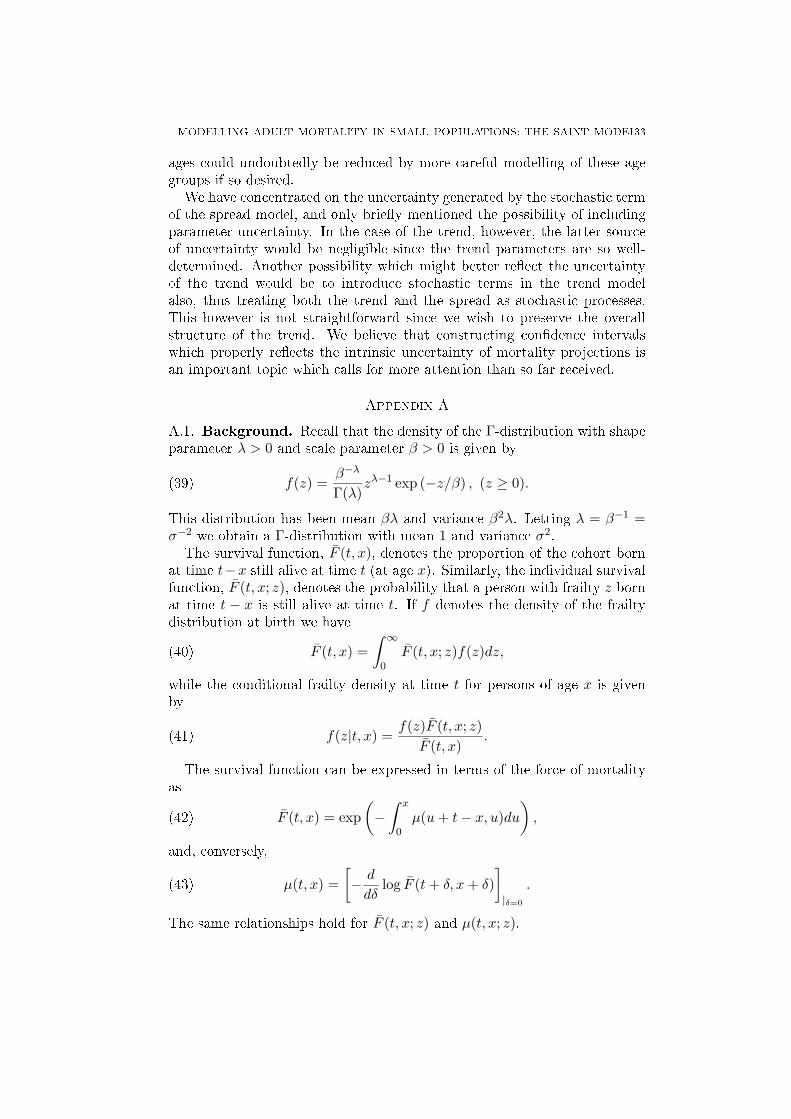
We have concentrated on the uncertainty generated by the stochastic termof the spread model, and only briey mentioned the possibility of includingparameter uncertainty. In the case of the trend, however, the latter sourceof uncertainty would be negligible since the trend parameters are so well-determined. Another possibility which might better reect the uncertaintyof the trend would be to introduce stochastic terms in the trend modelalso, thus treating both the trend and the spread as stochastic processes.This however is not straightforward since we wish to preserve the overallstructure of the trend. We believe that constructing condence intervalswhich properly reects the intrinsic uncertainty of mortality projections isan important topic which calls for more attention than so far received.

Appendix AA.1. Background. Recall that the density of the Γ-distribution with shapeparameter λ > 0 and scale parameter β > 0 is given by

(39) f(z) =β−λ

Γ(λ)zλ−1 exp (−z/β) , (z ≥ 0).

This distribution has been mean βλ and variance β2λ. Letting λ = β−1 =σ−2 we obtain a Γ-distribution with mean 1 and variance σ2.

The survival function, F (t, x), denotes the proportion of the cohort bornat time t−x still alive at time t (at age x). Similarly, the individual survivalfunction, F (t, x; z), denotes the probability that a person with frailty z bornat time t − x is still alive at time t. If f denotes the density of the frailtydistribution at birth we have

F (t, x) =∫ ∞

0F (t, x; z)f(z)dz,(40)

while the conditional frailty density at time t for persons of age x is givenby

(41) f(z|t, x) =f(z)F (t, x; z)

F (t, x).

The survival function can be expressed in terms of the force of mortalityas

(42) F (t, x) = exp(−

∫ x

0µ(u + t− x, u)du

),

and, conversely,

(43) µ(t, x) =[− d

dδlog F (t + δ, x + δ)

]

|δ=0

.

The same relationships hold for F (t, x; z) and µ(t, x; z).


A.2. Proofs.

Proof of Example 2.1. The rst equality in (10) follows from Proposition 2.1with µI

s(t, x) = α exp(βx) and γ(t) = γ, and the second equality follows fromProposition 2.2. ¤

Proof of Proposition 2.1. By (43), (40), (41) and (11) the population mor-tality satises

µ(t, x) =

[− ddδ F (t + δ, x + δ)

]|δ=0

F (t, x)

=

∫∞0 f(z)

[− ddδ F (t + δ, x + δ; z)

]|δ=0

dz

F (t, x)

=

∫∞0 f(z)F (t, x; z)µ(t, x; z)dz

F (t, x)

=∫ ∞

0f(z|t, x)

(zµI

s(t, x) + γ(t))dz

= E[Z|t, x]µIs(t, x) + γ(t).

¤

Proof of Proposition 2.2. Using (11), the individual survival function can bewritten

(44) F (t, x; z) = exp (−zI(t, x)−G(t, x)) ,

where I(t, x) =∫ x0 µI

s(u + t − x, u)du and G(t, x) =∫ x0 γ(t − x + u)du.

Inserting (44) in (40) with f given by (39) for λ = β−1 = σ−2 we get

F (t, x) =λλ

Γ(λ)

∫ ∞

0exp (−z [λ + I(t, x)]) zλ−1dz exp (−G(t, x))

=(

11 + σ2I(t, x)

)1/σ2

exp (−G(t, x)) .(45)

Finally, inserting (44) and (45) in (41) with f as above we obtain

f(z|t, x) =

(σ−2 + I(t, x)

)σ−2

Γ (σ−2)zσ−2−1e−z(σ−2+I(t,x)),

which we recognize as a Γ-density with λ = σ−2 and β−1 = σ−2+I(t, x). ¤

Proof of Proposition 2.3. First note that in the notation of Proposition 2.2we have (

∂

∂t+

∂

∂x

)I(t, x) = µI

s(t, x),


and thereby(∂

∂t+

∂

∂x

)log E[Z|t, x] = −

(∂

∂t+

∂

∂x

)log

(1 + σ2I(t, x)

)

= − σ2µIs(t, x)

1 + σ2I(t, x)

= −σ2µIs(t, x) E[Z|t, x]

= −σ2µs(t, x),

where the last equality follows from Proposition 2.1. Using E[Z|t− x, 0] = 1we then get

log E[Z|t, x] =∫ x

0

(∂

∂t+

∂

∂x

)log E[Z|t− x + u, u]du

= −σ2

∫ x

0µs(t− x + u, u)du.

¤Proof of Proposition 2.4. The equality in (24) follows from (17) and the spec-ication of µI

s. To show convergence we rst use Proposition 2.2 to write

(46) ∂ log E[Z|t, x]∂t

= −σ2 ∂∂tI(t, x)

1 + I(t, x),

where I(t, x) =∫ x0 K(t − x, y)dy. By (23) and dominated convergence we

have

I(t, x) =∫ x

0exp ((κ2 + g2y)t) K(−x, y)dy → 0 for t →∞,

since κ2 + g2y < 0 for all 0 ≤ y ≤ x by assumption. Similarly,∂

∂tI(t, x) =

∫ x

0exp ((κ2 + g2y)t) (κ2 + g2y)K(−x, y)dy → 0 for t →∞,

and we conclude that (46) also converges to zero. ¤Proof of Proposition 2.5. First case follows by applying l'Hôpital's rule to(22), second case is the Gamma-Makeham model, and third case is trivial.

¤


Appendix B

Country Period Male deaths Male exposure Female deaths Female exposureAustralia 1933-2004 3656554 298774817 3050957 304038560Austria 1947-2005 2362681 146948386 2544281 172938922Belgium 1933-2005 3959202 237960436 3655934 254715105Canada 1933-2005 5818067 501315204 4711059 510104624Denmark 1933-2005 1736235 118573885 1651576 124503893England & Wales 1933-2005 18790451 1155893702 18906239 1301265668Finland 1933-2005 1649803 105805700 1493332 118540078France 1933-2005 19554792 1197266420 18601741 1332188094Iceland 1933-2005 50595 4531626 46223 4597037Italy 1933-2004 17840263 1231244196 16616547 1360392086Japan 1947-2005 22944373 2115001379 19852118 2274227259Netherlands 1933-2005 3785909 304422103 3442716 316942482Norway 1933-2005 1326283 94013584 1240955 98579501Portugal 1940-2005 2859456 189334582 2769074 216359565Spain 1933-2005 10815395 785643871 9940870 862709017Sweden 1933-2005 2969115 202088902 2792398 209883920Switzerland 1933-2005 1949244 145118601 1888688 159060151USA 1933-2005 67513137 4756496475 58192508 5127612213West Germany 1956-2005 16193960 1081937335 17307798 1227848814

Table 6. Summary of deaths and exposures for ages 20-100over the period 1933-2005 for the countries included in theinternational data set. Source: The Human Mortality Data-base (www.mortality.org).

REFERENCES 37

ReferencesAndreev, K. F. (2002). Evolution of the Danish Population from 1835 to

2000. Monographs on Population Aging, 9. Odense University Press.Barbi, E. (2003). Assessing the rate of ageing of the human population.

Working Paper. Max Planck Institute for Demographic Research.Bongaarts, J. (2005). Long-range trends in adult mortality: Models and

projection methods. Demography 42, 2349.Booth, H., Hyndman, R. J., Tickie, L., and de Jong, P. (2006). Lee-Carter

mortality forecasting: A multi-country comparison of variants and ex-tensions. Demographic Research 15, 289310.

Booth, H., Maindonald, J., and Smith, L. (2002). Applying Lee-Carter underconditions of varying mortality decline. Population Studies 56, 325336.

Brockwell, P. J. and Davis, R. A. (1991). Time Series: Theory and Methods,Second Edition. Springer-Verlag, New York.

Brouhns, N., Denuit, M., and Vermunt, J. K. (2002). A Poisson log-bilinearregression approach to the construction of projected lifetables. Insur-ance: Mathematics and Economics 31, 373393.

Cairns, A. J., Blake, D., and Dowd, K. (2006). A two-factor model for sto-chastic mortality with parameter uncertainty: Theory and calibration.Journal of Risk and Insurance 73, 687718.

Cairns, A. J. G. (2000). A discussion of parameter and model uncertaintyin insurance. Insurance: Mathematics and Economics 27, 313330.

Currie, I. D., Durban, M., and Eilers, P. H. C. (2004). Smoothing andforecasting mortality rates. Statistical Modelling 4, 279298.

de Jong, P. and Tickle, L. (2006). Extending Lee-Carter mortality forecast-ing. Mathematical Population Studies 13, 118.

Dowd, K., Cairns, A. J. G., Blake, D., Coughlan, G. D., Epstein, D., andKhalaf-Allah, M. (2008a). Backtesting stochastic mortality models: Anex-post evaluation of multi-period-ahead density forecasts. Pensions In-stitute Discussion paper PI-0803.

Dowd, K., Cairns, A. J. G., Blake, D., Coughlan, G. D., Epstein, D., andKhalaf-Allah, M. (2008b). Evaluating the goodness of t of stochasticmortality models. Pensions Institute Discussion paper PI-0802.

Efron, B. and Tibshirani, R. J. (1993). An Introduction to the Bootstrap.Chapman & Hall, New York.

Gavrilov, L. A. and Gavrilova, N. S. (1991). The Biology of Life Span: AQuantitative Approach, ed. V. P. Skulachev. Harwood Academic Pub-lishers, Chur.

Jarner, S. F., Kryger, E. M., and Dengsøe, C. (2008). The evolution of deathrates and life expectancy in Denmark. Scandinavian Actuarial Journal108, 147173.

Koissi, M.-C., Shapiro, A. F., and Högnäs, G. (2006). Evaluating and ex-tending the Lee-Carter model for mortality forecasting: Bootstrap con-dence intervals. Insurance: Mathematics and Economics 38, 120.

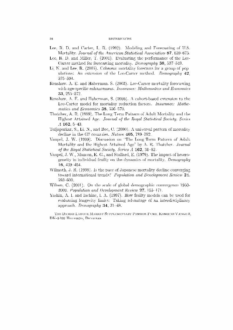
38 REFERENCES

Lee, R. D. and Carter, L. R. (1992). Modeling and Forecasting of U.S.Mortality. Journal of the American Statistical Association 87, 659675.

Lee, R. D. and Miller, T. (2001). Evaluating the performance of the Lee-Carter method for forecasting mortality. Demography 38, 537549.

Li, N. and Lee, R. (2005). Coherent mortality forecasts for a group of pop-ulations: An extension of the Lee-Carter method. Demography 42,575594.

Renshaw, A. E. and Haberman, S. (2003). Lee-Carter mortality forecastingwith age-specic enhancement. Insurance: Mathematics and Economics33, 255272.

Renshaw, A. E. and Haberman, S. (2006). A cohort-based extension to theLee-Carter model for mortality reduction factors. Insurance: Mathe-matics and Economics 38, 556570.

Thatcher, A. R. (1999). The Long-Term Pattern of Adult Mortality and theHighest Attained Age. Journal of the Royal Statistical Society. SeriesA 162, 543.

Tuljapurkar, S., Li, N., and Boe, C. (2000). A universal pattern of mortalitydecline in the G7 countries. Nature 405, 789792.

Vaupel, J. W. (1999). Discussion on The Long-Term Pattern of AdultMortality and the Highest Attained Age by A. R. Thatcher. Journalof the Royal Statistical Society. Series A 162, 3132.

Vaupel, J. W., Manton, K. G., and Stallard, E. (1979). The impact of hetero-geneity in individual frailty on the dynamics of mortality. Demography16, 439454.

Wilmoth, J. R. (1998). Is the pace of Japanese mortality decline convergingtoward international trends? Population and Development Review 24,593600.

Wilson, C. (2001). On the scale of global demographic convergence 1950-2000. Population and Development Review 27, 155171.

Yashin, A. I. and Iachine, I. A. (1997). How frailty models can be used forevaluating longevity limits: Taking advantage of an interdisciplinaryapproach. Demography 34, 3148.

The Danish Labour Market Supplementary Pension Fund, Kongens Vænge 8,DK-3400 Hillerød, Denmark

modelling adult mortality in small - demografi · modelling adult mortality in small populations:...

Documents