modélisation et contrôle d’un système de convoyage...
TRANSCRIPT
Modélisation et contrôle d’un système de
convoyage automatisé.
Relatório submetido à Universidade Federal de Santa Catarina
como requisito para a aprovação da disciplina:
DAS 5511: Projeto de Fim de Curso
Matheus Silva Dias
Florianópolis, Janeiro de 2016

Modélisation et contrôle d’un système de convoyage
automatisé
Matheus Silva Dias
Esta monografia foi julgada no contexto da disciplina
DAS 5511: Projeto de Fim de Curso
e aprovada na sua forma final pelo
Curso de Engenharia de Controle e Automação
Prof. Dr. José Eduardo Ribeiro Cury

Banca Examinadora:
Prof. Laurent Hardouin, Dr.Orientador na Empresa
Prof. José Eduardo Ribeiro Cury, Dr.Orientador no Curso
Prof.Júlio Elias Normey Rico, Dr.
Prof.Hector Bessa Silveira, Dr.
Prof. xxxxxxx, Avaliador
aluno1, Debatedor
aluno2, Debatedor

Acknowledgements


Resumo

Remerciements


Abstract
In this document will be presented a control strategy for Max-Plus-Linear (MPL) systems, aclass of discrete-event systems widely used in synchronization and scheduling applications,such as: production systems (flexible workshops, assembly lines), communication networks(computer networks) and for transport systems (road, rail and air traffic). This document presentsan observer-based controller with a real system application, located at ISTIA -École d’Ingénieursde l’Université d’Angers.
Keywords: Discrete Event Systems, (Max,+) Linear Systems, Control Theory.


Resumo
Neste documento será apresentada uma estratégia de controle para sistemas Max-Plus lineares,uma classe de sistemas à eventos discretos largamente utilizada em sincronização e aplicaçõesde escalonamento, tais como: sistemas de produção (oficinas flexíveis, linhas de montagem),redes de comunicação (redes de computadores) e sistemas de transporte (rodoviário, ferroviárioe aéreo). Este documento apresenta um controlador baseado em observador, com um sistemareal de aplicação, localizado no ISTIA - École d’Ingénieurs de l’Université d’Angers.
Palavras-chave: Sistemas à eventos discretos, Sistemas (Max,+) lineares, Teoria de controle.

Résumé
Dans ce document sera présenté une stratégie de contrôle pour les systèmes linéaires Max-Plus, une classe de systèmes à événements discrets largement utilisés pour des applications desynchronisation et d’ordonnancement, tels que les systèmes de production (ateliers flexibles,lignes d’assemblage), les réseaux de communication (réseaux informatiques) et des systèmes detransport (routier, ferroviaire et aérien). Ce document présente un contrôleur basé en observateuravec un système d’application réelle, située dans ISTIA - Ecole d’Ingénieurs de l’Universitéd’Angers.
Mots-clés: Systèmes à evénements discrets, Systèmes (Max,+) linéaires, Théorie de contrôle.


List of Figures
Figure 1 – Hasse diagram of an ordered set ({a, b, c, d},�) . . . . . . . . . . . . . . . 22Figure 2 – Hasse diagram of the lattice (P(E),[,\) with E = {a, b, c}. . . . . . . . . 24Figure 3 – Hasse diagram of semi-lattice ({1, 2, 3, 4, 5, 6},�
div
). . . . . . . . . . . . . 25Figure 4 – F : � and E: • with F = E\{a _ b, a ^ b} . . . . . . . . . . . . . . . . . . 26Figure 5 – The graph corresponding to matrix of size 2⇥ 2 . . . . . . . . . . . . . . . 41Figure 6 – A Timed Event Graph which can represent a manufacturing system with
three machines labeled M1
to M3
. . . . . . . . . . . . . . . . . . . . . . . . 45Figure 7 – Example an assembly line (event extension). . . . . . . . . . . . . . . . . . 47Figure 8 – Assembly line with temporization lower than or equal to 1 (temporal extension.) 50Figure 9 – Graphical representation of series s = p� qr⇤ = e� �� � �4�3 � (�5�5 �
�7�6)(�4�3)⇤. . . . . . . . . . . . . . . . . . . . . . . . . . . . . . . . . . 64Figure 10 – Model matching : state feedback architecture. . . . . . . . . . . . . . . . . 65Figure 11 – Observer architecture . . . . . . . . . . . . . . . . . . . . . . . . . . . . . 66Figure 12 – Control architecture using the estimated state . . . . . . . . . . . . . . . . . 67Figure 13 – The Observer-based Controller . . . . . . . . . . . . . . . . . . . . . . . . 68Figure 14 – Photo of the system in the Laboratoire Angevin de Recherche en Ingénierie
des Systèmes (LARIS) at the Université d’Angers. . . . . . . . . . . . . . . 69Figure 15 – Three pallets in a line, approaching a button . . . . . . . . . . . . . . . . . 70Figure 16 – Schematic picture of the transportation system . . . . . . . . . . . . . . . . 71Figure 17 – TEG for B1-B2 . . . . . . . . . . . . . . . . . . . . . . . . . . . . . . . . 73Figure 18 – Full TEG . . . . . . . . . . . . . . . . . . . . . . . . . . . . . . . . . . . . 79Figure 19 – Development environment - CodeBlocks . . . . . . . . . . . . . . . . . . . 81


Contents
1 INTRODUCTION . . . . . . . . . . . . . . . . . . . . . . . . . . . . . 191.1 Motivation . . . . . . . . . . . . . . . . . . . . . . . . . . . . . . . . . . 191.2 LARIS . . . . . . . . . . . . . . . . . . . . . . . . . . . . . . . . . . . . . 191.3 Objectives . . . . . . . . . . . . . . . . . . . . . . . . . . . . . . . . . . 191.4 Organization . . . . . . . . . . . . . . . . . . . . . . . . . . . . . . . . . 19
2 ALGEBRAIC PRELIMINARIES . . . . . . . . . . . . . . . . . . . . . 212.1 Lattices and order sets . . . . . . . . . . . . . . . . . . . . . . . . . . 212.2 Idempotent semiring . . . . . . . . . . . . . . . . . . . . . . . . . . . . 252.3 Mappings defined over idempotent semirings . . . . . . . . . . . . 282.4 Fixed points of monotone mappings . . . . . . . . . . . . . . . . . . 312.4.1 Properties of the Kleene star operator . . . . . . . . . . . . . . . . . . . 322.5 Residuation theory . . . . . . . . . . . . . . . . . . . . . . . . . . . . . 332.6 Semiring Z
max
. . . . . . . . . . . . . . . . . . . . . . . . . . . . . . . . 392.6.1 Matrices sum . . . . . . . . . . . . . . . . . . . . . . . . . . . . . . . . . 392.6.2 Matrices product . . . . . . . . . . . . . . . . . . . . . . . . . . . . . . . 392.7 Equation x = ax� b . . . . . . . . . . . . . . . . . . . . . . . . . . . . . 402.7.1 Equation ax � b . . . . . . . . . . . . . . . . . . . . . . . . . . . . . . . 412.7.2 Spectral theory of matrices . . . . . . . . . . . . . . . . . . . . . . . . . 42
3 SYSTEM MODELLING AND CONTROL THEORY . . . . . . . . . . 433.1 Model for systems subject to synchronization and delay . . . . . 433.1.1 Daters equations, the event point of view . . . . . . . . . . . . . . . . . 433.1.2 Counters Equations, the time point of view . . . . . . . . . . . . . . . . 483.1.3 Semiring of formal series . . . . . . . . . . . . . . . . . . . . . . . . . . 513.1.3.1 Semiring Z
max
[[�]] . . . . . . . . . . . . . . . . . . . . . . . . . . . . . . . . 52
3.1.3.2 Monotonic Trajectories . . . . . . . . . . . . . . . . . . . . . . . . . . . . . 53
3.1.3.3 Semiring Zmin
[[�]] . . . . . . . . . . . . . . . . . . . . . . . . . . . . . . . . 53
3.1.3.4 Monotonic trajectories . . . . . . . . . . . . . . . . . . . . . . . . . . . . . . 54
3.1.4 Two-dimensionnal description, semiring Max
in
[[�, �]] . . . . . . . . . . . . 553.2 Control Theory . . . . . . . . . . . . . . . . . . . . . . . . . . . . . . . 563.2.1 State feedback controller synthesis . . . . . . . . . . . . . . . . . . . . 563.2.2 Observer synthesis . . . . . . . . . . . . . . . . . . . . . . . . . . . . . 573.2.2.1 Application : Control with observer . . . . . . . . . . . . . . . . . . . . . . . . 59
3.2.2.2 Illustration . . . . . . . . . . . . . . . . . . . . . . . . . . . . . . . . . . . . 60
3.2.3 Modified Observer-based controller . . . . . . . . . . . . . . . . . . . . 61

4 AUTOMATED CONVEYOR SYSTEM . . . . . . . . . . . . . . . . . . 694.1 System Description . . . . . . . . . . . . . . . . . . . . . . . . . . . . 724.2 System Modelling . . . . . . . . . . . . . . . . . . . . . . . . . . . . . . 744.3 Control System . . . . . . . . . . . . . . . . . . . . . . . . . . . . . . . 764.3.1 Time domain representation of u . . . . . . . . . . . . . . . . . . . . . . 76
5 IMPLEMENTATION . . . . . . . . . . . . . . . . . . . . . . . . . . . . 815.1 Code . . . . . . . . . . . . . . . . . . . . . . . . . . . . . . . . . . . . . . 81
6 RESULTS . . . . . . . . . . . . . . . . . . . . . . . . . . . . . . . . . 896.1 Simulation Results . . . . . . . . . . . . . . . . . . . . . . . . . . . . . 906.2 Simulation Analysis . . . . . . . . . . . . . . . . . . . . . . . . . . . . 91
7 CONCLUSION . . . . . . . . . . . . . . . . . . . . . . . . . . . . . . 93
BIBLIOGRAPHY . . . . . . . . . . . . . . . . . . . . . . . . . . . . . 95
APPENDIX 97
APPENDIX A – TRANSFER FUNCTION AND CONTROLLERS . . 99
19
1 Introduction
1.1 Motivation
1.2 LARIS
The Angevin Laboratory for Research in Systems Engineering is a host team of theUniversity of Angers, consisting of 3 interconnected teams:
• Dynamical Systems and Optimisation (SDP);
• Information, Signal, Image and Life Sciences (ISISV);
• Operational Safety and assistance in Decision (SFD)
1.3 Objectives
The specific objectives of this work are:
• To represent the automated conveyor system, located at ISTIA, using (max,+ algebra);
• To use and test the performance of an Observer-based Controller for (Max,+) LinearSystems.
1.4 Organization
This document is organized as follows:
• Chapter 1 - Introduction;
• Chapters 2 and 3 - Algebraic Preliminaries/System Modelling and Control Theory: Chap-ters 3 and 4 were granted by Prof. Dr. Laurent Hardouin, the following chapters are presentin his handout [1]. These chapters present the main algebraic tools useful in the sequence.In the last section of chapter 3 I will introduce the Modified Observer-based Controller,my first participation during the work in LARIS.
• Chapter 4 - Automated conveyor system: A TEG model for the automated conveyor systemis proposed in Dr. Vinícius Mariano’s thesis [21] and used to construct a model with theTwo-dimentinal description, the semiring Max
in
[[�, �]].
20 Chapter 1. Introduction
• Chapter 5 - Implementation;
• Chapter 6 - Simulation results;
• Chapter 7 - Conclusion.

21
2 Algebraic Preliminaries
This chapter presents the main algebraic tools useful in the sequence. It is not anexhaustive presentation but a survey of definitions, theorems necessary to prove the resultsintroduced in the next chapters. In a first reading, the engineer could skip this chapter andpick inside the useful results during the reading of the chapters dedicated to the applications.The theory of (max,+) linear systems is partially based on the lattice theory and the mannerto invert mappings defined over ordered sets, the following references were also source ofinspiration [2], [3], [4].The chapter is organized as follows :
• Elementary definitions about lattice theory basic facts are recalled in a first part, they willbe useful to understand the proof of the results given in the sequel. There are usual notionsfor computer scientists but not necessary for engineers involved in the automatic controltheory.
• The algebraic structure considered is the idempotent semiring.
2.1 Lattices and order sets
For very detailed presentation about Lattices, the reader is invited to consult the followingreferences [2–4]. Some recalls are also available in chapter 4 of [5].
Definition 1 (Order relation, ordered set). An order relation is a binary relation which is reflexive,transitive and anti-symmetric : Let E be a set and a binary relation on this set denoted �, thisrelation is an order relation if and only if for all x, y, and z elements of E :
• x � x (reflexivity)
• (x � y et y � x) ) x = y (anti-symmetry)
• (x � y et y � z) ) x � z (transitivity)
An ordered set is a set (E,�) endowed with an order relation.
Let x, y 2 (E,�), x and y are said comparable (according to the order relation �) if
x � y or y � x.
Conversely, two elements x, y 2 (E,�) such that x 6� y and y 6� x, are said to be notcomparable.

22 Chapter 2. Algebraic Preliminaries
If 8x, y 2 (E,�), x and y are comparable then the order is said to be a total order, and(E,�) is said to be totally ordered. Conversely, if it exists a couple x, y 2 (E,�), such thatx 6= y and x and y are not comparable, then the order is said to be partial and (E,�) is said tobe partially ordered.
Remark 2. In ambiguous situation, the order relation of set E will be denoted �E
.
All subset F of an ordered set (E,�) is an ordered set with an order relation restrictedto the elements of F , and denoted �
F
. This order is simply defined as
x, y 2 F ⇢ E, x � y () x �F
y.
Remark 3. If (E,�) is partially ordered, a subset F ⇢ E can be such that all the elements ofF be not comparable.
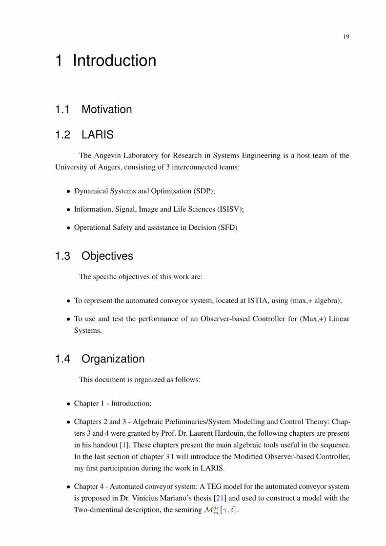
A finite ordered set (E,�) can be represented by a graph called Hasse diagram. Eachelement of E is depicted by a vertex(•). An edge lying two vertices of the diagram means thatthe elements depicted by these vertices are comparable. By convention, the order is chosen toincrease from the bottom to the top of the diagram.
�6
t��� t@@@tt
a b
c
d
a � c, b � c, c � d
a � d, b � d (by transitivity of the order �)
Figure 1 – Hasse diagram of an ordered set ({a, b, c, d},�)
On figure 1, set E = {a, b, c, d} is partially ordered according to order relation � despitedby the diagram. Subset F = {a, b} ⇢ E is an ordered set by considering the restriction of � toF , and all its elements are not comparable.
Remark 4. A totally ordered set is also called a chain according to its Hasse diagram whichlooks like a chain.
Example 5 (Ordered sets).
• (R,), (Z,), (N,), (Q,) where is the natural order, are totally ordered sets.
• Let E be a set, and P(E) be the set of all the subset of E. The latest is an ordered set bythe inclusion relation. This ordered set is denoted (P(E),⇢) and it is a partially orderedset. Indeed, two disjoints subsets of E are not comparable according to the order ⇢.
2.1. Lattices and order sets 23
• Let (E,�E
) be an ordered set. The set of matrices with entries in E, namely En⇥m isan ordered set. Even if �
E
is total on E, the order obtained on En⇥m is only partial.Furthermore,
A �E
n⇥m B , aij
�E
bij
8(i, j),
where A and B are matrices of En⇥m.
• Let (E,�E
) and (F,�)
F be ordered sets. The set Map(E,F ) of all mappings from E toF can be ordered by defining the following order relation
f �Map(E,F )
g , f(x) �F
g(x)8x 2 E.
Definition 6 (Upper bound, lower bound). Let (E,�) be an ordered set and F ⇢ E a non emptysubset of E. An element z 2 E satisfying 8x 2 F, z ⌫ x (resp. z � x) is called upper bound(resp. lower bound) of set F .
Remark 7 (Bounds of a set). When it exists, the least upper bound (lub) of set F ⇢ E is denotedW
F . As well, when it exists, the greatest lower bound (glb) of F is denotedV
F . When thesebounds are defined, all the upper bounds of F are greater than or equal to
WF and all lower
bounds of F are lower than or equal toV
F .
Definition 8. Let E be an ordered set.
• if x _ y exists 8x, y 2 E then E is a sup-semi-lattice.
• ifW
F exists 8F ⇢ E then F is a complete sup-semi-lattice.
Definition 9. Let E be an ordered set.
• if x ^ y exists 8x, y 2 E then E is an inf-semi-lattice.
• ifV
F exists 8F ⇢ E then F is a complete inf-semi-lattice.
Definition 10. Let E be an ordered set.
• if x _ y and x ^ y exist 8x, y 2 E then E is a lattice.
• ifW
F andV
F exist 8F ⇢ E then F is a complete lattice.
Lemma 11. Let E be a lattice and a, b 2 E, then the following equivalences hold :
a � b , a _ b = b , a ^ b = a.
Theorem 12. Let E be a lattice, 8a, b, c 2 E, _ and ^ the following properties hold:
• associativity : a _ (b _ c) = (a _ b) _ c and a ^ (b ^ c) = (a ^ b) ^ c,• commutativity : a _ b = b _ a and a ^ b = b ^ a,• idempotency : a _ a = a and a ^ a = a,• absorption : a _ (a ^ b) = a and a ^ (a _ b) = a.
24 Chapter 2. Algebraic Preliminaries
Remark 13 (Duality principle). The inverse of an order relation � is an order relation denoted�⇤. Consequently, if (E,�) is a sup-semi-lattice, (E,�⇤
) is an inf-semi-lattice, and vice versa.Furthermore, a relation involving �, _ and ^ is still valid by replacing � by �⇤ and by permuting_ and ^. This is called the duality principle.
Example 14. The ordered set depicted by the Hasse diagram of figure 1 is a sup-semi-lattice.But it is not an inf-semi-lattice since a ^ b does not exist.
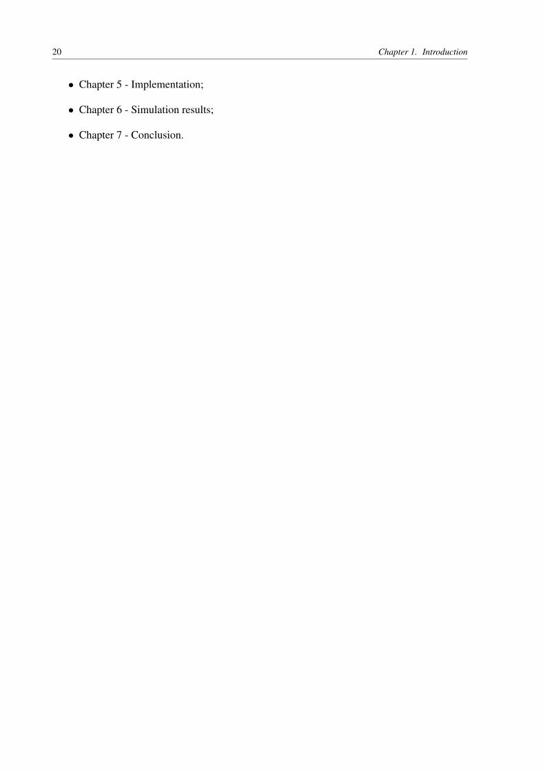
Example 15. Let E = {a, b, c} and P(E) the set of subset of E. Then (P(E),[,\) has a latticestructure if the empty set is considered as the lowest subset of E. The Hasse diagram of thislattice is given in figure 2.
s ?s{a} s{b} s{c}
s{a, b} s{a, c} s{b, c}
sE = {a, b, c}
����
@@
@@�
���
@@
@@
����
@@
@@
����
����
@@
@@
Figure 2 – Hasse diagram of the lattice (P(E),[,\) with E = {a, b, c}.
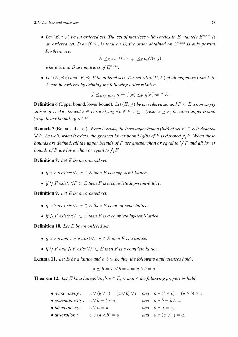
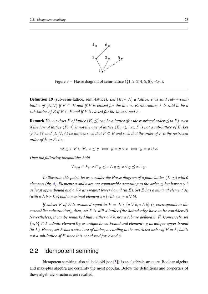
Example 16. Let (N⇤,�div
) be the set of positive integers, where the order on N⇤ is defined as
a �div
b () a divides b, (2.1)
is a lattice. The lattice laws of (N⇤,�div
) are defined as a_b = ppcm(a, b) and a^b = pgcd(a, b).In figure 3 the Hasse diagram corresponding to the set E = {1, 2, 3, 4, 5, 6} according to theorder relation �
div
is given. Set (E,�div
) ⇢ N⇤ is an inf-semi-lattice.
Example 17. By adding element +1 to Z, set (Z [ {+1},) is _-complete totally orderedset. On the other hand, (Q [ {+1},) is a totally ordered set which is not _-complete and not^-complete. For instance, subset {x 2 Q|x
p2} of Q has no least upper bound (lub) in Q.
Definition 18 (Distributive lattice). Lattice (E,_,^) is distributive if laws _ and ^ distributeon each other, i.e.
a _ (b ^ c) = (a _ b) ^ (a _ c), (2.2)
a ^ (b _ c) = (a ^ b) _ (a ^ c). (2.3)
2.2. Idempotent semiring 25
s1
s2 s3 s5
s4 s6
AA
AA
����
⌘⌘⌘⌘
⌘⌘����
Figure 3 – Hasse diagram of semi-lattice ({1, 2, 3, 4, 5, 6},�div
).
Definition 19 (sub-semi-lattice, semi-lattice). Let (E,_,^) a lattice. F is said sub-_-semi-lattice of (E,_) if F ⇢ E and if F is closed for the law _. Furthermore, F is said to be asub-lattice of E if F ⇢ E and if F is closed for the laws _ and ^.
Remark 20. A subset F of lattice (E,�) can be a lattice (for the restricted order � to F ), evenif the law of lattice (F,�) is not the one of lattice (E,�), i.e., F is not a sub-lattice of E. Let(F,[,\) and (E,_,^) be lattices such that F ⇢ E and such that the order of F is the restrictedorder of E to F , i.e.
8x, y 2 F ⇢ E, x � y () y = y _ x () y = y [ x.
Then the following inequalities hold
8x, y 2 F, x \ y � x ^ y � x _ y � x [ y.
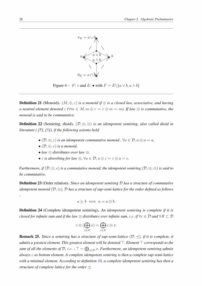
To illustrate this point, let us consider the Hasse diagram of a finite lattice (E,�) with 6elements (fig. 4). Elements a and b are not comparable according to the order � but have a _ b
as least upper bound and a ^ b as greatest lower bound (in E). Set E has a minimal element 0E
(with a ^ b � 0
E
) and a maximal element ⇡E
(with ⇡E
� a _ b).
If subset F of E is assumed equal to F = E \ {a _ b, a ^ b} (\ corresponds to theensemblist substraction), then, set F is still a lattice (the dotted edge have to be considered).Nevertheless, it can be remarked that neither a _ b, nor a ^ b are defined in F . Conversely, set{a, b} ⇢ F admits element 0
E
as unique lower bound and element ⇡E
as unique upper bound(in F ). Hence, set F has a structure of lattice, according to the restricted order of E to F , but isnot a sub-lattice of E since it is not closed for _ and ^.
2.2 Idempotent semiring
Idempotent semiring, also called dioid (see [5]), is an algebraic structure. Boolean algebraand max-plus algebra are certainly the most popular. Below the definitions and properties ofthese algebraic structures are recalled.
26 Chapter 2. Algebraic Preliminaries
sfsssf
sfa sfba ^ ba _ b
0
E
= a \ b
⇡E
= a [ b
HHHH����
����HHHH
JJ
JJ
JJ
⌦⌦
⌦⌦
⌦⌦⌦⌦
⌦⌦
⌦⌦
JJ
JJ
JJ
Figure 4 – F : � and E: • with F = E\{a _ b, a ^ b}
Definition 21 (Monoid). (M,�, ") is a monoid if � is a closed law, associative, and havinga neutral element denoted " (8m 2 M,m � " = " � m = m). If law � is commutative, themonoid is said to be commutative.
Definition 22 (Semiring, dioid). (D,�,⌦) is an idempotent semiring, also called dioid inliterature ( [?], [5]), if the following axioms hold
• (D,�, ") is an idempotent commutative monoid , 8a 2 D, a� a = a,• (D,⌦, e) is a monoid,• law ⌦ distributes over law �,• " is absorbing for law ⌦, 8a 2 D, a⌦ " = "⌦ a = ".
Furthermore, if (D,⌦, e) is a commutative monoid, the idempotent semiring (D,�,⌦) is said tobe commutative.
Definition 23 (Order relation). Since an idempotent semiring D has a structure of commutativeidempotent monoid (D,�), D has a structure of sup-semi-lattice for the order defined as follows:
a ⌫ b () a = a� b.
Definition 24 (Complete idempotent semiring). An idempotent semiring is complete if it isclosed for infinite sum and if the law ⌦ distributes over infinite sum, i.e. if 8c 2 D and 8X ⇢ D
c⌦ (
M
x2X
x) =M
x2X
c⌦ x.
Remark 25. Since a semiring has a structure of sup-semi-lattice (D,�), if it is complete, itadmits a greatest element. This greatest element will be denoted >. Element > corresponds to thesum of all the elements of D, i.e. : > =
Lx2D x. Furthermore, an idempotent semiring admits
always " as bottom element. A complete idempotent semiring is then a complete sup-semi-latticewith a minimal element. According to definition 10, a complete idempotent semiring has then astructure of complete lattice for the order �.

2.2. Idempotent semiring 27
Definition 26. If D is a complete idempotent semiring, then the law ^ defined as
a ^ b =M
x�a,x�b
x,
is associative, commutative and idempotent, furthermore (D,�,^) is a complete lattice and thefollowing equivalences hold
a = a� b , a ⌫ b , b = a ^ b. (2.4)
Remark 27. According to definition 24, laws �, ⌦, ^ are order preserving, i.e, 8a, b, c 2 D thefollowing implication hold :
a � b ) a⌦ c � b⌦ c,
a � b ) a� c � b� c,
a � b ) a ^ c � b ^ c.
Remark 28. Relation (2.4) looks like operators � and ^ play a symmetric role. That is truefrom the lattice point of view since operator � corresponds to _ and thanks to the dualityprinciple. But that is false if we consider the second operator of the semiring ⌦, since there is nodistributivity of ^ over ⌦ in a general manner. Nevertheless, the product being order preserving(see Remark 27, the following sub distributivity holds :
c⌦ (a ^ b) � (c⌦ a) ^ (c⌦ b) 8a, b, c 2 D.
Example 29 ((max,plus) algebra). Zmax
= (Z[{�1,+1},max,+) is a complete idempotentsemiring such that a� b = max(a, b), a⌦ b = a+ b, a ^ b = min(a, b) with " = �1, e = 0,and > = +1. The order � is total and corresponds to the natural order . By extension Zn⇥m
max
is a semiring of matrices with entries in Zmax
. Matrix " 2 Zn⇥m
max
will be such that all its entriesare equal to " 2 Z
max
, matrix " 2 Zn⇥n
max
will be such that all the entries are equal to " 2 Zmax
except the diagonal entries which are equal to e 2 Zmax
. This semiring will be of main interestin the sequel and section 2.6 will be devoted to present some of its properties.
Example 30 ((min,plus) algebra). Zmin
= (Z [ {�1,+1},min,+) is a complete idempotentsemiring such that a� b = min(a, b), a⌦ b = a+ b, a ^ b = max(a, b) with " = +1, e = 0,and > = �1. The order � is total and corresponds to the inverse of the natural order (i.e.,2 � 1). Semiring of matrices Zn⇥m
min
is a semiring of matrices with the entries in Zmin
.
Example 31 ((max,min) algebra). The set (Z [ {�1,+1},max,min) is a complete idempo-tent semiring such that a � b = max(a, b), a ⌦ b = min(a, b) with " = �1, e = +1, and> = +1, in this semiring a ^ b = min(a, b).
Definition 32 (Distributive semiring). A semiring D is distributive if it is complete and if thelattice (D,�,^) is distributive (cf. Definition 18).
28 Chapter 2. Algebraic Preliminaries
Remark 33. Laws � and ^ are order preserving (see property 27), hence if the semiring is notdistributive, the following inequalities hold :
a� (b ^ c) � (a� b) ^ (a� c),
a ^ (b� c) ⌫ (a ^ b)� (a ^ c).
Definition 34 (Subsemiring). Let (D,�,⌦) be a semiring and C ⇢ D. (C,�,⌦) is a subsemir-ing of D if ", e 2 C and if C is closed for laws � and ⌦. A subsemiring is complete if it is closedfor infinite sums too.
2.3 Mappings defined over idempotent semirings
Definition 35 (Continuity). A mapping ⇧ defined from a complete idempotent semiring D to acomplete idempotent semiring C is lower semi-continuous (denoted l.s.c.), respectively uppersemi-continuous (denoted u.s.c), if for all finite or infinite set X of D,
⇧(
M
x2X
x) =M
x2X
⇧(x),
respectively,⇧(
^
x2X
x) =^
x2X
⇧(x).
Mapping ⇧ is continuous if it is both l.s.c. and u.s.c..
Definition 36 (Isotone, antitone, monotone). Let ⇧ : D ! C be a mapping, with D and C twoidempotent semirings :
• mapping ⇧ is isotone if it is order preserving, i.e., 8x, x0 2 D x � x0 ) ⇧(x) � ⇧(x0),
• mapping ⇧ is antitone if it inverts the order, i.e., 8x, x0 2 D x � x0 ) ⇧(x) ⌫ ⇧(x0),
• mapping ⇧ is monotone, i.e., ⇧ isotone or ⇧ antitone.
Remark 37. The composition of monotone functions is a monotone function and it can easily bechecked that :
• The composition of isotone functions is an isotone function.
• The composition of two antitone functions is isotone.
• The composition of an isotone function with an antitone function is antitone.
Theorem 38. Let ⇧ : D ! C be a mapping with D and C two semirings :
2.3. Mappings defined over idempotent semirings 29
1. if ⇧ is l.s.c then it is isotone.
2. if ⇧ is u.s.c then it is isotone.
Remark 39. If ⇧ : D ! C is an isotone mapping, the following inequality holds
⇧(x� x0) ⌫ ⇧(x)� ⇧(x0
) 8x, x0 2 D,
sincex� x0 ⌫ x ) ⇧(x� x0
) ⌫ ⇧(x)x� x0 ⌫ x0 ) ⇧(x� x0
) ⌫ ⇧(x0)
)) ⇧(x� x0
) ⌫ ⇧(x)� ⇧(x0).
and dually :⇧(x ^ x0
) � ⇧(x) ^ ⇧(x0) , 8x, x0 2 D.
Definition 40 (Homomorphism). Mapping ⇧ : D ! C defined over idempotent semiring is anhomomorphism if
8a, b 2 D ⇧(a� b) = ⇧(a)� ⇧(b) and ⇧(") = " (2.5)
⇧(a⌦ b) = ⇧(a)⌦ ⇧(b) and ⇧(e) = e (2.6)
A mapping satisfying only (2.5) is said to be �-morphism, i.e., the image of the sum of elementsin D is the sum, in C, of their image. A mapping satisfying only (2.6) is said to be ⌦-morphism,i.e., the image of the product of two elements of D is the product, in C, of their image.
Definition 41 (Isomorphism). Mapping ⇧ defined from an idempotent semiring D to anotherone C is an isomorphism if the inverse of ⇧ is defined and if ⇧ and its inverse mapping arehomomorphisms.
Definition 42 (Equivalence relation). An equivalence relation R, in set E, is a binary relationwhich is:
• reflexive : 8 x 2 E, xRx,
• symmetric : 8 x, y 2 E, xRy ) yRx,
• transitive : 8 x, y, z 2 E, (xRy and yRz) ) xRz.
Definition 43 (Congruence). A congruence in a semiring D is an equivalence relation (denotedR) compatible with the semiring laws , i.e.
aR b ) (a� c)R (b� c), (a⌦ c)R (b⌦ c), 8a, b, c 2 D.
Theorem 44 (Semiring quotient, [5]). Let D be an idempotent semiring and R a congruenceover D. By denoting [a] = {x 2 D | xR a} the equivalence class of a 2 D, the semiring quotientof D by this congruence is a semiring denoted D
/R with the following sum and product
[a]� [b] , [a� b]
[a]⌦ [b] , [a⌦ b].(2.7)
30 Chapter 2. Algebraic Preliminaries
Theorem 45 ( [5]). Let ⇧ be an homomorphism from D in C. Relation R⇧
defined by
aR⇧
b () ⇧(a) = ⇧(b), 8a, b 2 D,
is a congruence.
Definition 46 (Image). The image of mapping ⇧ : D ! C is denoted Im⇧ and is defined asfollows:
Im⇧ = {y 2 C|y = ⇧(x) for some x 2 D}.
Definition 47 (Kernel). Let ⇧ : D ! C be an homomorphism. The kernel of this mapping,denoted ker⇧, is defined as follows :
ker⇧ = {(x, x0)|⇧(x) = ⇧(x0
)}
the following equivalence relation:
xker⇧⌘ x0 () ⇧(x) = ⇧(x0
)
is a congruence, according to Theorem 45.
Definition 48 (Coimage). Quotient D/ ker⇧
is the quotient of D by this congruence, it is calledthe coimage of ⇧. Hence, mapping D
/ ker⇧
! Im⇧, [x]⇧
7! ⇧(x) is an isomorphism.
Definition 49 (Closure mapping). Let IdD : D ! D, x 7! x be the identity mapping. A closuremapping ⇧ : D ! D is such that:
• it is extensive : ⇧ ⌫ IdD,
• it is idempotent : ⇧ � ⇧ = ⇧,
• it is isotone : 8x, x0 2 D, x � x0 ) ⇧(x) � ⇧(x0).
Conversely, if ⇧ is isotone and ⇧ = ⇧ � ⇧ � IdD then ⇧ is called a dual closure mapping.
Definition 50 (Canonical injection of a subset). Let U a subset of D. The canonical injection ofU in D is denoted Id|U : U ! D, and is defined as Id|U(u) = u for all u 2 U .
Definition 51 (Mapping restriction to a domain). Let ⇧ : D ! C and U ⇢ D. Mapping⇧|U : U ! C is such that
⇧|U = ⇧ � Id|U
where Id|U : U ! D is the canonical injection of U in D. Mapping ⇧|U will be called therestriction of ⇧ to domain U .
2.4. Fixed points of monotone mappings 31
Remark 52. According to this definition, it can be noticed that the canonical injection is therestriction of the identity mapping. Formally Id|U : U ! D with U ⇢ D is the restriction of theidentity mapping IdD to the domain U , formally IdD|U and is denoted Id|U in order to simplifynotation since there is no ambiguity.
Definition 53 (Image mapping). The image of ⇧ : D ! C is the canonical injection of ⇧(D) inC ; This mapping will be denoted IIm⇧.
Definition 54 (Mapping Restriction to a co-domain). Let ⇧ : D ! C and Im⇧ ⇢ V ⇢ C.Mapping V|⇧ : D ! V is defined as follows
⇧ =
�Id|V���V|⇧�
where Id|V : V ! C represents the canonical injection of V in C. Mapping V|⇧ will be called therestriction of ⇧ to the co-domain V .
2.4 Fixed points of monotone mappings
This section presents some useful results in order to deal with fixed point equations.Actually, it will be recall that iterative algorithms can be used to compute fixed points of equationsinvolving monotone mappings. The results are based on Knaster-Tarski theorem which states thatthe set of fixed points of an order preserving mapping ⇧, defined over a complete lattice, is alsoa complete lattice. This theorem guarantees the existence of at least one fixed point of ⇧, andeven the existence of a least (or greatest) fixed point. Assuming some properties of continuitythe Kleene fixed-point theorem states that the least fixed point is the supremum of the increasingKleene chain of ⇧.
Below the results are adapted to the setting of semirings by recalling that a completesemiring is a complete lattice (see Remark 25).
Theorem 55. Let ⇧ : D ! D be an isotone mapping with D a complete semiring.Let Y = {x 2 D|⇧(x) = x} be the set of fixed points of ⇧.
1.Vy2Y
y 2 Y , andVy2Y
y =
V{x 2 D|⇧(x) � x} is the least fixed point of ⇧.
2.Wy2Y
y 2 Y , andWy2Y
y =
W{x 2 D|x � ⇧(x)} is the greatest fixed point of ⇧.
Since D is complete, Theorem 55 ensures existence of both least and greatest fixed pointof monotone mapping defined over an idempotent semiring. Below a constructive algorithmyielding the greatest fixed point is given.

32 Chapter 2. Algebraic Preliminaries
Remark 56. By considering the mapping ⇧ : x 7! (x) ^ xi
, with : D ! D an isotonemapping and x
i
2 D, the algorithm will give the greatest fixed point of ⇧ which corresponds tothe greatest fixed point of lower than or equal to x
i
.
Remark 57. A dual algorithm can be used to find a least fixed point, it is sufficient to start thealgorithm with x
0
=
VD = "D. In this case by considering the mapping ⇧ : x 7! (x)� x
i
,with : D ! D an isotone mapping and x
i
2 D, the algorithm will give the least fixed point of⇧ which corresponds to the least fixed point of greater than or equal to x
i
.
When the mapping ⇧ is semi-continuous the following theorem can be considered(see [5], section 4.5).
Theorem 58. Let D be a complete semiring and ⇧ : D ! D be a mapping and Y = {x 2D|⇧(x) = x} be the set of fixed points of ⇧. The two following statements hold :
1. if ⇧ is lower semi-continuous (l.s.c.) thenVy2Y
y = ⇧
⇤(
Vx2D
x),
2. if ⇧ is upper semi-continuous (u.s.c) thenWy2Y
y = ⇧⇤(Wx2D
x),
where ⇧⇤ and ⇧⇤ are defined as follows :
⇧
⇤(x) =
M
i⌫0
⇧
i
(x),
⇧⇤(x) =
^
i⌫0
⇧
i
(x),
with ⇧0 is the identity mapping, and for each i ⌫ 0, ⇧i+1
= ⇧ � ⇧i.
2.4.1 Properties of the Kleene star operator
The mapping S : D ! D, 7! x⇤=
Li2N x
i is frequently involved. Hence this sectionis dedicated to recall specific properties of this mapping and more specifically to the Kleenestar operator denoted x⇤. The following mapping P : x 7! x+
=
Lk�1
xk is also of interest and is
considered. Of course x⇤= e� x⇤. According to Definition 49 the both mappings are closure
mappings.
Theorem 59. The implicit equation
x = a⌦ x� b (2.8)
has x = a⇤b = (
Lk�0
ak)b as smallest solution.
2.5. Residuation theory 33
Remark 60. The proof could be done by using Theorem 58 and the l.s.c. mapping ⇧ : D !D, x 7! a⌦ x� b.
⇧
⇤(x) =
Li2N⇧
i
(x) = ⇧
0
(x)� ⇧(x)� ⇧2
(x)� ...
= x� (ax� b)� (a(ax� b)� b)� (a(a(ax� b)� b)� b)� ...
= a⇤x� a⇤b = a⇤(x� b).
Hence the smallest fixed point is ⇧⇤(
Vx2D
x) = ⇧⇤(") = a⇤b.
It must be noted that this fixed point is also the smallest solution of the inequalitya⌦ x� b � x.
Property 61. Let D be a complete semiring. 8a, b 2 D
a+ � a⇤ (2.9)
a⇤a⇤ = a⇤ (2.10)
(a⇤)⇤ = a⇤ (2.11)
(a+)⇤ = a⇤ (2.12)
a(ba)⇤ = (ab)⇤a (2.13)
(a� b)⇤ = (a⇤b)⇤a⇤ = b⇤(ab⇤)⇤ = (a� b)⇤a⇤ = b⇤(a� b)⇤ (2.14)
(a⇤)+ = a⇤ (2.15)
(a+)+ = a+ (2.16)
(ab⇤)+ = a(a� b)⇤ (2.17)
(ab⇤)⇤ = e� a(a� b)⇤ (2.18)
Furthermore, if D is commutative (i.e., a⌦ b = b⌦ a) then
(a� b)⇤ = a⇤b⇤. (2.19)
2.5 Residuation theory
In general the mappings defined on ordered sets have not inverse mappings. Nevertheless,by considering some assumption about continuity, the residuation theory yields an answer tosome problems like : what is the greatest solution of inequality ⇧(x) � b ? Or dually what is theleast solution of inequality ⇧(x) ⌫ b ? In particular, it is possible to characterize some residuatedmappings which are a kind of pseudo-inverse mappings.
This theory is very close, in consideration of the inversion of the order relation, of theGalois theory. Indeed, from a mapping and its residual it is possible to obtain a Galois connection.For these points the readers are invited to consult the following references : [3].
About residuation theory and for historical references, the readers can consult [4]. Inthis chapter this theory is considered in the semiring framework, according to the chapter 4
34 Chapter 2. Algebraic Preliminaries
of [5], and to the following references [8], [2], the following PhD can also be useful to get somerefinements [7,9,10]. Even if majority of the results are from these references (especially [8], [2]),the proofs are recalled for their pedagogical aspect and they constitute interesting exercises.
Definition 62 (Lower set, closed lower set, upper set, closed upper set). A lower set is a nonemptysubset L of D such that
(x 2 L and y � x) ) y 2 L.
A closed lower set (generated by k) is a lower set denoted #K = {x|x � k}. An upper set is asubset U of D such that
(u 2 U and y � u) ) y 2 U.
A closed upper set (generated by k) is an upper set denoted "K = {x|x ⌫ k}.
Definition 63 (Residuated mapping, dually residuated mapping). An isotone mapping ⇧ : D !B is said to be residuated, if equation ⇧(x) � b has a greatest solution in D for all b 2 B.
It is said dually residuated, if equation ⇧(x) ⌫ b has a least solution in D for all b 2 B.
The following theorems yield some necessary and sufficient conditions to characterizetheses mappings.
Theorem 64 ( [5],Th. 4.50). Let ⇧ : D ! B an isotone mapping. The following statements areequivalent
1. ⇧ is residuated.
2. It exists an unique isotone and u.s.c. mapping denoted ⇧]
: B ! D such that ⇧ � ⇧] �IdB and ⇧
] � ⇧ ⌫ IdD.
3. ⇧("D) = "B and ⇧ is l.s.c.
when it exists the mapping H] is called the residual of the residuated mapping H .
Theorem 65 ( [5],Th. 4.52). Let � : D ! B be an isotone mapping. The following statementsare equivalent :
1. � is dually residuated,
2. it exists an unique isotone and l.s.c. mapping�[
: B ! D such that���[ ⌫ IdB and �
[�� � IdD.
3. �(>D) = >B and � is u.s.c.
Remark 66. According to Theorems 64 and 65, it is clear that ⇧] is dually residuated and that�
[ is residuated, furthermore (⇧
]
)
[
= ⇧ and (�
[
)
]
= �.
2.5. Residuation theory 35
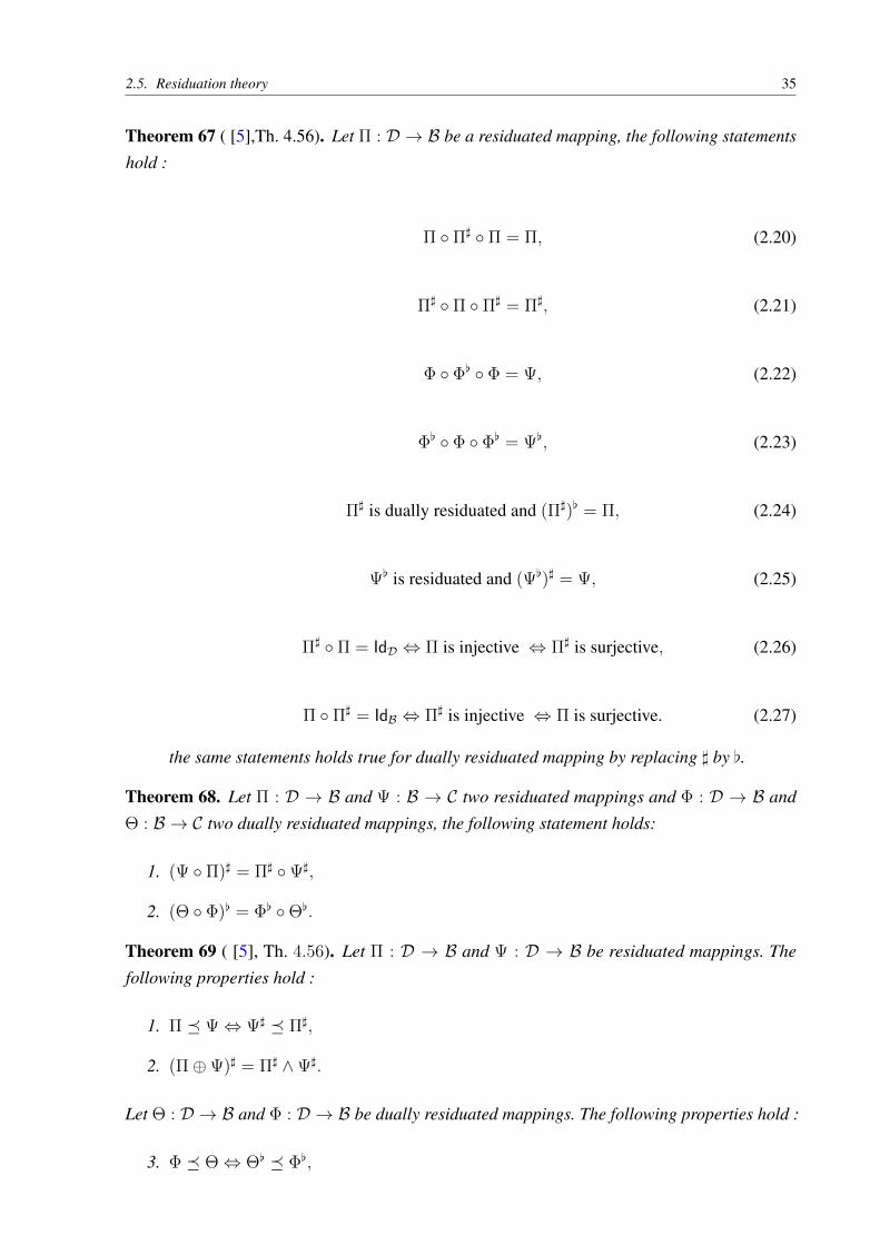
Theorem 67 ( [5],Th. 4.56). Let ⇧ : D ! B be a residuated mapping, the following statementshold :
⇧ � ⇧] � ⇧ = ⇧, (2.20)
⇧
] � ⇧ � ⇧]
= ⇧
], (2.21)
� � �[ � � = , (2.22)
�
[ � � � �[
=
[, (2.23)
⇧
] is dually residuated and (⇧
]
)
[
= ⇧, (2.24)
[ is residuated and (
[
)
]
= , (2.25)
⇧
] � ⇧ = IdD , ⇧ is injective , ⇧
] is surjective, (2.26)
⇧ � ⇧]
= IdB , ⇧
] is injective , ⇧ is surjective. (2.27)
the same statements holds true for dually residuated mapping by replacing ] by [.
Theorem 68. Let ⇧ : D ! B and : B ! C two residuated mappings and � : D ! B and⇥ : B ! C two dually residuated mappings, the following statement holds:
1. ( � ⇧)] = ⇧] � ],
2. (⇥ � �)[ = �[ �⇥[.
Theorem 69 ( [5], Th. 4.56). Let ⇧ : D ! B and : D ! B be residuated mappings. Thefollowing properties hold :
1. ⇧ � ,
] � ⇧],
2. (⇧� )] = ⇧] ^ ].
Let ⇥ : D ! B and � : D ! B be dually residuated mappings. The following properties hold :
3. � � ⇥, ⇥
[ � �[,

36 Chapter 2. Algebraic Preliminaries
4. (� ^⇥)[ = �[ �⇥[.
Theorem 70 ( [8]). Let ⇧ : D ! B and : D ! B be two residuated mappings, then thefollowing equivalence holds :
Im ⇧ ⇢ Im , � ] � ⇧ = ⇧.
Theorem 71 ( [8, 11], Projection on the image of a mapping). Let ⇧ : D ! B be a residuatedmapping, mapping P
⇧
= ⇧ �⇧] is a dual closure mapping. Furthermore P⇧
(b), with b 2 B, isthe greatest element in Im⇧ less than or equal to b.Let : D ! C be a dually residuated mapping, mapping P
= � [ is a closure mapping.Furthermore P
(c), with c 2 C, is the lowest element in Im greater than or equal to c.
Theorem 72 ( [4]). Let C be a complete subsemiring of D. Let Id|C : C ! D, x 7! x bethe canonical injection. The injection Id|C is both residuated and dually residuated and theirresiduals are projectors.
Theorem 73. Let ⇧ : D ! B be a mapping. The following statements hold :
1. if ⇧ is residuated then E|⇧ is residuated, with E such that Im⇧ ⇢ E ⇢ B and
(E|⇧)]
= ⇧
] � Id|E = ⇧
]
|E ;
2. if ⇧ is residuated then ⇧|C is residuated, with C such that Im⇧] ⇢ C ⇢ D and
(⇧|C)]
= C|⇧]
;
3. if ⇧ is dually residuated then E|⇧ is dually residuated, with E such that Im⇧ ⇢ E ⇢ B and
(E|⇧)[
= ⇧
[ � Id|E = ⇧
[
|E ;
4. if ⇧ is dually residuated then ⇧|C is dually residuated, with C such that Im⇧[ ⇢ C ⇢ Dand
(⇧|C)[
= C|⇧[.
Theorem 74 ( [4]). Let ⇧ : D ! D a closure mapping. The restriction Im⇧|⇧ is residuated andits residual is
�Im⇧|⇧
�]
= Id|Im⇧
with Id|Im⇧ the canonical injection of Im⇧ in D.
Example 75. The following mappings are considered :
La
: D ! D: x 7! a⌦ x (left product by a),
Ra
: D ! D: x 7! x⌦ a (right product by a).
(2.28)
2.5. Residuation theory 37
According to semiring definition (see Definition 22) these mappings are l.s.c (La
(x1
� x2
) =
La
(x1
)� La
(x2
)) and such that La
(") = "), hence according to Definition 64 these mappingsare residuated. The residual mappings are denoted :
L]
a
(x) = a�\x (left division by a),
R]
a
(x) = x�/a (right division by a).(2.29)
Example 76 ( [4], [12], [8], [9]). it is possible to show that the following mappings are residuated,with D and C some ordered sets and Cop the dual set C, i.e. the same set endowed with theopposite order (i.e., a �Cop b , a ⌫C b).
⇤
a
: D ! Cop
x 7! x�\a,
a
: Cop ! Dx 7! a�/x.
(2.30)
The residual mappings are given below :
⇤
]
a
=
a
: Cop ! Dx 7! a�/x,
]
a
= ⇤
a
: D ! Cop
x 7! x�\a.
(2.31)
Remark 77. This result shows that the greatest solution in D of inequality x�\a ⌫ b is a�/b, andb�\a is the greatest solution of the inequality a�/x ⌫ b.
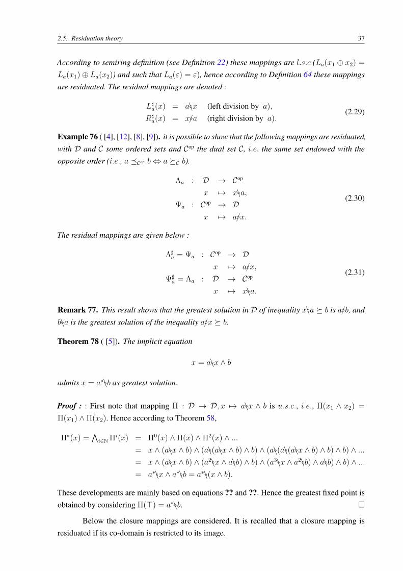
Theorem 78 ( [5]). The implicit equation
x = a�\x ^ b
admits x = a⇤�\b as greatest solution.
Proof : : First note that mapping ⇧ : D ! D, x 7! a�\x ^ b is u.s.c., i.e., ⇧(x1
^ x2
) =
⇧(x1
) ^ ⇧(x2
). Hence according to Theorem 58,
⇧
⇤(x) =
Vi2N⇧
i
(x) = ⇧
0
(x) ^ ⇧(x) ^ ⇧2
(x) ^ ...
= x ^ (a�\x ^ b) ^ (a�\(a�\x ^ b) ^ b) ^ (a�\(a�\(a�\x ^ b) ^ b) ^ b) ^ ...
= x ^ (a�\x ^ b) ^ (a2�\x ^ a�\b) ^ b) ^ (a3�\x ^ a2�\b) ^ a�\b) ^ b) ^ ...
= a⇤�\x ^ a⇤�\b = a⇤�\(x ^ b).
These developments are mainly based on equations ?? and ??. Hence the greatest fixed point isobtained by considering ⇧(>) = a⇤�\b. ⇤
Below the closure mappings are considered. It is recalled that a closure mapping isresiduated if its co-domain is restricted to its image.

38 Chapter 2. Algebraic Preliminaries
Example 79 ( [7]). Mapping S : D ! D, x 7! x⇤ is a closure mapping. Hence (ImS|S) isresiduated and its residual is (ImS|S)
]
= IImS
. In other words, inequality x⇤ � a⇤ admits x = a⇤
as greatest solution.
Example 80 ( [7]). Mapping P : D ! D, x 7!Li�1
xi
= x+ is a closure mapping. Hence (ImP |P )
is residuated and its residual is (ImP |P )
]
= IImP
. In other words, inequality x+ � a+ admitsx = a+ as greatest solution.
Example 81 ( [13]). Isotone mapping Qa
: D ! D, x 7! (xa)⇤x is a closure mapping.Hence ImQ
a
|Qa
is residuated and its residual is (ImQ
a
|Qa
)
]
= IImQ
a
. In otehr words, inequality(xa)⇤x � b, with b 2 ImQ
a
, admits x = b as greatest solution, furthermore the following equlityholds (ba)⇤b = b.
Example 82 ( [7], [14]). Let Mh
: D ! D, x 7! h(xh)⇤ an isotone mapping defined overcomplete idempotent semiring and sets
G1
= {g 2 D | 9a 2 D, g = a⇤h} ,G2
= {g 2 D | 9b 2 D, g = hb⇤} .
It can be shown that G1|Mh
et G2|Mh
are residuated with:
(G1|Mh
)
]
(x) = h�\x�/h,
(G2|Mh
)
]
(x) = h�\x�/h.
Below, it is recalled that the canonical injection from a complete subsemiring into acomplete semiring is residuated.
Theorem 83 (Projection Lemma [4]). Let D be a complete semiring and Dsub
a completesubsemiring of D. The canonical injection ID
sub
: Dsub
! D, x 7! x is residuated. The residualis denoted as PrD
sub
= I]Dsub
and is such that :
(i) PrDsub
� PrDsub
= PrDsub
,
(ii) PrDsub
� IdD,
(iii) x 2 Dsub
() PrDsub
(x) = x.
Proposition 84 ( [7]). Let ⇧ : C ! D a residuated mapping defined over complete idempotentsemiring and IC
sub
the canonical injection of the subsemiring Csub
into C. Mapping⇧�ICsub
(x) �b is residuated and its residual is given by
�⇧|C
sub
�]
(b) = (⇧ � ICsub
)
]
(b) = PrCsub
� ⇧]
(b). (2.32)
2.6. Semiring Zmax
39
Proposition 85. Let ⇧ : C ! D be a residuated mapping defined over complete idempotentsemiring and ID
sub
the canonical injection of the complete subsemiring Dsub
(with Im⇧ ⇢D
sub
⇢ D) into D. Mapping Dsub
|⇧ is residuated and�D
sub
|⇧�]
= ⇧
] � IDsub
=
�⇧
]
�|D
sub
.
The classical kernel definition of a mapping (i.e., set {x|⇧(x) = "}) has a weak sensewhen mappings are defined over lattices. Hence the following definition is classically consideredfor these mappings.
Definition 86 (Kernel). The kernel of mapping C : X ! Y , denoted kerC, is defined by thefollowing equivalence relation
xkerC⌘ x0 () C(x) = C(x0
). (2.33)
This relation defines a congruence. The quotient set X/ kerC
is then the set of equivalence classesmodulo kerC.
Notation 87. An equivalence class of X/ kerC
will be denoted [x]C
.
Proposition 88 ( [15]). If C : X ! Y ia a residuated mapping then each equivalence class [x]C
has one and only one element of ImC], furthermore it is the greatest element of this class.
2.6 Semiring Zmax
This section aims to present the semiring (max,+), denoted Zmax
and already introducedin example 29.
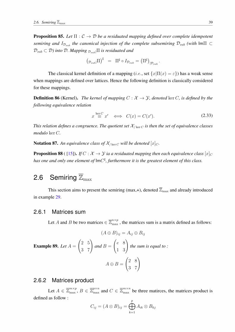
2.6.1 Matrices sum
Let A and B be two matrices 2 Zn⇥p
max
, the matrices sum is a matrix defined as follows:
(A� B)
ij
= Aij
� Bij
Example 89. Let A =
2 5
3 7
!and B =
e 8
1 3
!the sum is equal to :
A� B =
2 8
3 7
!
2.6.2 Matrices product
Let A 2 Zm⇥p
max
, B 2 Zp⇥n
max
and C 2 Zm⇥n
max
be three matirces, the matrices product isdefined as follow :
Cij
= (A⌦ B)
ij
=
pM
k=1
Aik
⌦ Bkj
40 Chapter 2. Algebraic Preliminaries
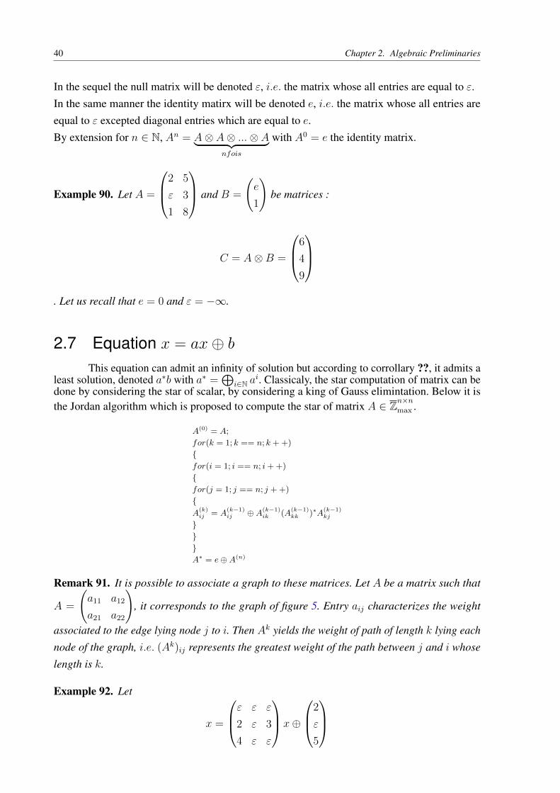
In the sequel the null matrix will be denoted ", i.e. the matrix whose all entries are equal to ".In the same manner the identity matirx will be denoted e, i.e. the matrix whose all entries areequal to " excepted diagonal entries which are equal to e.By extension for n 2 N, An
= A⌦ A⌦ ...⌦ A| {z }nfois
with A0
= e the identity matrix.
Example 90. Let A =
0
B@2 5
" 3
1 8
1
CA and B =
e
1
!be matrices :
C = A⌦ B =
0
B@6
4
9
1
CA
. Let us recall that e = 0 and " = �1.
2.7 Equation x = ax� b
This equation can admit an infinity of solution but according to corrollary ??, it admits aleast solution, denoted a⇤b with a⇤ =
Li2N a
i. Classicaly, the star computation of matrix can bedone by considering the star of scalar, by considering a king of Gauss elimintation. Below it isthe Jordan algorithm which is proposed to compute the star of matrix A 2 Zn⇥n
max
.
A
(0) = A;
for(k = 1; k == n; k ++)
{for(i = 1; i == n; i++)
{for(j = 1; j == n; j ++)
{A
(k)ij
= A
(k�1)ij
�A
(k�1)ik
(A(k�1)kk
)⇤A(k�1)kj
}}}A
⇤ = e�A
(n)
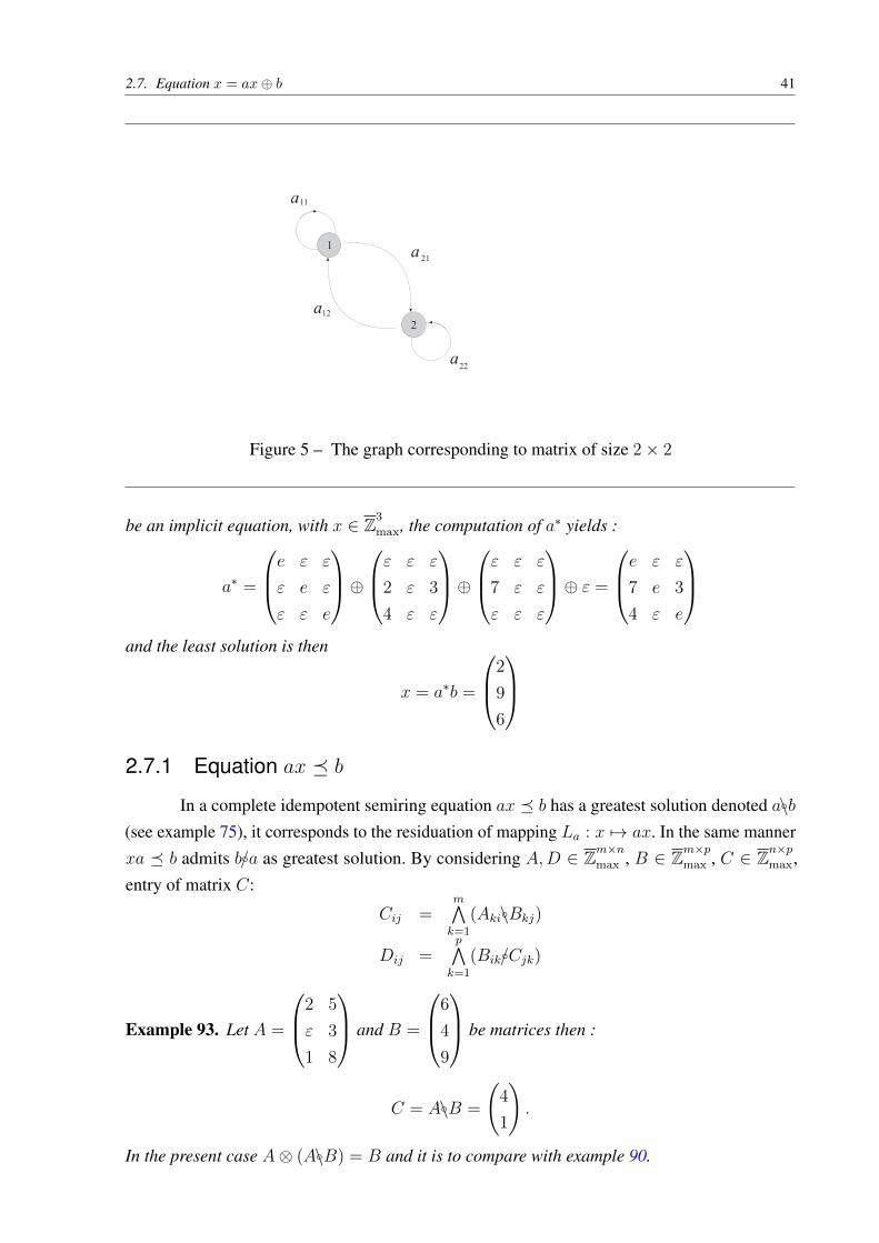
Remark 91. It is possible to associate a graph to these matrices. Let A be a matrix such that
A =
a11
a12
a21
a22
!, it corresponds to the graph of figure 5. Entry a
ij
characterizes the weight
associated to the edge lying node j to i. Then Ak yields the weight of path of length k lying eachnode of the graph, i.e. (Ak
)
ij
represents the greatest weight of the path between j and i whoselength is k.
Example 92. Let
x =
0
B@" " "
2 " 3
4 " "
1
CAx�
0
B@2
"
5
1
CA
2.7. Equation x = ax� b 41
Figure 5 – The graph corresponding to matrix of size 2⇥ 2
be an implicit equation, with x 2 Z3
max
, the computation of a⇤ yields :
a⇤ =
0
B@e " "
" e "
" " e
1
CA�
0
B@" " "
2 " 3
4 " "
1
CA�
0
B@" " "
7 " "
" " "
1
CA� " =
0
B@e " "
7 e 3
4 " e
1
CA
and the least solution is then
x = a⇤b =
0
B@2
9
6
1
CA
2.7.1 Equation ax � b
In a complete idempotent semiring equation ax � b has a greatest solution denoted a�\b(see example 75), it corresponds to the residuation of mapping L
a
: x 7! ax. In the same mannerxa � b admits b�/a as greatest solution. By considering A,D 2 Zm⇥n
max
, B 2 Zm⇥p
max
, C 2 Zn⇥p
max
,entry of matrix C:
Cij
=
mVk=1
(Aki
�\Bkj
)
Dij
=
pVk=1
(Bik
�/Cjk
)
Example 93. Let A =
0
B@2 5
" 3
1 8
1
CA and B =
0
B@6
4
9
1
CA be matrices then :
C = A�\B =
4
1
!.
In the present case A⌦ (A�\B) = B and it is to compare with example 90.
42 Chapter 2. Algebraic Preliminaries
2.7.2 Spectral theory of matrices
Definition 94 (Graphe fortement connexe). A graph is said to be strongly connected if it exists apath between i and j two nodes, 8i, j.
Definition 95 (Irreducible Matrix). Matrix A 2 Zn⇥n
max
is said to be irreductible if the correspond-ing graph is strongly connected, conversely, A is said to be reducible.
Definition 96 (Trace of a matrix). The trace of a matrix is classically defined:
trace(A) =
nM
i=1
(A)ii
.
Remark 97. Remark 91 said that (Aj
)
ii
represents the maximal weight of all the circuit of length
j crossing i. From defintion 96, it comes thatnL
i=1
(Aj
)
ii
= trace(Aj
) is the greatest among all
the weight associated to each node i 2 [1, n].
Definition 98. (trace(Aj
))
(
1j
) corresponds to the mean weight associated to the circuits oflength j.
Definition 99.
� =
nM
j=1
(trace(Aj
))
(
1j
)
is called the maximal mean cycle of matrix A. It is the greatest mean weight for all paths whoselength belongs to [1, n] (n being the maximal length of an elementary circuit).
Definition 100 (Eigen vector, eigen value). Let A 2 Zn⇥n
max
be a matrix, � a scalar, and x 2 Zn
max
a vector. � is an eigen value if :Ax = �x
and x is an eigen vector.
Theorem 101. If A is irreducible, it exists an unique eigen value. It is equal to the greates meancycle of matrix A.
Example 102. Let A =
0
BBBB@
2 5 " "
" " 3 3
e " " "
" e " "
1
CCCCAbe a matrix, the greatest mean cycle of this irreducible
matrix is equal to � = 8/3.
43
3 System Modelling and Control Theory
3.1 Model for systems subject to synchronization and de-
lay
3.1.1 Daters equations, the event point of view
In the beginning of the 60th Cuninghame-Green started to represent manufacturingsystem in (max, plus) algebra. In the very beginning of the 80th, a team of INRIA Rocquencourtwas interested by the description of Timed Event Graphs (TEGs) in (max, plus) algebra (seee.g. [16]. TEGs constitute a subclass of timed Petri nets whose each place admits one and onlyone upstream transition and one and only one downstream transition.
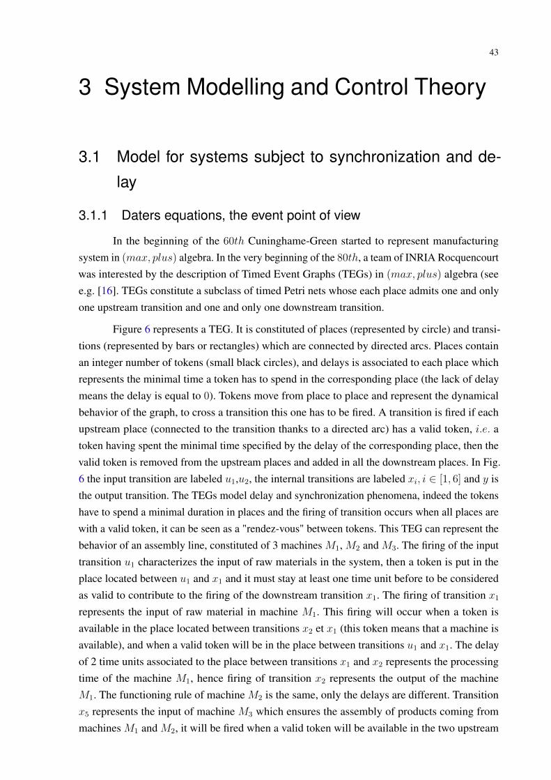
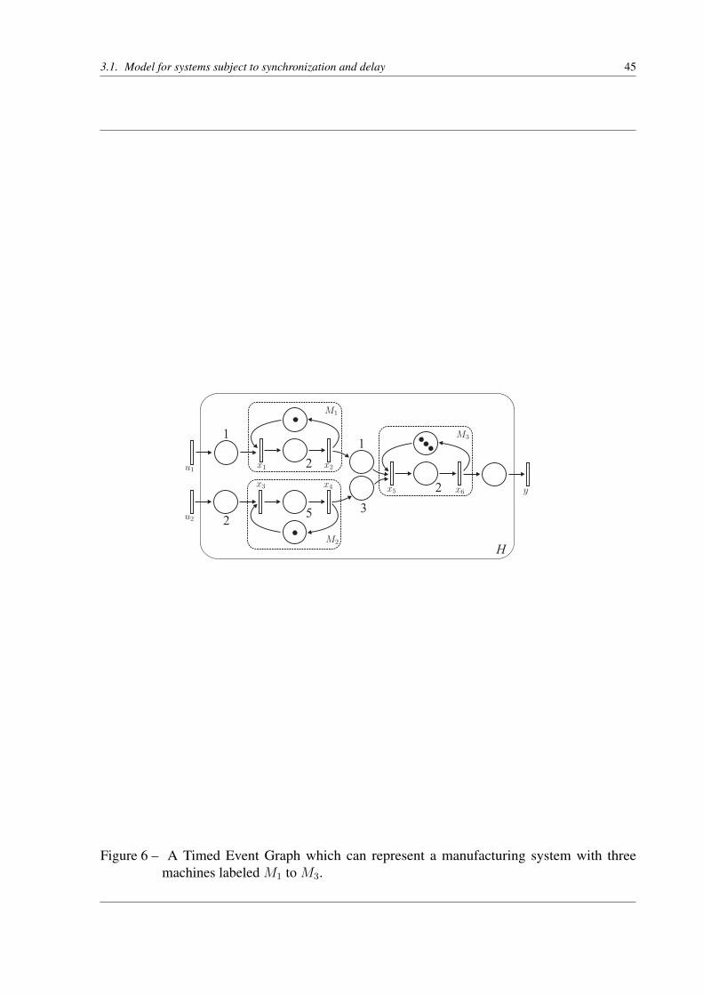
Figure 6 represents a TEG. It is constituted of places (represented by circle) and transi-tions (represented by bars or rectangles) which are connected by directed arcs. Places containan integer number of tokens (small black circles), and delays is associated to each place whichrepresents the minimal time a token has to spend in the corresponding place (the lack of delaymeans the delay is equal to 0). Tokens move from place to place and represent the dynamicalbehavior of the graph, to cross a transition this one has to be fired. A transition is fired if eachupstream place (connected to the transition thanks to a directed arc) has a valid token, i.e. atoken having spent the minimal time specified by the delay of the corresponding place, then thevalid token is removed from the upstream places and added in all the downstream places. In Fig.6 the input transition are labeled u
1
,u2
, the internal transitions are labeled xi
, i 2 [1, 6] and y isthe output transition. The TEGs model delay and synchronization phenomena, indeed the tokenshave to spend a minimal duration in places and the firing of transition occurs when all places arewith a valid token, it can be seen as a "rendez-vous" between tokens. This TEG can represent thebehavior of an assembly line, constituted of 3 machines M
1
, M2
and M3
. The firing of the inputtransition u
1
characterizes the input of raw materials in the system, then a token is put in theplace located between u
1
and x1
and it must stay at least one time unit before to be consideredas valid to contribute to the firing of the downstream transition x
1
. The firing of transition x1
represents the input of raw material in machine M1
. This firing will occur when a token isavailable in the place located between transitions x
2
et x1
(this token means that a machine isavailable), and when a valid token will be in the place between transitions u
1
and x1
. The delayof 2 time units associated to the place between transitions x
1
and x2
represents the processingtime of the machine M
1
, hence firing of transition x2
represents the output of the machineM
1
. The functioning rule of machine M2
is the same, only the delays are different. Transitionx5
represents the input of machine M3
which ensures the assembly of products coming frommachines M
1
and M2
, it will be fired when a valid token will be available in the two upstream

44 Chapter 3. System Modelling and Control Theory
transitions. This machine is able to process three parts simultaneously.
The idea of [16, 17] was to show that these dynamical systems which are, a priori nonlinear, can be represented by a linear system of equations in a specific algebraic structure. Inparticular they showed a TEG admits a canonical linear model in (max, plus) algebra. Thedynamical model considered is given below and is very reminiscent to the one of classicaldynamical linear system :
x(k) = Ax(k � 1)� Bu(k) (3.1a)
y(k) = Cx(k) (3.1b)
To obtain this model a dater function is associated to each transition, this function aims to datethe occurrence of the firing of the corresponding transitions (it means that the event point of viewis considered). It will represent the life of the transition. Formally for transition x
j
, the followingfunction is considered : Z ! Z, k 7! x
j
(k) where xj
(k) is the date of the firing of the tokennumbered k.
For the TEG of Fig. 6, this yields :
x1
(k) = max(1 + u1
(k), x2
(k � 1))
x2
(k) = 2 + x1
(k)
x3
(k) = max(2 + u2
(k), x4
(k � 1))
x4
(k) = 5 + x3
(k)
x5
(k) = max(3 + x4
(k), 1 + x2
(k), x6
(k � 3))
x6
(k) = 2 + x5
(k)
y(k) = x6
(k)
(3.2)
The operator plus models the delay and the operator max models the synchronization betweentwo dater functions. These non-linear equations become linear equations in the idempotentsemiring Z
max
(cf. definition 29), then :
x1
(k) = 1⌦ u1
(k)� x2
(k � 1)
x2
(k) = 2⌦ x1
(k)
x3
(k) = 2⌦ u2
(k)� x4
(k � 1)
x4
(k) = 5⌦ x3
(k)
x5
(k) = 3⌦ x4
(k)� 1⌦ x2
(k)� x6
(k � 3)
x6
(k) = 2⌦ x5
(k)
y(k) = x6
(k)
(3.3)
3.1. Model for systems subject to synchronization and delay 45
Figure 6 – A Timed Event Graph which can represent a manufacturing system with threemachines labeled M
1
to M3
.

46 Chapter 3. System Modelling and Control Theory
or, by considering vector notation, and vector state : x(k) =⇣x1
(k) x2
(k) x3
(k) x4
(k) x5
(k) x6
(k)⌘t
,
input vector u(k) =⇣u1
(k) u2
(k)⌘t
and output vector y(k) = (y(k)) :
x(k) =
0
BBBBBBB@
" " " " " "
2 " " " " "
" " " " " "
" " 5 " " "
" 1 " 3 " "
" " " " 2 "
1
CCCCCCCA
x(k)�
0
BBBBBBB@
" 0 " " " "
" " " " " "
" " " 0 " "
" " " " " "
" " " " " "
" " " " " "
1
CCCCCCCA
x(k� 1)�
0
BBBBBBB@
" " " " " "
" " " " " "
" " " " " "
" " " " " "
" " " " " "
" " " " " "
1
CCCCCCCA
x(k� 2)
�
0
BBBBBBB@
" " " " " "
" " " " " "
" " " " " "
" " " " " "
" " " " " 0
" " " " " "
1
CCCCCCCA
x(k � 3)�
0
BBBBBBB@
1 "
" "
" 2
" "
" "
" "
1
CCCCCCCA
u(k)
y(k) =⇣" " " " " 0
⌘x(k)
In a general manner, the model is obtained under the following formalism over Zmax
:
x(k) =
aLi=0
Ai
x(k � i)�bL
j=0
Bj
u(k � j),
y(k) =
cLl=0
Cl
x(k � l).
After some modifications, it is possible to obtain an explicit form with a recurrence of 1 on thevector state. The system admits then the following formalism :
x(k) = A0
x(k)� A1
x(k � 1)� B0
u(k),
y(k) = C0
x(k).
Practically, this is obtained by enlarging the graph in order to guarantee that each placebe initially with at the most one token, figure 7 yields an extension of the TEG of figure 6, andleads to the model :
x(k) =
0
BBBBBBBBBBBB@
" " " " " " " "
2 " " " " " " "
" " " " " " " "
" " 5 " " " " "
" 1 " 3 " " " "
" " " " 2 " " "
" " " " " " " "
" " " " " " " "
1
CCCCCCCCCCCCA
x(k)�
0
BBBBBBBBBBBB@
" e " " " " " "
" " " " " " " "
" " " e " " " "
" " " " " " " "
" " " " " " " e
" " " " " " " "
" " " " " e " "
" " " " " " e "
1
CCCCCCCCCCCCA
x(k � 1)�
0
BBBBBBBBBBBB@
1 "
" "
" 2
" "
" "
" "
" "
" "
1
CCCCCCCCCCCCA
u(k)
y(k) =⇣" " " " " 0 " "
⌘x(k)
Equation (3.1.3.1) is an implicit equation with x(k).
x(k) = Ax(k � 1)� Bu(k) (3.4)
y(k) = Cx(k) (3.5)

3.1. Model for systems subject to synchronization and delay 47
Figure 7 – Example an assembly line (event extension).
48 Chapter 3. System Modelling and Control Theory
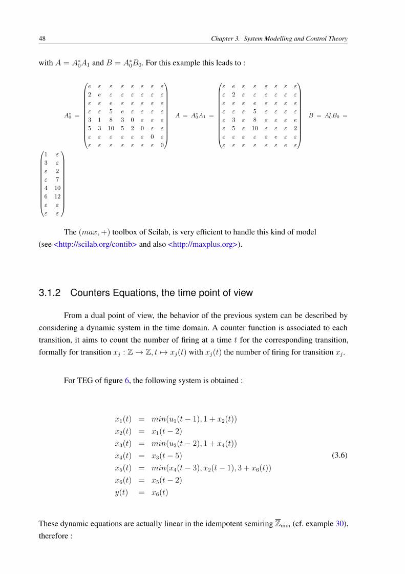
with A = A⇤0
A1
and B = A⇤0
B0
. For this example this leads to :
A
⇤0 =
0
BBBBBBBBBBBB@
e " " " " " " "
2 e " " " " " "
" " e " " " " "
" " 5 e " " " "
3 1 8 3 0 " " "
5 3 10 5 2 0 " "
" " " " " " 0 "
" " " " " " " 0
1
CCCCCCCCCCCCA
A = A
⇤0A1 =
0
BBBBBBBBBBBB@
" e " " " " " "
" 2 " " " " " "
" " " e " " " "
" " " 5 " " " "
" 3 " 8 " " " e
" 5 " 10 " " " 2
" " " " " e " "
" " " " " " e "
1
CCCCCCCCCCCCA
B = A
⇤0B0 =
0
BBBBBBBBBBBB@
1 "
3 "
" 2
" 7
4 10
6 12
" "
" "
1
CCCCCCCCCCCCA
The (max,+) toolbox of Scilab, is very efficient to handle this kind of model(see <http://scilab.org/contib> and also <http://maxplus.org>).
3.1.2 Counters Equations, the time point of view
From a dual point of view, the behavior of the previous system can be described byconsidering a dynamic system in the time domain. A counter function is associated to eachtransition, it aims to count the number of firing at a time t for the corresponding transition,formally for transition x
j
: Z ! Z, t 7! xj
(t) with xj
(t) the number of firing for transition xj
.
For TEG of figure 6, the following system is obtained :
x1
(t) = min(u1
(t� 1), 1 + x2
(t))
x2
(t) = x1
(t� 2)
x3
(t) = min(u2
(t� 2), 1 + x4
(t))
x4
(t) = x3
(t� 5)
x5
(t) = min(x4
(t� 3), x2
(t� 1), 3 + x6
(t))
x6
(t) = x5
(t� 2)
y(t) = x6
(t)
(3.6)
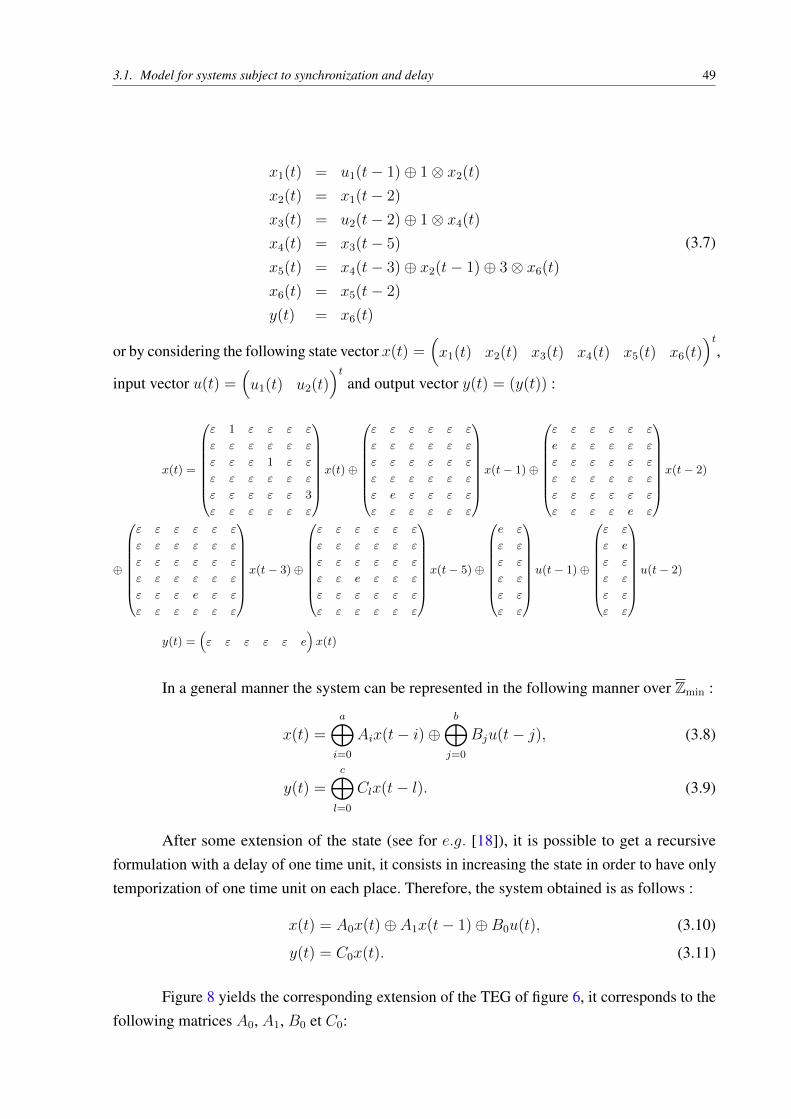
These dynamic equations are actually linear in the idempotent semiring Zmin
(cf. example 30),therefore :
3.1. Model for systems subject to synchronization and delay 49
x1
(t) = u1
(t� 1)� 1⌦ x2
(t)
x2
(t) = x1
(t� 2)
x3
(t) = u2
(t� 2)� 1⌦ x4
(t)
x4
(t) = x3
(t� 5)
x5
(t) = x4
(t� 3)� x2
(t� 1)� 3⌦ x6
(t)
x6
(t) = x5
(t� 2)
y(t) = x6
(t)
(3.7)
or by considering the following state vector x(t) =⇣x1
(t) x2
(t) x3
(t) x4
(t) x5
(t) x6
(t)⌘t
,
input vector u(t) =⇣u1
(t) u2
(t)⌘t
and output vector y(t) = (y(t)) :
x(t) =
0
BBBBBBB@
" 1 " " " "
" " " " " "
" " " 1 " "
" " " " " "
" " " " " 3
" " " " " "
1
CCCCCCCA
x(t)�
0
BBBBBBB@
" " " " " "
" " " " " "
" " " " " "
" " " " " "
" e " " " "
" " " " " "
1
CCCCCCCA
x(t� 1)�
0
BBBBBBB@
" " " " " "
e " " " " "
" " " " " "
" " " " " "
" " " " " "
" " " " e "
1
CCCCCCCA
x(t� 2)
�
0
BBBBBBB@
" " " " " "
" " " " " "
" " " " " "
" " " " " "
" " " e " "
" " " " " "
1
CCCCCCCA
x(t� 3)�
0
BBBBBBB@
" " " " " "
" " " " " "
" " " " " "
" " e " " "
" " " " " "
" " " " " "
1
CCCCCCCA
x(t� 5)�
0
BBBBBBB@
e "
" "
" "
" "
" "
" "
1
CCCCCCCA
u(t� 1)�
0
BBBBBBB@
" "
" e
" "
" "
" "
" "
1
CCCCCCCA
u(t� 2)
y(t) =⇣" " " " " e
⌘x(t)
In a general manner the system can be represented in the following manner over Zmin
:
x(t) =
aM
i=0
Ai
x(t� i)�bM
j=0
Bj
u(t� j), (3.8)
y(t) =
cM
l=0
Cl
x(t� l). (3.9)
After some extension of the state (see for e.g. [18]), it is possible to get a recursiveformulation with a delay of one time unit, it consists in increasing the state in order to have onlytemporization of one time unit on each place. Therefore, the system obtained is as follows :
x(t) = A0
x(t)� A1
x(t� 1)� B0
u(t), (3.10)
y(t) = C0
x(t). (3.11)
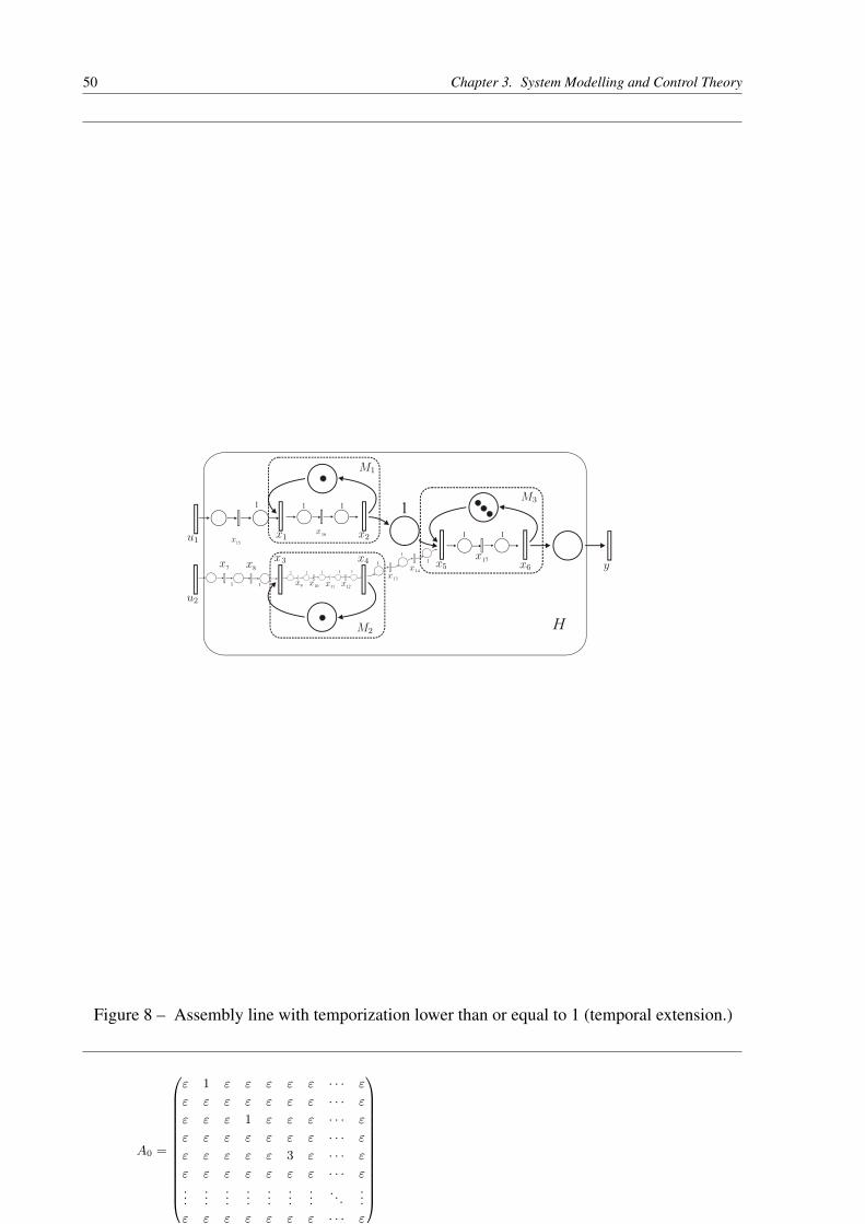
Figure 8 yields the corresponding extension of the TEG of figure 6, it corresponds to thefollowing matrices A
0
, A1
, B0
et C0
:
50 Chapter 3. System Modelling and Control Theory
Figure 8 – Assembly line with temporization lower than or equal to 1 (temporal extension.)
A0 =
0
BBBBBBBBBBBBB@
" 1 " " " " " · · · "
" " " " " " " · · · "
" " " 1 " " " · · · "
" " " " " " " · · · "
" " " " " 3 " · · · "
" " " " " " " · · · "
......
......
......
.... . .
..." " " " " " " · · · "
1
CCCCCCCCCCCCCA
3.1. Model for systems subject to synchronization and delay 51
A1 =
0
BBBBBBBBBBBBBBBBBBBBBBBBBBBBBBBBB@
" " " " " " " "
" " " " " " " "
" " " " " " " e
" " " " " " " "
" e " " " " " "
" " " " " " " "
" " " " " " " "
" " " " " " e "
" " e " " " " "
" " " " " " " "
" " " " " " " "
" " " " " " " "
" " " e " " " "
" " " " " " " "
" " " " " " " "
e " " " " " " "
" " " " e " " "
" " " " " " e " "
" " " " " " " e "
" " " " " " " " "
" " " e " " " " "
" " " " " e " " "
" " " " " " " " e
" " " " " " " " "
" " " " " " " " "
" " " " " " " " "
e " " " " " " " "
" e " " " " " " "
" " e " " " " " "
" " " " " " " " "
" " " " " " " " "
" " " " e " " " "
" " " " " " " " "
" " " " " " " " "
1
CCCCCCCCCCCCCCCCCCCCCCCCCCCCCCCCCA
B =
0
BBBBBBBBBBBBBBBBBBBBBBBBBBBBBBBBB@
" "
" "
" "
" "
" "
" "
" e
" "
" "
" "
" "
" "
" "
" "
e "
" "
" "
" " " " " " e " "
" " " " " " " e "
" " " " " " " " "
" " " e " " " " "
" " " " " e " " "
" " " " " " " " e
" " " " " " " " "
" " " " " " " " "
" " " " " " " " "
e " " " " " " " "
" e " " " " " " "
" " e " " " " " "
" " " " " " " " "
" " " " e " " " "
" " " " " " " " "
" " " " " " " " "
" " " " " " " " "
1
CCCCCCCCCCCCCCCCCCCCCCCCCCCCCCCCCA
C =⇣" " " " " e " " " " " " " " " " "
⌘
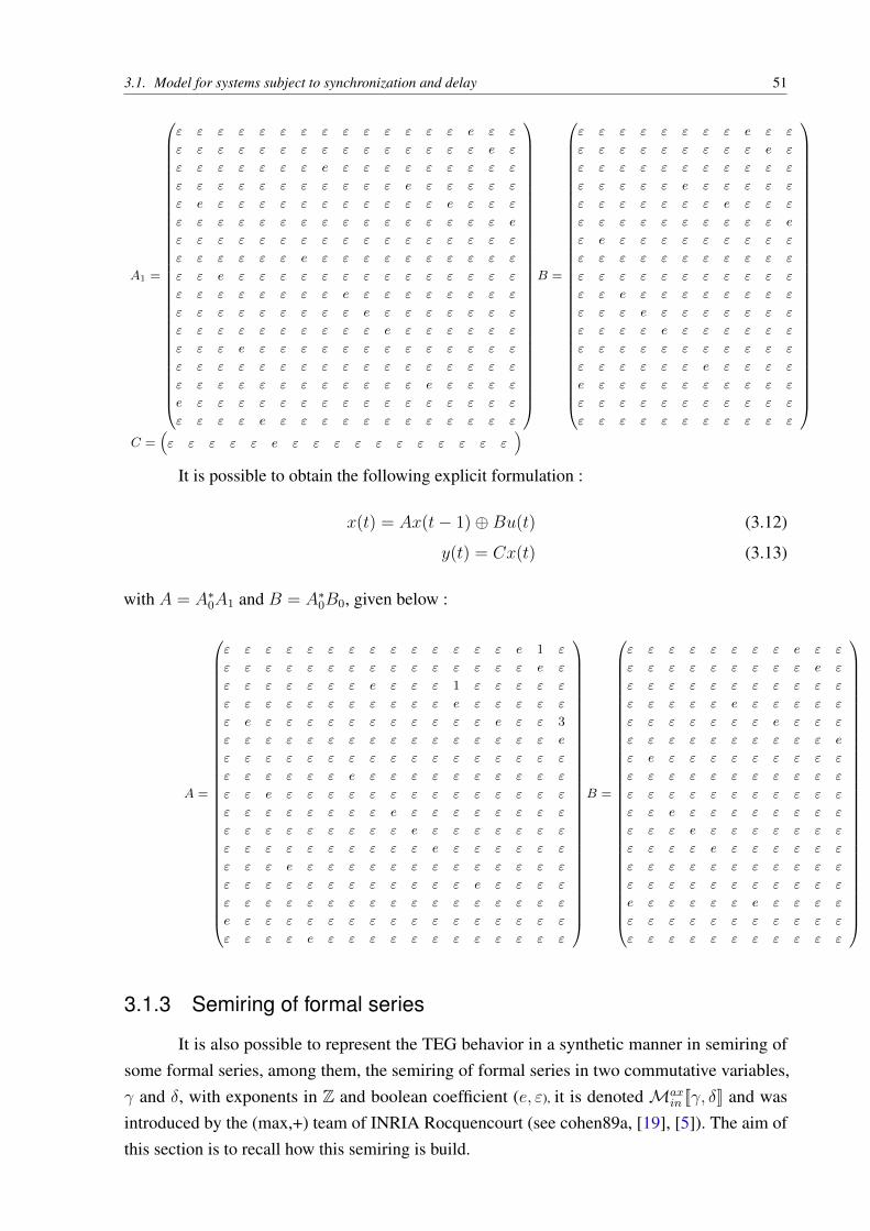
It is possible to obtain the following explicit formulation :
x(t) = Ax(t� 1)� Bu(t) (3.12)
y(t) = Cx(t) (3.13)
with A = A⇤0
A1
and B = A⇤0
B0
, given below :
A =
0
BBBBBBBBBBBBBBBBBBBBBBBBBBBBBBBBB@
" " " " " " " "
" " " " " " " "
" " " " " " " e
" " " " " " " "
" e " " " " " "
" " " " " " " "
" " " " " " " "
" " " " " " e "
" " e " " " " "
" " " " " " " "
" " " " " " " "
" " " " " " " "
" " " e " " " "
" " " " " " " "
" " " " " " " "
e " " " " " " "
" " " " e " " "
" " " " " " e 1 "
" " " " " " " e "
" " " 1 " " " " "
" " " e " " " " "
" " " " " e " " 3
" " " " " " " " e
" " " " " " " " "
" " " " " " " " "
" " " " " " " " "
e " " " " " " " "
" e " " " " " " "
" " e " " " " " "
" " " " " " " " "
" " " " e " " " "
" " " " " " " " "
" " " " " " " " "
" " " " " " " " "
1
CCCCCCCCCCCCCCCCCCCCCCCCCCCCCCCCCA
B =
0
BBBBBBBBBBBBBBBBBBBBBBBBBBBBBBBBB@
" "
" "
" "
" "
" "
" "
" e
" "
" "
" "
" "
" "
" "
" "
e "
" "
" "
" " " " " " e " "
" " " " " " " e "
" " " " " " " " "
" " " e " " " " "
" " " " " e " " "
" " " " " " " " e
" " " " " " " " "
" " " " " " " " "
" " " " " " " " "
e " " " " " " " "
" e " " " " " " "
" " e " " " " " "
" " " " " " " " "
" " " " " " " " "
" " " " e " " " "
" " " " " " " " "
" " " " " " " " "
1
CCCCCCCCCCCCCCCCCCCCCCCCCCCCCCCCCA
3.1.3 Semiring of formal series
It is also possible to represent the TEG behavior in a synthetic manner in semiring ofsome formal series, among them, the semiring of formal series in two commutative variables,� and �, with exponents in Z and boolean coefficient (e, "), it is denoted Max
in
[[�, �]] and wasintroduced by the (max,+) team of INRIA Rocquencourt (see cohen89a, [19], [5]). The aim ofthis section is to recall how this semiring is build.

52 Chapter 3. System Modelling and Control Theory
3.1.3.1 Semiring Zmax
[[�]]
Definition 103. The � transform of a signal is defined as follow :
d(�) =M
i2Z
d(k)⌦ �k
Remark 104. This transform is analogous to the z transform of the classical system theorywhich allows to code a discrete trajectory by a formal series.
Remark 105. Since � ⌦ d(�) =Li2Z
d(k) ⌦ �k+1
=
Li2Z
d(k � 1) ⌦ �k, the � operator can be
seen as a backward shift operator, i.e., x(k � 1) = �x(k).
Definition 106 (Semiring Zmax
[[�]]). The set of formal series in � with exponents in Z andcoefficients in Z
max
has an idempotent semiring structure. The neutral element of the additionis the series defined as : " =
Li2Z
"�k (where " = �1 is the neutral element of the sum in
Zmax
). The neutral element of the product law is the formal series e(�) = e�0 (where e = 0 isthe neutral element of the product law in Z
max
). The sum and the product (actually a Cauchyproduct) are defined as follows :
d1
(�)� d2
(�) =
Lk2Z(d1(k)� d
2
(k))�k
d1
(�)⌦ d2
(�) =
Lj2Z(d1(j)� d
2
(k � j))�k
System 3.4 in Zmax
, can be easily translated in Zmax
[[�]] :
x(�) = �Ax(�)� Bu(�)
y = Cx(�)
A transfer relation can be computed it represents the input/output behavior of the system:
y(�) = C(�A)⇤Bu(�) = Hu(�)
It is also possible to consider model 3.1.3.1 in idempotent semiring Zmax
[[�]] :
x(�) =
aLi=0
�iAi
x(�)�bL
j=0
�jBj
u(�),
y(�) =
cLl=0
�lCl
x(�).
leading to the following model :
x(�) = Ax(�)� Bu(�)
y = Cx(�)
with A =
aLi=0
�iAi
, B =
bLj=0
�jBj
et C =
cLl=0
�lCl
. Entries of matrices A,B and C are then
polynomials. This formulation is not in a standard way, but it is then not necessary to increasethe state vector size. In the following this kind of model will be consider, but the reader shouldhave in mind that it can get easily a standard form.
3.1. Model for systems subject to synchronization and delay 53
3.1.3.2 Monotonic Trajectories
The trajectories which are solutions of the previous systems are not necessarily monotone,nevertheless the firing sequence associated to a transition of a TEG is not decreasing (theoccurrence date d(k) of the firing k is necessarily greater than or equal to d(k � 1)). Formally,
8k 2 Z d(k) � d(k � 1) , d(k) = d(k)� d(k � 1).
is equivalent tod(�) = d(�)� �d(�) , d(�) = �⇤d(�).
This means that the � transform of a monotonic trajectory can be written as �⇤d(�) andthat the multiplication by �⇤ of a non monotonic trajectory yields a monotonic non decreasingtrajectory. It is a kind of filter. The set of monotonic trajectories (i.e., which can be written�⇤d(�)) is an idempotent sub semiring Z
max
[[�]], it is denoted �⇤Zmax
[[�]]. Indeed it easy to checkthat the sum and the product of non decreasing element is non decreasing, then they are closedoperations, and obviously the series e and " are non decreasing. In the sequel the product by �⇤
will be omitted but as we will handle non decreasing trajectories the equality will have to beunderstood "modulo �⇤". For instance :
3� � 1�7 � 5�9
= 3� � 5�9
In general manner the following simplifiaction rules will be considered :
�n � �n
0= �min(n,n
0)
The neutral element for the multiplication of the semiring �⇤Zmax
[[�]] is then the series e(�) =e� e� � e�2 � ...� e�+1. The neutral element for the addition of �⇤Z
max
[[�]] is then "(�) =
"� "� � "�2 � ...� "�+1, with " = �1 the neutral element of the addition of Zmax
.
Remark 107. In the sequel only monotonic series will be handle. Hence, in order to lighten thenotations, without ambiguity , Z
max
[[�]] must be understood as �⇤Zmax
[[�]].
3.1.3.3 Semiring Zmin
[[�]]
In a dual manner it is possible to define a transform for the trajectories considered in thetemporal domain.
Definition 108. The � transform od a signal is defined as follows :
d(�) =M
t2Z
c(t)⌦ �t
Definition 109 (Semiring Zmin
[[�]]). The set of formal series in � with exponents in Z anscoefficients in Z
min
has an idempotent semiring. The neutral element of the addition is the series
54 Chapter 3. System Modelling and Control Theory
" =Lt2Z
"�t (where " = +1 is the neutral element of the addition in Zmin
). The neutral element
of the multiplication is series e(�) = e�0 (where e = 0 is the neutral element of the multiplicationof Z
min
). The sum and the product (Cauchy product) of formal series are defined as follows :
c1
(�)� c2
(�) =
Lt2Z(c1(t)� c
2
(t))�t
c1
(�)⌦ c2
(�) =
Lj2Z(c1(j)� c
2
(t� j))�t
The system of equations 3.12 corresponds to the standardized model in the semiringZ
min
and can be transposed in the semiring Zmin
[[�]] :
x(�) = �Ax(�)� Bu(�)
y = Cx(�)
The input/output transfer relation can be computed :
y(�) = C(�A)⇤Bu(�) = Hu(�)
In an equivalent manner, it is possible to consider the system under the form given byequation 3.1.3.1 in Z
min
[[�]] :
x(�) =
aLi=0
�iAi
x(�)�bL
j=0
�jBj
u(�),
y(�) =
cLl=0
�lCl
x(�).
leading to the following model:
x(�) = Ax(�)� Bu(�)
y = Cx(�)
with A =
aLi=0
�iAi
, B =
bLj=0
�jBj
et C =
cLl=0
�lCl
. The elements of matrices A,B and C are then
polynomials.
3.1.3.4 Monotonic trajectories
As in the event domain the trajectories corresponding to the firing of transitions ot TEGare monotonics (the number of events occurring at time (t+ 1), c(t+ 1), is necessarily greaterthan or equal to the number of firing being occurred at time t, c(t)). Formally,
8t 2 Z c(t) ⌫ c(t+ 1) , c(t) = c(t+ 1)� c(t).
this is equivalent to
c(�) = ��1c(�)� c(�) , c(�) = (��1
)
⇤c(�).

3.1. Model for systems subject to synchronization and delay 55
This means that the � transform of a monotonic trajectory belongs to semiring (��1
)
⇤Zmin
[[�]].The following simplification rules are then considered:
�t � �t0
= �max(t,t
0)
The neutral element of the multiplication law (��1
)
⇤Zmin
[[�]] is series e(�) = e� e�� e�2� ...�e�+1. The neutral element for the addition (��1
)
⇤Zmin
[[�]] is series "(�) = "� "�1 � "�2 � ...�"�+1, with " = +1 the neutral element of the addition of Z
min
.
3.1.4 Two-dimensionnal description, semiring Max
in
[[�, �]]
The choose between the temporal and the event domain will be driven by the applications.Then it can be useful to keep the ability to switch between the two point of view by consideringa two-dimensional description of trajectories. Below the construction of a semiring of formalseries with two commutative variables, � and �, with exponents in Z and with boolean coefficient.For the example of figure 6 the following equation is obtained :
0
BBBBBBBBB@
x1
x2
x3
x4
x5
x6
1
CCCCCCCCCA
=
0
BBBBBBBBB@
" � " " " "
�2 " " " " "
" " " � " "
" " �5 " " "
" � " �3 " �3
" " " " �2 "
1
CCCCCCCCCA
0
BBBBBBBBB@
x1
x2
x3
x4
x5
x6
1
CCCCCCCCCA
�
0
BBBBBBBBB@
� "
" "
" �2
" "
" "
" "
1
CCCCCCCCCA
u1
u2
!
y =
⇣" " " " " e
⌘
0
BBBBBBBBB@
x1
x2
x3
x4
x5
x6
1
CCCCCCCCCA
(3.14)
corresponding to the following standard formalism :
x = Ax� Bu
y = Cx.(3.15)
To each transition of the TEG is associated an entry of the vector x 2 Max
in
[[�, �]]n (vectorcorresponding to the internal transitions, in this example n = 6), u 2 Max
in
[[�, �]]m (vectorcorresponding to the inputs transitions, inthis example m = 2) and y 2 Max
in
[[�, �]]l (vectorassociated to output transitions, in this example l = 1). Matrices A 2 Max
in
[[�, �]]n⇥n, B 2Max
in
[[�, �]]n⇥m, C 2 Max
in
[[�, �]]l⇥n, represents the interaction between transitions. The matricesentries are polynomials of Max
in
[[�, �]]. Entry A5,6
= �3 means that 3 tokens are in the placebetween x
6
and x5
, in a dually manner, entry A4,3
= �5 means that a temporization of 5 times

56 Chapter 3. System Modelling and Control Theory
units is associated to the place between transitions x3
and x4
.By solving the implicit equation, by considering the result on fixed point equations, an input/ouputtransfer relation is obtained. In this example, the transfer matrix denoted H 2 Max
in
[[�, �]]l⇥m isgiven by :
H = CA⇤B =
⇣�6(��2)⇤ �12(��5)⇤
⌘. (3.16)
In a genaral manner, the entries of the transfer matrix representing a TEG are periodicand causal series, which can be written in the following standardized form : p � qr⇤, with p
and q polynomials with exponents in N and r a monomial with exponents in N. Polynomialp characterizes the transient behavior of the series, polynomial q represents a pattern whichis repeated periodically, the periodicity is given by r = �⌫�⌧ where ⌫/⌧ corresponds to theproduction rate of the series, conversely ⌧/⌫ is the cycle time of the series. An example ofperiodic seriesis given on figure 9.To summarize a TEG admits a model in the subsemiring of periodic and causal series.
3.2 Control Theory
3.2.1 State feedback controller synthesis
State feedback controller synthesis is now considered, the reader interested shouldconsult [14]. The architecture considered is given in figure 10, its state representation is given by: (
x = Ax� Bu
y = Cx(3.17)
with A 2 Max
in
[[�, �]]n⇥n, B 2 Max
in
[[�, �]]n⇥m and C 2 Max
in
[[�, �]]l⇥n. The control is given bythe following expression :
u = Kx� v
with K 2 Max
in
[[�, �]]m⇥n. The system becomes(
x = Ax� B(Kx� v)
y = Cx)(
x = (A� BK)x� Bv
y = Cx
and the input/output transfer relation with controller K is :
y = C(A� BK)
⇤Bv = GK
v.
GK
= CA⇤(A⇤BK)
⇤A⇤B
= CA⇤B(KA⇤B)
⇤.
The objective is to synthesize the greatest controller K, such that GK
� Gref
. Theoptimal controller exists if G
ref
2 G1
, it is given by (see [14] for the proof) : :
Kopt
= (H�\Gref
�/A⇤B). (3.18)
3.2. Control Theory 57
Remark 110. It must be noted that the output feedback controller and the state feedbackcontroller are linked as follows :
Fopt
= Kopt
�/C
c.-à-d. Fopt
C = (Kopt
�/C)C � Kopt
. It comes (Fopt
H)
⇤= (F
opt
CA⇤B)
⇤ � (Kopt
A⇤B)
⇤ )CA⇤B(F
opt
CA⇤B)
⇤= G
F
opt
� CA⇤B(Kopt
A⇤B)
⇤= G
K
opt
. In other words, the measurementof all the state improves the efficiency of the control, c.-à-d. leads to a greater control and acorrected system closer to the reference model.
3.2.2 Observer synthesis
In this section the synthesis of an observer allowing to get an estimation of unmeasuredstate is proposed. It is done in an analoguous manner to the one of the classical linear systems(i.e. observer in the Luenberger sense (see [20]). The architecture considered is given in Figure11.
Matrices A, B, C and R are assumed to beknown. Without lost of generality, the rows ofmatrix C are such that only one entry is different of " and that this entry is equal to e. Practicallyeach row of matric C allows to connect one state to the output, it then represents the locationof sensors yielding information of some state. The system is characterized by the followingequations :
x = Ax� Bu�Rw = A⇤Bu� A⇤Rw (3.19)
y = Cx = CA⇤Bu� CA⇤Rw
and the observer can be written as follows :
x = Ax� Bu� L(y � y)
= Ax� Bu� LCx� LCx (3.20)
y = Cx.
By introducing equation (3.19) and by solving the implicit equation, these equations(3.20) become :
x = (A� LC)
⇤Bu� (A� LC)
⇤LCA⇤Bu� (A� LC)
⇤LCA⇤Rw. (3.21)
By considering (2.14), the following equality is obtained :
(A� LC)
⇤= A⇤
(LCA⇤)
⇤, (3.22)
58 Chapter 3. System Modelling and Control Theory
by introducing it in equation (3.21), the following state estimation appears :
x = A⇤(LCA⇤
)
⇤Bu� A⇤(LCA⇤
)
⇤LCA⇤Bu� A⇤(LCA⇤
)
⇤LCA⇤Rw,
by recalling that (LCA⇤)
⇤LCA⇤= (LCA⇤
)
+, this equation becomes:
x = A⇤(LCA⇤
)
⇤Bu� A⇤(LCA⇤
)
+Bu� A⇤(LCA⇤
)
+Rw.
From equation (2.9), it comes (LCA⇤)
⇤ ⌫ (LCA⇤)
+, hence the observer equation can be written:
x = A⇤(LCA⇤
)
⇤Bu� A⇤(LCA⇤
)
+Rw
= (A� LC)
⇤Bu� (A� LC)
⇤LCA⇤Rw. (3.23)
(3.24)
The goal of the observer synthesis is to compute the greatest observer matrix L such thatthe estimated vector
x be as close as possible to state x, by respecting the following constraint x � x, formallythis can be written as follows :
(A� LC)
⇤Bu� (A� LC)
⇤LCA⇤Rw � A⇤Bu� A⇤Rw 8(u, w)
or in an equivalent manner :
(A� LC)
⇤B � A⇤B (3.25)
(A� LC)
⇤LCA⇤R � A⇤R. (3.26)
Lemma 111. The greatest matrix L such that (A� LC)
⇤B = A⇤B is given by :
L1
= (A⇤B)
�/(CA⇤B). (3.27)
Lemma 112. The greatest matrix L satisfying (A� LC)
⇤LCA⇤R � A⇤R is given by :
L2
= (A⇤R)
�/(CA⇤R). (3.28)
Proposition 113. Lx
= L1
^ L2
is the greatest matrix such that :
x = Ax� Bu� Lx
(y � y) � x = Ax� Bu�Rw 8(u, w).
Corollary 114. Matrix Lx
ensures the equality between the estimated output y and output y, i.e.
C(A� Lx
C)
⇤B = CA⇤B,
C(A� Lx
C)
⇤Lx
CA⇤R = CA⇤R.
3.2. Control Theory 59
3.2.2.1 Application : Control with observer
Classically the observer can be used to estimate the state used to compute a closed loopcontrol (see section 3.2.1). Even if only outputs are measured, it will be shown this strategy ismore efficient than the output feedback.
The control strategy is despite in figure 12. According to equations 3.19 and 3.23, it leadsto estimated state expression x and to state of the system x as follows :
x = (A� LC)
⇤Bu� (A� LC)
⇤LCA⇤Rw (3.29)
x = Ax� Bu�Rw = A⇤Bu� A⇤Rw. (3.30)
The control law is given by :
u = Kx� v. (3.31)
To compute the observer, it is assumed that the exogenous uncontrollable inputs are null, i.e.w = ". The transfer relation between input v and control u is then given by :
u = K(A� LC)
⇤Bu� v
= (K(A� LC)
⇤B)
⇤v. (3.32)
The estimated state (3.29) becomes :
x = (A� LC)
⇤B(K(A� LC)
⇤B)
⇤v.
The state of the system becomes :
x = A⇤Bu
= A⇤B(K(A� LC)
⇤B)
⇤v. (3.33)
And the system output is given by :
y = CA⇤B(K(A� LC)
⇤B)
⇤v. (3.34)
Proposition 115. If the reference model Gref
2 G1
(i.e. it can be written as Gref
= M⇤H withH = CA⇤B the transfer relation of the system), then it exists a greatest controller K such thatthe transfer relation in closed loop be lower than or equal to G
ref
. This controller is given by :
Kopt
= H�\Gref
�/((A� LC)
⇤B). (3.35)
60 Chapter 3. System Modelling and Control Theory
To summarize, the following expression of control u is obtained :
x = (A� LC � BKopt
)x� (B L)
v
y
!(3.36)
u = Kopt
x� v. (3.37)
Hereafter, the performances of this control strategy is analyzed (according to the just in timecriterion). Observer matrix L is supposed to respect the following inequality : L � L
x
, withLx
the optimal observer matrix of the proposition 113. It will be shown this strategy is moreefficient then the one using the output feedback F
opt
. In order to compare the both strategies, thereference model is assuemd such that G
ref
2 G1
. Control ux
opt
is the control computed with Kopt
and control uy
opt
is the one obtained with the controller Fopt
.
ux
opt
= Kopt
x� v (3.38)
uy
opt
= Fopt
y � v. (3.39)
The obective is to show that the transfer function between ux
opt
and v is greater than theone between uy
opt
and v. By considering equations (3.32), the controls become :
ux
opt
= (Kopt
(A� Lopt
C)
⇤B)
⇤v (3.40)
uy
opt
= (Fopt
CA⇤B)
⇤v. (3.41)
According to corollary 114, matrix Lopt
is such that C(A�Lopt
C)
⇤B = CA⇤B. Hence equation(3.41) can be written :
uy
opt
= (Fopt
C(A� Lopt
C)
⇤B)
⇤v. (3.42)
Proposition 116. If the reference model is such that Gref
2 G1
, the control using oberver Lopt
and state feedback controller Kopt
is greater than the control using a single output feedback Fopt
,c.-à-d. :
uy
opt
� ux
opt
.
3.2.2.2 Illustration
Example of figure (6) is considered. The input/ouptut model of the system is recalled :
H =
⇣�6(��2)⇤ �12(��5)⇤
⌘

3.2. Control Theory 61
and the reference model to achieve : Gref
= (��5)⇤H 2 G1
:
Gref
= (��5)⇤H =
⇣�6(��5)⇤ �12(��5)⇤
⌘.
By applying the results of proposition (113), the optimal observer is :
Lopt
= CA⇤�\CA⇤B�/CA⇤B
=
0
BBBBBBBBB@
�3�(��2)⇤
�2�(��2)⇤
"
"
�(��2)⇤
(��2)⇤
1
CCCCCCCCCA
and by considering the results of proposition 115, the state feedback controller is :
Kopt
= H�\Gref
�/((A� Lopt
C)
⇤B)
=
��4(��5)⇤ ��2(��5)⇤ �4(��5)⇤ ��4(��5)⇤ ��(��5)⇤ �2�4(��5)⇤
�2�3(��5)⇤ �2�(��5)⇤ ��3(��5)⇤ �2�3(��5)⇤ �2
(��5)⇤ �3�3(��5)⇤
!,
which leads to the following transfer relations :
u = (Kopt
(A� Lopt
C)
⇤B)
⇤v
=
(��5)⇤ �6(��5)⇤
�2�4(��5)⇤ (��5)⇤
!v
y = CA⇤B(Kopt
(A� Lopt
C)
⇤B)
⇤v
=
⇣�6(��5)⇤ �12(��5)⇤
⌘v,
3.2.3 Modified Observer-based controller
In this section will be proposed the using of an observer-based controller to compute thestate-feedback control law, which was introduced by L. Hardouin, Y. Shang, C. A. Maya and B.Cottenceau in [22].In order to reduce the number of calculations, some algebraic modificationswere proposed in my work.Formally, the following control law is considered u = P (v � Mx) where x = Ax � Bu �Lopt
(y � y).
The synthesis objetive is to get the greatest control law such that the output y be smallerthan or equal to the desired output G
ref
v. Gref
, the reference model, which can be seen as aspecification to achieve, it is denoted G
ref
2 Max
in
[[�, �]]l⇥m, its entries are given in Max
in
[[�, �]]
but it can be equivalently given in an other semiring.

62 Chapter 3. System Modelling and Control Theory
From a practical point of view an interesting reference model is Gref
= H , it means thatthe controller aims to preserve the input/output performances of the system while increasing asmuch as possible the controlled input.
The controllers are given by:
Popt = CA⇤B�\Gref
(3.43)
Mopt = Popt�\Popt�/(A⇤BPopt) = Kopt (3.44)
And the observer Lopt:
L1 = (A⇤B)
�\(CA⇤B) (3.45)
L2 = (A⇤R)
�\(CA⇤R) (3.46)
Lopt is the greatest observer matrix such that:
Lopt = inf(L1, L2) (3.47)
The state output can be written, respectively, as:
x = A⇤Bu = A⇤BP (M(A� Lopt
C)
⇤BP )
⇤v (3.48)
y = Cx = CA⇤BP (M(A� Lopt
C)
⇤BP )
⇤v (3.49)
Defining two auxiliary matrices Q and k, its possible to simplify the control law u
described in [22] :
Q = (MA⇤B)
⇤P (3.50)
K = QMA⇤L (3.51)
The control law u can be described as follows:

3.2. Control Theory 63
u = P (v �M(A⇤Bu� A⇤Ly)) (3.52)
u = (MA⇤B)
⇤P (v �MA⇤Ly) (3.53)
u = Qv �QMA⇤Ly (3.54)
u = Qv �Ky. (3.55)
So, using the matrices Q and K previously defined, we can simplify and easily calculatethe control law u in time-domain, using the reference v and the output y. Now, its not necessaryto calculate the estimated state x to obtain the control law u.
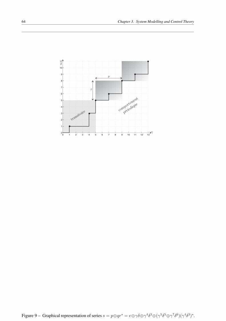
64 Chapter 3. System Modelling and Control Theory
Figure 9 – Graphical representation of series s = p�qr⇤ = e�����4�3�(�5�5��7�6)(�4�3)⇤.
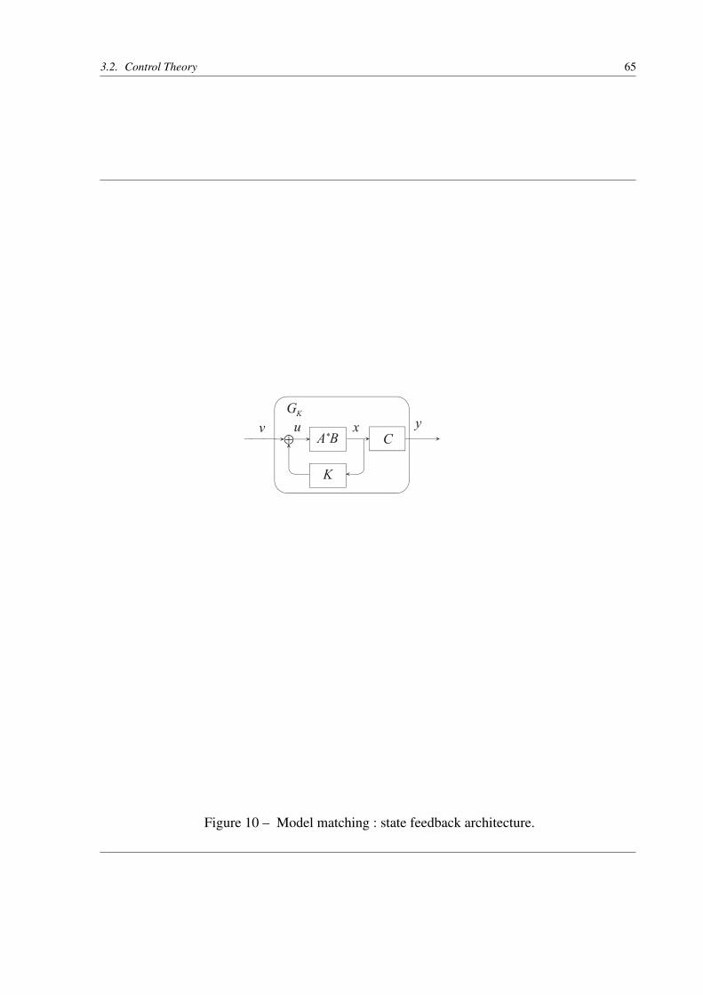
3.2. Control Theory 65
Figure 10 – Model matching : state feedback architecture.
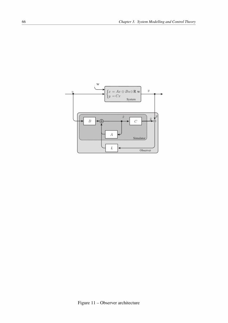
66 Chapter 3. System Modelling and Control Theory
Figure 11 – Observer architecture

3.2. Control Theory 67
Figure 12 – Control architecture using the estimated state

68 Chapter 3. System Modelling and Control Theory
Figure 13 – The Observer-based Controller
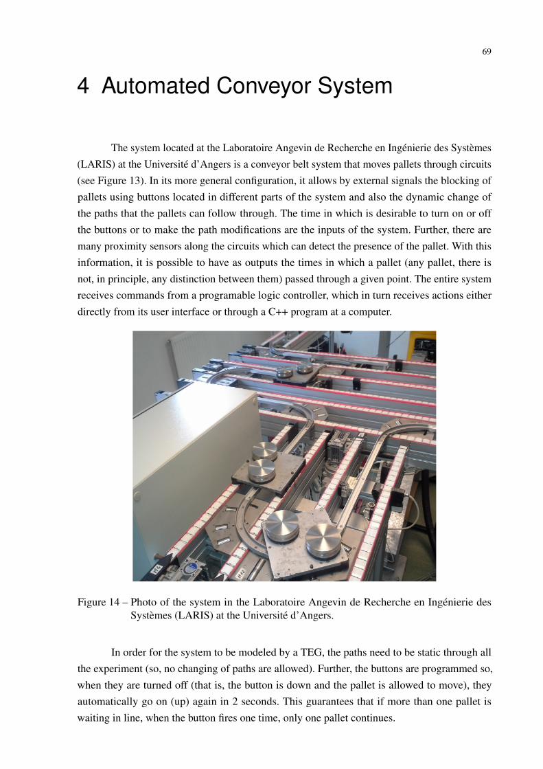
69
4 Automated Conveyor System
The system located at the Laboratoire Angevin de Recherche en Ingénierie des Systèmes(LARIS) at the Université d’Angers is a conveyor belt system that moves pallets through circuits(see Figure 13). In its more general configuration, it allows by external signals the blocking ofpallets using buttons located in different parts of the system and also the dynamic change ofthe paths that the pallets can follow through. The time in which is desirable to turn on or offthe buttons or to make the path modifications are the inputs of the system. Further, there aremany proximity sensors along the circuits which can detect the presence of the pallet. With thisinformation, it is possible to have as outputs the times in which a pallet (any pallet, there isnot, in principle, any distinction between them) passed through a given point. The entire systemreceives commands from a programable logic controller, which in turn receives actions eitherdirectly from its user interface or through a C++ program at a computer.
Figure 14 – Photo of the system in the Laboratoire Angevin de Recherche en Ingénierie desSystèmes (LARIS) at the Université d’Angers.
In order for the system to be modeled by a TEG, the paths need to be static through allthe experiment (so, no changing of paths are allowed). Further, the buttons are programmed so,when they are turned off (that is, the button is down and the pallet is allowed to move), theyautomatically go on (up) again in 2 seconds. This guarantees that if more than one pallet iswaiting in line, when the button fires one time, only one pallet continues.
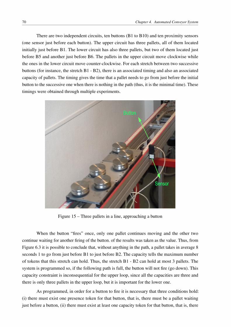
70 Chapter 4. Automated Conveyor System
There are two independent circuits, ten buttons (B1 to B10) and ten proximity sensors(one sensor just before each button). The upper circuit has three pallets, all of them locatedinitially just before B1. The lower circuit has also three pallets, but two of them located justbefore B5 and another just before B6. The pallets in the upper circuit move clockwise whilethe ones in the lower circuit move counter-clockwise. For each stretch between two successivebuttons (for instance, the stretch B1 - B2), there is an associated timing and also an associatedcapacity of pallets. The timing gives the time that a pallet needs to go from just before the initialbutton to the successive one when there is nothing in the path (thus, it is the minimal time). Thesetimings were obtained through multiple experiments.
Figure 15 – Three pallets in a line, approaching a button
When the button “fires” once, only one pallet continues moving and the other twocontinue waiting for another firing of the button. of the results was taken as the value. Thus, fromFigure 6.3 it is possible to conclude that, without anything in the path, a pallet takes in average 8seconds 1 to go from just before B1 to just before B2. The capacity tells the maximum numberof tokens that this stretch can hold. Thus, the stretch B1 - B2 can hold at most 3 pallets. Thesystem is programmed so, if the following path is full, the button will not fire (go down). Thiscapacity constraint is inconsequential for the upper loop, since all the capacities are three andthere is only three pallets in the upper loop, but it is important for the lower one.
As programmed, in order for a button to fire it is necessary that three conditions hold:(i) there must exist one presence token for that button, that is, there must be a pallet waitingjust before a button, (ii) there must exist at least one capacity token for that button, that is, there
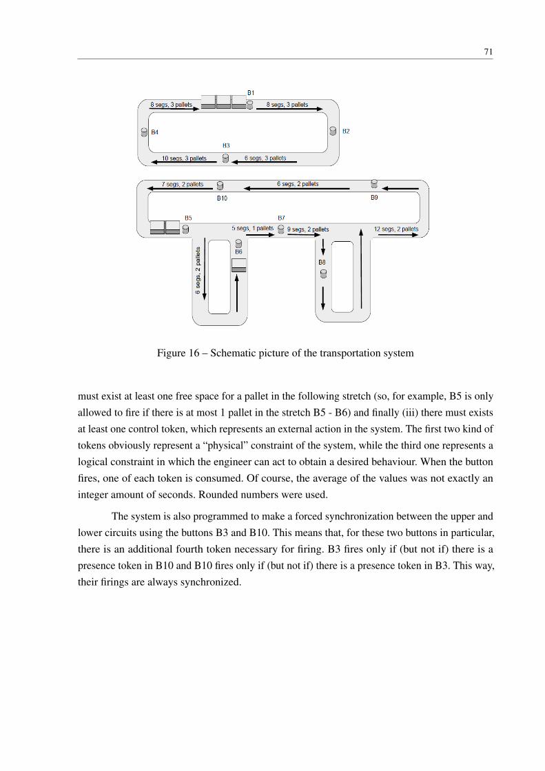
71
Figure 16 – Schematic picture of the transportation system
must exist at least one free space for a pallet in the following stretch (so, for example, B5 is onlyallowed to fire if there is at most 1 pallet in the stretch B5 - B6) and finally (iii) there must existsat least one control token, which represents an external action in the system. The first two kind oftokens obviously represent a “physical” constraint of the system, while the third one represents alogical constraint in which the engineer can act to obtain a desired behaviour. When the buttonfires, one of each token is consumed. Of course, the average of the values was not exactly aninteger amount of seconds. Rounded numbers were used.
The system is also programmed to make a forced synchronization between the upper andlower circuits using the buttons B3 and B10. This means that, for these two buttons in particular,there is an additional fourth token necessary for firing. B3 fires only if (but not if) there is apresence token in B10 and B10 fires only if (but not if) there is a presence token in B3. This way,their firings are always synchronized.

72 Chapter 4. Automated Conveyor System
4.1 System Description
A TEG model for this system is proposed in [21], by Dr. Vinícius Mariano Gonçalves.Before continuing, it is important to define the inputs u[k] and outputs y[k] of the system. Hence,it will be defined as ui[k], i = 1, 2, ..., 10 the time in which the kth control token is available forthe ith button. Further, yi[k], i = 1, 2, ...,10 the time in which the kth palled arrived just before theith button. Note that these definitions comply with what one can act and observe in the system.The modelling begins by analyzing each stretch. Suppose, to begin with, stretch B1 - B2. Forthis stretch, which holds three pallets at most, one can think in three possible status for a pallet(respective of one place in a TEG):(i) - P1: Stopped, in the first place in line before B2;(ii) - P2: Stopped, in the second place in line before B2;(iii) - P3: Stopped, in the third place in line before B2;Also, one needs four actions (respective of one transition in a TEG), labeled as x1, x2, x3 and x4:(i) - x1: Button B1 fired, began moving to B2;(ii) - x2: Began moving from the third place to the second place in line;(iii) - x3: Began moving from the second place to the first place in line;(iv) - x4: Button B2 fired, began moving to B3.
Note that:(i) - x1 can only fire if there is at least one capacity token (that is, a free space for a pallet) in thestretch B1 - B2, there is a presence token in the previous place (there is one, initially, see Figure6.3) and at least one control token is available. Further, at every firing of x4, one capacity tokenis restored to the stretch because one pallet is leaving. Since the stretch begins free of pallets(see Figure 2.3), initially there are three capacity tokens;(ii) - A pallet can only begin to move from the third place in line to the second one if there areno pallets in the second place. Thus, there must not exist a token/pallet in P2. Further, only onetoken/pallet can be at P2 at a given time (because only one pallet can be at the second place) andevery time x3 fires the space becomes free to a new pallet to go to the second position;(iii) - A pallet can only begin to move from the second place in line to the first one if there areno pallets in the first place. Thus, there must not exist a token/pallet in P1. Further, only onetoken/pallet can be at P1 at a given time (because only one pallet can be at the first place) andevery time x4 fires the space becomes free to a new pallet to go to the first position;(iv) - Of course, x4 can only fire if there is at least one capacity token in the stretch B2! B3,which initially is devoid of pallets and thus B2 has initially three capacity tokens. Further, theremust exist a presence token in P1 and also at least one control token for B2.
A final concern is that P3 can only have one token/pallet at a given time. The aboveconstraints naturally ensure this, and thus there is no need to force it artificially. Indeed, suppose
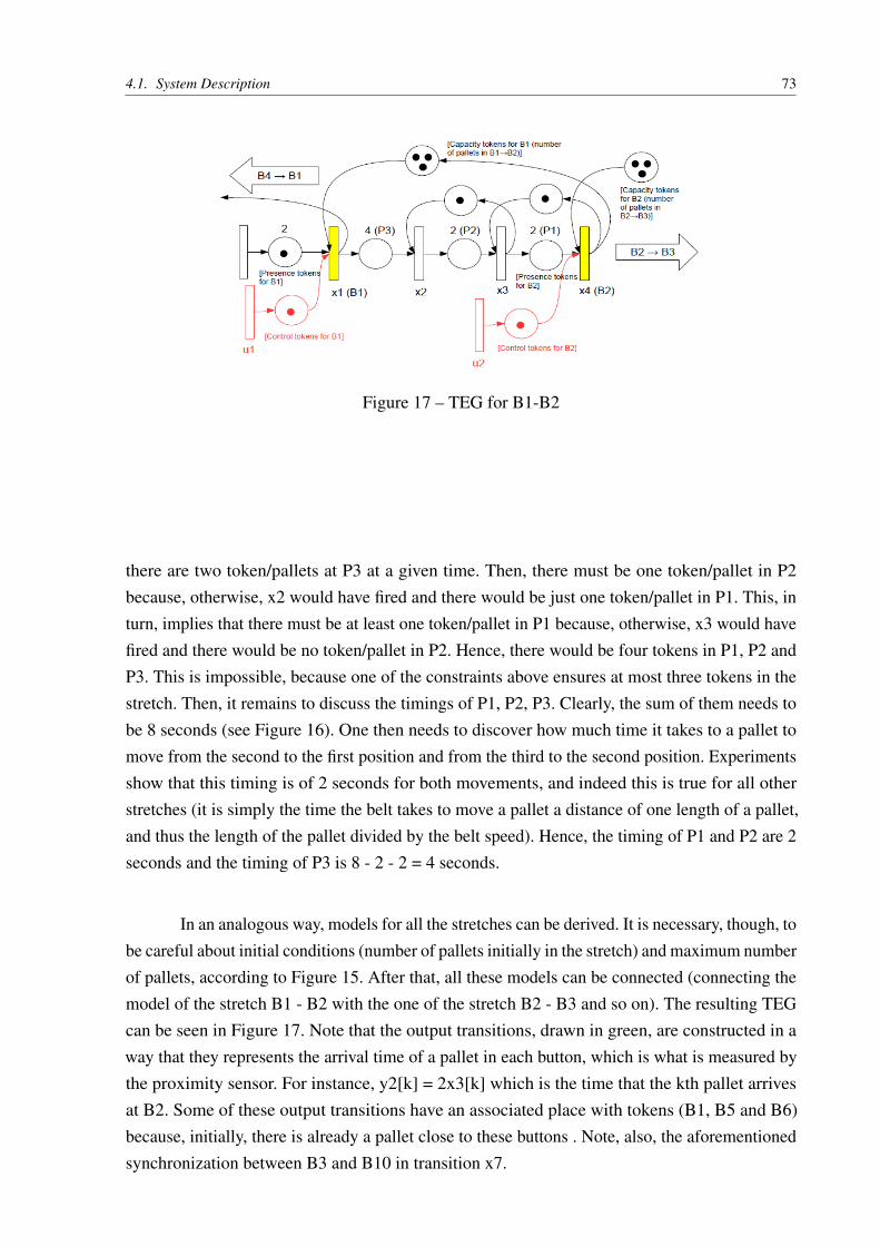
4.1. System Description 73
Figure 17 – TEG for B1-B2
there are two token/pallets at P3 at a given time. Then, there must be one token/pallet in P2because, otherwise, x2 would have fired and there would be just one token/pallet in P1. This, inturn, implies that there must be at least one token/pallet in P1 because, otherwise, x3 would havefired and there would be no token/pallet in P2. Hence, there would be four tokens in P1, P2 andP3. This is impossible, because one of the constraints above ensures at most three tokens in thestretch. Then, it remains to discuss the timings of P1, P2, P3. Clearly, the sum of them needs tobe 8 seconds (see Figure 16). One then needs to discover how much time it takes to a pallet tomove from the second to the first position and from the third to the second position. Experimentsshow that this timing is of 2 seconds for both movements, and indeed this is true for all otherstretches (it is simply the time the belt takes to move a pallet a distance of one length of a pallet,and thus the length of the pallet divided by the belt speed). Hence, the timing of P1 and P2 are 2seconds and the timing of P3 is 8 - 2 - 2 = 4 seconds.
In an analogous way, models for all the stretches can be derived. It is necessary, though, tobe careful about initial conditions (number of pallets initially in the stretch) and maximum numberof pallets, according to Figure 15. After that, all these models can be connected (connecting themodel of the stretch B1 - B2 with the one of the stretch B2 - B3 and so on). The resulting TEGcan be seen in Figure 17. Note that the output transitions, drawn in green, are constructed in away that they represents the arrival time of a pallet in each button, which is what is measured bythe proximity sensor. For instance, y2[k] = 2x3[k] which is the time that the kth pallet arrivesat B2. Some of these output transitions have an associated place with tokens (B1, B5 and B6)because, initially, there is already a pallet close to these buttons . Note, also, the aforementionedsynchronization between B3 and B10 in transition x7.

74 Chapter 4. Automated Conveyor System
4.2 System Modelling
For the TEG model presented in Figure 18, the system over the two-dimentional descrip-tion Max
in
[[�, �]], presented in last chapter 3.1.4, is described as the following:
State transition matrix A:
A =
" " " �
3" " " " " " " ��
2" " " " " " " " " "
�
4" � " " " " " " " " " " " " " " " " " " "
" �
2" � " " " " " " " " " " " " " " " " " "
" " �
2" " " �
3" " " " " " " " " " " " " " "
" " " �
2" � " " " " " " " " " " " " " " " "
" " " " �
2" � " " " " " " " " " " " " " " "
" " " " " �
2" " " �
3" " " e " " " " " " " �
2
" " " " " " �
6" � " " " " " " " " " " " " "
" " " " " " " �
2" � " " " " " " " " " " " "
e " " " " " " " �
2" " " " " " " " " " " " "
" " " " " " " " " ��
4" e " " " " " " " " " "
e " " " " " " " " " ��
2" " " " " " " " " " "
" " " " " " ��
5" " " " " " e " " " " " " " "
" " " " " " " " " " " " ��
2" " � " " " " " "
" " " " " " " " " " " " " �
4" e " " " " " "
" " " " " " " " " " " " " " ��
2" � " " " " "
" " " " " " " " " " " " " " " �
5" " �
2" " "
" " " " " " " " " " " " " " " " �
7" � " " "
" " " " " " " " " " " " " " " " " �
2" " �
2"
" " " " " " " " " " " " " " " " " " �
10" � "
" " " " " " �
2" " " " " " " " " " " " �
2" "
" " " " " " � " " " " " " " " " " " " " �
4"
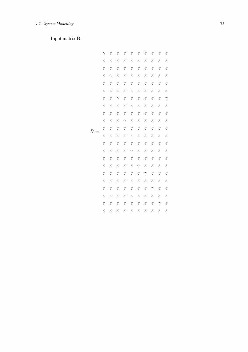
4.2. System Modelling 75
Input matrix B:
B =
� " " " " " " " " "
" " " " " " " " " "
" " " " " " " " " "
" � " " " " " " " "
" " " " " " " " " "
" " " " " " " " " "
" " � " " " " " " �
" " " " " " " " " "
" " " " " " " " " "
" " " � " " " " " "
" " " " " " " " " "
" " " " " " " " " "
" " " " " " " " " "
" " " " � " " " " "
" " " " " " " " " "
" " " " " � " " " "
" " " " " " � " " "
" " " " " " " " " "
" " " " " " " � " "
" " " " " " " " " "
" " " " " " " " � "
" " " " " " " " " "

76 Chapter 4. Automated Conveyor System
Output matrix C:
C =
" " " " " " " " " " " ��2 " " " " " " " " " "
" " �2 " " " " " " " " " " " " " " " " " " "
" " " " " �2 " " " " " " " " " " " " " " " "
" " " " " " " " �2 " " " " " " " " " " " " "
" " " " " " " " " " " " ��2 " " " " " " " " "
" " " " " " " " " " " " " " ��2 " " " " " " "
" " " " " " " " " " " " " " " �5 " " " " " "
" " " " " " " " " " " " " " " " " �2 " " " "
" " " " " " " " " " " " " " " " " " " �2 " "
" " " " " " " " " " " " " " " " " " " " " �2
The transfer function H = CA?B can be seen in Appendix A.
4.3 Control System
In this section the modified observer-based controller will be used to compute the state-feedback control law, which was described in the last chapter, section 3.2.3 .
For this problem the reference model Gref
will be defined as Gref
= H , it means thatthe controller aims to preserve the input/output performances of the system while increasing asmuch as possible the controlled input. The controlled system will be able to retard all controlentries, without losing performance.
All calculated controllers (M,P,Q and K) can be seen in Appendix A.
4.3.1 Time domain representation of u
As seen in section 3.2.3, equation 3.55, the control law u depends of the output y and thereference v. The automated conveyor system has 10 control inputs, in order to demonstrate theprocedure of convertion to time domain, the control input u
0
was chosen.
u0
= u0
y
+ u0
v
u0
= Qv �Ky
The control law, given in the time domain for u0
y
(t), can be represented using the (min-plus)-algebra as follows:
⇠00
(t), ⇠01
(t), ..., ⇠19
(t) are intermediated transactions introduced by our controller.

4.3. Control System 77
⇠00
(t) = 3⇠00
(t� 45)� 5y0
(t� 75)� 6y0
(t� 80)� 7y0
(t� 87)
⇠01
(t) = 3⇠01
(t� 45)� 5y1
(t� 67)� 6y1
(t� 72)� 7y1
(t� 79)
⇠02
(t) = 3⇠02
(t� 45)� 5y2
(t� 63)� 6y2
(t� 68)� 7y2
(t� 75)
⇠03
(t) = 3⇠03
(t� 45)� 8y3
(t� 83)� 9y3
(t� 88)� 10y3
(t� 95)
⇠04
(t) = 3⇠04
(t� 45)� 3y4
(t� 56)� 4y4
(t� 61)� 5y4
(t� 68)
⇠05
(t) = 3⇠05
(t� 45)� 2y5
(t� 50)� 3y5
(t� 55)� 4y5
(t� 62)
⇠06
(t) = 3⇠06
(t� 45)� 2y6
(t� 45)� 3y6
(t� 50)� 4y6
(t� 57)
⇠07
(t) = 3⇠07
(t� 45)� 4y7
(t� 48)� 5y7
(t� 81)� 6y7
(t� 86)
⇠08
(t) = 3⇠08
(t� 45)� 4y8
(t� 36)� 5y8
(t� 69)� 6y8
(t� 74)
⇠09
(t) = 3⇠09
(t� 45)� 5y9
(t� 68)� 6y9
(t� 68)� 7y9
(t� 75)
⇠0y
(t) = ⇠00
(t)� ⇠01
(t)� ...� ⇠08
(t)� ⇠09
(t)
u0
y
(t) = y0
(t� 2)� 1y0
(t� 4)� 2y0
(t� 30)� 3y0
(t� 34)� 4y0
(t� 2)� 2y1
(t� 22)�3y
1
(t� 26)� 4y1
(t� 30)� 2y2
(t� 18)� 3y2
(t� 222)� 4y2
(t� 26)� 3y3
(t� 8)� 3y3
(t�10)� 4y
3
(t� 12)� 5y3
(t� 38)� 6y3
(t� 42)� 7y3
(t� 46)� 2y4
(t� 18)� 2y7
(t� 36)�3y
7
(t� 40)� 2y8
(t� 24)� 3y8
(t� 28)� 2y9
(t� 18)� 3y9
(t� 22)� 4y9
(t� 26)� ⇠0y
(t)
The control law, given in the time domain for u0
v
(t), can be represented using the(min-plus)-algebra as follows:
⇠10
(t) = 3⇠10
(t� 45)� 6v0
(t� 75)� 7v0
(t� 80)� 5v0
(t� 87)
⇠11
(t) = 3⇠11
(t� 45)� 7v1
(t� 69)� 8v1
(t� 74)� 9v1
(t� 81)
⇠12
(t) = 3⇠12
(t� 45)� 6v2
(t� 63)� 7v2
(t� 68)� 8v2
(t� 75)
⇠13
(t) = 3⇠13
(t� 45)� 9v3
(t� 83)� 10v3
(t� 88)� 11v3
(t� 95)
⇠14
(t) = 3⇠14
(t� 45)� 4v4
(t� 56)� 5v4
(t� 61)� 6v4
(t� 95)
⇠15
(t) = 3⇠15
(t� 45)� 3v5
(t� 50)� 4v5
(t� 55)� 5v5
(t� 62)
⇠16
(t) = 3⇠16
(t� 45)� 3v6
(t� 45)� 4v6
(t� 50)� 5v6
(t� 57)
⇠17
(t) = 3⇠17
(t� 45)� 5v7
(t� 48)� 6v7
(t� 81)� 7v7
(t� 86)
⇠18
(t) = 3⇠18
(t� 45)� 5v8
(t� 36)� 6v8
(t� 69)� 7v8
(t� 74)
⇠19
(t) = 3⇠19
(t� 45)� 6v9
(t� 63)� 7v9
(t� 68)� 8v9
(t� 75)
⇠0v
(t) = ⇠10
(t)� ⇠11
(t)� ...� ⇠18
(t)� ⇠19
(t)
u0
v
(t) = v0
(t)� v0
(t� 2)� 2v0
(t� 4)� 3v0
(t� 30)� 4v0
(t� 34)� 5v0
(t� 38)� 3v1
(t)�

78 Chapter 4. Automated Conveyor System
4v1
(t�24)�5v1
(t�28)�6v1
(t�32)�3v2
(t�18)�3v2
(t�22)�5v2
(t�26)�3v3
(t�8)�4v
3
(t� 10)� 5v3
(t� 12)� 6v3
(t� 38)� 7v3
(t� 42)� 8v3
(t� 46)� 3v4
(t� 18)� 3v7
(t�36)�4v
7
(t�40)�3v8
(t�24)�4v3
(t�28)�3v9
(t�18)�4v9
(t�22)�5v9
(t�26)� ⇠0v
(t)
So, using the matrices Q and K previously defined, we can simplify and easily calculatethe control law u in time-domain, using the reference v and the output y. Now, its not necessaryto calculate the estimated state x to obtain the control law u.
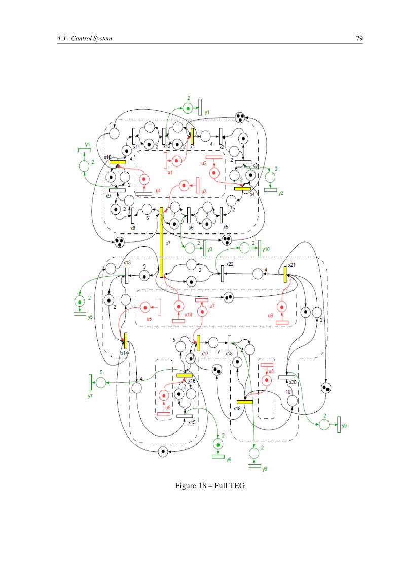
4.3. Control System 79
Figure 18 – Full TEG

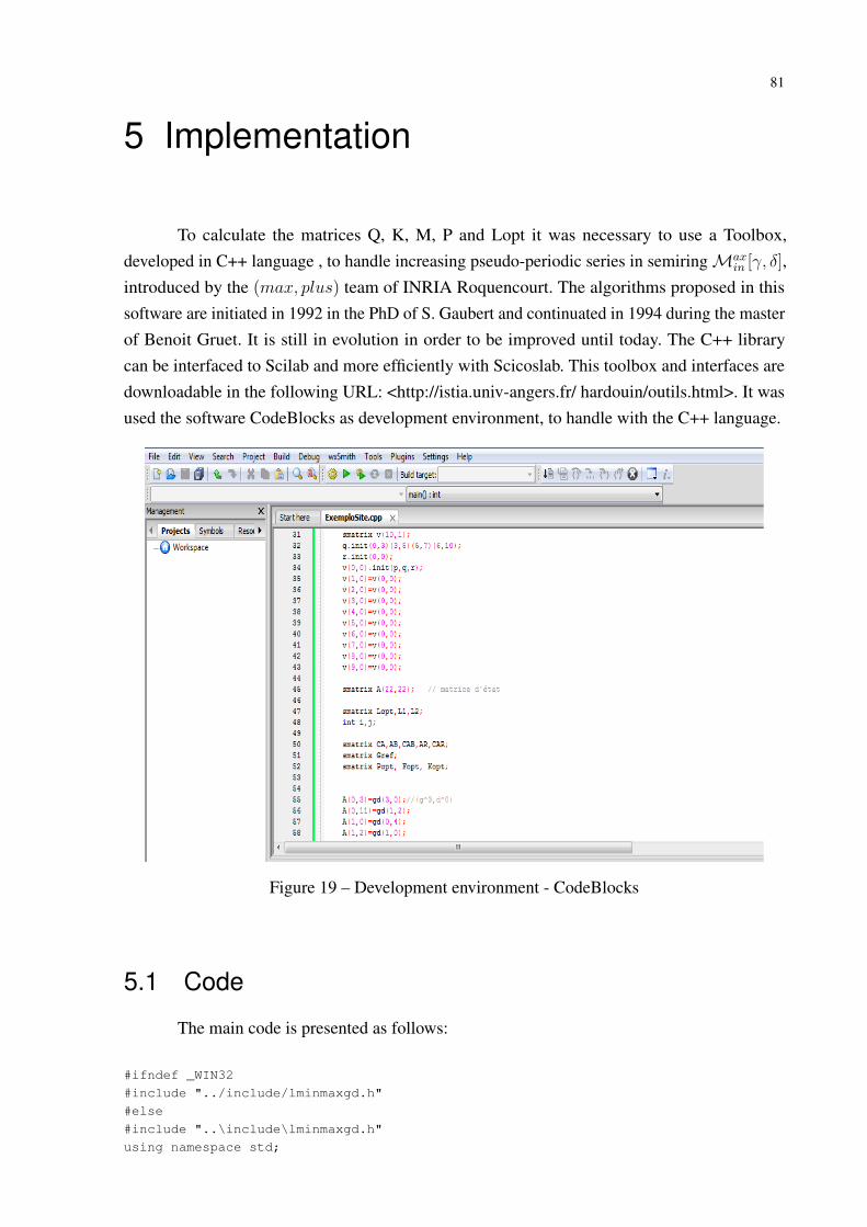
81
5 Implementation
To calculate the matrices Q, K, M, P and Lopt it was necessary to use a Toolbox,developed in C++ language , to handle increasing pseudo-periodic series in semiring Max
in
[�, �],introduced by the (max, plus) team of INRIA Roquencourt. The algorithms proposed in thissoftware are initiated in 1992 in the PhD of S. Gaubert and continuated in 1994 during the masterof Benoit Gruet. It is still in evolution in order to be improved until today. The C++ librarycan be interfaced to Scilab and more efficiently with Scicoslab. This toolbox and interfaces aredownloadable in the following URL: <http://istia.univ-angers.fr/ hardouin/outils.html>. It wasused the software CodeBlocks as development environment, to handle with the C++ language.
Figure 19 – Development environment - CodeBlocks
5.1 Code
The main code is presented as follows:
#ifndef _WIN32#include "../include/lminmaxgd.h"#else#include "..\include\lminmaxgd.h"using namespace std;

82 Chapter 5. Implementation
#endif
#include "..\src\gd.cpp"#include "..\src\poly.cpp"#include "..\src\serie.cpp"#include "..\src\smatrix.cpp"#include "..\src\tools.cpp"
At first it was necessary to include some C++ libraries in order to work with formalseries, monomials, polynomials and to compute the star of a matrix. From now, will be shownhow to calculate all controllers, the transfer matrix H and how to proceed a simulation using thetoolbox.
///////
int main() // Main Function{try{poly p,q;gd r;smatrix v(10,1);q.init(0,3)(3,5)(5,7)(6,10);r.init(0,0);v(0,0).init(p,q,r); // Reference vv(1,0)=v(0,0);v(2,0)=v(0,0);v(3,0)=v(0,0);v(4,0)=v(0,0);v(5,0)=v(0,0);v(6,0)=v(0,0);v(7,0)=v(0,0);v(8,0)=v(0,0);v(9,0)=v(0,0);
The reference v was defined using a polynomial, all entries have the same form, withoutlosing generality.
smatrix A(22,22); // Matrix A
smatrix Lopt,L1,L2;int i,j;
smatrix CA,AB,CAB,AR,CAR;smatrix Gref;smatrix Popt, Fopt, M;
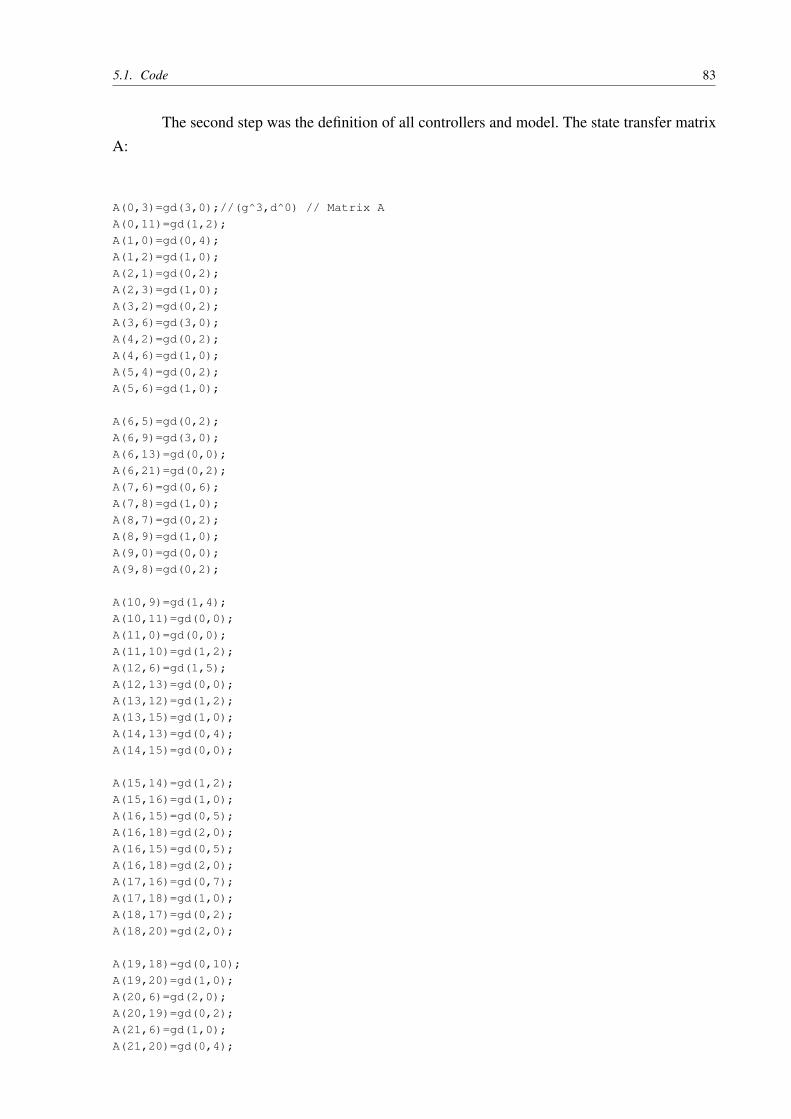
5.1. Code 83
The second step was the definition of all controllers and model. The state transfer matrixA:
A(0,3)=gd(3,0);//(g^3,d^0) // Matrix AA(0,11)=gd(1,2);A(1,0)=gd(0,4);A(1,2)=gd(1,0);A(2,1)=gd(0,2);A(2,3)=gd(1,0);A(3,2)=gd(0,2);A(3,6)=gd(3,0);A(4,2)=gd(0,2);A(4,6)=gd(1,0);A(5,4)=gd(0,2);A(5,6)=gd(1,0);
A(6,5)=gd(0,2);A(6,9)=gd(3,0);A(6,13)=gd(0,0);A(6,21)=gd(0,2);A(7,6)=gd(0,6);A(7,8)=gd(1,0);A(8,7)=gd(0,2);A(8,9)=gd(1,0);A(9,0)=gd(0,0);A(9,8)=gd(0,2);
A(10,9)=gd(1,4);A(10,11)=gd(0,0);A(11,0)=gd(0,0);A(11,10)=gd(1,2);A(12,6)=gd(1,5);A(12,13)=gd(0,0);A(13,12)=gd(1,2);A(13,15)=gd(1,0);A(14,13)=gd(0,4);A(14,15)=gd(0,0);
A(15,14)=gd(1,2);A(15,16)=gd(1,0);A(16,15)=gd(0,5);A(16,18)=gd(2,0);A(16,15)=gd(0,5);A(16,18)=gd(2,0);A(17,16)=gd(0,7);A(17,18)=gd(1,0);A(18,17)=gd(0,2);A(18,20)=gd(2,0);
A(19,18)=gd(0,10);A(19,20)=gd(1,0);A(20,6)=gd(2,0);A(20,19)=gd(0,2);A(21,6)=gd(1,0);A(21,20)=gd(0,4);

84 Chapter 5. Implementation
The output matrix C and input matrix B:
smatrix C(10,22); // Output Matrix CC(0,11)=gd(1,2);C(1,2)=gd(0,2);C(2,5)=gd(0,2);C(3,8)=gd(0,2);C(4,12)=gd(1,2);C(5,14)=gd(1,2);C(6,15)=gd(0,5);C(7,17)=gd(0,2);C(8,19)=gd(0,2);C(9,21)=gd(0,2);
smatrix B(22,10); // Matrix BB(0,0)=gd(1,0);B(3,1)=gd(1,0);B(6,2)=gd(1,0);B(6,9)=gd(1,0);B(9,3)=gd(1,0);B(13,4)=gd(1,0);B(15,5)=gd(1,0);B(16,6)=gd(1,0);B(18,7)=gd(1,0);B(20,8)=gd(1,0);
Matrix R represents the connections between the uncontrollable inputs and the statematrix. In our case R is defined as identity and we will not work with system disturbances.
smatrix R(22,22); // Matrix R = IdentityR(0,0)=gd(0,0);R(1,1)=gd(0,0);R(2,2)=gd(0,0);R(3,3)=gd(0,0);R(4,4)=gd(0,0);R(5,5)=gd(0,0);R(6,6)=gd(0,0);R(7,7)=gd(0,0);R(8,8)=gd(0,0);R(9,9)=gd(0,0);R(10,10)=gd(0,0);R(11,11)=gd(0,0);R(12,12)=gd(0,0);R(13,13)=gd(0,0);R(14,14)=gd(0,0);R(15,15)=gd(0,0);R(16,16)=gd(0,0);R(17,17)=gd(0,0);

5.1. Code 85
R(18,18)=gd(0,0);R(19,19)=gd(0,0);R(20,20)=gd(0,0);R(21,21)=gd(0,0);
Calculation of the Observer Lopt
smatrix As=star(A); // A*CA=otimes(C,As); // CA*
AB=otimes(As,B);CAB=otimes(C,AB);AR=otimes(As,R);CAR=otimes(C,AR);
L1=rfrac(AB,CAB);L2=rfrac(AR,CAR);Lopt=inf(L1,L2);Lopt=prcaus(Lopt); // Observer L_opt
fstream f;f.open("/Users/Matheus/Documents/libminmaxgd/examples/Lopt.txt",ios::out);f<<Lopt;f.close();
The desired behavior Gref
was defined equal to the transfer function Gref
= H = CA?B.Controllers M and P
opt
are also calculated. It is important to mention that as we are workingwith a real system, the use of causal controllers is required.
Gref=CAB; // Desired behavior Gref = CA*B =H
Popt=lfrac(Gref,CAB);M=otimes(AB,Popt);M=rfrac(Popt,M);M=lfrac(M,Popt);M=prcaus(M); // Causal M
Fopt=rfrac(M,C);Fopt=prcaus(Fopt); // Causal Fopt
fstream g;g.open("/Users/Matheus/Documents/libminmaxgd/examples/Fopt.txt",ios::out);g<<Fopt;g.close();
fstream h;
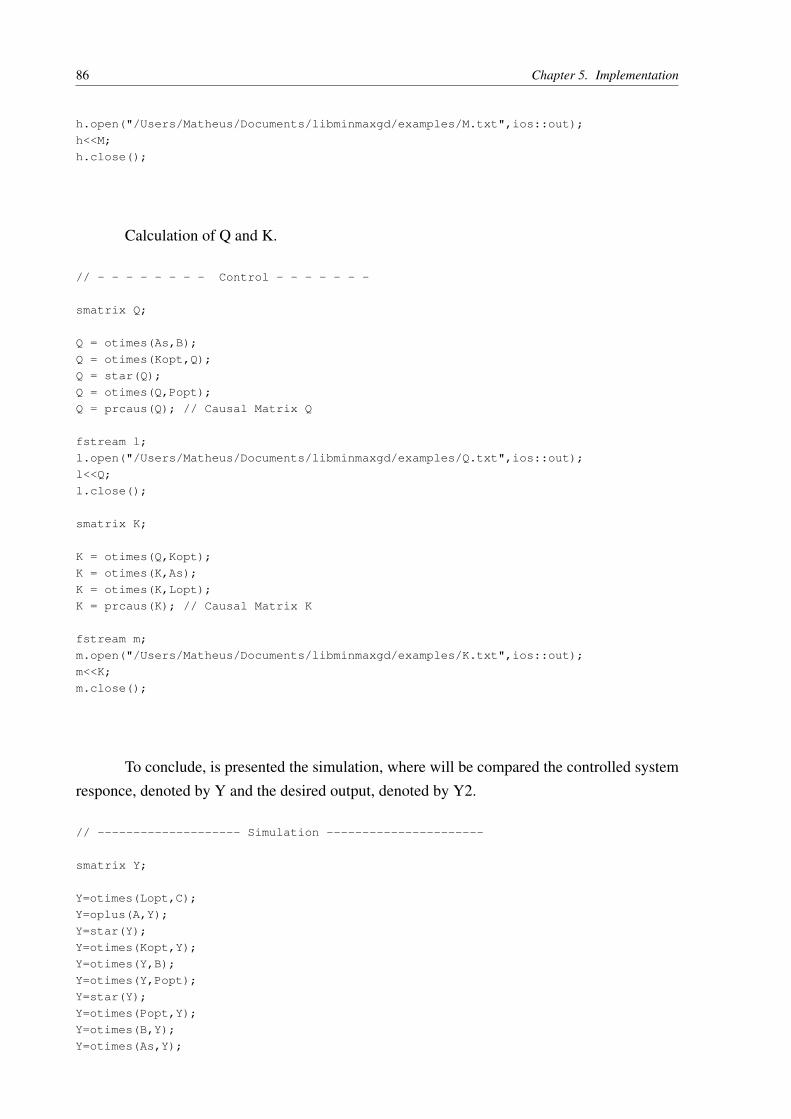
86 Chapter 5. Implementation
h.open("/Users/Matheus/Documents/libminmaxgd/examples/M.txt",ios::out);h<<M;h.close();
Calculation of Q and K.
// - - - - - - - - Control - - - - - - -
smatrix Q;
Q = otimes(As,B);Q = otimes(Kopt,Q);Q = star(Q);Q = otimes(Q,Popt);Q = prcaus(Q); // Causal Matrix Q
fstream l;l.open("/Users/Matheus/Documents/libminmaxgd/examples/Q.txt",ios::out);l<<Q;l.close();
smatrix K;
K = otimes(Q,Kopt);K = otimes(K,As);K = otimes(K,Lopt);K = prcaus(K); // Causal Matrix K
fstream m;m.open("/Users/Matheus/Documents/libminmaxgd/examples/K.txt",ios::out);m<<K;m.close();
To conclude, is presented the simulation, where will be compared the controlled systemresponce, denoted by Y and the desired output, denoted by Y2.
// -------------------- Simulation ----------------------
smatrix Y;
Y=otimes(Lopt,C);Y=oplus(A,Y);Y=star(Y);Y=otimes(Kopt,Y);Y=otimes(Y,B);Y=otimes(Y,Popt);Y=star(Y);Y=otimes(Popt,Y);Y=otimes(B,Y);Y=otimes(As,Y);
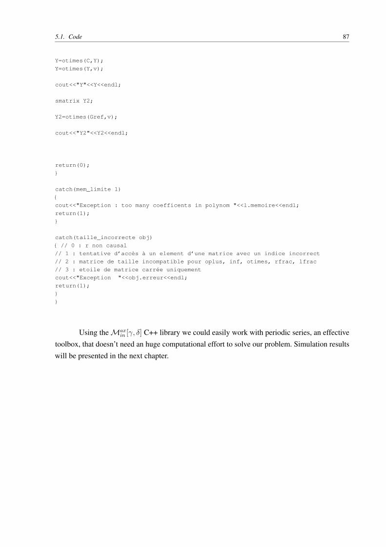
5.1. Code 87
Y=otimes(C,Y);Y=otimes(Y,v);
cout<<"Y"<<Y<<endl;
smatrix Y2;
Y2=otimes(Gref,v);
cout<<"Y2"<<Y2<<endl;
return(0);}
catch(mem_limite l){cout<<"Exception : too many coefficents in polynom "<<l.memoire<<endl;return(1);}
catch(taille_incorrecte obj){ // 0 : r non causal// 1 : tentative d’accès à un element d’une matrice avec un indice incorrect// 2 : matrice de taille incompatible pour oplus, inf, otimes, rfrac, lfrac// 3 : etoile de matrice carrée uniquementcout<<"Exception "<<obj.erreur<<endl;return(1);}}
Using the Max
in
[�, �] C++ library we could easily work with periodic series, an effectivetoolbox, that doesn’t need an huge computational effort to solve our problem. Simulation resultswill be presented in the next chapter.


89
6 Results
In order to test the efficacy of the observer-based controller a simulation was developed.Remembering, the objective is to get the greatest control law such that the output y be smallerthan or equal to the desired output G
ref
v.The desired behavior of the system Gref
, was definedequal to the transfer function H , which means G
ref
= H = CA?B.
It was performed a simple comparison between the controlled system responce, denotedby Y and the desired output, denoted by Y2.
Y = Cx = CA⇤BP (M(A� Lopt
C)
⇤BP )
⇤v (6.1)
Y 2 = Gref
v = Hv (6.2)
The following code represents how to calculate Y and Y2 using the Toolbox, developedin C++ language , to handle increasing pseudo-periodic series in semiring Max
in
[�, �], introducedby the (max, plus) team of INRIA Roquencourt.
----------------------------------- Simulation ----------------------------------smatrix Y;
Y=otimes(Lopt,C);Y=oplus(A,Y);Y=star(Y);Y=otimes(Kopt,Y);Y=otimes(Y,B);Y=otimes(Y,Popt);Y=star(Y);Y=otimes(Popt,Y);Y=otimes(B,Y);Y=otimes(As,Y);Y=otimes(C,Y);Y=otimes(Y,v);
cout<<"Y"<<Y<<endl;
smatrix Y2;
Y2=otimes(Gref,v);
cout<<"Y2"<<Y2<<endl;---------------------------------------------------------------------------------
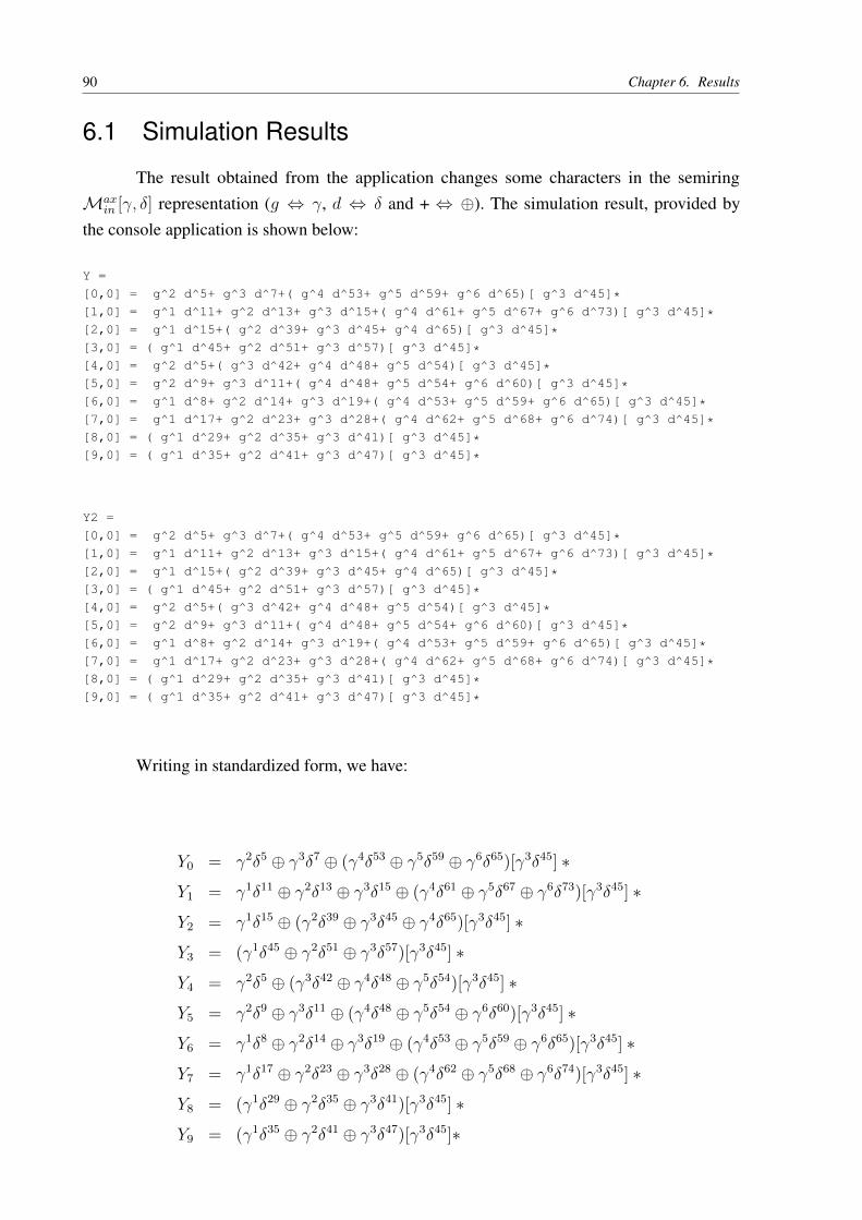
90 Chapter 6. Results
6.1 Simulation Results
The result obtained from the application changes some characters in the semiringMax
in
[�, �] representation (g , �, d , � and + , �). The simulation result, provided bythe console application is shown below:
Y =[0,0] = g^2 d^5+ g^3 d^7+( g^4 d^53+ g^5 d^59+ g^6 d^65)[ g^3 d^45]*[1,0] = g^1 d^11+ g^2 d^13+ g^3 d^15+( g^4 d^61+ g^5 d^67+ g^6 d^73)[ g^3 d^45]*[2,0] = g^1 d^15+( g^2 d^39+ g^3 d^45+ g^4 d^65)[ g^3 d^45]*[3,0] = ( g^1 d^45+ g^2 d^51+ g^3 d^57)[ g^3 d^45]*[4,0] = g^2 d^5+( g^3 d^42+ g^4 d^48+ g^5 d^54)[ g^3 d^45]*[5,0] = g^2 d^9+ g^3 d^11+( g^4 d^48+ g^5 d^54+ g^6 d^60)[ g^3 d^45]*[6,0] = g^1 d^8+ g^2 d^14+ g^3 d^19+( g^4 d^53+ g^5 d^59+ g^6 d^65)[ g^3 d^45]*[7,0] = g^1 d^17+ g^2 d^23+ g^3 d^28+( g^4 d^62+ g^5 d^68+ g^6 d^74)[ g^3 d^45]*[8,0] = ( g^1 d^29+ g^2 d^35+ g^3 d^41)[ g^3 d^45]*[9,0] = ( g^1 d^35+ g^2 d^41+ g^3 d^47)[ g^3 d^45]*
Y2 =[0,0] = g^2 d^5+ g^3 d^7+( g^4 d^53+ g^5 d^59+ g^6 d^65)[ g^3 d^45]*[1,0] = g^1 d^11+ g^2 d^13+ g^3 d^15+( g^4 d^61+ g^5 d^67+ g^6 d^73)[ g^3 d^45]*[2,0] = g^1 d^15+( g^2 d^39+ g^3 d^45+ g^4 d^65)[ g^3 d^45]*[3,0] = ( g^1 d^45+ g^2 d^51+ g^3 d^57)[ g^3 d^45]*[4,0] = g^2 d^5+( g^3 d^42+ g^4 d^48+ g^5 d^54)[ g^3 d^45]*[5,0] = g^2 d^9+ g^3 d^11+( g^4 d^48+ g^5 d^54+ g^6 d^60)[ g^3 d^45]*[6,0] = g^1 d^8+ g^2 d^14+ g^3 d^19+( g^4 d^53+ g^5 d^59+ g^6 d^65)[ g^3 d^45]*[7,0] = g^1 d^17+ g^2 d^23+ g^3 d^28+( g^4 d^62+ g^5 d^68+ g^6 d^74)[ g^3 d^45]*[8,0] = ( g^1 d^29+ g^2 d^35+ g^3 d^41)[ g^3 d^45]*[9,0] = ( g^1 d^35+ g^2 d^41+ g^3 d^47)[ g^3 d^45]*
Writing in standardized form, we have:
Y0
= �2�5 � �3�7 � (�4�53 � �5�59 � �6�65)[�3�45] ⇤
Y1
= �1�11 � �2�13 � �3�15 � (�4�61 � �5�67 � �6�73)[�3�45] ⇤
Y2
= �1�15 � (�2�39 � �3�45 � �4�65)[�3�45] ⇤
Y3
= (�1�45 � �2�51 � �3�57)[�3�45] ⇤
Y4
= �2�5 � (�3�42 � �4�48 � �5�54)[�3�45] ⇤
Y5
= �2�9 � �3�11 � (�4�48 � �5�54 � �6�60)[�3�45] ⇤
Y6
= �1�8 � �2�14 � �3�19 � (�4�53 � �5�59 � �6�65)[�3�45] ⇤
Y7
= �1�17 � �2�23 � �3�28 � (�4�62 � �5�68 � �6�74)[�3�45] ⇤
Y8
= (�1�29 � �2�35 � �3�41)[�3�45] ⇤
Y9
= (�1�35 � �2�41 � �3�47)[�3�45]⇤
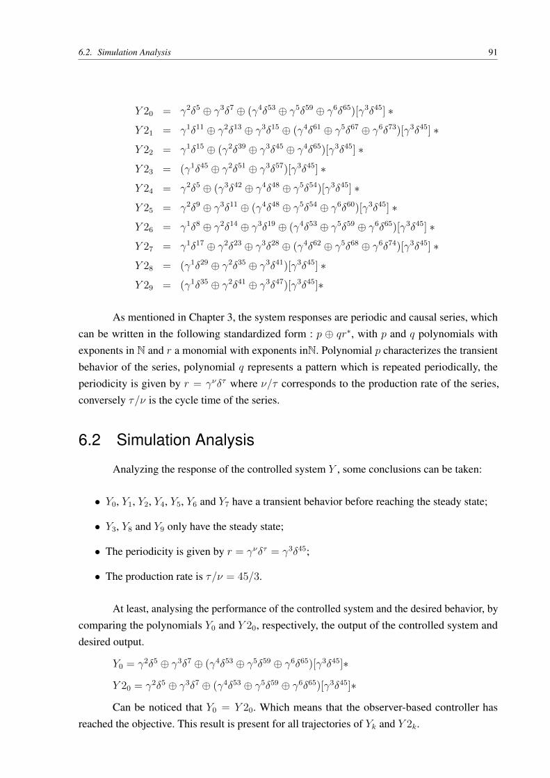
6.2. Simulation Analysis 91
Y 2
0
= �2�5 � �3�7 � (�4�53 � �5�59 � �6�65)[�3�45] ⇤
Y 2
1
= �1�11 � �2�13 � �3�15 � (�4�61 � �5�67 � �6�73)[�3�45] ⇤
Y 2
2
= �1�15 � (�2�39 � �3�45 � �4�65)[�3�45] ⇤
Y 2
3
= (�1�45 � �2�51 � �3�57)[�3�45] ⇤
Y 2
4
= �2�5 � (�3�42 � �4�48 � �5�54)[�3�45] ⇤
Y 2
5
= �2�9 � �3�11 � (�4�48 � �5�54 � �6�60)[�3�45] ⇤
Y 2
6
= �1�8 � �2�14 � �3�19 � (�4�53 � �5�59 � �6�65)[�3�45] ⇤
Y 2
7
= �1�17 � �2�23 � �3�28 � (�4�62 � �5�68 � �6�74)[�3�45] ⇤
Y 2
8
= (�1�29 � �2�35 � �3�41)[�3�45] ⇤
Y 2
9
= (�1�35 � �2�41 � �3�47)[�3�45]⇤
As mentioned in Chapter 3, the system responses are periodic and causal series, whichcan be written in the following standardized form : p � qr⇤, with p and q polynomials withexponents in N and r a monomial with exponents inN. Polynomial p characterizes the transientbehavior of the series, polynomial q represents a pattern which is repeated periodically, theperiodicity is given by r = �⌫�⌧ where ⌫/⌧ corresponds to the production rate of the series,conversely ⌧/⌫ is the cycle time of the series.
6.2 Simulation Analysis
Analyzing the response of the controlled system Y , some conclusions can be taken:
• Y0
, Y1
, Y2
, Y4
, Y5
, Y6
and Y7
have a transient behavior before reaching the steady state;
• Y3
, Y8
and Y9
only have the steady state;
• The periodicity is given by r = �⌫�⌧ = �3�45;
• The production rate is ⌧/⌫ = 45/3.
At least, analysing the performance of the controlled system and the desired behavior, bycomparing the polynomials Y
0
and Y 2
0
, respectively, the output of the controlled system anddesired output.
Y0
= �2�5 � �3�7 � (�4�53 � �5�59 � �6�65)[�3�45]⇤
Y 2
0
= �2�5 � �3�7 � (�4�53 � �5�59 � �6�65)[�3�45]⇤
Can be noticed that Y0
= Y 2
0
. Which means that the observer-based controller hasreached the objective. This result is present for all trajectories of Y
k
and Y 2
k
.

93
7 Conclusion
The first general objective of the project - to develop a model for the automated conveyorsystem located in LARIS using a TEG model proposed by Dr. Vinícius Mariano Gonçalves inhis thesis [21] and the two-dimentional description Max
in
[[�, �]] for (Max,+) linear systems, wasachieved.
Using the Observer-based Controller for (Max,+) linear systems, based on the workintroduced by Prof. Laurent Hardouin in [22] , the second general objective of the project was tocontrol the automated conveyor system. Some algebraic manipulations were proposed by me,in order to simplify the way of obtaining the control law u in the time domain. Now, it is notnecessary to calculate the u using the estimated state x. The control law can be calculated basedon the reference input v and the output of the system Y .
To calculate the observer-based controller it was necessary to use a Toolbox, developedin C++ language , to handle with increasing pseudo-periodic series in semiring Max
in
[�, �],introduced by the (max, plus) team of INRIA Roquencourt.
After the calculation of the controllers, a simulation of the controlled system has beenproposed. The output of the controlled system Y was compared with the desired output Y 2 =
Gref
v. As we can observe in Chapter 6 specification has been reached. Therefore, the controlledsystem has the same performance of the reference system G
ref
, but their controlled inputs u aredelayed as much as possible. For just-in-time problems this is a very important result.
As a possible continuation of this work, uncertain TEG models can be used to representpossible modelling errors.

95
Bibliography
1 HARDOUIN, L. et al. L’algèbre (max,+) pour l’ingénieur. sur la commande des systèmes(max,+) linéaires. 2009. Citado na página 19.
2 BLYTH, T. Lattices and Ordered Algebraic Structures. [S.l.]: Springer, 2005. Citado 2 vezesnas páginas 21 and 34.
3 DAVEY, B.; PRIESTLEY, H. Introduction to Lattices and Order. [S.l.]: CambridgeUniversity Press, 1990. Citado 2 vezes nas páginas 21 and 33.
4 BLYTH, T.; JANOWITZ, M. Residuation Theory. [S.l.]: Pergamon press, 1972. Citado 5vezes nas páginas 21, 33, 36, 37, and 38.
5 BACCELLI, F. et al. Synchronization and Linearity : An Algebra for Discrete Event Systems.[S.l.]: Wiley and Sons, 1992. Citado 10 vezes nas páginas 21, 25, 26, 29, 30, 32, 34, 35, 37,and 51.
6 GAUBERT, S. Théorie des Systèmes Linéaires dans les Dioïdes. Tese (Thèse) — École desMines de Paris, July 1992. Nenhuma citação no texto.
7 COTTENCEAU, B. Contribution à la commande de systèmes à événements discrets :synthèse de correcteurs pour les graphes d’événements temporisés dans les dioïdes. Tese (Thèse)— LISA - Université d’Angers, 1999. Citado 2 vezes nas páginas 34 and 38.
8 COHEN, G. Residuation and applications. Algèbres Max-Plus et applications en informatiqueet automatique, Ecole de printemps d’informatique théorique, Noirmoutier, 1998. Citado 3vezes nas páginas 34, 36, and 37.
9 LHOMMEAU, M. Étude de systèmes à événements discrets dans l’algèbre (max,+). 1.Synthèse de correcteurs robustes dans un dioïde d’intervalles. 2. Synthèse de correcteurs enprésence de perturbations. Tese (Doutorado) — ISTIA – Université d’Angers, Angers, France,dez. 2003. Citado 2 vezes nas páginas 34 and 37.
10 OUERGHI, I. Etude et commande de systèmes (max,+)-linéaires soumis à des contraintes.In: PhD, Universit’e d’Angers. Angers, France: [s.n.], 2006. Advisor : L. Hardouin. Citado napágina 34.
11 COHEN, G.; GAUBERT, S.; QUADRAT, J.-P. Linear projectors in the max-plus algebra. In:Proceedings of the IEEE-Mediterranean Conference. Cyprus: [s.n.], 1997. Citado na página 36.
12 MENGUY, E. Contribution à la commande des systèmes linéaires dans les dioïdes. Tese(Thèse) — LISA - Université d’Angers, 1997. Citado na página 37.
13 LHOMMEAU, M. et al. Interval Analysis and Dioid: Application to Robust ControllerDesign for Timed Event Graphs. Automatica, v. 40, n. 11, p. 1923–1930, nov. 2004. Available at<doi:10.1016/j.automatica.2004.05.013>. Citado na página 38.
14 COTTENCEAU, B. et al. Model Reference Control for Timed Event Graphsin Dioids. Automatica, v. 37, n. 9, p. 1451–1458, set. 2001. Available at <doi:10.1016/S0005-1098(01)00073-5>. Citado 2 vezes nas páginas 38 and 56.

96 Bibliography
15 COHEN, G.; GAUBERT, S.; QUADRAT, J.-P. Kernels, images and projections in dioids. In:Proceedings of WODES’96. Edinburgh: [s.n.], 1996. Citado na página 39.
16 COHEN, G. et al. A linear system theoretic view of discrete event processes and its usefor performance evaluation in manufacturing. IEEE Trans. on Automatic Control, AC–30, p.210–220, 1985. Citado 2 vezes nas páginas 43 and 44.
17 COHEN, G.; GAUBERT, S.; QUADRAT, J.-P. Algebraic system analysis of timed Petrinets. In: GUNAWARDENA, J. (Ed.). Idempotency. [S.l.]: Cambridge University Press, 1995,(Publications of the Newton Institute). To appear in 1996. Citado na página 44.
18 COHEN, G. Théorie algébrique des systèmes à événements discrets. [S.l.]: Polycopié decours donné à l’INRIA, 1995. Citado na página 49.
19 COHEN, G. Two-dimensional domain representation of timed event graphs. In: SummerSchool on Discrete Event Systems. [S.l.]: Spa, Belgium, 1993. Citado na página 51.
20 LUENBERGER, D. An introduction to observers. IEEE Trans. on Automatic Control, v. 16,n. 6, p. 596–602, 1971. Citado na página 57.
21 GONçALVES, V. M. TROPICAL ALGORITHMS FOR LINEAR ALGEBRA AND LINEAREVENT-INVARIANT DYNAMICAL SYSTEMS. Tese (Thèse) — Universidade Federal de MinasGerais, UFMG, Brazil, 2014. Citado 3 vezes nas páginas 19, 72, and 93.
22 L. Hardouin et al. Extended version with source code of the paper observer=basedcontrollers for max-plus linear systems. 2015. Citado 3 vezes nas páginas 61, 62, and 93.

Appendix

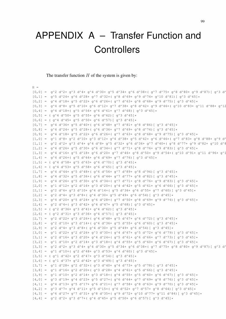
99
APPENDIX A – Transfer Function andControllers
The transfer function H of the system is given by:
H =[0,0] = g^2 d^2+ g^3 d^4+ g^4 d^30+ g^5 d^34+ g^6 d^38+( g^7 d^75+ g^8 d^80+ g^9 d^87)[ g^3 d^45]*[0,1] = g^5 d^24+ g^6 d^28+ g^7 d^32+( g^8 d^69+ g^9 d^74+ g^10 d^81)[ g^3 d^45]*[0,2] = g^4 d^18+ g^5 d^22+ g^6 d^26+( g^7 d^63+ g^8 d^68+ g^9 d^75)[ g^3 d^45]*[0,3] = g^4 d^8+ g^5 d^10+ g^6 d^12+ g^7 d^38+ g^8 d^42+ g^9 d^46+( g^10 d^83+ g^11 d^88+ g^12 d^95)[ g^3 d^45]*[0,4] = g^4 d^18+( g^5 d^56+ g^6 d^61+ g^7 d^68)[ g^3 d^45]*[0,5] = ( g^4 d^50+ g^5 d^55+ g^6 d^62)[ g^3 d^45]*[0,6] = ( g^4 d^45+ g^5 d^50+ g^6 d^57)[ g^3 d^45]*[0,7] = g^4 d^36+ g^5 d^40+( g^6 d^48+ g^7 d^81+ g^8 d^86)[ g^3 d^45]*[0,8] = g^4 d^24+ g^5 d^28+( g^6 d^36+ g^7 d^69+ g^8 d^74)[ g^3 d^45]*[0,9] = g^4 d^18+ g^5 d^22+ g^6 d^26+( g^7 d^63+ g^8 d^68+ g^9 d^75)[ g^3 d^45]*[1,0] = g^1 d^8+ g^2 d^10+ g^3 d^12+ g^4 d^38+ g^5 d^42+ g^6 d^46+( g^7 d^83+ g^8 d^88+ g^9 d^95)[ g^3 d^45]*[1,1] = g^2 d^2+ g^3 d^4+ g^4 d^8+ g^5 d^32+ g^6 d^36+ g^7 d^40+( g^8 d^77+ g^9 d^82+ g^10 d^89)[ g^3 d^45]*[1,2] = g^4 d^26+ g^5 d^30+ g^6 d^34+( g^7 d^71+ g^8 d^76+ g^9 d^83)[ g^3 d^45]*[1,3] = g^4 d^16+ g^5 d^18+ g^6 d^20+ g^7 d^46+ g^8 d^50+ g^9 d^54+( g^10 d^91+ g^11 d^96+ g^12 d^103)[ g^3 d^45]*[1,4] = g^4 d^26+( g^5 d^64+ g^6 d^69+ g^7 d^76)[ g^3 d^45]*[1,5] = ( g^4 d^58+ g^5 d^63+ g^6 d^70)[ g^3 d^45]*[1,6] = ( g^4 d^53+ g^5 d^58+ g^6 d^65)[ g^3 d^45]*[1,7] = g^4 d^44+ g^5 d^48+( g^6 d^56+ g^7 d^89+ g^8 d^94)[ g^3 d^45]*[1,8] = g^4 d^32+ g^5 d^36+( g^6 d^44+ g^7 d^77+ g^8 d^82)[ g^3 d^45]*[1,9] = g^4 d^26+ g^5 d^30+ g^6 d^34+( g^7 d^71+ g^8 d^76+ g^9 d^83)[ g^3 d^45]*[2,0] = g^1 d^12+ g^2 d^16+ g^3 d^20+( g^4 d^42+ g^5 d^61+ g^6 d^66)[ g^3 d^45]*[2,1] = g^2 d^6+ g^3 d^10+ g^4 d^14+( g^5 d^36+ g^6 d^55+ g^7 d^60)[ g^3 d^45]*[2,2] = g^2 d^4+ g^3 d^8+( g^4 d^30+ g^5 d^49+ g^6 d^54)[ g^3 d^45]*[2,3] = g^4 d^20+ g^5 d^24+ g^6 d^28+( g^7 d^50+ g^8 d^69+ g^9 d^74)[ g^3 d^45]*[2,4] = g^2 d^4+( g^3 d^42+ g^4 d^47+ g^5 d^68)[ g^3 d^45]*[2,5] = ( g^2 d^36+ g^3 d^41+ g^4 d^62)[ g^3 d^45]*[2,6] = ( g^2 d^31+ g^3 d^36+ g^4 d^57)[ g^3 d^45]*[2,7] = g^2 d^22+ g^3 d^26+( g^4 d^48+ g^5 d^67+ g^6 d^72)[ g^3 d^45]*[2,8] = g^2 d^10+ g^3 d^14+( g^4 d^36+ g^5 d^55+ g^6 d^60)[ g^3 d^45]*[2,9] = g^2 d^4+ g^3 d^8+( g^4 d^30+ g^5 d^49+ g^6 d^54)[ g^3 d^45]*[3,0] = g^1 d^22+ g^2 d^26+ g^3 d^30+( g^4 d^67+ g^5 d^72+ g^6 d^79)[ g^3 d^45]*[3,1] = g^2 d^16+ g^3 d^20+ g^4 d^24+( g^5 d^61+ g^6 d^66+ g^7 d^73)[ g^3 d^45]*[3,2] = g^1 d^10+ g^2 d^14+ g^3 d^18+( g^4 d^55+ g^5 d^60+ g^6 d^67)[ g^3 d^45]*[3,3] = g^2 d^2+ g^3 d^4+ g^4 d^30+ g^5 d^34+ g^6 d^38+( g^7 d^75+ g^8 d^80+ g^9 d^87)[ g^3 d^45]*[3,4] = g^1 d^10+( g^2 d^48+ g^3 d^53+ g^4 d^60)[ g^3 d^45]*[3,5] = ( g^1 d^42+ g^2 d^47+ g^3 d^54)[ g^3 d^45]*[3,6] = ( g^1 d^37+ g^2 d^42+ g^3 d^49)[ g^3 d^45]*[3,7] = g^1 d^28+ g^2 d^32+( g^3 d^40+ g^4 d^73+ g^5 d^78)[ g^3 d^45]*[3,8] = g^1 d^16+ g^2 d^20+( g^3 d^28+ g^4 d^61+ g^5 d^66)[ g^3 d^45]*[3,9] = g^1 d^10+ g^2 d^14+ g^3 d^18+( g^4 d^55+ g^5 d^60+ g^6 d^67)[ g^3 d^45]*[4,0] = g^3 d^19+ g^4 d^23+ g^5 d^27+( g^6 d^64+ g^7 d^69+ g^8 d^76)[ g^3 d^45]*[4,1] = g^4 d^13+ g^5 d^17+ g^6 d^21+( g^7 d^58+ g^8 d^63+ g^9 d^70)[ g^3 d^45]*[4,2] = g^3 d^7+ g^4 d^11+ g^5 d^15+( g^6 d^52+ g^7 d^57+ g^8 d^64)[ g^3 d^45]*[4,3] = g^6 d^27+ g^7 d^31+ g^8 d^35+( g^9 d^72+ g^10 d^77+ g^11 d^84)[ g^3 d^45]*[4,4] = g^2 d^2+ g^3 d^7+( g^4 d^45+ g^5 d^50+ g^6 d^57)[ g^3 d^45]*

100 APPENDIX A. Transfer Function and Controllers
[4,5] = ( g^3 d^39+ g^4 d^44+ g^5 d^51)[ g^3 d^45]*[4,6] = ( g^3 d^34+ g^4 d^39+ g^5 d^46)[ g^3 d^45]*[4,7] = g^3 d^25+ g^4 d^29+( g^5 d^37+ g^6 d^70+ g^7 d^75)[ g^3 d^45]*[4,8] = g^3 d^13+ g^4 d^17+( g^5 d^25+ g^6 d^58+ g^7 d^63)[ g^3 d^45]*[4,9] = g^3 d^7+ g^4 d^11+ g^5 d^15+( g^6 d^52+ g^7 d^57+ g^8 d^64)[ g^3 d^45]*[5,0] = g^4 d^25+ g^5 d^29+ g^6 d^33+( g^7 d^70+ g^8 d^75+ g^9 d^82)[ g^3 d^45]*[5,1] = g^5 d^19+ g^6 d^23+ g^7 d^27+( g^8 d^64+ g^9 d^69+ g^10 d^76)[ g^3 d^45]*[5,2] = g^4 d^13+ g^5 d^17+ g^6 d^21+( g^7 d^58+ g^8 d^63+ g^9 d^70)[ g^3 d^45]*[5,3] = g^7 d^33+ g^8 d^37+ g^9 d^41+( g^10 d^78+ g^11 d^83+ g^12 d^90)[ g^3 d^45]*[5,4] = g^2 d^6+ g^3 d^8+ g^4 d^13+( g^5 d^51+ g^6 d^56+ g^7 d^63)[ g^3 d^45]*[5,5] = g^2 d^2+ g^3 d^7+( g^4 d^45+ g^5 d^50+ g^6 d^57)[ g^3 d^45]*[5,6] = g^3 d^2+( g^4 d^40+ g^5 d^45+ g^6 d^52)[ g^3 d^45]*[5,7] = g^4 d^31+ g^5 d^35+( g^6 d^43+ g^7 d^76+ g^8 d^81)[ g^3 d^45]*[5,8] = g^4 d^19+ g^5 d^23+( g^6 d^31+ g^7 d^64+ g^8 d^69)[ g^3 d^45]*[5,9] = g^4 d^13+ g^5 d^17+ g^6 d^21+( g^7 d^58+ g^8 d^63+ g^9 d^70)[ g^3 d^45]*[6,0] = g^4 d^30+ g^5 d^35+ g^6 d^40+( g^7 d^75+ g^8 d^80+ g^9 d^87)[ g^3 d^45]*[6,1] = g^5 d^24+ g^6 d^29+ g^7 d^34+( g^8 d^69+ g^9 d^74+ g^10 d^81)[ g^3 d^45]*[6,2] = g^4 d^18+ g^5 d^23+ g^6 d^28+( g^7 d^63+ g^8 d^68+ g^9 d^75)[ g^3 d^45]*[6,3] = g^7 d^38+ g^8 d^43+ g^9 d^48+( g^10 d^83+ g^11 d^88+ g^12 d^95)[ g^3 d^45]*[6,4] = g^2 d^11+ g^3 d^16+ g^4 d^21+( g^5 d^56+ g^6 d^61+ g^7 d^68)[ g^3 d^45]*[6,5] = g^1 d^5+ g^2 d^10+ g^3 d^15+( g^4 d^50+ g^5 d^55+ g^6 d^62)[ g^3 d^45]*[6,6] = g^2 d^5+ g^3 d^10+( g^4 d^45+ g^5 d^50+ g^6 d^57)[ g^3 d^45]*[6,7] = ( g^4 d^36+ g^5 d^41+ g^6 d^48)[ g^3 d^45]*[6,8] = ( g^4 d^24+ g^5 d^29+ g^6 d^36)[ g^3 d^45]*[6,9] = g^4 d^18+ g^5 d^23+ g^6 d^28+( g^7 d^63+ g^8 d^68+ g^9 d^75)[ g^3 d^45]*[7,0] = g^4 d^39+ g^5 d^44+ g^6 d^49+( g^7 d^84+ g^8 d^89+ g^9 d^96)[ g^3 d^45]*[7,1] = g^5 d^33+ g^6 d^38+ g^7 d^43+( g^8 d^78+ g^9 d^83+ g^10 d^90)[ g^3 d^45]*[7,2] = g^4 d^27+ g^5 d^32+ g^6 d^37+( g^7 d^72+ g^8 d^77+ g^9 d^84)[ g^3 d^45]*[7,3] = g^7 d^47+ g^8 d^52+ g^9 d^57+( g^10 d^92+ g^11 d^97+ g^12 d^104)[ g^3 d^45]*[7,4] = g^2 d^20+ g^3 d^25+ g^4 d^30+( g^5 d^65+ g^6 d^70+ g^7 d^77)[ g^3 d^45]*[7,5] = g^1 d^14+ g^2 d^19+ g^3 d^24+( g^4 d^59+ g^5 d^64+ g^6 d^71)[ g^3 d^45]*[7,6] = g^1 d^9+ g^2 d^14+ g^3 d^19+( g^4 d^54+ g^5 d^59+ g^6 d^66)[ g^3 d^45]*[7,7] = g^2 d^2+ g^3 d^9+( g^4 d^45+ g^5 d^50+ g^6 d^57)[ g^3 d^45]*[7,8] = ( g^4 d^33+ g^5 d^38+ g^6 d^45)[ g^3 d^45]*[7,9] = g^4 d^27+ g^5 d^32+ g^6 d^37+( g^7 d^72+ g^8 d^77+ g^9 d^84)[ g^3 d^45]*[8,0] = ( g^4 d^51+ g^5 d^56+ g^6 d^63)[ g^3 d^45]*[8,1] = ( g^5 d^45+ g^6 d^50+ g^7 d^57)[ g^3 d^45]*[8,2] = ( g^4 d^39+ g^5 d^44+ g^6 d^51)[ g^3 d^45]*[8,3] = ( g^7 d^59+ g^8 d^64+ g^9 d^71)[ g^3 d^45]*[8,4] = ( g^2 d^32+ g^3 d^37+ g^4 d^44)[ g^3 d^45]*[8,5] = ( g^1 d^26+ g^2 d^31+ g^3 d^38)[ g^3 d^45]*[8,6] = ( g^1 d^21+ g^2 d^26+ g^3 d^33)[ g^3 d^45]*[8,7] = g^1 d^12+ g^2 d^14+( g^3 d^24+ g^4 d^57+ g^5 d^62)[ g^3 d^45]*[8,8] = g^2 d^2+( g^3 d^12+ g^4 d^45+ g^5 d^50)[ g^3 d^45]*[8,9] = ( g^4 d^39+ g^5 d^44+ g^6 d^51)[ g^3 d^45]*[9,0] = g^2 d^14+ g^3 d^18+( g^4 d^57+ g^5 d^62+ g^6 d^69)[ g^3 d^45]*[9,1] = g^3 d^8+ g^4 d^12+( g^5 d^51+ g^6 d^56+ g^7 d^63)[ g^3 d^45]*[9,2] = g^2 d^2+ g^3 d^6+( g^4 d^45+ g^5 d^50+ g^6 d^57)[ g^3 d^45]*[9,3] = g^5 d^22+ g^6 d^26+( g^7 d^65+ g^8 d^70+ g^9 d^77)[ g^3 d^45]*[9,4] = ( g^2 d^38+ g^3 d^43+ g^4 d^50)[ g^3 d^45]*[9,5] = ( g^1 d^32+ g^2 d^37+ g^3 d^44)[ g^3 d^45]*[9,6] = ( g^1 d^27+ g^2 d^32+ g^3 d^39)[ g^3 d^45]*[9,7] = g^1 d^18+ g^2 d^20+( g^3 d^30+ g^4 d^63+ g^5 d^68)[ g^3 d^45]*[9,8] = g^1 d^6+ g^2 d^8+( g^3 d^18+ g^4 d^51+ g^5 d^56)[ g^3 d^45]*[9,9] = g^2 d^2+ g^3 d^6+( g^4 d^45+ g^5 d^50+ g^6 d^57)[ g^3 d^45]*
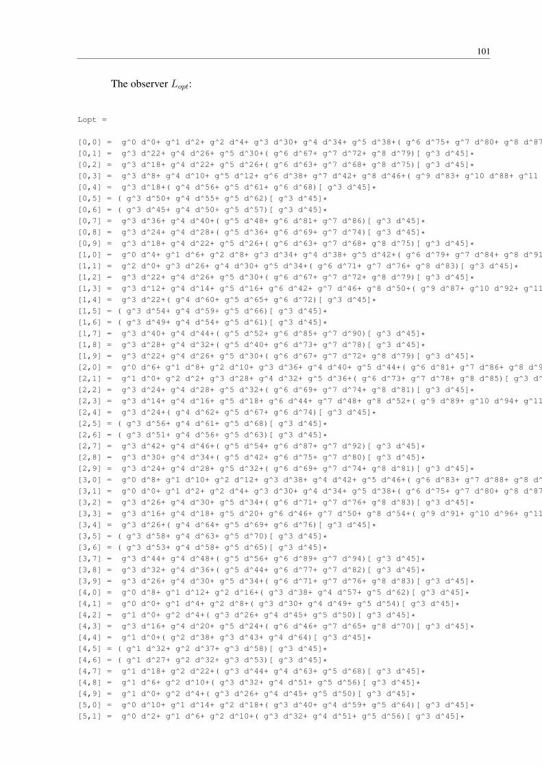
101
The observer Lopt
:
Lopt =
[0,0] = g^0 d^0+ g^1 d^2+ g^2 d^4+ g^3 d^30+ g^4 d^34+ g^5 d^38+( g^6 d^75+ g^7 d^80+ g^8 d^87)[ g^3 d^45]*[0,1] = g^3 d^22+ g^4 d^26+ g^5 d^30+( g^6 d^67+ g^7 d^72+ g^8 d^79)[ g^3 d^45]*[0,2] = g^3 d^18+ g^4 d^22+ g^5 d^26+( g^6 d^63+ g^7 d^68+ g^8 d^75)[ g^3 d^45]*[0,3] = g^3 d^8+ g^4 d^10+ g^5 d^12+ g^6 d^38+ g^7 d^42+ g^8 d^46+( g^9 d^83+ g^10 d^88+ g^11 d^95)[ g^3 d^45]*[0,4] = g^3 d^18+( g^4 d^56+ g^5 d^61+ g^6 d^68)[ g^3 d^45]*[0,5] = ( g^3 d^50+ g^4 d^55+ g^5 d^62)[ g^3 d^45]*[0,6] = ( g^3 d^45+ g^4 d^50+ g^5 d^57)[ g^3 d^45]*[0,7] = g^3 d^36+ g^4 d^40+( g^5 d^48+ g^6 d^81+ g^7 d^86)[ g^3 d^45]*[0,8] = g^3 d^24+ g^4 d^28+( g^5 d^36+ g^6 d^69+ g^7 d^74)[ g^3 d^45]*[0,9] = g^3 d^18+ g^4 d^22+ g^5 d^26+( g^6 d^63+ g^7 d^68+ g^8 d^75)[ g^3 d^45]*[1,0] = g^0 d^4+ g^1 d^6+ g^2 d^8+ g^3 d^34+ g^4 d^38+ g^5 d^42+( g^6 d^79+ g^7 d^84+ g^8 d^91)[ g^3 d^45]*[1,1] = g^2 d^0+ g^3 d^26+ g^4 d^30+ g^5 d^34+( g^6 d^71+ g^7 d^76+ g^8 d^83)[ g^3 d^45]*[1,2] = g^3 d^22+ g^4 d^26+ g^5 d^30+( g^6 d^67+ g^7 d^72+ g^8 d^79)[ g^3 d^45]*[1,3] = g^3 d^12+ g^4 d^14+ g^5 d^16+ g^6 d^42+ g^7 d^46+ g^8 d^50+( g^9 d^87+ g^10 d^92+ g^11 d^99)[ g^3 d^45]*[1,4] = g^3 d^22+( g^4 d^60+ g^5 d^65+ g^6 d^72)[ g^3 d^45]*[1,5] = ( g^3 d^54+ g^4 d^59+ g^5 d^66)[ g^3 d^45]*[1,6] = ( g^3 d^49+ g^4 d^54+ g^5 d^61)[ g^3 d^45]*[1,7] = g^3 d^40+ g^4 d^44+( g^5 d^52+ g^6 d^85+ g^7 d^90)[ g^3 d^45]*[1,8] = g^3 d^28+ g^4 d^32+( g^5 d^40+ g^6 d^73+ g^7 d^78)[ g^3 d^45]*[1,9] = g^3 d^22+ g^4 d^26+ g^5 d^30+( g^6 d^67+ g^7 d^72+ g^8 d^79)[ g^3 d^45]*[2,0] = g^0 d^6+ g^1 d^8+ g^2 d^10+ g^3 d^36+ g^4 d^40+ g^5 d^44+( g^6 d^81+ g^7 d^86+ g^8 d^93)[ g^3 d^45]*[2,1] = g^1 d^0+ g^2 d^2+ g^3 d^28+ g^4 d^32+ g^5 d^36+( g^6 d^73+ g^7 d^78+ g^8 d^85)[ g^3 d^45]*[2,2] = g^3 d^24+ g^4 d^28+ g^5 d^32+( g^6 d^69+ g^7 d^74+ g^8 d^81)[ g^3 d^45]*[2,3] = g^3 d^14+ g^4 d^16+ g^5 d^18+ g^6 d^44+ g^7 d^48+ g^8 d^52+( g^9 d^89+ g^10 d^94+ g^11 d^101)[ g^3 d^45]*[2,4] = g^3 d^24+( g^4 d^62+ g^5 d^67+ g^6 d^74)[ g^3 d^45]*[2,5] = ( g^3 d^56+ g^4 d^61+ g^5 d^68)[ g^3 d^45]*[2,6] = ( g^3 d^51+ g^4 d^56+ g^5 d^63)[ g^3 d^45]*[2,7] = g^3 d^42+ g^4 d^46+( g^5 d^54+ g^6 d^87+ g^7 d^92)[ g^3 d^45]*[2,8] = g^3 d^30+ g^4 d^34+( g^5 d^42+ g^6 d^75+ g^7 d^80)[ g^3 d^45]*[2,9] = g^3 d^24+ g^4 d^28+ g^5 d^32+( g^6 d^69+ g^7 d^74+ g^8 d^81)[ g^3 d^45]*[3,0] = g^0 d^8+ g^1 d^10+ g^2 d^12+ g^3 d^38+ g^4 d^42+ g^5 d^46+( g^6 d^83+ g^7 d^88+ g^8 d^95)[ g^3 d^45]*[3,1] = g^0 d^0+ g^1 d^2+ g^2 d^4+ g^3 d^30+ g^4 d^34+ g^5 d^38+( g^6 d^75+ g^7 d^80+ g^8 d^87)[ g^3 d^45]*[3,2] = g^3 d^26+ g^4 d^30+ g^5 d^34+( g^6 d^71+ g^7 d^76+ g^8 d^83)[ g^3 d^45]*[3,3] = g^3 d^16+ g^4 d^18+ g^5 d^20+ g^6 d^46+ g^7 d^50+ g^8 d^54+( g^9 d^91+ g^10 d^96+ g^11 d^103)[ g^3 d^45]*[3,4] = g^3 d^26+( g^4 d^64+ g^5 d^69+ g^6 d^76)[ g^3 d^45]*[3,5] = ( g^3 d^58+ g^4 d^63+ g^5 d^70)[ g^3 d^45]*[3,6] = ( g^3 d^53+ g^4 d^58+ g^5 d^65)[ g^3 d^45]*[3,7] = g^3 d^44+ g^4 d^48+( g^5 d^56+ g^6 d^89+ g^7 d^94)[ g^3 d^45]*[3,8] = g^3 d^32+ g^4 d^36+( g^5 d^44+ g^6 d^77+ g^7 d^82)[ g^3 d^45]*[3,9] = g^3 d^26+ g^4 d^30+ g^5 d^34+( g^6 d^71+ g^7 d^76+ g^8 d^83)[ g^3 d^45]*[4,0] = g^0 d^8+ g^1 d^12+ g^2 d^16+( g^3 d^38+ g^4 d^57+ g^5 d^62)[ g^3 d^45]*[4,1] = g^0 d^0+ g^1 d^4+ g^2 d^8+( g^3 d^30+ g^4 d^49+ g^5 d^54)[ g^3 d^45]*[4,2] = g^1 d^0+ g^2 d^4+( g^3 d^26+ g^4 d^45+ g^5 d^50)[ g^3 d^45]*[4,3] = g^3 d^16+ g^4 d^20+ g^5 d^24+( g^6 d^46+ g^7 d^65+ g^8 d^70)[ g^3 d^45]*[4,4] = g^1 d^0+( g^2 d^38+ g^3 d^43+ g^4 d^64)[ g^3 d^45]*[4,5] = ( g^1 d^32+ g^2 d^37+ g^3 d^58)[ g^3 d^45]*[4,6] = ( g^1 d^27+ g^2 d^32+ g^3 d^53)[ g^3 d^45]*[4,7] = g^1 d^18+ g^2 d^22+( g^3 d^44+ g^4 d^63+ g^5 d^68)[ g^3 d^45]*[4,8] = g^1 d^6+ g^2 d^10+( g^3 d^32+ g^4 d^51+ g^5 d^56)[ g^3 d^45]*[4,9] = g^1 d^0+ g^2 d^4+( g^3 d^26+ g^4 d^45+ g^5 d^50)[ g^3 d^45]*[5,0] = g^0 d^10+ g^1 d^14+ g^2 d^18+( g^3 d^40+ g^4 d^59+ g^5 d^64)[ g^3 d^45]*[5,1] = g^0 d^2+ g^1 d^6+ g^2 d^10+( g^3 d^32+ g^4 d^51+ g^5 d^56)[ g^3 d^45]*
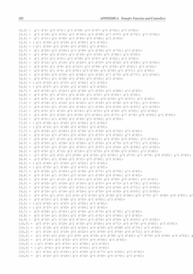
102 APPENDIX A. Transfer Function and Controllers
[5,2] = g^1 d^2+ g^2 d^6+( g^3 d^28+ g^4 d^47+ g^5 d^52)[ g^3 d^45]*[5,3] = g^3 d^18+ g^4 d^22+ g^5 d^26+( g^6 d^48+ g^7 d^67+ g^8 d^72)[ g^3 d^45]*[5,4] = g^1 d^2+( g^2 d^40+ g^3 d^45+ g^4 d^66)[ g^3 d^45]*[5,5] = ( g^1 d^34+ g^2 d^39+ g^3 d^60)[ g^3 d^45]*[5,6] = ( g^1 d^29+ g^2 d^34+ g^3 d^55)[ g^3 d^45]*[5,7] = g^1 d^20+ g^2 d^24+( g^3 d^46+ g^4 d^65+ g^5 d^70)[ g^3 d^45]*[5,8] = g^1 d^8+ g^2 d^12+( g^3 d^34+ g^4 d^53+ g^5 d^58)[ g^3 d^45]*[5,9] = g^1 d^2+ g^2 d^6+( g^3 d^28+ g^4 d^47+ g^5 d^52)[ g^3 d^45]*[6,0] = g^0 d^12+ g^1 d^16+ g^2 d^20+( g^3 d^57+ g^4 d^62+ g^5 d^69)[ g^3 d^45]*[6,1] = g^0 d^4+ g^1 d^8+ g^2 d^12+( g^3 d^49+ g^4 d^54+ g^5 d^61)[ g^3 d^45]*[6,2] = g^0 d^0+ g^1 d^4+ g^2 d^8+( g^3 d^45+ g^4 d^50+ g^5 d^57)[ g^3 d^45]*[6,3] = g^3 d^20+ g^4 d^24+ g^5 d^28+( g^6 d^65+ g^7 d^70+ g^8 d^77)[ g^3 d^45]*[6,4] = g^0 d^0+( g^1 d^38+ g^2 d^43+ g^3 d^50)[ g^3 d^45]*[6,5] = ( g^0 d^32+ g^1 d^37+ g^2 d^44)[ g^3 d^45]*[6,6] = ( g^0 d^27+ g^1 d^32+ g^2 d^39)[ g^3 d^45]*[6,7] = g^0 d^18+ g^1 d^22+( g^2 d^30+ g^3 d^63+ g^4 d^68)[ g^3 d^45]*[6,8] = g^0 d^6+ g^1 d^10+( g^2 d^18+ g^3 d^51+ g^4 d^56)[ g^3 d^45]*[6,9] = g^0 d^0+ g^1 d^4+ g^2 d^8+( g^3 d^45+ g^4 d^50+ g^5 d^57)[ g^3 d^45]*[7,0] = g^0 d^18+ g^1 d^22+ g^2 d^26+( g^3 d^63+ g^4 d^68+ g^5 d^75)[ g^3 d^45]*[7,1] = g^0 d^10+ g^1 d^14+ g^2 d^18+( g^3 d^55+ g^4 d^60+ g^5 d^67)[ g^3 d^45]*[7,2] = g^0 d^6+ g^1 d^10+ g^2 d^14+( g^3 d^51+ g^4 d^56+ g^5 d^63)[ g^3 d^45]*[7,3] = g^2 d^0+ g^3 d^26+ g^4 d^30+ g^5 d^34+( g^6 d^71+ g^7 d^76+ g^8 d^83)[ g^3 d^45]*[7,4] = g^0 d^6+( g^1 d^44+ g^2 d^49+ g^3 d^56)[ g^3 d^45]*[7,5] = ( g^0 d^38+ g^1 d^43+ g^2 d^50)[ g^3 d^45]*[7,6] = ( g^0 d^33+ g^1 d^38+ g^2 d^45)[ g^3 d^45]*[7,7] = g^0 d^24+ g^1 d^28+( g^2 d^36+ g^3 d^69+ g^4 d^74)[ g^3 d^45]*[7,8] = g^0 d^12+ g^1 d^16+( g^2 d^24+ g^3 d^57+ g^4 d^62)[ g^3 d^45]*[7,9] = g^0 d^6+ g^1 d^10+ g^2 d^14+( g^3 d^51+ g^4 d^56+ g^5 d^63)[ g^3 d^45]*[8,0] = g^0 d^20+ g^1 d^24+ g^2 d^28+( g^3 d^65+ g^4 d^70+ g^5 d^77)[ g^3 d^45]*[8,1] = g^0 d^12+ g^1 d^16+ g^2 d^20+( g^3 d^57+ g^4 d^62+ g^5 d^69)[ g^3 d^45]*[8,2] = g^0 d^8+ g^1 d^12+ g^2 d^16+( g^3 d^53+ g^4 d^58+ g^5 d^65)[ g^3 d^45]*[8,3] = g^1 d^0+ g^2 d^2+ g^3 d^28+ g^4 d^32+ g^5 d^36+( g^6 d^73+ g^7 d^78+ g^8 d^85)[ g^3 d^45]*[8,4] = g^0 d^8+( g^1 d^46+ g^2 d^51+ g^3 d^58)[ g^3 d^45]*[8,5] = ( g^0 d^40+ g^1 d^45+ g^2 d^52)[ g^3 d^45]*[8,6] = ( g^0 d^35+ g^1 d^40+ g^2 d^47)[ g^3 d^45]*[8,7] = g^0 d^26+ g^1 d^30+( g^2 d^38+ g^3 d^71+ g^4 d^76)[ g^3 d^45]*[8,8] = g^0 d^14+ g^1 d^18+( g^2 d^26+ g^3 d^59+ g^4 d^64)[ g^3 d^45]*[8,9] = g^0 d^8+ g^1 d^12+ g^2 d^16+( g^3 d^53+ g^4 d^58+ g^5 d^65)[ g^3 d^45]*[9,0] = g^0 d^22+ g^1 d^26+ g^2 d^30+( g^3 d^67+ g^4 d^72+ g^5 d^79)[ g^3 d^45]*[9,1] = g^0 d^14+ g^1 d^18+ g^2 d^22+( g^3 d^59+ g^4 d^64+ g^5 d^71)[ g^3 d^45]*[9,2] = g^0 d^10+ g^1 d^14+ g^2 d^18+( g^3 d^55+ g^4 d^60+ g^5 d^67)[ g^3 d^45]*[9,3] = g^0 d^0+ g^1 d^2+ g^2 d^4+ g^3 d^30+ g^4 d^34+ g^5 d^38+( g^6 d^75+ g^7 d^80+ g^8 d^87)[ g^3 d^45]*[9,4] = g^0 d^10+( g^1 d^48+ g^2 d^53+ g^3 d^60)[ g^3 d^45]*[9,5] = ( g^0 d^42+ g^1 d^47+ g^2 d^54)[ g^3 d^45]*[9,6] = ( g^0 d^37+ g^1 d^42+ g^2 d^49)[ g^3 d^45]*[9,7] = g^0 d^28+ g^1 d^32+( g^2 d^40+ g^3 d^73+ g^4 d^78)[ g^3 d^45]*[9,8] = g^0 d^16+ g^1 d^20+( g^2 d^28+ g^3 d^61+ g^4 d^66)[ g^3 d^45]*[9,9] = g^0 d^10+ g^1 d^14+ g^2 d^18+( g^3 d^55+ g^4 d^60+ g^5 d^67)[ g^3 d^45]*[10,0] = g^0 d^0+ g^1 d^26+ g^2 d^30+ g^3 d^34+( g^4 d^71+ g^5 d^76+ g^6 d^83)[ g^3 d^45]*[10,1] = g^1 d^18+ g^2 d^22+ g^3 d^26+( g^4 d^63+ g^5 d^68+ g^6 d^75)[ g^3 d^45]*[10,2] = g^1 d^14+ g^2 d^18+ g^3 d^22+( g^4 d^59+ g^5 d^64+ g^6 d^71)[ g^3 d^45]*[10,3] = g^1 d^4+ g^2 d^6+ g^3 d^8+ g^4 d^34+ g^5 d^38+ g^6 d^42+( g^7 d^79+ g^8 d^84+ g^9 d^91)[ g^3 d^45]*[10,4] = g^1 d^14+( g^2 d^52+ g^3 d^57+ g^4 d^64)[ g^3 d^45]*[10,5] = ( g^1 d^46+ g^2 d^51+ g^3 d^58)[ g^3 d^45]*[10,6] = ( g^1 d^41+ g^2 d^46+ g^3 d^53)[ g^3 d^45]*[10,7] = g^1 d^32+ g^2 d^36+( g^3 d^44+ g^4 d^77+ g^5 d^82)[ g^3 d^45]*[10,8] = g^1 d^20+ g^2 d^24+( g^3 d^32+ g^4 d^65+ g^5 d^70)[ g^3 d^45]*
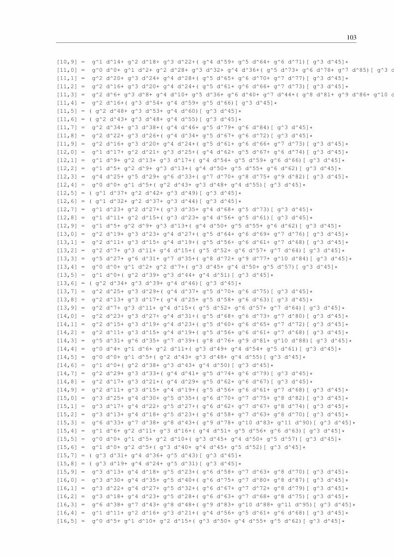
103
[10,9] = g^1 d^14+ g^2 d^18+ g^3 d^22+( g^4 d^59+ g^5 d^64+ g^6 d^71)[ g^3 d^45]*[11,0] = g^0 d^0+ g^1 d^2+ g^2 d^28+ g^3 d^32+ g^4 d^36+( g^5 d^73+ g^6 d^78+ g^7 d^85)[ g^3 d^45]*[11,1] = g^2 d^20+ g^3 d^24+ g^4 d^28+( g^5 d^65+ g^6 d^70+ g^7 d^77)[ g^3 d^45]*[11,2] = g^2 d^16+ g^3 d^20+ g^4 d^24+( g^5 d^61+ g^6 d^66+ g^7 d^73)[ g^3 d^45]*[11,3] = g^2 d^6+ g^3 d^8+ g^4 d^10+ g^5 d^36+ g^6 d^40+ g^7 d^44+( g^8 d^81+ g^9 d^86+ g^10 d^93)[ g^3 d^45]*[11,4] = g^2 d^16+( g^3 d^54+ g^4 d^59+ g^5 d^66)[ g^3 d^45]*[11,5] = ( g^2 d^48+ g^3 d^53+ g^4 d^60)[ g^3 d^45]*[11,6] = ( g^2 d^43+ g^3 d^48+ g^4 d^55)[ g^3 d^45]*[11,7] = g^2 d^34+ g^3 d^38+( g^4 d^46+ g^5 d^79+ g^6 d^84)[ g^3 d^45]*[11,8] = g^2 d^22+ g^3 d^26+( g^4 d^34+ g^5 d^67+ g^6 d^72)[ g^3 d^45]*[11,9] = g^2 d^16+ g^3 d^20+ g^4 d^24+( g^5 d^61+ g^6 d^66+ g^7 d^73)[ g^3 d^45]*[12,0] = g^1 d^17+ g^2 d^21+ g^3 d^25+( g^4 d^62+ g^5 d^67+ g^6 d^74)[ g^3 d^45]*[12,1] = g^1 d^9+ g^2 d^13+ g^3 d^17+( g^4 d^54+ g^5 d^59+ g^6 d^66)[ g^3 d^45]*[12,2] = g^1 d^5+ g^2 d^9+ g^3 d^13+( g^4 d^50+ g^5 d^55+ g^6 d^62)[ g^3 d^45]*[12,3] = g^4 d^25+ g^5 d^29+ g^6 d^33+( g^7 d^70+ g^8 d^75+ g^9 d^82)[ g^3 d^45]*[12,4] = g^0 d^0+ g^1 d^5+( g^2 d^43+ g^3 d^48+ g^4 d^55)[ g^3 d^45]*[12,5] = ( g^1 d^37+ g^2 d^42+ g^3 d^49)[ g^3 d^45]*[12,6] = ( g^1 d^32+ g^2 d^37+ g^3 d^44)[ g^3 d^45]*[12,7] = g^1 d^23+ g^2 d^27+( g^3 d^35+ g^4 d^68+ g^5 d^73)[ g^3 d^45]*[12,8] = g^1 d^11+ g^2 d^15+( g^3 d^23+ g^4 d^56+ g^5 d^61)[ g^3 d^45]*[12,9] = g^1 d^5+ g^2 d^9+ g^3 d^13+( g^4 d^50+ g^5 d^55+ g^6 d^62)[ g^3 d^45]*[13,0] = g^2 d^19+ g^3 d^23+ g^4 d^27+( g^5 d^64+ g^6 d^69+ g^7 d^76)[ g^3 d^45]*[13,1] = g^2 d^11+ g^3 d^15+ g^4 d^19+( g^5 d^56+ g^6 d^61+ g^7 d^68)[ g^3 d^45]*[13,2] = g^2 d^7+ g^3 d^11+ g^4 d^15+( g^5 d^52+ g^6 d^57+ g^7 d^64)[ g^3 d^45]*[13,3] = g^5 d^27+ g^6 d^31+ g^7 d^35+( g^8 d^72+ g^9 d^77+ g^10 d^84)[ g^3 d^45]*[13,4] = g^0 d^0+ g^1 d^2+ g^2 d^7+( g^3 d^45+ g^4 d^50+ g^5 d^57)[ g^3 d^45]*[13,5] = g^1 d^0+( g^2 d^39+ g^3 d^44+ g^4 d^51)[ g^3 d^45]*[13,6] = ( g^2 d^34+ g^3 d^39+ g^4 d^46)[ g^3 d^45]*[13,7] = g^2 d^25+ g^3 d^29+( g^4 d^37+ g^5 d^70+ g^6 d^75)[ g^3 d^45]*[13,8] = g^2 d^13+ g^3 d^17+( g^4 d^25+ g^5 d^58+ g^6 d^63)[ g^3 d^45]*[13,9] = g^2 d^7+ g^3 d^11+ g^4 d^15+( g^5 d^52+ g^6 d^57+ g^7 d^64)[ g^3 d^45]*[14,0] = g^2 d^23+ g^3 d^27+ g^4 d^31+( g^5 d^68+ g^6 d^73+ g^7 d^80)[ g^3 d^45]*[14,1] = g^2 d^15+ g^3 d^19+ g^4 d^23+( g^5 d^60+ g^6 d^65+ g^7 d^72)[ g^3 d^45]*[14,2] = g^2 d^11+ g^3 d^15+ g^4 d^19+( g^5 d^56+ g^6 d^61+ g^7 d^68)[ g^3 d^45]*[14,3] = g^5 d^31+ g^6 d^35+ g^7 d^39+( g^8 d^76+ g^9 d^81+ g^10 d^88)[ g^3 d^45]*[14,4] = g^0 d^4+ g^1 d^6+ g^2 d^11+( g^3 d^49+ g^4 d^54+ g^5 d^61)[ g^3 d^45]*[14,5] = g^0 d^0+ g^1 d^5+( g^2 d^43+ g^3 d^48+ g^4 d^55)[ g^3 d^45]*[14,6] = g^1 d^0+( g^2 d^38+ g^3 d^43+ g^4 d^50)[ g^3 d^45]*[14,7] = g^2 d^29+ g^3 d^33+( g^4 d^41+ g^5 d^74+ g^6 d^79)[ g^3 d^45]*[14,8] = g^2 d^17+ g^3 d^21+( g^4 d^29+ g^5 d^62+ g^6 d^67)[ g^3 d^45]*[14,9] = g^2 d^11+ g^3 d^15+ g^4 d^19+( g^5 d^56+ g^6 d^61+ g^7 d^68)[ g^3 d^45]*[15,0] = g^3 d^25+ g^4 d^30+ g^5 d^35+( g^6 d^70+ g^7 d^75+ g^8 d^82)[ g^3 d^45]*[15,1] = g^3 d^17+ g^4 d^22+ g^5 d^27+( g^6 d^62+ g^7 d^67+ g^8 d^74)[ g^3 d^45]*[15,2] = g^3 d^13+ g^4 d^18+ g^5 d^23+( g^6 d^58+ g^7 d^63+ g^8 d^70)[ g^3 d^45]*[15,3] = g^6 d^33+ g^7 d^38+ g^8 d^43+( g^9 d^78+ g^10 d^83+ g^11 d^90)[ g^3 d^45]*[15,4] = g^1 d^6+ g^2 d^11+ g^3 d^16+( g^4 d^51+ g^5 d^56+ g^6 d^63)[ g^3 d^45]*[15,5] = g^0 d^0+ g^1 d^5+ g^2 d^10+( g^3 d^45+ g^4 d^50+ g^5 d^57)[ g^3 d^45]*[15,6] = g^1 d^0+ g^2 d^5+( g^3 d^40+ g^4 d^45+ g^5 d^52)[ g^3 d^45]*[15,7] = ( g^3 d^31+ g^4 d^36+ g^5 d^43)[ g^3 d^45]*[15,8] = ( g^3 d^19+ g^4 d^24+ g^5 d^31)[ g^3 d^45]*[15,9] = g^3 d^13+ g^4 d^18+ g^5 d^23+( g^6 d^58+ g^7 d^63+ g^8 d^70)[ g^3 d^45]*[16,0] = g^3 d^30+ g^4 d^35+ g^5 d^40+( g^6 d^75+ g^7 d^80+ g^8 d^87)[ g^3 d^45]*[16,1] = g^3 d^22+ g^4 d^27+ g^5 d^32+( g^6 d^67+ g^7 d^72+ g^8 d^79)[ g^3 d^45]*[16,2] = g^3 d^18+ g^4 d^23+ g^5 d^28+( g^6 d^63+ g^7 d^68+ g^8 d^75)[ g^3 d^45]*[16,3] = g^6 d^38+ g^7 d^43+ g^8 d^48+( g^9 d^83+ g^10 d^88+ g^11 d^95)[ g^3 d^45]*[16,4] = g^1 d^11+ g^2 d^16+ g^3 d^21+( g^4 d^56+ g^5 d^61+ g^6 d^68)[ g^3 d^45]*[16,5] = g^0 d^5+ g^1 d^10+ g^2 d^15+( g^3 d^50+ g^4 d^55+ g^5 d^62)[ g^3 d^45]*
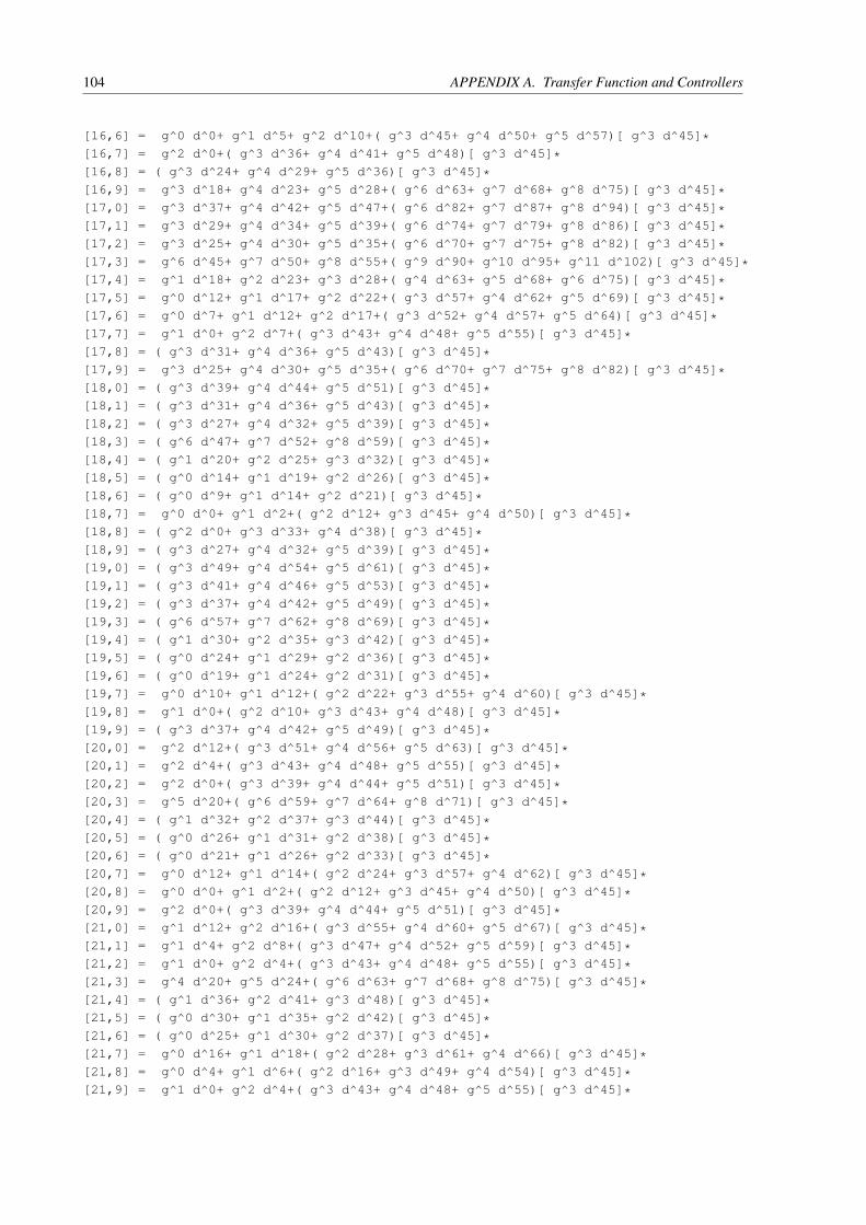
104 APPENDIX A. Transfer Function and Controllers
[16,6] = g^0 d^0+ g^1 d^5+ g^2 d^10+( g^3 d^45+ g^4 d^50+ g^5 d^57)[ g^3 d^45]*[16,7] = g^2 d^0+( g^3 d^36+ g^4 d^41+ g^5 d^48)[ g^3 d^45]*[16,8] = ( g^3 d^24+ g^4 d^29+ g^5 d^36)[ g^3 d^45]*[16,9] = g^3 d^18+ g^4 d^23+ g^5 d^28+( g^6 d^63+ g^7 d^68+ g^8 d^75)[ g^3 d^45]*[17,0] = g^3 d^37+ g^4 d^42+ g^5 d^47+( g^6 d^82+ g^7 d^87+ g^8 d^94)[ g^3 d^45]*[17,1] = g^3 d^29+ g^4 d^34+ g^5 d^39+( g^6 d^74+ g^7 d^79+ g^8 d^86)[ g^3 d^45]*[17,2] = g^3 d^25+ g^4 d^30+ g^5 d^35+( g^6 d^70+ g^7 d^75+ g^8 d^82)[ g^3 d^45]*[17,3] = g^6 d^45+ g^7 d^50+ g^8 d^55+( g^9 d^90+ g^10 d^95+ g^11 d^102)[ g^3 d^45]*[17,4] = g^1 d^18+ g^2 d^23+ g^3 d^28+( g^4 d^63+ g^5 d^68+ g^6 d^75)[ g^3 d^45]*[17,5] = g^0 d^12+ g^1 d^17+ g^2 d^22+( g^3 d^57+ g^4 d^62+ g^5 d^69)[ g^3 d^45]*[17,6] = g^0 d^7+ g^1 d^12+ g^2 d^17+( g^3 d^52+ g^4 d^57+ g^5 d^64)[ g^3 d^45]*[17,7] = g^1 d^0+ g^2 d^7+( g^3 d^43+ g^4 d^48+ g^5 d^55)[ g^3 d^45]*[17,8] = ( g^3 d^31+ g^4 d^36+ g^5 d^43)[ g^3 d^45]*[17,9] = g^3 d^25+ g^4 d^30+ g^5 d^35+( g^6 d^70+ g^7 d^75+ g^8 d^82)[ g^3 d^45]*[18,0] = ( g^3 d^39+ g^4 d^44+ g^5 d^51)[ g^3 d^45]*[18,1] = ( g^3 d^31+ g^4 d^36+ g^5 d^43)[ g^3 d^45]*[18,2] = ( g^3 d^27+ g^4 d^32+ g^5 d^39)[ g^3 d^45]*[18,3] = ( g^6 d^47+ g^7 d^52+ g^8 d^59)[ g^3 d^45]*[18,4] = ( g^1 d^20+ g^2 d^25+ g^3 d^32)[ g^3 d^45]*[18,5] = ( g^0 d^14+ g^1 d^19+ g^2 d^26)[ g^3 d^45]*[18,6] = ( g^0 d^9+ g^1 d^14+ g^2 d^21)[ g^3 d^45]*[18,7] = g^0 d^0+ g^1 d^2+( g^2 d^12+ g^3 d^45+ g^4 d^50)[ g^3 d^45]*[18,8] = ( g^2 d^0+ g^3 d^33+ g^4 d^38)[ g^3 d^45]*[18,9] = ( g^3 d^27+ g^4 d^32+ g^5 d^39)[ g^3 d^45]*[19,0] = ( g^3 d^49+ g^4 d^54+ g^5 d^61)[ g^3 d^45]*[19,1] = ( g^3 d^41+ g^4 d^46+ g^5 d^53)[ g^3 d^45]*[19,2] = ( g^3 d^37+ g^4 d^42+ g^5 d^49)[ g^3 d^45]*[19,3] = ( g^6 d^57+ g^7 d^62+ g^8 d^69)[ g^3 d^45]*[19,4] = ( g^1 d^30+ g^2 d^35+ g^3 d^42)[ g^3 d^45]*[19,5] = ( g^0 d^24+ g^1 d^29+ g^2 d^36)[ g^3 d^45]*[19,6] = ( g^0 d^19+ g^1 d^24+ g^2 d^31)[ g^3 d^45]*[19,7] = g^0 d^10+ g^1 d^12+( g^2 d^22+ g^3 d^55+ g^4 d^60)[ g^3 d^45]*[19,8] = g^1 d^0+( g^2 d^10+ g^3 d^43+ g^4 d^48)[ g^3 d^45]*[19,9] = ( g^3 d^37+ g^4 d^42+ g^5 d^49)[ g^3 d^45]*[20,0] = g^2 d^12+( g^3 d^51+ g^4 d^56+ g^5 d^63)[ g^3 d^45]*[20,1] = g^2 d^4+( g^3 d^43+ g^4 d^48+ g^5 d^55)[ g^3 d^45]*[20,2] = g^2 d^0+( g^3 d^39+ g^4 d^44+ g^5 d^51)[ g^3 d^45]*[20,3] = g^5 d^20+( g^6 d^59+ g^7 d^64+ g^8 d^71)[ g^3 d^45]*[20,4] = ( g^1 d^32+ g^2 d^37+ g^3 d^44)[ g^3 d^45]*[20,5] = ( g^0 d^26+ g^1 d^31+ g^2 d^38)[ g^3 d^45]*[20,6] = ( g^0 d^21+ g^1 d^26+ g^2 d^33)[ g^3 d^45]*[20,7] = g^0 d^12+ g^1 d^14+( g^2 d^24+ g^3 d^57+ g^4 d^62)[ g^3 d^45]*[20,8] = g^0 d^0+ g^1 d^2+( g^2 d^12+ g^3 d^45+ g^4 d^50)[ g^3 d^45]*[20,9] = g^2 d^0+( g^3 d^39+ g^4 d^44+ g^5 d^51)[ g^3 d^45]*[21,0] = g^1 d^12+ g^2 d^16+( g^3 d^55+ g^4 d^60+ g^5 d^67)[ g^3 d^45]*[21,1] = g^1 d^4+ g^2 d^8+( g^3 d^47+ g^4 d^52+ g^5 d^59)[ g^3 d^45]*[21,2] = g^1 d^0+ g^2 d^4+( g^3 d^43+ g^4 d^48+ g^5 d^55)[ g^3 d^45]*[21,3] = g^4 d^20+ g^5 d^24+( g^6 d^63+ g^7 d^68+ g^8 d^75)[ g^3 d^45]*[21,4] = ( g^1 d^36+ g^2 d^41+ g^3 d^48)[ g^3 d^45]*[21,5] = ( g^0 d^30+ g^1 d^35+ g^2 d^42)[ g^3 d^45]*[21,6] = ( g^0 d^25+ g^1 d^30+ g^2 d^37)[ g^3 d^45]*[21,7] = g^0 d^16+ g^1 d^18+( g^2 d^28+ g^3 d^61+ g^4 d^66)[ g^3 d^45]*[21,8] = g^0 d^4+ g^1 d^6+( g^2 d^16+ g^3 d^49+ g^4 d^54)[ g^3 d^45]*[21,9] = g^1 d^0+ g^2 d^4+( g^3 d^43+ g^4 d^48+ g^5 d^55)[ g^3 d^45]*
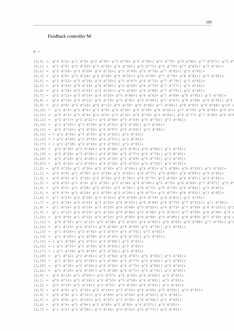
105
Feedback controller M:
M =
[0,0] = g^0 d^2+ g^1 d^4+ g^2 d^30+ g^3 d^34+ g^4 d^38+( g^5 d^75+ g^6 d^80+ g^7 d^87)[ g^3 d^45]*[0,1] = g^1 d^0+ g^2 d^26+ g^3 d^30+ g^4 d^34+( g^5 d^71+ g^6 d^76+ g^7 d^83)[ g^3 d^45]*[0,2] = g^2 d^24+ g^3 d^28+ g^4 d^32+( g^5 d^69+ g^6 d^74+ g^7 d^81)[ g^3 d^45]*[0,3] = g^2 d^0+ g^3 d^24+ g^4 d^28+ g^5 d^32+( g^6 d^69+ g^7 d^74+ g^8 d^81)[ g^3 d^45]*[0,4] = g^2 d^22+ g^3 d^26+ g^4 d^30+( g^5 d^67+ g^6 d^72+ g^7 d^79)[ g^3 d^45]*[0,5] = g^2 d^20+ g^3 d^24+ g^4 d^28+( g^5 d^65+ g^6 d^70+ g^7 d^77)[ g^3 d^45]*[0,6] = g^2 d^18+ g^3 d^22+ g^4 d^26+( g^5 d^63+ g^6 d^68+ g^7 d^75)[ g^3 d^45]*[0,7] = g^2 d^12+ g^3 d^16+ g^4 d^20+ g^5 d^46+( g^6 d^62+ g^7 d^69+ g^8 d^95)[ g^3 d^45]*[0,8] = g^2 d^10+ g^3 d^12+ g^4 d^18+ g^5 d^42+ g^6 d^46+( g^7 d^67+ g^8 d^88+ g^9 d^95)[ g^3 d^45]*[0,9] = g^2 d^8+ g^3 d^10+ g^4 d^12+ g^5 d^38+ g^6 d^42+ g^7 d^46+( g^8 d^83+ g^9 d^88+ g^10 d^95)[ g^3 d^45]*[0,10] = g^1 d^4+ g^2 d^6+ g^3 d^8+ g^4 d^34+ g^5 d^38+ g^6 d^42+( g^7 d^79+ g^8 d^84+ g^9 d^91)[ g^3 d^45]*[0,11] = g^0 d^2+ g^1 d^4+ g^2 d^6+ g^3 d^32+ g^4 d^36+ g^5 d^40+( g^6 d^77+ g^7 d^82+ g^8 d^89)[ g^3 d^45]*[0,12] = g^2 d^17+ g^3 d^21+( g^4 d^58+ g^5 d^63+ g^6 d^70)[ g^3 d^45]*[0,13] = g^2 d^18+( g^3 d^56+ g^4 d^61+ g^5 d^68)[ g^3 d^45]*[0,14] = g^2 d^14+( g^3 d^52+ g^4 d^57+ g^5 d^64)[ g^3 d^45]*[0,15] = ( g^2 d^50+ g^3 d^55+ g^4 d^62)[ g^3 d^45]*[0,16] = ( g^2 d^45+ g^3 d^50+ g^4 d^57)[ g^3 d^45]*[0,17] = ( g^2 d^38+ g^3 d^43+ g^4 d^50)[ g^3 d^45]*[0,18] = g^2 d^36+ g^3 d^40+( g^4 d^48+ g^5 d^81+ g^6 d^86)[ g^3 d^45]*[0,19] = g^2 d^26+ g^3 d^30+( g^4 d^38+ g^5 d^71+ g^6 d^76)[ g^3 d^45]*[0,20] = g^2 d^24+ g^3 d^28+( g^4 d^36+ g^5 d^69+ g^6 d^74)[ g^3 d^45]*[0,21] = g^2 d^20+ g^3 d^24+( g^4 d^32+ g^5 d^65+ g^6 d^70)[ g^3 d^45]*[1,0] = g^0 d^10+ g^1 d^36+ g^2 d^40+ g^3 d^44+( g^4 d^81+ g^5 d^86+ g^6 d^93)[ g^3 d^45]*[1,1] = g^0 d^6+ g^1 d^32+ g^2 d^36+ g^3 d^40+( g^4 d^77+ g^5 d^82+ g^6 d^89)[ g^3 d^45]*[1,2] = g^0 d^4+ g^1 d^30+ g^2 d^34+ g^3 d^38+( g^4 d^75+ g^5 d^80+ g^6 d^87)[ g^3 d^45]*[1,3] = g^0 d^2+ g^1 d^6+ g^2 d^30+ g^3 d^34+ g^4 d^38+( g^5 d^75+ g^6 d^80+ g^7 d^87)[ g^3 d^45]*[1,4] = g^0 d^2+ g^1 d^28+ g^2 d^32+ g^3 d^36+( g^4 d^73+ g^5 d^78+ g^6 d^85)[ g^3 d^45]*[1,5] = g^0 d^0+ g^1 d^26+ g^2 d^30+ g^3 d^34+( g^4 d^71+ g^5 d^76+ g^6 d^83)[ g^3 d^45]*[1,6] = g^1 d^24+ g^2 d^28+ g^3 d^32+( g^4 d^69+ g^5 d^74+ g^6 d^81)[ g^3 d^45]*[1,7] = g^1 d^18+ g^2 d^22+ g^3 d^26+ g^4 d^52+( g^5 d^68+ g^6 d^75+ g^7 d^101)[ g^3 d^45]*[1,8] = g^1 d^16+ g^2 d^18+ g^3 d^24+ g^4 d^48+ g^5 d^52+( g^6 d^73+ g^7 d^94+ g^8 d^101)[ g^3 d^45]*[1,9] = g^1 d^12+ g^2 d^16+ g^3 d^18+ g^4 d^44+ g^5 d^48+ g^6 d^52+( g^7 d^89+ g^8 d^94+ g^9 d^101)[ g^3 d^45]*[1,10] = g^0 d^8+ g^1 d^12+ g^2 d^14+ g^3 d^40+ g^4 d^44+ g^5 d^48+( g^6 d^85+ g^7 d^90+ g^8 d^97)[ g^3 d^45]*[1,11] = g^0 d^10+ g^1 d^12+ g^2 d^38+ g^3 d^42+ g^4 d^46+( g^5 d^83+ g^6 d^88+ g^7 d^95)[ g^3 d^45]*[1,12] = g^1 d^23+ g^2 d^27+( g^3 d^64+ g^4 d^69+ g^5 d^76)[ g^3 d^45]*[1,13] = g^1 d^24+( g^2 d^62+ g^3 d^67+ g^4 d^74)[ g^3 d^45]*[1,14] = g^1 d^20+( g^2 d^58+ g^3 d^63+ g^4 d^70)[ g^3 d^45]*[1,15] = ( g^1 d^56+ g^2 d^61+ g^3 d^68)[ g^3 d^45]*[1,16] = ( g^1 d^51+ g^2 d^56+ g^3 d^63)[ g^3 d^45]*[1,17] = ( g^1 d^44+ g^2 d^49+ g^3 d^56)[ g^3 d^45]*[1,18] = g^1 d^42+ g^2 d^46+( g^3 d^54+ g^4 d^87+ g^5 d^92)[ g^3 d^45]*[1,19] = g^1 d^32+ g^2 d^36+( g^3 d^44+ g^4 d^77+ g^5 d^82)[ g^3 d^45]*[1,20] = g^1 d^30+ g^2 d^34+( g^3 d^42+ g^4 d^75+ g^5 d^80)[ g^3 d^45]*[1,21] = g^1 d^26+ g^2 d^30+( g^3 d^38+ g^4 d^71+ g^5 d^76)[ g^3 d^45]*[2,0] = g^0 d^16+ g^1 d^20+( g^2 d^57+ g^3 d^62+ g^4 d^69)[ g^3 d^45]*[2,1] = g^0 d^12+ g^1 d^16+( g^2 d^53+ g^3 d^58+ g^4 d^65)[ g^3 d^45]*[2,2] = g^0 d^10+ g^1 d^14+( g^2 d^51+ g^3 d^56+ g^4 d^63)[ g^3 d^45]*[2,3] = g^0 d^6+ g^1 d^10+ g^2 d^14+( g^3 d^51+ g^4 d^56+ g^5 d^63)[ g^3 d^45]*[2,4] = g^0 d^8+ g^1 d^12+( g^2 d^49+ g^3 d^54+ g^4 d^61)[ g^3 d^45]*[2,5] = g^0 d^6+ g^1 d^10+( g^2 d^47+ g^3 d^52+ g^4 d^59)[ g^3 d^45]*[2,6] = g^0 d^4+ g^1 d^8+( g^2 d^45+ g^3 d^50+ g^4 d^57)[ g^3 d^45]*[2,7] = g^1 d^2+ g^2 d^28+( g^3 d^44+ g^4 d^51+ g^5 d^77)[ g^3 d^45]*

106 APPENDIX A. Transfer Function and Controllers
[2,8] = g^1 d^0+ g^2 d^24+ g^3 d^28+( g^4 d^49+ g^5 d^70+ g^6 d^77)[ g^3 d^45]*[2,9] = g^2 d^20+ g^3 d^24+ g^4 d^28+( g^5 d^65+ g^6 d^70+ g^7 d^77)[ g^3 d^45]*[2,10] = g^1 d^16+ g^2 d^20+ g^3 d^24+( g^4 d^61+ g^5 d^66+ g^6 d^73)[ g^3 d^45]*[2,11] = g^0 d^14+ g^1 d^18+ g^2 d^22+( g^3 d^59+ g^4 d^64+ g^5 d^71)[ g^3 d^45]*[2,12] = g^0 d^3+( g^1 d^40+ g^2 d^45+ g^3 d^52)[ g^3 d^45]*[2,13] = ( g^0 d^38+ g^1 d^43+ g^2 d^50)[ g^3 d^45]*[2,14] = ( g^0 d^34+ g^1 d^39+ g^2 d^46)[ g^3 d^45]*[2,15] = ( g^0 d^37+ g^1 d^44+ g^2 d^77)[ g^3 d^45]*[2,16] = ( g^0 d^32+ g^1 d^39+ g^2 d^72)[ g^3 d^45]*[2,17] = ( g^0 d^25+ g^1 d^32+ g^2 d^65)[ g^3 d^45]*[2,18] = g^0 d^22+( g^1 d^30+ g^2 d^63+ g^3 d^68)[ g^3 d^45]*[2,19] = g^0 d^12+( g^1 d^20+ g^2 d^53+ g^3 d^58)[ g^3 d^45]*[2,20] = g^0 d^10+( g^1 d^18+ g^2 d^51+ g^3 d^56)[ g^3 d^45]*[2,21] = g^0 d^6+( g^1 d^14+ g^2 d^47+ g^3 d^52)[ g^3 d^45]*[3,0] = g^0 d^26+ g^1 d^30+( g^2 d^67+ g^3 d^72+ g^4 d^79)[ g^3 d^45]*[3,1] = g^0 d^22+ g^1 d^26+( g^2 d^63+ g^3 d^68+ g^4 d^75)[ g^3 d^45]*[3,2] = g^0 d^20+ g^1 d^24+( g^2 d^61+ g^3 d^66+ g^4 d^73)[ g^3 d^45]*[3,3] = g^0 d^16+ g^1 d^20+ g^2 d^24+( g^3 d^61+ g^4 d^66+ g^5 d^73)[ g^3 d^45]*[3,4] = g^0 d^18+ g^1 d^22+( g^2 d^59+ g^3 d^64+ g^4 d^71)[ g^3 d^45]*[3,5] = g^0 d^16+ g^1 d^20+( g^2 d^57+ g^3 d^62+ g^4 d^69)[ g^3 d^45]*[3,6] = g^0 d^14+ g^1 d^18+( g^2 d^55+ g^3 d^60+ g^4 d^67)[ g^3 d^45]*[3,7] = g^0 d^8+ g^1 d^12+ g^2 d^38+( g^3 d^54+ g^4 d^61+ g^5 d^87)[ g^3 d^45]*[3,8] = g^0 d^4+ g^1 d^10+ g^2 d^34+ g^3 d^38+( g^4 d^59+ g^5 d^80+ g^6 d^87)[ g^3 d^45]*[3,9] = g^0 d^2+ g^1 d^4+ g^2 d^30+ g^3 d^34+ g^4 d^38+( g^5 d^75+ g^6 d^80+ g^7 d^87)[ g^3 d^45]*[3,10] = g^0 d^0+ g^1 d^26+ g^2 d^30+ g^3 d^34+( g^4 d^71+ g^5 d^76+ g^6 d^83)[ g^3 d^45]*[3,11] = g^0 d^24+ g^1 d^28+ g^2 d^32+( g^3 d^69+ g^4 d^74+ g^5 d^81)[ g^3 d^45]*[3,12] = g^0 d^13+( g^1 d^50+ g^2 d^55+ g^3 d^62)[ g^3 d^45]*[3,13] = ( g^0 d^48+ g^1 d^53+ g^2 d^60)[ g^3 d^45]*[3,14] = ( g^0 d^44+ g^1 d^49+ g^2 d^56)[ g^3 d^45]*[3,15] = ( g^0 d^47+ g^1 d^54+ g^2 d^87)[ g^3 d^45]*[3,16] = ( g^0 d^42+ g^1 d^49+ g^2 d^82)[ g^3 d^45]*[3,17] = ( g^0 d^35+ g^1 d^42+ g^2 d^75)[ g^3 d^45]*[3,18] = g^0 d^32+( g^1 d^40+ g^2 d^73+ g^3 d^78)[ g^3 d^45]*[3,19] = g^0 d^22+( g^1 d^30+ g^2 d^63+ g^3 d^68)[ g^3 d^45]*[3,20] = g^0 d^20+( g^1 d^28+ g^2 d^61+ g^3 d^66)[ g^3 d^45]*[3,21] = g^0 d^16+( g^1 d^24+ g^2 d^57+ g^3 d^62)[ g^3 d^45]*[4,0] = g^1 d^19+ g^2 d^23+ g^3 d^27+( g^4 d^64+ g^5 d^69+ g^6 d^76)[ g^3 d^45]*[4,1] = g^1 d^15+ g^2 d^19+ g^3 d^23+( g^4 d^60+ g^5 d^65+ g^6 d^72)[ g^3 d^45]*[4,2] = g^1 d^13+ g^2 d^17+ g^3 d^21+( g^4 d^58+ g^5 d^63+ g^6 d^70)[ g^3 d^45]*[4,3] = g^2 d^13+ g^3 d^17+ g^4 d^21+( g^5 d^58+ g^6 d^63+ g^7 d^70)[ g^3 d^45]*[4,4] = g^1 d^11+ g^2 d^15+ g^3 d^19+( g^4 d^56+ g^5 d^61+ g^6 d^68)[ g^3 d^45]*[4,5] = g^1 d^9+ g^2 d^13+ g^3 d^17+( g^4 d^54+ g^5 d^59+ g^6 d^66)[ g^3 d^45]*[4,6] = g^1 d^7+ g^2 d^11+ g^3 d^15+( g^4 d^52+ g^5 d^57+ g^6 d^64)[ g^3 d^45]*[4,7] = g^2 d^5+ g^3 d^9+ g^4 d^35+( g^5 d^51+ g^6 d^58+ g^7 d^84)[ g^3 d^45]*[4,8] = g^3 d^7+ g^4 d^31+ g^5 d^35+( g^6 d^56+ g^7 d^77+ g^8 d^84)[ g^3 d^45]*[4,9] = g^4 d^27+ g^5 d^31+ g^6 d^35+( g^7 d^72+ g^8 d^77+ g^9 d^84)[ g^3 d^45]*[4,10] = g^3 d^23+ g^4 d^27+ g^5 d^31+( g^6 d^68+ g^7 d^73+ g^8 d^80)[ g^3 d^45]*[4,11] = g^2 d^21+ g^3 d^25+ g^4 d^29+( g^5 d^66+ g^6 d^71+ g^7 d^78)[ g^3 d^45]*[4,12] = g^0 d^2+ g^1 d^6+ g^2 d^10+( g^3 d^47+ g^4 d^52+ g^5 d^59)[ g^3 d^45]*[4,13] = g^0 d^2+ g^1 d^7+( g^2 d^45+ g^3 d^50+ g^4 d^57)[ g^3 d^45]*[4,14] = g^1 d^3+( g^2 d^41+ g^3 d^46+ g^4 d^53)[ g^3 d^45]*[4,15] = g^0 d^1+( g^1 d^39+ g^2 d^44+ g^3 d^51)[ g^3 d^45]*[4,16] = ( g^1 d^34+ g^2 d^39+ g^3 d^46)[ g^3 d^45]*[4,17] = ( g^1 d^27+ g^2 d^32+ g^3 d^39)[ g^3 d^45]*[4,18] = g^1 d^25+ g^2 d^29+( g^3 d^37+ g^4 d^70+ g^5 d^75)[ g^3 d^45]*[4,19] = g^1 d^15+ g^2 d^19+( g^3 d^27+ g^4 d^60+ g^5 d^65)[ g^3 d^45]*[4,20] = g^1 d^13+ g^2 d^17+( g^3 d^25+ g^4 d^58+ g^5 d^63)[ g^3 d^45]*

107
[4,21] = g^1 d^9+ g^2 d^13+( g^3 d^21+ g^4 d^54+ g^5 d^59)[ g^3 d^45]*[5,0] = g^2 d^25+ g^3 d^30+ g^4 d^35+( g^5 d^70+ g^6 d^75+ g^7 d^82)[ g^3 d^45]*[5,1] = g^2 d^21+ g^3 d^26+ g^4 d^31+( g^5 d^66+ g^6 d^71+ g^7 d^78)[ g^3 d^45]*[5,2] = g^2 d^19+ g^3 d^24+ g^4 d^29+( g^5 d^64+ g^6 d^69+ g^7 d^76)[ g^3 d^45]*[5,3] = g^3 d^19+ g^4 d^24+ g^5 d^29+( g^6 d^64+ g^7 d^69+ g^8 d^76)[ g^3 d^45]*[5,4] = g^2 d^17+ g^3 d^22+ g^4 d^27+( g^5 d^62+ g^6 d^67+ g^7 d^74)[ g^3 d^45]*[5,5] = g^2 d^15+ g^3 d^20+ g^4 d^25+( g^5 d^60+ g^6 d^65+ g^7 d^72)[ g^3 d^45]*[5,6] = g^2 d^13+ g^3 d^18+ g^4 d^23+( g^5 d^58+ g^6 d^63+ g^7 d^70)[ g^3 d^45]*[5,7] = g^3 d^12+ g^4 d^17+ g^5 d^43+( g^6 d^57+ g^7 d^64+ g^8 d^90)[ g^3 d^45]*[5,8] = g^4 d^15+ g^5 d^38+ g^6 d^43+( g^7 d^62+ g^8 d^83+ g^9 d^90)[ g^3 d^45]*[5,9] = g^5 d^33+ g^6 d^38+ g^7 d^43+( g^8 d^78+ g^9 d^83+ g^10 d^90)[ g^3 d^45]*[5,10] = g^4 d^29+ g^5 d^34+ g^6 d^39+( g^7 d^74+ g^8 d^79+ g^9 d^86)[ g^3 d^45]*[5,11] = g^3 d^27+ g^4 d^32+ g^5 d^37+( g^6 d^72+ g^7 d^77+ g^8 d^84)[ g^3 d^45]*[5,12] = g^1 d^8+ g^2 d^13+ g^3 d^18+( g^4 d^53+ g^5 d^58+ g^6 d^65)[ g^3 d^45]*[5,13] = g^0 d^6+ g^1 d^11+ g^2 d^16+( g^3 d^51+ g^4 d^56+ g^5 d^63)[ g^3 d^45]*[5,14] = g^0 d^2+ g^1 d^7+ g^2 d^12+( g^3 d^47+ g^4 d^52+ g^5 d^59)[ g^3 d^45]*[5,15] = g^0 d^5+ g^1 d^10+( g^2 d^45+ g^3 d^50+ g^4 d^57)[ g^3 d^45]*[5,16] = g^0 d^0+ g^1 d^5+( g^2 d^40+ g^3 d^45+ g^4 d^52)[ g^3 d^45]*[5,17] = ( g^2 d^33+ g^3 d^38+ g^4 d^45)[ g^3 d^45]*[5,18] = ( g^2 d^31+ g^3 d^36+ g^4 d^43)[ g^3 d^45]*[5,19] = ( g^2 d^21+ g^3 d^26+ g^4 d^33)[ g^3 d^45]*[5,20] = ( g^2 d^19+ g^3 d^24+ g^4 d^31)[ g^3 d^45]*[5,21] = ( g^2 d^15+ g^3 d^20+ g^4 d^27)[ g^3 d^45]*[6,0] = g^2 d^30+ g^3 d^35+ g^4 d^40+( g^5 d^75+ g^6 d^80+ g^7 d^87)[ g^3 d^45]*[6,1] = g^2 d^26+ g^3 d^31+ g^4 d^36+( g^5 d^71+ g^6 d^76+ g^7 d^83)[ g^3 d^45]*[6,2] = g^2 d^24+ g^3 d^29+ g^4 d^34+( g^5 d^69+ g^6 d^74+ g^7 d^81)[ g^3 d^45]*[6,3] = g^3 d^24+ g^4 d^29+ g^5 d^34+( g^6 d^69+ g^7 d^74+ g^8 d^81)[ g^3 d^45]*[6,4] = g^2 d^22+ g^3 d^27+ g^4 d^32+( g^5 d^67+ g^6 d^72+ g^7 d^79)[ g^3 d^45]*[6,5] = g^2 d^20+ g^3 d^25+ g^4 d^30+( g^5 d^65+ g^6 d^70+ g^7 d^77)[ g^3 d^45]*[6,6] = g^2 d^18+ g^3 d^23+ g^4 d^28+( g^5 d^63+ g^6 d^68+ g^7 d^75)[ g^3 d^45]*[6,7] = g^3 d^17+ g^4 d^22+ g^5 d^48+( g^6 d^62+ g^7 d^69+ g^8 d^95)[ g^3 d^45]*[6,8] = g^4 d^20+ g^5 d^43+ g^6 d^48+( g^7 d^67+ g^8 d^88+ g^9 d^95)[ g^3 d^45]*[6,9] = g^5 d^38+ g^6 d^43+ g^7 d^48+( g^8 d^83+ g^9 d^88+ g^10 d^95)[ g^3 d^45]*[6,10] = g^4 d^34+ g^5 d^39+ g^6 d^44+( g^7 d^79+ g^8 d^84+ g^9 d^91)[ g^3 d^45]*[6,11] = g^3 d^32+ g^4 d^37+ g^5 d^42+( g^6 d^77+ g^7 d^82+ g^8 d^89)[ g^3 d^45]*[6,12] = g^1 d^13+ g^2 d^18+ g^3 d^23+( g^4 d^58+ g^5 d^63+ g^6 d^70)[ g^3 d^45]*[6,13] = g^0 d^11+ g^1 d^16+ g^2 d^21+( g^3 d^56+ g^4 d^61+ g^5 d^68)[ g^3 d^45]*[6,14] = g^0 d^7+ g^1 d^12+ g^2 d^17+( g^3 d^52+ g^4 d^57+ g^5 d^64)[ g^3 d^45]*[6,15] = g^0 d^10+ g^1 d^15+( g^2 d^50+ g^3 d^55+ g^4 d^62)[ g^3 d^45]*[6,16] = g^0 d^5+ g^1 d^10+( g^2 d^45+ g^3 d^50+ g^4 d^57)[ g^3 d^45]*[6,17] = g^1 d^3+( g^2 d^38+ g^3 d^43+ g^4 d^50)[ g^3 d^45]*[6,18] = g^1 d^0+( g^2 d^36+ g^3 d^41+ g^4 d^48)[ g^3 d^45]*[6,19] = ( g^2 d^26+ g^3 d^31+ g^4 d^38)[ g^3 d^45]*[6,20] = ( g^2 d^24+ g^3 d^29+ g^4 d^36)[ g^3 d^45]*[6,21] = ( g^2 d^20+ g^3 d^25+ g^4 d^32)[ g^3 d^45]*[7,0] = ( g^2 d^39+ g^3 d^44+ g^4 d^51)[ g^3 d^45]*[7,1] = ( g^2 d^35+ g^3 d^40+ g^4 d^47)[ g^3 d^45]*[7,2] = ( g^2 d^33+ g^3 d^38+ g^4 d^45)[ g^3 d^45]*[7,3] = ( g^3 d^33+ g^4 d^38+ g^5 d^45)[ g^3 d^45]*[7,4] = ( g^2 d^31+ g^3 d^36+ g^4 d^43)[ g^3 d^45]*[7,5] = ( g^2 d^29+ g^3 d^34+ g^4 d^41)[ g^3 d^45]*[7,6] = ( g^2 d^27+ g^3 d^32+ g^4 d^39)[ g^3 d^45]*[7,7] = ( g^3 d^26+ g^4 d^33+ g^5 d^59)[ g^3 d^45]*[7,8] = ( g^4 d^31+ g^5 d^52+ g^6 d^59)[ g^3 d^45]*[7,9] = ( g^5 d^47+ g^6 d^52+ g^7 d^59)[ g^3 d^45]*[7,10] = ( g^4 d^43+ g^5 d^48+ g^6 d^55)[ g^3 d^45]*[7,11] = ( g^3 d^41+ g^4 d^46+ g^5 d^53)[ g^3 d^45]*
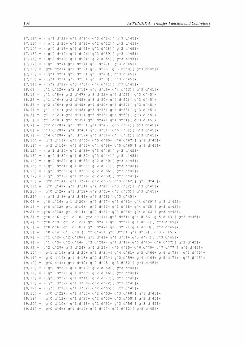
108 APPENDIX A. Transfer Function and Controllers
[7,12] = ( g^1 d^22+ g^2 d^27+ g^3 d^34)[ g^3 d^45]*[7,13] = ( g^0 d^20+ g^1 d^25+ g^2 d^32)[ g^3 d^45]*[7,14] = ( g^0 d^16+ g^1 d^21+ g^2 d^28)[ g^3 d^45]*[7,15] = ( g^0 d^19+ g^1 d^26+ g^2 d^59)[ g^3 d^45]*[7,16] = ( g^0 d^14+ g^1 d^21+ g^2 d^54)[ g^3 d^45]*[7,17] = ( g^0 d^7+ g^1 d^14+ g^2 d^47)[ g^3 d^45]*[7,18] = g^0 d^2+( g^1 d^12+ g^2 d^45+ g^3 d^50)[ g^3 d^45]*[7,19] = ( g^1 d^2+ g^2 d^35+ g^3 d^40)[ g^3 d^45]*[7,20] = ( g^1 d^0+ g^2 d^33+ g^3 d^38)[ g^3 d^45]*[7,21] = ( g^2 d^29+ g^3 d^34+ g^4 d^41)[ g^3 d^45]*[8,0] = g^1 d^12+( g^2 d^51+ g^3 d^56+ g^4 d^63)[ g^3 d^45]*[8,1] = g^1 d^8+( g^2 d^47+ g^3 d^52+ g^4 d^59)[ g^3 d^45]*[8,2] = g^1 d^6+( g^2 d^45+ g^3 d^50+ g^4 d^57)[ g^3 d^45]*[8,3] = g^2 d^6+( g^3 d^45+ g^4 d^50+ g^5 d^57)[ g^3 d^45]*[8,4] = g^1 d^4+( g^2 d^43+ g^3 d^48+ g^4 d^55)[ g^3 d^45]*[8,5] = g^1 d^2+( g^2 d^41+ g^3 d^46+ g^4 d^53)[ g^3 d^45]*[8,6] = g^1 d^0+( g^2 d^39+ g^3 d^44+ g^4 d^51)[ g^3 d^45]*[8,7] = g^2 d^20+( g^3 d^38+ g^4 d^45+ g^5 d^71)[ g^3 d^45]*[8,8] = g^3 d^20+( g^4 d^43+ g^5 d^64+ g^6 d^71)[ g^3 d^45]*[8,9] = g^4 d^20+( g^5 d^59+ g^6 d^64+ g^7 d^71)[ g^3 d^45]*[8,10] = g^3 d^16+( g^4 d^55+ g^5 d^60+ g^6 d^67)[ g^3 d^45]*[8,11] = g^2 d^14+( g^3 d^53+ g^4 d^58+ g^5 d^65)[ g^3 d^45]*[8,12] = ( g^1 d^34+ g^2 d^39+ g^3 d^46)[ g^3 d^45]*[8,13] = ( g^0 d^32+ g^1 d^37+ g^2 d^44)[ g^3 d^45]*[8,14] = ( g^0 d^28+ g^1 d^33+ g^2 d^40)[ g^3 d^45]*[8,15] = ( g^0 d^31+ g^1 d^38+ g^2 d^71)[ g^3 d^45]*[8,16] = ( g^0 d^26+ g^1 d^33+ g^2 d^66)[ g^3 d^45]*[8,17] = ( g^0 d^19+ g^1 d^26+ g^2 d^59)[ g^3 d^45]*[8,18] = g^0 d^14+( g^1 d^24+ g^2 d^57+ g^3 d^62)[ g^3 d^45]*[8,19] = g^0 d^4+( g^1 d^14+ g^2 d^47+ g^3 d^52)[ g^3 d^45]*[8,20] = g^0 d^2+( g^1 d^12+ g^2 d^45+ g^3 d^50)[ g^3 d^45]*[8,21] = ( g^1 d^8+ g^2 d^41+ g^3 d^46)[ g^3 d^45]*[9,0] = g^0 d^16+ g^1 d^20+( g^2 d^57+ g^3 d^62+ g^4 d^69)[ g^3 d^45]*[9,1] = g^0 d^12+ g^1 d^16+( g^2 d^53+ g^3 d^58+ g^4 d^65)[ g^3 d^45]*[9,2] = g^0 d^10+ g^1 d^14+( g^2 d^51+ g^3 d^56+ g^4 d^63)[ g^3 d^45]*[9,3] = g^0 d^6+ g^1 d^10+ g^2 d^14+( g^3 d^51+ g^4 d^56+ g^5 d^63)[ g^3 d^45]*[9,4] = g^0 d^8+ g^1 d^12+( g^2 d^49+ g^3 d^54+ g^4 d^61)[ g^3 d^45]*[9,5] = g^0 d^6+ g^1 d^10+( g^2 d^47+ g^3 d^52+ g^4 d^59)[ g^3 d^45]*[9,6] = g^0 d^4+ g^1 d^8+( g^2 d^45+ g^3 d^50+ g^4 d^57)[ g^3 d^45]*[9,7] = g^1 d^2+ g^2 d^28+( g^3 d^44+ g^4 d^51+ g^5 d^77)[ g^3 d^45]*[9,8] = g^1 d^0+ g^2 d^24+ g^3 d^28+( g^4 d^49+ g^5 d^70+ g^6 d^77)[ g^3 d^45]*[9,9] = g^2 d^20+ g^3 d^24+ g^4 d^28+( g^5 d^65+ g^6 d^70+ g^7 d^77)[ g^3 d^45]*[9,10] = g^1 d^16+ g^2 d^20+ g^3 d^24+( g^4 d^61+ g^5 d^66+ g^6 d^73)[ g^3 d^45]*[9,11] = g^0 d^14+ g^1 d^18+ g^2 d^22+( g^3 d^59+ g^4 d^64+ g^5 d^71)[ g^3 d^45]*[9,12] = g^0 d^3+( g^1 d^40+ g^2 d^45+ g^3 d^52)[ g^3 d^45]*[9,13] = ( g^0 d^38+ g^1 d^43+ g^2 d^50)[ g^3 d^45]*[9,14] = ( g^0 d^34+ g^1 d^39+ g^2 d^46)[ g^3 d^45]*[9,15] = ( g^0 d^37+ g^1 d^44+ g^2 d^77)[ g^3 d^45]*[9,16] = ( g^0 d^32+ g^1 d^39+ g^2 d^72)[ g^3 d^45]*[9,17] = ( g^0 d^25+ g^1 d^32+ g^2 d^65)[ g^3 d^45]*[9,18] = g^0 d^22+( g^1 d^30+ g^2 d^63+ g^3 d^68)[ g^3 d^45]*[9,19] = g^0 d^12+( g^1 d^20+ g^2 d^53+ g^3 d^58)[ g^3 d^45]*[9,20] = g^0 d^10+( g^1 d^18+ g^2 d^51+ g^3 d^56)[ g^3 d^45]*[9,21] = g^0 d^6+( g^1 d^14+ g^2 d^47+ g^3 d^52)[ g^3 d^45]*

109
The matrix K is given by:
K =
[0,0] = g^0 d^2+ g^1 d^4+ g^2 d^30+ g^3 d^34+ g^4 d^38+( g^5 d^75+ g^6 d^80+ g^7 d^87)[ g^3 d^45]*[0,1] = g^2 d^22+ g^3 d^26+ g^4 d^30+( g^5 d^67+ g^6 d^72+ g^7 d^79)[ g^3 d^45]*[0,2] = g^2 d^18+ g^3 d^22+ g^4 d^26+( g^5 d^63+ g^6 d^68+ g^7 d^75)[ g^3 d^45]*[0,3] = g^2 d^8+ g^3 d^10+ g^4 d^12+ g^5 d^38+ g^6 d^42+ g^7 d^46+( g^8 d^83+ g^9 d^88+ g^10 d^95)[ g^3 d^45]*[0,4] = g^2 d^18+( g^3 d^56+ g^4 d^61+ g^5 d^68)[ g^3 d^45]*[0,5] = ( g^2 d^50+ g^3 d^55+ g^4 d^62)[ g^3 d^45]*[0,6] = ( g^2 d^45+ g^3 d^50+ g^4 d^57)[ g^3 d^45]*[0,7] = g^2 d^36+ g^3 d^40+( g^4 d^48+ g^5 d^81+ g^6 d^86)[ g^3 d^45]*[0,8] = g^2 d^24+ g^3 d^28+( g^4 d^36+ g^5 d^69+ g^6 d^74)[ g^3 d^45]*[0,9] = g^2 d^18+ g^3 d^22+ g^4 d^26+( g^5 d^63+ g^6 d^68+ g^7 d^75)[ g^3 d^45]*[1,0] = g^0 d^10+ g^1 d^36+ g^2 d^40+ g^3 d^44+( g^4 d^81+ g^5 d^86+ g^6 d^93)[ g^3 d^45]*[1,1] = g^0 d^2+ g^1 d^28+ g^2 d^32+ g^3 d^36+( g^4 d^73+ g^5 d^78+ g^6 d^85)[ g^3 d^45]*[1,2] = g^1 d^24+ g^2 d^28+ g^3 d^32+( g^4 d^69+ g^5 d^74+ g^6 d^81)[ g^3 d^45]*[1,3] = g^1 d^12+ g^2 d^16+ g^3 d^18+ g^4 d^44+ g^5 d^48+ g^6 d^52+( g^7 d^89+ g^8 d^94+ g^9 d^101)[ g^3 d^45]*[1,4] = g^1 d^24+( g^2 d^62+ g^3 d^67+ g^4 d^74)[ g^3 d^45]*[1,5] = ( g^1 d^56+ g^2 d^61+ g^3 d^68)[ g^3 d^45]*[1,6] = ( g^1 d^51+ g^2 d^56+ g^3 d^63)[ g^3 d^45]*[1,7] = g^1 d^42+ g^2 d^46+( g^3 d^54+ g^4 d^87+ g^5 d^92)[ g^3 d^45]*[1,8] = g^1 d^30+ g^2 d^34+( g^3 d^42+ g^4 d^75+ g^5 d^80)[ g^3 d^45]*[1,9] = g^1 d^24+ g^2 d^28+ g^3 d^32+( g^4 d^69+ g^5 d^74+ g^6 d^81)[ g^3 d^45]*[2,0] = g^0 d^16+ g^1 d^20+( g^2 d^57+ g^3 d^62+ g^4 d^69)[ g^3 d^45]*[2,1] = g^0 d^8+ g^1 d^12+( g^2 d^49+ g^3 d^54+ g^4 d^61)[ g^3 d^45]*[2,2] = g^0 d^4+ g^1 d^8+( g^2 d^45+ g^3 d^50+ g^4 d^57)[ g^3 d^45]*[2,3] = g^2 d^20+ g^3 d^24+ g^4 d^28+( g^5 d^65+ g^6 d^70+ g^7 d^77)[ g^3 d^45]*[2,4] = ( g^0 d^38+ g^1 d^43+ g^2 d^50)[ g^3 d^45]*[2,5] = ( g^0 d^37+ g^1 d^44+ g^2 d^77)[ g^3 d^45]*[2,6] = ( g^0 d^32+ g^1 d^39+ g^2 d^72)[ g^3 d^45]*[2,7] = g^0 d^22+( g^1 d^30+ g^2 d^63+ g^3 d^68)[ g^3 d^45]*[2,8] = g^0 d^10+( g^1 d^18+ g^2 d^51+ g^3 d^56)[ g^3 d^45]*[2,9] = g^0 d^4+ g^1 d^8+( g^2 d^45+ g^3 d^50+ g^4 d^57)[ g^3 d^45]*[3,0] = g^0 d^26+ g^1 d^30+( g^2 d^67+ g^3 d^72+ g^4 d^79)[ g^3 d^45]*[3,1] = g^0 d^18+ g^1 d^22+( g^2 d^59+ g^3 d^64+ g^4 d^71)[ g^3 d^45]*[3,2] = g^0 d^14+ g^1 d^18+( g^2 d^55+ g^3 d^60+ g^4 d^67)[ g^3 d^45]*[3,3] = g^0 d^2+ g^1 d^4+ g^2 d^30+ g^3 d^34+ g^4 d^38+( g^5 d^75+ g^6 d^80+ g^7 d^87)[ g^3 d^45]*[3,4] = ( g^0 d^48+ g^1 d^53+ g^2 d^60)[ g^3 d^45]*[3,5] = ( g^0 d^47+ g^1 d^54+ g^2 d^87)[ g^3 d^45]*[3,6] = ( g^0 d^42+ g^1 d^49+ g^2 d^82)[ g^3 d^45]*[3,7] = g^0 d^32+( g^1 d^40+ g^2 d^73+ g^3 d^78)[ g^3 d^45]*[3,8] = g^0 d^20+( g^1 d^28+ g^2 d^61+ g^3 d^66)[ g^3 d^45]*[3,9] = g^0 d^14+ g^1 d^18+( g^2 d^55+ g^3 d^60+ g^4 d^67)[ g^3 d^45]*[4,0] = g^1 d^19+ g^2 d^23+ g^3 d^27+( g^4 d^64+ g^5 d^69+ g^6 d^76)[ g^3 d^45]*[4,1] = g^1 d^11+ g^2 d^15+ g^3 d^19+( g^4 d^56+ g^5 d^61+ g^6 d^68)[ g^3 d^45]*[4,2] = g^1 d^7+ g^2 d^11+ g^3 d^15+( g^4 d^52+ g^5 d^57+ g^6 d^64)[ g^3 d^45]*[4,3] = g^4 d^27+ g^5 d^31+ g^6 d^35+( g^7 d^72+ g^8 d^77+ g^9 d^84)[ g^3 d^45]*[4,4] = g^0 d^2+ g^1 d^7+( g^2 d^45+ g^3 d^50+ g^4 d^57)[ g^3 d^45]*[4,5] = g^0 d^1+( g^1 d^39+ g^2 d^44+ g^3 d^51)[ g^3 d^45]*[4,6] = ( g^1 d^34+ g^2 d^39+ g^3 d^46)[ g^3 d^45]*[4,7] = g^1 d^25+ g^2 d^29+( g^3 d^37+ g^4 d^70+ g^5 d^75)[ g^3 d^45]*[4,8] = g^1 d^13+ g^2 d^17+( g^3 d^25+ g^4 d^58+ g^5 d^63)[ g^3 d^45]*[4,9] = g^1 d^7+ g^2 d^11+ g^3 d^15+( g^4 d^52+ g^5 d^57+ g^6 d^64)[ g^3 d^45]*[5,0] = g^2 d^25+ g^3 d^30+ g^4 d^35+( g^5 d^70+ g^6 d^75+ g^7 d^82)[ g^3 d^45]*[5,1] = g^2 d^17+ g^3 d^22+ g^4 d^27+( g^5 d^62+ g^6 d^67+ g^7 d^74)[ g^3 d^45]*

110 APPENDIX A. Transfer Function and Controllers
[5,2] = g^2 d^13+ g^3 d^18+ g^4 d^23+( g^5 d^58+ g^6 d^63+ g^7 d^70)[ g^3 d^45]*[5,3] = g^5 d^33+ g^6 d^38+ g^7 d^43+( g^8 d^78+ g^9 d^83+ g^10 d^90)[ g^3 d^45]*[5,4] = g^0 d^6+ g^1 d^11+ g^2 d^16+( g^3 d^51+ g^4 d^56+ g^5 d^63)[ g^3 d^45]*[5,5] = g^0 d^5+ g^1 d^10+( g^2 d^45+ g^3 d^50+ g^4 d^57)[ g^3 d^45]*[5,6] = g^0 d^0+ g^1 d^5+( g^2 d^40+ g^3 d^45+ g^4 d^52)[ g^3 d^45]*[5,7] = ( g^2 d^31+ g^3 d^36+ g^4 d^43)[ g^3 d^45]*[5,8] = ( g^2 d^19+ g^3 d^24+ g^4 d^31)[ g^3 d^45]*[5,9] = g^2 d^13+ g^3 d^18+ g^4 d^23+( g^5 d^58+ g^6 d^63+ g^7 d^70)[ g^3 d^45]*[6,0] = g^2 d^30+ g^3 d^35+ g^4 d^40+( g^5 d^75+ g^6 d^80+ g^7 d^87)[ g^3 d^45]*[6,1] = g^2 d^22+ g^3 d^27+ g^4 d^32+( g^5 d^67+ g^6 d^72+ g^7 d^79)[ g^3 d^45]*[6,2] = g^2 d^18+ g^3 d^23+ g^4 d^28+( g^5 d^63+ g^6 d^68+ g^7 d^75)[ g^3 d^45]*[6,3] = g^5 d^38+ g^6 d^43+ g^7 d^48+( g^8 d^83+ g^9 d^88+ g^10 d^95)[ g^3 d^45]*[6,4] = g^0 d^11+ g^1 d^16+ g^2 d^21+( g^3 d^56+ g^4 d^61+ g^5 d^68)[ g^3 d^45]*[6,5] = g^0 d^10+ g^1 d^15+( g^2 d^50+ g^3 d^55+ g^4 d^62)[ g^3 d^45]*[6,6] = g^0 d^5+ g^1 d^10+( g^2 d^45+ g^3 d^50+ g^4 d^57)[ g^3 d^45]*[6,7] = g^1 d^0+( g^2 d^36+ g^3 d^41+ g^4 d^48)[ g^3 d^45]*[6,8] = ( g^2 d^24+ g^3 d^29+ g^4 d^36)[ g^3 d^45]*[6,9] = g^2 d^18+ g^3 d^23+ g^4 d^28+( g^5 d^63+ g^6 d^68+ g^7 d^75)[ g^3 d^45]*[7,0] = ( g^2 d^39+ g^3 d^44+ g^4 d^51)[ g^3 d^45]*[7,1] = ( g^2 d^31+ g^3 d^36+ g^4 d^43)[ g^3 d^45]*[7,2] = ( g^2 d^27+ g^3 d^32+ g^4 d^39)[ g^3 d^45]*[7,3] = ( g^5 d^47+ g^6 d^52+ g^7 d^59)[ g^3 d^45]*[7,4] = ( g^0 d^20+ g^1 d^25+ g^2 d^32)[ g^3 d^45]*[7,5] = ( g^0 d^19+ g^1 d^26+ g^2 d^59)[ g^3 d^45]*[7,6] = ( g^0 d^14+ g^1 d^21+ g^2 d^54)[ g^3 d^45]*[7,7] = g^0 d^2+( g^1 d^12+ g^2 d^45+ g^3 d^50)[ g^3 d^45]*[7,8] = ( g^1 d^0+ g^2 d^33+ g^3 d^38)[ g^3 d^45]*[7,9] = ( g^2 d^27+ g^3 d^32+ g^4 d^39)[ g^3 d^45]*[8,0] = g^1 d^12+( g^2 d^51+ g^3 d^56+ g^4 d^63)[ g^3 d^45]*[8,1] = g^1 d^4+( g^2 d^43+ g^3 d^48+ g^4 d^55)[ g^3 d^45]*[8,2] = g^1 d^0+( g^2 d^39+ g^3 d^44+ g^4 d^51)[ g^3 d^45]*[8,3] = g^4 d^20+( g^5 d^59+ g^6 d^64+ g^7 d^71)[ g^3 d^45]*[8,4] = ( g^0 d^32+ g^1 d^37+ g^2 d^44)[ g^3 d^45]*[8,5] = ( g^0 d^31+ g^1 d^38+ g^2 d^71)[ g^3 d^45]*[8,6] = ( g^0 d^26+ g^1 d^33+ g^2 d^66)[ g^3 d^45]*[8,7] = g^0 d^14+( g^1 d^24+ g^2 d^57+ g^3 d^62)[ g^3 d^45]*[8,8] = g^0 d^2+( g^1 d^12+ g^2 d^45+ g^3 d^50)[ g^3 d^45]*[8,9] = g^1 d^0+( g^2 d^39+ g^3 d^44+ g^4 d^51)[ g^3 d^45]*[9,0] = g^0 d^16+ g^1 d^20+( g^2 d^57+ g^3 d^62+ g^4 d^69)[ g^3 d^45]*[9,1] = g^0 d^8+ g^1 d^12+( g^2 d^49+ g^3 d^54+ g^4 d^61)[ g^3 d^45]*[9,2] = g^0 d^4+ g^1 d^8+( g^2 d^45+ g^3 d^50+ g^4 d^57)[ g^3 d^45]*[9,3] = g^2 d^20+ g^3 d^24+ g^4 d^28+( g^5 d^65+ g^6 d^70+ g^7 d^77)[ g^3 d^45]*[9,4] = ( g^0 d^38+ g^1 d^43+ g^2 d^50)[ g^3 d^45]*[9,5] = ( g^0 d^37+ g^1 d^44+ g^2 d^77)[ g^3 d^45]*[9,6] = ( g^0 d^32+ g^1 d^39+ g^2 d^72)[ g^3 d^45]*[9,7] = g^0 d^22+( g^1 d^30+ g^2 d^63+ g^3 d^68)[ g^3 d^45]*[9,8] = g^0 d^10+( g^1 d^18+ g^2 d^51+ g^3 d^56)[ g^3 d^45]*[9,9] = g^0 d^4+ g^1 d^8+( g^2 d^45+ g^3 d^50+ g^4 d^57)[ g^3 d^45]*
The matrix Q is given by:
Q =
[0,0] = g^0 d^0+ g^1 d^2+ g^2 d^4+ g^3 d^30+ g^4 d^34+ g^5 d^38+( g^6 d^75+ g^7 d^80+ g^8 d^87)[ g^3 d^45]*[0,1] = g^3 d^0+ g^4 d^24+ g^5 d^28+ g^6 d^32+( g^7 d^69+ g^8 d^74+ g^9 d^81)[ g^3 d^45]*
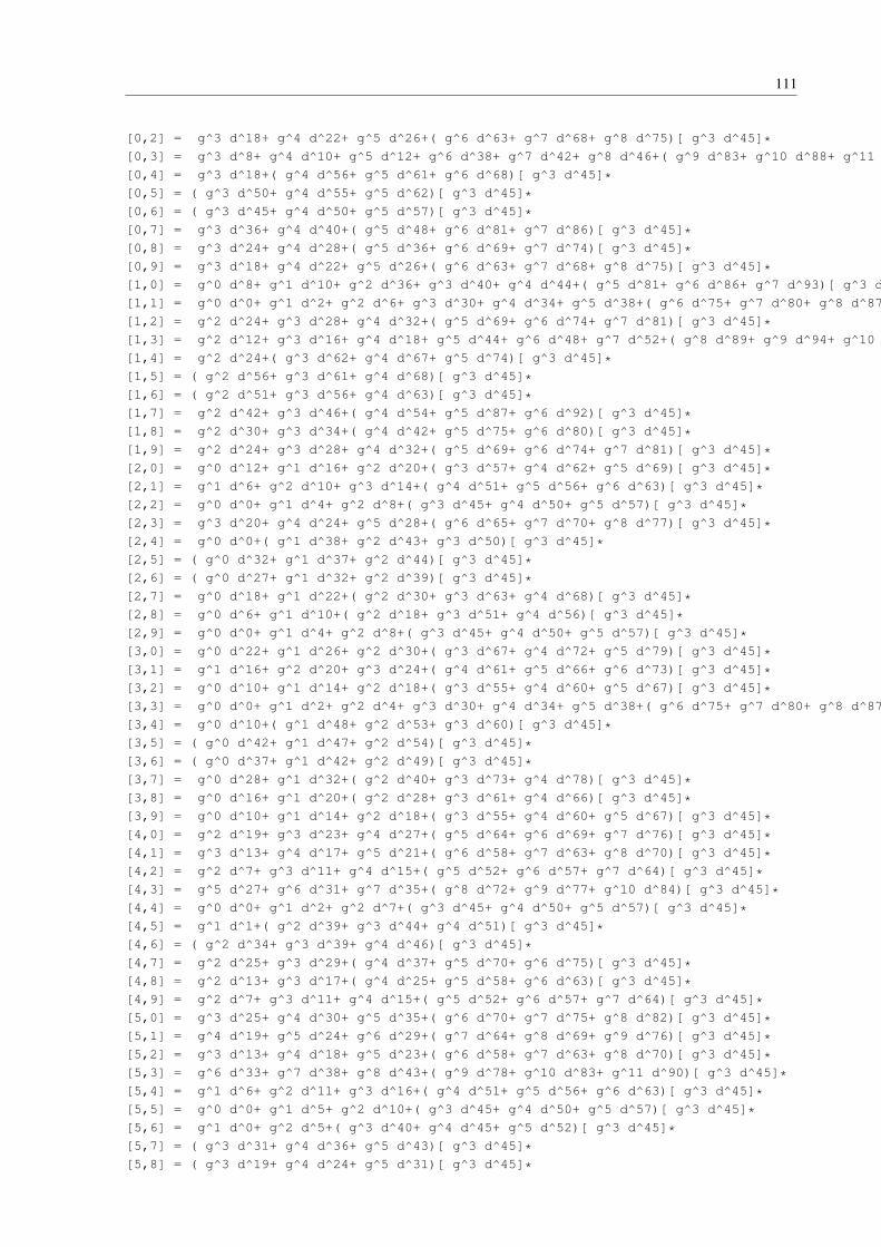
111
[0,2] = g^3 d^18+ g^4 d^22+ g^5 d^26+( g^6 d^63+ g^7 d^68+ g^8 d^75)[ g^3 d^45]*[0,3] = g^3 d^8+ g^4 d^10+ g^5 d^12+ g^6 d^38+ g^7 d^42+ g^8 d^46+( g^9 d^83+ g^10 d^88+ g^11 d^95)[ g^3 d^45]*[0,4] = g^3 d^18+( g^4 d^56+ g^5 d^61+ g^6 d^68)[ g^3 d^45]*[0,5] = ( g^3 d^50+ g^4 d^55+ g^5 d^62)[ g^3 d^45]*[0,6] = ( g^3 d^45+ g^4 d^50+ g^5 d^57)[ g^3 d^45]*[0,7] = g^3 d^36+ g^4 d^40+( g^5 d^48+ g^6 d^81+ g^7 d^86)[ g^3 d^45]*[0,8] = g^3 d^24+ g^4 d^28+( g^5 d^36+ g^6 d^69+ g^7 d^74)[ g^3 d^45]*[0,9] = g^3 d^18+ g^4 d^22+ g^5 d^26+( g^6 d^63+ g^7 d^68+ g^8 d^75)[ g^3 d^45]*[1,0] = g^0 d^8+ g^1 d^10+ g^2 d^36+ g^3 d^40+ g^4 d^44+( g^5 d^81+ g^6 d^86+ g^7 d^93)[ g^3 d^45]*[1,1] = g^0 d^0+ g^1 d^2+ g^2 d^6+ g^3 d^30+ g^4 d^34+ g^5 d^38+( g^6 d^75+ g^7 d^80+ g^8 d^87)[ g^3 d^45]*[1,2] = g^2 d^24+ g^3 d^28+ g^4 d^32+( g^5 d^69+ g^6 d^74+ g^7 d^81)[ g^3 d^45]*[1,3] = g^2 d^12+ g^3 d^16+ g^4 d^18+ g^5 d^44+ g^6 d^48+ g^7 d^52+( g^8 d^89+ g^9 d^94+ g^10 d^101)[ g^3 d^45]*[1,4] = g^2 d^24+( g^3 d^62+ g^4 d^67+ g^5 d^74)[ g^3 d^45]*[1,5] = ( g^2 d^56+ g^3 d^61+ g^4 d^68)[ g^3 d^45]*[1,6] = ( g^2 d^51+ g^3 d^56+ g^4 d^63)[ g^3 d^45]*[1,7] = g^2 d^42+ g^3 d^46+( g^4 d^54+ g^5 d^87+ g^6 d^92)[ g^3 d^45]*[1,8] = g^2 d^30+ g^3 d^34+( g^4 d^42+ g^5 d^75+ g^6 d^80)[ g^3 d^45]*[1,9] = g^2 d^24+ g^3 d^28+ g^4 d^32+( g^5 d^69+ g^6 d^74+ g^7 d^81)[ g^3 d^45]*[2,0] = g^0 d^12+ g^1 d^16+ g^2 d^20+( g^3 d^57+ g^4 d^62+ g^5 d^69)[ g^3 d^45]*[2,1] = g^1 d^6+ g^2 d^10+ g^3 d^14+( g^4 d^51+ g^5 d^56+ g^6 d^63)[ g^3 d^45]*[2,2] = g^0 d^0+ g^1 d^4+ g^2 d^8+( g^3 d^45+ g^4 d^50+ g^5 d^57)[ g^3 d^45]*[2,3] = g^3 d^20+ g^4 d^24+ g^5 d^28+( g^6 d^65+ g^7 d^70+ g^8 d^77)[ g^3 d^45]*[2,4] = g^0 d^0+( g^1 d^38+ g^2 d^43+ g^3 d^50)[ g^3 d^45]*[2,5] = ( g^0 d^32+ g^1 d^37+ g^2 d^44)[ g^3 d^45]*[2,6] = ( g^0 d^27+ g^1 d^32+ g^2 d^39)[ g^3 d^45]*[2,7] = g^0 d^18+ g^1 d^22+( g^2 d^30+ g^3 d^63+ g^4 d^68)[ g^3 d^45]*[2,8] = g^0 d^6+ g^1 d^10+( g^2 d^18+ g^3 d^51+ g^4 d^56)[ g^3 d^45]*[2,9] = g^0 d^0+ g^1 d^4+ g^2 d^8+( g^3 d^45+ g^4 d^50+ g^5 d^57)[ g^3 d^45]*[3,0] = g^0 d^22+ g^1 d^26+ g^2 d^30+( g^3 d^67+ g^4 d^72+ g^5 d^79)[ g^3 d^45]*[3,1] = g^1 d^16+ g^2 d^20+ g^3 d^24+( g^4 d^61+ g^5 d^66+ g^6 d^73)[ g^3 d^45]*[3,2] = g^0 d^10+ g^1 d^14+ g^2 d^18+( g^3 d^55+ g^4 d^60+ g^5 d^67)[ g^3 d^45]*[3,3] = g^0 d^0+ g^1 d^2+ g^2 d^4+ g^3 d^30+ g^4 d^34+ g^5 d^38+( g^6 d^75+ g^7 d^80+ g^8 d^87)[ g^3 d^45]*[3,4] = g^0 d^10+( g^1 d^48+ g^2 d^53+ g^3 d^60)[ g^3 d^45]*[3,5] = ( g^0 d^42+ g^1 d^47+ g^2 d^54)[ g^3 d^45]*[3,6] = ( g^0 d^37+ g^1 d^42+ g^2 d^49)[ g^3 d^45]*[3,7] = g^0 d^28+ g^1 d^32+( g^2 d^40+ g^3 d^73+ g^4 d^78)[ g^3 d^45]*[3,8] = g^0 d^16+ g^1 d^20+( g^2 d^28+ g^3 d^61+ g^4 d^66)[ g^3 d^45]*[3,9] = g^0 d^10+ g^1 d^14+ g^2 d^18+( g^3 d^55+ g^4 d^60+ g^5 d^67)[ g^3 d^45]*[4,0] = g^2 d^19+ g^3 d^23+ g^4 d^27+( g^5 d^64+ g^6 d^69+ g^7 d^76)[ g^3 d^45]*[4,1] = g^3 d^13+ g^4 d^17+ g^5 d^21+( g^6 d^58+ g^7 d^63+ g^8 d^70)[ g^3 d^45]*[4,2] = g^2 d^7+ g^3 d^11+ g^4 d^15+( g^5 d^52+ g^6 d^57+ g^7 d^64)[ g^3 d^45]*[4,3] = g^5 d^27+ g^6 d^31+ g^7 d^35+( g^8 d^72+ g^9 d^77+ g^10 d^84)[ g^3 d^45]*[4,4] = g^0 d^0+ g^1 d^2+ g^2 d^7+( g^3 d^45+ g^4 d^50+ g^5 d^57)[ g^3 d^45]*[4,5] = g^1 d^1+( g^2 d^39+ g^3 d^44+ g^4 d^51)[ g^3 d^45]*[4,6] = ( g^2 d^34+ g^3 d^39+ g^4 d^46)[ g^3 d^45]*[4,7] = g^2 d^25+ g^3 d^29+( g^4 d^37+ g^5 d^70+ g^6 d^75)[ g^3 d^45]*[4,8] = g^2 d^13+ g^3 d^17+( g^4 d^25+ g^5 d^58+ g^6 d^63)[ g^3 d^45]*[4,9] = g^2 d^7+ g^3 d^11+ g^4 d^15+( g^5 d^52+ g^6 d^57+ g^7 d^64)[ g^3 d^45]*[5,0] = g^3 d^25+ g^4 d^30+ g^5 d^35+( g^6 d^70+ g^7 d^75+ g^8 d^82)[ g^3 d^45]*[5,1] = g^4 d^19+ g^5 d^24+ g^6 d^29+( g^7 d^64+ g^8 d^69+ g^9 d^76)[ g^3 d^45]*[5,2] = g^3 d^13+ g^4 d^18+ g^5 d^23+( g^6 d^58+ g^7 d^63+ g^8 d^70)[ g^3 d^45]*[5,3] = g^6 d^33+ g^7 d^38+ g^8 d^43+( g^9 d^78+ g^10 d^83+ g^11 d^90)[ g^3 d^45]*[5,4] = g^1 d^6+ g^2 d^11+ g^3 d^16+( g^4 d^51+ g^5 d^56+ g^6 d^63)[ g^3 d^45]*[5,5] = g^0 d^0+ g^1 d^5+ g^2 d^10+( g^3 d^45+ g^4 d^50+ g^5 d^57)[ g^3 d^45]*[5,6] = g^1 d^0+ g^2 d^5+( g^3 d^40+ g^4 d^45+ g^5 d^52)[ g^3 d^45]*[5,7] = ( g^3 d^31+ g^4 d^36+ g^5 d^43)[ g^3 d^45]*[5,8] = ( g^3 d^19+ g^4 d^24+ g^5 d^31)[ g^3 d^45]*

112 APPENDIX A. Transfer Function and Controllers
[5,9] = g^3 d^13+ g^4 d^18+ g^5 d^23+( g^6 d^58+ g^7 d^63+ g^8 d^70)[ g^3 d^45]*[6,0] = g^3 d^30+ g^4 d^35+ g^5 d^40+( g^6 d^75+ g^7 d^80+ g^8 d^87)[ g^3 d^45]*[6,1] = g^4 d^24+ g^5 d^29+ g^6 d^34+( g^7 d^69+ g^8 d^74+ g^9 d^81)[ g^3 d^45]*[6,2] = g^3 d^18+ g^4 d^23+ g^5 d^28+( g^6 d^63+ g^7 d^68+ g^8 d^75)[ g^3 d^45]*[6,3] = g^6 d^38+ g^7 d^43+ g^8 d^48+( g^9 d^83+ g^10 d^88+ g^11 d^95)[ g^3 d^45]*[6,4] = g^1 d^11+ g^2 d^16+ g^3 d^21+( g^4 d^56+ g^5 d^61+ g^6 d^68)[ g^3 d^45]*[6,5] = g^0 d^5+ g^1 d^10+ g^2 d^15+( g^3 d^50+ g^4 d^55+ g^5 d^62)[ g^3 d^45]*[6,6] = g^0 d^0+ g^1 d^5+ g^2 d^10+( g^3 d^45+ g^4 d^50+ g^5 d^57)[ g^3 d^45]*[6,7] = g^2 d^0+( g^3 d^36+ g^4 d^41+ g^5 d^48)[ g^3 d^45]*[6,8] = ( g^3 d^24+ g^4 d^29+ g^5 d^36)[ g^3 d^45]*[6,9] = g^3 d^18+ g^4 d^23+ g^5 d^28+( g^6 d^63+ g^7 d^68+ g^8 d^75)[ g^3 d^45]*[7,0] = ( g^3 d^39+ g^4 d^44+ g^5 d^51)[ g^3 d^45]*[7,1] = ( g^4 d^33+ g^5 d^38+ g^6 d^45)[ g^3 d^45]*[7,2] = ( g^3 d^27+ g^4 d^32+ g^5 d^39)[ g^3 d^45]*[7,3] = ( g^6 d^47+ g^7 d^52+ g^8 d^59)[ g^3 d^45]*[7,4] = ( g^1 d^20+ g^2 d^25+ g^3 d^32)[ g^3 d^45]*[7,5] = ( g^0 d^14+ g^1 d^19+ g^2 d^26)[ g^3 d^45]*[7,6] = ( g^0 d^9+ g^1 d^14+ g^2 d^21)[ g^3 d^45]*[7,7] = g^0 d^0+ g^1 d^2+( g^2 d^12+ g^3 d^45+ g^4 d^50)[ g^3 d^45]*[7,8] = ( g^2 d^0+ g^3 d^33+ g^4 d^38)[ g^3 d^45]*[7,9] = ( g^3 d^27+ g^4 d^32+ g^5 d^39)[ g^3 d^45]*[8,0] = g^2 d^12+( g^3 d^51+ g^4 d^56+ g^5 d^63)[ g^3 d^45]*[8,1] = g^3 d^6+( g^4 d^45+ g^5 d^50+ g^6 d^57)[ g^3 d^45]*[8,2] = g^2 d^0+( g^3 d^39+ g^4 d^44+ g^5 d^51)[ g^3 d^45]*[8,3] = g^5 d^20+( g^6 d^59+ g^7 d^64+ g^8 d^71)[ g^3 d^45]*[8,4] = ( g^1 d^32+ g^2 d^37+ g^3 d^44)[ g^3 d^45]*[8,5] = ( g^0 d^26+ g^1 d^31+ g^2 d^38)[ g^3 d^45]*[8,6] = ( g^0 d^21+ g^1 d^26+ g^2 d^33)[ g^3 d^45]*[8,7] = g^0 d^12+ g^1 d^14+( g^2 d^24+ g^3 d^57+ g^4 d^62)[ g^3 d^45]*[8,8] = g^0 d^0+ g^1 d^2+( g^2 d^12+ g^3 d^45+ g^4 d^50)[ g^3 d^45]*[8,9] = g^2 d^0+( g^3 d^39+ g^4 d^44+ g^5 d^51)[ g^3 d^45]*[9,0] = g^0 d^12+ g^1 d^16+ g^2 d^20+( g^3 d^57+ g^4 d^62+ g^5 d^69)[ g^3 d^45]*[9,1] = g^1 d^6+ g^2 d^10+ g^3 d^14+( g^4 d^51+ g^5 d^56+ g^6 d^63)[ g^3 d^45]*[9,2] = g^0 d^0+ g^1 d^4+ g^2 d^8+( g^3 d^45+ g^4 d^50+ g^5 d^57)[ g^3 d^45]*[9,3] = g^3 d^20+ g^4 d^24+ g^5 d^28+( g^6 d^65+ g^7 d^70+ g^8 d^77)[ g^3 d^45]*[9,4] = g^0 d^0+( g^1 d^38+ g^2 d^43+ g^3 d^50)[ g^3 d^45]*[9,5] = ( g^0 d^32+ g^1 d^37+ g^2 d^44)[ g^3 d^45]*[9,6] = ( g^0 d^27+ g^1 d^32+ g^2 d^39)[ g^3 d^45]*[9,7] = g^0 d^18+ g^1 d^22+( g^2 d^30+ g^3 d^63+ g^4 d^68)[ g^3 d^45]*[9,8] = g^0 d^6+ g^1 d^10+( g^2 d^18+ g^3 d^51+ g^4 d^56)[ g^3 d^45]*[9,9] = g^0 d^0+ g^1 d^4+ g^2 d^8+( g^3 d^45+ g^4 d^50+ g^5 d^57)[ g^3 d^45]*