modeling technique for the efficient design of microwave

HAL Id: tel-01421150https://hal.archives-ouvertes.fr/tel-01421150

Submitted on 21 Dec 2016

HAL is a multi-disciplinary open accessarchive for the deposit and dissemination of sci-entific research documents, whether they are pub-lished or not. The documents may come fromteaching and research institutions in France orabroad, or from public or private research centers.

L’archive ouverte pluridisciplinaire HAL, estdestinée au dépôt et à la diffusion de documentsscientifiques de niveau recherche, publiés ou non,émanant des établissements d’enseignement et derecherche français ou étrangers, des laboratoirespublics ou privés.

Modeling technique for the efficient design of microwavebandpass filtersMatthias Caenepeel

To cite this version:Matthias Caenepeel. Modeling technique for the efficient design of microwave bandpass filters. Engi-neering Sciences [physics]. INRIA Sophia Antipolis - Méditerranée; Vrije Universiteit Brussels, 2016.English. tel-01421150

https://hal.archives-ouvertes.fr/tel-01421150

https://hal.archives-ouvertes.fr

UNIVERSITE DE NICE-SOPHIA ANTIPOLIS

ECOLE DOCTORALE STIC SCIENCES ET TECHNOLOGIES DE L’INFORMATION ET DE LA COMMUNICATION

T H E S E

pour l’obtention du grade de

Docteur en Sciences

de l’Université de Nice-Sophia Antipolis

présentée et soutenue par

AUTEUR Matthias CAENEPEEL Modeling technique for the efficient design of microwave bandpass

filters

Thèse dirigée par Yves ROLAIN et Martine Olivi

soutenue le 19 Octobre 2016 Jury : G. Macciarella Professeur Rapporteur A. Alvarez-Melcón Professeur Rapporteur A. Pérrigaud Ingénieur de recherche Examinateur F. Ferranti Professeur Examinateur A. Hubin Professeur Examinateur R. Vounck Professeur Examinateur Y. Rolain Professeur Directeur de thèse M. Olivi Chargée de recherche Directeur de thèse F. Seyfert Chargé de recherche Co-directeur de thèse

Vrije Universiteit Brussel (VUB) Faculty of engineering (IR)

Department of fundamental electricity and instrumentation (ELEC)

INRIA (Université Nice Sophia Antipolis) Team APICS: Analysis and problems of inverse type in control and signal processing

MODELING TECHNIQUES FOR THE EFFICIENT DESIGN

OF MICROWAVE BANDPASS FILTERS

Thesis submitted in fulfilment of the requirements for the award of the degree of Doctor in Engineering Sciences (Doctor in de ingenieurswetenschappen) by

Matthias Caenepeel

October 2016

Advisors: Prof. dr. ir. Yves Rolain Martine Olivi Chargée de recherche Fabien Seyfert Chargé de recherche

Members of the jury

Prof. dr. ir. Yves Rolain (advisor)

Vrije Universiteit Brussel

Chargee de recherche Martine Olivi (advisor)

INRIA

Charge de recherche Fabien Seyfert (advisor)

INRIA

Prof. dr. ir. Annick Hubin (chairman)


Prof. dr. Roger Vounckx (vice-chairman)


Prof. dr. ir. Alejandro Alvarez-Melcon (rapporteur)

Universidad Politecnica De Cartagena, Spain

Prof. dr. ir. Giuseppe Macchiarella (rapporteur)

Politecnico di Milano, Italy

Prof. dr. ir. Francesco Ferranti (secretary)


dr. ir. Aurelien Perigaud

XLIM, France

i

Acknowledgements

During the last four years I’ve had the opportunity to do a joint PhD between the

ELEC department of the VUB and the APICS team of INRIA Sophia-Antipolis.

This experience broadened my vision on science, engineering and life in general.

I want to thank all of the people that made this possible and supported me

during this unforgettable experience.

First of all I would like to thank Yves Rolain, Martine Olivi and Fabien Seyfert

for their guidance and for giving me the opportunity to do this PhD.

Yves, first of all I would like to thank you for believing in me as a PhD candidate.

By pushing me out of my comfort zone, you have helped me to develop several

skills. Your enthusiastic way of teaching has taught me the importance of a

well-structured yet vivid presentation. I also want to thank you for correcting

my writings. Although the result of these corrections was not always pleasant,

it has drastically improved my writing skills. Finally I would like to thank you

for the all the interesting discussions we had during the last five years, not only

on technical subjects but also on other topics. I am proud to say that I have

been one of your PhD students.

Martine, first of all thank you for helping me set up this joint PhD. I also highly

appreciated your patience when you were explaining me various mathematical

concepts and helping me with proofs. I would also like to thank you for always

thoroughly reading my writings. Your eye for detail is truly remarkable. Finally

I want to thank you for always helping me to put things into perspective when

I thought everything was going in the wrong direction.

Fabien, thank you for all of the hours you have invested in discussing about and

explaining me the coupling matrix theory. Thank you for the late evenings you

spent with me at INRIA and for the Skype meetings to figure out the errors in my

work. Although I lacked the energy to figure out an important error at the end

iii

of my thesis, I am really glad you have pushed me to do so. Moreover you have

convinced me that scientific results are more important than writing astronomic

amounts of papers. Your view on life, critical attitude towards results and sense

of humor have truly inspired me.

Next, I would like to thank Annick Hubin, Roger Vounckx, Francesco Ferranti,

Aurelien Perigaud, Giuseppe Macchiarella and Alejandro Alvarez-Melcon for

being a member of the jury of my thesis. Your comments, questions and expertise

allowed me to drastically improve the quality of this work.

Also I would like to thank both of the research teams APICS and ELEC for

providing a pleasant environment and all the necessary means to be able to

do my research. I would especially like to thank Ann Pintelon, Johan Pattyn,

Stephanie Sorres and Sven Reyniers for all of their administrative and technical

support.

During my PhD I have also learned the value of collegiality and friendship. I

was very lucky to share an office with Hannes, Adam and Egon at ELEC.

Hannes, you are a true friend to whom I can talk about literally every aspect of

my life. Thank you for all the support, advice and good times we had. I strongly

value your opinion. Your view on things has helped me clear my mind several

times. Moreover our trip the USA was one of the best experiences of my life. I

am really going to miss seeing you on a daily basis.

Adam, working on a project or traveling together with you always has brought

us closer as friends. Thank you for solving all those questions I was struggling

with. I truly hope that our professional paths will cross again in the future. But

for now I wish you all the best as a new member of the APICS team.

Egon, I am glad that we did not only share an office but that we also worked

together on the ping-pong tower project. You are one of the most helpful people

I know. I would specifically like to thank you for all of the times you helped me

with computer related issues.

I would also like to thank Maral and Evi for working together with me on

microwave filters. Maral, due to the topic of your master thesis, you pushed this

work in the direction of the coupling matrix theory. This would not have been

the same work if it wasn’t for you.

I would also like to thank Francesco and Krishnan for working with me on

incorporating metamodels in filter design. Francesco, I thank you for sharing

your expertise with me. It was a real pleasure to work with you.

iv

I would also like to thank Piet, Ebrahim, Dries, John, Anna, Maarten, Jan,

Alexander, Cedric, Koen, Philippe, Rik, Gerd and Leo for being such nice col-

leagues. Thank you for all of the nice chats and laughter during several lunches,

coffee breaks and beer Fridays. I would specifically like to thank Piet for all the

extra good times he offered me during our daily lifting sessions.

I would also like to thank Glenn and Philemon for living with me during the

first two years of this PhD. Thanks for all whisky tastings, balcony discussions

and crazy times we had in our little palace.

I was very lucky to be part of such warm and pleasant research group at INRIA.

Dmitry, although I called you Vladimir during my first week at INRIA, I will

always remember your name. Your presence made my visits to APICS even

more pleasant. I am also very proud to be a part of the Porco Rosso team:

Christos, Stephano, Konstaninos and Dmitry. I would like to thank you all for

your support, good times and nice food we had together. And a special thanks

for the moral support when my computer crashed while I was writing this thesis.

I would also like to thank David for all the discussions about our works in order

to improve them both. Finally I also want to thank Juliette, Sylvain and Laurent

for the warm welcoming every time I visited.

At the VUB in general, I have always been surrounded by lovely people: Hannes,

Philemon, Glenn, Maarten, Adam, Lara, Petey, Ken, Jens, Hans, Simen and

Aushim. Thank you for all the parties, concerts and crazy nights we had to-

gether. May more of these good times follow in the future!

Another very important person during me PhD is my brother, Free. Having a

beer or a run together always gave me the right energy to push me further into

my research or putting things into perspective when I was having a hard time.

Thank you for your support and I hope I am able to do the same for you.

There are no words to express my love and gratitude towards Evy. Thank you

for always being there for me. I highly appreciate your open mind towards my

long stays in France. I would also like to thank you for your contributions to

the visual aspects of my work in general. Without you, the layout of this thesis

would simply have been ugly. Finally I want to thank you for your patience,

especially during the last days of the writing period. Evy, thank you for all of

the help, support, freedom and love you have been given me during this PhD.

v

Finally I want to thank my parents for all of the opportunities and the beautiful

youth they have given me. Papa, sending me to the VUB is one of the best

things that ever happened to me. Mama, it is impossible to list up all of the

amazing things you have done for me over the last 27 years.

Therefore I would like to dedicate this work to my parents.

Matthias Caenepeel

Antibes and Brussels, October 2016

vi

Abstract

The design of microwave bandpass filter generally requires optimization or fine-

tuning of the physical design parameters in order to meet the electrical spec-

ifications given by a frequency template. In this thesis we develop models to

assist the designer in the time-efficient physical design of the distributed ele-

ment microwave filters. The aim is to incorporate these models in different

computer-aided design (CAD) methods. By a time-efficient design, we mean

a design that requires a low number of electromagnetic (EM) simulations. The

EM-simulations typically represent the most time-consuming step during the op-

timization process. We propose different modeling approaches for the frequency

response behavior of the filter. The first approach models the coupling matrix

as a function of the physical design parameters and the second approach models

the scattering (S-) parameters, again as a function of the physical parameters.

In the first part of the text we focus on the design of narrow-band microwave

bandpass filters implemented in a microstrip technology. The design of such

filters is often based on the coupling matrix theory. It models the distributed

element microwave filter by a lumped element circuit consisting of coupled LC-

resonators that resonate in the vicinity of its center frequency. The behavior of

these coupled resonator circuits is represented by a coupling matrix. The first

step of the design process synthesizes a coupling matrix (golden goal) realizing a

filter function that fulfills the frequency specifications. Next this coupling matrix

is physically implemented by correctly dimensioning the design parameters of

the actual microwave filter. Over the last few years several computer-aided

tuning (CAT) methods have been developed to optimize the physical design

parameters. These tuning methods often extract a coupling matrix from the

filters S-parameters and compare it to the golden goal. The extraction of the

coupling matrix is critical, especially in the case of coupling topologies that allow

multiple solutions.

vii

Therefore we have developed a coupling matrix extraction procedure that identi-

fies the physically implemented coupling matrix. Moreover we introduce a novel

CAT technique based on an efficient estimation of the Jacobian of the func-

tion relating the design parameters to the (physical) coupling parameters. The

estimation of the Jacobian uses adjoint sensitivity analysis , which drastically

reduces the number of required EM-simulations. This novel technique has been

applied to design examples having multiple-solution coupling topologies.

In the second part of the thesis we propose an alternative modeling approach

which is a based on the concept of a metamodel. The idea is that the metamodel

is numerically much cheaper to evaluate than the original simulation model

while keeping an acceptable accuracy. First we use the metamodel approach to

efficiently generate initial values for the filters’ physical design parameters. Next

we will use metamodels to optimize the S-parameters. The use of metamodels

reduces the time required to optimize the filters heavily. Moreover metamodels

can be used to optimize for different design scenarios.

viii

Contents

Members of the jury i

Acknowledgements iii

Abstract vii

Contents xi

List of symbols xiii

1 Introduction 1

I Coupling Matrix Approach 7

2 Narrow-band Bandpass Filter Design based on Coupling Matrix Theory 9

2.1 Introduction . . . . . . . . . . . . . . . . . . . . . . . . . . . . . . 9

2.2 Rational Form of the Scattering Parameters . . . . . . . . . . . . 11

2.3 The Pseudo-elliptical Filter Function . . . . . . . . . . . . . . . . 16

2.4 Equivalent Lumped Bandpass Network . . . . . . . . . . . . . . . 21

2.5 Equivalent Lumped Lowpass Network . . . . . . . . . . . . . . . 23

2.6 Coupling Matrix Representation . . . . . . . . . . . . . . . . . . 28

2.7 Synthesis of the Coupling Matrix . . . . . . . . . . . . . . . . . . 36

2.8 Reconfiguration of the Coupling Matrix . . . . . . . . . . . . . . 44

3 Physical Implementation of the Coupling Matrix in Microstrip Technology 51

3.1 Introduction . . . . . . . . . . . . . . . . . . . . . . . . . . . . . . 51

3.2 Microstrip Structure . . . . . . . . . . . . . . . . . . . . . . . . . 53

3.3 Half-Wavelength (λ2 ) Resonators . . . . . . . . . . . . . . . . . . 56

3.4 Electromagnetic (EM-) Simulators . . . . . . . . . . . . . . . . . 58

3.5 Generation of the Design Curves . . . . . . . . . . . . . . . . . . 59

3.6 Initial Dimensioning of a Single Quadruplet SOLR Filter . . . . . 70

3.7 Conclusion . . . . . . . . . . . . . . . . . . . . . . . . . . . . . . 73

ix

4 Extraction of the Coupling Matrix 75

4.1 Introduction . . . . . . . . . . . . . . . . . . . . . . . . . . . . . . 75

4.2 Bandpass-to-Lowpass Transformation . . . . . . . . . . . . . . . 79

4.3 Rational Approximation and Reference Plane Adjustment of the

S-parameters . . . . . . . . . . . . . . . . . . . . . . . . . . . . . 79

4.4 Synthesis of the Coupling Matrix in Arrow Form . . . . . . . . . 85

4.5 Reconfiguration of the Extracted Arrow Form Matrix . . . . . . 86

4.6 Dealing with Parasitic Couplings . . . . . . . . . . . . . . . . . . 88

4.7 Example: Single Quadruplet (SQ) Filter . . . . . . . . . . . . . . 90

4.8 Example: Cascaded Quadruplet (CQ) Filter . . . . . . . . . . . . 97

4.9 Conclusion . . . . . . . . . . . . . . . . . . . . . . . . . . . . . . 104

5 Dealing with Multiple Solutions: A Simulation Based Strategy 107

5.1 Introduction . . . . . . . . . . . . . . . . . . . . . . . . . . . . . . 107

5.2 Cascaded Trisection and Quadruplet Topologies . . . . . . . . . . 108

5.3 Identification of the Physically Implemented Coupling Matrix . . 112

5.4 Tuning of a CQ filter . . . . . . . . . . . . . . . . . . . . . . . . . 117

5.5 Conclusion . . . . . . . . . . . . . . . . . . . . . . . . . . . . . . 126

6 Electromagnetic Optimization of Microstrip Bandpass Filters based on Ad-

joint Sensitivity Analysis 127

6.1 Introduction . . . . . . . . . . . . . . . . . . . . . . . . . . . . . . 127

6.2 Adjoint Sensitivity of the S-parameters with respect to the Cou-

pling Parameters . . . . . . . . . . . . . . . . . . . . . . . . . . . 129

6.3 Estimation of the Jacobian Matrix J . . . . . . . . . . . . . . . . 131

6.4 Determination of the Physically Implemented Coupling Matrix . 134

6.5 Re-optimization of the Target Coupling Matrix . . . . . . . . . . 134

6.6 Tuning Method . . . . . . . . . . . . . . . . . . . . . . . . . . . . 136

6.7 Tuning of a CT filter . . . . . . . . . . . . . . . . . . . . . . . . . 138

6.8 Tuning of a SQ filter . . . . . . . . . . . . . . . . . . . . . . . . . 149

6.9 Discussion . . . . . . . . . . . . . . . . . . . . . . . . . . . . . . . 153

6.10 Remarks . . . . . . . . . . . . . . . . . . . . . . . . . . . . . . . . 154

6.11 Conclusion . . . . . . . . . . . . . . . . . . . . . . . . . . . . . . 154

II Metamodel Approach 157

7 Efficient and Automated Generation of Multidimensional Design Curves

using Metamodels 159

7.1 Introduction . . . . . . . . . . . . . . . . . . . . . . . . . . . . . . 159

7.2 Generation of the Design Curves using Metamodels . . . . . . . . 161

7.3 Example: Hairpin Resonator Filter . . . . . . . . . . . . . . . . . 164

x

7.4 Conclusion . . . . . . . . . . . . . . . . . . . . . . . . . . . . . . 170

8 A Scalable Macromodeling Methodology for the Efficient Design of Mi-

crowave Filters 171

8.1 Introduction . . . . . . . . . . . . . . . . . . . . . . . . . . . . . . 171

8.2 Scalable Macromodels for Microwave Filters . . . . . . . . . . . . 173

8.3 Including the Scalable Macromodel in the Design Process . . . . 177

8.4 Macromodel based Optimization . . . . . . . . . . . . . . . . . . 178

8.5 Example: Microstrip Dual-Band Bandpass Filter . . . . . . . . . 179

8.6 Discussion . . . . . . . . . . . . . . . . . . . . . . . . . . . . . . . 187

8.7 Conclusion . . . . . . . . . . . . . . . . . . . . . . . . . . . . . . 191

Conclusions 193

9 Conclusions 195

9.1 Comparison of the proposed approaches . . . . . . . . . . . . . . 197

9.2 Main contributions . . . . . . . . . . . . . . . . . . . . . . . . . . 199

10 Preliminary Results and Future Work 201

10.1 Preliminary Results: Parametric Modeling of the Coupling Pa-

rameters . . . . . . . . . . . . . . . . . . . . . . . . . . . . . . . . 201

10.2 Future Work . . . . . . . . . . . . . . . . . . . . . . . . . . . . . 202

List of scientific publications 205

Appendices 207

A Appendix A 209

xi

List of symbols

LATIN LOWER CASE

ai transmitted power wave at port i

bi reflected power wave at port i

c phase velocity in free space ( c ≈ 3× 108 ms )

f frequency

fc center frequency in the bandpass domain

fres resonance frequency

j unit imaginary number , j2 = −1

ks filter selectivity

kX bandpass inter-resonator coupling coefficient

kB mixed bandpass coupling coefficient

kE electric bandpass coupling coefficient

kM magnetic bandpass coupling coefficient

h thickness of the dielectric substrate of a microstrip structure

l physical length of a transmission line

nF number of simulated frequencies

nfz number of transmission zeros located at a finite frequency

ng number of physical design parameters

nS number of solutions to the coupling matrix reconfiguration

problem

s Laplace variable, s = σ + jω

t thickness of metal strip of a microstrip structure

LATIN UPPER CASE

ALP nodal admittance matrix in the lowpass domain

ABP nodal admittance matrix in the bandpass

AY system matrix of the admittance matrix Y

BY input matrix of the admittance matrix Y

CY output matrix of the admittance matrix Y

xiii

DY direct transmission matrix of the admittance matrix Y

BW absolute bandwidth

Ca per unit capacitance for air

Cd per unit capacitance for a dielectric

E(s) common denominator polynomial

F (s) numerator polynomial of S11(s)

FBW fractional or relative bandwidth

GL reference admittance at the load

GS reference admittance at the source

In identity matrix of size n× nJ Jacobian matrix of the function that maps the geometrical

parameters to the coupling parameters

J J-inverter

KN filter function of order N

LA insertion loss

LR return loss

Mvv lowpass self-coupling of resonator v

Marr arrow form coupling matrix

N McMillan degree

P similarity transformation

P (s) numerator polynomial of S21(s)

Qc conductor quality factor

Qd dielectric quality factor

Qe external quality factor

Qr radiation quality factor

Qu unloaded quality factor of a resonator

Qr radiation quality factor

RL minimal return loss in the passband

S scattering matrix

SC scattering matrix with de-embedded access lines

SSim simulated scattering matrix

Srat rational scattering matrix

T coupling topology matrix

W width of metal strip of a microstrip structure

Y admittance matrix

Zc characteristic impedance

ZL reference impedance at the load

ZS reference impedance at the source

xiv

GREEK CASE

α attenuation constant

β lossless propagation constant

αkk delay introduced by the access line at port k

εr relative permittivity

εre effective dielectric constant

γ propagation constant

λ0 wavelength in free space

λg guided wavelength

tan δ loss tangent of a dielectric substrate

τ group delay

θ electrical length

ω normalized angular lowpass frequency

Ω angular bandpass frequency

Ωk resonance frequency of resonator k in the lowpass domain

Ωc center frequency in the lowpass domain

ABBREVIATIONS

AFS adaptive frequency sampling

BP bandpass

CAT computer-aided tuning

CQ cascaded quadruplet

CT cascaded triplet

dB decibels (20 log10)

EM electromagnetic

FIR frequency invariant reactance

FRF frequency response function

I/O input/output

LP lowpass

LSE least square estimation

MAE mean absolute error

MoM method of moments

PCB printed circuit board

SOLR square open loop resonator

SQ single quadruplet

TEM transverse electromagnetic

TZ transmission zero

VF vector fitting

xv

1Introduction

Microwave filters are indispensable building blocks in modern telecommunica-

tion systems. They are designed to pass electromagnetic signals within certain

frequency bands, while attenuating signals whose spectral content lies outside of

these frequency bands. Over the last years the frequency spectrum has become

more and more crowded, which automatically led to more stringent filter spec-

ifications. These specifications consist of a frequency template, which specifies

the frequency bands that should be attenuated and passed. Several techniques

have been developed to design a wide variety of microwave filters in various

technologies such as: waveguide, dielectric resonator and planar technologies

such as microstrip filters. The literature helps filter designers to select the most

convenient type of filter to meet the design requirements [Levy 02; Levy 84].

Besides the electrical specifications of the filter, that are grouped in the fre-

quency template, there are several aspects that must be taken into account such

as minimization of the mass and volume, manufacturing cost, development time

and power handling capability [Snyd 07; Kuds 92]. All these aspects influence

both the choice of the implementation technology and of the topology of the

filter to be designed. In this work we focus on the electrical specifications of the

filters. The most common design approach which is also used here, can roughly

be divided into three design stages [Matt 64]:

1. The first stage approximates or estimates a filter function that fulfills the

electrical specifications.

2. The second stage synthesizes an equivalent lumped-element network that

realizes the filter function.

3. The third stage transforms this network into the actual microwave filter

by correctly dimensioning the physical (design) parameters of the filter.

1

In this thesis we focus on the last stage of the design approach. We develop mod-

els to assist the designer in the time-efficient physical design of the distributed

element microwave filters. The aim is to incorporate these models in different

computer-aided design (CAD) methods. By a time-efficient design, we mean a

design that requires a low number of electromagnetic (EM) simulations. The

EM-simulations typically represent the most time-consuming step during the

last design stage. We propose different modeling approaches for the frequency

response behavior of the filter. The first approach models the coupling matrix

(which is introduced later) as a function of the physical design parameters and

the second approach models the scattering (S-) parameters, again as a function

of the physical parameters.

In the first part of the text we focus on the design of narrow-band microwave

bandpass filters implemented in a microstrip technology. The design of such

filters is often based on the coupling matrix theory. It models the distributed

element microwave filter by a lumped element circuit consisting of coupled LC-

resonators that resonate in the vicinity of its center frequency [Hong 01]. The

behavior of these coupled resonator circuits is represented by a coupling matrix

[Came 99; Atia 71]. This matrix contains the electromagnetic couplings between

the different resonators in the filter. The way these resonators are coupled, is

called the coupling topology. The concept of the coupling matrix was first intro-

duced in the early 1970s by Atia and Williams to design a dual-mode symmetric

waveguide filter [Atia 71; Atia 72; Atia 74]. One of its main advantages is that

it can be easily linked to the physical design parameters of the actual filter

[Came 07b].

Chapter 2 explains the concepts of the coupling matrix based design approach

that will be used in the rest of the text: the generation of a rational filter function

and the synthesis of a coupling matrix which represents the equivalent lumped-

element network. In order to translate the coupling matrix into the actual

microwave filter, it is necessary to transform the coupling matrix into a coupling

topology that is adapted to the selected filter structure. This process is often

referred to as the reconfiguration of the coupling matrix. The reconfiguration

problem is a complex problem and for some coupling topologies there are multiple

solutions. Topologies with multiple solutions are called non-canonical topologies.

Several methods have been developed to tackle the reconfiguration problem:

some of them are optimization-based [Amar 00b; Atia 98] and for some other

topologies analytical techniques exist [Tami 05]. The most general approach uses

Groebner basis and homothopy techniques to solve the reconfiguration problem

2 CHAPTER 1 INTRODUCTION

[Came 07a]. This is also the approach used here. The second stage of the design

process thus yields a coupling matrix with a suitable coupling topology. This

matrix is often referred to as the golden goal or the target coupling matrix.

The third stage of the design process is to dimension the physical filter such

that the coupling matrix of the actual filter is as close as possible to the target

matrix. This step is called the physical implementation. It often starts with

the generation of initial values for the design parameters, which are then further

optimized to meet the specifications.

Chapter 3 proposes a method to generate initial values for the physical parame-

ters. Although the method is general for various technologies, we use microstrip

filters to illustrate it. Therefore the chapter first summarizes the most important

characteristics of microstrip transmission lines that are used in the remainder of

the text. We also discuss the use of the full-wave EM field solvers that are used to

simulate the filters, which are ADS Momentum [ADS 14] and CST Microwave

Studio [CST 15]. We briefly describe the properties of both EM-solvers and the

simulation settings used in this work.

The initial dimensioning divides the filter into building blocks consisting of indi-

vidual resonators or pairs of resonators. Next, it dimensions these blocks sepa-

rately and finally merges them to obtain the complete filter. Therefore it is some-

times referred to as the ’divide and conquer strategy’ [Came 07b]. The dimen-

sioning of each individual block uses design curves. These are look-up tables that

relate the physical parameters to the coupling parameters [Pugl 00; Pugl 01].

We explain how the design curves are generated using simulated S-parameters.

This approach yields relatively good initial values for the design. Nevertheless

an optimization or tuning phase is often required to ensure that the filter meets

the specifications.

In the literature several optimization methods are available to tune microwave

filters based on various cost functions [Swan 07a; Band 94b; Arnd 04; Koza 02].

For the coupling matrix based designs, we follow an approach which compares the

golden goal to the coupling matrix of the physical filter as is done in [Lamp 04;

Koza 06]. A very important step in this approach is the extraction of the physical

coupling matrix. This can be a tedious task especially in the case of coupling

topologies supporting multiple solutions.

Chapter 4 presents a method to extract the coupling matrix starting from the

simulated (or measured) S-parameters of the filter. It first estimates a ratio-

nal common denominator matrix for the S-parameters. Next it, synthesizes a

3

coupling matrix starting from this rational approximation using the techniques

explained in Chapter 2. In general the coupling topology of this matrix does

not correspond to the physically implemented coupling topology. Moreover, the

extracted matrix contains parasitic couplings, which are not present in the golden

goal. In the case of non-canonical topologies, the process extracts all possible so-

lutions taking into account the presence of parasitics. This extraction procedures

gives rise to the following question: Which of these solutions corresponds to the

physically implemented one? Answering this is very important for the tuning of

the filter. Using a non-physical solution may lead to wrong adjustments of the

design parameters, hereby destroying the whole tuning procedure. The answer is

however not always obvious and extra information about the physical structure

of the filter is indispensable.

Chapter 5 presents a novel identification method to determine the physically im-

plemented coupling matrix in the case of cascaded trisection (CT) and cascaded

quadruplet (CQ) topologies. These topologies are often used, since they yield

very selective filter responses [Yang 99; Hong 99; Hong 01]. The identification

method basically links specific parts of the coupling matrix to specific parts

of the physical structure. To establish this link, several EM-simulations are

required. The number of required EM-simulations depends of the complexity of

the structure. The usefulness of the identification method is illustrated on the

tuning of an 8th order CQ filter. The tuning is a manual and requires a relatively

large number of EM-simulations. In order to automate the tuning procedure and

minimize the number of EM-simulations, we propose another approach based on

adjoint sensitivity analysis.

Chapter 6 presents a novel computer-aided tuning (CAT) procedure for coupled

resonator microwave bandpass filters. The method is based on the estimation

of the Jacobian of the relation between the geometrical design parameters of

the filter and the physically implemented coupling parameters. The Jacobian

is estimated by combining the adjoint sensitivity of the S-parameters with re-

spect to the coupling parameters on the one hand and the adjoint sensitivity

of the S-parameters with respect to the physical filter design parameters on

the other hand. Lately, commercial EM-simulators such as CST Microwave

Studio [CST 15] provide the adjoint sensitivities of the S-parameters with re-

spect to the geometrical or substrate parameters of the filter without drastically

increasing the simulation time. As a consequence, one EM-simulation suffices

to estimate the Jacobian. In the case of coupling topologies with multiple so-

lutions, the Jacobian is estimated for each solution separately and a criterion

4 CHAPTER 1 INTRODUCTION

is presented to determine the physical solution amongst the candidates. The

Jacobian provides a lot of useful information for the tuning procedure and we

will see that this drastically lowers the number of EM-simulations required to

tune the filter.

In the second part of the thesis we propose an alternative modeling approach

which is a based on the concept of a metamodel. A metamodel is defined in

the literature as: an approximation of the Input/Output (I/O) function that is

defined by the underlying simulation model [Klei 08]. The word meta implies

that we are actually modeling a (simulation) model. The idea is that the model

is cheaper to evaluate than the original simulation model while keeping an ac-

ceptable accuracy. In this work we consider the physical design parameters as

the input parameters of the metamodel. First we use the metamodel approach to

efficiently generate the design curves introduced in Chapter 3 to generate initial

values. In this context the output parameters of the metamodel are the coupling

parameters of the individual building blocks. Next we will use this approach to

optimize the S-parameters. The output in this case are S-parameters and the

inputs are the design parameters and the frequency. In this context we will use

the term scalable or parametric macromodel, rather than metamodel as this is

more commonly used in the literature [Triv 09; Ferr 11; Ferr 12].

Chapter 7 introduces a metamodel approach to automatically generate multi-

dimensional design curves for the initial dimensioning of coupled-resonator fil-

ters. This approach has some advantages: it requires very little user interaction

and adaptive sampling methods [Wang 07] limit the amount of EM-simulations

needed to generate the curve. Design curves can hence cheaply be generated and

used for the initial dimensioning for multiple design scenarios. The curves yield

initial values and an optimization is generally still required.

Chapter 8 introduces a CAD method based on scalable macromodels to model

the S-parameters as a function of the physical design parameters within a well de-

fined, user selected range of values. Similarly as in Chapter 7, adaptive sampling

methods are used to limit the number of required EM-simulations [Chem 14a].

The fact that the scalable macromodel is numerically cheap to evaluate, reduces

the time required to optimize the filters heavily. Moreover if the ranges of the

design parameters are chosen broad enough, the macromodel can be used to

optimize different design scenarios. Remember that broader ranges come how-

ever at the cost of longer generation times for the model. The CAD method is

applied to a state-of-the art dual-band microstrip filer.

5

PART I

Coupling Matrix Approach

7

2Narrow-band Bandpass Filter Design based on Coupling Matrix Theory

This chapter introduces the coupling matrix theory. This theory assumes that

in the vicinity of its center frequency, the distributed element microwave filter

behaves as a lumped-element circuit consisting of coupled LC-resonators The

lumped-equivalent can be represented by a coupling matrix. In this chapter we

explain the synthesis of a coupling matrix for which the corresponding filter re-

sponse fulfills the specifications; moreover we introduce important concepts that

are related to the design methodology. Section 2.2 introduces the scattering

parameters. Section 2.3 introduces the pseudo-elliptical or general Chebyshev

filter functions, which are the filter functions we focus on in this work. Section 2.4

discusses the behavior of the equivalent lumped-element network used to model

the filter in bandpass domain. Section 2.5 explains how the circuit is trans-

formed to the lowpass domain. Section 2.6 shows how a coupling matrix can be

constructed starting from the lowpass equivalent circuit. We show the relation

between the coupling matrix representation and the state-space representation

of the Y -parameters. In Section 2.7 we use this relation to directly synthesize the

coupling matrix starting from the filter function. Finally Section 2.8 discusses

how the coupling matrix can be reconfigured obtain a coupling topology that

can be physically realized.

2.1 Introduction

The design of the microwave filters considered in this work relies on the coupling

matrix theory. This design methodology assumes that in the vicinity of its

center frequency, the distributed element microwave filter behaves as a lumped-

element circuit consisting of coupled LC-resonators [Came 07b; Hong 01]. This

equivalence holds in the frequency band of interest due to the limited relative

bandwidth of the microwave filter. The behavior of these coupled resonator cir-

cuits can also be represented by a coupling matrix. One of the main advantages

9

of the coupling matrix representation is that it can easily be linked to a physical

circuit topology that is capable to realize the actual filter. This chapter discusses

how such a coupling matrix can be synthesized to ensure that the given design

specifications, called the template of the filter, can be met. Moreover, it intro-

duces some important concepts that are related to the design methodology and

are used intensively in the remainder of this text. The physical implementation

of the filters on the other hand is discussed in Chapter 3.

The electrical (design) specifications of a filter are often expressed by a fre-

quency template or spectral mask on the scattering (S-) parameters introduced

in Section 2.2. The design therefore typically starts by the approximation phase

where a filter function is either estimated or obtained from a table to ensure

that the corresponding S-parameters obey the frequency template. In order

to reduce the complexity, the specifications are transformed to the normalized

lowpass domain. In this work, we focus on the class of pseudo-elliptical or general

Chebyshev filter functions [Came 82], which is introduced in Section 2.3. This

class of filter functions has some interesting characteristics such as an equiripple

behavior in the passband and the fact that its response can be asymmetrical

with respect to the center frequency. The aim of this design methodology is to

synthesize a coupling matrix that realizes the chosen the filter function. There

are 2 ways to do this [Came 07b]:

• The first way starts with the synthesis of a lumped-element network that

realizes the requested filter function. Next, it constructs a coupling matrix

starting from the circuit element values of the network.

• The second way synthesizes a coupling matrix directly from the filter func-

tion, without the need for the circuit representation.

In this work we follow the second way, which avoids the synthesis of the lumped-

element circuit. The coupling matrix represents an equivalent lumped-element

circuit used to model the filter behavior in the vicinity of the center frequency.

Section 2.4 introduces the equivalent lumped-element circuit in the bandpass

domain. Section 2.5 explains how the network is transformed to the lowpass do-

main. Moreover it introduces the frequency invariant reactance (FIR) element,

which has a purely imaginary admittance that does not depend on the frequency.

Due to the FIR element the resonators resonate at frequencies different from the

center frequency of the filter. Such filters are called asynchronously tuned filters.

The FIR element is needed to realize frequency responses that are asymmetric

with respect to the center frequency. Section 2.6 shows how a coupling matrix

10 CHAPTER 2 NARROW-BAND BANDPASS FILTER DESIGN BASED ON COUPLING MATRIX THEORY

can be constructed starting from the equivalent circuit. This section also intro-

duces an alternative way to represent the filters frequency response namely the

admittance or (Y -) parameter representation. We show the relation between

the coupling matrix representation and the state-space representation of the Y -

parameters. In Section 2.7 we use this relation to directly synthesize the coupling

matrix starting from the filter function. The link between the coupling matrix

and the state-space representation also shows that the coupling matrix is not

unique. Applying an orthogonal similarity transformation to the coupling ma-

trix preserves the filter frequency response, while it changes the coupling matrix

topology (the way how resonators are coupled to each other). The coupling

matrix synthesis generally results in a full coupling matrix [Came 99; Seyf 07].

It is possible to transform the full coupling matrix to a canonical form such as

the arrow or the folded form. In this work we use the arrow form. Although this

is a canonical form [Seyf 98] (up to sign changes), it is not always practical (and

sometimes impossible) to implement it physically. Similarity transformations

allow to reconfigure the coupling matrix (change the coupling topology) such

that it becomes more practical to implement. Section 2.8 discusses how the

coupling matrix can be reconfigured to obtain a coupling topology that can be

physically realized. There are however limitations: not every filter response can

be implemented by any coupling topology. The link between the filter response

and the coupling topology is also discussed in this section.

2.2 Rational Form of the Scattering Parameters

2.2.1 THE SCATTERING MATRIX S

We represent the filter by a two-port network as is shown in Figure 2.1, where v1,

v2 and i1, i2 are the port voltages and port currents at port 1 and 2 respectively,

ZS and ZL are the reference impedances at port 1 and 2 respectively and eS

and eL is the source voltages at port 1 and 2 respectively. If we assume that the

reference impedances are real-valued, the transmitted and reflected powerwaves

at port 1 and 2 respectively are defined by [Kuro 65; Mark 92]:

2.2 RATIONAL FORM OF THE SCATTERING PARAMETERS 11

a1 =v1 + ZSi1

2√ZS

b1 =v1 − ZSi1

2√ZS

(2.1)

a2 =v2 + ZLi2

2√ZL

b2 =v2 − ZLi2

2√ZL

(2.2)

The scattering (S-) parameters relate the power waves at the two ports:

S11 =b1a1

∣∣∣∣a2=0

S12 =b1a2

∣∣∣∣a1=0

(2.3)

S21 =b2a1

∣∣∣∣a2=0

S22 =b2a2

∣∣∣∣a1=0

(2.4)

where a1 = 0 when eL 6= 0, eS = 0 and a2 = 0 when eS 6= 0, eL = 0 imply a

perfect match at port 1 and 2 respectively. Since the two-port system is linear

time-invariant, the S-parameters are also frequency dependent. S11 and S22 are

called the reflection coefficients and S12 and S21 the transmission coefficients.

The S-parameters can also be grouped in the scattering (S-) matrix S:

[b1

b2

]=

[S11 S12

S21 S22

][a1

a2

](2.5)

Figure 2.1 The two-port representation of the filter.

Remark that when the two-port is excited by a current source (Figure 2.2) where

GS and GL are the reference admittances and iS is the source current, the waves

become


a1 =GSv1 + i1

2√GS

b1 =GSv1 − i1

2√GS

(2.6)

a2 =GLv2 + i2

2√GL

b2 =GLv2 − i2

2√GL

(2.7)

2-port

Figure 2.2 The two-port representation of the filter excited by a current source.

2.2.2 ABCD-PARAMETERS

Sometimes it is convenient to represent the two-port by means of a cascadable

formalism, to obtain that a tandem connection boils down to a matrix product.

This is done using the ABCD-parameters or ABCD-matrix, which relate the

current and voltage at port 2 to the current and voltage at port 1 in the following

way [Poza 98]:

[v1

i1

]=

[A B

C D

][v2

−i2

](2.8)

where

A =v1

v2

∣∣∣∣i2=0

B =v1

i2

∣∣∣∣v2=0

(2.9)

C =i1v2

∣∣∣∣i2=0

D = − i1i2

∣∣∣∣v2=0

(2.10)

This representation is used to describe the behavior of J-inverters introduced in

Section 2.4.


2.2.3 FILTER SPECIFICATIONS

The design of a bandpass filter starts with frequency dependent specifications

given on the amplitude and sometimes phase of the scattering parameters S11

and S21. A template imposes a maximum amount of reflection in the passband

and a minimum amount of attenuation in the stopbands (Figure 2.3). There, Ω

is the angular frequency in the bandpass domain. In the remainder of this work,

we will call the angular frequency just frequency for the ease of the reader and

the notation. The passband is defined by the lower and upper corner frequency

Ω1 and Ω2. The absolute bandwidth of the filter is BW = Ω2 −Ω1. The center

frequency of the filter is defined by Ω0 = Ω2+Ω1

2 . The fractional bandwidth is

then defined by FBW = Ω2−Ω1

Ω0. A microwave bandpass filter is considered to be

a narrow-band filter when its FBW is less than 10 % [Swan 07b]. The lower and

the upper stopbands of the filter begin at frequencies Ωs1 and Ωs2 respectively.

The selectivity of the filter is defined by ks = Ω2−Ω1

Ωs2−Ωs1(in the case the response of

the filter is symmetrical with respect to Ω0). The selectivity is a measure of the

steepness of the response in the transition zone located between the passband

and stopband. The more selective the filter becomes, the steeper the response

has to be in the transition area. For lossless filters S21 and S11 are related to

each other due to the conservation of energy:

|S11|2 + |S21|2 = 1 (2.11)

This implies that a specification on |S11| in the passband automatically puts a

specification on |S21| and vice versa.

Figure 2.3 The template imposes specifications on |S21|. |S21| needs to be aboveAmax for frequencies between Ω1 and Ω2 (passband) and below Amin forfrequencies below Ωs1 and above Ωs2 (stopbands).


The specifications are also often given on the insertion loss LA between port 2

and 1 and the return loss LR at port 1 which are expressed in decibel (dB) and

defined by [Came 07b]:

LA(Ω) = −20 log |S21(Ω)|LR(Ω) = −20 log |S11(Ω)|

(2.12)

2.2.4 RATIONALITY OF THE S-PARAMETERS

The idea of designing a filter is to synthesize a rational S-matrix that can be

realized and whose frequency dependent S-parameters fulfill the specifications.

In order to reduce the complexity of the design, the specifications are first trans-

formed to the lowpass domain. This halves the degree of the polynomials of

the rational S-matrix [Poza 98]. Before we discuss the properties of the rational

scattering matrix (in the lowpass domain), we introduce some notation:

• s = σ + jω is the Laplace variable and j2 = −1. We denote the real part

of a complex number s as Re(s) and the imaginary part as Im(s).

• The para-conjugate polynomial p∗(s) of the polynomial p(s) = ΣNk=0aksk

(where the ak are complex numbers) is defined by

p∗(s) =

n∑

k=0

ak(−s)k (2.13)

where ak is the complex conjugate of ak. Remark that when the polyno-

mials are evaluated on the imaginary axis (s = jω), p∗(jω) = p(jω).

• If A is a matrix, we denote its transpose as At and its Hermitian transpose

as AH = At.

When a filter is passive and loss-less, the corresponding S-matrix describing the

filter response verifies [Ande 73]:

S(jω)SH(jω) = I2 (2.14)

I2 − S(s)SH(s) ≥ 0 , for σ ≥ 0 (in the left half plane) (2.15)


where I2 is the 2 × 2 identity matrix and the operator ≥ is to be taken in the

semi-positive definite matrix sense.

It can be shown that a 2×2, rational, loss-less and reciprocal matrix of McMillan

degree N (Section 2.7.2), which goes to the identity matrix at infinity, can always

be written in the Belevitch form [Bele 68; Seyf 07]:

S(s) =1

E(s)

[F (s) P (s)

P (s) (−1)NF ∗(s)

](2.16)

where F is monic (highest coefficient equal to 1) and has degree N . P is of degree

nfz < N , where nfz is the number of transmission zeros at finite frequencies.

The fact that S goes to the identity matrix at infinity implies that nfz < N and

that E is also monic. Because S is reciprocal, we have that P = (−1)N+1P ∗

(para-conjugated) . Therefore the zeros of P must lie symmetrically with respect

to the imaginary axis in the Laplace plane [Bele 68; Came 07b]. Since the S-

parameters are stable, E must have all of its roots in the left half-plane (Hurwitz

polynomial). E can be expressed as a function of F and P using the conservation

of energy (2.11):

F (s)F ∗(s) + P (s)P ∗(s) = E(s)E∗(s) (2.17)

Hence, S is fully characterized by the two numerator polynomials F and P . If

the roots of F and P are known, (2.17) allows to determine the roots of EE∗.

Since E is a Hurwitz polynomial, the roots of EE∗ that lie in the left half-plane

are the roots of E. The squared modulus of the transmission coefficient |S21|2can also be expressed as a function of F and P :

|S21|2 =PP ∗

EE∗=

1

1 + FF∗

PP∗

=1

1 + |FP |2(2.18)

The function KN = FP is called the filter function. To fulfill the specifications on

the S-parameters, a suitable rational filter function is chosen and its numerator

and denominator are derived. Different classes of predefined filter functions

exist such as Chebyshev, elliptic and Butterworth filter functions. In this work

we will focus on the general class of Chebyshev filter functions, also called the

pseudo-elliptical filter function [Came 82] as introduced below.


2.3 The Pseudo-elliptical Filter Function

The pseudo-elliptical filter function is also called the general Chebyshev filter

function because of its equiripple behavior in the passband. All of its reflec-

tion zeros lie on the imaginary axis in the passband [Came 82]. This class of

filter functions also allows to place transmission zeros at finite frequencies, as

long as they come in symmetric pairs with respect to the imaginary axis (para-

conjugated character of P ). This is convenient to realize characteristics that are

asymmetrical with respect to ω = 0, when the zeros are placed on the imaginary

axis in an asymmetric way. This type of characteristic is what we we want to

realize in this thesis. The zeros are chosen in such a way that the template spec-

ifications are met. The number of transmission zeros nfz which can be placed

by the type of filters considered in this work is maximally N − 2 for a filter of

order N . This is a direct consequence of the ’shortest path rule’ (Theorem 1)

which is explained in Section 2.8.

The transmission zeros can also be complex (not purely imaginary). This im-

proves the phase and group delay response of the filter at the cost of a decreased

attenuation in the stopband [Came 07b].

2.3.1 SYNTHESIS OF THE FILTER FUNCTION

The pseudo-elliptical filter function has the form [Came 82]:

KN (ω) =F1(ω)

P1(ω)= cosh[

N∑

k=1

cosh−1(xk(ω))] (2.19)

xk is a function of the frequency variable ω and is given by:

xk =ω − 1

ωk

1− ωωk

(2.20)

where ωk is a prescribed transmission zero located at a finite frequency (sk =

jωk) or a zero at an infinite frequency (ωk = ±∞). Remark that KN is a

function of ω (not of jω).

When all of the transmission zeros are placed at an infinite frequency, the filter

function becomes the classical Chebyshev filter function:

KN (ω)∣∣∣ωk→∞,∀k∈1,...,N

= cosh[N cosh−1(ω))] (2.21)

2.3 THE PSEUDO-ELLIPTICAL FILTER FUNCTION 17

As explained in Section 2.2, S11 and S21 can be written as

S11(ω) =F1(ω)

E1(ω)and S21(ω) =

P1(ω)

εE1(ω)

where the polynomials are monic. Note that F1, P1 and E1 are functions of ω.

ε is a constant whose value is related to the minimal return loss RL (expressed

in dB) in the passband as follows:

ε = (10RL10 − 1)−

12

∣∣∣P1(1)

F1(1)

∣∣∣ (2.22)

where P1

F1is evaluated at the edge of the passband ω = 1. The return loss is linked

to S11 by (2.12). The minimum return loss RL is the inverse of the amplitude of

the maximum reflection in the passband (2.12). Since the passband is equiripple,

the amplitude of the reflection becomes maximal at its edges. Therefore P1 and

F1 are evaluated in ω = 1 in (2.22).

Since the transmission zeros of P1 (the poles of KN ) are prescribed, the computa-

tion of the coefficients of P1 is straightforward. Different recursion relations are

formed in the literature to determine the coefficients of F1 [Amar 00b; Came 82].

The recursion relations are not repeated here. To obtain the coefficients of F , P

and E, the coefficient of ωk must be divided by jk to obtain the coefficient for

sk.

2.3.2 EXAMPLES

This section discusses two examples to clarify what was explained above: an

asymmetrical and symmetrical filter function are selected. We denote a filter in

the lowpass domain of order N having nfz finite transmission zeros as a (N,nfz)

filter.

Asymmetric (6,2) Pseudo-Elliptic Filter

The first example is a filter function of order 6 with 2 prescribed finite trans-

mission at ω = 1.3 and ω = 1.8. The equiripple return loss in the passband is

RL = 22 dB, which corresponds to ε = 4.4777. Figure 2.4 shows the magnitude

of the corresponding transmission and reflection coefficients. Figure 2.5 shows

the corresponding transfer zeros, reflection zeros and poles. The coefficients of


the polynomials are complex.

−3 −2 −1 0 1 2 3

−60

−40

−20

0

ω

|S11|&|S

21|(

dB

)

Figure 2.4 Magnitude of S11 (—) and S21 (—) of (6-2) asymmetric pseudo-ellipticalfilter in the lowpass domain, with RL = 22 dB and finite transmissionzeros at ω = 1.3 and ω = 1.8.

−0.6 −0.4 −0.2 0

−1

0

1

2

Real Part of s

Imag

inar

yP

art

ofs

Figure 2.5 Pole-zero map of the transmission and reflection coefficients for a (6-2)asymmetric pseudo-elliptical filter in the lowpass domain. The transmis-sion zeros are shown in blue (o), the reflection zeros in black (o) and thepoles in red (x).

2.3 THE PSEUDO-ELLIPTICAL FILTER FUNCTION 19

Symmetric (8,4) Pseudo-Elliptic Filter

The second example is a filter function of order 8 with 4 prescribed finite trans-

mission at ω = ±1.2 and ω = ±1.5. The equiripple return loss in the band

is RL = 20 dB, which corresponds to ε = 19.1338. The zeros of both P (s)

and F (s) lie on the imaginary axis symmetrically with respect to the real axis

(Figure 2.7). Figure 2.6 shows the magnitude of the corresponding transmission

and reflection coefficients. The coefficients of the polynomials are real.

−3 −2 −1 0 1 2 3

−60

−40

−20

0

ω

|S11|&|S

21|(

dB

)

Figure 2.6 Magnitude of S11 (—) and S21 (—) of (8-4) symmetric pseudo-elliptical fil-ter in the lowpass domain, with RL = 20 (- - -) dB and finite transmissionzeros at ω = ±1.2 and ω = ±1.5.


−0.5 −0.4 −0.3 −0.2 −0.1 0 0.1 0.2

−1

0

1

Real Part of s

Imag

inary

Par

tof

s

Figure 2.7 Pole-zero map of the transmission and reflection coefficients for a (8-4)symmetric pseudo-elliptical filter in the lowpass domain. The transmissionzeros are shown in blue (o), the reflection zeros in black (o) and the polesin red (x).

2.4 Equivalent Lumped Bandpass Network

In the vicinity of its center frequency Ω0, the behavior of an N th order narrow-

band bandpass microwave filter can be modeled using an equivalent network that

consists of N parallel LC resonators (Figure 2.8) [Came 07b; Hong 01; Matt 64].

Each resonator k consists of a shunt inductor L′k in parallel with a capacitor C ′kand conductance G′k (in the case of losses). The resonators are coupled to each

other through mutual capacitances C ′lk = C ′kl. The behavior of the mutual

capacitance is described using an ABCD-matrix formalism (Section 2.2.2). It

relates the current i1 flowing in the inverter at port 1 and the voltage u1 presented

at port 1 to the current i2 flowing in the inverter at port 2 and the voltage u2

presented at port 2:

[u1

i1

]=

[0 1

jΩC′12

jΩC ′12 0

][u2

−i2

](2.23)

An equivalent circuit of the mutual capacitance is shown in Figure 2.9 [Mont 48].

In the case of asynchronously tuned filters, the resonant frequency of the indi-

vidual resonators Ωk = 1√L′kC

′k

does not correspond to Ω0 for all resonators. The

first resonator is coupled to the source by a mutual capacitance C ′S1. Similarly,

2.4 EQUIVALENT LUMPED BANDPASS NETWORK 21

the Nth resonator is coupled to the load by a mutual capacitance C ′NL. In the

case of a lossless filters, all of the conductances are zero (G′1 = . . . = G′N = 0).

Applying Kirchoff’s Current Law in every node yields the following result:

iS

0

0...

0

0

= ABP

US

U1

U2

...

UN

UL

(2.24)

where

ABP =

GS jΩC ′S1 0 . . . 0 0

jΩC ′S1 Y ′1 jΩC ′12 . . . jΩC ′1N 0

0 jΩC ′12 Y ′2 . . . jΩC ′2N 0...

.... . .

...

0 jΩC ′1N jΩC ′2N . . . Y ′N jΩC ′LN0 0 0 . . . jΩC ′LN GL

(2.25)

with

Y ′k = jΩC ′k +1

jΩL′k+G′k (2.26)

The network shown in Figure 2.8 models the filter in the bandpass domain (Ω).

Since the rational S-matrix is synthesized in the normalized lowpass domain (ω),

we need to also transform the network to the lowpass domain.

Figure 2.8 Equivalent lumped-element bandpass network of the microwave filter inthe vicinity of Ω0.


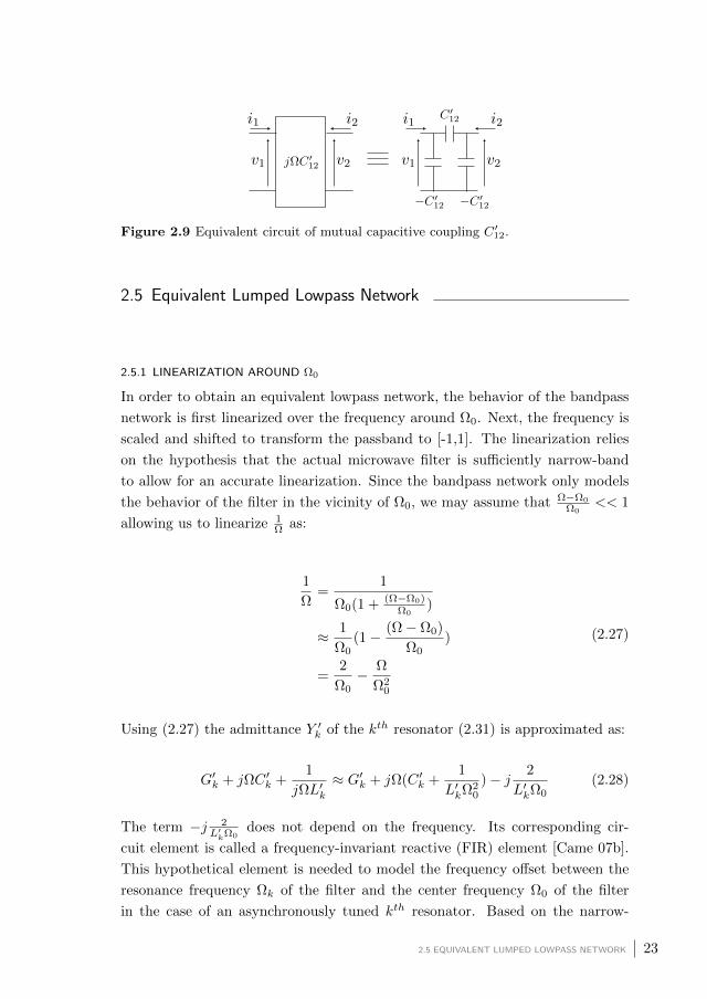
Figure 2.9 Equivalent circuit of mutual capacitive coupling C′12.

2.5 Equivalent Lumped Lowpass Network

2.5.1 LINEARIZATION AROUND Ω0

In order to obtain an equivalent lowpass network, the behavior of the bandpass

network is first linearized over the frequency around Ω0. Next, the frequency is

scaled and shifted to transform the passband to [-1,1]. The linearization relies

on the hypothesis that the actual microwave filter is sufficiently narrow-band

to allow for an accurate linearization. Since the bandpass network only models

the behavior of the filter in the vicinity of Ω0, we may assume that Ω−Ω0

Ω0<< 1

allowing us to linearize 1Ω as:

1

Ω=

1

Ω0(1 + (Ω−Ω0)Ω0

)

≈ 1

Ω0(1− (Ω− Ω0)

Ω0)

=2

Ω0− Ω

Ω20

(2.27)

Using (2.27) the admittance Y ′k of the kth resonator (2.31) is approximated as:

G′k + jΩC ′k +1

jΩL′k≈ G′k + jΩ(C ′k +

1

L′kΩ20

)− j 2

L′kΩ0(2.28)

The term −j 2L′kΩ0

does not depend on the frequency. Its corresponding cir-

cuit element is called a frequency-invariant reactive (FIR) element [Came 07b].

This hypothetical element is needed to model the frequency offset between the

resonance frequency Ωk of the filter and the center frequency Ω0 of the filter

in the case of an asynchronously tuned kth resonator. Based on the narrow-

2.5 EQUIVALENT LUMPED LOWPASS NETWORK 23

band hypothesis, the coupling between resonators is seen to become frequency

independent too:

jΩC ′kl ≈ jΩ0C′kl = jCkl (2.29)

Shifting and scaling the frequency Ω, transforms Ω to the lowpass frequency ω

such that the pass-band of the filter corresponds to the frequency range ω ∈[−1, 1]. To this end we define ω as follows:

ω =2

Ω2 − Ω1(Ω− Ω0) =

2

BW(Ω− Ω0) (2.30)

Using (2.30) we can now express the impedance under the linearized approxi-

mation (2.28) as a function of ω:

G′k + jωBW

2Ω0(C ′kΩ0 +

1

L′kΩ0) + j(C ′kΩ0 −

1

L′kΩ0) = Gk + jωCk + jBk (2.31)

where

Gk = G′k

Ck =FBW

2(C ′kΩ0 +

1

L′kΩ0)

Bk = (C ′kΩ0 −1

L′kΩ0)

(2.32)

Note that because Gk is frequency invariant, it remains unchanged under the

transformation. Also note that when 1√L′kC

′k

= Ω0, there is no frequency offset

with respect to Ω0 and thus Bk = 0. Applying Kirchoff’s Current Law in every

node of the network of Figure 2.10 yields the following result:


iS

0

0...

0

0

= ALP

US

U1

U2

...

UN

UL

(2.33)

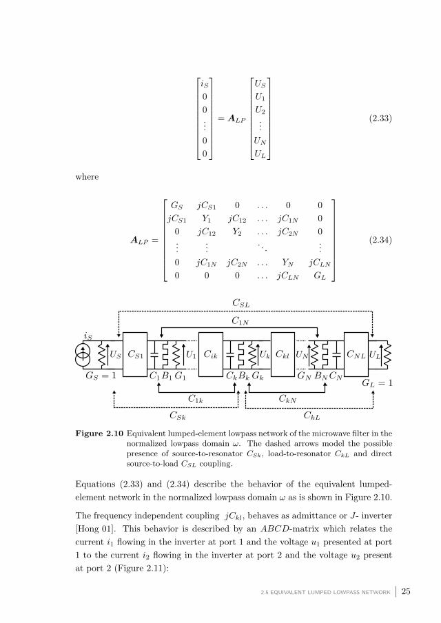
where

ALP =

GS jCS1 0 . . . 0 0

jCS1 Y1 jC12 . . . jC1N 0

0 jC12 Y2 . . . jC2N 0...

.... . .

...

0 jC1N jC2N . . . YN jCLN

0 0 0 . . . jCLN GL

(2.34)

Figure 2.10 Equivalent lumped-element lowpass network of the microwave filter in thenormalized lowpass domain ω. The dashed arrows model the possiblepresence of source-to-resonator CSk, load-to-resonator CkL and directsource-to-load CSL coupling.

Equations (2.33) and (2.34) describe the behavior of the equivalent lumped-

element network in the normalized lowpass domain ω as is shown in Figure 2.10.

The frequency independent coupling jCkl, behaves as admittance or J- inverter

[Hong 01]. This behavior is described by an ABCD-matrix which relates the

current i1 flowing in the inverter at port 1 and the voltage u1 presented at port

1 to the current i2 flowing in the inverter at port 2 and the voltage u2 present

at port 2 (Figure 2.11):


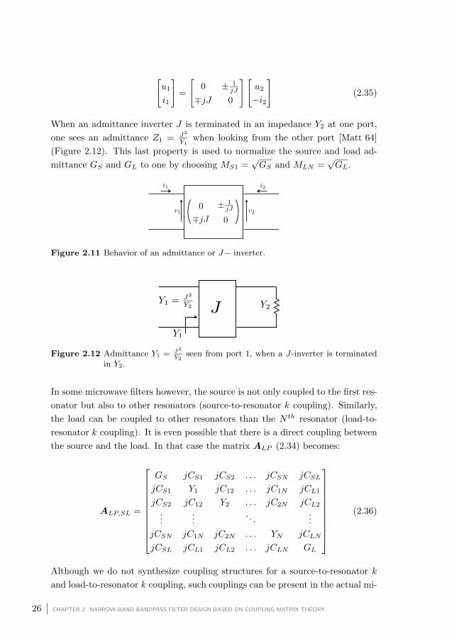
[u1

i1

]=

[0 ± 1

jJ

∓jJ 0

][u2

−i2

](2.35)

When an admittance inverter J is terminated in an impedance Y2 at one port,

one sees an admittance Z1 = J2

Y1when looking from the other port [Matt 64]

(Figure 2.12). This last property is used to normalize the source and load ad-

mittance GS and GL to one by choosing MS1 =√GS and MLN =

√GL.

Figure 2.11 Behavior of an admittance or J− inverter.

Figure 2.12 Admittance Y1 = J2

Y2seen from port 1, when a J-inverter is terminated

in Y2.

In some microwave filters however, the source is not only coupled to the first res-

onator but also to other resonators (source-to-resonator k coupling). Similarly,

the load can be coupled to other resonators than the N th resonator (load-to-

resonator k coupling). It is even possible that there is a direct coupling between

the source and the load. In that case the matrix ALP (2.34) becomes:

ALP,SL =

GS jCS1 jCS2 . . . jCSN jCSL

jCS1 Y1 jC12 . . . jC1N jCL1

jCS2 jC12 Y2 . . . jC2N jCL2

......

. . ....

jCSN jC1N jC2N . . . YN jCLN

jCSL jCL1 jCL2 . . . jCLN GL

(2.36)

Although we do not synthesize coupling structures for a source-to-resonator k

and load-to-resonator k coupling, such couplings can be present in the actual mi-


crowave filter. We already mention them here as they will prove to be important

in the remainder of the text.

2.5.2 DISCUSSION OF THE EQUIVALENT NETWORK BEHAVIOR

Due to the linearization of the term 1Ω (2.27) the order of the equivalent lowpass

network is halved (2.28) with respect to the bandpass filter. For the bandpass

lumped-element network (and thus for the actual microwave filter) the resonant

frequency of each resonator is double namely Ωk and −Ωk. This is no longer the

case for the equivalent lowpass network. The introduction of the FIR element

Bk accounts for the difference in resonant frequency of the LC-resonators in the

bandpass domain and the filter center frequency Ω0.

Section 2.6 introduces the coupling matrix representation of the lumped-element

circuit. This representation will be used here to implement the microwave filter.

Techniques exist to synthesize a lumped-element network from the polynomials

F ,P and E [Bele 68]. The synthesis techniques are not discussed in this work,

as we will synthesize the coupling matrix directly from F ,P and E instead and

will hereby avoid the synthesis of the network all together.

2.5.3 LINK TO THE CLASSICAL BANDPASS-TO-LOWPASS TRANSFORMATION

In classical network synthesis a different bandpass-to-lowpass frequency trans-

formation is often used to go from the bandpass to the lowpass domain:

ω =1

FBW(

Ω

Ω0− Ω0

Ω) (2.37)

The advantage of the classical bandpass-to-lowpass transformation is that it

transforms all lowpass circuit elements to bandpass resonators resonating at

Ω0, which is the case for all the symmetrical responses. In microwave filters

having asymmetrical responses, the resonators are not synchronously tuned. The

transformation given by (2.37) also yields the equivalent lumped lowpass network

presented in Section 2.5 if FIR elements are included in the bandpass domain

to model the offset between individual resonant frequency of resonator and the

center frequency of the filter [Came 07b]. Note that the classical transformation

transforms the positive (around Ω0) and negative (around −Ω0) bandpass image

to the lowpass domain. The linearization as is used here only takes the positive

bandpass behavior around Ω0 into account. Both transformations result in a

lowpass prototype that has half the order of the original bandpass filter.


2.6 Coupling Matrix Representation

This section introduces the coupling matrix representation of coupled-resonator

filters. One of the benefits is that matrix operations such as an inversion or a

similarity transformation can be applied to the coupling matrix directly resorting

to network transformations. These operations simplify both the analysis and the

synthesis of the microwave filter.

Moreover the coupling matrix elements can easily be linked to the elements in

the microwave filter, which simplifies the diagnosis as well as the tuning.

We discuss next how the coupling matrix can be derived from the lowpass

lumped-element circuit. This coupling matrix used here is referred to as the

N + 2 coupling matrix, as it also contains source-to-resonator k coupling, load-

to-resonator k coupling and source-to-load coupling [Came 03]. At the end of

this section we introduce the admittance (Y -) parameters and use them to dis-

cuss the relation between the coupling matrix and the state-space representation

based on the Y -parameters. In Section 2.7 we use this relation to synthesize the

coupling matrix from F ,P and E.

2.6.1 THE N + 2 COUPLING MATRIX

Dividing row k ∈ 2, . . . , N by√Ck−1 and dividing column l ∈ 2, . . . , N by√

Cl−1 normalizes the set of equations given in (2.33) and (2.34). The normalized

matrix ALP becomes:


A =

1 j CS1√C1

0 . . . 0 0

j LS1√C1

jω + jB1

C1+ G1

C1j C12√

C1C2. . . C1N√

C1CN0

0 j C12√C1C2

jω + jB2

C2+ G2

C2. . . j C2N√

C2CN0

......

. . ....

0 j C1N√C1CN

j C2N√C2CN

. . . jω + jBNCN + GNCN

j CLN√CN

0 0 0 . . . j CLN√CN

1

=

1 jMS1 0 . . . 0 0

jMS1 jω + jM11 + G1

C1jM12 . . . jM1N 0

0 jM12 jω + jM22 + G2

C2. . . jM2N 0

......

. . ....

0 jM1N jM2N . . . jω + jMNN + GNCN

jMLN

0 0 0 . . . jMLN 1

= M +G+ jωIN+2

(2.38)

Herein, the matrix M is called the N + 2 coupling matrix, which is obtained as:

M =

1 jMS1 0 . . . 0 0

jMS1 jM11 jM12 . . . jM1N 0

0 jM12 jM22 . . . jM2N 0...

.... . .

...

0 jM1N jM2N . . . jMNN jMLN

0 0 0 . . . jMLN 1

(2.39)

The inner part of M containing rows k ∈ 2, . . . , N + 1 and columns l ∈2, . . . , N + 1) describes the inter-resonator coupling and is defined as the N ×N coupling matrix. The diagonal elements Mkk define the self-couplings. A

coupling Mk(k+1) is called a sequential coupling and a coupling Mlk (k 6= l +

1,resonator l and k are not adjacent) is called a cross-coupling.

The matrix G contained in (2.38) is a diagonal matrix of size (N + 2)× (N + 2)

where the diagonal elements are GkCk

and the first and last elements of the diagonal

are 0. WritingGk and Ck as a function of the bandpass equivalent elements yields

(2.32)):

2.6 COUPLING MATRIX REPRESENTATION 29

GkCk

=1

Qk

1

FBW(2.40)

These elements can be interpreted as the inverse of the quality factor Qk of

the kth LC resonator of the bandpass equivalent if the non-diagonal coupling

elements are purely imaginary [Came 07b]. The matrix IN+2 is an identity

matrix of size (N +2)× (N +2) where the first and last elements of the diagonal

are 0. Figure 2.13 shows the equivalent network that is represented by the matrix

A.

To denormalize the bandwidth of the coupling matrix, it suffices to multiply

the inter-resonator couplings Mkl and frequency offsets Mkk by FBW and the

source-to-resonator and load-to-resonator coupling by√FBW (2.32).

Figure 2.13 Equivalent lumped-element lowpass network of the microwave filter thatis represented by the matrix A

2.6.2 S-PARAMETERS AS A FUNCTION OF A

It is possible to express the S-parameters as a function of A−1. Multiplying

both sides of (2.33) by A−1 yields:

A−1

iS

0

0...

0

0

=

US

U1

U2

...

UN

UL

(2.41)


Which allows to write:

US = [A−1]1,1iS

UL = [A−1]N+2,1iS(2.42)

where [A]k,l denotes element (k, l) of the matrix A. Since GS = GL = 1, we

also have that (Figure 2.13):

i1 = iS − USi2 = −v2 = −UL

(2.43)

Using the definitions for the S-parameters for a normalized impedance (ZS =

ZL = 1) ((2.4)) we write:

S11 =v1 − i1v1 + i1

=US − i1iS

=US − (iS − US)

iS

=iS(2[A−1]1,1 − 1)

iS

= 2[A−1]1,1 − 1

(2.44)

S21 =v2 − i2v1 + i1

=UL − i2iS

=2ULiS

=iS(2[A−1]N+2,1)

iS

= 2[A−1]N+2,1

(2.45)

To calculate S12 and S22 as a function of the elements of A−1, an ideal current

source providing current iL in parallel with a normalized conductance GL = 1

must be presented at port 2 and port 1 must be terminated in a normalized

conductance GS = 1. This yields:


i1 = −v1 = −USi2 = iL − UL

(2.46)

S22 =v2 − i2v2 + i2

=UL − i2iL

=iL(2[A−1]N+2,N+2 − 1)

iL

= 2[A−1]N+2,N+2 − 1

(2.47)

S12 =v1 − i1v2 + i2

=US − i2iL

=iL(2[A−1]1,N+2)

iL

= 2[A−1]1,N+2

(2.48)

Expressions (2.44), (2.45), (2.47) and (2.48) will be used to calculate the sen-

sitivity of the S-parameters with respect to the the elements of the coupling

matrix M (2.39).

2.6.3 LINK TO THE STATE-SPACE REPRESENTATION

The Admittance Matrix Y

When the filter is represented by a linear time-invariant two-port network (Fig-

ure 2.1), the admittance (Y -) parameters relate the input port voltage v1 and

output port voltage v2 to the input port current i1 and output port current i2

[Poza 98]:

Y11 =i1v1

∣∣∣∣v2=0

Y12 =i1v2

∣∣∣∣v1=0

(2.49)

Y21 =i2v1

∣∣∣∣v2=0

Y22 =i2v2

∣∣∣∣v1=0

(2.50)

The Y -parameters can also be grouped in the admittance matrix Y :


[i1

i2

]=

[Y11 Y12

Y21 Y22

][v1

v2

]= Y

[v1

v2

](2.51)

Note that the Y -matrix models the behavior of the filter as a function of

frequency. An equivalent representation of the dynamics contained in the Y -

parameters is contained in the state-space representation.

State-space representation of the equivalent lowpass network

The state-space representation [Kail 80] of the Y -parameter matrix is:

x(t) = AY x(t) +BY

[v1(t)

v2(t)

]

[i1(t)

i2(t)

]= CY x(t) +DY

[v1(t)

v2(t)

] (2.52)

with

• x : a vector of size N × 1 containing the states of the system, also called

the state-vector

• x : the time derivative of the state-vector of size N × 1

• AY : the system matrix of size N ×N

• BY : the input matrix of size N × 2

• CY : the output matrix of size 2×N

• DY : the direct transmission matrix of size 2× 2

We now determine the state-space representation of the system starting from the

Y -parameters of the low-pass equivalent network. We consider the general case

where every resonator is coupled to the source and the load and there is a direct

source to load coupling. We consider the N rows k ∈ 2, . . . , N + 1 of ALP,SL

((2.36)) and write (2.33) in the time-domain. Next, we group the derivative

of [U1, . . . , UN ]t on the left hand side (LHS) and we split up the contributions

of [U1, . . . , UN ]t and [US , UL]t on the right hand side (RHS) of the resulting

expression as follows:


dU1(t)dt

dU2(t)dt...

dUN (t)dt

=

−G1+jB1

C1− jC12

C1. . . − jC1N

C1

− jC12

C2−G2+jB2

C2. . . − jC2N

C2

......

. . ....

− jC1N

CN− jC2N

C2. . . −GN+jBN

CN

U1(t)

U2(t)...

UN (t)

+

−j CS1

C1−j CL1

C1

−j CS2

C2−j CL2

C2

......

−j CSNCN−j CLNCN

[US

UL

](2.53)

The first and last row of ALP,SL ((2.36)) allow to determine i1 and i2. Since

i1 = iS −GSUS and i2 = iL −GLUL, we write:

[i1

i2

]=

[jCS1 jCS2 . . . jCSN

jCL1 jCL2 . . . jCLN

]

U1(t)

U2(t)...

UN (t)

+

[0 jCSL

jCSL 0

][US

UL

](2.54)

Equations (2.53) and (2.54) are a state-space representation of the admittance

parameters of the lowpass equivalent network. The states in this case are the

voltages U = [U1, . . . , UN ]t. This state-vector U however can be transformed to

another state-vector x = PU , where P is an invertible matrix of size N × N .

Applying the transformation P to a state-space representation yields:

xP = Px

APY = PAY P−1

BPY = PBY

CPY = CY P−1

(2.55)

Assume that we choose P such that the state-vector U is transformed to obtain a

system matrix that is symmetric and an input matrix that becomes the transpose

of the output matrix. To this end, we choose P as:


P =

j√C1 0 . . . 0

0 j√C2 . . . 0

.... . .

...

0 . . . 0 j√CN

(2.56)

Applying the transformation P to (2.53) and (2.54) yields:

x =

−G1+jB1

C1− jC12√

C1C2. . . − jC1N√

C1CN

− jC12√C1C2

−G2+jB2

C2. . . − jC2N√

C2CN...

.... . .

...

− jC1N√C1CN

− jC2N√C2CN

. . . −GN+jBNCN

x+

CS1√C1

CL1√C1

CS2√C2

CL2√C2

......

CSN√CN

CLN√CN

[v1

v2

]

[i1

i2

]=

[CS1√C1

CS2√C2

. . . CSN√CN

CL1√C1

CL2√C2

. . . CLN√CN

]x+

[0 jCSL

jCSL 0

][v1

v2

]

(2.57)

Using the notation introduced in Section 2.6.1 we write (2.57) as:

x =

−jM11 − G1

C1−jM12 . . . −jM1N

−jM12 −jM22 − G2

C2. . . −jM2N

......

. . ....

−jM1N −jM2N . . . −jMNN − GNCN

x

+

MS1 ML1

MS2 ML2

......

MSN MLN

[v1

v2

]

[i1

i2

]=

[MS1 MS2 . . . MSN

ML1 ML2 . . . MLN

]x+

[0 jCSL

jCSL 0

][v1

v2

]

(2.58)

Where x = PU . In the case of a lossless filter, where only the first resonator is

coupled to the source and the last resonator is coupled to the load the state-space

representation of (2.58) becomes:


x =

−jM11 −jM12 . . . −jM1N

−jM12 −jM22 . . . −jM2N

......

. . ....

−jM1N −jM2N . . . −jMNN

x+

MS1 0

0 0...

...

0 MLN

[v1

v2

]

[i1

i2

]=

[MS1 0 . . . 0

0 0 . . . MLN

]x

(2.59)

(2.59) shows that if the system matrix is symmetrical and the input matrix is

the transpose of the output matrix, the system matrix APY is equal to the

N ×N coupling matrix with a negative sign. Moreover the input BPY and out-

put CPY matrix contain the source-to-resonator couplings and load-to-resonator

couplings. The direct transmission matrix DY only exist in the case of a direct

source-to-load coupling. Note that applying a similarity transformation to the

coupling matrix preserves the frequency response while it changes the coupling

matrix. This means that the coupling matrix is not unique representation and

thus several equivalent coupling matrices exist that realize the same filter.

Transforming (2.58) back to the frequency domain and eliminating the state-

vector allows to write the Y -parameters as a function of the state-space matrices:

Y (s) = CY (sIN −AY )−1BY +DY (2.60)

Herein, (AY ,BY ,CY ,DY ) is also called a realization of Y .

2.7 Synthesis of the Coupling Matrix

This section explains how to perform the synthesis of a coupling matrix starting

from the polynomials F ,P and E found in Section 2.3. First we transform the

S-matrix to the Y -matrix using the Cayley transformation. Next we construct

a minimal realization of the Y -matrix using Gilbert’s method [Gilb 63]. Finally,

we transform the obtained realization to a canonical form. In this case we

choose the arrow form [Seyf 98]. The obtained system matrix corresponds to

the canonical arrow form coupling matrix up to a sign change (2.59).


2.7.1 CAYLEY TRANSFORMATION AND PROPERTIES OF Y

The scattering matrix S is transformed to the admittance matrix Y using the

Cayley transformation:

Y = (I2 − S)(I2 + S)−1 (2.61)

Applying the transformation to (2.16) yields Y as a function of F ,P and E:

Y =

[E − F + (−1)N+1(E∗ − F ∗) −2P

−2P E + F + (−1)N+1(E∗ + F ∗)

]

E + F + (−1)N (F ∗ + E∗)

=1

q

[n11 n12

n12 n22

] (2.62)

Note that since F and E are monic, the numerators of Y11 and Y22 are of degree

N − 1. The admittance matrix has a common denominator:

q = E + F + (−1)N (F ∗ + E∗) (2.63)

Since the filter is passive and loss-less the corresponding Y -matrix verifies the

conditions [Ande 73]:

Y (jω) + Y H(jω) = 0 (2.64)

Y (s) + Y H(s) ≥ 0 , for Re(s) = σ ≥ 0 (2.65)

Note that these relations express the same properties as (2.14) and (2.15). Due

to the analytic continuation of Y (2.64) implies:

Y (s) = −Y ∗(s) (2.66)

This means that the poles of Y must be symmetrical with respect to the imag-

inary axis. If si is a pole of Y , by (2.66) we have that:

2.7 SYNTHESIS OF THE COUPLING MATRIX 37

q(si) = 0⇒ q∗(si) = 0 (2.67)

Using the definition of the para-conjugation we can write:

q∗(si) = q(−si) = 0 (2.68)

which yields:

q(−si) = 0⇒ q(−si) = 0 (2.69)

(2.69) shows that if si is a pole of Y , −si is also a pole of Y and therefore the

poles must lie symmetrically with respect to the imaginary axis.

Due to (2.65) the real part of Y is a semi-positive matrix of s when the real part

of s is equal or greater than zero. This implies that the real part of the diagonal

elements of Y , Y11 and Y22 is non-negative when evaluated for s in the right half

plane. We will use this property to show that the poles are purely imaginary,

simple and that their residues are non-negative.

In the vicinity of a pole si of multiplicity n of Y11(s) (the rationale is similar for

Y22), we have that:

Y11(s)R

(s− si)n=

rejφ

(s− si)n, for s→ si (2.70)

where R ∈ C. Assume that Y11 has a pole si in the right half plane. On a circle

with a center si and a radius ρ (s = si + ρejθ), we can write:

Y11(s) ≈ rejφ

ρejnθ=r

ρej(φ−nθ) (2.71)

The real part of (2.71) is:

Re(Y11(s)) =r

ρcos(φ− nθ) (2.72)

If we run over a circle around a pole in the right half plane (θ : 0 → 2π), the

sign of Re(Y11(s)) changes n times. This is in contradiction with the fact that

Re(Y11(s)) ≥ 0 for σ ≥ 0, thus Y has no poles in the right half plane. In


combination with the fact that the poles must lie symmetrically with respect to

the imaginary axis, this yields that the poles must lie on the imaginary axis.

If we now run over the part of a circle around an imaginary pole jωi that lies in

the right half plane (θ : −π2 → π2 ), the sign of Re(Y11(s)) does not change if and

only if n = 1 and φ = 0. This shows that the multiplicity of jωi is 1. Moreover

since R = rejφ = r is the residue of the pole, this shows that the residue is real

and positive.

Since the poles are simple and purely imaginary, Y admits the following partial

expansion :

Y =

N∑

k=1

R(k)

s− jωk=

N∑

k=1

[r

(k)11 r

(k)12

r(k)21 r

(k)22

]

s− jωk(2.73)

Substituting (2.73) in (2.66) yields:

−N∑

k=1

R(k)

s− jωk=

N∑

k=1

RH(k)

−s+ jωk(2.74)

Thus we have that R(k) = RH(k). Since R(k) is symmetrical, we also have that

R(k) = Rt(k) and therefore R(k) is a real symmetric matrix.

Substituting (2.73) in (2.65) yields:

Y + Y H =

N∑

k=1

R(k)(1

s− jωk+

1

s+ jωk) =

N∑

k=1

R(k)2 Re(s)

|s− jωk|2(2.75)

Since Y + Y H is semi-positive definite matrix for σ ≥ 0, we have ∀x ∈ C2:

xH(Y + Y H)x =

N∑

k=1

xHR(k)x2σ

|s− jωk|2≥ 0 (2.76)

(2.76) is only true if xHR(k)x ≥ 0 and therefore R(k) is also a semi-positive

definite matrix.

Writing Y21 = Y12 in its pole-residue form yields:


Y21(s) =

N∑

k=1

r(k)21

s− jωk=

N∑k=1

r(k)21

∏Ni=1,i6=k(s− jωi)

∏Ni=k s− jωk

(2.77)

(2.77) shows that the coefficient corresponding to sN−1 of the numerator isN∑k=1

r(k)21 . Since nfz < N − 1, this coefficient must be zero:

N∑

k=1

r(k)21 = 0 (2.78)

It is shown in classical realization theory that if a transfer function Y has simple

poles and thus admits an expansion as (2.73), the residues verify ([Kail 80],p.349):

N∑

k=1

rank(R(k)) = N (2.79)

This is equivalent to:

∀k, rank(R(k)) = 1⇒ det(R(k)) = 0 (2.80)

Summary of the Obtained Properties of Y

The admittance matrix Y (s) of a filter can be obtained by transforming S(s)

using the Cayley transform ((2.61)). In the case of a passive and loss-less filter

with maximally N − 2 finite transmission zeros, Y (s) admits a partial fraction

expansion of the form (2.73), where the residues:

R(k) =

[r

(k)11 r

(k)12

r(k)12 r

(k)22

](2.81)

verify the following properties:

r(k)11 , r

(k)22 , r

(k)12 ∈ R

r(k)11 ≥ 0 and r

(k)22 ≥ 0

r(k)11 r

(k)22 − (r

(k)12 )2 = 0

N∑k=1

r(k)12 = 0

(2.82)


2.7.2 MINIMAL REALIZATION OF Y

If Y is a proper rational matrix, then it admits a realization. In this section we

construct a realization of Y (s), (AY ,BY ,CY ,DY ) that verifies AY = AtY and

BY = CtY . Moreover the size of AY is equal to N ×N .

The degree of a realization (AY ,BY ,CY ,DY ) is defined as the size of the matrix

AY . We define the McMillan degree as the minimum of the degree of all possible

realizations of Y . If (AY ,BY ,CY ,DY ) is a realization of Y it is minimal if and

only if its degree is equal to the McMillan degree of Y [Kail 80].

If (A(1),B(1),C(1),D(1)) and (A(2),B(2),C(2),D(2)) are two minimal realiza-

tions of the same proper rational matrix, there exists a unique invertible matrix

P such that:

A(2) = P−1A(1)P

B(2) = P−1B(1)

C(2) = C(1)P

D(2) = D(1)

(2.83)

This means that once we find a minimal realization we can transform it to any

other minimal realization. In the case where a rational matrix has simple poles,

Gilbert’s realization is a minimal realization for which the system matrix is

diagonal. We now apply Gilbert’s method [Gilb 63] to the admittance matrix

Y found in (2.62).

Section 2.7.1 shows that Y admits the following expansion:

Y =

N∑

k=1

R(k)

s− jωk=

N∑

k=1

[r

(k)11 r

(k)12

r(k)21 r

(k)22

]

s− jωk(2.84)

where

r(k)11 r

(k)22 − (r

(k)12 )2 = 0 (2.85)

This means that Rk can be written as


Rk = CkBk =

r(k)12√r(k)22√r

(k)22

[r(k)12√r(k)22

√r

(k)22

](2.86)

Remark that Ck = Btk. If we now write Cd and Bd as the concatenation of Ck

and Bk respectively, we can rewrite Y ((2.84)) as:

Y =

r(1)12√r(1)22

r(2)12√r(2)22

. . .r(N)12√r(N)22√

r(1)22

√r

(2)22 . . .

√r

(N)22

jω1 0 . . . 0

0 jω2 . . . 0...

. . ....

0 . . . 0 jωN

r(1)12√r(1)22

√r

(1)22

r(2)12√r(2)22

√r

(2)22

......

r(N)12√r(N)22

√r

(N)22

= Cd(sIN −Ad)−1Bd

(2.87)

The corresponding N + 2 coupling matrix is (2.59):

Md =

1 jr(1)12√r(1)22

jr(2)12√r(2)22

. . . jr(N)12√r(N)22

0

jr(1)12√r(1)22

−jω1 0 . . . 0 j

√r

(1)22

jr(2)12√r(2)22

0 −jω2 . . . 0 j

√r

(2)22

......

. . ....

jr(N)12√r(N)22

0 0 . . . −jωN j

√r

(N)22

0 j

√r

(1)22 j

√r

(2)22 . . . j

√r

(N)22 1

(2.88)

The coupling matrix Md is better known as the transversal N + 2 coupling

matrix and (2.88) is the same as the relation found in [Came 03]. Remark that

Md is not unique. If the ordering of the poles changes, Md changes as well

without affecting Y .

Finally note that due to (2.78) and (2.85), we have that:


CdBd = BtdBd =

N∑k=1

r(k)11 0

0N∑k=1

r(k)22

(2.89)

which also shows that the columns of Bd are orthogonal and their norms are

equal toN∑k=1

r(k)11 and

N∑k=1

r(k)22 respectively.

2.7.3 ARROW FORM OF THE N ×N COUPLING MATRIX

It can be shown that if a matrixAr is a real symmetric matrix of sizeN×N , there

exists an orthogonal transformation Pf (Pf = P tf ) such that P−1

f ArPf = Af

has the arrow form [Seyf 98]:

Af =

∗ ∗ (0) ∗

∗ . . .. . .

...

(0). . .

. . . ∗∗ . . . ∗ ∗

(2.90)

Where all the entries of Af must be zero except for those on the diagonal,

the first upper-diagonal, the first lower-diagonal, and those in the last row and

column. If all of the elements lower-diagonal are non zero the transformation

Pf is unique up to sign changes, meaning that Af is unique up to sign changes

and thus is a canonical form [Seyf 07]. The first and the last column of the

transformation matrix Pf are chosen to be the normalized first and last column

of Bd. The vectors are normalized by dividing each element by the 2-norm of

the vector. Applying transformation Pf to the Gilbert realization (Ad,Bd,Cd)

yields a canonical realization (Af ,Bf ,Cf ) where

Bf = Ctf =

N∑k=1

r(k)11 0

0 0...

...

0N∑k=1

r(k)22

(2.91)

Remark that other canonical forms exist such as the folded form [Came 99].


2.8 Reconfiguration of the Coupling Matrix

Section 2.7 explains how to synthesize a coupling matrix in the arrow form

starting from F ,P and E. Although this form is canonical it is not always

possible to implement it physically, due to its associated coupling topology. The

coupling topology of the filter describes the way that the resonators are coupled

to each other. To make this structure more easy to interpret, we represent

the coupling topology by a coupling graph (Figure 2.14) in this work. In the

case of the arrow form all adjacent resonators are coupled to each other and

every resonator is coupled to the last resonator. In a planar technology such

as a microstrip technology it is not always practically possible to obtain such

an implementation. Therefore the coupling matrix is usually transformed by

similarity transformation to obtain a more practical coupling topology. There

are however limitations: it is impossible to implement an arbitrary filter function

in an arbitrary coupling topology. In this section we list up the conditions that

are necessary to ensure that a certain filter function is compatible with a specific

coupling topology.

Figure 2.14 Coupling graph of the arrow form coupling topology. A black node rep-resents a resonator, the gray nodes represent the source and the loadand a full line represents a coupling. For the arrow form all sequentialresonators are coupled and each resonator is coupled to the last resonator.When a self-coupling is non zero the resonator is presented by a full blacknode, otherwise by a white node.

2.8.1 SHORTEST PATH RULE

For a given topology, define l to be the shortest path length (= number of

connections) between the source and the load in a coupling graph (Figure 2.14).

Physically, l is the number of couplings present between the load and the source.

Theorem 1 (Shortest Path Rule). The maximum number of finite transmission

zeros accommodated by the coupling topology containing N resonators and having

a shortest path length l between the source and the load is N + 1− l.


The proof of the shortest path rule is given in [Amar 99].

The shortest path rule allows to evaluate the number of finite transmission ze-

ros accommodated by a specific coupling topology. When a coupling topology

contains a direct source-to-load coupling MSL, the smallest number of connec-

tions between the source and the load is 1. Thus the shortest path length is 1

(l = 1). In that case the number of finite transmission zeros accommodated by

the coupling topology is N .

In this work we do not synthesize coupling topologies with a direct source-to-

load coupling. In the case of no direct source-to-load coupling, the shortest

possible path between the source and the load in a coupling topology consists

of 3 connections. This occurs when there is a coupling between the input and

the output resonator. In that case the shortest path consists of one source-

to-resonator coupling MS1, one inter-resonator coupling M1N and one load-

to-resonator coupling MNL, which makes that the shortest path length is 3.

Therefore the maximal number of finite transmission zeros accommodated by

the filters in this work is N − 2.

2.8.2 COMPATIBILITY BETWEEN THE FILTER RESPONSE AND THE COUPLING TOPOL-

OGY

Two filter responses are said to be part of the same class of filter responses

if they have the same order N , the same number of finite transmission zeros

nfz and their frequency responses are both symmetrical or both asymmetrical

with respect to the center frequency [Seyf 07]. N , nfz and the fact whether the

response is symmetrical or asymmetrical sets the number of degrees of freedom

that can be used in the filter response. We call this number the dimension

of the class. For a filter response it is possible to determine the number of

real independent parameters that define P and F . This number is exactly the

number of degrees of freedom that can be used in the filter response. We now

determine the dimensions of the general class of symmetric and asymmetric filter

responses having an order N and nfz finite transmission zeros.

For an asymmetric filter response of order N having nfz finite transmission zeros

we can choose N complex reflection zeros (yielding N complex coefficients of F

and thus 2N independent parameters). Due to its para-conjugated nature the

coefficients of P alternate between purely real and purely imaginary numbers.

Since there are nfz finite transmission zeros, P has nfz + 1 independent real

coefficients only. Therefore, the dimension of the general class of asymmetric

filter characteristics of order N having nfz finite transmission zeros is 2N +

2.8 RECONFIGURATION OF THE COUPLING MATRIX 45

nfz + 1.

For symmetric filter response characteristics, the coefficients of F must be real.

Therefore, F has N independent real coefficients. Since the transmission zeros

are also symmetric with respect to the center frequency, P is an even polynomial

and thus nfz is even as well resulting innfz

2 degrees of freedom. The dimension of

the class of symmetric filter responses of order N having nfz finite transmission

zeros therefore is N +nfz

2 + 1.

In order for a coupling topology to accommodate for a class of filter responses,

the number of independent coupling parameters of the coupling topology must

at least be equal to the dimension of the filter responses. If these numbers are

equal, the realization problem has a finite number of solutions this includes the

possibility that no solution exists [Seyf 07].

Compatibility between Class of Responses and the Arrow Form

Topology

The arrow form topology (Figure 2.14) has N self-couplings Mkk, N −1 sequen-

tial couplings Mk(k+1) (k 6= N), N − 2 cross-couplings between each resonator

and resonator N and two input and output couplings. This results in 3N − 1

coupling parameters in total. Since the first resonator is coupled to the last

resonator and there is no direct source-to-load coupling, the shortest path rule

says that there can be N − 2 finite transmission zeros. The dimension of the

class of asymmetric filter responses of order N , having N − 2 transmission zeros

is also 2N + N − 2 + 1 = 3N − 1. If the shortest path enlarges by eliminating

couplings to resonator N , the number of admissible finite transmission zeros

decreases. If we eliminate all couplings MkN , the shortest path becomes N − 1

and thus we have no more finite transmission zeros. This corresponds to the

classical Chebyshev response, where only sequential couplings are present.

It is shown [Bell 82] that coupling topologies where Mkl = 0 if k + l is even,

are symmetric. In the case of the arrow form, this means that all self-couplings

Mkk and every second cross-coupling to the last resonator become zero. If N

is even this means that each element MkN is zero if k is even, yielding N−22

non-zero cross-coupling. The number of non-zero elements in the arrow form is

N − 1 + N−22 + 2, which corresponds to the dimension of the class of (N,N − 2)

symmetric filter responses. In the case where N is odd, each element MkN is zero

if k is odd. This means that the shortest path is enlarged by one, yielding only

N − 3 transmission zeros (which is consistent with the fact the zeros are located

symmetrically with respect to the center frequency). The number of non-zero


elements in this case is N − 1 + N−32 + 2, which corresponds to the dimension of

the class of (N,N − 3) symmetric filter responses (where N is odd).

Finally note that a coupling topology is said to be canonical for a class of fil-

ter responses if it is unique and has exactly the same number of independent

parameters as the dimension of the class [Seyf 07].

2.8.3 RECONFIGURATION TO A GENERAL COUPLING TOPOLOGY

In this work we focus on the class of topologies made of cascaded triplets and

quadruplets. For this coupling topologies, the compatibility condition given in

Section 2.8.2 is sufficient to guarantee the existence of a solution of the re-

alization problem. In the case of cascaded triplet and quadruplet topologies

multiple solutions exist. Reconfiguring a coupling matrix to a desired coupling

topology is also called coupling matrix reduction, since the process eliminates

certain couplings. Various approaches, based on optimization have been pro-

posed to solve the reduction problem [Atia 98; Amar 00b]. The main drawback

of these methods is that they do not necessarily yield all the possible solutions.

Therefore a procedure that is based on Groebner basis and homotopy tech-

niques has been developed. This method solves the underlying non-linear set

of equations to yield all of the possible solutions for all of the relevant topolo-

gies [Came 07a; Came 05]. This technique has been implemented in the Matlab

toolbox DEDALE-HF [Seyf 00], which we use to reconfigure the coupling matrix

here.


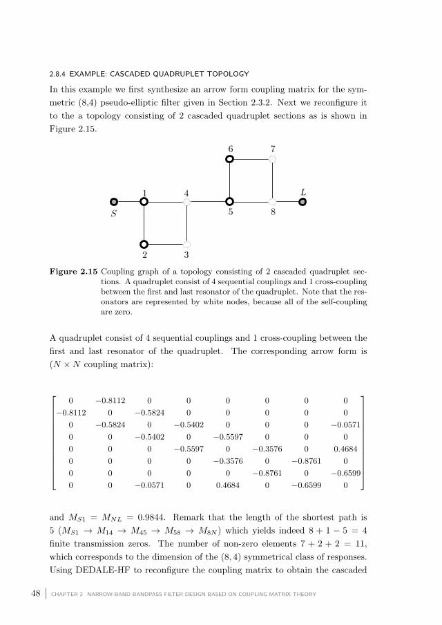
2.8.4 EXAMPLE: CASCADED QUADRUPLET TOPOLOGY

In this example we first synthesize an arrow form coupling matrix for the sym-

metric (8,4) pseudo-elliptic filter given in Section 2.3.2. Next we reconfigure it

to the a topology consisting of 2 cascaded quadruplet sections as is shown in

Figure 2.15.

Figure 2.15 Coupling graph of a topology consisting of 2 cascaded quadruplet sec-tions. A quadruplet consist of 4 sequential couplings and 1 cross-couplingbetween the first and last resonator of the quadruplet. Note that the res-onators are represented by white nodes, because all of the self-couplingare zero.

A quadruplet consist of 4 sequential couplings and 1 cross-coupling between the

first and last resonator of the quadruplet. The corresponding arrow form is

(N ×N coupling matrix):

0 −0.8112 0 0 0 0 0 0

−0.8112 0 −0.5824 0 0 0 0 0

0 −0.5824 0 −0.5402 0 0 0 −0.0571

0 0 −0.5402 0 −0.5597 0 0 0

0 0 0 −0.5597 0 −0.3576 0 0.4684

0 0 0 0 −0.3576 0 −0.8761 0

0 0 0 0 0 −0.8761 0 −0.6599

0 0 −0.0571 0 0.4684 0 −0.6599 0

and MS1 = MNL = 0.9844. Remark that the length of the shortest path is

5 (MS1 → M14 → M45 → M58 → M8N ) which yields indeed 8 + 1 − 5 = 4

finite transmission zeros. The number of non-zero elements 7 + 2 + 2 = 11,

which corresponds to the dimension of the (8, 4) symmetrical class of responses.

Using DEDALE-HF to reconfigure the coupling matrix to obtain the cascaded


quadruplet topology yields 2 possible solutions:

0 0.7425 0 −0.3269 0 0 0 0

0.7425 0 0.7917 0 0 0 0 0

0 0.7917 0 0.4522 0 0 0 0

−0.3269 0 0.4522 0 0.5265 0 0 0

0 0 0 0.5265 0 0.5116 0 −0.1567

0 0 0 0 0.5116 0 0.6852 0

0 0 0 0 0 0.6852 0 0.7960

0 0 0 0 −0.1567 0 0.7960 0

and

0 0.7960 0 −0.1567 0 0 0 0

0.7960 0 0.6852 0 0 0 0 0

0 0.6852 0 0.5116 0 0 0 0

−0.1567 0 0.5116 0 0.5265 0 0 0

0 0 0 0.5265 0 0.4522 0 −0.3269

0 0 0 0 0.4522 0 0.7917 0

0 0 0 0 0 0.7917 0 0.7425

0 0 0 0 −0.3269 0 0.7425 0

The fact that there are 2 solutions can be interpreted as follows; each quadru-

plet creates a pair of transmission zeros that is symmetric with respect to the

center frequency. There are 2 ways of doing this. In the first solution the first

quadruplet creates the (-1.2,1.2) pair and the second one the (-1.5,1.5) pair. For

the other solution it is the other way around, the pairs are inverted.


3Physical Implementation of the Coupling Matrix in Microstrip Technol-

ogy

This chapter introduces a method to obtain initial values for the physical param-

eters of the actual microwave filter that is to be realized. The idea is to select the

physical dimensions of the filter such that coupling matrix of the actual filter is

close to the ideal or target coupling matrix. The dimensioning method described

in this chapter first divides the filter into building blocks. It dimensions these

blocks separately and finally merges them to obtain the complete filter. This

method is applicable to a general physical realization, but in this work we focus

on microstrip filters.

This chapter first introduces the microstrip transmission line structure. Sec-

tion 3.2 summarizes some important characteristics of the microstrip line. Sec-

tion 3.3 introduces the half-wavelength or λ2 resonators, that are used to realize

the filters. Full wave electromagnetic (EM) field solvers are intensively used to

investigate the behavior of coupled-resonator structures and to design the filters.

Section 3.4 discusses the use of the EM-solvers and their simulation settings.

Section 3.5 explains the dimensioning method for microstrip resonators in de-

tail. Finally Section 3.6 applies the method to design a fourth order quadruplet

square-open-loop resonator (SOLR) filter.

3.1 Introduction

In this chapter we explain how to obtain initial values for the physical parameters

of the actual microwave filter obtained from the design before. To physically im-

plement the coupling matrix obtained in Chapter 2, the layout of the microwave

resonators is selected to correspond to the coupling topology. Moreover the res-

onators are dimensioned to have the desired frequency offset with respect to the

center frequency of the prototype filter and the input/output and inter-resonator

51

distance is selected to approximate the ideal coupling as closely as possible. The

dimensioning method described in this chapter divides the filter into building

blocks consisting of individual or pairs of resonators. Next, it dimensions these

blocks separately and finally merges them to obtain the complete filter. There-

fore it is sometimes referred to as the ’divide and conquer strategy’ [Came 07b].

The building blocks used to represent coupled resonator filters are typically the

input/output resonator and sections consisting of 2 coupled resonators. The

dimensioning of each individual block uses so called design curves, which relate

the physical parameters to the coupling parameters [Pugl 00; Pugl 01].

This dimensioning method has been applied to several types of physical coupled

resonator filters such as waveguide filters, dielectric resonator filters, supercon-

ducting filters and microstrip filters [Hong 01; Came 07b]. In this work we use

microstrip filters.

For convenience of the reader and to clarify the notation, we first introduce the

microstrip transmission line structure [Fook 90; Gupt 79]. Section 3.2 summa-

rizes some important characteristics of the microstrip line used in the remainder

of the text such as the characteristic impedance and the effective dielectric con-

stant. Section 3.2.1 gives more details about the loss mechanisms present in

microstrip lines. Since the microstrip filters are often placed in a metal box,

Section 3.2.2 discusses the effect of metallic housing on the properties of the

microstrip structure.

Section 3.2.3 focuses on the electromagnetic coupling that occurs between 2

microstrip lines. This effect is used to physically implement the inter-resonator

coupling. Section 3.3 introduces the half-wavelength or λ2 resonators [Matt 64],

which are used in this work. Various types of λ2 resonators can be found in the

literature such as hairpin and square-open-loop resonators (SOLR) [Hong 96].

In the remainder of this work EM field solvers are intensively used to investigate

the behavior of coupled-resonator structures and to design the filters. Two

different EM-solvers are used: ADS Momentum [ADS 14] and CST Microwave

Studio [CST 15]. Section 3.4 discusses shortly the properties of both EM-solvers

and describes the simulation settings as were used in this work. These setting

have proven to be very important to obtain accurate, repeatable simulations.

Section 3.5 explains the generation of the design. It is based on a lumped

equivalent model of the microwave building blocks. This model allows to relate

the S-parameters of the block to the coupling parameter. This relationship is

then used to extract the coupling parameter of such a building block starting

52 CHAPTER 3 PHYSICAL IMPLEMENTATION OF THE COUPLING MATRIX IN MICROSTRIP TECHNOLOGY

from the simulated S-parameters.

To obtain a design curve for a block, the physical parameters are varied in

the region of interest and in a number of well-chosen values the corresponding

microwave structure is simulated. For each value the coupling parameters is

extracted. Linking these coupling parameters to the physical design parameters

eventually yields the design curves [Swan 07b].

Section 3.5 illustrates this for the inter-resonator coupling between square-open-

loop resonators and for the input and output coupling realized by a SOLR with

tapped feeding line [Hong 01].

Section 3.6 uses the design curves to obtain initial dimensions for a forth order

quadruplet square-open-loop resonator (SOLR) filter [Hong 96].

3.2 Microstrip Structure

A microstrip structure consists of a metal strip of width W and thickness t

(conducting line) lying on a dielectric substrate of thickness h batched by a

conducting ground plane (Figure 3.1 and Figure 3.2). The relative permittivity

of the substrate is εr. The inhomogeneity of the medium (air-dielectric) around

the line can be described as a shift of εr, εre which is called the effective dielectric

constant [Fook 90]. Due to the air-dielectric interface, the waves are no longer

perfectly transverse but also have a longitudinal component [Gupt 79]. There-

fore the microstrip line does not support a transverse electromagnetic (TEM)

propagation mode. However, when the wavelengths are significantly smaller

than W and h, the transverse components are dominant resulting in quasi-TEM

propagation. For practical frequencies, the waves are considered to be TEM.

This is called the quasi-TEM approximation. Figure 3.2 shows the distribution

of the electric and magnetic field in the cross-section of microstrip line. In what

follows we will briefly discuss how some important characteristics of microstrip

line can be analyzed and synthesized as a function of the geometrical and sub-

strate parameters. Note that we assume that the substrate is loss-less and the

metal is a perfect conductor.

Several analysis methods exist to determine the characteristic impedance Zc and

effective dielectric constant εre as a function of the substrate material properties

εr and the dimensions W , h and t of the microstrip line. As the analysis used

here neglects the presence of the longitudinal components of the waves (quasi-

TEM approximation), these methods are referred to as the quasi-static analysis

[Gupt 79]. A more rigorous full-wave analysis methods exist that take into

3.2 MICROSTRIP STRUCTURE 53

Figure 3.1 Configuration of a microstrip line.

Figure 3.2 Cross section of a microstrip line and the quasi-TEM field distribution.

account the non-TEM nature [Gupt 79]. The microstrip filters used in this

work operate at frequencies for which the quasi-TEM approximation holds. The

quasi-static analysis expresses the characteristics of the microstrip line as:

εre =CdCa

(3.1)

Zc =1

c√CaCd

(3.2)

where Cd is the per unit capacitance when the dielectric is present, Ca is the

per unit capacitance when the dielectric is replaced by air and c is the phase

velocity of the wave in free space ( c ≈ 3 × 108 ms ). For very thin strip lines

(t → 0), empirical formulae exist that express Zc and εre as a function Wh and

εr [Hamm 80]. Formulae taking into account the finite thickness of the strip

also exist [Bahl 77]. The effect of the strip thickness on Zc and εre is however

small for small values of th which is the case for the PCB based filters that

are considered in this text. The guided wavelength of a quasi-TEM wave in a

microstrip line for a frequency f is:

λg =λ0√εre

(3.3)

where λ0 = cf is the wavelength in free space. The associated propagation

constant and phase velocity are:


β =2π

λg(3.4)

vp =Ω

β(3.5)

where Ω = 2πf . The electrical length θ of a microstrip line is defined as:

θ = βl (3.6)

where l is the physical length of the line. These characteristics are important to

dimension the half-wavelength resonators.

3.2.1 LOSSES IN MICROSTRIP STRUCTURES

Microstrip losses are mainly caused by 2 loss mechanisms: conductor loss and

substrate loss [Gupt 79]. For lossy microstrip lines, the propagation constant

γ = α + jβ is a complex number. The real part of this constant α is called the

attenuation constant and the imaginary part corresponds to β (3.4). The attenu-

ation constant is the sum of the attenuation constant of each loss mechanism and

it is usually expressed in dB per unit length [Puce 68; Denl 80]. The conductor

loss attenuation is due to the skin-effect and the dielectric attenuation can be

calculated using the loss tangent (tan δ) of the dielectric substrate. Because the

microstrip line is a semi-open structure, there are also radiation losses. These

losses depend on the shape of the microstrip structure and are due to microstrip

discontinuities such as corners, bends and variation line widths [Denl 80].

3.2.2 HOUSING EFFECTS

Microstrip filters are often enclosed by a metallic housing. The presence of the

housing affects the values of εre and Zc. The effect of the housing decreases with

the distance between the sides of the enclosing box and the microstrip structure.

As a rule of thumb the effect can be neglected when the side walls are at a

distance of 5h and the conducting top at a distance 8h of the microstrip filter

[Hong 01], where h is the height of the dielectric substrate.

3.2.3 COUPLED MICROSTRIP LINES

When 2 microstrip lines of width W are at a distance d from each other, proxim-

ity coupling occurs through the fringe fields [Garg 79]. A coupled line structure

3.2 MICROSTRIP STRUCTURE 55

supports 2 quasi-TEM coupling modes (Figure 3.3). When the voltages on each

line have the same signs, the even mode is excited and there is an electric wall

at the symmetry plane (Figure 3.3a). When the voltages have opposite sign,

the odd mode is excited and there is a magnetic wall at the symmetry plane

(Figure 3.3b).

In general the 2 modes occur at the same time [Hong 01]. However the cor-

responding characteristic impedance and effective dielectric constant slightly

differ for the 2 modes. Expressions for the even and odd mode characteristic

impedances and effective dielectric constants can be found in [Garg 79; Kirs 84].

This coupling mechanism is used to implement the coupling between the mi-

crowave resonators. In Section 3.5 we discuss the relation between the geomet-

rical parameters of the coupled resonator structure (for example the distance

between resonators) and the inter-resonator coupling.

(a) Field distribution for the even quasi-TEM mode.

(b) Field distribution for the odd quasi-TEM mode.

Figure 3.3 Cross section of 2 coupled microstrip lines of equal width separated by adistance d.

3.3 Half-Wavelength (λ2

) Resonators

There are various ways to construct microwave resonators using microstrip struc-

tures. In this work we use transmission line resonators whith electrical length

θ = π. This corresponds to a physical length which is equal to half of the

guided wavelength at the corresponding resonant frequency fres (3.6) [Matt 64;

Poza 98; Hong 01]. Therefore such a resonator is also called a λ2 resonator. In

the vicinity of fres, such a resonator behaves equivalently to a parallel LC-

resonator [Matt 64]. This equivalence however only holds at fres and in a small

neighborhood set by the steepness of the resonators. Remember that, unlike

lumped LC-resonators, λ2 resonators resonate at all integer multiples of fres.

A well-known example of a half-wavelength resonator is the open ended simple


microstrip line resonator of lengthλg2 , which is used to implement parallel-

coupled half-wavelength resonator filters [Cohn 58]. Note that the length of

these resonators is not exactlyλg2 due to the presence of fringing fields and

length correction empirical formulas exist and are used to compensate this effect.

In order to reduce the occupied surface or implement multi-coupled resonator

topologies, variations of the simple line λ2 resonator were introduced such as

the hairpin resonator (Figure 3.4a) [Cris 72] and the square-open-loop resonator

(SOLR) (Figure 3.4b) [Hong 96]. We will use the SOLR λ2 resonator to realize

the resonators in our filters.

(a) Topview of a λ2

hairpinresonator.

(b) Top view of a λ2

square-open-loop resonator(SOLR).

Figure 3.4 Variations of the simple line λ2

resonator.

3.3.1 UNLOADED QUALITY FACTOR

Generally the design of the microwave filters is based on loss-less prototype

networks. In some cases predistortion allows to take the losses of the resonator

into account [Came 07b]. To apply predistortion the unloaded quality factor of

the resonators needs to be known. The unloaded quality factor of resonator Qu

is defined as [Belo 75]:

Qu = ω(average energy stored in resonator)

(average power lost in resonator)(3.7)

The unloaded quality factor of a microstrip resonator is again mainly determined

by 3 loss mechanisms: conductor loss, dielectric loss and radiation loss. The total

quality factor is given by [Belo 75; Gopi 81; Hong 01]:

1

Qu=

1

Qc+

1

Qd+

1

Qr(3.8)

where Qc is the conductor quality factor which is inversely proportional to the

skin effect, Qd is the dielectric quality factor which is inversely proportional to

tan δ, Qr is the radiation quality factor. The latter is defined as the resonant

3.3 HALF-WAVELENGTH (λ2) RESONATORS 57

frequency times the ratio between the average energy stored in the resonator over

the average power that is radiated [Hong 01]. Formulas exist in the literature to

determine these quality factors separately [Belo 75; Gopi 81; Hong 01]. In this

work however the effect of the losses is predicted using full-wave EM-simulators

and considered at the end of the design procedure only. When a resonator is

coupled to an external load with an admittance Ge, the load also affects the

quality factor of the resonator. This is expressed by means of the external

quality factor [Hong 01; Macc 08]:

Qe =Ω0C

Ge(3.9)

where Ω0C is the susceptance slope parameter of the resonator.

3.4 Electromagnetic (EM-) Simulators

Although the quasi-static analysis methods yield accurate expressions for some

important characteristics of the more simple microstrip structures, full-wave

analysis methods are indispensable to predict the behavior of more complex

microstrip structures such as hairpin resonators. In what follows, we use EM

software tools to simulate the S-parameters of various structures such as in-

dividual resonators, coupled resonators and complete filters. In this work we

use 2 different EM-simulators: ADS Momentum [ADS 14] and CST Microwave

Studio [CST 15].

3.4.1 ADS MOMENTUM

ADS Momentum is a 3D planar electromagnetic solver , which means the di-

electric must be layered (sometimes it is referred to as a 2.5D solver). This

solver uses the Method of Moments (MoM) [Harr 96] in the frequency domain

to simulate microstrip structures. An important simulation setting is the mesh

density to obtain accurate results. In this work we choose a mesh density of 60

cells per wavelength of the highest simulated frequency. Although it is possible

to use the the adaptive frequency setting, we usually simulate the structures for

an equidistant frequency grid instead (unless specified differently). We simulate

all the filter structures under the assumption that the ground plane is infinite.

This assumption implies that the groundplane of the fabricated filter must be

large enough (more than 5 times h larger than the edge of the circuit). The

ports are calibrated in 50 Ω and the waves appear as perfect TEM waves at the

ports. These ports are called TML calibrated ports.


3.4.2 CST MICROWAVE STUDIO

The Frequency Domain Solver of CST Microwave Studio is a full 3D electromag-

netic solver. In this work we have selected a tetrahedral mesh and the general

purpose solver mode. The solver then calculates the underlying equation for one

single frequency at a time and repeats this for a number of adaptively chosen

frequencies. For each frequency the solution is calculated by an iterative solver (a

solution comprises the field distribution and S-parameters). The full spectrum

in the frequency range of interest is then derived from the simulated frequencies

[CST 15]. CST adaptively changes the mesh until the difference between the

S-parameters of a previous mesh setting and the current mesh setting is lower

than a threshold ∆S. In this work this threshold is chosen to be ∆S = 0.01

and the adaptive meshing is performed at the center frequency of the filter. The

ports are waveguide ports and the S-parameters are normalized to the 50 Ω

reference. The size of the waveguide port is determined using a CST built-in

macro called Calculate port extension coefficient.

This type of solver includes the effects of the presence of a metallic housing. One

of the major advantages of CST Microwave Studio is its ability to compute the

sensitivity of the S-parameters with respect to geometrical parameters such as

the distance between resonators. This feature is intensively used in the novel

tuning method introduced in Chapter 5.

3.5 Generation of the Design Curves

To generate initial values for the physical design parameters of the microstrip

filter, the filter is first divided into building blocks. The design curves relate

the physical dimensions of these building blocks to the corresponding coupling

parameters. The building blocks of coupled-resonator filters are sections of 2

coupled resonators and the input/output resonator which is a coupled feeding

structure. The coupled resonator block is used to implement the inter-resonator

couplings Mkl. The input/output one describes the source-to-resonator coupling

MS1 and load-to-resonator coupling MLN (introduced in Section 2.6). The self-

couplings Mkk represent frequency offsets between the individual resonant fre-

quency of the resonator and the center frequency and are therefore implemented

by adjusting the physical length of the λ2 resonator.

In order to dimension the individual building blocks design curves are generated

by extracting the coupling parameter from the S-parameters of the individual

building blocks. This extraction procedure is based on a lumped-equivalent

3.5 GENERATION OF THE DESIGN CURVES 59

model of the microwave resonator structures. The simplified model allows one

to express the coupling coefficient as a function of certain features of the S-

parameters. To generate the design curves the physical parameters are var-

ied within a well-chosen region and for each set of physical dimensions the S-

parameters are simulated [Swan 07b]. This region must be chosen such that

the desired coupling values fall within it. From the simulated S-parameters the

corresponding coupling coefficient is extracted.

Section 3.5.1 introduces the lumped-equivalent model used for 2 coupled res-

onators in some detail. It also explains how the inter-resonator coupling is

extracted from the amplitude response of the transmission coefficient |S21|. The

extraction procedure is illustrated on three different SOLR coupling structures.

Section 3.5.2 introduces the lumped equivalent model used for a single resonator

coupled to a feeding structure. Next it explains how the input/output coupling

is extracted from the group delay of the reflection coefficient S11. The extrac-

tion procedure is illustrated on a single SOLR which is fed using a tapped-line

[Wong 79]. The design curves obtained in this section are used next in Section 3.6

to dimension a SOLR filter structure.

Note that it is also possible to generate the curves using measured S-parameters.

Moreover it is clear that the curves only provide initial values for the physical

parameters, since they isolate the different building blocks and rely on an ap-

proximation of the behavior of the structure. The curves do not take into account

the effect of the presence of other resonators on the coupling between 2 adjacent

ones. The use of lumped equivalent models also assumes that the coupling is

frequency independent, which is only valid in a narrow-band around the resonant

frequency of the resonators. Finally, note that the design curves describe the

behavior of the coupling between the resonators in the bandpass domain, while

the couplings in the coupling matrix are normalized in the lowpass domain. To

de-normalize them, the inter-resonator coupling must be multiplied by FBW

and the input/output coupling by√FBW (Section 2.6).

3.5.1 INTER-RESONATOR COUPLING

The coupling coefficient k between 2 coupled microwave resonators expresses

the ratio of energy coupled between the resonators and the total energy that is

present in the resonators [Hong 00]. The coupling between microstrip resonators

occurs through the fringing fields (Section 3.2.3). There are 2 different possible

coupling mechanisms namely the electric coupling through the electric fields and

similarly the magnetic coupling through the magnetic fields. Usually both types


of coupling occur at the same time. When the electric coupling is dominant,

it is usually referred to as an electric coupling and vice-versa for the magnetic

coupling. When both fields have a similar influence, the coupling is called a

mixed coupling.

In [Hong 01] an equivalent LC model is proposed for each type of coupling. It

is concluded that the expressions of the coupling coefficient kX are the same

for each circuit. kX can be expressed as a function of the 2 frequencies at

which peaks appear in the magnitude of the response |S21| (Figure 3.7). These

frequencies are called the peak frequencies in the remainder of the text. In this

work we use the most general equivalent model, that contains both the electric

and the magnetic coupling and where the resonators are asynchronously tuned.

Figure 3.5 shows the equivalent circuit: resonator 1 that is formed by C1 − Cmand L1−Lm resonates at Ω01 = 1√

L1C1and resonator 2 formed by C2−Cm and

L2 −Lm at Ω02 = 1√L2C2

. The electric coupling is modeled through the mutual

capacitance Cm and the magnetic coupling through the mutual inductance Lm.

Remark that the model shown in Figure 3.5 is simplified by subtracting the

mutual capacitance from C1 and C2 and similarly by subtracting the mutual

inductance from L1 and L2. The coupling coefficient between the resonators can

be expressed in terms of the peak frequencies and resonant frequencies of the

resonators [Hong 00]:

kX = ±1

2

(Ω02

Ω01+

Ω01

Ω02

)√(Ω2

2 − Ω21

Ω22 + Ω2

1

)2

−(

Ω202 − Ω2

01

Ω202 + Ω2

01

)2

(3.10)

where Ω01 and Ω02 are the resonant frequencies of the individual resonators and

Ω1 and Ω2 are the two peak frequencies of the coupled-resonator circuit. In the

case of synchronously tuned resonators (Ω01 = Ω02) (3.10) becomes:

kX = ±Ω22 − Ω2

1

Ω22 + Ω2

1

= ±f2p2 − f2

p1

f2p2 + f2

p1

(3.11)

where fp1 = 2πΩ1 and fp2 = 2πΩ2 are called the peak frequencies. The deriva-

tion of this formulas can be found in [Hong 00].

The sign of the coupling is dependent on the physical coupling structure of

the microwave structure. A positive sign enhances the stored energy where a

negative sign reduces the stored energy in a resonator [Hong 00]. This means the

magnetic and electric couplings have the same effect if they have the same sign

or an opposite effect if they have an opposite sign. The sign of the coupling can


Figure 3.5 General asynchronously tuned coupled LC-resonator network. The reso-nance frequencies of the resonators are Ω01 = 1√

L1C1and Ω02 = 1√

L2C2.

The electrical coupling is modeled by a mutual capacitance Cm and themagnetic coupling by a mutual inductance Lm. kweak represents the in-put/output coupling.

be determined using the phase response of S21. If the phase of S21 increases for

frequencies lower than the peak frequencies and decreases for higher frequencies,

the coupling has a positive sign. If the phase decreases for frequencies lower

then the peak frequencies and increases for higher frequencies, then the sign is

negative (Section 3.5.1).

At the peak frequencies, peaks appear in the magnitude of the transmission

coefficient |S21| of the coupled-resonator structure when they are loosely coupled

to the input and output. Figure 3.7 shows the typical behavior of |S21| of two

loosely coupled synchronously tuned resonators. To have loosely input/output

coupling, the null between the peaks should be lower -40 dB [Swan 07b]. We

now generate inter-resonator coupling design curves for SOLRs, which we use in

Section 3.6 to dimension a forth order quadruplet filter.

An alternative approach to obtain the inter-resonator coupling coefficients is

to use the eigenmode solver [Came 07b]. Note that not all simulators have an

eigenmode solver. CST Microwave Studio [CST 15] has an eigenmode solver,

but ADS Momentum [ADS 14] does not.

Note that the the derivation of the coupling coefficient expressions assuming

lumped elements (capacitors and inductors) is not exactly congruent with the

synthesis assumptions, where we have assumed ideal frequency-invariant invert-

ers. Therefore Figure 3.5 is suitable for the analysis of the structures but not for

the synthesis. Under the narrow band approximation the synthesized coupling

coefficients only differ slightly from the frequency dependent coupling coeffi-

cients.


SOLR Coupling Structures

There are different possible ways to position SOLRs with respect to each other

(Figure 3.6). The way they are positioned and the distance d between them

determines the nature (the sign) and the strength of the coupling. At resonance,

the SOLR has its maximum electric field density around the gap and its max-

imum magnetic field density at the opposite side of the resonator [Hong 96].

Therefore the electric coupling mechanism is dominant when the sides with

the gaps are facing each other (Figure 3.6a). Similarly the magnetic coupling

mechanism is dominant when the sides with gaps are oriented away from each

other(Figure 3.6b). When both resonators are oriented as in Figure 3.6c both

coupling mechanisms have similar effects and therefore this coupling is referred

to as mixed coupling.

(a) Electric coupling

(b) Magnetic coupling

(c) Mixed coupling

Figure 3.6 Different coupled SOLR structures.

Since the coupling is a proximity effect, the distance between the resonator d

affects the inter-resonator coupling most. Therefore this parameter is varied to

generate the design curves.

The resonators in this example are realized on a RO4360 substrate having a

thickness t = 1.27 mm and εr = 6.15. The parameters a = 19.9 mm and g = 1.5

mm are designed such that the resonators resonate at 1 GHz. Figure 3.7 shows

the magnitude of S21 for a structure where the magnetic coupling is dominant


(blue curve), the electrical coupling is dominant (red curve) and where a mixed

coupling (green curve) is present for an inter-resonator distance d = 1.8 mm.

• Magnetic coupling: The peak frequencies are fp1 = 0.98 GHz and fp2 =

1.024 GHz. Filling these values in in (3.11) yields a coupling value of

kM = 0.0439.

• Electric coupling: The peak frequencies are fp1 = 0.993 GHz and fp2 =

1.009 GHz and thus kE = 0.016. This indicates that the electric coupling

is weaker than the magnetic one.

• Mixed coupling: The peak frequencies are fp1 = 0.986 GHz and fp2 =

1.016 GHz and thus kB = 0.03 which is in between the electric and mag-

netic coupling value.

0.94 0.96 0.98 1 1.02 1.04 1.06

−60

−40

−20

0

Frequency (GHz)

|S21|(

dB

)

Figure 3.7 Magnitude of S21 for SOLR coupled resonator structures: magnetic cou-pling (- - -), electric coupling (—) and mixed coupling (. . .) for a = 19.9mm, g = 1.5 mm and d = 1.8 mm

Figure 3.8 shows that phase responses of the magnetic and mixed coupling struc-

tures behave similarly and have an opposite curvature with respect to the phase

behavior of the electric coupling. This indicates that the signs of the electric

coupling is opposite to that of the mixed and magnetic coupling.

To generate the design curves, the parameter d is varied over an interval [1:0.1:2.5]

mm. As we will see in Section 3.6, this interval is chosen such that the desired


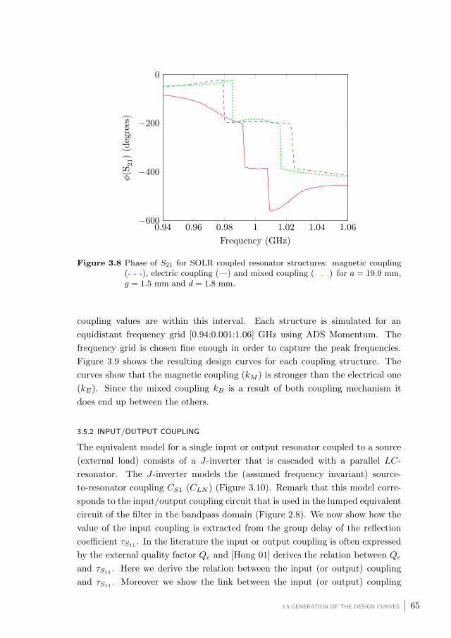
0.94 0.96 0.98 1 1.02 1.04 1.06−600

−400

−200

0

Frequency (GHz)

φ(S

21)

(deg

rees

)

Figure 3.8 Phase of S21 for SOLR coupled resonator structures: magnetic coupling(- - -), electric coupling (—) and mixed coupling (. . .) for a = 19.9 mm,g = 1.5 mm and d = 1.8 mm.

coupling values are within this interval. Each structure is simulated for an

equidistant frequency grid [0.94:0.001:1.06] GHz using ADS Momentum. The

frequency grid is chosen fine enough in order to capture the peak frequencies.

Figure 3.9 shows the resulting design curves for each coupling structure. The

curves show that the magnetic coupling (kM ) is stronger than the electrical one

(kE). Since the mixed coupling kB is a result of both coupling mechanism it

does end up between the others.

3.5.2 INPUT/OUTPUT COUPLING

The equivalent model for a single input or output resonator coupled to a source

(external load) consists of a J-inverter that is cascaded with a parallel LC-

resonator. The J-inverter models the (assumed frequency invariant) source-

to-resonator coupling CS1 (CLN ) (Figure 3.10). Remark that this model corre-

sponds to the input/output coupling circuit that is used in the lumped equivalent

circuit of the filter in the bandpass domain (Figure 2.8). We now show how the

value of the input coupling is extracted from the group delay of the reflection

coefficient τS11. In the literature the input or output coupling is often expressed

by the external quality factor Qe and [Hong 01] derives the relation between Qe

and τS11 . Here we derive the relation between the input (or output) coupling

and τS11. Moreover we show the link between the input (or output) coupling


1 1.2 1.4 1.6 1.8 2 2.2 2.4

1

3

5

7

·10−2

d (mm)

k

Figure 3.9 Desgin curves relating the inter-resonator coupling kE for the electric cou-pling (+), kM for the magnetic coupling (o) and kB for the mixed coupling(x) to the design parameter d.

and Qe.

The input reflection coefficient is written as a function of the impedance of the

source ZS = 1GS

and the input impedance ZIN of the filter seen from the source

[Poza 98]:

S11 =ZIN − ZSZIN + ZS

(3.12)

where ZIN = 1YIN

. To determine YIN , we obtain Y1 first. If Y1 is the admittance

of the parallel LC resonator (Figure 3.10) and given the resonant frequency

Ω0 = 1√C′1L

′1

we obtain YIN by transformation through the J-inverter CS1:

Figure 3.10 Lumped-equivalent circuit for a single input/output resonator coupledto the a non-ideal source with admittance GS .


YIN =C2S1

Y1⇒ ZIN = j

C ′1Ω0

C2S1

(Ω

Ω0− Ω0

Ω) (3.13)

If we write Ω = Ω0 + ∆Ω for a frequency that is assumed to lie in the vicinity

of resonance Ω ≈ Ω0, we approximate ( ΩΩ0− Ω0

Ω ) as:

Ω

Ω0− Ω0

Ω=

(Ω + Ω0)(Ω− Ω0)

ΩΩ0

≈ 2Ω∆Ω

ΩΩ0=

2∆Ω

Ω0

(3.14)

If we now introduce (3.13) in (3.12) using the approximation in (3.14), we obtain:

S11 =GSZIN − 1

GSZIN + 1

=j

Ω0C′1GS

C2S1

∆ΩΩ0− 1

jΩ0C′1GSC2S1

∆ΩΩ0

+ 1

=jX − 1

jX + 1=

1−X2

1 +X2− j 2X

1 +X2

(3.15)

where X =C′1GS∆Ω

C2S1

. The phase of S11 is

φ(S11) = arctan−2X

1−X2(3.16)

The group delay τ is defined as [Poza 98]:

τ = − dφdΩ

(3.17)

We now calculate τS11(Ω0) by deriving (3.16) and evaluating it in Ω0. First we

derive (3.16):


τS11= − 1

1 + (−2X)2

(1−X2)2

−2(1−X2)− 2X(−2X)

(1−X2)2

GSC′1

C2S1

=(1−X2)2

(1 +X2)2

−2(1 +X2)

(1−X2)2

GSC′1

C2S1

=1

(1 +X2)2

2GSC′1

C2S1

(3.18)

Since X(Ω0) = 0, we have that:

τS11(Ω0) =

2GSC′1

C2S1

(3.19)

Using (2.38) we have that MS1 = CS1√GSC1

is the input-coupling in the lowpass

domain, where C1 = FBWΩ0

2 C ′1 (2.32). Filling this in (3.19) yields:

M′2S1 = M2

S1FBW =4

Ω0τS11(Ω0)(3.20)

where we define M ′S1 = CS1√GSΩ0C′1

as the input coupling in the bandpass domain.

Equation (3.20) shows again that to de-normalize the input (output) coupling

it must be multiplied by√FBW . Note that in the literature the input/output

coupling is often expressed using the external quality factor QEXT [Macc 08].

In the case when a resonator l is coupled to an external load G0 through a

J-inverter J0l, the external quality factor is defined as

QEXT,l =blG0

J20l

(3.21)

where bl is the susceptance slope parameter of the admittance Yl of the resonator:

bl =1

2

∂ Im(Yl)

∂Ω

∣∣∣∣Ω=Ω0

(3.22)

In the case of the input parallel LC-resonator, bl = b1 = Ω0C′

1. If we now

assume that G0 = GS and J0l = CS1 we have:


QEXT,1 =Ω0C

′

1GSC2S1

= M′2S1 =

1

M′2S1

=Ω0τS11

(Ω0)

4(3.23)

Expression (3.23) corresponds to the expression found in [Hong 01; Swan 07b]

to extract the quality factor starting from the group delay τS11.

We now apply the extraction method to generate design curves for a SOLR

which is fed using a tapped-line.

Tapped-line Feed SOLR example

A SOLR is usually fed using a tapped-line feeding structure, where the position

of the center of the feed line with respect to the center of the resonators labeled

t mainly affects the input coupling [Wong 79] (Figure 3.11). The width of the

feeding line Wfeed is chosen such that the characteristic impedance of the line

corresponds to the impedance of the source (or the load), which in this case is

50 Ω. The corresponding width of the feed line in the example as used earlier

is Wfeed = 1.48 mm. The derivative of the phase of S11 with respect to the

frequency is approximated by the forward numerical differentiation ∆φ∆ω = φ2−φ1

ω2−ω1.

The structures are simulated for the same frequency range as before, which is

[0.94:0.001:1.06] GHz again using ADS Momentum for values of t within the

interval [7.45:0.01:9.45] mm. These values are chosen to make sure that the

desired input (and output) coupling are within this interval. Figure 3.12 shows

τS11for a = 19.9 mm, g = 1.5 mm and t = 7.95 mm. τS11

(Ω0) is 12.7 ns and

Ω0 = 2π109 rads , which makes that M ′S1 = 0.224. Figure 3.13 shows M ′S1 as a

function of t, the coupling between the source and the resonator increases when

t increases, which is expected and is in line with field density and the impedance

along the resonator.

IN

Figure 3.11 Top-view of the layout of a single SOLR fed using a tapped-line feedingstructure. t denotes the distance between the center of the feed line andthe center of the resonator.


0.94 0.96 0.98 1 1.02 1.04 1.062

4

6

8

10

12

Frequency (GHz)

τS

11

(ns)

Figure 3.12 τS11 as a function of frequency for a tapped SOLR structure with a = 19.9mm, g = 1.5 mm and t = 7.95 mm.

7.4 7.8 8.2 8.6 9 9.40.18

0.2

0.22

0.24

0.26

0.28

0.3

0.32

t (mm)

Inp

ut

cou

pli

ng

Figure 3.13 Input/output coupling for a tapped SOLR structure with a = 19.9 mm,g = 1.5 mm and t in the interval [7.45:0.01:9.45] mm.

3.6 Initial Dimensioning of a Single Quadruplet SOLR Filter

In this section we use the design curves generated in Section 3.5.1 to dimension

a fourth order SOLR quadruplet filter. The filter is designed to have a center

frequency fc = 1 GHz, a FBW = 0.05 and a RL = −20 dB and 2 finite TZs at

ω = ±1.4. We first synthesize the ideal coupling matrix in the lowpass domain


using the techniques described in Chapter 2. The ideal N + 2 coupling matrix

is called Mid and is shown below:

Mid =

0 1.0123 0 0 0 0

1.0123 0 0.7787 0 −0.4286 0

0 0.7787 0 0.8612 0 0

0 0 0.8612 0 0.7787 0

0 −0.4286 0 0.7787 0 1.0123

0 0 0 0 1.0123 0

To implement the coupling matrix, it must be de-normalized. Hence, the inter-

resonator coupling must be multiplied by FBW and the input/output couplings

by√FBW yielding:

Mdenorm =

0 0.2263 0 0 0 0

0.2263 0 0.0389 0 −0.0214 0

0 0.0389 0 0.0431 0 0

0 0 0.0431 0 0.0389 0

0 −0.0214 0 0.0389 0 0.2263

0 0 0 0 0.2263 0

(3.24)

In the ideal coupling matrix, the inter-resonator coupling M14 has an opposite

sign to that of the sequential couplings. Therefore we implement M14 using

the electric coupling structure shown in Figure 3.6a. Moreover the couplings

M12 = M34. To impose this equality we then implement these couplings using

a mixed coupling structure (Figure 3.6c). Finally we implement M24 using the

magnetic coupling structure (Figure 3.6b). Figure 3.14 shows the top-view of the

physical layout of the filter. Table 3.1 contains the initial geometrical dimensions

obtained using the design curves. Figure 3.15 shows the magnitude responses

in the bandpass domain for the filter with the initial dimensions. Figure 3.16

compares the simulated response to the ideal one obtained from the coupling

matrix Mid.

Clearly, the filter response is reasonably close to the ideal one, however there is

still an offset and room for improvement. The TZs have a frequency offset and

quality factor shift with respect to the ideal ones, the bandwidth is slightly larger

than the ideal one and not all of the reflection zeros appear. It is not surprising

that response does not perfectly match the ideal response, as the design curves

3.6 INITIAL DIMENSIONING OF A SINGLE QUADRUPLET SOLR FILTER 71

Figure 3.14 Top-view of the layout of a fourth order SOLR quadruplet filter.

Physical design parameter Initial value (mm)wfeed 1.48tin = tout 7.95g1 = g2 = g3 = g4 1.5a 19.9w 1d12 1.45d23 1.75d34 1.45d14 1.45

Table 3.1 Initial values for the physical design parameters of the SOLR quadrupletfilter.

are based on the approximation that does not take into account the effects of

the loading of other resonators on the coupling parameters. Moreover parasitic

couplings may be present in the actual microwave filter. To assess the difference

in some more detail, knowledge about the implemented (actual) coupling matrix

is helpful. It enables a designer to tune or optimize the geometrical parameters

or at least helps to diagnose the source of the error on the implemented coupling

parameters. In the next chapter we will explain how to extract the implemented

coupling matrix starting from the simulated full-wave response. Later we use

this extraction method to optimize the filter response.


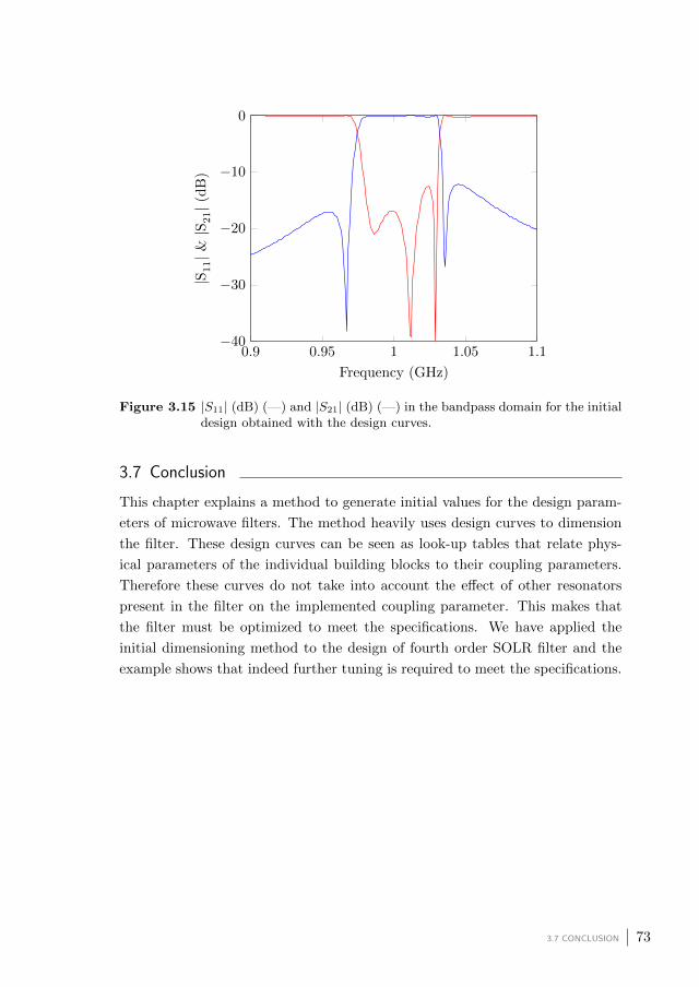
0.9 0.95 1 1.05 1.1−40

−30

−20

−10

0

Frequency (GHz)

|S11|&|S

21|(

dB

)

Figure 3.15 |S11| (dB) (—) and |S21| (dB) (—) in the bandpass domain for the initialdesign obtained with the design curves.

3.7 Conclusion

This chapter explains a method to generate initial values for the design param-

eters of microwave filters. The method heavily uses design curves to dimension

the filter. These design curves can be seen as look-up tables that relate phys-

ical parameters of the individual building blocks to their coupling parameters.

Therefore these curves do not take into account the effect of other resonators

present in the filter on the implemented coupling parameter. This makes that

the filter must be optimized to meet the specifications. We have applied the

initial dimensioning method to the design of fourth order SOLR filter and the

example shows that indeed further tuning is required to meet the specifications.

3.7 CONCLUSION 73

−4 −3 −2 −1 0 1 2 3 4−40

−30

−20

−10

0

ω

|S11|(

dB

)

(a) |S11| (—) for the simulated filter and ideal response (—) and the specifications (-- -).

−4 −3 −2 −1 0 1 2 3 4−40

−30

−20

−10

0

ω

|S21|(

dB

)

(b) |S21| (—) for the simulated filter and ideal response (—) and the specifications (-- -).

Figure 3.16 Comparison between the ideal and simulated response.


4Extraction of the Coupling Matrix

This chapter presents a method to extract a coupling matrix starting from the

simulated (or measured) S-parameters of the filter. The S-parameters are first

transformed to the lowpass domain. The extraction method estimates a common

denominator matrix of prescribed McMillan degree N for the S-parameters of

the filter in the lowpass domain after adjusting the reference plane. Next it

synthesizes a coupling matrix in the arrow form. This coupling matrix is then

reconfigured to match the implemented coupling topology. In the case of multiple

solutions, all admissible solutions are determined. The extraction method has

been implemented in the Matlab toolbox PRESTO-HF [Seyf 04], which we use to

extract the arrow form coupling matrix starting from the simulated S-parameters

of the filter. Since we are dealing with non-ideal (real) filters, the simulated data

do not perfectly match the coupling matrix model. By a real filter, we mean

the electromagnetic model of the filter, and not real in the sense that the filter

is manufactured. This makes that the coupling matrix also contains parasitic

couplings. At the end of this chapter we explain how parasitic couplings are

handled and how this affects the reconfiguration of the coupling matrix. The

coupling matrix extraction method is applied to a single and to a cascaded

quadruplet filter.

4.1 Introduction

In filter design it is necessary to extract the arrow form coupling matrix starting

from the simulated or measured S-parameters of the filter. Knowledge of the

extracted coupling matrix allows a designer to diagnose problems if the imple-

mented coupling matrix is too far a way from the ideal target coupling matrix.

This ideal matrix is also called the golden goal. A designer can then correct or

tune the physical dimensions of the filter to bring the coupling matrix closer to

the target one. To be able to tune the physical dimensions of the filter using the

75

extracted coupling matrix, one must be sure to extract the coupling matrix that

is physically implemented. As we have seen in Section 2.8.3 and Section 3.6,

the implemented coupling topology does not always correspond to the arrow

form. Moreover the implemented topology can have multiple mathematically

equivalent solutions leading to a coupling matrix of the desired form. Another

problem is the presence of parasitic couplings. These second order perturbation

effects change the structure of the coupling matrix, hereby modifying the fre-

quency response function (FRF) in a way that is not contained in the golden

goal. In this chapter we explain how we extract the arrow form coupling matrix

starting from simulated (or measured) S-parameters, to reconfigure it to the

target coupling topology and to handle the presence of parasitic couplings. The

procedure used to handle multiple solutions is discussed in the next chapter.

Over the last years several methods to extract the coupling matrix starting from

the S-parameters have been developed in order to tune filters [Hars 01; Hars 02;

Bila 99; Seyf 03; Garc 04; Lamp 04; Hu 13; Hu 14]. These extraction techniques

can roughly be divided in 2 categories:

• Optimization-based methods optimize the coupling matrix parameters to

fit the measured/simulated S-parameters in the lowpass domain [Hars 01;

Hars 02]. These methods yield only one solution by construction. The

solution strongly depends on the initial values for the coupling parameters

that need to be specified by the user. Only one solution is obtained,

even if there are multiple possibilities. Unfortunately, this one solution

does not necessarily correspond to the physically implemented one. A

comparison based on a coupling matrix that is inconsistent with the actual

filter physical dimensions can propose incoherent corrections destroying the

tuning procedure.

• Network-synthesis-based methods first identify the numerator polynomials

of S11 and S21 [Garc 04; Lamp 04] or a rational matrix [Bila 99; Seyf 03;

Hu 13; Hu 14] representing the measured/simulated S-parameters in the

lowpass domain. Next the method synthesizes a coupling matrix starting

from the identified polynomials or the rational form. In the case of coupling

topologies having multiple solutions these methods do not specify which

solution is synthesized.

Since we want to handle coupling topologies supporting multiple solutions, we

use an extraction method of the second category. The rational approxima-

76 CHAPTER 4 EXTRACTION OF THE COUPLING MATRIX

tion used in this work is described in [Seyf 03; Oliv 13] and is based on H2-

approximation [Marm 02]. This method mainly consists of 2 steps:

1. An analytical completion is obtained first to derive a stable and causal

model of very high degree that fits the data.

2. A rational approximation is pursued next that identifies a stable rational

matrix of an a-priori and imposed McMillan degree N .

The method also takes into account the influence of the presence of feeding

or access lines on the filter response and automatically adjusts the reference

plane. The method has been implemented in the Matlab toolbox PRESTO-HF

[Seyf 04], which we will use intensively in the remainder of this work. Section 4.3

explains the principles used in the rational approximation method. The main

benefit of this method is that it identifies a stable, causal, rational matrix of

fixed MacMillan degree N , where N corresponds to the order of the lowpass

equivalent filter or the number of resonators present in the physical filter. As we

have seen in Section 2.7.2, this is a necessary condition to be able to synthesize

a minimal coupling matrix of size (N + 2)× (N + 2). We now briefly discuss the

differences with the other methods of the second category.

The method described in [Garc 04] is called the Cauchy method. This method

assumes that the Feldtkeller equation (2.17) is valid for the physical filter. The

method first estimates the rational model for the ratio S11

S21. Next it identifies

the numerator of this function as the reflection polynomial and the denominator

as the numerator polynomial of the transmission function. Finally it constructs

the common denominator of the rational S-matrix using the Feldtkeller equa-

tion. One of the drawbacks of this method is that it assumes that the filter

is loss-less, which is not the case in practice. Therefore the method has been

improved to handle lossy data by reformulating the total least-squares problem

without imposing the lossless condition [Lamp 04]. Another approach [Macc 10]

assumes that all of the resonators have the same unloaded quality factor Qu.

This method transforms the S-parameters to a predistorted frequency domain

using the following frequency transformation:

ω =1

FBW(

1

Qu+ j(

f

fc− fcf

)) (4.1)

Next it applies the Cauchy method in the predistorted frequency domain, thereby

avoiding all of the problems related to the synthesis of lossy networks such

4.1 INTRODUCTION 77

as complex couplings. This method heavily relies on the assumption that the

unloaded quality factor is known and equal for all resonators.

The method described in [Hu 13; Hu 14] estimates a rational matrix for the

Y -parameters using the vector fitting (VF) algorithm [Gust 99; Gust 06]. The

VF algorithm estimates a pole-residue form in least-squares sense on the data

by iteratively re-locating the position of the poles. The benefit of the methods

described above is that they are relatively simple to implement and yield accurate

rational models.

The main drawback of the methods described in [Lamp 04; Hu 13; Hu 14] is

the fact that the identified rational matrix is not imposed to have a McMillan

degree N . This is a problem since the methods next synthesize a coupling matrix

using the method described in [Came 03]. This method [Came 03] is equivalent

to Gilbert’s method [Gilb 63] and thus assumes that the rational matrix is of

fixed McMillan degree N (Section 2.7.2). Applying it to a rational form that

is not of McMillan degree N , introduces an error and results in the estimation

of a coupling matrix that does no longer represent the rational S-matrix. Since

the method used here extracts a rational matrix of McMillan degree N , it can

always be used to synthesize the transversal N + 2 coupling matrix.

The transversal N+2 coupling matrix is first transformed to the canonical arrow

form coupling topology. To enable one to transform the arrow form to the target

coupling topology, both coupling matrices have to have the same number of non-

zero elements as is discussed in Section 2.8.3. Since the filter is not ideal, this

compatibility condition is generally not met. In section Section 4.5, we explain

how to reduce the arrow form matrix (remove the parasitic couplings) such that

it can be transformed to the target coupling topology. The transformation is

done using the Matlab toolbox DEDALE-HF [Seyf 00]. In the case of multiple

solutions, we determine all possible solutions. How to identify the physical

solutions in this set of possibilities is discussed in the next chapter. Section 4.6

explains how the parasitic couplings are taken into account and how they should

be interpreted. Finally the extraction method is applied to two examples: a

single and a cascaded quadruplet filter.

A limitation of the proposed extraction technique is that the model order must

be the same of the synthesized filter N . In the physical device the actual order

is however higher, due to the frequency variation of the couplings, higher order

mode resonances, etc. The effect of these inaccuracies can not be compensated

by including spurious couplings, since this modifies only the number of zeros nfz

as is explained in Section 2.8.


In what follows we first explain how the data is transformed to the lowpass

domain, next the rational approximation and finally the synthesis of the coupling

matrix having the desired coupling topology. Note that Section 4.3 can be seen

as a summary of [Oliv 13] and [Seyf 03].

4.2 Bandpass-to-Lowpass Transformation

The simulated or measured frequencies are transformed to the lowpass domain

using the following transformation:

ωi =2

f2 − f1(fi − f0) =

2

Ω0FBW(Ωi − Ω0) (4.2)

where fi is a simulated frequency in the bandpass domain and ωi is the corre-

sponding normalized frequency in the lowpass domain and Ω is the bandpass

angular frequency. f0 is the center frequency and f1 and f2 are the cut-off fre-

quencies of the passband specified by the frequency template. Since the center

frequency f0 and fractional bandwidth FBW of the filter to be optimized are

not necessarily equal to the ideal f0 and FBW , the passband of the simulated

S-parameters in the lowpass domain does not always lie between [-1,1]. Note

that the transformation given in (4.2) is the same as the one used in Section 2.5

to transform the lumped-equivalent network to the lowpass domain (2.30).

4.3 Rational Approximation and Reference Plane Adjustment of theS-parameters

The extraction method identifies a mathematical model for the simulated S-

parameters of the filter in the lowpass domain:

SSim(jωi) =

[SSim11

(jωi) SSim12(jωi)

SSim21(jωi) SSim22

(jωi)

](4.3)

where i ∈ 1, . . . , nF and nF denotes the number of simulated frequencies. The

mathematical model is denoted as H and has the following form:

H(jω) =1

q(jω)

[e−j(ωα11+β11)p11(jω) e−j(ω

α11+α222 +

β11+β222 )p12(jω)

e−j(ωα11+α22

2 +β11+β22

2 )p21(jω) e−j(ωα22+β22)p22(jω)

]

(4.4)

4.2 BANDPASS-TO-LOWPASS TRANSFORMATION 79

where q is the common denominator polynomial of order N and p11, p12, p21

and p22 are the numerator polynomials of order N . α11 and α22 are real-valued

constants that model the delays introduced by the access (feeding) lines at in-

put and output respectively. β11 and β22 are real-valued constants that model

the frequency shift introduced by the bandpass-to-lowpass transformation (4.2).

Note that (4.4) can also be written as:

[e−j(ωα11+β11) 0

0 e−j(ωα22+β22)

]Srat(jω)

[e−j(ωα11+β11) 0

0 e−j(ωα22+β22)

](4.5)

where the first and last matrix model the access lines and the matrix Srat(jω)

models the filter. The coupling matrix is synthesized starting from the stable

rational matrix Srat of McMillan degree N :

Srat(jωi) =1

q(jωi)

[p11(jωi) p12(jωi)

p21(jωi) p22(jωi)

](4.6)

To have a stable rational approximation of good quality, the algorithm requires

that the S-parameters are known at each frequency ranging from −∞ to +∞(∀ω ∈ R). Therefore the identification method first computes a stable and causal

model of high degree starting from the simulated S-parameters with the delays

removed, this step is called the completion stage. This high degree model thus

describes the behavior of the filter (without access lines) in the lowpass domain

for all frequencies going from −∞ to +∞. Next the rational matrix (of much

lower degree N) is estimated by rational H2 approximation using the high degree

model as an input [Oliv 13; Marm 02].

The method to identify the mathematical model given in (4.4) starting from sim-

ulated S-parameters of the filter in the lowpass domain consists of the following

steps:

1. Completion:

• Estimation of the delays α11 and α22.

• Analytic completion of the simulated S-parameters with delays re-

moved

• Estimation of the frequency shifts β11 and β22.


2. Estimation of the rational matrix Srat starting from the analytic comple-

tion.

4.3.1 DELAY ESTIMATION

The estimation of α11 and α22 relies on the hypothesis that the rational behavior

in (4.4) for frequencies far from the passband are well approximated by the first

few terms of their Taylor expansion at infinity [Seyf 03]. This boils down to

assuming that the rational model of the filter behaves as a low degree polynomial

in 1ω for frequencies far out the passband. To be able to estimate the delays,

the filter must therefore be simulated over a broader frequency band than the

passband of the filter. Consider only the simulated frequencies that are smaller

than −ωc and larger than ωc with |ωc| > 1:

I = ωi, |ωi| ≥ ωc (4.7)

The value of α11 is found by minimizing the least-squares cost function ψ:

ψ(αl) = min(a0,a1,...,anm−1)∈C(nc−1)

∑

ωi∈I

∣∣∣∣nm−1∑

k=0

akωki− SSim11(ωi)e

jωiαl

∣∣∣∣2

(4.8)

For a fixed value of αl, ψ(αl) is minimized in least-squares sense over the coeffi-

cients (a0, a1, . . . , anm−1) ∈ C(nm−1). Since the value of α11 corresponds to the

physical delay, it is possible to determine boundaries for the interval in which α11

is located based on the geometry of the circuit. The function ψ is exhaustively

searched within this interval with a prescribed tolerance on αl. α11 is determined

as the value for which ψ is minimal within the interval.

To determine α22 we proceed in the same way using SSim22instead of SSim11

.

Once α11 and α22 are estimated, we de-embed the delays of simulated S-parameters

as follows:

SCa(jωi) =

[ejωiα11SSim11(jωi) ejωi

α11+α222 SSim12(jωi)

ejωiα11+α22

2 SSim21(jωi) ejωiα22SSim22(jωi)

](4.9)

4.3 RATIONAL APPROXIMATION AND REFERENCE PLANE ADJUSTMENT OF THE S-PARAMETERS 81

4.3.2 ANALYTIC COMPLETION

The completion stage computes a stable and causal high degree order model F

for the de-embedded S-parameters for all frequencies going from −∞ to +∞.

The model is computed starting from the de-embedded S-parameters at the sim-

ulated frequencies in the lowpass domain. The frequency interval corresponding

to the simulated frequency band is denoted as:

J = [min(ωi),max(ωi)] (4.10)

where ωi denotes a simulated frequency in the lowpass domain. For a value

between 2 simulated frequencies SCa is computed by spline interpolation. We

denote the complement of the interval J as:

Jc =]−∞,min(ωi)[ ∪ ] max(ωi),+∞[ (4.11)

We split the frequency span −∞ ≤ ω ≤ +∞ in the partition of J and Jc. For

frequencies in Jc, we model the S-parameters using a low degree polynomial mkl

in 1ω using the same assumption as in Section 4.3.1. SCakl(jω) (the elements

of the matrix SCa labeled k, l ∈ 1, 2) represents the function in J , while

the polynomial mkl(jω) is used for frequencies in Jc. The complete function is

labeled as SCakl(jω)∧mkl(jω). In order to determine mkl we use a cost function

as in (4.8) to estimate the coefficients of mkl(jω), but we also take into account

that F must be causal and stable. Since we want to obtain a stable, causal and

rational model Srat, we first want to have a stable high-order model to prepare

the rational approximation step.

For a rational model the stability and causality properties require that all the

poles are finite and in the open left half plane. The latter is equivalent to the

fact that the function is analytic in the closed right half plane and at infinity.

To properly handle these properties mathematically we embed the rational func-

tions in a larger space of functions which are known to be analytic in the right half

plane: the Hilbert space of analytic functions in the open right half plane. Their

L2(dµ(ω))-norm remains uniformly bounded on vertical lines [Seyf 03; Part 97]

whenever dµ(ω) = dω1+ω2 . This space is a Hardy space of the right half plane and

we denote it as H2µ. The L2(dµ(ω))-norm of a function f is given by:

‖ f ‖2=

∫ +∞

−∞

|f(jω)|21 + ω2

dω (4.12)


We define L2µ as the space of all complex functions defined on the imaginary axis

for which (4.12) is finite. H2µ can be viewed as a subspace of the space L2

µ. If we

define G2µ as the orthogonal complement of H2

µ in L2µ every function f ∈ L2

µ can

be written as the sum of a function in H2µ (the stable part) and a function in G2

µ

(the unstable part) [Seyf 03]. We denote PH2µ(f) as the orthogonal projection

of f on H2µ and similarly PG2

µ(f) as the orthogonal projection of f on G2

µ. This

framework provides us with an interesting tool to estimate the stability and

causality of a function.

The following minimization problem is solved to determine the polynomials

mkl(jω) (k, l ∈ 1, 2):

minmkl

∑

ωi∈I

∣∣∣∣SCakl(jωi)−mkl

(1

jωi

) ∣∣∣∣2

(4.13)

with

mkl ∈ Cnm [X]

‖ PG2µ(SCakl ∧mkl) ‖2≤ Ec

∀ω ∈ Jc, |mkl|2 ≤ 1

(4.14)

Herein PG2µ(SCakl ∧ mkl) is the projection of the completed data on G2

µ and

represents the unstable part of the completed data. Cnc [X] denotes the set of

polynomials with complex coefficients whose degree is smaller or equal to nm. Ec

is an upper bound on the norm of the unstable part of the completed data. The

last expression in (4.14) is an upper bound on the magnitude of the completed

data in Jc, which must be smaller than 1 for ωi ∈ Jc. This optimization problem

has a unique solution unless the set of admissible solutions is empty, hence it is

a convex problem [Seyf 03].

The completed S-matrix is given by:

SCb(jω) =

[(SCa11

∧m11)(jω) (SCa12∧m12)(jω)

(SCa21∧m21)(jω) (SCa22

∧m22)(jω)

](4.15)

Novel approach

In the latest version of PRESTO-HF [Seyf 04], the completion is performed

simultaneously with the determination of the delay τ . We associate a polynomial

pτ to a delay τ where pτ is the minimizer of:

4.3 RATIONAL APPROXIMATION AND REFERENCE PLANE ADJUSTMENT OF THE S-PARAMETERS 83

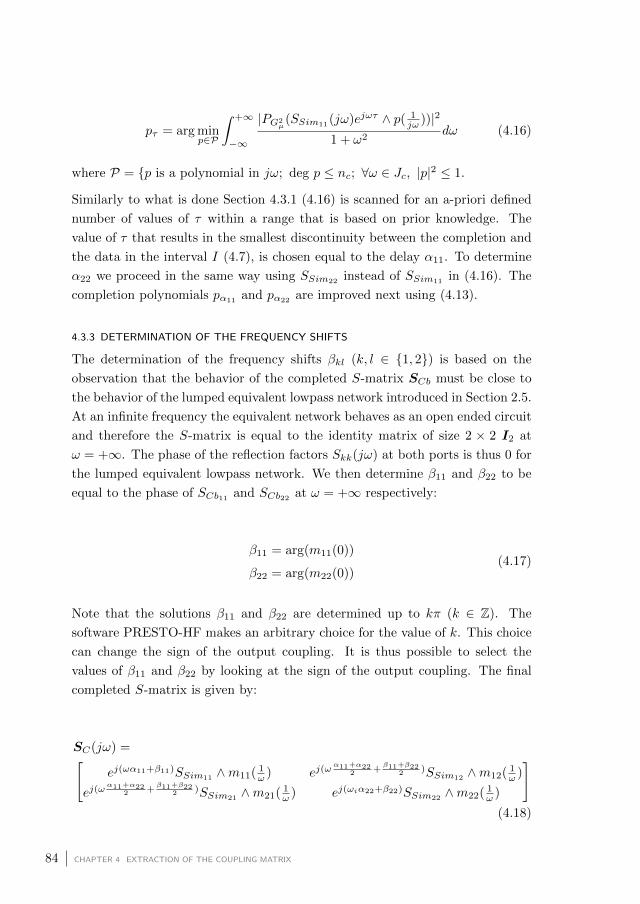
pτ = arg minp∈P

∫ +∞

−∞

|PG2µ(SSim11(jω)ejωτ ∧ p( 1

jω ))|21 + ω2

dω (4.16)

where P = p is a polynomial in jω; deg p ≤ nc; ∀ω ∈ Jc, |p|2 ≤ 1.

Similarly to what is done Section 4.3.1 (4.16) is scanned for an a-priori defined

number of values of τ within a range that is based on prior knowledge. The

value of τ that results in the smallest discontinuity between the completion and

the data in the interval I (4.7), is chosen equal to the delay α11. To determine

α22 we proceed in the same way using SSim22instead of SSim11

in (4.16). The

completion polynomials pα11and pα22

are improved next using (4.13).

4.3.3 DETERMINATION OF THE FREQUENCY SHIFTS

The determination of the frequency shifts βkl (k, l ∈ 1, 2) is based on the

observation that the behavior of the completed S-matrix SCb must be close to

the behavior of the lumped equivalent lowpass network introduced in Section 2.5.

At an infinite frequency the equivalent network behaves as an open ended circuit

and therefore the S-matrix is equal to the identity matrix of size 2 × 2 I2 at

ω = +∞. The phase of the reflection factors Skk(jω) at both ports is thus 0 for

the lumped equivalent lowpass network. We then determine β11 and β22 to be

equal to the phase of SCb11and SCb22

at ω = +∞ respectively:

β11 = arg(m11(0))

β22 = arg(m22(0))(4.17)

Note that the solutions β11 and β22 are determined up to kπ (k ∈ Z). The

software PRESTO-HF makes an arbitrary choice for the value of k. This choice

can change the sign of the output coupling. It is thus possible to select the

values of β11 and β22 by looking at the sign of the output coupling. The final

completed S-matrix is given by:

SC(jω) =[

ej(ωα11+β11)SSim11 ∧m11( 1ω ) ej(ω

α11+α222 +

β11+β222 )SSim12 ∧m12( 1

ω )

ej(ωα11+α22

2 +β11+β22

2 )SSim21∧m21( 1

ω ) ej(ωiα22+β22)SSim22∧m22( 1

ω )

]

(4.18)


The matrix SC models the de-embedded behavior of the filter data for −∞ ≤ω ≤ +∞. The projection of SC on H2

µ is F . The matrix F is the starting point

for the rational approximation Srat.

4.3.4 DETERMINATION OF STABLE RATIONAL MATRIX OF MCMILLAN DEGREE N

Knowing the delays αii, the frequency shifts βii and the polynomials mkl that

complete the S-parameters outside of the simulated frequency band, we can

finally define the matrix F :

F (jω) =

[PH2(SC11)(jω) PH2(SC12)(jω)

PH2(SC21)(jω) PH2(SC22)(jω)

](4.19)

The matrix F (jω) represents the stable part of the filter response with the

influence of the access lines de-embedded for every lowpass frequency in the range

from −∞ to +∞. The rational matrix Srat(jω) is determined by minimizing

the following least-squares approximation problem:

minR‖ F (jω)−R(jω) ‖2=

∑

k,l∈1,2‖ Fkl(jω)−Rkl(jω) ‖2 (4.20)

where R(jω) is a stable rational matrix of McMillan degree ≤ N . The minimizer

of (4.20) is called Srat(jω). The problem (4.20) is minimized using the software

RARL2 [RARL] . Without going into detail, we mention that the algorithms

implemented in RARL2 [RARL] are based on the following principles:

• The stable rational matrices of given McMillan degree can be nicely parametrized

using Schur parameters.

• If Fkl 6∈ H2, the unstable part of Fkl can not be well approximated by a

stable rational function Rkl.

More details can be found in [Oliv 13; Marm 02].

4.4 Synthesis of the Coupling Matrix in Arrow Form

The coupling matrix extraction yields a transversal N +2 coupling matrix start-

ing from the rational matrix Srat(jω) using Gilbert’s method [Gilb 63] (Sec-

tion 2.7.2). Next, this matrix is transformed to its canonical arrow form M0arr

(Section 2.7.3). The rational approximation method imposes the causality, the

4.4 SYNTHESIS OF THE COUPLING MATRIX IN ARROW FORM 85

stability and the McMillan degree N of Srat(jω). The latter is a necessary

condition to obtain a state-space system matrix of size N ×N (Section 2.7.2) as

is required here.

The rational approximation does not impose the order of p21(jω) and therefore

it normally identifies N finite transmission zeros. This implies that a direct

source-to-load coupling is to be present in the extracted N + 2 coupling matrix.

This can be shown using the shortest path rule that is explained in Section 2.8.1.

The corresponding rational Y -parameters hence do not fulfill (2.78), as the num-

ber of transmission zeros exceeds N−2. (2.78) is a necessary condition to obtain

a matrix Bf where only elements (1, 1) and (N, 2) are non-zero as is explained in

(2.91). These elements represent the source-to-resonator 1 and load-to-resonator

N coupling respectively. When the number of transmission zeros exceeds N −1,

the elements (1, 2) and (N, 1) of Bf are also non-zero. The elements (1, 2)

and (N, 1) represent the load-to-resonator 1 and source-to-resonator N coupling

respectively.

The fact that the number of transmission zeros exceeds N − 2, also results

in a non-zero arrow form where the main diagonal, first upper diagonal and

last column are obtained as is explained in Section 2.8.2. This implies that

the presence of more inter-resonator couplings in the simulated filter than in

the ideal coupling topology. These couplings can be interpreted as parasitic

or unwanted couplings. The non-zero diagonal elements can be interpreted as

frequency offsets between the resonant frequency of the individual resonators

and the center frequency of the filter.

Note that the simulated filter is not necessarily lossless. In the case of a lossy

structure the elements of the coupling matrix are complex rather than purely

imaginary. The real part of the diagonal elements can be interpreted as the

quality factor of the resonators (Section 2.6.1). Although synthesis methods

exist that take into account lossy couplings [Mira 08], we do not take them into

account here neither during the synthesis or the tuning of the filter.

The extraction method yields a complex-valued arrow form coupling matrix

M0arr where the diagonal, first upper diagonal and last column are non-zero.

This is not in line with the arrow form obtained from the golden goal and

therefore additional steps are needed to bring the 2 representations as closely

together as possible in order to be able to reconfigure the extracted matrix to

the coupling topology of the golden goal.


4.5 Reconfiguration of the Extracted Arrow Form Matrix

The extracted arrow form M0arr is in general not compatible with the ideal

coupling topology of the prototype filter, since its number of non-zero elements

exceeds the number of degrees of freedom that can be accommodated by the

target topology (Section 2.8.2). As seen in Section 4.4, this is due to the presence

of parasitic couplings.

Some of these couplings can be seen as second order effects that influence the

filter only marginally, but unfortunately some others must be treated as first

order effects with a significant impact. In what follows we describe the coupling

topology of a filter by means of a matrix T whose elements are 1 if the corre-

sponding coupling is present in the topology and are 0 otherwise. As is explained

in Section 2.8.2 a full arrow form is not always compatible with any topology T .

We denote the arrow form that is compatible with a topology T as MTarr. In

order to obtain a compatible arrow form, certain elements of the extracted arrow

form matrix M0arr must be forced to zero, yielding a reduced arrow form MT

arr

of the initial coupling matrix M0arr. We denote the ideal coupling topology of

the golden goal as Tid. We explain in the next section that the coupling topology

of the real filter denoted as Tstruct does not necessarily correspond to Tid.

Reduction of M0arr to MT

arr

To be able to reduce the complete arrow form Marr to the reduced one that is

compatible with the selected physical filter structure MTarr, we need to assume

that the implemented coupling topology is sufficiently close to the ideal topology

Tid. This assumption implies that the elements that are set to zero during the

reduction of the arrow form are small with respect to the elements that are kept.

In other words, we assume that the parasitic inter-resonator couplings are second

order effects. In practice we observe that the parasitic couplings are at least an

order of magnitude lower than the desired couplings.

For topologies supporting asymmetrical responses the matrix M0arr is reduced

to an arrow form MTidarr by simply eliminating the undesired parasitic couplings

in M0arr. In practice this corresponds to eliminating elements in the last row

and column M0arr as is explained in Section 2.8.2. Physically, this eliminates

the couplings that are present in the real filter, but not in the ideal coupling

topology.

For topologies supporting symmetrical responses, the diagonal of Tid is zero and

the diagonal of the corresponding arrow form is to be zero as well. Since the real

physical filter is never perfectly tuned, its response is not ideally symmetrical

4.5 RECONFIGURATION OF THE EXTRACTED ARROW FORM MATRIX 87

with respect to the center frequency. This asymmetry is mainly due to the

presence of self-couplings. Unlike the inter-resonator parasitic couplings, these

self-coupling can not be treated as a second order effects. Therefore they have

to remain present in the reduced arrow form as well. We do not eliminate the

diagonal elements of M0arr by bluntly setting them to zero. We reduce M0

arr to

an arrow form compatible with the coupling topology closest to the ideal coupling

topology that accommodates asymmetric responses instead. This makes that

the coupling topology Tstruct to which the coupling matrix is reconfigured does

not correspond to Tid in this case. This is different in the case for topologies

supporting asymmetrical responses. The choice of the coupling topology Tstruct

heavily depends on the topology Tid. In the examples considered in this work,

we see that Tstruct has a non-zero diagonal and some extra cross-couplings with

respect to Tid. We illustrate this for a cascaded quadruplet filter in Section 4.8.

Note that the number of non-zero couplings grows fromN+nf2

2 +1 to 2N+nfz+1

as is explained in Section 2.8.2.

Reconfiguration of MTarr

OnceMTarr is determined, we calculate all the similarity transformation matrices

Pi that reconfigure MTarr to the desired coupling topology T . These similarity

transformations are obtained using the software DEDALE-HF [Seyf 00]. Note

that nS multiple solutions might exist for certain coupling topologies. (nS de-

notes the number of solutions) For such topologies every possible solution (every

possible transformation Pi (i ∈ 1, . . . , nS)) is determined. Once every Pi is

determined, they are applied to the originally extracted arrow form coupling ma-

trix M0arr. We apply the transformation to M0

arr rather than MTarr, to take into

account the second order parasitic couplings. This process yields nS extracted

coupling matrices MPi (i ∈ 1, . . . , nS). Note that these matrices still contain

non-zero elements in their last column (and last row) that are not present in the

ideal topology. This step thus re-introduces the parasitic couplings that were

eliminated to obtain MTarr.

4.6 Dealing with Parasitic Couplings

As is explained in Section 2.8.3, the matrices MPi (i ∈ 1, . . . , nS) contain non-

zero elements resulting in couplings that are not present in the ideal coupling

topology. These non-zero elements are located in the last column and row ofMPi

and are therefore not necessarily located at the place where they are physically

expected. These elements can be interpreted as follows: they model the part of

the filter response that can not be explained (modeled) by the coupling matrix


model of the ideal coupling topology. They do not only model the effect of the

parasitic couplings, but can also account for the fact that the physical coupling

is not frequency independent while this is assumed in the coupling matrix model.

In order to have a more physical distribution of the parasitic couplings, we can

approximate the compensated simulations SC(jω) at the simulated lowpass fre-

quencies by a coupling matrix that contains non-zero elements only at positions

where the parasitic couplings are expected to be present from a physical point

of view. The initial matrix that is used to start this optimization method is

the matrix MPi in which the extra elements in the last row and column are

removed. We denote this matrix as Mpar,0 . Eliminating elements in the last

row and column, will for sure deteriorate the approximation. The idea is to add

the parasitic couplings in the matrix to improve the approximation. Therefore

the optimization method minimizes the 2-norm of the difference between the

compensated S-matrix and the response created by the coupling matrix. For

each S-parameter the method calculates the 2-norm of the difference between

SCkl(jω) and the response created by Mpar,h (where h denotes the iteration in

the optimization method):

ckl =

√√√√nf∑

f=1

|SCkl(ωf )− SMpar,h

kl (ωf ))|2 (4.21)

where k, l ∈ 1, 2, nf is the number of simulated frequencies and SMpar,h

kl is the

response corresponding to the coupling matrix Mpar,h.

The least-squares cost function that is minimized is the 2-norm of the total

difference:

c =

√√√√2∑

k=1

2∑

l=1

c2kl (4.22)

and is to be minimized over the non-zero elements in the coupling matrixMpar,h.

The minimizer is calculated using the Matlab function fminunc, which searches

the minimum for an unconstrained multi-variable scalar function. The drawback

of this method is that it heavily depends of its initial values and that the algo-

rithm might converge to a local minimum of unpredictable quality if the initial

value is poor. In Section 4.8 we apply this optimization method to redistribute

the parasitic couplings in cascaded quadruplet topology.

4.6 DEALING WITH PARASITIC COUPLINGS 89

4.7 Example: Single Quadruplet (SQ) Filter

We now apply the coupling matrix extraction method to the single quadru-

plet square open-loop resonator filter introduced in Section 3.6. The prescribed

McMillan degree of the lowpass filter is 4. The filter is simulated for [0.9:0.001:1]

GHz. The ideal center frequency and fractional bandwidth for which the filter

is designed, are fc = 1 GHz and FBW = 0.05 respectively. The corresponding

lowpass frequency grid is calculated to be [-4:0.04:4]. The extracted values for the

delays and the frequency shifts are grouped in the matrices α and β respectively:

α =

[0.0580 0.0585

0.0585 0.059

]β =

[−2.8491 0.3158

0.3158 −2.8494

](4.23)

Figure 4.1 compares the simulated response SSim11to the completed data SC11

and the rational approximation SRat11 and SSim21 to SC21 and SRat21 for the

simulated frequencies in the lowpass domain. It can be observed that there is a

difference in phase between SSim11and SC11

and between SSim21and SC21

, due

to the de-embedding of the access lines. Figure 4.2a compares the magnitude

of to |SC11| and |SRat11

| and shows the magnitude of the approximation error

|SRat11−SC11

|. Figure 4.2b compares the magnitude of to |SC21| and |SRat21

| and

shows the magnitude of the approximation error |SRat21 − SC21 |. Both figures

show that Srat approximates the data well, especially in the passband. Figure 4.3

shows the results given by PRESTO-HF. The red curve is the completed data

SC . The number r expresses the ratio between the norm of the unstable part

of the data (PG2(SCkl), k, l ∈ 1, 2) and the norm of the (unprojected) data

(SCkl), k, l ∈ 1, 2). It is clear that the unstable part is much smaller than the

stable part: r ≤ 0.53% for each S-parameter, which clearly indicates that the

assumption that the filter is a stable device holds. The blue curve is the rational

approximation Srat. The number err expresses L2-norm of the relative error

and err.sup the L∞-norm of the relative error. The rational approximations

have very low relative errors which implies that the model fits the data well.

This is also expected since the physical filter is narrow-banded and the number

of resonators present is equal to the chosen McMillan degree, namely 4. This

indicates that the behavior of the physical filter can be modeled well using a

lumped-equivalent network.

Figure 4.4 shows the pole-zero map of Srat21, there are 4 transmission zeros. 2

of them are almost purely imaginary, which is expected from the ideal coupling


−1 −0.5 0 0.5 1−1

−0.5

0

0.5

1

Real part S11

Imag

inar

yp

art

S11

(a) Nyquist diagram for SSim11 (–o), SC11 (–o) and SRat11 (–+).

−1 −0.5 0 0.5 1−1

−0.5

0

0.5

1

Real part S21

Imag

inar

yp

art

S21

(b) Nyquist diagram for SSim21 (–o), SC21 (–o) and SRat21 (–+).

Figure 4.1 Comparison between the simulations, analytic completion and rationalapproximation for S11 and S21.

topology. While the other 2 are complex and relatively far from the passband,

which makes that the direct source-to-load coupling is not that strong as we will

see in the extracted coupling matrix. Note that there are 2 poles that do not

lie in the passband, which is consistent with the fact that the bandwidth of the

physical filter is broader than the desired bandwidth.

4.7 EXAMPLE: SINGLE QUADRUPLET (SQ) FILTER 91

−4 −3 −2 −1 0 1 2 3 4−80

−70

−60

−50

−40

−30

−20

−10

0

ω

|S11|(

dB

)

(a) Magnitude of |SC11 | (–o), |SRat11 | (–+) and the approximationerror (x).

−4 −3 −2 −1 0 1 2 3 4−90

−80

−70

−60

−50

−40

−30

−20

−10

0

ω

|S21|(

dB

)

(b) Magnitude of |SC21 | (–o), |SRat21 | (–+) and the approximationerror (x).

Figure 4.2 Comparison between the magnitude of the analytic completion and ratio-nal approximation for S11 and S21 and the error of the approximation.

Figure 4.5 compares the coupling graphs of the ideal SQ filter and the coupling

graph of the extracted arrow form M0arr.


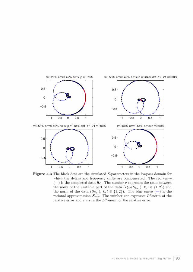
−1 −0.5 0 0.5 1

−0.5

0

0.5

r=0.29% err=0.42% err.sup =0.76%

−1 −0.5 0 0.5 1

−0.5

0

0.5

r=0.53% err=0.49% err.sup =0.84% diff−12−21 =0.00%

−1 −0.5 0 0.5 1

−0.5

0

0.5

r=0.53% err=0.49% err.sup =0.84% diff−12−21 =0.00%

−1 −0.5 0 0.5 1

−0.5

0

0.5

r=0.50% err=0.54% err.sup =0.90%

Figure 4.3 The black dots are the simulated S-parameters in the lowpass domain forwhich the delays and frequency shifts are compensated. The red curve(—) is the completed data SC . The number r expresses the ratio betweenthe norm of the unstable part of the data (PG2(SCkl), k, l ∈ 1, 2) andthe norm of the data (SCkl), k, l ∈ 1, 2). The blue curve (—) is therational approximation Srat. The number err expresses L2-norm of therelative error and err.sup the L∞-norm of the relative error.


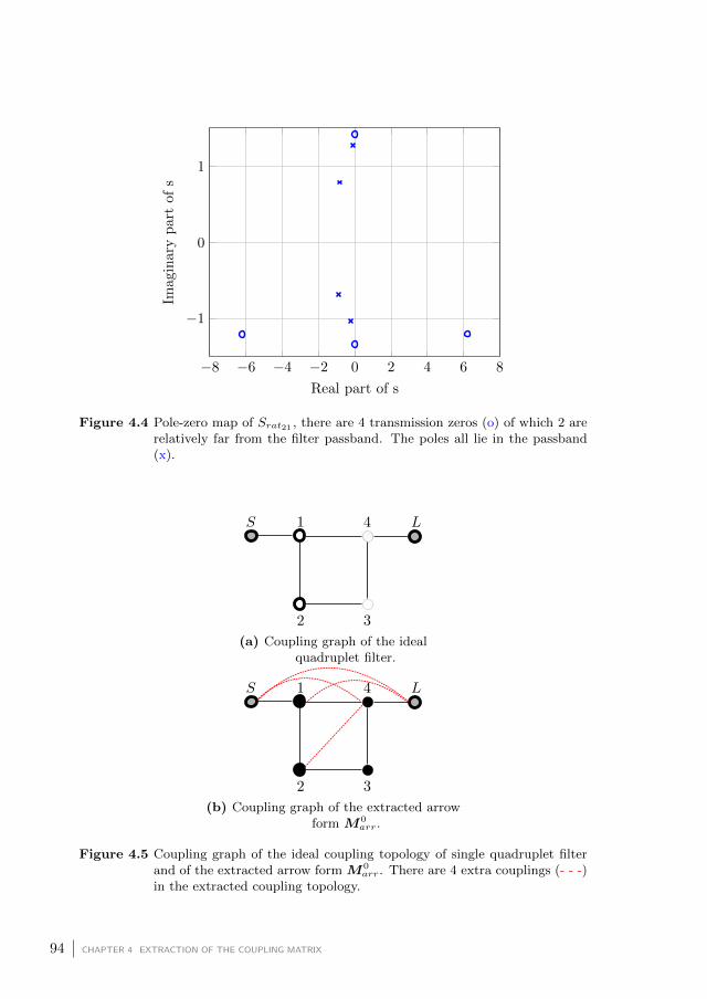
−8 −6 −4 −2 0 2 4 6 8

−1

0

1

Real part of s

Imag

inar

yp

art

ofs

Figure 4.4 Pole-zero map of Srat21 , there are 4 transmission zeros (o) of which 2 arerelatively far from the filter passband. The poles all lie in the passband(x).

(a) Coupling graph of the idealquadruplet filter.

(b) Coupling graph of the extracted arrowform M0

arr.

Figure 4.5 Coupling graph of the ideal coupling topology of single quadruplet filterand of the extracted arrow form M0

arr. There are 4 extra couplings (- - -)in the extracted coupling topology.


The imaginary part of the extracted arrow form matrix is:

Im(M0arr) =

0 1.0228 0 0 0.0131 0.0115

1.0228 0.0266 0.7715 0 −0.4555 −0.0131

0 0.7715 −0.0097 0.8366 0.1845 0

0 0 0.8366 −0.4123 0.7501 0

0.0131 −0.4555 0.1845 0.7501 0.0266 −1.0240

0.0115 −0.0131 0 0 −1.0240 0

(4.24)

Clearly, the extracted coupling matrix contains more non-zero elements than the

ideal coupling matrix given by (3.24) (Figure 4.5). In this particular case the

arrow form topology is very close to the ideal topology of the single quadruplet.

Note that the elements in bold font correspond to the non-zero elements of the

ideal topology. Therefore it is unnecessary to reconfigure M0arr. Also note that

in the case of a single quadruplet filter, there is only one solution to the coupling

matrix reconfiguration problem.

As discussed in Section 4.4, the extracted coupling matrix contains a source-to-

load coupling MSL = 0.0115, a source-to-resonator N coupling MSN = 0.0131

and load-to-resonator 1 coupling ML1 = −0.0131. These couplings are 2 orders

of magnitude lower than the input and output coupling MS1 = 1.0228 and

MLN = −1.0240, which confirms that these additional terms are second order

effects. Also remark that MLN has a negative sign. This is due to the choice of

β21 as is discussed in Section 4.3.3. From a physical point of view MLN should

have the same sign as MS1. It is possible to redo the extraction procedure with

a different choice for β21. In this case we did not have to do this, because this

choice does not affect the values of the coupling parameters.

Another notable difference is the presence of the self-couplings, which also ex-

plains why the center frequency of the passband of the filter does not exactly

coincide with 1 GHz of the prototype filter (as can be seen in Figure 3.16). Fi-

nally there is M24 which models the presence of a parasitic coupling. Although

M24 is smaller than the other inter-resonator couplings, it is still of the same

order of magnitude indicating that the presence of the parasitic couplings is

not negligible. From a physical point of view there is no reason to assume the

presence of coupling M24 and the absence of the coupling M13. It is possible to

re-optimize the coupling matrix to redistribute the parasitic couplings in a more


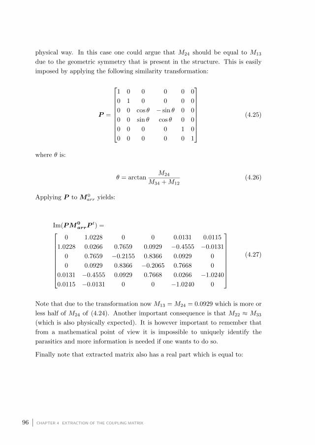
physical way. In this case one could argue that M24 should be equal to M13

due to the geometric symmetry that is present in the structure. This is easily

imposed by applying the following similarity transformation:

P =

1 0 0 0 0 0

0 1 0 0 0 0

0 0 cos θ − sin θ 0 0

0 0 sin θ cos θ 0 0

0 0 0 0 1 0

0 0 0 0 0 1

(4.25)

where θ is:

θ = arctanM24

M34 +M12(4.26)

Applying P to M0arr yields:

Im(PM0arrP

t) =

0 1.0228 0 0 0.0131 0.0115

1.0228 0.0266 0.7659 0.0929 −0.4555 −0.0131

0 0.7659 −0.2155 0.8366 0.0929 0

0 0.0929 0.8366 −0.2065 0.7668 0

0.0131 −0.4555 0.0929 0.7668 0.0266 −1.0240

0.0115 −0.0131 0 0 −1.0240 0

(4.27)

Note that due to the transformation now M13 = M24 = 0.0929 which is more or

less half of M24 of (4.24). Another important consequence is that M22 ≈ M33

(which is also physically expected). It is however important to remember that

from a mathematical point of view it is impossible to uniquely identify the

parasitics and more information is needed if one wants to do so.

Finally note that extracted matrix also has a real part which is equal to:


Re(M0arr) =

0 −0.0001 0 0 −0.0002 −0.0016

−0.0001 0.0024 0.0009 0 0.0004 0.0002

0 0.0009 −0.0007 0.0014 0.0005 0

0 0 0.0014 −0.0004 0.0008 0

−0.0002 −0.0004 0.0005 0.0008 0.0023 0.0001

−0.0016 0.0002 0 0 0.0001 −0.0004

(4.28)

Although the filter is simulated for a loss-less substrate and a perfect conductor,

Momentum takes into account the radiation effects. These losses are however

small and can be neglected, as it is seen that the real part is 3 orders of magnitude

smaller than the imaginary part.

4.8 Example: Cascaded Quadruplet (CQ) Filter

For the second example, we apply the extraction method to the design of an 8-

pole cascaded quadruplet (CQ) filter consisting of SOLR resonators (Figure 4.6).

The filter is implemented in a RT/duroid substrate with a relative dielectric

constant εr = 10.2 and a thickness t = 1.27 mm. The filter is designed to

have a center frequency fc = 1 GHz, a FBW = 0.06 and a RL = −23 dB and

2 pairs of finite TZs at ω = ±1.2 and ω = ±1.6. We first synthesize the ideal

coupling matrix in the lowpass domain using the techniques described in Chapter

2. DEDALE-HF [Seyf 00] yields 2 possible solutions for this case, among which

one is chosen. Table 4.1 contains the ideal lowpass coupling parameters. Since

this topology accommodates a symmetric response, the self-coupling is zero. The

initial values for this design are generated using the design curves presented in

[Hong 96]. Table 4.2 contains the initial geometric dimensions.

MS1 = M8L M12 M23 M34 M14

1.0416 0.8478 0.6896 0.5217 -0.1463M45 M56 M67 M78 M58

0.5328 0.4424 0.8218 0.7769 -0.3694

Table 4.1 Ideal lowpass coupling parameters for the 8-pole cascaded quadruplet filter.

Figure 4.7 compares the magnitude |S11| and |S21| of the rational approxima-

tion and the simulation. Figure 4.8 also shows the approximation error for the

simulated frequencies. The error is acceptable in the pass band of the filter for

4.8 EXAMPLE: CASCADED QUADRUPLET (CQ) FILTER 97

Physical parameter Value (mm) Physical parameter Value (mm)wfeed 1 d34 1.77tin = tout 5.73 d14 2.27g1 = . . . = g8 1.5 d45 2.2a 16.25 d56 1.96w 1 d67 1.53d12 1.22 d78 1.32d23 1.8 d58 1.56

Table 4.2 Initial values for the physical design parameters of the SOLR CQ filter.

Figure 4.6 Top-view of the layout of a eighth order SOLR cascaded quadruplet filter.

both S11 and S21.

Note however that the error has the same order of magnitude around the TZs.

This is however expected since |S21| becomes very small in that region. The

extracted arrow form M0arr contains 25 non-zero elements where the ideal cou-

pling matrix contains 11 non-zero elements. The imaginary part of the (N ×N)

arrow form coupling matrix is:


−3 −2 −1 0 1 2 3−30

−20

−10

0

ω

|S11|(

dB

)

(a) |S11| (—) for the simulated filter and rational approximation (—).

−3 −2 −1 0 1 2 3

−60

−40

−20

0

ω

|S21|(

dB

)

(b) |S21| (—) for the simulated filter and rational approximation (—).

Figure 4.7 Comparison between the simulated response and the rational approxima-tion.


−3 −2 −1 0 1 2 3−80

−60

−40

−20

0

ω

|S21|(

dB

)

(a) Bode plot for |SC11 | (–o), |SRat11 | (–+) and the approximationerror (x).

−3 −2 −1 0 1 2 3−80

−60

−40

−20

0

ω

|S21|(

dB

)

(b) Magnitude of |SC21 | (–o), |SRat21 | (–+) and the approximationerror (x).

Figure 4.8 Comparison between the magnitude of the analytic completion and ratio-nal approximation for |S11| and |S21| and the error of the approximation.


0.5780 −0.9709 0 0 0 0 0 −0.0016

−0.9709 0.2995 −0.7166 0 0 0 0 −0.0041

0 −0.7166 0.3176 −0.6497 0 0 0 −0.0822

0 0 −0.6497 0.3416 −0.7082 0 0 0.0175

0 0 0 −0.7082 0.4180 −0.4232 0 0.6026

0 0 0 0 −0.4232 0.4936 −1.0747 0.0986

0 0 0 0 0 −1.0747 0.1211 −0.7639

−0.0016 −0.0041 −0.0822 0.0175 0.6026 0.0986 −0.7639 0.5494

The source-to-resonator 1 coupling is 0.9941, the load-to-resonator N coupling is

0.9920. The direct source-to-load coupling is only 0.0002, the source-to-resonator

N coupling is -0.0001 and the load-to-resonator coupling is -0.0001. These cou-

plings are much smaller than the other non-zero couplings. Looking at the

physical lay-out of the filter (Figure 4.6), this is expected since the load is well

separated from the source. Figure 4.7a shows that there is a clear offset between

the center frequency of the filter and the ideal center frequency. Moreover the

response is asymmetric around ω = 0. This is confirmed by the presence of

the non-zero diagonal elements. In order to take this effect into account, the

chosen target coupling topology is the one that supports asymmetric responses

and is the closest to the ideal coupling topology. Figure 4.9 shows the extended

coupling topology. Note that in each quadruplet an extra coupling is added. This

coupling topology contains 21 non-zero couplings, which is the number that is

needed to accommodate a (8, 4) asymmetric response. There are 6 solutions

to the reconfiguration problem and they are all calculated using DEDALE-HF.

Table 4.3 contains the extracted coupling parameters for each solution. In Chap-

ter 5 we will discuss how we can determine which solution corresponds to the

physically implemented coupling matrix. Note that the input, output and the

source-to-load couplings are not changed due to the transformations.


Figure 4.9 Extended coupling topology for the cascaded quadruplet filter.

Parameter Sol. 1 Sol. 2 Sol. 3 Sol. 4 Sol. 5 Sol. 6M12 0.9467 0.8848 0.9073 0.9383 0.9296 0.9211M23 0.8549 0.9655 0.9109 0.8618 0.2979 0.2628M34 0.6169 0.5410 0.5438 0.6016 0.3585 0.3550M14 -0.2157 -0.4001 -0.3462 -0.2496 0.2800 0.3067M45 0.6656 0.6673 0.6674 0.6629 0.6750 0.6564M56 0.5314 0.6215 0.6134 0.5282 0.3727 0.3405M67 0.9410 0.8468 0.8577 0.8854 0.2555 0.2996M78 0.8978 0.9581 0.9501 0.9193 0.9338 0.9396M58 -0.3973 -0.2137 -0.2468 -0.3446 0.3025 0.2840M11 0.5780 0.5780 0.5780 0.5780 0.5780 0.5780M22 0.2656 0.3934 0.4313 0.2215 -0.0383 0.6822M33 0.4738 0.1397 0.0043 0.6173 -0.7367 1.4598M44 0.3833 0.3742 0.3655 0.3890 0.3598 0.2493M55 0.3863 0.3733 0.3849 0.3702 0.2604 0.3524M66 0.0267 0.3975 0.5316 -0.0911 1.4411 -0.7528M77 0.4558 0.3133 0.2737 0.4845 0.7051 0.0006M88 0.5494 0.5494 0.5494 0.5494 0.5494 0.5494M24 -0.0662 0.1190 0.1842 -0.1363 0.5516 -0.5663M57 0.1388 -0.0585 -0.1243 0.1966 -0.5496 0.5604

Table 4.3 Extracted coupling parameters of the SOLR CQ filter for each possiblesolution of the extended coupling topology.


In this case the physically implemented N ×N coupling matrix is MP1 :

0.5780 0.9467 0 −0.2157 0 0 0 0.0016

0.9467 0.2656 0.8549 −0.0662 0 0 0 −0.0040

0 0.8549 0.4738 0.6169 0 0 0 0

−0.2157 −0.0662 0.6169 0.3833 0.6656 0 0 0.0009

0 0 0 0.6656 0.3863 0.5314 0.1388 −0.3973

0 0 0 0 0.5314 0.0267 0.9410 0

0 0 0 0 0.1388 0.9410 0.4558 0.8978

0.0016 −0.0040 0 0.0009 −0.3973 0 0.8978 0.5494

(4.29)

Note that the parasitic couplings are mainly modeled by elements M24 and M57.

In the same way as in the case for the SQ filter, one could argue that extra

couplings in each quadruplet should be equal: M24 = M13 and M57 = M46.

A similar transformation as (4.25) allows also here to equalize the parasitic

couplings in each quadruplet of matrix (4.29). From a physical point of view,

one would also expect parasitic coupling between resonator 4 and 6 and between

resonator 3 and 5. In order to redistribute the parasitic couplings, the parasitic

couplings in the last row and column that are not present in the target topology

are first eliminated in matrix (4.29). Next the matrix is transformed such that

M24 = M13 and M57 = M68. This yields the matrix Mpar,0:

0.5780 0.9458 −0.0400 −0.2157 0 0 0 0

0.9458 0.3382 0.8606 −0.0400 0 0 0 0

−0.0400 0.8606 0.4012 0.6192 0 0 0 0

−0.2157 −0.0400 0.6192 0.3833 0.6656 0 0 0

0 0 0 0.6656 0.3863 0.5423 0.0868 −0.3973

0 0 0 0 0.5423 0.2118 0.9647 0.0868

0 0 0 0 0.0868 0.9647 0.2707 0.8936

0 0 0 0 −0.3973 0.0868 0.8936 0.5494

(4.30)

This matrix is used as an initial guess for the optimization discussed in Sec-

tion 4.6. For this matrix the value of the cost function is 0.0274. The optimiza-

tion yields the matrix Mpar given below:


0.5791 0.9439 −0.0431 −0.2232 0 0 0 0

0.9439 0.3398 0.8657 −0.0411 0 0 0 0

−0.0431 0.8657 0.4040 0.6167 −0.0011 0 0 0

−0.2232 −0.0411 0.6167 0.3894 0.6667 0.0001 0 0

0 0 −0.0011 0.6667 0.3799 0.5462 0.0871 −0.3869

0 0 0 0.0001 0.5462 0.2092 0.9581 0.0870

0 0 0 0 0.0871 0.9581 0.2683 0.8980

0 0 0 0 −0.3869 0.0870 0.8980 0.5501

(4.31)

The cost function is 0.0128. Figure 4.10 compares the response obtained for the

different coupling matrices (MP1, Mpar,0, Mpar) to the one obtained with the

compensated S-parameters. It is clear that a removal of the elements in the

last row and column deteriorates the approximation. The optimization slightly

improves the approximation as can be seen by the value of the cost function.

It is important to note that the optimized coupling matrix depends heavily on

the initial values and that the algorithm possibly converges to a local minimum.

Moreover the example shows that the coupling parameters of interest are not

heavily affected by the optimization.

4.9 Conclusion

In this chapter we have described a method to extract a coupling matrix whose

corresponding response optimally approximates the simulated S-parameters and

whose coupling topology is close to the coupling topology of the ideal prototype.

Since the real filter contains parasitic inter-resonator couplings and in some cases

unwanted self-couplings, we have proposed a strategy to handle them. In the

case of topologies having multiple (nS) solutions, we systematically determine all

of these solutions using DEDALE-HF [Seyf 00]. In Section 4.7 and Section 4.8

we have treated a SQ and CQ filters respectively. In both cases the extracted

coupling matrices approximate the simulated data very well. Moreover they give

a good estimate of the first order and parasitic effects in the real filter. In the

case of the CQ filter we find 6 possible solutions that are all equivalent from a

mathematical point of view. In the next chapter we introduce a method that

allows to determine which of these solutions corresponds to the filter that was

physically implemented.


−3 −2 −1 0 1 2 3−30

−20

−10

0

ω

|S11|(

dB

)

(a) |S11| (—) for the simulated filter, the response created by MP1 (—), by Mpar,0 (-- -) and by Mpar (—)

−3 −2 −1 0 1 2 3

−60

−40

−20

0

ω

|S21|(

dB

)

(b) |S21| (—) for the simulated filter, the response created by MP1 (—), by Mpar,0

(- - -) and by Mpar (—)

Figure 4.10 Comparison between the simulated response and the response createdby MP1 , Mpar,0 and Mpar. It is clear that the removal of the parasiticelements in the last column and row mainly affects the TZs.

4.9 CONCLUSION 105

5Dealing with Multiple Solutions: A Simulation Based Strategy

This chapter introduces a novel identification method to select the physically im-

plemented coupling matrix in the case of cascaded trisection (CT) and cascaded

quadruplet (CQ) topologies among all possible coupling matrices. Knowledge

of the physically implemented coupling matrix enables a designer to adjust the

filter dimensions to obtain a coupling matrix that is closer to the golden goal.

In the case of CT and CQ filters, the reconfiguration problem has multiple solu-

tions as discussed before. Selecting a non-physical solution may lead to wrong

adjustments during the tuning procedure. The identification method consist

of 2 phases: an initialization and a tracking phase. The initialization phase

determines the physical coupling matrix for the initial design. Once the physical

matrix of the initial design is known, we present a method to determine the

physically implemented coupling matrix during the tuning procedure using the

design curves introduced in Chapter 3. The method is based on the relation

between the realized transmission zeros (TZs) and the geometry of the individ-

ual sections (triplets and quadruplets) of the filter. Section 5.2 analyzes the

CT and CQ topologies in detail. Section 5.3 explains the identification method.

Section 5.4 applies the method to tune a CQ filter. The work presented in this

chapter has been published in [Caen 15a].

5.1 Introduction

In the literature there are several examples of microstrip CT and CQ filters using

various types of resonators: [Hong 01] presents both CT and CQ filters using

SOLR resonators. [Hong 99] uses SOLR resonators to implement CT filters,

[Yang 99] combines λ2 open line and hairpin line resonators.

The design methodologies presented in [Yang 99; Hong 99; Hong 01] are based

on the divide-and-conquer strategy explained in Chapter 3. Therefore, they only

yield initial values for the physical dimensions of the filters. In general tuning is

107

still required to meet the specifications. As discussed in Chapter 4, we propose

to tune the filters by comparing the extracted coupling matrix to the golden

goal. This comparison enables a designer to adjust the physical dimensions of

the filter to obtain a coupling matrix that is closer to the golden goal. Several

tuning methods based on this comparison have been developed in the literature

[Hars 01; Garc 04; Koza 06]. Although these methods yield excellent results,

they have an important limitation: they only handle topologies that have a

unique solution to the reconfiguration problem.

In Chapter 4, we have seen that in the case of a CQ filter several solutions exist

that correspond to the target coupling topology. In Section 5.2 we explain where

these solutions come from and what their relation is to the finite TZs present in

the response. From a mathematical point of view all these solutions are equiv-

alent. However, during the tuning procedure it is important to compare the

physically implemented solution to the golden goal. Selecting a non-physical so-

lution instead may lead to wrong adjustments of the physical dimensions hereby

destroying the whole tuning process. The identification method used to perform

this selection is explained in Section 5.3. It consists of 2 phases: an initialization

phase and a tracking phase. The initialization phase determines the physical

coupling matrix for the initial design obtained using the design curves. This

phase requires a number of extra simulations equal to the number of sections

(quadruplets or trisections) that are present in the filter. Once the physical

matrix of the initial design is known, it is possible to track the physical solution

during the tuning procedure. This tracking is based on the knowledge of the

design curves. To illustrate the usefullness of the method we use it to to tune

the CQ filter introduced in Section 4.8.

5.2 Cascaded Trisection and Quadruplet Topologies

Cascaded trisection (CT) and cascaded quadruplet (CQ) topologies are typical

examples of topologies supporting multiple solutions. These topologies consist

of a cascade of sections, where each section corresponds to a quadruplet (Fig-

ure 5.1a) or a trisection (Figure 5.1b) of resonators. The coupling matrices

associated to these topologies consist of blocks of non-zero elements. Such a

block represents the couplings that are present within a section.

A quadruplet section (Figure 5.1a) creates a finite TZ pair which is symmetrically

located with respect to the center frequency of the filter. Cascading quadruplets

thus allows to realize filters that have several finite TZ pairs. The position

of one TZ pair can be tuned by acting on the quadruplet that is responsible

108 CHAPTER 5 DEALING WITH MULTIPLE SOLUTIONS: A SIMULATION BASED STRATEGY

(a) Coupling graph of an idealquadruplet section.

(b) Coupling graph of atrisection.

Figure 5.1 Coupling graph of an (ideal) quadruplet and of a trisection.

for the realization of that pair. In the case that extra cross couplings and/or

self-couplings are present in the quadruplet (for example between resonator 1

and 3), the quadruplet still creates 2 TZs, but their positions are no longer

symmetrical with respect to the center frequency of the passband of the filter.

In the examples discussed in Section 3.6 and Section 4.8 we observe indeed that

the TZs of the implemented filter are not symmetrically located with respect

to the center frequency of the filter because of the presence of parasitic cross-

couplings and self-couplings in the quadruplet sections.

A trisection (sometimes called a triplet) consists of 3 sequentially coupled res-

onators and one extra cross-coupling between the first and the third resonator

(Figure 5.1b). A trisection allows to place a single TZ at a finite frequency.

Trisections hence allow to create filters with asymmetric responses. Similarly as

for CQ filters, it is possible to tune the positions of the single TZs independently

by acting on the corresponding trisections.

The link between the different sections of CT and CQ filters and the positions

of the TZs and TZ pairs also explains the presence of more than 1 solution sup-

ported by the topology. We observe that the number of solutions corresponds to

the number of ways that the independent TZs can be attributed to the different

sections. We denote the number of possible solutions as nS . Assume that there

are p different sections (trisections or quadruplets) in the filter and that a section

k creates nk independent TZs. The total number of independent TZs that can

be attributed to the different sections is thus:

nZ =

p∑

k=1

nk (5.1)

Using binomial coefficients we can calculate the number of possible ways to

attribute the independent TZs to the different sections, which is then the number

5.2 CASCADED TRISECTION AND QUADRUPLET TOPOLOGIES 109

of solutions nS :

nS =

(nZn1

). . .

(nZ −

k−1∑l=1

nl

nk

). . .

(nZ −

p−1∑l=1

nl

np

)=

p∏

k=1

(nZ −

k−1∑l=1

nl

nk

)(5.2)

where(yx

)denotes the binomial coefficient.

(yx

)= y!

x!(y−x)! should be read as

y choose x since it expresses the number of ways x elements can be chosen

from a set of y elements. Equation (5.2) can be interpreted as follows: the first

section creates n1 independent TZs and thus there are(nZn1

)ways to attribute

the n1 independent TZs to this section. Once these TZs have been attributed

to the first section, there are only nZ − n1 independent TZs left to attribute.

Thus there are(nZ−n1

n2

)ways to attribute the remaining independent TZs to the

second section. Repeating this reasoning for p sections finally yields (5.2).

It is important to note that nZ is not necessarily equal to the total number of

finite transmission zeros nfz. For example, in the case of a CQ filter consisting

of p ideal quadruplets each quadruplet creates a symmetrical TZ pair and thus

realizes only 1 independent TZ. Therefore nZ = p, while nfz = 2p. When the

quadruplets are non-ideal each quadruplet creates 2 independent TZs and thus

nZ = 2p = nfz.

5.2.1 EXAMPLE: CQ FILTER

Consider the two section CQ filter discussed in Section 4.8. The reconfiguration

of the ideal coupling matrix yields 2 solutions. For the ideal coupling matrix

each quadruplet creates 1 symmetrical finite TZ pair which results 1 independent

finite TZ. Since the filter consists of 2 quadruplets, we have that nZ = 2. If we

fill this in in (5.2), we have that nS =(

21

)(11

)= 2 which corresponds to the

number of solutions given by DEDALE-HF [Seyf 00]. For the physical filter the

quadruplets are no longer ideal, since extra cross-couplings and self-couplings

are present. These sections create 2 independent TZs. Therefore we have that

nZ = 4. If we fill this in (5.2), we find nS =(

42

)(22

)= 6, which corresponds to

the number of solutions given by DEDALE-HF [Seyf 00]. This means that each

of the six solutions describes a different attribution of the independent zeros to

the different quadruplets.

In this example we have chosen to implement the ideal solution for which the

first quadruplet creates the TZ pair at ω = ±1.6 and the second quadruplet


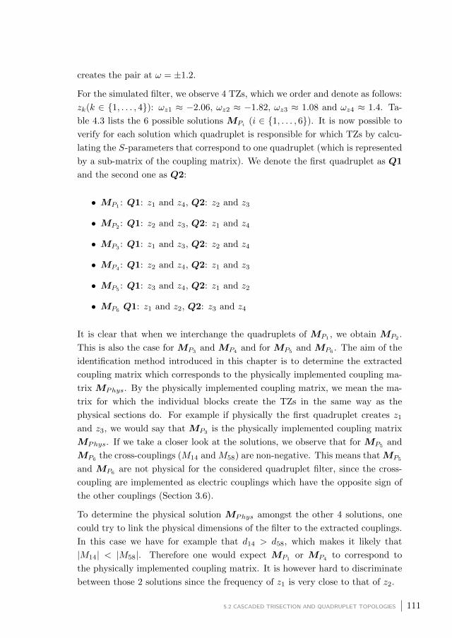
creates the pair at ω = ±1.2.

For the simulated filter, we observe 4 TZs, which we order and denote as follows:

zk(k ∈ 1, . . . , 4): ωz1 ≈ −2.06, ωz2 ≈ −1.82, ωz3 ≈ 1.08 and ωz4 ≈ 1.4. Ta-

ble 4.3 lists the 6 possible solutions MPi (i ∈ 1, . . . , 6). It is now possible to

verify for each solution which quadruplet is responsible for which TZs by calcu-

lating the S-parameters that correspond to one quadruplet (which is represented

by a sub-matrix of the coupling matrix). We denote the first quadruplet as Q1

and the second one as Q2:

• MP1: Q1: z1 and z4, Q2: z2 and z3




• MP5 : Q1: z3 and z4, Q2: z1 and z2

• MP6 Q1: z1 and z2, Q2: z3 and z4

It is clear that when we interchange the quadruplets of MP1, we obtain MP2

.

This is also the case for MP3and MP4

and for MP5and MP6

. The aim of the

identification method introduced in this chapter is to determine the extracted

coupling matrix which corresponds to the physically implemented coupling ma-

trix MPhys. By the physically implemented coupling matrix, we mean the ma-

trix for which the individual blocks create the TZs in the same way as the

physical sections do. For example if physically the first quadruplet creates z1

and z3, we would say that MP3is the physically implemented coupling matrix

MPhys. If we take a closer look at the solutions, we observe that for MP5and

MP6the cross-couplings (M14 and M58) are non-negative. This means thatMP5

and MP6 are not physical for the considered quadruplet filter, since the cross-

coupling are implemented as electric couplings which have the opposite sign of

the other couplings (Section 3.6).

To determine the physical solution MPhys amongst the other 4 solutions, one

could try to link the physical dimensions of the filter to the extracted couplings.

In this case we have for example that d14 > d58, which makes it likely that

|M14| < |M58|. Therefore one would expect MP1 or MP4 to correspond to

the physically implemented coupling matrix. It is however hard to discriminate

between those 2 solutions since the frequency of z1 is very close to that of z2.

5.2 CASCADED TRISECTION AND QUADRUPLET TOPOLOGIES 111

5.3 Identification of the Physically Implemented Coupling Matrix

This section explains the 2 phases of the identification method. The initialization

phase determines the physical coupling matrix for the initial design. The idea

behind the initialization is to first determine which of the sections (and thus

the blocks in the coupling matrix) are responsible for which TZs by adjusting

these sections separately. Once the physical matrix of the initial design M0Phys

is determined, the method tracks the physical solution(s) for the filter adjusted

during the tuning process by predicting the variations of the couplings. This

prediction is carried out using the design curves discussed in Chapter 3.

5.3.1 INITIALIZATION PHASE

The initialization phase heavily uses of the fact that one section only acts on a

specific set of TZs. This means that when we apply a variation to a physical

design parameter within a certain section, the TZs created by the other sections

remain unchanged. The blocks representing these sections must thus also remain

unchanged under this variation. By comparing the blocks (sub-matrices) linked

to the sections that should remain unchanged due to the applied variation in the

set of possible solutions, it is possible to determine MPhys.

Consider a filter consisting of 2 sections having nS solutions to the reconfigura-

tion problem. For the initial design values of the filter, the extraction procedure

yields nS possible coupling matrices. Next we apply a variation to a physical

parameter in the first section and we simulate the adapted structure. The ex-

traction procedure yields nS new coupling matrices. Since the variation only acts

on the first section, it only affects the TZs created by this section. Therefore the

block representing the second section should remain unchanged. The elements

of the block representing the second section are grouped in a new matrix (a

sub-matrix of the N ×N coupling matrix), which is denoted as Sxv . The index

x indicates the simulation (x ∈ 1, 2) and v indicates the index of the solution

(v ∈ 1, . . . , nS). We can now compare the matrices S1u and S2

v by calculating

the 2-norm of their difference:

δu,v =‖ S1u − S2

v ‖2 (5.3)

where (u, v ∈ 1, . . . , nS). Comparing all of the possible combinations requires

the calculation of n2S 2-norms. The combination (u, v) for which δu,v is mini-

mal corresponds to the pair of solutions for which the second blocks remained

maximally unaffected and thus to the pair of physically implemented coupling


matrices.

It is possible to generalize this rationale for cascaded coupling topologies having

p different sections. In the generalized version, we first apply physical variations

to all sections but the last. This simulation allows to determine the solutions for

which the last block remained unaffected. Next we apply physical variations in all

sections but the second last and last section. This simulation allows to determine

the solutions for which the last and second last block remained unaffected. We

repeat this action p− 1 times to determine the physically implemented coupling

matrix.

Initialization of the identification method for a CQ filter

We apply the initialization method to the initial design of the CQ filter discussed

in Section 5.2.1. We change the value of the distance between resonator 1 and 4

from d14 = 2.27 mm to d14 = 3 mm and simulate the new filter. Figure 5.2 shows

the effect of the parameter variation on |S21|. It is clear that the variation of

d14 only affects the position of z1 and z4. Next we calculate all of the 36 values

of δu,v. The minimal value is δ1,1 = 0.1192, which means that first solution

MP1 corresponds to MPhys. When the norms are sorted for increasing values,

the second value δ6,6 = 0.1543 is minimal. The maximal value is obtained for

δ3,4 = 2.1292.

0.85 0.9 0.95 1 1.05 1.1 1.15

−60

−40

−20

0

Frequency (GHz)

|S21|(

dB

)

Figure 5.2 |S21| for the initial dimension of the CQ filter (—) and after a variationof d14 = 2.27 mm → d14 = 3 mm (—).

5.3 IDENTIFICATION OF THE PHYSICALLY IMPLEMENTED COUPLING MATRIX 113

5.3.2 TRACKING PHASE

The drawback of the initialization phase is that it requires p − 1 extra EM-

simulations. We want however to minimize the number of EM-simulations re-

quired to tune the filter, since they represent the most-time consuming action

during the tuning procedure. Therefore we propose to use a different approach

once the initial M0Phys has been determined. The tuning of a filter is an iterative

process in which the physical dimensions are corrected at each iteration. In most

cases the initial dimensions have been determined using design curves relating

the couplings to one of the physical dimensions of the filter (Chapter 3). Al-

though these curves do not take into account the effects of all the dimensions on

the coupling parameters, they approximate the first order behavior of the inter-

resonator coupling as a function of the dominant design parameter well. These

curves thus allow to predict how the physical matrixMmPhys that will be found at

iteration m will vary in first order as a result of the corrected dimensions. Using

the design curves and the knowledge of the corrected dimensions, we calculate

a coupling matrix Mm+1Pred that predicts the values of the coupling for iteration

m + 1 starting from the values obtained in iteration m. Next we compare the

coupling matrices Mm+1Pi

(i ∈ 1, . . . , nS) extracted at iteration m + 1 to the

prediction matrix Mm+1Pred by calculating the 2-norm of the difference:

δm+1i =‖Mm+1

Pi−Mm+1

Pred ‖2 (5.4)

where i ∈ 1, . . . , nS. The solution Mm+1Pi

for which δm+1i is minimal is con-

sidered to correspond to Mm+1Phys.

The design curves extracted in Section 3.5 act as look-up tables where the cou-

pling for non-simulated values of the physical parameter are obtained by inter-

polation. To predict the effect of the variation of a geometrical parameter it is

convenient to have an analytic expression for these curves. Since the coupling

parameters behave smoothly in the region of interest and can be well approxi-

mated by quadratic polynomials [Amar 06], we estimate quadratic polynomials

in least-square senses from the data in the look-up table. Note that since we

only have curves for the inter-resonator couplings, we only take into account the

imaginary part of the inter-resonator coupling to calculate δni (5.4).

Tracking MmPhys for a CQ filter

Based on the comparison between the extracted matrix M0Phys and the target

coupling matrix, we adjust the dimensions of the initial filter. Figure 5.3 shows


|S11| and |S21| for the filter having adjusted dimensions. The dashed curves

show the response for the initial design. Figure 5.4 shows the curves (and the

least-square quadratic approximation) that are used to predict the effect of the

corrected dimensions. The prediction matrix M1Pred is:

0 0.8480 0 −0.1741 0 0 0 0

0.8480 0 0.7684 0 0 0 0 0

0 0.7684 0 0.6023 0 0 0 0

−0.1741 0 0.6023 0 0.6378 0 0 0

0 0 0 0.6378 0 0.5103 0 −0.3834

0 0 0 0 0.5103 0 0.8868 0

0 0 0 0 0 0.8868 0 0.7564

0 0 0 0 −0.3834 0 0.7564 0

(5.5)

Next we calculate the 6 differences between this prediction matrix and the phys-

ical solution for the initial design values M0Phys δ

1i (i ∈ 1, . . . , nS):

[δ11 . . . δ1

6

]=

[0.0144 0.1602 0.7724 0.7770 0.1819 0.2638

] (5.6)

It is clear that the first element δ11 is minimal and thus M1

P1= M1

Phys:

0.5506 0.8509 0 −0.1624 0 0 0 0.0025

0.8509 0.3164 0.7669 −0.0375 0 0 0 −0.0030

0 0.7669 0.4514 0.6016 0 0 0 0

−0.1624 −0.0375 0.6016 0.3927 0.6321 0 0 0.0006

0 0 0 0.6321 0.4082 0.5183 0.1024 −0.3894

0 0 0 0 0.5183 0.1157 0.8937 0

0 0 0 0 0 0.8937 0.4796 0.7664

0 0 0 0 −0.3894 0 0.7664 0.5136

(5.7)

Comparing the values of the matrix (5.5) to (5.7) shows that M1Pred predicts

the coupling parameters well. Moreover Table 5.1 shows that the corresponding

coupling matrix is closer to the target coupling matrix than M0Phys. Looking

5.3 IDENTIFICATION OF THE PHYSICALLY IMPLEMENTED COUPLING MATRIX 115

0.85 0.9 0.95 1 1.05 1.1 1.15

−60

−40

−20

0

Frequency (GHz)

|S11|&|S

21|(

dB

)

Figure 5.3 |S11| (—) and |S21| (—) for the adjusted filter. The dashed curves showthe S-parameters of the initial design.

1 1.2 1.4 1.6 1.8 21

2

3

4

5

6

7

·10−2

d (mm)

Cou

pli

ng

Figure 5.4 Desgin curves relating the inter-resonator coupling to the design parameterd: kE for the electric coupling (o) and its quadratic approximation (+).kM for the magnetic coupling (+) and its quadratic approximation (o).kB for the mixed coupling (+) and its quadratic approximation (o).

at Figure 5.3 shows that the bandwidth of the filter is closer to the desired

bandwidth, which also shows that the filter is closer to the golden goal. Note that

the lengths of the resonators have not been adjusted yet during this generation


which explains why the offsets have not changed that much.

Parameter Initial Iteration 1 TargetM12 0.9467 0.8509 0.8478M23 0.8549 0.7669 0.6896M34 0.6169 0.6016 0.5217M14 -0.2157 -0.1624 -0.1463M45 0.6656 0.6321 0.5328M56 0.5314 0.5183 0.4424M67 0.9410 0.8937 0.8218M78 0.8978 0.7664 0.7769M58 -0.3973 -0.3894 -0.3694M11 0.5780 0.5506 0M22 0.2656 0.3164 0M33 0.4738 0.4514 0M44 0.3833 0.3927 0M55 0.3863 0.4082 0M66 0.0267 0.1157 0M77 0.4558 0.4796 0M88 0.5494 0.5136 0

Table 5.1 Extracted and target coupling parameters for the initial design and theadjusted design after 1 iteration of the SOLR CQ filter.

5.4 Tuning of a CQ filter

We now use the identification method to tune the CQ filter introduced in Sec-

tion 4.8. The tuning is carried out ’manually’, meaning that the filter dimensions

are adjusted incrementally at each iteration based on a comparison between the

extracted and the target coupling matrix. Sometimes the adjustments are too

strong leading to an overshoot, sometimes they are too small leading to an

undershoot. The tuning procedure required 48 iterations to tune 19 physical

design parameters. The filter is implemented in a RT/duroid substrate with a

εr = 10.2 and a thickness of 1.27 mm. It is important to note that we have

first tuned the inter-resonator couplings and next we tuned the self-couplings.

During the tuning procedure, the filter is simulated for a realization with a

loss-less substrate and ideal conductors. The filter was simulated using ADS

Momentum [ADS 14] and 1 simulation takes around 8 min 30 s. The structure

was simulated for an infinite substrate and ground plane and with 60 mesh cells

per wavelength (of the shortest wavelength). Figure 5.5 shows the values for the

tuned design parameters in ADS. Figure 5.6 shows the layout of the filter in ADS

Momentum. Figure 5.7 shows |S11| and |S21| for the initial and final loss-less

5.4 TUNING OF A CQ FILTER 117

design together with the ideal response. The TZs are not exactly falling at the

correct golden goal positions due to the presence of the unavoidable parasitic

couplings.

Figure 5.5 Final design values for the tuned filter in ADS.

Figure 5.6 Layout of the filter in Momentum.

The final design is also simulated for the lossy substrate (tan δ = 0.0023). Fig-

ure 5.8 shows |S11| and |S21| for the final loss-less and lossy design together

with the ideal response. Inclusion of the substrate losses clearly degrades the

quality factors of the TZs and the insertion loss within the passband as could be


expected. Table 5.2 contains the extracted and ideal coupling parameters. The

extracted coupling parameters for the final design are very close to those of the

target coupling matrix: the maximum difference between the couplings is less

than 0.02 for the inter-resonator couplings. Note that there are still parasitic

couplings present and that the self-couplings of the resonators are not zero. For

the lossy filter, the real part of the diagonal elements is no longer negligible.

Table 5.4 contains the extracted quality factors of the resonators, the quality

factor of resonator k is determined as Qk = 1FBW Re(Mkk) (2.40). Note that

(2.40) only holds if the real parts of the non-diagonal couplings are zero.

If we take a closer look at Table 5.2, we observe that the parasitic coupling M13

and M57 are not negligible. To have an idea of their effect on the S-parameters,

we have added them to the ideal (target) coupling matrix and calculated the

corresponding S-parameters. Figure 5.9 shows that these couplings heavily de-

teriorate the reflection coefficient in the passband. Nevertheless the tuned filter

fulfills the specifications. It must be noted that some self-couplings (M33 and

M66) are relatively large for the tuned filter. This implies that these non-zero

self-couplings compensate somehow for the presence of M13 and M57. In the

next chapter we will use this effect to re-optimize the target coupling matrix,

changing the golden goal to take into account the parasitic couplings in the

physical filter.

Measurements

The final design is fabricated and measured for verification using a Vectorial

Network Analyzer. Figure 5.10 shows a picture of the fabricated filter. The

measurements show that there is a frequency offset and also that there is more

insertion loss than is predicted by the EM-simulator (Figure 5.11). The fre-

quency offset is due to an underestimate of the relative dielectric constant εr of

the substrate. In the simulation a dielectric constant of 10.2 was used where the

physical substrate has a εr of 10.6. This explains the shift of the center frequency.

The increase of the insertion loss is due to the presence of the conductor loss

of the copper which was not included in the simulation. To take into account

for these effects, the same structure was simulated using the updated substrate

and conductor parameters. To take into account the loss of the copper strip, the

conductivity was set to be 5.8 MSm . We have also included the effect of a finite

thickness of the metal strip, because this affects the coupling between the lines.

The thickness of the metal was set 17.5 µm. Figure 5.11 shows that the simula-

tions and measurement now agree quite well. Table 5.3 contains the extracted

coupling parameters of the measured and re-simulated filters. Note that these


Parameter Initial Final Loss-Less Final Lossy TargetMS1 0.9941 1.0452 1.0459 1.0416ML8 0.9920 1.0423 1.0431 1.0416M12 0.9467 0.8496 0.8493 0.8478M23 0.8549 0.6796 0.6812 0.6896M34 0.6169 0.5115 0.5120 0.5217M14 -0.2157 -0.1453 -0.1451 -0.1463M45 0.6656 0.5377 0.5385 0.5328M56 0.5314 0.4332 0.4317 0.4424M67 0.9410 0.8092 0.8089 0.8218M78 0.8978 0.7782 0.7775 0.7769M58 -0.3973 -0.3593 -0.3615 -0.3694M11 0.5780 -0.0115 -0.0093 0M22 0.2656 -0.0565 -0.0534 0M33 0.4738 0.1780 0.1662 0M44 0.3833 -0.0176 -0.0213 0M55 0.3863 -0.0070 -0.0073 0M66 0.0267 -0.1896 -0.2018 0M77 0.4558 0.0659 0.0715 0M88 0.5494 -0.0039 -0.0032 0M24 -0.0662 -0.1046 -0.0963 0M57 0.1388 0.0853 0.0907 0

Table 5.2 Extracted and target coupling parameters of the SOLR CQ filter.

are just estimation of the quality factors, since the real parts of the non-diagonal

couplings are not zero. The real parts of the non-diagonal couplings are 2 orders

of magnitude smaller than those of the diagonal elements. As expected the self-

couplings are still quite large, which is due to the frequency shift. Table 5.4

contains the extracted quality factors, which are much lower than in the case

where no metal loss was included as expected.


0.92 0.96 1 1.04 1.08−40

−30

−20

−10

0

Frequency (GHz)

|S11|(

dB

)

(a) |S11| for the initial design (—), the final loss-less design (—) and the idealresponse (- - -)

0.92 0.96 1 1.04 1.08

−60

−40

−20

0

Frequency (GHz)

|S21|(

dB

)

(b) |S21| for the initial design (—), the final loss-less design (—) and the idealresponse (- - -)

Figure 5.7 |S11| and |S21| for the initial design, the final loss-less design and the idealresponse


0.92 0.96 1 1.04 1.08−45

−35

−25

−15

−5

Frequency (GHz)

|S11|(

dB

)

(a) |S11| for the final lossy design (—), the final loss-less design (—) and the idealresponse (- - -)

0.92 0.96 1 1.04 1.08

−60

−40

−20

0

Frequency (GHz)

|S21|(

dB

)

(b) |S21| for the final lossy design (—), the final loss-less design (—) and the idealresponse (- - -)

Figure 5.8 |S11| and |S21| for the final lossy and loss-less design and the ideal response.


0.92 0.96 1 1.04 1.08−40

−30

−20

−10

0

Frequency (GHz)

|S11|(

dB

)

(a) |S11| for the ideal coupling matrix with extra couplings added (—), the finalloss-less design (—) and the ideal response (- - -)

0.92 0.96 1 1.04 1.08

−60

−40

−20

0

Frequency (GHz)

|S21|(

dB

)

(b) |S21| for the ideal coupling matrix with extra couplings added (—), the finalloss-less design (—) and the ideal response (- - -)

Figure 5.9 |S11| and |S21| for the ideal coupling matrix with extra couplings added,the final loss-less design and the ideal response


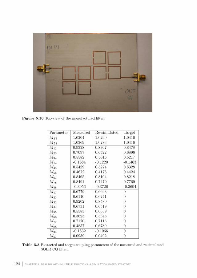
Figure 5.10 Top-view of the manufactured filter.

Parameter Measured Re-simulated TargetMS1 1.0204 1.0290 1.0416ML8 1.0369 1.0283 1.0416M12 0.9328 0.8307 0.8478M23 0.7097 0.6522 0.6896M34 0.5582 0.5016 0.5217M14 -0.1684 -0.1220 -0.1463M45 0.5429 0.5274 0.5328M56 0.4672 0.4176 0.4424M67 0.8465 0.8104 0.8218M78 0.8491 0.7470 0.7769M58 -0.3956 -0.3726 -0.3694M11 0.6779 0.6693 0M22 0.6110 0.6241 0M33 0.9202 0.8580 0M44 0.6731 0.6519 0M55 0.5583 0.6659 0M66 0.3623 0.5548 0M77 0.7170 0.7113 0M88 0.4857 0.6789 0M24 -0.1532 -0.1066 0M57 0.0939 0.0492 0

Table 5.3 Extracted and target coupling parameters of the measured and re-simulatedSOLR CQ filter.


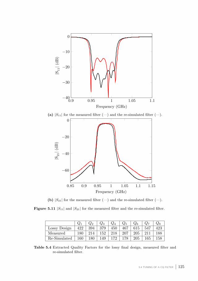
0.9 0.95 1 1.05 1.1−40

−30

−20

−10

0

Frequency (GHz)

|S11|(

dB

)

(a) |S11| for the measured filter (—) and the re-simulated filter (—).

0.85 0.9 0.95 1 1.05 1.1 1.15

−60

−40

−20

0

Frequency (GHz)

|S21|(

dB

)

(b) |S21| for the measured filter (—) and the re-simulated filter (—).

Figure 5.11 |S11| and |S21| for the measured filter and the re-simulated filter.

Q1 Q2 Q3 Q4 Q5 Q6 Q7 Q8

Lossy Design 422 394 379 450 467 615 547 423Measured 180 214 152 218 207 205 211 188Re-Simulated 160 180 149 172 178 205 165 158

Table 5.4 Extracted Quality Factors for the lossy final design, measured filter andre-simulated filter.


5.5 Conclusion

This chapter presents a novel method to identify the physically implemented

coupling matrix for CT and CQ filters. The example illustrates the utility of

the method during the tuning of cascaded topology filters. There are however

some limitations. Since the initialization phase is based on the specific relation

between the TZs and the quadruplets (or triplets), the method is limited to

this kind of topologies. When dealing with other topologies having multiple

solutions such as extended box topologies [Came 07a], the initialization procedure

must be adapted. Moreover when the number of sections grows, the number of

simulations to initialize the method grows as well which is disadvantageous when

the simulation time is high.

Once the M0Phys has been determined, the quadratic approximation of the de-

sign curves allows to predict the variations of the inter-resonator couplings with

sufficient accuracy. Note that we only track the inter-resonator coupling and

thus do not take into account the effect of parasitic couplings and self-couplings.

The quality of MPred thus heavily depends on the quality of the design curves

and the hypothesis that the inter-resonator couplings are mainly affected by the

distances between the resonators.

In order to avoid an exhaustive search among the possible solutions an alternative

approach could be to impose the target topology and use an optimization-based

method to extract the coupling parameters. A possible cost function in this case

is the distance between the imposed target matrix and the extracted coupling

parameters. To obtain an extracted coupling matrix at the beginning of the

tuning procedure a criterion must be assigned such that the extracted coupling

matrix has the same nature as the target matrix. If we consider for example

the case of two cascaded quadruplets, we can order the imaginary parts of the

extracted TZs in ascending order. As a criterion we can then assign the first

and last TZs to the first quadruplet and the second and third TZs to the sec-

ond quadruplet. Obviously this criterion must also hold for the target coupling

matrix. The benefits of such an approach are that we avoid the necessity of

multiple simulations and that the computations are faster. The main drawback

is that there is no guaranteed optimization convergence.

The tuning procedure used in Section 5.4 can be improved as well. In the

next chapter we present an automated tuning procedure which is based on the

Jacobian of the function that maps the coupling parameters to the physical

dimensions.


6Electromagnetic Optimization of Microstrip Bandpass Filters based on

Adjoint Sensitivity Analysis

This chapter introduces a novel computer-aided tuning (CAT) or optimization

method for coupled resonator microwave bandpass filters. The method is based

on the estimation of the Jacobian of the function that relates the geometrical

design parameters of the filter to the physically implemented coupling param-

eters. The Jacobian is estimated by combining the adjoint sensitivity of the

S-parameters with respect to the coupling parameters on the one hand and the

adjoint sensitivity of the S-parameters with respect to the physical filter design

parameters on the other hand.

Formal expressions exist to calculate the adjoint sensitivities of the S-parameters

with respect to the circuit parameters using the values of the extracted coupling

parameters only. Lately commercial EM-simulators, such as CST Microwave

Studio [CST 15], provide the adjoint sensitivities of the S-parameters with re-

spect to the geometrical or substrate parameters of the filter. One EM-simulation

therefore suffices to estimate the Jacobian. In the case of coupling topologies

with multiple solutions, the Jacobian is estimated for each solution separately.

This still requires only one EM-simulation. We present a criterion to determine

the physical solution using the estimated Jacobian matrices.

The tuning procedure first calculates the difference between the physically im-

plemented coupling matrix and the golden goal. Next it uses this difference

together with the Pseudo-inverse of the Jacobian, to obtain corrections for the

geometrical parameters. This process is repeated iteratively until the corrections

become sufficiently small with respect to a user specified goal. The CAT method

is applied to the design of a cascaded triplet (CT) and a single quadruplet (SQ)

microstrip filter.

127

6.1 Introduction

Over the last years various automated CAT methods have been developed to

optimize the physical dimensions (design parameters) of coupled resonator mi-

crowave bandpass filters. Some methods optimize a cost function based on the

values of S-parameters simulated at some well-chosen frequencies [Band 94b;

Arnd 04]. Other methods use a cost function based on the positions of the

poles and the zeros which are estimated starting from a rational model of the

S-parameters [Koza 02]. A third approach optimizes a cost function based on

the extracted coupling matrix [Lamp 04; Koza 06]. These methods share the

same time-consuming step which is the EM-simulation of the filter. Therefore

one of the main challenges is to reduce the number of EM-simulations needed to

tune the filter.

The coupling matrix based methods in [Lamp 04; Koza 06] correct the physical

dimensions using the Jacobian of the function that maps these parameters to the

extracted coupling parameters. The Jacobian matrix is estimated numerically

using forward differences. This estimation requires ng EM-simulations, where

ng is the number of physical design parameters of the filter. At each iteration

of the tuning method, the Jacobian is updated. The updates use the Broy-

den method [Broy 65] to reduce the required number of EM-simulations. The

methods discussed in [Lamp 04; Koza 06] all converge to a tuned design that

meets the specifications with a very low number of required EM-simulations.

Nevertheless the initial estimate still requires a high number of EM-simulation,

especially in the case of filters having a large number of design parameters.

Another shortcoming that is common to the current methods is that they do

not handle coupling topologies with multiple possible solutions.

The CAT method introduced in this chapter, estimates the Jacobian differ-

ently. It combines the adjoint sensitivity of the S-parameters with respect to

the coupling parameters on the one hand and the adjoint sensitivity of the S-

parameters with respect to the physical filter design parameters on the other

hand. Section 6.2 derives formal expressions to calculate the adjoint sensitivities

of the S-parameters with respect to the circuit parameters using the values of

the extracted coupling parameters only. Lately, commercial EM-simulators such

as CST Microwave Studio [CST 15] provide the adjoint sensitivities of the S-

parameters with respect to the geometrical or substrate parameters of the filter

without drastically increasing the simulation time. One EM-simulation therefore

suffices to estimate the Jacobian. Moreover, the Jacobian is re-estimated at each

iteration of the tuning procedure hereby improving the accuracy of the tuning.

128 CHAPTER 6 ELECTROMAGNETIC OPTIMIZATION OF MICROSTRIP BANDPASS FILTERS BASED ON ADJOINT

SENSITIVITY ANALYSIS

The method identifies the physically implemented coupling matrix whenever

non-canonical topologies are considered, again using only one EM-simulation.

One simulation suffices to estimate the Jacobian for each admissible solution.

Jacobian-based tuning the physical parameters requires one to determine their

Jacobian of the function relating the physical design parameters to the couplings

in the physical realization. The idea is that in a physical design, a coupling

parameter is mainly affected by a specific prior-known set of design parameters.

As a consequence the partial derivatives of the coupling parameter with respect

to these parameters are larger than the partial derivatives with respect to the

other design parameters having a second order effect at most. This assumption

allows one to predict which elements of the Jacobian are dominant in the case

that the underlying relation correspond to the physical relation. Selection of the

Jacobian of the physical relation boils down to finding the Jacobian for which

those elements are dominant. Note however that a single EM-simulation with the

determination of the Jacobian requires more time, since the adjoint sensitivities

are computed as well.

Section 6.6 explains the operation of the tuning method. Basically it calcu-

lates the corrections for the geometrical parameters using the difference between

the physically implemented coupling matrix and the target matrix and uses

the Pseudo-inverse [Ben 03] of the Jacobian to calculate the estimation of the

compensation to be applied. Thereto, the method minimizes the 2-norm of the

difference between the implemented and the target coupling parameters.

The physical dimensions are adjusted iteratively until the necessary corrections

become smaller than a user specified value. Section 6.7 applies the tuning

method to the design of a cascaded trisection filter. Section 6.8 applies the

tuning method to the design of a quadruplet filter. This design is more challeng-

ing due to the presence of parasitic couplings. The effect of the parasitics on the

response is much greater here as it is in the CT case. To take this into account

we re-optimize the target matrix (golden goal) during the tuning method as well.

Section 6.5 explains how this re-optimization of the target matrix is performed.

6.2 Adjoint Sensitivity of the S-parameters with respect to the CouplingParameters

In Section 2.6.2 we have derived equations to express the S-parameters as a

function of the inverse of the matrix A = jM +G+ jωIN+2. Here, the matrix

M contains the imaginary part of the extracted coupling matrix, the matrix G

contains the real part of the coupling matrix and the matrix IN+2 is an identity

6.2 ADJOINT SENSITIVITY OF THE S-PARAMETERS WITH RESPECT TO THE COUPLING PARAMETERS 129

matrix of size (N+2)×(N+2) whith the first and last elements on the diagonal

equal to 0. The S-parameters are obtained as follows:

S11 = 2[A−1]11 − 1

S12 = 2[A−1]1,N+2

S21 = 2[A−1]N+2,1

S22 = 2[A−1]N+2,N+2 − 1

(6.1)

where [A]kl denotes the element at position k, l of the matrix A. We now derive

a formal expression for∂Sij∂Mk,l

(ω). This represents the sensitivity of a scattering

parameter Sij with respect to a coupling parameter Mk,l taken at a certain

frequency ω. In Section 6.3 these sensitivities are used to estimate the Jacobian

of the functional relation between the physical filter parameters and the circuit

parameters. The sensitivities can be expressed as a function of A−1 . Remember

that the partial derivative of the inverse of a matrix A can be written as:

∂A−1

∂x= −A−1 ∂A

∂xA−1 (6.2)

Applying (6.2) to the expressions given in (6.1) yields:

For l 6= k :

∂S11

∂Mlk= −4j([A−1]1,l[A

−1]1,k)

∂S21

∂Mlk= −2j([A−1]N+2,l[A

−1]k,1 + [A−1]1,k[A−1]l,N+2)

∂S22

∂Mlk= −4j([A−1]N+2,l[A

−1]N+2,k)

For l = k :

∂S11

∂Mll= −2j[A−1]21,l

∂S21

∂Mll= −2j[A−1]1,l[A

−1]l,N+2

∂S22

∂Mll= −2j[A−1]2N+2,l

(6.3)



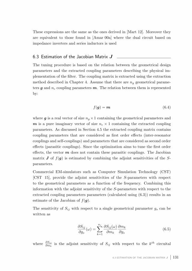
These expressions are the same as the ones derived in [Mart 12]. Moreover they

are equivalent to those found in [Amar 00a] where the dual circuit based on

impedance inverters and series inductors is used

6.3 Estimation of the Jacobian Matrix J

The tuning procedure is based on the relation between the geometrical design

parameters and the extracted coupling parameters describing the physical im-

plementation of the filter. The coupling matrix is extracted using the extraction

method described in Chapter 4. Assume that there are ng geometrical parame-

ters g and nc coupling parameters m. The relation between them is represented

by:

f(g) = m (6.4)

where g is a real vector of size ng×1 containing the geometrical parameters and

m is a pure imaginary vector of size nc × 1 containing the extracted coupling

parameters. As discussed in Section 4.5 the extracted coupling matrix contains

coupling parameters that are considered as first order effects (inter-resonator

couplings and self-couplings) and parameters that are considered as second order

effects (parasitic couplings). Since the optimization aims to tune the first order

effects, the vector m does not contain these parasitic couplings. The Jacobian

matrix J of f(g) is estimated by combining the adjoint sensitivities of the S-

parameters.

Commercial EM-simulators such as Computer Simulation Technology (CST)

[CST 15], provide the adjoint sensitivities of the S-parameters with respect

to the geometrical parameters as a function of the frequency. Combining this

information with the adjoint sensitivity of the S-parameters with respect to the

extracted coupling parameters parameters (calculated using (6.3)) results in an

estimate of the Jacobian of f(g).

The sensitivity of Sij with respect to a single geometrical parameter gs can be

written as

∂Sij∂gs

(ω) =

nc∑

k=1

∂Sij(ω)

∂mk

∂mk

∂gs(6.5)

where∂Sij∂mk

is the adjoint sensitivity of Sij with respect to the kth circuital

6.3 ESTIMATION OF THE JACOBIAN MATRIX J 131

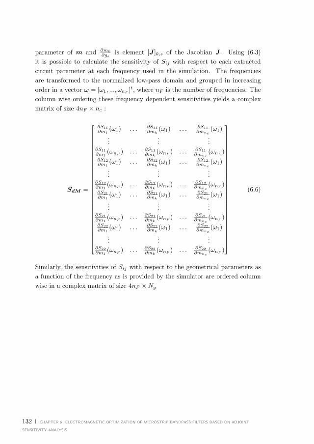
parameter of m and ∂mk∂gs

is element [J ]k,s of the Jacobian J . Using (6.3)

it is possible to calculate the sensitivity of Sij with respect to each extracted

circuit parameter at each frequency used in the simulation. The frequencies

are transformed to the normalized low-pass domain and grouped in increasing

order in a vector ω = [ω1, ..., ωnF ]t, where nF is the number of frequencies. The

column wise ordering these frequency dependent sensitivities yields a complex

matrix of size 4nF × nc :

SdM =

∂S11

∂m1(ω1) . . . ∂S11

∂mk(ω1) . . . ∂S11

∂mnc(ω1)

......

...∂S11

∂m1(ωnF ) . . . ∂S11

∂mk(ωnF ) . . . ∂S11

∂mnc(ωnF )

∂S12

∂m1(ω1) . . . ∂S12

∂mk(ω1) . . . ∂S12

∂mnc(ω1)

......

...∂S12

∂m1(ωnF ) . . . ∂S12

∂mk(ωnF ) . . . ∂S12

∂mnc(ωnF )

∂S21

∂m1(ω1) . . . ∂S21

∂mk(ω1) . . . ∂S21

∂mnc(ω1)

......

...∂S21

∂m1(ωnF ) . . . ∂S21

∂mk(ωnF ) . . . ∂S21

∂mnc(ωnF )

∂S22

∂m1(ω1) . . . ∂S22

∂mk(ω1) . . . ∂S22

∂mnc(ω1)

......

...∂S22

∂m1(ωnF ) . . . ∂S22

∂mk(ωnF ) . . . ∂S22

∂mnc(ωnF )

(6.6)

Similarly, the sensitivities of Sij with respect to the geometrical parameters as

a function of the frequency as is provided by the simulator are ordered column

wise in a complex matrix of size 4nF ×Ng



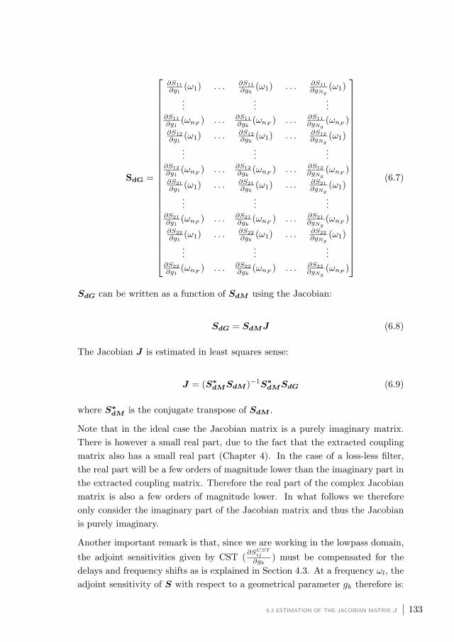
SdG =

∂S11

∂g1(ω1) . . . ∂S11

∂gk(ω1) . . . ∂S11

∂gNg(ω1)

......

...∂S11

∂g1(ωnF ) . . . ∂S11

∂gk(ωnF ) . . . ∂S11

∂gNg(ωnF )

∂S12

∂g1(ω1) . . . ∂S12

∂gk(ω1) . . . ∂S12

∂gNg(ω1)

......

...∂S12

∂g1(ωnF ) . . . ∂S12

∂gk(ωnF ) . . . ∂S12

∂gNg(ωnF )

∂S21

∂g1(ω1) . . . ∂S21

∂gk(ω1) . . . ∂S21

∂gNg(ω1)

......

...∂S21

∂g1(ωnF ) . . . ∂S21

∂gk(ωnF ) . . . ∂S21

∂gNg(ωnF )

∂S22

∂g1(ω1) . . . ∂S22

∂gk(ω1) . . . ∂S22

∂gNg(ω1)

......

...∂S22

∂g1(ωnF ) . . . ∂S22

∂gk(ωnF ) . . . ∂S22

∂gNg(ωnF )

(6.7)

SdG can be written as a function of SdM using the Jacobian:

SdG = SdMJ (6.8)

The Jacobian J is estimated in least squares sense:

J = (S∗dMSdM )−1S∗

dMSdG (6.9)

where S∗dM is the conjugate transpose of SdM .

Note that in the ideal case the Jacobian matrix is a purely imaginary matrix.

There is however a small real part, due to the fact that the extracted coupling

matrix also has a small real part (Chapter 4). In the case of a loss-less filter,

the real part will be a few orders of magnitude lower than the imaginary part in

the extracted coupling matrix. Therefore the real part of the complex Jacobian

matrix is also a few orders of magnitude lower. In what follows we therefore

only consider the imaginary part of the Jacobian matrix and thus the Jacobian

is purely imaginary.

Another important remark is that, since we are working in the lowpass domain,

the adjoint sensitivities given by CST (∂SCSTij

∂gk) must be compensated for the

delays and frequency shifts as is explained in Section 4.3. At a frequency ωl, the

adjoint sensitivity of S with respect to a geometrical parameter gk therefore is:

6.3 ESTIMATION OF THE JACOBIAN MATRIX J 133

[∂S11

∂gk(ωl)

∂S12

∂gk(ωl)

∂S21

∂gk(ωl)

∂S22

∂gk(ωl)

]=

[ej(ωlα11+β11) ∂S

CST11

∂gk(ωl) ej(ωl

α11+α222 +

beta11+β222 ) ∂S

CST12

∂gk(ωl)

ej(ωlα22+β22) ∂SCST22

∂gk(ωl) ej(ωl

α11+α222 +

beta11+β222 ) ∂S

CST21

∂gk(ωl)

] (6.10)

6.4 Determination of the Physically Implemented Coupling Matrix

In the case of coupling topologies supporting nS different possible solutions, the

extraction procedure yields nS different vectors mp (p ∈ 1, . . . , nS). This

means nS equivalent functions fp relate the design parameters g to the coupling

parameters mp. Among them only one function fPhys relates g to the physically

implemented coupling parameters mPhys.

To identify fPhys among all others, we assume that in a physical design a specific

coupling is mainly determined by a specific set of physical parameters and that it

is possible to determine which physical parameters influence the couplings most.

This assumption is also implicitly made during the initial dimensioning of the

filter. Remember that second order effects, such as loading of the resonators,

are also neglected there (Chapter 3). One can therefore predict which partial

derivatives ∂mk∂gs

are dominant for the physical design. These derivatives corre-

spond to the dominant elements of the Jacobian matrix JPhys of fPhys. Let V

denote the set of indexes corresponding to these elements. For each estimated

Jp, the relative influence of these predicted elements is calculated:

cp =

∑k,l∈V [Jp]

2l,k∑nc

m=1

∑ngn=1[Jp]2m,n

(6.11)

Here [Jp]l,k denotes the imaginary part of the element at position (l, k) of the

matrix Jp. In the set of equivalent Jacobian matrices one selects the matrix

for which cp is maximal. This matrix corresponds to the solution for which

the design parameters have the expected dominant main effects on the coupling

parameters. This solution can then safely be assumed to be the physical one. In

what follows we denote the physical function fPhys, the associated implemented

parameters mPhys and Jacobian JPhys as f , m and J respectively to make the

notation more readable.



6.5 Re-optimization of the Target Coupling Matrix

The presence of parasitic couplings can heavily deteriorate the performance of

the filter, even when the other inter-resonator and self-couplings correspond

to the requested target values. For the example discussed in Section 5.4, the

presence of the parasitic couplings M13 and M57 ruins the behavior of S11 in the

passband (Figure 5.9). It is however possible to compensate for this effect when

using the presence of non-zero diagonal elements. This can result in a final

filter, that meets the specification. In this section we propose to re-optimize

the target coupling matrix taking into account the presence of the observed

parasitic effects. We minimize the difference between reflection and transmission

coefficients created by the coupling matrix containing the parasitic elements and

the target values of reflection and transmission coefficients evaluated at a finite

number of frequencies.

We choose these frequencies in the passband for the reflection coefficient and

around the TZs for the transmission coefficient. We denote the target coupling

matrix with the observed coupling parameters added as Mpar,0 and the target

coupling matrix as Mid. We denote the response created by Mpar,0 as Spar,0kl

and the target response as Sidkl (k, l ∈ 1, 2). We now optimize the diagonal

elements of the matrixMpar,i to compensate the effect of the parasitic couplings.

The index i denotes the iteration and Spar,ikl is the response created by M tarpar,i.

The least squares cost function that is minimized is:

cpar,i =

√√√√nf11∑

f11=1

|Spar,i11 (ωf11)− Sid11(ωf11

)|2 +

nf21∑

f21=1

|Spar,i21 (ωf21)− Sid21(ωf21

)|2

(6.12)

where ωf11(f11 ∈ 1, . . . , nf11

) are the lowpass frequencies chosen in the pass-

band and ωf21 (f21 ∈ 1, . . . , nf21) are the lowpass frequencies chosen in the

vicinity of the TZs at finite frequencies. Similarly to Section 4.6 , the minimizer

of (6.12) is calculated using the Matlab function fminunc, which calculates the

minimum for an unconstrained multi-variable scalar function. Note that only

the diagonal elements of Mpar,i are varied during the optimization. We denote

the re-optimized target matrix as Mre

In the examples considered in this work, the inter-resonator couplings are mainly

affected by the distances between the resonators and the self-couplings by the

distances between the ends of the resonators. We assume that the parasitic cou-

6.5 RE-OPTIMIZATION OF THE TARGET COUPLING MATRIX 135

plings are mainly affected by the inter-resonator distances. In the case of strong

parasitic couplings, we first tune the filter until the inter-resonator distances

yield the target inter-resonator couplings. Next we re-optimize the target matrix

diagonal by taking into account the observed parasitic couplings by minimizing

cpar,i (6.12). We continue to tune the filters towards the newly found target

matrix Mre.

6.6 Tuning Method

6.6.1 CORRECTION OF THE DESIGN PARAMETERS

The optimization method calculates the update for the design parameters g such

that the corresponding circuital parameters f(g) = m coincide maximally with

the target coupling parameters m of the golden goal. Evaluating the function

f for the initial design parameters g0 yields the difference between the circuital

parameters of the initial design m0 and the target parameters m which allows

to evaluate the design error:

∆m0 = m− f(g0) (6.13)

The corrections of g0 necessary to improve the filter response are therefore read-

ily obtained as:

∆g0 = g1 − g0 = f−1(mo + ∆m0)− g0 (6.14)

where g1 are the design parameters of the improved filter. A linear approxima-

tion of f using the estimated Jacobian J0 evaluated at g0 yields:

m1 = f(g1) ≈ J0∆g0 +m0 (6.15)

Expression (6.15) approximates the correction of the design parameters using

the pseudo-inverse of the Jacobian J−10 :

∆g0 ≈ J−10 ∆m0 (6.16)

A simulation of the updated filter response yields the coupling parameters m1



and the Jacobian J1 in the same way as above. Repeating the process above then

allows to refine the correction until the necessary corrections become sufficiently

small:

‖ ∆gk ‖∞= maxl

[∆gk]l < δcorr (6.17)

where δcorr is a user-defined value. Since there is no point in calculating geo-

metrical parameters more precisely than the limits imposed by the fabrication

tolerance, a valid choice for δcorr is readily found to be the accuracy of the fabri-

cation process. For all considered examples, the optimization method converges

after a number of iterations smaller than the number of design parameters to be

tuned.

When the parasitic couplings heavily influence the response, we tune the filter

until the corrections for the inter-resonator distances become smaller than δcorr.

To this end, we order the inter-resonator couplings in a vector gdk. Next we re-

optimize the target coupling matrix as discussed in Section 6.5 and order them

into a vector mre.

6.6.2 OPTIMIZATION ALGORITHM

1. Approximation of a frequency template to obtain the ideal rational scat-

tering matrix that fulfills the specifications (Chapter 2)

2. Synthesis of the target coupling matrix M (the couplings are ordered in a

vector m). In the case of multiple solutions, one solution is chosen as the

target matrix

3. Computation of the initial design parameters gk of the filters’ physical

implementation, where k = 0 (Chapter 3)

4. Full-wave EM-simulation of the filters S-parameters in the frequency band

of interest and the adjoint sensitivities of the S-parameters with respect

to the design parameters gk

5. Extraction of the coupling parameters (Chapter 4):

(a) Rational approximation of the simulated S-parameters.

(b) Coupling matrix synthesis

(c) Determination of all the possible solutions corresponding to the im-

plemented coupling topology

6.6 TUNING METHOD 137

6. Estimation of the Jacobian of the couplings with respect to the physical

parameters for each solution and determination of the physically imple-

mented coupling matrix using expression (6.11) (Section 6.3)

7. Computation of the error of the circuit parameters ∆mk (Section 6.6.1)

8. Estimation of the correction for the design parameters ∆gk ≈ J−1k ∆mk

9. Case of strong parasitics: re-optimize the target to obtain mre if

‖ ∆gdk ‖∞< δcorr

10. Termination of the optimization process if ‖ ∆gk ‖∞< δcorr

11. Update of the design parameters: gk+1 = gk + ∆gk and return to step 4

6.7 Tuning of a CT filter

In this section the tuning method is applied to the design of a 6th order CT

filter. The filter is designed to have center frequency fc = 1.2 GHz, a fractional

bandwidth FBW = 0.04, a minimum return loss RL of 22 dB and 2 finite

transmission zeros (TZs) at ω = 1.15 and ω = 2.1. The target coupling matrix is

synthesized using Dededale-HF [Seyf 00]. There are 2 solutions to the reduction

problem of which one is chosen (arbitrarily). The chosen target coupling matrix

is:

0 1.0422 0 0 0 0 0 0

1.0422 0.0394 0.8355 0.2745 0 0 0 0

0 0.8355 −0.3377 0.5789 0 0 0 0

0 0.2745 0.5789 0.1138 −0.5986 0 0 0

0 0 0 −0.5986 0.1349 0.3544 0.6483 0

0 0 0 0 0.3544 −0.8252 0.5942 0

0 0 0 0 0.6483 0.5942 0.0394 1.0422

0 0 0 0 0 0 1.0422 0

(6.18)

In the chosen solution, the first triplet realizes the TZ at ω1 = 2.1 and the second

one the TZ at ω2 = 1.15

The filter is implemented on a RO4360 substrate with a thickness of 1.016 mm

and εr = 6.15. To implement the λ2 -resonators we use a variation of the SOLR

resonator, which is not square but rectangular. Figure 6.1 shows the top-view



Figure 6.1 Top-view of the layout of a sixth order cascaded triplet filter.

of the layout of the CT filter. Table 6.1 contains the initial dimensions of the

filter. There are 15 design parameters which are the spacing dkl between the

resonators k and l and the distance between the ends gi of the resonator i. Note

that the positions of the feeding lines ti are also design parameters. They are

however not included in the optimization method, since CST is not capable to

calculate the adjoint sensitivity with respect to a parameter that influences the

position of a port. Therefore these parameters have to be tuned manually.

Figure 6.2 shows the S-parameters of the initial design. Note that the initial

design is far away from the target design. We did not use design curves to

obtain initial values for the mixed couplings M12, M23, M45 and M56 but we

have chosen values within the range of values found for the other spacings using

visual inspection.

The coupling matrices are extracted using the method described in Chapter 4.

There are 2 solutions to the reconfiguration problem and thus there are 2 possible

Jacobian matrices too. The parameters are ordered such that dominant elements

should be positioned on the main diagonal of the matrix. When we calculate

the relative influence of these dominant elements over the others for the first

iteration, we find the following values for cp as defined in (6.11):

cp =[0.9104 0.2024

](6.19)

6.7 TUNING OF A CT FILTER 139

Physical parameter Initial Value (mm) Final Value (mm)a 16.7 16.7b 16.5 16.5w 1 1t1 4.6 4.6t2 4.6 4.6d12 0.6 0.74d23 1.4 1.16d13 2.1 1.9d34 2.2 2.74d45 1.5 1.71d56 1.4 1.05d46 1.3 1.37g1 0.75 0.61g2 1.1 0.8g3 0.65 0.47g4 0.6 0.48g5 1.3 1.22g6 0.75 0.55

Table 6.1 Initial and final values for the physical design parameters of the CT filter.

This indicates that the first solution corresponds to the physically implemented

coupling matrix. Table 6.2 contains the coupling parameters associated to the

initial design parameters.

Figure 6.3a compares the magnitude of the adjoint sensitivity ∂S11

∂M12(ω) obtained

using (6.3) to ∂S11

∂d12(ω) obtained using CST. Similarly, Figure 6.3b compares

the magnitude of the ∂S21

∂M12(ω) to ∂S21

∂d12(ω). We observe that the trend of the

sensitivity as a function of ω is very similar. This indicates that the S-parameters

vary similarly to a change of d12 and M12. There is however a difference since the

other geometrical parameters also act on M12. Figure 6.4 compares the adjoint

sensitivity of S11 with respect to d12 and M12 respectively in the complex plane.

Besides the difference in amplitude, we also observe a phase shift of −π rad.

This phase shift is due to the fact that in (6.3) the S-parameters are derived

with respect to Mkl instead of jMkl. If we compensate for this by multiplying∂Smn∂Mlk

by −j, we observe a similar phase behavior for both adjoint sensitivities.



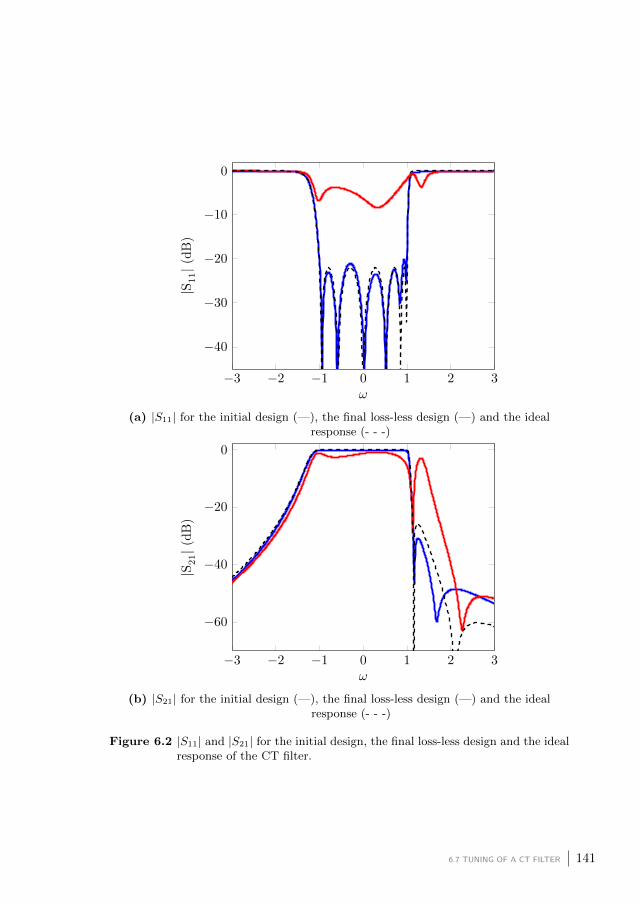
−3 −2 −1 0 1 2 3

−40

−30

−20

−10

0

ω

|S11|(

dB

)

(a) |S11| for the initial design (—), the final loss-less design (—) and the idealresponse (- - -)

−3 −2 −1 0 1 2 3

−60

−40

−20

0

ω

|S21|(

dB

)

(b) |S21| for the initial design (—), the final loss-less design (—) and the idealresponse (- - -)

Figure 6.2 |S11| and |S21| for the initial design, the final loss-less design and the idealresponse of the CT filter.


The elements of m and g are ordered such that the first row of the Jacobian

corresponds to the partial derivatives ∂M21

∂gs, s ∈ 1, . . . , 13, where gs is one of

the 13 geometrical design parameters. The first 7 elements of this row correspond

to the partial derivatives with respect to the spacing between the resonators:

[∂M21

∂d12

∂M21

∂d23

∂M21

∂d13

∂M21

∂d34

∂M21

∂d45

∂M21

∂d56

∂M21

∂d46

]=

[−0.7061 −0.0086 −0.1677 0.0529 −0.0050 −0.0121 0.0012

] (6.20)

It is clear that M12 mainly depends on d12 as expected. The negative sign of∂M21

∂d12also corresponds to what we physically expect: if the distance increases,

the coupling decreases and vice versa. The other parameter that mainly influ-

ences M12 is d13. This is logical since, d13 determines the offset of resonator 1

with respect to resonator 2. As expected M12 is mainly determined by design

parameters in the first triplet. The 6 last elements of this row in the Jacobian

correspond to the partial derivatives with respect to the spacing between the

ends of each resonator:

[∂M21

∂g1

∂M21

∂g2

∂M21

∂g3

∂M21

∂g4

∂M21

∂g5

∂M21

∂d56

]=

[0.0912 −0.0503 0.0058 −0.0191 0.0058 0.0012

] (6.21)

It is clear that M12 is mainly influenced by g1 and g2, which is consistent with

what we expect.

The value of δcorr was set to 0.01 mm and after 4 iterations (5 EM-simulations)

we found a ‖ ∆gk ‖∞= 0.01. On average, an EM-simulation takes 2 hours 30 min

(with adjoint sensitivities included). Note that the adaptive meshing is included

in this time and this already takes 1 hour. An EM-simulation without adjoint

sensitivities takes 2 hours 10 min on average, indicating that the extra time

that is needed to calculate the adjoint sensitivities is acceptable. Figure 6.5

shows the evolution of the inter-resonator couplings and of the self-coupling

during the tuning process. The figure shows that after 2 iterations, the coupling

parameters are already very close to the target values. The last 2 iterations

can be seen as fine tuning. Note that for clarity of the figure, we have not

taken into account the sign of the inter-resonator couplings. Figure 6.6a shows

the evolution of the 2-norm and the ∞-norm of the design error ∆m. Note



−2 −1 0 1 2−10

0

10

20

ω

dS

11/d

g12

and

dS

11/d

M12

(dB

)

(a) Comparison between the adjoint sensitivities | ∂S11∂M12

| (—) and | ∂S11∂d12| (- - -).

−2 −1 0 1 2

−40

−20

0

ω

dS

21/d

g12

and

dS

11/d

M12

(dB

)

(b) Comparison between the adjoint sensitivities | ∂S21∂M12

| (—) and | ∂S21∂d12| (- - -).

Figure 6.3 Comparison between the adjoint sensitivities of the S-parameters withrespect to the geometrical (- - -) and circuit or coupling parameters (—).

that ∞-norm is the smallest after iteration 2 (at simulation 3), meaning that

the maximum difference with respect to the target value is the lowest at that

iteration. However the 2-norm of the vector ∆m is clearly minimal after the

4th iteration. Figure 6.6b shows the evolution of the 2-norm and the ∞-norm of

the correction vector ∆g during the tuning process. The maximum correction

proposed for the second iteration is larger than for the first, for the following


−6 −4 −2 0 2

−5

0

5

Real part of adjoint sensitivity

Imag

inar

yp

art

ofad

join

tse

nsi

tivit

y

Figure 6.4 Comparison between the adjoint sensitivities ∂S11∂M12

(—), −j ∂S11∂M12

(—) and∂S11∂d12

(- - -).

iteration it clearly decreases. Note that these corrections are in mm. Finally

remark that the TZs do not perfectly coincide. This is due to the presence

of the unwanted parasitic couplings M16,M26 and M36 (shown in Table 6.2).

We have not re-distributed the parasitic couplings, so note that they are not

necessarily physically located at those positions. Figure 6.7 shows the response

that is obtained from the ideal coupling matrix when the parasitic couplings

are added. It is clear that then the TZs now coincide. Note however that the

parasitic couplings are small, we therefore choose not to re-optimize the target

matrix.



Parameter Initial Final TargetMS1 1.0605 1.0485 1.0422ML8 1.0490 1.0407 1.0422M12 0.9199 0.8342 0.8355M23 0.4751 0.5800 0.5789M13 0.2146 0.2768 0.2745M34 -0.1227 -0.5993 -0.5986M45 0.4434 0.3552 0.3544M56 0.4594 0.5944 0.5942M46 0.7212 0.6449 0.6483M11 -0.0758 0.0385 0.0394M22 -0.7571 -0.3351 -0.3377M33 -0.1227 0.1066 0.1138M44 -0.0357 0.1411 0.1349M55 -0.8558 -0.8155 -0.8252M66 -0.3068 0.0349 0.0394MSL 0 -0.0001 0MS6 0 -0.0001 0ML1 0 -0.0001 0M16 -0.0010 -0.0007 0M26 0.0155 0.0133 0M36 0.0036 0.0044 0

Table 6.2 Extracted and target coupling parameters of the SOLR CT filter.


1 2 3 4 5

0.2

0.4

0.6

0.8

1

EM-simulation

Mkl

(a) Evolution of the inter-resonator couplings during the tuning process.

1 2 3 4 5−1

−0.5

0

EM-simulation

Mkk

(b) Evolution of the self-couplings during the tuning process.

Figure 6.5 Evolution of the coupling parameters during the tuning process. The fulllines mark the target values of the first triplet and the dashed lines markthe target values of the second triplet.



1 2 3 4 5

0

0.2

0.4

0.6

0.8

EM-simulation

||∆m|| 2

and

max(∆

m)

(a) The 2-norm of the error vector ‖ ∆m ‖2 (-o) and the maximal error ‖ ∆m ‖∞(-x).

1 2 3 4 50

0.2

0.4

0.6

0.8

EM-simulation

||∆g|| 2

and

max(∆

g)

(b) The 2-norm of the correction vector ‖ ∆g ‖2 (-o) and the maximal correction‖ ∆g ‖∞ (-x) (mm).

Figure 6.6 Evolution of the 2-norm and ∞-norm of the error vector ∆m and thecorrection vector ∆g.


−3 −2 −1 0 1 2 3

−60

−40

−20

0

ω

|S21|(

dB

)

Figure 6.7 |S21| (dB) of the final (—) design and response obtained from the idealcoupling matrix (- - -) when the parasitic couplings are added versus theideal response (- - -).



6.8 Tuning of a SQ filter

In this section the tuning method is applied to the design of a SQ filter. In

this type of filter the parasitics affects the response more than in the case of

the CT filter. Therefore we will re-optimize the target matrix during the tuning

procedure. The filter is designed to have center frequency fc = 1.2 GHz, a

fractional bandwidth FBW = 0.04, a return loss of 22 dB and 1 symmetric

TZ pair at ω = ±1.5. The filter is implemented on a RO4360 substrate with a

thickness of 1.016 mm and εr = 6.15. To implement the λ2 -resonators we use

SOLR structures. The filter has the same lay-out as the example discussed in

Section 3.6 (Figure 3.14). The target coupling matrix is given in Table 6.3. The

initial values for the filter are generated using the design curves (Section 3.6)

and are given in Table 6.4.

Parameter Initial Iteration 1 TargetMS1 1.0654 1.0702 1.0580ML4 1.0651 1.0337 1.0580M12 0.8683 0.8352 0.8365M23 0.9111 0.8766 0.8713M34 0.8522 0.8393 0.8365M14 -0.4301 -0.4058 -0.4089M11 0.1731 0.0033 0M22 0.2837 -0.0177 0M33 -0.0708 0.0232 0M44 0.1733 -0.0092 0MSL 0.0081 0.0076 0MS4 0.0118 0.0113 0ML1 0.0118 0.0113 0M24 0.1665 0.1471 0

Table 6.3 Extracted and target coupling parameters of the SOLR SQ filter.

6.8.1 TUNING TO THE ORIGINAL TARGET MATRIX

In the first part of the tuning procedure, we tune the filter such that all of

the coupling parameters are as close as possible to the target coupling matrix.

Similarly as for the CT filter, we set the value of the minimal correction δcorr to

0.01 mm. After one iteration, all of the inter-resonator couplings are very close

to the target values (maximal difference is -0.0053) and ‖ ∆gdk ‖∞= −0.0067

mm. Moreover the values of the diagonal elements are also very close to target

values (maximal difference is 0.0232). Table 6.3 shows however that the para-

sitic coupling M34 has the same order of magnitude as the other inter-resonator

6.8 TUNING OF A SQ FILTER 149

Physical parameter Initial Value (mm) Iteration 1 (mm)a 16.7 16.7w 1 1t1 5 5t2 5 5d12 1.6 1.64d23 2 2.13d34 1.6 1.65d14 1.7 1.75g1 1.5 1.68g2 1.5 1.83g3 1.5 1.44g4 1.5 1.69

Table 6.4 Initial and final values for the physical design parameters of the SQ filter.

couplings present in the filter. Figure 6.8 shows |S11| and |S21| for the ideal

response, the initial values and for the first iteration. One would say that the

adjustments of the filter deteriorated the response of the filter. Note however

that we have only tuned for the couplings present in the target coupling matrix,

without taking into account the parasitic coupling M24. If we add the observed

value of M24 to the ideal target matrix and look at the corresponding result, we

observe that the response is very close to the observed response after iteration 1.

There is however still an offset since the diagonal elements M22 and M33 are not

sufficiently close to 0. Therefore it has no use to further tune towards the initial

target coupling matrix that does not take into account the parasitic couplings.

We thus re-optimize the target coupling matrix, taking into account the value

of M24 at iteration 1.

6.8.2 RE-OPTIMIZATION OF THE TARGET COUPLING MATRIX

The target coupling matrix is re-optimized using the method discussed in Sec-

tion 6.5. This means that we only re-optimize the diagonal values of the target

coupling matrix. The values of the re-optimized target matrix are given in Ta-

ble 6.5. Figure 6.9 shows the response of iteration 2 and the re-optimized ideal

response. The filter is now much closer to the ideal response as was the case

both for the initial design and after iteration 1. Table 6.5 compares the extracted

coupling parameters for iteration 2 to the re-optimized coupling parameters. The

table shows that the implemented coupling parameters are very close to the re-

optimized target values: the maximal difference is -0.0106. Figure 6.9 shows

however that the implemented response does not match the re-optimized re-



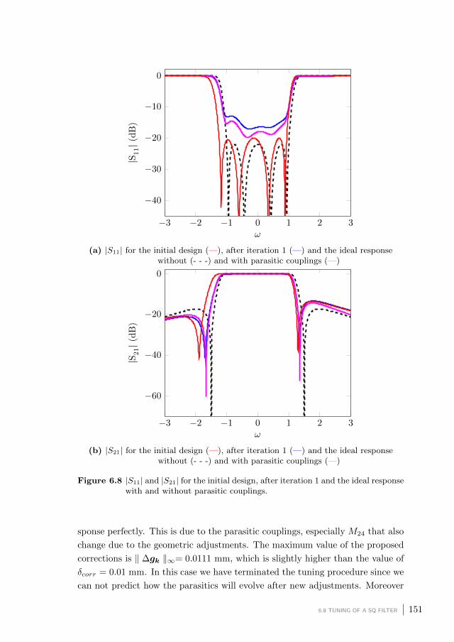
−3 −2 −1 0 1 2 3

−40

−30

−20

−10

0

ω

|S11|(

dB

)

(a) |S11| for the initial design (—), after iteration 1 (—) and the ideal responsewithout (- - -) and with parasitic couplings (—)

−3 −2 −1 0 1 2 3

−60

−40

−20

0

ω

|S21|(

dB

)

(b) |S21| for the initial design (—), after iteration 1 (—) and the ideal responsewithout (- - -) and with parasitic couplings (—)

Figure 6.8 |S11| and |S21| for the initial design, after iteration 1 and the ideal responsewith and without parasitic couplings.

sponse perfectly. This is due to the parasitic couplings, especially M24 that also

change due to the geometric adjustments. The maximum value of the proposed

corrections is ‖ ∆gk ‖∞= 0.0111 mm, which is slightly higher than the value of

δcorr = 0.01 mm. In this case we have terminated the tuning procedure since we

can not predict how the parasitics will evolve after new adjustments. Moreover

6.8 TUNING OF A SQ FILTER 151

we are very close to the target values. Finally note that S21 of the re-optimized

response attenuates less in the upper stopband when compared to the original

ideal response.

Parameter Iteration 2 Re-optimized Target TargetMS1 1.0703 1.0580 1.0580ML4 1.0725 1.0337 1.0580M12 0.8329 0.8365 0.8365M23 0.8687 0.8713 0.8713M34 0.8338 0.8365 0.8365M14 -0.4107 -0.4089 -0.4089M11 -0.0090 -0.0069 0M22 0.0501 0.0396 0M33 -0.2169 -0.2119 0M44 -0.0521 -0.0491 0MSL 0.0077 0.0076 0MS4 0.0114 0.0113 0ML1 0.0114 0.0113 0M24 0.1514 0.1471 0

Table 6.5 The extracted coupling parameters for iteration 2, the original target andthe re-optimized target matrix.



−3 −2 −1 0 1 2 3

−40

−30

−20

−10

0

ω

|S11|(

dB

)

(a) |S11| for iteration 2 (—), the ideal response (- - -) and the target re-optimized forthe parasitic couplings (—).

−3 −2 −1 0 1 2 3

−60

−40

−20

0

ω

|S21|(

dB

)

(b) |S21| for iteration 2 (—), the ideal response (- - -) and the target re-optimized forthe parasitic couplings (—).

Figure 6.9 |S11| and |S21| iteration 2, the ideal response and the target re-optimizedfor the parasitic couplings.

6.9 Discussion

The major benefit of using a coupling matrix based cost function is that in the

vicinity of the solution the Jacobian matrix of the function relating the design

parameters to the coupling parameters is almost diagonal. This makes that

a certain coupling parameter mainly depends of one design parameter and is

6.9 DISCUSSION 153

practically independent of the other design parameters. Moreover it is known

that coupling parameter behaves more or less quadratic as a function of the

design parameters [Amar 06]. Therefore the tuning algorithm requires only a few

iterations. Moreover there are no local minima in the region where the extracted

coupling matrix models the filter behavior well. This is a major advantage

with respect to other tuning methods based on pole-zero matching [Koza 02],

which optimize a cost function based on the position of the poles and the zeros.

The relation between the poles and zeros and the design parameters is more

complex than the relation between physically implemented couplings and the

design parameters. Thus there is no guarantee that there are no local minima

in the vicinity of the solution.

6.10 Remarks

The first remark is related to the implementation of the tuning procedure in

Matlab. Due to a bug in CST [CST 15], it was necessary to divide the adjoint

sensitivity of the S-parameters with respect to the geometrical parameters (pro-

vided by CST) by 2. CST has guaranteed that in the future version this error

will be resolved. We must remark that in the case the Fast reduced order model

simulation setting is used, the adjoint sensitivities are correct.

The second remark has to do with the simulation time. At the moment it is

rather high. This is mainly due to the adaptive meshing which takes almost half

of the simulation time. We plan to investigate how we can decrease the required

simulation time without loosing accuracy.

As a final remark, we point out that at the moment the method can not be used

to tune the input-to-first-resonator and output-to-N th-resonator coupling. The

reason for that is that it is not possible to obtain the adjoint sensitivity with

respect to parameters that touch the ports.

6.11 Conclusion

This chapter presents a novel CAT method based on the estimation of the Ja-

cobian matrix relating the physical design parameters to the physically imple-

mented coupling matrix. The main novelty of the method is the estimation of

the Jacobian matrix of the coupling parameters with respect to the physical

design parameters using adjoint sensitivities. To estimate the Jacobian one

EM-simulation suffices. This is a vast improvement over the finite difference

evaluation where an extra EM-simulation is needed for each physical design



parameter. Note that an EM-simulation with adjoint sensitivities requires more

time than a simulation without. Nevertheless this does not drastically increase

the simulation time. Another benefit of the Jacobian estimation method is that

it offers a criterion to determine the physically implemented coupling matrix in

the case of non-canonical topologies. The novel CAT method is used to tune a

6th order CT and 4th order SQ filter. Both examples shows that knowledge of the

Jacobian matrix drastically decreases the number of EM-simulations required to

tune the filter. For the CT filter 4 iterations (5 EM-simulation) suffice, where the

filter has 13 design parameters. Note that an estimation of the Jacobian using

finite differences would already take 13 extra EM-simulations. In the example of

SQ filter, the target coupling matrix had to be re-optimized due to the presence

of strong parasitic couplings. Nevertheless the tuning only required 2 itera-

tions (3 EM-simulations). Note that the proposed strategy to handle parasitic

couplings must be further improved in the future, since it does not take into

account the fact that parasitic couplings also change due to adjustments of the

physical parameters. We may conclude that this method is an ideal candidate

for EM-based fine-tuning of coupled resonator bandpass filters.

6.11 CONCLUSION 155

PART II

Metamodel Approach

157

7Efficient and Automated Generation of Multidimensional Design Curves

using Metamodels

This chapter introduces a method to automatically generate multidimensional

design curves for the initial dimensioning of coupled-resonator filters. As we have

seen in Chapter 3, these curves are look-up tables that relate the inter-resonator

couplings and the input and output couplings (or external quality factors) to the

physical design parameters of the filters. To minimize the number of EM simula-

tions required for the generation of the curves, these curves often consider only a

single design parameter. In reality, several design parameters simultaneously in-

fluence the inter-resonator coupling and external quality factors. In this chapter,

a metamodeling method is used to generate multidimensional design curves with

a reasonable number of EM simulations, while maintaining a good accuracy. The

generation process only requires one to provide ranges of the design parameters

over which the curves are generated. This information is readily available based

on geometric and process related arguments. The remainder of the generation

process requires no further user interaction. To show the applicability of the

method, we generate design curves for the design of a coupled hairpin resonator

filter. We use the extracted curves to generate initial values for a 5th order filter

for 3 different design scenarios.

7.1 Introduction

In Chapter 3 a method to generate initial values for coupled-resonator bandpass

filters was introduced. The method first divides the filter into building blocks.

Next, it dimensions these blocks separately and finally merges them together.

The dimensioning of each individual block relies on design curves to relate the

physical parameters to the coupling parameters [Pugl 00; Pugl 01]. The classical

generation procedure of design curves (discussed in Section 3.5), first computes

the frequency response function (FRF) of a building block (section of coupled

159

resonators or single input/output resonator) at a discrete set of frequency sam-

ples for some ”well-chosen” values of a design parameter. For each value of the

design parameter, the corresponding coupling parameter and external quality

factor are extracted from the FRFs (the frequency-domain scattering parame-

ters). This process yields sampled design curves (or look-up tables) on some kind

of regular grid in the geometric parameters. As the FRFs are usually obtained

using electromagnetic (EM) field solvers [Swan 07b], the design curve generation

procedure often becomes very time-consuming.

To our knowledge, no real guidelines/techniques exist to determine the set of

frequencies and the values of the design parameters the EM simulations that

have to be selected to obtain design curves with a minimal number of the EM

simulations and frequencies while the desired accuracy is preserved. Preferably,

multiple design parameters should be considered in the design curves generation

process. As a consequence, the number of EM simulations and therefore the

design curves generation time grow very rapidly if some kind of regular grid is

chosen for the geometrical parameters, even though many grid points bring only

a limited amount of information.

Here, we propose an efficient and automated metamodel-based design curves

generation procedure. It overcomes the limitations of the classical design curve

generation procedure. A metamodel [Klei 08] is a very efficient representation

of a multi-dimensional function that provides a functional relationship between

input and output variables. In our case, these correspond to physical design pa-

rameters and the coupling parameters and external quality factors, respectively.

Metamodels can have different basis functions: e.g. polynomial functions, radial

basis functions, or splines [Klei 08]. Adaptive sampling methods [Wang 07] limit

the amount of computationally expensive numerical simulations needed for the

generation of metamodels while maintaining the coverage of the input space.

This chapter presents a metamodeling approach that automates and drastically

speeds-up the generation of multidimensional design curves for microwave filters.

The coupling parameter and the external quality factors of coupled-resonator

filters are modeled as a function of multiple geometrical design parameter. To

obtain it, a system identification approach is combined with an adaptive fre-

quency sampling. This allows to efficiently and accurately extract the values

of the coupling parameter and external quality factors over the complete de-

sign space using a set of design parameter values automatically chosen by the

metamodeling adaptive sampling and starting from frequency-domain scattering

parameters. The values of the coupling parameters extracted from the simulated

160 CHAPTER 7 EFFICIENT AND AUTOMATED GENERATION OF MULTIDIMENSIONAL DESIGN CURVES USING

METAMODELS

data are used for the generation of the metamodels. The user interaction is

limited to providing the frequency range of interest, the design parameters of

interest and their corresponding ranges. If the design parameters ranges are

chosen wide enough to allow the modeling of all physically significant variations

of the coupling parameter and external quality factor, then the design curves can

be used for multiple design cases. Multidimensional design curves that depend

on multiple design parameters can be generated in a reduced amount of time.

This offers a significant flexibility to the designer while generating initial values

for the filter design. The proposed metamodeling method is validated by the

generation of the design curves of a coupled hairpin resonator filter. These

curves are then used for multiple initial designs.

7.2 Generation of the Design Curves using Metamodels

This section describes the generation of metamodels linking the coupling param-

eters and the external quality factors to the geometrical parameters of the filter.

In Section 3.5.1 we have seen how to extract the inter-resonator coupling from

the magnitude of |S21|. Equation (3.10) relates the peak frequencies fp1 and fp2

to the inter-resonator coupling kX (in the bandpass domain):

kX = ±f2p2 − f2

p1

f2p2 + f2

p1

(7.1)

Similarly we have derived an equation in Section 3.5.2 to determine the in-

put/output coupling M′

S1 (3.20) or external quality factor Qe (3.23) from the

group delay of S11 when looking at the resonant frequency τS11(f0). In this

chapter we illustrate the method for the design of a coupled hairpin resonator

filter.

In the literature it is common to use the external quality factor rather than

the input/output coupling for such a filter. Therefore we will model Qe rather

than M′

S1. Figure 7.1 shows the building blocks of the considered hairpin res-

onator filter. We model the inter-resonator coupling kX , the peak frequen-

cies fp1 and fp2, the external quality factor Qe and the resonant frequency f0.

The values of (kX , fp1, fp2, Qe, f0) change if the geometrical design parameters,

t1, l1, l2, w1, w2, h1, h2 and d12 as introduced in Figure 7.1 vary.

A metamodel F (x) is a model that describes the relationship between the inputs

x (in our case the geometrical parameters of the filter) and outputs (response)

y (in our case (kX , fp1, fp2, Qe, f0)). Therefore, we derive a model y = F (x).

7.2 GENERATION OF THE DESIGN CURVES USING METAMODELS 161

A number of input-output data samples [xk,yk] , k = 1, ...,K is needed to es-

timate and validate a metamodel. Two data grids can be used for this purpose

in the modeling process, namely an estimation grid to build the metamodel and

a validation grid to validate the it. The samples distribution in the estima-

tion and validation grid are automated using adaptive sampling approaches for

metamodels [Wang 07].

We generate two metamodels to describe the relationship between (kX , fp1, fp2)

and (Qe, f0) (response variables) and the corresponding geometrical parame-

ters (input variables). The response variables (kX , fp1, fp2, Qe, f0) taken at

a generic design space sample xk are extracted starting from the correspond-

ing frequency-domain scattering parameters. The appropriate selection of the

frequency-domain sampling grid is very important to obtain an accurate response

in a small amount of time. When the frequency resolution is chosen too coarse to

save computational resources (EM simulations are computationally expensive),

the evaluation of the response variables is inaccurate. When a too dense fre-

quency sampling is used the computational cost will increase without any gain

in accuracy.

We propose to use a system identification approach to model the FRF data

(a) Input/output hairpin resonator.

(b) Coupled hairpin resonator structure.

Figure 7.1 Building blocks of a typical coupled hairpin resonator filter.


METAMODELS

(S21(j2πfn) of two coupled resonators, S11(j2πfn) of a singly loaded resonator)

at each selected value of the design parameter vector xk. The design parameter

vector xk is chosen by the adaptive sampling method. Here, fn denotes a sim-

ulation frequency. This allows to obtain an efficient and accurate estimation of

response variable. System identification methods [Pint 12] generate FRF mod-

els Hmodel(s) in different representations (e.g. pole-residue, pole-zero forms and

state-space forms) to describe the frequency domain response of systems. Here,

s represents the Laplace variable. The sampling in the frequency-domain, used

to provide FRF data samples to the system identification method at the selected

frequencies, can be automated using adaptive sampling approaches to optimize

the frequency grid density. Once the rational models are computed, they can

efficiently be evaluated over a dense frequency grid to achieve an accurate esti-

mation of the response variables (kX , fp1, fp2, Qe, f0).

Note that the metamodel adaptive sampling in the design parameters space (in-

put space of a metamodel) allows to reduce the number of EM simulations, while

the adaptive sampling in the frequency-domain allows to reduce the number of

frequency samples at which the response is simulated in each EM simulation.

The combination of these adaptive sampling schemes drastically reduces the re-

quired computational cost for the generation of multidimensional design curves.

Next, we recast the main steps of the proposed metamodeling technique: Once

the value of the design parameter vector xk is chosen by the adaptive sam-

pling method. The corresponding structure is simulated yielding the response

Hdata(j2πfn,xk). Next a pole-residue form is identified for this dataHmodel(s,xk)

using the well known Vector Fitting identification technique [Gust 99; Gust 06].

Next the response variables of interest (e.g. the coupling coefficient kX) are

extracted from the identified model Hmodel(s,xk). This process is repeated

iteratively until the desired accuracy is met. These main steps are listed below:

7.2 GENERATION OF THE DESIGN CURVES USING METAMODELS 163

Hdata(j2πfn,xk)system identification−−−−−−−−−−−−−−→Hmodel(s,xk)

Hmodel(s,xk) =

P (xk)∑

p=1

Cp(xk)

s− ap(xk)+D(xk)

Hmodel(s,xk)extraction−−−−−−−→ yk = y(xk)

(xk,yk)metamodel−−−−−−−→ F (x)

fn(chosen by adaptive frequency sampling)

xk(chosen by metamodel adaptive sampling)

Note that Hdata denotes the FRF data S21 of two coupled resonators and S11

of a singled loaded resonator. The matrix Cp is 2× 2 matrix that contains the

residues of the pole ap and the matrix D is 2×2 matrix that contains the direct

terms.

7.3 Example: Hairpin Resonator Filter

This section validates the proposed metamodeling technique for the generation

of multidimensional design curves of a 5-th order coupled hairpin resonator filter

(Figure 7.2). The extracted design curves are then used for the design of multiple

5th order Chebyshev filters with the center frequency fc in the range [1.8 −2.2] GHz and a fractional bandwidth FBW = f2−f1

fc(where f1 and f2 are the

equiripple cutoff frequencies) in the range [0.08− 0.12].

Figure 7.2 Top-view of the layout of a 5th order hairpin resonator filter.

The single resonator structure (Figure 7.1a) is used in order to model Qe and

f0 as a function of the position of the feed line t, the length of the legs of the


METAMODELS

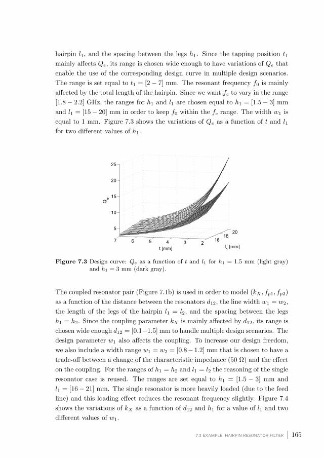
hairpin l1, and the spacing between the legs h1. Since the tapping position t1

mainly affects Qe, its range is chosen wide enough to have variations of Qe that

enable the use of the corresponding design curve in multiple design scenarios.

The range is set equal to t1 = [2− 7] mm. The resonant frequency f0 is mainly

affected by the total length of the hairpin. Since we want fc to vary in the range

[1.8− 2.2] GHz, the ranges for h1 and l1 are chosen equal to h1 = [1.5− 3] mm

and l1 = [15− 20] mm in order to keep f0 within the fc range. The width w1 is

equal to 1 mm. Figure 7.3 shows the variations of Qe as a function of t and l1

for two different values of h1.

Figure 7.3 Design curve: Qe as a function of t and l1 for h1 = 1.5 mm (light gray)and h1 = 3 mm (dark gray).

The coupled resonator pair (Figure 7.1b) is used in order to model (kX , fp1, fp2)

as a function of the distance between the resonators d12, the line width w1 = w2,

the length of the legs of the hairpin l1 = l2, and the spacing between the legs

h1 = h2. Since the coupling parameter kX is mainly affected by d12, its range is

chosen wide enough d12 = [0.1−1.5] mm to handle multiple design scenarios. The

design parameter w1 also affects the coupling. To increase our design freedom,

we also include a width range w1 = w2 = [0.8−1.2] mm that is chosen to have a

trade-off between a change of the characteristic impedance (50 Ω) and the effect

on the coupling. For the ranges of h1 = h2 and l1 = l2 the reasoning of the single

resonator case is reused. The ranges are set equal to h1 = [1.5 − 3] mm and

l1 = [16− 21] mm. The single resonator is more heavily loaded (due to the feed

line) and this loading effect reduces the resonant frequency slightly. Figure 7.4

shows the variations of kX as a function of d12 and h1 for a value of l1 and two

different values of w1.

7.3 EXAMPLE: HAIRPIN RESONATOR FILTER 165

Figure 7.4 Design curve: kX as a function of h1 and d12 for l1 = 19.75 mm andw1 = 0.8 mm (light gray) and w1 = 1.2 mm (dark gray).

All numerical experiments use Matlab R2014A and ADS Momentum EM solver

[ADS 14] and run on a Windows platform equipped with Intel Core i7 − 4770

3.40GHz CPU and 8 GB RAM.

The metamodels for this example describe the output variables (M,fp1, fp2)

and (Qe, f0) as a function of the corresponding input variables (geometrical

design parameters) defined above. The metamodels are generated using the

sparse grid interpolation schemes with adaptive sampling proposed in [Klim 05;

Klim 07]. The quality of the metamodels is judged based on an error measure.

It is defined as the absolute error of the modeled quantity (e.g. M) divided

by the difference between the maximum and minimum value of this quantity

over the range for which the quantity is modeled. A maximum error equal

to 0.01 is desired. We have used the built-in adaptive frequency sampling of

the ADS Momentum [ADS 14] to efficiently sample the scattering parameters

response of the coupled resonator and single loaded resonator structures in the

frequency-domain. The Vector Fitting system identification method [Gust 99]

has been used to build pole-residue rational models of S21(j2πf) and S11(j2πf)

of these two structures. These rational models have been evaluated over a dense

frequency grid of 1001 samples to extract the response variables data samples of

(M,fp1, fp2) and (Qe, f0). This is repeated at each value of the design parameters

chosen by the adaptive sampling process [Klim 05; Klim 07] in the design space.

The adaptive sampling method [Klim 05; Klim 07] has required 157 samples

to generate the metamodels of (M,fp1, fp2) and 121 samples for the model of

(Qe, f0) with a maximum error equal to 0.01. The average CPU time needed to


METAMODELS

extract the data samples of (M,fp1, fp2) and (Qe, f0) in a design space point from

EM simulations (with adaptive frequency sampling and Vector Fitting models)

is equal to 7.4 s and 3.8 s respectively. The overall CPU time needed to build

the metamodels of (M,fp1, fp2) and (Qe, f0) is equal to 20 m 4 s and 6 m 47 s,

respectively.

The average CPU time needed to evaluate the built metamodels of (M,fp1, fp2)

and (Qe, f0) in a design space point is equal to 0.64 ms and 0.28 ms. When we

compare this to the classical design curves generation method to generate 4-D

design curves on regular grid for (M,fp1, fp2) taking 5 samples for each design

parameter in the design space (d12, w1 = w2, l1 = l2, h1 = h2), this would already

require 54 = 625 samples (therefore 625 EM simulations). This is more than two

times the amount of samples needed to generate the metamodels of (M,fp1, fp2)

and (Qe, f0) with the proposed approach. Moreover, in the classical approach

the user has no idea whether the frequency axis and the design space are over-

or under-sampled and has no clue about the level of accuracy achieved.

The 4-D and 3-D metamodel-based design curves of (M,fp1, fp2) and (Qe, f0)

are finally used to obtain design parameters values for three different design

scenarios with the following specifications:

1. Design 1 : fc = 1.9 GHz, FBW = 0.12, passband ripple = 0.1 dB (RL =

16.43 dB)

2. Design 2 : fc = 2 GHz, FBW = 0.8, passband ripple = 0.1 dB (RL =

16.43 dB)

3. Design 3 : fc = 2.1 GHz, FBW = 0.1, passband ripple = 0.1 dB (RL =

16.43 dB)

Figure 7.5 shows the scattering parameters of the 5-th order filter after an ini-

tial dimensioning based on the metamodel-based design curves for each design

scenario. In the three design scenarios, the difference between the desired and

actual FBW is less than 0.005 and there is a small shift of the center frequency

fc. When we compare these results to other initial designs found in the liter-

ature [Hong 01], we observe a similar quality of the initial designs. In order

to have an idea of the difference between the implemented and ideal coupling

parameters in the bandpass domain we extract the coupling matrices using the

method discussed in Chapter 4. Table 7.1 compares the extracted and ideal

couplings for the 3 designs. For Design 1 we observe an maximum relative error

of 0.0428. The relative error on Qe is 0.0033. The frequency shift with respect


to fc explains the presence of non-zero self-couplings, which are relatively small.

For Design 2 we observe a similar relative error for the inter-resonator couplings

of 0.0169. The error on the external quality factor is 0.0362. There is also a

frequency shift, but this shift is smaller. Note that the inter-resonator couplings

are smaller for this example, because of the narrower bandwidth. This results in

larger distances between the resonators. Therefore the loading on the resonators

is smaller and thus the frequency shift is expected to be smaller. This is what we

observe. For Design 3 we find a relative error of 0.0313 for the inter-resonator

couplings and relative error 0.12 for the external quality factor. Nevertheless

this error is still acceptably small for an initial design value.

The fact that the curves are multi-dimensional allows the designer to use them

for several designs. An important parameter that is different for the three cases

is the length of the legs l1 and the distance between the legs h1 of the hairpin

resonator . These parameters also have an important effect on the coupling

and thus on the inter-resonator spacings. In the classical approach the inter-

resonator coupling curves would have to be re-extracted for every new value of

l1 and h1.

Design 1 Design 2 Design 3Parameter Extracted Ideal Extracted Ideal Extracted IdealQe1 9.5251 9.5568 14.3352 13.8349 11.4681 13.0950Qe2 9.5251 9.5568 14.3352 13.8347 11.4681 13.0947M ′12 0.0998 0.0957 0.0638 0.0649 0.0797 0.0823M ′23 0.0737 0.0729 0.0486 0.0492 0.0608 0.0627M ′34 0.0732 0.0729 0.0486 0.0492 0.0608 0.0627M ′45 0.0997 0.0957 0.0638 0.0649 0.0797 0.0823M ′11 0.0285 0 0 0.0197 0 0.0299M ′22 0.0269 0 0 0.0049 0 0.0130M ′33 0.0222 0 0 0.0113 0 0.0050M ′44 0.0335 0 0 0.0034 0 0.0152M ′55 0.0285 0 0 0.0197 0 0.0299

Table 7.1 Extracted and ideal coupling parameters in the bandpass domain for thethree designs.


METAMODELS

(a) |S11| for the different initial designs.

(b) |S21| for the different initial designs.

Figure 7.5 |S11| and |S21| for the initial values of the different design scenarios.


7.4 Conclusion

This chapter introduces a metamodeling approach for an efficient and automated

generation of multidimensional design curves for coupled-resonator bandpass

filters. Adaptive sampling approaches are used to minimize the number of EM-

simulations and the number of frequency samples per EM-simulation needed to

generate the metamodels that represent the design curves. The only required

user interaction is the choice of the ranges of the frequency and of the design

parameters. Large variations of multiple design parameters can be taken into

account, which allows one to use the design curves in multiple design scenarios.

These large variations come at a cost of a higher time to generate the curves. Also

when the number of design parameters grows, the time needed to generate the

curves increases very fast as well. This is known as the curse of dimensionality.

In this application however the number of design parameters is typically low,

since the filter is divided into its individual building blocks and each block is

modeled separately.

The numerical results have confirmed the efficiency, accuracy and flexibility of

the proposed methodology. Multidimensional design curves based on efficient

metamodels whose generation is fully automated are a powerful design tool that

allows designers to efficiently explore multiple design scenarios and significantly

save computational resources during the design flow.


METAMODELS

8A Scalable Macromodeling Methodology for the Efficient Design of Mi-

crowave Filters

This chapter introduces a novel computer-aided design (CAD) methodology for

microwave filters. The methodology uses scalable macromodels to model the

behavior of the S-parameters as a function of the physical design parameters

of the filter. The physical parameters are varied over a well chosen range of

values. The benefit of a scalable macromodel is that they are numerically cheap

to evaluate. Once the model is generated, it can thus be used to optimize the

filter design parameters to meet the specifications. If the ranges of the design

parameters are chosen sufficiently broad, the model can be reused in multiple

design scenarios. So far the inclusion of scalable macromodels in the design cycle

of microwave filters has not been studied and discussed in the literature.

In this chapter, we show that scalable macromodels can be included in the design

cycle of microwave filters and can be reused in multiple designs at a low com-

putational cost. We give guidelines to properly generate and use these scalable

macromodels in a filter design context. We illustrate the approach on a state-

of-the-art design example: a microstrip dual-band bandpass filter with closely

spaced passbands and a complex geometrical structure. The results confirm that

scalable macromodels can indeed be used as proper design tools and represent

an efficient and accurate alternative to the mainstream, but computationally

expensive EM simulator-based design flow. The work discussed in this chapter

has been published in [Caen 16].

8.1 Introduction

Over the last years several methods have been developed to improve the design

of microwave filters [Levy 02; Swan 07a]. Design techniques based on design

curves are shown to yield relatively good initial designs. However most de-

171

sign curve based filters, require post-processing and fine-tuning to meet the

desired frequency template specifications. The fine-tuning process involves nu-

merical optimization and is based on multiple accurate electromagnetic (EM)

simulations. Accuracy comes at a price however, these solvers are known to

be computationally expensive and hence time consuming. Even though most

optimization methods [Band 94b; Arnd 04; Koza 02; Lamp 04; Koza 06] yield

accurate designs, their design time grows linearly with the number of filters to

be designed. Even though the layout if similar. This is a consequence of the

optimization towards a single set of specifications. If the specifications change,

the complete process must be redone.

To speed up the design process, we propose to replace the EM solver by a com-

putationally efficient scalable frequency response macromodel. In this chapter,

scalable (or parametric) macromodels are used as a compromise between model

accuracy and complexity. Generating scalable macromodels to represent the

parameterized response of microwave systems as a function of frequency and

additional design parameters such as geometrical variables and material proper-

ties, is an active field of research [Peik 98; Lame 03; Cuyt 06; Deva 03; Lame 09;

Basl 10; Lehm 01; Triv 09; Ferr 09; Ferr 10; Triv 10; Ferr 11; Ferr 12]. The two

main advantages of using scalable macromodels in the design process are:

1. The scalable macromodels replace the expensive EM solver to evaluate the

filter response as a function of the frequency and the design parameters

of interest (e.g. geometrical parameters) over certain predefined ranges.

Therefore, these scalable macromodels can be used in different optimiza-

tion scenarios where changes in the specifications of the filter (e.g. the

bandwidth of interest, the selectivity, etc.) need to be examined.

2. The scalable macromodels can also be used to speed up other computa-

tionally expensive design activities, such as design exploration and design

variability analysis. Design space exploration leads to an understanding

of the filter behavior with respect to design parameters. Design variabil-

ity analysis evaluates the system reliability. Since macromodels are quite

cheap to evaluate and also accurate enough to properly capture the effects

of the design parameter variations on the filter frequency response, they

increase the time-efficiency of these design tasks.

Even though the extraction of scalable macromodels can easily be automated

using sequential sampling approaches [Chem 14b], it still requires the designer

to specify additional information. For example, the designer must select ranges

172 CHAPTER 8 A SCALABLE MACROMODELING METHODOLOGY FOR THE EFFICIENT DESIGN OF MICROWAVE

FILTERS

for the design parameters, for which the model is then built to be accurate over

these ranges. For a first design the model must thus be extracted during the

design process itself. Note that once it is extracted it can be used to optimize

filters having the same physical structure for different design specifications.

In this chapter, we show how to include scalable macromodels in the design cycle

of microwave filters. We give guidelines to properly generate and use scalable

macromodels in a filter design context. The focus is put on the practical use of

scalable macromodels for design purposes. We show that scalable macromodels

can be reused to optimize the design of different filters to meet multiple sets

of specifications. This distinguishes the proposed method from existing model-

based optimization methods and breaks the linear growth of the extraction time

with respect to the number of designs. This is a major difference with respect to

the approach used in [Kozi 06; Kozi 10b; Kozi 10a; Couc 10; Couc 12] that aims

at optimizing a particular performance measure for a particular design. This

leads to restart the modeling step for optimization each time the specifications

are changed. To summarize, this chapter explains how scalable macromodels

can effectively and practically be used by designers to speed-up the design flow,

while still achieving accurate results.

We have chosen a state-of-the-art design example: a microstrip dual-band band-

pass filter described as it is described in [Hsu 13] is used to illustrate our ap-

proach. In [Hsu 13], a design method is presented to adjust the center frequency,

the bandwidth, the position of the transmission zeros and the desired ratio of

the resonant frequency of the two passbands. This filter consists of two coupled

unequal length shunted-line stepped impedance resonators. The example nicely

illustrates the proposed macromodel-based design approach, since the design

parameters are all coupled and optimization of the design is therefore necessary

on all parameters simultaneously.

Section 8.2 describes a state-of-the-art scalable macromodeling method for an

automated model generation. To speed-up the generation process, a sampling

algorithm [Chem 14b] is used to gather data samples located at spots in the

design space where the response changes rapidly.

8.2 Scalable Macromodels for Microwave Filters

This section introduces a state-of-the-art scalable macromodeling technique that

is coupled to a sequential sampling algorithm to obtain an automated model

generation framework for microwave filters.

8.2 SCALABLE MACROMODELS FOR MICROWAVE FILTERS 173

8.2.1 BUILDING A SCALABLE MACROMODEL FROM DATA SAMPLES GENERATED BY EM

SOLVERS

The first step needed for the scalable macromodeling process is to generate

data samples used to train the model. A set of multivariate data samples

(sn, gk),H(sn, gk) (n ∈ 1, . . . , nF , k ∈ 1, . . . , ng) represents a set of

parameter-dependent frequency-domain responses. This data set depends on

the Laplace variable or complex frequency s = jΩ = j2πf and also on an

additional set of ng physical design variables g = (g1, . . . , gng ). Note that f is

the physical frequency in the bandpass domain. The region in the parameter

space that contains the selected parameters g is called the design space.

For filter structures, these design variables describe the geometry of the system

that a designer varies during the design. The data samples (sn, gk),H(sn, gk)are used to generate a scalable macromodel. The model needs to be able to

efficiently and accurately describe the parameterized behavior of the system

under study.

Similarly to what was done in Chapter 7 the data samples are divided into two

datasets: an estimation set and a validation set. The estimation set is utilized

to build a scalable macromodel. The validation set is used to validate the model

accuracy in design space points that were not used for the model generation. An

efficient sampling algorithm [Chem 14b] is used to gather data samples located at

maximally informative design space positions automatically. Spots in the design

space where the response changes rapidly are sampled more densely, while the

total number of data samples is minimized as much as possible. The algorithm

is briefly described in Section 8.2.2. In [Chem 14b], the sequential sampling

algorithm is used to automatically gather the data for the generation of scalable

macromodels [Ferr 11; Ferr 12]. These modeling methods [Ferr 11; Ferr 12] are

based on the use of interpolation of transfer functions and the use of scaling

coefficients. Recently, a scalable macromodeling approach has been proposed

in [Chem 14a] to enhance the modeling capability of [Ferr 11; Ferr 12] by using

multiple frequency scaling coefficients.

In this work, we use the scalable macromodeling technique [Chem 14a] and com-

bine it with the sequential sampling method [Chem 14b]. This is an important

step to allow automating the generation of scalable macromodels and reducing

the effort and prior knowledge needed by designers to use scalable macromodels

as a design tool. The corresponding main modeling steps are recalled briefly

in what follows. The reader can refer to [Ferr 11; Ferr 12; Chem 14a] for a

more detailed explanation. The idea is to use ng dimensional hyper-rectangular


FILTERS

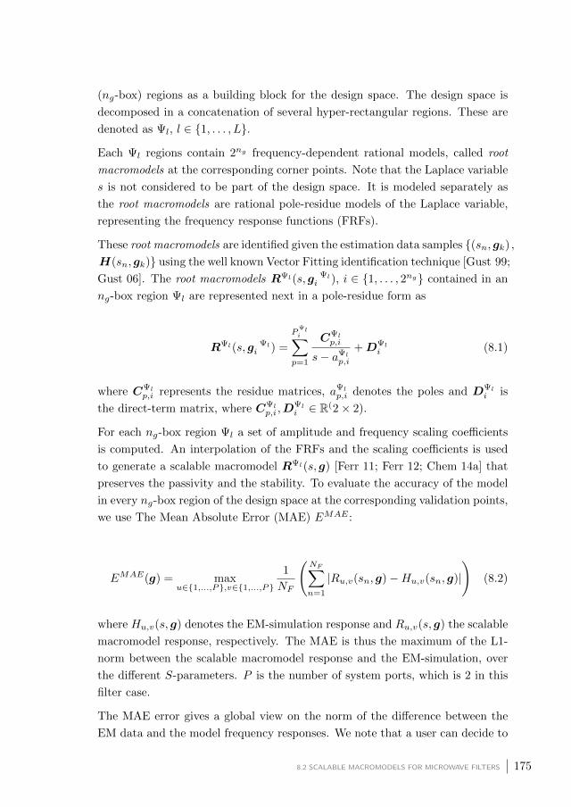
(ng-box) regions as a building block for the design space. The design space is

decomposed in a concatenation of several hyper-rectangular regions. These are

denoted as Ψl, l ∈ 1, . . . , L.

Each Ψl regions contain 2ng frequency-dependent rational models, called root

macromodels at the corresponding corner points. Note that the Laplace variable

s is not considered to be part of the design space. It is modeled separately as

the root macromodels are rational pole-residue models of the Laplace variable,

representing the frequency response functions (FRFs).

These root macromodels are identified given the estimation data samples (sn, gk) ,

H(sn, gk) using the well known Vector Fitting identification technique [Gust 99;

Gust 06]. The root macromodels RΨl(s, g Ψli ), i ∈ 1, . . . , 2ng contained in an

ng-box region Ψl are represented next in a pole-residue form as

RΨl(s, g Ψli ) =

PΨli∑

p=1

CΨlp,i

s− aΨlp,i

+DΨli (8.1)

where CΨlp,i represents the residue matrices, aΨl

p,i denotes the poles and DΨli is

the direct-term matrix, where CΨlp,i ,D

Ψli ∈ R(2× 2).

For each ng-box region Ψl a set of amplitude and frequency scaling coefficients

is computed. An interpolation of the FRFs and the scaling coefficients is used

to generate a scalable macromodel RΨl(s, g) [Ferr 11; Ferr 12; Chem 14a] that

preserves the passivity and the stability. To evaluate the accuracy of the model

in every ng-box region of the design space at the corresponding validation points,

we use The Mean Absolute Error (MAE) EMAE :

EMAE(g) = maxu∈1,...,P,v∈1,...,P

1

NF

(NF∑

n=1

|Ru,v(sn, g)−Hu,v(sn, g)|)

(8.2)

where Hu,v(s, g) denotes the EM-simulation response and Ru,v(s, g) the scalable

macromodel response, respectively. The MAE is thus the maximum of the L1-

norm between the scalable macromodel response and the EM-simulation, over

the different S-parameters. P is the number of system ports, which is 2 in this

filter case.

The MAE error gives a global view on the norm of the difference between the

EM data and the model frequency responses. We note that a user can decide to

8.2 SCALABLE MACROMODELS FOR MICROWAVE FILTERS 175

utilize another error measure that is more suitable to his modeling needs. If a

fixed set of estimation and validation data samples is available, each region Ψl

in the design space is modeled and the corresponding model is validated. The

complete design space is covered cell by cell. In the next section, we briefly

describe the sequential sampling method [Chem 14b; Chem 14a] that is used to

automate the generation of scalable macromodels.

8.2.2 AUTOMATED DESIGN SPACE SAMPLING USING SEQUENTIAL SAMPLING

The sequential sampling algorithm [Chem 14b] used in this work simultaneously

automates the generation of scalable macromodels [Chem 14a] and reduces the

computational effort needed to gather estimation and validation data samples.

Figure 8.1 shows the flowchart of the algorithm. The different steps are discussed

below:

1. Initialization: defines the design space. The ng dimensional vector design

parameters is labeled g = (g1, . . . , gng ). The initial design space is a hyper

rectangle bound by 2ng corner points. It forms one single ng-box region

Ψl with l = L = 1, where L is the number of hyper rectangles that divide

the complete design space.

2. Scalable macromodel extraction : A scalable macromodel RΨl(s, g) is built

for each elementary region Ψl (l ∈ 1, . . . , L) (see Section 8.2.1).

3. Model validation: The model response in the selected region Ψl is validated

with respect to the actual EM-solver response. This requires a set of

validation data points, with corresponding EM simulations that are not

used for the model estimation. This is done in two steps: first the response

of the EM solver is compared with the macromodel response evaluating

using the MAE measure (8.2) at the center of the maximal dynamic edge.

The maximal dynamic edge is the edge for which the difference between the

response in the corresponding corner points is the greatest. If the model

is accurate enough, a second level of accuracy check is performed at the

geometric center of the hyper rectangle (similarly to [Chem 14b]).

4. Refinement : If the accuracy of the model in the region Ψl is below the

threshold ∆Ψ, the region Ψl is not divided further. Otherwise, the region

is split into two subregions along the maximally sensitive edge [Chem 14b].

The accuracy threshold ∆Ψ can be decided based on the design specifica-

tions set by the user. The threshold ∆Ψ must thus be specified by the


FILTERS

user. For example, if a minimal stopband attenuation of 30 dB is required

for the optimal design, the scalable macromodel should reach an accuracy

of at least −30 dB.

After updating the total number of regions L the algorithm is repeated from Step

2 on until all regions Ψl are covered with the required accuracy level, i.e. l = L.

Figure 8.1 shows a schematic overview of the sequential sampling algorithm.

Figure 8.1 Flowchart of the sequential sampling algorithm.

8.3 Including the Scalable Macromodel in the Design Process

As we have seen in Chapter 3, design curves are often used to obtain initial

values for the physical design parameters of the filter. Due to second order effects

most initial designs require post-processing and fine-tuning to meet the desired

specification. This process involves numerical optimization and is classically

based on multiple, accurate EM-simulations. In Chapter 5 and Chapter 6, we

have introduced novel tuning methods for coupled resonator based bandpass

filters. Although the methods yield accurate designs, they still require several

EM-simulations. The alternative that is explained here starts from the following

idea: Rather than investing time in the tuning or optimization, we may invest

that time to extract a scalable macromodel. Although the model generation

process is automated, some judicious user choices are still required:

• The frequency range of interest has to be chosen.

• The physical parameters of the filter have to be chosen (the choice of g).

Typically ng parameters are chosen in order to maximally influence the

8.3 INCLUDING THE SCALABLE MACROMODEL IN THE DESIGN PROCESS 177

properties of the filter response that do not meet the specifications. For

example, when the center frequency of the filter is too high, the physical

length of the resonators is certainly included.

• The ranges of variation of the design parameters must also be set. These

ranges depend on practical and/or physical considerations. To make this

less abstract, let us consider the spacing between two microstrip lines in

a coupled line pair. When the spacing is too small, the design cannot

be realized physically due to fabrication tolerances. When the spacing

becomes too large, there is no more coupling between the lines.

• Another important choice is the desired accuracy of the macromodel. This

choice depends on the filter specifications. For example, when the required

minimal attenuation is equal to −20 dB, the scalable macromodel should

be able to describe the filter characteristics up to an accuracy of at least

−20 dB. The user may decide to increase the model accuracy to include

some safety margin (e.g. from 5 to 10 dB of margin).

As their name suggests, user choices depend on the design and must thus be

made by the user after the initial design step. Once the model is generated it

is used to optimize the initial design. On top of that, the model can also be

used to gain insights about the behavior of the filter with respect to the design

parameters or used to optimize a new filter for a different set of specifications.

The macromodel based optimization is explained in the next section.

8.4 Macromodel based Optimization

The scalable macromodel R(s, g) of a microwave filter can be used to optimize

the initial design such that it fulfills the desired specifications. The global opti-

mization function MultiStart in Matlab is used in this chapter to perform global

optimization of the filter to satisfy the desired performances. The geometrical

values obtained during the initial dimensioning of the filter are used as starting

point for the optimization. In order to avoid local minima, the MultiStart rou-

tine also generates uniformly distributed starting points in the design space from

which several local optimizer runs are performed, generating multiple solutions.

This routine then ranks the solutions in terms of their cost function values in

ascending order. It is important to highlight that a global optimization usually

requires a high number of function evaluations (and then simulations of the sys-

tem behavior). This is not computationally expensive if scalable macromodels


FILTERS

are used for it. Global optimization is interesting since it searches for design

solutions over the complete design space of interest.

First we choose a frequency grid for which the scalable macromodel R(sm, g)

is evaluated during the optimization. A frequency in this grid is denoted as

sm, where m ∈ 1, 2, . . . , nOptF and nOptF is the number of frequencies in the

grid. These frequencies are chosen in the stop and passbands of the filter. The

frequency template specifies a lower frequency response threshold RmL and a

upper frequency response threshold RmU at frequency samples sm. The scalable

macromodel allows to calculate whether the filter satisfies or violates the given

specification by calculating:

F (sm, g) = RmL −R(sm, g) or R(sm, g)−RmU . (8.3)

A negative value in (8.3) indicates that the corresponding specification is satis-

fied, while a positive value denotes that the specification is violated. Note that

the evaluation of the macromodel in (8.3) is numerically cheap. The cost function

that the optimization minimizes in this chapter is the worst-case violation over

all the S-parameters matrix entries and the sm samples

F (g) = maxi,j

maxsm

Fi,j(sm, g). (8.4)

where Fi,j represents the cost function for the (i, j) − th S-parameter matrix

entry. Note that this is the same cost function as the one used in [Band 94b].

The cost function (8.4) is then supplied to the MultiStart optimization routine,

resulting in multiple optimal design space points that satisfy the specifications.

The application to a filter case is illustrated in Section 8.5. Note that in the

literature several more suitable cost functions exist [Came 07b; Band 88] and

that the scalable macromodel can also be used to optimize other cost functions.

8.5 Example: Microstrip Dual-Band Bandpass Filter

We have chosen the dual-band bandpass microstrip filter described in [Hsu 13] to

illustrate and validate the proposed approach. The filter consists of two coupled

unequal length shunted-line stepped impedance resonators (Figure 8.2). We use

the design method presented in [Hsu 13] to obtain initial values of the design

parameters for the initial design.

The filter is fabricated on a RO4003 substrate with a relative permittivity εr

8.5 EXAMPLE: MICROSTRIP DUAL-BAND BANDPASS FILTER 179

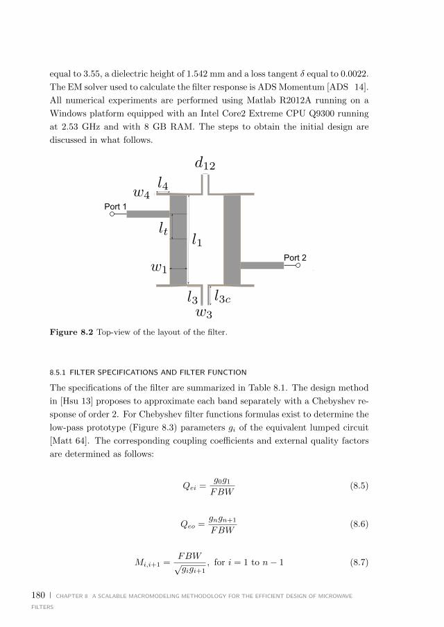
equal to 3.55, a dielectric height of 1.542 mm and a loss tangent δ equal to 0.0022.

The EM solver used to calculate the filter response is ADS Momentum [ADS 14].

All numerical experiments are performed using Matlab R2012A running on a

Windows platform equipped with an Intel Core2 Extreme CPU Q9300 running

at 2.53 GHz and with 8 GB RAM. The steps to obtain the initial design are

discussed in what follows.

Figure 8.2 Top-view of the layout of the filter.

8.5.1 FILTER SPECIFICATIONS AND FILTER FUNCTION

The specifications of the filter are summarized in Table 8.1. The design method

in [Hsu 13] proposes to approximate each band separately with a Chebyshev re-

sponse of order 2. For Chebyshev filter functions formulas exist to determine the

low-pass prototype (Figure 8.3) parameters gi of the equivalent lumped circuit

[Matt 64]. The corresponding coupling coefficients and external quality factors

are determined as follows:

Qei =g0g1

FBW(8.5)

Qeo =gngn+1

FBW(8.6)

Mi,i+1 =FBW√gigi+1

, for i = 1 to n− 1 (8.7)


FILTERS

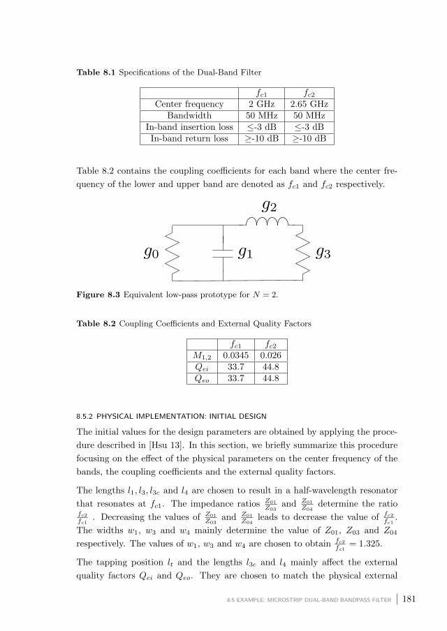
Table 8.1 Specifications of the Dual-Band Filter

fc1 fc2Center frequency 2 GHz 2.65 GHz

Bandwidth 50 MHz 50 MHzIn-band insertion loss ≤-3 dB ≤-3 dBIn-band return loss ≥-10 dB ≥-10 dB

Table 8.2 contains the coupling coefficients for each band where the center fre-

quency of the lower and upper band are denoted as fc1 and fc2 respectively.

Figure 8.3 Equivalent low-pass prototype for N = 2.

Table 8.2 Coupling Coefficients and External Quality Factors

fc1 fc2M1,2 0.0345 0.026Qei 33.7 44.8Qeo 33.7 44.8

8.5.2 PHYSICAL IMPLEMENTATION: INITIAL DESIGN

The initial values for the design parameters are obtained by applying the proce-

dure described in [Hsu 13]. In this section, we briefly summarize this procedure

focusing on the effect of the physical parameters on the center frequency of the

bands, the coupling coefficients and the external quality factors.

The lengths l1, l3, l3c and l4 are chosen to result in a half-wavelength resonator

that resonates at fc1. The impedance ratios Z01

Z03and Z01

Z04determine the ratio

fc2fc1

. Decreasing the values of Z01

Z03and Z01

Z04leads to decrease the value of fc2

fc1.

The widths w1, w3 and w4 mainly determine the value of Z01, Z03 and Z04

respectively. The values of w1, w3 and w4 are chosen to obtain fc2fc1

= 1.325.

The tapping position lt and the lengths l3c and l4 mainly affect the external

quality factors Qei and Qeo. They are chosen to match the physical external


quality factors approximately to the ones found during the realization step. Ini-

tial values for these parameters are difficult to determine, as they affect the

response of both bands. The physical Qei and Qeo are shown in Table 8.3.

Note that these quality factors are extracted using (3.19) at ωc1 = 2πfc1 and

ωc2 = 2πfc2 separately, neglecting the influence of the bands on each other.

The spacing parameter d12 between the resonators mainly affects the coupling

coefficient M12. w3 and w4 also affect the coupling coefficient, but their effect is

smaller. The values of d12, w3 and w4 are chosen such that the physical coupling

coefficient M12 is approximately equal to the value found during the realization

step. The physical M12 for both bands is shown in Table 8.3. These parameters

are extracted using (3.11) for each band separately.

Table 8.3 Coupling Coefficients and External Quality Factors (EM simulations)

fc1 fc2M1,2 0.0373 0.0327Qei 25 33.5Qeo 25 33.5

The initial value of the design parameters given by this design method are sum-

marized in Table 8.4. Figure 8.4 shows the magnitude of S21 and S11 for the

initial design, respectively. It is clear that the specifications are not met and

therefore optimization is needed.

Table 8.4 Initial Values of the Design Parameters

l1 24.5 mml3 17 mml3c 10 mml4 1.5 mmlt 8.8 mmw1 9.5 mmw3 1 mmw4 1 mmd12 1.62 mm

8.5.3 DESIGN SPACE

In this section, we describe how to select the physical parameters that become

design parameters. Figure 8.4b shows that the ratio fc2fc1

is not equal to 1.325.

But f1 = 2 GHz is indeed properly realized. As the ratio fc2fc1

is mainly affected byZ01

Z03and Z01

Z04, w1 and w3 = w4 are chosen as design parameters. The ranges are


FILTERS

1.5 2 2.5 3

−30

−20

−10

0

Frequency (GHz)

|S11|(

dB

)

(a) |S11| for the initial design (—) and specifications (—).

1.5 2 2.5 3−60

−40

−20

0

Frequency (GHz)

|S21|(

dB

)

(b) |S21| for the initial design (—) and specifications (—).

Figure 8.4 |S11| and |S21| for the initial design and the specifications.

determined as follows: w1 must not become too large, because for large values

of w1 the characteristic impedance Z01 does not decrease anymore. Hence, it

is not relevant to model the filter behavior for those values. The value of w1

must not become too small either, because then the ratio Z01

Z03then becomes too

large and fc2fc1

becomes too large. The value of w3 must not become too small,

because then it is not physically realizable. It must also not become too large,


because then the ratio Z01

Z03becomes too large and fc2

fc1becomes too large. Since

the coupling coefficient between the resonators is too large in the design, d12 is

also chosen as a design parameter. The upper bound of the range of d12 (= 2

mm) is chosen to ensure that there is still electromagnetic coupling between the

resonators and the lower bound (=0.5 mm) is chosen such that it is physically

realizable. Table 8.5 contains the ranges of the design parameters.

Table 8.5 Ranges of the design parameters.

Parameter Range

w1 8.5-10.5 mmw3 0.5-2 mmd12 0.5-2 mm

8.5.4 GENERATION OF THE SCALABLE MACROMODEL

Section 8.2.1 and Section 8.2.2 show that the generation of scalable macromodels

is an automated process. Nevertheless, the user has to specify the design space,

the frequency span and the accuracy for the model. The choice of the design

space g = [w1, w2, d12] has been previously discussed. The frequency span is

chosen equal to f ∈ [1.3 − 3.3] GHz to be wide enough to contain the filter

behavior of interest within it. The choice of the model accuracy is based on the

minimal attenuation desired in the stopband that is set equal to 30 dB in this

numerical example. The accuracy of the scalable macromodel has been set to

−30 dB based on the MAE measure (8.2).

The scalable macromodeling method of [Chem 14a] discussed in Section 8.2.2

has been implemented in Matlab R2012a and used to drive the Momentum

software with Adaptive Frequency Sampling (AFS) [ADS 14] to generate the

S-parameters at selected design space samples. AFS is a technique included in

ADS2011 Momentum that adaptively samples the frequency range and can be

used to efficiently provide the system response for a specified number of samples,

that are chosen freely in the band. The number of simulated frequency samples

nF obtained by AFS over the range f ∈ [1.3−3.3] GHz has been chosen equal to

301 to build the scalable macromodel. The steep changes in the behavior of the

S-parameters of the microwave filter with respect to frequency are hence well

captured.

The MAE (8.2) is used to asses the accuracy of the scalable macromodel. Ta-

ble 8.6 reports the total number of design space samples (estimation and vali-

dation), the worst case MAE (8.2) over the estimation and validation data, the


FILTERS

Table 8.6 Scalable macromodeling

# Samples CPU Time AccuracyGeneration Validation Modeling Data Gen. [dB]

72 45 36 min 35 s 1 h 55 min 21 s −30.48Average CPU Time for one ADS frequency sweep = 50 sAverage CPU Time for one macromodel frequency sweep = 19.5 msSpeed-up = 2564×

CPU time needed to run all the ADS Momentum estimation and validation sim-

ulations and the CPU time needed to obtain the scalable macromodel using the

sequential scheme coupled with the scalable macromodeling method [Chem 14a].

The average CPU time needed by ADS Momentum (using AFS) and the scalable

macromodel for one frequency sweep over 301 frequency points is also shown in

Table 8.6. This measure is crucial to judge the potential advantage of the pro-

posed approach for efficient design optimizations when compared to the direct

use of EM-based optimization schemes.

8.5.5 FILTER OPTIMIZATION

The scalable macromodel is used to perform multiple optimizations for this filter.

The optimization specifications on the S-parameters of the filter under study are:

|S21| < −LA1 dB fs1 ≤ f ≤ fs2, (8.8a)

|S21| > −LIL dB fp1 ≤ f ≤ fp2, (8.8b)

|S11| < −LRL dB fp1 ≤ f ≤ fp2, (8.8c)

|S21| < −LA2 dB fs3 ≤ f ≤ fs4, (8.8d)

|S21| > −LIL dB fp3 ≤ f ≤ fp4, (8.8e)

|S11| < −LRL dB fp3 ≤ f ≤ fp4, (8.8f)

|S21| < −LA3 dB fs5 ≤ f ≤ fs6. (8.8g)

with three optimization cases:


Table 8.7 Dual-band bandpass filter: global optimization results using the macro-model.

Initial design Best optimal design # Function OptimizationCase (w1, w2, d12) (mm) (w∗1 , w

∗2 , d∗12) (mm) evaluations time

I [9.5, 1, 1.62] [9.66, 1, 1.44] 6557 5 min, 40 s

II [9.5, 1, 1.62] [10.4, 1.17, 1.38] 5456 5 min, 47 s

III [9.5, 1, 1.62] [10.3, 1.43, 1.25] 6675 5 min, 43 s

I.(fs1, fs2, fp1, fp2, fs3, fs4, fp3, fp4, fs5, fs6) =

(1.3, 1.7, 1.975, 2.025, 2.275, 2.325, 2.625, 2.675, 2.9, 3.3) GHz,

(LA1, LIL, LRL, LA2, LA3) = (−20,−3,−10,−20,−20) dB (8.9a)

II. (fs1, fs2, fp1, fp2, fs3, fs4, fp3, fp4, fs5, fs6) =

(1.3, 1.7, 1.975, 2.025, 2.275, 2.325, 2.625, 2.675, 2.9, 3.3) GHz,

(LA1, LIL, LRL, LA2, LA3) = (−20,−3,−10,−30,−20) dB (8.9b)

III. (fs1, fs2, fp1, fp2, fs3, fs4, fp3, fp4, fs5, fs6) =

(1.3, 1.6, 1.9, 1.95, 2.175, 2.25, 2.625, 2.675, 2.9, 3.3) GHz,

(LA1, LIL, LRL, LA2, LA3) = (−20,−3,−10,−20,−20) dB (8.9c)

As explained in Section 8.4, the global optimization function MultiStart in Mat-

lab R2012a is used to perform a global optimization with a cost function defined

in (8.4) using the previous specifications. 30 starting points are used for each

optimization case. For each optimization case, the function MultiStart found

multiple possible optimization solutions [w∗1 , w∗3 , d∗12] that satisfy the correspond-

ing specifications. The results of the three optimization cases are tabulated in

Table 8.7, where the best optimization solutions, the total number of function

evaluations and CPU time needed for the three global optimizations are shown.

Considering the average CPU time that is needed for one frequency sweep using

the EM solver and the scalable macromodel (see Table 8.6) and the number of

functions evaluations needed to perform the global optimizations in Table 8.7,


FILTERS

clearly shows that using the scalable macromodel allows a very efficient multiple

global optimization. The initial computational effort needed to generate the

scalable macromodel (see Table 8.6) becomes small compared to the CPU time

that is saved to perform the multiple global optimizations is considered.

Figure 8.5 shows the optimization results for Case I : The S-parameters are

shown before and after the optimization. The solid black lines show the spec-

ifications. From the two figures it is clearly seen that all the specifications are

satisfied. Similar results are for Case II and Case III as shown in Figure 8.6

and Figure 8.7. The green response curves denote the Momentum simulations

performed at the optimal solution points to verify that the model prediction (red

curves) is accurate. Note that there is a difference between the evaluation of the

macromodel and the EM-simulation for the optimized design. This difference is

however smaller than -30 dB, which is the error limit that was specified during

the the macromodel generation.

8.6 Discussion

Generating scalable macromodels becomes more computationally expensive with

an increasing number of design parameters. The so called ”curse of dimension-

ality” pops up in high-dimensional modeling problems. This affects two main

aspects of the modeling:

• the number of data samples needed to build and validate a model (and

then the CPU time to collect these data samples)

• The complexity (and then the CPU time) of the model generation when

the data samples are available

Working on fully regular design space grids to collect estimation and validation

data will make the complexity of the data to gathering increase in an exponential

way with respect to the number of design parameter. This issue can be mitigated

by using sequential sampling strategies that optimize the samples location in the

design space.

The modeling step for the technique [Chem 14a] will mainly suffer from an in-

creasing number of design parameters in the computation of the amplitude and

frequency scaling coefficients for each region of the design space. This issue can

be mitigated by exploiting parallelization strategies, since the scaling coefficients

computation for a design space region can be performed independently from the

other regions.

8.6 DISCUSSION 187

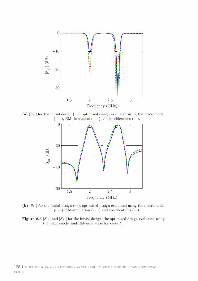
1.5 2 2.5 3

−30

−20

−10

0

Frequency (GHz)

|S11|(

dB

)

(a) |S11| for the initial design (—), optimized design evaluated using the macromodel(- - -), EM-simulation (- - -) and specifications (—).

1.5 2 2.5 3−60

−40

−20

0

Frequency (GHz)

|S21|(

dB

)

(b) |S21| for the initial design (—), optimized design evaluated using the macromodel(- - -), EM-simulation (- - -) and specifications (—).

Figure 8.5 |S11| and |S21| for the initial design, the optimized design evaluated usingthe macromodel and EM-simulation for Case I .


FILTERS

1.5 2 2.5 3−40

−30

−20

−10

0

Frequency (GHz)

|S11|(

dB

)


1.5 2 2.5 3−60

−40

−20

0

Frequency (GHz)

|S21|(

dB

)


Figure 8.6 |S11| and |S21| for the initial design, the optimized design evaluated usingthe macromodel and EM-simulation for Case II.

8.6 DISCUSSION 189

1.5 2 2.5 3−50

−40

−30

−20

−10

0

Frequency (GHz)

|S11|(

dB

)


1.5 2 2.5 3−60

−40

−20

0

Frequency (GHz)

|S21|(

dB

)


Figure 8.7 |S11| and |S21| for the initial design, the optimized design evaluated usingthe macromodel and EM-simulation for Case III.


FILTERS

8.7 Conclusion

In this chapter, we have introduced scalable macromodels in the design cycle of

microwave filters. We have discussed how to generate and use scalable macro-

models as a design tool for filters. The main advantage of these macromodels

is that they are cheap to evaluate with a suitable accuracy. Hence, the scalable

macromodels can replace the expensive EM solver during multiple optimizations

of the filter and then make these steps much less CPU time intensive. It is to be

noted that it also takes an initial computational effort to generate the macro-

model and that this must be done during the design cycle. However, this initial

computational effort that is needed to generate the scalable macromodel becomes

a little effort when the CPU time saved to perform multiple global optimizations

with respect to EM-based optimizations is considered. We have illustrated this

macromodeling-based design approach by applying it to the design of a state-

of-the-art microstrip dual-band bandpass filter. Although the generation of the

scalable macromodels is an automated process, it still requires some information

from a designer, namely the frequency span, the ranges of the design parameters

and the desired model accuracy. How a designer can hand this information to

the macromodel generation process has been explained in detail. We have finally

shown how the scalable macromodel can be used for multiple optimizations. The

corresponding numerical results confirm that the macromodeling-based design

approach works very well.

8.7 CONCLUSION 191

Conclusions

193

9Conclusions

In this work we investigate different model driven assisted design approaches for

the time-efficient design of microwave bandpass filters. We apply model assisted

design approaches not only to post-optimize the physical dimensions of the filter

but also to generate initial values for them.

In the first part of the thesis, we use a coupling matrix based approach. The

idea is to adjust the physical design parameters based on a comparison between

an extracted coupling matrix and the golden goal.

It is well known that coupling topologies may have multiple equivalent solutions

to the reconfiguration problem (Chapter 2). One of the main challenges is to

extract the physical solution starting from the simulated S-parameters of the

obtained design.

In Chapter 4 we develop a method that systematically extracts all possible solu-

tions corresponding to the implemented topology. We also propose a strategy to

model the second order effects (which are not included in the coupling topology

of the golden goal) by adding coupling parameters to the last row and column of

the extracted coupling matrix. The extraction of the coupling matrix of a mea-

sured SQ filter shows indeed that taking these second order effects into account

is indispensable to properly model the filter frequency response of the filter. We

also extract all the possible solutions for a CQ filter. This extraction shows

that from a mathematical point of view these solutions are equivalent. This

means that more information is required to identify the physically implemented

coupling matrix.

Chapter 5 shows that in the case of CQ and CT filters it is possible to identify the

physically implemented coupling matrix by applying some well chosen variations

to the physical structure of the filter. The main drawback of this approach is that

it requires several EM-simulations to determine the physical solution. We derive

195

an expression to predict how many EM-simulations (experiments) are required.

Once the physical solution is determined, we show that this knowledge allows

one to tune the filter. The extraction procedure only tells the user how far

the implemented coupling parameters are from the target values and not how

far the physical parameters are from their target values. As a consequence the

tuning procedure can still require a relatively high number of iterations for an

unexperienced designer to tune a filter.

Chapter 6 estimates the Jacobian matrix of the functional dependence of the

physically implemented coupling parameters to the design parameters using the

adjoint sensitivity of the S-parameters. Using the adjoint sensitivity provided by

the EM-simulator allows to estimate the Jacobian using only one EM-simulation.

Although including the adjoint sensitivity in such a simulation is numerically

more expensive, the method is more time-efficient in comparison to other tech-

niques based on finite difference extraction of the Jacobian matrix. A good

estimate of the Jacobian drastically reduces the number of iterations needed to

tune relatively complex filter structures. Another benefit of using the Jacobian

matrix is that it allows to determine the physically implemented coupling matrix

using only 1 EM-simulation.

In the second part of the thesis, we follow a metamodel based approach. The

main benefit of this kind of approach is that it generates accurate models for the

S-parameters or features of the S-parameters with an acceptably low number

of EM-simulations. These models are then used for 2 different kind of design

activities: the generation of initial values for the design parameters and the

post-optimization of the filter structures.

Chapter 7 automatically generates multidimensional design curves for the initial

dimensioning of coupled-resonator filters. The benefit of using a metamodel

approach with respect to the classical approach described in Chapter 3 is that

it requires a lower number of EM-simulations to cover a relatively wide range of

physical parameters. The multidimensional description allows to use the model

to generate initial values for multiple design scenarios.

Chapter 8 generates a scalable macromodel for a complex dual-band bandpass

filter. The benefit of a numerically much cheaper model when compared to the

EM-solver, is the speed of the optimization of the filter. The approach is slightly

different to what is normally done in filter optimization in the sense that the

time is invested in the model generation rather than in the post-optimization.

The model generation is automated, yet it still requires user-specified ranges

over which the design parameters can vary. Another benefit of the macromodel

196 CHAPTER 9 CONCLUSIONS

is that it can be used for several design scenarios if these ranges are chosen to

be wide enough. There is an important trade-off here: the larger the ranges are

chosen, the longer the generation will take, but the more useful the macromodel

will be for different design scenarios.

9.1 Comparison of the proposed approaches

The coupling matrix based approach allows one to tune coupled-resonator band-

pass filters having a high number of design parameters with a relatively small

number of EM-simulations. The number of EM-simulations decreases drastically,

if the Jacobian of the function relating the design parameters to the physically

implemented coupling parameters is well estimated. Similar techniques available

in the literature [Garc 04; Koza 06] estimate the Jacobian using finite differences,

such that the number of required EM-simulations increases. In this case, at least

one extra EM-simulation is required per design parameter. In this work, no extra

EM-simulations are required to estimate the Jacobian. Moreover the Jacobian

also offers a criterion to determine the physically implemented coupling matrix

in the case of multiple solutions. Note however that if the Jacobian is not avail-

able, extra EM-simulations are required to determine the physical couplings in

the case of multiple solutions.

Due to the curse of dimensionality, the metamodel approach requires too many

EM-simulations if the number of design parameters exceeds 4. In the case of

a low number of design parameters, the number of EM-simulation required to

generate the metamodel depends on the desired accuracy and how smooth the

S-parameters behave as a function of the design parameters. This approach has

not been applied to the CQ and CT filters, because of the high number of design

parameters.

Both approaches offer physical insight in the filter, be it in a different way. The

coupling matrix relates the coupling parameters to the design parameters. The

coupling matrix however does not model all off the effects: frequency dependent

coupling, higher order mode resonances, etc. are not included in this model.

Moreover the model is only valid in a narrow-band around the center frequency.

Also the parasitic couplings are not uniquely identified. The extraction proce-

dure proposed in Chapter 4 however proposes a strategy to handle the presence of

these parasitic couplings. Including the Jacobian offers even more insight, since

it locally predicts the coupling parameters variation as a function of the design

parameter variations. A metamodel on the other hand covers an entire region in

the design space. Since such a model is numerically cheap to evaluate, it allows

9.1 COMPARISON OF THE PROPOSED APPROACHES 197

the user to explore the design space by for example sweeping a design parameter

and plotting the corresponding S-parameters (or features of the S-parameters).

This makes the metamodel an ideal candidate for generating design curves.

As discussed in Chapter 6 coupling matrix based optimization does not suffer of

the presence of local minima. This can however not be guaranteed for methods

that optimize S-parameter based cost functions [Band 94a] or the position of

the poles and the zeros [Koza 02].

If the region in the design space is sufficiently large, the metamodel is able to

handle multiple design scenarios as illustrated in Chapter 8. The coupling matrix

based approach does not have this property.

Finally the coupling matrix based approach only handles narrow-band coupled-

resonator bandpass filters. Thus this approach is not applied to the dual-band

filter discussed in Chapter 8. The metamodel approach can be applied for dif-

ferent kind of filters, which do not necessarily have to fulfill the coupling matrix

hypotheses. The metamodel is even capable of modeling sub-blocks of the fil-

ter, such as individual resonators or resonator pairs. Therefore the metamodel

approach is more general.

If the filter fulfills the coupling matrix hypotheses, we advise to use the coupling

matrix approach. If in addition the EM-simulator provides the adjoint sensitiv-

ities, we advise to estimate the Jacobian. For other filter structures with a low

number of design parameters, we advise to use the metamodel approach.

Coupling Matrix Jacobian MetamodelEM-simulations + ++ -

Design parameters ++ ++ - -Physical insight + ++ +Local minima + + -Multiple design scenarios + + -Generality - - - - ++

Table 9.1 Comparison of the different properties of the proposed approaches.

198 CHAPTER 9 CONCLUSIONS

9.2 Main contributions

In this section we briefly highlight the main contributions of this work.

Coupling Matrix Approach:

• Coupling matrix extraction method that systematically extracts all possi-

ble solutions.

• Novel strategy to determine the physically implemented coupling matrix

in the case of cascaded topologies.

• Novel method to estimate the Jacobian of the function relating design

parameters to the coupling parameters. The main advantage is that esti-

mation only requires one EM-simulation.

• Development of Jacobian based criterion to determine the physically im-

plemented coupling matrix.

Metamodel Approach:

• Development of a metamodel for the efficient generation of the design

curves. The metamodels models the couplings between 2 resonators and

external quality factors, rather than the S-parameters.

• Inclusion of the metamodel in the design cycle of filters. We show that the

metamodel can be re-used for multiple design scenarios.

9.2 MAIN CONTRIBUTIONS 199

10Preliminary Results and Future Work

This chapter briefly summarizes some preliminary results and ideas for future

work. Section 10.1 proposes to generate a parametric model of the physically im-

plemented coupling matrix. This work has led to some preliminary results which

were presented at European Microwave Conference 2015 (EuMC) [Caen 15b].

For convenience of the reader the article has been added in Appendix A. The

method did already yield some interesting results, but they are however not

mature enough to be included fully in the thesis.

10.1 Preliminary Results: Parametric Modeling of the Coupling Param-eters

The idea of the method proposed in [Caen 15b] is to model each physically

implemented coupling parameter separately as a function of a set of well cho-

sen design parameters. As a model structure we propose to use multi-variable

polynomials of order 2. This model is inspired by the fact that in the region of

interest the behavior of an inter-resonator coupling as a function of the inter-

resonator spacing can be well approximated by a quadratic function [Amar 06].

In Chapter 6 we have however seen that coupling parameters also depend on

other design parameters, albeit to a lesser extent. We model their effect on the

coupling using a linear term instead of a quadratic term in the multi-variable

polynomial.

The eventual model for the entire filter is thus a set of nc multi-variable polyno-

mials of order 2. Here nc is the number of coupling parameters to be modeled.

This corresponds to 1 polynomial for each modeled coupling parameter. In order

to keep the complexity and the generation time of the model relatively low, we

do not take into account all of the design parameters to model the behavior of

a single coupling parameter, but we pre-select those that are known to have a

relevant effect. Consider for example a cascaded quadruplet filter: a coupling in

201

the first quadruplet is only modeled as a function of geometrical parameters in

the first quadruplet, since the effect of design parameters in the second quadru-

plet is negligible. This assumption allows to break the curse of dimensionality

which can be a serious problem in the case of high number of design parameters,

as is discussed in Chapter 8.

The minimum number of EM-simulations required to generate the model for

the entire filter corresponds to the maximal number of coefficients in one of

the nc polynomial models. The maximum number of coefficients is denoted as

na. The generation of the model is summarized next: the geometrical design

parameters are varied in a random way over the region of interest, which is chosen

as is discussed in Chapter 8. For each random set of geometrical parameters,

the corresponding filter structure is simulated. Starting from the simulated S-

parameters, the corresponding coupling matrix is extracted for each geometry

using the techniques described in Chapter 4 and Chapter 5. This yields na

simulated filters and na corresponding coupling matrices. Finally the multi-

variable polynomials are estimated for each coupling matrix separately in least-

squares sense.

The aim of the model is to tune the filter by solving the non-linear set of equa-

tions for the target values of the coupling matrix. So far this has not yielded the

desired results, since the effect of parasitic couplings was not included. As future

work we propose to model the parasitic effects too to take them into account

during the tuning. Another potential benefit to be investigated is to re-use the

model for multiple design scenarios. This implies however that the ranges of the

varied geometrical parameters must be enlarged, which can possibly deteriorate

the quality of the quadratic model.

10.2 Future Work

10.2.1 RE-OPTIMIZATION OF THE TARGET MATRIX

In Chapter 5 and Chapter 6 we have seen that some filter structures suffer heavily

from the presence of parasitic coupling. In order to tune the filters taking into

account these effects, we re-optimize the diagonal elements of the target matrix.

Next, the filter is tuned to the re-optimized target matrix. This strategy assumes

that parasitic coupling do not change due to further adjustments of the filter

structure. This is however not the case: when the filter is adjusted this affects

202 CHAPTER 10 PRELIMINARY RESULTS AND FUTURE WORK

the parasitic couplings as well, which requires a new adjustment of the target

matrix. This is not done at the moment. To properly handle the variation of

the parasitic couplings during the tuning procedure, a new strategy based on

re-optimization of the target coupling matrix must be further developed.

10.2.2 EXTENSION TO OTHER COUPLING TOPOLOGIES

Throughout this thesis, we have applied our modeling strategies mainly to cas-

caded triplet and quadruplet topologies. Since these topologies have multiple

solutions to the reduction problem, they are interesting to show the utility of

the proposed methods in the case of non-canonical topologies. There are how-

ever other non-canonical topologies such as extended box topologies. For this

kind of topologies the relations between the TZs and the coupling matrix is less

straightforward. The identification of the physical solution is therefore harder

to obtain. We believe that the use of Jacobian criterion introduced in Chapter 6

is the best strategy. Remark however that the number of admissible solutions

grows rapidly for such topologies and thus many Jacobians must be checked.

Another contribution could be to test the methods for filters implemented in

other technologies such as waveguide and dielectric resonator filters.

10.2.3 FABRICATION AND MEASUREMENTS

So far only one of the designed filters has been fabricated and measured. The

measured response showed some differences with respect to the simulated re-

sponse, which were due to the fact that the substrate parameters in the simulator

did not perfectly match with the one of the substrate used for fabrication. In

the future we plan to measure the other designs as well.

10.2 FUTURE WORK 203

List of scientific publications

JOURNAL PAPERS

Caenepeel, M., Chemmangat, K., Ferranti, F., Rolain, Y., Dhaene, T. and

Knockaert, L. (2016). Scalable macromodelling methodology for the efficient

design of microwave filters. IET Microwaves, Antennas & Propagation, Vol. 10,

No. 5, pp. 579–586

PEER REVIEWED CONFERENCE PAPERS (IN WEB OF SCIENCE)

Caenepeel, M. and Rolain, Y. (2014). Macromodeling of narrow-band band-

pass filters based on interpolation of coupling matrices, In Proceedings of the

2014 IEEE 18th Workshop on Signal and Power Integrity (SPI), pp. 1–4, Ghent,

Belgium, 11–14 May 2014.

Caenepeel, M., Seyfert, F., Rolain, Y. and Olivi, M. (2015). Microwave filter

design based on coupling topologies with multiple solutions, In Proceedings of

the 2015 IEEE MTT-S International Microwave Symposium (IMS), pp. 1–4,

Phoenix, AZ, USA, 17–22 May 2015.

Caenepeel, M., Seyfert, F., Rolain, Y. and Olivi, M. (2015). Parametric mod-

eling of the coupling parameters of planar coupled-resonator microwave filters, In

Proceedings of the 2015 European Microwave Conference (EuMC), pp. 538–541,

Paris, France, 7–10 Sept. 2015.

Caenepeel, M., Ferranti, F. and Rolain, Y. (2016). Efficient and Automated

Generation of Multidimensional Design Curves for Coupled-Resonator Filters

using System Identification and Metamodels, In Proceedings of the 2016 Inter-

national Conference on Synthesis, Modeling, Analysis and Simulation Methods

and Applications to Circuit Design (SMACD), Lisbon, Portugal, 27–30 June,

Accepted For Publication

Gevers, M., Caenepeel, M. and Schoukens, J.(2012). Experiment design for

205

the identification of a simple Wiener system, In 2012 IEEE 51st IEEE Confer-

ence on Decision and Control (CDC), pp. 7333–7338, Maui, USA, 10–13 Dec.

Barachart, L., Caenepeel, M. and Rolain, Y.(2015). Wiener-Hammerstein sys-

tems and harmonic identification, In 2015 IEEE International Instrumentation

and Measurement Technology Conference (I2MTC) Proceedings, pp. 612–617 ,

Pisa, Italy, 11–14 May 2015.

206 CHAPTER 10 PRELIMINARY RESULTS AND FUTURE WORK

Appendices

207

AAppendix A

This appendix contains the paper entitled Parametric Modeling of the Coupling

Parameters of Planar Coupled-Resonator Microwave Filters as it appeared in

the Proceedings of European Microwave Conference 2015 (EuMC).

209

Parametric Modeling of the Coupling Parameters ofPlanar Coupled-Resonator Microwave Filters

Matthias Caenepeel∗†, Fabien Seyfert†, Yves Rolain∗ and Martine Olivi†∗ELEC, Vrije Universiteit Brussel

Pleinlaan 2, 1050 Elsene, Belgium Email: [email protected]†APICS, INRIA Sophia Antipolis

2004 Route des Lucioles, 06902 Valbonne, France Email: [email protected]

Abstract—The design of planar coupled-resonator microwavefilters is widely based on coupling matrix theory. In this frame-work a coupling matrix is first obtained during the synthesisstep. Next this coupling matrix is physically implemented bycorrectly dimensioning the geometrical parameters of the filter.The implementation step is carried out using simplified empiricaldesign curves relating the coupling coefficients and geometricalparameters. The curves typically only provide initial values andEM optimization is often needed such that the filter responsemeets the specifications. This paper proposes to extract paramet-ric models that relate the filters design parameters directly tothe coupling parameters. The advantage of such models is thatthey allow to tune the filter in a numerically cheap way and thatthey provide physical insight in the filters behavior. This paperexplains how such models can be extracted from EM simulationsand illustrates the technique for the design of an 8 pole cascadedquadruplet filter in a microstrip technology.

I. INTRODUCTION

Coupling matrix theory is widely used to design narrow-band bandpass microwave filters [1], [2] in which the filteris modeled as a low-pass coupled resonator circuit (Fig. 1)[3]. The design process begins therefore by the derivation ofa filtering characteristic meeting the filtering specifications.In a second step this characteristic is realized by a circuit.Next the circuit elements (coupling parameters) must be imple-mented physically by correctly dimensioning the geometricalparameters of the filter. An initial dimensioning of the filteris carried out by means of simplified empirical design curvesrelating the coupling parameters and geometrical parameters ofthe filter [4]. These curves however typically do not take intoaccount more complex interactions, such as loading effects ofthe resonators by the couplings, which require that the initialvalues must be optimized to meet the filter specifications.Several electomagnetic (EM) optimization techniques existin the literature [2]. Although these techniques prove to besuccessful, there are still some disadvantages. The computationtime grows rapidly with the complexity of the design (numberof geometrical parameters). When the filter specificationschange even slightly, the whole optimization process mustbe relaunched. Moreover the optimization process does notprovide any physical insight in the filters behavior.Literature shows that the coupling parameters are smoothfunctions of the controlling geometrical parameters [4], [5].Therefore we propose to approximate this relation as aquadratic multivariate polynomial. The multivariate characterstems from the fact that we also take into account severalparameters to model second order effects such as the loading

of the resonators. The main advantage is that these models arenumerically cheap to evaluate and provide physical insight inthe filters behavior. Moreover they can be re-used in variousdesign scenarios. This paper explains how such parametricmodels can be extracted from EM simulations.A crucial step in the modeling process, is the extraction of thecoupling parameters from the simulated scattering data (S-parameters).

State-of-the-art gradient-based parameter extraction meth-ods optimize the generalized low-pass network such that thenetworks frequency response meets the measured or simulatedresponse [6], [7]. In the case where multiple solutions arepossible, these methods do not necessarily converge to theimplemented circuit. Section II shortly describes a three stageextraction process that overcomes this drawback. The S-parameters and network parameters are related as follows [8]S(s) = I + C(sI −A)−1Ct with

C =

[i√

2Rin 0 . . . 00 . . . 0 i

√2Rout

], (1)

A = −R− iM. (2)

The first step identifies a rational matrix from the simulatedS-parameters [8]. The second step finds all possible circuitalrealizations of the previously computed rational approximationwith a specified coupling topology. The third step finallydeciphers the physically implemented matrix.Section III describes how, given the physical coupling param-eters, the quadratic multivariate polynomials are estimated ina least-squares sense. Eventually the modeling technique isillustrated for a design of an 8 pole cascaded quadruplet filterin microstrip technology (Fig.2). The design example showsthat the models can be used to improve the filter responsedrastically.

II. COUPLING PARAMETER EXTRACTION

This section describes the three stage parameter extractionprocedure. First a canonical solution is extracted. Next allpossible solutions corresponding to the desired topology areidentified. Finally the physically implemented coupling matrixis identified among these solutions using prior knowledge. Amore detailed explanation can be found in [9].The first step identifies a rational matrix from the simulated

Fig. 1: Low-pass prototype network model for a general cross-coupled resonator filter.

S-parameters. The scattering data is first transformed to thelow-pass domain. Next a rational common denominator matrixis identified using the toolbox PRESTO-HF [10] . The orderof the common denominator n is chosen to be equal to thenumber of resonators. The rational matrix is then transformedinto the canonical arrow form of the coupling matrix.The second step finds all possible realizations for the givenrational matrix corresponding to a given topology. This topol-ogy corresponds to the topology used during the synthesis step.It is however possible that for certain geometrical values, thecorresponding S-parameters can not be realized with the idealtopology. E.g. the response is asymmetric while the topologyis only able to realize symmetric responses. Such a situationmight occur when frequency offsets and/or extra couplings arepresent in the physical structure. To handle these situations theallowable topology is extended to a topology that is close tothe original topology but still allows to capture these effects.This corresponds to expanding the class of realizable responsesof the filter. Next the arrow form obtained during step one istransformed to the new topology using the toolbox DEDALE-HF [11]. The only drawback of this extended topology isthat it concentrates the extra couplings at fixed positions inthe matrix, while physically they might occur somewhereelse. To compensate for this unwanted effect, the solutionsfound by DEDALE-HF are optimized by means of similaritytransformations on the coupling matrix. This optimizationprocess minimizes the influence of the extra couplings byredistributing them over the whole matrix. The influence ofthe extra couplings is expressed by a relative measure c:

c =Σ(Mextra)2

Σ(Mall)2(3)

which is the sum of squares of the extra couplings (Mextra)over the sum of the squares of all the couplings (Mall).During the last step of the process, the physically implementedcoupling matrix is estimated among the solutions found duringstep 2. The choice of this matrix is based on some physicalassumptions. First of all we assume that the couplings presentin the original topology are dominant in the implemented filter.Therefore only those solutions for which c is sufficiently smallare considered. Since we use the extraction method in a designcontext, we assume that the implemented couplings are closeto the ideal ones found during the synthesis step. Thereforethe solutions for which the 2-norm of the difference to theideal coupling matrix is minimal is chosen. To model thecouplings as a function of the geometrical parameters, the filteris simulated for several geometrical values. This informationallows to check whether the choice of the physical matrix isconsistent with the geometry. E.g. when the spacing betweenresonator i and k is varied, this should mainly affect the

1

2 3

4

5

6 7

8

Fig. 2: Top-view of a square open-loop resonator cascadedquadruplet filter and the design parameters sik, gi, tin andtout.

coupling Mik. If this is not the case, the solution that iscoherent with the geometric variation, is chosen instead.

III. MULTIVARIATE QUADRATIC APPROXIMATION

The design curves that are available in the literature showthat the behavior of coupling parameters as a function ofthe geometrical parameters is smooth [4], [5]. Therefore wepropose to model the coupling parameters using multivariatepolynomials of a maximal degree of 2. Since the processdescribed in section II, extracts the physical coupling matrix,it is possible to relate a coupling parameter directly to a setof geometrical parameters.We illustrate this with the example of 2 coupled resonators.It is known that the coupling between 2 resonators dependsstrongly on the spacing between the resonators, but is alsoaffected by a possible offset introduced by spacings betweenother adjacent resonators (Fig.3). In this case we propose touse the following model:

Mik = a1s2ik + b1sik + b2d + c1 (4)

where sik is the spacing between the resonators and d repre-sents the offset. In this case 4 coefficients a1, b1, b2 and c1 mustbe estimated. This requires at least 4 different EM simulations.The mesh that is used for the different simulations howevermight differ slightly since it depends on the geometry. Thisdifference together with the error norm between the rationalmodel and the EM simulation used during the extraction step,introduce an error on the extracted coupling matrices. To avoidthat the parametric model of the coupling parameter wouldmodel these effects as well, we propose to use at least 2 timesmore simulations than what is minimally needed to estimatethe coefficients.The geometrical values for which the filter must be simulatedare selected as follows. First the initial values for the geomet-rical parameters are determined using the design curves. Nextthe physical coupling matrix for this structure is extracted.This coupling matrix gives an idea of the distance betweenthe initial design and the ideal design. This allows to deter-mine a validity interval around each design parameter. Valuesfor each geometrical parameter are then randomly generated

Fig. 3: Top-view of 2 coupled resonators, where sik is thespacing between them and d is a possible offset.

0.9 0.92 0.94 0.96 0.98 1 1.02 1.04 1.06 1.08 1.1−70

−60

−50

−40

−30

−20

−10

0

Frequency (GHz)

Magnitude S21

(dB)

Fig. 4: Magnitude of S21 for the initial (red) and final (blue)design.

within this interval. The number of values corresponds tothe proposed number of simulations needed to estimate theparametric models. The filter is simulated for all these setsof values. Once the EM simulations are gathered, the couplingparameters are extracted using the method described in sectionII. The couplings together with the geometrical parameters arethen used to estimate a parametric model for each couplingparameter in least-squares sense.

IV. EXAMPLE

The design of an 8-pole cascaded quadruplet microstripfilter consisting of square open-loop resonators (Fig.2) is usedto illustrate the proposed method. The filter is designed fora center frequency fc of 1 GHz and fractional bandwidthFBW of 0.06. The ideal coupling matrix is synthesized usingDEDALE-HF. The synthesis step yields 2 possible solutionsamong which one is chosen. The filter is implemented in aRT/duroid substrate with a relative permittivity 10.2. The initialdimensions of the filter are obtained using empirical formulaederived for the coupling coefficients between square open-loopresonators [12]. The filter is simulated using ADS Momentum2014 [13]. Fig. 4 and 5 show that the responses can clearly beimproved with respect to center frequency, insertion loss andbandwidth.

There are three types of coupling parameters that poten-tially need to be tuned and thus modeled:

0.9 0.92 0.94 0.96 0.98 1 1.02 1.04 1.06 1.08 1.1−35

−30

−25

−20

−15

−10

−5

0

Frequency (GHz)

Magnitude S11

(dB)

Fig. 5: Magnitude of S11 for the initial (red) and final (blue)design.

• Inter-resonator couplings Mik where i 6= k

• Center frequency offsets Mkk

• Normalized input/output impedances R1 and R2 re-spectively

It is well known that inter-resonator couplings mainly de-pend on the spacing between the resonators. Spacings betweenother resonators can introduce an extra offset (Fig.3). E.g. thecoupling between resonator 1 and 2 mainly depends on thedistance s12. The spacing between resonator 1 and 4, labeleds14 and the spacing between 2 and 3, labeled s23 introduce anoffset |s14−s23|2 . Thus we can model this coupling as:

M12 = a1s212 + b1s12 + b2(

|s14 − s23|2

) + c1 (5)

The same reasoning can be repeated for the other inter-resonator couplings.

The diagonal elements Mkk express the difference betweenthe center frequency of the filter and the resonance frequencyfk of resonator k. fk is directly related to the length of theresonator and thus to gk, but also depends on the loading ofthe resonator influences fk. This loading is modeled by meansof the distances between the neighboring resonators. Thereforewe propose as a model:

Mkk = a1g2k + b1gk + b2sk−1,k + b3sk,k+1 + b1 (6)

if k 6= 1, n and

Mkk = a1g2k+b1gk+b2sk−1,k+b3sk,k+1+b4tin/out+c1 (7)

if k = 1 or n. The normalized input and output impedancesmainly depend on the position of the input and output feedinglines. The length of the lines however also has an effect.Therefore we propose a model:

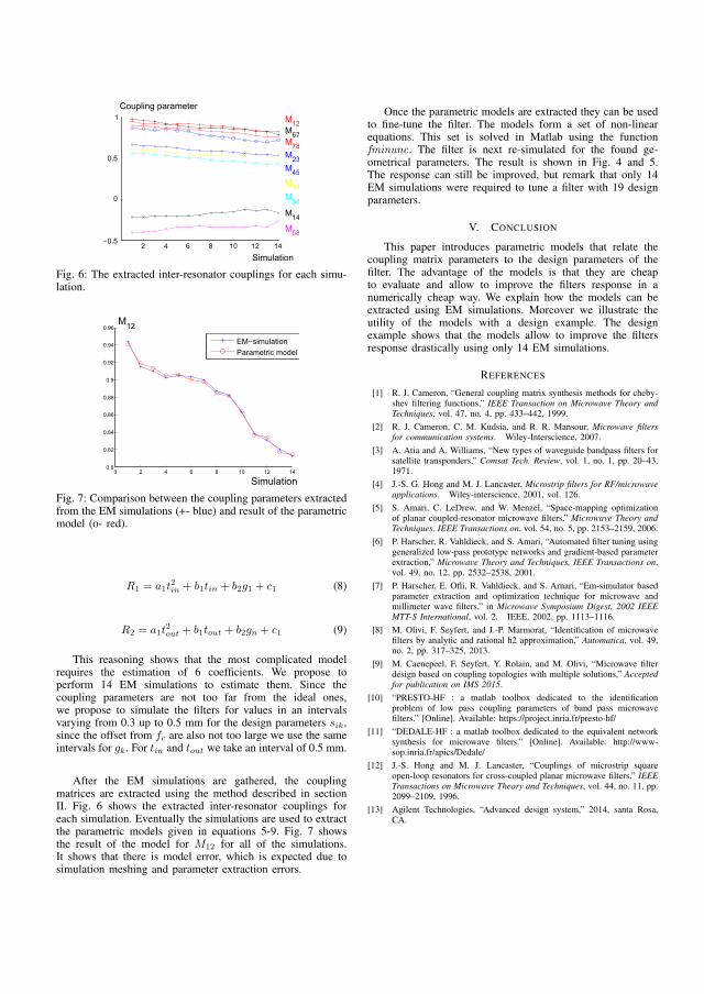
2 4 6 8 10 12 14−0.5

0

0.5

1

Simulation

Coupling parameter

M12

M23

M14

M34

M45

M56

M58

M67

M78

Fig. 6: The extracted inter-resonator couplings for each simu-lation.

0 2 4 6 8 10 12 140.8

0.82

0.84

0.86

0.88

0.9

0.92

0.94

0.96

Simulation

M12

EM−simulation

Parametric model

Fig. 7: Comparison between the coupling parameters extractedfrom the EM simulations (+- blue) and result of the parametricmodel (o- red).

R1 = a1t2in + b1tin + b2g1 + c1 (8)

R2 = a1t2out + b1tout + b2gn + c1 (9)

This reasoning shows that the most complicated modelrequires the estimation of 6 coefficients. We propose toperform 14 EM simulations to estimate them. Since thecoupling parameters are not too far from the ideal ones,we propose to simulate the filters for values in an intervalsvarying from 0.3 up to 0.5 mm for the design parameters sik,since the offset from fc are also not too large we use the sameintervals for gk. For tin and tout we take an interval of 0.5 mm.

After the EM simulations are gathered, the couplingmatrices are extracted using the method described in sectionII. Fig. 6 shows the extracted inter-resonator couplings foreach simulation. Eventually the simulations are used to extractthe parametric models given in equations 5-9. Fig. 7 showsthe result of the model for M12 for all of the simulations.It shows that there is model error, which is expected due tosimulation meshing and parameter extraction errors.

Once the parametric models are extracted they can be usedto fine-tune the filter. The models form a set of non-linearequations. This set is solved in Matlab using the functionfminunc. The filter is next re-simulated for the found ge-ometrical parameters. The result is shown in Fig. 4 and 5.The response can still be improved, but remark that only 14EM simulations were required to tune a filter with 19 designparameters.

V. CONCLUSION

This paper introduces parametric models that relate thecoupling matrix parameters to the design parameters of thefilter. The advantage of the models is that they are cheapto evaluate and allow to improve the filters response in anumerically cheap way. We explain how the models can beextracted using EM simulations. Moreover we illustrate theutility of the models with a design example. The designexample shows that the models allow to improve the filtersresponse drastically using only 14 EM simulations.

REFERENCES

[1] R. J. Cameron, “General coupling matrix synthesis methods for cheby-shev filtering functions,” IEEE Transaction on Microwave Theory andTechniques, vol. 47, no. 4, pp. 433–442, 1999.

[2] R. J. Cameron, C. M. Kudsia, and R. R. Mansour, Microwave filtersfor communication systems. Wiley-Interscience, 2007.

[3] A. Atia and A. Williams, “New types of waveguide bandpass filters forsatellite transponders,” Comsat Tech. Review, vol. 1, no. 1, pp. 20–43,1971.

[4] J.-S. G. Hong and M. J. Lancaster, Microstrip filters for RF/microwaveapplications. Wiley-interscience, 2001, vol. 126.

[5] S. Amari, C. LeDrew, and W. Menzel, “Space-mapping optimizationof planar coupled-resonator microwave filters,” Microwave Theory andTechniques, IEEE Transactions on, vol. 54, no. 5, pp. 2153–2159, 2006.

[6] P. Harscher, R. Vahldieck, and S. Amari, “Automated filter tuning usinggeneralized low-pass prototype networks and gradient-based parameterextraction,” Microwave Theory and Techniques, IEEE Transactions on,vol. 49, no. 12, pp. 2532–2538, 2001.

[7] P. Harscher, E. Ofli, R. Vahldieck, and S. Arnari, “Em-simulator basedparameter extraction and optimization technique for microwave andmillimeter wave filters,” in Microwave Symposium Digest, 2002 IEEEMTT-S International, vol. 2. IEEE, 2002, pp. 1113–1116.

[8] M. Olivi, F. Seyfert, and J.-P. Marmorat, “Identification of microwavefilters by analytic and rational h2 approximation,” Automatica, vol. 49,no. 2, pp. 317–325, 2013.

[9] M. Caenepeel, F. Seyfert, Y. Rolain, and M. Olivi, “Microwave filterdesign based on coupling topologies with multiple solutions,” Acceptedfor publication on IMS 2015.

[10] “PRESTO-HF : a matlab toolbox dedicated to the identificationproblem of low pass coupling parameters of band pass microwavefilters.” [Online]. Available: https://project.inria.fr/presto-hf/

[11] “DEDALE-HF : a matlab toolbox dedicated to the equivalent networksynthesis for microwave filters.” [Online]. Available: http://www-sop.inria.fr/apics/Dedale/

[12] J.-S. Hong and M. J. Lancaster, “Couplings of microstrip squareopen-loop resonators for cross-coupled planar microwave filters,” IEEETransactions on Microwave Theory and Techniques, vol. 44, no. 11, pp.2099–2109, 1996.

[13] Agilent Technologies, “Advanced design system,” 2014, santa Rosa,CA.

Bibliography

[ADS 14] “ADS Momentum”. www.keysight.com, 2014.

[Amar 00a] S. Amari. “Sensitivity analysis of coupled resonator filters”. IEEE

Transactions on Circuits and Systems II: Analog and Digital Signal

Processing, Vol. 47, No. 10, pp. 1017–1022, 2000.

[Amar 00b] S. Amari. “Synthesis of cross-coupled resonator filters using an ana-

lytical gradient-based optimization technique”. IEEE Transactions

on Microwave Theory and Techniques, Vol. 48, No. 9, pp. 1559–

1564, 2000.

[Amar 06] S. Amari, C. LeDrew, and W. Menzel. “Space-mapping optimiza-

tion of planar coupled-resonator microwave filters”. IEEE Trans-

actions on Microwave Theory and Techniques, Vol. 54, No. 5,

pp. 2153–2159, 2006.

[Amar 99] S. Amari. “On the maximum number of finite transmission zeros of

coupled resonator filters with a given topology”. IEEE Microwave

and Guided Wave Letters, Vol. 9, No. 9, pp. 354–356, 1999.

[Ande 73] B. Anderson and S. Vongpanitlerd. Network analysis and synthesis.

NJ, Prentice-Hall, 1973.

[Arnd 04] F. Arndt, J. Brandt, V. Catina, J. Ritter, I. Rullhusen, J. Dauels-

berg, U. Hilgefort, and W. Wessel. “Fast CAD and optimiza-

tion of waveguide components and aperture antennas by hybrid

MM/FE/MoM/FD methods-state-of-the-art and recent advances”.

IEEE Transactions on Microwave Theory and Techniques, Vol. 52,

No. 1, pp. 292–305, 2004.

215

[Atia 71] A. E. Atia and A. E. Williams. “New types of waveguide bandpass

filters for satellite transponders”. Comsat Tech. Review, Vol. 1,

No. 1, pp. 20–43, 1971.

[Atia 72] A. E. Atia and A. E. Williams. “Narrow-bandpass waveguide fil-

ters”. EEE Transactions on Microwave Theory and Techniques,

Vol. 20, No. 4, pp. 258–265, 1972.

[Atia 74] A. E. Atia, A. E. Williams, and R. Newcomb. “Narrow-band

multiple-coupled cavity synthesis”. IEEE Transactions on Circuits

and Systems, Vol. 21, No. 5, pp. 649–655, 1974.

[Atia 98] W. A. Atia, K. A. Zaki, and A. E. Atia. “Synthesis of general

topology multiple coupled resonator filters by optimization”. In:

Microwave Symposium Digest, 1998 IEEE MTT-S International,

pp. 821–824, IEEE, Baltimore, MD, USA, 7-12 June 1998.

[Bahl 77] I. Bahl and R. Garg. “Simple and accurate formulas for a microstrip

with finite strip thickness”. Proceedings of the IEEE, Vol. 65, No. 11,

pp. 1611–1612, 1977.

[Band 88] J. W. Bandler and S. H. Chen. “Circuit optimization: the state of

the art”. IEEE transactions on Microwave Theory and Techniques,

Vol. 36, No. 2, pp. 424–443, 1988.

[Band 94a] J. W. Bandler, R. M. Biernacki, S. H. Chen, D. Swanson, and S. Ye.

“Microstrip filter design using direct EM field simulation”. IEEE

Transactions on Microwave Theory and Techniques, Vol. 42, No. 7,

pp. 1353–1359, 1994.

[Band 94b] J. W. Bandler, R. M. Biernacki, S. H. Chen, D. G. Swanson Jr, and

S. Ye. “Microstrip filter design using direct EM field simulation”.

Microwave Theory and Techniques, IEEE Transactions on, Vol. 42,

No. 7, pp. 1353–1359, 1994.

[Basl 10] P. Basl, R. Gohary, M. Bakr, and R. Mansour. “Modelling of elec-

tromagnetic responses using a robust multi-dimensional Cauchy in-

terpolation technique”. IET Microwaves, Antennas Propagation,,

Vol. 4, No. 11, pp. 1955 –1964, Nov. 2010.

[Bele 68] V. Belevitch. Classical network theory. Holden-Day, 1968.

216

[Bell 82] H. C. Bell Jr. “Canonical asymmetric coupled-resonator filters”.


No. 9, pp. 1335–1340, 1982.

[Belo 75] E. Belohoubek and E. Denlinger. “Loss considerations for microstrip

resonators (short papers)”. IEEE Transactions on Microwave The-

ory and Techniques, Vol. 23, No. 6, pp. 522–526, 1975.

[Ben 03] A. Ben-Israel and T. N. Greville. Generalized inverses: theory and

applications. Vol. 15, Springer Science & Business Media, 2003.

[Bila 99] S. Bila, D. Baillargeat, M. Aubourg, S. Verdeyme, P. Guillon,

C. Zanchi, J. Sombrin, J. Grimm, and L. Baratchart. “Direct

electromagnetic optimisation method for microwave filter design”.

Electronics Letters, Vol. 35, No. 5, pp. 400–401, 1999.

[Broy 65] C. G. Broyden. “A class of methods for solving nonlinear simul-

taneous equations”. Mathematics of Computation, Vol. 19, No. 92,

pp. 577–593, 1965.

[Caen 15a] M. Caenepeel, F. Seyfert, Y. Rolain, and M. Olivi. “Microwave filter

design based on coupling topologies with multiple solutions”. In:

Microwave Symposium (IMS), 2015 IEEE MTT-S International,

pp. 1–4, IEEE, Phoenix, AZ, USA, 17-22 May 2015.

[Caen 15b] M. Caenepeel, F. Seyfert, Y. Rolain, and M. Olivi. “Parametric

modeling of the coupling parameters of planar coupled-resonator

microwave filters”. In: Microwave Conference (EuMC), 2015 Eu-

ropean, pp. 538–541, IEEE, Paris, France, 7-10 Sept 2015.

[Caen 16] M. Caenepeel, K. Chemmangat, F. Ferranti, Y. Rolain, T. Dhaene,

and L. Knockaert. “Scalable macromodelling methodology for the

efficient design of microwave filters”. IET Microwaves, Antennas &

Propagation, Vol. 10, No. 5, pp. 579–586, 2016.

[Came 03] R. J. Cameron. “Advanced coupling matrix synthesis techniques for

microwave filters”. IEEE Transactions on Microwave Theory and

Techniques, Vol. 51, No. 1, pp. 1–10, 2003.

[Came 05] R. J. Cameron, J.-C. Faugere, and F. Seyfert. “Coupling matrix

synthesis for a new class of microwave filter configuration”. In:

Microwave Symposium Digest, 2005 IEEE MTT-S International,

p. 4, Long Beach, CA, USA, 12-17 June 2005.

217

[Came 07a] R. J. Cameron, J.-C. Faugere, F. Rouillier, and F. Seyfert. “Ex-

haustive approach to the coupling matrix synthesis problem and

application to the design of high degree asymmetric filters”. Inter-

national Journal of RF and Microwave Computer-Aided Engineer-

ing, Vol. 17, No. 1, pp. 4–12, 2007.

[Came 07b] R. J. Cameron, C. M. Kudsia, and R. R. Mansour. Microwave filters

for communication systems. Wiley-Interscience, 2007.

[Came 82] R. J. Cameron. “Fast generation of Chebyshev filter prototypes

with asymmetrically-prescribed transmission zeros”. ESA Journal,

Vol. 6, pp. 83–95, 1982.

[Came 99] R. J. Cameron. “General coupling matrix synthesis methods for

Chebyshev filtering functions”. Microwave Theory and Techniques,

IEEE Transactions on, Vol. 47, No. 4, pp. 433–442, 1999.

[Chem 14a] K. Chemmangat, F. Ferranti, T. Dhaene, and L. Knockaert. “Para-

metric macromodelling of linear high-frequency systems using mul-

tiple frequency scaling and sequential sampling”. Electronics Let-

ters, Vol. 50, No. 6, pp. 475–476, 2014.

[Chem 14b] K. Chemmangat, F. Ferranti, T. Dhaene, and L. Knockaert. “Scal-

able models of microwave system responses using sequential sam-

pling on unstructured grids”. International Journal of Numerical

Modelling: Electronic Networks, Devices and Fields, Vol. 27, No. 1,

pp. 122–137, 2014.

[Cohn 58] S. B. Cohn. “Parallel-coupled transmission-line-resonator filters”.

IRE Transactions on Microwave Theory and Techniques, Vol. 6,

No. 2, pp. 223–231, 1958.

[Couc 10] I. Couckuyt, F. Declercq, T. Dhaene, H. Rogier, and L. Knock-

aert. “Surrogate-based infill optimization applied to electromag-

netic problems”. International Journal of RF and Microwave

Computer-Aided Engineering, Vol. 20, No. 5, pp. 492–501, 2010.

[Couc 12] I. Couckuyt, D. Deschrijver, and T. Dhaene. “Towards efficient

multiobjective optimization: multiobjective statistical criterions”.

In: 2012 IEEE Congress on Evolutionary Computation, pp. 1–8,

IEEE, Brisbane, QLD, Australia, 10-15 June 2012.

218

[Cris 72] E. Cristal and S. Frankel. “Hairpin-line and hybrid hairpin-

line/half-wave parallel-coupled-line filters”. IEEE Transactions on

Microwave Theory and Techniques, Vol. 20, No. 11, pp. 719–728,

1972.

[CST 15] “CST Microwave Studio”. www.cst.com, 2015.

[Cuyt 06] A. Cuyt, R. Lenin, S. Becuwe, and B. Verdonk. “Adaptive multi-

variate rational data fitting with applications in electromagnetics”.

IEEE Transactions on Microwave Theory and Techniques,, Vol. 54,

No. 5, pp. 2265 – 2274, May 2006.

[Denl 80] E. J. Denlinger. “Losses of microstrip lines”. IEEE Transactions

on Microwave Theory Techniques, Vol. 28, pp. 513–522, 1980.

[Deva 03] V. Devabhaktuni, B. Chattaraj, M. Yagoub, and Q.-J. Zhang. “Ad-

vanced microwave modeling framework exploiting automatic model

generation, knowledge neural networks, and space mapping”. IEEE

Transactions on Microwave Theory and Techniques,, Vol. 51, No. 7,

pp. 1822 – 1833, July 2003.

[Ferr 09] F. Ferranti, L. Knockaert, and T. Dhaene. “Parameterized S-

Parameter Based Macromodeling With Guaranteed Passivity”.

IEEE Microwave and Wireless Component Letters, Vol. 19, No. 10,

pp. 608–610, Oct. 2009.

[Ferr 10] F. Ferranti, L. Knockaert, and T. Dhaene. “Guaranteed Passive

Parameterized Admittance-Based Macromodeling”. IEEE Trans-

actions on Advanced Packaging, Vol. 33, No. 3, pp. 623–629, Aug.

2010.

[Ferr 11] F. Ferranti, L. Knockaert, and T. Dhaene. “Passivity-Preserving

Parametric Macromodeling by Means of Scaled and Shifted State-

Space Systems”. IEEE Transactions on Microwave Theory and

Techniques, Vol. 59, No. 10, pp. 2394 –2403, Oct. 2011.

[Ferr 12] F. Ferranti, L. Knockaert, T. Dhaene, and G. Antonini. “Parametric

macromodeling based on amplitude and frequency scaled systems

with guaranteed passivity”. International Journal of Numerical

Modelling: Electronic Networks, Devices and Fields, Vol. 25, No. 2,

pp. 139 –151, March/April 2012.

219

[Fook 90] E. H. Fooks and R. A. Zakarevicius. Microwave engineering using

microstrip circuits. Prentice-Hall, Inc., 1990.

[Garc 04] A. Garcıa-Lamperez, S. Llorente-Romano, M. Salazar-Palma, and

T. K. Sarkar. “Efficient electromagnetic optimization of microwave

filters and multiplexers using rational models”. IEEE Transactions

on Microwave Theory and Techniques, Vol. 52, No. 2, pp. 508–521,

2004.

[Garg 79] R. Garg and I. Bahl. “Characteristics of coupled microstriplines”.


No. 7, pp. 700–705, 1979.

[Gilb 63] E. G. Gilbert. “Controllability and observability in multivariable

control systems”. Journal of the Society for Industrial and Applied

Mathematics, Series A: Control, Vol. 1, No. 2, pp. 128–151, 1963.

[Gopi 81] A. Gopinath. “Maximum Q-factor of microstrip resonators”. IEEE


pp. 128–131, 1981.

[Gupt 79] K. Gupta, R. Garg, I. Bahl, and P. Bhartia. Microstrip lines and

slotlines. Vol. 2, Artech house Dedham, Massachusetts, 1979.

[Gust 06] B. Gustavsen. “Improving the pole relocating properties of vector

fitting”. IEEE Transactions on Power Delivery, Vol. 21, No. 3,

pp. 1587–1592, July 2006.

[Gust 99] B. Gustavsen and A. Semlyen. “Rational approximation of fre-

quency domain responses by Vector Fitting”. IEEE Transactions

on Power Delivery, Vol. 14, No. 3, pp. 1052–1061, July 1999.

[Hamm 80] E. Hammerstad and O. Jensen. “Accurate models for microstrip

computer-aided design”. In: 1980 IEEE MTT-S International Mi-

crowave Symposium Digest, pp. 407–409, Washington, DC, USA,

28-30 May 1980.

[Harr 96] R. F. Harrington and J. L. Harrington. Field computation by mo-

ment methods. Oxford University Press, 1996.

[Hars 01] P. Harscher, R. Vahldieck, and S. Amari. “Automated filter tuning

using generalized low-pass prototype networks and gradient-based

parameter extraction”. IEEE Transactions on Microwave Theory

and Techniques, Vol. 49, No. 12, pp. 2532–2538, 2001.

220

[Hars 02] P. Harscher, E. Ofli, R. Vahldieck, and S. Arnari. “EM-simulator

based parameter extraction and optimization technique for mi-

crowave and millimeter wave filters”. In: Microwave Symposium

Digest, 2002 IEEE MTT-S International, pp. 1113–1116, IEEE,

Seattle, WA, USA, 2-7 June 2002.

[Hong 00] J.-S. Hong. “Couplings of asynchronously tuned coupled microwave

resonators”. IEE Proceedings: Microwaves, Antennas and Propa-

gation, Vol. 147, No. 5, pp. 354–358, 2000.

[Hong 01] J.-S. Hong and M. J. Lancaster. Microstrip filters for RF/microwave

applications. Vol. 126, Wiley-interscience, 2001.

[Hong 96] J.-S. Hong and M. J. Lancaster. “Couplings of microstrip square

open-loop resonators for cross-coupled planar microwave filters”.


No. 11, pp. 2099–2109, 1996.

[Hong 99] J.-S. Hong and M. Lancaster. “Microstrip cross-coupled trisec-

tion bandpass filters with asymmetric frequency characteristics”.

IEE Proceedings: Microwaves, Antennas and Propagation, Vol. 146,

No. 1, pp. 84–90, 1999.

[Hsu 13] C.-Y. Hsu, C.-Y. Chen, and H.-R. Chuang. “Microstrip dual-band

bandpass filter design with closely specified passbands”. Microwave

Theory and Techniques, IEEE Transactions on, Vol. 61, No. 1,

pp. 98–106, 2013.

[Hu 13] H. Hu and K.-L. Wu. “An adaptive computer-aided design-and-

tuning scheme for a predistorted filter with uneven-Q effect”. In:

Microwave Symposium Digest (IMS), 2013 IEEE MTT-S Interna-

tional, pp. 1–3, IEEE, Seattle, WA, USA, 2-7 June 2013.

[Hu 14] H. Hu and K.-L. Wu. “A Generalized Coupling Matrix Extraction

Technique for Bandpass Filters With Uneven-Qs”. IEEE Transac-

tions on Microwave Theory and Techniques, Vol. 62, No. 2, pp. 244–

251, Feb 2014.

[Kail 80] T. Kailath. Linear systems. Vol. 156, Prentice-Hall Englewood

Cliffs, NJ, 1980.

[Kirs 84] M. Kirschning and R. H. Jansen. “Accurate wide-range design equa-

tions for the frequency-dependent characteristic of parallel coupled

221

microstrip lines”. IEEE Transactions on Microwave Theory and

Techniques, Vol. 32, No. 1, pp. 83–90, 1984.

[Klei 08] J. P. C. Kleijnen. Design and Analysis of Simulation Experiments.

Springer, 2008.

[Klim 05] A. Klimke and B. Wohlmuth. “Algorithm 847: spinterp: Piecewise

Multilinear Hierarchical Sparse Grid Interpolation in MATLAB”.

ACM Transactions on Mathematical Software, Vol. 31, No. 4, 2005.

[Klim 07] A. Klimke. “Sparse Grid Interpolation Toolbox – User’s Guide”.

Tech. Rep. IANS report 2007/017, University of Stuttgart, 2007.

[Koza 02] P. Kozakowski and M. Mrozowski. “Automated CAD of coupled

resonator filters”. IEEE Microwave and Wireless Components Let-

ters, Vol. 12, No. 12, pp. 470–472, 2002.

[Koza 06] P. Kozakowski and M. Mrozowski. “Quadratic programming ap-

proach to coupled resonator filter CAD”. IEEE Transactions on

Microwave Theory and Techniques, Vol. 54, No. 11, pp. 3906–3913,

2006.

[Kozi 06] S. Koziel, J. Bandler, and K. Madsen. “A Space-Mapping Frame-

work for Engineering Optimization; Theory and Implementation”.

IEEE Transactions on Microwave Theory and Techniques,, Vol. 54,

No. 10, pp. 3721 –3730, Oct. 2006.

[Kozi 10a] S. Koziel. “Shape-Preserving Response Prediction for Microwave

Design Optimization”. IEEE Transactions on Microwave Theory

and Techniques,, Vol. 58, No. 11, pp. 2829 –2837, Nov. 2010.

[Kozi 10b] S. Koziel, J. Bandler, and Q. Cheng. “Robust Trust-Region Space-

Mapping Algorithms for Microwave Design Optimization”. IEEE

Transactions on Microwave Theory and Techniques,, Vol. 58, No. 8,

pp. 2166 –2174, Aug. 2010.

[Kuds 92] C. Kudsia, R. Cameron, and T. Wai-Cheung. “Innovations in mi-

crowave filters and multiplexing networks for communications satel-

lite systems”. IEEE Transactions on Microwave Theory and Tech-

niques, Vol. 40, No. 6, pp. 1133–1149, 1992.

[Kuro 65] K. Kurokawa. “Power waves and the scattering matrix”. IEEE


pp. 194–202, 1965.

222

[Lame 03] A. Lamecki, P. Kozakowski, and M. Mrozowski. “Efficient imple-

mentation of the Cauchy method for automated CAD-model con-

struction”. IEEE Microwave and Wireless Components Letters,,

Vol. 13, No. 7, pp. 268 –270, July 2003.

[Lame 09] A. Lamecki, L. Balewski, and M. Mrozowski. “Adaptive CAD-

Model Construction Schemes”. IEEE Transactions on Magnetics,,

Vol. 45, No. 3, pp. 1538 –1541, March 2009.

[Lamp 04] A. G. Lamperez, T. K. Sarkar, and M. S. Palma. “Generation of ac-

curate rational models of lossy systems using the Cauchy method”.

IEEE Microwave and Wireless Components Letters, Vol. 14, No. 10,

pp. 490–492, 2004.

[Lehm 01] R. Lehmensiek and P. Meyer. “Creating accurate multivariate ra-

tional interpolation models of microwave circuits by using efficient

adaptive sampling to minimize the number of computational elec-

tromagnetic analyses”. IEEE Transactions on Microwave Theory

and Techniques, Vol. 49, No. 8, pp. 1419 –1430, Aug. 2001.

[Levy 02] R. Levy, R. V. Snyder, and G. Matthaei. “Design of microwave

filters”. IEEE Transactions on Microwave Theory and Techniques,

Vol. 50, No. 3, pp. 783–793, 2002.

[Levy 84] R. Levy and S. B. Cohn. “A history of microwave filter research, de-

sign, and development”. IEEE Transactions on Microwave Theory

and Techniques, Vol. 32, No. 9, pp. 1055–1067, 1984.

[Macc 08] G. Macchiarella. “Generalized coupling coefficient for filters with

nonresonant nodes”. IEEE Microwave and Wireless Components

Letters, Vol. 18, No. 12, pp. 773–775, 2008.

[Macc 10] G. Macchiarella. “Extraction of unloaded Q and coupling matrix

from measurements on filters with large losses”. Microwave and

Wireless Components Letters, IEEE, Vol. 20, No. 6, pp. 307–309,

2010.

[Mark 92] R. B. Marks and D. F. Williams. “A general waveguide circuit

theory”. Journal of Research-National Institute of Standards and

Technology, Vol. 97, pp. 533–533, 1992.

[Marm 02] J.-P. Marmorat, M. Olivi, B. Hanzon, and R. L. Peeters. “Matrix

rational H 2 approximation: a state-space approach using Schur

223

parameters”. In: Proceedings of the 41st IEEE Conference on Deci-

sion and Control, pp. 4244–4249, IEEE, Las Vegas, NV, USA, 10-13

Dec. 2002.

[Mart 12] M. Martinez-Mendoza, F. Seyfert, C. Ernst, and A. Alvarez-Melcon.

“Formal Expression of Sensitivity and Energy Relationship in the

Context of the Coupling Matrix”. IEEE Transactions on Microwave

Theory and Techniques, Vol. 60, No. 11, pp. 3369–3375, 2012.

[Matt 64] G. L. Matthaei, L. Young, and E. Jones. Microwave filters,

impedance-matching networks, and coupling structures. Vol. 5,

McGraw-Hill New York, 1964.

[Mira 08] V. Miraftab and M. Yu. “Generalized lossy microwave filter cou-

pling matrix synthesis and design using mixed technologies”. IEEE


pp. 3016–3027, 2008.

[Mont 48] C. G. Montgomery, R. H. Dicke, and E. M. Purcell. Principles of

microwave circuits. Iet, 1948.

[Oliv 13] M. Olivi, F. Seyfert, and J.-P. Marmorat. “Identification of mi-

crowave filters by analytic and rational H2 approximation”. Auto-

matica, Vol. 49, No. 2, pp. 317–325, 2013.

[Part 97] J. R. Partington. Interpolation, identification, and sampling. Ox-

ford University Press, 1997.

[Peik 98] S. Peik, R. Mansour, and Y. Chow. “Multidimensional Cauchy

method and adaptive sampling for an accurate microwave circuit

modeling”. IEEE Transactions on Microwave Theory and Tech-

niques,, Vol. 46, No. 12, pp. 2364 –2371, Dec. 1998.

[Pint 12] R. Pintelon and J. Schoukens. System Identification: A Frequency

Domain Approach. Wiley-IEEE Press, 2012.

[Poza 98] D. Pozar. Microwave engineering. John Wiley & Sons, 1998.

[Puce 68] R. A. Pucel, D. J. Masse, and C. P. Hartwig. “Losses in microstrip”.


No. 6, pp. 342–350, 1968.

224

[Pugl 00] K. Puglia. “A General Design Procedure for Bandpass Filters De-

rived from Lowpass Prototype Elements: Part I”. Microwave Jour-

nal -Euroglobal Edition-, Vol. 43, No. 12, pp. 22–38, 2000.

[Pugl 01] K. Puglia. “A general design procedure for bandpass filters derived

from low pass prototype elements: Part II”. Microwave Journal

-Euroglobal Edition-, Vol. 44, No. 1, pp. 114–137, 2001.

[RARL] “RARL2: a Matlab toolbox dedicated to the computa-

tion of a stable rational L2-approximation of specified order

to a given L2-stable matrix-valued function”. http://www-

sop.inria.fr/apics/RARL2/rarl2.html.

[Seyf 00] F. Seyfert. “DEDALE-HF: a Matlab toolbox dedicated to the

equivalent network synthesis for microwave filters”. http://www-

sop.inria.fr/apics/Dedale/, 2000.

[Seyf 03] F. Seyfert, L. Baratchart, J.-P. Marmorat, S. Bila, J. Sombrin, et

al. “Extraction of coupling parameters for microwave filters: De-

termination of a stable rational model from scattering data”. In:

IEEE MTT-S International Microwave Symposium Digest, pp. 25–

30, Citeseer, 2003.

[Seyf 04] F. Seyfert. “PRESTO-HF: a Matlab toolbox dedicated to the iden-

tification problem of low pass coupling parameters of band pass

microwave filters”. https://project.inria.fr/presto-hf/, 2004.

[Seyf 07] F. Seyfert and S. Bila. “General synthesis techniques for coupled

resonator networks”. IEEE Microwave Magazine, Vol. 8, No. 5,

pp. 98–104, Oct 2007.

[Seyf 98] F. Seyfert. Problemes extremaux dans les espaces de Hardy. PhD

thesis, Ecole Nationale Superieure des Mines de Paris, 1998.

[Snyd 07] R. V. Snyder. “Practical aspects of microwave filter development”.

IEEE Microwave Magazine, Vol. 8, No. 2, pp. 42–54, 2007.

[Swan 07a] D. Swanson and G. Macchiarella. “Microwave filter design by syn-

thesis and optimization”. IEEE Microwave Magazine, Vol. 8, No. 2,

pp. 55–69, 2007.

[Swan 07b] D. Swanson. “Narrow-band microwave filter design”. IEEE Mi-

crowave Magazine, Vol. 8, No. 5, pp. 105–114, 2007.

225

[Tami 05] S. Tamiazzo and G. Macchiarella. “An analytical technique for the

synthesis of cascaded N-tuplets cross-coupled resonators microwave

filters using matrix rotations”. IEEE Transactions on Microwave

Theory and Techniques, Vol. 53, No. 5, pp. 1693–1698, 2005.

[Triv 09] P. Triverio, S. Grivet-Talocia, and M. Nakhla. “A Parameter-

ized Macromodeling Strategy With Uniform Stability Test”. IEEE

Transactions on Advanced Packaging, Vol. 32, No. 1, pp. 205 –215,

Feb. 2009.

[Triv 10] P. Triverio, M. Nakhla, and S. Grivet-Talocia. “Passive parametric

macromodeling from sampled frequency data”. In: 2010 IEEE 14th

Workshop on Signal Propagation on Interconnects (SPI), pp. 117–

120, IEEE, Hildesheim, The Netherlands, 9-12 May 2010.

[Wang 07] G. G. Wang and S. Shan. “Review of Metamodeling Techniques in

Support of Engineering Design Optimization”. Journal of Mechan-

ical Design, Vol. 129, No. 4, pp. 370–380, 2007.

[Wong 79] J. S. Wong. “Microstrip tapped-line filter design”. IEEE Transac-

tions on Microwave Theory Techniques, Vol. 27, pp. 44–50, 1979.

[Yang 99] C.-C. Yang and C.-Y. Chang. “Microstrip cascade trisection filter”.

IEEE Microwave and Guided Wave Letters, Vol. 9, No. 7, pp. 271–

273, 1999.

226

modeling technique for the efficient design of microwave

Documents