1 | K u h n

Modeling rainfall-runoff using SWAT in a

small urban wetland Tests of scale for the Soil and Water Assessment Tool hydrology model

Catherine Kuhn

FES 724 Watershed Cycles and Processes | Spring 2014

Yale University School of Forestry and Environmental Studies

2 | K u h n

Abstract

Understanding urban wetland functions from an ecosytem services framework allows

managers to base restoration efforts on multiple user end-benefits. Wetlands can provide the

coupled function of improving water quality and mitigating floods through delayed stormwater

flow. The Yale Environmental Watershed, a 5.1 hectare forested wetland located in New Haven,

CT, has been identified as a potential asset for improving stormwater management and

mitigating flooding on the Yale University campus and adjacent properties. The wetland

currently only drains 46% of its watershed with the balance of its area flowing into an

overburdened sewage infrastructure. The general aim of this project was to develop a

hydrologic model characterizing the watershed’s water balance to inform restoration efforts.

The Soil and Water Assessment Tool (SWAT) was chosen to test its applicability in small, urban

watersheds. Using this model, simulated hydrographs were assessed for accuracy over a two-

year period. Data from March 2013-April 2014 were used to evaluate the model performance.

The model achieved a reasonable fit after calibration with a Nash Sutcliffe Efficiency Index of

0.59. Hoever, the model was insensitive to seasonal water budget drivers such as

evapotranspiration and snowmelt. This work provides a case study for simulating hydrologic

processes on small-scale, urban, partially developed wetlands and is part of the evolving

endeavor to adapt SWAT modeling tools to urban landscapes.

KEY WORDS: SWAT MODEL, STORM WATER, URBAN, WETLAND

Introduction

As population density and development continue trending upward, stormwater runoff from

increased impervious surfaces presents challenges on local and global scales (Assessment

2005). Besides collecting contaminants from urban surfaces (nutrients, road salt, heavy metals,

pesticides and bacteria), changes in storm water flow patterns can cause stream degradation,

erosion, flooding and accompanying property damage (Sartor, Boyd et al. 1974). Understanding

urban flow patterns on finer scales is a critical first step to effective water management and

flood hazard mitigation.

These flow patterns can then be used to select best management practices for stormwater

management. Such management practices include rerouting impervious surface flow out of

sewage infrastructure. Another approach is increasing infiltration and recharge through the use

of wetlands or bioswales. Hydrological watershed modeling has become a central tool for

conceptualizing these flows of surface and subsurface water. Models can then be used to

generating decision support tools for policy makers, regulators and resource managers (Daniel,

Camp et al. 2011). Besides establishing water balances, models can also be used to predict the

3 | K u h n

impact of different management practices on rainfall-runoff response, sediment and

contaminant transport (Elliott and Trowsdale 2007).

The SWAT model, initially developed in the 1980s for managing water supplies and non-point

source pollution in agricultural river basins (Arnold, Srinivasan et al. 1998, Daniel, Camp et al.

2011, Tuppad, Douglas-Mankin et al. 2011), is increasingly being applied to extended settings

including urban watersheds (Easton, Fuka et al. 2008). A physically-based, non-proprietary,

semi-distributed model, SWAT is computationally efficient and relies on readily-available data

to simulate upland and channel processes. The model can operate on a daily, monthly or annual

timestep and has historically been used to develop TDMLs. These characteristics, along with the

model’s capacity to quantify sediment, nutrient and bacteria loading based on different land

management scenarios, make SWAT a strong candidate for use in urban watersheds as a water

quality model.

This study seeks to apply this widely used model in the novel context of a small urban

watershed to test the model’s ability perform on fine spatio-temporal scales. Urban stream

restoration sites often occupy small acreage and have limited access to onsite observed data

records of any significant time span. If SWAT, a free and widely available model, can be used to

simulate discharge and pollutant loading on this small scale, then the model outputs can be

used to identify potential impacts of restoration efforts.

THE RESEARCH CATCHMENT

The Yale swale, a 5-acre partially undeveloped land

parcel located by the Yale University School of

Forestry (Figure 1), represents a unique testing

ground for analysis of hydrologic models and

improved water management on a micro-urban

scale. Unpublished work by prior research assistants

suggests this small part of a larger ~20 acre

watershed could hold potential value for improving

campus storm water management for runoff

generated by the 636.783 square feet of impervious

surface area within the swale (Khadka 2013). Based

on these preliminary studies, the 2013 Yale

Sustainable Stormwater Management Plan

identified the swale as a potential site for green

infrastructure intervention. The assessment

suggested re-routing the neighboring downspouts Figure 1 Location of the Yale

Experimental Watershed

4 | K u h n

into the wetland instead of into the sewage system could help reduce sewage overflows during

storm events. Best management practices can be used to mitigate storm water problems such

as pollutant transport, high peak flows and extreme flow volumes (Hunt, Kannan et al. 2009).

However, any proposed conservation scenarios require an accurate understanding of flow

patterns in the swale, which has historically been limited by a lack of continuous local data.

As of April 2013, however, calculations of a basic

water budget are now possible due to the

installation of two V-notch weirs (Figure 2), a

radiometer, a tipping bucket and groundwater wells.

This study seeks to create a hydrologic model

calibrated with this observed data.

GOALS AND OBJECTIVES

The goals of this research proposal are to test and

evaluate the applicability of the ArcSWAT model

under the hydrologic, urbanized, and climactic

conditions of a small urban watershed in Connecticut. This proposal seeks to address the

following question: How does applying SWAT to a small urban watershed impact its predictive

performance? Testing the robustness of SWAT in such a small basin will contribute more

understanding of model performance in a relatively understudied context.

The objective of this research plan is to generate and calibrate a hydrologic model of the Swale

watershed. The outcome will be a complete hydrologic model that could be used to inform

management and research efforts conducted by Yale facilities, faculty and students. This

baseline will provide estimates of peak flow and surface run-off that can be used to inform

adjacent landowners and Yale facilities of potential hazards from flooding as well as

opportunities to improve water resource management.

Methods

The following sections describe the framework and assumptions of the SWAT model as well as

model inputs and outputs. The final sections describe model calibration and analysis of output

data.

SWAT THEORETICAL FRAMEWORK

The Soil and Water Assessment Tool (SWAT) is a deterministic, continuous watershed model

that can operate on daily and hourly time steps (Daniel, Camp et al. 2011). This project will use

ArcSWAT 2012.10.13 to generate a hydrologic model of the Yale Swale watershed in a GIS user

interface. ArcSWAT allows the conversion of raster and vector data into model outputs. A 2-

Figure 2 V-notch weir at inlet of study site, 2013

5 | K u h n

year simulation period from 2013-2014 will be used, which coincides with the year of available

field discharge data. The model relies on governing equations to control the movement of

water through surface, subsurface and lateral flow in each subbasin (Borah and Bera 2003). The

following equations are targeted because of their relevance to the study’s objective and goals.

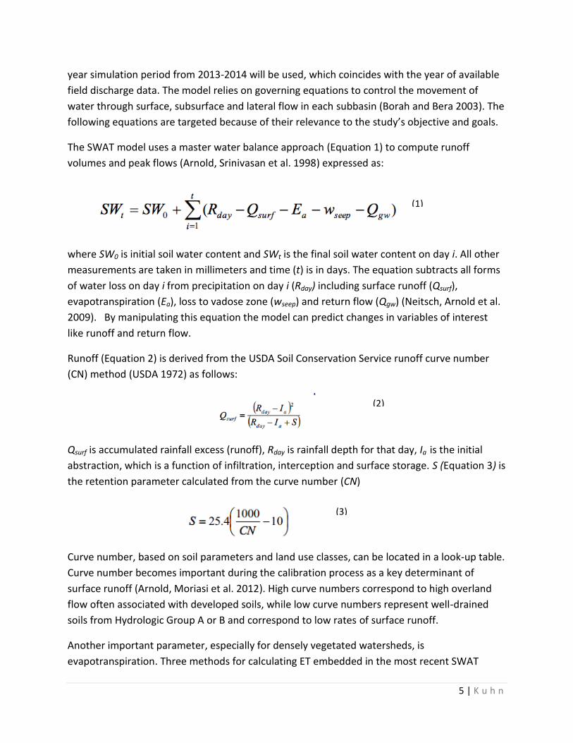
The SWAT model uses a master water balance approach (Equation 1) to compute runoff

volumes and peak flows (Arnold, Srinivasan et al. 1998) expressed as:

where SW0 is initial soil water content and SWt is the final soil water content on day i. All other

measurements are taken in millimeters and time (t) is in days. The equation subtracts all forms

of water loss on day i from precipitation on day i (Rday) including surface runoff (Qsurf),

evapotranspiration (Ea), loss to vadose zone (wseep) and return flow (Qgw) (Neitsch, Arnold et al.

2009). By manipulating this equation the model can predict changes in variables of interest

like runoff and return flow.

Runoff (Equation 2) is derived from the USDA Soil Conservation Service runoff curve number

(CN) method (USDA 1972) as follows:

Qsurf is accumulated rainfall excess (runoff), Rday is rainfall depth for that day, Ia is the initial

abstraction, which is a function of infiltration, interception and surface storage. S (Equation 3) is

the retention parameter calculated from the curve number (CN)

Curve number, based on soil parameters and land use classes, can be located in a look-up table.

Curve number becomes important during the calibration process as a key determinant of

surface runoff (Arnold, Moriasi et al. 2012). High curve numbers correspond to high overland

flow often associated with developed soils, while low curve numbers represent well-drained

soils from Hydrologic Group A or B and correspond to low rates of surface runoff.

Another important parameter, especially for densely vegetated watersheds, is

evapotranspiration. Three methods for calculating ET embedded in the most recent SWAT

(1)

(2)

(3)

6 | K u h n

model include the Penman-Monteith, Priestley-Taylor, and Hargreaves. Hargreaves is the

simplest appraoch requiring only air temperature. The other two approaches require solar

radiation, air temperature and relative humidity, with Penman-Monteith adding wind speed as

well (Neitsch, Arnold et al. 2009). Recent research has shown that modeled Penman Monteith

ET rates have held up well against empirical calculations (Earls and Dixon 2008). The Penman-

Monteith equation will be used for this study.

Subsurface flow will be an important parameter for this wetland because lateral flow can

decrease system flashiness in urban areas and provide reduced-cost ecosystem services such as

improved water quality (Neralla, Weaver et al. 2000). The equation for lateral flow is derived

from a series of inputs regarding hillslope, soil porosity, field capacity, hydraulic conductivity

and volume of soil water (Neitsch, Arnold et al. 2009).

Flow routing, another important set of governing equation, contributes to flow speed and

direction. The velocity and rate of flow are defined by Manning’s equation, which uses rate of

flow, slope, a roughness coefficient and a hydraulic radius (cross section of flow). SWAT has two

routing methods: variable and Muskingum routing that model storage volume and routing

patterns (Neitsch, Arnold et al. 2009). These equations are used to route water over HRU

topography into stream reaches and main channels and can be important in outputs where a

lag in surface runoff could indicate overestimation of surface roughness.

The goal of this study is to parameterize the model, especially for the curve number term, in

order to achieve surface runoff values comparable to observed records. This runoff can then be

used to develop the rest of the water budget. The governing equations described above use

information about rainfall, watershed area, soil permeability, land use and soil water conditions

to predict peak runoff (Sultan).

ASSUMPTIONS AND DRAWBACKS

While the SWAT model has been empirically considered as a robust and flexible model, several

studies demonstrate the drawbacks of this model (Daniel, Camp et al. 2011). Gassman, et al

demonstrated that the model’s HRU units lack the ability to accurately represent parceled land

units like riparian zones and wetlands or targeted management interventions (Gassman 2007).

The model also fares poorly at predicting individual flood events because it operates on a

continuous daily time step instead of being event-based (Borah and Bera 2003). In addition,

the curve-number model used to calculate run-off implies assumptions about soil parameters

that are not true for all regions. The empirically-derived CN method is based on infiltration-

excess model, which is inappropriate for watersheds where rainfall runoff from rain in excess of

the saturated conductivity rarely occurs (Gassman 2007). A 2011 paper replaced the curve

number method with a physically-based water balance yielding the same or more accurate

results for the Catskills (White, Easton et al. 2011).

7 | K u h n

MODEL CONFIGURATION

To run SWAT, Macintosh computers require a partitioned hard drive with a Windows side. This

partition can be created with the program Bootcamp, which is also required run ArcMap 10.1 as

a platform for ArcSWAT 2012.10.14. The SWAT program itself can be downloaded for free from

http://swat.tamu.edu/software/arcswat/. The model follows a basic workflow pattern

described by Figure 3.

Figure 3 SWAT Model Process

DATA PRE-PROCESSING

The SWAT model requires input parameters including a digital elevation model for contour and

slope, climate, soil characteristics and land cover (Srinivasan , Arnold 2012). Additional

information about water infrastructure and land management practices can also be

incorporated. Each parameter is listed below and can be obtained from open-access, free public

databases at varying resolutions. Many inputs are contained within the model, sometimes on a

coarse scale. Inputs derived from local measurements may require a larger degree of pre-

processing. All input files were pre-processed through re-projection and resampling into the

Connecticut State Plane Projection 0600 with a 10 foot resolution.

8 | K u h n

WATERSHED DELINEATION

The first step in model construction is the

delineation of the watershed and its

associated sub-basins and reaches. As a

physically based model, SWAT derives

topography, contour and slope from a digital

elevation model used to divide the basin into

sub-watersheds (Zhou and Fulcher 1997). Sub-

basin boundaries are created using the Arc

Map watershed delineation toolkit and can be

manipulated based on observed routing

patterns, soil types and land uses. The

watershed (Figure 4) was delineated using a

global digital elevation model (DEM) from the

University of Connecticut’s Center for Land

Use Education and Research (CLEAR). This

DEM, generated by the airborne Lidar readings

taken in 2000, has 10 ft spatial resolution and

uses the North American Datum (NAD) Connecticut State Plane Coordinate System Zone 0600

with a Lambert Conformal Conic projection. The GDEM covers the entire quadrangle of New

Haven and was clipped using a basin mask manually generated in SWAT for faster data

processing.

This DEM file, the base topographic input into the ArcSWAT model, is used to calculate the

slope and contours of the watershed. Once the DEM is added, the model then uses the

contours and watershed slope, calculated during the delineation, to determine flow direction

and accumulation. Once flow direction and accumulation have been established, the model

generates a stream network in which each individual reach drains a subbasin, all of which drain

into a major reach. Each reach has a node or outlet. The modeler then selects a node that

corresponds to the outlet at which the discharge measurements for calibration are being

collected. This outlet sets the lower bound for the watershed basin, which is then delineated

based on the location of that outlet and the stream network. Recorded GPS points from the

swale were uploaded to the ArcMap data manager and used as guidance during the selection of

the watershed outlet.

HRU ANALYSIS

In order to define Hydrologic Response Units (HRUs), the model requires data on land use, soil

type and slope. Watershed slope is derived from the digital elevation model using the Slope

Spatial Analysis tool in ARC Map 10.1. Using the DEM file as the input raster, the tool translates

the elevation into a slope projection using percent slope. This parameter will be used in SWAT

Figure 4 Initial Watershed Delineation

9 | K u h n

Figure 5 Land Cover Classification from 2006 Thematic Mapper

Table 1 Land Cover Classes by Model Run

to fill in the subsurface lateral water

movement, flow accumulation and routing as

well as sediment yield for each subbasin

(Arnold, Srinivasan et al. 1998). The results of

this preprocessing step (Figure 3) create finer

scale variability in slope characteristics within

our current study area.

Land use data can be obtained for free from

the National Land Cover Database at 100 ft

resolution in the NAD 1983 Connecticut State

Plane Projection. The three land use classes in

the 2006 land cover classification from the

NLCD (Figure 5) identify the swale as

containing deciduous forest (green), medium

density residential development (red) and turf

grass (yellow). The SWAT model associates

each land cover type with a cluster of

parameter values include those related to lateral

flow, ET and overland flow. This land use classification is clearly problematic. The rationale for

its use was to set a lower bound for model performance using the most readily available data

layers in order to observe output hydrograph accuracy developed using the most generic

approach.

After initial calibration the 2006 NLCD layer was validated with a secondary data set quantifying

percent imperviousness. This 2011 data layer, also available from the NLCD, was downloaded

and clipped to the basin size. Zonal statistics were

used to identify the average percent impervious area

for the basin. The results showed average

imperviousness for the basin as 16%, in contrast to

the 57% urban cover shown in the original 2006

NLCD layer. A 2008 orthophotograph of the site was

also projected underneath the 2006 NLCD layer

(Appendix A) clearly highlighting incorrectly classified pixels. For the second model run, land

cover classes were changed to reflect this more accurate result (Table 1).

Soil type is a third required input to the SWAT model. The Soil Conservation Service (SCS) of the

United States Department of Agricultural has three digital soil databases at different levels of

intensities. The standardized soil layer used by SWAT is STATSGO, a coarse resolution model

10 | K u h n

(250km) featuring only one soil class for our study site. SSURGO, a second data set produced by

SCS, has finer spatial resolution and has been shown to produce more accurate outputs in

irrigation dominated watersheds (Wang and Melesse 2006). SSURGO data, however, has a large

file size and requires another series of pre-processing before it is usable. For the purposes of

this study, the basic STATSGO data was used as inputs to set the lower bounds of model input

data specificity.

Both databases can downloaded for free from the Connecticut Department of Energy &

Environmental Protection’s Soil Survey Geographic and provide information on soil location,

distribution and classifications (USDA-NRCS 2007). The soil map unit key column of the attribute

table contains a unique identifier indicating soil type, which the SWAT model will use to collect

information about hydraulic conductivity and other soil properties influencing hydrologic

processes. The STATSGO file was pre-processed using a nearest neighbor resampling and raster

reprojection to correspond to the other input files. As a result of the coarse resolution, the soil

class map shows only one soil type (sandy loam) for the entire study site. This can clearly be

refined by field samples.

Once these land use, soil type and slope were defined, hydrologic response units (HRUs), were

created with unique combinations of those classes. Each HRU features class-specific parameters

that can be manually adjusted.

The final step before simulation was the creation of input tables, including

weather information. Climate data, generated by the model or input from read records, is

used in tandem with geographic data sets to generate hydrologic flow patterns in the subbasin.

Long term data on temperature and precipitation was obtained from NOAA National Climactic

Data Center database in a daily time step for Tweed airport (USGS-NWIS 2014). Precipitation on

site has been recorded using a Rainwise tipping bucket, which has been collecting 15 and 5

minute time step readings since last October. The SWAT model has a built in weather generator

that can be used to fill gaps in data. This generator, called WXGEN, predicts daily weather

variables for specific geographic locations. The first model run was based on WXGEN

automatically generated weather data. The second model run incorporated observed

precipitation and temperature data from the onsite tipping bucket and Tweed airport. WXGEN

input files from the NOAA records were built for the 2 year period of rainfall from 2013-2013

that matched the window of observed streamflow data in addition to several months of model

warm up time.

OUTPUTS

Useful model outputs are ET, surface runoff, peak flow, sediment loading, nutrient loading,

ground water movement (infiltrated water going to aquifer), soil water content, lateral

11 | K u h n

(subsurface) flow, infiltration (Srinivasan, Ramanarayanan et al. 1998). For the scope of this

project, analysis focused on the discharge hydrographs created during model runs.

CALIBRATION & STATISTICAL ANALYSIS

The Soil and Water Assessment model has been broadly applied because of flexible

parameterization. With very few required inputs, the model can be ran almost entirely on data

that is widely available and free –an asset for researchers working in un-gauged basins with

limited access to data on finer spatial scales. Model outputs, however, are only as accurate as

the input data and governing equations. Therefore, model calibration is necessary to ground

results in field-tested data if at all possible.

The first step of calibration was to conduct a sensitivity analysis identifying which parameters

most heavily weight the rates of change in the model. This step establishes which processes

dominate hydrologic activity in the model (Arnold, Moriasi et al. 2012). After the sensitivity

analysis, the model was calibrated using stream discharge data from the v-notch weir in the

swale. Using model outputs, a Nash Sutcliffe efficiency (NSE) statistical index (Equation 4) was

generated to assess the accuracy of the model.

This index, in addition to r2, is the most widely used method for model calibration and validation

(Arnold, Moriasi et al. 2012). An NSE of zero or less indicates the simulation is not able to

predict discharge while an NSE of 1 indicates the model’s performance falls within an

acceptable range of uncertainty. Moriasi, et al argues NSE values of 0.54-0.65 are adequate and

any values greater than 0.5 are satisfactory (Moriasi, Arnold et al. 2007).

Results

INITIAL MODEL RESULTS

For the preliminary model run

(Appendix B, Model A), the WGEN

weather generator was used to

simulate climate conditions. The

model outputs, therefore, cannot

be used for calibration. Instead,

the predicted discharge can be

used to give a general idea of the

(4)

Figure 6 Stream Discharge from Model A (Simulated Weather)

12 | K u h n

Figure 7 Simulated and Observed Discharge for Model B

model performance. Using simulated weather, the model under predicted evaporation (Figure

7) as only composing 13% of precipitation, a ratio unlikely here in New England. In addition, the

model generated a curve number of 71.64. Curve numbers in the 70s are associated with

developed urban areas. On the ground examinations of the field site and current satellite

photos show that most of the study site is actually deciduous forest. Therefore, the curve

number in this initial model was artificially inflated by the misclassified land use raster layer.

Clear problems in the model’s ability to predict physical processes indicate that SCS runoff

curve number and parameters governing evapotranspiration should be adjusted in the

calibration process.

UNCALIBRATED MODEL RESULTS

The second model run (Appendix B, Model B) incorporated both observed weather data and

improved land use classification. Changing the land cover classification (60% forested instead of

urban) generated a slightly more realistic curve number of 68.8 and a corresponding 80%

decrease in surface runoff (Figure 8). Increasing the percent of forested pixels increased the

percent of ET in the model to 35% of precipitation, which is still low for this region. Despite

13 | K u h n

these improvements, lateral flow and overall water yield are still overestimated according to

SWAT-CHECK.

An analysis of the hydrographs reveals the model is not sensitive to changes in discharge due to

evapotranspiration and snowmelt. The observed data for March 2014 shows a gradual increase

in baseflow as saturated soils are inundated by snowmelt. This

increase in water yield during March is not mirrored in the

modeled results. The model returns discharge back to low

baseflow during recession instead of reflecting changes in soil

saturation resulting in increased base flow from snowmelt.

Another discrepancy in the hydrograph is the overprediction of

discharge during the months of April and June, 2013. The

hydrograph reflects the model’s underestimation of ET on

water yield as the observed record shows a signature

seasonal drop in streamflow as a response to warmer temperatures, more sunlight and greater

evapotranspiration. Overall goodness of fit indicated a Nash Sutcliffe ranging from -0.22 to 0.14

for the two study periods respectively. A boxplot (Figure 9) of the observed values minus the

modeled values shows that the model is consistently underestimating flow out of the basin.

Calibrated Model Results

Using Model B’s improved land cover and observed weather data, a sensitivity analysis was

performed to identify which model parameters had the greatest impact on surface runoff. Both

Figure 8 Boxplot showing distribution of Observed - Modeled results for Model B

Figure 9 Curve Number Adjusted by 5%

14 | K u h n

Figure 10 Boxplot for calibrated Model C error

curve number and ESCO were adjusted. ESCO, the evaporation compensation factor, can be

adjusted downward to increase evapotranspiration. A 10% reduction in ESCO resulted in no

statistically significant results. However, decreasing curve number by 5% improved goodness of

fit for the snowmelt period, producing a new curve number of 65.07. This curve number shift

(Figure 10) produced slightly higher flows during snowmelt periods and a slightly lower peak

flow during the warm months of April and May. Water yield may still be high as a ratio of the

water balance in this system, which could be due to the fact that lateral flow remains high. To

decrease lateral flow, further adjustments could include increasing hydraulic conductivity of soil

layers to increase deep recharge or increasing lateral flow lag time by increasing the Manning’s

roughness coefficient. Also, the modeled peaks in discharge during April 2013 could be a

reflection of a localized storm or malfunctioning gauges.

Another discrepancy is the lag time between the modeled and observed flow in the November

hydrograph. The observed flow is occurring slightly after the modelled flow. This could be the

result of an overestimation of slope length, which would model faster runoff times. The lag

could also be explained by slower observed overland flow as a function of surface roughness.

This could be improved by adjusting slope length and/or the Manning’s roughness coefficient.

Despite these divergences, this small adjustment in curve number resulted in an improved

goodness of fit, especially for the late spring period. The calibrated Nash Sutcliffe reflected this

improved fit by increasing to 0.59 and 0.28 for the two study periods. In addition, the boxplot

showing distribution of difference between observed

and modeled shifted downward, indicating in

increased reasonableness of predicted discharge.

Overall, the adjustments to land use and curve

number did result in improved fit, but the total annual

modeled discharge falls short of predicting the

seasonal signatures apparent in observed data. One

possible explanation for this incongruity could be the

use of generated data for solar radiation, wind speed,

and humidity. These three climate variables can impact snowmelt and ET processes and should

be included as observed inputs.

CONCLUSIONS

The overall objective of this study was to test the robustness of the SWAT model in a small,

partially developed urban watershed. The project goal was not to produce highly accurate

results for immediate decision making, but rather to evaluate the ability of SWAT to perform at

15 | K u h n

higher spatio-temporal resolutions. Results indicate SWAT holds promise for use at smaller

scales in mixed media urban landscapes. However, refinement of input data is necessary to

generate a realistic water balance. While the DEM inputs featured high spatial resolution, the

soil and land use classification layers lacked detail needed to correctly represent the watershed.

Despite the low resolution and high heterogeneity of the soil and land use layers, however, the

parameterized model shows promise. The lack of sensitivity to ET and snowmelt in the model is

most likely a product of generated model inputs instead of model error. In addition, the model

was only given three months of warm up time and still was able to generate reasonable results.

Constructing and calibrating a SWAT model for the Yale Experimental Watershed yielded both a

useful test of the model’s applicability on a small urban scale as well as a predictive baseline for

exploring hydrologic response to scenarios models. Without the initial model development,

projections intended to improve ecosystem services for stormwater management would lack a

conceptual basis from which to approach conservation strategizing. While further fine-tuning

through calibration could produce an more consistent annually reliable model, initial results

suggest SWAT’s suitability to fine scale sites and short temporal windows of observed data.

Further Research

While the Nash Sutcliffe index for one period of observed discharge reflects an acceptable

average, several changes could still improve model fit. A more systematic sensitivity analysis

could adjust other commonly calibrated parameters such as available soil water content, which

has impacts on baseflow and surface runoff. The addition of finer resolution SSURGO soil data

could also improve fit.

In addition, the SWAT model is highlighted as a useful scenario modeling system (Gassman

2007). Ergo, further research efforts could include scenario modeling for projected changes in

temperature and precipitation patterns due to climate change as well as hydrologic responses

to varied land management scenarios (re-routing more storm water into the swale or

implementing green infrastructure like bioswales). Finally, ongoing collection of field records

coupled with the initial watershed model will yield future opportunities to test model estimates

of evapotranspiration, groundwater movement, pesticide and bacteria transport, nutrient

cycling, erosion and non-point pollutant flows against recorded data (Douglas-Mankin,

Srinivasan et al. 2010).

16 | K u h n

APPENDIX A: Land Cover

Figure 11 The 2006 NLCD land use classification transposed above a 2008 aerial image of the study site (right) showing forested pixels that are clearly misclassified as urban (red). The 2011 Percent Imperviousness data layer averaging 16% imperviousness (left)

17 | K u h n

APPENDIX B: MODEL RUNS

MODEL A: Uncalibrated using simulated weather data.

MODEL B: OBSERVED WEATHER DATA & IMPROVED LAND USE CLASSIFICATION

18 | K u h n

MODEL C: ADJUSTED CURVE NUMBER BY 5%

REFERENCES

Arnold, J., et al. (2012). "SWAT: Model use, calibration, and validation." Transactions of the ASABE 55(4): 1491-1508.

Arnold, J. G., J.R. Kiniry, R. Srinivasan, J.R. Williams, E.B. Haney, S.L. Neitsch (2012). "Soil and Water Asssessment Tool Input/Output Documentation." Texas Water Resources Institute: 650.

Arnold, J. G., et al. (1998). "Large area hydrologic modeling and assessment part I: Model development1." JAWRA Journal of the American Water Resources Association 34(1): 73-89.

Assessment, M. E. (2005). Ecosystems and human well-being, Island Press Washington, DC.

Borah, D. and M. Bera (2003). "Watershed-scale hydrologic and nonpoint-source pollution models: review of mathematical bases." Transactions of the ASAE 46(6): 1553-1566.

Daniel, E. B., et al. (2011). "Watershed modeling and its applications: A state-of-the-art review." Open Hydrology Journal 5: 26-50.

Douglas-Mankin, K., et al. (2010). "Soil and Water Assessment Tool (SWAT) model: Current developments and applications." Trans. ASABE 53(5): 1423-1431.

Earls, J. and B. Dixon (2008). "A comparison of SWAT model-predicted potential evapotranspiration using real and modeled meteorological data." Vadose Zone Journal 7(2): 570-580.

19 | K u h n

Easton, Z. M., et al. (2008). "Re-conceptualizing the soil and water assessment tool (SWAT) model to predict runoff from variable source areas." Journal of Hydrology 348(3–4): 279-291.

Elliott, A. and S. Trowsdale (2007). "A review of models for low impact urban stormwater drainage." Environmental Modelling & Software 22(3): 394-405.

Gassman, P., Reyes MR, Green CH, Arnold JG, (2007). "The Soil and Water Assessment Tool: historical development, applications and future research directions. ." T ASABE 50(4): 1211-1250.

Hunt, W., et al. (2009). Stormwater Best Management Practices: review of current practices and potential incorporation in SWAT. International Agricultural Engineering Journal, Asian Association for Agricultural Engineering.

Khadka, A. (2013). Yale Swale Assessment Part 1, Yale University

Moriasi, D., et al. (2007). "Model evaluation guidelines for systematic quantification of accuracy in watershed simulations." Trans. ASABE 50(3): 885-900.

Neitsch, S., et al. (2009). "SWAT theoretical documentation version 2005." Blackland Research Center, Temple, TX.

Neralla, S., et al. (2000). "Improvement of domestic wastewater quality by subsurface flow constructed wetlands." Bioresource Technology 75(1): 19-25.

Sartor, J. D., et al. (1974). "Water Pollution Aspects of Street Surface Contaminants." Journal (Water Pollution Control Federation) 46(3): 458-467.

Srinivasan, R. ArcSWAT: ArcGIS interface for Soil and Water Assessment Tool Manual, Blackland Research and Extension Center and Spatial Sciences Laboratory.

Srinivasan, R., et al. (1998). "Large area hydrologic modeling and assessment part II: Model application1." JAWRA Journal of the American Water Resources Association 34(1): 91-101.

Sultan, M. Soil and Water Assessment Tool (SWAT) Lecture Western Michigan University.

Tuppad, P., et al. (2011). "Soil and Water Assessment Tool(SWAT) Hydrologic/Water Quality Model: Extended Capability and Wider Adoption." Transactions of the ASABE 54(5): 1677-1684.

USDA-NRCS (2007). "Soil Survey Geographic database for the State of Connecticut.".

USDA, S. (1972). "National Engineering Handbook, Hydrology, Section 4." United States Department of Agriculture, Soil Conservation Service (Chapters 4–10).

USGS-NWIS (2014). "Current Water Data -Tweed Airport."

Wang, X. and A. M. Melesse (2006). "EFFECTS OF STATSGO AND SSURGO AS INPUTS ON SWAT MODEL'S SNOWMELT SIMULATION1." JAWRA Journal of the American Water Resources Association 42(5): 1217-1236.

White, E. D., et al. (2011). "Development and application of a physically based landscape water balance in the SWAT model." Hydrological Processes 25(6): 915-925