NREL is a national laboratory of the U.S. Department of Energy, Office of Energy Efficiency and Renewable Energy, operated by the Alliance for Sustainable Energy, LLC.

Modeling Parabolic Trough Systems

SAM Webinar

Mike Wagner

June 18, 2014 1:00 p.m. MDT

2

SAM 2014.1.14 SAM Webinar Schedule for 2014

• New Features in SAM 2013 and Beyond o October 9, 2013: Paul Gilman

• SAM PV Model Validation using Measured Performance Data o December 11, 2013: Janine Freeman

• Solar Resource Data 101 o February 12, 2014: Janine Freeman

• Analysis of Electricity Rate Structures for Residential and Commercial Projects o April 16, 2014: Paul Gilman

• Modeling Parabolic Trough Systems o June 18, 2014: Michael Wagner

• Photovoltaic Shading Analysis o August 27, 2014: Aron Dobos

• All sessions last one hour and begin at 1 p.m. Mountain Time

• You must register to participate • Registration is free, but space is

limited • More details, registration

information, and recordings of past webinars on Learning page of SAM website

Schedule Details

https://sam.nrel.gov/content/resources-learning-sam

3

SAM 2014.1.14 Outline

• Overview of SAM Parabolic Trough Models

• Case study: Molten Salt Trough w/ Dry Cooling o HTF selection o Modifying operating temperatures o Loop configuration and sizing o Power cycle design point specification o Optimization of design parameters o Optimization of TES and Solar Multiple

4

SAM 2014.1.14 This webinar is most useful if you have…

• Familiarity with parabolic trough technology components and configurations

• A basic understanding of thermodynamics, heat transfer, and fluid mechanics

• Some experience using SAM

• Particular interest in technology (vs. cost/financial)

5

SAM 2014.1.14 Parabolic Trough Technology

SAM 2014.1.14

6

SAM 2014.1.14 SAM Trough Performance Models

• Physical o Uses first-principle and semi-empirical models to calculate

performance o Allows modification of geometrical and optical properties

to predict performance in new design spaces

• Empirical o Performance based on empirical correlations from SEGS

plant data o Most accurate for SEGS-like configurations, temperatures,

& sizes o Much less computationally expensive than Physical model

Today’s webinar uses the Physical Trough model

7

SAM 2014.1.14 Physical Trough sub-models

HTF distribution and transport

Collector and Receiver Optical gain & thermal loss

Power Cycle Steam generation Turbine & feed-water Heat rejection Fossil backup

Thermal Storage Storage tanks Heat exchanger (indirect)

8

SAM 2014.1.14 Inputs in SAM

SAM 2014.1.14

The performance model input pages are where you define the system’s design parameters

The Costs, Financing and Incentives pages determine the renewable energy system’s cost ($)

9

SAM Trough Demo Molten Salt Trough with Dry Cooling

10

SAM 2014.1.14 What’s interesting about molten salt?

• Higher operating temperature than oil HTF’s • Gain in power cycle conversion efficiency • Lower cost than oil • More energy-dense thermal storage • “Direct” thermal storage • Substantially different thermal properties • Higher freezing temperature • Higher thermal loss • More corrosive

11

SAM 2014.1.14 Analysis questions

• How much economic benefit can a molten-salt-based trough provide?

• What are the system-level design issues for a MS trough?

• What thermal storage size is most cost-effective?

SAM 2014.1.14

12

SAM 2014.1.14 The modeling process in SAM

1. Configure receiver and collector components 2. Specify HTF and operating temperatures 3. Determine transport operation limits 4. Configure the loop 5. Specify power cycle design point 6. Specify thermal storage parameters 7. Update costs and financials 8. Optimize uncertain parameters 9. Optimize solar multiple and TES capacity

13

SAM 2014.1.14 Receivers and Collectors

• Receivers (HCEs) o Loop thermal efficiency calculation uses the receiver

Estimated avg. heat loss, which must be supplied by the user.

o Annulus gas type (1) = Air – We are modeling molten salt, so hydrogen permeation is not

a problem. o Estimated average heat loss = [310, 590, 4518,0]

– These values can be calculated based on detailed collector performance models, or by running the model and inspecting the results near design-point conditions

• Collectors (SCAs) o Configuration name = Solargenix SGX-1

14

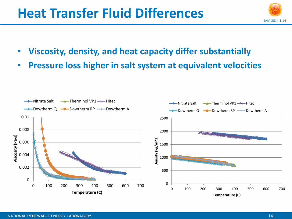
SAM 2014.1.14 Heat Transfer Fluid Differences

• Viscosity, density, and heat capacity differ substantially • Pressure loss higher in salt system at equivalent velocities

0

0.002

0.004

0.006

0.008

0.01

0 100 200 300 400 500 600 700

Visc

osity

(Pa-

s)

Temperature (C)

Nitrate Salt Therminol VP1 Hitec

Dowtherm Q Dowtherm RP Dowtherm A

0

500

1000

1500

2000

2500

0 100 200 300 400 500 600 700

Dens

ity (k

g/m

^3)

Temperature (C)

Nitrate Salt Therminol VP1 Hitec

Dowtherm Q Dowtherm RP Dowtherm A

15

SAM 2014.1.14 Solar field – Min/Max Flow Rate

• Field HTF Fluid = Hitec solar salt • Design loop outlet temp = 550°C

o Field inlet temperature related to boiling saturation temperature

• Min/Max single loop flow rate o Primary concern is maximum pressure drop o Therminol VP-1 velocity range [0.36, 4.97 m/s] o Method (1): Manually try different loop lengths and flow

rates in SAM o Method (2): Match pressure drops by iteratively solving

pipe pressure loss equations…

16

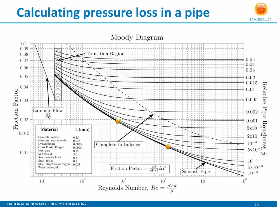
SAM 2014.1.14 Calculating pressure loss in a pipe

17

SAM 2014.1.14 (1) Establish a reference pressure loss

• Use Therminol-VP1 settings to calculate a reference pressure loss o Use maximum Therminol velocity

o Calculate Reynolds number

o Look up friction factor on Moody Chart

o Initial reference length is 𝑙𝑟𝑟𝑟 = 1.0

o Solve pressure loss eqn. for Δ𝑃𝑟𝑟𝑟

• We will try to set up the salt loop to match this ref. pressure constant

𝑉𝑇 = 5𝑚𝑠

𝑅𝑒𝑇 =𝜌𝑇𝑉𝑇𝐷𝜇𝑇

= 1.39e6

Δ𝑃𝑟𝑟𝑟 = 𝑓𝑟𝑇 𝑅𝑒𝑇𝜌𝑇 𝑉𝑇2𝑙𝑟𝑟𝑟

2𝐷 = 1610 𝑃𝑃

𝑓𝑟𝑇 = 0.011

𝐷 = 0.066 𝑚

18

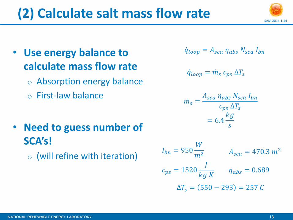
SAM 2014.1.14 (2) Calculate salt mass flow rate

• Use energy balance to calculate mass flow rate o Absorption energy balance o First-law balance

• Need to guess number of

SCA’s! o (will refine with iteration)

�̇�𝑙𝑙𝑙𝑙 = 𝐴𝑠𝑠𝑠 𝜂𝑠𝑎𝑠 𝑁𝑠𝑠𝑠 𝐼𝑎𝑏

�̇�𝑙𝑙𝑙𝑙 = �̇�𝑠 𝑐𝑙𝑠 Δ𝑇𝑠

�̇�𝑠 =𝐴𝑠𝑠𝑠 𝜂𝑠𝑎𝑠 𝑁𝑠𝑠𝑠 𝐼𝑎𝑏

𝑐𝑙𝑠 Δ𝑇𝑠

= 6.4𝑘𝑘𝑠

𝐴𝑠𝑠𝑠 = 470.3 𝑚2

𝜂𝑠𝑎𝑠 = 0.689 𝑐𝑙𝑠 = 1520𝐽

𝑘𝑘 𝐾

𝐼𝑎𝑏 = 950𝑊𝑚2

Δ𝑇𝑠 = 550 − 293 = 257 𝐶

19

SAM 2014.1.14 (3) Calculate velocity and new length

• Calculate velocity for mass flow rate

• Calculate Reynolds number

• Look up friction factor

• Solve pressure eqn. for length

• The new length is used to update the estimate of No. of SCA’s o Pressure highly nonlinear! Be conservative…

𝑉𝑠 =�̇�𝑠

𝜌𝑠𝜋𝐷2

2 = 1.02𝑚𝑠

𝑅𝑒𝑠 =𝜌𝑠 𝑉𝑠 𝐷𝜇𝑠

= 75254

𝑓 𝑅𝑒𝑠 = 0.0195

𝑙𝑟𝑟𝑟′ =Δ𝑃𝑟𝑟𝑟 2𝐷𝜌𝑠 𝑉𝑠2 𝑓𝑟𝑠

= 5.75

𝑁𝑠𝑠𝑠′ = 46?

𝑙𝑟𝑟𝑟′ = 2 → 𝑁𝑠𝑠𝑠′ = 16

20

SAM 2014.1.14 (4) Finally.. Iterate to convergence on L

Iter �̇�𝒔 kg/s

𝑽𝒔 m/s

𝑹𝒆𝒔 𝒇𝒇𝒔 𝑹𝒆𝒔 𝒍′ 𝑵𝒔𝒔𝒔

1 6.4 1.02 75254 0.0195 5.75 16

2 12.8 2.05 151247 0.0165 1.68 14

3 11.2 1.80 132802 0.017 2.11 16

• Number of SCA/HCE Assemblies = 14 • Max HTF Flow rate = 12.8 kg/s • Min HTF Flow rate = 1.75 kg/s

21

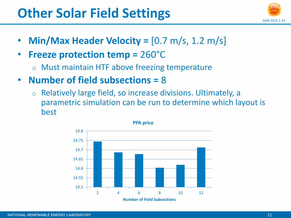
SAM 2014.1.14 Other Solar Field Settings

• Min/Max Header Velocity = [0.7 m/s, 1.2 m/s] • Freeze protection temp = 260°C

o Must maintain HTF above freezing temperature • Number of field subsections = 8

o Relatively large field, so increase divisions. Ultimately, a parametric simulation can be run to determine which layout is best

14.5

14.55

14.6

14.65

14.7

14.75

14.8

2 4 6 8 10 12Number of Field Subsections

PPA price

22

SAM 2014.1.14 Power Cycle – Dry Cooling

• Condenser type = Air-cooled • Ambient temp at design = 42°C

o Condensing temperature is 𝑇𝑠𝑎𝑎 + Δ𝑇𝐼𝑇𝐼 = 58𝐶 • Rated cycle conversion efficiency

o Prefer detailed external model, but… not always available o Reference cycle – Molten Salt power tower w/ 550°C steam

temperature at 41.2% gross efficiency o Assume 20°C salt-to-steam temperature drop o When in doubt, use Carnot scaling:

– 𝜂1 = 1 − 58+273.15𝟓𝟓𝟓+273.15

= 0.5977

– 𝜂2 = 1 − 58+273.15𝟓𝟓𝟓+273.15

= 0.5877

– 𝜂 = 0.412 𝜂2𝜂1

= 0.4051

23

SAM 2014.1.14 Power cycle – Other parameters

• Design gross output = 167 MWe o Increase design gross until the estimated nameplate

capacity meets the target

• Aux heater outlet set temp = 550°C o Not used in this example, but good practice

• Minimum required startup temp = 360°C o Trade HTF temperature for lower-efficiency cycle operation o Optimize!

24

SAM 2014.1.14 Thermal storage parameters

o Ensure HTF = Hitec Solar Salt – No intermediate HX is required

o Tank height = 15 – How reasonable is the calculated tank diameter?

o Parallel tank pairs = 2 o Cold tank heater set point = 260°C

– Match freeze protection temperature setting

o Hot tank heater set point = 525°C – Don’t allow significant decay in hot TES temperature

25

SAM 2014.1.14 Costs

• This example doesn’t consider detailed cost information! o Minor changes to reflect updated HTF

• Storage cost = 30 $/kWht • Power plant = 1200 $/kWe

26

Simulation & Results (in SAM)

27

SAM 2014.1.14 Optimizing thermal storage and solar multiple

28

SAM 2014.1.14 Optimizing…

29

SAM 2014.1.14 Comparison: MS vs Oil trough

MS Optimized Oil Trough Optimized Metric Value Metric Value Annual Energy 746,036,992 kWh Annual Energy 349,266,368 kWh PPA price 14.16 ¢/kWh PPA price 15.30 ¢/kWh LCOE Nominal 16.80 ¢/kWh LCOE Nominal 19.24 ¢/kWh LCOE Real 13.58 ¢/kWh LCOE Real 15.55 ¢/kWh Internal rate of return (%) 19.35% Internal rate of return (%) 19.50% Minimum DSCR 1.43 Minimum DSCR 1.44 Net present value ($) $137,266,240.00 Net present value ($) $73,059,680.00 Calculated ppa escalation (%) 1.00% Calculated ppa escalation (%) 1.00% Calculated debt fraction (%) 50.00% Calculated debt fraction (%) 50.00% Capacity factor 56.70% Capacity factor 39.90% Gross to Net Conv. Factor 0.93 Gross to Net Conv. Factor 0.93 Annual Water Usage 141,351 m3 Annual Water Usage 1,317,661 m3 Total Land Area 1961.13 acres Total Land Area 898.08 acres