modeling of rooftop packaged air conditioning equipment by
TRANSCRIPT

MODELING OF ROOFTOP PACKAGED
AIR CONDITIONING EQUIPMENT
by
MARK REICHLER
A thesis submitted in partial fulfillment of the requirements for the degree of
Master of Science (Mechanical Engineering)
at the
UNIVERSITY OF WISCONSIN-MADISON
1999

ii

i
Abstract
A large amount of the operating costs of a building is determined by the energy
requirements and the fuel consumptions of its heating, ventilation and air conditioning
system (HVAC-system). Simulation programs are used to determine the energy use in
buildings. These simulation programs are based on models for the type of HVAC equipment
used and models for determining the internal and external loads of the building. In this
project a model for rooftop packaged air conditioning units has been developed.
The model uses generally available manufacturer’s catalog data information to
determine the model parameters. Thus, the model is easy applicable. The system is modeled
by describing the performance of each component with mechanistic models. This method has
been successfully used to predict the performance of rooftop packaged air conditioning
systems and allows certain extrapolation of performance data.
The model has been developed with the Engineering Equation Solver (EES) software
package. A program has been written that allows determining the characteristic model
parameters based on manufacturer’s performance data and also allows creating extrapolated
performance data for different operating conditions. Originally developed with EES the
program can be also called directly by TRNSYS, a transient simulation program.

ii

iii
Acknowledgements
I consider myself fortunate to have done my graduate work at the Solar Energy
Laboratory of the University of Wisconsin. At this point special thanks go to the German
Academic Exchange Service (DAAD) that partially provided the funding for this project and
Professor Heisel from the University of Stuttgart, who managed the exchange program with
the University of Wisconsin. Also, I would like to thank the Professors of the Solar Energy
Laboratory for funding this project and giving me the opportunity to complete this research
project.
Special thanks go to my advisors Professor William Beckman and Professor John
Mitchell, who always kept me motivated during slow times of the project. They were always
very helpful and had many great ideas for this project. This work could not have been
accomplished without Prof. Sandy Klein and his Engineering Equation Solver (EES). Thus,
even for a student coming from the “SI-world”, as Professor John Mitchell used to say in his
lectures, the difficulties of doing calculations in the English unit system were overcome.
Meanwhile, for myself 1 ton rather represents 12,000 Btu/hr of refrigeration capacity, which
is approximately 3.5 kW, than representing the mass of 2000 pounds.
I am really thankful to the professors of the Solar Energy Laboratory for letting me
further pursue my education at the Solar Lab. Not only did I further improve my engineering
skills, but when preparing for the seminars I also significantly enhanced my baking skills.
Also, I have greatly enjoyed the friendly environment in the Solar Lab, having met many

iv
students from the country and around the world, too many to mention them all. I will
definitely take many good memories of that time with me.
In times of hard working, one need a place to relax. Fortunately, I had this place! I
want to thank my roommates and friends for having a great time in Madison and lots of fun.
Especially, I want to thank Sarah for “beta-reading” my thesis and giving me helpful advice
concerning my writing style.
Last but not at least, I want to thank my parents who always supported me in my
education and by having done this they pay a great contribution to my stay abroad here at the
University of Wisconsin and this work.

v
Table of Contents
ABSTRACT i
ACKNOWLEDGEMENTS iii
TABLE OF CONTENTS v
LIST OF FIGURES ix
LIST OF TABLES xi
NOMENCLATURE xiii
CHAPTER 1
INTRODUCTION 1
1.1 The Need for Air Conditioning 1
1.2 Project Outline 1
CHAPTER 2
SYSTEM DESCRIPTION 5
2.1 Air Conditioning Systems 5
2.2 Rooftop Packaged Units 6
2.3 Available manufacturer data 8

vi
CHAPTER 3
COMPRESSOR MODELING 11
3.1 Compressors 11
3.1.1. Reciprocating Compressors 11
3.1.2. Scroll Compressors 14
3.2 Compressor Modeling 16
3.2.1. Mass Flow Rate 17
3.2.2. Compressor Power 19
3.2.3. Parameter Identification 20
3.3 Validation of the Compressor Model 21
3.3.1. Objective Function for Parameter Fitting Procedure 22
3.3.2. Model Validation for Reciprocating Compressors 23
3.3.3. Model Validation for Scroll Compressors 32
3.4 Conclusions 39
CHAPTER 4
HEAT EXCHANGER MODELING 41
4.1 Introduction 41
4.2 Heat Exchangers for Refrigeration Applications 43
4.3 Heat Exchanger Modeling 46
4.3.1. Effectiveness-NTU Method for Dry Cooling Coils and Condensers 46
4.3.2. Effectiveness-NTU Method for Wet Cooling Coils 48
4.4 Conductance Area Product for Direct Expansion Coil 56
4.5 Conductance Area Product for Condenser Coil 59

vii
4.6 Heat Exchanger Model Validation 62
4.6.1. Objective Function for Parameter Fitting Procedure 63
4.6.2. Validation of the Evaporator Model 63
4.6.3. Validation of the Condenser Model 68
4.7 Conclusions 71
CHAPTER 5
SYSTEM MODELING 73
5.1 Introduction 73
5.2 The Vapor Compression Cycle 74
5.3 System Modeling 76
5.4 Model Validation 80
5.4.1. Validation for Idealized Vapor Compression Cycle 84
5.4.2. Effect of Number of Data Points 97
5.4.3. Effect of Superheat 99
5.4.4. Effect of Subcooling 102
5.4.5. Fans 105
5.4.6. Heating 106
5.4.7. Part load modeling 106
5.4.8. Conclusions 107
CHAPTER 6
CONCLUSIONS AND RECOMMENDATIONS 109
6.1 Conclusions 109
6.2 Future Work 112

viii
APPENDIX 115
Appendix A: Model Results for Rooftop Packaged Unit 50 EJ 034 115
Appendix B: Model Results for Rooftop Packaged Unit 48 TJ 016 and 48 TJ 024 128
Appendix C: EES-code for compressor model (mass flow rate) 135
Appendix D: EES-code for compressor model (power) 139
Appendix E: EES-code for vapor compression cycle 143
Appendix F: EES-code for direct expansion coil model 148
Appendix G: EES-code for 3-parameter condensing coil model 154
Appendix H: EES-code for roofop packaged model 156
Appendix I: EES-code for 6-parameter condensing coil model 166
Appendix J: Use of the EES-program RTPU 170
BIBLIOGRAPHY 175

ix
List of Figures
Figure 2.1: Survey of cooling equipment used in commercial buildings 1995 ........................ 5
Figure 2.2: Components of a rooftop packaged unit and schematic air flow [Trane, 1981] .... 8
Figure 3.1: Classification of reciprocating compressors [Wang, 1993] ................................. 12
Figure 3.2: Schematic indicator diagram for a reciprocating compressor .............................. 13
Figure 3.3: Scroll compressor with scroll compression process [Wang, 1993]...................... 15
Figure 3.4: Predicted mass flow rate for data sets a to d ........................................................ 27
Figure 3.5: Predicted power draw for data sets a to d............................................................. 28
Figure 3.6: Predicted mass flow rate with extrapolated data points using data set d ............. 29
Figure 3.7: Predicted compressor power draw with extrapolated data points ........................ 30
Figure 3.8: Compressor mass flow rate map with catalog and predicted mass flow rate ....... 31
Figure 3.9: Compressor power draw map with catalog and predicted compressor power draw
.......................................................................................................................................... 31
Figure 3.10: Predicted mass flow rate for scroll compressor (8)............................................ 33
Figure 3.11: Predicted compressor power draw for compressor (8)....................................... 34
Figure 3.12: Power versus pressure ratio for compressor (8) ................................................. 35
Figure 3.13: Mass flow rate versus pressure ratio for compressor (8).................................... 36
Figure 3.14: Predicted power draw with modified scroll compressor model......................... 38
Figure 3.15: Predicted compressor power draw with extrapolated data points for data set b 38
Figure 4.1: Schematic drawing of a dry type direct expansion coil........................................ 44
Figure 4.2: Schematic of a counterflow cooling coil .............................................................. 50
Figure 4.3: Generalized thermal circuit for a coil ................................................................... 54
Figure 4.4: Different heat transfer regions in a condenser...................................................... 60
Figure 4.5: Effect of parameter C2 on the error in the fitting procedure................................. 66
Figure 4.6: Extrapolation of data set a to lower and higher suction temperatures.................. 67
Figure 4.7: Extrapolation of data set b to lower and higher air entering temperatures........... 67
Figure 4.8: Extrapolation of data set c to higher and lower face velocities ............................ 68
Figure 4.9: Performance prediction with the condenser model .............................................. 70
Figure 5.1: Single stage vapor compression cycle .................................................................. 74

x
Figure 5.2: Vapor compression cycle in pressure-enthalpy diagram...................................... 76
Figure 5.3: Schematic pressure-enthalpy diagram.................................................................. 79
Figure 5.4: Effect of parameter C2 on error in optimization................................................... 85
Figure 5.5: Predicted versus catalog total evaporator heat transfer rate for data set ( a ) ....... 86
Figure 5.6: Predicted versus catalog sensible evaporator heat transfer rate for data set ( a ) . 86
Figure 5.7: Predicted versus catalog total evaporator heat transfer rate for data set ( d )....... 87
Figure 5.8: Predicted versus catalog sensible evaporator heat transfer rate for data set ( d ) . 87
Figure 5.9: Predicted versus catalog condenser heat transfer rate for data set ( a ) ................ 89
Figure 5.10: Predicted versus catalog condenser heat transfer rate for data set ( d ).............. 89
Figure 5.11: Predicted versus catalog condenser heat transfer rate for data set ( a ) using
detailed model .................................................................................................................. 91
Figure 5.12: Predicted versus catalog condenser heat transfer rate for data set ( d ) using
detailed model .................................................................................................................. 91
Figure 5.13: Input variables, output variables, and parameters used in rooftop packaged air
conditioning model........................................................................................................... 92
Figure 5.14: Predicted compressor power draw for model parameters calculated with data set
( a ) ................................................................................................................................... 94
Figure 5.15: Predicted total capacity for model parameters calculated with data set ( a ) ..... 94
Figure 5.16: Predicted sensible capacity for model parameters calculated with data set ( a ) 95
Figure 5.17: Predicted compressor power draw for model parameters calculated with data set
( d ) ................................................................................................................................... 96
Figure 5.18: Predicted total capacity for model parameters calculated with data set ( d ) ..... 96
Figure 5.19: Predicted sensible capacity for model parameters calculated with data set ( d ) 97
Figure 5.20: Effect of superheat on power prediction .......................................................... 100
Figure 5.21: Effect of superheat on total capacity prediction............................................... 100
Figure 5.22: Effect of superheat on sensible capacity prediction......................................... 101
Figure 5.23: Effect of subcooling on power prediction........................................................ 103
Figure 5.24: Effect of subcooling on total capacity prediction............................................. 103
Figure 5.25: Effect of subcooling on sensible capacity prediction....................................... 104

xi
List of Tables
Table 2.1: Available catalog information on rooftop packaged units from different
manufacturers..................................................................................................................... 9
Table 3.1: Comparison of reciprocating and scroll compressors [Wang, 1993] .................... 16
Table 3.2: Compressor data for five different reciprocating compressors.............................. 23
Table 3.3: Compressor parameters for compressors (1) to (5)............................................... 25
Table 3.4: Data sets a to d used for determining compressor parameters for compressor (5) 26
Table 3.5: Compressor parameters for data sets a to d ........................................................... 26
Table 3.6: Scroll compressor data........................................................................................... 32
Table 3.7: Scroll compressor parameters ................................................................................ 33
Table 3.8: Resulted errors in power draw prediction for compressors (6) to (8).................... 37
Table 3.9: Effect of number of fitting points on curve fit parameters and power draw
prediction.......................................................................................................................... 37
Table 4.1: Effectiveness-NTU relations for sensible heat exchangers and wet cooling coils 52
Table 4.2: Direct expansion coil used for model validation................................................... 64
Table 4.3: Heat exchanger parameters for direct expansion coil for data sets a to c .............. 65
Table 4.4: Condensing coil used for model validation ........................................................... 69
Table 4.5: Heat exchanger parameters for condensing coil .................................................... 69
Table 4.6: Errors for performance prediction for the condensing coil.................................... 70
Table 5.1: Rooftop packaged units ......................................................................................... 80
Table 5.2: Compressor parameters for packaged unit ( 3 ) ..................................................... 82
Table 5.3: Data sets ( a ) to ( d ) for determining the model parameters ................................ 83
Table 5.4: Evaporator model parameters for rooftop packaged unit ( 3 ) for data sets ( a )
to ( d ) ............................................................................................................................... 84
Table 5.5: Condenser model parameters for rooftop packaged unit ( 3 ) for data sets ( a )
to ( d ) ............................................................................................................................... 88
Table 5.6: Parameters for detailed condenser model for rooftop packaged unit ( 3 ) for data
sets ( a ) to ( d )................................................................................................................. 90
Table 5.7: Performance prediction of the rooftop packaged air conditioning model ............. 93

xii
Table 5.8: Effect of number of data points on performance prediction.................................. 98

xiii
Nomenclature
a parameter for compressor efficiency
A area
Ao outer heat transfer area
b parameter for compressor efficiency
C clearance factor
C0 coefficient in heat transfer correlation
c1..3 coefficients in polynomial expression E
C1..9 heat exchanger parameter
fictitiouspc , fictious specific heat
Cf coefficient in heat transfer correlation
Cmax maximum capacitance rate
Cmin minimum capacitance rate
cp specific heat at constant pressure
Cr capacitance rate ratio
cs saturation specific heat
cv specific heat at constant volume
D tube diameter
Dh hydraulic diameter
∆hr enthalpy difference in condensing region

xiv
∆p pressure drop parameter
E polynomial expression
ε heat exchanger effectiveness
F coefficient in heat transfer correlation for condensation
η0 fin efficiency
ηcomb combined efficiency
ηv volumetric efficiency
g gravitational constant
h1..4 enthalpies for state points
ha enthalpy of air
hc convection coefficient
hfg enthalpy of vaporization
hsat enthalpy of saturated air
hA overall conductance area product
hAi inner conductance area product
hAo outer conductance area product
k thermal conductivity
m exponent in heat transfer correlation
m& mass flow rate
m* capacitance rate ratio for wet coil analysis
µ dynamic viscosity

xv
n polytropic exponent
N number of data points
NTU number of transfer units
NTU* number of transfer units used in the wet coil analysis
NTUi number of transfer units for inner heat transfer
NTUo number of transfer units for outer heat transfer
ν kinematic viscosity
NuD Nusselt number
mOF & objective function for mass flow rate
POF objective function for power
QOF & object function for heat transfer rate
ω humidity ratio of air
P power
p pressure
Pr Prandtl number
Q& heat transfer rate
Rtube thermal resistance of the tube
Rcom compression ratio
ReD Reynolds number
ρ density
RPM motor speed

xvi
T temperature
u velocity
U*A overall heat transfer area coefficient product based on enthalpies
UA overall heat transfer area coefficient product
UAi inner overall heat transfer area coefficient product
v specific volume
va..d specific volume at state point a to d
Va..d volume at state point a to d
Vdisp displacement volume
ustd face velocity
W work
x refrigerant quality
z parameter in expression for compressor power draw of scroll
compression process
Additional Subscripts
a air
act actual
c cold
calc calculated
cat catalog

xvii
comp compressor
cond condenser
db dry bulb
dis discharge
dp dew point
evap evaporator
f liquid
g vapor
h hot
i at inlet state
max maximum
mean mean
min minimum
o at outlet state
r refrigerant, at refrigerant temperature
s at surface temperature
sat saturated
sens sensible
suc suction
th theoretical
tot total
w water

xviii
wb wet bulb

1
Chapter 1 Introduction
1.1 The Need for Air Conditioning
Although some people might regard air conditioning as a luxury, in certain areas
having air conditioning is a must. One does not feel comfortable if the temperature and
humidity level is too high. Air conditioning affects not only personal comfort, but also
economics. If people feel comfortable, their productivity is generally better than if they work
under uncomfortable conditions. Thus, air conditioning is and will be more and more needed
in our world.
1.2 Project Outline
When designing an air conditioning system for a new building or replacing an air
conditioning system in an old building, it is necessary to know which air conditioning system
or which products would operate best and be most cost effective. One convenient way to
figure out the best solution for the system design is to run computer simulations, in which the
whole building with its equipment is modeled. Therefore, models have to be available that
predict the performance of air conditioning equipment under different operating conditions.
The goal of this project is to develop a model of a rooftop packaged air conditioning
system suitable for use in simulations. The model uses available manufacturer’s catalog data
only. The model should fit the catalog data accurately and allow a satisfactory extrapolation
over a wide range of operating conditions.

2
To develop the model, the different components of the system such as compressor,
evaporator, condenser and expansion valve have to be modeled. Different approaches exist to
model the behavior of those components.
One method for modeling the performance of a component is to use a curve fit
approach using a polynomial representation. It is easy to represent the characteristics of a
component, given that there are enough catalog points to get a good curve fit. The resulting
equations, however, have no physical meaning, and a prediction of the component
performance outside the range of the fitted data may be very inaccurate.
Another modeling technique is to describe the behavior of a component using
mechanistic models. This requires a detailed knowledge of characteristic parameters such as
geometric specifications, fin efficiencies, or other quantities. Such detailed information is
generally not found in manufacturer’s catalogs.
To avoid the problems of uncertain extrapolation with a polynomial representation
and to accommodate the lack of specific information about the system’s components for a
complex model, a semi-mechanistic modeling technique is used in this project. The
characteristic performance parameters for each component will be first defined. Those
performance parameters contain all specific characteristics of the system’s components.
Parameter values are then obtained by fitting the model to the catalog data. The resulting
model should allow reasonable extrapolation over a wide operating range.
Listed below are the steps that were followed to achieve the project goal:
• Performance data of rooftop packaged air conditioning units from different manufacturers
were collected. Available manufacturer’s data were checked for use in the model. The

3
manufacturer’s data should be given over a wide range of operating condition to allow
performance prediction of the model and for the extrapolation ability of the model to be
checked.
• The literature was searched for modeling techniques for the whole system as well as for
the single components used in a rooftop packaged unit.
• Performance data were collected for the individual components (compressor, evaporators,
and condensers) used in rooftop packaged units. The developed models for these
components were evaluated by using these data. Thus, models could be used in the
rooftop packaged air conditioning unit model.
• A general model for rooftop packaged units based on manufacturer’s catalog data to
predict performance was developed. Each of the system components is modeled.
• The model of the rooftop packaged air conditioning unit was evaluated over the whole
operating range and extrapolation ability of the model was tested.
• The number of data points used to predict system’s performance accurately was
determined.
A software package was developed with the Engineering Equation Solver that allows
easy computation of extrapolated catalog data for rooftop packaged air conditioning units
with different capacities. Also, it allows this model to be called by TRNSYS, which is a
transient simulation program to perform energy calculations.

4

5
Chapter 2 System description
2.1 Air Conditioning Systems
Air conditioning systems can be divided into packaged air conditioning systems and
central air conditioning systems. Usually, central air conditioning systems are used for entire
buildings where the total cooling load is very high. Packaged units are often used if cooling
demand is lower and cooling is needed for just a few rooms.
In 1995, a survey was made by the Energy Information Administration of the
Department of Energy of the United States, in which the end-use equipment for space
cooling was recorded for commercial buildings. Figure 2.1 shows the end-use equipment for
space cooling as a percentage of the total cooled floor area in commercial buildings.
Figure 2.1: Survey of cooling equipment used in commercial buildings 1995
23.9
10
8.9
7.8
12.1
37.3
0 5 10 15 20 25 30 35 40
Packaged AC Units
Central Chillers
Residential-Type Central AC
Heat Punps
Individual Air Conditioners
Others
Percent of Cooled Floor Space

6
According to Figure 2.1, unitary packaged systems are by far the most commonly
used air conditioning equipment in commercial buildings in the United States. 1,242,000
buildings out of 3,381,000 buildings were cooled by packaged air conditioning units. This
corresponds to 37.3 % of the total cooled floor area of 3344 million square meters (36,001
million square feet) in commercial buildings. 23.9 % of the total floor area was cooled by
central chillers. Only 96,000 commercial buildings had a central chiller as cooling
equipment, which reflects that central chillers are mainly used if higher cooling capacity is
required.
2.2 Rooftop Packaged Units
A packaged air conditioning unit is a self-contained air conditioner. It provides the
cooling, heating and the motion of the air. Packaged units can be classified into three general
types of units, the indoor packaged units, the split packaged units and the rooftop packaged
units. The indoor and split packaged units differ from rooftop packaged units in arrangement
and kind of equipment used. They consist of two main modules, an indoor air handling unit
and an outdoor condensing unit. The condensing units are often water-cooled. This project
is concentrated on rooftop packaged air conditioning units only. Thus, a generalized model
can be developed for this type of unit, since the components used in rooftop packed units,
such as compressor or condenser types, are mostly the same types.
Rooftop packaged units come as one single package that is ready to be mounted on a
rooftop. All the components needed for cooling, heating, and air movement are assembled in

7
a steel casing. Rooftop packaged units can be classified according to the type of heating they
supply. There are rooftop packed units with either electric heating or gas-fired heating. The
heating can also be provided by a heat pump. However, electric heat and gas-fired furnaces
are mainly used. The available cooling capacity of common packaged rooftop units ranges
from 10 kW (3 tons) to 850 kW (241 tons). The air flow rate covers a range from 400 l/s
(850 ft3/min) to 37,800 l/s (80,000 ft3/min).
Rooftop packaged units are equipped either with a supply fan only or, if needed,
an additional return air fan. As the air is delivered by the return fan, the air is mixed with
outdoor air. Then the mixed air is drawn through filters, which are usually low or medium
efficiency air filters. By passing through the cooling coils, the air stream is cooled down to
some set point temperature. Often dehumidification occurs. Then, the air enters the heating
section, where it is heated up to the set point temperature, if needed. As mentioned before,
the heating is done by either electric heating, gas fired heating or a heat pump. After drawn
through the heating section the supply air stream leaves the packaged unit and enters the
ductwork of the building.
The cooling capacity is provided by a vapor compression cycle, with reciprocating or
scroll compressors as the central component. The cooling coils are always direct expansion
coils in rooftop packaged units. Units with a higher cooling capacity often have two separate
refrigerant circuits in the evaporator for better capacity control. The condenser is designed of
fin air-cooled condensing coils in which the refrigerant vapor is liquefied.
Figure 2.2 illustrates the arrangement of the main components of a rooftop packaged
unit described above. Also, the air flow through the unit is shown schematically.

8
Figure 2.2: Components of a rooftop packaged unit and schematic air flow [Trane, 1981]
2.3 Available manufacturer data
Almost all large manufacturers of rooftop packaged air conditioning units have
catalogs available for their products. To build a model that is generally applicable, catalog
information from different manufacturers (Trane, Carrier, AAON) was collected and
available inputs were determined.
In all catalogs the total cooling capacity as well as the sensible capacity is given as a
function of volume flow rate, ambient temperature and return air conditions. Carrier also
provides the compressor power draw for these operating points, which is a necessary
input for the model. In addition, the compressor type and its performance in form of a few
operating points or a compressor map has to be known. Knowing this information, the model
developed in this project can be applied to any rooftop packaged unit. Table 2.1 presents the
Condenser
Supply fan Condenser fan Outdoor air
Return air Supply air Cooling coil
Heating section
Compressor
Filters
Return fan

9
data that is used as input for the rooftop packaged air conditioning model. Also, it shows the
availability of those data for three different manufacturers.
Table 2.1: Available catalog information on rooftop packaged units from different manufacturers
Manufacturer
Available Catalog Data Trane Carrier AAON
UNIT
Entering Wet Bulb (evaporator) X X X
Entering Dry Bulb (evaporator) X X X
Ambient Temperature X X X
Total Cooling Capacity X X X
Sensible Cooling Capacity X X X
Compressor Power Input X
COMPRESSOR
Compressor Type X X
Quantity X X X
CONDENSER FAN
Volume Flow Rate X X X
Power Input X X X
EVAPORATOR COIL
Face Area X X X
EVAPORATOR FAN
Volume Flow Rate (evaporator) X X X
Power Input X X X

10

11
Chapter 3 Compressor Modeling
3.1 Compressors
The refrigeration compressor is the central component of a vapor compression cycle.
It raises the pressure and provides the circulation of the refrigerant. In rooftop packaged units
either reciprocating compressors or scroll compressors are used. Thus, a model for these both
compressor types is necessary. A compressor model will be developed for reciprocating
compressors and will then be applied to scroll compressors.
3.1.1. Reciprocating Compressors
Reciprocating compressors are positive displacement compressors. They are used for
applications such as rooftop packaged units with a cooling capacity of up to about 210 kW
(60 tons). Reciprocating compressors are classified as hermetic, semi-hermetic and open
compressors. The number of cylinders ranges from one up to eight or more cylinders. Often
more than one compressor is coupled together to achieve higher cooling capacities for large
systems. If more than one compressor is used in rooftop packaged units, part load operation
can be achieved by turning off one or more compressors. Often, compressors with more than
one cylinder are also equipped with an unloading mechanism, which permits the unloading of
one or more cylinders to achieve better part load performance. The unloading is done by
leaving the suction valve of the unloaded cylinders open.

12
Figure 3.1 shows the three types of reciprocating compressors, (a) hermetic
compressors, (b) semi-hermetic compressors, and (c) open compressors.
Figure 3.1: Classification of reciprocating compressors [Wang, 1993]
( a )
( b )
( c )

13
Most packaged units use semi hermetic compressors, which means that the motor and
compressor unit are mounted in one housing. The main difference between a hermetic and a
semi-hermetic compressor is that the semi-hermetic compressor can be taken apart to do
maintenance work.
Figure 3.2: Schematic indicator diagram for a reciprocating compressor
Figure 3.2 illustrates the compressor cycle occurring in a reciprocating compressor.
At point d the suction valve opens and vaporized refrigerant leaving the evaporator enters the
cylinder. While the piston moves down to its bottom dead center (point a), the cylinder
volume is filled with vapor. Reaching the bottom dead center the suction valve closes and the
compression process starts. At point b the pressure reaches a sufficient level to open the
Vdisplacement Vclearance
Pcondenser
Pevaporator
c b
ad
Discharge Valve
Suction Valve

14
exhaust valve and refrigerant is discharged to the condenser. This process takes place till the
piston reaches its top dead center (point c). The volume that is now left is called the clearance
volume. The gas expands as the piston moves to point d. The volume from the bottom to the
top dead center is called the displacement volume. These both variables, clearance volume
and displacement volume, are important parameters in the compressor model used for
modeling the system. The pressures shown in the schematic indicator diagram above are not
the real condensing and evaporating pressures, since pressure drops occur through the suction
and exhaust valves. These pressure drops, however, are relatively small compared to the
dimension of the total pressure.
3.1.2. Scroll Compressors
Similar to reciprocating compressors, scroll compressors are also positive
displacement compressors. They are used in rooftop packaged units with a cooling capacity
in the range from 35 kW (10 tons) to 420 kW (120 tons), especially in those systems with a
large cooling capacity. This is due to the fact that scroll compressors operate more efficiently
than reciprocating compressors do. Also, they are more reliable, operate more quietly and
smoothly, which makes them also increasingly popular for smaller units. In Figure 3.3 a
scroll compressor is shown with its compression process.

15
Figure 3.3: Scroll compressor with scroll compression process [Wang, 1993]
The scroll compression process takes place between two scrolls. One scroll is
stationary and fixed. The other scroll is assembled with a phase difference of 180° and moves
in an orbit around the center of the other scroll. The suction process takes place at the lateral
openings. Vapor refrigerant enters the space between the two scrolls. When the orbiting
scroll moves, the space between the two scrolls becomes sealed off and the compression
process takes place. The space between the scrolls decreases continuously and by reaching

16
the center of the stationary scroll, the compressed hot refrigerant is discharged through a
small opening in the center. Intake, compression, and discharge occur simultaneously in
scroll compressors. Table 3.1 shows the characteristics of reciprocating and scroll
compressors by comparison.
Table 3.1: Comparison of reciprocating and scroll compressors [Wang, 1993]
Reciprocating compressors Scroll compressors
Compression process characteristic positive displacement positive displacement
Refrigeration capacity < 700 kW (200 tons) up to 200 kW (60 tons)
Refrigerants HCFC-22, HFC-134a HCFC-22
Volumetric efficiency 0.92 to 0.68 (at Rcom = 1 to 7) > 0.95 (at Rcom = 4)
Compressor efficiency 0.83 to 0.75 (at Rcom = 4 to 7) 5 to 10 % higher
Capacity control on-off, cylinder unloader on-off, scroll unloader
Reliability reliable more reliable
Application to rooftop packaged
units up to 200 kW (60 tons)
35 kW (10 tons) up to
420 kW (120 tons)
3.2 Compressor Modeling
Many approaches for modeling refrigeration compressors have been developed.
Modeling techniques for reciprocating and scroll compressors are of special interest for this
project, since these are the types of compressors used in rooftop packaged units. Simple
compressor models, which are found in thermodynamic textbooks such as Moran and

17
Shapiro (1992), often assume the compressor to be adiabatic. Inefficiencies are taken into
account by defining an isentropic compressor efficiency. More detailed compressor models
such as presented by Shapiro (1995) also take heat transfer into account by developing
expressions for the heat loss of the compressor.
Another possibility to describe the performance of compressors is to use polynomial
expressions for the mass flow rate and the compressor power draw. Stoecker (1971) proposed
polynomial expressions for the compressor power draw and the capacity. Each of these
expressions contains nine coefficients that have to be determined. Thus, an accurate
performance prediction is possible if one has enough data points to determine these
coefficients. However, extrapolation outside of the range of the data that were used for
determining model parameters is uncertain with this method.
For this project a semi-empirical compressor model presented by Jähnig (1999) is
used. This model allows certain extrapolation outside of the range of the fitted data, and is
described in the following section.
3.2.1. Mass Flow Rate
For predicting the mass flow rate of reciprocating compressors, a model, known as
the volumetric efficiency model presented by McQuiston and Parker (1988), is used. The
volumetric efficiency is defined as the ratio of the actual mass flow rate of the refrigerant to
the theoretical possible mass flow rate of the compressor. Theoretical possible mass flow rate

18
means that the displacement volume is fully filled with refrigerant vapor at the suction inlet
state. Thus, using the notation of Figure 3.2, the theoretical mass flow rate can be written as:
( )RPM
v
VVm
suc
cathr ⋅
−=,
& ( 3-1 )
The actual mass flow rate is given by equation ( 3-2 ):
( )RPM
v
VVm
a
daactr ⋅
−=,
& ( 3-2 )
Consequently, the volumetric efficiency can be written as:
( )( ) ada
succa
actr
thr
v vVV
vVV
m
m
⋅−⋅−
==,
,
&
&η ( 3-3 )
The compression and the expansion can be described by equations ( 3-4 ) and ( 3-5 )
as polytropic processes between two states:
nbdis
nasuc VpVp ⋅=⋅ ( 3-4 )
nddis
ncsuc VpVp ⋅=⋅ ( 3-5 )
The polytropic exponent n determines the process occurring between two states. For
n=0 the process is an isobaric, for n=1 the process is isothermal. For the compressor model
the compression process is assumed to be reversible and adiabatic. Thus, the exponent n can
be calculated as the ratio of specific heat at constant pressure and the specific heat at constant
volume.
rv
rp
c
cn
,
,= ( 3-6 )

19
Knowing the displacement volume of the compressor
cadisp VVV −= ( 3-7 )
and defining the clearance factor of the compressor as
ca
c
VV
VC
−= ( 3-8 )
the definition of the volumetric efficiency can be written in terms of the clearance
factor, the polytropic exponent, and the pressure ratio as well as the specific volume at inlet
and discharge conditions:
RPM
RPM
v
v
p
pCC
m
m
a
sucn
suc
dis
thr
actr
V ⋅⋅
⋅−+==
1
,
,1
&
&η ( 3-9 )
3.2.2. Compressor Power
The work per mass of refrigerant vapor required during compression process can be
calculated by the following equation:
∫∫ −=c
d
b
a
th vdpvdpW ( 3-10 )
Performing the integration for a polytropic process, the work per compressor cycle
per mass for polytropic processes is given by:
−
⋅⋅⋅
−=
−
11
1n
n
suc
dissucsucth
p
pvp
n
nW ( 3-11 )

20
Then the compressor power can be calculated by:
−
⋅⋅⋅
−⋅=
−
11
1
,
nn
suc
dissucsucactrth
p
pvp
n
nmP & ( 3-12 )
3.2.3. Parameter Identification
The expressions above for the volumetric efficiency and the work per compressor
cycle can be used to determine the mass flow rate as well as the compressor power draw.
However, they do not take inefficiencies into account such as friction losses, heat loss, or
pressure drops. Consequently, using these equations for modeling the compressor
performance is not applicable to a system. By introducing parameters that account for
inefficiencies, the model can describe the compressor performance accurately. Thus, the
compressor model can be used for system modeling. Jähnig (1999) proposed to introduce a
pressure drop parameter and parameters for the compressor efficiency. The following
parameters are used to model the compressor performance. The values were determined by
fitting the model to catalog data.
C - clearance factor
∆p - pressure drop parameter for suction pressure
a - parameter for compressor efficiency
b - parameter for compressor efficiency

21
The expression for the mass flow rate is written in terms of the clearance factor. The
clearance factor is a function of the geometry only and is therefore a fixed number for each
compressor. The clearance volume, however, is usually not provided by the manufacturer
and was determined by fitting compressor performance data to the compressor model.
The pressure drop parameter accounts for pressure drops across the valves. Pressure
drops can be found on the suction line as well as on the discharge line. The following
expression was found to work best. Although it accounts only for the pressure drop on the
suction line, it provides a good fit to the catalog data.
( )ppp evapsuc ∆−⋅= 1 ( 3-13 )
Jähnig (1999) defined a combined efficiency as the ratio of the theoretical required
compressor power draw to the actual power draw. It accounts for inefficiencies such as motor
inefficiencies, mechanical inefficiencies, and heat transfer in the compressor. The combined
efficiency is defined by the following equation:
sucact
thcomb
p
ba
P
P +==η ( 3-14 )
where a and b need to be determined by fitting to catalog data.
3.3 Validation of the Compressor Model
Compressor data were collected from different manufacturers. The compressor model
was validated by using the given manufacturer’s catalog data. Having developed the model

22
originally for reciprocating compressors, the capability of predicting the performance of
scroll compressors was also tested.
3.3.1. Objective Function for Parameter Fitting Procedure
The parameter values are obtained by fitting the compressor model to manufacturer’s
catalog data. The objective function is a mean weighted RMS error, which measures the
mean percent deviation of the calculated data points from the mean value of all catalog data
points used for fitting.
Thus, the objective functions for determining the parameters used to predict the mass
flow rate and the power are given by equation ( 3-15 ) and ( 3-16 ).
For mass flow rate:
N
m
mm
OF
N
imeanr
calcrcatr
m
∑=
−
=1
2
,
.
,
.
,
.
.
( 3-15 )
For compressor power:
N
P
PP
OF
N
i mean
calccat
P
∑=
−
= 1
2
( 3-16 )
First the parameters for the mass flow rate were determined in the fitting process.
Having determined these parameters, they were used in the fitting process to determine the
parameters used in the model for the power prediction. The four parameters could be fitted at
23
the same time. Parameter values for the mass flow rate, however, also affect the power
prediction. Parameter values for the mass flow rate could be found, which would yield to a
better power fit, while the mass flow rate fit would be worse if all parameters were fitted at
the same time.
3.3.2. Model Validation for Reciprocating Compressors
The collected compressor data for reciprocating compressors covers a capacity range
from 3.5 kW (1 ton) up to 53 kW (15 tons). Table 3.2 lists some of the compressors modeled
in this project to validate the compressor model.
Table 3.2: Compressor data for five different reciprocating compressors
Compressor (1) (2) (3) (4) (5)
Manufacturer Trane Trane Trane Carlyle Carlyle
Model No. 16 BH 143
YZ 1
16 GH 673
LM 1 G 14 CRHC 100 06 DE 8241 06 DE 5371
Type hermetic hermetic hermetic semi-hermetic semi-hermetic
Capacity
kW (tons) 4 (1) 18 (5) 35 (10) 33 (9) 52 (15)
Displacement
[ft3/min] 3.148 12.534 25.5 23.9 37.1
Motor speed
[min-1] 3500 3500 3450 1750 1750
Cylinder 1 2 3 6 6

24
For determining the compressor parameters C, ∆p, a, and b compressor data were
used in which the compressor power draw and capacity were given as a function of the
evaporating temperature and the condensing temperature. Available compressor data refer to
rating conditions according to ARI Standard 520. Thus, compressor performance data refer to
–9.4 °C (15 °F) subcooling and –6.7 °C (20 °F) superheat. Data of compressors (4) and (5)
refer to –9.4 °C subcooling and superheat.
Table 3.3 lists the calculated model parameters for compressors (1) to (5). Fourteen
data points covering the catalog range of evaporating and condensing temperature were
chosen for calculating the model parameters. For these compressors, the clearance factor,
which is used as a curve fit parameter, is in the range of 0.071 to 0.121. Realistic values,
which are difficult to obtain from manufacturers, are probably around 0.05. Manufacturers
try to minimize the clearance volume as far as possible. This is due to the fact that the
volumetric efficiency increases with decreasing clearance volume, which means
consequently an enhanced compressor performance.

25
Table 3.3: Compressor parameters for compressors (1) to (5)
Compressor (1) (2) (3) (4) (5)
Number of
data points 16 16 14 14 14
C 0.121 0.084 0.097 0.076 0.071
∆p 0.075 0.050 0.068 0.091 0.094
a 0.735 0.727 0.682 0.743 0.716
b -0.482 -0.257 -0.104 -0.261 -0.191
OFm [%] 6.4 2.0 0.9 1.4 2.0
OFP [%] 10.6 3.1 4.3 2.0 2.9
3.3.2.1 Required Number of Data Points for Fitting
From Table 3.2, compressor (5) was chosen to analyze the effect of the number of
data points used in the fitting process on the compressor performance. Table 3.4 contains the
data sets (a, b, c and d) used for determining the compressor parameter for four different
numbers of given operating points. Compressor parameters were determined using five, eight
and fourteen data points. Table 3.5 lists the calculated compressor parameters for data sets a
to d. As a general rule data points should be selected as a combination of low and high values
for each cataloged operating variable. In the case of the compressor, the operating variables
are the condensing and evaporating temperatures. Thus, at least four data points should be
selected for the fitting process to get a good curve fit. By using additional data points in the
fitting process, model prediction can be improved.

26
Table 3.4: Data sets a to d used for determining compressor parameters for compressor (5)
Data
point
Tevaporator
[°C]
Tcondenser
[°C]
Mass flow
[kg/hr]
Power
[kW]
Set a Set b Set c Set d
1 -23.3 32.2 367.4 8.5 X X X
2 -23.3 40.6 328.9 8.8 X X
3 -23.3 48.9 277.2 8.9 X X X
4 -12.2 37.8 617.6 10.9 X X X
5 -12.2 60.0 505.2 12.5 X X X
6 -6.7 32.2 811 11.1 X X
7 -6.7 48.9 721.4 13.5 X X
8 -6.7 62.8 647.9 14.8 X X
9 -1.1 37.8 978.1 12.9 X X X
10 -1.1 60.0 873.4 16 X X X
11 4.4 32.2 1211 12.6 X
12 4.4 48.9 1123 16.1 X
13 4.4 62.8 1017 18.3 X
14 10.0 48.9 1347 17.1 X X X
Table 3.5: Compressor parameters for data sets a to d
Parameters Set a Set b Set c Set d
Clearance factor C 0.0701 0.0702 0.0706 0.0694
Pressure drop coefficient ∆p 0.1034 0.0948 0.09419 0.0912
Compressor efficiency parameter a 0.7046 0.7217 0.7160 0.7003
Compressor efficiency parameter b -0.1778 -0.2044 -0.1905 -0.0966
Objective function mass flow rate [%] 2.1 2.7 2.0 0.5
Objective function power [%] 2.0 2.4 2.9 1.0
Objective function mass flow rate (14) [%] 2.4 2.0 2.0 2.2
Objective function power (14) [%] 3.0 3.0 2.9 3.2

27
The objective function in Table 3.5 shows the normalized RMS error as a result of the
parameter fitting procedure. The last two rows (objective function (14)) of Table 3.5 contain
the RMS errors as a result of predicting the compressor performance for all 14 data points.
These values are all below 3.2 %. Using only five data points (set a) over a wide range of
operating conditions already works well for predicting the compressor performance and
results with a normalized RMS error of 3.0 %. The results of using set b (8 data points) or set
c (14 data points) are similar. The compressor parameter as well as the resulting errors in
predicting the compressor performance are almost the same. Consequently, for determining
the parameters of the compressor model it is sufficient to use five data points with high and
low values of evaporating and condensing temperatures, though model accuracy can be
improved by using more data points. Figure 3.4 illustrates the predicted compressor
performance for the different sets of data points.
Figure 3.4: Predicted mass flow rate for data sets a to d
0
400
800
1200
1600
0 400 800 1200 1600
Catalog mass flow rate [kg/hr]
Pre
dict
ed m
ass
flow
rat
e [k
g/hr
]
Set a
Set bSet c
Set d

28
Figure 3.5: Predicted power draw for data sets a to d
3.3.2.2 Extrapolation Ability of the Compressor Model
The extrapolation ability of the compressor model was tested with compressor (5) and
data set d. Compressor data and calculated parameters are given in Table 3.2 to Table 3.5.
Data points used for determining the compressor parameter were picked in a limited range of
evaporating temperatures to test the extrapolation ability of the compressor model. After
having determined the compressor parameters by using these five data points (data set d), the
mass flow rate prediction as well as the prediction of the compressor power draw was tested
for the whole operating range given in the catalog. Figure 3.6 shows that the predicted
mass flow rate is in very good agreement with the catalog mass flow rate over the whole
operating range. The figure also depicts the extrapolation ability for the mass flow rate
0
5
10
15
20
0 5 10 15 20
Catalog power draw [kW]
Pre
dict
ed p
ower
dra
w [k
W]
Set aSet bSet cSet d

29
model. The normalized RMS error is 2.6 % for the mass flow rate and 3.9 % for the
compressor power draw:
0
4 0 0
8 0 0
1 2 0 0
1 6 0 0
0 4 0 0 8 0 0 1 2 0 0 1 6 0 0
Catalog mass flow rate [kg/hr]
Pre
dict
ed m
ass
flow
rat
e [k
g/hr
]
extrapolated points
fi t ted points
Figure 3.6: Predicted mass flow rate with extrapolated data points using data set d

30
0
5
10
15
20
25
0 5 10 15 20 25
Catalog compressor power draw [kW]
Pred
icte
d co
mpr
esso
r po
wer
dra
w [k
W]
extrapolated points
fitted points
Figure 3.7: Predicted compressor power draw with extrapolated data points
The extrapolation ability of the compressor power model is not as accurate as that for
the mass flow rate model. However, the evaporating temperatures used for determining the
parameters of the compressor model were in a very narrow range of –12.2 to –6.7 °C, while
the catalog data range is from –23.3 to 10 °C. Extrapolation to data points with high suction
temperatures and low suction discharge pressure ratio results in a considerable
underestimation of the compressor power draw, which can be seen in Figure 3.7 and
Figure 3.9.
The following two graphs show the predicted mass flow rate and the compressor
power draw as a function of the evaporator and condensing temperatures.

31
0
400
800
1200
1600
-25.0 -20.0 -15.0 -10.0 -5.0 0.0 5.0 10.0 15.0
Evaporating temperature [oC]
Mas
s fl
ow r
ate
[kg/
hr]
32.2 37.8
40.6 43.3
48.9 54.4
60.0 62.8
predicted values
Condensing temperature [oC]:
extrapolationextrapolation
Figure 3.8: Compressor mass flow rate map with catalog and predicted mass flow rate
0
5
10
15
20
-25.0 -20.0 -15.0 -10.0 -5.0 0.0 5.0 10.0 15.0
Evaporating temperature [oC]
Pow
er d
raw
[kW
]
32.2 37.840.6 43.348.9 54.460.0 62.8predicted values
Condensing Temperatures [oC]:
extrapolationextrapolation
Figure 3.9: Compressor power draw map with catalog and predicted compressor power draw

32
3.3.3. Model Validation for Scroll Compressors
Scroll compressors are often used in rooftop packaged units with high capacities.
Although, the compressor model was developed originally for reciprocating compressors, the
model may also be used for scroll compressors.
Table 3.6 lists the scroll compressors that were used for validation of the compressor
model. The capacities range from 35 kW (10 tons) to 70 kW (20 tons). Table 3.7 shows, that
the compressor model can also be used to predict the compressor mass flow rate for scroll
compressors. The error for the mass flow rate prediction is lower than 2 %. The predicted
compressor power draw, however, is off by about 8 %. Figure 3.10 and Figure 3.11 show the
performance prediction for compressor (8) obtained with the compressor model originally
derived for reciprocating compressors.
Table 3.6: Scroll compressor data
Compressor (6) (7) (8)
Manufacturer Trane Trane Trane
Model No. CSHA 100 CSHA 150 CSHA 200
Type hermetic hermetic hermetic
Capacity [kW] ([tons]) 35 (10) 53 (15) 70 (20)
Displacement [ft3/min] 20.60 30.89 41.20
Motor speed [1/min] 3500 3500 3500

33
Table 3.7: Scroll compressor parameters
Compressor (6) (7) (8)
Number of data points 14 14 14
Clearance factor C 0.028 0.033 0.034
Pressure drop coefficient ∆p 0.000 0.000 0.000
Compressor efficiency parameter a 0.740 0.741 0.737
Compressor efficiency parameter b -0.376 -0.411 -0.408
Objective function mass flow rate [%] 1.6 1.5 0.9
Objective function power [%] 7.5 7.1 7.6
Figure 3.10: Predicted mass flow rate for scroll compressor (8)
0
500
1000
1500
2000
0 500 1000 1500 2000
Catalog mass flow rate [kg/hr]
Pre
dict
ed m
ass
flow
rat
e [k
g/hr
]P
redi
cted
mas
s flo
w r
ate
[kg/
hr]

34
Figure 3.11: Predicted compressor power draw for compressor (8)
For very low discharge suction pressure ratios, compressor power draw prediction
results in a considerable underestimation of the compressor power draw. Therefore, a
different model was developed to predict more accurately the power draw of scroll
compressors, which is described below.
For different scroll compressors the dependence of the power draw and the discharge
suction pressure ratio was examined. For all compressors a strong linear dependence was
found between power draw and discharge suction pressure ratio for a fixed evaporating
temperature. The lines of constant evaporating temperature, however, have different slopes.
This fact is shown for compressor (8) in Figure 3.12.
0
5
10
15
20
25
30
0 5 10 15 20 25 30
Catalog power draw [kW]
Pre
dict
ed p
ower
dra
w [
kW]
Pre
dict
ed p
ower
dra
w [k
W]

35
0
5
10
15
20
25
30
1 2 3 4 5 6 7 8
Pressure ratio pdis/psuc
Pow
er [
kW]
lines of constant evaporating temperatures
increasing evaporating temperatures
Figure 3.12: Power versus pressure ratio for compressor (8)
In Figure 3.12 the catalog compressor power is shown as a function of the pressure
ratio. Figure 3.12 illustrates that the compressor power draw increases with the growing
pressure ratio. The compressor power draw also increases with higher evaporating
temperatures. This is due to the fact that the mass flow rate through the compressor increases
with higher evaporating temperatures or pressures due to a higher density of the refrigerant at
the suction inlet of the compressor. In Figure 3.13 the catalog mass flow rate is shown versus
pressure ratio for different evaporating temperatures.

36
0
500
1000
1500
2000
2500
1 2 3 4 5 6 7 8
Pressure Ratio pdis/psuc
Mas
s fl
ow r
ate
[kg/
hr]
lines of constant evaporating temperatures
increasing evaporating temperatures
Figure 3.13: Mass flow rate versus pressure ratio for compressor (8)
Figure 3.13 shows that the mass flow rate versus pressure ratio is almost constant.
This fact can be used to account for the different slopes in Figure 3.12 and used to develop an
expression for the compressor power draw as the product of a proportionality constant times
the product of the mass flow rate with the pressure ratio. The following expression for the
power prediction for scroll compressors evolved from these circumstances:
suc
disrcomp p
pmzP ⋅⋅= & ( 3-17 )
where the parameter z is determined by fitting this expression to catalog compressor data.

37
This expression was tested for a number of scroll compressors and was found to be
able to predict the compressor power draw accurately. Table 3.8 shows the errors for the
power draw prediction for the compressor (6) to (8) by using 14 data points for fitting.
Table 3.8: Resulted errors in power draw prediction for compressors (6) to (8)
(6) (7) (8)
Manufacturer Trane Trane Trane
Model No. CSHA 100 CSHA 150 CSHA 200
Capacity [kW] (tons) 35 (10) 53 (15) 70 (20)
Number of data points 14 14 14
Objective function power [%] 1.8 1.4 1.7
Compressor (8) was chosen as a reference compressor to show the effect of the
number of data points used for fitting. Table 3.9 lists the results for this compressor. It
shows, that even with few fitting points the curve fit parameter z can be obtained, allowing
an accurate power draw prediction.
Table 3.9: Effect of number of fitting points on curve fit parameters and power draw prediction
Data set (e) (f) (g)
Number of data points 5 8 14
Curve fit parameter z [kWh/kg] 0.003855 0.003898 0.003933
Objective function power [%] 0.7 0.9 2.2
Objective function power (14) [%] 2.3 2.0 2.0

38
0
5
10
15
20
25
30
0 5 10 15 20 25 30
Catalog compressor power draw [kW]
Pred
icte
d co
mpr
esso
r po
wer
dra
w [k
W]
Set a
Set b
Set c
Figure 3.14: Predicted power draw with modified scroll compressor model
0
5
10
15
20
25
30
0 5 10 15 20 25 30
Catalog power draw [kW]
Pre
dict
ed p
ower
dra
w [
kW]
extrapolated points
fitted points
Figure 3.15: Predicted compressor power draw with extrapolated data points for data set b

39
The expression for the power draw of scroll compressors was validated with catalog
compressor performance data. However, this expression was not tested in combination with
the model for rooftop packaged air conditioning units due to the lack of performance data for
packaged units with scroll compressors.
3.4 Conclusions
The performance of a vapor compression cycle depends strongly on the performance
of the compressor. Thus, for modeling a vapor compression cycle, a model is required that
accurately describes the performance of the compressor.
For reciprocating compressors an existing model was chosen for performance
prediction. This model, which is based on the volumetric efficiency model, allows good
performance prediction over a wide range of operating conditions. For scroll compressors
however, which are often used in rooftop packaged units, this compressor model does not
predict the compressor power draw with sufficient accuracy. Thus, an alternate expression
for the power draw of scroll compressors was developed.
Both models were evaluated with manufacturer’s compressor data and found to
represent satisfactorily the compressor performance. The error for compressor performance
prediction, mass flow rate and power, can be expected to be generally less than 5 % using the
compressor model presented in this chapter. Also, the extrapolation ability was tested and
found to allow certain extrapolation outside the range of the fitted data. In addition, the

40
compressor model presented in this thesis requires fewer data points for determining model
parameters than polynomial modeling techniques.

41
Chapter 4 Heat exchanger modeling
4.1 Introduction
Heat exchangers are used for a variety of engineering applications in air conditioning,
space heating, power production, chemical processing and waste heat recovery. Thus, it is of
great interest to predict the performance of heat exchangers. Many models have been
developed for predicting the performance of different kinds of heat exchangers by using
different modeling methods.
A simple way of modeling heat exchangers is to fit a polynomial expression to
measured performance data. The form of these polynomial curve-fits depends on the type of
heat exchanger. Stoecker (1971) proposed polynomials for a variety of heat exchangers such
as condensers and cooling coils. Depending on the type of heat exchanger, the form of the
polynomial expression and the number of curve fit parameters varies significantly. Using
polynomial expressions often requires a large number of known operating points in order to
predict accurately the performance. In addition, performance prediction outside the range of
the data used for fitting is often uncertain using polynomial models.
Common methods to describe heat exchanger performance are the log-mean-
temperature-difference method and the effectiveness-NTU method, which can be found in
most heat transfer textbooks such as Incropera and de Witt (1998). These methods can take
the design and the flow arrangement of the heat exchanger into account. To predict

42
performance, the overall heat transfer coefficient is needed, which can be calculated from
fundamental heat and mass transfer relations, knowing the geometry of the heat exchanger.
Often, when predicting the performance with either the LMTD method or the
effectiveness-NTU method, the overall heat transfer coefficient is assumed to be constant.
This is done to allow a heat exchanger performance prediction with a low computational
effort. However, assuming the overall heat transfer coefficient to be constant leads to
considerable deviation in performance prediction if mass flow rates in the heat exchanger
vary significantly. Thus, modeling approaches should be used that vary the overall heat
transfer coefficient according to the operating conditions. In the HVAC1KIT (1995) a
method for predicting heat exchanger performance assuming a constant overall heat transfer
coefficient as well as a method that relates the overall heat transfer coefficient to the mass
flow rates or capacitance rates are presented.
For modeling the heat exchanger in this thesis, a modeling technique was chosen that
was presented by Rabehl (1997). In this method, the overall heat transfer coefficient is
related to the mass flow rates or capacitance rates using the form of fundamental heat and
mass transfer correlations. Knowledge of the heat exchanger geometry is required in order to
calculate the overall heat transfer coefficient with the fundamental heat and mass transfer
correlations. However, available catalog information about the geometry of a heat exchanger
such as fin spacing, tube diameter or other variables, is often not detailed enough to calculate
the overall heat transfer coefficient based on fundamental heat transfer correlations. Thus,
Rabehl (1997) proposed to modify the fundamental heat transfer correlations and introduce
heat exchanger specific parameters. These parameters are constants depending on heat

43
exchanger geometry and flow arrangement. They are determined by fitting them to catalog
data. Thus, the overall heat transfer coefficient is determined and can be used in either the
effectiveness-NTU or LMTD approach for the heat exchanger performance prediction. A
very good prediction of performance is obtained with this method according to Rabehl’s
study (1997). Extrapolation of performance data can be performed, since this modeling
technique uses generally valid fundamental heat and mass transfer relations.
4.2 Heat Exchangers for Refrigeration Applications
For modeling a vapor compression cycle, which is used in many refrigeration
applications such as in rooftop packaged units, models for the evaporator and the condenser
are required. Due to different heat transfer mechanisms in the condenser and the evaporator,
two different models were used for performance prediction of these two heat exchangers.
Evaporators operate at the lower temperature level of the vapor compression cycle
and pick up the refrigeration load. Generally, two kinds of evaporators are used in air
conditioning systems. These two types are direct expansion coils and shell-and-tube water
chillers.
In air conditioning systems that are equipped with air cooled direct expansion coils
the supply air is directly cooled down by flowing across the finned tubes in which refrigerant
evaporates. Two kinds of direct expansion coils exist. The flooded coil and the dry type. In
the case of a flooded coil, the vertical tubes of the coil are filled with refrigerant up to a

44
certain level. Above this level the vaporized refrigerant accumulates and is delivered to the
compressor. Dry type direct expansion coils are characterized by a flow of refrigerant
through the horizontal tubes that evaporates continuously on its way through the coil.
Shell-and-tube water chiller have refrigerant and water as working fluid. Just as for
the direct expansion coil, two different types exist. The refrigerant either flows through the
tubes (direct expansion) or the shell is filled with refrigerant (flooded type) and water passes
through the tubes that are flooded by the refrigerant.
Dry type direct expansion coils are used in rooftop packaged units. Figure 4.1 shows
schematically a dry type direct expansion coil.
Figure 4.1: Schematic drawing of a dry type direct expansion coil
In these direct expansion coils the warm air flows across the fins and tubes of the
direct expansion coil and is cooled down. Dependent on the coil surface temperature and
the air entering conditions, dehumidification might occur. The refrigerant enters the cooling
coil through an expansion device. This expansion device can be a capillary tube or a
Liquid refrigerant from condenser
Refrigerant vapor to compressor
Expansion device Air stream passing the coil

45
thermostatic expansion valve. The latter is typically found in rooftop packaged units. The
thermostatic expansion valve senses the temperature of the refrigerant as it leaves the
evaporator coil and it meters just the correct amount of refrigerant to maintain the
predetermined amount of superheat. In units with a low cooling capacity, the expansion valve
is replaced by the capillary tube. The refrigerant enters the direct expansion coil as liquid. As
it travels through the coil, picking up heat from the air flowing across the tubes, more and
more refrigerant evaporates. Through the action of the expansion device, the refrigerant
leaves the coil slightly superheated and enters the compressor.
Condensers operate at the higher temperature level and reject the heat gained in the
vapor compression cycle, which consists of the refrigeration load and the compressor power,
to the ambient. Condensers are either water-cooled condensers, evaporative cooled
condensers or air cooled condensers. In rooftop packaged units air condensers are used with
few exceptions. Air cooled condensers are used due to the fact that the air is readily
available, first costs are lower, and maintenance costs are reduced.
The refrigerant is discharged from the compressor at high pressure and temperature,
enters the condensing coil as vapor. As the vapor passes through the inside of the tubes, heat
is rejected to the ambient, which is at a lower temperature level, and condensation of the
refrigerant vapor occurs. Often, subcooling of the fully condensed refrigerant occurs in
condensing coils. To increase the heat transfer rate between the air stream and the refrigerant
vapor stream, finned copper tubes are used as condensing coils.

46
4.3 Heat Exchanger Modeling
The model for the evaporator and for the condenser model is based on the
effectiveness-NTU method. However, different approaches are needed for these two heat
exchangers due to different heat transfer mechanisms. For sensible heat exchangers such as
air-cooled condensers an effectiveness-NTU method is used that is based on temperatures.
For heat exchangers where latent heat transfer occurs, such as in cooling coils, an
effectiveness-NTU method is used that is based on enthalpies. Both methods are described in
the following sections.
4.3.1. Effectiveness-NTU Method for Dry Cooling Coils and Condensers
Condensers as well as evaporators for which water does not condense are modeled
using an effectiveness-NTU method, which is usually more convenient for heat exchanger
performance prediction than the log-mean-temperature-difference approach (LMTD). This is
due to the fact that the LMTD method requires the fluid inlet and outlet temperatures,
whereas the effectiveness-NTU method can be applied by just knowing the fluid inlet
temperatures. Consequently, obtaining the numerical solution using the LMTD is often
difficult. The effectiveness-NTU method as illustrated below is valid for sensible heat
exchangers, only.
The maximum possible heat transfer rate is defined as
)( ,,minmax icih TTCQ −⋅=& ( 4-1 )

47
where the minimum capacitance rate is defined as apa cmC ,min ⋅= & , since the capacitance rate
of the air is always smaller than the capacitance rate of the refrigerant for a condensing or a
direct expansion coil.
The effectiveness of the heat exchanger is defined as the ratio of the actual heat
transfer rate to the maximum possible heat transfer rate.
maxQ
Qact
&
&=ε ( 4-2 )
The capacitance rate ratio is defined as:
max
min
C
CCr = ( 4-3 )
For evaporators and condensers the capacitance ratio is zero, since the specific heat is
infinite for an evaporating or condensing fluid. The following expression for the heat
exchanger effectiveness for a capacitance ratio of zero is used:
NTUe−−=1ε ( 4-4 )
This expression for the heat exchanger effectiveness is generally valid for all flow
configurations. In the equation above NTU stands for number of transfer units, which is a
dimensionless parameter. The NTU is calculated by dividing the overall heat transfer area
coefficient product UA by the minimum capacitance rate.
minC
UANTU = ( 4-5 )

48
The UA product can be calculated by using fundamental heat and mass transfer
relations. Finally, with the overall heat transfer area coefficient product determined the heat
exchanger performance can be predicted.
4.3.2. Effectiveness-NTU Method for Wet Cooling Coils
Describing the performance of cooling coils is of great interest, since, in all air
conditioning systems, cooling coils are used to cool a warm air stream. If the surface
temperature of the cooling coil is lower than the dew point temperature of the entering air
stream condensation occurs. In this case, the effectiveness-NTU method for sensible heat
exchangers that is based on temperature cannot predict the performance accurately, since the
latent heat transfer due to condensation is not taken into account.
Different approaches exist to predict the performance of cooling coils. Empirical
models, such as proposed by Stoecker (1971), as well as fundamental models exist. Stoecker
(1971) proposed equations ( 4-6 ) to ( 4-8 ) for describing the performance of direct
expansion cooling coils where c1, c2 and c3 represent curve fit parameters.
( )sataiaatot hhEmQ ,, −⋅⋅= && ( 4-6 )
( )iridbapasens TTcEmQ ,,, −⋅⋅⋅= && ( 4-7 )
where
2321 aa mcmccE && ⋅+⋅+= ( 4-8 )
The curve fit parameters c1, c2 and c3 are determined by fitting them to catalog data.

49
In the HVAC1KIT (1995), performance of direct expansion coils is predicted by
replacing the air stream by a fictitious water stream. Two models are used. One model
describes the coil performance by treating the coil as a heat exchanger where no
condensation occurs. The other model describes the performance of the wet coil where
condensation occurs. Both models use effectiveness-NTU relationships. The model that
predicts the higher heat transfer is chosen for actual performance prediction. For the dry coil,
the air stream is replaced by a water stream, which is calculated by the equation below.
awp
ap
w mc
cm && ⋅=
,
, ( 4-9 )
The fictitious water mass flow rate for the wet coil is given by equation ( 4-10 ) and
equation ( 4-11 ) .
awp
fictitiousp
w mc
cm && ⋅=
,
, ( 4-10 )
owbiwb
oaia
fictitiousp TT
hhc
,,
,,
, −−
= ( 4-11 )
Among the fundamental modeling approaches for cooling coils, a mechanistic
method proposed by Braun et al. (1989) exists, which uses the formulation of the
effectiveness-NTU method and applies it to cooling coils. The method is very accurate in
performance prediction for cooling coils. In addition, the computational requirements are
significantly less compared to methods where differential equations have to be solved in
order to predict the cooling coil performance. This method will be referred to as the analogy
approach, and is outlined below as it is used for describing the direct-expansion coil
performance. A more detailed description of the method can be found in the work of Braun et

50
al. (1989) and Mitchell (1997). Figure 4.2 shows schematically the air flow and refrigerant
flow for a cooling coil.
Figure 4.2: Schematic of a counterflow cooling coil
Based on Figure 4.2, differential equations can be formulated for the heat-and mass
transfer. Assuming the Lewis number to be unity equations ( 4-12 ) and ( 4-13 ) are obtained.
( )ssataa
o
oa
A
NTU
dA
d,,ωωω −⋅−= ( 4-12 )
( )[ ]ssataa
o
oa hhA
NTU
dA
dh,,−⋅−= ( 4-13 )
( )srir TTNTU
dA
dT−⋅= ( 4-14 )
where
rpr
ii cm
UANTU
,⋅=
& ( 4-15 )
apa
oo cm
hANTU
,⋅=
& ( 4-16 )
AIR ha, ωa ha + dha, ωa + dωa
Water Film
Surface
Tr Tr + dTr REFRIGERANT
Ts
A + dA A

51
Equation ( 4-13 ) is written in terms of enthalpies, whereas equation ( 4-14 ) is written
in terms of temperatures. By introducing an air saturation specific heat sc (equation ( 4-18 )),
which is defined as the derivative of the saturated air enthalpy with respect to the temperature
evaluated at the refrigerant temperature, equation ( 4-14 ) can be written in terms of saturated
air enthalpy. Thus, equation ( 4-17 ) is obtained.
( )rpr
asarsata
cm
dAdhcm
dA
dh
,
,,
⋅⋅⋅
=&
& ( 4-17 )
where
rTTr
satas
dT
dhc
=
= , ( 4-18 )
In equation ( 4-19 ) the air saturation specific heat is determined as the ratio of the
saturated air enthalpy difference to the temperature difference between the entering dew
point and the refrigerant temperature. This is a good approximation for the air saturation
specific heat used for the wet coil in the evaporator model.
irdp
TT
sata
TT
sata
s TT
hh
c irdp
,
,,
,
−
−
= == ( 4-19 )
In contrast to the evaporator model presented in the HVAC1KIT (1995) where the air
stream is replaced with a water stream, the analogy approach for wet cooling coils replaces
the refrigerant stream with a saturated air stream.
For the differential equations on the refrigerant side and the air side solutions can be
found that are similar to the effectiveness-NTU relationships. Table 4.1 shows the analogy

52
between the characteristic variables of the effectiveness-NTU method for sensible heat
exchangers and for heat exchangers with condensation.
Table 4.1: Effectiveness-NTU relations for sensible heat exchangers and wet cooling coils
Parameter Effectiveness-NTU Method
for Sensible Heat Exchangers
Effectiveness-NTU Method
for Wet Cooling Coils
Capacitance
ratio max
min
C
CCr = ( )srpr
a
ccm
mm
,⋅=∗
&
&
Number of
transfer units minC
UANTU =
am
AUNTU
&
∗∗ =
Maximum
heat flow ( )
icih TTCQ ,,minmax −⋅=& ( )rsataiaa hhmQ ,,,max −⋅= &&
Heat flow
maxQQact&& ⋅=ε
( )ohihhpact TTcmQ ,,, −⋅⋅= &&
( )ociccpact TTcmQ ,,, −⋅⋅= &&
maxQQact&& ⋅=ε
( )oaiaaact hhmQ ,, −⋅= &&
( )irorract hhmQ ,, −⋅= &&
Effectiveness NTUe −−=1ε *
1 NTUe −−=ε
The capacitance rates and temperatures in the effectiveness-NTU method for sensible
heat exchangers are replaced in the analogy approach for wet coils by mass flow rates and
enthalpies.
In the analogy approach the maximum possible heat transfer is calculated similar to
the effectiveness-NTU for sensible heat exchanger. Thus, the maximum heat transfer rate is
obtained as the product of the minimum capacitance rate, which is the mass flow rate of

53
the air, and the difference between the enthalpy of the entering air and the enthalpy of
saturated air at the refrigerant inlet temperature.
( )rsataiaa hhmQ ,,,max −⋅= && ( 4-20 )
Subsequently, the *NTU and the effectiveness for the wet coil can be calculated by
using the effectiveness-NTU relationships from Table 4.1:
am
AUNTU
&
∗∗ = ( 4-21 )
*
1 NTUe −−=ε ( 4-22 )
The enthalpy of the outlet air can be calculated from the expression for the actual heat
transfer rate. However, this is not enough to completely determine the outlet state of the air.
Thus, a second analysis is done using the effectiveness-NTU method for the heat transfer
between the condensate layer on the outside of the evaporator coil and the air. For this
computation the condensate layer is assumed to be at uniform temperature. Consequently, the
leaving dry bulb temperature is calculated and the humidity ratio, which fixes the state of the
leaving air, can be calculated with the following equation:
oa
oa
TT
vaporwater
TT
airdryoa
oa h
hh
,
,
,
,
=
=
−
=ω ( 4-23 )
Having determined the outlet state of the air leaving the evaporator, the sensible heat
transfer can be calculated by equation ( 4-24 ).
( )oaiaapasens TTcmQ ,,, −⋅⋅= && ( 4-24 )

54
Using the effectiveness relationships given in Table 4.1, a performance prediction can
be performed knowing the inlet states and mass flow rates of the fluids entering the heat
exchangers as well as the overall heat transfer area coefficient product of the heat exchanger.
Dependent on whether there is sensible heat transfer only or sensible and latent heat transfer,
the effectiveness-NTU method for sensible heat exchanger or the analogy approach for wet
coils is used for predicting the cooling coil performance.
Determining the overall conductance area product is required to predict the coil
performance. Figure 4.3 shows the thermal circuit for a coil, which consists of three thermal
resistances. Inside the tube, where the refrigerant passes through, the heat transfer
mechanism is convection. The same is true for the air that flows across the finned tubes. The
thermal resistance due to conduction through the tube will be neglected in calculating the UA
product. This is a reasonable assumption, since heat exchanger coils are manufactured of
materials with a high thermal conductivity such as copper to decrease the thermal resistance
due to conduction.
Figure 4.3: Generalized thermal circuit for a coil
Thermal resistance on air side: ahA)(
1
0η
Thermal resistance in tube: tubeR
(neglected in heat exchanger model)
Thermal resistance on refrigerant side: rhA)(
1

55
If the coil surface temperature is higher than the dew point temperature of the air
entering the evaporator, there is sensible heat transfer only in the evaporator and the
effectiveness-NTU method for sensible heat exchangers is used. The UA product can then be
calculated by the following equation:
( ) ( )rahAhA
UA11
1
0
+=
η
( 4-25 )
The heat transfer coefficients will be obtained by fundamental heat transfer
relationships for the refrigerant side and for the air side.
Condensation will occur if the coil surface temperature is below the dew point
temperature of the air entering the evaporator. Consequently, there are two cases to consider;
either the coil surface is partially wet or it is totally wet. In the case of a partially wet coil, the
heat exchanger could be treated as a sensible heat exchanger up to the point where the coil
surface temperature equals the dew point temperature. From then on, the coil is treated as a
wet coil and the wet coil analogy approach is used. However, to determine the point where
the coil surface temperature is equal to the dew point temperature requires a detailed
analysis. A simpler approach is to treat the coil either as totally dry (effectiveness-NTU
method for sensible heat exchangers) or as totally wet coil (effectiveness-NTU method for
wet coils). Both methods slightly underpredict the actual heat transfer rate. Therefore, the
higher heat transfer rate is used as the predicted performance. According to Braun et al.
(1989), the error associated with this method is generally less than 5 %.
Using the wet coil analogy approach, the AU * product used in the wet coil analysis is
calculated as shown below.

56
( ) ( )r
s
a
ap
hAc
hA
cAU
+=
0
,
* 1
η
( 4-26 )
Thus, the enthalpy based overall heat transfer area coefficient product can be
calculated if the heat transfer coefficients for the refrigerant side and the air side are known.
Subsequently, the heat exchanger performance can be performed by using the effectiveness-
NTU relationships of the analogy approach for wet coils.
4.4 Conductance Area Product for Direct Expansion Coil
Direct expansion coils are manufactured out of material with a high thermal
conductivity, such as copper, and have fins on the outside of the tubes. For flow across a
bank of tubes the following equation can be found in Incropera and de Witt (1996), which
was empirically found by Zhukauskas:
25.036.0
0 PrPrPrRe
⋅⋅⋅=
S
mDD CNu ( 4-27 )
This equation is generally valid for a flow across a bank of tubes independent of the
fluid type. For direct expansion coils the air is this fluid. In the equation above 0C and m are
constants that depend on the heat exchanger configuration and the flow regime. A correction
factor fC for the equation above was introduced by Brandemuehl (1992) to account for
condensation occuring on the outside of the finned tubes. This correction factor accounts for
the additional thermal resistance due to the water film and the wet fin efficiency.

57
101.0626.0 af uC ⋅= , au in [ft/min] ( 4-28 )
Thus, the Nusselt correlation becomes:
25.036.0
0 PrPrPrRe
⋅⋅⋅⋅=
S
mDfD CCNu ( 4-29 )
Equations ( 4-28 ) and ( 4-29 ) have to be written in terms of the thermal resistance to
make use of the heat transfer correlations in the effectiveness-NTU methods. These equations
can be written in terms of fluid properties, heat exchanger geometry and flow conditions
using the dimensionless numbers.
k
DhNu h
D
⋅= ( 4-30 )
νh
D
Du ⋅=Re ( 4-31 )
k
c p⋅=
µPr ( 4-32 )
The resulting expression could be used to determine the overall heat transfer area
coefficient product if variables such as the heat exchanger geometry are known. However,
most often these variables are not known and the overall heat transfer coefficient area
product cannot be determined. This problem can be overcome by introducing new specific
heat exchanger parameters. These parameters contain information about the heat exchanger
such as the geometry and flow arrangement or conditions for a specific heat exchanger. Thus,
the following expression is obtained for the air side of a dry coil with C1 and C2 as heat
exchanger specific parameters.

58
25.0
,
36.010 Pr
PrPr)(2
⋅⋅
⋅⋅=
sa
aa
C
a
aaa
mkChA
µη
& ( 4-33 )
Parameter 1C is a function of geometry only. Thus, it is a constant that is usually not
known. Parameter 2C is a function of flow conditions that is dependent on the heat
exchanger tube configuration and the fluid velocity. The range of parameter C2 according to
Incropera and de Witt (1996) is between 0.4 for laminar flow to 0.84 for turbulent flow. The
airflow is predominantly turbulent in evaporators to enhance heat transfer. Thus, operating in
a turbulent flow regime, it is reasonable to assume 2C to be constant. The values of 1C and
2C can be determined by fitting them to heat exchanger performance data.
While passing through the inside of the tube, the liquid refrigerant is evaporating.
Finding a single correlation that can describe the heat transfer over the full quality range is
difficult. In ASHRAE Fundamentals (1997) a table with heat transfer correlations for forced
convection evaporation in tubes can be found. However, most of these equations are
customized to certain fluid types, quality ranges, ranges of evaporating temperatures and tube
geometries. Thus, it is difficult to develop a general valid expression for the heat transfer
coefficient on the refrigerant side. In the work of Rabehl (1997) a refrigerant side heat
transfer coefficient area product was found to work best by combining an empirical heat
transfer correlation of the Trane Company with a correlation developed by Pierre (1955),
which can be found in ASHRAE Fundamentals (1997). The following expression was
developed and used for calculating the overall heat transfer area coefficient product for the
evaporator:

59
45.0
3)(
∆⋅
⋅⋅= r
r
rrr h
mkChA
µ&
( 4-34 )
Again, 3C is a parameter for the evaporator model, which is a function of geometry
only, and will be determined in the fitting process.
4.5 Conductance Area Product for Condenser Coil
The condenser can be modeled by using the effectiveness-NTU method for sensible
heat exchangers. Two modeling approaches are used which differ in modeling the refrigerant
side of the condenser.
Inside the condenser tubes the superheated refrigerant vapor discharged from the
compressor is cooled down and starts condensing when it reaches the dew point temperature.
Often the fully condensed refrigerant is subcooled afterwards. In Figure 4.4, the three
different regions of a condenser are shown schematically. The sensible heat transfer in the
superheated region is usually small and can be taken into account by overestimating the
overall heat transfer area coefficient product. However, having significant heat transfer in the
subcooled region, a more accurate performance calculation can be performed if the
condenser is split up into two or three different condenser regions. A separate heat exchanger
calculation would be required for each of these regions (superheated, saturated and subcooled
region).
In this thesis the refrigerant side was assumed to be isothermal which means the heat
transfer occurs in the saturated region of the condenser only. Thus, the log mean temperature

60
and the effectiveness are significantly underestimated and have to be compensated by an
increased overall heat transfer coefficient. According to ASHRAE Systems and Equipment
(1992) this assumption is reasonable, since condensing takes place in approximately 85 % of
the condenser area.
Figure 4.4: Different heat transfer regions in a condenser
The overall heat transfer coefficient can be calculated as function of the thermal
resistances shown in Figure 4.3.
The same heat transfer correlation can be used for determining the air side heat
transfer area coefficient product as for the direct expansion coil with a dry surface. Thus, the
expression below is used.
25.0
,
36.040 Pr
PrPr)(5
⋅⋅
⋅⋅=
sa
aa
C
a
aaa
mkChA
µη
& ( 4-35 )
refrigerant side
superheated region subcooled region
Tem
pera
ture
saturated region
air side
Heat exchanger length

61
For condensation a relation needs to be developed. Rohsenow’s book (1998) contains
a correlation for condensation in horizontal tubes such as in air-cooled condensers, which is
of the following form:
( )( )
25.0
,,,
,3
,,,,
−⋅⋅⋅⋅−⋅⋅
⋅=rsrcondrf
rfgrfrgrfrfc
TTD
hkgFh
µρρρ
( 4-36 )
In the expression above F is a coefficient, which is a function of the area of the tube
circumference that is stratified. By assuming the coefficient F constant, the equation above
can be modified and an expression can be developed, in which case a parameter 6C is
introduced. This parameter contains the constants from equation ( 4-37 ) for the heat transfer
coefficient.
( ) ( )( )
25.0
,,,
,3
,,,,
6
−⋅⋅⋅−⋅
⋅=rsrcondrf
rfgrfrgrfrf
r TT
hkChA
µρρρ
( 4-37 )
For comparison in system modeling, a more detailed condenser model was developed
in which the desuperheating region was taken into account. Thus, the condenser was split up
and treated as two separate heat exchangers. In the first heat exchanger, the superheated
vapor is cooled down to the point where condensation starts. The second heat exchanger
covers the condensation range. By splitting the condenser up into two parts two separate heat
exchanger calculations need to be performed, one for the desuperheating and one for the
condensing region. The heat exchanger performance calculation for the saturated region was
shown above. The overall heat transfer area coefficient product can be determined by
equation ( 4-35 ) and ( 4-37 ). The UA product for the desuperheating region can be
calculated by using equation ( 4-38 ) for the outer conductance area product.

62
25.0
,
36.070 Pr
PrPr)(8
⋅⋅
⋅⋅=
sa
aa
C
a
aaa
mkChA
µη
& ( 4-38 )
However, for the inside conductance area product a heat transfer correlation different
from equation ( 4-36 ) must be used. In the ASHRAE Fundamentals Handbook (1997) a
Nusselt-correlation can be found for turbulent flow for gases inside tubes. This correlation is
recommended for cooling as well as for heating and is of the following form:
4.08.0 PrRe023.0 ⋅⋅= DDNu ( 4-39 )
By modifying this correlation an expression for the inner conductance area product
can be obtained that is represented by the equation below:
( )4.0
,
8.0
9
⋅⋅
⋅⋅=
r
rpr
r
rrr k
cmkChA
µ
µ&
( 4-40 )
The fluid properties in equation ( 4-39 ) and ( 4-40 ) are based on the bulk
temperatures. Consequently, the more detailed condenser model consists of six parameters
instead of three. In Chapter 5, both condenser models will be used for modeling the system.
4.6 Heat Exchanger Model Validation
For the evaporator and condenser, the heat exchanger models were validated with
manufacturer’s catalog data. Performance prediction was tested within the range of the fitted
data as well as outside the fitting range to determine the extrapolation capability of the
models.

63
4.6.1. Objective Function for Parameter Fitting Procedure
The heat exchanger models for the condenser and the evaporator each contain three
constant parameters that are obtained by using the method of least squares. The errors
between the measured and calculated heat transfer rate are normalized by dividing each error
by the mean of all measured values. Thus, the objective function for the heat exchanger
parameter fitting procedure can be written as:
N
Q
OF
N
imeancat
calccat
Q
∑=
−
=1
2
,
.
..
&
( 4-41 )
4.6.2. Validation of the Evaporator Model
The evaporator model was validated with data from the Trane Coil-DS-1 catalog
(1985), which contains data for heating and cooling coils. As a sample direct expansion coil,
a PRIMA-FLO cooling coil was chosen. The catalog provides coil capacities as a function of
suction temperature, face velocity as well as entering dry bulb and wet bulb temperature. Coil
types and sizes are specified by the number of rows of tubes and the number of fins per
length. Table 4.2 lists the characteristics of the direct expansion coil that was chosen for the
evaporator model validation.

64
Table 4.2: Direct expansion coil used for model validation
DX-coil characteristics
Number of rows 4
Fins per meter (fins per foot) 390 (120)
Face area [m2 (ft2)] 1.6 (17.4)
Catalog data for the direct expansion coil in Table 4.2 were available in a flow range
from 2 to 3.6 m/s (400 to 700 ft/min), in a suction temperature range from 1.7 to 7.2 °C (35
to 45 °F), and in a air entering temperature range from 21.1 to 35 °C dry bulb and 15.6 to
23.9 °C wet bulb (70 to 95 °F dry bulb and 60 to 75 °F wet bulb). For all data sets the
condensing temperature was 40.6 °C (105 °F).
The three parameters (C1 and C2 from equation ( 4-33 ) and C3 from equation
( 4-34 )) were obtained for three different sets of catalog data to determine the effect on
the heat exchanger parameter and to check the extrapolation capability of the model.
Each data set consists of twelve operating points. The data points of set a in Table 4.3
have a suction temperature of 4.4 °C and cover the full flow and entering air temperature
range. Data set b contains data for a fixed air entering temperature of 26.7 °C dry bulb and
19.4 °C wet bulb, whereas data set c contains data in the flow range from 2.5 to 3 m/s
(500 to 600 ft/min) only. Table 4.3 lists the heat exchanger parameters and the error for the
fitting process as well as the error as a result of the model validation for all catalog data
points. For all data sets the error in predicting the sensible heat transfer was smaller than
0.05 %.

65
Table 4.3: Heat exchanger parameters for direct expansion coil for data sets a to c
C1 C2 C3 Error for fitting [%] Error for validation [%]
Set a 1358 0.5 1211 0.25 0.3578
Set b 1333 0.5 1231 0.19 0.41
Set c 959.3 0.5 1670 1.17 1.75
Parameter C2 in Table 4.3 was set to be constant. As described in Chapter 4.4 the
parameter C2 is within the range of 0.4 to 0.84. However, parameters C1 and C2 affect
each other considerably and make an optimization for the heat exchanger parameter difficult.
Thus, by setting C2 to a fixed number, this problem can be overcome. Figure 4.5 shows the
effect of parameter C2 on the error in the fitting process for the three data sets.

66
Figure 4.5: Effect of parameter C2 on the error in the fitting procedure
From Figure 4.5 it can be seen that 0.5 as a fixed value for C2 is a reasonable
approximation and yields very small errors. Optimization of the heat exchanger parameters in
the fitting procedure is difficult and depends strongly on starting guess values used for the
parameter optimization. Most likely, a different set of C1 and C3 could be found for data set c
that yields to an error of similar size as the error obtained for C2=0.45 and C2=0.55.
The coefficients presented in Table 4.3 for data sets a to c were used to determine the
extrapolation capability of the direct expansion coil model. Figure 4.6 to Figure 4.8 show the
predicted heat exchanger performance for the three data sets. Figure 4.6 shows the
extrapolation to lower and higher suction temperatures (data set a), whereas Figure 4.7 show
the performance prediction for different entering air temperatures (data set b). Both figures
show that the model allows confident extrapolation.
0
0.5
1
1.5
2
2.5
3
0.45 0.5 0.55 0.6 0.65 0.7 0.75 0.8 0.85
Parameter C2
Err
or in
fitt
ing
proc
ess
[%]
Set a
Set b
Set c

67
0
5 0
1 0 0
1 5 0
2 0 0
2 5 0
0 5 0 1 0 0 1 5 0 2 0 0 2 5 0
C a t a l o g h e a t t r a n s f e r r a t e [ k W ]
Cal
cula
ted
heat
tran
sfer
rat
e [k
W]
extrapolated points
fitted points
Figure 4.6: Extrapolation of data set a to lower and higher suction temperatures
0
50
100
150
200
250
0 50 100 150 200 250
Catalog heat transfer rate [kW]
Cal
cula
ted
heat
tran
sfer
rat
e [k
W]
extrapolated points
fitted points
Figure 4.7: Extrapolation of data set b to lower and higher air entering temperatures

68
In direct expansion coils different mass flow rates on the air and the refrigerant side
are often encountered. This results in different fluid velocities and affects the overall heat
transfer coefficient. The variation of the overall heat transfer coefficient is taken into account
by using fundamental equations for the heat transfer coefficients on the air and the refrigerant
side. Figure 4.8 shows the predicted coil performance with extrapolation to lower and higher
face velocities on the air side.
0
50
100
150
200
250
0 50 100 150 200 250
Catalog heat transfer rate [kW]
Cal
cula
ted
heat
tra
nsfe
r ra
te [
kW]
extrapolated points
fitted points
Figure 4.8: Extrapolation of data set c to higher and lower face velocities
4.6.3. Validation of the Condenser Model
The three parameter condenser model was validated by using Bohn condensing coil
catalog data (1988). The validation of the condenser model was made for a condensing coil
with the following characteristics:

69
Table 4.4: Condensing coil used for model validation
Condensing-coil characteristics
Number of rows 6
Fins per meter (fins per foot) 51 (168)
Face area [m2 (ft2)] 0.17 (1.8)
The performance information for the condensing coil was given in the form of a coil
capacity curve that allows the creation of performance data in the range of 1 to 4 m/s (200 to
800 ft/min) for different condensing and air entering conditions.
Ten catalog data points were chosen with an air inlet temperature of 35 °C (95 °F)
and a condensing temperature of 51.7 °C (125 °F). The face velocity was in the range from 2
to 3.3 m/s (400 to 640 ft/min) for the fitting points. The following values of the three
parameters C4 and C5 from equation ( 4-35 ) and C6 from equation ( 4-37 ) were determined.
Table 4.5: Heat exchanger parameters for condensing coil
C4 C5 C6 Error for fitting [%]
1358 0.5 1211 0.67
Figure 4.9 shows the performance prediction of the condenser model for the data
points used in the fitting process as well as the predicted performance for higher and lower
flow rates (1 to 4 m/s, (200 to 800 ft/min)), ambient (29.4 to 40.6 °C (85 to 105 °F)) and
condensing temperatures (46.1 to 57.2 °C (85 to 105 °F)). The extrapolation of the flow rate,
however, is not as important as for the evaporator. The fluid velocity on the air-side is

70
generally constant, since the condenser fans run at constant speed, whereas on the refrigerant
side the fluid velocity changes, since it is related to the actual capacity.
0
2
4
6
8
10
12
0 2 4 6 8 10 12
Catalog heat transfer rate [kW]
Pred
icte
d he
at tr
ansf
er r
ate
[kW
]
fitted points
extrapolation of flow rate
extrapolation of flow rate and condensing temperature
extrapolation of flow rate and ambient temperature
Figure 4.9: Performance prediction with the condenser model
Table 4.6 lists the mean weighted errors for the predicted condensing coil
performance shown in Figure 4.9.
Table 4.6: Errors for performance prediction for the condensing coil
Mean weighted error for performance prediction [%]
Extrapolation of flow rate 0.7
Extrapolation of flow rate and condensing temperature 3.9
Extrapolation of flow rate and ambient temperature 1.9

71
4.7 Conclusions
Two heat exchanger models were presented for performance prediction of the
evaporator and condenser. Both models are based on effectiveness-NTU relationships. The
overall heat transfer area coefficient product UA (UA*) that is required for the performance
prediction is based on fundamental heat transfer correlations. Thus, the UA product is
adjusted according to the temperature level and the flow conditions in the heat exchangers.
Consequently, the extrapolation ability of both models is very good as shown for the two heat
exchanger models.
The fundamental heat transfer correlations were modified and heat exchanger specific
parameters were introduced, which can be determined by fitting them to performance data of
the heat exchanger. Thus, no detailed knowledge of the geometry of the heat exchanger is
required. This allows the heat exchanger models to be used for system modeling where the
specific heat exchanger geometry is not known.

72

73
Chapter 5 System Modeling
5.1 Introduction
The vapor compression cycle is widely used for air conditioning and refrigeration
applications. It is used in small applications such as household refrigerators as well as in
large refrigeration applications with a cooling capacity of a couple of 100 kilowatts.
Basically, two different kinds of approaches exist for modeling the performance of a whole
system such as a vapor compression cycle.
Polynomial expressions can be used for the prediction of the compressor power draw,
the total capacity, and sensible capacity of a vapor compression cycle. The performance of a
vapor compression cycle, however, is a function of four input parameters at least, since the
performance depends on the entering air dry bulb temperature, the wet bulb temperature, the
volumetric flow rate on the evaporator side and the ambient temperature. Thus, these
polynomial expressions contain many curve fit parameters that have to be determined.
Stoecker (1971) presented polynomial expressions for the capacity and power requirement
of a centrifugal chiller, where 18 coefficients have to be determined in order to predict the
system’s performance. Also, as mentioned in Chapter 3 and 4, extrapolation of performance
data using these polynomial expressions is often uncertain.
Consequently, methods for modeling primary system equipment are used that are
based on fundamental physical principals rather than on polynomial expressions. Thus,
confident extrapolation of performance data can be performed. In these cases, the system is

74
modeled by using semi-mechanistic models as presented for the single components in
Chapter 3 and 4. These component models are then interconnected according to the system
layout.
5.2 The Vapor Compression Cycle
Basically, the simplest vapor compression cycle consists of two heat exchangers, an
expansion device, and a compressor. Often vapor compression systems have multiple stages
to improve the cycle’s efficiency. Rooftop packaged air conditioning units, however, use a
simple single stage refrigeration cycle. Figure 5.1 shows such a single stage vapor
compression cycle with its components.
Figure 5.1: Single stage vapor compression cycle
CONDENSER
EVAPORATOR
COMPRESSOR EXPANSION VALVE
1
2 3
4
Cooling Load
Heat Rejection
Power

75
For a rooftop packaged unit these components are a direct expansion coil as the
evaporator, a reciprocating or scroll compressor, and an air-cooled condenser. These
components are described earlier in Chapter 3 and Chapter 4.
The vapor compression cycle operates between two temperature levels. The
evaporator operates at the lower temperature level. In the evaporator a warm air stream is
cooled down to the desired temperature. The cooling load depends on the air entering
conditions and the flow rate. In the evaporator the cooling load is picked up by the
refrigerant that is used as the working fluid in the vapor compression cycle. The refrigerant
entering the evaporator is liquid and is at low temperature and pressure. Thus, heat can be
transferred from the warm air stream to the cold refrigerant. Ideally, the refrigerant
evaporates in the tube at constant pressure and reaches state point 1 as shown in Figure 5.2.
The liquid refrigerant is now fully evaporated and slightly superheated through the action of
the expansion device (point 1’). The refrigerant vapor is superheated to prevent the
compressor from liquid slugging. The slightly superheated refrigerant vapor is then
compressed to a high-pressure level. At a high pressure and temperature the refrigerant is
discharged from the compressor and enters the condenser. In the condenser the heat, which
consists of the cooling load and the power supplied to the refrigerant during the compression
process, is rejected to the ambient. Thus, the superheated refrigerant is cooled down and
condenses. Often, the fully condensed refrigerant is subcooled when leaving the condenser.
Leaving the condenser the refrigerant is adiabatically expanded and enters the evaporator.
The thermodynamic state points of this idealized vapor compression cycle are shown in
Figure 5.2. In reality pressure drops occur on the condenser and evaporator side inside the
tubes. Thus, condensing and evaporating temperatures decrease with pressure drop.

76
Figure 5.2: Vapor compression cycle in pressure-enthalpy diagram
5.3 System Modeling
For modeling the system, the component models described in Chapters 3 and 4 are
used for the vapor compression cycle model. The models have to describe the performance of
each single component used in the rooftop packaged unit in order to predict the overall
performance of the system. Performance data for the condenser and evaporator are generally
not available to determine the heat exchanger parameter directly. The compressor type is
usually given and compressor performance data can be obtained. Thus, the parameters of the
compressor model can be obtained by fitting the compressor model to the compressor
Pres
sure
Enthalpy

77
performance data. Having determined these parameters the compressor model is available for
calculation of the thermodynamic state points of the vapor compression cycle.
The catalog information for rooftop packaged units provided by most manufacturers
gives the capacity (sensible and total) and the compressor power draw as a function of the air
temperature entering the condenser, the dry and wet bulb air temperature entering the
evaporator, and the air flow rate through the evaporator. Available catalog information for
different operating conditions, however, does not specify any thermodynamic state points of
the vapor compression cycle. Thus, certain assumptions have to be made in order to specify
the state points of the vapor compression cycle and determine the rate equations.
The cycle that is used for modeling the packaged unit is an idealized vapor
compression cycle such as shown in Figure 5.2. In this case the assumption was made that
the refrigerant leaving the evaporator is saturated vapor (point 1). Also the refrigerant leaving
the condenser was assumed to be saturated liquid (point 3). The thermodynamic state points
and the rate equations can then be calculated for the vapor compression cycle. This leads to
the following computation scheme for the assumed vapor compression cycle in a rooftop
packaged air conditioning unit.
The total evaporator heat transfer rate and the compressor power draw are given as
catalog information for the different operating points:
knownQevap =& ( 5-1 )
knownPcomp = ( 5-2 )

78
The energy balance for the evaporator and the compressor can be written as:
( )rrrevap hhmQ ,4,1 −⋅= && ( 5-3 )
( )rrrcomp hhmP ,1,2 −⋅= & ( 5-4 )
The expansion from state point 3 to point 4 is assumed to be adiabatic and is therefore
isenthalpic:
rr hh ,4,3 = ( 5-5 )
The mass flow rate as well as the power draw of the compressor is obtained from
the compressor model as a function of the condensing and evaporating pressures:
( )evapcondr ppfm ,=& ( 5-6 )
( )evapcondrcomp ppmfP ,,&= ( 5-7 )
Assumptions for the idealized vapor compression cycle:
( )1,,1 == xpENTHALPYh evapr ( 5-8 )
( )0,,3 == xpENTHALPYh condr ( 5-9 )
The 9 equations above containing 9 unknowns allow the thermodynamic state points
of the idealized vapor compression cycle to be calculated. Also, the refrigerant mass flow
rate is determined by the set of equations above. Thus, the state points of the thermodynamic
cycle as well as the rate equations needed for the heat exchanger modeling can be
determined.
The equations above contain no direct information about the temperature levels of the
heat exchangers in the rooftop packaged unit, but the catalog information given as a function

79
of the return air temperature, the outdoor air temperature and the evaporator air flow rate
contains indirectly the information to determine the temperature or pressure level in the
evaporator and condenser. This can be best shown by plotting the thermodynamic state points
of the assumed vapor compression cycle in a p, h-diagram. In the graph below the state
points are shown as well as a sketch of the temperature levels of the air in the condenser and
evaporator.
Figure 5.3: Schematic pressure-enthalpy diagram
For a specific operating point the outdoor temperature and return air temperature are
fixed numbers. The catalog provides the power draw and evaporator heat transfer rate. The
sizes of the heat exchangers used in the unit are reflected in the power draw for this operating
point. With decreasing heat exchanger size the temperature difference ∆T increases to ∆T’.
Since the return air temperature is a fixed value, the evaporating temperature has to decrease

80
(4 → 4’ and 1 → 1’), which is reflected in a higher compressor power draw
(2 → 2’). In Figure 5.3 this fact is shown in a P-h diagram by the dashed line.
5.4 Model Validation
The rooftop packaged air conditioning model was validated for three different rooftop
packaged air conditioning units with cooling capacities from 15 ton to 30 ton. All models use
R-22 as the refrigerant.
Table 5.1: Rooftop packaged units
( 1 ) ( 2 ) ( 3 )
Manufacturer Carrier Carrier Carrier
Unit type 48 TJ 016 48 TJ 024 50 EJ 034
Cooling Capacity 53 kW (15 tons) 70 kW (20 tons) 106 kW (30 tons)
Compressor Type 06DE5371
(reciprocating)
06DE8241
(reciprocating)
06DE5371
(reciprocating)
Quantity 1 2 2
Evaporator face area 1.7 m2 (17.9 ft2) 1.7 m2 (17.9 ft2) 3.0 m2 (31.7 ft2)
The validation of the model included the following steps:
1. Calculation of the parameters of the compressor model to predict the mass flow rate (C,
∆p)

81
2. Calculation of the parameters of the compressor model to predict the compressor power
draw (a, b)
3. Calculation of the thermodynamic state points and rate equations of the assumed vapor
compression cycle
4. Parameter fitting for the evaporator model by using the data obtained in step three (C1, C2
and C3)
5. Parameter fitting for the condenser model by using the data obtained in step three (C4, C5
and C6)
6. Using the coefficients that were obtained in steps 1 to 5 in the rooftop packaged air
conditioning model to predict the compressor power draw, the sensible capacity and
the total capacity
It should be noticed that steps 3 to 5 could be performed at the same time. The
parameters for the heat exchanger, however, were not fitted at the same time. Primarily, this
was not done because the optimization problem is highly nonlinear and an optimization even
for only three parameters at one time as done in step 4 and 5 is difficult. In addition,
parameter values for the heat exchanger models affect each other. Parameter values for the
condenser model could be found that would yield a better condenser fit, while the evaporator
fit would be worse if all parameters were fitted at the same time.
The model validation will be shown for the rooftop packaged unit ( 3 ) in Table 5.1.
This rooftop packaged unit was chosen, since the data range given in the catalog was the
broadest. Thus, it allows the best opportunity to check the extrapolation ability of the
complete model. The model results for units ( 2 ) and ( 3 ) can be found in Appendix B.

82
First, the compressor parameters C and ∆p were fitted to the available compressor
performance data. Next, the compressor parameters a and b for the power prediction were
fitted. Thus, the following compressor parameters were obtained by using 14 catalog data
points:
Table 5.2: Compressor parameters for packaged unit ( 3 )
Compressor type 06DE5371
Clearance Factor C 0.071
Pressure drop parameter ∆p 0.094
Parameter for compressor efficiency a 0.716
Parameter for compressor efficiency b -0.191
Error for mass flow rate [%] 2.0
Error for power draw [%] 2.9
The compressor used in this rooftop packaged unit is identical to the compressor (5)
in Chapter 3. In this chapter, the performance prediction and the extrapolation ability of the
compressor model was demonstrated by using this compressor as a sample compressor.
The compressor model was then used in the calculation scheme for the rooftop
packaged unit (equations ( 5-1 ) to ( 5-9 )). Different data sets were chosen to allow the
extrapolation ability of the model to be checked. These data sets are shown in Table 5.3.

83
Table 5.3: Data sets ( a ) to ( d ) for determining the model parameters
Range of
Data
set
Flow rate
[l/s (ft3/min)]
Ambient
temperature
[°C, (°F)]
Dry bulb return air
temperature
[°C, (°F)]
Wet bulb return air
temperature
[°C, (°F)]
( a ) 4248-5663
(9000–12000)
23.9-46.1
(75-115)
26.7
(80)
16.7-22.2
(62-72)
( b ) 2832-7079
(6000-15000)
29.4-40.6
(85-105)
26.7
(80)
16.7-22.2
(62-72)
( c ) 2832-7079
(6000-15000)
23.9-46.1
(75-115)
26.7
(80)
19.4
(67)
( d ) 2832-7079
(6000-15000)
23.9-46.1
(75-115)
26.7
(80)
16.7-22.2
(62-72)
Each of the data set ( a ) to ( d ) consists of eight data points. All data points refer to a
dry bulb return air temperature of 26.7 °C (80 °F). For the flow rate, the ambient temperature
and the return air wet bulb temperature, the extreme values for each range shown in Table 5.3
were picked. Data set ( d ) reflects the full range of performance information given in the
catalog. Data set ( a ) allows the extrapolation ability to be checked for the supply air flow
rate, whereas data set ( b ) allows the extrapolation ability to be checked for the ambient
temperature. Data sets ( c ) and ( d ) allow extrapolation for the entering air dry and wet bulb
temperatures.

84
5.4.1. Validation for Idealized Vapor Compression Cycle
Based on the idealized vapor compression cycle shown in Figure 5.3 the
thermodynamic state points were calculated for data sets ( a ) to ( d ). Thus, the heat
exchanger parameters could be fitted. Table 5.4 shows the heat exchanger parameter values
that were obtained in the parameter fitting procedure for the evaporator. It also shows the
error for the sensible and total heat transfer rate prediction as a mean weighted RMS-error.
The errors for all four data sets were below 6 %.
Table 5.4: Evaporator model parameters for rooftop packaged unit ( 3 ) for data sets ( a ) to ( d )
( a ) ( b ) ( c ) ( d )
Outer heat transfer parameter C1 1536 1695 1613 1650
Outer heat transfer parameter C2 0.5 0.5 0.5 0.5
Inner heat transfer parameter C3 3588 3246 3599 3607
Error for sensible heat transfer rate [%] 0.6 4.4 3.3 4.0
Error for total heat transfer rate [%] 1.5 5.2 5.8 5.8
In Chapter 3 it was shown that it is a reasonable assumption to set the heat exchanger
parameter C2 to a constant value of 0.5. Thus, for the evaporator parameter fitting procedure
this parameter was also set to this value. Figure 5.4 shows the error of the total heat transfer
prediction for different values of C2. An optimization where all three parameters are fit was
found to be very difficult. Due to the three-dimensional optimization problem, parameter
values were found that do not lead to the global minimum of the error for the total heat
transfer rate prediction. Thus, setting the heat exchanger parameter C2 simplified the

85
optimization problem and still led to reasonable results for the model parameters. Setting C2
to fixed value of 0.5 did not lead to the global minimum for all data sets. However, a value of
0.5 is physically reasonable as shown in Chapter 3 and a good performance prediction can be
achieved for the whole system as it is shown later.
Figure 5.4: Effect of parameter C2 on error in optimization
Figure 5.5 to Figure 5.8 show the predicted sensible and total evaporator heat transfer
rate versus the heat transfer rate that was calculated based on the idealized vapor
compression cycle. Figure 5.5 and Figure 5.6 show the predicted heat transfer rate versus the
catalog heat transfer rate for data set ( a ) with the lowest error in heat transfer prediction of
all four data sets, whereas Figure 5.7 and Figure 5.8 show the same graphs for data set ( d )
with the highest error in heat transfer prediction.
0
1
2
3
4
5
6
7
8
9
10
0.2 0.3 0.4 0.5 0.6 0.7 0.8Parameter C2
Err
or in
tot
al h
eat
tran
sfer
rat
e [%
]
Set (a)Set (b)Set (c)Set (d)

86
Figure 5.5: Predicted versus catalog total evaporator heat transfer rate for data set ( a )
Figure 5.6: Predicted versus catalog sensible evaporator heat transfer rate for data set ( a )
0
2 0
4 0
6 0
8 0
1 0 0
1 2 0
1 4 0
0 2 0 40 6 0 8 0 1 0 0 1 2 0 1 4 0
Catalog evaporator heat transfer rate [kW]
Pre
dict
ed e
vapo
rato
r he
at t
rans
fer
rate
[kW
]
0
2 0
4 0
6 0
8 0
1 0 0
1 2 0
1 4 0
0 2 0 40 6 0 8 0 1 0 0 1 2 0 1 4 0
Catalog sensible heat transfer rate [kW]
Pre
dict
ed s
ensi
ble
heat
tra
nsfe
r ra
te [
kW]

87
Figure 5.7: Predicted versus catalog total evaporator heat transfer rate for data set ( d )
Figure 5.8: Predicted versus catalog sensible evaporator heat transfer rate for data set ( d )
0
2 0
4 0
6 0
8 0
1 0 0
1 2 0
1 4 0
0 2 0 40 6 0 8 0 1 0 0 1 2 0 1 4 0
Catalog evaporator heat transfer rate [kW]
Pre
dict
ed e
vapo
rato
r he
at t
rans
fer
rate
[kW
]
0
2 0
4 0
6 0
8 0
1 0 0
1 2 0
1 4 0
0 2 0 40 6 0 8 0 1 0 0 1 2 0 1 4 0
Catalog sensible heat transfer rate [kW]
Pre
dict
ed s
ensi
ble
heat
tra
nsfe
r ra
te [
kW]

88
In contrast to the heat exchanger performance prediction in Chapter 3, the predicted
performance for the heat exchanger used in the rooftop packaged unit is not as good. Since
for both parameter fitting procedures the same heat exchanger model was used, the difference
in performance prediction is due to the different data sets used in the fitting processes. In
Chapter 3 catalog heat exchanger performance data were used. For the rooftop packed unit
model, there were no catalog performance data available for the evaporator alone. Thus, for
the parameter fitting procedure, data sets were used that were calculated based on the
assumptions for the idealized vapor compression cycle. Consequently, the calculated data set
performance deviates from the catalog performance of the rooftop packaged unit and its
components. The calculated data set not only deviates due to the assumptions that there is no
superheat at the exit of the evaporator and no subcooling at the exit of the condenser, but also
because the compressor model, which also had some error in its performance prediction, had
to be used to determine the state points of the vapor compression cycle.
Table 5.5 shows the parameter values for the condenser model for the rooftop
packaged unit ( 3 ) obtained by using data set ( a ) to ( d ).
Table 5.5: Condenser model parameters for rooftop packaged unit ( 3 ) for data sets ( a ) to ( d )
( a ) ( b ) ( c ) ( d )
Outer heat transfer parameter C4 5549 6203 5783 5581
Outer heat transfer parameter C5 0.5 0.5 0.5 0.5
Inner heat transfer parameter C6 31893 36315 33304 32015
Error for condenser heat transfer rate [%] 9.6 4.8 7.4 9.5

89
Figure 5.9: Predicted versus catalog condenser heat transfer rate for data set ( a )
Figure 5.10: Predicted versus catalog condenser heat transfer rate for data set ( d )
0
20
40
60
80
100
120
140
160
180
0 20 40 60 80 100 120 140 160 180
Catalog condenser heat transfer rate [kW]
Pre
dict
ed c
onde
nser
hea
t tr
ansf
er r
ate
[kW
]
0
20
40
60
80
100
120
140
160
180
0 20 40 60 80 100 120 140 160 180
Catalog condenser heat transfer rate [kW]
Pre
dict
ed c
onde
nser
hea
t tr
ansf
er r
ate
[kW
]

90
As shown in Figure 5.9 and Figure 5.10 the condenser fit is not as good as the fit for
condenser data as presented in Chapter 3. The errors for data sets ( a ) to ( d ) were in the
range of 4.8 to 9.6 %. This is also due to the assumptions of the idealized vapor compression
cycle. However, the error in the heat transfer prediction is also larger because the heat
transfer in the condenser was assumed to occur only in the saturated region. Thus, the
effectiveness is considerably underestimated and the overall heat transfer coefficient has to
compensate. By taking the desuperheating into account, the performance prediction with the
condenser model can be improved by about 3 % on average as shown in Table 5.6.
Table 5.6: Parameters for detailed condenser model for rooftop packaged unit ( 3 ) for data sets ( a ) to ( d )
( a ) ( b ) ( c ) ( d )
Outer heat transfer parameter C4 3585 3694 3619 3590
Outer heat transfer parameter C5 0.5 0.5 0.5 0.5
Inner heat transfer parameter C6 19031 19802 19171 19027
Error for heat transfer in
saturated region [%] 5.6 2.8 4.2 5.4
Outer heat transfer parameter C7 329.5 296 296 330.9
Outer heat transfer parameter C8 0.5 0.5 0.5 0.5
Inner heat transfer parameter C9 479.2 475.7 475.7 479.9
Error for heat transfer in
superheated region [%] 8.7 4.5 6.7 8.6
Error for condenser heat transfer
rate [%] 5.9 3.0 4.5 5.8

91
Figure 5.11 and Figure 5.12 show the predicted condenser heat transfer rate with the
detailed condenser model for data set ( a ) and ( b ).
Figure 5.11: Predicted versus catalog condenser heat transfer rate for data set ( a ) using detailed model
Figure 5.12: Predicted versus catalog condenser heat transfer rate for data set ( d ) using detailed model
0
20
40
60
80
100
120
140
160
180
0 20 40 60 80 100 120 140 160 180
Catalog heat transfer rate [kW]
Pre
dict
ed h
eat
tran
sfer
rat
e [k
W]
0
20
40
60
80
100
120
140
160
180
0 20 40 60 80 100 120 140 160 180
Catalog heat transfer rate [kW]
Pre
dic
ted
hea
t tr
ansf
er r
ate
[kW
]

92
After having determined the model parameters for the compressor, the evaporator and
the condenser, the parameters can be used for the performance validation of the rooftop
packaged air conditioning unit. Figure 5.13 shows the input variables and the parameters that
have to be provided to the program as well as the output variables of the rooftop packaged
unit model.
Figure 5.13: Input variables, output variables, and parameters used in rooftop packaged air conditioning model
Table 5.7 shows the errors in performance prediction for the four data sets ( a ) to ( d )
with the three parameter condenser model and with the more detailed six parameter model,
where heat transfer coefficient for the desuperheating region is modeled.
Input Output
Parameters
Entering dry and wet bulb
temperature
Ambient temperature
Volumetric flow rate
Compressor power draw
Total capacity
Sensible capacity
(leaving dry and wet
bulb temperatures)
Compressor (C, ∆p, a, b)
Evaporator (C1, C2, C3)
Condenser (C4, C5, C6)
Rooftop
packaged air
conditioning model
(RTPU)

93
Table 5.7: Performance prediction of the rooftop packaged air conditioning model
Error (fitting process) ( a )
normal/detailed
( b )
normal/detailed
( c )
normal/detailed
( d )
normal/detailed
Power draw [%] 2.6 1.6 1.5 1.4 2.0 1.4 2.5 1.7
Total capacity [%] 2.3 1.5 2.1 1.9 2.6 2.2 2.9 2.4
Sensible capacity [%] 1.2 0.9 3.2 3.1 1.4 1.1 2.5 2.1
Error (validation for
whole catalog range)
Power draw [%] 1.9 1.2 1.9 1.3 1.9 1.3 2.0 1.3
Total capacity [%] 2.0 1.6 1.9 1.5 1.9 1.5 2.0 1.5
Sensible capacity [%] 1.7 1.5 2.0 1.9 1.9 1.8 1.8 1.9
The mean weighted RMS errors for the predicted performance are all below 4 % in
the fitting process. One sees that the rooftop packaged air conditioning model using the more
detailed condenser model improves the performance prediction for the power draw prediction
and the total capacity by about 0.5 % on average. The effect on the performance prediction of
the sensible capacity is very small.
Figure 5.14 to Figure 5.16 show the performance prediction for the rooftop packaged
air conditioning unit using the model parameters calculated with data set ( a ) and the simple
three parameter condenser model. Shown are the eight data points that are used for fitting as
well as the extrapolated data points, which cover the whole catalog range.

94
Figure 5.14: Predicted compressor power draw for model parameters calculated with data set ( a )
Figure 5.15: Predicted total capacity for model parameters calculated with data set ( a )
0
10
20
30
40
50
0 5 10 15 20 25 30 35 40 45 50
Catalog power draw [kW]
Pre
dict
ed p
ower
dra
w [k
W]
extrapolated points
fitted points
0
20
40
60
80
100
120
140
160
0 20 40 60 80 100 120 140 160
Catalog total capacity [kW]
Pre
dict
ed to
tal c
apac
ity
[kW
]
extrapolated points
fitted points

95
Figure 5.16: Predicted sensible capacity for model parameters calculated with data set ( a )
Figure 5.14 to Figure 5.16 show that the extrapolation ability for the flow rate is in
good agreement with the catalog performance. These results were obtained even though the
evaporator model and the condenser model showed relative high errors in predicting the
performance. This is due to the fact that the trends in performance prediction for the
evaporator and condenser compensate each other, so that the error in overall performance
prediction for the rooftop packaged air conditioning model is lower than for the single
components.
Figure 5.17 to Figure 5.19 show the performance prediction with the model
parameters calculated by using data set ( d ), which consists of eight data points covering a
small range of ambient temperatures.
0
20
40
60
80
100
120
140
0 20 40 60 80 100 120 140
Catalog sensible capacity [kW]
Pre
dict
ed s
ensi
ble
capa
city
[kW
]
extrapolated points
fitted points

96
Figure 5.17: Predicted compressor power draw for model parameters calculated with data set ( d )
Figure 5.18: Predicted total capacity for model parameters calculated with data set ( d )
0
10
20
30
40
50
0 5 10 15 20 25 30 35 40 45 50
Catalog power draw [kW]
Pre
dict
ed p
ower
dra
w [k
W]
extrapolated points
fitted points
0
20
40
60
80
100
120
140
160
0 20 40 60 80 100 120 140 160
Catalog total capacity [kW]
Pre
dict
ed to
tal c
apac
ity
[kW
]
extrapolated points
fitted points

97
Figure 5.19: Predicted sensible capacity for model parameters calculated with data set ( d )
Figure 5.17 to Figure 5.19 show that the extrapolation ability of the model for the
ambient temperature is also in good agreement with the catalog data for the compressor
power draw, for the total capacity and for the sensible capacity. The plots for the
performance prediction for data set ( c ) and ( d ) are included in the appendix.
5.4.2. Effect of Number of Data Points
To determine the effect of the number of data points used in the fitting process three
data sets were used. All three data sets covered the same range of values for the air entering
conditions, the ambient temperature and the volume flow rate. The data set with only eight
0
20
40
60
80
100
120
140
0 20 40 60 80 100 120 140
Catalog sensible capacity [kW]
Pre
dict
ed s
ensi
ble
capa
city
[kW
]
extrapolated points
fitted points

98
data points (data set ( d )) covered only the extreme values, whereas the other two data sets
with twelve and fourteen data points also covered points within the range of the extreme
values. Having determined the coefficients, the model was used to predict all operating
points given in the catalog. The resulting errors are shown in the table below.
Table 5.8: Effect of number of data points on performance prediction
Error for fitting process 8 data
points
12 data
points
16 data
points
Power draw [%] 2.53 2.56 2.59
Total capacity [%] 2.98 2.81 2.72
Sensible capacity [%] 2.46 2.03 1.89
Error for prediction catalog values
Power draw [%] 1.99 1.97 1.93
Total capacity [%] 1.95 1.96 1.97
Sensible capacity [%] 1.77 1.74 1.83
It can be seen that the effect of the number of data points on the performance
prediction is very small. Using only eight data points that are spread over the whole operating
range in the fitting process already yields an accurate performance prediction. As a general
rule data points for the fitting process should be chosen as a combination of high and low
values for each cataloged operating variable.

99
5.4.3. Effect of Superheat
In the preceding section the model was validated for an idealized vapor compression
cycle in which the refrigerant was assumed to leave the evaporator coil at saturated
conditions. For real systems this, however, is not true since compressors need superheat to
prevent them from liquid slugging. The amount of superheat that leads to the optimum
performance prediction could be determined if heat exchanger parameters for condenser and
evaporator, as well as the superheat were fitted at the same time. Optimization even for each
heat exchanger separately, however, is very difficult, and in this case, seven parameters
including the superheat needed to be fitted at the same time (three parameters for each heat
exchanger and the superheat). Thus, an analysis was made in which the effect of different
values of superheat on the performance prediction was examined for the three rooftop
packaged units listed in Table 5.1.
Figure 5.20 to Figure 5.22 present the results of this analysis. The parameters for the
system model were obtained by using data sets with eight data points, which cover the whole
catalog data range for each rooftop packaged unit.
From Figure 5.20 and Figure 5.21 one sees that there is almost no effect of superheat
on the performance prediction for the compressor power draw. The error in total capacity
prediction decreases by about 0.2 to 0.3 % at high values of superheat for all three units.

100
Figure 5.20: Effect of superheat on power prediction
Figure 5.21: Effect of superheat on total capacity prediction
0
1
2
3
4
5
0 5 10 15 20
Superheat [oC]
Err
or (
pow
er d
raw
) [%
]
Unit ( 1 )
Unit ( 2 )
Unit ( 3 )
0
1
2
3
4
5
0 5 10 15 20
Superheat [oC]
Err
ror
(tot
al c
apac
ity)
[%
]
Unit ( 1 )
Unit ( 2 )
Unit ( 3 )

101
Figure 5.22: Effect of superheat on sensible capacity prediction
Figure 5.22 shows the effect of superheat on the sensible capacity prediction. The
performance prediction for all three units is different. Performance prediction for unit ( 1 )
becomes better with increasing superheat, whereas the performance prediction for unit ( 2 ) is
not affected by the amount of superheat. In contrast to unit ( 1 ) and ( 2 ), the performance
prediction for unit ( 3 ) has a minimum at 2.8 °C (5 °F).
Generally speaking, components prediction can be improved by taking superheat into
account. However, from the figures above it is not possible to make a general suggestion for
the value of superheat that leads to best results in modeling rooftop packaged units.
According to values found in the Trane Air Conditioning Manual (1979), the amount of
superheat at the evaporator outlet is usually about 5 to 6 °C (10 °F), which would be a
0
1
2
3
4
5
0 5 10 15 20
Superheat [oC]
Err
or (
sens
ible
cap
acit
y) [
%]
Unit ( 1 )
Unit ( 2 )
Unit ( 3 )

102
realistic assumption for the vapor compression cycle. Assuming that there is no superheat is a
valid assumption since the effect on performance prediction is very small as it is shown in
this analysis.
5.4.4. Effect of Subcooling
In Section 5.4.1 the vapor compression cycle was modeled with the assumption
that the refrigerant leaving the evaporator is saturated refrigerant. Section 5.4.3 takes
superheating into account, which is more realistic assumption for the system. Both cases use
the assumption that the refrigerant leaving the condenser is saturated liquid. However, in real
systems the condensed liquid is often subcooled to increase the refrigeration capacity. The
term subcooling describes the temperature difference between the condensing temperature
and the temperature at which the refrigerant enters the thermostatic expansion device. The
effect of subcooling at the condenser outlet on the performance prediction of the model was
examined based on the assumption of 5.6 °C (10 °F) superheated refrigerant at the evaporator
outlet. Thus, Figure 5.23 to Figure 5.25 were obtained.

103
Figure 5.23: Effect of subcooling on power prediction
Figure 5.24: Effect of subcooling on total capacity prediction
0
1
2
3
4
5
0 5 10 15 20
Subcooling [oC]
Err
or (
pow
er d
raw
) [%
]
Unit ( 1 )
Unit ( 2 )
Unit ( 3 )
0
1
2
3
4
5
0 5 10 15 20
Subcooling [oC]
Err
ror
(tot
al c
apac
ity)
[%
]
Unit ( 1 )
Unit ( 2 )
Unit ( 3 )

104
Figure 5.25: Effect of subcooling on sensible capacity prediction
For small values of subcooling, the performance prediction for the power draw, the
total and sensible capacity is improved. The error in power draw prediction noticeably
decreases for values up to about 11 °C (20 °F) subcooling, where the error for the
performance prediction reaches a global minimum. The errors for total and sensible capacity
prediction also tend to decrease as subcooling increases to about 11 °C (20 °F). This
behavior, however, is by far not as distinctive as for the power prediction.
Generally speaking, the performance prediction of the model can be improved by
introducing subcooling in comparison to the model, where the state of the refrigerant leaving
the condenser is assumed to be saturated. An optimization for those values would be difficult
due to the fact that the optimization problem is highly non-linear and multi dimensional. For
0
1
2
3
4
5
0 5 10 15 20
Subcooling [oC]
Err
or (
sens
ible
cap
acit
y) [
%]
Unit ( 1 )
Unit ( 2 )
Unit ( 3 )

105
the model with superheat and subcooling at least six parameters (C1, C3, C4, C6, amount of
subcooling and superheat) had to be determined simultaneously if the heat exchanger
parameter C2 and C5 are set to a constant value. This problem can be avoided by using
reasonable assumptions for the superheat and subcooling. Based on the results of the analysis
shown above, for values of superheat of 5.6 °C (10 °F) and subcooling up to about 11 °C (20
°F) model performance prediction for the three rooftop packaged units was improved. A
general suggestion for the amount of superheat and subcooling on the basis of this analysis,
however, is difficult, since only three units were examined and all of them are from the same
manufacturer. Thus, the assumption of 0°C superheat and subcooling was used for modeling
the vapor compression cycle in rooftop packaged units.
5.4.5. Fans
In the previous section the performance of the vapor compression cycle in rooftop
packaged air conditioning systems was modeled. The model allows the prediction of the
sensible and total capacity as well as the compressor power draw. A significant amount of the
total power of the unit, however, has to be supplied to the condenser and supply fans. The
power draw of the condenser fans is available in the manufacturer’s catalogs. The condensing
fans operate at constant speed. Thus, the compressor power draw is for full load conditions
a fixed number given in the catalog. In contrast to the power draw of the condenser fans, the
power input to the supply fans changes according to the operating conditions. The power
input to the supply fans is a function of the motor speed of the fan, the volumetric flow rate
and the static pressure of the zone and is available as tabulated data in the catalog.

106
5.4.6. Heating
Often packaged units are not only used for space cooling but also for space heating.
Generally, the heating section is equipped with an electric resistance heater or a gas fired
furnace. The power draw of the electric resistance heater is given directly by the required
heating demand. For the gas-fired furnace the manufacturers provide a steady-state furnace
efficiency, so that the required gas input can be determined by dividing the required heating
demand by the furnace efficiency.
5.4.7. Part load modeling
The model presented in the preceding sections of this chapter was evaluated for full
load data only. However, air conditioning systems often operate at part load conditions.
Thus, it is of interest to also have a part load model. Basically, using the model developed
above allows controlling systematically the single components. During part load operation
often a certain number of cylinders are unloaded or a complete compressor is turned off in
larger equipment. Thus, part load performance can be modeled by introducing a function that
describes the unloading behavior of the compressor. Part load performance data, however, is
required to develop such a function and to validate the part load performance model. Part
load modeling based on compressor unloading was not attempted in this project due to the
lack of information on part load performance data available from the manufacturers.

107
5.4.8. Conclusions
A model for rooftop packaged air conditioning units was developed that is based on
manufacturer’s catalog data only. Thus, it can be easily used without any additional specific
information about the system’s components that need to be obtained from the manufacturer.
The model uses a semi-mechanistic modeling technique. The system is modeled by using
models for the single components, which are connected together. The models for these
components are based on semi-empirical equations that describe the component’s physical
behavior. The model developed for rooftop packaged units can accurately predict the
performance in the range of the fitted data and allows confident performance prediction to be
made outside of the range of the fitted data. The errors in performance prediction for the
three different rooftop packaged units modeled in this project were below 3.5 % compared
with catalog data.

108

109
Chapter 6 Conclusions and Recommendations
6.1 Conclusions
In this study, a model for rooftop packaged air conditioning equipment was
developed. For this type of equipment the model predicts the full load performance of this
type of equipment such as power draw, total capacity, and sensible capacity for different
operating conditions.
The rooftop packaged unit model is based on semi-mechanistic component models
for each system’s component, which are interconnected together to form the system model.
Using manufacturer performance data for each specific component, component models were
validated and extrapolation ability was checked.
The compressor is modeled by using a semi-empirical model for reciprocating and
scroll compressors containing four parameters that are obtained in a fitting process to
compressor performance data. The models were found to generally predict the compressor
performance within an accuracy of 5 % to manufacturer’s catalog data.
The heat exchanger models for the condenser and evaporator are based on the
effectiveness-NTU method. Instead of assuming a constant UA-product, fundamental heat
transfer relations are used to calculate the UA-product taking the different operating
conditions into account. Each heat exchanger model contains three characteristic parameters
that are obtained in the fitting process to performance data. Heat exchanger models can be
used without specific knowledge of the heat exchanger geometry, since the geometric terms

110
are included in the characteristic parameters. The extrapolation ability of the models is very
robust. Fitting the characteristic parameters with only a portion of the catalog data set,
performance data could be predicted accurately over the entire catalog data range. The
condenser model predicted the performance with an accuracy of 3.9 %, whereas the
evaporator model predicted the performance with an accuracy of 1.8 % for the whole range
of operating points given in the catalog.
The parameter fitting process for the heat exchanger models is difficult and depends
strongly on the first guess for the characteristic parameters due to the highly non-linear
optimization problem. To overcome this problem, heat exchanger parameters C2 and C5 can
be set to a fixed value of 0.5.
The effect on system’s performance prediction was examined using a more detailed
condenser model in which the desuperheating region in the condenser is separately modeled.
The performance prediction for the condenser could be improved up to about 4 %, which
resulted in an improvement for the system’s performance prediction of about 0.5 %. Since
this is only a relatively small improvement, the simpler condenser model with only three heat
exchanger parameters was used for system modeling.
The single components used for modeling the system are generally applicable to
different refrigerants. Thus, the model should also allow the performance prediction for
refrigerants other than R-22. This, however, needs to be validated by modeling rooftop
packaged units operating with a different refrigerant type.
In order to use the system model for performance prediction, ten characteristic
parameters have to be determined, which is a small number compared to detailed models and

111
consequently requires fewer data points in the fitting process. The need for knowledge of the
system specific parameters such as heat exchanger geometry and compressor geometry was
minimized to allow an easy use of the model based on manufacturer catalog information. For
all three rooftop packaged units modeled in this project, the model performance prediction
was within an accuracy of 3.3 % to catalog data. The error for the power prediction was in
the range of 1.6 to 3.3 %. The performance prediction of the total capacity was in the range
of 2.0 to 2.3 % for the three rooftop packaged units, whereas the error for the sensible
capacity was in the range from 1.8 to 3.2 %. The extrapolation ability for the complete
system is in good agreement with the catalog data and allows confident performance
prediction outside of the range of the fitted data.
The selection of catalog data points used to fit the characteristic parameters for the
system model is critical. These data points should be chosen as combinations of high and low
cataloged values for each of the operating point parameters such as flow rate and
temperatures. Thus, having four operating point parameters 16 data points should be used at
minimum to allow confident extrapolation for all four operating parameters. Using more data
points within the range of low and high values does not significantly improve model’s
performance prediction.
The model for the rooftop packaged air conditioning is based on an idealized vapor
compression cycle. The effect of superheat and subcooling was examined. For the three
rooftop packaged units used for model validation, the effect of superheat on performance
turned out to be negligible. In contrast, the amount of subcooling at the condenser
considerably affects the performance prediction. A general suggestion for a certain amount of

112
subcooling that generally leads to best performance prediction of the model, however, can
not be made based on the analysis done in this project. Thus, for system modeling it was
assumed that there is no superheat at the evaporator outlet and no subcooling at the
condenser outlet.
The model was developed with the Engineering Equation Solver (EES). A user-
friendly software package was developed that can be used to determine the model parameters
based on manufacturer’s catalog information for the rooftop packaged unit and the
compressor performance (Appendix C to J). Having these parameters determined, the
program calculates the rooftop packaged unit’s performance for different operating
conditions such as supply flow rates, ambient temperatures and air entering temperatures.
6.2 Future Work
The software program developed in this study was developed with the Engineering
Equation Solver. The EES program can be called by TRNSYS. However, simulation speed is
very slow. Writing a TRNSYS type in Fortran for the rooftop packaged model would
considerably increase simulation speed.
In this study the performance was modeled for full load operation of rooftop
packaged units. However most of the time air conditioning systems operate under part load
conditions. Thus, it is necessary to develop a part load model. The model presented in this
work allows implementing control mechanisms for part load operation such as cylinder

113
unloading, since each component is modeled separately. For this purpose part load
performance data and information on the control mechanisms have to be available from
manufacturers, which is difficult to get. A simpler part load model could be developed in the
form of a curve fit that uses the full load performance data and corrects those values for part
load conditions.

114

115
Appendix
Appendix A: Model Results for Rooftop Packaged Unit 50 EJ 034
Data set
( a ) ( b ) ( c ) ( d )
C1 1536 1695 1613 1650
C2 0.5 0.5 0.5 0.5
C3 3588 3246 3599 3607
Error (sensible) [%] 0.6 4.4 3.3 4.0
Error (total) [%] 1.5 5.2 5.8 5.8
C4 5549 6203 5783 5581
C5 0.5 0.5 0.5 0.5
C6 31893 36315 33304 32051
Error [%] 9.6 4.8 7.4 9.5
Validation for 8 fitting points
Error (power) [%] 2.6 1.5 2.0 2.5
Error (total capacity) [%] 2.3 2.1 2.6 3.0
Error (sensible capacity) [%] 1.2 3.2 1.4 2.5
Validation in catalog range
Error (power) [%] 1.87 1.88 1.92 1.99
Error (total capacity) [%] 2.03 1.89 1.94 1.95
Error (sensible capacity) [%] 1.68 1.95 1.92 1.77

116
Model validation for data set ( a )
0
10
20
30
40
50
0 5 10 15 20 25 30 35 40 45 50
Catalog power draw [kW]
Pre
dict
ed p
ower
dra
w [k
W]
extrapolated points
fitted points
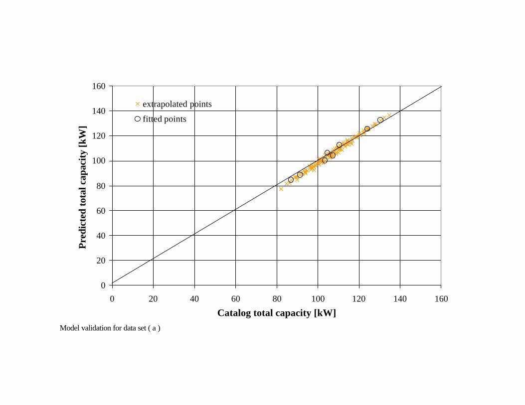
117
Model validation for data set ( a )
0
20
40
60
80
100
120
140
160
0 20 40 60 80 100 120 140 160
Catalog total capacity [kW]
Pre
dict
ed t
otal
cap
acit
y [k
W]
extrapolated points
fitted points

118
Model validation for data set ( a )
0
20
40
60
80
100
120
140
0 20 40 60 80 100 120 140
Catalog sensible capacity [kW]
Pre
dict
ed s
ensi
ble
capa
city
[kW
]
extrapolated points
fitted points

119
Model validation for data set ( b )
0
10
20
30
40
50
0 5 10 15 20 25 30 35 40 45 50
Catalog power draw [kW]
Pre
dict
ed p
ower
dra
w [k
W]
extrapolated points
fitted points

120
Model validation for data set ( b )
0
20
40
60
80
100
120
140
160
0 20 40 60 80 100 120 140 160
Catalog total capacity [kW]
Pre
dict
ed t
otal
cap
acit
y [k
W]
extrapolated points
fitted points

121
Model validation for data set ( b )
0
20
40
60
80
100
120
140
0 20 40 60 80 100 120 140
Catalog sensible capacity [kW]
Pre
dict
ed t
otal
sen
sibl
e [k
W]
extrapolated points
fitted points

122
Model validation for data set ( c )
0
10
20
30
40
50
0 5 10 15 20 25 30 35 40 45 50
Catalog power draw [kW]
Pre
dict
ed p
ower
dra
w [k
W]
extrapolated points
fitted points

123
Model validation for data set ( c )
0
20
40
60
80
100
120
140
160
0 20 40 60 80 100 120 140 160
Catalog total capacity [kW]
Pre
dict
ed to
tal c
apac
ity
[kW
]
extrapolated points
fitted points

124
Model validation for data set ( c )
0
20
40
60
80
100
120
140
0 20 40 60 80 100 120 140
Catalog sensible capacity [kW]
Pre
dict
ed s
ensi
ble
capa
city
[kW
]
extrapolated points
fitted points

125
Model validation for data set ( d )
0
10
20
30
40
50
0 5 10 15 20 25 30 35 40 45 50
Catalog power draw [kW]
Pre
dict
ed p
ower
dra
w [k
W]
extrapolated points
fitted points

126
Model validation for data set ( d )
0
20
40
60
80
100
120
140
160
0 20 40 60 80 100 120 140 160
Catalog total capacity [kW]
Pre
dict
ed to
tal c
apac
ity
[kW
]
extrapolated points
fitted points

127
Model validation for data set ( d )
0
20
40
60
80
100
120
140
0 20 40 60 80 100 120 140
Catalog sensible capacity [kW]
Pre
dict
ed s
ensi
ble
capa
city
[kW
]
extrapolated points
fitted points

128
Appendix B: Model Results for Rooftop Packaged Unit 48 TJ 016 and
48 TJ 024
Data sets used for parameter fitting consisted of eight data points with extreme values
for the volume flow rate, ambient temperature and air entering temperature.
Unit
( 1 ) ( 2 )
48 TJ 016 48 TJ 024
C1 1026 1025
C2 0.5 0.5
C3 1909 1343
Error (sensible) [%] 3.85 6.23
Error (total) [%] 4.78 2.72
C4 987.9 5904
C5 0.5 0.5
C6 31191 14482
Error [%] 8.85 0.164
Validation for 8 fitting points
Error (power) [%] 1.87 4.22
Error (total capacity) [%] 3.00 2.82
Error (sensible capacity) [%] 2.78 1.94
Validation in catalog range
Error (power) [%] 1.55 3.3
Error (total capacity) [%] 2.27 2.07
Error (sensible capacity) [%] 1.87 3.23

129
Model validation for rooftop packaged unit RT 48 TJ 016
0
5
10
15
20
25
0 5 10 15 20 25
Catalog power draw [kW]
Pre
dict
ed p
ower
dra
w [k
W]
extrapolated points
fitted points

130
Model validation for rooftop packaged unit RT 48 TJ 016
0
10
20
30
40
50
60
70
80
0 10 20 30 40 50 60 70 80
Catalog total capacity [kW]
Pre
dict
ed to
tal c
apac
ity
[kW
]
extrapolated points
fitted points

131
Model validation for rooftop packaged unit RT 48 TJ 016
0
10
20
30
40
50
60
70
80
0 10 20 30 40 50 60 70 80
Catalog sensible capacity [kW]
Pre
dict
ed s
ensi
ble
capa
city
[kW
]
extrapolated points
fitted points

132
Model validation for rooftop packaged unit RT 48 TJ 024
0
5
10
15
20
25
30
0 5 10 15 20 25 30
Catalog power draw [kW]
Pre
dict
ed p
ower
dra
w [k
W]
extrapolated points
fitted points

133
Model validation for rooftop packaged unit RT 48 TJ 024
0
20
40
60
80
100
0 20 40 60 80 100
Catalog total capacity [kW]
Pre
dict
ed to
tal c
apac
ity
[kW
]
extrapolated points
fitted points

134
Model validation for rooftop packaged unit RT 48 TJ 024
0
20
40
60
80
100
0 20 40 60 80 100
Catalog sensible capacity [kW]
Pre
dict
ed s
ensi
ble
capa
city
[kW
]
extrapolated points
fitted points

135
Appendix C: EES-code for compressor model (mass flow rate)
"Compressor mass flow rate model" "This program calculates the compressor parameter for the mass flow rate model based on manufacturer's catalog data." $OPENLOOKUP 'parameter.lkt' $SAVELOOKUP 'parameter.lkt' FUNCTION writeLOOKUP(C,DELTAP,N_dot_diagr,V_dot_disp_par, N_cy,nc,unitflag$,capormassflag$,T_sub_diagr,T_sup_diagr,LKT$) LOOKUP(1,'N_dot'):=N_dot_diagr LOOKUP(1,'V_dot_disp'):=V_dot_disp_par LOOKUP(1,'N_cy'):=N_cy LOOKUP(1,'C'):=C LOOKUP(1,'DELTAP'):=DELTAP LOOKUP(1,'nc'):=nc LOOKUP(1,'uc'):=unitflag$ LOOKUP(1,'morc'):=capormassflag$ LOOKUP(1,'T_sub_diagr'):=T_sub_diagr LOOKUP(1,'T_sup_diagr'):=T_sup_diagr LOOKUP(1,'file_comp'):=LKT$ writeLOOKUP:=1 END PROCEDURE capormass(capormassflag$,unitflag$,LKT$,i,h_1r`, h_4r:Cap) IF capormassflag$='Capacity' THEN IF unitflag$='SI' THEN "SI system" Cap:=LOOKUP(LKT$,i,'Capacity')*convert(kW,Btu/hr) ELSE "English system" Cap:=LOOKUP(LKT$,i,'Capacity') ENDIF ELSE IF unitflag$='SI' THEN "SI system" massflowrate:=LOOKUP(LKT$,i,'m_r')*convert(kg/hr,lbm/hr) ELSE "English system" massflowrate:=LOOKUP(LKT$,i,'m_r') ENDIF Cap:=massflowrate*(h_1r`-h_4r) ENDIF END

136
PROCEDURE unitconv(unitflag$,V_dot_disp_diagr,T_sub_diagr, T_sup_diagr:V_dot_disp,T_sub,T_sup) IF unitflag$='SI' THEN "SI system" V_dot_disp := V_dot_disp_diagr*convert(l/s,ft^3/hr) T_sub := T_sub_diagr*1.8 T_sup := T_sup_diagr*1.8 ELSE "English system" V_dot_disp := V_dot_disp_diagr*convert(ft^3/min,ft^3/hr) T_sub := T_sub_diagr T_sup := T_sup_diagr ENDIF END PROCEDURE unitconvarray(unitflag$,T_condenser,T_evaporator: T_cond,T_evap) IF unitflag$='SI' THEN "SI system" T_cond := T_condenser*1.8+32 T_evap := T_evaporator*1.8+32 ELSE "English system" T_cond := T_condenser T_evap := T_evaporator ENDIF END "Capacity or mass flow rate:" DUPLICATE i=1,nc CALL capormass(capormassflag$,unitflag$,LKT$,i,h_1r`[i], h_4r[i]:Cap[i]) END "Unit conversion:" CALL unitconv(unitflag$,V_dot_disp_diagr,T_sub_diagr, T_sup_diagr:V_dot_disp,T_sub,T_sup) DUPLICATE i=1,nc CALL unitconvarray(unitflag$,T_condenser[i],T_evaporator[i]: T_cond[i],T_evap[i]) "Compressor input data:" T_condenser[i]=LOOKUP(LKT$,i,'T_condenser') T_evaporator[i] =LOOKUP(LKT$,i,'T_evaporator') END "Error calculation:" Error_mass =SQRT(SUM(error_mass[i]^2,i=1,nc)/nc) RMS_mass=SQRT(SUM((m_r[i]-m_r_calc[i])^2,i=1,nc)/nc) DUPLICATE i=1,nc Error_mass[i]=(m_r[i]-m_r_calc[i])/m_r_mean END m_r_mean=SUM(m_r[i],i=1,nc)/nc

137
"Data range:" lower_m=MIN(m_r[1..nc])/m_r_mean upper_m=MAX(m_r[1..nc])/m_r_mean "Gas constant:" R_m=1.986 R=R_m/M_R22 M_R22=MOLARMASS(R22) "Calculated mass flow rate:" DUPLICATE i=1,nc m_r_calc[i]=(1+C-C*((P_r_cond[i]/P_r_suction[i]))^(1/k[i]))* V_dot_disp/v_suction[i] "Volumetric efficiencies:" eta_V[i]=m_r_calc[i]*v_suction[i]/V_dot_disp eta_V_measured[i]=m_r[i]*v_suction[i]/V_dot_disp "Capacity and mass flow rate:" Cap[i]=m_r[i]*(h_1r`[i]-h_4r[i]) "Polytropic exponent:" k[i]=SPECHEAT(R22,T=T_r_suction[i],P=P_r_suction[i])/(SPECHEAT(R22,T=T_r_suction[i],P=P_r_suction[i])-R) "Enthalpies:" h_1r[i]=ENTHALPY(R22,P=P_1r[i], x=1) h_1r`[i]=ENTHALPY(R22,P=P_1r`[i], T=T_1r`[i]) h_3r[i]=ENTHALPY(R22,P=P_3r[i], x=0) h_3r`[i]=ENTHALPY(R22,P=P_3r[i],T=T_3r`[i]-0.001) h_4r[i]=h_3r`[i] "Temperatures:" T_1r[i]=T_evap[i] T_1r`[i]=T_evap[i]+T_sup T_r_suction[i]=T_evap[i]+T_sup T_3r[i]=T_cond[i] T_3r`[i]=T_cond[i]-T_sub T_4r[i]=T_evap[i] "Pressures:" P_r_cond[i]=PRESSURE(R22,T=T_cond[i],x=0) P_r_evap[i]=PRESSURE(R22,T=T_evap[i],x=1) P_r_suction[i]=P_r_evap[i]*(1-DELTAP) P_dis\P_suc[i]=P_r_cond[i]/P_r_evap[i] P_1r[i]=P_r_evap[i] P_1r`[i]=P_r_evap[i] P_2r[i]=P_r_cond[i] P_2rs[i]=P_r_cond[i] P_3r[i]=P_r_cond[i] P_3r`[i]=P_r_cond[i] P_4r[i]=P_r_evap[i] "Specific volumes:" v_suction[i]=VOLUME(R22,T=T_1r`[i],P=P_r_suction[i])

138
"Writes data to LOOKUP table:" dummy[i]=writeLOOKUP(C,DELTAP,N_dot_diagr,V_dot_disp_par,N_cy,nc,unitflag$,capormassflag$,T_sub_diagr,T_sup_diagr,LKT$) END V_dot_disp_par=V_dot_disp*convert(ft^3/hr,ft^3/min)

139
Appendix D: EES-code for compressor model (power)
"Compressor power model" $OPENLOOKUP 'parameter.lkt' $SAVELOOKUP 'parameter.lkt' FUNCTION writeLOOKUP(a,b) LOOKUP(1,'a'):=a LOOKUP(1,'b'):=b writeLOOKUP:=1 END PROCEDURE capormass(capormassflag$,unitflag$,LKT$,i,h_1r`, h_4r:Cap) IF capormassflag$='Capacity' THEN IF unitflag$='SI' THEN "SI system" Cap:=LOOKUP(LKT$,i,'Capacity')*convert(kW,Btu/hr) ELSE "English system" Cap:=LOOKUP(LKT$,i,'Capacity') ENDIF ELSE IF unitflag$='SI' THEN "SI system" massflowrate:=LOOKUP(LKT$,i,'m_r')*convert(kg/hr,lbm/hr) ELSE "English system" massflowrate:=LOOKUP(LKT$,i,'m_r') ENDIF Cap:=massflowrate*(h_1r`-h_4r) ENDIF END PROCEDURE unitconv(unitflag$,V_dot_disp,T_sub_diagr, T_sup_diagr:V_dot_disp_diagr,T_sub,T_sup) IF unitflag$='SI' THEN "SI system" V_dot_disp_diagr:=V_dot_disp*convert(ft^3/hr,l/s) T_sub:=T_sub_diagr*1.8 T_sup:=T_sup_diagr*1.8 ELSE "English system" V_dot_disp_diagr:=V_dot_disp*convert(ft^3/hr,ft^3/min) T_sub:=T_sub_diagr T_sup:=T_sup_diagr ENDIF END

140
PROCEDURE unitconvarray(unitflag$,T_condenser,T_evaporator: T_cond,T_evap) IF unitflag$='SI' THEN "SI system" T_cond:=T_condenser*1.8+32 T_evap:=T_evaporator*1.8+32 ELSE "English system" T_cond:=T_condenser T_evap:=T_evaporator ENDIF END "Reads information from the parameter table:" LKT$=LOOKUP$(1,'file_comp') nc=LOOKUP(1,'nc') unitflag$=LOOKUP$(1,'uc') capormassflag$=LOOKUP$(1,'morc') "Capacity or mass flow rate:" DUPLICATE i=1,nc CALL capormass(capormassflag$,unitflag$,LKT$,i,h_1r`[i], h_4r[i]:Cap[i]) END "Unit conversion:" CALL unitconv(unitflag$,V_dot_disp,T_sub_diagr, T_sup_diagr:V_dot_disp_diagr,T_sub,T_sup) DUPLICATE i=1,nc CALL unitconvarray(unitflag$,T_condenser[i],T_evaporator[i]: T_cond[i],T_evap[i]) "Compressor input data:" T_condenser[i]=LOOKUP(LKT$,i,'T_condenser') T_evaporator[i]=LOOKUP(LKT$,i,'T_evaporator') Power[i]=LOOKUP(LKT$,i,'Power') END V_dot_disp =LOOKUP(1,'V_dot_disp')*convert(ft^3/min,ft^3/hr) N_dot_diagr=LOOKUP(1,'N_dot') N_dot=N_dot_diagr*convert(1/min,1/hr) N_cy=LOOKUP(LKT$,1,'N_cy') C=LOOKUP(1,'C') DELTAP=LOOKUP(1,'DELTAP') "Rating conditions:" T_sub_diagr=LOOKUP(1,'T_sub_diagr') "F, Subcooling" T_sup_diagr=LOOKUP(1,'T_sup_diagr') "F, Return gas temperature" "Error calculation:" Error_mass =SQRT(SUM(Error_mass[i]^2,i=1,nc)/nc) RMS_mass=SQRT(SUM((m_r[i]-m_r_calc[i])^2,i=1,nc)/nc)

141
Error_power=SQRT(SUM(Error_power[i]^2,i=1,nc)/nc) RMS_power=SQRT(SUM((Power[i]-P_com_calc[i])^2,i=1,nc)/nc) DUPLICATE i=1,nc Error_mass[i]=(m_r[i]-m_r_calc[i])/m_r_mean Error_power[i]=(Power[i]-P_com_calc[i])/P_com_mean END m_r_mean=SUM(m_r[i],i=1,nc)/nc P_com_mean=SUM(Power[i],i=1,nc)/nc "Data range:" lower_m=MIN(m_r[1..nc])/m_r_mean upper_m=MAX(m_r[1..nc])/m_r_mean lower_P=MIN(Power[1..nc])/P_com_mean upper_P=MAX(Power[1..nc])/P_com_mean "Gas constant:" R_m=1.986 R=R_m/M_R22 M_R22=MOLARMASS(R22) "Calculated mass flow rate:" DUPLICATE i=1,nc m_r_calc[i]=(1+C-C*((P_r_cond[i]/P_r_suction[i]))^(1/k[i]))* V_dot_disp/v_suction[i] "Volumetric efficiency:" eta_V[i]=m_r_calc[i]*v_suction[i]/V_dot_disp eta_V_measured[i]=m_r[i]*v_suction[i]/V_dot_disp "Capacity and mass flow rate:" Cap[i]=m_r[i]*(h_1r`[i]-h_4r[i]) "Power:" P_com[i]=m_r[i]*(h_2r[i]-h_1r`[i]) P_com[i]=P_com_calc[i]*eta_comb[i]*convert(kW,Btu/hr) P_com_calc[i]*eta_comb[i]=convert(W,kW)*m_r_calc[i]*convert(lbm/hr,kg/s)*(k[i]/(k[i]-1))*P_r_suction[i]*convert(atm,Pa)*(v_suction[i]*convert(ft^3/lbm,m^3/kg))*((P_2r[i]/P_r_suction[i])^((k[i]-1)/k[i])-1) eta_comb[i]=a+b/P_r_evap[i] "Polytropic exponent:" k[i]=SPECHEAT(R22,T=T_r_suction[i],P=P_r_suction[i])/(SPECHEAT(R22,T=T_r_suction[i],P=P_r_suction[i])-R) "Isentropic efficiency:" eta_S[i]=m_r[i]*(h_2rs[i]-h_1r`[i])/P_com[i] "Entropies:" s_1r`[i]=ENTROPY(R22,P=P_1r`[i], T=T_1r`[i]) s_2rs[i]=s_1r`[i] "Enthalpies:" h_1r[i]=ENTHALPY(R22,P=P_1r[i], x=1) h_1r`[i]=ENTHALPY(R22,P=P_1r`[i], T=T_1r`[i]) h_2rs[i]=ENTHALPY(R22,P=P_2rs[i],s=s_2rs[i])

142
h_3r[i]=ENTHALPY(R22,P=P_3r[i], x=0) h_3r`[i]=ENTHALPY(R22,P=P_3r`[i],T=T_3r`[i]-0.001) h_4r[i]=h_3r`[i] "Temperatures:" T_1r[i]=T_evap[i] T_1r`[i]=T_evap[i]+T_sup T_r_suction[i]=T_evap[i]+T_sup T_3r[i]=T_cond[i] T_3r`[i]=T_cond[i]-T_sub T_4r[i]=T_evap[i] "Pressures:" P_r_cond[i]=PRESSURE(R22,T=T_cond[i],x=0) P_r_evap[i]=PRESSURE(R22,T=T_evap[i],x=1) P_r_suction[i]=P_r_evap[i]*(1-DELTAP) P_dis\P_suc[i]=P_r_cond[i]/P_r_evap[i] P_1r[i]=P_r_evap[i] P_1r`[i]=P_r_evap[i] P_2r[i]=P_r_cond[i] P_2rs[i]=P_r_cond[i] P_3r[i]=P_r_cond[i] P_3r`[i]=P_r_cond[i] P_4r[i]=P_r_evap[i] "Specific volumes:" v_suction[i]=VOLUME(R22,T=T_1r`[i],P=P_r_suction[i]) "Writes data in LOOKUP table:" dummy[i]=writeLOOKUP(a,b) "Unit conversion for plot windows:" m_r_SI[i]=m_r[i]*convert(lbm/hr,kg/hr) m_r_calc_SI[i]=m_r_calc[i]*convert(lbm/hr,kg/hr) END

143
Appendix E: EES-code for vapor compression cycle
“Calculates thermodynamic state points and rate equations for the assumed vapor compression cycle” $OPENLOOKUP 'parameter.lkt' $SAVELOOKUP 'parameter.lkt' PROCEDURE unitconvarray1(unitflag$,Q_evap_cat,SHC_cat, T_db_amb_cat,T_db_1_cat,T_wb_1_cat:Q_evap,SHC,T_db_amb,T_db_1,T_wb_1) IF unitflag$='SI' THEN "SI system" Q_evap:=Q_evap_cat*convert(kW,Btu/s) SHC:=SHC_cat*convert(kW,Btu/s) T_db_amb:=T_db_amb_cat*1.8+32 T_db_1:=T_db_1_cat*1.8+32 T_wb_1:=T_wb_1_cat*1.8+32 ELSE "English system" Q_evap:=Q_evap_cat*convert(MBtu/hr,Btu/s) SHC:SHC_cat*convert(MBtu/hr,Btu/s) T_db_amb:=T_db_amb_cat T_db_1:=T_db_1_cat T_wb_1:=T_wb_1_cat ENDIF END PROCEDURE unitconvarray2(unitflag$,V_circ_cat,V_cat_cat, A_evap_cat,Powerdraw_comp_cat:V_circ,V_cat,A_evap, Powerdraw_comp) IF unitflag$='SI' THEN "SI system" V_circ:=V_circ_cat*convert(l/s,ft^3/min) V_cat:=V_cat_cat*convert(l/s,ft^3/min) A_evap:=A_evap_cat*convert(m^2,ft^2) Powerdraw_comp:=Powerdraw_comp_cat ELSE "English system" V_circ:=V_circ_cat V_cat:=V_cat_cat A_evap:=A_evap_cat Powerdraw_comp:=Powerdraw_comp_cat ENDIF END FUNCTION writeLOOKUP1(i,length,CT,ST,vel,EDB,EWB,LDB, LWB,T_air_in,T_air_out,T_cond,m_r,m_a,Q_cond,N_comp,A_evap) LOOKUP(1,'Length'):=length

144
LOOKUP(i,'CT'):=CT LOOKUP(i,'ST'):=ST LOOKUP(i,'vel') :=vel LOOKUP(i,'EDB') :=EDB LOOKUP(i,'EWB') :=EWB LOOKUP(i,'LDB') :=LDB LOOKUP(i,'LWB') :=LWB LOOKUP(i,'T_air_in') :=T_air_in LOOKUP(i,'T_air_out'):=T_air_out LOOKUP(i,'T_cond'):=T_cond LOOKUP(i,'m_r') :=m_r LOOKUP(i,'m_a') :=m_a LOOKUP(i,'Q_cond'):=Q_cond LOOKUP(1,'N_comp'):=N_comp LOOKUP(i,'A_evap'):=A_evap writeLOOKUP1:=1 END FUNCTION writeLOOKUP2(m,rooftop$,unitflag$) LOOKUP(1,'nu'):=m LOOKUP(1,'file_unit'):=rooftop$ LOOKUP(1,'uu'):=unitflag$ writeLOOKUP2:=1 END n=1 "Writes information to the parameter table:" DUPLICATE i=n,m dummy1[i]=writeLOOKUP1(i,length,T_3r[i],T_1r[i],FPM[i], T_db_1[i],T_wb_1[i],T_db_2[i],T_wb_2[i],T_db_amb[i],T_db_co[i],T_3r[i],m_r[i],m_cond_a[i],Q_cond[i],N_comp,A_evap[i]) END dummy2=writeLOOKUP2(m,rooftop$,unitflag$) "Knowns from catalog:" P_amb=14.7 DUPLICATE i=n,m CALL unitconvarray1(unitflag$,Q_evap_cat[i],SHC_cat[i], T_db_amb_cat[i],T_db_1_cat[i],T_wb_1_cat[i]:Q_evap[i],SHC[i], T_db_amb[i],T_db_1[i],T_wb_1[i]) CALL unitconvarray2(unitflag$,V_circ_cat[i],V_cat_cat[i], A_evap_cat[i],Powerdraw_comp_cat[i]:V_circ[i],V_cat[i], A_evap[i],Powerdraw_comp[i]) END DUPLICATE i=n,m Q_evap_cat[i]=LOOKUP(Rooftop$,i,#Q_tot) SHC_cat[i] =LOOKUP(Rooftop$,i,#SHC)

145
T_db_amb_cat[i] =LOOKUP(Rooftop$,i,#TDB_amb) T_db_1_cat[i]=LOOKUP(Rooftop$,i,#TDB_i) T_wb_1_cat[i]=LOOKUP(Rooftop$,i,#TWB_i) V_circ_cat[i]=LOOKUP(Rooftop$,i,#V_air) V_cat_cat[i]=LOOKUP(1,#V_dot_cond_fan) Powerdraw_comp_cat[i]=LOOKUP(Rooftop$,i,#Power) SHR[i]=SHC[i]/Q_evap[i] END A_evap_cat =A_evap_cat[1] DUPLICATE i=n,m-1 A_evap_cat[i]=A_evap_cat[i+1] END "Evaporator (air-side):" DUPLICATE i=n,m Q_evap[i]=m_a[i]*(h_1[i]-h_2[i]) m_a[i]=rho_1[i]*V_a[i] rho_1[i]=DENSITY(AirH2O,T=T_db_1[i],B=T_wb_1[i],P=P_1[i]) w_1[i]=HUMRAT(AirH2O,T=T_db_1[i],P=P_amb,B=T_wb_1[i]) w_2[i]=HUMRAT(AirH2O,T=T_db_2[i],P=P_amb,B=T_wb_2[i]) h_1[i]=ENTHALPY(AirH2O,T=T_db_1[i],P=P_1[i],w=w_1[i]) h_2[i]=ENTHALPY(AirH2O,T=T_db_2[i],P=P_2[i],w=w_2[i]) V_a[i]=V_circ[i]*convert(ft^3/min, ft^3/s) P_1[i]=P_amb Q_evap_sen[i]=Q_evap[i]*SHR[i] Q_evap_sen[i]=m_a[i]*c_p1[i]*dT[i] c_p1[i]=SPECHEAT(AirH2O,T=T_mean_evap_a[i], B=T_wb_mean_evap_a[i],P=P_1[i]) dT[i]=T_db_1[i]-T_db_2[i] T_mean_evap_a[i]=(T_db_1[i]+T_db_2[i])/2 T_wb_mean_evap_a[i]=(T_wb_1[i]+T_wb_2[i])/2 P_2[i]=P_1[i] FPM[i]=V_circ[i]/A_evap[i] END Length=SQRT(A_evap[n]*convert(ft^2,in^2)) "Condenser (air-side):" DUPLICATE i=n,m Q_cond[i]=m_cond_a[i]*c_P_cond[i]*(T_db_co[i]-T_db_amb[i]) c_p_cond[i]=SPECHEAT(Air,T=T_mean_cond_a[i]) m_cond_a[i]=V_cond_a[i]/vol_cond_a[i] V_cond_a[i]=V_cat[i]*convert(ft^3/min,ft^3/s) vol_cond_a[i]=VOLUME(Air,T=T_db_amb[i],P=P_amb) T_mean_cond_a[i]=(T_db_amb[i]+T_db_co[i])/2 END "Compressor data:" N_dot=LOOKUP(1,'N_dot')*convert(1/min,1/hr) V_dot_disp =LOOKUP(1,'V_dot_disp')*convert(1/min,1/hr)

146
a=LOOKUP(1,'a') b=LOOKUP(1,'b') C=LOOKUP(1,'C') DELTAP=LOOKUP(1,'DELTAP') V_disp=V_dot_disp/N_dot DUPLICATE i=n,m P_r_suction[i]=P_r_evap[i]*(1-DELTAP) “Specific volumes:" v_suction[i]=VOLUME(R22,T=T_1r[i],P=P_r_suction[i]-0.1) "Polytropic exponent:" k[i]=SPECHEAT(R22,T=T_1r[i],P=P_r_suction[i]-0.1)/(SPECHEAT (R22,T=T_1r[i],P=P_r_suction[i]-0.1)-R) END "Calculation of the power:" DUPLICATE i=n,m P_comp[i]=N_comp*(1-k_loss)*P_com_calc[i]*eta_comb[i] *convert(W,Btu/s) P_com_calc[i]*eta_comb[i]=m_r_calc[i]*convert(lbm/hr,kg/s) *(k[i]/(k[i]-1))*P_r_suction[i]*convert(psia,Pa)*(v_suction[i] *convert(ft^3/lbm,m^3/kg))*((P_r_cond[i]/P_r_suction[i]) ^((k[i]-1)/k[i])-1) eta_comb[i]=a+b/(P_r_evap[i]*convert(psia,atm)) "Volumetric efficiency:" eta_V[i]=m_r_calc[i]*v_suction[i]/V_dot_disp "Calculated mass flow rate:" m_r_calc[i]=(1+C-C*((P_r_cond[i]/P_r_suction[i]))^(1/k[i])) *V_dot_disp/v_suction[i] "Output of compressor model:" Powerdraw_comp[i]=Power_r_comp[i]*convert(Btu/s,kW) Power_r_comp[i] =N_comp*P_com_calc[i]*convert(W,Btu/s) Power_r_comp_kW[i]=N_comp*P_com_calc[i]*convert(W,kW) m_r[i]=N_comp*m_r_calc[i]*convert(lbm/hr,lbm/s) END "Ideal gas constant:" R_m=1.986 R=R_m/M_R22 M_R22=MOLARMASS(R22) "Refrigeration cycle:" DUPLICATE i=n,m "Energy balance:" Q_evap[i]+P_comp[i]=Q_cond[i] "Heat transfer at the evaporator:" Q_evap[i]=m_r[i]*(h_1r[i]-h_4r[i]) "Power relationships for the compressor:" P_comp[i]=m_r[i]*(h_2r[i]-h_1r[i]) "Enthalpies:"

147
h_1r[i]=ENTHALPY(R22,T=T_1r[i],x=1) h_2r`[i]=ENTHALPY(R22,T=T_3r[i],x=1) Q_cond_real[i]=m_r[i]*(h_2r`[i]-h_3r[i]) h_3r[i]=ENTHALPY(R22,T=T_3r[i],x=0) h_4r[i]=h_3r[i] "Temperatures:" T_2r[i]=TEMPERATURE(R22,h=h_2r[i],P=P_r_cond[i]) T_2r`[i]=TEMPERATURE(R22,P=P_r_cond[i],x=1) T_4r[i]=TEMPERATURE(R22,h=h_4r[i],P=P_r_evap[i]) "Pressures:" P_r_cond[i]=PRESSURE(R22,T=T_3r[i],x=0) P_r_evap[i]=PRESSURE(R22,T=T_1r[i],x=1) END

148
Appendix F: EES-code for direct expansion coil model
“Calculates the heat exchanger parameters used for the direct expansion coil model” $OPENLOOKUP 'parameter.lkt' $SAVELOOKUP 'parameter.lkt' PROCEDURE DryCoil (Length,m_a,m_ref,EDB,EWB,CT,ST,C_1,C_2,C_3: Q_dry,LDB_dry,LWB_dry,hA_o_dry,hA_i_dry) LDB_dry:=EDB "assumed leaving dry bulb temperature" w_i:=HUMRAT(AirH2O,T=EDB,B=EWB,P=14.7) "entering humidity ratio" 10: MDB_dry:=(EDB+LDB_dry)/2 "mean dry bulb temperature" MST_dry:=ST+(MDB_dry-ST)/10 "mean surface temperature" cp_b_a_dry:=SPECHEAT(Air,T=MDB_dry) "specific heat" mu_b_a_dry:=VISCOSITY(Air,T=MDB_dry) "mean bulk dynamic viscosity of air" k_b_a_dry:=CONDUCTIVITY(Air,T=MDB_dry) "mean bulk thermal conductivity of air" cp_s_a_dry:=SPECHEAT(Air,T=MST_dry) "specific heat" mu_s_a_dry:=VISCOSITY(Air,T=MST_dry) "dynamic viscosity of air at mean surface temperature" k_s_a_dry:=CONDUCTIVITY(Air,T=MST_dry) "thermal conductivity of air at mean surface temperature" P_cond:=PRESSURE(R22,T=CT,x=0) "condenser pressure" P_evap:=PRESSURE(R22,T=ST,x=0) "evaporator pressure" mu_ref_1:=VISCOSITY(R22,T=ST,P=P_evap+0.001) "dynamic viscosity of liquid refrigerant" k_ref_1:=CONDUCTIVITY(R22,T=ST,P=P_evap+0.001) "thermal conductivity of liquid refrigerant" h_in:=ENTHALPY(R22,T=CT,x=0) "specific enthalpy of inlet refrigerant" h_out:=ENTHALPY(R22,T=ST,x=1) "specific enthalpy of outlet refrigerant" x_in:=QUALITY(R22,h=h_in,T=ST) "inlet quality of refrigerant" h_fg:=ENTHALPY(R22,T=ST,x=1)-ENTHALPY(R22,T=ST,x=0) "latent heat of fusion" "Overall heat transfer coefficient-area products (dry-coil)"

149
hA_o_dry:=C_1*(m_a/mu_b_a_dry)^C_2*(mu_b_a_dry*cp_b_a_dry/k_b_a_dry)^0.36*((mu_b_a_dry*cp_b_a_dry/k_b_a_dry)/(mu_s_a_dry*cp_s_a_dry/k_s_a_dry))^0.25*k_b_a_dry"Btu/hr-ft" hA_i_dry:=C_3*k_ref_1*((m_ref/mu_ref_1)*(1-x_in)*h_fg)^0.45 UA_tot_dry:=1/(1/hA_i_dry+1/hA_o_dry) "Btu/hr-F" "Capacitance rates" C_min:=m_a*cp_b_a_dry "minimum capacitance rate" NTU_dry:=UA_tot_dry/C_min "totally dry coil NTU's" epsilon_dry:=1-exp(-NTU_dry) "effectiveness of dry portion coil" Q_dry:=epsilon_dry*C_min*(EDB-ST) "energy transfer rate for a totally dry coil" LDB_new_dry:=EDB-Q_dry/(m_a*cp_b_a_dry) "air outlet temperature" IF (abs(LDB_dry-LDB_new_dry)>=0.1) THEN LDB_dry:=LDB_new_dry goto 10 ENDIF LWB_dry:=WetBulb(AirH2O,T=LDB_dry,P=14.7,W=w_i) "wet bulb temperature of air leaving dry portion of coil" END PROCEDURE WetCoil (Length,m_a,m_ref,EDB,EWB,CT,ST,FPM,C_1,C_2, C_3:Q_wet,LDB_wet,LWB_wet,hA_o_wet,hA_i_wet) DP_i=DewPoint(AirH2O,T=EDB,B=EWB,P=14.7) "entering dewpoint" LDB_wet:=EWB-20 "assumed leaving dry bulb temperature" w_i:=HUMRAT(AirH2O,T=EDB,B=EWB,P=14.7) "entering humidity ratio" 20: MDB_wet:=(EDB+LDB_wet)/2 "mean dry bulb temperature for a totally wet coil" MST_wet:=ST+(MDB_wet-ST)/10 "mean surface temperature for a totally wet coil" cp_sat:=(ENTHALPY(AirH2O,T=DP_i,R=1,P=14.7)-ENTHALPY(AirH2O,T=ST,R=1,P=14.7))/(DP_i-ST) "saturation specific heat" h_a_i:=ENTHALPY(AirH2O,T=EDB,B=EWB,P=14.7) "specIFic enthalpy of entering air" h_ref_sat_i:=ENTHALPY(AirH2O,T=ST,R=1,P=14.7) "saturation specific enthalpy at suction temperature" cp_b_a_wet:=SPECHEAT(Air,T=MDB_wet) "specific heat" mu_b_a_wet:=VISCOSITY(Air,T=MDB_wet) "mean bulk dynamic viscosity of air" k_b_a_wet:=CONDUCTIVITY(Air,T=MDB_wet) "mean bulk thermal conductivity of air" cp_s_a_wet:=SPECHEAT(Air,T=MST_wet) "specific heat"

150
mu_s_a_wet:=VISCOSITY(Air,T=MST_wet) "dynamic viscosity of air at mean surface temperature" k_s_a_wet:=CONDUCTIVITY(Air,T=MST_wet) "thermal conductivity of air at mean surface temperature" P_cond:=PRESSURE(R22,T=CT,x=0) "condenser pressure" P_evap:=PRESSURE(R22,T=ST,x=0) "evaporator pressure" mu_ref_1:=VISCOSITY(R22,T=ST,P=P_evap+0.001)"dynamic viscosity of liquid refrigerant" k_ref_1:=CONDUCTIVITY(R22,T=ST,P=P_evap+0.001) "thermal conductivity of liquid refrigerant" h_in:=ENTHALPY(R22,T=CT,x=0) " specific enthalpy of inlet refrigerant" h_out:=ENTHALPY(R22,T=ST,x=1) "specific enthalpy of outlet refrigerant" x_in:=QUALITY(R22,h=h_in,T=ST) "inlet quality of refrigerant" h_fg:=ENTHALPY(R22,T=ST,x=1)-ENTHALPY(R22,T=ST,x=0) "latent heat of fusion" "Overall heat transfer coefficient-area products (wet-coil)" C_f:=0.626*FPM^0.101 "air side convection coefficient correction factor for a totally wet coil" hA_o_wet:=C_f*C_1*(m_a/mu_b_a_wet)^C_2*(mu_b_a_wet*cp_b_a_wet /k_b_a_wet)^0.36*((mu_b_a_wet*cp_b_a_wet/k_b_a_wet) /(mu_s_a_wet*cp_s_a_wet/k_s_a_wet))^0.25*k_b_a_wet "Btu/hr-ft" hA_i_wet:=C_3*k_ref_1*((m_ref/mu_ref_1)*(1-x_in)*h_fg)^0.45 UA_h:=1/(cp_sat/hA_i_wet+cp_b_a_wet/hA_o_wet) "Btu/hr-ft" capAirWet:=m_a NTU_wet:=UA_h/m_a epsilon_wet:=1-exp(-NTU_wet) "effectiveness of wet coil" Qmax_wet:=m_a*abs(h_a_i-h_ref_sat_i) h_a_o:=h_a_i-epsilon_wet*Qmax_wet/capAirWet h_ref_sat_o:=h_ref_sat_i R_i:=1/hA_i_wet R_o:=1/hA_o_wet Rratio:=R_i/(R_i+cp_b_a_wet/cp_sat*R_o) h_s_sat_i:=h_ref_sat_o+Rratio*(h_a_i-h_ref_sat_o) h_s_sat_o:=h_ref_sat_i+Rratio*(h_a_o-h_ref_sat_i) T_s_i:=TEMPERATURE(AirH2O,P=14.7,R=1,h=h_s_sat_i) Q_wet:=m_a*(h_a_i-h_a_o) capAir:=m_a*(SpecHeat(Air,T=MDB_wet)+w_i*SpecHeat(H2O, T=MDB_wet)) capAir_2:=m_a*SPECHEAT(AirH2O,T=MDB_wet,P=14.7,w=w_i) NTU:=hA_o_wet/capAir epsilon:=1-exp(-NTU) h_sat_cond:=h_a_i-(h_a_i-h_a_o)/epsilon

151
T_cond:=TEMPERATURE(AirH2O,P=14.7,R=1,H=h_sat_cond) LDB_new_wet:=EDB-(EDB-T_cond)*epsilon IF (abs(LDB_wet-LDB_new_wet)>=0.1) THEN LDB_wet:=LDB_new_wet goto 20 ENDIF w_o:=(h_a_o-(ENTHALPY(Air,T=LDB_wet)-ENTHALPY(Air,T=0)))/ENTHALPY(Water,T=LDB_wet,x=1) LWB_wet:=WETBULB(AirH2O,T=LDB_wet,P=14.7,w=w_o) "F; wet bulb temperature of air leaving wet portion of coil" END PROCEDURE Compare(EDB, EWB, ST, Q_dry, LDB_dry, LWB_dry, hA_o_dry, hA_i_dry, Q_wet, LDB_wet, LWB_wet, hA_o_wet, hA_i_wet: Q_calc, LDB_calc, LWB_calc, hA_o_calc, hA_i_calc) DP_i=DEWPOINT(AirH2O,T=EDB,B=EWB,P=14.7) "F; entering dew point" IF (DP_i<=ST) THEN Q_calc:=Q_dry LDB_calc:=LDB_dry LWB_calc:=LWB_dry hA_o_calc:=hA_o_dry hA_i_calc:=hA_i_dry ELSE Ts_i=(EDB+ST)/2 IF (DP_i<=Ts_i) THEN IF (Q_dry>Q_wet) THEN Q_calc:=Q_dry LDB_calc:=LDB_dry LWB_calc:=LWB_dry hA_o_calc:=hA_o_dry hA_i_calc:=hA_i_dry ELSE Q_calc:=Q_wet LDB_calc:=LDB_wet LWB_calc:=LWB_wet hA_o_calc:=hA_o_wet hA_i_calc:=hA_i_wet ENDIF ELSE Q_calc:=Q_wet LDB_calc:=LDB_wet LWB_calc:=LWB_wet hA_o_calc:=hA_o_wet hA_i_calc:=hA_i_wet ENDIF ENDIF

152
END FUNCTION writeLOOKUP(C_1,C_2,C_3) LOOKUP(1,'C_1'):=C_1 LOOKUP(1,'C_2'):=C_2 LOOKUP(1,'C_3'):=C_3 writeLOOKUP:=1 END n=LOOKUP(1,'nu') DUPLICATE i=1,n EDB[i]=LOOKUP(i,#EDB) "entering air dry bulb temperature" EWB[i]=LOOKUP(i,#EWB) "entering air wet bulb temperature" CT[i]=LOOKUP(i,#CT) "condensing temperature" ST[i]=LOOKUP(i,#ST) "suction temperature" FPM[i]=LOOKUP(i,#vel) "air velocity" LDB[i]=LOOKUP(i,#LDB) "leaving air dry bulb temperature" LWB[i]=LOOKUP(i,#LWB) "leaving air wet bulb temperature" "Catalog performance" h_i[i]=ENTHALPY(AirH2O,T=EDB[i],B=EWB[i],P=14.7) h_o[i]=ENTHALPY(AirH2O,T=LDB[i],B=LWB[i],P=14.7) m_a[i]=rho_std[i]*Area*FPM[i]*60 Q_act[i]=m_a[i]*(h_i[i]-h_o[i]) h_ref_i[i]=ENTHALPY(R22,T=CT[i],X=0) h_ref_o[i]=ENTHALPY(R22,T=ST[i],X=1) Q_act[i]=m_ref[i]*(h_ref_o[i]-h_ref_i[i]) "Coil models" Call DryCoil (Length,m_a[i],m_ref[i],EDB[i],EWB[i],CT[i],ST[i] ,C_1,C_2,C_3:Q_dry[i],LDB_dry[i],LWB_dry[i],hA_o_dry[i], hA_i_dry[i]) Call WetCoil (Length,m_a[i],m_ref[i],EDB[i],EWB[i],CT[i], ST[i],FPM[i],C_1,C_2,C_3:Q_wet[i],LDB_wet[i],LWB_wet[i], hA_o_wet[i],hA_i_wet[i]) Call Compare (EDB[i],EWB[i],ST[i],Q_dry[i],LDB_dry[i],LWB_dry[i], hA_o_dry[i],hA_i_dry[i],Q_wet[i],LDB_wet[i],LWB_wet[i], hA_o_wet[i],hA_i_wet[i]:Q_calc[i],LDB_calc[i],LWB_calc[i], hA_o_calc[i],hA_i_calc[i]) END Length=LOOKUP(1,#length) Area=length^2*convert(in^2,ft^2) DUPLICATE i=1,n rho_std[i]=DENSITY(Air,T=EDB[i],P=14.7) Q_evap[i]=Q_act[i]*convert(Btu/hr,Btu/s) Q_evap_calc[i]=Q_calc[i]*convert(Btu/hr,Btu/s) Error_evap_mean[i]=(Q_evap[i]-Q_evap_calc[i])/Q_evap_mean

153
END Q_evap_mean=SUM(Q_evap[i],i=1,n)/(n) Error_evap=SQRT(SUM((Error_evap_mean[i])^2,i=1,n)/(n)) RMS_evap=SQRT(SUM((Q_evap[i]-Q_evap_calc[i])^2,i=1,n)/n) lower_Q=MIN(Q_evap[1..n])/Q_evap_mean upper_Q=MAX(Q_evap[1..n])/Q_evap_mean DUPLICATE i=1,n “Calculation of plot variables:" Q_evaporator[i] =Q_evap[i]*convert(Btu/s,MBtu/hr) Q_evaporator_calc[i] =Q_evap_calc[i]*convert(Btu/s,MBtu/hr) Q_evaporator_SI[i]=Q_evap[i]*convert(Btu/s,kW) Q_evaporator_calc_SI[i]=Q_evap_calc[i]*convert(Btu/s,kW) END dummy=writeLOOKUP(C_1,C_2,C_3) DUPLICATE i=1,n T_db_mean[i]=(EDB[i]+LDB[i])/2 T_wb_mean[i]=(EWB[i]+LWB[i])/2 c_p_mean[i]=SPECHEAT(AirH2O,T=T_db_mean[i],B=T_wb_mean[i], p=14.7) SHC[i]=m_a[i]*c_p_mean[i]*(EDB[i]-LDB[i]) *convert(Btu/hr,Btu/s) T_db_mean_calc[i]=(EDB[i]+LDB_calc[i])/2 T_wb_mean_calc[i]=(EWB[i]+LWB_calc[i])/2 c_p_mean_calc[i]=SPECHEAT(AirH2O,T=T_db_mean_calc[i], B=T_wb_mean_calc[i],p=14.7) SHC_calc[i]=m_a[i]*c_p_mean_calc[i]*(EDB[i]-LDB_calc[i]) *convert(Btu/hr,Btu/s) Error_SHC_mean[i]=(SHC[i]-SHC_calc[i])/SHC_mean END SHC_mean=SUM(SHC[i],i=1,n)/(n) Error_SHC=SQRT(SUM((Error_SHC_mean[i])^2,i=1,n)/(n)) Error_total=(Error_SHC+Error_evap)/2

154
Appendix G: EES-code for 3-parameter condensing coil model
“Calculates the heat exchanger parameters used for the 3-parameter condensing coil model” $OPENLOOKUP 'parameter.lkt' $SAVELOOKUP 'parameter.lkt' PROCEDURE CondCoil(T_air_in,T_air_out,T_cond,m_r,m_a,C_4,C_5, C_6:hA_i,hA_o,Q_calc,epsilon) m_r:=m_r*3600 m_a:=m_a*3600 P_cond:=PRESSURE(R22,T=T_cond,x=1) c_P:=SPECHEAT(R22,T=T_cond,P=P_cond+0.001) k_r:=CONDUCTIVITY(R22,T=T_cond,x=0) mu_r:=VISCOSITY(R22,T=T_cond,x=0) rho_v_r:=DENSITY(R22,T=T_cond,x=1) rho_l_r:=DENSITY(R22,T=T_cond,x=0) Pr:=c_P*mu_r/k_r h_fg:=ENTHALPY(R22,T=T_cond,x=1)-ENTHALPY(R22,T=T_cond,x=0) MDB:=(T_air_in+T_air_out)/2 "mean dry bulb temperature" MST:=T_cond-(T_cond-MDB)/10 "mean surface temperature" hA_i:=C_6*(rho_l_r*(rho_l_r-rho_v_r)*k_r^3*h_fg/(mu_r*(T_cond -MST)))^0.25 c_P_b_a:=SPECHEAT(Air,T=MDB) "specific heat" mu_b_a:=VISCOSITY(Air,T=MDB) "mean bulk dynamic viscosity of air" k_b_a:=CONDUCTIVITY(Air,T=MDB) "mean bulk thermal conductivity of air" c_P_s_a:=SPECHEAT(Air,T=MST) "specific heat" mu_s_a:=VISCOSITY(Air,T=MST) "dynamic viscosity of air at mean surface temperature" k_s_a:=CONDUCTIVITY(Air,T=MST) "thermal conductivity of air at mean surface temperature" hA_o:=C_4*(m_a/mu_b_a)^C_5*(mu_b_a*c_P_b_a/k_b_a)^0.36*((mu_b_a*c_P_b_a/k_b_a)/(mu_s_a*c_P_s_a/k_s_a))^0.25*k_b_a UA_tot:=1/(1/hA_i+1/hA_o) C_min:=m_a*c_P_b_a NTU:=UA_tot/C_min epsilon:=1-exp(-NTU) Q_calc:=epsilon*C_min*(T_cond-T_air_in) END FUNCTION writeLOOKUP(C_4,C_5,C_6) LOOKUP(1,'C_4') :=C_4

155
LOOKUP(1,'C_5') :=C_5 LOOKUP(1,'C_6') :=C_6 writeLOOKUP:=1 END dummy=writeLOOKUP(C_4,C_5,C_6) n=1 m=LOOKUP(1,'nu') DUPLICATE i=n,m Call CondCoil(T_air_in[i],T_air_out[i],T_cond[i],m_r[i],m_a[i],C_4,C_5,C_6:hA_i[i],hA_o[i],Q_co_calc_hr[i],epsilon[i]) Q_cond_calc[i]=Q_co_calc_hr[i]*convert(Btu/hr,Btu/s) END DUPLICATE i=n,m T_air_in[i]=LOOKUP(i,'T_air_in') T_air_out[i]=LOOKUP(i,'T_air_out') T_cond[i]=LOOKUP(i,'T_cond') m_r[i]=LOOKUP(i,'m_r') m_a[i]=LOOKUP(i,'m_a') Q_cond[i]= LOOKUP(i,'Q_cond') Error_cond_mean[i]=(Q_cond[i]-Q_cond_calc[i])/Q_cond_mean END Q_cond_mean=SUM(Q_cond[i],i=n,m)/(m-n+1) Error_cond =SQRT(SUM((Error_cond_mean[i])^2,I=n,m)/(m-n+1)) RMS_cond=SQRT(SUM((Q_cond[i]-Q_cond_calc[i])^2,i=n,m)/(m-n+1)) lower_Q=MIN(Q_cond[1..m])/Q_cond_mean upper_Q=MAX(Q_cond[1..m])/Q_cond_mean DUPLICATE i=n,m "Calculation of plot variables:" Q_condenser[i]=Q_cond[i]*convert(Btu/s,MBtu/hr) "English units" Q_condenser_calc[i]=Q_cond_calc[i]*convert(Btu/s,MBtu/hr) Q_condenser_SI[i]=Q_cond[i]*convert(Btu/s,kW) Q_condenser_calc_SI[i]=Q_cond_calc[i]*convert(Btu/s,kW) END

156
Appendix H: EES-code for roofop packaged model
“Program calculates predicted performance for different operating points using the parameters for the condenser, evaporator and compressor model” $OPENLOOKUP 'parameter.lkt' $SAVELOOKUP 'parameter.lkt' PROCEDURE CondCoil(T_air_in,T_air_out,T_cond,m_r,m_a,C_4,C_5, C_6:hA_i,hA_o,Q_calc,epsilon) m_r:=m_r*3600 m_a:=m_a*3600 P_cond:=PRESSURE(R22,T=T_cond,x=1) c_P:=SPECHEAT(R22,T=T_cond,P=P_cond+0.001) k_r:=CONDUCTIVITY(R22,T=min(152,T_cond),x=0) mu_r:=VISCOSITY(R22,T=T_cond,x=0) rho_v_r:=DENSITY(R22,T=T_cond,x=1) rho_l_r:=DENSITY(R22,T=T_cond,x=0) Pr:=c_P*mu_r/k_r h_fg:=ENTHALPY(R22,T=T_cond,x=1)-ENTHALPY(R22,T=T_cond,x=0) MDB:=(T_air_in+T_air_out)/2 "mean dry bulb temperature" MST:=T_cond-(T_cond-MDB)/10 "mean surface temperature" hA_i:=C_6*(rho_l_r*(rho_l_r-rho_v_r)*k_r^3*h_fg/(mu_r*(T_cond -MST)))^0.25 c_P_b_a:=SPECHEAT(Air,T=MDB) "specific heat" mu_b_a:=VISCOSITY(Air,T=MDB) "mean bulk dynamic viscosity of air" k_b_a:=CONDUCTIVITY(Air,T=MDB) "mean bulk thermal conductivity of air" c_P_s_a:=SPECHEAT(Air,T=MST) "specific heat" mu_s_a:=VISCOSITY(Air,T=MST) "dynamic viscosity of air at mean surface temperature" k_s_a:=CONDUCTIVITY(Air,T=MST) "thermal conductivity of air at mean surface temperature" hA_o:=C_4*(m_a/mu_b_a)^C_5*(mu_b_a*c_P_b_a/k_b_a)^0.36 *((mu_b_a*c_P_b_a/k_b_a)/(mu_s_a*c_P_s_a/k_s_a))^0.25*k_b_a UA_tot:=1/(1/hA_i+1/hA_o) C_min:=m_a*c_P_b_a NTU:=UA_tot/C_min epsilon:=1-exp(-NTU) Q_calc:=epsilon*C_min*(T_cond-T_air_in) END

157
PROCEDURE DryCoil (Length,m_a,m_ref,EDB,EWB,CT,ST,C_1,C_2,C_3: Q_dry,LDB_dry,LWB_dry,hA_o_dry,hA_i_dry) m_ref:=m_ref*3600 m_a:=m_a*3600 LDB_dry:=EDB "assumed leaving dry bulb temperature" w_i:=HUMRAT(AirH2O,T=EDB,B=EWB,P=14.7) "entering humidity ratio" 10: MDB_dry:=(EDB+LDB_dry)/2 "mean dry bulb temperature" MST_dry:=ST+(MDB_dry-ST)/10 "mean surface temperature" cp_b_a_dry:=SPECHEAT(Air,T=MDB_dry) "specific heat" mu_b_a_dry:=VISCOSITY(Air,T=MDB_dry) "mean bulk dynamic viscosity of air" k_b_a_dry:=CONDUCTIVITY(Air,T=MDB_dry) "mean bulk thermal conductivity of air" cp_s_a_dry :=SPECHEAT(Air,T=MST_dry) "specific heat" mu_s_a_dry :=VISCOSITY(Air,T=MST_dry) "dynamic viscosity of air at mean surface temperature" k_s_a_dry:=CONDUCTIVITY(Air,T=MST_dry) "thermal conductivity of air at mean surface temperature" P_cond:=PRESSURE(R22,T=CT,x=0) "condensing pressure" P_evap:=PRESSURE(R22,T=ST,x=0) "evaporating pressure" mu_ref_1:=VISCOSITY(R22,T=ST,P=P_evap+0.001) "dynamic viscosity of liquid refrigerant" k_ref_1:=CONDUCTIVITY(R22,T=ST,P=P_evap+0.001) "thermal conductivity of liquid refrigerant" h_in:=ENTHALPY(R22,T=CT,x=0) "specific enthalpy of inlet refrigerant" h_out:=ENTHALPY(R22,T=ST,x=1) "specific enthalpy of outlet refrigerant" x_in:=QUALITY(R22,h=h_in,T=ST) “inlet quality of refrigerant" h_fg:=ENTHALPY(R22,T=ST,x=1)-ENTHALPY(R22,T=ST,x=0) "latent heat of fusion" "Overall heat transfer coefficient-area products (dry-coil)" hA_o_dry:=C_1*(m_a/mu_b_a_dry)^C_2*(mu_b_a_dry*cp_b_a_dry /k_b_a_dry)^0.36*((mu_b_a_dry*cp_b_a_dry/k_b_a_dry)/ (mu_s_a_dry*cp_s_a_dry/k_s_a_dry))^0.25*k_b_a_dry hA_i_dry:=C_3*k_ref_1*((m_ref/mu_ref_1)*(1-x_in)*h_fg)^0.45 UA_tot_dry:=1/(1/hA_i_dry+1/hA_o_dry) "Capacitance rates" C_min:=m_a*cp_b_a_dry "minimum capacitance rate" NTU_dry:=UA_tot_dry/C_min "totally dry coil NTU's"

158
epsilon_dry:=1-exp(-NTU_dry) "effectiveness of dry portion coil" Q_dry:=epsilon_dry*C_min*(EDB-ST) "energy transfer rate for a totally dry coil" LDB_new_dry:=EDB-Q_dry/(m_a*cp_b_a_dry)"air outlet temperature" IF (abs(LDB_dry-LDB_new_dry)>=0.1) THEN LDB_dry:=LDB_new_dry goto 10 ENDIF LWB_dry:=WetBulb(AirH2O,T=LDB_dry,P=14.7,W=w_i) "wet bulb temperature of air leaving dry portion of coil" END PROCEDURE WetCoil(Length,m_a,m_ref,EDB,EWB,CT,ST,FPM,C_1,C_2, C_3:Q_wet,LDB_wet,LWB_wet,hA_o_wet,hA_i_wet) m_ref:=m_ref*3600 m_a:=m_a*3600 DP_i:=DewPoint(AirH2O,T=EDB,B=EWB,P=14.7) "entering dewpoint" LDB_wet:=EWB-20 "assumed leaving dry bulb temperature" w_i:=HUMRAT(AirH2O,T=EDB,B=EWB,P=14.7) "entering humidity ratio" 20: MDB_wet:=(EDB+LDB_wet)/2 "mean dry bulb temperature for a totally wet coil" MST_wet:=ST+(MDB_wet-ST)/10 "mean surface temperature for a totally wet coil" cp_sat:=(ENTHALPY(AirH2O,T=DP_i,R=1,P=14.7)-ENTHALPY(AirH2O, T=ST,R=1,P=14.7))/(DP_i-ST) "saturation specific heat" h_a_i:=ENTHALPY(AirH2O,T=EDB,B=EWB,P=14.7) "specific enthalpy of entering air" h_ref_sat_I:=ENTHALPY(AirH2O,T=ST,R=1,P=14.7) "saturation specific enthalpy at suction temperature" cp_b_a_wet:=SPECHEAT(Air,T=MDB_wet) "specific heat" mu_b_a_wet:=VISCOSITY(Air,T=MDB_wet) "mean bulk dynamic viscosity of air" k_b_a_wet:=CONDUCTIVITY(Air,T=MDB_wet) "mean bulk thermal conductivity of air" cp_s_a_wet:=SPECHEAT(Air,T=MST_wet) "specific heat" mu_s_a_wet:=VISCOSITY(Air,T=MST_wet) "dynamic viscosity of air at mean surface temperature" k_s_a_wet:=CONDUCTIVITY(Air,T=MST_wet) "thermal conductivity of air at mean surface temperature"

159
P_cond:=PRESSURE(R22,T=CT,x=0) "condensing pressure" P_evap:=PRESSURE(R22,T=ST,x=0) "evaporator pressure" mu_ref_1:=VISCOSITY(R22,T=ST,P=P_evap+0.001) "dynamic viscosity of liquid refrigerant" k_ref_1:=CONDUCTIVITY(R22,T=ST,P=P_evap+0.001) "thermal conductivity of liquid refrigerant" h_in:=ENTHALPY(R22,T=CT,x=0) "specific enthalpy of inlet refrigerant" h_out:=ENTHALPY(R22,T=ST,x=1) "specific enthalpy of outlet refrigerant" x_in:=QUALITY(R22,h=h_in,T=ST) "inlet quality of refrigerant" h_fg:= ENTHALPY(R22,T=ST,x=1)-ENTHALPY(R22,T=ST,x=0) "latent heat of fusion" "Overall heat transfer coefficient-area products (wet-coil)" C_f:=0.626*FPM^0.101 "air side convection coefficient correction factor for a totally wet coil" hA_o_wet:=C_f*C_1*(m_a/mu_b_a_wet)^C_2*(mu_b_a_wet*cp_b_a_wet /k_b_a_wet)^0.36*((mu_b_a_wet*cp_b_a_wet/k_b_a_wet) /(mu_s_a_wet*cp_s_a_wet/k_s_a_wet))^0.25*k_b_a_wet "Btu/hr-ft" hA_i_wet:=C_3*k_ref_1*((m_ref/mu_ref_1)*(1-x_in)*h_fg)^0.45 UA_h:=1/(cp_sat/hA_i_wet+cp_b_a_wet/hA_o_wet) "Btu/hr-ft" capAirWet:=m_a NTU_wet:=UA_h/m_a epsilon_wet:=1-exp(-NTU_wet) "effectiveness of wet coil" Qmax_wet:=m_a*abs(h_a_i-h_ref_sat_i) h_a_o:=h_a_i-epsilon_wet*Qmax_wet/capAirWet h_ref_sat_o:=h_ref_sat_i Q_wet:=m_a*(h_a_i-h_a_o) capAir:=m_a*(SpecHeat(Air,T=MDB_wet)+w_i*SpecHeat(H2O, T=MDB_wet)) NTU:=hA_o_wet/capAir epsilon:=1-exp(-NTU) h_sat_cond:=h_a_i-(h_a_i-h_a_o)/epsilon T_cond:=TEMPERATURE(AirH2O,P=14.7,R=1,H=h_sat_cond) LDB_new_wet:=EDB-(EDB-T_cond)*epsilon IF (abs(LDB_wet-LDB_new_wet)>=0.1) THEN LDB_wet:=LDB_new_wet goto 20 ENDIF w_o:=(h_a_o-(ENTHALPY(Air,T=LDB_wet)-ENTHALPY(Air,T=0))) /ENTHALPY(Water,T=LDB_wet,x=1)

160
LWB_wet:=WETBULB(AirH2O,T=LDB_wet,P=14.7,w=w_o) "wet bulb temperature of air leaving wet portion of coil" END PROCEDURE Compare(EDB,EWB,ST,Q_dry,LDB_dry,LWB_dry,hA_o_dry, hA_i_dry,Q_wet,LDB_wet,LWB_wet,hA_o_wet,hA_i_wet:Q_calc,LDB_calc,LWB_calc,hA_o_calc,hA_i_calc) DP_i=DEWPOINT(AirH2O,T=EDB,B=EWB,P=14.7) "entering dew point" IF (DP_i<=ST) THEN Q_calc:=Q_dry LDB_calc:=LDB_dry LWB_calc:=LWB_dry hA_o_calc:=hA_o_dry hA_i_calc:=hA_i_dry ELSE Ts_i=(EDB+ST)/2 IF (DP_i<=Ts_i) THEN IF (Q_dry>Q_wet) THEN Q_calc:=Q_dry LDB_calc:=LDB_dry LWB_calc:=LWB_dry hA_o_calc:=hA_o_dry hA_i_calc:=hA_i_dry ELSE Q_calc:=Q_wet LDB_calc:=LDB_wet LWB_calc:=LWB_wet hA_o_calc:=hA_o_wet hA_i_calc:=hA_i_wet ENDIF ELSE Q_calc:=Q_wet LDB_calc:=LDB_wet LWB_calc:=LWB_wet hA_o_calc:=hA_o_wet hA_i_calc:=hA_i_wet ENDIF ENDIF END PROCEDURE unitconvarray1(unitflag$,Q_evap_cat,SHC_cat, T_db_amb_cat,T_db_1_cat,T_wb_1_cat:Q_evap,SHC,T_db_amb,T_db_1,T_wb_1) IF unitflag$='SI' THEN "SI system" Q_evap:=Q_evap_cat*convert(kW,Btu/s)

161
SHC:=SHC_cat*convert(kW,Btu/s) T_db_amb:=T_db_amb_cat*1.8+32 T_db_1:=T_db_1_cat*1.8+32 T_wb_1:=T_wb_1_cat*1.8+32 ELSE "English system" Q_evap:=Q_evap_cat*convert(MBtu/hr,Btu/s) SHC:=SHC_cat*convert(MBtu/hr,Btu/s) T_db_amb:=T_db_amb_cat T_db_1:=T_db_1_cat T_wb_1:=T_wb_1_cat ENDIF END PROCEDURE unitconvarray2(unitflag$,V_circ_cat,V_cat_cat, A_evap_cat,Powerdraw_comp_cat:V_circ,V_cat,A_evap, Powerdraw_comp) IF unitflag$='SI' THEN "SI system" V_circ:=V_circ_cat*convert(l/s,ft^3/min) V_cat:=V_cat_cat*convert(l/s,ft^3/min) A_evap:=A_evap_cat*convert(m^2,ft^2) Powerdraw_comp:=Powerdraw_comp_cat ELSE "English system" V_circ:=V_circ_cat V_cat:=V_cat_cat A_evap:=A_evap_cat Powerdraw_comp:=Powerdraw_comp_cat ENDIF END "Reads information from parameter table:" Rooftop$=LOOKUP$(1,'file_unit') m=LOOKUP(1,'nu') unitflag$=LOOKUP$(1,'uu') n=1 "Calls coil models" DUPLICATE i=n,m Call DryCoil (Length,m_a[i],m_r[i],T_db_1[i],T_wb_1[i], T_3r[i],T_1r[i],C_1,C_2,C_3:Q_dry[i],LDB_dry[i],LWB_dry[i], hA_o_dry[i],hA_i_dry[i]) Call WetCoil(Length,m_a[i],m_r[i],T_db_1[i],T_wb_1[i],T_3r[i], T_1r[i],FPM[i],C_1,C_2,C_3:Q_wet[i],LDB_wet[i],LWB_wet[i], hA_o_wet[i],hA_i_wet[i]) Call Compare(T_db_1[i],T_wb_1[i],T_1r[i],Q_dry[i],LDB_dry[i], LWB_dry[i],hA_o_dry[i],hA_i_dry[i],Q_wet[i],LDB_wet[i], LWB_wet[i],hA_o_wet[i],hA_i_wet[i]:Q_ev_ca_hr[i],LDB_calc[i], LWB_calc[i],hA_o_calc[i],hA_i_calc[i])

162
Q_evap_calc[i]=Q_ev_ca_hr[i]*convert(Btu/hr,Btu/s) END DUPLICATE i=n,m Error_evaporator_mean[i]=(Q_evap_catalog[i] -Q_evap_calc[i])/Q_evaporator_mean Error_SHC_mean[i]=(SHC_catalog[i]-SHC_calc[i])/SHC_mean END SHC_mean=SUM(SHC_catalog[i],i=n,m)/(m-n+1) Error_SHC=SQRT(SUM((Error_SHC_mean[i])^2,i=n,m)/(m-n+1)) Q_evaporator_mean=SUM(Q_evap_catalog[i],i=n,m)/(m-n+1) Error_evaporator=SQRT(SUM((Error_evaporator_mean[i])^2,i=n,m) /(m-n+1)) DUPLICATE i=n,m Call CondCoil(T_db_amb[i],T_db_co[i],T_3r[i],m_r[i],m_cond_a[i], C_4,C_5,C_6:hA_cond_i[i],hA_cond_o[i],Q_co_ca_hr[i], epsilon_cond[i]) Q_cond_calc[i]=Q_co_ca_hr[i]*convert(Btu/hr,Btu/s) END DUPLICATE i=n,m Error_compressor_mean[i]=(Powerdraw_comp_catalog[i] -Power_r_comp_kW[i])/Power_catalog_mean END Power_catalog_mean=SUM(Powerdraw_comp_catalog[i],i=n,m) /(m-n+1) Error_compressor=SQRT(SUM((Error_compressor_mean[i])^2,i=n,m) /(m-n+1)) "Heat exchanger parameter as a result of optimization:" C_1=LOOKUP(1,'C_1') "evaporator outer heat transfer" C_2=LOOKUP(1,'C_2') "evaporator outer heat transfer" C_3=LOOKUP(1,'C_3') "evaporator inner heat transfer" C_4=LOOKUP(1,'C_4') "condenser, outer heat transfer" C_5=LOOKUP(1,'C_5') "condenser, outer heat transfer" C_6=LOOKUP(1,'C_6') "condenser, inner heat transfer" "ROOFTOP-MODEL:" P_amb = 14.7 "ambient pressure" DUPLICATE i=n,m CALL unitconvarray1(unitflag$,Q_evap_cat[i],SHC_cat[i], T_db_amb_cat[i],T_db_1_cat[i],T_wb_1_cat[i]:Q_evap_catalog[i],SHC_catalog[i],T_db_amb[i],T_db_1[i],T_wb_1[i]) CALL unitconvarray2(unitflag$,V_circ_cat[i],V_cat_cat[i], A_evap_cat[i],Powerdraw_comp_cat[i]:V_circ[i],V_cat[i], A_evap[i],Powerdraw_comp_catalog[i]) END DUPLICATE i=n,m Q_evap_calc[i]=Q_evap[i]

163
Q_cond_calc[i]=Q_cond[i] Q_evap_cat[i]=LOOKUP(Rooftop$,i,#Q_tot) "total heat transfer rate for comparison" SHC_cat[i] =LOOKUP(Rooftop$,i,#SHC) "sensible heat capacity for comparison" SHR_catalog[i]=SHC_catalog[i]/Q_evap_catalog[i] "sensible heat ratio for comparison" Powerdraw_comp_cat[i]=LOOKUP(Rooftop$,i,#Power) "powerdraw of all compressors for comparison" T_db_amb_cat[i] =LOOKUP(Rooftop$,i,#TDB_amb) "ambient drybulb temperature" T_db_1_cat[i]=LOOKUP(Rooftop$,i,#TDB_i) "entering drybulb temperature" T_wb_1_cat[i]=LOOKUP(Rooftop$,i,#TWB_i) "entering wetbulb temperature" V_circ_cat[i]=LOOKUP(Rooftop$,i,#V_air) "circulation air flow rate" V_cat_cat[i]=LOOKUP(1,'V_dot_cond_fan') "volume flow rate of condenser fan" A_evap_cat[i]=LOOKUP(1,'A_evap') "evaporator face area" END N_comp=LOOKUP(1,'N_comp') "number of compressors" "Evaporator (air-side):" DUPLICATE i=n,m m_a[i]=rho_1[i]*V_a[i] rho_1[i]=DENSITY(AirH2O,T=T_db_1[i],B=T_wb_1[i],P=P_1[i]) V_a[i]=V_circ[i]*convert(ft^3/min, ft^3/s) P_1[i]=P_amb FPM[i]=V_circ[i]/A_evap[i] "air velocity" END Length=SQRT(A_evap[n]*convert(ft^2,in^2)) "Condenser (air-side):" DUPLICATE i=n,m Q_cond[i]=m_cond_a[i]*c_P_cond[i]*(T_db_co[i]-T_db_amb[i]) c_P_cond[i]=SPECHEAT(Air,T=T_mean_cond_a[i]) m_cond_a[i]=V_cond_a[i]/vol_cond_a[i] V_cond_a[i]=V_cat[i]*convert(ft^3/min,ft^3/s) vol_cond_a[i]=VOLUME(Air,T=T_db_amb[i],P=P_amb) T_mean_cond_a[i]=(T_db_amb[i]+T_db_co[i])/2 END "Compressor data:" N_dot=LOOKUP(1,'N_dot')*convert(1/min,1/hr) V_dot_disp =LOOKUP(1,'V_dot_disp')*convert(1/min,1/hr) a=LOOKUP(1,'a') b=LOOKUP(1,'b')

164
C=LOOKUP(1,'C') DELTAP=LOOKUP(1, 'DELTAP') V_disp=V_dot_disp/N_dot DUPLICATE i=n,m P_r_suction[i] = P_r_evap[i]*(1-DELTAP) v_suction[i]=VOLUME(R22,T=T_1r[i],P=P_r_suction[i]-0.1) "Polytropic exponent:" k[i]=SPECHEAT(R22,T=T_1r[i],P=P_r_suction[i]-0.1) /(SPECHEAT(R22,T=T_1r[i],P=P_r_suction[i]-0.1)-R) "Calculation of the power:" P_comp[i]=N_comp*(1-k_loss)*P_com_calc[i] *eta_comb[i]*convert(W,Btu/s) P_com_calc[i]*eta_comb[i]=m_r_calc[i]*convert(lbm/hr,kg/s) *(k[i]/(k[i]-1))*P_r_suction[i]*convert(psia,Pa)*(v_suction[i] *convert(ft^3/lbm,m^3/kg))*((P_r_cond[i]/P_r_suction[i]) ^((k[i]-1)/k[i])-1) eta_comb[i]=a+b/(P_r_evap[i]*convert(psia, atm)) "Volumetric efficiency:" eta_V[i]=m_r_calc[i]*v_suction[i]/V_dot_disp "Calculated mass flow rate:" m_r_calc[i]=(1+C-C*((P_r_cond[i]/P_r_suction[i])) ^(1/k[i]))*V_dot_disp/v_suction[i] "Output of compressor model:" Powerdraw_comp[i]=Power_r_comp[i]*convert(Btu/s,kW) Power_r_comp[i]=N_comp*P_com_calc[i]*convert(W,Btu/s) Power_r_comp_kW[i]=N_comp*P_com_calc[i]*convert(W,kW) m_r[i]=N_comp*m_r_calc[i]*convert(lbm/hr,lbm/s) END "Ideal gas constant:" R_m=1.986 R=R_m/M_R22 M_R22=MOLARMASS(R22) "Refrigeration cycle:" DUPLICATE i=n,m "Energy balance:" Q_evap[i]+P_comp[i]=Q_cond[i] "Heat transfer at the evaporator:" Q_evap[i]=m_r[i]*(h_1r[i]-h_4r[i]) "Power relationships for the compressor:" P_comp[i]=m_r[i]*(h_2r[i]-h_1r[i]) "Enthalpies:" h_1r[i]=ENTHALPY(R22,T=T_1r[i],x=1) h_2r`[i]=ENTHALPY(R22,T=T_3r[i],x=1) h_3r[i]=ENTHALPY(R22,T=T_3r[i], x=0) h_4r[i]=h_3r[i] "Temperatures:"

165
T_2r[i]=TEMPERATURE(R22,h=h_2r[i],P=P_r_cond[i]) T_2r`[i]=TEMPERATURE(R22,P=P_r_cond[i],x=1) T_4r[i]=TEMPERATURE(R22,h=h_4r[i],P=P_r_evap[i]) "Pressures:" P_r_cond[i]=PRESSURE(R22,T=T_3r[i],x=0)"condensing pressure" P_r_evap[i]=PRESSURE(R22,T=T_1r[i],x=1)"evaporating pressure" “Calculates sensible capacity:" T_db_mean[i]=(T_db_1[i]+LDB_calc[i])/2 T_wb_mean[i]=(T_wb_1[i]+LWB_calc[i])/2 c_p_air[i]=SPECHEAT(AirH2o,T=T_db_mean[i],B=T_wb_mean[i], P=P_amb) SHC_calc[i]=m_a[i]*c_p_air[i]*(T_db_1[i]-LDB_calc[i]) "Plot variables:" Q_evaporator_SI[i]=Q_evap[i]*convert(Btu/s,kW) Q_evaporator_catalog_SI[i]=Q_evap_catalog[i]*convert(Btu/s,kW) P_compressor_SI[i]=Power_r_comp_kW[i] P_compressor_catalog_SI[i]=Powerdraw_comp_catalog[i] SHC_SI[i]=SHC_calc[i]*convert(Btu/s,kW) SHC_catalog_SI[i]=SHC_catalog[i]*convert(Btu/s,kW) Q_evaporator_Engl[i] =Q_evap[i]*convert(Btu/s,MBtu/hr) Q_evaporator_catalog_Engl[i]=Q_evap_catalog[i]*convert(Btu/s, MBtu/hr) SHC_Engl[i]=SHC_calc[i]*convert(Btu/s,MBtu/hr) SHC_catalog_Engl[i]=SHC_catalog[i]*convert(Btu/s,MBtu/hr) END

166
Appendix I:EES-code for 6-parameter condensing coil model
“Calculates the heat exchanger parameters used for the 6-parameter condensing coil model” $OPENLOOKUP 'parameter.lkt' $SAVELOOKUP 'parameter.lkt' PROCEDURE CondCoil(T_db_int,T_2r,T_air_in,T_air_out,T_cond, m_r,m_a,C_4,C_5,C_6,C_7,C_8,C_9:hA_i,hA_o,Q_cond,epsilon) m_r:=m_r*3600 m_a:=m_a*3600 P_cond:=PRESSURE(R22,T=T_cond,x=1) "condensing part:" c_P:=SPECHEAT(R22,T=T_cond,P=P_cond+0.001) k_r:=CONDUCTIVITY(R22,T=T_cond,x=0) mu_r:=VISCOSITY(R22,T=T_cond,x=0) rho_v_r:=DENSITY(R22,T=T_cond,x=1) rho_l_r:=DENSITY(R22,T=T_cond,x=0) Pr:=c_P*mu_r/k_r h_fg:=ENTHALPY(R22,T=T_cond,x=1)-ENTHALPY(R22,T=T_cond,x=0) MDB:=(T_air_in+T_db_int)/2 "mean dry bulb temperature" MST:=T_cond-(T_cond-MDB)/10 "mean surface temperature" hA_i:=C_6*(rho_l_r*(rho_l_r-rho_v_r)*k_r^3*h_fg/(mu_r*(T_cond-MST)))^0.25 c_P_b_a:=SPECHEAT(Air,T=MDB) "specific heat" mu_b_a:=VISCOSITY(Air,T=MDB) "mean bulk dynamic viscosity of air" k_b_a:=CONDUCTIVITY(Air,T=MDB) "mean bulk thermal conductivity of air" c_P_s_a:=SPECHEAT(Air,T=MST) "specific heat" mu_s_a:=VISCOSITY(Air,T=MST) "dynamic viscosity of air at mean surface temperature" k_s_a:=CONDUCTIVITY(Air,T=MST) "thermal conductivity of air at mean surface temperature" hA_o:=C_4*(m_a/mu_b_a)^C_5*(mu_b_a*c_P_b_a/k_b_a)^0.36 *((mu_b_a*c_P_b_a/k_b_a)/(mu_s_a*c_P_s_a/k_s_a))^0.25*k_b_a UA_tot:=1/(1/hA_i+1/hA_o) C_min:=m_a*c_P_b_a NTU:=UA_tot/C_min epsilon:=1-exp(-NTU) Q_cond:=epsilon*C_min*(T_cond-T_air_in) END

167
PROCEDURE Super(T_db_int,T_2r,T_air_in,T_air_out,T_cond,m_r, m_a,C_4,C_5,C_6,C_7,C_8,C_9:hA_i_sup,hA_o_sup,Q_sup, epsilon_sup) m_r:=m_r*3600 m_a:=m_a*3600 P_cond:=PRESSURE(R22,T=T_cond,x=1) "desuperheating" T_mean_ref_sup:=(T_2r+T_cond)/2 c_P_ref_sup:=SPECHEAT(R22,T=T_mean_ref_sup,P=P_cond) k_ref_sup:=CONDUCTIVITY(R22,T=T_mean_ref_sup,P=P_cond) mu_ref_sup:=VISCOSITY(R22,T=T_mean_ref_sup,P=P_cond) MDB_sup:=(T_db_int+T_air_in)/2 MST_sup:=T_mean_ref_sup*0.95 "mean surface temperature" c_P_b_a_sup:=SPECHEAT(Air,T=MDB_sup) "specific heat" mu_b_a_sup:=VISCOSITY(Air,T=MDB_sup) "mean bulk dynamic viscosity of air" k_b_a_sup:=CONDUCTIVITY(Air,T=MDB_sup) "mean bulk thermal conductivity of air" c_P_s_a_sup:=SPECHEAT(Air,T=MST_sup) "specific heat" mu_s_a_sup:=VISCOSITY(Air,T=MST_sup) "dynamic viscosity of air at mean surface temperature" k_s_a_sup:=CONDUCTIVITY(Air,T=MST_sup) "thermal conductivity of air at mean surface temperature" hA_o_sup:=C_7*(m_a/mu_b_a_sup)^C_8*(mu_b_a_sup*c_P_b_a_sup /k_b_a_sup)^0.36*((mu_b_a_sup*c_P_b_a_sup/k_b_a_sup) /(mu_s_a_sup*c_P_s_a_sup/k_s_a_sup))^0.25*k_b_a_sup hA_i_sup:=C_9*K_ref_sup*(m_r/mu_ref_sup)^0.8*(mu_ref_sup *c_P_ref_sup/k_ref_sup)^0.4 UA_sup:=1/(1/hA_i_sup+1/hA_o_sup) C_air:=m_a*c_P_b_a_sup C_ref:=m_r*c_p_ref_sup C_min_sup:=min(C_air,C_ref) C_max_sup:=max(C_air,C_ref) C_r_sup:=C_min_sup/C_max_sup NTU_sup:=UA_sup/C_min_sup IF C_air>C_ref THEN epsilon_sup:=(1/C_r_sup)*(1-exp(-C_r_sup*(1-exp(-NTU_sup)))) ELSE epsilon_sup:=1-exp(-C_r_sup^(-1)*(1-exp(-C_r_sup*(NTU_sup)))) ENDIF Q_sup:=epsilon_sup*C_min_sup*(T_2r-T_db_int) END FUNCTION writelookup(C_4,C_5,C_6,C_7,C_8,C_9) lookup(1,'C_4') := C_4 lookup(1,'C_5') := C_5

168
lookup(1,'C_6') := C_6 lookup(1,'C_7') := C_7 lookup(1,'C_8') := C_8 lookup(1,'C_9') := C_9 writelookup :=1 END dummy=writelookup(C_4,C_5,C_6,C_7,C_8,C_9) n=1 m=lookup(1,'nu') DUPLICATE i=n,m Call CondCoil (T_db_int[i],T_2r[i],T_air_in[i], T_air_out[i], T_cond[i], m_r[i], m_a[i], C_4,C_5,C_6,C_7,C_8,C_9:hA_i[i],hA_o[i],Q_co_calc_hr[i],epsilon[i]) Call Super (T_db_int[i],T_2r[i],T_air_in[i], T_air_out[i], T_cond[i], m_r[i], m_a[i], C_4,C_5,C_6,C_7,C_8,C_9:hA_i_sup[i],hA_o_sup[i],Q_sup_calc_hr[i],epsilon_sup[i]) Q_sup_calc[i]=Q_sup_calc_hr[i]*convert(Btu/hr,Btu/s) Q_cond_calc[i]=Q_co_calc_hr[i]*convert(Btu/hr,Btu/s) Q_condenser_calc[i]=Q_sup_calc[i]+Q_cond_calc[i] END DUPLICATE i=n,m T_air_in[i]=LOOKUP(i,'T_air_in') T_air_out[i]=LOOKUP(i,'T_air_out') T_cond[i]=LOOKUP(i,'T_cond') m_r[i]=LOOKUP(i,'m_r') m_a[i]=LOOKUP(i,'m_a') Q_condenser[i]=LOOKUP(i,'Q_cond') P_cond[i]=PRESSURE(R22,T=T_cond[i],x=1) h_2r[i]=ENTHALPY(R22,T=T_2r[i],P=P_cond[i]) h_2r`[i]=ENTHALPY(R22,T=T_cond[i],x=1) Q_sup[i]=m_r[i]*(h_2r[i]-h_2r`[i]) Q_cond[i]=Q_condenser[i]-Q_sup[i] Error_sup_mean[i]=(Q_sup[i]-Q_sup_calc[i])/Q_sup_mean Error_cond_mean[i]=(Q_cond[i]-Q_cond_calc[i])/Q_cond_mean Error_condenser_mean[i]=(Q_condenser[i]-Q_condenser_calc[i])/Q_condenser_mean T_2r[i]=LOOKUP(i,'T_2r') T_db_int[i]=LOOKUP(i,'T_db_int') END Error_sup=SQRT(SUM((Error_sup_mean[i])^2,i=n,m)/(m-n+1)) Error_cond =SQRT(SUM((Error_cond_mean[i])^2,i=n,m)/(m-n+1))

169
Error_condenser=SQRT(SUM((Error_condenser_mean[i])^2,i=n,m) /(m-n+1)) RMS_condenser=SQRT(SUM((Q_cond[i]-Q_cond_calc[i])^2,i=n,m)/(m -n+1)) lower_Q=MIN(Q_condenser[1..m])/Q_condenser_mean upper_Q=MAX(Q_condenser[1..m])/Q_condenser_mean Q_sup_mean =SUM(Q_sup[i],i=n,m)/(m-n+1) Q_cond_mean=SUM(Q_cond[i],i=n,m)/(m-n+1) Q_condenser_mean=SUM(Q_condenser[i],i=n,m)/(m-n+1) DUPLICATE i=n,m "Calculation of plot variables:" Q_condenser_plot[i]=Q_condenser[i]*convert(Btu/s,MBtu/hr) Q_condenser_calc_plot[i]=Q_condenser_calc[i]*convert(Btu/s, MBtu/hr) Q_condenser_SI_plot[i]=Q_condenser[i]*convert(Btu/s,kW) Q_condenser_calc_SI_plot[i]=Q_condenser_calc[i]*convert(Btu/s,kW) END

170
Appendix J: Use of the EES-program RTPU
The RTPU (RoofTop Packaged Units) program calculates the performance prediction
of rooftop packaged air conditioning units based on manufacturer’s catalog data.
Manufacturer’s catalog data have to be available for the rooftop packaged unit and for the
compressor used in the unit. The performance data for the equipment are stored in a lookup
table, which is accessed from the EES-program. To start RTPU, run the file “RTPU.EES”.
Having executed the file “RTPU.EES” a calculation can be started by pushing the
start-button. Before starting the calculations, however, two lookup-tables have to be created
in which the rooftop packaged air conditioning performance data and the compressor data are
stored for the fitting process. The compressor lookup table contains the following
information:
Input Column name English units SI-units
Evaporating temperature T_evaporator °F °C
Condensing temperature T_condenser °F °C
Mass flow rate m_r lbm/hr kg/hr
Capacity Capacity Btu/hr kW
Compressor power draw Power kW kW
The required input is the compressor power draw either the capacity or the mass flow
rate and the referring evaporating and condensing temperatures. These data can be input
either in English units or in SI-units.

171
The lookup table for the rooftop packaged unit contains the following information:
Input Column name English units SI-units
Entering dry bulb temperature TDB_i °F °C
Entering wet bulb temperature TWB_i °F °C
Ambient temperature TDB_amb °F °C
Volume flow rate V_air ft3/min l/s
Capacity Q_tot MBtu/hr kW
Sensible capacity SHC MBtu/hr kW
Power draw Power kW kW
Having created both lookup tables, the program can be started by pushing the start
button. First the compressor mass flow rate model is loaded. The number of data points given
in the lookup table, the motor speed, the displacement rate, and the rating conditions are
required input in the diagram window for calculating the compressor mass flow rate
parameters. Also the file path and name of the lookup table where the compressor
performance data are stored has to be provided. The unit system, in which the compressor
performance data are given, has to be selected and the user can select whether the compressor
performance is given as cataloged mass flow rate values or capacity data. Having provided
the required information the optimization for the parameters C and ∆p can be started by
hitting the optimize button. The results of the optimization will be displayed in the output
box. A screen shot of the EES-diagram window for the mass flow rate compressor model is
shown on the next page.

172
EES-diagram window for the compressor mass flow rate model
By hitting the “Next” button the program is called, that is used for determining the
coefficients for the compressor power draw prediction. There is no further information
required and the calculation can be started by hitting the “Optimize” button. Having finished
the calculations, the parameters and the error are displayed in the output box. In addition, the
fitted data points (mass flow rate and power) can be viewed by accessing the plot menu. The
next program creates the data set for the heat exchanger parameter fitting procedures. Before
starting the calculation, the unit system that is used in the lookup table with the rooftop
packaged unit performance data has to be specified. Also, the number of compressors used in
the packaged unit has to be provided. In addition, the face area of the evaporator coil and the

173
condenser volume flow rate are required input. The file path and the name of the lookup file
have to be provided as well as the number of data points given in the lookup table. Next, the
calculation can be started, and the data set used for determining the heat exchanger
parameters is calculated. The following two programs are used to determine the heat
exchanger parameters for the evaporator and the condenser. There is no additional input
necessary to run these programs. Having determined the heat exchanger parameters, the
following program calculates the performance for the data points used in the fitting process
and compares them with the catalog data points.
EES-diagram window showing the results of the fitting process

174
The window displays the calculated model parameters for the evaporator, for the
condenser and the compressor. Also, the mean weighted RMS-errors are displayed as a result
of performance prediction. The plot menu allows selecting plots for the sensible heat
capacity, the total capacity and the compressor power draw prediction. By hitting the next
button the program for calculating the performance under different operating conditions is
started. For each operating point the supply flow rate, the air entering temperature (dry and
wet bulb), and the ambient air has to be specified. Then, the program calculates the sensible
capacity, total capacity, and the compressor power draw for this operating point.

175
Bibliography
AAON, RK Series, 2 to 60 tons, Packaged Rooftop Conditioners & Air Handlers, AAON
Incorporated, Tulsa, OK, Oct 1997
American Society of Heating, Refrigeration and Air-Conditioning Engineers (ASHRAE),
1992 ASHRAE Handbook HVAC Systems and Equipment, American Society of
Heating Refrigeration and Air-Conditioning Engineers, Atlanta, GA, 1992
American Society of Heating, Refrigeration and Air-Conditioning Engineers (ASHRAE),
1997 ASHRAE Handbook Fundamentals, American Society of Heating Refrigeration
and Air-Conditioning Engineers, Atlanta, GA, 1997
American Society of Heating, Refrigeration and Air-Conditioning Engineers (ASHRAE),
ASHRAE Equipment Guide, American Society of Heating, Refrigerating, and Air
Conditioning Engineers, Atlanta, GA, 1983
Bohn, Bohn OEM Coils Catalog, Bohn Heat Transfer, Division of Wickes Manufacturing
Company, Danville, IL, 1988
Bourdouxhe, J.P., Grodent, M., Lebrun, J., HVAC1KIT, A Toolkit for Primary HVAC
System Energy Calculation, 1995
Brandemuehl, M.J. et al., A Toolkit for Secondary HVAC System Energy Calculations, Joint
Center for Energy Management, University of Colorado at Boulder, 1992
Braun, J.E., Klein S.A., and Mitchell, J.W., “Effectiveness Models for Cooling Towers and
Cooling Coils”, ASHRAE Transactions, Volume 95, Part 2, 1989
Carrier, Product Data 06DA, DE, EV, EW, Compressor Units, Carrier Corporation,
Syracuse, New York, 1992

176
Carrier, Product Data 48 TJ 004-028 Single-Package Rooftop Units Electric Cooling/Gas
Heating, Carrier Corporation, Syracuse, New York, 1998
Carrier, Product Data 48/50 EJ, EK, EW, EY Single-Package Rooftop Gas Heating/Electric
Cooling and Electric Cooling Units with Optional Electric Heat, Carrier Corporation,
Syracuse, New York, 1998
Energy Information Administration, A Look at Commercial Buildings in 1995:
Characteristics, Energy Consumption, and Energy Expenditures, DOE/EIA-0625[95],
Energy Information Administration (EIA) of the Department of Energy of the United
States of America (DOE), October 1998
Incropera, F.P., and de Witt, D.P., Introduction to Heat Transfer, John Wiley & Sons, New
York, NY, 1996
Jähnig, D., A Semi-Empirical Method for Modeling Reciprocating Compressors in
Residential Refrigerators and Freezers, Thesis, University of Wisconsin, 1999
Klein, S.A. and Alvarado, F.L., EES – Engineering Equation Solver, F-Chart Software,
Middleton, WI, 1999
Mitchell, J.W., and Braun, Design, Analysis and Control of Space Conditioning Equipment
and Systems, ME 468 Building Energy Management and Space Conditioning class
notes, University of Wisconsin, 1997
McQuiston, F.C., Parker J. D., Heating, Ventilating and Air Conditioning Analysis and
Design, 3rd edition, John Wiley & Sons, New York, 1988
Moran, M.J., Shapiro H. N., Fundamentals of Engineering Thermodynamics, 2nd edition,
John Wiley & Sons, New York, 1992

177
Rabehl, R.J., Parameter Estimation and the Use of Catalog Data with TRNSYS, Thesis,
University of Wisconsin, 1997
Rohsenow, R.M., Hartnett, J.P., Young, I.C., Handbook of Heat Transfer, 3rd edition,
McGraw Hill, New York, 1998
Scott, D.H., Compressor data for reciprocating and scroll compressors used in rooftop
packaged units, The Trane Company, La Crosse, private communication, 1999
Shapiro, H.N., Semi-Empirical Method for Modeling a Reciprocating Compressor in
Refrigeration Systems, ASHRAE Transactions, 1995
Stoecker, W.F., Proposed Procedures for Simulating the Performance of Components and
Systems for Energy Calculations, American Society of Heating Refrigeration and
Air-Conditioning Engineers, New York, NY, 1971
Trane, Heating and Cooling Coils Catalog, Coil-DS-1, The Trane Company, La Crosse, WI,
June 1985
Trane, Packaged Rooftop Air Conditioners, 27½ to 50 Ton – 60 Hz, Voyager Commercial,
RT-DS-9, The Trane Company, La Crosse, WI, May 1998
Trane, Packaged Cooling with Electric Heat, Rooftop Units, VoyagerTM, 3 through 25 Tons –
60 Hz, TC-D-5, The Trane Company, La Crosse, WI, November 1997
Trane, Rooftop Air Conditioners Catalog (20 to 75 tons), DS PKG-4, The Trane Company,
La Crosse, WI, June 1981
Trane, Trane Air Conditioning Manual, The Trane Company, La Crosse, WI, 1979
Wang, K.S., Handbook of Air Conditioning and Refrigeration, McGraw-Hill, Inc., New
York, 1994