modeling of leachate concentration in unsaturated and ... · hydrogeology and groundwater modeling,...

Hydrogeology and Groundwater Modeling, Second Edition Neven Kresic

1 Copyright 2006 Taylor & Francis

MODELING OF LEACHATE CONCENTRATION IN UNSATURATED AND SATURATED ZONES (This problem is based on the original work of Alex Mikszewski and Neven Kresic, and

published by permission)

Statement of Problem: Granular solid contaminant was deposited at the land surface for

15 years at a constant annual loading rate of 20.9 mg/m2. Dissolution rate of the

contaminant, determined from a column study of the contaminated soil, is 16 mg/L/day.

Aqueous solubility of the contaminant is 59.9 mg/L. The average total annual

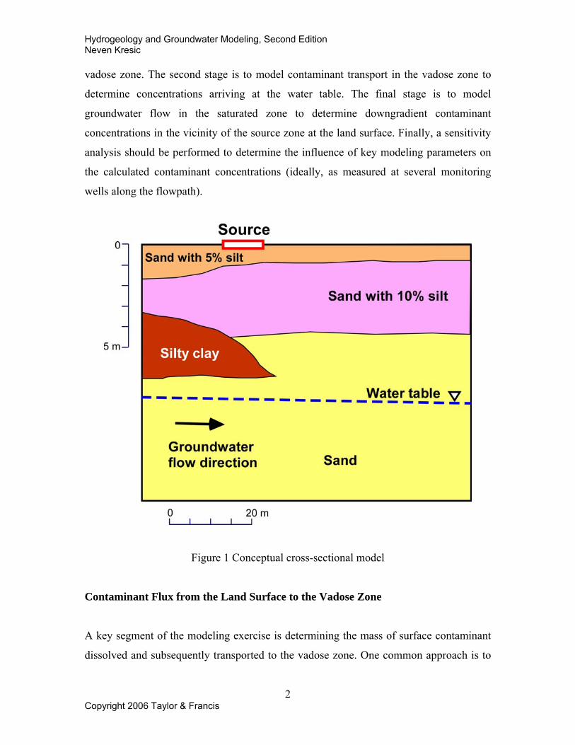
precipitation in the area is 49.4 inches. Figure 1 shows soil types underlying the site in

both the vadose and saturated zones, as well as the average position of the water table. No

information is available on possible vertical hydraulic gradients in the unconfined

aquifer, so the groundwater flow is assumed to be only in the horizontal direction. The

sorption of the contaminant onto soils is assumed to be linear, with the adsorption

(partitioning) coefficient estimated to be 0.07 L/kg for the surficial sand (5% silt), 3.5

L/kg for the silty clay, and 0.21 L/kg for both the sand with 10% silt and the aquifer sand.

The contaminant is known to be recalcitrant (not readily biodegradable). Based on the

available information, develop a cross-sectional (two-dimensional) numeric model for

both the vadose zone and the saturated zone below the source area. Use the model to

predict contaminant dissolved concentrations as it leaches from the land surface, for the

first 15 years of active contaminant loading, followed by additional 15 years after the

loading was discontinued.

Summary: The primary objective of the unsaturated-saturated groundwater model is to

demonstrate how the contaminant residing on the ground surface can leach to the

saturated zone through the vadose zone, and subsequently migrate in the saturated zone

off the immediate aquifer portion underlying the source area. Ideally, the model should

closely match contaminant concentrations observed in monitoring wells installed in the

source zone and downgradient from it. However, such information is not available in this

case. The model development is essentially a three-stage task. The first component is to

use contaminant loading data to determine the concentration of contaminant entering the



vadose zone. The second stage is to model contaminant transport in the vadose zone to

determine concentrations arriving at the water table. The final stage is to model

groundwater flow in the saturated zone to determine downgradient contaminant

concentrations in the vicinity of the source zone at the land surface. Finally, a sensitivity

analysis should be performed to determine the influence of key modeling parameters on

the calculated contaminant concentrations (ideally, as measured at several monitoring

wells along the flowpath).

Figure 1 Conceptual cross-sectional model

Contaminant Flux from the Land Surface to the Vadose Zone

A key segment of the modeling exercise is determining the mass of surface contaminant

dissolved and subsequently transported to the vadose zone. One common approach is to



use contaminant dissolution rate combined with an infiltration time of one year to

estimate this loading on the annual basis. In other words, it is assumed that the

contaminant dissolution facilitates calculation of contaminant concentrations at the

uppermost model boundary, i.e., model boundary condition at the land surface. This

boundary condition is applicable to the length of the source zone at the land surface, in

the direction of groundwater flow. For one square meter of soil, an infiltration volume

and contaminant mass loading can be calculated from site specific data. As long as this

mass loading is less than the maximum amount dissolvable in one year (calculated as the

product of the saturated concentration in water and the infiltration volume), it can be

assumed that 100 percent of the mass loading is dissolved through percolation. The

contaminant concentration entering the vadose zone is then expressed as the annual mass

loading per square meter divided by the annual infiltration volume per square meter.

As stated previously, annual average rainfall in the area is 49.4 inches. As surficial soils

are well drained (sand with 5% silt), 30 percent of this precipitation is assumed to

recharge groundwater, resulting in the infiltration rate of 14.82 in/yr. Converted to metric

units and spread over one square meter, this equates to 376 L/m2/yr.

The next step is determining whether this volume of water is sufficient to dissolve the

contaminant present at the surface. Based on the contaminant characteristics, more than

enough recharge is available to dissolve the contaminant mass loaded at the land surface

during the entire 15-year period. Therefore, the contaminant concentration in recharge

percolating through the source zone can be computed as the annual mass loading in kg/m2

divided by 376 L/m2/yr. The results of this calculation are given in Table 1.

Table 1 Peak Dissolution Rate Computation, Mass Loading Data, and Percolate Concentration

Infiltration (L/m2/yr)

Solubility (mg/L)

Peak Mass Dissolution (mg/m2/yr)

Mass Loading (mg/m2/yr)

Percolate Concentration (mg/L)

376 59.9 22,548 20.9 0.055



Modeling Flow in the Vadose Zone

The vadose zone is defined as the subsurface area where soil moisture content is below

its saturated value. Flow in the vadose zone can be best understood through interpretation

of Darcy’s Law for unsaturated flow in one dimension:

( ) ( )( )zhz

KKq rs −∂∂

−= θθ

where q is flow per unit width, Ks is the saturated hydraulic conductivity, Kr is the

relative hydraulic conductivity (or the ratio of unsaturated to saturated hydraulic

conductivity), θ is the soil moisture content, z is the elevation potential, and h is the

pressure head. The pressure and elevation heads combine to form the total hydraulic

head. Pressure head is negative in the unsaturated zone, zero at the water table, and

positive in the saturated zone. In the vadose zone, pressure head is also known as matric

head, and is a measure of the capillary pressure acting on a volume of fluid. In VS2DTI,

the datum for the elevation head is the ground surface, with the downward Z-direction

being positive.

Darcy’s Law illustrates the complexity of unsaturated flow, as both relative hydraulic

conductivity and pressure head are functions of the soil moisture content (θ). Due to this

difficulty, empirical relationships are necessary to model unsaturated conductivity and

calculate flow in the vadose zone. The empirical solution scheme used for the model is

that of van Genuchten (1980). Relative hydraulic conductivity and soil moisture content

are calculated as functions of the pressure head. The equations of van Genuchten relate

moisture content to pressure head through the effective saturation (Se) as:

[ ] NN

N

rs

re hS

−

+=−−

=1

||1 αθθθθ

where: α (1/length) and N are curve shape parameters, θr is the residual moisture content,

and θs is the saturated moisture content (Lappala et al, 1987). This equation is essentially

a curve fit to the soil moisture-characteristic curve, and can be integrated to yield the

relationship for effective hydraulic conductivity (Lappala et al, 1987):



NN

NN

r

D

CDK

21

21

1

−

−

⎟⎟⎠

⎞⎜⎜⎝

⎛−

=

where 1|| −= NhC α and NhD ||1 α+=

The curve fit parameters and pressure head can also be used to solve for the specific

moisture capacity, or the slope of the moisture-characteristic curve ⎟⎠⎞

⎜⎝⎛∂∂

tθ (Lappala et al,

1987). This equation is defined by van Genuchten (1980), and is written as follows:

( )( )

NN

N

r

h

hnN

t 1

1

1

1

−

−

⎥⎥⎦

⎤

⎢⎢⎣

⎡⎟⎠⎞

⎜⎝⎛+

⎟⎠⎞

⎜⎝⎛−−

=∂∂

αα

αθ

θ

where n is the total porosity (also equivalent to the saturated moisture content).

At the first time step, the initial pressure head can be used to calculate specific moisture

capacity and relative conductivity. These parameters can then be used to solve for total

head at the next time step by applying the two-dimensional form of Darcy’s Law and the

continuity equation in finite difference form.

Modeling Flow in the Saturated Zone

Flow in the saturated zone is easier to model as hydraulic conductivity and moisture

content are constant for a given soil textural class. Variations in conductivity arise due to

heterogeneities in aquifer formations, but this is accounted for through the dispersivity

parameter. Darcy’s Law in one dimension for saturated flow is:

( )zhz

Kq s +∂∂

=



Where h is the pressure head and z is the elevation head. Pressure head is always positive

in the saturated zone, and the datum for elevation head is mean sea level. Any elevation

above sea level is interpreted as being positive.

Model Selection

As described in the problem statement, a groundwater model is needed that can simulate

contaminant fate and transport in both the unsaturated (vadose) and saturated zones. The

United States Geological Survey (USGS) public domain program VS2DTI (see Lappala

et al., 1987; Healy, 1997; and Hsieh et al., 1999) version 1.3 was utilized for the

following reasons: 1) it solves the groundwater flow equation in both the vadose and

saturated zones simultaneously, and 2) it has a user-friendly graphic pre- and post-

processor in Microsoft Windows environment. The United States Department of

Agriculture (USDA) public-domain program Rosetta (see Schaap et al., 2001) version 1.2

was used to estimate van Genuchten curve fit parameters for the unsaturated flow

equations, saturated hydraulic conductivities, and total porosities for all soils at the range.

Rosetta is also user-friendly, and combines with VS2DTI to form a versatile

unsaturated/saturated modeling package that is publicly available for download from the

internet.

Model Domain & Grid

VS2DTI is a two-dimensional modeling program, and it is necessary to define a domain

spanning the X (length) and Z (depth) directions. For this problem the domain length in

the X-direction is 80 meters (approximately 262 feet). The source area has a roughly

square shape of 10 meters x 10 meters. The Z-direction domain is 12. 5 m. The model

grid is uniform and has 50 columns and 20 rows as shown in Figure 2.

Soil Textural Classes

The model domain in VS2DTI is divided into distinct soil regions, known as textural

classes, which can be represented by polygons drawn in the X and Z directions. These

soil types are then assigned values for the parameters governing water flow, and

contaminant fate and transport in the unsaturated and saturated zones. As the sand-silt-



clay percentages are estimated for each textural class, Rosetta version 1.2, Model 1 can

be used to predict van Genuchten parameters for flow in the vadose zone, including

saturated hydraulic conductivity. The percentages for each soil type are entered into the

Rosetta interface, and the results are displayed in an output database. Note that the

Rosetta-derived parameters for predominantly clayey and pure-clay soils are somewhat

less reliable compared with other soil types, primarily because the original experimental

data utilized for the underlying analysis in Rosetta had a small number of clayey soil

samples, non of which was pure clay. It is therefore advisable to make appropriate

corrections to the Rosetta-offered parameter values in case a model includes clays. For

example, the lowest available saturated hydraulic conductivity for “clay” in Rosetta is on

the order of 10-5 cm/sec, whereas practice shows that pure clays have saturated hydraulic

conductivity commonly 10-7 cm/sec or lower. Table 2 shows soil parameters for our case

based on the Rosetta results.

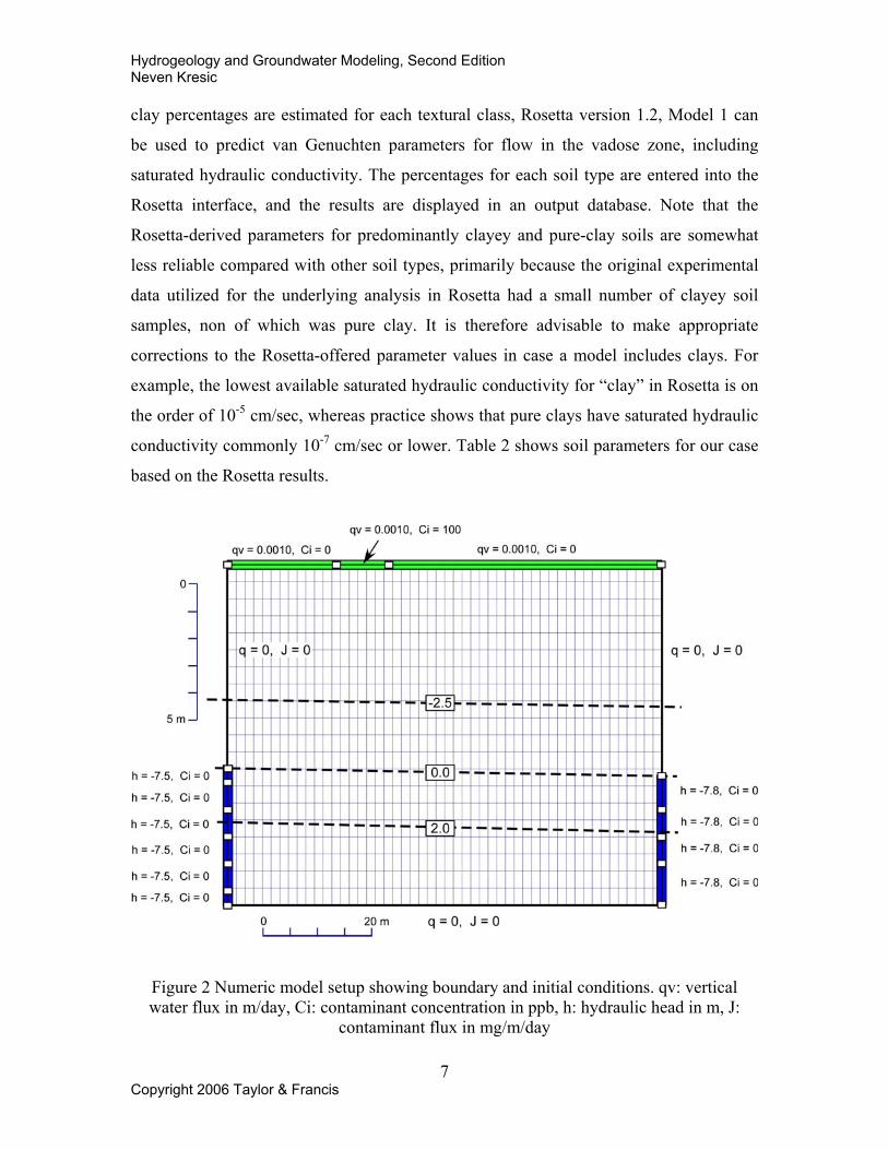
Figure 2 Numeric model setup showing boundary and initial conditions. qv: vertical water flux in m/day, Ci: contaminant concentration in ppb, h: hydraulic head in m, J:

contaminant flux in mg/m/day



The model also requires an estimate of the total porosity for each textural class. Total

porosity is assumed to be equivalent to the saturated water content as estimated by

Rosetta, since all available soil voids are filled with water upon saturation. A final

assumption required for each textural class is the ratio of vertical hydraulic conductivity

to horizontal hydraulic conductivity. In our case this ratio is assumed to be unity. In other

words, groundwater will flow vertically as easily as it will horizontally.

Table 2 Soil Parameters Estimated by Rosetta. Note that the saturated hydraulic conductivity for “silty clay” was adjusted.

Saturated

Hydraulic Conductivity

Residual Moisture Content

Saturated Moisture Content

Alpha N Porosity

Textural Class Ks (m/day) θr θs α (1/m) N (1/m) n

Sand 5% Silt 7.67 0.0460 0.384 3.83 3.54 0.384

Sand 10% Silt 3.77 0.0403 0.389 4.30 2.75 0.389

Aquifer Sand 7.67 0.0460 0.384 3.83 3.54 0.384

Silty Clay 0.035 0.0680 0.408 0.80 1.09 0.408

Fate and Transport Parameters

Sorption

An important parameter of the model is simulating how the contaminant adsorbs to soil

particles while moving through the subsurface environment. The two parameters

influencing contaminant adsorption are the soil bulk density (ρb), and the bulk solid/water

partitioning coefficient (Kd). Traditionally, the bulk density is expressed in kg/L, while

Kd is expressed in L/kg (assuming a linear sorption isotherm). As long as the product of

the bulk density and Kd is dimensionless, the numbers are suitable for input into the

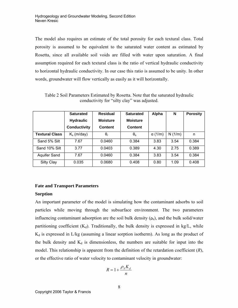
model. This relationship is apparent from the definition of the retardation coefficient (R),

or the effective ratio of water velocity to contaminant velocity in groundwater:

nK

R dbρ+= 1



The contaminant is known to exhibit retardation due to adsorption onto the soil matrix. In

the model, values for bulk density and Kd must be defined for each textural class. The

bulk density can be estimated by the equation:

( ) sb n ρρ −= 1

where n is the soil porosity as estimated by Rosetta, and ρb is the individual soil particle

density. The individual soil particle density is assumed to be that of silica (2.65 kg/L) for

all soil types in this study. The site-specific textural classes in our case have the following

bulk densities (in kg/L): 1.63 for surficial sand and aquifer sand, 1.57 for silty clay, and

1.62 for sand with 10% silt.

Definition of Kd values for each textural class has greater uncertainty. Kd is a function of

both the contaminant of interest and the soil through which the contaminant migrates. For

organic constituents, Kd is traditionally calculated as the product of the fraction of organic

carbon in the soil matrix (foc) and the organic-carbon partition coefficient of the

contaminant (Koc). In our case, Kd values were determined based on laboratory tests as

indicated in the statement of problem: 0.07 L/kg for the surficial sand (5% silt), 3.5 L/kg

for the silty clay, and 0.21 L/kg for both the sand with 10% silt and the aquifer sand.

Dispersion

In numeric groundwater modeling, dispersivity is traditionally a flexible parameter used

to calibrate the model and minimize computational errors. One of the goals in this

process is to reduce “numeric” dispersion, or errors caused by the finite difference

method that exaggerate dispersion effects. A key dimensionless parameter that dictates

field scale dispersivity is the Peclet number. The Peclet number illustrates the relative

importance of advective transport compared to dispersive transport, and can be calculated

as:

LDvLPe =

where v is the average seepage velocity, L is the length scale, and DL is the coefficient of

longitudinal dispersion (length2/time) (Chin, 2000). In finite difference modeling, the

length scale can be interpreted as the grid spacing in the longitudinal direction (which in



the case of VS2DTI signifies the X-direction). Taken with the assumption that advective

transport dominates over the model space, the Peclet number can be redefined as:

L

LPeα

=

where L is the longitudinal grid spacing, and αL is the longitudinal dispersivity (length

units). Longitudinal dispersivity is driven by macrodispersion, or significant variation in

hydraulic conductivity in the primary direction of flow (Chin, 2000). In general, the

Peclet number should be less than 2 to prevent numeric dispersion. However, it has also

been shown that many models can resist numeric dispersion with Peclet numbers as high

as 10. In our model, the longitudinal dispersivity is 0.5 m, which for the cell size of 1.6 m

in the X direction gives the Peclet number of approximately 3. Transverse dispersivity is

thought to be driven by time variations in seepage velocity, and is generally significantly

smaller than its longitudinal counterpart. Field studies have shown that the ratio of αL to

αT usually ranges from 6 to 20. While traditional practice is to select a ratio of 10, the

associated αT value seems to exaggerate transverse dispersion in our model. Under the

assumed boundary conditions, there should be no temporal variation in seepage velocity,

thus minimizing transverse dispersion. Therefore, the selected αL/αT ratio was increased

to 15, which gives the transverse dispersivity of 0.033 m.

Degradation (Transformation) Rate

Another key parameter for contaminant fate and transport modeling is the transformation,

or degradation, rate. In our case, however, because the contaminant is generally thought

to be recalcitrant (not readily biodegrade), the degradation rate is assumed to be zero

although there is no site-specific information to confirm this assumption.

Diffusion

VS2DTI fate and transport modeling also requires definition of the molecular diffusion

constant (length2/time). Molecular diffusion in water always occurs, even in the presence

of zero flux conditions, but is of a very small magnitude. Further reducing diffusion in

groundwater is the constrained, sinuous flow path a solute must take through porous

media. The ratio of actual flow path length to straight line distance is known as tortuosity.



Tortuosity values typically vary from 2 for coarse sands, to 100 for ultra fine clays (Chin,

2000). Combined with a measure of the effective porosity (ne), or the percentage of

interconnected pore space, the effective molecular diffusion coefficient (De) can be

determined through the relationship:

τwe

eDn

D =

where Dw is the molecular diffusion in water.

This analysis proves unnecessary in our case. Typical values for molecular diffusion of

major cations and anions in water range from 8.64x10-5 to 1.73x10-4 m2/day. When

considering the added reduction caused by tortuosity and effective porosity, this value

loses even more significance when compared to the grid spacing. Assuming a value on

the order of 10-5 m2/day would have minimal influence on the results. Furthermore,

estimates of effective porosity and tortuosity for the soils at our site are not available.

Therefore, an effective molecular diffusion constant of zero is assumed.

Specific Storage

In essence, the specific storage measures the elastic storage capacity of the soil matrix.

The model requires an estimation of the specific storage for each defined textural class.

Specific storage is quite small, with typical values at 0.0005 m-1 or less. In our case, for

simplification purposes, the 0.00033 m-1 value is used for each soil type, which is

anticipated to have little effect on the fate and transport of the contaminant. Theoretically,

the unsaturated areas of the model should have specific storage values of zero.

Unfortunately, VS2DTI must see a non-zero value to solve properly. Once again, this

inaccuracy is not anticipated to affect results as there is no groundwater pumping or

drawdown simulated in the model.

Initial Pressure Head & Concentration

VS2DTI requires definition of the initial pressure head and contaminant concentration

across the model domain. The initial pressure head is established with user-defined

contour lines that VS2DTI can interpolate between to define initial conditions across the



entire domain. For our model, three open contour lines are drawn that extend beyond the

domain to ensure accurate interpolation. The middle line is the zero pressure head

contour that traces the top of the water table. The two addition lines are drawn parallel to

the zero pressure line; one 2.5 meters above, and the other 2 meters below. These lines

are assigned pressure heads of 2.0 meters, and -2.5 meters respectively. The initial

contaminant concentration of the contaminant is assumed to be 0.0 ppb. This condition is

defined with a closed contour that surrounds the entire domain.

Alternatively, the initial equilibrium profile can be used to define the initial location of

the water table. This method is much simpler and does not involve interpolation. Upon

selection of this method, VS2DTI prompts the user to enter the Z-coordinate of the water

table, followed by the minimum allowable pressure head. As long as the minimum

pressure head is a negative value represented by a line above the datum, the model will

perform adequately. The only downside to this method is the inability to slope the water

table. However, as this only marks an initial condition, the model calculates the position

of the new water table based on boundary conditions at the first time step. Therefore the

beginning inaccuracy is insignificant in terms of model results.

Boundary Conditions

Essential to adequate representation of groundwater flow at the site are well-defined

boundary conditions. VS2DTI only allows boundary condition assignment between

vertices on the exterior of the model domain. The user must selectively place the

appropriate number of vertices to delineate constant head or constant flux boundaries

such as surface water bodies or confining layers. Boundary conditions are defined in the

model for every recharge period. A recharge period is simply a period of time with

constant boundary conditions. This simplifies the process of changing contaminant

loadings, recharge quantities, or groundwater gradients over time.

In our case, the boundary conditions are assigned over two recharge periods based on the

constant loading over the 15-year period, followed by another 15 years of no loading. The

source zone and the rest of the land surface (i.e. the Z = 0 domain boundary) receives a



constant vertical flux of water into the domain for both recharge periods. The flux

quantity is equal to 0.001 m/day, which is the assumed infiltration rate of 14.82 in/yr

converted to metric units. The influent contaminant concentration is zero for all areas

along the Z = 0 boundary except the source zone, where the concentration is set to the

one calculated in Table 1. The second recharge period begins after first 15 years, when

the contaminant loading at the land surface was discontinued.

Constant total head boundary conditions are assigned along the left-hand and right-hand

vertical limits of the domain to reflect the average horizontal hydraulic gradient in the

aquifer beneath the source zone. The model defines total head in terms of the vertical

distance from the Z = 0 line. The user manual suggests thinking of the total head at a

point as the elevation to which water would rise in a piezometer opened to that point.

As no vertical gradients have been measured at the site, the left-hand side of the domain

boundary below the water table elevation is assigned a constant total head of -7.5 meters.

The area between the land surface and the water table is given a possible seep boundary

condition, as there is no barrier to groundwater flow, nor a hydraulic head to define. The

model determines whether a seep condition should develop along the boundary upon

initiation. If seepage occurs, the pressure head is set to zero and flow can exit the

boundary. If not, the boundary becomes a zero flux condition. The right-hand side of the

domain boundary is set up in an identical fashion. A constant total head is established

from the water table to the bottom of the domain. The right-hand side total head is -7.8

meters, as calculated from the measured average horizontal hydraulic gradient of

0.00375. The segment between the water table and the land surface is once again a

possible seepage face, leaving room for the water table to rise if so determined by the

model.

The bottom of the model is simulated with a zero flux boundary condition. Without

vertical gradients, the plume is not expected to approach the bottom of the model domain

in the general site area. If the plume approached the bottom of the domain, constant head

boundaries would be necessary to allow flow to pass through the bottom. Otherwise, the



solute would accumulate at the bottom boundary and interfere with model results. Figure

2 shows the boundary conditions as entered into the VS2DTI model domain, as well as

the distribution of initial pressure head. Note that the initial contaminant concentration in

the water flux (percolation) entering the vadose zone in the source area is shown as 0.1

mg/L instead of 0.055 mg/L calculated in Table 1. This higher value was used in one the

model sensitivity runs.

Simulation Settings

An important model parameter is the time step determination. Excessively long time

steps can hinder accuracy and cause numeric dispersion. Similar to the Peclet number’s

analysis of grid spacing, the Courant number measures the appropriateness of the time

step settings for the model. The Courant number can be defined as the distance water

travels in the X- or Z-direction during a time step divided by the grid spacing in that

particular dimension, or:

LtvCr

Δ=

where v is the X- or Z-direction groundwater velocity, Δt is the time step, and L is the

grid length in the direction of interest. Common practice dictates that the maximum

possible Courant number in a grid should be less than or equal to unity to ensure accurate

numeric convergence. In our model, the highest velocity to grid dimension ratio occurs

near the bottom of the model, where X-direction velocities are the highest. The X-

direction grid spacing is 1.6 m, and the maximum X-direction velocity is 0.1 m/day based

on preliminary runs of the model. Therefore, any time step less than 16 days is adequate

to keep the Courant number less than 1. As a result, the maximum time step allowable in

the model is set to 16 days.

Other simulation settings include selection of the units, solver method, and solution

closure criterion. Model units are chosen to minimize conversions from Rosetta output

and the contaminant loading data. Mass is expressed in milligrams, length in meters, and

time in days. This is adequate for the solute fate and transport modeling as the displayed

concentration is in mg/m3, equal to μg/L or parts-per-billion (ppb). The difference



scheme is selected to be centered in space and time, which yields the most accurate

result. However, oscillations are more prevalent in centered difference schemes,

increasing the importance of Peclet and Courant number monitoring. The arithmetic

mean is used to interpolate varying hydraulic conductivities, the preferred method for

VS2DTI. The minimum number of iterations per time step is set to 2, and the maximum

to 1000. Closure criterion for head is set to 0.0001 m to minimize flow errors. Closure

criterion for solute is 0.1 ppb to reduce computational effort. Slightly greater error will

occur for the solute balance, but the uncertainty of the contaminant loading estimates

makes this error insignificant.

Another model assumption is a steady state criterion of 0.0 ppb. This essentially means

steady state can never be assumed during a recharge period, and the model must solve

finite difference equations at every time step. In addition, a ponding height of 0.0 m is

assumed, meaning that water does not build up on top of the model domain (i.e. the land

surface for the model). Ponding would normally occur if the recharge rate exceeded the

seepage capacity of the surface soils. This is not anticipated to happen as the total annual

recharge quantity is divided into a smaller daily rate. In other words, recharge is modeled

as a year long precipitation with low intensity. Finally, no evaporation or

evapotranspiration is modeled. Evaporation is ignored to maintain model simplicity, and

evapotranspiration is assumed insignificant due to the barren landscape of the site.

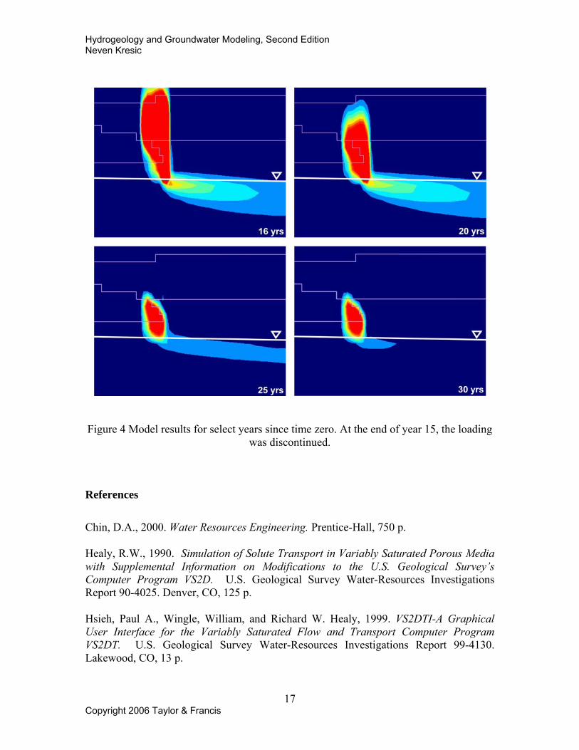
Results and Discussion

Figure 3 and Figure 4 show results of the model simulation for different time intervals

since the start of contaminant loading at the land surface. The loading was discontinued

at the end of year 15, so that the result for year 16 shows the effect of flushing by the

newly percolating water with 0 concentration. Arguably the most interesting result is the

effect of clay on contaminant fate and transport. Due to low hydraulic conductivity and

contaminant sorption, the clay lens acts as a long-term storage, and a secondary source of

dissolved contaminant in the saturated zone. The model results are also compiled as

animation, showing advancement and the subsequent retreat of the contaminant plume.



Figure 3 Model setup (top left) and model results for select years since time zero (the beginning of contaminant loading at the surface).



Figure 4 Model results for select years since time zero. At the end of year 15, the loading was discontinued.

References

Chin, D.A., 2000. Water Resources Engineering. Prentice-Hall, 750 p. Healy, R.W., 1990. Simulation of Solute Transport in Variably Saturated Porous Media with Supplemental Information on Modifications to the U.S. Geological Survey’s Computer Program VS2D. U.S. Geological Survey Water-Resources Investigations Report 90-4025. Denver, CO, 125 p. Hsieh, Paul A., Wingle, William, and Richard W. Healy, 1999. VS2DTI-A Graphical User Interface for the Variably Saturated Flow and Transport Computer Program VS2DT. U.S. Geological Survey Water-Resources Investigations Report 99-4130. Lakewood, CO, 13 p.



Lappala, E.G., Healy, R.W., and E.P. Weeks, 1987. Documentation of Computer Program VS2D to Solve the Equations of Fluid Flow in Variably Saturated Porous Media. U.S. Geological Survey Water-Resources Investigations Report 83-4099. Denver, CO, 184 p. Schaap, M.G., Leij, F.J., and M.T. van Genuchten, 2001. ROSETTA: a computer program for estimating soil hydraulic parameters with hierarchical pedotransfer functions. Journal of Hydrology 251 (2001) 163-176. Van Genuchten, M.Th., 1980. A closed-form equation for predicting the hydraulic conductivity of unsaturated soils. Soil Sci. Am. J., 44:892-898.

modeling of leachate concentration in unsaturated and ... · hydrogeology and groundwater modeling,...

Documents