modeling of hybrid marine electric propulsion systems

Modeling of Hybrid Marine Electric Propulsion Systems

Øyvind Rønneberg Gåsemyr

Marine Technology

Supervisor: Eilif Pedersen, IMT

Department of Marine Technology

Submission date: June 2014

Norwegian University of Science and Technology

Preface

The M.Sc. thesis is mandatory for all master students attending the Departmentof Marine Technology at NTNU in Trondheim. The thesis accounts for 100 % ofthe workload during the tenth semester and is equal to 30 ECTS.

The subject of the thesis was developed in collaboration with the Departmentof Marine Technology at NTNU in Trondheim and ABB Marine. The subject wasadjusted to meet my background and interest as far as possible.

The thesis revolves around modeling and simulation of diesel-electric power sys-tems utilizing energy storage devices in order to reduce load variations on the powerplant, hence reducing emissions and increasing fuel efficiency.

I would like to thank Associate Professor at NTNU, Eilif Pedersen for guidanceand assistance during the thesis work. I would also like to thank Børre Gundersen(R&D manager at ABB) and Kristoffer Dønnestad (R&D engineer at ABB) forproviding technical assistance throughout the project.

Øyvind Rønneberg Gasemyr, Trondheim 10.06.2014

I

Abstract

Energy storage devices integrated in diesel-electric power systems is believed tohave potential also in marine applications. For certain load conditions energy stor-age can act as load buffers which will decrease the load variations on the generatorsets, hence optimizing the operation when is comes to emissions and fuel efficiency.

In this context this thesis is aimed at development of simulation tools for hybridmarine electric propulsion systems. Assessment of two energy storage concepts isincluded, focusing on how their different attributes is utilized in the best manner.The bond graph language is chosen for modeling the physical components, becauseof its ability to represent the power interaction between a large selection of energydomains.

Component models of the essential electrical and mechanical components on theconsumer side of a conventional diesel-electric propulsion system is modeled andconnected. Additionally component models of a rechargeable battery and a super-capacitor is implemented to the model. A simple power control method is used tocontrol the power flow of the energy storage devices .

Hybrid power plants are complex systems and the simulation tool developed inthis thesis is considered far from complete, especially when it comes to controlsystems. To determine the actual reduction in fuel efficiency and emissions, dy-namic models of diesel engines and generators should be added. However the modelserves as a promising basis for further development. It visualizes the peak shavingeffect from the power input point of view as expected and the principles of utilizingenergy storage under varying load conditions.

II

Contents

Preface I

Abstract II

Table of Contents IX

List of Tables IX

List of Figures X

Nomenclature X

1 Introduction 11.1 Motivation . . . . . . . . . . . . . . . . . . . . . . . . . . . . . . . . 11.2 Problem . . . . . . . . . . . . . . . . . . . . . . . . . . . . . . . . . . 1

1.2.1 Scope of work . . . . . . . . . . . . . . . . . . . . . . . . . . . 21.3 Organization of the thesis . . . . . . . . . . . . . . . . . . . . . . . . 2

2 Diesel-electric propulsion systems 32.1 Conventional system description . . . . . . . . . . . . . . . . . . . . 42.2 Drivers for change . . . . . . . . . . . . . . . . . . . . . . . . . . . . 52.3 New technologies and future aspects . . . . . . . . . . . . . . . . . . 6

2.3.1 Fuels cells in marine applications . . . . . . . . . . . . . . . . 62.3.2 Propulsion systems using pure battery power . . . . . . . . . 72.3.3 Hybrid system development . . . . . . . . . . . . . . . . . . . 72.3.4 The onboard DC Grid . . . . . . . . . . . . . . . . . . . . . . 7

3 Energy storage devices 113.1 Electrochemical batteries . . . . . . . . . . . . . . . . . . . . . . . . 12

3.1.1 Cell behavior during charging and discharging . . . . . . . . . 123.1.2 Battery Terminology . . . . . . . . . . . . . . . . . . . . . . . 133.1.3 Comparing different types of batteries . . . . . . . . . . . . . 153.1.4 Batteries and cells . . . . . . . . . . . . . . . . . . . . . . . . 16

3.2 Supercapacitors . . . . . . . . . . . . . . . . . . . . . . . . . . . . . . 163.2.1 Main types of supercapacitors . . . . . . . . . . . . . . . . . . 16

IV

3.2.2 Electric double-layer Capacitors . . . . . . . . . . . . . . . . 163.2.3 Requirements for achieving higher performance . . . . . . . . 173.2.4 Performance characteristics . . . . . . . . . . . . . . . . . . . 17

4 System Modeling 194.1 Bond graph modeling . . . . . . . . . . . . . . . . . . . . . . . . . . 194.2 Modeling of energy storage devices . . . . . . . . . . . . . . . . . . . 21

4.2.1 The Lithium ion battery . . . . . . . . . . . . . . . . . . . . . 214.2.2 Bond graph representation of the rechargeable battery . . . . 234.2.3 Building a battery pack . . . . . . . . . . . . . . . . . . . . . 24

4.3 The supercapacitor . . . . . . . . . . . . . . . . . . . . . . . . . . . . 254.3.1 Parameter determination . . . . . . . . . . . . . . . . . . . . 254.3.2 Bond graph representation of the supercapacitor . . . . . . . 28

4.4 The three-phase inverter . . . . . . . . . . . . . . . . . . . . . . . . . 294.4.1 Switched Power Junctions . . . . . . . . . . . . . . . . . . . . 304.4.2 Bond Graph representation of the 3-phase inverter . . . . . . 31

4.5 The induction motor . . . . . . . . . . . . . . . . . . . . . . . . . . . 324.5.1 Operating principle . . . . . . . . . . . . . . . . . . . . . . . . 324.5.2 Power invariant transformation . . . . . . . . . . . . . . . . . 334.5.3 Mathematical description of the power invariant transformation 334.5.4 Bond graph representation of the dq-transformation . . . . . 344.5.5 Mathematical model of the induction motor . . . . . . . . . . 364.5.6 Bond graph representation of the induction motor . . . . . . 38

4.6 Direct Torque Control . . . . . . . . . . . . . . . . . . . . . . . . . . 394.7 DC-DC Converter . . . . . . . . . . . . . . . . . . . . . . . . . . . . 434.8 The propeller . . . . . . . . . . . . . . . . . . . . . . . . . . . . . . . 434.9 Power flow control . . . . . . . . . . . . . . . . . . . . . . . . . . . . 44

4.9.1 SOC and voltage limitations . . . . . . . . . . . . . . . . . . 454.10 The complete power plant . . . . . . . . . . . . . . . . . . . . . . . . 46

5 Results 475.1 Simulation energy storage performance . . . . . . . . . . . . . . . . . 47

5.1.1 The battery pack . . . . . . . . . . . . . . . . . . . . . . . . . 475.1.2 Supercapacitor . . . . . . . . . . . . . . . . . . . . . . . . . . 485.1.3 Discussion . . . . . . . . . . . . . . . . . . . . . . . . . . . . . 49

5.2 Case simulations . . . . . . . . . . . . . . . . . . . . . . . . . . . . . 505.2.1 Case 1 - DP-operation with supercapacitor . . . . . . . . . . 505.2.2 Comments to case 1 . . . . . . . . . . . . . . . . . . . . . . . 525.2.3 Case 2 - Operation with a battery pack . . . . . . . . . . . . 525.2.4 Comments to case 2 . . . . . . . . . . . . . . . . . . . . . . . 54

6 Conclusions and recommendations 556.1 Recommendations for further work . . . . . . . . . . . . . . . . . . . 56

References 57

V

Appendices i

A Parameter Calculation for the Induction motor iiA.1 No-load test . . . . . . . . . . . . . . . . . . . . . . . . . . . . . . . . iiA.2 Blocked rotor test . . . . . . . . . . . . . . . . . . . . . . . . . . . . vA.3 Calculation of inductance parameters and rotational losses . . . . . . viiA.4 Test report of the induction motor . . . . . . . . . . . . . . . . . . . ix

B Source code from 20-Sim xB.1 Mse, battery . . . . . . . . . . . . . . . . . . . . . . . . . . . . . . . xB.2 SOC-Calculator . . . . . . . . . . . . . . . . . . . . . . . . . . . . . . xB.3 Torque and flux determination . . . . . . . . . . . . . . . . . . . . . xiB.4 Switching table . . . . . . . . . . . . . . . . . . . . . . . . . . . . . . xiiB.5 Sector determination . . . . . . . . . . . . . . . . . . . . . . . . . . . xvB.6 1s-junction . . . . . . . . . . . . . . . . . . . . . . . . . . . . . . . . xvB.7 0s-junction . . . . . . . . . . . . . . . . . . . . . . . . . . . . . . . . xviB.8 Rotor and propeller inertia . . . . . . . . . . . . . . . . . . . . . . . xviB.9 Propeller load . . . . . . . . . . . . . . . . . . . . . . . . . . . . . . . xviB.10 TF, induction motor . . . . . . . . . . . . . . . . . . . . . . . . . . . xviiB.11 I, rotor and stator current . . . . . . . . . . . . . . . . . . . . . . . . xviiB.12 Rotational losses . . . . . . . . . . . . . . . . . . . . . . . . . . . . . xviii

VI

List of Tables

4.1 Basic bond graph elements and their constitutive relations [20]. . . . 204.2 Sector determination table [22] . . . . . . . . . . . . . . . . . . . . . 424.3 Predefined switching table [22] . . . . . . . . . . . . . . . . . . . . . 42

5.1 Model parameters for the battery model . . . . . . . . . . . . . . . . 475.2 Model parameters for the supercapacitor . . . . . . . . . . . . . . . . 485.3 Reference torque . . . . . . . . . . . . . . . . . . . . . . . . . . . . . 52

A.1 Data for the induction motor, Type: M3BP 315MLA 4 IMB35/IM2001. . . . . . . . . . . . . . . . . . . . . . . . . . . . . . . . . . . . . . . ii

A.2 Results from No-load test . . . . . . . . . . . . . . . . . . . . . . . . iiiA.3 Results from blocked rotor test . . . . . . . . . . . . . . . . . . . . . vA.4 The parameters of the equivalent per-phase circuit for the induction

motor . . . . . . . . . . . . . . . . . . . . . . . . . . . . . . . . . . . vi

VII

List of Figures

2.1 Conventional electric power and propulsion plant for a typical off-shore support vessel [2]. . . . . . . . . . . . . . . . . . . . . . . . . . 4

2.2 MARPOL Annex VI, (NOx) emission limits [3]. . . . . . . . . . . . . 52.3 Basic principle of a fuel cell [5]. . . . . . . . . . . . . . . . . . . . . . 62.4 Typical fuel efficiency curve for diesel engines operating at constant

speed [1]. . . . . . . . . . . . . . . . . . . . . . . . . . . . . . . . . . 82.5 Single line diagram for a diesel-electric propulsion system with the

Onboard DC grid installed[6]. . . . . . . . . . . . . . . . . . . . . . . 92.6 Fuel efficiency plot for diesel engines operating at variable speed [6]. 9

3.1 Ragone plot of different types of energy storage devices [10]. . . . . . 113.2 Essential components of a basic electrochemical cell [5]. . . . . . . . 133.3 Discharge and charge curves of a 1.25 V cell [12]. . . . . . . . . . . . 143.4 Ragone diagram for various electrochemical batteries [12] . . . . . . 153.5 structure of electric double-layer capacitors [13]. . . . . . . . . . . . . 17

4.1 Power bond . . . . . . . . . . . . . . . . . . . . . . . . . . . . . . . . 194.2 Discharge characteristics of a rechargeable battery [14]. . . . . . . . 224.3 Mathematical battery model. . . . . . . . . . . . . . . . . . . . . . . 234.4 Bond graph representation of battery . . . . . . . . . . . . . . . . . 234.5 Bond graph representation of a battery pack. . . . . . . . . . . . . . 244.6 Basic conceptual model of a supercapacitor [18] . . . . . . . . . . . . 254.7 Typical voltage profile for charging and discharging of a supercapac-

itor [19] . . . . . . . . . . . . . . . . . . . . . . . . . . . . . . . . . . 264.8 Non-simplified bond graph representation of the conceptual super-

capacitor model. . . . . . . . . . . . . . . . . . . . . . . . . . . . . . 284.9 Simplified bond graph representation of the conceptual supercapac-

itor circuit. . . . . . . . . . . . . . . . . . . . . . . . . . . . . . . . . 294.10 3-phase transistor inverter [24]. . . . . . . . . . . . . . . . . . . . . . 294.11 Generalized 0s- and 1s-junctions [24] . . . . . . . . . . . . . . . . . . 304.12 Bond graph representation of the inverter . . . . . . . . . . . . . . . 314.13 Crossection of the induction motor (left) and the squirrel cage (right)

[25]. . . . . . . . . . . . . . . . . . . . . . . . . . . . . . . . . . . . . 324.14 Projection of the abc-frame on the direct, quadrate and stationary

axis [26]. . . . . . . . . . . . . . . . . . . . . . . . . . . . . . . . . . . 33

VIII

4.15 Bond graph representation if the Park’s transformation from theabc-frame to the dq-frame. . . . . . . . . . . . . . . . . . . . . . . . . 35

4.16 Bond graph model of the induction motor in the dq-frame lettingthe reference frame rotate with angular velocity, ωr. . . . . . . . . . 38

4.17 Control scheme using DTC for induction motor control . . . . . . . . 394.18 Voltage vectors [23] . . . . . . . . . . . . . . . . . . . . . . . . . . . . 414.19 Charging and discharging during load variations. . . . . . . . . . . . 444.20 Complete system model. . . . . . . . . . . . . . . . . . . . . . . . . . 46

5.1 Discharge curve of the battery, Ib = −100[A]. . . . . . . . . . . . . . 485.2 Simulation result of a complete charge-discharge cycle of the super-

capacitor. . . . . . . . . . . . . . . . . . . . . . . . . . . . . . . . . . 495.3 Load sharing, supercapacitor voltage and charging current. . . . . . 515.4 Propeller speed and electromagnetic torque . . . . . . . . . . . . . . 515.5 Load sharing, SOC and charging current from case simulation 2. . . 535.6 Propeller speed and electromechanical torque. . . . . . . . . . . . . . 53

A.1 Equivalent per-phase circuit for an induction motor . . . . . . . . . . iiiA.2 Equivalent per-phase circuit of the induction motor during No-load

test . . . . . . . . . . . . . . . . . . . . . . . . . . . . . . . . . . . . . iiiA.3 Equivalent per-phase circuit of the induction motor during the blocked

rotor test. . . . . . . . . . . . . . . . . . . . . . . . . . . . . . . . . . v

IX

NomenclatureAbbrevations

AC Alternating currentDC Direct currentDP Dynamic Positioning

DOD Depth of dischargeEB Electrochemical battery

ECA Emission Control AreaEDLC Electric double-layer capacitorEPR Equivalent parallel resistanceMCR Maximum continuous ratingOSV Offshore supply vesselPMS Power Management SystemPSV Platform Supply VesselSC Supercapacitor

SOC State of chargeSPJ Switched power junctionVSI Voltage Source Inverter

X

Uppercase

0 [-] Bond graph 0-junction1 [-] Bond graph 1-junctionA [V] Amplitude of exponential zoneA1, A2, A3 [-] Sector decision variableB [Ah1] Inverse of exponential zone time constantC [-] Bond graph capacitor elementCs [F] Equivalent capacitanceE0 [V] Constant Battery VoltageEc [J] Energy capacity of a capacitor bankGY [-] Bond graph gyratorI [-] Bond graph inertia ElementIb [A] Battery currentK [V] Polarization constantLs [H] Stator self-inductanceLr [H] Rotor self-inductanceLm [H] Mutual inductanceQ [Ah] Battery CapacityR [-] Bond graph resistor elementRi [Ohm] Internal ResistanceS1, S2, S3 [-] Inverter control variableSe [-] Bond graph effort sourceSf [-] Bond graph flow sourceTF [-] Bond graph transformerTp [Nm] Propeller load torqueVs [v] Equivalent voltageVT [V] Terminal Battery Voltage

XI

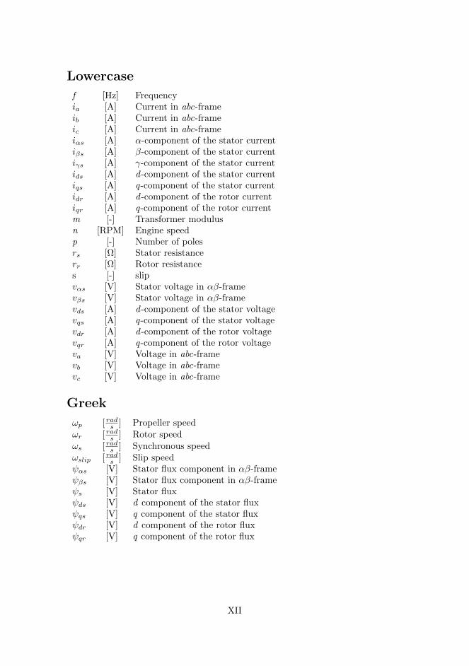
Lowercase

f [Hz] Frequencyia [A] Current in abc-frameib [A] Current in abc-frameic [A] Current in abc-frameiαs [A] α-component of the stator currentiβs [A] β-component of the stator currentiγs [A] γ-component of the stator currentids [A] d -component of the stator currentiqs [A] q-component of the stator currentidr [A] d -component of the rotor currentiqr [A] q-component of the rotor currentm [-] Transformer modulusn [RPM] Engine speedp [-] Number of polesrs [Ω] Stator resistancerr [Ω] Rotor resistances [-] slipvαs [V] Stator voltage in αβ-framevβs [V] Stator voltage in αβ-framevds [A] d -component of the stator voltagevqs [A] q-component of the stator voltagevdr [A] d -component of the rotor voltagevqr [A] q-component of the rotor voltageva [V] Voltage in abc-framevb [V] Voltage in abc-framevc [V] Voltage in abc-frame

Greek

ωp [ rads ] Propeller speedωr [ rads ] Rotor speedωs [ rads ] Synchronous speedωslip [ rads ] Slip speedψαs [V] Stator flux component in αβ-frameψβs [V] Stator flux component in αβ-frameψs [V] Stator fluxψds [V] d component of the stator fluxψqs [V] q component of the stator fluxψdr [V] d component of the rotor fluxψqr [V] q component of the rotor flux

XII

Chapter 1

Introduction

1.1 Motivation

Transient operation of diesel engines, caused by quick load variations is a significantsource for pollutant emissions. The effects of transient operation of diesel engines inmarine applications have gained more attention in recent years. There is believed tobe great benefits in analysis, modeling and simulations of both internal combustionengines and complete power systems. New solutions for control, optimization andsimulation are needed for the emerging hybrid marine power plants.

1.2 Problem

The focus in this thesis has been on development of a simulation model of a hybridmarine electrical power system using the bond graph method. Hybrid systems uti-lizes energy storage to optimize the operation when is comes to fuel consumptionand emissions. Component models of such energy storage devices is developed andimplemented. For this thesis a supercapacitor and a rechargeable battery is chosenfor energy storage. Modeling of hybrid power plants requires insight into severalenergy domains and engineering disciplines. Chemical energy trapped in the fuelis converted to thermal energy during combustion. Expansion of the trapped gasescreate a force on the piston, which generates mechanical torque on the engineshaft. Power is transformed from the mechanical domain to the electrical by con-necting the engine shaft to a generator. And by use of advanced control systemsand complex electrical components the desired propeller speed and torque is ob-tained. Flexible and accurate simulation models of multi-domain power plants areextremely useful and cost-effective compared to physical prototypes. On the otherhand modeling of these multi-disciplinary systems requires a large amount of effortand knowledge.

To limit the workload in this thesis to an acceptable level, the simulation model islimited to consist of the components on the consumer side of the power plant, in

1

1.3 Organization of the thesis

addition to the two energy storage devices. A simplified control unit for controllingthe power flow of the energy storage devices is also developed and added to themodel.

Both modeling and simulation has been carried out in the simulation and mod-eling software 20-sim.

1.2.1 Scope of work

• Investigate the emerging technologies in marine electric power systems andidentify the main differences and advantages compared to conventional ma-rine power systems.

• Identify the main benefits of energy storage devises in marine power systems.

• Perform a literature study on the concepts of energy storage and conversion,and the characteristics and principles of rechargeable batteries and superca-pacitors.

• Development of energy storage models.

• Development of models of the components on the consumer side of a hybridmarine electrical power system.

• Carry out performance simulations of the battery and the supercapacitor andrunning two case simulations of the complete model.

1.3 Organization of the thesis

Chapter 2: Includes a brief introduction to conventional diesel-electric propul-sion systems. New concepts and technologies which are applied and underdevelopment are also investigated.

Chapter 3: Presents a review of the main devices for energy storage and conver-sion, with emphasis on electrochemical batteries and supercapacitors.

Chapter 4: Presents the theoretical basis of the system components, along witha their bond graph representation. A brief introduction to the bond graphmethod is also included.

Chapter 5: Presents the simulation results of the two energy storage models andresults from two case simulations.

Chapter 6: Conclusion and recommendations for further work.

Appendix A: Presents the parameter calculations of the induction motor.

Appendix B: Source code from 20-sim for various model elements and compo-nents.

2

Chapter 2

Diesel-electric propulsionsystems

The use of electric propulsion is not a new idea, and the concept dates back to the1920s when steam generators were used in transatlantic passenger lines. But themore efficient and economical diesel engine eventually replaced the steam generatorin most applications. It was first when the AC motor drives was introduced in the1980s the use of electrical propulsion emerged in new applications [1]. Today diesel-electric propulsion systems can be found in cruise ships, field support vessels, semi-submersible drilling rigs, etc. The introduction of azimuth thrusters and poddedpropulsion units during the 1990s highlighted various advantages of diesel-electricpropulsion systems. [1] Summarizes the advantages of diesel-electric propulsion tothe following:

• Electric power can be fed through cables to electric motors at any location inthe vessel independent of the location of the prime mover. Thus increasingthe maneuverability and the space utilization of the vessel.

• The prime movers are usually represented by medium speed diesel engines,which have a lower weight and lower investment costs than equally rated lowspeed engines used in direct mechanical propulsion.

• Noise and vibration levels are reduced as a result of prime movers running atconstant speed, in addition to shorter shaft lines.

• The possibility to optimize the number of running generator sets to meetpower demands at different operational profiles (dynamic positioning, ma-neuvering, transit, etc.), thus reducing fuel consumption and air emissions.

• Reduced maintenance, as a result of optimal operation of the prime movers.

• The possibility to separate the propulsion systems physically to increase re-liability and to meet redundancy requirements.

3

2.1 Conventional system description

• Electric propulsion systems can provide maximum torque also at low speeds,which is important for ice going vessels where the propeller can be jammedor blocked with ice.

2.1 Conventional system description

Figure 2.1: Conventional electric power and propulsion plant for a typical offshoresupport vessel [2].

Today a conventional diesel-electric propulsion systems consists of multiple primemovers (diesel engines, gas engines, steam turbines, etc.), which acts as the sourceof power. The generators produce AC current with a frequency proportional to therotational speed of the prime mover. The AC current is distributed through themain switchboards to the different consumers on board the vessel. Transformersisolate the electric power distribution into several partitions with different voltagelevels to meet the requirements of the consumers (thrusters, hotel loads, auxiliaries,etc.). For vessels with dynamic positioning (DP) systems, the switchboard is splitin two, three or even four systems to meet redundancy requirements. The positionkeeping ability is then maintained, also upon worst case single failure of one section[1]. Electrical motors transform the electric power into mechanical power, whichis to be used for propulsion, cranes, winches, pumps, etc. Today most propulsionunits operate with fixed pitch, this means that the thrust only varies with thespeed of the propeller. The propeller speed is controlled through variable speeddrives which converts the frequency of the AC-current before it is supplied to theelectric motor. The voltage source inverter (VSI) is by far the most used converter.The switching elements of the rectifier and inverter in the VSI are controlled togive the electric motor the desired speed [1]. The overall control of the power

4

Chapter 2. Diesel-electric propulsion systems

system is performed by the power management system (PMS). The objective ofthe PMS is to ensure sufficient amount of available power for the actual operationmode. This is done by comparing the available power and the consumed power,and if needed, additional generators are started or stopped. By controlling andmonitoring the energy flow, the power management system utilizes installed andrunning equipment to ensure optimal fuel efficiency [1].

2.2 Drivers for change

During the 1990s the increased attention to the effect air pollution had on globalwarming led to new regulations restricting the content of nitrogen oxides (NOx),sulphur oxides (SOx) and particulate matter (PM) in the exhaust gas from dieselengines. MARPOL Annex VI sets limits for NOx emissions from diesel engines.The Tier levels refer to the maximum allowed NOx emissions per kWh produced.Tier I applies for all engine installed after January 2000. Tier II takes effect on allengines installed after January 2011, and calls for a NOx reduction of 16 - 22 %depending on the size of the engine. The Tier III standard will take effect as ofJanuary 2016, and calls for a reduction in NOx emission of 80 % relative to TierI, but its area of application restricted to Emission Control Areas (ECA). Areaswhich most likely will fall into this category are among others the North Seas, TheBaltic Sea and North America [3].

Figure 2.2: MARPOL Annex VI, (NOx) emission limits [3].

The legislation is stringent and national penalties for non-compliance can be severe.

5

2.3 New technologies and future aspects


2.3.1 Fuels cells in marine applications

Fuel cell technology has recently proved to be successful in marine applications,as demonstrated by the Fellowship project. The joint industry project resulted inthe installation of a 330 kW fuel cell in the offshore supply vessel Viking Lady,and has as of 2012 resulted for more than 7000 hours of smooth operation. Fuelcell technology builds on conversion of the chemical energy trapped in the fuelinto electrical energy through electrochemical reactions. The process itself is quitesimilar to the process in electrochemical batteries, where reactions occur at theinterface between the anode and cathode, though a continuous supply of air andfuel is required. Bi-products of the power generation from fuel cells are heat andH2O. The main advantages of introducing fuels cells to marine applications arean increased chemical efficiency, reduced CO2 emissions and reduced noise andvibration levels on board the vessel [4].

Figure 2.3: Basic principle of a fuel cell [5].

6


2.3.2 Propulsion systems using pure battery power

Lately there has been tremendous development in the energy storage technology,which enables vessels traveling short distances to utilize batteries as the only powersource. An example is the ferry designed and built by Siemens in cooperationwith Fjellstrand shipyard. The ferry which is operated by Norled AS runs onelectric power supplied by rechargeable lithium-ion batteries alone. The batteriesare recharged in 10 minutes each time the ferry docks to drop cars on and off, andare sized for crossing the fjords of western Norway. The ferry is designed optimallyin terms of weight and hull shape, to reduce the energy consumption. The ferrywhich has a capacity of 120 cars and 360 passengers is granted to serve the routebetween Lavik and Opedal from 2015 to 2025. The ferry currently serving thisroute consumes 1 million liters of diesel each year, and emits 2680 metric tons ofCO2 and 37 tons of NOx [6]. This enlightens the reduction of the environmentalfootprint such new technologies can bring.

2.3.3 Hybrid system development

A hybrid system combines the conventional diesel-electric power generation withenergy storage devices, such as batteries, supercapacitors and fuel cells. As aresult of new emission legislation, the focus on hybrid marine propulsion and powersystems has increased. The concept of hybrid propulsion systems is especiallyapplicable for vessels with:

• Frequent variations in load demand, mainly operating at low loads.

• High requirements to power flexibility.

• Prime movers with operational limitations.

• Operation in environmental sensitive areas.

The concept is especially suitable for vessels with long operating periods in DP.During DP, the vessel is imposed by varying wave and wind forces, which mustbe counteracted by the thrusters. For a vessel with a conventional diesel-electricpower system this fluctuating power demand must be supplied by the diesel enginesalone. This results in transient operation of the diesel engines during DP. Themost notable feature of transient operation of diesel engines is the turbochargerlag. Turbocharger lag is a result of the slow engine response after a load increase.During the early cycles of a transient event, and until the sufficient air supplyand torque has been build up, larger amounts of soot and NOx are emitted, thancompared with steady state operation [7]

2.3.4 The onboard DC Grid

Previously the efficiency of the diesel engines has been limited by the fact thatgenerators are required to supply AC-voltage to the main switchboard at a specificfrequency (usually 50 or 60 Hz). As a result, the diesel engines are forced to run at

7


constant speed, depending on the number of poles p in the generator. The relationbetween frequency f and engine speed n is given by

f =p× n120

(2.3.1)

The best fuel efficiency for constant speed diesel engines are usually obtained at 80-85 % MCR (Figure 2.4). At lower loads, the fuel efficiency increases significantly.To remove this efficiency limitation, ABB has developed the onboard DC Grid.The onboard DC Grid is in fact an expansion of the DC-link found in conventionalvariable speed drives. The main difference from a conventional AC system is thatelectric power is fed from the generator via a rectifier into a common DC bus[6]. From the DC bus all consumers are fed by their own inverter unit. Furtherconverters for energy storage devices can also be added. Figure 2.5 presents asingle line diagram of a diesel-electric power system using the onboard DC grid.The prime movers can now be controlled independent from each other, and efficientoperation is possible over a larger load range. All consumers are fed by their owninverter unit. This way, the thruster transformers and AC-switchboards are nolonger necessary, hence reducing the total weight and space requirements of thediesel-electric propulsion system. The system is especially suitable for offshorevessels with long periods in DP-operation, where the average power demand is low.The first vessel equipped with this system was the platform supply vessel DinaStar, which was delivered to its owner Myklebusthaug Offshore AS in March 2013.

Figure 2.4: Typical fuel efficiency curve for diesel engines operating at constantspeed [1].

8


Figure 2.5: Single line diagram for a diesel-electric propulsion system with theOnboard DC grid installed[6].

Figure 2.6: Fuel efficiency plot for diesel engines operating at variable speed [6].

9


[8] Summarizes the main benefits of the Onboard DC Grid to the following:

• Up to 20% reduction in fuel consumption, when utilizing all features includingenergy storage devices and variable speed operation of diesel engines.

• Reduced maintenance of engines by more efficient operation.

• Improved dynamic response by use of energy storage, which may result in bet-ter performance in DP operation, lower fuel consumption and more accuratestation keeping.

• Increased payload of the vessel, due to lower space requirements and moreflexible placement of electrical components.

10

Chapter 3

Energy storage devices

In todays world, clean energy technologies, which include energy storage and con-version, are becoming the most critical elements in overcoming fossil fuel exhaustionand global pollution. Of all the clean energy technologies, electrochemical tech-nologies are considered the most feasible, environmental friendly and sustainable.With increasing demand in both energy and power densities of these electrochem-ical energy devices, further research and development are needed to overcome thechallenges such as cost and durability, which are considered to be their major ob-stacles [9]. Figure 3.1 presents a Ragone plot of the different energy storage devices.A Ragone plot presents the power density of these devices along the ordinate ver-sus their energy density along the abscissa. The supercapacitor have the abilityto provide large amounts of power, but does not have the ability to store as largeamounts of energy as a battery or a fuel cell. Choosing which energy storage deviceto use depends on the operational characteristics of the given system.

Figure 3.1: Ragone plot of different types of energy storage devices [10].

11

3.1 Electrochemical batteries


There are two types of batteries, primary and secondary:

Primary: The primary battery converts chemical energy into electrical energy bymeans of a non-reversible reaction. The main advantages of primary batteriesare their low price and high energy density. The use of primary batteries islimited to applications where high energy density for one-time use is sufficient[12].

Secondary: Secondary batteries or the electrochemical rechargeable batteries areenergy storage devices in which the electrochemical reaction is reversible.After discharge the battery can be recharged by injecting a direct currentfrom an external source. In charge mode it converts the electrical energy intochemical energy. In discharge mode the reaction is reversed [12].

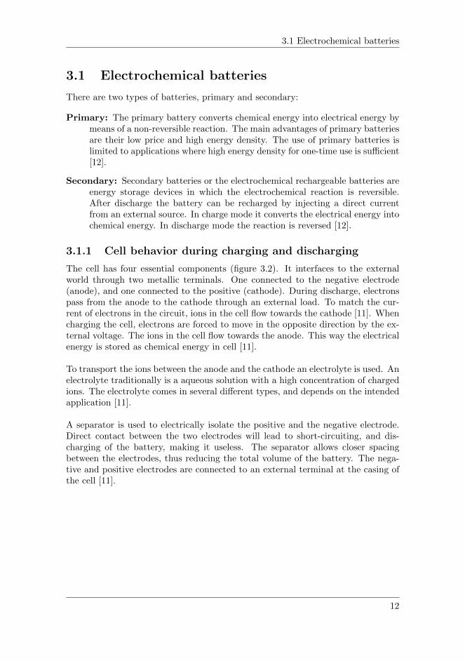
3.1.1 Cell behavior during charging and discharging

The cell has four essential components (figure 3.2). It interfaces to the externalworld through two metallic terminals. One connected to the negative electrode(anode), and one connected to the positive (cathode). During discharge, electronspass from the anode to the cathode through an external load. To match the cur-rent of electrons in the circuit, ions in the cell flow towards the cathode [11]. Whencharging the cell, electrons are forced to move in the opposite direction by the ex-ternal voltage. The ions in the cell flow towards the anode. This way the electricalenergy is stored as chemical energy in cell [11].

To transport the ions between the anode and the cathode an electrolyte is used. Anelectrolyte traditionally is a aqueous solution with a high concentration of chargedions. The electrolyte comes in several different types, and depends on the intendedapplication [11].

A separator is used to electrically isolate the positive and the negative electrode.Direct contact between the two electrodes will lead to short-circuiting, and dis-charging of the battery, making it useless. The separator allows closer spacingbetween the electrodes, thus reducing the total volume of the battery. The nega-tive and positive electrodes are connected to an external terminal at the casing ofthe cell [11].

12

Chapter 3. Energy storage devices

Figure 3.2: Essential components of a basic electrochemical cell [5].

3.1.2 Battery Terminology

Battery VoltageThe battery voltage varies with time and the level of charge. The term batteryvoltage refers to the average voltage during discharge [12].

Battery CapacityThe battery capacity represents the maximum amount of energy that can be ex-tracted from the battery under certain conditions. The battery capacity is foundby discharging the battery at a constant current until the voltage reaches a certainlimit. The most commonly used measure for battery capacity is ampere-hours (Ah)[12].

Charge/discharge voltagesThe measured terminal voltage of a cell will vary as it is charged and discharged. Inan ideal battery there would be no difference between the charge and the dischargevoltages. Both the charge and discharge curves have a plateau with little variationin voltage (figure 3.3). The average voltages in these plateaus are referred to asthe charge and discharge voltages [12].

13


Figure 3.3: Discharge and charge curves of a 1.25 V cell [12].

The Coulombic efficiencyThe coulombic efficiency is defined as the ratio between the amount of charge ex-tracted from the battery during discharge and the amount of charge which enterthe battery during charging. The value is always lower than unity [12].

ηcoulombic =Vdischarge ×AhdischargeVcharge ×Ahcharge

(3.1.1)

Self-dischargeSelf-discharge occurs for all batteries, at a rate typically below 1 % per day, butthere is some variation between different battery types. To avoid discharging atno-load conditions the battery can be trickle-charged at the same rate of the self-discharge [12].

State of chargeThe state of charge (SOC) is defined as the ratio between the charge of the batteryand the rated charge capacity. The depth of discharge (DOD), on the other handis defined as the ratio between the charge drained from the battery and the ratedcharge capacity [12].

DOD =

∫ t0idt

Q[Ah]· 100% (3.1.2)

SOC =

(1−

∫ t0idt

Q[Ah]

)· 100% = 100%−DOD (3.1.3)

Memory effectThe memory effect is a phenomenon usually seen in nickel cadmium batteries, wherethe batteries remembers the C/D pattern and changes its performance accordingly.

14


The batteries gradually lose their charge capacity when being charged, after onlybeing discharged partially [12].

3.1.3 Comparing different types of batteries

The cell stores electrochemical energy at low electrical potential typically from 1.2to 3.6 V. This mainly depends on the electrochemistry of the materials involved [12].

In the current market there exist a large variety of batteries suited for differentapplications [9]. Parameters as price, charge capacity, cell voltage, durability, andenergy density are important when choosing the battery for a given application.Figure 3.4 presents a Ragone plot of different types of batteries rated on their en-ergy to weight ratio (Wh/kg) and their energy to volume ratio (Wh/liter). As wecan see from the figure, the lithium-polymer batteries has the highest volumetricdensities, but the use is limited as a result of a high initial cost.

The Li-ion batteries are the fastest growing battery type at the moment. It hasa significantly higher volumetric energy density than many of its competitors. Italso delivers a higher cell voltage, 3.5 V per cell [12]. The energy densities rangesfrom 100 [Wh/kg] to 200 [Wh/kg] for the best Li-ion batteries. Typical ratings inpower density are between 1000 [W/kg] and 3000 [W/kg] [9].

Figure 3.4: Ragone diagram for various electrochemical batteries [12]

15

3.2 Supercapacitors

3.1.4 Batteries and cells

A battery is made up of numerous electrochemical cells connected in series, parallel,or a combination. The required battery voltage and current for a given applicationdetermines how the cells are connected. A higher output voltage is obtained byincreasing the number of cells connected in series, while a higher current is obtainedby connecting more cells in a parallel configuration [12]. The battery capacity israised by increasing the number cells.

3.2 Supercapacitors

The supercapacitor represents a relatively new type of energy storage device, eventhough the study of electrostatics and electrochemistry has been developed sincethe 17th century. Lately supercapacitors have received a significant level of inter-est for use in the electric utility industry for a variety of different applications [13].Today use of supercapacitors is found in applications such as hybrid cars, busesand trains.

As a power device, the supercapacitor currently does not possess the high en-ergy density compared to electrochemical batteries. On the other hand, they havea number of key attributes, such as the ability to charge and discharge within sec-onds, without any damage. This makes it possible to serve high power demands inshort pulse intervals. Using a battery to serve such high power pulses will result insignificant reduction of performance and life-time. Supercapacitors possess a nearlimitless recyclability with a typical life of more than 10 6 cycles. Other advantagesare environmental friendliness, low maintenance requirements, and safe operationover large temperature intervals [9].

3.2.1 Main types of supercapacitors

Supercapacitors are divided primarily by the charge mechanism and the materialsused for electrode construction. There exist three general classifications of capac-itors; electric double-layer capacitors, pseudo-capacitors, and hybrid capacitors.The electric double-layer capacitors stores energy electrostatically, the pseudo-capacitors stores energy electrochemically, while the hybrid capacitors uses a com-bination of the two mechanisms [9]. In this thesis, only the electric double-layercapacitors will be investigated further.

3.2.2 Electric double-layer Capacitors

The electric double-layer capacitors (EDLCs) are non-faradic systems. There isno transfer of charge between the electrolyte and the electrodes, in contrast to theelectrochemical battery. As a result there are no chemical or compositional changesduring charging and discharging. The lack of irreversible reactions between elec-trode and electrolyte results in a near limitless recyclability [9].

16


As explained the working principle of the EDLC involves no chemical reaction.The EDLCs consists of two electrodes, an electrolyte and two current collectors(figure 3.5). An insulating porous separator is placed between the two electrodesto avoid short-circuiting, but at the same time allow ion diffusion. When un-charged, the electrolyte consists of positive and negative ions, cations and anions.When charging the EDLC, the positive electrode attracts the anions, while thenegative electrode attracts the cations [13]. The two layers of oppositely chargedions at the interphase between the electrode and the electrolyte give rise to thedouble layer capacitance in EDLCs [9].

Figure 3.5: structure of electric double-layer capacitors [13].

Typical ratings for the EDLC in terms of power and energy density are 8000-10000[W/kg] and 3-5 [Wh/kg] respectively [9].

3.2.3 Requirements for achieving higher performance

The rated voltage of the EDLCs is determined by the oxidation potential of theelectrolyte. Electrolytes with oxidation potentials from 2.3 to 2.7 V per cell arecommon [13]. High surface area of the electrodes are important to develop thecapacitive double layer. Activated carbon is the most commonly used electrodematerial, due to its low cost and high surface area [9].

3.2.4 Performance characteristics

The capacitance C, is defined as the ratio between the stored charge Q to theapplied voltage V :

C =Q

V(3.2.1)

An important performance value is the energy density of the supercapacitor. Theenergy density of a supercapacitor directly relates to the energy stored in each

17

3.2 Supercapacitors

supercapacitor cell. Assuming that the overall capacitance and voltage potentialof the supercapacitor is known, the energy capacity of the supercapacitor is givenby [9].

E =1

2CsV

2s (3.2.2)

To serve applications that require more power than a single supercapacitor canprovide, it is necessary to stack cells. The overall capacitance and voltage potentialsof series connected cells relate to the individual cell capacitance by:

1

Cs=

1

C1+

1

C2+ .....

1

Cn→ Cs =

Cin

(3.2.3)

Vs = nVi (3.2.4)

18

Chapter 4

System Modeling

4.1 Bond graph modeling

The bond graph approach to modeling is based on identifying the energy flow ina physical system. The systems are broken down into ideal basic elements, andtheir interconnections are able to predict its behavior within reasonable accuracy.The lines between the elements represent the power flow between two ports andare called power bonds. A power bond transmits power instantaneously, with noloss. The direction of energy flow is indicated with a half arrow at the end of thepower bond [20].

Figure 4.1: Power bond

There are two variables associated with each power bond, effort (e) and flow (f ).These variables are known as power variables, and their product defines the powertransmitted between these elements [20].

P (t) = e(t)× f(t) (4.1.1)

The energy transmitted in and out of the elements is the time integral of the powervariable [20].

E(t) =

∫ t

0

P (t)dt (4.1.2)

19

4.1 Bond graph modeling

I addition to the power variables, the energy variables, momentum (p) and dis-placement (q) are useful to describe the energetic relation in a system [20]. Theenergy variables are defined as

Momentum:

p(t) =

∫ t

0

e(t)dt+ p(0) (4.1.3)

Displacement:

q(t) =

∫ t

0

f(t)dt+ q(0) (4.1.4)

These junctions can be viewed as energy switchboards, routing the energy into dif-ferent paths. The first junction is the 0-junction. This junction defines a commoneffort on all the bonds connected to the junction. The 1-junction on the otherhand, defines a common flow on all bonds connected to the junction.

There are 9 basic bond graph elements, which applies for energy storage, con-version, supply and dissipation. The table below presents the elements along withtheir constitutive relations [20].

Basic Element Mnemonic code Constitutive relationEffort source Se e=e(t)Flow source Sf f=f(t)Capacitor element C q=CeInertia Element I p=IfResistor element R e=Rf

Transformer TFe1=me2mf1=f2

Gyrator GYe1=f2rf1r=e2

0-junction 0e1=e2=e3f1-f2-f3=0

1-junction 1f1=f2=f3e1-e2-e3=0

Table 4.1: Basic bond graph elements and their constitutive relations [20].

When modeling it is important to recognize which element to use when represent-ing a given physical process. The bond graph method forms a powerful and usefultool for engineers to model dynamic systems in various energy domains.

20

Chapter 4. System Modeling

4.2 Modeling of energy storage devices

4.2.1 The Lithium ion battery

There exists multiple mathematical models that describes the charge and dischargecharacteristic of a electrochemical battery. [14] Suggests a circuit-based modelwhere the same equation is used both during charging and discharging. The modelis a modified version of the equation developed by [?], which describes the electro-chemical behavior of a battery directly in terms of terminal voltage, open circuitvoltage, internal resistance, charging current and SOC [15]. The modified modeluses only SOC as a state variable to describe the charge and discharge curves ofthe terminal battery voltage [14]. Figure 4.2 presents a typical discharge curveof a electrochemical battery. The terminal voltage is described by the followingequation:

Vt = E0 −Ri × Ib −K

(Q

Q−∫ t0idt

)+Ae(B×ti) (4.2.1)

Where:

VT - Terminal Battery Voltage [V]E0 - Constant Battery Voltage [V]Q - Battery Capacity [Ah]Ri - Internal Resistance [Ohm]∫t0idt - Actual battery charge [Ah]

A - Amplitude of exponential zone [V]B - Inverse of exponential zone time constant [Ah−1]K - Polarization constant [V]

21


Figure 4.2: Discharge characteristics of a rechargeable battery [14].

The term (Q/Q−∫t0idt) represent the non-linear change in voltage over time as the

battery is discharged with the battery current. The exponential term Ae(−B×it)

is represents the rapid voltage increase which occurs when the battery comes closeto fully charged condition [14].

The model includes some assumptions and limitations. Temperature effects, self-discharge and the battery memory effect is not included. The internal resistanceand the battery capacity are assumed to be constant, with no variations with thecurrent amplitude. The model also assumes a coulombic efficiency of 100 %, whichresults in identical charge and discharge curves [14].

The main advantage of the model is the possibility to quite accurately representthe characteristics of several different electrochemical batteries, based on data com-monly found in the manufacturers datasheet.

22


Figure 4.3: Mathematical battery model.

4.2.2 Bond graph representation of the rechargeable battery

There are several ways to model a rechargeable battery. In this thesis the modelwill be based on the mathematical representation described in chapter 4.2.

In electrical systems the power variables, flow and effort are represented by cur-rent and voltage respectively. The battery current which either charges or dis-charges the battery is modeled as a Sf -element. The internal resistance of thebattery is modeled as a R-element. The battery voltage is set by a modulatedeffort source (MSe-element), which represents equation 4.2.1. To determine theamount of charge drained from the battery a displacement sensor is placed at thebond from the current source. The 1-junction accounts for the common currentthrough the external load and the internal resistance, and a voltage drop over theinternal resistance. The bond graph representation of the battery cell is presentedin figure 4.4.

Figure 4.4: Bond graph representation of battery

23


4.2.3 Building a battery pack

By changing the parameters in the voltage equation, the model presented in figure4.4 can be used both to represent a single cell and a complete battery bank con-sisting of multiple cells. There is still some interest in showing how a single cellmodel, can be used to develop models for battery banks. As previously explainedthe battery packs achieve their desired operating voltages by connecting cells inseries. Cells connected in a parallel configuration increases the current capacity ofthe battery pack. A combination of parallel and series connected cells are used toachieve the performance requirements of the battery pack.

To model a battery pack we use the single cell model in figure 4.4 as a basis.In the battery pack model, each cell consists of the the R-element representingthe internal cell resistance, and the Mse-element which represents the cell volt-age source. In the the series branch the cells are connected by 1 -junctions, whichrepresent the voltage difference over each cell. The same amount of current runsthrough all cells in each branch, so one charge sensor is sufficient for each branch.

Figure 4.5: Bond graph representation of a battery pack.

24


4.3 The supercapacitor

A supercapacitor can easily be modeled by using some standard circuit elements.[16] Suggests the model presented in figure 4.6. The circuit model is for someproducts provided in the datasheet from the supercapacitor manufacturer EPCOS[17]. The advantage of this model is the easy determination of parameters, basedon test results or manufacturer data.

Figure 4.6: Basic conceptual model of a supercapacitor [18]

4.3.1 Parameter determination

Based on manufacturer data or experiment results the following steps should becarried out to calculate the necessary model parameters of the conceptual super-capacitor model.

During rapid change in charging current, the voltage level experiences an increasedvariation in the initial stage of the discharge process. When current suddenlypasses through the resistor, the supercapacitor experiences an additional voltagedrop, as illustrated in figure 4.7. By using the voltage drop in the initial stage ofthe discharging and the discharge current, the resistance of R1 can be determined[16]. The resistance of R1 is found by:

R1 =∆V

∆I(4.3.1)

25


Figure 4.7: Typical voltage profile for charging and discharging of a supercapacitor[19]

The main capacitance of the supercapacitor is found by using the differences incharge and voltage between two points in the voltage curve. The charge is foundas follows:

∆Q =

∫ t1

t0

idt (4.3.2)

Where i denotes the charging current. The main capacitance can then be foundby

C =∆Q

∆V(4.3.3)

or, if the energy capacity of the supercapacitor is known, the main capacitance canbe found by

C =2Q

V 22 − V 2

1

(4.3.4)

The capacitance Cp represents the effect the voltage has on the total capacitanceof the supercapacitor. [16] Suggests setting the value of Cp to be one thirteenthof C, which means that the element has a small impact on the supercapacitorsperformance.

Cp =C

13(4.3.5)

26


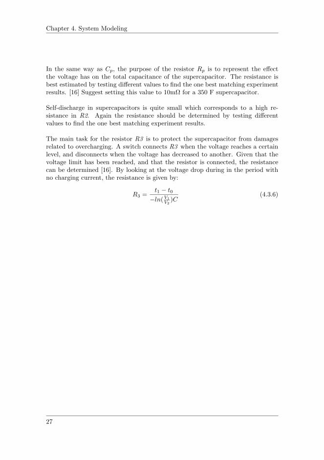
In the same way as Cp, the purpose of the resistor Rp is to represent the effectthe voltage has on the total capacitance of the supercapacitor. The resistance isbest estimated by testing different values to find the one best matching experimentresults. [16] Suggest setting this value to 10mΩ for a 350 F supercapacitor.

Self-discharge in supercapacitors is quite small which corresponds to a high re-sistance in R2. Again the resistance should be determined by testing differentvalues to find the one best matching experiment results.

The main task for the resistor R3 is to protect the supercapacitor from damagesrelated to overcharging. A switch connects R3 when the voltage reaches a certainlevel, and disconnects when the voltage has decreased to another. Given that thevoltage limit has been reached, and that the resistor is connected, the resistancecan be determined [16]. By looking at the voltage drop during in the period withno charging current, the resistance is given by:

R3 =t1 − t0−ln(V1

V2)C

(4.3.6)

27


4.3.2 Bond graph representation of the supercapacitor

The modeling of the equivalent supercapacitor circuit starts with replacing all elec-trical elements with their bond graph equivalents. Converting an electrical networkinto a non-simplified bond graph is straightforward. Nodes in the circuit are re-placed by 0-junctions. All elements and junctions are then connected according tothe layout of the electrical circuit. Figure 4.8 presents the equivalent bond graphrepresentation of the supercapacitor circuit model.

Figure 4.8: Non-simplified bond graph representation of the conceptual superca-pacitor model.

By eliminating unnecessary junctions the bond graph can simplified to the onepresented in figure 4.9. The simplified model does not present a direct symmetrywith the circuit diagram, but it indicates the flow of power from the current sourceto the other elements in a good manner. Also included in the model is the switchwhich connects the resistor R3, when the voltage reaches a certain level.Parameters of the various electrical components can now be implemented and theperformance of the supercapacitor can be simulated.

28


[H]

Figure 4.9: Simplified bond graph representation of the conceptual supercapacitorcircuit.

4.4 The three-phase inverter

The inverter is the last part of the voltage source inverter. The desired frequencyof the AC voltage is obtained by controlling the switching elements of the inverter.The three-phase inverter is build up of six switching elements which are turned onand off in a successive manner.

Figure 4.10: 3-phase transistor inverter [24].

Several methods can be used for controlling the switching of the inverter. In thisthesis, motor control is based on Direct Torque Control (DTC) which will be re-viewed in chapter 4.6. The bond graph modeling of the three-phase inverter starts

29

4.4 The three-phase inverter

with introducing an expansion of the conventional 0- and 1-junctions. This isneeded to model the ideal switching of the three identical half-bridges in the in-verter [24].

4.4.1 Switched Power Junctions

[24] defines switched power junctions (SPJs) as 0- and 1-junctions which admitsincoming effort (0-junction) or flow (1-junction) in more than one of their adjacentbonds. This will not imply a causal conflict because only one of these bonds isenabled at a given instant. The enabling and disabling of these bonds are performedby a set of control variables U1, U2, U3, ...Un. These variables take on the value of1 or 0, where only one of the variables are allowed to have the value 1 at a giventime instant. The symbols used to represent the SPJs are 0s and 1s. Figure 4.11presents generalized 0s- and 1s-junctions.

Figure 4.11: Generalized 0s- and 1s-junctions [24]

The constitutive relations of the SPJs presented in figure 4.11 can be written as

Junction effort = U1e1 + U2e2 + ...+ Unen (4.4.1)

fi = Ui(fn+1 + fn+2); i = 1, ..., n (4.4.2)

Junction flow = U1f1 + U2f2 + ...+ Unfn (4.4.3)

ei = Ui(en+1 + en+2); i = 1, ..., n (4.4.4)

30


4.4.2 Bond Graph representation of the 3-phase inverter

The modeling of the inverter unit starts with assuming that each transistor-diodepair behaves like an ideal switch. The transistor-diode pairs are represented by 1s-junctions. The 1s-junctions model the switching the current through the transistor-diode pair between the line current Ia,b,c (switch on) and 0 (switch off) [24]. The 0s-junctions models the switching of the terminal voltage between Vdc/2 and −Vdc/2which is supplied by the DC-link. The activated bonds supplies the SPJs with thecontrol variables sent from the inverter control unit (S1,S2 and S3 ). Figure 4.12presents the complete bond graph representation of the three-phase inverter.

Figure 4.12: Bond graph representation of the inverter

31

4.5 The induction motor


The induction motor or the asynchronous motor is by far the most used motor totransform the energy from the electrical domain to the mechanical in diesel-electricpropulsion systems. To simplify the modeling of the induction motor a coordinatetransformation of the three-phase currents and voltages will be performed.

4.5.1 Operating principle

In the same way as for the synchronous motor, the asynchronous motor have astator consisting of three-phase windings. The magnetic axes are shifted 120

relative to each other. The stator windings sets up a revolving magnetic field with aangular frequency determined by the network frequency. The speed of the revolvingmagnetic field is known as the synchronous speed, ωs. In the asynchronous motorthere is relative motion between the synchronous speed and the rotor speed, ωr[25]. The relative speed difference is known as slip speed, and is given by:

ωslip = sωs (4.5.1)

Where the slip, s is defined as:

s =ωs − ωrωs

(4.5.2)

Slip increases with the loading of the induction motor. When slip exists a changeof flux arises in the rotor. A electromotive force is induced, and a electrical currentis established in the short circuited windings in the rotor. These short circuitedwindings are made up of aluminum bars formed as a squirrel cage, which in turnreact with the magnetic field to produce a electromagnetic torque Tem [25].

Figure 4.13: Crossection of the induction motor (left) and the squirrel cage (right)[25].

32


4.5.2 Power invariant transformation

The dq-transformation is a mathematical transformation used to simplify the anal-ysis of both synchronous and asynchronous machines. The process of modeling theinduction motor starts with performing a dq-transformation of the 3-phase cur-rent and voltage signals sent from the inverter unit. The three-phase alternatingcomponents in the abc-frame is defined in terms of the actual winding variablesby applying the Park’s transform [26]. The new variables are obtained by project-ing the abc-components on three axes. The direct axis, the quadrate axis and thestationary axis [26].

Figure 4.14: Projection of the abc-frame on the direct, quadrate and stationaryaxis [26].

4.5.3 Mathematical description of the power invariant trans-formation

The transformation from the abc-frame to the dq-frame is mathematically expressedas

i0dq = P · iabc (4.5.3)

where the transformation matrix for the Park’s transform P is given by

P =

√2

3

1√2

1√2

1√2

cos(θ) cos(θ − 23π) cos(θ + 2

3π)−sin(θ) −sin(θ − 2

3π) −sin(θ + 23π)

(4.5.4)

33


The inverse transformation is given by

iabc = P−1 · i0dq (4.5.5)

P−1 =

√2

3

1√2

cos(θ) −sin(θ)1√2

cos(θ − 23π) −sin(θ − 2

3π)1√2

cos(θ + 23π) −sin(θ + 2

3π)

(4.5.6)

A criteria for the transformation is that the power before and after the transfor-mation is identical. If this is true, the transformation is said to be power invariant.A transformation is power invariant if the transformation matrices are orthogonal[26]. This can be confirmed by the expressions above, because PT = P−1. As aresult the power before and after the transformation should be identical.

Pabc = vaia + vbib + vcic = iabc · vTabc

=

P−1

v0vdvq

T P−1

i0idiq

=[v0 vd vq

](P−1)TP−1

i0idiq

= v0i0 + vdid + vqiq = P0dq (4.5.7)

Easier filtering and control, is one of the main advantages of performing the dq-transformation. I addition the active and reactive power can be controlled inde-pendently by controlling the dq-components.

4.5.4 Bond graph representation of the dq-transformation

The bond graph representation of the power invariant dq-transformation is modeledas suggested by [21]. This model will be used between the inverter model and themodel of the induction motor. The models input is the three-phase abc-voltages inaddition to the position angle of the rotor in the induction motor θ. The outputfrom the model is the dq-voltages. The causal strokes are assigned in such away. Six modulated TF -elements are used to represent the multiplication of thetransformation matrix. θ is used to determine the transformer modulus for all ofthe modulated TF -elements.

34


Figure 4.15: Bond graph representation if the Park’s transformation from the abc-frame to the dq-frame.

35


4.5.5 Mathematical model of the induction motor

The voltage balance for the asynchronous motor is given by the following expres-sion [21]:

v = Ri +dψ

dt(4.5.8)

Using dq-components the voltages, currents, resistances and flux linkages are givenby:

v =[vds vqs vdr vqr

]T(4.5.9)

i =[ids iqs idr iqr

]T(4.5.10)

R =

rs 0 0 00 rs 0 00 0 rr 00 0 0 rr

(4.5.11)

ψ =[ψds ψqs ψdr ψqr

]T(4.5.12)

The flux linkages are related to the inductance matrix and the dq-currents by:

ψ = Li(4.5.13)

ψdsψqsψdrψqr

=

Ls 0 Lm 00 Ls 0 LmLm 0 Lr 00 Lm 0 Lr

idsiqsidriqr

(4.5.14)

The rotor and stator current can be found by:

i = L−1ψ (4.5.15)

36


The expressions for stator and rotor current then becomes [21]:

ids =−(−Lrψds + Lmψdr)

LsLr − L2m

(4.5.16)

iqs =−(−Lrψqs + Lmψqr)

LsLr − L2m

(4.5.17)

idr =Lsψdr − LmψdsLsLr − L2

m

(4.5.18)

iqr =Lsψqr − LmψqsLsLr − L2

m

(4.5.19)

The expressions for the stator voltages, the rotor voltages and the electromechanicaltorque depends on weather we let the dq-reference frame rotate with the electricalrotor angular velocity (ωr) or synchronous speed (ωs) [21]. Letting the referenceframe rotate at electrical rotor angular velocity ωr, the voltage expressions aregiven as:

uds = rsids − ωrψqs + ˙ψds (4.5.20)

uqs = rsiqs − ωrψds + ˙ψqs (4.5.21)

0 = rridr + ˙ψdr (4.5.22)

0 = rriqr + ˙ψqr (4.5.23)

The electromechanical torque is expressed by:

Te = ψdsiqs − ψqsids (4.5.24)

The mechanical angular velocity of the rotor (ωm) is related to the electrical an-gular velocity of the rotor (ωr) by the number of pole pairs, p.

ωm =ωrp

(4.5.25)

37


4.5.6 Bond graph representation of the induction motor

The bond graph representation of the induction motor is proposed in [21], andis based on the mathematical relations presented in chapter 4.5.5. The two 1 -junctions in the upper part of the model represents equation 4.5.20 and 4.5.21. Thetransformer represents equation 4.5.25. Stator and rotor resistances are representedby R-elements and the I -fields represents equation

Figure 4.16: Bond graph model of the induction motor in the dq-frame letting thereference frame rotate with angular velocity, ωr.

38


4.6 Direct Torque Control

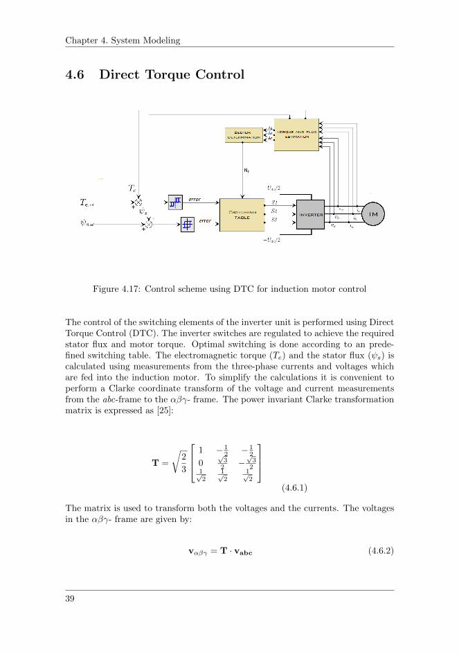
Figure 4.17: Control scheme using DTC for induction motor control

The control of the switching elements of the inverter unit is performed using DirectTorque Control (DTC). The inverter switches are regulated to achieve the requiredstator flux and motor torque. Optimal switching is done according to an prede-fined switching table. The electromagnetic torque (Te) and the stator flux (ψs) iscalculated using measurements from the three-phase currents and voltages whichare fed into the induction motor. To simplify the calculations it is convenient toperform a Clarke coordinate transform of the voltage and current measurementsfrom the abc-frame to the αβγ- frame. The power invariant Clarke transformationmatrix is expressed as [25]:

T =

√2

3

1 − 12 − 1

2

0√32 −

√32

1√2

1√2

1√2

(4.6.1)

The matrix is used to transform both the voltages and the currents. The voltagesin the αβγ- frame are given by:

vαβγ = T · vabc (4.6.2)

39


vαs =

√2

3(va − vb) +

1√6

(vb − vc) (4.6.3)

vβs =1√2

(vb − vc) (4.6.4)

vγs = 0 (4.6.5)

The currents in the αβγ- frame is given by:

iαβγ = T · iabc (4.6.6)

iαs =

√2

3(ia −

1

2ib −

1

2ic) (4.6.7)

iβs =1√2

(ib − ic) (4.6.8)

iγs = 0 (4.6.9)

The stator flux components given by

ψαs =

∫(vαs −Rsiαs)dt (4.6.10)

ψβs =

∫(vβs −Rsiβs)dt (4.6.11)

40


The magnitude of the stator flux is then determined by

ψs =√ψ2αs + ψ2

βs (4.6.12)

The electromagnetic torque Te is estimated by [21]:

Te = P (ψαsiβs − ψβsiαs) (4.6.13)

Where P is the number of poles pairs in the induction motor.

There are three variables used as input for the switching table. dT is found bycomparing the estimated electromagnetic torque with the reference torque Tref .dT = 1 calls for an increase in torque, dT = 0 indicates that the current torqueshould me maintained, while dT = −1 calls for a decrease in torque. dψ is found bycomparing the estimated stator flux with the reference value ψref . dψ = 1 meansthat an increase of stator flux is needed, while dψ = 0 means that a decrease instator flux is needed [23].

The last input variable needed for performing optimal operation of the inverterswitches is Ns. It denotes in which sector the stator flux vector is located ac-cording to the six active voltage vectors and two null vectors presented in figure4.18.

Figure 4.18: Voltage vectors [23]

The correct stator flux sector depends on the angle of the stator flux. The sectorcan be determined by using table 3.

41


A2 A1 A0 Ns

0 0 0 40 0 1 50 1 0 10 1 1 61 0 0 41 0 1 31 1 0 11 1 1 2

Table 4.2: Sector determination table [22]

The values A1, A2 and A3 is found by using the stator flux components calculatedin equation 4.6.10 and 4.6.11. The following expressions are used [21]:

A0 =

1 , |ψβs/ψαs| ≥ 1/

√3

0 , |ψβs/ψαs| < 1/√

3

A1 =

1 , ψαs > 00 , ψαs ≤ 0

A2 =

1 , ψβs > 00 , ψβs ≤ 0

The correct signals which is to be sent to the six inverter switches can now befound by using the predefined switching table. Each vector u1-u8 contains thethree switching signals S1, S2, S3.

dψ dT Ns

1 2 3 4 5 6

1 1 u2(1,1,0) u3(0,1,0) u4(0,1,1) u5(0,0,1) u6(1,0,1) u1(1,0,0)1 0 u7(1,1,1) u0(0,0,0) u7(1,1,1) u0(0,0,0) u2(1,1,1) u0(0,0,0)1 -1 u6(1,0,1) u1(1,0,0) u2(1,1,0) u3(0,1,0) u4(0,1,1) u5(0,0,1)0 1 u3(0,1,0) u4(0,1,1) u5(0,0,1) u6(1,0,1) u1(1,0,0) u2(1,1,0)0 0 u0(0,0,0) u2(1,1,1) u0(0,0,0) u2(1,1,1) u0(0,0,0) u7(1,1,1)0 -1 u5(0,0,1) u6(1,0,1) u1(1,0,0) u2(1,1,0) u3(0,1,0) u4(0,1,1)

Table 4.3: Predefined switching table [22]

The signals S1, S2 and S3 controls the on and off switching of the two switches ineach of the three identical half-bridges. In example if S1 = 1 switch 1 is on, whileswitch 4 is off.

42


4.7 DC-DC Converter

The battery and the supercapacitor is connected between the positive and thenegative side of the DC-link. The DC-link voltage is required to stay constant,which results in the need of a DC-DC converter. The DC-DC converter ensures thatthe output voltage from the energy storage devices matches the voltage level of theDC-bus. Though DC-DC converters in reality are controllable electrical circuits,the DC-DC converter is simply modeled as a MTF -element. The transformermodulus is expressed as

m =VTVDC

(4.7.1)

4.8 The propeller

The propeller has the inertia Jp and is loaded by the torque Tp. The inertia isrepresented by an I -element. In the model, a single I -element accounts for thepropeller inertia, the rotor inertia and the inertia of the propeller shaft. The loadtorque Tp is represented by an R-element and is typically expressed by

Tp = K ∗ ω2p (4.8.1)

where K is a constant, and ωp represents the propeller speed.

A simplified representation of wave disturbances can easily be added to the modelby adding a time dependent sinusoidal term. Thus the new expression for the loadtorque is given by

Tp = K · ω2p(1 +A · sin

(2πt

T

)) (4.8.2)

where A determines the amplitude if the sinusoidal term and T is the wave period.

43

4.9 Power flow control

4.9 Power flow control

The power flow of the system is said to follow the law of energy conservation. Thepower consumed by the load should be equal to the power supplied by the powersources. The relationship between the power generated by the source (Psource), thepower consumed by the load (Pload), and the power flow from the energy storagedevices (PESD) is expressed as

Psource = Pload + PESD (4.9.1)

where

PESD = PB + PSC (4.9.2)

The expression above is used to calculate the charging current of the energy storagedevices (ESDs). The ESDs can act as a load, as well as a source of power, dependingon the direction of the power flow. To determine when to charge and discharge theESDs, it is necessary to determine a limit for the power which should supplied bythe generator, PG,lim. Should the power demand of the load be higher than PG,lim,the ESDs will deliver power in combination with the generator. Should the powerdemand from the load be lower than PG,lim, power from the generator can be usedto charge the ESDs. This way the load demand fluctuations seen by the generatoris reduced. PG,lim should be set to the operating point where the fuel efficiencyof the diesel engine is at its maximum. If the ESDs both become discharged, thepower limitation should be ignored and additional generators should be connectedto the power grid if necessary.

Figure 4.19: Charging and discharging during load variations.

The direction and amount of current flowing between the ESDs and the DC-gridis determined by

IESD =Psource − Pload

VDC(4.9.3)

44


In the model the desired charging current is obtained by controlling the resistancein a R-element. The resistance of the R-elements is given by

RESD =VDCIESD

(4.9.4)

4.9.1 SOC and voltage limitations

To ensure safe operation of the ESDs some limitations are defined in the proposedenergy management system. The first limitation to consider is the state of charge(SOC). The terminal voltage (VT ) of the battery will decrease during discharge.This will increase the current drawn from the battery to provide a constant poweroutput. As a result the system rating will increase and there is a risk of overheatingthe battery. Discharging the battery to low SOC values are also not recommendeddue to the related shortening of its cycle life. Lower limits for the value of SOC istherefore required. As the upper limit for the value of SOC is 100%, overchargingthe battery will not be possible.

The maximum supercapacitor voltage is equal to the DC-voltage of the network.

45

4.10 The complete power plant

4.10 The complete power plant

To investigate the behavior of the power plant all the component must be connected.Two Se-elements will be used to represent DC-bus voltages Vdc/2 and Vdc/2. TheSe-elements will serve as the power input to the system. The model for the completepower plant is presented in figure 4.20.

Figure 4.20: Complete system model.

46

Chapter 5

Results

Before the simulations can be carried out several parameters needs to be specified.The induction motor chosen for the simulations has a rated power output of 200[kW], which will serve as a basis when assuming the rest of the model parameters.The procedure for determining the induction motor parameters can be found inappendix A, along with the values used in the model. Key model parameterswill be specified with their corresponding simulation plots, while the remainingparameters can be found in appendix B along with the source code from 20-sim.

5.1 Simulation energy storage performance

5.1.1 The battery pack

The battery is assumed to possess a charge capacity of 79.5 [Ah], a energy capacityof 7.6 [kWh] and a average battery voltage of 96 V. The parameter values are setto manipulate a typical discharge curve of a Li-ion battery. Table 5.1 presents allmodel parameters and their assumed values.

Parameter Sign ValueBattery constant voltage E0 96 VBattery Capacity Q 79.5 [Ah]Polarization constant K 3.5 [V]Amplitude of exponential zone A 7[V]Inverse of exponential zone time constant B 0.0002[Ah−1]Internal resistance Ri 0.01[Ω]

Table 5.1: Model parameters for the battery model

Figure 5.1 presents the simulation results of a complete discharge of the lithium-ionbattery. The discharge current is set to 100 [A].

47

5.1 Simulation energy storage performance

Figure 5.1: Discharge curve of the battery, Ib = −100[A].

5.1.2 Supercapacitor

The model parameters of the supercapacitor is determined by first assuming that itsenergy capacity is 5% percent of battery energy capacity. The maximum allowedsupercapacitor voltage is chosen to be the same as the bus voltage. The maincapacitance is then found by equation 4.3.4. All model parameters are given intable 5.2. The resistance R

Component R1[Ω] R2[Ω] R3[Ω] Rp[Ω] C[F] Cp[F ]Value 0.08 2000 10 0.01 4.2930 0.3302

Table 5.2: Model parameters for the supercapacitor

A complete charge-discharge cycle is presented in figure 5.2. The charging currentis set to 300 [A] until the voltage reaches 800 [V], then the charging current is set to0 [A] for 10 seconds until the supercapacitor is completely discharged by a currentof 300 [A].

48

Chapter 5. Results

Figure 5.2: Simulation result of a complete charge-discharge cycle of the superca-pacitor.

5.1.3 Discussion

The plots presents the typical performance properties in a good way. Figure 5.1shows the rapid voltage increase which occurs when the battery is fully charged.Figure 5.2 indicated the voltage variations when the charging current is changed.Over the 10 seconds the charging current was set to 0 [A], the self-discharge isnegligible.

49

5.2 Case simulations


Two case simulation are carried out to demonstrate the use of the model. Duringthe first case the load fluctuations are rapid, similar to what is typical during DP-operation. Here the supercapacitor will be used as the energy storage device, dueto its ability to serve sudden power demands during fast charging and dischargingwithout any damage. In the second simulation the period of the power fluctuationsare longer, and the battery will be used for energy storage. Such operation profilescan be relevant for tugboats and for platform supply vessels during maneuveringand DP-operation. The two effort sources supplies the inverter with 400 [V] on thepositive side and -400 [V] on the negative side for both case simulations. PG,lim ischosen to be 150 [kW].

5.2.1 Case 1 - DP-operation with supercapacitor

In case 1 the reference torque follows a sinusoidal curve with a period of 5 seconds,the amplitude is set to 550 [Nm] and the average value is 900 [Nm].

The resistance R3 is removed from the supercapacitor model (chapter 4.3) duringthe case simulation since the task of preventing the supercapacitor from overcharg-ing is carried out by the energy management system.

Figure 5.3 presents the load sharing between the source and the supercapacitorduring the fluctuating load demand. The resulting supercapacitor voltage is shownin the middle plot, while the corresponding current is displayed in the lower plot.Positive current is equivalent to charging the supercapacitor.

The two plots in figure 5.4 presents the electromagnetic torque and the propellerspeed.

50

Chapter 5. Results

Figure 5.3: Load sharing, supercapacitor voltage and charging current.

Figure 5.4: Propeller speed and electromagnetic torque

51


5.2.2 Comments to case 1

The results in figure 5.3 confirms that during low load conditions the current to thesupercapacitor is positive and voltage increases as the supercapacitor is charged.During high load conditions on the other hand, current is drawn from the super-capacitor and the voltage decreases as it discharges. As a consequence, the powersupplied by the power source remains constant. The load disturbances of the powerplant is thereby reduced which facilitates for stable operation of the generator set.

A criteria for the reducing the load fluctuations seen by the diesel engines is thatthe supercapacitor voltage is kept within its limits.

Rapid variations of the electromagnetic torque produced by the DTC controllercan be seen in figure 5.3. The level of variation is significantly reduced by decreas-ing the simulation time step. As a result, a trade-off between simulation time andlevel of torque variations was necessary.

5.2.3 Case 2 - Operation with a battery pack

Case 2 simulates the system performance while using the battery for energy storage.The reference torque was varied according to table 5.3. The lower and upper SOC-limitation was set to 40 %and 100 % respectively.

Time [s] Tref [Nm]0 - 30 130030 - 60 150060 - 100 1000100 - 140 1550140 - 170 1050170 - 200 1350200 - 220 750220 - 270 1600270 - 300 1000

Table 5.3: Reference torque

The load sharing between the source and the battery during varying load demandis presented in the first plot of figure 5.5. The middle plot shows the resulting SOCcurve, while the lower plot presents the charging current. Positive current meansthat the battery is charged.

Figure 5.6 displays the electromagnetic torque of induction motor rotor in thetop plot. The corresponding propeller speed can be seen in the lower plot.

52

Chapter 5. Results

Figure 5.5: Load sharing, SOC and charging current from case simulation 2.

Figure 5.6: Propeller speed and electromechanical torque.

53


5.2.4 Comments to case 2

In the same way as for case 1, the results from case 2 show that while the loadis below the power limitation of the source the battery is charged, the state ofcharge increases and the current to the battery is positive. While the load is abovethe power limitation of the source the battery is discharged, the state of chargedecreases and the charging current in negative. As a result the load profile seen bythe power source stays almost constant. During the first 10 seconds of the simula-tion, Pload is below PG,lim, but there still is no power consumed for charging thebattery. This is a result of the battery initially being fully charged and the energymanagement system protecting it from overcharging.

The wave disturbances on the propeller is transmitted to back to the DC-bus andthe effect is visible in several plots. Because the battery acts as a energy buffer,the disturbances will influence the operational conditions of the prime mover.

In the same way as for case 1 there exist rapid variations of the electromagnetictorque of the rotor in the induction motor. The level of variations is increasedcompared to case 1, mainly due to a larger time step in the simulation.

54

Chapter 6

Conclusions andrecommendations

The current development in marine power systems suggest that hybrid technologywill be found in an increasing number of applications in the years to come. Contin-uously improvements in the energy storage technology improves the potential foreconomical benefits as well as environmental. Stricter environmental regulationsand increasing fuel prices will boost the hybridization of the marine industry in theyears to come.

The review of the two energy storage concepts in chapter 3 revealed significantdifferences in performance properties. Of the different battery types, the Li-ionbattery is the most promising, because of its low-price and its high energy density.Compared to supercapacitors a typical Li-ion battery has the ability to store 20- 40 times more energy per unit weight, while the supercapacitor can supply 3-10times more power. The most beneficial solution is obtained with both devices em-bedded in the same system and optimizing their interaction based on their differentperformance properties and limitations.

The bond graph method used for the component modeling proved to be helpfulby its ability to indicate the energy flow and causality in electric power systems.

The most important aspect of the produced results is that they confirm the modelsability to demonstrate the system behavior as expected. Considering its limitationsthe model depicts the basic principles of a hybrid marine power plant. The peakshaving effect from the power source point of view is can easily be identified. Onthe other hand the models accuracy can not be verified without comparing theresults with test measurements. The model parameters used for the energy stor-age components has great influence on the systems behavior. Their chosen valuesproved to generate the performance results one should expect.

55

6.1 Recommendations for further work

6.1 Recommendations for further work

Hybrid power plants are complex systems and encounters multiple engineeringdisciplines. Some of the most obvious expansions and features which should bepursued are listed below.

• Development and implementation of component models of generators anddiesel engines. Differences in fuel consumption and emissions with and with-out energy storage can then be estimated.

• Development of tools for temperature monitoring and life-time estimation ofthe energy storage devices.

• Implementation of sufficient control strategies for power control and systemoptimizing for fuel efficiency and emissions.

• Verification of the complete model should be carried out, through testing andfull-scale measurements.

• Modeling of more realistic environmental loads for different scenarios.

56

Bibliography

[1] Alf Kare Adnanes. Marine Electrical Installations And Diesel Electric Propul-sion. ABB Marine, 2003.

[2] Diesel-electric Propulsion Plants, A brief guideline how to engineer a diesel-electric propulsion system . MAN.

[3] Cummins Inc. Meeting the Next Challenge, IMO Tier II and III . 5 - 2011.

[4] DNV Research and Innovation. Fuel Cells for Ships. Position Paper 13-2012.

[5] Jack Erjavec. Hybrid, Electric and Fuel-Cell Vehicles . 2nd Edition, 2013.

[6] Siemens Innovation News. First Car Ferry Powered by Electric Drive System.2013.

[7] Rakopoulos, Constantine D., Giakoumis, Evangelos G. Diesel Engine TransientOperation. Springer-Verlag London Limited, 2009.

[8] Jan F. Hansen, John O. Lindtjørn and Klaus Vanska. Onboard DC-Grid forenhanced DP operation in ships. ABB, Dynamic Positioning Conference 2011.

[9] Ru-Shi Liu, Lei Zhang, Xueliang Sun, Hansan Lui and Jiujun Zhang. Electro-chemical Technologies for Energy Storage and Conversion.Wiley-VCH, Volume1, 2012.

[10] R. Kotz and M. Carlen. Principles and applications of electrochemical capaci-tors. Electrochimica Acta 45(15-16): 2483-2498, 2000.

[11] Technical Marketing Staff of Gates Energy Products, Inc. Rechargeable batter-ies, Applications Handbook, Elsevier, 1998.

[12] Mukund R. Patel. Shipboard electrical Power System. CRC Press, 2012.

[13] Stanley Atcitty. Electrochemical Capacitor Characteization for Electric UtilityApplication. Virginia Polytechnic Institute and State University, 2006.

[14] Olover Trembley, Louis-A. Desaint, Abdel-Illah Dekkiche. A Generic BatteryModel for the Dynamic Simulation of Hybrid Electric Vehicles.Ecole de Tech-nologie Supericure, Electric Engineering Department, 2007.

57

BIBLIOGRAPHY

[15] C. M. Shepherd. Design of Primary and Secondary Cells - Part 2. An equationdescribing battery discharge. 1965.

[16] C. Farcas, D. Petreus, I. Ciocan and N. Palaghita. Modeling and Simulationof Supercapacitors. 2009.

[17] Data sheet for supercapacitor from EPCOS. Part. No.: B48621-S0203-Q288.

[18] Patrik Johansson and Bjorn Andersson, Comparison of Simulation Programsfor Supercapacitor Modelling. Model Creation and Verification, Chalmers Uni-versity of Technology,2008.

[19] Monzer Al Sakka, Hamid Gualous, Noshin Omar and Joeri Van Mierlo, Bat-teries and Supercapacitors for Electric Vehicles. 2012.

[20] Eilif Pedersen and Hallvard Engja. Mathematical Modelling and Simulation ofPhysical Systems. Department of Marine technology, Norwegian University ofScience and Technology, 2010.

[21] Tom Arne Pedersen. Bond Graph Modeling of Marine Power Systems. Doc-toral thesis, Department of Marine technology, Norwegian University of Scienceand Technology, 2009.

[22] Bibhu P. Panigrahi, Dinkar Prasad and Sabyasachi SenGupta A simple hard-ware realization of switching table based direct torque control of induction mo-tor”, 2007.

[23] Giuseppe Buja and Marian P. Kazmierkowski. Direct torque control methodsfor voltage source inverter-fed induction motors - A review”, 2003.

[24] Sergio Junco and Alejandro Donaire. Bond Graph Modeling and Simulation ofEngineering Systems. Springer Science + Business Media, LLC 2011.

[25] Slobodan N. Vukosavic. Electrical Machines. Springer New York, 2013.

[26] P. M. Anderson and A. A. Fouad Power System Control and Stability. TheIowa State University Press. Ames, Iowa. 1st edition, 1977.

58

Appendices

i

Appendix A

Parameter Calculation forthe Induction motor

Data provided by the induction motor manufacturer is presented in the table below:

Rated output 200 kWLine voltage 400 VFrequency 50 HzPoles 4Rated speed 1486 RPMMoment of inertia 3.5 kgm2

Connection ∆/DeltaPowerfactor (100% loading) 0.86

Table A.1: Data for the induction motor, Type: M3BP 315MLA 4 IMB35/IM2001

To extract the parameters needed in the model, test results from the manufacturersdata sheet where used. The parameter calculations are based on the per-phaseequivalent circuit diagram of the induction motor suggested by [25].

A.1 No-load test

During the test the rotor is unblocked and allowed to run uncoupled from anymechanical load at rated voltage and frequency. The input current, voltage andpower is measured in addition to core losses, winding losses and friction. When themotor is uncoupled from any mechanical load the rotor revolves with no externalresistance. The load torque is zero and mechanical losses are negligible in mostcases. As a result the relative slip is close to zero and the rotor rotates at almostsynchronous speed, ns. The rotor resistance R2 becomes so large that the rotorcurrent is negligible and the equivalent circuit diagram reduces to a series con-

ii

Chapter A. Parameter Calculation for the Induction motor

Figure A.1: Equivalent per-phase circuit for an induction motor

nection of the stator resistance Rs, the stator reactance Xs and the magnetizingreactance Xm [25]. The equivalent no-load circuit is presented in figure A.2.

Figure A.2: Equivalent per-phase circuit of the induction motor during No-loadtest

Power input, PNL 3.14 kWLine, voltage, Vl 399.8 VFrequency, f 50 HzLine current, Il 111.8 APower factor, p.f 0.04Speed, n 1500 RPM

Table A.2: Results from No-load test

The expressions for the no-load impedance, resistance and reactance depends onthe type of connection configuration. For a delta connected induction motor the

iii

A.1 No-load test

expressions are given by:

No-load impedance:

ZNL =Vl√

3

Il=

399.8 ·√

3

111.8= 6.194[Ω] (A.1.1)

No-load resistance:

RNL =PNLI2l

=3.14 ∗ 103

111.82= 0.2512[Ω] (A.1.2)

No-load reactance:

XNL = X1 +XM =√Z2NL −R2

NL =√

6.1942 − 0.25122 = 6.189[Ω] (A.1.3)

iv


A.2 Blocked rotor test

In the blocked rotor test, both the rotor and the stator currents has the line fre-quency. The rotor is blocked, resulting an a slip equal to unity. The equivalentper-phase circuit reduces to a series connection consisting of the stator resistanceRs, the stator reactance Xs, the rotor reactance X2 and the rotor resistance R2

[25].

Figure A.3: Equivalent per-phase circuit of the induction motor during the blockedrotor test.

Power input, PBL 13.5 kWLine, voltage, Vl 71.9 VFrequency, f 50 HzLine current, IBL 351.6 APower factor, cos(φ) 0.31Speed, n 0 RPM

Table A.3: Results from blocked rotor test

The blocked rotor resistance is found by:

RBL =PBLI2l

= 0.1092[Ω] (A.2.1)

Assuming that R1 is half of RBL gives:

R1 = 0.5460[Ω] (A.2.2)

The rotor resistance if found by subtracting the stator resistance from the totalresistance measured during the blocked rotor test.

v

A.2 Blocked rotor test

R2 = RBL −R1 = 0.1092− 0.05460 = 0.05460[Ω] (A.2.3)

ZBL =Vl√

3

Il=

71.9 ·√

3

351.6= 0.3541[Ω] (A.2.4)

XBL =√Z2BL −R2

BL =√

0.35412 − 0.10922 = 0.3369[Ω] (A.2.5)

To find the blocked rotor reactance we assume that the ratio between rotor and sta-tor reactance is equal to 1.35, which is a reasonable value for this type of inductionmotor [21].

XBL = X1 +X2 = X1 +1

1.35X1 (A.2.6)

Which gives

X1 =1.35

2.35·XBL = 0.1935[Ω] (A.2.7)

X2 =1

1.35·X1 = 0.1433[Ω] (A.2.8)

The magnetizing reactance:

Xm = XNL −X1 = 6.189− 0.1935 = 5.995[Ω] (A.2.9)

All parameters of the equivalent per-phase circuit is presented in table A.4.

Stator resistance R1 0.0546 [Ω]Rotor resistance R2 0.0546 [Ω]Stator reactance X1 0.1935 [Ω]Rotor reactance X2 0.1433 [Ω]Magnetizing reactance Xm 5.9950 [Ω]

Table A.4: The parameters of the equivalent per-phase circuit for the inductionmotor

vi


A.3 Calculation of inductance parameters and ro-tational losses

For a delta-connected induction motor the following relations are valid:

Vrms = Ul = 400[V ] (A.3.1)

Irms =Il√3

=352.1√

3= 203.3[A] (A.3.2)

Vref =√

2Urms =√

2 · 400V = 565.7[V ] (A.3.3)

Iref =√

2Irms =√

2 · 203.3 = 287.5[A] (A.3.4)

Zref =VrefIref

=565.7

287.5= 1.967[Ω] (A.3.5)

Lref =Zrefωr

=565.7

2π · 50= 0.006263[H] (A.3.6)

The per unit values (p.u.) for the inductances can now be calculated by:

Lspu =Xs

Zref=X1 +Xm

Zref= 3.145 (A.3.7)

Lrpu =Xr

Zref=X2 +Xm

Zref= 3.120 (A.3.8)

Lmpu =Xm

Zref= 3.406 (A.3.9)

The actual inductances are is expressed by:

Ls = LspuLref = 0.01970[H] (A.3.10)

Lr = LrpuLref = 0.01954[H] (A.3.11)

vii

A.3 Calculation of inductance parameters and rotational losses

Lm = LmpuLref = 0.01908[H] (A.3.12)

The rotational losses on the mechanical side of the induction motor can be foundusing the results form the no-load test. Subtracting the stator copper losses fromthe no-load power will give us the rotational power loss.

Prloss = PNL − 3I2sR1 = 2.457[kW ] (A.3.13)

The relation between the friction torque and the rotational speed is assumed to benon-linear. The friction torque is expressed by:

Tfric = Cfric(ω

ωr)0.1 (A.3.14)

where the rated angular motor speed, ωr is found by:

ωr =2πf

P=

2π · 50

2= 157.08[rad/s] (A.3.15)

Cfric, represents the friction coefficient, and is determined by:

Cfric =Protωr

= 15.6417[Nm] (A.3.16)

viii


A.4 Test report of the induction motor

ix

Appendix B

Source code from 20-Sim

This appendix presents the code from 20-sim for the main components.

B.1 Mse, battery

B.2 SOC-Calculator

x

Chapter B. Source code from 20-Sim

B.3 Torque and flux determination

xi

B.4 Switching table

B.4 Switching table

xii


xiii

B.4 Switching table

xiv


B.5 Sector determination

B.6 1s-junction

xv

B.7 0s-junction

B.7 0s-junction

B.8 Rotor and propeller inertia

B.9 Propeller load

xvi


B.10 TF, induction motor

B.11 I, rotor and stator current

xvii

B.12 Rotational losses

B.12 Rotational losses

xviii

modeling of hybrid marine electric propulsion systems

Documents