modeling of horns and enclosures for loudspeakers
TRANSCRIPT

HAL Id: tel-01546159https://hal.archives-ouvertes.fr/tel-01546159
Submitted on 8 Jul 2017
HAL is a multi-disciplinary open accessarchive for the deposit and dissemination of sci-entific research documents, whether they are pub-lished or not. The documents may come fromteaching and research institutions in France orabroad, or from public or private research centers.
L’archive ouverte pluridisciplinaire HAL, estdestinée au dépôt et à la diffusion de documentsscientifiques de niveau recherche, publiés ou non,émanant des établissements d’enseignement et derecherche français ou étrangers, des laboratoirespublics ou privés.
Modeling of Horns and Enclosures for LoudspeakersGavin Putland
To cite this version:Gavin Putland. Modeling of Horns and Enclosures for Loudspeakers. Acoustics [physics.class-ph].University of Queensland, 1996. English. tel-01546159

Modeling ofHorns and Enclosures
for Loudspeakers
byGavin Richard Putland, BE (Qld)
Department of Electrical and Computer EngineeringUniversity of Queensland
Submitted for the degree of Doctor of PhilosophyDecember 23, 1994
Revised November 1995
Accepted February 6, 1996
Examiners:
Dr. John T. PostKlipsch Professional,Hope, Arkansas, USA;
Prof. H. HolmesDept. of Electrical Engineering
University of New South Wales, Australia;
Dr. N. ShuleyDept. of Electrical & Computer Engineering
University of Queensland, Australia.
Supervisor: Dr. L.V. Skattebol.

ii
To my parents,
Frank and Del Putland

Acknowledgments
My interest in horn theory was inspired by Dr E.R.Geddes, whose paper “AcousticWaveguide Theory” [18] raised the questions addressed in Chapters 3 to 5 of thisthesis, suggested some of the answers, and provided many of the related references.These debts are not diminished by my disagreement with Geddes’ analysis of theoblate spheroidal waveguide, which he subsequently revised [19]. My paper on one-parameter waves and Webster’s equation [43] was improved as a result of a personalcommunication from Dr Geddes (October 10, 1992), which alerted me to the exis-tence of Fresnel diffraction fringes within the coverage angles of finite horns at highfrequencies.
I wish to thank the Executive Editor and Review Board of the Journal of theAudio Engineering Society for their patient handling of the complex exchange ofcorrespondence that followed my “Comments on ‘Acoustic Waveguide Theory’ ” [42].
I am indebted to an anonymous reviewer of my article “Acoustical Properties ofAir versus Temperature and Pressure” [44] for correcting my explanation of the effectof humidity on absorption, and for drawing my attention to ANSI S1.26-1978 [41],which is cited frequently in the final version of the article and in Chapter 9.
My supervisor, Dr Larry Skattebol, provided critical feedback on my three publi-cations and on numerous partial drafts of this thesis. I thank him for his flexibility inaccepting my research proposal, and for his subsequent prudence in curbing my ten-dency to pursue new lines of inquiry; without his guidance, this already protractedproject would have taken considerably longer. I also thank Prof. Tom Downs andDr Nick Shuley, colleagues of Dr Skattebol in the Dept. of Electrical and ComputerEngineering, University of Queensland, for their comments on reference [42].
The Italian text of Somigliana’s letter [51] (paraphrased in Appendix A) wastranslated by Br. Alan Moss, who was then a graduate student in the Departmentof Studies in Religion, University of Queensland.
The Japanese text of Sections 1 to 3 of Arai’s paper [2] was translated by AdrianTreloar of the Department of Japanese and Chinese Studies, University of Queens-land.
The titles and authors of the major public-domain software used in this projectare as follows. Equivalent circuit simulations were performed using SPICE3 by TomQuarles, with the nutmeg user interface by Wayne Christopher. Programs werecompiled by the GNU project C compiler. Most diagrams were drawn using xfigby Supoj Sutanthavibul et al., converted to LATEX picture commands using fig2devby Micah Beck et al., and finally edited as text files. All source files were editedwith jove by Jonathan Payne, and spell-checked with ispell by Pace Willisson etal. This document was typeset and printed within the Department of Electrical andComputer Engineering, University of Queensland, using LATEX2ε by Leslie Lamport.
This project was supported by an Australian Postgraduate Research Award.
iii

Statement of Originality
I declare that the content of this thesis is, to the best of my knowledge and belief,original except as acknowledged in the text and footnotes, and that no part of it hasbeen previously submitted for a degree at this University or at any other institution.
In a thesis drawing on such diverse subjects as mechanics, thermodynamics,circuit theory, differential geometry, vector analysis and Sturm-Liouville theory, theauthor must make exaggerated efforts to maintain some theoretical coherence. Thismay involve deriving well-known results in a manner appropriate to the context;examples include the hierarchy of forms of the equations of motion and compression(Chapter 2), and the derivation of admittances and Green’s functions from Webster’sequation (Chapter 3). Furthermore, when a thesis contains results at variance withearlier results in the literature, the author will be expected to justify his findings withexceptional thoroughness. In particular, he may be obliged to conduct mathematicalarguments at a more fundamental level than would normally be appropriate; anexample is my detailed solution of the heat equation to determine the basic thermaltime constant of the air-fiber system (Chapter 8). In such cases, the context willindicate that the result is included for the sake of clarity, cohesion or rigor, and notnecessarily because of novelty.
To avoid excessive reliance on “the context”, I offer the following summary ofwhat I believe to be my principal original contributions and their dependence onthe work of earlier researchers. This summary also serves as an extended abstract.
• In Chapter 2, I have shown how the numerous familiar equations related tothe inertia and compliance of air can be understood as alternative forms oftwo basic equations, which I call the equations of motion and compression.The hierarchy of forms eliminates redundancy in the derivations and clearlyshows what simplifying assumptions are involved in each form. The “one-parameter” or “1P” forms apply when the excess pressure p depends on asingle spatial coordinate ξ, which measures arc length normal to the isobaricsurfaces. These forms are expressed with unprecedented generality, and arecritical to the mathematical argument of subsequent chapters. Other formslead to the familiar electrical analogs for acoustic mass and compliance (bothlumped and distributed).
• After a review of previous literature, I have shown that the “Webster” hornequation, which is usually presented as a plane-wave approximation, followsexactly from the 1P forms of the equations of motion and compression, withoutany explicit assumption concerning the wavefront shape. The ξ coordinate isthe axial coordinate of the horn while S(ξ) is the area of a constant-ξ surfacesegment bounded by a tube of orthogonal trajectories to all the constant-ξsurfaces; such tubes (and no others) are possible guiding surfaces.
iv

v
• I have shown that the Helmholtz equation admits solutions depending on asingle spatial coordinate u if and only if |∇u| and ∇2u are functions of u alone.The |∇u| condition allows u to be transformed to another coordinate ξ, whichmeasures arc length along the orthogonal trajectories to the constant-ξ sur-faces. Hence, in the definition of a “1P” pressure field, the normal-arc-lengthcondition is redundant. Using an expression for the Laplacian of a 1P pres-sure field, I have shown that the wave equation reduces exactly to Webster’sequation; this is a second geometry-independent derivation. I have also shownthat the term “1P acoustic field” can be defined in terms of pressure, velocitypotential or velocity, and that all three definitions are equivalent.
• I have expressed the 1P existence conditions in terms of coordinate scale fac-tors and found that in the eleven coordinate systems that are separable withrespect to the Helmholtz equation, the only coordinates admitting 1P solutionsare those whose level surfaces are planes, circular cylinders and spheres (Chap-ter 5). Geddes [18] reported in 1989 that Webster’s equation is exact in thesame list of coordinates, but did not make the connection between Webster’sequation and 1P waves.
• Without using separable coordinates, Somigliana [51] showed that there areonly three 1P wavefront shapes allowing parallel wavefronts and rectilinearpropagation; the permitted shapes are planar, circular-cylindrical and spheri-cal. I have shown (Chapter 5) that the conditions of parallel wavefronts andrectilinear propagation are implicit in the 1P assumption, so that the threegeometries obtained by Somigliana are the only possible geometries for 1Pwaves. This result has the practical implication that no new 1P horn geome-tries remain to be discovered.
• I have produced an annotated paraphrase, in modern notation, of Somigliana’sproof (Appendix A), and adapted his proof so as to take advantage of the1P existence conditions (Chapter 5). In the theorems of Chapter 5 and thefootnotes to Appendix A, I have filled in several missing steps in Somigliana’sargument. I found it most convenient to prove these results independently,although related results exist in the literature on differential geometry.
• Working from the permitted 1P wavefront shapes and the exact derivations ofWebster’s equation, I have given wide conditions under which that equation isapproximately true, so that traditional approximate derivations of the equationcan be replaced by the more general 1P theory.
• I have extended the finite-difference equivalent-circuit (FDEC) method pro-posed in 1960 by Arai [2]. In Chapter 6, I have shown that a finite-differenceapproximation to Webster’s equation yields the nodal equations of an L-Clatter network (confirming Arai’s unproven assertion that his one-dimensionalmethod can be adapted for horns), while a similar approximation to the waveequation in general curvilinear orthogonal coordinates yields the nodal equa-tions of a three-dimensional L-C network. I have obtained the same circuitsfrom the equations of motion and compression in order to show that “current”in the equivalent circuit is volume flux, as expected. I have shown how thenetwork should be truncated at the boundaries of the model and terminatedwith additional components to represent a range of boundary conditions.

vi STATEMENT OF ORIGINALITY (WITH EXTENDED ABSTRACT)
• Arai suggested that fibrous damping materials could be handled by using com-plex values of density and bulk modulus for the air. In Chapter 7, I havederived expressions for complex density and “complex gamma” (related tocomplex bulk modulus) and shown how these quantities can be represented byintroducing additional components into the equivalent circuit.
• An equivalent circuit for a fiber-filled bass enclosure was given by Leach [30]in 1989. Leach’s derivation does not use the finite-difference method, is lessrigorous than mine (especially in its treatment of compliance), makes differentassumptions in the determination of complex density, does not use any conceptrelated to complex bulk modulus, does not use the most appropriate definitionof the thermal time constant (as Leach himself acknowledges), and does notfully explore the relationships between the possible definitions (the value of thetime constant depends on what conditions are held constant during the heattransfer). In Chapter 7, I have defined five different thermal time constants, ofwhich one is useful for deriving the complex gamma and another (which I call“basic”) is easier to calculate from the specifications of the damping material.I have shown that two of the five time constants can be read off the equivalentcircuit, and hence expressed all the time constants in terms of the “basic” one,denoted by τfp, which is the time constant at constant fiber temperature andconstant pressure.
• Values of τfp found by Leach [30] and Chase [14] are extremely inaccurate, andneither author gives a convenient method of calculating the time constant forarbitrary fiber diameters and packing densities. In Chapter 8, I have rectifiedthese deficiencies by reworking the solution of the heat equation (finding theerror in Leach’s analysis) and fitting an algebraic formula to the results. Theformula is
τfp ≈d2
8α(m2 −m0.37) ln
(
m+12
)
where d is the fiber diameter, α is the thermal diffusivity of air, f (not inthe formula) is the fraction of the overall volume occupied by the fiber, andm = f−1/2.
• Chapter 9 gives some simple algebraic formulae for calculating α and otherrelevant properties of air from the temperature and pressure. This chapter ismostly a compilation of results from the literature; my only original contribu-tions are some simple curve-fitting and a discussion of errors.
• In Chapter 10, using the results of Chapters 6 to 9, I have constructed a two-dimensional finite-difference equivalent-circuit model to predict the frequencyresponse of a moving-coil loudspeaker in a fiber-filled box. The model incorpo-rates an equivalent circuit of a moving-coil driver, which I have modified so asto allow the diaphragm to span several volume elements in the interior of thebox. Unlike conventional equivalent-circuit models of loudspeakers, this modelallows for spatial variations of pressure inside the box and shows the effectsof internal resonances on the frequency response. By observing the effects ofomitting selected components from the model, I have found that viscosity isthe dominant mechanism of damping and that, in the cases considered, thepredicted response is not greatly altered by assuming thermal equilibrium. The

vii
latter finding diminishes the significance of, but depends on, the calculationof the thermal time constant.
• In Chapter 11, I have illustrated and validated the FDEC representation ofa free-air radiation condition in curvilinear coordinates, by applying it to theclassical problem of the circular rigid-piston radiator.
This thesis contains three additional proofs or derivations which I have devisedindependently, but which were presumably first discovered by mathematicians ofearlier centuries; in particular, Somigliana [51] seems to have been familiar with thefirst two results as early as 1919. The three passages are:
• the proof that if |∇ξ| = 1, the orthogonal trajectories to the level surfaces ofξ are straight lines (Theorem 5.1),
• the proof that the only surfaces having constant principal curvatures areplanes, circular cylinders and spheres (Theorem 5.4), and
• the derivation of the so-called “modified Newton method” or “third-order New-ton method” for estimating a zero of a non-linear function (Section B.1).
Gavin R. PutlandDecember 21, 1994

Abstract
It is shown that the “Webster” horn equation is an exact consequence of “one-parameter” or “1P” wave propagation. If a solution of the Helmholtz equationdepends on a single spatial coordinate, that coordinate can be transformed to an-other coordinate, denoted by ξ, which measures arc length along the orthogonaltrajectories to the constant-ξ surfaces. Webster’s equation, with ξ as the axial coor-dinate, holds inside a tube of such orthogonal trajectories; the cross-sectional areain the equation is the area of a constant-ξ cross-section. This derivation of thehorn equation makes no explicit assumption concerning the shape of the wavefronts.It is subsequently shown, however, that the wavefronts must be planar, circular-cylindrical or spherical, so that no new geometries for exact 1P acoustic waveguidesremain to be discovered.
It is shown that if the linearized acoustic field equations are written in arbi-trary curvilinear orthogonal coordinates and approximated by replacing all spatialderivatives by finite-difference quotients, the resulting equations can be interpretedas the nodal equations of a three-dimensional L-C network. This “finite-differenceequivalent-circuit” or “FDEC” model can be truncated at the boundaries of the sim-ulated region and terminated to represent a wide variety of boundary conditions.The presence of loosely-packed fibrous damping materials can be represented by us-ing complex values for the density and ratio of specific heats of the medium. Thesecomplex quantities lead to additional components in the FDEC model.
Two examples of FDEC models are given. The first example predicts the fre-quency response of a moving-coil loudspeaker in a fiberglass-filled box, showing theeffects of internal resonances. Variations of the model show how the propertiesof the fiberglass contribute to the damping of resonances and the shaping of thefrequency response. It is found that viscosity, rather than heat conduction, is thedominant mechanism of damping. The second example addresses the classical prob-lem of radiation from a circular rigid piston, and confirms that a free-air anechoicradiation condition with oblique incidence can be successfully represented in theFDEC model.
viii

Related publications
• G.R. Putland: “Comments on ‘Acoustic Waveguide Theory’ ” (letter), J. Au-dio Engineering Soc., vol. 39, pp. 469–71 (1991 June). Reply by E.R.Geddes:pp. 471–2.
• G.R. Putland: “Every One-Parameter Acoustic Field Obeys Webster’s HornEquation”, J. Audio Engineering Soc., vol. 41, pp. 435–51 (1993 June).
• G.R. Putland: “Acoustical Properties of Air versus Temperature and Pres-sure”, J. Audio Engineering Soc., vol. 42, pp. 927–33 (1994 November).
The Journal of the Audio Engineering Society is published in New York. In antici-pation of submitting further material to the same journal, the author has adoptedU.S. spellings throughout this thesis.
ix

Contents
Acknowledgments iii
Statement of Originality (with extended abstract) iv
Abstract viii
Related publications ix
Contents xiv
List of Figures xvi
List of Tables xvii
Symbols and Abbreviations xviii
1 Introduction 11.1 Scope . . . . . . . . . . . . . . . . . . . . . . . . . . . . . . . . . . . 4
2 Foundations 62.1 Forms of the equation of motion . . . . . . . . . . . . . . . . . . . . . 7
2.1.1 Integral form . . . . . . . . . . . . . . . . . . . . . . . . . . . 72.1.2 Differential or point form . . . . . . . . . . . . . . . . . . . . . 72.1.3 One-parameter or thin-shell form . . . . . . . . . . . . . . . . 102.1.4 Lumped-inertance (one-parameter incompressible) form . . . . 12
2.2 Forms of the equations of continuity & compression . . . . . . . . . . 122.2.1 Continuity: integral form . . . . . . . . . . . . . . . . . . . . . 132.2.2 Continuity: differential or point form . . . . . . . . . . . . . . 132.2.3 Compression: differential or point form . . . . . . . . . . . . . 132.2.4 Digression: Alternative expressions for c2 . . . . . . . . . . . . 142.2.5 Compression: integral form . . . . . . . . . . . . . . . . . . . 152.2.6 Compression: lumped-compliance (uniform-pressure) form . . 162.2.7 Compression: one-parameter or thin-shell form . . . . . . . . . 16
2.3 Velocity potential . . . . . . . . . . . . . . . . . . . . . . . . . . . . . 172.3.1 Existence . . . . . . . . . . . . . . . . . . . . . . . . . . . . . 172.3.2 Relationship to excess pressure . . . . . . . . . . . . . . . . . 19
2.4 The wave equation . . . . . . . . . . . . . . . . . . . . . . . . . . . . 192.4.1 Further discussion of approximations . . . . . . . . . . . . . . 20
2.5 Acoustic circuits . . . . . . . . . . . . . . . . . . . . . . . . . . . . . 202.5.1 Ohm’s law and Kirchhoff’s laws . . . . . . . . . . . . . . . . . 20
x
CONTENTS xi
2.5.2 Acoustic resistance and impedance . . . . . . . . . . . . . . . 212.5.3 Reasons for using the direct analogy . . . . . . . . . . . . . . 222.5.4 Analogous, equivalent and pseudo-equivalent circuits . . . . . 23
3 The “Webster” horn equation 253.1 Classical derivations (1760–1948) . . . . . . . . . . . . . . . . . . . . 263.2 Exact derivation from the 1P equations . . . . . . . . . . . . . . . . . 30
3.2.1 Alternative forms . . . . . . . . . . . . . . . . . . . . . . . . . 313.3 Application to spherical waves . . . . . . . . . . . . . . . . . . . . . . 32
3.3.1 Radiation from a point source . . . . . . . . . . . . . . . . . . 323.3.2 Green’s functions . . . . . . . . . . . . . . . . . . . . . . . . . 333.3.3 Driving admittance and impedance . . . . . . . . . . . . . . . 353.3.4 Specific acoustic admittance and impedance . . . . . . . . . . 353.3.5 Characteristic impedance . . . . . . . . . . . . . . . . . . . . . 37
4 Every one-parameter acoustic field is a solution of Webster’s equa-tion. 384.1 Introduction: a wider definition of “1P” . . . . . . . . . . . . . . . . 384.2 Existence of 1P waves . . . . . . . . . . . . . . . . . . . . . . . . . . 39
4.2.1 Seeking a 1P solution . . . . . . . . . . . . . . . . . . . . . . . 404.2.2 Sufficient conditions . . . . . . . . . . . . . . . . . . . . . . . 414.2.3 Necessary conditions . . . . . . . . . . . . . . . . . . . . . . . 414.2.4 Infinite bandwidth . . . . . . . . . . . . . . . . . . . . . . . . 424.2.5 Transforming the parameter to an arc length . . . . . . . . . . 424.2.6 Webster’s equation (again) . . . . . . . . . . . . . . . . . . . . 43
4.3 Deriving Webster’s equation from the wave equation . . . . . . . . . . 434.4 Alternative definitions of “1P” . . . . . . . . . . . . . . . . . . . . . . 45
5 1P waves are planar, cylindrical or spherical. 475.1 Testing orthogonal coordinate systems . . . . . . . . . . . . . . . . . 475.2 Testing separable systems . . . . . . . . . . . . . . . . . . . . . . . . 485.3 A wider search: the work of Webster and Somigliana . . . . . . . . . 495.4 Proof that there are only three cases . . . . . . . . . . . . . . . . . . 52
5.4.1 Geometric interpretation . . . . . . . . . . . . . . . . . . . . . 575.5 Approximately-1P horns . . . . . . . . . . . . . . . . . . . . . . . . . 585.6 “Constant directivity” . . . . . . . . . . . . . . . . . . . . . . . . . . 595.7 Note on the work of E.R.Geddes (1989, 1993) . . . . . . . . . . . . . 605.8 Discussion and summary . . . . . . . . . . . . . . . . . . . . . . . . . 61
6 The Finite-Difference Equivalent-Circuit model: a lumped equiva-lent circuit for a distributed acoustic field 636.1 Introduction: the work of M.Arai (1960) . . . . . . . . . . . . . . . . 63
6.1.1 A note on computational efficiency . . . . . . . . . . . . . . . 656.2 The finite-difference method: theory and notation . . . . . . . . . . . 666.3 The 1P case . . . . . . . . . . . . . . . . . . . . . . . . . . . . . . . . 67
6.3.1 Webster’s equation . . . . . . . . . . . . . . . . . . . . . . . . 676.3.2 The equations of motion and compression . . . . . . . . . . . 686.3.3 Truncated elements at ends . . . . . . . . . . . . . . . . . . . 71
6.4 The 3D case . . . . . . . . . . . . . . . . . . . . . . . . . . . . . . . . 73

xii CONTENTS
6.4.1 The wave equation . . . . . . . . . . . . . . . . . . . . . . . . 736.4.2 The equations of motion and compression . . . . . . . . . . . 766.4.3 Truncated elements at boundary surfaces . . . . . . . . . . . . 80
6.5 3D boundary conditions . . . . . . . . . . . . . . . . . . . . . . . . . 836.5.1 Pressure condition . . . . . . . . . . . . . . . . . . . . . . . . 846.5.2 Normal velocity condition . . . . . . . . . . . . . . . . . . . . 846.5.3 Normal admittance condition . . . . . . . . . . . . . . . . . . 856.5.4 Anechoic or free-air radiation condition . . . . . . . . . . . . . 866.5.5 Non-equicoordinate boundaries . . . . . . . . . . . . . . . . . 88
6.6 Reduction to two dimensions . . . . . . . . . . . . . . . . . . . . . . . 89
7 The damped FDEC model (for fiber-filled regions) 917.1 Equation of motion: complex density . . . . . . . . . . . . . . . . . . 91
7.1.1 Discussion of approximations; review of literature . . . . . . . 927.1.2 Derivation of complex density . . . . . . . . . . . . . . . . . . 947.1.3 Equivalent circuit . . . . . . . . . . . . . . . . . . . . . . . . . 977.1.4 Computation of mass elements . . . . . . . . . . . . . . . . . . 99
7.2 Equation of compression: complex gamma . . . . . . . . . . . . . . . 1007.2.1 Thermal and mechanical definitions of γ . . . . . . . . . . . . 1017.2.2 Derivation of complex gamma . . . . . . . . . . . . . . . . . . 1037.2.3 High- and low-frequency limits of γ? . . . . . . . . . . . . . . 1067.2.4 Equation of compression and equivalent circuit . . . . . . . . . 1077.2.5 Thermal time constants from the acoustic circuit . . . . . . . 1117.2.6 Thermal time constants from the heat circuit . . . . . . . . . 1137.2.7 Acoustic circuit from thermal time constants? . . . . . . . . . 1157.2.8 Computation of compliance elements . . . . . . . . . . . . . . 116
7.3 Truncated elements at boundary surfaces . . . . . . . . . . . . . . . . 117
8 The thermal time constant τfp 1188.1 Analytical approximation . . . . . . . . . . . . . . . . . . . . . . . . . 1198.2 Solving the heat equation . . . . . . . . . . . . . . . . . . . . . . . . 123
8.2.1 Separation of variables . . . . . . . . . . . . . . . . . . . . . . 1248.2.2 Solution in terms of Bessel functions . . . . . . . . . . . . . . 1278.2.3 Behavior of eigenfunctions; estimates of eigenvalues . . . . . . 1278.2.4 Numerical solution of the radial equation . . . . . . . . . . . . 1298.2.5 Results of Chase (1974) and Leach (1989) . . . . . . . . . . . 1318.2.6 Why higher-order modes are neglected . . . . . . . . . . . . . 1358.2.7 Refining the analytical approximation . . . . . . . . . . . . . . 137
8.3 Some numerical results . . . . . . . . . . . . . . . . . . . . . . . . . . 140
9 Acoustical properties of air vs. temperature and pressure 1429.1 The dry-air formulae . . . . . . . . . . . . . . . . . . . . . . . . . . . 142
9.1.1 Constants . . . . . . . . . . . . . . . . . . . . . . . . . . . . . 1429.1.2 Density . . . . . . . . . . . . . . . . . . . . . . . . . . . . . . 1439.1.3 Speed of sound; characteristic impedance; bulk modulus . . . 1439.1.4 Viscosity . . . . . . . . . . . . . . . . . . . . . . . . . . . . . . 1439.1.5 Heat conduction . . . . . . . . . . . . . . . . . . . . . . . . . 144
9.2 Numerical results . . . . . . . . . . . . . . . . . . . . . . . . . . . . . 1449.3 Errors due to humidity . . . . . . . . . . . . . . . . . . . . . . . . . . 146

CONTENTS xiii
9.4 Absorption and humidity . . . . . . . . . . . . . . . . . . . . . . . . . 1479.5 Refined formulae for η and κ . . . . . . . . . . . . . . . . . . . . . . . 1499.6 Conclusion . . . . . . . . . . . . . . . . . . . . . . . . . . . . . . . . . 150
10 Simulation of a fiber-filled bass enclosure 15110.1 The moving-coil driver . . . . . . . . . . . . . . . . . . . . . . . . . . 152
10.1.1 Radiation impedance, radiated power, sound intensity level . . 15310.1.2 Equation of motion . . . . . . . . . . . . . . . . . . . . . . . . 15410.1.3 Equivalent circuit . . . . . . . . . . . . . . . . . . . . . . . . . 15610.1.4 Calculation of component values from data sheets . . . . . . . 15810.1.5 Sharing the diaphragm area among several volume elements . 159
10.2 The interior of the box . . . . . . . . . . . . . . . . . . . . . . . . . . 16210.3 Description of modeling programs . . . . . . . . . . . . . . . . . . . . 166
10.3.1 Command-line options . . . . . . . . . . . . . . . . . . . . . . 16710.3.2 Circuit modifications required by SPICE . . . . . . . . . . . . 16810.3.3 Program limitations . . . . . . . . . . . . . . . . . . . . . . . 168
10.4 10-inch woofer in 36-liter box . . . . . . . . . . . . . . . . . . . . . . 16910.4.1 Full simulation . . . . . . . . . . . . . . . . . . . . . . . . . . 17010.4.2 Undamped response and effect of fiber filling . . . . . . . . . . 17010.4.3 FDEC and lumped-box models . . . . . . . . . . . . . . . . . 17310.4.4 Importance of viscous damping . . . . . . . . . . . . . . . . . 17410.4.5 Unimportance of fiber stiffness . . . . . . . . . . . . . . . . . . 17610.4.6 Secondary importance of thermal relaxation . . . . . . . . . . 17710.4.7 Approximate model of thermal relaxation changes bass rolloff. 17910.4.8 Effects of halving the element size . . . . . . . . . . . . . . . . 18110.4.9 Effects of ambient temperature and pressure . . . . . . . . . . 185
10.5 6.5-inch woofer in 5-liter box . . . . . . . . . . . . . . . . . . . . . . . 18510.6 Simulations vs. experiments . . . . . . . . . . . . . . . . . . . . . . . 188
11 Radiation from a circular rigid piston 18911.1 Choosing the test problem . . . . . . . . . . . . . . . . . . . . . . . . 189
11.1.1 Alternative coordinates—a digression . . . . . . . . . . . . . . 19111.2 The FDEC components . . . . . . . . . . . . . . . . . . . . . . . . . . 192
11.2.1 Compliance and mass elements . . . . . . . . . . . . . . . . . 19311.2.2 Anechoic-boundary elements . . . . . . . . . . . . . . . . . . . 19311.2.3 Diaphragm interface . . . . . . . . . . . . . . . . . . . . . . . 195
11.3 The normalized FDEC model . . . . . . . . . . . . . . . . . . . . . . 19611.3.1 General principles; accuracy . . . . . . . . . . . . . . . . . . . 19611.3.2 Components . . . . . . . . . . . . . . . . . . . . . . . . . . . . 19811.3.3 Pressure, flux, diaphragm interface . . . . . . . . . . . . . . . 199
11.4 AC analysis: radiation impedance . . . . . . . . . . . . . . . . . . . . 20311.5 Transient analysis: checking for echoes . . . . . . . . . . . . . . . . . 207
11.5.1 Normalized time . . . . . . . . . . . . . . . . . . . . . . . . . 20811.5.2 The test signal . . . . . . . . . . . . . . . . . . . . . . . . . . 20811.5.3 Prediction of reflections by geometrical optics . . . . . . . . . 20911.5.4 Simulation results and discussion . . . . . . . . . . . . . . . . 212
12 Conclusions 21412.1 Further work . . . . . . . . . . . . . . . . . . . . . . . . . . . . . . . 218
xiv CONTENTS
Appendices 221
A Somigliana’s letter to Atti Torino (1919) 222
B Program listings and explanatory notes 228B.1 IVP solver and modified Newton method . . . . . . . . . . . . . . . . 228B.2 Root-finder root.c . . . . . . . . . . . . . . . . . . . . . . . . . . . . 232B.3 Eigenfunction plotter efunc.c . . . . . . . . . . . . . . . . . . . . . . 233B.4 Program chase.c: Check results of Chase. . . . . . . . . . . . . . . . 236B.5 Program f2.c: Locate 2nd-mode heatshed. . . . . . . . . . . . . . . . 238B.6 Program mu.c: Check eigenvalue approximations. . . . . . . . . . . . 240B.7 Program tafp.c: Tabulate thermal time constant τfp. . . . . . . . . . 243B.8 Program air.c: Tabulate acoustical properties of air. . . . . . . . . . 245B.9 Model builder box.c (for loudspeaker) . . . . . . . . . . . . . . . . . 247B.10 Sample circuit file cct (for loudspeaker) . . . . . . . . . . . . . . . . 258B.11 Graphing program sp2tex.c . . . . . . . . . . . . . . . . . . . . . . . 264B.12 Model builder disk.c (for circular piston) . . . . . . . . . . . . . . . 267B.13 Sample circuit file d35u.cir (for circular piston) . . . . . . . . . . . . 276B.14 Table-formatting programs . . . . . . . . . . . . . . . . . . . . . . . . 281B.15 Transient response plotter tr2tex.c . . . . . . . . . . . . . . . . . . 285
Bibliography 289

List of Figures
6.1 FDEC representation of Webster’s equation. . . . . . . . . . . . . . . 686.2 FDEC representation of 3D wave equation. . . . . . . . . . . . . . . . 756.3 FDEC representation of equation of motion in u direction, in free air. 776.4 FDEC representation of 3D equation of compression, in free air. . . . 80
7.1 FDEC model for equation of motion in u direction, with damping. . . 987.2 FDEC model for 3D equation of compression, with damping. . . . . . 1107.3 Air-fiber heat circuit at constant pressure. . . . . . . . . . . . . . . . 114
8.1 Radial eigenfunctions for m = 20, and limiting function. . . . . . . . 132
10.1 Loudspeaker box to be simulated . . . . . . . . . . . . . . . . . . . . 15210.2 Equivalent circuit of moving-coil driver connected to time-dependent
voltage source vg. . . . . . . . . . . . . . . . . . . . . . . . . . . . . . 15710.3 Electroacoustic circuit of Fig. 10.2, with the gyrator remodeled as a
bilateral transconductance. Node numbers are also shown. . . . . . . 16010.4 Electroacoustic circuit of a moving-coil driver whose diaphragm area
is shared between three volume elements . . . . . . . . . . . . . . . . 16310.5 Two-dimensional finite-difference equivalent circuit of the interior of
the box in Fig. 10.1 . . . . . . . . . . . . . . . . . . . . . . . . . . . . 16510.6 Half-space SIL vs. frequency for a 10-inch woofer in a 36-liter box;
full simulation. The SIL (sound intensity level) is the IL at one me-ter, assuming isotropic radiation into half-space and constant parallelradiation resistance. . . . . . . . . . . . . . . . . . . . . . . . . . . . . 171
10.7 Undamped approximation and full simulation . . . . . . . . . . . . . 17110.8 Undamped and lumped approximations . . . . . . . . . . . . . . . . . 17310.9 “Free” approximation, for which viscosity is neglected, and full sim-
ulation . . . . . . . . . . . . . . . . . . . . . . . . . . . . . . . . . . . 17410.10“Unison” approximation, for which the fiber is assumed to move with
the air, and full simulation . . . . . . . . . . . . . . . . . . . . . . . . 17510.11“Stiff” approximation, for which the fiber is assumed stationary, and
full simulation . . . . . . . . . . . . . . . . . . . . . . . . . . . . . . . 17610.12Adiabatic approximation and full simulation . . . . . . . . . . . . . . 17710.13Thermal-equilibrium approximation and full simulation . . . . . . . . 17810.14“Free” approximation and undamped approximation . . . . . . . . . 17910.15“Near-adiabatic” approximation, for which ∆Cth is shorted, and full
simulation . . . . . . . . . . . . . . . . . . . . . . . . . . . . . . . . . 18010.16Full simulation with 25 mm elements and with 50mm elements . . . . 18110.17“Free” approximation with 25mm elements and with 50 mm elements 182
xv

xvi LIST OF FIGURES
10.18Undamped approximation with 25mm elements and with 50 mm ele-ments . . . . . . . . . . . . . . . . . . . . . . . . . . . . . . . . . . . 183
10.19Full simulation at 40C and at 20C . . . . . . . . . . . . . . . . . . . 18510.20Full simulation at an altitude of 1500 meters and at sea level . . . . . 18610.216.5-inch driver in 5-liter box; adiabatic approximation and full simu-
lation . . . . . . . . . . . . . . . . . . . . . . . . . . . . . . . . . . . . 18710.226.5-inch driver in 5-liter box; thermal-equilibrium approximation and
full simulation . . . . . . . . . . . . . . . . . . . . . . . . . . . . . . . 187
11.1 Normalized FDEC model of a circular rigid-piston source, in cylin-drical coordinates . . . . . . . . . . . . . . . . . . . . . . . . . . . . . 201
11.2 FDEC calculation of the transient response at two points in the fieldof a circular rigid piston in an infinite planar baffle . . . . . . . . . . 211

List of Tables
8.1 Algorithm for finding the first three eigenvalues of the radial Sturm-Liouville problem. . . . . . . . . . . . . . . . . . . . . . . . . . . . . . 131
8.2 Algorithm for checking the calculations of L.M. Chase (1974). . . . . 1348.3 Check on eigenvalues used by Chase . . . . . . . . . . . . . . . . . . . 1348.4 Fraction of air volume involved in heat exchange for second mode
(right column) vs. filling factor (left column). . . . . . . . . . . . . . . 1368.5 Algorithm for checking a trial value of ζ in Eqs. (8.15) and (8.67). . . 1378.6 Errors in analytical approximations to the eigenvalue . . . . . . . . . 1388.7 Thermal time constant τfp vs. filling factor and fiber diameter . . . . 141
9.1 Computed acoustical properties of air vs. temperature and pressure . 145
11.1 Normalized radiation impedance of a circular rigid piston in an infi-nite planar baffle, calculated by the FDEC method . . . . . . . . . . 204
11.2 Normalized radiation impedance on one side of an unbaffled circularrigid piston, calculated by the FDEC method . . . . . . . . . . . . . 206
xvii

Symbols and Abbreviations
List of symbols
In a thesis containing elements of vector analysis, differential geometry, acoustics,mechanics and thermodynamics, one is likely to encounter different quantities havingthe same conventional symbol. Reuse of symbols could perhaps be avoided bychoosing arbitrary symbols instead of familiar ones, but the reader (not to mentionthe author) would have trouble remembering the arbitrary meanings. For better orworse, the author has decided to use familiar symbols for familiar quantities, andlet some symbols have different meanings in different contexts. Hence some symbolsare repeated in the following list. In assigning symbols for related quantities, thefollowing rules have been followed with reasonable consistency:
1. A bold upright character denotes a vector quantity. The same character inan unbold italic typeface, without a subscript, denotes the magnitude of thevector (in a 3D context) or its component in an understood direction (in a1P context). With a coordinate subscript, it denotes the component in thedirection of that coordinate.
2. An alternating time-dependent quantity is denoted by a lower-case italic letter;its phasor form or Fourier transform is denoted by the corresponding capitalitalic letter. When this is impractical, as when a Greek letter has an uppercase that is indistinguishable from an English letter, an underscore is used forthe phasor.
3. A subscript “0” indicates an equilibrium value (such as P0 or γ?o), a mean value
(ρo) or a value pertaining to the reference surface Σ0 (Chapter 5).
4. Classical (lumped) acoustic components have a subscript “a” for “acoustic”.This subscript is not used for FDEC elements (which are distinguished by theleading “∆”) unless damping material is involved, in which case the subscript“a” distinguishes the components due to the air alone.
5. An overbar indicates a per-mole quantity.
6. In Chapter 11, normalized values are indicated by lower case (for circuit ele-ments) or a hat (for time-dependent quantities or phasors).
The overall arrangement of the following list is alphabetical, ignoring case, withEnglish letters before Greek letters. Logical groups, like the coordinates u, v andw, cause some local variations from this order.
xviii

xix
a radius of diaphragm or fiberb outer radius of region under studyc speed of sound,
or (with subscripts) normalized compliance elementCa acoustic compliance
Cab acoustic compliance of boxCad distributed acoustic compliance (1P)Cas acoustic compliance of suspensionCf mass-specific heat of fiberCp mass-specific heat at constant pressureCv mass-specific heat at constant volumed fiber diameter
eu, ev, . . . unit vectors for coordinates u, v, etc.f filling factor (see also ν)
fri relaxation frequency for ith modefs free-air resonance frequency of driver
Gth air-fiber thermal conductance per unit volumeG gyrator transconductance (Chapter 10)h step size in numerical SLP solution (Chapter 8),
or normalized angular frequency (Chapter 11)H gyrator transfer resistance (Chapter 10)
H,H0 mean curvatures of Σ and Σ0 (Chapter 5)hu, hv, . . . scale factors for coordinates u, v, etc.
i, j,k Cartesian unit vectorsk wave number (= ω/c),
or a counter in the z direction (Chapter 11)K, K0 total (Gaussian) curvatures of Σ and Σ0
Kv, Kw principal curvatures of surface ΣKv0, Kw0 principal curvatures of surface Σ0
m mass (various contexts),or m = f−1/2 = b/a (Chapter 8),or (with subscripts) normalized mass element
m mean molar massMa acoustic mass
Mab back air load on driver (FDEC model)Mad distributed acoustic mass (1P),
or acoustic mass of driver (no air load)Maf front air load on diskmaf normalized Maf
Mar radiation massmar normalized Mar
Mas acoustic mass of driver (free-air, with air load)n amount of gas (moles),
or a general-purpose countern unit normal vector to surface
Np neper (dimensionless unit)p excess pressure (= pressure rise above P0)P phasor form of pP0 static (equilibrium) pressure
xx SYMBOLS AND ABBREVIATIONS
pb back pressure on diaphragm (average)pbj back pressure on jth area elementpd developed pressure of driver (average)pdj developed pressure for jth area elementpf front pressurepr radiated pressure (= pf)Pr phasor form of pr
Pr normalized Pr
Pr0 reference Pr
pt total pressure (= P0 + p)q heat energy density (Subsection 7.2.6)q air velocity,
or heat flux density (Chapter 8)Q phasor form of qqf fiber velocityQf phasor form of qf
Qes, Qms, Qts free-air Q factors of driver (after Small)r radial coordinate (cylindrical or spherical)R spherical radial coordinate (Chapter 11),
or gas constant (mass basis)R universal (molar) gas constantr position vector (general, or on Σ)
r0 position vector on Σ0
Ra acoustic resistanceRar radiation resistancerar normalized Rar
Ras acoustic resistance of suspensionRe resistance of voice coils arc length (more general than ξ)S diaphragm area
S(ξ) cross-sectional area of ξ-tubet unit tangent vector of space curve
or of curve on Σt0 unit tangent of curve on Σ0
T instantaneous temperature (K) in Chapter 7;equilibrium temperature (K) elsewhere
T0 equilibrium temperature in Chapter 7Tf temperature of fiberu flux (volume velocity)U phasor form of u
u, v, w curvilinear orthogonal coordinatesv specific volumeV overall volumeVa volume of acoustic complianceVas suspension equivalent volumevg terminal voltageVg phasor form of vg
y specific acoustic admittanceyn normal specific acoustic admittance

xxi
Za0 reference acoustic impedance (Chapter 11)Zar radiation impedancezar normalized Zar
α thermal diffusivityαri absorption coefficient due to
ith thermal relaxation modeαt total absorption coefficientαη absorption coefficient due to viscosityακ absorption coefficient due to heat conductionβ normalized volume-specific heat of fiberγ ratio of Cp to Cv
γ? complex gammaγ?
o low-frequency limit of γ?
∆C acoustic compliance element∆Ca adiabatic compliance element∆Cth thermal relaxation compliance element
∆Cth f ∆Cth for infinite-heatsink assumption∆M acoustic mass element (1P)
∆Mu mass element in u direction(other subscripts for other coordinates)
∆Mua air mass element in u direction∆Muf fiber mass element in u direction∆Rth thermal relaxation resistance element∆Ru viscous resistance element in u direction
(other subscripts for other coordinates)∆u increment in coordinate u
(similarly for other coordinates)∆U phasor flux element (1P); note contrast with ∆u.
∆Uin phasor flux into volume element∆Uu phasor flux element in u direction
(other subscripts for other coordinates)∆V volume element
ζ index in formula for τfp (Chapter 8)η dynamic viscosity (of air)θ excess temperature of air,
or spherical angular coordinate from polar axisΘ phasor form of θ (excess temperature)θ0 initial value of θ (Chapter 8)θf excess temperature of fiberΘf phasor form of θf
κ thermal conductivity (Chapter 9)κ vector curvature of space curve (Chapter 5)λ pneumatic resistivityµ Sturm-Liouville eigenvalue (Chapter 8)
µ1 first eigenvalueµa “rough” analytical estimate of µ1
µb “refined” analytical estimate of µ1

xxii SYMBOLS AND ABBREVIATIONS
ν kinematic viscosity (Chapter 9),or frequency (Chapter 10)
ξ normal arc length coordinateρ instantaneous density
ρo mean density (spatial and temporal)ρe excess density (above equilibrium)ρe phasor form of ρe
ρf fiber density (intrinsic glass density)ρ? complex densityσ closed surface
Σ, Σ0 general constant-ξ surfacesτi relaxation time for ith modeτa thermal time constant, constant air temperatureτfp thermal time constant, constant Tf and pτfv thermal time constant, constant Tf and vτp thermal time constant, constant pτv thermal time constant, constant vφ angular coordinate common to
cylindrical and spherical systemsψ velocity potentialΨ phasor form of ψω angular frequencyωs free-air-resonance angular frequency (= 2πfs)Ω solid angle
List of abbreviations1P one-parameter2D two-dimensional3D three-dimensionalc.d. continuously differentiable
FDEC finite-difference equivalent-circuitFDM finite-difference method
HF high-frequencyIL intensity levelLF low-frequency
ODE ordinary differential equationOS oblate spheroidal
PDE partial differential equationSIL sound intensity level (Chapter 10)SLP Sturm-Liouville problem
w.r.t. with respect to

Chapter 1
Introduction
This problem of horns is a “house-on-fire” problem, in the sense thatloud speakers are now being manufactured by the thousand, and whilethey are being manufactured and sold, we are trying to find out theirfundamental theory.
— Prof. V. Karapetoff [22, p. 405].
Karapetoff was speaking at a convention of the American Institute of ElectricalEngineers in 1924. Seventy years later, “loud speakers” are being manufactured bythe millions, do not necessarily have horns, and have followed the usual pattern oflinguistic evolution by becoming “loudspeakers”—and we are still trying to find outtheir fundamental theory.
Of course there has been spectacular progress along this path. Fourteen monthsafter Karapetoff’s lament came the magisterial paper by Rice and Kellogg [46], show-ing that a mass-controlled direct-radiating moving-coil transducer could produce auniform sound-pressure response over a wide frequency range. In later decades,the modeling of moving-coil transducers with enclosures was advanced by Thuras,Olson, Preston, Locanthi, Beranek, Villchur, van Leeuwen, Novak, Thiele, Small,Benson and others (see, for example, the historical notes and original referencesgiven by Augspurger [3], Hunt [25, pp. 79–91] and Small [49, 50]). These achieve-ments, together with reasonable criteria for the design of crossover networks, haveproduced affordable loudspeakers giving tolerably realistic reproduction of sound.
In the course of these developments, however, certain issues that one might wellregard as “fundamental” have been omitted. The impressive record of progress inother areas makes these omissions all the more conspicuous and surprising, anddemands that they be rectified.
Karapetoff went on to mention two papers by A.G.Webster, one of which [62]contained a simple differential equation describing the propagation of sound in horns.Webster’s equation, as it is now usually called, must surely be classified as partof the “fundamental theory” of loudspeakers; particular solutions of this equationhave inspired a wide variety of horn designs [4], and the properties of its generalsolutions have been extensively studied [10, 16] with a view to predicting the throatimpedance1 of a given horn and hence the frequency response of the driver-hornsystem. If Webster’s equation is fundamental, so are the assumptions on which itdepends. Hence one might ask under what ideal theoretical conditions the equation
1Acoustic impedance is one of the basic quantities defined in Chapter 2.
1

2 CHAPTER 1. INTRODUCTION
is exactly true, and under what non-ideal practical conditions it is approximatelytrue, in the expectation that these questions had been answered decades ago. Itappears, however, that the first reasonably complete and rigorous answers were givenin 1993 by the present author [43]. That study, with some subsequent additions andimprovements, is presented in Chapters 3 to 5 of this thesis.
Another problem that has received surprisingly little attention is the effect of in-ternal resonances in loudspeaker enclosures. The wave-like distribution of pressureinside an enclosure exhibits “modes” or “resonances” at certain frequencies, causingthe load on the back of the diaphragm to vary strongly with frequency (calculationsand measurements of the impedance presented by a rectangular box were given byMeeker et al. [35] in 1949). This represents a departure from the pure mass-loadingprescribed by Rice and Kellogg [46], and consequently causes non-uniform frequencyresponse. The phenomena of resonance and frequency-dependent impedance are un-questionably part of the “fundamental theory” of linear systems, and are usuallythought to be theoretically and computationally tractable. But in the field of loud-speaker design, the problem of resonance has been attacked by lining or filling theenclosures with damping material, while the matter of calculating the adverse effectsof resonance—with or without the damping—has been largely ignored in the pub-lished literature. (Meeker et al. [35] gave a graph of measured box impedance vs.frequency, with and without “sound absorbing lining”, but did not show the effecton frequency response. Sakai et al. [47] gave a very approximate calculation of theeffect on frequency response; their work is discussed later.)
As is well known, the most successful models of moving-coil loudspeakers inenclosures are based on equivalent circuits. These models have the convenient abilityto represent the complete signal path, from electrical input to acoustic output, ina single circuit diagram which can be analyzed using standard computer software.However, all such models that the author has seen in the published literature are low-frequency approximations developed for the purpose of calculating and optimizingthe bass rolloff of the driver. At higher frequencies, these models are misleadingbecause they cannot predict the internal resonances in the enclosure—they allowfor the compressibility of the air, and for the contribution of the air to the effectivemoving mass of the diaphragm at low frequencies, but not for a more complexpressure distribution such as would be capable of representing multiple standing-wave modes. An equivalent-circuit model can be modified to account (at leastapproximately) for the effects of damping materials added in an effort to suppressresonances [30, 49, 50]. However, when the original model is valid only at lowfrequencies, the version with added damping can do no more than predict the “side-effects” of damping on the low-frequency rolloff; it cannot predict the degree towhich the damping material achieves its primary purpose of suppressing resonancesin the midband.
These deficiencies can be overcome using the “finite-difference equivalent-circuit”or “FDEC” model, which is the subject of Chapters 6 to 11 of this thesis. If thedifferential equations describing an acoustic field are approximated by the finite-difference method, the resulting difference equations can be written as the nodalequations of a three-dimensional L-C network. This was shown, for Cartesian andcylindrical coordinates only, by Arai [2] in 1960. In Chapter 6 of this thesis, Arai’smethod is shown to be valid for general curvilinear orthogonal coordinates. Chap-ter 6 also shows how the network can be truncated at the boundaries of the simulated

3
region and terminated with additional components to represent a variety of bound-ary conditions. Chapter 7 shows how the equivalent circuit can be modified toinclude the mechanical and thermal effects of fibrous damping materials. Chapter 8obtains an approximate algebraic formula for calculating the thermal time constantbetween the fiber and the air for constant pressure and constant fiber temperature;one component in each unit-cell of the FDEC model depends on that time con-stant. The FDEC components also depend on certain properties of air (density,viscosity, thermal diffusivity, etc.), which can be calculated from the temperatureand pressure using a set of formulae collected in Chapter 9. In Chapter 10, theresults of the preceding chapters are combined with an equivalent-circuit model ofa moving-coil transducer to produce a two-dimensional FDEC model predicting thefrequency response of a loudspeaker in a fiber-filled box, including the influence ofinternal resonances. The model can also handle an undamped box, or neglect se-lected properties of the damping material in order to evaluate the mechanisms ofdamping. The FDEC model is still a low-frequency approximation, but the highestusable frequency can be made arbitrarily high (given sufficient computational ca-pacity) by making the step size sufficiently small, and is easily made high enoughto show a useful number of resonant modes. To show that the FDEC model canaccurately represent an anechoic free-air radiation condition at the model bound-ary, Chapter 11 applies the method to the well-known circular-rigid-piston radiationproblem in cylindrical coordinates.
The model presented in Chapter 10 is not the world’s first model showing theeffect of enclosure resonances on the frequency response of a loudspeaker. Anothersuch model was reported in 1984 by Sakai et al. [47], who used the finite-elementmethod (not to be confused with the finite-difference method used in this thesis)to calculate the acoustic impedance presented by the enclosure to the back of thediaphragm. Sakai et al. went further than the present author in that their model wasfully three-dimensional and allowed the shape of a conical diaphragm with a specifiedsemi-apex angle to be accurately represented. They also gave an equivalent-circuitmodel of the driver and enclosure, incorporating the enclosure impedance. However,instead of solving the circuit with the computed impedance in place, the authorsused a mass-limited approximation to the circuit and assumed that the radiatedpressure is proportional to the diaphragm acceleration, obtaining a simple formulaexpressing the sound pressure level in terms of the impedance of the enclosure. Theformula was valid only in the midband and discarded the information provided by theequivalent circuit concerning the low-frequency rolloff. Moreover, the assumption ofrigid walls together with the neglect of damping in the suspension and pole gap ofthe driver produced a completely undamped model; hence, at those frequencies forwhich the reactance of the enclosure canceled the moving mass of the driver, themodel predicted an infinite acoustic output.
Unlike the model of Sakai et al., the model presented in Chapter 10 alwaysallows for damping in the suspension and consequently does not predict infiniteoutput at any frequency, even for an undamped box. It also allows the modeling ofdamping due to fiber filling. Whereas Sakai et al. made only temporary use of anequivalent circuit, Chapter 10 of this thesis presents a purely electrical model whichplaces all the capabilities of standard circuit-analysis software, such as SPICE, at thedesigner’s disposal. (Chapters 10 and 11 assume that the reader has some familiaritywith SPICE.) The use of controlled sources in the model allows acoustical quantities

4 CHAPTER 1. INTRODUCTION
to be represented without scaling or conversion of units. Electrical quantities are ofcourse also represented literally, so that the model can be immediately extended toaccount for additional electrical components, such as crossover networks (althoughthis option is not pursued in Chapter 10). Hence, while priority in solving thebasic problem is conceded to Sakai et al., the approach adopted in this thesis offerssignificant advantages.
1.1 Scope
Any research project is liable to raise more questions than it answers, and con-sequently will never be “completed” unless some more or less arbitrary limits areimposed on its scope. This is especially the case if the project, like this one, beginson more than one front. But that is not to say that every decision to terminatea particular line of inquiry is arbitrary. Hence a few remarks on the scope of thisthesis are in order.
In Chapters 6 and 7, the formulae for the FDEC components are expressed ingeneral curvilinear orthogonal coordinates. This decision was motivated by a pa-per by Geddes [18], which included a discussion of separable coordinate systemsand proposed a variety of acoustic waveguides whose walls could be represented asequicoordinate surfaces in suitably chosen coordinate systems; the use of equicoor-dinate boundaries makes the FDEC method slightly more accurate and much moreconvenient. Thus the FDEC method is just as applicable to waveguides or hornsas to loudspeaker enclosures. Unfortunately it was not opportune to include ananalysis of one of Geddes’ waveguides in the long list of contents of the presentthesis. It should be noted, however, that the free-air radiation condition modeled inChapter 11 is a key component in the analysis of any waveguide, and that the FDECmethod handles all orthogonal coordinate systems with equal ease provided that thescale factors are known as functions of the coordinates. In other words, this thesiscontains sufficient information to enable any interested researcher to undertake awide-ranging study of exotic waveguides.
Of course the limited range of computational examples in this thesis reflects thenovelty of the methods, which requires an emphasis on their derivation rather thantheir application to realistic designs. The absence of a novel waveguide analysisis one illustration. Another is that the loudspeaker models are two-dimensional,with volume elements spanning the full width of the enclosure; one would expectproduction-quality software to generate fully 3D models, although the 2D treatmentin this thesis is a justifiable approximation and yields useful information on themechanisms of damping while using only modest computational resources.
This thesis does not consider all the resonances that might affect the performanceof a loudspeaker; it considers aeroacoustic resonances in the cabinet, but neglectsstructural resonances in the cabinet walls and in the diaphragms and surrounds ofthe drivers. Structural resonances, like aeroacoustic resonances, can be analyzed bylinear approximations, and might therefore be classified as “fundamental”. It mayeven be possible to include structural deformations in an FDEC model, represent-ing the non-local boundary impedances by means of elaborate patterns of coupledsources. The author has not had time to pursue these issues. However, there issome evidence that structural resonances are—or at least can be made—secondaryinfluences on the performance of practical loudspeakers. The literature reviewed at
1.1. SCOPE 5
the beginning of Section 10.1 suggests that the resonance frequencies of a diaphragmcan be kept above the operating frequency range by means of modern materials andstructures; suitable structures include honeycomb sandwiches and foam sandwiches,which offer high ratios of flexural stiffness to mass. The same structures can be usedin cabinet walls to keep their resonance frequencies high [57, p. 229]. Lipschitz etal. [32] have computed the radiation from the walls of several loudspeaker cabinets,using measurements of the wall vibrations. Their results indicate that, even withconventional wooden construction, variations in frequency response due to cabinetwall vibrations can be reduced below the level of audibility, provided that the cabi-net includes adequate internal bracing.2 The “ripples” in the frequency response ofa typical high-quality loudspeaker may amount to several dB, which is more thancan be accounted for by any of the results obtained by Lipschitz et al.
In summary, structural resonances have received more attention in the literaturethan aeroacoustic resonances, and the results suggest that structural resonances neednot be a major influence on performance. The comparative shortage of literature onaeroacoustic resonances and the influence of damping materials, together with thecomparative ease with which these questions can be tackled by equivalent-circuitmethods, supports the decision to study only aeroacoustic resonances in this thesis.Other resonances may be considered in future work.
2Of course, careless design of the cabinet may produce objectionable resonances. Barlow [7]has investigated structural resonances in various loudspeaker components; he reports that in somecases, sound radiation from resonating cabinet walls can exceed the radiation from the driver. Butthe findings of Tappan and Lipschitz et al. convince the present author that such problems arereadily preventable.

Chapter 2
Foundations
While this chapter contains material that can be found in undergraduate textbookson acoustics, it also presents the one-parameter (1P) forms of the equations of motionand compression, a rigorous derivation of electrical-acoustical analogs (includingthe justification for connecting the analogous components to form circuits), anda unified discussion of linearizing approximations, including the neglect of gravity.Such issues cannot be discussed in isolation from the most elementary theory. Hencean introductory chapter presenting only the original material while quoting the restfrom textbooks, if it were possible at all, would be incoherent.
Moreover, acoustics textbooks tend to derive the equation of motion and theequations of continuity and compression in an ad hoc manner, assuming a specificcoordinate system and without exploiting the machinery of vector analysis. Thetextbook approach accommodates readers with modest mathematical background,but would not be appropriate here because its lack of generality would lead to need-less repetition and loss of logical continuity, thus obscuring the close interdependenceof the results. The approach adopted here is to begin with the most general formof each equation, then obtain the other forms by successive specialization. Amongthe advantages of this discipline are the following:
• Repetition of mathematical steps is avoided;
• Each approximation or assumption is made only once, not only saving time,but also showing clearly which results depend on which assumptions;
• The generality of the results is maximized (for example, the first formula forthe acoustic mass of a port does not assume a uniform cross-section);
• The common theoretical foundation provides some intuitive rationale for theresults of later chapters (for example, the expressions for the components ofthe finite-difference equivalent circuit in Chapter 6 will have familiar forms,and will seem plausible).
Finally, as this thesis is nominally in the discipline of electrical engineering, onemeasure of its merit is its potential to attract electrical engineers into the field ofelectroacoustics. That potential will be enhanced if the thesis serves as its ownintroduction to any necessary theory that is not part of the standard training ofelectrical engineers. Such is the theory presented in this chapter.
6

2.1. FORMS OF THE EQUATION OF MOTION 7
2.1 Forms of the equation of motion
The equation of motion expresses Newton’s second law for a non-viscous fluid. Itwill be derived first in its most general integral form, then reduced to a point formvalid for irrotational flow, low gravity and small oscillations and compressions. Thepoint form is integrated to give a “one-parameter” or “1P” form, which applies tonormal oscillations of a uniform thin shell of the fluid and is useful in the analysisof horns and ducts. This in turn is integrated to give a fourth form applicable toports or vents (mass elements) in loudspeaker boxes. Note that each form of theequation will inherit all the assumptions contained in the previous form.
2.1.1 Integral form
In a non-viscous fluid, let σ be a simple closed surface moving with the fluid. Let dσdenote the element of surface area and n the (outward) unit normal to σ. Let thethree-dimensional region enclosed by σ be called V, with every differential volumeelement dV also moving with the fluid. Each volume element will then contain aconstant mass dm = ρ dV , where ρ is the density. Let pt be the total instantaneouspressure and q the instantaneous velocity (q is a vector; in this thesis, unless other-wise noted, symbols representing vector quantities will be in bold, upright type). Ingeneral ρ, pt and q will depend on position and time. Let g be the local accelerationdue to gravity, which is assumed to be the only external force (“body force”) actingon the fluid. Newton’s second law for the enclosed sample of fluid is
ddt
(total momentum) = total force, (2.1)
i.e.ddt
∫∫∫
Vq dm =
∫∫∫
Vg dm −
∫∫
σ© pt n dσ , (2.2)
where the first integral on the right is the weight of the enclosed fluid, and the signedsecond integral is the force exerted by the pressure of the surrounding fluid (the signis negative because each element of this force is in the direction of −n).
2.1.2 Differential or point form
The right-hand term in Eq. (2.2) can be expressed as a volume integral using thegradient theorem [24, pp. 141–2] and rewritten in terms of mass elements, as follows:
∫∫
σ© pt n dσ =
∫∫∫
V∇pt dV =
∫∫∫
V
∇pt
ρdm. (2.3)
This may be substituted into Eq. (2.2) to obtain
ddt
∫∫∫
Vq dm =
∫∫∫
V
(
g − ∇pt
ρ
)
dm. (2.4)
Let us treat dm as a small mass contained in the small volume dV, so that thevolume integral represents a summation. Then, since the above equation holds forall volumes moving with the fluid, it applies to each volume element dV. For each

8 CHAPTER 2. FOUNDATIONS
element there is only one term in the “summation”, so that the above result reducesto Euler’s equation1:
dqdt
= g − 1ρ∇pt. (2.5)
Euler’s equation expresses Newton’s second law at a point moving with thefluid, so that dq/dt is the acceleration of a single particle of the fluid. Hence theconvention in fluid mechanics that the total derivative of a function with respect to(w.r.t.) time is evaluated at a point moving with the fluid, while the correspondingpartial derivative is evaluated at a stationary point. Since the partial derivativewill prove easier to work with, it is desirable to rewrite Euler’s equation in terms of∂q/∂t. In Cartesian coordinates, from the chain rule for partial derivatives, we have
dqdt
=∂q∂t
+∂q∂x
dxdt
+∂q∂y
dydt
+∂q∂z
dzdt
=∂q∂t
+∂q∂x
qx +∂q∂y
qy +∂q∂z
qz
=∂q∂t
+ (q.∇)q (2.6)
where qx, qy and qz are the components of q in the directions of i, j and k (cf.Hsu [24], pp. 222–3). We now introduce the vector identity2
(q.∇)q = 12∇(q.q)− q× (curlq) (2.7)
and write |q| = q, so that q.q = q2. Substituting all this into Eq. (2.6) yields thegeneral relationship between dq/dt and ∂q/∂t in coordinate-independent form:
dqdt
=∂q∂t
+ 12∇(q2)− q× (curlq). (2.8)
Substituting this into Eq. (2.5), and adopting the convention—to be followed in theremainder of this thesis—that a dot denotes partial differentiation w.r.t. time, weobtain Euler’s equation in terms of q = ∂q/∂t:
q + 12∇(q2)− q× (curlq) = g − 1
ρ∇pt. (2.9)
Thus the general form of Euler’s equation—which assumes only that the fluidis non-viscous—is nonlinear in q and ρ (note the q2 and 1/ρ factors) and non-homogeneous (the terms contain unlike powers of the dependent variables). Thisrules out superposition and all solution methods that follow therefrom, includingseparation of variables and integration of Green’s functions. To linearize and ho-mogenize the equation, we make the following approximations:
• The flow is irrotational ; that is, curlq = 0, so that one nonlinear term iseliminated from Eq. (2.9).
1Euler’s equation may also be obtained by moving the d/dt operator inside the volume integral,as in Hsu [24], pp. 216–7.
2Hsu [24, pp. 111, 223] derives identity (2.7) by an unusual operational method. A more con-ventional approach is to use Cartesian coordinates and show that the i components of both sidesare equal; the j and k components behave similarly.

2.1. FORMS OF THE EQUATION OF MOTION 9
• Oscillations are small; that is, q is small. The first term is Eq. (2.9) is linear inq while the next two terms are quadratic in q. Hence, if q is sufficiently small,the second and third terms will be negligible compared with the first. Wedo not yet know how small is “sufficiently small”, although this can alwaysbe checked by calculating the first and second terms after an approximatesolution has been found (see e.g. Ballantine [4], pp. 88–9). The meaning of“small oscillations” will be clarified in Subsection 2.4.1.
Also note that the irrotational-flow assumption seems to have been made re-dundant, since the small-oscillations assumption makes the term containingcurlq negligible. This issue will be taken up again in Subsection 2.3.1.
• The external force per unit mass is conservative—which is certainly the casefor gravity. Hence g has a potential function: let
g = −∇V. (2.10)
• Compressions are small; that is, all spatial and temporal variations in ρ aresmall compared with its mean value. This applies not only to variations causedby excitation of the fluid, but also to those caused by the gravitational pressuregradient—this is the low-gravity assumption. Thus we can write
ρ ≈ ρo , (2.11)
where ρo is the mean density. The above substitution linearizes the last term inEq. (2.9) and, when combined with Eq. (2.10), allows the right side of Eq. (2.9)to be written as a single gradient.
After the above approximations and substitutions, Eq. (2.9) becomes
q = − 1ρo∇(pt + ρoV ) (2.12)
which is much simpler than the exact form. But because of the ρoV term, this resultis still inhomogeneous in pt and q. (That is, if we have a solution (pt,q), we do notobtain another solution by multiplying pt and q by an arbitrary constant α, unless∇V = 0; for a proof, replace pt and q in Eq. (2.12) by αpt and αq, then subtract αtimes Eq. (2.12).)
We can homogenize Eq. (2.12) by rewriting it in terms of the excess pressure,denoted by p, which is the pressure rise above equilibrium. Let the equilibriumpressure be P0 (note that P0 is a function of position, although ρo is not). Then theexcess pressure is
p = pt − P0. (2.13)

10 CHAPTER 2. FOUNDATIONS
For the equilibrium condition, we put q = 0 and pt = P0 in Eq. (2.12) and find3
0 = − 1ρo∇(P0 + ρoV ). (2.14)
Subtracting this from Eq. (2.12), and using Eq. (2.13) to write the result in terms ofp, we obtain the desired linear homogeneous form:
q = − 1ρo∇p. (2.15)
2.1.3 One-parameter or thin-shell form
A third form of the equation of motion assumes a one-parameter (1P) distributionof pressure; that is, it assumes that the excess pressure p is a function of time andof a single spatial coordinate ξ, whose level surfaces may in general be curved. Tofacilitate concise discussion, the following terminology will be used throughout thisthesis:
ξ-surface: surface of constant ξ;
ξ-trajectory: orthogonal trajectory to the ξ-surfaces;
ξ-tube: tube of ξ-trajectories, i.e. the surface generated by all the ξ-trajectories intersecting a simple closed curve contained in a ξ-surface;
ξ-shell: three-dimensional region between two infinitesimally close ξ-surfaces;
ξ-shell segment: three-dimensional region bounded by two infinitesi-mally close ξ-surfaces and a ξ-tube.
The 1P form of the equation of motion also assumes that ξ is an arc-length coor-dinate, i.e. that the ξ coordinate of a point R is the directed arc length along theξ-trajectory from the surface ξ = 0 to the point R.4 Familiar examples of arc-lengthcoordinates are the three Cartesian coordinates and the radial coordinates in thecylindrical and spherical coordinate systems. For some examples of the mathemat-ical objects defined above, we may replace ξ with the radial coordinate r in the
3For interest’s sake, and for a check on the preceding work, we can use Eq. (2.14) to find theequilibrium pressure P0. Since a function of position with zero gradient is constant, we see thatP0 + ρoV is equal to a constant, say Pm. Then
P0 = Pm − ρoV.
If g is the acceleration due to gravity, we can take a Cartesian coordinate system with the z axispointing upward and write g = −gk, for which a potential function is V = gz. The equilibriumpressure then becomes
P0 = Pm − ρogz
which shows the familiar variation of hydrostatic pressure with height.4It will be shown in Chapter 4 that if p depends on only one spatial coordinate, that coordinate
can be transformed to an arc-length coordinate. Hence the second assumption is redundant.In Chapter 5, it is further shown that the orthogonal trajectories to the level surfaces of anarc-length coordinate are straight lines; this justifies the assumed existence of ξ-tubes. For themoment, however, the single-coordinate assumption and the arc-length assumption will be treatedas independent hypotheses, and the existence of ξ-tubes will be regarded as self-evident.

2.1. FORMS OF THE EQUATION OF MOTION 11
spherical coordinate system (r, θ, φ). An r-surface is a sphere centered on the origin.An r-trajectory is a ray emanating from the origin. An r-tube is a cone with itsapex at the origin. An r-shell is a spherical shell of uniform infinitesimal thicknesscentered on the origin, or the region between two infinitesimally close concentricspheres centered on the origin. An r-shell segment is the region inside an r-shelland inside an r-tube.
Since p depends on no spatial coordinate but ξ,
∇p =1hξ
∂p∂ξ
eξ (2.16)
where hξ is the scale factor of ξ in the direction of ∇ξ, and eξ is a unit vector inthat direction. But ξ is an arc length, so its scale factor is unity. Hence, if wesubstitute the above equation into Eq. (2.15) and use a prime (′) to denote partialdifferentiation w.r.t. ξ, we obtain
q = − 1ρo
p′(ξ, t) eξ (2.17)
showing that q is in the direction of eξ. Assuming quiescent initial conditions, itfollows that q is also in the direction of eξ. Hence we may write q = q eξ, reducingthe above equation to the scalar form
q(ξ, t) = − 1ρo
p′(ξ, t). (2.18)
Now consider a ξ-tube (as defined above) and let S(ξ) denote the “normal cross-sectional area” of the tube, i.e. the area of the segment of a general ξ-surface boundedby the tube. Since q is normal to the ξ-surface, the total volume velocity (volumeper unit time) crossing the ξ-surface within the tube is
u(ξ, t) = q(ξ, t) S(ξ). (2.19)
In this thesis, “volume velocity” is also referred to as volume flux or simply flux.Differentiating Eq. (2.19) w.r.t. time and substituting from Eq. (2.18), we find
u(ξ, t) = − 1ρo
p′(ξ, t) S(ξ). (2.20)
This may be rearranged to yield
− ∂p∂ξ
= Mad u (2.21)
whereMad(ξ) =
ρo
S(ξ). (2.22)
These two equations introduce a concept that will unite most of the follow-ing chapters: electrical-acoustical analogs. This thesis will adhere to the so-called“impedance analogy” or “direct analogy” [11, pp. 51–2, 64–5], in which excess pres-sure p is analogous to voltage and flux u is analogous to current. With this con-vention, we see from Eq. (2.21) that Mad is analogous to distributed inductance andthat the inertial properties of a ξ-tube can be modeled by those of a transmissionline; in electrical terms, Eq. (2.21) says that the voltage drop per unit length is equalto the inductance per unit length multiplied by the time-derivative of the current.
If Eq. (2.21) is multiplied by dξ, it expresses the pressure drop across a ξ-shellsegment in terms of the rate of change of flux and the (infinitesimal) shell thickness.Hence Eq. (2.21) may be described as the thin-shell form of the equation of motion.

12 CHAPTER 2. FOUNDATIONS
2.1.4 Lumped-inertance (one-parameter incompressible) form
Consider a region bounded by a ξ-tube and two ξ-surfaces which are not infinitesi-mally spaced (it is tempting to call this a “ξ-cylinder”, except that the cross-sectionis not necessarily uniform nor the “ends” necessarily planar). Because q is normalto every ξ-surface, it has no component normal to the ξ-tube, so the only flux into orout of the region flows through the “ends”, i.e. through the ξ-surfaces. If we furtherassume that the fluid is incompressible, i.e. that volume is conserved, it follows thatthe flux into one end equals the flux out of the other, i.e. that u(ξ, t) is independentof ξ. Therefore if we integrate Eq. (2.21) w.r.t. ξ from ξ1 to ξ2, we may take u outsidethe integration and obtain
p(ξ1, t)− p(ξ2, t) = Ma u(t) (2.23)
where Ma, known as the acoustic inertance or acoustic mass, is given by
Ma =∫ ξ2
ξ1Mad(ξ) dξ =
∫ ξ2
ξ1
ρo dξS(ξ)
. (2.24)
Using the analogies given in the previous subsection, Eq. (2.23) shows that Ma isanalogous to inductance; Eq. (2.24) corresponds to finding the total inductance of alength of transmission line by integrating the distributed inductance, while the as-sumption of incompressibility corresponds to the neglect of distributed capacitance.
A useful special case of Eq. (2.24) is found by assuming a constant cross sectionS and letting l = ξ2 − ξ1, so that l is the length of the tube segment (which now isa cylinder, albeit not necessarily of circular cross-section). The result is
Ma =ρolS
(2.25)
which is easy to remember because it looks like the formula for the resistance of acylindrical wire. This result can also be written
Ma =mS2 (2.26)
where m = ρolS is the total mass in the tube segment.The preceding three formulae are useful for modeling ports or vents in loud-
speaker enclosures. The last two apply to cylindrical ports, while Eq. (2.24) appliesto other regular geometries in which the 1P assumptions hold. These assumptionsbreak down near the ends of the ports, and the motion of the fluid in the regionssurrounding the ends may contribute significantly to the total effective acousticmass; these “end effects” can be accounted for, at least approximately, by addingcorrection terms to the above formulae [11, pp. 132–3].
Eqs. (2.23) to (2.26) have been derived by assuming conservation of volume.Hence they are approximately true for a compressible fluid provided that any vari-ation in flux from one cross-section to another is negligible, i.e. provided that theoverall motion of the fluid dominates any variation due to compressibility.
2.2 Forms of the equations of continuity & com-pression
The equation of continuity expresses conservation of mass and, when combined witha relationship between pressure and density, yields the equation of compression.

2.2. FORMS OF THE EQUATIONS OF CONTINUITY & COMPRESSION 13
Beginning with the most general integral form of the equation of continuity, thissection proceeds to derive the equation of compression in a point form valid forbarotropic conditions and small compressions. A volume integration then yieldsthe integral form of the equation of compression, which can be particularized togive a uniform-pressure or lumped-compliance form (suitable for modeling chambersin loudspeaker enclosures) or differentiated to give a one-parameter or thin-shellform (useful in the theory of horns and ducts). In this case we do not obtain aneat sequence in which each form of the equation inherits the assumptions of itspredecessor, but the assumptions are fewer than those required for the equation ofmotion.
2.2.1 Continuity: integral form
In a moving non-viscous fluid, let σ be a simple closed surface fixed in an inertialcoordinate system (not moving with the fluid as in the previous section). Let dσdenote the element of surface area and n the (outward) unit normal to σ. Let Vrepresent the three-dimensional region enclosed by σ and let the differential volumeelement be dV . By conservation of mass, the rate of change of mass inside V mustequal the total rate of inward mass flow through the surface σ; that is
ddt
∫∫∫
Vρ dV = −
∫∫
σ© ρq .n dσ. (2.27)
2.2.2 Continuity: differential or point form
Reversing the order of differentiation and integration on the left of Eq. (2.27) andusing the divergence theorem of Gauss on the right, we obtain
∫∫∫
Vρ dV = −
∫∫∫
Vdiv (ρq) dV . (2.28)
Since this applies to every V , we must have
ρ = −div (ρq) (2.29)
which is the exact differential form of the equation of continuity (cf. Hsu [24],pp. 214–5). Note that the convention of Subsection 2.1.2 is followed here: the dotdenotes partial differentiation w.r.t. time, which is appropriate because the volumeV and all its differential elements are fixed, not moving with the fluid.
2.2.3 Compression: differential or point form
Now we invoke the assumption of small compressions. If the fluid velocity variesabout a mean of zero, and if the variations in density are small compared with themean density, then for the purpose of evaluating surface integrals of ρq and hencediv (ρq), we may neglect the variations in density and consider only the variationsin velocity. Thus we may replace ρ in Eq. (2.29) with the mean density ρo, which isuniform, so that we obtain
ρ = −ρo divq. (2.30)
Converting this result into an equation of compression requires a relation betweenpressure and density. For this purpose we assume barotropic conditions; that is, we

14 CHAPTER 2. FOUNDATIONS
assume that all intensive properties of the fluid, including density, are determinedby the pressure. (The most useful set of conditions under which the barotropicassumption holds is described in the next subsection. More general conditions aregiven in Subsection 2.3.1.) If density is a monotonic increasing function of pressure,this function is invertible and the quantity dp/dρ is well defined and positive; let
dpdρ
= c2 (2.31)
(this notation anticipates the result that c is the speed of sound). Under the as-sumption of small compressions it suffices to evaluate the above derivative at ρ = ρo,so that c may be regarded as a constant. Multiplying Eq. (2.30) by Eq. (2.31) andapplying the chain rule on the left yields the equation of compression in the pointform:
p = −ρoc2 divq. (2.32)
2.2.4 Digression: Alternative expressions for c2
The argument so far assumes small barotropic compressions of a non-viscous fluid.But the practical purpose of studying sound propagation in air (or another gas)allows much more specific assumptions.
First we may assume that the medium is an ideal gas, in which case its behaviorsatisfies the familiar equation of state
ptV = nRT (2.33)
where pt is the total pressure (assumed uniform over the sample), V is the volumeof the sample, n is the amount of gas (in moles), R is the universal gas constant( J K−1 mol−1) and T is the absolute temperature. To put this equation in a moreusable form, let m be the average molar mass (in kg/mol, not g/mol), m the totalmass of the sample, and R the gas constant in terms of mass ( J kg−1 K−1). Thenwe may write
n = m/m ; R = Rm. (2.34)
Substituting these expressions into the equation of state and dividing through by Vyields
pt = ρRT (2.35)
which involves only intensive quantities. Note that R is not the universal gas con-stant but depends on the molecular or molar mass of the particular gas. At equilib-rium with nearly uniform density, this result reduces to
P0 = ρoRT. (2.36)
Second, we may assume that compressions of the gas are adiabatic, i.e. thatthere is no conduction of heat and, in particular, no conduction of the heat ofcompression. This is reasonable at audible frequencies because the excess pressurealternates rapidly, leaving little time for heat conduction during a single pressureexcursion, and because the pressure changes average out to zero, so that there isno long-term accumulation of energy of compression. If V denotes the volume of a

2.2. FORMS OF THE EQUATIONS OF CONTINUITY & COMPRESSION 15
fixed mass of gas and pt = P0 + p is the total pressure, the adiabatic compression ofthe sample is described by
(P0 + p)V γ = constant (2.37)
[9, pp. 139–40], where γ, concisely called the “ratio of specific heats”, is defined asCp/Cv, where Cp and Cv are the specific heats at constant pressure and constantvolume, respectively. For ideal gases, this ratio is insensitive to temperature andpressure, being approximately 5/3 for monoatomic gases, and 7/5 for diatomic gasesincluding air [21, p. 3-4, 71].
For a given mass, the volume V is inversely proportional to the density ρ, sothat Eq. (2.37) may be rewritten
(P0 + p)ρ−γ = constant. (2.38)
Differentiating both sides w.r.t. ρ, putting ρ = ρo and p = 0 (for small compressions),writing c2 for dp/dρ and solving for c2, we obtain
c2 =γP0
ρo. (2.39)
Substituting from Eq. (2.36) gives the alternative formula
c2 = γRT. (2.40)
For a given gas, R and γ may be assumed constant, so that c is a function oftemperature alone.
It has not yet been shown that c is the speed of sound, but the above substitutionsfor c2 are of interest in developing further forms of the equation of compression. Itis especially useful to note, from Eq. (2.39), that
ρoc2 = γP0. (2.41)
Eq. (2.31) can also be written in the form
dp = c2dρ = ρoc2 dρρo
. (2.42)
Since dρ/ρo is the fractional condensation, it follows that ρoc2 is the adiabatic bulkmodulus of elasticity of the medium. Of course this fact may be used to calculate cin any inviscid fluid whose density and adiabatic bulk modulus are known. For anideal gas, Eq. (2.41) indicates that the adiabatic bulk modulus is γP0; for a givengas, this is a function of pressure alone.
2.2.5 Compression: integral form
Let V and σ be defined as in the derivation of the integral form. Taking volumeintegrals of both sides of Eq. (2.32) over the region V and using the divergencetheorem on the right gives
∫∫∫
Vp dV = −ρoc2
∫∫
σ© q .n dσ. (2.43)

16 CHAPTER 2. FOUNDATIONS
2.2.6 Compression: lumped-compliance (uniform-pressure)form
Let us assume that the region under consideration is sufficiently small, or the vari-ation with time sufficiently slow, that the excess pressure p may be considered uni-form (but not necessarily constant in time). Then we can take p outside the volumeintegral in Eq. (2.43) and obtain the form
p∫∫∫
VdV = −ρoc2
∫∫
σ© q .n dσ. (2.44)
Now the volume integral on the left is just the volume of the region V , which isconstant; let this volume be Va (“acoustic volume”). The surface integral on theright is the volume flux out of the region; with the minus sign it becomes the fluxinto the region, denoted by u, and is a function of time. (While the volume of theregion is fixed, fluid volume is not necessarily conserved because p and hence ρ mayvary with time; remember that ρ is only approximately equal to ρo. Hence we havethe paradox of volume flowing into a fixed volume.) Thus we have
p Va = ρoc2u. (2.45)
This may be writtenu = Ca p (2.46)
whereCa =
Va
ρoc2 . (2.47)
Ca is called the acoustic compliance of the volume Va. Substituting Eq. (2.41) intoEq. (2.47) gives the alternative form
Ca =Va
γP0(2.48)
which shows that the compliance of a given volume of air depends on the atmosphericpressure but not on the temperature.
When p is analogous to voltage and u to current, Eq. (2.47) shows that Ca isanalogous to capacitance. The “potential” on one plate of the “capacitor” is p; theother plate is grounded, and the “current” to ground is u. Since p is the pressurerise above equilibrium, the equilibrium pressure is analogous to ground potential.
2.2.7 Compression: one-parameter or thin-shell form
Using the assumptions and notations of Subsection 2.1.3, we may take V in Eq. (2.43)as the region bounded by a ξ-tube and two ξ-surfaces, and divide V into ξ-shellsegments by writing dV = S(ξ) dξ. Eq. (2.43) then becomes
∫ ξ2
ξ1p(ξ, t) S(ξ) dξ = −ρoc2 (u(ξ2, t)− u(ξ1, t)) . (2.49)
Differentiating w.r.t. ξ2 and writing ξ for ξ2 yields
p(ξ, t) S(ξ) = −ρoc2 u′(ξ, t) (2.50)

2.3. VELOCITY POTENTIAL 17
which may be rearranged to give
− ∂u∂ξ
= Cad p (2.51)
where
Cad(ξ) =S(ξ)ρoc2 . (2.52)
Cad is called the distributed acoustic compliance (acoustic compliance per unitlength). Again, using Eq. (2.41), the denominator in the above result may be re-placed by γP0.
With the established electrical-acoustical analogies, Eq. (2.51) shows that theξ-tube is analogous to a transmission line and Cad is analogous to distributed ca-pacitance; in electrical terms, the equation says that the capacitive current leakageper unit length is equal to the capacitance per unit length multiplied by the time-derivative of voltage.
If Eq. (2.51) is multiplied by dξ, it expresses the net flux into a ξ-shell segment interms of the rate of change of pressure and the (infinitesimal) shell thickness. HenceEq. (2.51) may be described as the thin-shell form of the equation of compression.
2.3 Velocity potential
2.3.1 Existence5
If the fluid velocity is denoted by q, a velocity potential is a scalar field ψ such that
q = −∇ψ (2.53)
(note that the minus sign is used for scalar potential functions in this thesis, inkeeping with electrostatic conventions). To establish the existence of a velocitypotential in a fluid, it is sufficient that
(a) the fluid is non-viscous (this is obviously an approximation);
(b) the fluid is barotropic; that is, the density depends only on the pressure;
(c) any external forces acting on the fluid (e.g. gravity) are conservative, and
(d) the initial fluid velocity is everywhere zero, or at least irrotational.
Given the first three conditions, we can apply Kelvin’s theorem, also called thelaw of conservation of circulation, which states [24, pp. 219–20]
∮
Cq . dr = constant , (2.54)
where q is the fluid velocity and C is a closed contour moving with the fluid. Thequiescent initial condition (d) implies that the constant in this equation is zero, sothat the same equation applies to every closed curve C (and it no longer matters
5A discussion similar to the one in this subsection appeared in an appendix to the author’s 1993paper [43]. The author has produced this information independently, but presumes that it is notnew.

18 CHAPTER 2. FOUNDATIONS
whether the curve moves with the fluid). Hence, by Stokes’ theorem, we have theirrotational flow condition
curlq = 0 (2.55)
which implies the existence of a scalar ψ satisfying Eq. (2.53).One can also establish more elementary conditions under which the barotropic
assumption (b) holds. Sufficient conditions are:
(i) The fluid contains only one phase, i.e. is a pure substance or a solution, and nota heterogeneous mixture;
(ii) Compression/expansion of the fluid is adiabatic;
(iii) The fractional composition of the fluid is invariant (so all chemical componentsare compressed and expanded in the same ratio);
(iv) Initial conditions are uniform.
A general proof of sufficiency may be constructed using the Gibbs phase rule
Φ = C − P + 2 (2.56)
where Φ is the number of degrees of freedom in the intensive properties, C is thenumber of chemical components and P is the number of phases (see Barrow [9],pp. 315–20). By condition (i), we have P = 1, so that the rule reduces to
Φ = C + 1. (2.57)
Now, condition (ii) takes away one degree of freedom, and condition (iii) takes awayC − 1 degrees because the fractional composition is determined by specifying themass fractions or molar fractions of all but one component. That leaves one de-gree of freedom, so that specifying one intensive property (e.g. pressure) determinesall others (including density). The relationship between the properties will dependon the initial conditions (the adiabatic assumption forbids transfer of heat energybut does not specify the initial energy content), so if the initial conditions are uni-form, density will be a function of pressure alone throughout the fluid. (Note: Thenotations in Eqs. (2.56) and (2.57) will not be used again.)
As an example, an ideal gas of fixed fractional composition is described by theideal gas equation, which has two degrees of freedom. The adiabatic assumptiontakes away one degree, so that the barotropic assumption is satisfied if initial con-ditions are uniform.
In air, all four conditions tend to be good approximations. Condition (i) requiresthat the air be free of dust and mist. Condition (ii) requires that acoustic distur-bances propagate much faster than thermal disturbances. Condition (iii) requiresthat if there is any diffusion of chemical components in response to nonuniform com-pression, the diffusion is very slow compared with the propagation of the acousticdisturbance. Condition (iv) requires, among other things, that the pressure variationdue to gravity is negligible—the low-gravity assumption.
The most important point in the preceding discussion is that the existence ofψ is guaranteed by irrotational flow, which was one of the explicit assumptionsmade in deriving the linearized point form of the equation of motion. It was alsosuggested, however, that the irrotational assumption was made redundant by the

2.4. THE WAVE EQUATION 19
assumption of small oscillations. In that case, we may look at the sufficient con-ditions for the existence of ψ, and note that (a) and (c) were assumed in derivingthe point form of the equation of motion, (b) was assumed in deriving all fourforms of the equation of compression, and (d) is a weakened form of the ubiquitousquiescent-initial-conditions assumption without which some basic concepts in linearsystems—such as the transfer function—become meaningless, and which was usedwithout apology in deriving the 1P form of the equation of motion. If we accept thequiescent-initial-conditions assumption as universal, we may conclude that wheneverwe use the point forms of the equations of motion and compression, or any otherforms derived therefrom, we can also use velocity potential without further loss ofgenerality.
2.3.2 Relationship to excess pressure
To find an equation relating between ψ and p, we combine the definition of ψ withthe point form of the equation of motion: substituting Eq. (2.53) into Eq. (2.15)gives
∇p = ∇(ρoψ) (2.58)
which implies thatp = ρoψ + A(t) (2.59)
where A is an arbitrary function of time (independent of location). This is theequation of motion expressed in terms of ψ. As we are defining ψ, we might as welltake A = 0, so that
p = ρoψ. (2.60)
We shall see, however, that there are some theoretical purposes for which the moregeneral Eq. (2.59) can be used.
2.4 The wave equation
The wave equation is obtained by combining the point forms of the equations ofmotion and compression: differentiating Eq. (2.32) w.r.t. time and substituting fromEq. (2.15) gives the d’Alembert equation
p = c2∇2p (2.61)
and confirms that c, as defined by Eq. (2.31) and calculated by Eqs. (2.39) and (2.40),is the speed of sound. We can then use the wave equation and the equation of motionas the basic equations describing the acoustic field.
Eq. (2.61) has p as the wave function. We can also obtain a wave equation in ψby combining the point forms of the equations of motion and compression, providedthat both equations are first expressed in terms of ψ. For the equation of motion weuse Eq. (2.60) (although we can also a form of Eq. (2.59) in which A is a constant,not necessarily zero). For the equation of compression we substitute Eq. (2.53) intoEq. (2.32) and obtain
p = ρoc2∇2ψ. (2.62)
Differentiating Eq. (2.60) w.r.t. time and substituting the result into Eq. (2.62) gives
ψ = c2∇2ψ. (2.63)
We can then use Eqs. (2.63), (2.53) and (2.60) as the basic acoustic field equations.

20 CHAPTER 2. FOUNDATIONS
2.4.1 Further discussion of approximations
Having established the wave-like nature of the acoustic field, we can refine the mean-ing of “small oscillations” and “small compressions”. The derivation of Eq. (2.6)makes it clear that the term ∂q/∂t is due to the changing velocity field, which maybe understood as the motion of waves over the equilibrium position of the particle,while the term (q.∇)q is due to the motion of the particle within the field. So thesecond term will be negligible if the fluid motion is slow compared with the wavemotion, i.e. if
|q| c. (2.64)
The term (q.∇)q gives rise to the two nonlinear terms on the left of Eq. (2.9), whichare said to be negligible if q is “sufficiently small”. We now see that a “sufficientlysmall” velocity is one whose magnitude is small compared with the speed of sound.Multiplying both sides of the inequality (2.64) by a time constant comparable with aperiod of oscillation, we see that the displacement of each particle from equilibriummust be much smaller than a wavelength. This in turn means that the fractionalchanges in density are very small, which is the “small compressions” assumption. Sothe assumptions of small oscillations and small compressions are in fact equivalent.
2.5 Acoustic circuits
2.5.1 Ohm’s law and Kirchhoff’s laws
The analysis of electrical circuits involves two kinds of equations. An equation ofthe first kind relates the voltage(s) and current(s) in a single component. Ohm’slaw for a resistor is the most familiar example. For an inductor or capacitor, thedifferential relationship between voltage and current can be converted to an equationresembling Ohm’s law using phasors or transforms. In a component having threeor more terminals, “mutual” or “transfer” quantities may appear. Equations of thesecond kind apply not to the components themselves, but to their interconnections.They arise from Kirchhoff’s laws, which relate the currents into each node and thevoltage drops around each loop; the properties of circuits and their topologies, asdistinct from the components therein, are contained in these laws.
Equations expressing the properties of some acoustic components have been de-rived in this chapter. We have seen that acoustic mass is analogous to inductance,and acoustic compliance to capacitance. Subsection 2.5.2 will define an acousticresistance analogous to electrical resistance. The concepts of acoustic transfer resis-tance and transconductance (with obvious electrical analogs) will be used in Chap-ter 10. If these electrical analogs are to be of any use in the analysis of acousticsystems, acoustic components must be connected into circuits. To see how thisshould be done—or whether it can be done at all—we require acoustical equivalentsof Kirchhoff’s laws.
Kirchhoff’s voltage law follows immediately from the fact that electrostatic po-tential is a point function, i.e. a function of position. The acoustic analog of voltageis pressure, which is also a point function. Thus we have “Kirchhoff’s pressure law”:the sum of the pressure drops around a loop is zero. If two or more acoustic compo-nents are connected end-to-end (perhaps via regions of constant pressure, analogousto conductors which are regions of constant potential), the pressure drops across
2.5. ACOUSTIC CIRCUITS 21
the components are additive; hence the voltage drops across the analogous electri-cal components must also be additive, so that the electrical components may beconnected in series—i.e. end-to-end. Thus there is a topological similarity betweenacoustic and electrical series connections.
Kirchhoff’s current law expresses conservation of charge, which is the time inte-gral of current. The acoustic analog of current is volume flux, whose time integralis volume. Because air is compressible, volume is not conserved. It has been shown,however, that the compressibility of air can be modeled by acoustic compliances.These may be understood as places where volume is stored and reclaimed, ratherthan destroyed and created. Thus we can assume conservation of volume providedthat all significant compression or expansion in the system is explicitly representedusing compliance elements. For example, if air is flowing into a chamber in whichthe pressure is assumed uniform (but time-dependent), the pressure in the chamberis the pressure (analogous to voltage) at a circuit node, and the compressibility ofthe air is indicated by a compliance connected between that node and ground, inaccordance with Eqs. (2.46) and (2.47). Having added compliances where necessaryso as to obtain conservation of volume, we may exploit “Kirchhoff’s flux law”: thesum of the fluxes into a node is zero. If several acoustic components, including anynecessary compliances, have a common junction, the sum of fluxes from the com-ponents into that junction is zero; hence the sum of the currents in the analogouselectrical components is zero, so that these currents may be directed into a singlenode. Thus there is also a topological similarity between acoustic junctions andelectrical nodes.
In summary, as long as the significant changes in volume in an acoustic system arerepresented by compliances, Kirchhoff’s laws hold and the system can be representedas an equivalent circuit. The form of the circuit is made obvious by the topologicalsimilarity between the acoustic and electrical systems. Of course, certain conditionswere assumed in the definitions of lumped and distributed acoustic components,and these conditions limit the applicability of the conventional equivalent-circuitapproach. For example, the common practice of modeling a loudspeaker enclosure asa lumped compliance is valid only at low frequencies, because the lumped-complianceform of the equation of compression assumes uniform excess pressure throughoutthe volume. The theory presented in Chapter 6 will extend the applicability ofequivalent-circuit methods.
2.5.2 Acoustic resistance and impedance
A vented box is a resonant circuit comprising the acoustic compliance of the boxand the acoustic mass of the vent. If such a box is constructed with dimensionstypical of a bass-reflex loudspeaker enclosure, but without any internal lining orapertures for the insertion of drivers, its resonance may have a Q of 50 to 100 [50,p. 320], indicating that the damping effect of the viscosity of air is slight, even inthe constricted flow through the vent. Thus the neglect of viscosity in macroscopicregions of unobstructed air is well justified.
Because of the viscosity of air, the cylindrical wall of the vent imposes not onlyzero normal velocity, but also zero tangential velocity. If a grille—or some otherfine, rigid, permeable structure—is inserted in the vent, that boundary condition isimposed at frequent intervals across the aperture of the vent, so that viscosity may
22 CHAPTER 2. FOUNDATIONS
become the dominant influence on the airflow. By deliberately exploiting viscosityin this way, one can construct an acoustic component with the property that the fluxthrough the component is proportional to the pressure drop across it. The ratio ofpressure to flux is acoustic resistance (or pneumatic resistance), and is analogous toelectrical resistance. In this thesis, acoustic resistance has the symbol Ra (perhapswith additional subscripts).
Acoustic impedance, denoted by Za, is obviously a generalization of acoustic re-sistance in which the pressure and flux are represented by phasors or transforms.This thesis, wherever possible, uses lower-case characters for time-dependent quan-tities and the corresponding upper-case characters for their phasor representations.Thus the phasor forms of p, q and ψ are P , Q and Ψ, respectively. In most cases,the word “phasor” may be read as “phasor or Fourier transform” because bothtransformations result in the operational substitution
∂∂t→ jω (2.65)
(the phasor form assumes a time-dependent factor ejωt). Like electrical impedance,acoustic impedance is in general a complex, frequency-dependent quantity.
The acoustic impedance of an aperture is the ratio of the average excess pressureover the aperture to the flux through the aperture; the “average” pressure is area-weighted and both pressure and flux are expressed as phasors or transforms. Becausepressure is measured w.r.t. the equilibrium atmospheric pressure, the impedanceappears between the aperture and “ground”. If the aperture contains a (drivenor passive) diaphragm, the pressures on the two sides of the diaphragm will differ;hence we may speak of the acoustic impedance “seen” by each side of the diaphragm,defining each in terms of the pressure on one side and the flux away from thediaphragm. If the aperture opens into an infinite expanse of free air—or a sufficientlylarge expanse to show traveling waves diverging from the aperture—the impedanceof the aperture is called a radiation impedance (denoted by Zar). So a radiationimpedance appears between the aperture and ground. It may also be understoodas appearing between the aperture and a “surface at infinity” because the excesspressure approaches zero at large distances.
Acoustic admittance is obviously the reciprocal of acoustic impedance. Otherimpedances and admittances can be defined on a differential or “per unit area” basis.These will be introduced in Subsections 3.3.4, 3.3.5 and 6.5.3.
2.5.3 Reasons for using the direct analogy
As seen in Subsection 2.5.1, the use of the direct analogy—voltage for pressure andcurrent for flux—produces some topological similarity between the acoustic systemand its equivalent circuit. The similarity arises because the pressure drop, like avoltage drop, is an “across” variable, while a flux, like a current, is a “through”variable. The dual analogy—current for pressure and voltage for flux—may stillpermit the construction of an electrical circuit satisfying the same differential equa-tions as the acoustic system, but the topological analogies will be switched—loopswill become nodes and vice versa. Hence, whereas the direct equivalent circuit canoften be drawn by inspection of the acoustic system, the dual circuit is more difficultto construct.

2.5. ACOUSTIC CIRCUITS 23
One argument in favor of the dual analogy is that it allows the transductionequations of a moving-coil driver to be represented by a transformer [25, pp. 109–10], which can then be eliminated by “referring” the secondary circuit to the primary.It may even be possible to obtain a transformerless circuit (with “referred” acousticcomponents) directly from the system equations; this was demonstrated by Locan-thi [33] for a moving-coil driver in a sealed or vented enclosure. Before fast digitalcomputers became widely available, these techniques were useful because they gavephysically realizable circuits that could be built on breadboards and tested in thelaboratory—before incurring the expense of building an acoustic prototype. Butwith the availability of circuit-analysis software such as SPICE, the realizability ofthe equivalent circuit has become irrelevant and the case for the dual analogy hasbeen consequently weakened.
The greater part of this thesis concerns itself with the analysis of two- andthree-dimensional acoustic fields by equivalent-circuit methods. For this purpose,it is absolutely necessary that the adopted electrical-acoustical analogy should bemeaningful in three dimensions. First consider the direct analogy. Pressure andelectrostatic potential are scalar quantities and are well-defined in one, two or threedimensions. Flux and current are also scalars, but in three dimensions they aredefined in terms of components of vectors: flux is the dot product of velocity andvector area, while current is the dot product of current density and vector area.As these relationships hold for all orientations of the vector area (whose directionis that of the normal to the surface element), we see that velocity is analogousto current density. As velocity and current density are both vectors, the directanalogy is acceptable. But in the dual analogy, in which pressure corresponds tocurrent and flux to voltage, only one quantity of each analogous pair is defined as adot product with area, so we cannot find a meaningful acoustic analog for currentdensity, nor a meaningful electrical analog for velocity. Hence, in this thesis, theneed for extensibility to three dimensions requires the use of the direct analogy.
2.5.4 Analogous, equivalent and pseudo-equivalent circuits
According to Hunt [25, pp. 108–9], the term analogous circuit applies to a trueelectrical circuit whose behavior models that of a non-electrical system. The voltagesand currents in the circuit represent “effort” and “flow” variables in the non-electricalsystem, using scale factors which are not just dimensionless numbers. Time may alsobe scaled. Before digital computers were widely available, such a circuit would bebuilt and studied in the laboratory; hence the requirement of physical realizabilitybecame attached to the meaning of “analogous”.
This chapter has made free use of the words “analog” and “analogous” in de-scribing “electrical” models of acoustic systems. But the circuits are not electrical;they are acoustic. The quantities in the circuits are not analogous to acoustic quan-tities, but identical with them—the “voltages” and “currents” are not voltages andcurrents, but pressures and fluxes, and so on. The circuits use no scale factors anddo not need to be physically realizable. Such circuits, according to Hunt, should becalled equivalent circuits rather than analogous circuits.
Hence some of the terminology used in this chapter has been imprecise. In thefollowing chapters, the term “equivalent circuit” will be adopted, and the word “elec-trical” will become rare. But the words “analog” and “analogous”, together with

24 CHAPTER 2. FOUNDATIONS
electrical quantities such as voltage, current, inductance and capacitance, will notdisappear from acoustical contexts, because the conceptual advantages of equivalentcircuits obviously depend on the use of electrical terms. These terms are renderedinaccurate by the lack of scaling and unit-conversions in the equivalent circuits; thus,paradoxically, the price of direct modeling is loose terminology.
The product of pressure and flux, like that of voltage and current, is power.6
Hence, in a system involving electrical and acoustic components, we often find thatthe electric-acoustic interface can be modeled using power-conserving two-port de-vices; an example of this will be seen in Chapter 10. There are other “circuit” modelswhich are “equivalent” in the sense that the effort and flow variables are literallyrepresented (without scaling or unit-conversion), but in which the product of thetwo variables is not power. We may describe such a model as a pseudo-equivalentcircuit, following the example of Karnopp and Rosenberg [28, p. 65].
The most familiar example of a pseudo-equivalent circuit is the “heat circuit”in which voltage and current are analogous (in the loose sense) to temperatureand heat flow, respectively. The product of these variables is not power; rather,heat flow itself is a power. A heat circuit will be used in Chapter 8 to estimate athermal time constant pertaining to a fiber-filled loudspeaker enclosure. Anotherheat circuit (in which the variables are defined “per unit volume”) will be used inChapter 7 to determine the relationships between the various thermal time constantsof the air-fiber system. Because these heat circuits are pseudo-equivalent circuits,the interface between the acoustic and thermal domains will not be visible in theacoustic circuit derived in Chapter 7; rather, the equations derived from the heatcircuit will be used in an analytical derivation of the acoustic circuit. Hence thevalues of the acoustic components called ∆Rth and ∆Cth, representing the influenceof the thermal properties of the fiber, will be less intuitive than those of othercomponents in the acoustic circuit.
6If pressure is expressed as the sum of the equilibrium pressure P0 and the excess pressure p,the product of P0 and flux averages to zero (in a system with sinusoidal or alternating velocity),so that only the excess pressure p needs to be considered when calculating average power.

Chapter 3
The “Webster” horn equation
. . . it is well known that very little sound is emitted by the phonographor the telephone with the horn taken off, although in the former case themotion of the diaphragm is exactly the same. . .
— A.G.Webster [62, p. 277], May 1919.
Contrary to the prevalent conception, the horn does not merely gatherup the sound energy from the receiver and concentrate it in certain direc-tions. Its relation to the diaphragm is much more intimate. It causes anactual increase in the load on the diaphragm, making it advance againsta greater air pressure, and withdraw from a greater opposing rarefaction.Anyone can assure himself that the average sound energy in a room isgreatly reduced on removing the horn from a good loud speaker. Andfrequently when the horn is removed the amplitude of vibration of thediaphragm becomes so great that it strikes against the pole pieces.
— C.R.Hanna & J. Slepian [22, p. 393], February 1924.
Similarly, anyone who plays a trumpet can assure himself that the average soundenergy in a room is greatly reduced on removing the trumpet from his vibrating lips.The diaphragm of an acoustic phonograph is an almost ideal flux source (if it is notso heavily loaded that it mistracks), so that its power output is proportional tothe equivalent series acoustic resistance of the load. That resistance is very low infree air, but is increased by attaching a horn. The diaphragm of a moving-magnetreceiver is not a pure flux source (wherefore it may strike the pole pieces if the hornis removed), but it is still a high-impedance source. In free air, the load impedanceis too low for efficient power transfer, but a horn improves the impedance match.The same principle applies to the trumpeter’s lips or the reed of a clarinet.
Thus a horn is an impedance-matching device. In a phonograph or loudspeaker,the impedance at the “throat” of the horn must present an appropriate load over awide frequency range. In a trumpet or clarinet, the horn gives the best loading atcertain harmonically-related resonance frequencies.
Accordingly, Webster (quoted above) was interested in calculating the impedanceat one end of a horn, given the profile of the horn and the impedance at the otherend. He began his historic paper [62] by defining “acoustical impedance” as the ratioof pressure to volume displacement. But he also considered current to be analogousto volume velocity or flux, and consequently remarked that “the definition as givenabove makes our impedance lead by a right angle the usual definition.” After giving
25

26 CHAPTER 3. THE “WEBSTER” HORN EQUATION
a few applications of the impedance, he introduced the heading “Tubes and Horns”and proceeded to derive the famous differential equation
∂2p∂t2
= c2
[
1S
∂∂x
(
S∂p∂x
)]
(3.1)
where p is the instantaneous excess pressure, t the time, c the speed of sound, xthe distance along the axis of the horn, and S(x) the cross-sectional area (Webster’snotation was different; the notation of the present thesis will usually be used whenquoting him). Webster obtained the bilinear impedance-transformation functions interms of the solutions to this equation. He then found the solutions and transforma-tions for a cylindrical tube and a conical horn, and the solutions for an exponentialhorn.1 His impedance transformations look unfamiliar to modern readers becauseof his idiosyncratic (but pioneering) definition of impedance.
In Webster’s time, it was not possible to obtain sufficient acoustic output from aphonograph or loudspeaker without an impedance-matching horn. In modern times,high-powered amplifiers have reduced the importance of efficiency in loudspeakers, sothat the motivation for using horns may have more to do with control of directivitythan with matching of impedances [18, pp. 554–6]. But even if the impedance-transforming property of a horn is not the reason for its use, that property stillexists and must be taken into account in the audio system design. As Webster’sequation offers the simplest available approach to this problem, it is necessary todetermine the conditions under which the equation is applicable.
3.1 Classical derivations (1760–1948)
Webster was not the first author to publish a differential equation describing theoscillations of a compressible fluid in a tube of varying cross-section. According toEisner [16], that distinction belongs to Lagrange, who published his work in 1760 or1761. Lagrange derived the equation for “a pipe whose shape is a general conoid”,solved it explicitly for a cone and a wedge (cylindrical sector), and gave a solutionprocedure for the case S ∝ xm. Daniel Bernoulli derived the equation for a tubeof arbitrarily variable cross-section and solved it for a cone; he apparently did thisbefore Lagrange, but did not publish the work until 1764. Euler studied propagationin two and three dimensions (inventing the method of separation of variables), andin a tube of arbitrarily varying small cross-section with finite amplitude and non-uniform fluid density.
Eisner [16] could find only one 19th-century publication on sound in tubes of arbi-trarily variable cross-section. That work, by H. L. F. von Helmholtz, concerned shortnon-cylindrical sections joined to cylindrical tubes, and did not contain Eq. (3.1) ex-plicitly. Helmholtz was the teacher of Webster [63]. (The discussion from this pointonwards uses primary sources and no longer relies on Eisner.)
An equation equivalent to Eq. (3.1), but applicable only to axisymmetric tubes,was published in 1916 by Lord Rayleigh [45]. The main steps in the derivation were
1Note that Webster subsequently published a list of errata in his paper, which critically affectedthe solutions for the exponential horn (see the Bibliography under reference [62]). The 1977 reprintof the paper in the Journal of the Audio Engineering Society (see under [62]) does not includeWebster’s corrections. One typographical error that escaped Webster’s notice is in his Eq. (21),where “d2/dt2 ” should read “d2/dx2 ”.

3.1. CLASSICAL DERIVATIONS (1760–1948) 27
as follows:
1. Write the Helmholtz equation (the phasor form of the wave equation, withk = ω/c) in the cylindrical coordinates x (axial) and r (radial);
2. Solve the equation as an ordinary differential equation in the independentvariable r, treating the differential operator ∂2/∂x2 as a coefficient, and ex-pressing the solution as the product of the axial wave function F (x) and aBessel function in which the operator ∂2/∂x2 appears as a term inside theargument;
3. Using a series expansion of the Bessel function, find the derivatives of thesolution w.r.t. r and x;
4. Set the ratio of these derivatives so as to satisfy the boundary condition at thewall; this requires expanding the product of two infinite series in increasingpowers of the second-order operator (k2 + ∂2/∂x2).
Rayleigh’s Eq. (8), which is equivalent to the above Eq. (3.1) with the axial wavefunction F (x) as the dependent variable, can then be obtained by neglecting all termsof order higher than 2, i.e. all but the first term on the right of his Eq. (6). Rayleigh’sexplanation of this step is unclear. His Eq. (8) is then used to find substitutions forhigher-order terms in his Eq. (6), leading to an improved axial wave equation, forwhich an approximate solution is given in terms of indefinite integrals.
Rayleigh’s derivation is of interest here because, like the present author’s deriva-tion in Chapter 4, it obtains the horn equation from the wave equation. However,whereas Rayleigh’s derivation is approximate, the derivation to be given in Chapter 4is exact when its assumptions are satisfied.
Webster’s paper [62], which was read at a meeting in 1914 but not publisheduntil 1919, is primarily concerned not with the derivation of Eq. (3.1), but with theuses of impedance and the calculation of impedance transformations in horns. Henceits status is not greatly diminished by the prior discoveries and rediscoveries of thehorn equation. Moreover, Webster’s rediscovery of the equation led to solutions ofengineering problems raised by the invention of the telephone and the phonograph.The practical and economic importance of these devices made it inevitable thatWebster’s name would become attached to the basic equation.
Webster also obtained the horn equation from the wave equation; but instead ofassuming a tube of revolution, he assumed an infinitesimal cross-section (like Euler).His Eq. (18) is an equation of compression in terms of pressure and displacement,and may be written
p = −ρoc2 divq = −ρoc2 1S
∂∂x
(Sq) (3.2)
where q in this case represents the displacement instead of the velocity, and q is itsaxial component.2 The substitution for divq is unexplained. Webster’s “deriva-
2This q is Webster’s symbol. An usual feature of the mathematical arguments in this thesis isthat the fluid displacement does not appear in any equations. Hence no symbol for displacementis needed, except when quoting other authors. Neither does this thesis require a symbol for the“condensation” (fractional change in density).

28 CHAPTER 3. THE “WEBSTER” HORN EQUATION
tion” of the horn equation is entirely contained in his Eq. (19), which may be ex-pressed in modern notation as
∂2p∂t2
= c2∇2p = c2
[
1S
∂∂x
(
S∂p∂x
)]
. (3.3)
The left-hand equality is obviously the wave equation, while the expression in squarebrackets on the right is an unexplained substitution for ∇2p. (Webster used thenotations “div” and “grad”, together with “∆” for the Laplacian operator.) Thesubstitution for the Laplacian may have been inspired by the substitution for thedivergence in the previous equation, but the two equations are otherwise unrelated.Webster’s Eq. (20) can be written
∂2q∂t2
= − 1ρo
∂p∂x
= c2 ∂∂x
[
1S
∂∂x
(Sq)]
(3.4)
where q again is the axial displacement. The left-hand equality is the equationof motion, while the right-hand equality follows from a substitution for pressuretaken from the earlier Eq. (18). The result is a second “horn equation” involvingdisplacement instead of pressure. Thus Webster’s Eq. (18) leads to his Eq. (20),but this train of reasoning is interrupted by the famous Eq. (19), making the wholeargument difficult to follow.
Derivations based on the wave equation, like those of Rayleigh and Webster, havethe advantage that they are valid for both the excess pressure and the velocity po-tential, both of which are modeled by the wave equation to the same approximation(Section 2.4).
Hanna and Slepian (quoted at the beginning of this chapter) derived the hornequation in an appendix to their 1924 paper [22]. Their Eq. (49) is equivalent toEq. (3.1) when the adiabatic bulk modulus (k in their notation) is replaced by ρoc2,but this substitution is not made until the equation has been solved for an ex-ponential horn. The derivation of their Eq. (49) does not require an infinitesimalcross-section, but assumes the existence of a family of wavefront surfaces having thefollowing properties:
• Pressure is uniform over each wavefront;
• Velocity is uniform over each wavefront;
• Velocity is normal to the wavefronts;
• The perpendicular distance between nearby wavefronts is uniform.
The first two assumptions are stated at the beginning of the derivation, but thethird is an afterthought and the fourth is only tacitly assumed when setting up theequation of motion. The wavefronts are allowed to be curved, and S(x) is the cross-sectional area of the actual wavefront. Together, these assumptions are equivalentto the “1P” assumptions used in Chapter 2 of this thesis.
The derivation by Hanna and Slepian begins with the equations of motion andcompression, with the latter expressed in terms of the bulk modulus. The existenceof a velocity potential having prescribed relationships with pressure and velocity isassumed. These relationships satisfy the equation of motion, and are substituted into

3.1. CLASSICAL DERIVATIONS (1760–1948) 29
the equation of compression to obtain the horn equation in the velocity potential.The derivation is quick and painless, but objectionable on several grounds. It doesnot acknowledge that the direction of velocity varies throughout the mass element,so that the equation of motion is not a straightforward application of Newton’ssecond law. The variation in area is taken into account when evaluating the fluximbalance between the two sides of the volume element, but not when evaluating theforce imbalance; this seems inconsistent. It is also unclear whether the linearizingapproximations in the equations of motion and compression are equivalent to thosewhich would be used in other contexts, and hence whether the horn problem is ageneralization or specialization of another problem. In summary, the derivation doesnot show that Eq. (3.1) follows exactly from a particular set of assumptions.
Webster’s earlier paper was apparently unknown to Hanna and Slepian, but wasknown to V.Karapetoff and J. Minton, both of whom drew attention to Webster’swork in their discussion of the paper of Hanna and Slepian [22, pp. 405, 408, 409].Minton’s contribution was of particular interest—he considered the implications ofa 90 phase difference between pressure and velocity, and referred to the frequencyat which this occurs as the “cut-off frequency, so to speak”. His references to Prof.Webster undoubtedly helped to associate Webster’s name with Eq. (3.1).
Hanna and Slepian stated that their assumptions do not hold strictly for anybut conical horns, although in fact they can also hold for cylindrical-sectorial horns(carrying cylindrical waves) and cylindrical pipes (carrying plane waves). This ideawas taken further in 1927 by Ballantine [4, p. 91], who studied horns with the profileS ∝ xm, and noted that the horn equation (which he attributed to Webster, althoughhe used velocity potential instead of pressure) becomes the equation for a sphericalwave when m = 2 “and into such a wave a conical surface with apex at the sourcemay be inserted without disturbing the symmetry of motion.” Again he erred byasserting that the conical horn is the only such case. But his remarks were significantfor establishing the horn equation as an exact special case of the wave equation ina specific geometry.
One of the co-workers mentioned by Webster was Prof. G. W. Stewart [62, p. 280].In 1931 there appeared an acoustics textbook by G.W. Stewart and R.B. Lindsay,containing a derivation of an equation equivalent to Webster’s, with pressure as thedependent variable [54, pp. 132–3]. Like Webster’s, this derivation assumes a smallcross-section, albeit one that is merely “small compared with the wave length” ratherthan infinitesimal. But the wave equation is not used. Instead, it is noted thatthe small cross section makes the phase approximately constant over every planeperpendicular to the axis. The equations of motion, continuity and compressionare established with reference to a planar slice of air of uniform thickness dx, andthese equations are combined to produce the horn equation, albeit with an awkwardjustification for what amounts to writing ρo for ρ in the equation of compression(compare Eqs. (6.4) and (6.6) in [54]).
The plane-wave assumption retains the disadvantages of the Hanna-Slepian ap-proach, except that the varying direction of velocity is replaced by an assumeddirection that is inconsistent with the boundary condition at the wall. Furthermore,plane waves do not vary in intensity has they propagate, whereas solutions to Web-ster’s equation may grow or decay under the influence of a varying cross-section. Theplane-wave assumption is also clearly unnecessary in view of Ballantine’s observationthat Webster’s equation is correct for spherical waves in a conical horn.

30 CHAPTER 3. THE “WEBSTER” HORN EQUATION
P.M.Morse, in his still-popular 1948 textbook Vibration and Sound [36], used anequivalent set of assumptions to those of Hanna and Slepian, and similarly refrainedfrom listing all his assumptions in one place. His derivation is open to the sameobjections as the Hanna-Slepian treatment, and also relies on an unproven general-ization of the equation of continuity for a uniform cross-section. But his discussionis notable for introducing the term “one-parameter wave” to refer to an acousticfield that can be described in terms of a single spatial coordinate. In that sense, histreatment of the problem is a step closer to that of the present author.
Morse’s one-parameter assumption can be related to Webster’s assumption ofan infinitesimal cross section: if the cross-section is small compared with the wave-length, the excess pressure is nearly uniform over the cross section and may thereforebe approximated as a function of the axial coordinate only. The plane-wave assump-tion also says that the wave function (pressure or velocity potential) depends on asingle coordinate—in this case a Cartesian coordinate.
It seems to have become a truism that Webster’s equation is based on a plane-wave assumption; see, for example, the historical discussion by Geddes [18, p. 555].But the above literature review—which is by no means exhausive—makes it clearthat there are numerous other approaches.
3.2 Exact derivation from the 1P equations
The following derivation differs from those discussed above in that it shows thatWebster’s equation follows exactly from a particular set of assumptions, namely thelinearizing assumptions and 1P assumptions in Chapter 2. But it is similar to someof the above in that it uses the equations of motion and compression (1P forms).
The required form of the equation of motion is obtained by combining Eqs. (2.21)and (2.22) and solving for u:
u(ξ, t) = − S(ξ)ρo
∂p∂ξ
. (3.5)
Similarly, the required form of the equation of compression is obtained by combiningEqs. (2.51) and (2.52) and solving for p:
p(ξ, t) = − ρoc2
S(ξ)∂u∂ξ
. (3.6)
Differentiating Eq. (3.5) w.r.t. ξ and Eq. (3.6) w.r.t. t, and substituting the firstresult into the second, we obtain
∂2p∂t2
= c2
[
1S
∂∂ξ
(
S∂p∂ξ
)]
(3.7)
which is Eq. (3.1), with ξ in place of x.To obtain Webster’s equation in terms of the velocity potential ψ, we take com-
ponents of Eq. (2.53) in the ξ direction to obtain
q = − ∂ψ∂ξ
. (3.8)

3.2. EXACT DERIVATION FROM THE 1P EQUATIONS 31
Multiplying through by S(ξ) yields
u = −S(ξ)∂ψ∂ξ
. (3.9)
The relationship between p and ψ is given by Eq. (2.60), which is repeated here forconvenience:
p = ρoψ. (3.10)
It is easily verified that Eqs. (3.9) and (3.10) satisfy Eq. (3.5). Substituting the sametwo equations into Eq. (3.6) yields a result identical to Eq. (3.7), but with ψ in placeof p.
In a horn carrying a 1P wave, Webster’s equation applies to any tube of orthog-onal trajectories to the ξ-surfaces. To prove that it applies to the whole horn, weshow that the horn boundary must be one such tube. If the boundary of the hornis rigid, it must be tangential to q, which is parallel to eξ (a consequence of the 1Passumption; see Subsection 2.1.3) and hence orthogonal to the ξ-surfaces. So theboundary, at every point, has a tangent orthogonal to the ξ-surfaces, so that thepoints on the boundary may be joined to form ξ-trajectories.
Conversely, if the wall of the horn is a ξ-tube, the rigid-wall boundary conditionpermits fluid motion in the ξ direction and hence does not interfere with 1P propa-gation in the horn. This does not mean that 1P propagation is guaranteed. A hornof appropriate geometry admits 1P waves in ξ, but also admits other kinds of waves.If the horn is driven in such a way that the pressure over one cross-section is notuniform, then obviously these non-1P waves will be excited.
Moreover, if ξ is a coordinate measuring arc length normal to its level surfaces,nothing that has been said to date implies the existence of 1P acoustic fields inthe parameter ξ. The question of which coordinates admit 1P fields will be fullyexamined in Chapters 4 and 5. In the mean time, we can exploit particular casesin which the existence of 1P waves is made obvious by symmetry (as in Section 3.3,below).
3.2.1 Alternative forms
The “expanded” form of Webster’s equation is obtained by using the chain rule onthe right-hand side of Eq. (3.7). The result may be written
p′′ +S′
Sp′ − 1
c2
∂2p∂t2
= 0 (3.11)
where the prime (′) denotes differentiation w.r.t. ξ (partial for p, total for S).For sinusoidal time-dependence, we take a phasor transformation of Eq. (3.11),
obtaining
P ′′ +S′
SP ′ + k2P = 0 (3.12)
where k = ω/c ; this is the “time-independent” form of Webster’s equation. Simi-larly, a phasor transformation of Eq. (3.5) gives the time-independent form of theequation of motion:
U = − Sjkρoc
P ′. (3.13)
Eqs. (3.12) and (3.13) are both ordinary differential equations (ODE’s).

32 CHAPTER 3. THE “WEBSTER” HORN EQUATION
3.3 Application to spherical waves
This section illustrates the power of methods based on Webster’s equation foranalysing 1P acoustic fields, even in situations which would not usually be regardedas “horn” problems. Subsection 3.3.2 uses these methods to obtain Green’s func-tions for harmonic point sources in free air, in planar baffles and in dihedral angles;these three geometries are all degenerate cases of conical horns. Later subsectionsdetermine the driving impedance of a conical horn, the radiation impedance of apulsating sphere, and the specific acoustic admittances and impedances for spheri-cal and planar wavefronts. Most of the results will be familiar to readers trained inacoustics, although the derivations will be novel. Some results will also be useful inlater chapters.
3.3.1 Radiation from a point source
Suppose a point-source of flux, with sinusoidal time dependence, is located in freeair at the origin of a spherical coordinate system (r, θ, φ). The excess pressure pdepends on r and t only (by symmetry) and r measures arc length normal to theisobaric surfaces. Therefore Webster’s equation and the other 1P equations, with ras the spatial coordinate, hold inside any r-tube. The most general r-tube is a coneof arbitrary cross section with its apex at the origin. If the cone subtends a solidangle Ω at the apex, the cross sectional area at a general r-surface is
S(r) = Ωr2. (3.14)
Substituting Eq. (3.14) into Eq. (3.12), with r in place of ξ, gives the familiarODE
P ′′(r) +2r
P ′(r) + k2P (r) = 0 (3.15)
which may be recognized as the time-independent Webster equation for a conicalhorn, or as the time-independent wave equation for spherical waves. Its generalsolution is
P =Ar
e−jkr +Br
ejkr (3.16)
where A and B are arbitrary complex constants. As the phasor notation used in thisthesis assumes a time-dependent factor ejωt, the term in e−jkr is an outward-travelingwave while the term in ejkr is an inward-traveling wave. For a single point-source,the latter term violates causality, so we must have B = 0. The solution then reducesto
P (r) =Ar
e−jkr. (3.17)
For the equation of motion, we substitute Eq. (3.14) into Eq. (3.13), with r inplace of ξ, obtaining
U = − Ωr2
jkρocP ′. (3.18)
P ′ may be found from Eq. (3.17) and substituted, yielding the result
U(r) =AΩρoc
(
r +1jk
)
e−jkr. (3.19)
U(r) is the flux passing through a spherical segment of radius r, centered on theorigin and subtending a solid angle Ω at the origin.

3.3. APPLICATION TO SPHERICAL WAVES 33
3.3.2 Green’s functions
Let U0 be the flux “pumped” by the source into the solid angle Ω. To express U0 interms of A, we let r → 0 in Eq. (3.19):
U0 =AΩ
jkρoc=
AΩjωρo
. (3.20)
Now the transfer impedance from the source to radius r is defined as
H(r) =P (r)U0
. (3.21)
This is the pressure at radius r for unit source flux, as can be seen by putting U0 = 1in the definition. Substituting Eqs. (3.17) and (3.20) into Eq. (3.21) gives the explicitform
H(r) =jωρo
Ωe−jkr
r(3.22)
which may be remembered as the product of a constant jωρo/Ω, a delay factor e−jkr
and a geometric spreading factor 1/r.Eq. (3.22) has been derived for an arbitrary Ω. Now let us suppose that the
total flux from the source is confined by a rigid conical horn with its apex at thesource (origin), and that Ω is the solid angle enclosed by the confining cone. ThenU0 becomes simply the total flux pumped out by the source, which we shall call thestrength of the source.
The wall of the conical horn is of course an r-tube, which permits 1P wavesin r. So the equations of Subsection 3.3.1 remain valid in the presence or absenceof the horn. The introduction to that subsection assumed a point-source radiatingomnidirectionally into free air. Hence the first confining “cone” to be considered isthe whole of 3D space, for which we take Ω = 4π in Eq. (3.22). Also, since r is justthe distance from the source, we can obtain the pressure at position r due to a unitsource at position r′ by writing |r− r′| for r. Thus we obtain
HFA(r|r′) =jωρo
4πe−jk|r−r′|
|r− r′|(3.23)
where the subscript “FA” means “free air” and the first vertical bar means “due toa unit source at”. Using the generalized transfer impedance HFA, we can find thepressure at r due to several point-sources by superposition. Of course we cannothave a point-source of finite (non-zero) flux in free air; in practice, a small sourcewould be generated by a comparatively large piece of apparatus whose presencewould violate the free-air assumption. But every differential volume element dV isa source of flux divQ dV . So if the velocity is known at every point r′ in free air,the pressure at r is
P (r) =∫∫∫
r′HFA(r|r′) divQ(r′) dV (3.24)
where the integral is taken over all r′ in 3D space. Thus HFA(r|r′) is the Green’sfunction for free air. (An expression for the pressure field in a restricted region of aircan be found by converting the above volume integral to a boundary surface integral.The latter integral leads to the widely-used Boundary Element Method [23].)
Another confining cone is an infinite planar baffle; a plane is a degenerate cone,and every point on the plane is an apex. At any apex, the baffle subtends a solid

34 CHAPTER 3. THE “WEBSTER” HORN EQUATION
angle 2π, so we take Ω = 2π in Eq. (3.22). Again we can write |r− r′| in place of rto obtain the pressure at the observing position r due to a unit source against thebaffle at position r′. The result is
HPB(r|r′) =jωρo
2πe−jk|r−r′|
|r− r′|(3.25)
where the subscript “PB” means “planar baffle”. Again we can use superposition tofind the pressure due to several point-sources, provided that all sources are on thebaffle.3 Moreover, if part of the baffle moves with (phasor) normal velocity V (r′),each area element dS contributes a flux V dS, so that the pressure at r is
P (r) =∫∫
r′HPB(r|r′) V (r′) dS (3.26)
where the integral is taken over all r′ on moving parts of the baffle. So HPB(r|r′) isthe “half-space” Green’s function. (It is assumed that the maximum displacementof the vibrating portion of the baffle is small compared with the wavelength, so thatwe can neglect the variation in |r− r′| due to the vibration.)
A third example of a confining cone is the dihedral angle between two semi-infinite planar baffles; any point on the line of intersection between the half-planesis an apex of the cone. If the enclosed dihedral angle is α, the cone subtends a solidangle 2α at any apex. Putting Ω = 2α and r = |r− r′| in Eq. (3.22), we obtain thepressure at position r in the field radiated by a unit source at position r′ on the lineof intersection. The result is
HDA(r|r′) =jωρo
2αe−jk|r−r′|
|r− r′|. (3.27)
where the subscript “DA” means “dihedral angle”. We can use superposition tofind the pressure due to several point-sources provided that each source is “in thecorner”, i.e. on the line of intersection. If the dihedral corner contains a line sourceproducing a (phasor) flux per unit length of W (s), where s is a coordinate measuringdistance along the line of intersection, then each length element ds contributes a fluxW ds, so that the pressure at r is
P (r) =∫ ∞
−∞HDA(r|r′(s)) W (s) ds. (3.28)
Note that r′ has become a function of s. So HDA(r|r′) is the Green’s function for adihedral angle α.
In each of the above three cases, the Green’s-function method is possible becausethere exists a continuum of points all of which are apexes of the cone and “see” thesame solid angle; the continuum is three-dimensional for free air, two-dimensionalfor the planar baffle, and one-dimensional for the dihedral angle. In each case, theGreen’s function has been found using Webster’s equation for a general conical horn.But in most cones there is only one apex at which a source sees a simple solid angle;other points see more complex geometries, and there is not necessarily a continuumof points that see the same geometry.
3Of course, sources on and off the baffle can be handled by using the free-air Green’s functionand superposing the pressures due to the sources and to their “images” on the other side of thebaffle. Sources on the baffle are coincident with their images; this doubling of the sources isconsistent with the observation that HPB is twice HFA.

3.3. APPLICATION TO SPHERICAL WAVES 35
3.3.3 Driving admittance and impedance
Consider a conical horn subtending a solid angle Ω at the origin, in spherical co-ordinates. Let us define the driving admittance Y (r) as the acoustic admittance ofthe cross-section at radius r; that is
Y (r) =U(r)P (r)
. (3.29)
This is the admittance seen by a radially-pulsating spherical diaphragm “driving”the conical horn. Because of the spherical symmetry, the equations of Subsec-tion 3.3.1 are applicable; the numerator and denominator of Eq. (3.29) are givenby Eqs. (3.19) and (3.17), respectively. After making these substitutions, we canexpress Y (r) in the form
Y (r) =1
Ra(r)+
1jωMa(r)
(3.30)
whereRa(r) =
ρocΩr2 (3.31)
andMa(r) =
ρo
Ωr. (3.32)
So the driving admittance is an acoustic resistance Ra(r) in parallel with an acousticmass Ma(r), and is resistive for ω Ra/Ma and inductive4 for ω Ra/Ma. Theformula for Ra(r) is easy to remember because it is just the characteristic impedance(see Subsection 3.3.5) divided by the area. The formula for Ma(r) can be put intothe form “density times length over area” (as in Eq. (2.25)) by multiplying thenumerator and denominator by r, or in the form “mass over area squared” (as inEq. (2.26)) by multiplying the numerator and denominator by Ωr3.
In the case of a point-source radiating into free air, the largest cross-sectionover which Y (r) can be evaluated (for given r) is a complete sphere, subtending anangle Ω = 4π at the source. Hence, to find the driving admittance of a sphericalsurface at radius a from the point-source, or the radiation admittance of a radiallypulsating sphere of radius a in free air, we simply put r = a and Ω = 4π in Eqs. (3.31)and (3.32). If the result for Ma is written in the “mass over area squared” form, thenumerator becomes ρo 4πa3, which is three times the mass of the air enclosed by thespherical surface (cf. Keele [29], p. 459).
The driving impedance at radius r is of course defined as
Z(r) =P (r)U(r)
= 1/Y (r). (3.33)
3.3.4 Specific acoustic admittance and impedance
If the r component of velocity is Qr(r), the flux at radius r is
U(r) = Qr(r) S(r). (3.34)
4The implication of the inductive low-frequency behavior for the design of anechoic chambershas only recently been pointed out in the literature [29].

36 CHAPTER 3. THE “WEBSTER” HORN EQUATION
Solving for Qr and substituting from Eqs. (3.14) and (3.19) gives
Qr =Ar
(
1ρoc
+1
jωρor
)
e−jkr. (3.35)
Because we have 1P waves in r, the vector velocity is simply
Q = Qr er. (3.36)
Now let us define the specific acoustic admittance at a point in the acoustic fieldas the complex vector
y =QP
. (3.37)
The radial component of y is the complex scalar
yr =Q.er
P=
Qr
P. (3.38)
Substituting from Eqs. (3.17) and (3.35) yields
yr =1
ρoc+
1jωρor
. (3.39)
The specific acoustic impedance in the radial direction is
zr =PQr
= 1/yr (3.40)
(cf. Beranek [11], p. 11). Substituting from Eq. (3.39) and noting that k = ω/c, wecan write zr in the form
zr = ρocjkr
1 + jkr. (3.41)
(Although y, yr and zr are complex, they are written in lower case to distinguishthem from the driving admittance Y and its reciprocal Z. They do not need tobe distinguished from time-dependent quantities—which are usually also written inlower case—because they are not phasors but ratios of phasors.)
Another interpretation of y(r) can be obtained by dividing Eq. (3.34) throughby P (r) and substituting from Eqs. (3.29) and (3.38):
Y (r) = yr(r) S(r). (3.42)
Substituting from Eqs. (3.14) and (3.39) again gives Eq. (3.30). Eq. (3.42) indicatesthat the acoustic admittance of the cross-section is the radial component of thespecific acoustic admittance multiplied by the area; for an acoustic admittance,“specific” means “per unit area”.
Substituting 1/Z for Y and 1/zr for yr in Eq. (3.42), and cross-multiplying, wefind
zr(r) = S(r) Z(r). (3.43)
Note that the specific acoustic impedance is not the acoustic impedance per unitarea, but rather the impedance-area product.

3.3. APPLICATION TO SPHERICAL WAVES 37
3.3.5 Characteristic impedance
To find the specific acoustic impedance for plane waves, known as the characteristicimpedance of the medium [11, p. 11], we let r →∞ in Eq. (3.41). The limit is
z0 = ρoc (3.44)
which is real and frequency-independent. This result assumes unidirectional propa-gation (because Eq. (3.17) is obtained by rejecting the incoming wave). If we writeρoc for zr in Eq. (3.40) and change the subscript r to x (a Cartesian coordinate,emphasizing the new plane-wave assumption), we obtain
P = ρocQx. (3.45)
If P and Qx are single-frequency phasors, we can convert this equation to the timedomain for each frequency and superpose the results. Alternatively, we can considerP and Qr to be Fourier transforms and take the inverse transforms. In either case,we obtain
p = ρoc qx (3.46)
for a very general class of functions p(x, t) and qx(x, t). So for progressive plane-wavepropagation, the pressure and velocity waves are geometrically similar and coincidentin time and space; they differ only by a scale factor, which is the characteristicimpedance.

Chapter 4
Every one-parameter acoustic fieldis a solution of Webster’sequation.1
4.1 Introduction: a wider definition of “1P”
The notion of 1P acoustic fields has been used in Chapter 2 to derive the 1P or“thin-shell” forms of the equations of motion and compression, and in Chapter 3to derive Webster’s equation from the thin-shell equations. In Chapter 2, a 1Pacoustic field was defined as one in which the excess pressure depends on a singlespatial coordinate ξ, which measures arc length normal to the isobaric surfaces. Inthis chapter it will be shown that the normal arc-length assumption is redundant inthe sense that if pressure is a function of a single coordinate, that coordinate (andhence the pressure) can be expressed in terms of a normal-arc-length coordinate.
So, for the purposes of this and subsequent chapters, let us begin with a weakeneddefinition of “1P”: a 1P acoustic field is one in which the pressure depends on onlyone spatial coordinate. Noting that the excess pressure satisfies the wave equation,let us further define a 1P wave as a solution to the wave equation depending ononly one spatial coordinate; if that coordinate is called u, the solution is called a1P wave in the parameter u. This chapter establishes conditions for the existenceof such waves. One of the conditions implies that u can be transformed to an arc-length coordinate. Webster’s substitution for ∇2p (see Eq. (3.3)) is then explained,enabling Webster’s equation to be obtained directly from the wave equation. Thisderivation is valid for both the pressure and the velocity potential.
Before the rigorous argument begins, it is worth remarking that the results shouldnot be surprising, for three reasons. First, and most obviously, the acoustic fieldin a horn satisfies the wave equation, which involves three spatial coordinates. ButWebster’s equation describes the field in terms of only one spatial coordinate. So ifWebster’s equation is exact in the sense that its solution satisfies the wave equation,its solution is a 1P wave. Hence it is natural to ask whether the converse alsoholds—that is, whether every one-parameter wave confined to a horn is a solution ofWebster’s equation. Second, if the acoustic pressure depends only on the coordinate
1The content of this chapter is similar to that of Sections 1, 2 and 5 of the author’s 1993paper [43]. The discussion of alternative definitions of “1P”, corresponding to Section 5 of thepaper, has been improved.
38

4.2. EXISTENCE OF 1P WAVES 39
u, the acceleration and hence the velocity of the air will be in the direction of ∇u,i.e. normal to the level surfaces of u. This is consistent with the boundary conditionimposed by the side wall of a horn if the side wall is a locus of orthogonal trajectoriesto the level surfaces of u. Third, it is a straightforward exercise to write downWebster’s equation for a straight tube of constant cross-section, for a cylindricalsectorial horn and for a conical horn (taking an arbitrary cross-section in each case),and verify that the results are identical with the one-dimensional wave equation inCartesian, cylindrical and spherical coordinates respectively (as Ballantine [4] notedin the case of the spherical wave). As these three coordinate systems admit 1P wavesin their linear or radial coordinates, one might ask whether Webster’s equation holdsfor all coordinates admitting 1P waves. The present chapter answers “yes”, using anargument that makes no a priori assumption about the shapes of the equicoordinatesurfaces or wavefronts.
One might also ask whether there are any “1P coordinates” other than those al-ready mentioned, i.e. those whose level surfaces are parallel planes, coaxial cylindersor concentric spheres. The answer to this question requires further development ofthe existence conditions for 1P waves and will be addressed in Chapter 5. There itis shown that there are only three 1P wave geometries, and hence only three basicshapes for exact 1P horns.
4.2 Existence of 1P waves
The wave equation in terms of excess pressure (Eq. (2.61)) may be written
∇2p− 1c2
∂2p∂t2
= 0. (4.1)
The linearized point form of the equation of motion (Eq. (2.15)) may be written
ρo∂q∂t
= −∇p. (4.2)
Let us agree that a 1P waveguide, to be worthy of the name, must support a 1Pwave with sinusoidal time-dependence for at least one angular frequency ω. (Weshall find that any waveguide that admits 1P waves at one frequency does so at allfrequencies, but only one frequency need be assumed a priori.) Then we may let
p =√
2 Pejωt; q =√
2Qejωt (4.3)
so that Eq. (4.1) reduces to the Helmholtz equation
∇2P + k2P = 0 (4.4)
and Eq. (4.2) becomes
Q =−1
jωρo∇P. (4.5)
In most mathematical arguments in this thesis, the “phasor forms” of time depen-dent variables can be taken either as phasors or as Fourier transforms. In thischapter, however, the assumption of sinusoidal time-dependence is confined to onefrequency, so that the ability of the Fourier transform to handle signals containing a

40 1P FIELDS AND WEBSTER’S EQUATION
range of frequencies is not an advantage. Moreover, the determination of necessaryconditions for the existence of 1P solutions (Subsection 4.2.3) will use properties ofthe Wronskian of two solutions. The rigor of this argument would be compromisedif the “solutions” were in the form of Fourier transforms, because the transformsof pure sinusoids are impulse functions. So in this chapter, “phasors” must beinterpreted strictly as phasors.
4.2.1 Seeking a 1P solution
For a 1P wave, we want P to be a function of a single spatial coordinate u, which inturn may be regarded as a function of the three Cartesian coordinates x, y, z; thatis
P = P (u(x, y, z)) . (4.6)
We assume that ∇u 6= 0 (i.e. that the scale factor for u is finite), and that all secondpartial derivatives of u w.r.t. the Cartesian coordinates are continuous. Indicatingtotal differentiation w.r.t. u by a prime (′) and partial differentiation w.r.t. x, y andz by subscripts, we may use the chain rule on Eq. (4.6) to obtain
Px = P ′(u) ux (4.7)Py = P ′(u) uy (4.8)Pz = P ′(u) uz. (4.9)
Multiplying these three equations by i, j and k respectively and adding the resultsyields
∇P = P ′(u)∇u. (4.10)
This is a vector identity, applicable to a scalar field that is a function of anotherscalar field.
Using the product and chain rules, we may differentiate Eqs. (4.7), (4.8) and (4.9)w.r.t. x, y and z, respectively, and obtain
Pxx = P ′′(u) u2x + P ′(u) uxx (4.11)
Pyy = P ′′(u) u2y + P ′(u) uyy (4.12)
Pzz = P ′′(u) u2z + P ′(u) uzz. (4.13)
Adding these three equations gives
∇2P = P ′′(u) |∇u|2 + P ′(u)∇2u (4.14)
which is also a vector identity.We can now rewrite the Helmholtz equation in terms of the desired single pa-
rameter. Substituting Eq. (4.14) into Eq. (4.4) and dividing through by |∇u|2 yields
P ′′ + fP ′ + gP = 0 (4.15)
where
f =∇2u|∇u|2
(4.16)
g =k2
|∇u|2. (4.17)

4.2. EXISTENCE OF 1P WAVES 41
Eq. (4.15) is an ordinary differential equation (ODE). The assumed smoothness ofu(x, y, z) means that f and g are continuous w.r.t. u, so solutions to Eq. (4.15) mustexist. The question is whether there are any solutions that are functions of u alone.If there are not, our initial assumption (Eq. (4.6)) is contradicted. If there are, thesesolutions satisfy Eqs. (4.6) to (4.14) and hence reduce the Helmholtz equation toEq. (4.15), so that we have indeed found 1P solutions to the Helmholtz equation. Sothe Helmholtz equation has 1P solutions in u if and only if Eq. (4.15) has solutionsdepending only on u.
4.2.2 Sufficient conditions
For Eq. (4.15) to have 1P solutions, it is sufficient that |∇u| and ∇2u be functionsof u alone; that is, it is sufficient that
∇u = M(u) eu (4.18)
∇2u = N(u) (4.19)
where M and N are real functions and eu is a unit vector in the direction of ∇u.(Note that M(u), being the magnitude of a nonzero vector, is positive.) These condi-tions are sufficient because, when substituted into Eqs. (4.16) and (4.17), they makef and g functions of u alone, so that the coefficients of Eq. (4.15), and hence someof its solutions, depend only on u. (The general solution of Eq. (4.15) will dependon u and contain two arbitrary constants, but will have no essential dependence onany variable but u.)
4.2.3 Necessary conditions
Conditions (4.18) and (4.19) can also be shown to be necessary. Let
P (u) = y1(u) + jy2(u) (4.20)
where y1 and y2 are real. Substituting Eq. (4.20) into Eq. (4.15) and taking real andimaginary parts (noting that f and g are also real), we obtain the two real equations
y′′1 + fy′1 + gy1 = 0 (4.21)y′′2 + fy′2 + gy2 = 0 ; (4.22)
that is, y1 and y2 are solutions of Eq. (4.15). We can also reconstruct Eq. (4.15)from Eqs. (4.21) and (4.22) using Eq. (4.20), so Eqs. (4.21) and (4.22) together areequivalent to Eq. (4.15). If we treat Eqs. (4.21) and (4.22) as simultaneous equationsin f and g, the solutions are
f =y′′1y2 − y′′2y1
y1y′2 − y2y′1(4.23)
g =y′1y
′′2 − y′2y
′′1
y1y′2 − y2y′1. (4.24)
Thus f and g are expressed in terms of y1 and y2 and their derivatives, i.e. asfunctions of u. Returning to Eq. (4.17), we see that since g depends only on u, sodoes |∇u|. Then we see from Eq. (4.16) that because f and |∇u| depend only on u,
42 1P FIELDS AND WEBSTER’S EQUATION
so does ∇2u. So for existence of a 1P wave P (u), it is necessary that |∇u| and ∇2ube functions of u alone.
Note however that if the above proof is to be valid, we must check that thedenominator in Eqs. (4.23) and (4.24) is nonzero. We can make the denomina-tor nonzero for just one value of u by imposing appropriate initial conditions onEqs. (4.21) and (4.22). But that denominator is of course the Wronskian of y1 andy2, which are solutions of a 2nd-order homogeneous linear ODE, so that if theirWronskian is nonzero for one value of u, it is nonzero everywhere (this follows fromAbel’s Identity; see Wylie [64], p. 74). So there exists a solution to Eq. (4.15) forwhich the denominator in Eqs. (4.23) and (4.24) is everywhere nonzero, and forwhich f and g therefore depend on u alone. Now although the right-hand sides ofEqs. (4.23) and (4.24) involve the real and imaginary parts of P , the left-hand sides,according to Eqs. (4.16) and (4.17), depend only on position and are the same for allP . So, for all P (u) satisfying Eq. (4.15), we have shown that f and g depend on ualone, as asserted in the above proof that conditions (4.18) and (4.19) are necessary.
4.2.4 Infinite bandwidth
Conditions (4.18) and (4.19) have been proven sufficient and necessary to allow1P propagation at one frequency. But, in proving sufficiency, nothing was assumedconcerning ω or k. Hence the conditions necessary for one frequency are sufficient forall frequencies; that is, a coordinate system that admits 1P waves at one frequencydoes so at all frequencies.
4.2.5 Transforming the parameter to an arc length
Suppose u is transformed to another coordinate ξ(u). Since ξ, like P , is a functionof u alone, we may write ξ instead of P in Eq. (4.10). Then if we substitute fromEq. (4.18), we obtain
∇ξ = ξ′(u) M(u) eu. (4.25)
If we choose ξ to be
ξ(u) =∫ du
M(u), (4.26)
we have ξ′(u) = 1/M(u), so that Eq. (4.25) reduces to
∇ξ = eu (4.27)
whence|∇ξ| = 1. (4.28)
Since M(u) is positive, Eq. (4.26) implies that ξ is an increasing function of u; henceeξ = eu (with no reversal of direction). So Eq. (4.27) becomes
∇ξ = eξ , (4.29)
which also follows from Eq. (4.28) since eξ is defined as a unit vector in the directionof ∇ξ. Also, since ξ is a special case of u, Eq. (4.19) may be rewritten
∇2ξ = L(ξ) (4.30)

4.3. DERIVING WEBSTER’S EQUATION FROM THE WAVE EQUATION 43
where L depends on ξ alone. Eqs. (4.29) and (4.30) are the 1P existence conditionsexpressed in terms of ξ.
We can now show that ξ measures arc length along any ξ-trajectory.2 If s isthe arc length along one such trajectory in the direction of increasing ξ, then thedirected unit tangent vector to this trajectory is just eξ. So, using the fundamentalrelation between gradient and directional derivative, then taking the gradient fromEq. (4.29), we have
dξds
= ∇ξ. eξ = eξ.eξ = 1 , (4.31)
indicating that ξ and s differ by at most a constant along the trajectory. By suitablychoosing the origin for s on each trajectory, we can have ξ = s everywhere; thus ξmeasures arc length along every ξ-trajectory from the reference surface ξ = 0.
N.B.: We cannot sum up the normal-arc-length property of ξ by saying that ξ hasa scale factor of unity, unless we also specify the direction in which the scale factor ismeasured. (Even so, the reader may care to rewrite Eq. (2.16) more rigorously usingEq. (4.10).) The notion of scale factor assumes the presence of two more coordinateswhich are held constant when measuring the scale factor. If the coordinate systemis not orthogonal, a coordinate that measures arc length does not necessarily do soin a direction normal to its level surfaces. At this point in the argument we do notknow whether u or ξ can be embedded in an orthogonal coordinate system. Hencethis chapter does not proceed by setting up the wave equation in general orthogonalcoordinates and assuming that the wave function depends on only one of them.
4.2.6 Webster’s equation (again)
In summary, it has been shown that if an acoustic field is 1P in the sense thatthe pressure depends on only one spatial coordinate, that coordinate in turn is afunction of a coordinate ξ which measures arc length normal to its level surfaces.Hence the acoustic field is also “1P” in the sense of Chapter 2 and satisfies the “1P”or “thin-shell” forms of the equations of motion and compression (Subsections 2.1.3and 2.2.7), which in turn imply that Webster’s equation (in terms of pressure orvelocity potential) is true for every ξ-tube (Section 3.2).
4.3 Deriving Webster’s equation from the waveequation
To show that Webster’s equation is a special case of the wave equation in a 1Pacoustic field, we shall revert to the time-dependent 1P wave problem (i.e. considerp instead of P ), but the time-dependence will not have to be indicated explicitlybecause all the derivatives and integrals in the following derivation are w.r.t. spatialvariables. Let us also consider p to be a function of ξ instead of u, so that a prime(′) now denotes differentiation w.r.t. ξ. Because p depends on no spatial coordinatebut ξ, we may write p for P and ξ for u in identity (4.10), then use condition (4.29)to obtain
∇p = p′(ξ) eξ. (4.32)
2See Subsection 2.1.3 for definitions of the terms “ξ-surface”, “ξ-trajectory” and “ξ-tube”.

44 1P FIELDS AND WEBSTER’S EQUATION
Notice that this result follows from Eq. (4.29), which in turn depends on Eq. (4.18)but not on Eq. (4.19); the condition on ∇2u will not be used in deriving Webster’sequation. This point will become significant in Section 5.8.
Now consider a ξ-tube (as defined in Subsection 2.1.3). A general ξ-surface willintersect the tube and produce a surface segment bounded by the tube; let thearea of that segment (the “cross-sectional area”) be S(ξ). Let V denote the volumebounded by the ξ-tube and the two surfaces ξ = ξ1 and ξ = ξ2, with ξ1 < ξ2; in theterminology of Subsection 2.1.3, V is a ξ-shell segment. Let σ denote the enclosingsurface of V , and n the outward unit normal from σ. By the divergence theorem,
∫∫∫
V∇2p dV =
∫∫
σ©∇p .n dσ. (4.33)
Substituting Eq. (4.32) into Eq. (4.33) gives∫∫∫
V∇2p dV =
∫∫
σ© p′(ξ) eξ .n dσ. (4.34)
From Eq. (4.1), we see that if p is a function of u and t only, so is ∇2p. Because au-dependence is equivalent to a ξ-dependence, and because the time-dependence isnot under study here, we may treat ∇2p as a function of ξ. Since ξ measures arclength normal to the ξ-surfaces, we may write dV = S(ξ) dξ, so that the left-handintegral in Eq. (4.34) simplifies to
∫ ξ2
ξ1S(ξ) ∇2p
∣
∣
∣
ξdξ. (4.35)
Next, consider the right-hand side of Eq. (4.34). On the face of σ for which ξ = ξ2,we have n = eξ, so eξ.n = 1 and the integral over that face is p′(ξ2) S(ξ2). On theface for which ξ = ξ1, we have n = −eξ, so eξ.n = −1 and the integral over that faceis −p′(ξ1) S(ξ1). On the face of σ which forms part of the ξ-tube, we have eξ.n = 0,so that there is no contribution to the integral. Thus the integral reduces to
p′(ξ2) S(ξ2)− p′(ξ1) S(ξ1). (4.36)
Substituting expressions (4.35) and (4.36) for the two sides of Eq. (4.34) and differ-entiating both sides w.r.t. ξ2 gives
S(ξ2) ∇2p∣
∣
∣
ξ2= (Sp′)′
∣
∣
∣
ξ=ξ2. (4.37)
Since ξ2 is general, we can write ξ for ξ2. Then we can divide through by S(ξ) andobtain
∇2p∣
∣
∣
ξ=
1S
(Sp′)′ (4.38)
which is just Webster’s substitution in Eq. (3.3), with ξ instead of x.Of course the above derivation is valid for both the excess pressure and the veloc-
ity potential, because both satisfy the wave equation (to the same approximation).
In summary, Section 4.2 has shown that if the Helmholtz equation has a 1Psolution in the parameter u, then u can be transformed to another coordinate ξ whichmeasures arc length normal to the ξ-surfaces (u-surfaces). Under these conditions,the present section has shown that in any ξ-tube (u-tube), the wave equation reducesto Webster’s equation, in which ξ is the axial coordinate and S(ξ) is the area of thegeneral constant-ξ (constant-u) cross-section.
4.4. ALTERNATIVE DEFINITIONS OF “1P” 45
4.4 Alternative definitions of “1P”
The discussion to this point has concentrated on the wave functions (pressure andvelocity potential), saying little about the particle velocity and nothing about theradiated intensity. Properties of the velocity and intensity may be found by intro-ducing the equation of motion: substituting Eq. (4.32) into Eq. (4.2) gives
∂q(r, t)∂t
=−p′(ξ, t)
ρoeξ (4.39)
where r is the position vector and the prime denotes partial differentiation w.r.t.ξ; the position- and time-dependence of p and q are here made explicit. Assumingquiescent initial conditions, i.e. q = 0 at t = 0, we may integrate w.r.t. time andobtain
q(r, t) = −∫ t
0
p′(ξ, t)ρo
dt eξ (4.40)
showing that the fluid velocity q has magnitude depending on ξ and t only and hasthe direction of eξ. These properties of q are shared by the instantaneous intensityvector pq, since p is a function of ξ and t. The time-average of pq is the radiatedor transmitted power per unit area (in magnitude and direction).
Recall from Subsection 4.2.5 that the level surfaces of ξ are also those of u, theparameter of the assumed 1P wave. Thus we have now shown that a 1P acousticfield in the parameter u has velocity and intensity fields which are normal to theu-surfaces and are uniform in magnitude over any u-surface. Speaking loosely, wesay that a 1P wavefront possesses normal uniform velocity and uniform intensity.
Since a 1P pressure distribution implies normal uniform velocity, it is naturalto ask whether the converse holds. If it does not, the range of wavefront shapespossessing normal uniform velocity might be wider than that possessing a 1P wavefunction, and some of these shapes might lead to new exact horn designs based on a“1P” velocity equation. That the converse does hold is guaranteed by the followingtheorem.
Theorem 4.1 In a linear acoustic field, let p be the excess pressure, ψ the velocitypotential, and q the fluid velocity. Let u be a spatial coordinate.3 Then the followingthree statements are equivalent:
(a) p is a function of u and t only;
(b) ψ is a function of u and t only;
(c) q is parallel to ∇u, and |q| is a function of u and t only.
3Note that the theorem does not assume a priori that u admits 1P solutions to the wave equa-tion. The corresponding theorem in the author’s paper [43, p. 446] does include this assumptionin the hypothesis. Hence the present theorem is stronger than that in [43]. Concerning the impli-cations of (c), for example, the present theorem says that any coordinate admitting “1P velocity”also admits 1P pressure and velocity potential, while the result in [43] says that if a given coordi-nate admits 1P p and ψ, then p and ψ are 1P whenever velocity is 1P. In other words, the presenttheorem concerns existence conditions on u, while the result in [43] concerns the mode of operationof a waveguide with given u. That the result in [43] was not as strong as it might have been is ofcourse a matter of some annoyance.

46 1P FIELDS AND WEBSTER’S EQUATION
Proof: To establish the equivalence, it suffices to show that (a) implies (c), that(c) implies (b), and that (b) implies (a). To show that (a) implies (c), we can usea transformation to an arc-length coordinate ξ, because p is a solution to the waveequation and is 1P by hypothesis. But we cannot use such a transformation to showthat (c) implies (b).
That (a) implies (c) was shown above (Eq. (4.40)), using a transformation to ξ.To show that (c) implies (b), we only need to use the first part of (c), i.e. that
q is parallel to ∇u. By Eq. (2.53), this means ∇ψ is parallel to ∇u. Hence the levelsurfaces of ψ and u have common normals; i.e. they are everywhere tangential; i.e.they coincide, so that at any time, ψ is determined by u.
Finally, to show that (b) implies (a), we recall Eq. (2.59), which shows the mostgeneral possible relationship between ψ and p:
p = ρoψ + A(t).
If ψ is a function of u and t only, so is ψ, and hence, by the above equation, so is p(end of proof). •
If conditions (a), (b) and (c) are regarded as alternative definitions of a 1Pacoustic field, the above theorem shows that
• the coordinates admitting 1P acoustic fields are the same for all three defini-tions of “1P”, and
• if a particular acoustic field is 1P according to one definition, it is 1P accordingto all three.

Chapter 5
1P waves are planar, cylindrical orspherical.1
The purpose of this chapter is to find all possible coordinates admitting 1P solutionsto the Helmholtz equation. An initial search is made among the coordinate systemsthat are separable w.r.t. the Helmholtz equation or Laplace’s equation. This searchproduces only three wavefront geometries: planar, cylindrical and spherical. It isthen proven by a more rigorous method that no other geometries exist. Thus theonly possible 1P waveguides are those whose 1P property is obvious from symmetry.No subtle cases remain to be discovered. There is no scope for advancing the art ofhorn design by discovering a fundamentally new 1P geometry.
This disappointing conclusion is balanced by a discussion of the conditions underwhich a waveguide admits approximately 1P waves and is approximately describedby Webster’s equation. The notion of “constant directivity” is then examined inrelation to the three 1P geometries.
5.1 Testing orthogonal coordinate systems
Testing a given orthogonal coordinate system to see if admits 1P waves is mostconvenient if conditions (4.18) and (4.19) are expressed in terms of coordinate scalefactors. Let u, v, w be a set of orthogonal curvilinear coordinates, with scale factorshu, hv, hw.2 In these coordinates, the gradient and Laplacian are given by
∇φ =1hu
∂φ∂u
eu +1hv
∂φ∂v
ev +1hw
∂φ∂w
ew (5.1)
∇2φ =1
huhvhw
[
∂∂u
(
hvhw
hu
∂φ∂u
)
+∂∂v
(
hwhu
hv
∂φ∂v
)
+∂
∂w
(
huhv
hw
∂φ∂w
)]
(5.2)
[24, p. 174]. Putting φ = u, we obtain
∇u =1hu
eu (5.3)
1The content of this chapter is similar to that of Sections 3, 4 and 6 of the author’s 1993paper [43].
2As we will not be expressing any cross-products or curls in these coordinates, the right-handedness or left-handedness of the coordinate system is immaterial.
47
48 POSSIBLE 1P WAVESHAPES
∇2u =1
huhvhw
∂∂u
(
hvhw
hu
)
. (5.4)
We can now apply the existence conditions. Comparing Eqs. (5.3) and (4.18),we see that
hu = 1/M(u) ,
i.e. that hu depends only on u. So let us simply remember
hu = hu(u). (5.5)
Substituting Eq. (4.19) into Eq. (5.4) and rearranging, we find
∂∂u
(
hvhw
hu
)
− h2uN(u)
(
hvhw
hu
)
= 0 (5.6)
for which an integrating factor is
I(u) = exp(
−∫
h2uN(u) du
)
.
Multiplying Eq. (5.6) by I(u) yields
∂∂u
[
I(u)hvhw
hu
]
= 0.
Finally, integrating w.r.t. u and solving for hvhw gives
hvhw = A(u) B(v, w) , (5.7)
whereA(u) = hu(u)/I(u)
and B (the “constant of integration”) is an arbitrary function of v and w.So conditions (5.5) and (5.7) are necessary if the orthogonal coordinate system
is to admit 1P waves in the parameter u. By substituting Eqs. (5.5) and (5.7) intoEqs. (5.3) and (5.4), one may easily verify that the necessary conditions are alsosufficient, i.e. that they satisfy conditions (4.18) and (4.19), for arbitrary A and B.
In words, the orthogonal coordinates u, v, w admit 1P waves in the parameter uif and only if hu is a function of u alone and hvhw is a function of u times a functionof v and w.
5.2 Testing separable systems
We are now in a position to test some known coordinate systems. Morse and Fes-hbach [37, pp. 655–66] indicate that there are eleven coordinate systems in whichthe Helmholtz equation separates, and a further two in which Laplace’s equationseparates but the general Helmholtz equation does not. They give expressions forthe scale factors in terms of the coordinates, from which we can see by inspectionwhether conditions (5.5) and (5.7) are satisfied.
For all thirteen coordinate systems, it turns out that if one coordinate satisfiescondition (5.5), the other two coordinates in the same system satisfy condition(5.7), so that the system admits 1P waves in the first coordinate. The coordinates

5.3. A WIDER SEARCH: THE WORK OF WEBSTER AND SOMIGLIANA 49
satisfying condition (5.5) are the three Cartesian coordinates, the z coordinate inthe three cylindrical systems (circular, parabolic and elliptic), the radial coordinatein the circular cylindrical system, and the r coordinate in the spherical and conicalsystems. That is, the only coordinates that can serve as parameters for 1P wavesare those whose level surfaces are
• parallel planes,
• coaxial cylinders, or
• concentric spheres.
Because the search for suitable coordinates has been confined to separable sys-tems, it does not constitute a proof that there are no other possible 1P wave shapes.This point should be explained further by dispelling a fallacious argument to thecontrary. A separable solution to the Helmholtz equation has the product form
P = U(u)V (v)W (w) (5.8)
while a one-parameter solution in u has the form
P = U(u) (5.9)
which is a product solution in which V = W = 1. So one may be tempted to con-clude that 1P solutions are special cases of separable solutions, and that thereforethe search for 1P coordinates may be confined to separable coordinate systems.This argument is invalid because it does not acknowledge the full implications ofseparability: when we describe a coordinate system as separable with respect to aparticular partial differential equation (PDE), we mean not only that the solutionis of a particular form, but also that we can resolve the PDE into three ODE’s byfollowing a fixed formal procedure. So the class of separable solutions is narrowerthan suggested by Eq. (5.8) alone. Moreover, for the Helmholtz equation, the suc-cess of the separation procedure depends on certain conditions (given by Morse andFeshbach [37], pp. 509–10, 655), not all of which follow from conditions (5.5) and(5.7). So we do not yet have a proof that a coordinate admitting 1P solutions tothe Helmholtz equation is part of a separable system.
(Among the requirements for separability given in reference [37] are
hvhw/hu = f1(u) g1(v, w) (5.10)hwhu/hv = f2(v) g2(w, u) (5.11)huhv/hw = f3(w) g3(u, v). (5.12)
If we substitute Eq. (5.5) into Eq. (5.10), the result meets condition (5.7), accountingfor the observation that among coordinate systems which are separable w.r.t theHelmholtz equation, compliance with the hu condition implies compliance with thehvhw condition.)
5.3 A wider search: the work of Webster andSomigliana
An investigation of permissible 1P wave shapes was made in 1908, and publishedin 1920, by A. G.Webster [63]—the same Webster whose name recurs in Chapters 3
50 POSSIBLE 1P WAVESHAPES
and 4. Starting from the assumed existence of a 1P solution to the Helmholtzequation, Webster derived the single necessary condition
∇2u = Q(u) |∇u|2 − k2 e∫
Q(u) du(
B +∫
e−∫
Q(u) du du)
(5.13)
where B is an arbitrary constant and Q(u) an arbitrary function of u alone (Web-ster’s notation is again different from that given here).
Webster reported that his condition was satisfied by parameters whose level sur-faces were parallel planes, coaxial cylinders or concentric spheres, but not “confocalellipsoids” (presumably including oblate and prolate spheroids). Thus he was ableto test most of the separable coordinate systems using a much less convenient crite-rion than Eq. (4.18) above. But he was aware of the limited scope of his search andtherefore hesitated to publish his findings.
(Webster indicated that his 1908 investigation was made “in the attempt toadvance the theory of the megaphone” [63, p. 605]. This shows that he suspected alink between 1P waves and horns, of which the megaphone is an example. There isnothing in the cited references to imply that the suspected link involved the hornequation; Webster seems not to have mentioned the equation in any public forumuntil 1914 [62, p. 275n], and his 1919 paper retains the infinitesimal-cross-sectionapproximation. But as there is indeed a connection between 1P waves and the hornequation, it is intriguing that Webster was working on both.)
What eventually prompted Webster to publish his 1P condition was a letterby Somigliana [51] showing that the three wavefront shapes mentioned above arethe only ones allowing propagation “according to Huygens’ principle”. Somigliana’sassumptions (which he did not list in one place) were
• one-parameter waves,
• parallel wavefronts, and
• rectilinear propagation.
Because Webster assumed only 1P waves, he apparently thought his result wasmore general than Somigliana’s. However, it can be shown from Eq. (4.28) thatthe existence of 1P waves implies parallel wavefronts and rectilinear propagation,thereby satisfying the assumptions of Somigliana, and completing the proof thatthere are only three 1P wavefront shapes. Because the parameters of these waves arecoordinates in separable systems, it now follows that 1P solutions to the Helmholtzequation are separable solutions (recall the discussion of Eqs. (5.8) and (5.9), above).
Concerning Somigliana’s assumption of parallel wavefronts, we have establishedthat for any 1P solution to the Helmholtz equation, the level surfaces of the wavefunction (the “wavefronts”) are also level surfaces of a coordinate ξ measuring arclength normal to the surfaces. So if the wavefronts ξ = ξ1 and ξ = ξ2 are infinites-imally close together, the normal distance between them is just ξ2 − ξ1, which isuniform over the surfaces. Speaking loosely, we say that the ξ-surfaces are uni-formly spaced, so that we have “parallel wavefronts”—as Somigliana assumed.
Concerning Somigliana’s assumption of rectilinear propagation, it is intuitivelyclear that if a curve is not a straight line, its normal surfaces are not parallel. So ifthe ξ-surfaces (i.e. the 1P wavefronts) are parallel, their orthogonal trajectories (i.e.the rays) must be rectilinear.
5.3. A WIDER SEARCH: THE WORK OF WEBSTER AND SOMIGLIANA 51
That 1P waves propagate rectilinearly can be proven more rigorously using onlyEq. (4.28). But first it is necessary to introduce some elementary differential geom-etry of curves. Let a smooth curve be represented by r = r(s), where s is the arclength along the curve. Then the unit tangent vector is given by t(s) = r′(s) andthe curvature vector is defined as κ(s) = t′(s).
Lemma 5.1 A segment of a curve is rectilinear if and only if κ = 0 on that segment.
Proof: A straight line has the form
r = r0 + st0 (5.14)
where t0 is the (constant) unit tangent vector. Differentiating twice w.r.t. s givesr′′ = 0, i.e. κ = 0.
Conversely, if κ = 0, two integrations w.r.t. s give Eq. (5.14), in which t0 and r0
are the constants of integration. •
(A theorem-proof format will be used frequently in the remainder of this chapter.The end of a proof will be indicated by a bullet (•) against the right margin.)
From the assumed existence of a 1P wave P (u), we have shown that u can betransformed to a coordinate ξ with the property |∇ξ| = 1 (Eq. (4.28)). Since ξ ischosen to be an increasing function of u, it follows that
∇ξ =∇u|∇u|
. (5.15)
We have also assumed (in Subsection 4.2.1) that ∇u is nonzero and that u is twicecontinuously differentiable (twice c.d.), i.e. that ∇u is c.d. Hence, if we differentiateEq. (5.15) by the quotient rule, we will find that ∇ξ is also c.d., i.e. that ξ is twicec.d. So ξ meets the conditions of the following theorem.
Theorem 5.1 If ξ is a twice-continuously-differentiable scalar field with the prop-erty |∇ξ| = 1, and if Γ is a ξ-trajectory, then Γ is a straight line.
Proof: Let s be the arc length along Γ in the direction of increasing ξ, so that theunit tangent vector of Γ is just ∇ξ. The the vector curvature of Γ is
κ =dds
(∇ξ) . (5.16)
The i component of this is
κx =dds
(
∂ξ∂x
)
(5.17)
Using the fundamental relation between gradient and directional derivative, thisbecomes
κx = ∇(
∂ξ∂x
)
.∇ξ. (5.18)
Now we can interchange the ∇ and ∂/∂x operators, since this only involves chang-ing the order of partial differentiation w.r.t. the Cartesian coordinates, which ispermissible for second-order partial derivatives of a twice c.d. scalar field. So
κx = ∇ξ .∂∂x
(∇ξ) =12
∂∂x
(∇ξ.∇ξ) =12
∂∂x
(1) = 0. (5.19)
Similarly, κy = κz = 0, so κ = 0. Hence, by Lemma 5.1, Γ is rectilinear. •

52 POSSIBLE 1P WAVESHAPES
Thus the orthogonal trajectories of 1P wavefronts are straight lines; that is, 1Pwaves exhibit rectilinear propagation.
Having shown that Somigliana’s assumptions are true for all 1P waves, we mayappropriate his conclusion: the only possible 1P wavefront shapes are parallel planes,coaxial cylinders and concentric spheres.
5.4 Proof that there are only three cases
Somigliana’s letter is not widely accessible to modern engineers, and not only be-cause it is written in Italian. It predates the popularization of the Gibbs vectornotation, so that its meaning is often hidden in a proliferation of scalar symbolsarranged in triplets. It assumes considerable knowledge of the differential geome-try of surfaces, using theorems without naming or stating them, and making onlyone supporting reference to a rare textbook3. The reader who wishes to under-stand Somigliana’s entire argument is referred to Appendix A, which is an Englishparaphrase of his letter, in modern notation, with added explanatory notes.
Some of the missing links in Somigliana’s proof are too long to be be includedas footnotes in Appendix A. Moreover, much of Somigliana’s argument can bebypassed by exploiting the 1P existence conditions (4.18) and (4.19). For thesereasons, a substantially complete proof of Somigliana’s result is given below. Someof the preliminary results are quoted from textbooks; others are proven from firstprinciples because this seems easier than adapting related results found in books.The proof of the pivotal Theorem 5.3 is a shortened version of Somigliana’s andmay be compared with Appendix A. The proof of the concluding Theorem 5.4 wasdevised by the present author, although it is likely that the same theorem was provenin the works of Bianchi [12] or of his contemporary, Darboux [15]. (The author hasnot seen references [12] and [15]; they are listed by Struik [55] in his bibliography.)
Condition (4.18) implies that the wave can be expressed in terms of a coordinateξ which measures arc length normal to its level surfaces. Its scale factor is unity, itslevel surfaces are parallel and their orthogonal trajectories are straight lines. Let Σ0
denote a general constant-ξ surface, and let the parametric form of Σ0 be
r = r0(v, w).
Let us choose the origin of ξ so that ξ = 0 on Σ0. Then another general constant-ξsurface, which we will call Σ, is given by
r = r0(v, w) + ξn(v, w) (5.20)
where n is the unit normal to Σ0 in the direction of increasing ξ; that is, n = eξ.If ξ is fixed, Eq. (5.20) represents a general point on Σ; but if ξ is allowed to vary,
Eq. (5.20) can represent any point in space, so that, at least in some region contain-ing Σ, we can use (ξ, v, w) as spatial coordinates. To formulate the 1P existenceconditions in terms of this coordinate system, it is convenient to use Eq. (5.4), whichassumes that the coordinates are orthogonal, i.e. that the equicoordinate surfacesare triply orthogonal. Not every singly infinite family of surfaces can be embedded
3Bianchi, Lezioni di Geometria differenziale (Pisa, 1902), vol. 1, p. 131. This is apparently thesecond edition, in two volumes; see reference [12].

5.4. PROOF THAT THERE ARE ONLY THREE CASES 53
in a triply orthogonal system of surfaces [55, p. 103]. But it is shown below that theξ-surfaces, being parallel and having rectilinear orthogonal trajectories, can be soembedded.
Again we will need some results from classical differential geometry. Let thesurface Σ contain a curve r = r(s) with unit tangent vector t(s) and vector curvatureκ(s). Then the component of κ normal to Σ is
KN = κ.n (5.21)
where n is the unit normal to the surface Σ. At a given point on Σ, the value ofKN depends only on t; that is, KN is the same for all curves on Σ having the sametangent at the given point [60, pp. 73–5]. Thus KN is a property of the surface(depending on location and direction) and is called the normal curvature of thesurface in the direction t. One of the curves with the tangent t is the normalsection, which is the intersection of Σ with the plane of n and t. It is easily shownthat the vector curvature of the normal section is either parallel or antiparallel ton. (By parameterizing the normal section in terms of arc length s, using n and tas basis vectors in the normal plane, we see that κ = r′′(s) is in the normal plane.Then, by differentiating the equation t.t = 1, we see that κ = t′(s) is normal to t.)So the normal curvature KN may be alternatively defined as the magnitude of thevector curvature of the normal section, with a minus sign if the section is convex inthe agreed direction of n. (Both definitions of KN are needed in the proofs below.)
The directions of t in which KN reaches its extreme values are called the principaldirections, and are orthogonal [60, p. 80] (unless KN is the same in all directions atthe point in question, in which case we can still choose two orthogonal directions withextreme, but equal, normal curvatures). A curve which lies on Σ and whose tangentis always in a principal direction is called a line of curvature; two families of lines ofcurvature form an orthogonal grid over Σ. At any point on Σ, the normal curvaturesin the principal directions (i.e. in the directions of the lines of curvature) are calledthe principal curvatures. Letting Kv and Kw denote the principal curvatures, wedefine the mean curvature as
H = 12(Kv + Kw) (5.22)
and the Gaussian curvature or total curvature as
K = KvKw. (5.23)
Now, Dupin’s theorem [60, pp. 58–9] states that in a triply orthogonal systemof surfaces, all the surfaces intersect in lines of curvature. So if we want (ξ, v, w)to be orthogonal, we must choose the lines of curvature over Σ0 as the parametriccurves for v and w. Assuming that the coordinates have been so chosen, let thelines of curvature over which v varies be known as the v-curves, and likewise for w.The principal curvatures will then be the normal curvatures of the v- and w-curves,which is why they have been called Kv and Kw above. We can now prove the desiredresult:
Theorem 5.2 The ξ-surfaces can be embedded in a triply orthogonal system of sur-faces.
Proof: Σ0 and Σ are general ξ-surfaces. Let s0 denote the arc length along a v-curve on Σ0, and s the arc length of the corresponding curve (i.e. the curve with

54 POSSIBLE 1P WAVESHAPES
the same values of v and w) on Σ. Differentiating Eq. (5.20) w.r.t. s0 (and using aprime to denote d/ds0), we obtain
s′drds
= r′0 + ξn′.
This may be writtens′t = t0 + ξn′ (5.24)
where t0 is the unit tangent to the curve on Σ0, and t the corresponding unit tangentto the curve on Σ. (The zero subscript will be used consistently in symbols referringto Σ0, except for the normal vector n, which is common to both Σ and Σ0 for givenv and w.) On Σ0, we have by Rodrigues’ theorem [60, pp. 59–60]
n′ = −Kv0 r′0 = −Kv0 t0 (5.25)
where Kv0 is the normal curvature of the v-curve. Substituting Eq. (5.25) intoEq. (5.24) yields
s′t = (1− ξKv0) t0.
Since t and t0 are unit vectors, this result implies
t = t0 (5.26)
ands′ = 1− ξKv0 (5.27)
(where we agree to let s′ change sign if necessary, rather than let t reverse itsdirection). Eq. (5.26) means that, for given values of v and w, the v-curves on Σ areparallel to those on Σ0. Similarly, the w-curves on Σ are parallel to those on Σ0.Therefore, since the v- and w-curves are orthogonal on Σ0, they are also orthogonalon Σ.
Thus the two families of surfaces generated by the normal to any ξ-surface as itmoves along the lines of curvature intersect any other ξ-surface in two orthogonalfamilies of curves; that is, these two families of surfaces together with the ξ-surfacesform a triply orthogonal system. •
The proof of this theorem establishes that (ξ, v, w) form a triply orthogonalcoordinate system. Moreover, by Dupin’s theorem, the three families of coordinatesurfaces intersect each other in lines of curvature, so the coordinate curves on anyξ-surface (not just Σ0) are lines of curvature. (These facts are implicitly stated bySomigliana in his opening sentence, but not proven or justified by any references.)
The preceding proof uses only the first 1P existence condition, i.e. that the ξ-surfaces are parallel. But given the existence of an orthogonal coordinate systemincluding ξ, we may proceed to express the second 1P existence condition (4.30) interms of the scale factors. Putting u = ξ and hu = 1 in Eq. (5.4) and using condition(4.30), we obtain
1hvhw
∂∂ξ
(hvhw) = L(ξ). (5.28)
This condition lets us shorten the proof of the pivotal result in Somigliana’s argu-ment:

5.4. PROOF THAT THERE ARE ONLY THREE CASES 55
Theorem 5.3 Every ξ-surface has constant mean and total curvatures.
Proof: First we express the scale factors for v and w on the ξ-surface Σ in termsof the corresponding values on Σ0. Multiplying both sides of Eq. (5.27) by ds0/dvand using the chain rule on the left yields
dsdv
= (1− ξKv0)ds0
dv
or, in terms of the scale factors on Σ and Σ0,
hv = (1− ξKv0) hv0. (5.29)
Similarly,hw = (1− ξKw0) hw0. (5.30)
Now we substitute Eqs. (5.29) and (5.30) into Eq. (5.28) and perform the indi-cated differentiation w.r.t. ξ, noting that hv0, hw0, Kv0 and Kw0 depend on ξ0 andnot on ξ. The result is
−L(ξ) =(1− ξKv0)Kw0 + (1− ξKw0)Kv0
(1− ξKv0)(1− ξKw0). (5.31)
Putting ξ = 0 reduces this to
−L(0) = Kv0 + Kw0 = 2H0 (5.32)
where H0 is the mean curvature of Σ0 (cf. Eq. (5.22)). Since L is a function of ξalone, Eq. (5.32) implies that H0 is constant over the surface, as claimed.
Expanding the numerator and denominator on the right of Eq. (5.31), and writingKv0 + Kw0 = 2H0 and Kv0Kw0 = K0 (after Eqs. (5.22) and (5.23)), we find
−L(ξ) =2H0 − 2K0ξ
1− 2H0ξ + K0ξ2 , (5.33)
which may be solved for K0 to obtain
K0 =(1− 2H0ξ)L(ξ) + 2H0
2ξ − ξ2L(ξ). (5.34)
Since H0 is independent of v and w, so is K0; that is, the total curvature of Σ0 isalso constant. Because Σ0 is a general ξ-surface, it follows that every ξ-surface hasconstant mean and total curvatures. •
Given that H and K are constant, we may invert Eqs. (5.22) and (5.23) andconclude that every ξ-surface has constant principal curvatures.
At this point, Somigliana immediately concludes that every ξ-surface is planar orcircular-cylindrical or spherical—as if it were widely known that these are the onlyshapes of surfaces having constant principal curvatures. A proof of that unstatedpremise is given below; it requires an preliminary lemma.
Lemma 5.2 A surface segment is planar if and only if both principal curvaturesare identically zero on that segment.
Proof: If the surface is planar, all the normal sections through a given point are

56 POSSIBLE 1P WAVESHAPES
straight lines. Hence, by Lemma 5.1, all the normal sections have zero vector cur-vature. Hence the normal curvature KN (which, according to the second definitiongiven above, is the magnitude of the vector curvature of the normal section, with asign) is zero in every direction. Therefore the principal curvatures (extrema of KN)are also zero.
For the converse, simply note that every step in the argument is an equivalence.•
Theorem 5.4 If Σ0 is a surface having constant principal curvatures, Σ0 must bea plane or a circular cylinder or a sphere.
Proof: Let v and w be the parameters of Σ0, with the lines of curvature as para-metric curves, and let Σ be a parallel surface at a distance ξ from Σ. Then Eq. (5.20)and all steps in the proof of Theorem 5.2 are applicable. Recalling that s0 measuresarc length along a v-curve, we may differentiate Eq. (5.26) w.r.t. s0 and obtain
κs′ = κ0. (5.35)
If we dot-multiply both sides with n, write κ.n = Kv and κ0.n = Kv0 (by the firstdefinition of the normal curvature), substitute from Eq. (5.27) and solve for Kv, wefind
Kv =Kv0
1− ξKv0. (5.36)
Similarly,
Kw =Kw0
1− ξKw0. (5.37)
These equations confirm that Kv and Kw are uniform over every parallel surface Σ(since, by hypothesis, Kv0 and Kw0 are constant over Σ0). They also allow us todeduce the possible shapes of Σ0:
Case 1: If Kv0 and Kw0 are both zero, so are Kv and Kw. By Lemma 5.2, thismeans that if Σ0 is a plane, so is any parallel surface Σ.
Case 2: Now suppose one of the principal curvatures of Σ0 is nonzero, andassume without loss of generality that it is Kv0. Then, from Eq. (5.36), there existsa value of ξ for which Kv is infinite. Since Kv is uniform over every surface Σ, asingularity in Kv implies that Σ is a degenerate surface, i.e. a point or a curve. Thuscase 2 resolves into two sub-cases:
Case 2(a): If Σ is a point, the parallel surface Σ0 is a sphere (and all the otherparallel surfaces are concentric spheres).
Case 2(b): If Σ is a curve, consider a parallel surface Σ′ which is infinitesimallyclose to Σ. We may visualize Σ′ as a thin tube of circular cross-section with Σ as itsaxis. If the curve Σ has nonzero curvature, then the total curvature of the surfaceΣ′ varies continuously, being positive (like an ellipsoid) on the convex side of Σ andnegative (like a saddle) on the concave side, which contradicts the above conclusionthat the principal curvatures (hence the total curvature) of every parallel surfaceare constant. Hence Σ must be a straight line, so that the parallel surface Σ0 is acircular cylinder (and all the other parallel surfaces must be coaxial cylinders). •
Before applying this result to the 1P wavefronts, there is one loose end to be tied.It is stated above that if H and K are constant, then “we may invert Eqs. (5.22)

5.4. PROOF THAT THERE ARE ONLY THREE CASES 57
and (5.23)” to find that Kv and Kw are constant. In fact Kv and Kw are found tobe roots of the quadratic equation
x2 − 2Hx + K = 0. (5.38)
Since the coefficients of this equation are constant, so are the roots. But of coursethe roots may be interchanged, raising the possibility that Kv and Kw are onlypiecewise constant, i.e. that the surface is made of segments with constant principalcurvatures, but that the principal curvatures are swapped as we cross a segmentboundary. However, swapping the principal curvatures is significant only if thecurvatures are unequal, which happens only in the cylindrical case, and it is clearthat two cylindrical segments of equal radius can be joined into a smooth surfaceonly if they are segments of the same cylinder, in which case the normal curvaturein a particular direction does not change at the segment boundary. This rules outany interchange of principal curvatures in the 1P wavefronts, so that Theorem 5.4is applicable to the wavefronts.
5.4.1 Geometric interpretation
Credence may be added to the above argument by developing geometric interpreta-tions of some of its intermediate results. Let the normal radii of curvature of Σ inthe directions of the v-curves and w-curves, i.e. the principal radii of curvature, bedefined by
R = −1/Kv ; S = −1/Kw (5.39)
where the minus signs give positive radii for a surface which is convex in the ndirection, i.e. the direction of increasing ξ. Similarly, let
R0 = −1/Kv0 ; S0 = −1/Kw0. (5.40)
Solving these equations for Kv, Kw, Kv0 and Kw0 and substituting into Eqs. (5.36)and (5.37) yields
R = R0 + ξ ; S = S0 + ξ. (5.41)
These results indicate that the change in each principal radius of curvature is justthe change in ξ. Somigliana thought this fact so obvious that he used it withoutproof in his argument, but we see here that it is a redundant premise.
Using Eqs. (5.39) to (5.41), we can rewrite Eqs. (5.29) and (5.30) as
hv
hv0=
R0 + ξR0
=RR0
andhw
hw0=
S0 + ξS0
=SS0
,
indicating that the scale factors on the ξ-surface are proportional to the principalradii of curvature. This is a familiar property of cylindrical and spherical coordi-nates; in both systems, the scale factor of an angular coordinate is proportional tothe radial coordinate.

58 POSSIBLE 1P WAVESHAPES
5.5 Approximately-1P horns
Webster’s equation by its nature requires a 1P field (the effort in Chapter 4 wasdirected at proving the sufficiency, rather than the necessity, of a 1P field). Theimplication of Section 5.4 is that there are only three permissible geometries for 1Pwaves, and hence only three profiles for horns that can be modeled by Webster’sequation (cylindrical, cylindrical-sectorial, and conical). In view of this extremelyrestrictive finding, it is of interest to salvage the equation by finding conditions underwhich it is approximately true, but not an exact consequence of the wave equationor the linearized acoustic equations.
The derivations of Webster’s equation in Sections 3.2 and 4.3 assume that p de-pends on only one spatial coordinate, whose level surfaces are parallel, and whichmay therefore be transformed to another coordinate measuring arc length along theorthogonal trajectories to its level surfaces. So if p is nearly a function of only one co-ordinate (i.e. nearly independent of the other two), and if that coordinate has nearlyparallel level surfaces (so that the arc lengths between any two level surfaces, alongthe orthogonal trajectories, are all nearly equal, allowing an approximate transfor-mation to an arc-length coordinate), then Webster’s equation is still approximatelytrue.
These assumptions hold inside a rigid-walled tube whose cross-section varies onlygradually (in the sense that the wall makes a small angle with the axis) and remainssmall compared with the wavelength; this is a slight generalization of Webster’s “in-finitesimal cross section” assumption. The coordinate surfaces need not be assumedplanar, but they must cut the tube approximately at right angles and their radii ofcurvature must be large compared with the cross-sectional dimensions. The pressurevariation over each small cross-section is then negligible, so that pressure may beconsidered a function of single coordinate whose level surfaces are the cross-sections.The assumptions still hold if such a tube is bent with a radius of curvature muchlarger than the cross-sectional dimensions. (For example, if the tube is bent into acircular arc, we can use planes through the axis of the arc as coordinate surfaces, be-cause the spacing of the planes, although non-uniform in the large, is nearly uniformwithin the thin tube.)
The assumptions can also be made to hold in a tube of large cross-section whoseshape does not depart greatly from that of an exact 1P waveguide; if such a tubeis driven uniformly over one cross-section, the wave function will remain nearly1P as it propagates. In the case of an approximately conical horn, it is possiblethat the throat cross-sectional dimensions are small compared with the wavelengthwhile the corresponding mouth dimensions are large enough to suppress reflections(see Section 5.6, below), in which case the wave function will be nearly 1P if thehorn is driven at the throat, because the narrowness of the throat will guaranteenearly uniform conditions over the throat cross-section. Of course, when we applyWebster’s equation to a nearly conical horn, the cross-sectional area S(ξ) must becalculated on the assumption that the wavefronts are nearly spherical, not planar.
One can also combine the two cases mentioned above: if a thin tube (not nec-essarily of uniform cross-section) is tangentially joined to a sufficiently long, nearlyconical horn, and if this assembly is driven at the thin end, then the resulting wavefunction will be nearly 1P throughout, so that Webster’s equation may be used forthe whole assembly.

5.6. “CONSTANT DIRECTIVITY” 59
5.6 “Constant directivity”
It was shown in Subsection 4.2.4 that a coordinate admitting 1P waves at onefrequency does so at all frequencies. Hence a 1P waveguide can be driven so as toexhibit the uniform-intensity property (Section 4.4) at all frequencies. Moreover,because the orthogonal trajectories to the wavefronts are rectilinear, the waveguideboundary must be a ruled surface (a tube of straight lines), so that an infinitelylong 1P waveguide has an unambiguous angle of coverage at infinity. (The coverageangle is also fully determined by the curvature of any single wavefront.) Thus aproperly driven infinite 1P waveguide possesses constant directivity over an infinitebandwidth, in the sense that the intensity is uniform over a fixed coverage angle atall frequencies.
If this infinite waveguide is now truncated, the wavefront will diffract and reflectat the open mouth of the waveguide, so that the wave function inside and outsidethe waveguide will no longer be 1P. If the wavelength is small compared with thedimensions of the mouth, however, the effect of diffraction and reflection will beslight, so that the wave function will still be approximately 1P inside the waveguide,and the wavefront will continue to propagate beyond the mouth in a roughly recti-linear pattern, maintaining the coverage angle. So at sufficiently high frequencies, aproperly driven “finite 1P” waveguide has approximately constant directivity in thesense that it produces a roughly uniform intensity over a nearly constant coverageangle; as frequency increases, the intensity becomes more uniform, and the cover-age angle becomes more sharply defined as it approaches the coverage angle of theequivalent infinite waveguide.
This statement can be refined by considering the three 1P waveshapes. Planewaves are guided by a cylindrical tube, whose boundary surface is defined by a rela-tion between y and z (independent of x) in a suitably oriented Cartesian coordinatesystem. The coverage angle of this tube, in any plane, is zero. When truncated,the tube will give approximately constant directivity only in the near field; in thefar field, the effects of diffraction will dominate the radiation pattern, because theangular dimensions of the diffraction pattern, however small, will be greater thanthe zero coverage angle. Cylindrical waves are guided by a cylindrical sectorial horn,whose boundary surface is defined in circular-cylindrical coordinates by specifyinga relation between φ and z. This horn has zero coverage angle in any plane throughthe z axis and a nonzero coverage angle in all planes that are normal to the z axisand cut the boundary surface. When truncated, this horn will also give approxi-mately constant directivity only in the near field; the far-field radiation pattern inany plane through the z axis will be dominated by diffraction. Spherical waves areguided by a conical horn, whose boundary surface is defined in spherical coordinatesby a relation between θ and φ. This horn has a nonzero coverage angle in any planethrough its centroidal axis; at sufficiently high frequencies, this coverage angle willdominate the effects of diffraction, giving approximately constant directivity in boththe near and far fields. If we assume that all loudspeaker horns are to be used in thefar field, the conical horn is the only 1P waveguide whose constant directivity can beexploited. The angular dimension(s) of the cone, measured at the apex, determinethe coverage angle(s) of the horn.
Of course, the cross-sections of the three waveguides referred to in the preced-ing paragraph may have arbitrarily-shaped boundary curves; that is, the cylindricaltube and the conical horn are not restricted to circular cross-sections, nor the cylin-

60 POSSIBLE 1P WAVESHAPES
drical sectorial horn to a rectangular cross-section. The only restriction is that thewaveguide boundary should be a tube of perpendiculars to the wavefronts. For thisreason, it is sometimes useful to describe the shape of a “waveguide” with referenceto the guided wavefront rather than the guiding surface. Geddes [18] seems to favorthe convention that the shape of a “waveguide” refers to the wavefront while theshape of a “horn” refers to the boundary surface; thus a conical horn is a sphericalwaveguide, a cylindrical sectorial horn is a cylindrical waveguide, and a cylindricalhorn or tube is a planar waveguide.
One qualification should be made concerning the conical horn. While it is reason-able to describe the intensity as “roughly uniform” at high frequencies, only in thenear field does the intensity asymptotically approach perfect uniformity as frequencyincreases. In the far field, the radiation pattern will exhibit diffraction fringes withinthe coverage area; the fringes become narrower as frequency increases, but the frac-tional variation in intensity does not necessarily approach zero.4 This phenomenon,which affects any non-planar source whose dimensions are large compared with thewavelength, is known as Fresnel diffraction and is discussed in almost any textbookon general or physical optics; it is more familiar in optics than in acoustics.
5.7 Note on the work of E.R. Geddes (1989, 1993)
Geddes’ paper [18] begins with a short history of horn theory, followed by an inspiringdiscussion of acoustic waveguide geometries derivable from separable curvilinearorthogonal coordinate systems; several of these geometries are yet to be studied. Inthe eleven coordinate systems that are separable w.r.t. the wave equation, Geddescorrectly identified the coordinates in which Webster’s equation is exact, notingthat they have unit scale factors, that the wavefront does not change shape as itpropagates, and that in two cases the wavefronts are non-planar. He also recognizedthe connection between 1P waves and constant directivity, underscoring the practicalimportance of 1P waveguides.
The core of the paper uses separation of variables to analyze an oblate spheroidal(OS) waveguide, and makes the unfortunate claim that the waveguide admits 1Pwaves in the “radial” coordinate µ. Geddes’ expectation of 1P behavior seems tohave effected his treatment of the boundary conditions in the problem [42]; comparethe analysis by Freehafer [17]. Chapters 4 and 5 of this thesis offer three reasonswhy the 1P claim cannot be true. First, the constant-µ surfaces are confocal oblatespheroids, which do not conform to any of the three permitted geometries for 1Pwavefronts. Second, the µ coordinate fails to satisfy the gradient condition (Sec-tion 5.1), and Webster apparently found that it failed his more unwieldy test [63,p. 607]. Third, Chapter 4 has shown that if the OS waveguide admitted 1P waves, itcould be analyzed exactly using Webster’s equation and would not require the elab-orate separation of variables used by Geddes. These reasons are based on generaltheory. However, because Geddes’ claim relates to a specific waveguide, it can alsobe tested using more ad hoc methods: working directly from the scale factors of theOS coordinate system, the present author has proven that there are no non-trivial
4This “qualification”, which also appears in the author’s 1993 paper [43, p. 445], was promptedby a personal communication from Dr Geddes (October 10, 1992), to which was attached a copy ofGeddes’ conference paper on diffraction from acoustic apertures. A modified version of that paperwas subsequently published as a journal article [20].

5.8. DISCUSSION AND SUMMARY 61
1P solutions to the wave equation in the coordinate µ [42]. Although Geddes wasnot initially persuaded by this proof (see his reply in [42]), he eventually publisheda corrected analysis of the OS waveguide and withdrew the claim that it admits1P waves [19]. The OS waveguide is in fact one of the “approximately-1P horns”described in Section 5.5.
5.8 Discussion and summary
As stated in the introduction to Chapter 4, it is easy to show that Webster’s equa-tion is equivalent to the one-dimensional wave equation in the following coordinatesystems:
• Cartesian (plane waves),
• circular-cylindrical (cylindrical and plane waves), and
• spherical (spherical waves).
So if the linear and radial coordinates in these three systems are the only coordinatesadmitting 1P waves—as has been shown in this chapter—then it follows that every1P wave field satisfies Webster’s equation. One might therefore ask why we needa derivation of Webster’s equation like that given in Section 4.3, which proceedsdirectly from the 1P existence conditions without first listing the coordinates thatsatisfy these conditions. In the author’s opinion, there are three reasons.
First, the direct derivation is more instructive because it identifies the generalproperties of 1P waves which make Webster’s equation applicable; in particular, itshows that the |∇u| condition (Eq. (4.18)) is significant while the ∇2u condition(Eq. (4.19)) is not. Deriving Webster’s equation from the wave equation in each ofthe 1P coordinate systems is just a proof by exhaustive testing—it is a proof, butnot an explanation. Furthermore, identifying the permissible coordinate systemsuses the ∇2u condition, which is not relevant to Webster’s equation.
Second, the general derivation in Section 4.3, unlike a derivation tied to a finitelist of specific coordinate systems, yields conditions under which Webster’s equationis approximately correct (Section 5.5).
Third, the general derivation is much shorter than the case-by-case derivation;although the latter needs to consider only three cases, the proof that there are onlythree cases is long and complex. Let us compare the outlines of the two derivationsand, in so doing, summarize the main lines of argument in Chapters 4 and 5. Thegeneral derivation proceeds as follows:
1. Assuming that P depends only on the coordinate u, find conditions on |∇u|and ∇2u (Subsections 4.2.1 to 4.2.4);
2. Using the |∇u| condition, transform u to ξ (Subsection 4.2.5);
3. Find ∇2p by applying the divergence theorem to a segment of a ξ-tube, andsubstitute the result into the wave equation (Section 4.3).
The main steps in the exhaustive derivation are:
1. As above;

62 POSSIBLE 1P WAVESHAPES
2. As above;
3. Using the condition on |∇ξ| (which follows from that on |∇u|), show that theξ-trajectories are rectilinear (Lemma 5.1 and Theorem 5.1);
4. Hence prove the existence of a triply orthogonal coordinate system includingξ (Theorem 5.2);
5. Express the ∇2ξ condition in terms of the coordinate scale factors (referringto Section 5.1);
6. Relate the scale factors on one ξ-surface to the principal curvatures of anotherξ-surface, then apply the∇2ξ condition to deduce that the latter surface, henceevery ξ-surface, has constant principal curvatures (Theorem 5.3);
7. Obtain expressions relating the principal curvatures of parallel surfaces, re-quire these curvatures to be constant, and deduce that the surfaces are planes,circular cylinders or spheres (Theorem 5.4);
8. For the linear or radial coordinate in each of the three geometries, write Web-ster’s equation and the one-dimensional wave equation and note that they arethe same.
Thus the exhaustive derivation is much longer. Moreover, the exhaustive derivationincludes the first two steps of the general derivation, which requires only one morestep for its completion.
For these reasons it has been both instructive and convenient to derive Webster’sequation directly from the 1P existence conditions.

Chapter 6
The Finite-DifferenceEquivalent-Circuit model: alumped equivalent circuit for adistributed acoustic field
6.1 Introduction: the work of M. Arai (1960)
The analogies between acoustic and electrical quantities suggest that some largeand expensive acoustic devices can be simulated by cheap electrical circuits, therebyreducing the cost of building and testing prototypes. This possibility was notedin the late 1950’s by Masaaki Arai of the Japanese Railway Technical ResearchInstitute, who was apparently interested in the analysis and design of mufflers.Arai’s theoretical work provides much of the inspiration for Chapters 6 to 11 of thisthesis.
For the modern audio engineer, the existence of electrical-acoustical analogs im-plies that some acoustic systems can be simulated using computer software designedfor electrical circuit analysis. Such software is highly developed, readily available,and familiar. Moreover, if an acoustic field is being generated or processed by elec-troacoustic transducers having some electrical elements, as is usually the case inaudio engineering, then electrical analogs offer a unified method for the analysis ofboth the electrical and acoustic components of the mixed-domain system. Such aunified approach is convenient even if off-the-shelf software is not used. The diffi-culty is that the electrical-acoustical analogs presented in the preceding chapters arerestricted to certain classes of acoustic fields, e.g. one-parameter fields or regions ofuniform density. What is needed is an electrical model that is valid for more generalacoustic fields.
The first step in the development of such a model was made by Arai [2], whoapplied the finite-difference method (FDM) to the acoustic wave equation and foundthat the resulting difference equations had the same form as the nodal equations ofa network of inductors and capacitors. Thus he modeled a distributed acoustic fieldusing a network of lumped electrical components.
To introduce his method, Arai first considered the simplest one-dimensional case:plane waves propagating in a straight tube of constant cross-section. Beginningwith the one-dimensional time-dependent equations of motion and compression in
63

64 FINITE-DIFFERENCE EQUIVALENT-CIRCUIT (FDEC) MODEL
Cartesian coordinates, then assuming sinusoidal time-dependence, he obtained a re-sult equivalent to the one-dimensional Helmholtz equation (or the time-independentWebster equation for a uniform cross-section) with pressure as the wave function.Then, using the finite-difference approximation and making convenient notationalsubstitutions, he produced the nodal equations1 of an L-C ladder network (Eqs. (4)and (5) and Fig. 1 in reference [2]). End conditions were handled by partitioningthe terminal circuit elements (Figs. 1(c) and 2(c), ibid.) and adding end equivalentcircuits (Fig. 3, ibid.). N.B.: In the remainder of this section, all equation numbersand diagram numbers refer to Arai’s paper [2].
Arai discussed the error of approximation in the one-dimensional case and con-cluded that the phase error would be less than 5% provided that k∆x < 1, wherek is the wave number and ∆x is the step size. This condition holds for frequenciesup to c/(2π∆x). So the FDM is a low-frequency approximation, and the maximumfrequency at which the model is valid is determined by the step size.
Turning to the three-dimensional case, Arai began with the time-dependent 3Dequations of motion and compression, converted them to phasor form, and com-bined them to give a result equivalent to the 3D Helmholtz equation in Cartesiancoordinates. Then, following the example of the one-dimensional case, he madefinite-difference substitutions for the derivatives of pressure, and defined symbolsfor subexpressions with the dimensions of acoustic mass and acoustic compliance.The result was a set of nodal equations for a 3D rectangular network of inductorsand capacitors (Eqs. (25) and (26)), in which each grid point was connected to itssix neighbors via inductors and to ground via a capacitor (Fig. 5).
He also rewrote the 3D Helmholtz equation in cylindrical coordinates and re-peated the finite-difference substitution to derive another set of network equations(Eqs. (29) and (30) and Fig. 6). The cylindrical network had components whosevalues varied with the radial coordinate, whereas the Cartesian network had equalcapacitors and only three values of inductance (one for each coordinate direction).
Finally, Arai showed how the 3D networks reduce to 1D ladder networks whenpropagation is restricted to one coordinate direction. The simplification was carriedout by grouping components in parallel. In the case of radial propagation in cylin-drical coordinates—which was not considered in the introductory one-dimensionalanalysis—the reduction gave an L-C ladder network with unequal components. Araithen asserted that such a network can be used to model a horn whose cross-sectionvaries arbitrarily, provided that the cross section remains small compared with thewavelength. With this intuitive leap, he concluded the theoretical part of his paper.
This chapter is a generalization and extension of Arai’s work. It covers a widerrange of coordinate systems, yields information concerning flux as well as pressure,and extends the treatment of boundary conditions to three dimensions.2
1In the one-dimensional case, Arai also obtained a Helmholtz-like equation in terms of volumevelocity. Substituting a finite-difference approximation into this equation gave the mesh equationsof an L-C ladder network (Eq. (7) and Fig. 2 in reference [2]).
2Before discovering Arai’s paper, the present author derived a 3D L-C network from the integralforms of the equations of motion and compression, using hexahedral volume elements bounded byequicoordinate surfaces in arbitrary curvilinear orthogonal coordinates. The derivation involvedsome ad hoc approximations and had no visible connection with the FDM. Arai’s work suggestedthat an equally general result could be obtained more rigorously by applying the FDM in arbitraryorthogonal coordinates. Hence the theory in this chapter is presented using Arai’s finite-differenceapproach, and the integral-form approach has been abandoned. The development of the damped

6.1. INTRODUCTION: THE WORK OF M. ARAI (1960) 65
In the one-dimensional case, Arai derived his ladder network from the Helmholtzequation for Cartesian and (eventually) cylindrical coordinates. Here it will beshown that such a network emerges when the finite-difference approximation is ap-plied to the time-dependent Webster equation, or to the general 1P forms of theequations of motion and compression. The use of Webster’s equation justifies Arai’sclaim that his network is applicable to general horn profiles (if propagation is nearly1P so that Webster’s equation can be used). Similar treatment of the equations ofmotion and compression proves that the ladder network correctly models flux, andshows how to represent boundary conditions using circuit elements.
In the three-dimensional case, Arai derived his L-C network from the Helmholtzequation in Cartesian and cylindrical coordinates only. In this chapter a moregeneral network will be derived in arbitrary curvilinear orthogonal coordinates. Twoderivations will be given, the first based on the wave equation and the second onthe equations of motion and compression; the former derivation will adhere strictlyto the FDM, while the latter will yield information on flux and allow a variety ofboundary conditions to be included in the electrical model.
Finally, this chapter will not only consider the reduction from three dimensionsto one (as did Arai’s paper) but will also show how a two-dimensional network cansometimes be used to advantage, e.g. in the case of axial symmetry.
In this thesis, an electrical network derived from the finite-difference approxima-tion will be called a finite-difference equivalent circuit or FDEC. The abbreviation“FDEC” will also be used as an adjective to describe the resulting model or a sim-ulation based thereon.
6.1.1 A note on computational efficiency
The advantages of the FDEC method are:
• It produces a unified model of the electrical and acoustic components of amixed-domain system, and
• The model can be analyzed using off-the-shelf software.
Note that computational efficiency is not among the claimed advantages. The authordoes not suggest that the FDEC model is computationally competitive with othermethods of analysing acoustic fields, such as finite-element or boundary-elementmethods. Neither does he suggest that the off-the-shelf software, such as SPICE,gives optimal efficiency in the analysis of the resulting FDEC networks; the topolog-ical restrictions applicable to these networks are not exploited by general-purposesoftware.
However, in the overall time-scale of a research or design project, the convenienceof the FDEC method may be more important than computational efficiency.
finite-difference equivalent-circuit model for fiber-filled regions (see Chapter 7) was commencedafter Arai’s work was discovered; no attempt was made to derive the same damped equivalentcircuit using the integral-form approach.

66 FINITE-DIFFERENCE EQUIVALENT-CIRCUIT (FDEC) MODEL
6.2 The finite-difference method: theory and no-tation
The finite-difference method used in this chapter is based on the second-order ap-proximation
f ′(x) ≈f(x + ∆x
2 )− f(x− ∆x2 )
∆x. (6.1)
It can be shown by direct substitution that the approximation is exact if f(x) isa polynomial of degree two or less. Otherwise, if f(x + ∆x
2 ) and f(x− ∆x2 ) are
expanded in Taylor series about x, the principal error term is found to be
f ′′′(x)24
(∆x)2.
Because f ′′′ is not likely to be known, the important point is that the error isproportional to (∆x)2.
For a 1P wave, the excess pressure p and flux u are functions of ξ and t, whereξ is a spatial coordinate measuring arc length normal to its level surfaces, and t istime. Now let ξ take a series of discrete values ξn, defined by
ξn = ξ0 + n∆ξ (6.2)
where n is a multiple of one half, and define the notations
pn(t) = p(ξn, t) (6.3)un(t) = u(ξn, t). (6.4)
Then the basic rule expressed in Eq. (6.1) gives the approximations
∂p∂ξ
∣
∣
∣
∣
∣
ξn+12
, t
≈ pn+1(t)− pn(t)∆ξ
(6.5)
and∂u∂ξ
∣
∣
∣
∣
∣
ξn,t
≈un+ 1
2(t)− un− 1
2(t)
∆ξ. (6.6)
For a three-dimensional acoustic field we use curvilinear orthogonal coordinatesu, v, w, which take the discrete values
ui = u0 + i∆u (6.7)vj = v0 + j∆v (6.8)wk = w0 + k∆w (6.9)
where i, j, k are multiples of 12 . When the subscripts “i, j, k” are written together
(often after a vertical bar or closing square bracket), they mean “evaluated atui, vj, wk”, so that (for example)
pi+ 12 ,j,k(t) = p(ui+ 1
2, vj, wk, t). (6.10)

6.3. THE 1P CASE 67
With these notations, one example of the application of Eq. (6.1) is
∂p∂u
∣
∣
∣
∣
∣
i,j,k
≈pi+ 1
2 ,j,k(t)− pi− 12 ,j,k(t)
∆u. (6.11)
Further notations will need to be defined as the chapter progresses, but willfollow the pattern established above.
In this chapter and in Chapter 7, the approximation symbol “≈” will be usedonly for finite-difference approximations and results derived therefrom. When otherapproximations, e.g. linearizing approximations, are of interest, they will be notedin the text.
6.3 The 1P case
This section relates the present chapter to earlier chapters on 1P horn theory bylinking Webster’s equation, the 1P equations of motion and compression, the finite-difference method, and L-C latter networks. It is a useful introduction to themethods of this chapter because it illustrates the use of the FDM to derive equivalentcircuits from acoustic equations, but avoids the more cumbersome notation andalgebra that will be encountered in the 3D case.
6.3.1 Webster’s equation
Arai developed his ladder network from the one-dimensional Helmholtz equationin Cartesian coordinates. Eight years earlier, Locanthi [33] had shown that a moregeneral ladder network can be obtained from a finite-difference approximation to thetime-dependent Webster equation. So it is not necessary to assume a uniform cross-section or sinusoidal time-dependence. However, whereas Arai used the “direct” or“impedance” analogy (voltage for pressure and current for flux), Locanthi used the“dual” or “mobility” analogy (vice versa). So Locanthi’s work is not a generalizationof Arai’s and is not suitable for extension to three dimensions, although it remainsa noteworthy precedent for the FDEC concept. The following derivation, in keepingwith the conventions of this thesis, uses the direct analogy.
The time-dependent Webster equation (3.1) may be written
∂∂ξ
(
S∂p∂ξ
)∣
∣
∣
∣
∣
ξ,t
=S(ξ)c2 p(ξ, t). (6.12)
Putting ξ = ξn, replacing the outer derivative w.r.t. ξ by its finite-difference approx-imation (see Section 6.2) and multiplying through by ∆ξ, we obtain
Sn+ 12
∂p∂ξ
∣
∣
∣
∣
∣
ξ+∆ξ2 , t
− Sn− 12
∂p∂ξ
∣
∣
∣
∣
∣
ξ−∆ξ2 , t
≈ Sn∆ξc2 pn(t). (6.13)
Making the same approximation to the inner derivative then yields
Sn+ 12
pn+1(t)− pn(t)∆ξ
− Sn− 12
pn(t)− pn−1(t)∆ξ
≈ Sn∆ξc2 pn(t). (6.14)

68 FINITE-DIFFERENCE EQUIVALENT-CIRCUIT (FDEC) MODEL
ttt
--pn−1 pn pn+1
∆Mn− 12
∆Mn+ 12
un− 12
un+ 12
∆Cn ∆Cn+1
Figure 6.1: FDEC representation of Webster’s equation.
Dividing through by ρo gives
pn+1(t)− pn(t)∆Mn+ 1
2
+pn−1(t)− pn(t)
∆Mn− 12
≈ ∆Cn pn(t) (6.15)
where∆Mn+ 1
2=
ρo ∆ξSn+ 1
2
(6.16)
∆Mn− 12
=ρo ∆ξSn− 1
2
(6.17)
∆Cn =Sn∆ξρoc2 . (6.18)
Eq. (6.15) is the differentiated nodal equation for the central node of the laddernetwork shown in Fig. 6.1; the two terms on the left are the time-derivatives of thecurrents flowing into the nth node from the two neighboring nodes (voltage dropequals inductance times derivative of current), and the right-hand side is the time-derivative of the current from the nth node to ground (current equals capacitancetimes first derivative of voltage). To avoid cluttering the diagram, nodal pressuresare written “in the nodes”.
While Eq. (6.15) models the excess pressure and gives an analogy between pres-sure and voltage, it does not of itself show that the associated current in Fig. 6.1 isanalogous to volume flux (this shortcoming was not addressed by Arai). To showthat the equivalent circuit also models flux, it is necessary to establish a relationshipbetween pressure and flux using either the equation of motion or the equation ofcompression.
6.3.2 The equations of motion and compression
The inertial properties of a 1P horn may be described by combining Eqs. (2.21)and (2.22):
− ∂p∂ξ
∣
∣
∣
∣
∣
ξ,t
=ρo
S(ξ)u(ξ, t). (6.19)
Now if we let ξ = ξn+ 12, replace the derivative on the left with its finite-difference
approximation (see Section 6.2) and let
Sn = S(ξn) , (6.20)
6.3. THE 1P CASE 69
we havepn(t)− pn+1(t)
∆ξ≈ ρo
Sn+ 12
un+ 12(t). (6.21)
This may be written
pn(t)− pn+1(t) ≈ ∆Mn+ 12un+ 1
2(t) (6.22)
where ∆Mn+ 12
is as defined in Eq. (6.16). This result is the branch equation for ageneral series branch in the ladder network of Fig. 6.1, and indicates that ∆Mn+ 1
2
is the estimated acoustic mass of the horn segment between ξn and ξn+1. Eq. (6.16)has the form of Eq. (2.25) and says that ∆Mn+ 1
2is the acoustic mass of a cylindrical
segment whose length is that of the actual horn segment and whose cross-sectionalarea is that of the actual horn at the midpoint of the segment. The appearanceof a cylindrical-segment formula in the analysis of a non-cylindrical segment is anartifact of the finite-difference approximation.
Similarly, the compliance properties of a 1P horn may be described by combiningEqs. (2.51) and (2.52):
− ∂u∂ξ
∣
∣
∣
∣
∣
ξ,t
=S(ξ)ρoc2 p(ξ, t). (6.23)
Letting ξ take a series of discrete values (as before), setting ξ = ξn in the aboveequation, and replacing the derivative w.r.t. ξ by the finite-difference quotient, weobtain
un− 12(t)− un+ 1
2(t)
∆ξ≈ Sn
ρoc2 pn(t). (6.24)
This may be writtenun− 1
2(t)− un+ 1
2(t) ≈ ∆Cn pn(t) (6.25)
where ∆Cn is as defined in Eq. (6.18). This result is the branch equation for a generalparallel branch in Fig. 6.1, and indicates that ∆Cn is the estimated acoustic compli-ance of the volume between ξn− 1
2and ξn+ 1
2. Eq. (6.18) has the form of Eq. (2.47) and
says that ∆Cn is the compliance of the volume contained in a cylinder whose lengthis that of the actual horn segment and whose cross-sectional area is that of the ac-tual horn at the midpoint of the segment. Again, the substitution of a cylindricalvolume for a non-cylindrical volume is an artifact of the FDM.
Eqs. (6.22) and (6.25), taken together, are equivalent to Fig. 6.1 and may beused instead of Eq. (6.15) to derive the equivalent circuit. This derivation, unlikethat of Arai, gives the acoustic analog of current as well as voltage. Alternatively,because Eq. (6.22) shows that the current in the series branches of the equivalentcircuit represents flux in the horn, it can be combined with Eq. (6.15) to completethe interpretation of the equivalent circuit. Eq. (6.25) can also be used to interpretthe current in the equivalent circuit, but it gives differences between fluxes ratherthan the fluxes themselves, and is therefore less convenient than Eq. (6.22).
Comparing the two derivations of the equivalent circuit raises a point which willbecome important when the above methods are extended to the three-dimensionalcase. If the equivalent circuit is constructed from Eqs. (6.22) and (6.25), it seemsthat the circuit incorporates information on both pressure and flux. However, thesame circuit can be derived from Eq. (6.15), which refers to pressure only. Hence

70 FINITE-DIFFERENCE EQUIVALENT-CIRCUIT (FDEC) MODEL
the accuracy with which the equivalent circuit models pressure does not depend onthe accuracy with which it models flux. In particular, the equivalent circuit wouldremain a “pure” finite-difference representation of the pressure equation (Webster’sequation) even if it had been necessary to depart from the FDM approach in thetreatment of flux. No such departure was necessary in the 1P case. In the 3D casewe shall need to estimate the fluxes using ad hoc, non-FDM approximations, butthe modeling of pressure will still be a pure finite-difference representation of thewave equation (the 3D equivalent of Webster’s equation).
There remains one obscure point on which the present author disagrees withArai [2]. Eqs. (6.22) and (6.15) remain applicable to the circuit in Fig. 6.1 if each∆M is split into a number of series components having the same total value, oreven if it is distributed along the entire segment between the two adjacent nodes.Similarly, Eqs. (6.25) and (6.15) remain consistent with Fig. 6.1 if each ∆C is splitinto parallel components or distributed along the segment between two adjacentlumped ∆M ’s. One can even distribute ∆Mn− 1
2along part of the unit cell and ∆Cn
along the remainder; as long as the distributed components do not overlap, thebranch and node equations remain unchanged.
In contrast to this, Arai concluded that when the FDM is applied to the pressureequation (that is, to his special case of the time-independent Webster equation),the resulting equations describe a distributed-mass, lumped-compliance network [2,pp. 17–8]. Pressure, said Arai, is a piecewise-linear, continuous function of position;therefore the flux (whose phasor representation is proportional to the gradient ofpressure) is piecewise-constant with step-discontinuities. Linear pressure impliesuniform distributed acoustic mass, and a step discontinuity in flux implies a lumpedcompliance.
The fault in Arai’s argument is in his first premise. If the pressure were piecewise-linear, its second derivative would be undefined at discrete points and zero every-where else, so that one could not meaningfully substitute for the second derivative asrequired by the second-order pressure equation. Furthermore, Arai’s finite-differencesubstitution is based on the approximation
p′′(x) ≈ p(x−∆x)− 2p(x) + p(x + ∆x)(∆x)2 (6.26)
which is exact when p(x) is a polynomial of degree three or less, as may be provenby performing the indicated operations on a general cubic. Even if Arai’s method isinterpreted as a double application of Eq. (6.1), it is exact for quadratic functions.Hence the pressure does not have to vary linearly.
Although it is permissible to distribute the equivalent circuit elements over non-overlapping intervals, the remainder of this thesis will use only lumped components,with the compliance elements located at the pressure sampling points and the masselements at the flux sampling points. Thus, in the equivalent circuit, both pressureand flux will be piecewise-constant with step-discontinuities. In contrast, the initialfinite-difference approximation assumes that p(ξ) and u(ξ) are smooth functions.This contradiction arises simply because the FDM involves sampling of the pressureand flux waveforms, and only the sampled values are represented in the lumpedequivalent circuit. To distribute the components may not change the equationsdescribing the circuit, but it introduces pressures or fluxes other than the sampledvalues and in that sense is a departure from the FDM.

6.3. THE 1P CASE 71
6.3.3 Truncated elements at ends
When voltage represents excess pressure and current represents volume flux, it is atrivial matter to draw a circuit representing a pressure source, a volume source, or anacoustic impedance (ratio of pressure to flux when both are expressed as phasors).A problem can arise, however, when such components are used to terminate a 1PFDEC model: if the equivalent circuit models the pressure at ξ = ξn for integralvalues of n, it models the flux for values of n which are odd multiples of one half,and vice versa; that is, pressure and flux are sampled at different points.
This problem can be side-stepped if the only boundary conditions involved aresources. If a horn has a pressure source at each end, suitable choices of ξ0 and∆ξ will place both ends of the horn at pressure-sampling points. The value ofthe terminating compliance at each end does not matter, because loading an idealpressure source does not affect its pressure. If the horn is terminated in a flux source,it does not matter how much series inertance is included in the branch containingthe source, because such inertance has no effect on the flux in the branch. Hencethe flux source may be assumed to be connected to the nearest pressure-samplingpoint. A rigid wall or obstruction is a special case of a flux source: an open circuit.But an impedance boundary condition requires special treatment because it givesa relationship between pressure and flux at the same point, while the equivalentcircuit shows pressure and flux at different points.
Arai’s solution was to synthesize an extra sample by linear interpolation. FromEqs. (2.21) and (2.51) it can be seen that a uniformly distributed inertance with nodistributed compliance gives uniform ∂p/∂ξ, hence a linear pressure interpolation.In the equivalent circuit, the interpolation is performed by distributing the induc-tance uniformly between two adjacent lumped capacitances. If the circuit is thentruncated at the midpoint (the original flux-sampling point), the original lumpedinductance is halved, as shown in Arai’s Fig. 1. Similarly, a uniformly distributedcompliance with no distributed inertance gives uniform ∂u/∂ξ, hence a linear fluxinterpolation. In the equivalent circuit, the interpolation is performed by distribut-ing the capacitance uniformly between two adjacent lumped inductances. If thecircuit is then truncated at the midpoint (the original pressure-sampling point), theoriginal lumped capacitance is halved, as shown in Arai’s Fig. 2.
While a linear interpolation seems reasonable in itself, it is not prescribed bythe FDM approximation (which is exact for quadratic functions) and is not relatedto the original acoustic system (for which the appropriate interpolating functionis wave-like and time-dependent). The approach taken in this chapter is to applythe finite-difference approximation once with a reduced step size, thereby takingan an additional sample from the acoustic waveform. This approach avoids non-FDM approximations. It requires only that the notations defined in Section 6.2 beextended to allow n to be a multiple of one quarter, and that the finite-differenceapproximations in Subsection 6.3.2 be reworked with a step size of ∆ξ/2 instead of∆ξ.
In Eq. (6.19), if we let ξ = ξn+ 14
and replace the derivative on the left with itsfinite-difference approximation using the new step size, we obtain
pn(t)− pn+ 12(t)
12∆ξ
≈ ρo
Sn+ 14
un+ 14(t). (6.27)

72 FINITE-DIFFERENCE EQUIVALENT-CIRCUIT (FDEC) MODEL
This may be written
pn(t)− pn+ 12(t) ≈ 1
2∆Mn+ 14un+ 1
4(t) (6.28)
where the subscripts on ∆M and S are defined according to Eqs. (6.16) and (6.20);in particular,
12∆Mn+ 1
4=
12
ρo∆ξSn+ 1
4
=ρo
12∆ξ
Sn+ 14
. (6.29)
This result is not surprising; it says that between the “original” pressure samplepn and the “extra” sample pn+ 1
2, there is an acoustic mass of length 1
2∆ξ (insteadof the usual ∆ξ), whose inertance is computed from the cross-sectional area at themidpoint of its length. The symbol for the truncated acoustic mass contains thefactor 1
2 in order to be consistent with Eq. (6.16), which seems to define ∆Mn+ 12
asa function of the subscript.
If the desired extra sample is pn− 12
instead of pn+ 12, the required acoustic mass
is 12∆Mn− 1
4. The relevant equations are easily obtained by substituting n− 1
2 for nin Eqs. (6.28) and (6.29).
In Eq. (6.23), if we set ξ = ξn− 14
and replace the derivative w.r.t. ξ with thefinite-difference quotient using the new step size, we obtain
un− 12(t)− un(t)12∆ξ
≈Sn− 1
4
ρoc2 pn− 14(t). (6.30)
This may be written
un− 12(t)− un(t) ≈ 1
2∆Cn− 14pn− 1
4(t) (6.31)
where the subscripts on ∆C and S are defined according to Eqs. (6.18) and (6.20);in particular,
12∆Cn− 1
4=
12
Sn− 14∆ξ
ρoc2 =Sn− 1
4
12∆ξ
ρoc2 . (6.32)
Neither is this result surprising; it says that between the “original” flux sample un− 12
and the “extra” sample un, there is an acoustic compliance of length 12∆ξ (instead
of the usual ∆ξ), whose volume is computed from the cross-sectional area at themidpoint of its length. The symbol for the truncated acoustic compliance containsthe factor 1
2 for consistency with Eq. (6.18).If the “original” sample is un+ 1
2instead of un− 1
2, the required acoustic compliance
is 12∆Cn+ 1
4. The relevant equations are easily obtained by substituting n + 1
2 for nin Eqs. (6.31) and (6.32).
The above results concerning a truncated element and the associated extra sam-ple may be summarized as follows:
• subscripts are generalized (to allow multiples of 14);
• cross-sectional area is evaluated at the center of the element;
• pressure is sampled at the center of a compliance element and at the ends ofan inertance element;

6.4. THE 3D CASE 73
• flux is sampled at the center of an inertance element and at the ends of acompliance element;
• the value of the element is calculated from its actual length, and
• when the length of an element is a fraction of the normal step size, the samefraction appears in the symbol for the value of the element.
In other words, apart from the generalization of the subscripts, the rules applying totruncated elements are precisely the same as those applying to the normal (interior,non-truncated) elements. This is no accident. Eqs. (6.22) and (6.16) involve thecoordinates of the endpoints and midpoint, and the length, of one inertance element.Similarly, Eqs. (6.25) and (6.18) involve the endpoints, midpoint and length of onecompliance element. In each case, the endpoints are quite general, as can be seenfrom Eq. (6.2); given two different values of n (as subscripts for the coordinates of theendpoints), we can match these to any two values of ξn by choosing ξ0 and ∆ξ. Thesubscript notation has the advantage of economy of expression, and the disadvantageof obscuring the generality of the endpoints (which determine the midpoint andlength) of each element. But the generality of the endpoints implies that they canbe varied, and the variation is expressed by changing the subscripts.
In the three-dimensional problem, the coordinates of the bounding surfaces ofeach element, which are indicated by subscripts according to Eqs. (6.7) to (6.9), arealso quite general. This fact will be used to obtain expressions for truncated 3Delements without reworking the entire FDEC derivation.
6.4 The 3D case
Now the techniques used in developing the 1P finite-difference equivalent-circuitmodel will be extended to the 3D case. An equivalent circuit will be derived fromthe wave equation (the 3D equivalent of Webster’s equation) and from the equationsof motion and compression, with the latter two equations yielding information aboutflux.
In the 1P case, all equations were treated in their time-dependent forms. In thissection, however, only the wave equation will be treated in time-dependent form; theequations of motion and compression will be written in terms of phasors or Fouriertransforms in preparation for Chapter 7, in which the results of the present sectionwill be extended to the case of damped (fiber-filled) loudspeaker enclosures.
6.4.1 The wave equation
In a 3D acoustic field, the excess pressure is modeled by the wave equation
p = c2∇2p. (6.33)
In curvilinear orthogonal coordinates u, v, w, with scale factors hu, hv, hw, the Lapla-cian is given by [24, p. 174]
∇2p =1
huhvhw
[
∂∂u
(
hvhw
hu
∂p∂u
)
+∂∂v
(
hwhu
hv
∂p∂v
)
+∂
∂w
(
huhv
hw
∂p∂w
)]
. (6.34)

74 FINITE-DIFFERENCE EQUIVALENT-CIRCUIT (FDEC) MODEL
Substituting this into the wave equation and rearranging, we obtain
huhvhw p/c2 =∂∂u
(
hvhw
hu
∂p∂u
)
+∂∂v
(
hwhu
hv
∂p∂v
)
+∂
∂w
(
huhv
hw
∂p∂w
)
. (6.35)
Notice that each term on the left side can be obtained from its predecessor bya forward rotation of the subscripts, i.e. by changing u to v, v to w, and w to u.However, if arguments were used to indicate functional dependence—e.g. by writingp = p(u, v, w), hv = hv(u, v, w), etc.—the order of arguments would of course remainfixed. These observations will enable us to process Eq. (6.35) by working on the firstterm in detail, then comparing the other terms with the first.
Suppose p is sampled at a three-dimensional array of discrete points. Let thegeneral (i, j, kth) point in the array have the coordinates (ui, vj, wk), defined byequations (6.7) to (6.9). In the following derivation, the discrete point at whicha variable or expression is evaluated is indicated by subscripts, as explained inSection 6.2.
In Eq. (6.35), let (u, v, w) = (ui, vj, wk). Working on the first term, we replacethe outer derivative with the finite-difference quotient, then do likewise for the innerderivative:
∂∂u
(
hvhw
hu
∂p∂u
)∣
∣
∣
∣
∣
i,j,k
≈ 1∆u
[
hvhw
hu
∂p∂u
]
i+ 12 ,j,k
−[
hvhw
hu
∂p∂u
]
i− 12 ,j,k
≈ hvhw
hu∆u
∣
∣
∣
∣
∣
i+ 12 ,j,k
pi+1,j,k(t)− pi,j,k(t)∆u
− hvhw
hu∆u
∣
∣
∣
∣
∣
i− 12 ,j,k
pi,j,k(t)− pi−1,j,k(t)∆u
. (6.36)
(Excess pressure p depends on time as well as position, but the time-dependenceis made explicit only in the final expression.) Substituting this into Eq. (6.35),filling in the corresponding results for the second and third terms of Eq. (6.35), andmultiplying throughout by ∆u∆v∆w/ρo, we obtain
∆Ci,j,k pi,j,k(t) ≈ pi+1,j,k(t)− pi,j,k(t)∆Mu|i+ 1
2 ,j,k+
pi−1,j,k(t)− pi,j,k(t)∆Mu|i− 1
2 ,j,k
+pi,j+1,k(t)− pi,j,k(t)
∆Mv|i,j+ 12 ,k
+pi,j−1,k(t)− pi,j,k(t)
∆Mv|i,j− 12 ,k
+pi,j,k+1(t)− pi,j,k(t)
∆Mu|i,j,k+ 12
+pi,j,k−1(t)− pi,j,k(t)
∆Mu|i,j,k− 12
(6.37)
where
∆Ci,j,k =hu∆uhv∆v hw∆w
ρoc2
∣
∣
∣
∣
∣
i,j,k
(6.38)
∆Mu|i+ 12 ,j,k =
ρohu∆uhv∆v hw∆w
∣
∣
∣
∣
∣
i+ 12 ,j,k
(6.39)
∆Mu|i− 12 ,j,k =
ρohu∆uhv∆v hw∆w
∣
∣
∣
∣
∣
i− 12 ,j,k
(6.40)
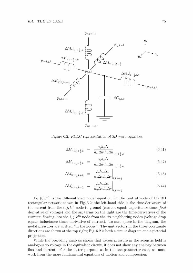
6.4. THE 3D CASE 75
pppppppppppppppppppppppppppppppppppppppppp
pppppppppppppppppppppppppppppppppppppppppp
XXXXXXXXXXXX
XXX
XXX
XXXz
6
t
∆Ci,j,k
∆Mu|i+ 12 ,j,k
∆Mu|i− 12 ,j,k
∆Mv|i,j− 12 ,k
∆Mv|i,j+ 12 ,k
∆Mw|i,j,k+ 12
∆Mw|i,j,k− 12
pi,j,k
pi,j,k+1
pi,j,k−1
pi,j−1,k
pi,j+1,k
pi−1,j,k
pi+1,j,k
ew
ev
eu
Figure 6.2: FDEC representation of 3D wave equation.
∆Mv|i,j+ 12 ,k =
ρohv∆vhw∆w hu∆u
∣
∣
∣
∣
∣
i,j+ 12 ,k
(6.41)
∆Mv|i,j− 12 ,k =
ρohv∆vhw∆w hu∆u
∣
∣
∣
∣
∣
i,j− 12 ,k
(6.42)
∆Mw|i,j,k+ 12
=ρohw∆w
hu∆uhv∆v
∣
∣
∣
∣
∣
i,j,k+ 12
(6.43)
∆Mw|i,j,k− 12
=ρohw∆w
hu∆uhv∆v
∣
∣
∣
∣
∣
i,j,k− 12
(6.44)
Eq. (6.37) is the differentiated nodal equation for the central node of the 3Drectangular network shown in Fig. 6.2; the left-hand side is the time-derivative ofthe current from the i, j, kth node to ground (current equals capacitance times firstderivative of voltage) and the six terms on the right are the time-derivatives of thecurrents flowing into the i, j, kth node from the six neighboring nodes (voltage dropequals inductance times derivative of current). To save space in the diagram, thenodal pressures are written “in the nodes”. The unit vectors in the three coordinatedirections are shown at the top right; Fig. 6.2 is both a circuit diagram and a pictorialprojection.
While the preceding analysis shows that excess pressure in the acoustic field isanalogous to voltage in the equivalent circuit, it does not show any analogy betweenflux and current. For the latter purpose, as in the one-parameter case, we mustwork from the more fundamental equations of motion and compression.

76 FINITE-DIFFERENCE EQUIVALENT-CIRCUIT (FDEC) MODEL
6.4.2 The equations of motion and compression
Recall that the linearized equation of motion in point form is
∇p = −ρoq (6.45)
(see Eq. (2.15)). For reasons which will become clear in Section 7.1, it is convenientto rewrite this equation in terms of phasors or Fourier transforms, obtaining
∇P = −jωρoQ. (6.46)
(Because the Fourier transform is defined for a wide range of functions, includingany function having a magnitude whose integral over the real line is finite, the lossof generality is not serious.)
If we introduce curvilinear orthogonal coordinates u, v, w, and take componentsin the u direction, Eq. (6.46) becomes
1hu
∂P∂u
= −jωρoQu (6.47)
which is the starting point for the finite-difference analysis.Let u, v, w take discrete values as defined in Section 6.2, and let the derivative
and other quantities in Eq. (6.47) be evaluated at (ui+ 12, vj, wk). Then the finite-
difference form of the equation is
1hu
∣
∣
∣
∣
i+ 12 ,j,k
Pi+1,j,k − Pi,j,k
∆u≈ −jωρo Qu|i+ 1
2 ,j,k , (6.48)
which may be written
Pi,j,k − Pi+1,j,k ≈ [jωρohu∆uQu]i+ 12 ,j,k . (6.49)
Now let us define “the unit cell centered on (ui+ 12, vj, wk)” as the quasi-cubic region
ui < u < ui+1 ; vj− 12
< v < vj+ 12
; wk− 12
< w < wk+ 12. (6.50)
The cross-sectional area of this unit cell at the surface u = ui+ 12
may be estimatedas
[hv∆v hw∆w]i+ 12 ,j,k .
To estimate the flux flowing through this cross-section in the direction of increasingu, we multiply the “area” by Qu|i+ 1
2 ,j,k. Hence the estimated flux is
∆Uu|i+ 12 ,j,k = [hv∆v hw∆w Qu]i+ 1
2 ,j,k . (6.51)
So, if we multiply and divide the right side of Eq. (6.49) by the estimated cross-sectional area and arrange the factors into appropriate groups, we obtain
Pi,j,k − Pi+1,j,k ≈ jω ∆Mu|i+ 12 ,j,k ∆Uu|i+ 1
2 ,j,k . (6.52)
where ∆Mu|i+ 12 ,j,k is defined in Eq. (6.39), above.
From the right-hand side of Eq. (6.39), we see that ∆Mu|i+ 12 ,j,k has the dimensions
of acoustic mass—the numerator is ρo times the estimated length of the unit cell

6.4. THE 3D CASE 77
-
t66 ∆Uu|i+ 1
2 ,j,k
∆Mu|i+ 12 ,j,k
Pi+1,j,kPi,j,k
Figure 6.3: FDEC representation of equation of motion in u direction, in free air.
centered on (ui+ 12, vj, wk), and the denominator is the estimated cross-sectional area
of the same unit cell. (Indeed, the definitions of the ∆C’s and ∆M ’s in equations(6.38) to (6.44) were guided by the desire to find subexpressions with the dimensionsof familiar quantities, and these dimensions were tacitly used in Fig. 6.2.) Hence onemay be tempted to conclude from Eq. (6.37) and Fig. 6.2 that the time-derivativeof the flux through the unit cell may be found by dividing the pressure differenceby the acoustic mass. Caution is required, however, because the velocity is notconstrained to lie in the direction of any one of the three coordinate unit vectors—the unit cell is not a horn or pipe. Moreover, the definition of acoustic mass makes a1P assumption (see the derivation of Eqs. (2.23) and (2.24)), whereas the derivationof Eq. (6.37) makes no such assumption. Eq. (6.52) has now settled the issue: if thepressures are evaluated at the midpoints of opposite faces of the unit cell, and if theflux is measured through the mid cross-section, then we have the usual relationshipbetween pressure, flux and acoustic mass.
Eq. (6.52) relates the pressure at the i, j, kth point to the pressure at one of thesix neighboring points in the 3D lattice. The pressure at the opposite neighbor-ing point is modeled by substituting i− 1 for i, yielding another equation similarto Eq. (6.52). Four more equations, incorporating the pressures at the other fourneighboring points, may be obtained by incrementing and decrementing j and k in-stead of i. Note that in the three equations in which the pressure at the neighboringpoint is indicated by decrementing a counter instead of incrementing it, the assumeddirection of the flux is towards the i, j, kth point instead of away from it.
Eq. (6.52) has the equivalent circuit shown in Fig. 6.3. Similar diagrams can bedrawn for the other five equations in the family; the positive direction of the fluxwill be towards the i, j, kth node in three cases, and away from it in the other threecases. When the six diagrams are combined, they give the six-way star connectionof acoustic masses shown in Fig. 6.2, with the same pressures (albeit in phasor form)and the same acoustic masses. Hence the fluxes must also be the same. It can beseen from the derivation of Eq. (6.51) that the flux in Fig. 6.3 is an estimate of theflux through one face of the init cell centered on (ui, vj, wk); hence all the fluxes inFig. 6.2 have that physical significance.
Further physical insights can be gained by finding an equivalent circuit for theequation of compression. Instead of using one of the existing forms of the equation,we shall revert to the equation of continuity, convert it to phasor form, then use apressure-density relation involving γ. This is not the most direct approach for theimmediate purpose of deriving an equivalent circuit, but will be useful for future

78 FINITE-DIFFERENCE EQUIVALENT-CIRCUIT (FDEC) MODEL
reference (Section 7.2).Recall that for small compressions, the point form of the equation of continuity
isρ = −ρo divq
(Eq. (2.30)). Let ρe be the excess density, i.e. the difference between the instanta-neous density ρ and the equilibrium or time-averaged density (not to be confusedwith ρo, which is a temporal and spatial average). As the equilibrium density istime-invariant, we have
ρ = ρe. (6.53)
Let the phasor representations of p and ρe be P and ρe, respectively. Writing ρe
for ρ in the equation of continuity and converting immediately to phasor form, weobtain
jωρe = −ρo divQ. (6.54)
Next we combine Eqs. (2.31) and (2.39) to obtain the pressure-density relation
dpdρ
=γP0
ρo. (6.55)
Multiplying both sides by ρ and using the chain rule on the left gives
p =γP0
ρoρ =
γP0
ρoρe (6.56)
which may be written in phasor form and divided through by jω to obtain
P =γP0
ρoρe. (6.57)
This is an alternative definition of γ (and will be used again in Section 7.2). Mul-tiplying both sides of Eq. (6.54) by γP0/ρo, then using Eq. (6.57) to rewrite theleft-hand side in terms of P , we obtain the equation of compression in phasor form:
jωP = −γP0 divQ. (6.58)
This is the starting point for the finite-difference treatment.In curvilinear orthogonal coordinates u, v, w, the divergence is given by [24,
p. 174]
divQ =1
huhvhw
[
∂∂u
(hvhwQu) +∂∂v
(hwhuQv) +∂
∂w(huhvQw)
]
. (6.59)
Now let us take discrete values of u, v, w as in the previous section. Then the i, j, kth
unit cell—that is, the unit cell centered on (ui, vj, wk)—has an estimated volume
∆V i,j,k = [hu∆u hv∆v hw∆w]i,j,k (6.60)
and hence the estimated compliance
∆Ci,j,k =∆V i,j,k
ρoc2 =∆V i,j,k
γP0=
[
hu∆uhv∆v hw∆wγP0
]
i,j,k
(6.61)

6.4. THE 3D CASE 79
(the second equality follows from Eq. (2.41)). So let us multiply the numerator anddenominator in Eq. (6.59) by ∆u∆v∆w, substitute for divQ in Eq. (6.58) and useEq. (6.61). This yields
jωPi,j,k = − 1∆Ci,j,k
∆u∆v∆w[
∂∂u
(hvhwQu) +∂∂v
(hwhuQv) +∂
∂w(huhvQw)
]
i,j,k
.
(6.62)Multiplying through by ∆Ci,j,k and replacing the partial derivatives by their finite-difference approximations, we obtain
jω∆Ci,j,k Pi,j,k ≈ −∆u∆v∆w
[hvhwQu]i+ 12 ,j,k − [hvhwQu]i− 1
2 ,j,k
∆u
+[hwhuQv]i,j+ 1
2 ,k − [hwhuQv]i,j− 12 ,k
∆v
+[huhvQw]i,j,k+ 1
2− [huhvQw]i,j,k− 1
2
∆w
. (6.63)
Now in the i, j, kth unit cell, the flux in the positive u direction through the faceu = ui+ 1
2is
∆Uu|i+ 12 ,j,k = [hv∆v hw∆w Qu]i+ 1
2 ,j,k (6.64)
(which agrees with Eq. (6.51)), and the flux in the same direction through the faceu = ui− 1
2is
∆Uu|i− 12 ,j,k = [hv∆v hw∆w Qu]i− 1
2 ,j,k . (6.65)
In an analogous manner we may define ∆Uv|i,j+ 12 ,k, ∆Uv|i,j− 1
2 ,k, ∆Uw|i,j,k+ 12
and∆Uw|i,j,k− 1
2. Expanding the right-hand side of Eq. (6.63) and renaming the subex-
pressions just defined, we obtain the desired result
jω∆Ci,j,k Pi,j,k ≈ ∆Uu|i− 12 ,j,k − ∆Uu|i+ 1
2 ,j,k
+ ∆Uv|i,j− 12 ,k − ∆Uv|i,j+ 1
2 ,k
+ ∆Uw|i,j,k− 12− ∆Uw|i,j,k+ 1
2. (6.66)
This equation describes the circuit shown in Fig. 6.4. To save space in the dia-gram, the pressure at the i, j, kth node is written “in the node”, while the branchfluxes are written in line with the branches. The unit vectors in the three coor-dinate directions are shown at the top right. Eq. (6.66) states that the compliantadmittance times the pressure is equal to the sum of fluxes into the compliantelement—or, in analogous electrical terms, that the capacitive admittance times thevoltage is equal to the sum of currents into the capacitive element.
The fluxes in Fig. 6.4 are the same as those in Fig. 6.3 and the other five equivalentcircuits from the equation of motion. The six circuits for the equation of motionalso include Pi,j,k. So Fig. 6.4 may be combined with the six inertance circuits toproduce the complete circuit of Fig. 6.2, with the flux information added.
Fig. 6.2 is the result of a “pure” finite-difference approximation to the waveequation. The derivations of Figs. 6.3 and 6.4 used “estimated” values of area, flux,volume and compliance, but these estimates were not used in deriving Fig. 6.2, which

80 FINITE-DIFFERENCE EQUIVALENT-CIRCUIT (FDEC) MODEL
6
6
XXXXXXXXz
XXXXXXXXXXXz
XXXz
6
t ew
ev
eu
∆Ci,j,k
∆Uu|i+ 12 ,j,k
∆Uu|i− 12 ,j,k
∆Uv|i,j+ 12 ,k
∆Uv|i,j− 12 ,k
∆Uw|i,j,k+ 12
∆Uw|i,j,k− 12
Pi,j,k
Figure 6.4: FDEC representation of 3D equation of compression, in free air.
includes all the information in Figs. 6.3 and 6.4 except the fluxes. Thus the fluxesare the only quantities in the equivalent circuits which involve approximations otherthan the basic finite-difference approximation. The flux approximation becomessignificant when the velocity at the boundary of a unit cell must be modeled as aflux through one face of the unit cell.
6.4.3 Truncated elements at boundary surfaces
Arai [2] did not consider boundary conditions in the 3D case; he did not need to,because all his computational examples were one-dimensional. In this thesis, 3Dboundary conditions will be considered only at equicoordinate boundaries. The useof curvilinear orthogonal coordinates allows a limited but useful variety of boundarysurfaces to be modeled as equicoordinate surfaces. More complex surface shapesmay be approximated by piecewise-equicoordinate surfaces.
As in the 1P case, the difficulty with boundary conditions is that the pressure andthe velocity are sampled at different points; the velocity sampling points for ∆Uu,∆Uv and ∆Uw are displaced from the pressure sampling points by ±∆u/2, ±∆v/2and ±∆w/2 in the u, v and w directions, respectively. The solution, modeled onSubsection 6.3.3, is to extend the definitions in Section 6.2 so as to allow i, j, k tobe multiples of one quarter, and take extra samples at the boundary. As far asthe equations describing a single element are concerned, there is nothing specialabout the “standard” increments ∆u, ∆v, ∆w; the increments are arbitrary and canbe changed at our convenience. The purpose of using uniformly spaced samplingpoints, referred to by subscripts, is to ensure that each sample of pressure or velocityis involved in the difference equations of several elements, so that the elements canbe connected into circuits. At the boundaries of the region under study, however,it is convenient to vary the spacing of sample points. The necessary variations areeasily expressed by modifying the subscripts.
The rules for evaluating the normal (interior, non-truncated) FDEC elementsare as follows:

6.4. THE 3D CASE 81
• In the formula for a component value, scale factors are evaluated at the body-center of the element (mass or compliance);
• In a circuit equation involving a mass element, pressure is sampled at thecenters of two opposite faces of the element, chosen so that the normals tothe two faces are in the direction of the velocity component governed by thatelement;
• In a circuit equation involving a compliance element, the areas of the six facesand the fluxes passing through them are calculated using the scale factors andvelocities sampled at the centers of the six faces of the element.
For the truncated elements, we simply apply the same rules using the new elementdimensions, using subscripts to indicate the coordinates of the new element sur-faces. In the above list, the word “center” refers to the midranges of the variablecoordinates—two coordinates for a face-center and three for a body-center. As inSubsection 6.3.3, if we wish to interpret the names of the elements as functions ofthe subscripts, the name of a truncated element will include a multiplier.
Suppose we wish to impose a boundary condition at the surface u = ui+ 12
whenthe pressure is sampled at an array of points on the surface u = ui. By rotatingcoordinates in Eq. (6.50)), it can be seen that the boundary surface passes betweentwo layers of inertia elements in the v direction, and between two layers of inertiaelements in the w direction, so that the inertia elements in those directions areunaffected. But Eq. (6.50), as written, indicates that the boundary surface cutsthrough a layer of inertia elements in the u direction. Accordingly, given an originalpressure sample Pi,j,k, we need to take an extra sample Pi+ 1
2 ,j,k. If the pressureis evaluated at (ui+ 1
2, vj, wk) instead of (ui+1, vj, wk), Eqs. (6.52) and (6.39) are
replaced byPi,j,k − Pi+ 1
2 ,j,k ≈ jω 12 ∆Mu|i+ 1
4 ,j,k ∆Uu|i+ 14 ,j,k (6.67)
where ∆Uu|i+ 14 ,j,k and ∆Mu|i+ 1
4 ,j,k are defined as in Eqs. (6.51) and (6.39), with i + 14
in place of i + 12 ; that is,
∆Uu|i+ 14 ,j,k = [hv∆v hw∆w Qu]i+ 1
4 ,j,k (6.68)
and12 ∆Mu|i+ 1
4 ,j,k =12
ρohu∆uhv∆v hw∆w
∣
∣
∣
∣
∣
i+ 14 ,j,k
=ρohu
12∆u
hv∆v hw∆w
∣
∣
∣
∣
∣
i+ 14 ,j,k
. (6.69)
Thus, between the original sample Pi,j,k and the extra sample Pi+ 12 ,j,k, there is an
acoustic mass with the usual cross sectional area and half the usual length, with the“area” and “length” estimated from the scale factors at the mean values of u, v, w.A similar conclusion follows if the desired extra sample is Pi− 1
2 ,j,k instead of Pi+ 12 ,j,k;
the relevant equations may be found by writing i− 12 for i in Eqs. (6.67) and (6.69).
Four more equations, expressing similar conclusions, may be written for the othertwo coordinate directions. In total, we have six ways to construct an equivalentcircuit incorporating an extra pressure sample. One of the six variations will beused in Chapter 11 to impose a far-field radiation condition in a simulation of apiston-radiator in an infinite planar baffle.

82 FINITE-DIFFERENCE EQUIVALENT-CIRCUIT (FDEC) MODEL
Recall that ∆Uu|i+ 14 ,j,k is a non-FDM estimate of the flux through the mean
surface (u = ui+ 14) of the shortened inertia element ∆Mu|i+ 1
4 ,j,k. Because this iner-tial element is lumped and is a terminal element in the network, ∆Uu|i+ 1
4 ,j,k alsoestimates the flux through the boundary surface element
u = ui ; vj− 12
< v < vj+ 12
; wk− 12
< w < wk+ 12. (6.70)
A second method of truncating a 3D equivalent circuit, which will be derivedbut not used in this thesis, is required if we wish to impose a boundary conditionat the surface u = ui when the velocity is sampled at an array of points on thesurface u = ui− 1
2. Given an original velocity sample Qu|i− 1
2 ,j,k, we must take anextra sample Qu|i,j,k. The boundary surface passes between two layers of inertiaelements in the u direction, so these elements are unaffected. But the boundarycuts through a layer of compliance elements, a layer of inertia elements in the vdirection, and a layer of inertia elements in the w direction, so these elements mustbe redefined as truncated elements. Thus the second method of truncation affectsthree sets of elements while the first method affects only one; that is why the firstmethod is preferred in Chapters 10 and 11.
The “half unit cell” defined by
ui− 12
< u < ui ; vj− 12
< v < vj+ 12
; wk− 12
< w < wk+ 12. (6.71)
has an estimated compliance of 12∆Ci− 1
4 ,j,k. The estimated flux in the positive udirection through the face u = ui is
∆Uu|i,j,k = [hv∆v hw∆w Qu]i,j,k (6.72)
and the estimated flux in the same direction through the face u = ui− 12
is
∆Uu|i− 12 ,j,k = [hv∆v hw∆w Qu]i− 1
2 ,j,k . (6.73)
In the above two equations, the quantity ∆Uu is defined, with its subscripts, as inEq. (6.51). In the next four equations, corresponding definitions will be used for∆Uv and ∆Uw. In the half unit cell defined by Eq. (6.71), the estimated flux in thepositive v direction through the face v = vj+ 1
2is
12 ∆Uv|i− 1
4 ,j+ 12 ,k =
[
hu12∆uhw∆w
]
i− 14 ,j+ 1
2 ,k(6.74)
and the estimated flux in the same direction through the face v = vj− 12
is
12 ∆Uv|i− 1
4 ,j− 12 ,k =
[
hu12∆uhw∆w
]
i− 14 ,j− 1
2 ,k. (6.75)
The estimated flux in the positive w direction through the face w = wk+ 12
is
12 ∆Uw|i− 1
4 ,j,k+ 12
=[
hu12∆uhv∆v
]
i− 14 ,j,k+ 1
2
(6.76)
and the estimated flux in the positive w direction through the face w = wk− 12
is
12 ∆Uw|i− 1
4 ,j,k− 12
=[
hu12∆uhv∆v
]
i− 14 ,j,k− 1
2
. (6.77)

6.5. 3D BOUNDARY CONDITIONS 83
With the new compliance and fluxes thus defined, Eq. (6.66) is replaced by
jω 12∆Ci− 1
4 ,j,k Pi− 14 ,j,k ≈ ∆Uu|i− 1
2 ,j,k − ∆Uu|i,j,k+ 1
2 ∆Uv|i− 14 ,j− 1
2 ,k −12 ∆Uv|i− 1
4 ,j+ 12 ,k
+ 12 ∆Uw|i− 1
4 ,j,k− 12− 1
2 ∆Uw|i− 14 ,j,k+ 1
2. (6.78)
This equation has the same form as Eq. (6.66) and describes a circuit of theform shown in Fig. 6.4, but with different component values and fluxes to reflect thedifferent location and dimensions of the volume element.
Considering the fluxes in Eq. (6.78), we may observe that ∆Uu|i− 12 ,j,k is just
the estimated flux in the internal mass element ∆Mu|i− 12 ,j,k (cf. Eq. (6.52)), and is
therefore already represented in the equivalent circuit. ∆Uu|i,j,k is the estimatedflux through the boundary surface element given by Eq. (6.70). The remaining fourfluxes flow in the truncated mass elements which are left after the boundary surfacehas cut through a layer of original mass elements in the v and w directions. Forexample, an equation of motion involving 1
2 ∆Uv|i− 14 ,j− 1
2 ,k may be constructed bymodifying the subscripts in Eqs. (6.52) and (6.39):
Pi− 14 ,j−1,k − Pi− 1
4 ,j,k ≈ jω 2∆Mv|i− 14 ,j− 1
2 ,k12 ∆Uv|i− 1
4 ,j− 12 ,k (6.79)
where
2∆Mv|i− 14 ,j− 1
2 ,k =ρohv∆v
hu12∆uhw∆w
∣
∣
∣
∣
∣
i− 14 ,j− 1
2 ,k
. (6.80)
The reason for the factors 2 and 12 in the above two equations is that the symbols ∆Mv
and ∆Uv are defined for unit cells of standard dimensions; see Eqs. (6.39) to (6.44)and Eq. (6.51). The multiplying factor in front of the inertance not only preservesnotational consistency, but also indicate how the changes in cell dimensions affectthe boundary inertances, and hence how the boundary inertances compare withadjacent interior inertances.
Another three pairs of equations may be written for the other fluxes in Eq. (6.78),and another five equations similar to Eq. (6.78) may be written for the other fiveways in which one might impose a boundary at an array of pressure sampling points,requiring additional velocity samples.
6.5 3D boundary conditions
The discussion of 1P boundary conditions in Subsection 6.3.3 concerned the problemof truncating the L-C ladder network at a single point when pressure and flux weresampled at different points. The solution was to use the finite-difference approxima-tion with a reduced step size to take an additional sample. Once the network wassuccessfully truncated at the boundary, the problem of applying the actual bound-ary condition—source or impedance—was trivial, and did not need to be discussedat length.
Subsection 6.4.3 is modeled on Subsection 6.3.3 and therefore also concerns it-self with truncating the network at the given boundary, and not with applying theactual boundary condition. But in the 3D case, the application of the boundary con-dition involving velocity or admittance is no longer trivial, for two reasons. First,

84 FINITE-DIFFERENCE EQUIVALENT-CIRCUIT (FDEC) MODEL
the boundary condition applies to a distributed quantity, whereas the equivalentcircuit comprises lumped components. Second, a velocity or admittance has a direc-tion, which is not necessarily normal to the boundary. The procedure for modelinga 3D boundary condition will usually involve replacing a velocity with a lumpedflux, and this step (as noted at the end of Subsection 6.4.2) requires a non-FDMapproximation.
6.5.1 Pressure condition
The imposition of a pressure at a boundary is easily modeled. Because p is ascalar, the orientation of the boundary is not involved in the specification of theboundary condition. Moreover, p is directly represented in the equivalent circuit;the finite step size requires that p be sampled, but does not require conversion toa lumped quantity, e.g. a force. Thus it suffices to terminate the equivalent circuitwith pressure sources at the appropriate nodes.
The pressure condition is the only 3D boundary condition that does not requirea non-FDM approximation.
6.5.2 Normal velocity condition
A smooth vibrating surface in contact with a fluid determines the fluid velocity nor-mal to the surface. Because the surface is moving, it imposes its normal velocityat a point moving with the fluid, whereas the linearized equations of motion andcompression, on which the FDEC model is based, involve the fluid velocity at sta-tionary points. Thus it is necessary to distinguish between the physical boundary,which moves, and the model boundary, which is stationary at the mean position ofthe physical boundary. For small oscillations, the fluid velocity at any point on thephysical boundary will be nearly equal to the fluid velocity at the mean positionof that point, so that we may consider the boundary condition to be imposed atthe model boundary rather than the physical boundary. This approximation is thetime integral of the corresponding approximation in Subsection 2.1.2, on which thelinearization of the equation of motion is based; if we neglect the quadratic termsin Eq. (2.8), we see that the acceleration of a point moving with the fluid (the totalderivative of velocity) can be approximated by the derivative of the velocity at afixed point (the partial derivative of velocity).
Let qn be the imposed normal velocity, n the unit normal vector to the modelboundary (in the agreed positive direction of qn), and q the fluid velocity. Then theboundary condition is simply
q.n = qn (6.81)
or, in phasor form,Q.n = Qn. (6.82)
Now suppose the model boundary is a constant-u surface, so that the area elementof the surface is approximately hv∆v hw∆w. If we multiply both sides of Eq. (6.82)by this area, the left-hand side becomes an estimate of the (phasor) flux through thearea element. Denoting this flux by ∆U , we may rewrite the boundary condition as
∆U = hv∆v hw∆w Qn. (6.83)

6.5. 3D BOUNDARY CONDITIONS 85
As usual, the scale factors and Qn should be evaluated at the middle values of v andw for each surface element. Surfaces of constant v or w are treated similarly. Thusa normal velocity condition is modeled by terminating the network with an array offlux sources.
6.5.3 Normal admittance condition
Let P denote the phasor pressure. As in Subsection 3.3.4, let us define the specificacoustic admittance at a point in the acoustic field as the complex vector
y =QP
. (6.84)
Let us also define the normal specific acoustic admittance at a point on the boundaryas the complex scalar
yn =Qn
P. (6.85)
Using these two notations, we may divide Eq. (6.82) through by P and obtain
y.n = yn (6.86)
which shows that yn is the normal component of y.3
Now let us define the acoustic admittance of the boundary element as the complexscalar
∆Y =∆UP
. (6.90)
Dividing Eq. (6.83) by P and using the notations of Eqs. (6.85) and (6.90) gives
∆Y = hv∆v hw∆w yn. (6.91)
In words, this result says that the acoustic admittance is approximately equal tothe normal specific acoustic admittance multiplied by the area element; “specific”means “per unit area” (the same conclusion was made concerning the radial specificacoustic admittance in Subsection 3.3.4). Thus a normal admittance condition ismodeled by terminating the network with an array of lumped admittances.
3There is no corresponding result concerning impedances. The reciprocal of the vector y is notdefined, so there is no obvious way to define a vector impedance. We can obtain a scalar impedanceby defining the normal specific acoustic impedance as
zn = 1/yn. (6.87)
But, if the angle between y and n is α, Eq. (6.86) can be written
yn = |y| cos α. (6.88)
Taking reciprocals gives the normal specific acoustic impedance
zn =1|y|
secα (6.89)
which is clearly not the normal component of a vector.

86 FINITE-DIFFERENCE EQUIVALENT-CIRCUIT (FDEC) MODEL
6.5.4 Anechoic or free-air radiation condition
For engineering purposes it is convenient to describe an acoustic radiator in termsof its free-air radiation pattern, i.e. its radiation into an infinite three-dimensionalexpanse of air (cf. the free-space radiation pattern of a radio antenna). Because noinfinite expanse of air exists, practical measurements of free-air radiation charac-teristics are often performed in an anechoic chamber, whose walls are designed toabsorb sound waves just as they would be “absorbed” by an imaginary surface infree air. Calculation of free-air radiation by the FDEC method presents a similarproblem with a similar solution: because the modeling of an infinite volume of airwith a finite step size would require an infinite amount of computation, one mustmodel a finite volume and simulate the interface between the finite and infinitevolumes by imposing an appropriate boundary condition.
A thin, impermeable membrane suspended in a fluid will not interfere with thepropagation of sound through the fluid if the membrane moves exactly as the fluidwould move in the absence of the membrane. If the fluid is inviscid, it is sufficientthat the normal velocity of the membrane match the normal velocity of the fluid inthe absence of the membrane (here “normal” means “normal to the membrane”).Hence, if the pressure distribution on one side of the membrane is given, it is suffi-cient that the ratio of the normal velocity phasor to the pressure phasor be the sameas if the membrane were absent; this ratio is the above-mentioned normal specificacoustic admittance, denoted by yn. So, as far as the acoustic field on one side of themembrane is concerned, the membrane will be indistinguishable from a continuationof the fluid if it imposes the same yn.
Therefore, to model the acoustic field radiated by a distributed source in free airusing the FDEC method, we choose an equicoordinate (or piecewise-equicoordinate)surface enclosing the source, construct the FDEC model of the enclosed volume,and terminate the network so as to represent the normal admittance condition asdescribed above (Subsection 6.5.3).
The difficulty with this procedure is that the representation of the normal ad-mittance condition depends on the specific acoustic admittance y, which in turndepends on the radiated acoustic field—i.e. on the unknown quantity that we aretrying to determine. However, if the dimensions of a distributed acoustic sourceare much smaller than the shortest distance from the source to the boundary of thesimulated region, we might expect to be able to estimate y at every point on theboundary by replacing the distributed source with a point-source. The apparentstrength of the point source may vary with angular position (due to diffraction andinterference), but the admittance should not be affected. This intuitive expectationis supported by the following argument.
Suppose a distributed acoustic source, of finite size and with sinusoidal timedependence, is placed near the center of a spherical coordinate system (R, θ, φ)in free air. Let U0 be the total flux produced by the source (integrated over theradiating surface). If U0 is non-zero, the pressure phasor at a general point may bewritten in the form
P = D(ω, r, θ, φ) U0jωρo
4πe−jkr
r(6.92)
where k = ω/c, as usual. Because D(ω, r, θ, φ) is a perfectly general function, andbecause the other factors on the right are non-zero, we can always find D to satisfy

6.5. 3D BOUNDARY CONDITIONS 87
Eq. (6.92). The form of this equation has been chosen because it is equivalent to
P = D(ω, r, θ, φ) PPS(ω, r) (6.93)
where PPS(ω, r) is the pressure due to a point-source at the origin producing thesame total flux as the distributed source (cf. Eq. (3.22)). Thus D is introduced bythe spatial distribution of the source and may be called a distribution factor.
Let us define a “wavefront” as a surface over which the phase of P is constant.For large r, the source subtends a small angle, so that we can speak of a “line of sightto the source”, to which the wavefronts are perpendicular; hence the wavefronts canbe approximated by r-surfaces, i.e. by spheres centered on the origin. Now considera narrow cone with its apex at the origin. Because the cone is narrow, there isnegligible variation of |P | with θ and φ within the cone, so that the r-surfaceswithin the cone are surfaces of nearly constant P . Moreover, the cone is a tube oforthogonal trajectories to the r-surfaces, and r has a scale factor of unity. ThereforeWebster’s equation in the coordinate r is an approximate model of the field withinthe cone. The most general solution to the time-independent Webster equation inr, subject to the restriction that there is only an outward-traveling wave, can bewritten in the form
P = D(ω) PPS(ω, r) (6.94)
(cf. Eqs. (3.17) and (3.22)). Note that D(ω) has no r-dependence. Widening thecone to include all of 3D space may cause D to depend on θ and φ, but it cannotmake D depend on r as in Eq. (6.93), because the r-dependence is in the factor PPS.So for sufficiently large r, we can neglect the r-dependence of D in Eq. (6.93) andobtain
P D(ω, θ, φ) PPS(ω, r). (6.95)
If we think of D as modifying the U0 factor in PPS, the above expression lookslike the pressure due to a point-source whose apparent strength varies with angularposition.
To find an expression for the velocity, we first use Eq. (6.93) in the equation ofmotion:
Q = − 1jωρo
∇P = − 1jωρo
∇(DPPS)
= − 1jωρo
(D∇PPS + PPS∇D)
= D(
− 1jωρo
∇PPS
)
− PPS
jωρo∇D. (6.96)
The expression in parentheses may be recognized as QPS, the velocity accompanyingthe point-source pressure field PPS. Hence, if we divide Eq. (6.96) by Eq. (6.95), weobtain
QP
=QPS
PPS− 1
jωρo
∇DD
. (6.97)
The left-hand side is the specific acoustic admittance y. The first term on the right isthe point-source specific acoustic admittance, which we may call yPS. The gradientof D, in spherical coordinates with negligible r-dependence, is
∇D 1r
∂D∂θ
eθ +1
r sin θ∂D∂φ
eφ (6.98)

88 FINITE-DIFFERENCE EQUIVALENT-CIRCUIT (FDEC) MODEL
(it is here that we first exploit the form of D in Eq. (6.95)). Making these substitu-tions in Eq. (6.97), we obtain
y yPS −1
jωρoD
(
1r
∂D∂θ
eθ +1
r sin θ∂D∂φ
eφ
)
. (6.99)
If D is nearly independent of r, so are its derivatives w.r.t. θ and φ. So as r increases,both terms in parentheses approach zero and the entire right-hand side approachesyPS. That is, the specific acoustic admittance in the far field can be estimated byassuming a point-source.
The derivation of this result assumes the existence of a function D to satisfyEq. (6.92), which in turn requires that U0, the total flux radiated by the source,is non-zero. Thus the far-field point-source approximation is not valid for a dipolesource or for an oscillating rigid body whose volume remains constant. In particular,it is not valid for an unbaffled rigid disk oscillating along its axis; an example of theerror caused by the point-source assumption in this case is given in Chapter 11.
While the assumption that U0 6= 0 is essential to the above argument, the free-airassumption can be widened in the manner of Subsection 3.3.2. A source near a rigidplanar baffle can be handled by the image method: the source and its image aretreated as a single source in free space, so the conclusion that y yPS holds in thefar field of the composite source. This result is used in Chapter 11 in the modelingof a circular rigid piston in an infinite planar baffle.
The same result can be extended, albeit with some loss of rigor, to the case of asource in the throat of an infinite “asymptotically conical horn”, i.e. a horn which isapproximately (or exactly) conical at large distances from the throat. Q and y arealmost purely radial in the far field of a source in free air. Hence, if we introducean asymptotically conical horn with the apex of its “asymptotic cone” at the origin,the far field will not be greatly disturbed, while the part of the horn in the near fieldcan be considered part of the source. In free air, the specific acoustic impedancein the far field of this composite source is approximately the same as that due to apoint-source, and is not greatly altered by adding the far-field portion of the horn.
6.5.5 Non-equicoordinate boundaries
Any boundary surface can be approximated by a piecewise-equicoordinate surface,and the approximation can be made arbitrarily accurate by taking a sufficiently smallstep size. However, unless the given surface is exactly equicoordinate, the piecewise-equicoordinate approximation cannot be made smooth but must be assembled fromquasi-cubic “blocks”. This non-smoothness does not prevent the approximation frombeing arbitrarily accurate in the sense that every point on the piece-wise equicoordi-nate surface can be made arbitrarily close to the desired surface. But it complicatesthe application of some boundary conditions.
For the pressure condition, the error in approximating the boundary surface be-comes an error in the location of each imposed pressure. The well-known Rayleighcriterion indicates that the resulting error in the simulation will not be objection-able provided that the boundary is approximated to within a small fraction of awavelength.
A normal-velocity (or normal-admittance) condition can be applied to eachequicoordinate segment by multiplying the original normal velocity (or normal ad-mittance) by the cosine of the angle between the equicoordinate segment and the

6.6. REDUCTION TO TWO DIMENSIONS 89
original surface. This cosine is of course a direction cosine of the normal to theoriginal surface. The procedure works because the normal velocity then makes thesame flux in the equicoordinate segment as it makes in the normal projection of thesegment on the original surface, and because these projections are contiguous on theoriginal surface.
A radiation condition is not affected at all, because there is no “given” surfaceto be approximated. The boundary of the model is arbitrarily chosen, and the radi-ation condition is expressed as a normal admittance condition by taking the normalcomponent of the vector specific acoustic admittance y. This procedure is conve-nient in the case of a piecewise-equicoordinate boundary because the component ofy normal to each boundary segment is the component in the direction of one of thethree coordinates. But in principle a piecewise-equicoordinate boundary is treatedlike any other.
In summary, only the normal-velocity and normal-admittance conditions requirespecial treatment when a given boundary is replaced by a piecewise-equicoordinateapproximation.
6.6 Reduction to two dimensions
We have seen in Section 6.3 that if P is a function of a single spatial coordinate, theFDEC model reduces to a ladder network. The present section shows that if P is afunction of two coordinates, say u and v, then the FDEC model can be reduced toa two-dimensional network.
If P is independent of the coordinate w, any finite-difference estimate of ∂P∂w will
produce the correct result, namely zero, regardless of the step size. In Eq. (6.35), theinner derivative w.r.t. w will be correctly estimated as zero; hence the parenthesizedexpression containing ∂p
∂w will evaluate to zero, and its derivative w.r.t. w will alsobe correctly estimated as zero. So, when deriving the FDEC model from the waveequation, we can use any step size ∆w without incurring any error. In the equationof motion in the w direction, which can be obtained by writing w for u in Eq. (6.47),the derivative w.r.t. w will be estimated as zero for all ∆w. The same equationof motion gives Qw = 0. Hence the derivative w.r.t. w in Eq. (6.62), which is anintermediate form of the equation of compression, will also be estimated as zero forall ∆w. In summary, in all the equations from which we can derive the FDEC model,the finite-difference approximations to the derivatives w.r.t. w are exact for all ∆wif P is independent of w.
The problem of finding necessary and sufficient conditions under which a coor-dinate system admits two-parameter waves, unlike the corresponding problem forone-parameter waves, is not considered in this thesis. In practice, however, we donot argue that “by symmetry, P is independent of w,” unless all three scale factorsand all three components of Q are also independent of w; if these conditions are notmet, there will be no prima facie appearance of “symmetry”.4 If the scale factorsand velocity components are independent of w, then the accuracy of the estimates
4Of course the w-independence of the components of Q can be deduced from the w independenceof P and the scale factors, using the equation of motion. But if we assert “By symmetry. . . ”, wewill consider all these facts to be self-evident. This argument applies when the wave functiondepends on exactly two coordinates; if it depends on only one coordinate, the scale factors for theother two coordinates must behave according to Eq. (5.7).
90 FINITE-DIFFERENCE EQUIVALENT-CIRCUIT (FDEC) MODEL
of areas and fluxes is not affected by the range of w (see e.g. Eq. (6.51)), so that noloss of accuracy is incurred by using a large ∆w.
Similarly, the “by symmetry” argument will not be possible unless the range of(u, v) for the simulated region is independent of w or—which is the same thing—therange of w is independent of u and v.
So, if the range of w for the whole system is a < w < b, we might as well choose∆w = b− a and let the compliance elements extend over the entire range of w. Asthere is no component of Q in the w direction, the truncated inertance elementsin the w direction will carry no flux and can be ignored. Thus the FDEC networkis only one element thick in the w direction; that is, it is two-dimensional. Thistechnique will be used to advantage in Chapters (10) and (11). The two-parameterassumption will approximate in Chapter 10, but exact in Chapter 11.

Chapter 7
The damped FDEC model (forfiber-filled regions)
For the purpose of damping unwanted internal resonances, loudspeaker boxes areoften filled with loose fiberglass or other low-density fibrous materials. Arai notes inpassing that the viscous losses and thermal absorption losses of such materials maybe modeled by using complex values of density and bulk modulus [2, p. 17]. But hegives no formulae, cites no references, and does not indicate how the results may beexpressed as modified circuits.
This chapter shows that the presence of fiber gives two main mechanisms ofdamping: direct viscous damping of the air motion, and conduction of the heat ofcompression between the air and the fiber. The viscous effect can be representedby introducing a complex value of density into the phasor form of the differentialequation of motion. In the equivalent circuit, this causes a parallel R-L circuit toappear in series with each ∆M . The thermal effect can be accounted for by usinga complex value of γ in the phasor form of the differential equation of compression.In the equivalent circuit, this causes a series R-C circuit to appear in parallel witheach ∆C. The complex bulk modulus (referred to by Arai) can be written in termsof the complex gamma.
In the terminology of this Chapter and Chapter 10, the word “fiber” (in thesingular) usually denotes the loosely-packed damping material as a whole, or a smallvolume element thereof; a single strand is referred to as a “filament”. In contrast,“fibers” (plural) always means a plurality of filaments, not a plurality of volumeelements or materials. Although contradictory, this usage is convenient and thecontext prevents any confusion. (In Chapter 8, which contains a long mathematicalanalysis of the conduction of heat to and from “one fiber”, it is more convenient touse the singular “fiber” in the discrete sense, consistent with the plural.)
7.1 Equation of motion: complex density
In free air, i.e. without damping material, Eq. (6.46) gives a relation between pressureand velocity in phasor form. We might expect the presence of the damping materialto alter this relation in a frequency-dependent manner, so that the new relationcould be described simply by replacing the density ρo with a frequency-dependentcomplex quantity ρ?; that is
∇P = −jωρ?Q. (7.1)
91

92 DAMPED FDEC MODEL (FIBER-FILLED REGIONS)
We shall see that the equation of motion of air in the presence of fiber can indeed bewritten in this form, and leads to an intuitively plausible modification to the inertiaelements of the finite-difference equivalent circuit.
7.1.1 Discussion of approximations; review of literature
A quantity called complex density was derived and used by Leach in his 1989 paperon fiber-filled enclosures [30]. Leach’s application is simpler than the present one inthat it does not involve the finite-difference method; the complex density expressionis substituted into a conventional low-frequency model of an undamped enclosure.But Leach’s expression for complex density is more complicated than the one to bederived here. His equation (21), which describes the motion of the fiber, includesthree force terms, namely
(a) a damping force proportional to the relative velocity between thefiber and the air,
(b) a second damping force proportional to the “absolute” velocity ofthe fiber, and
(c) an elastic restoring force proportional to the displacement of the fiberfrom the equilibrium position.
Leach’s analysis assumes that forces (b) and (c) are uncoupled, i.e. independent ofthe motion of adjacent fibers or even adjacent parts of the same filament. Thisis unrealistic given that both forces are internal to the fiber and arise from non-uniformity in the motion of the fiber (which causes deformation) rather than themotion itself. In Leach’s defense, it should be noted that the distinction betweenmotion and deformation is not critical in his analysis because the two quantities maybe assumed to be proportional; the entire volume of the fiber-filled box is modeled asa single volume element, with the fiber constrained to be stationary at the boundary.But in the general finite-difference volume element, no such constraint applies, sothat deformation and displacement must not be confused.
If deformation and displacement are proportional, as Leach may have assumed,then velocity is proportional to strain rate, which in turn may be proportional tointernal viscous forces. But one would not expect such forces to be significant whencompared with elastic forces, especially in a brittle material such as glass. Moreover,frictional forces caused by fibers sliding over adjacent fibers are not proportional tovelocity—absolute or relative. Hence one must question Leach’s treatment of force(b) even for his own purposes.
One may be tempted to neglect forces (b) and (c) solely because of lack of realism.But it is preferable to show that these forces are negligible compared with (a), theair drag. The following argument proceeds in two steps, suggesting that (b) is lesssignificant than (c), which in turn is negligible compared with (a).
Force (b) comprises viscous forces within each filament, plus friction due tofibers sliding over fibers. The internal viscous forces are expected to be smallerthan elastic forces, as already stated. Concerning friction, the fibers are excitedby a common airflow and therefore tend to move together with minimal sliding.If sliding is neglected, the only kind of frictional force is static friction, which isnon-dissipative and serves only to transmit the elastic force (c) through the fibernetwork.

7.1. EQUATION OF MOTION: COMPLEX DENSITY 93
To show that elastic forces (c) are negligible compared with air drag (a), onemay begin with a crude appeal to experience: anyone who has slept on an airmattress knows that the pillow section should not be fully inflated, or it will makean exceptionally hard “pillow”. But even a conventional soft pillow contains stuffingwhich is denser and harder than typical loudspeaker filling. This means that thebulk modulus of elasticity of the loosely packed fiber is much less than that of air,i.e. much less than ρoc2 (see Subsection 2.2.4). Assuming that the deformation ofthe fiber network is comparable with that of the air, the restoring forces within thefiber are small compared with those within the air, which in turn are comparablewith the air drag (a) if damping is significant. Hence the restoring forces (c) in thefiber are small compared with the air drag (a).
In a loudspeaker box, only the air motion contributes to radiation from a di-aphragm or vent. The fiber motion is of interest only insofar as it affects the airmotion. Now the internal forces in the fiber do not act directly on the air; theymust first accelerate the fiber, whose average density (mass per unit overall volume)is typically several times that of the air [30, p. 592]. We have established that therestoring forces in the fiber are small compared with the air drag provided that thebulk modulus of elasticity of the fiber network is much less than ρoc2. But becauseinternal forces in the fiber act on the fiber rather than the air, we can now weakenthis condition by replacing ρo with the average density of the fiber network, andstill be able to neglect the stiffness of the fiber for the purpose of calculating the airmotion. Let f be the filling factor, i.e. the fraction of the volume taken up by thefiber.1 Let the density of the glass (or other material of which the fiber is made)be ρf ; this is the intrinsic density, or the mass per unit volume of glass. Then theaverage density of the fiber network is fρf . Writing this density in place of ρo, wefind that we can neglect restoring forces in the fiber if the bulk modulus of the fibernetwork is much less than fρfc2. This conclusion is expressed in different notationby Bradbury, in a footnote to his 1976 paper [13]. Bradbury does not explain whythis condition is sufficient for the neglect of fiber stiffness, but indicates that thecondition always holds in practice “even for densely packed fibers”. The inflatable-pillow analogy, which leads to a stronger condition, makes his assurance easy tobelieve.
So Bradbury’s analysis deliberately neglects the elastic restoring forces in thefiber. It also neglects internal damping forces (not even mentioning them), leavingair drag as the only force in the equation of motion for the fiber. Hence Bradbury’sassumptions agree with those to be used here. His purpose, however, was quitedifferent; he did not use equivalent circuits or define a complex density, but wasinterested in the propagation velocities, attenuation rates and impedances of fiber-filled pipes.
One force not mentioned by Bradbury or Leach is gravity. Here it will be assumedthat the weight of the fibers is balanced by the quiescent internal forces in the fibers.But because of the low bulk modulus of the fiber network, the variations in theinternal forces will be assumed negligible compared with the air drag, as explainedabove. So gravity and the internal forces will be assumed to cancel out, and neitherwill appear in the equation of motion for the fiber.
1In Chapters 7, 8 and 10, the symbol “f” denotes the filling factor; frequency is specified interms of the angular frequency ω.

94 DAMPED FDEC MODEL (FIBER-FILLED REGIONS)
7.1.2 Derivation of complex density
To find an expression for complex density, we derive the equations of motion for theair and the fiber, then eliminate the fiber velocity between the two equations, ex-pressing the result in the form of Eq. (7.1). The elimination step is facilitated by writ-ing the equations of motion in terms of phasors or Fourier transforms, thereby con-verting the original differential equations into algebraic equations; it is a straightfor-ward example of solving simultaneous differential equations by a transform method.(Leach [30, p. 590] uses Laplace transforms instead of phasors.)
The difficult part is obtaining the two equations of motion. In keeping with thestandard established in Chapter 2, these equations will be derived more rigorouslythan in the papers of Leach and Bradbury. In particular, ρ and f will not be assumedconstant from the beginning, and when it does become necessary to assume themconstant, the approximation will be justified.
Let us suppose that the equilibrium values of all parameters of the fiber, includingthe filling factor f , are uniform throughout the filled region.2 The volume fractionoccupied by air is obviously 1− f . This is also the area fraction occupied by air inany cross-section through the filled region. Let q be the velocity of the air and qf
the velocity of the fibers. Let λ be the acoustic (or pneumatic) resistivity of the fiberfill; for present purposes this will be defined as the viscous force per unit velocityper unit volume of air,3 so that the viscous force per unit overall volume will be
(1− f)λ(q− qf)
on the fiber, with an equal and opposite force on the air. Note that λ is assumed tobe isotropic. This will be true if the orientation of fibers is completely random, butwill not if the fibers tend to run in a preferred direction or parallel to a preferredplane.
Now consider a three-dimensional region V enclosed by a surface σ moving withthe air. Newton’s second law for the air in this region is
ddt
∫∫∫
V(1− f) ρq dV = −
∫∫
σ(1− f) p .n dσ −
∫∫∫
V(1− f)λ(q− qf) dV (7.2)
where the integral on the left is the total momentum, and the integrals on the right(with the minus signs) are the hydrostatic and viscous forces.4 Using the gradient
2Here we apply the differential form of the equation of motion to a discontinuous medium—suchliberties are common in applied mathematics, as all media other than the perfect vacuum are madeof subatomic particles and are therefore discontinuous. In general, the use of a differential equationin a discontinuous medium requires that the particle spacing is small compared with the step sizeof a good finite-difference approximation to the differential equation. In the present case, the fiberradii and spacings must be small compared with the step size. The filling factor f is a statisticwhich depends on the volume sample chosen, but which is assumed to approach some limit as thesample size increases; the assumption that f is uniform means that the limit is independent of thesample location. We assume that the value of f is close to its limit for volume samples of a sizecomparable to that of a unit cell in the finite-difference network. In the text, the symbol f refersto this limiting value.
3Bradbury [13, p. 163] apparently defines λ with respect to overall volume, so that the factor(1− f) does not appear in his equation (1).
4In the original derivation of the point form of the equation of motion (Subsection 2.1.2), itwas shown that gravity and the gravitational pressure gradient may be neglected provided that weuse the pressure rise above equilibrium instead of the total pressure. This result is now assumedto hold in the presence of damping material. (A more rigorous approach would be to reworkSubsection 2.1.2 with the extra viscous force term.)

7.1. EQUATION OF MOTION: COMPLEX DENSITY 95
theorem to replace the surface integral with a volume integral, we obtain
ddt
∫∫∫
V(1− f) ρq dV = −
∫∫∫
V∇[(1− f)p] dV −
∫∫∫
V(1− f)λ(q− qf) dV . (7.3)
For small compressions, the fractional changes in f are small compared with thosein p; remember that p is the alternating excess pressure, not the total pressure.Moreover, because f is less than 0.01 for typical filling material5, the fractionalvariations in (1− f) are small compared with those in f . Thus the variations in(1− f) make negligible contribution to ∇[(1− f)p], so that (1− f) may be treatedas a constant and taken outside the ∇ operator. When this is done, the volumeintegrals can be rewritten in terms of the air mass element
dm = (1− f)ρdV (7.4)
so that the equation of motion becomes
ddt
∫∫∫
Vq dm = −
∫∫∫
V
∇pρ
dm−∫∫∫
V
λ(q− qf)ρ
dm. (7.5)
Note how the factor (1− f) has canceled out; this is one advantage of definingthe acoustic resistivity λ in terms of air volume rather than overall volume. Letus take the integrals over a single volume element, divide through by dm (as inSubsection 2.1.2), and make the small-amplitude approximation
dqdt
= q (7.6)
where the dot denotes partial differentiation (cf. Subsection 2.1.2 and especiallyEq. (2.8)). This gives
q = − 1ρ
[∇p + λ(q− qf)] . (7.7)
For small compressions we may replace ρ with ρo. Then we may convert to phasorform (assuming that λ is constant) and solve for ∇P , obtaining
∇P = λ(Qf −Q)− jωρoQ (7.8)
which is the desired form of the equation of motion for the air.6
Before shifting attention to the fiber, it is of interest to find another definitionof λ. If the motion of the air is steady and the fiber is stationary, we may put q = 0and qf = 0 in Eq. (7.7), and obtain
λq = −∇p. (7.9)
If electrical resistivity is represented (for the moment) by ρ, current density by Jand potential by V , the definition of resistivity is
ρJ = −∇V. (7.10)
5The “typical” figures given by Leach [30, p. 592] imply a filling factor of about 0.0025.6Eq. (7.8) agrees with Bradbury’s equation (11) in spite of his different definition of λ. However,
Bradbury also made it clear that he was not concerned about the small volume fraction occupiedby the fibers [13, pp. 163, 169].

96 DAMPED FDEC MODEL (FIBER-FILLED REGIONS)
Thus the chosen definition of pneumatic resistivity makes it analogous to electricalresistivity if we take q, rather than (1− f)q, as the analog of J.
Eq. (7.8) describes the motion of the air but involves the fiber velocity Qf , whichis usually not of interest except as regards its effect on the air motion. Anotherphasor equation will now be obtained from the equation of motion of the fiber, andwill be used to eliminate Qf . Consider a new control volume V enclosed by a newsurface σ, this time moving with the fiber. Remembering that the average densityof the fiber matrix (w.r.t. overall volume) is fρf , Newton’s second law for the fiberin this control volume may be written
ddt
∫∫∫
Vfρfqf dV =
∫∫∫
V(1− f)λ(q− qf) dV (7.11)
where the integral on the left is the total momentum of the fiber in the region, andthe integral on the right is the viscous force on the fiber. Both integrals can berewritten in terms of the fiber mass element
dmf = fρfdV . (7.12)
Then if we take the integrals over a single mass element, cancel dmf and use Eq. (7.6)for small oscillations, we obtain
fρf qf = (1− f)λ(q− qf) (7.13)
or, transposing all terms in qf to the left,
(1− f)λqf + fρf qf = (1− f)λq. (7.14)
Because the velocities are alternating while f and λ are mostly “DC”, we can treatf and λ as constants to obtain the phasor form
[(1− f)λ + jωfρf ] Qf = (1− f)λQ. (7.15)
Solving this for Qf and subtracting Q from both sides, using a common denominatoron the right, yields
Qf −Q = − jωfρf
(1− f)λ + jωfρfQ. (7.16)
To eliminate Qf , we substitute Eq. (7.16) into Eq. (7.8), obtaining the desiredform
∇P = −jωρ?Q (7.17)
wherejωρ? =
λ jωfρf
(1− f)λ + jωfρf+ jωρo. (7.18)
For the purpose of simplifying this expression and deriving an equivalent circuit,it is convenient to define the harmonic sum operator “‖” as follows:
a‖b 4=1
1a + 1
b
≡ aba + b
. (7.19)
This is the operator by which two parallel impedances may be combined to givea single impedance; hence it is given the “parallel” symbol. In expressions, har-monic addition will have a priority below multiplication and division, but above
7.1. EQUATION OF MOTION: COMPLEX DENSITY 97
addition and subtraction. From the definition it is easily shown that multiplicationis distributive over harmonic addition; that is,
For all a, b, µ, µ(a‖b) = µa‖µb. (7.20)
This rule will simplify algebraic manipulation.Returning to our problem, we have
jωρ? = jωρo +λ jωfρf/(1− f)
λ + jωfρf/(1− f)
= jωρo + λ∥
∥
∥
∥
∥
jωfρf
1− f(7.21)
or, if an explicit expression for ρ? is preferred,
ρ? = ρo +λjω
∥
∥
∥
∥
∥
fρf
1− f. (7.22)
To compare this result with that given by Leach [30] in his Eq. (25), we use thefollowing notational conversions (which Leach’s expressions are shown on the left):
s → jωVf/VB → f
cf → ∞rf → 0nδ → (1− f)λ
nmf → fρf
ρc → ρ?.
The numerical replacements for cf and rf indicate that we neglect the stiffness andinternal damping of the fiber. With these seven substitutions, Leach’s Eq. (25)reduces to the above Eq. (7.22) except that his result has an extra overall factor(1− f). This arises because his derivation of the equation of motion for the air doesnot allow for the reduced cross-sectional area; on the right-hand side of his Eq. (23),the area of air over which the pressure difference operates should be (1− f)A, notsimply A. The difference is of minor importance because, in practice, f is small.
7.1.3 Equivalent circuit
To find an equivalent circuit from complex density, we follow the method by whichEq. (6.49) was obtained from Eq. (6.46), except that we use ρ? instead of ρo. Soinstead of Eq. (6.46) we use Eq. (7.17), and instead of Eq. (6.49) we obtain
Pi,j,k − Pi+1,j,k ≈ [jωρ?hu∆uQu]i+ 12 ,j,k . (7.23)
Now consider a unit cell centered on (ui+ 12, vj, wk), with a cross-section at u = ui+ 1
2.
The estimated flux through this cross-section (with the u direction having the pos-itive sense) is
∆Uu|i+ 12 ,j,k = [(1− f) hv∆v hw∆w Qu]i+ 1
2 ,j,k . (7.24)
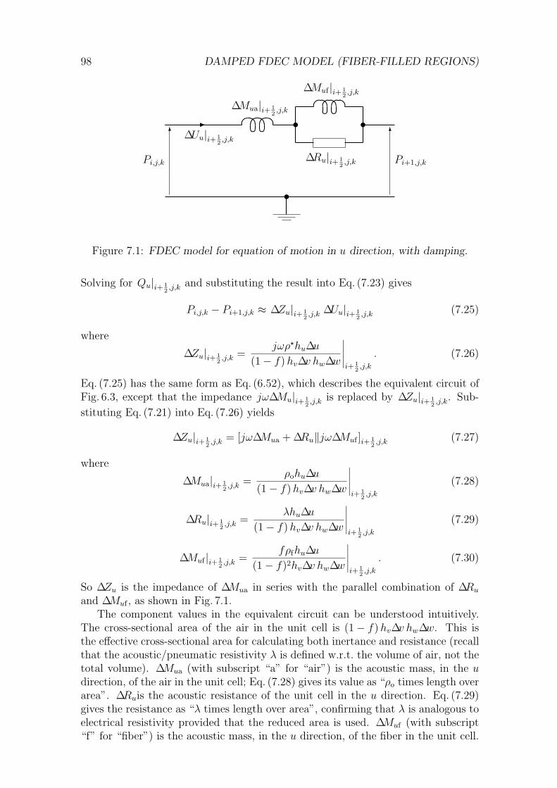
98 DAMPED FDEC MODEL (FIBER-FILLED REGIONS)
-
t
tt66
Pi+1,j,kPi,j,k ∆Ru|i+ 12 ,j,k
∆Muf |i+ 12 ,j,k
∆Mua|i+ 12 ,j,k
∆Uu|i+ 12 ,j,k
Figure 7.1: FDEC model for equation of motion in u direction, with damping.
Solving for Qu|i+ 12 ,j,k and substituting the result into Eq. (7.23) gives
Pi,j,k − Pi+1,j,k ≈ ∆Zu|i+ 12 ,j,k ∆Uu|i+ 1
2 ,j,k (7.25)
where
∆Zu|i+ 12 ,j,k =
jωρ?hu∆u(1− f) hv∆v hw∆w
∣
∣
∣
∣
∣
i+ 12 ,j,k
. (7.26)
Eq. (7.25) has the same form as Eq. (6.52), which describes the equivalent circuit ofFig. 6.3, except that the impedance jω∆Mu|i+ 1
2 ,j,k is replaced by ∆Zu|i+ 12 ,j,k. Sub-
stituting Eq. (7.21) into Eq. (7.26) yields
∆Zu|i+ 12 ,j,k = [jω∆Mua + ∆Ru‖jω∆Muf ]i+ 1
2 ,j,k (7.27)
where
∆Mua|i+ 12 ,j,k =
ρohu∆u(1− f) hv∆v hw∆w
∣
∣
∣
∣
∣
i+ 12 ,j,k
(7.28)
∆Ru|i+ 12 ,j,k =
λhu∆u(1− f) hv∆v hw∆w
∣
∣
∣
∣
∣
i+ 12 ,j,k
(7.29)
∆Muf |i+ 12 ,j,k =
fρfhu∆u(1− f)2hv∆v hw∆w
∣
∣
∣
∣
∣
i+ 12 ,j,k
. (7.30)
So ∆Zu is the impedance of ∆Mua in series with the parallel combination of ∆Ru
and ∆Muf , as shown in Fig. 7.1.The component values in the equivalent circuit can be understood intuitively.
The cross-sectional area of the air in the unit cell is (1− f) hv∆v hw∆w. This isthe effective cross-sectional area for calculating both inertance and resistance (recallthat the acoustic/pneumatic resistivity λ is defined w.r.t. the volume of air, not thetotal volume). ∆Mua (with subscript “a” for “air”) is the acoustic mass, in the udirection, of the air in the unit cell; Eq. (7.28) gives its value as “ρo times length overarea”. ∆Ruis the acoustic resistance of the unit cell in the u direction. Eq. (7.29)gives the resistance as “λ times length over area”, confirming that λ is analogous toelectrical resistivity provided that the reduced area is used. ∆Muf (with subscript“f” for “fiber”) is the acoustic mass, in the u direction, of the fiber in the unit cell.

7.1. EQUATION OF MOTION: COMPLEX DENSITY 99
If the effective density of the fiber is taken as the mass per unit volume of air, i.e.fρf/(1− f), then multiplying this by the length and dividing by the effective cross-sectional area gives a result agreeing with Eq. (7.30). The use of “effective density”thus explains the square in the denominator of ∆Muf . For an alternative explanation,we can evaluate ∆Mua and ∆Muf using Eq. (2.26), which gives the inertance as thetotal enclosed mass divided by the square of the cross-sectional area. It is also worthnoting that ∆Mua and ∆Muf are in the ratio of (1− f)ρo to fρf , i.e. the ratio of thedensity of the air to the density of the fiber when both densities are w.r.t. overallvolume.
The topology of the equivalent circuit is also quite intuitive. To move the air inthe unit cell, the pressure difference must overcome the inertia of the air plus theimpedance of the fiber; hence ∆Mua appears in series with the elements representingthe fiber. To overcome the impedance of the fiber, the air can either flow throughthe fiber (which has resistance ∆Ru) or move the fiber (which has inertance ∆Muf)and the fluxes due to these two effects are additive; hence ∆Ru and ∆Muf are inparallel.
The equivalent circuit also yields a physical description of the high- and low- fre-quency behavior of the air and fiber. At low frequencies, most of the total flux flowsthrough ∆Muf (moving with the fiber) rather than through ∆Ru (moving throughthe fiber), indicating that the motion of the fiber almost keeps up with that of theair (remember that the term “flux” refers to the motion of the air only). At high fre-quencies, most of the total flux is carried by ∆Ru, indicating that the fiber remainsalmost stationary while the air moves through it. This conclusion agrees with thatof Bradbury [13, p. 163], who uses a physical argument based on the “time taken forthe fibrous material to be set in motion” by the air passing through it.
7.1.4 Computation of mass elements
The component values of the equivalent circuit in Fig. 7.1 may be found in practiceusing equations (7.28) to (7.30), provided that ρo, ρf , f and λ are known.
The density ρo, in common with all the other acoustical properties of air, canbe calculated with acceptable accuracy from T and P0. Algebraic formulae for anumber of such properties are developed, in an appropriate computational order,in Chapter 9. Using these formulae, one can produce acoustic simulation softwarewhich requires the user to specify the ambient temperature and pressure and com-putes all the required properties of air therefrom; this is convenient for the user andminimizes the risk of erroneous or inconsistent data.
The intrinsic glass density ρf and the average glass density fρf are specificationsof the fibrous filling material; dividing the second by the first gives f . In a bale oflow-density fiberglass, the mass of the air is not a negligible part of the total mass.Therefore, if fρf is measured by weighing a known volume of the material, it isimportant to weigh only the glass and not also the air between the fibers. Fortunatelythe correct weight is measured almost by default, because the air between the fibersis buoyed up by the surrounding air. Of course the glass is also buoyed up—as isanything else weighed in air, including the known masses on the other side of thebalance—but for materials of typical density, such as glass, the effect of buoyancyis negligible.
The interesting quantity in equations (7.28) to (7.30) is the pneumatic resistivity

100 DAMPED FDEC MODEL (FIBER-FILLED REGIONS)
λ. The pneumatic resistance of a cylindrical sample of fiber with length L and (total)cross-sectional area A is given by
R =λL
(1− f) A(7.31)
(cf. Eq. (7.29)). Solving for λ gives
λ =(1− f) AR
L. (7.32)
By passing air through a sample of fiber and measuring the pressure drop and flux,one can find R and hence λ. Bradbury [13, pp. 164–5] has compared a number ofsuch measurements with a theoretical model to produce the semi-empirical formula
λ ≈ 27 ηf 1.4
d2 (7.33)
where η is the dynamic viscosity of air and d is the fiber diameter. Unfortunatelythere is considerable uncertainty in the proportionality factor 27. It is clear, however,that λ is proportional to η and depends on ambient temperature and pressure just asη does. Therefore even a measurement of λ under particular ambient conditions willnot be valid under other conditions unless it is corrected for the change in η. Hence,whether one determines λ using Eq. (7.33) or by experiment, it is necessary to knowη as a function of temperature and pressure. In fact η is remarkably insensitive topressure and may be regarded as a function of temperature alone. For a wide rangeof temperatures, including any likely to be encountered in a listening room, η maybe calculated from Eq. (9.10), given in Chapter 9.
In Chapter 10, Eqs. (7.33) and (9.10) will be used to obtain reasonable valuesof λ for the purpose of illustration. But it should be remembered that, becauseof the uncertainty in the proportionality factor and the possibility that λ may beanisotropic, Eq. (7.33) is the least accurate formula used in this thesis.
7.2 Equation of compression: complex gamma
In free air, i.e. without fibrous filling, Eq. (6.57) gives a relation between pressure anddensity in phasor form. Because pressure and density are related to temperature,and because temperature differences tend to decay due to heat conduction, we wouldexpect the presence of heat-absorbent fiber to alter the pressure-density relation ina frequency-dependent manner, so that the new relation could be described simplyby replacing γ with a frequency-dependent complex quantity γ?; that is
P =γ?P0
ρoρe. (7.34)
We shall see that the equation of compression in the presence of fiber can indeed bewritten in this form, and leads to a simple modification to the compliance elements ofthe finite-difference equivalent circuit. The form of the modified circuit is as intuitiveas for the equation of motion, although the component values are not. Nevertheless,the components have physical significance; for example, two RC time constants inthe equivalent circuit correspond to thermal time constants in the air-fiber system.

7.2. EQUATION OF COMPRESSION: COMPLEX GAMMA 101
At this point it can be seen how γ? is related to Arai’s complex bulk modulus [2,p. 17]. In Eq. (7.34), the phasor representation of fractional compression is ρe/ρo.So the complex bulk modulus, defined as the ratio of the pressure phasor to thefractional compression phasor, is γ?P0. This is the same as the adiabatic bulkmodulus for undamped air except that γ? replaces γ.
7.2.1 Thermal and mechanical definitions of γ
The finite-difference model of compression in fiber-filled enclosures draws heavilyon the thermodynamics of ideal gases. The present subsection prepares for thisby applying conservation of energy to the adiabatic compression of air, withoutfiber, to verify that γ as defined by Eq. (6.57) is indeed the “ratio of specific heats”referred to in Subsection 2.2.4. Then Subsection 7.2.2 finds an expression in termsof specific heats for the γ? of a fiber-filled region. Whereas the present subsectionbegins with a thermal definition of γ and derives a mechanical definition (namelyEq. (6.57)), Subsection 7.2.2 proceeds in the opposite direction. In both cases, thethermal definition is needed for calculating γ or γ?, while the mechanical definitionis needed for deriving the acoustic equation of compression.
In a sample of an ideal gas, let pt be the pressure, v the specific volume and u thespecific internal energy, where “specific” means “per unit mass”. Then the specificenthalpy h is defined as
h = u + ptv. (7.35)
If T is the absolute temperature, the specific heats are defined as [9, p. 138]
Cp =∂h∂t
∣
∣
∣
∣
∣ constant pt
(7.36)
and
Cv =∂u∂t
∣
∣
∣
∣
∣ constant v. (7.37)
Now an ideal gas is modeled by the familiar equation of state
ptv = RT (7.38)
where R is the gas constant on a mass basis (see Subsection 2.2.4), so Eq. (7.35)may be rewritten
h = u + RT. (7.39)
Another property of an ideal gas, less familiar but more fundamental than theequation of state, is that the specific internal energy u of a given gas is a functionof temperature alone [9, pp. 135–7]. Therefore the “constant v” condition in thedefinition of Cv may be replaced by any other condition, including constant pt.Using this fact, we can differentiate Eq. (7.39) w.r.t. T at constant pt, obtaining theuseful result
Cp = Cv + R (7.40)
which relates the specific heats of an ideal gas.Now γ is initially defined as
γ = Cp/Cv (7.41)

102 DAMPED FDEC MODEL (FIBER-FILLED REGIONS)
wherefore it is called the ratio of specific heats. Substituting from Eq. (7.40) leadsto the alternative definition
γ =Cv + R
Cv(7.42)
which is valid for ideal gases only.Eq. (7.42) is a thermal definition of γ. But for acoustical purposes we also require
a mechanical definition of γ in terms of the behavior of the medium in compression.Now consider a sample of ideal gas subject to adiabatic compression. Since there
is no heat transfer, the change in internal energy of the gas is equal to the workdone on the gas, which is minus the work done by the gas. That is, in terms ofdifferential increments of work and energy per unit mass,
Cv dT = −pt dv. (7.43)
From the ideal gas equation,T =
pt
ρR. (7.44)
Differentiating this using either the quotient rule or the chain rule for partial deriva-tives, we obtain
dT =1
ρRdpt −
pt
Rdρρ2 . (7.45)
Furthermore,v = 1/ρ (7.46)
so thatdv = −dρ/ρ2. (7.47)
Also recall that pt = P0 + p, where P0 is the equilibrium pressure, so that dp = dpt.So we can substitute for dT and dv in Eq. (7.43), let pt → P0 and ρ → ρo (for smallcompressions), write dp for dpt, and solve for dp. The result is
dp =Cv + R
Cv
P0
ρodρ (7.48)
or, using Eq. (7.42),
dp = γP0
ρodρ. (7.49)
Two interesting points follow from this result. First, we can rewrite it in theform
dpP0
= γdρρo
which shows that γ is the sensitivity of pressure to density. Thus γ has a mechanicaldefinition that can be concisely expressed in words. Second, if we divide both sidesof Eq. (7.49) by dρ and recall that
dpdρ
= c2
(Eq. (2.31)), we find an expression for c2 agreeing with Eq. (2.39). Thus we havean alternative derivation of Eq. (2.39) which is independent of Eq. (2.37) and itssupporting reference to Barrow [9, pp. 139–40].

7.2. EQUATION OF COMPRESSION: COMPLEX GAMMA 103
Returning to the main problem, if we consider p and ρ to be functions of time tand divide Eq. (7.49) by dt, we obtain7
p =γP0
ρoρ =
γP0
ρoρe. (7.50)
This is the same as Eq. (6.56), which leads to Eq. (6.57), which is the desired formof the mechanical definition of γ for an ideal gas. Substituting γ? for γ in Eq. (6.57)gives Eq. (7.34), which will be adopted as the definition of γ? in a fiber-filled region.It remains to convert this mechanical definition into a thermal definition in terms ofspecific heats; the thermal definition will serve as a computational formula for γ?.
7.2.2 Derivation of complex gamma
In Subsection 7.1.2, the complex density ρ? was found by eliminating the fibervelocity between two equations of motion, one for the air and the other for thefiber. The complex gamma, however, is not found by eliminating the “fiber density”between two equations of compression. The fibers are assumed to be intrinsicallyincompressible in the sense that they occupy a constant (small) volume, but infinitelycompressible in the sense that they make negligible contribution to the bulk modulusof the air-glass mixture (wherefore the rigidity of the fibers was neglected in derivingthe complex density). Thus there is only one equation of compression—that of theair in the presence of fiber. It will be derived after the complex gamma has beendetermined.
In principle, γ? is found by eliminating the air temperature and fiber temperaturebetween three equations, one expressing the first law of thermodynamics for the air,one based on the ideal gas equation, and one describing the conduction of heatbetween the air and the fiber. It is convenient at the beginning to introduce specificvolume as an additional variable, which is eliminated by an additional equationrelating specific volume and density. As in Subsection 7.1.2, the elimination ofvariables is facilitated by using phasor forms of the equations.
Consider the compression of a sample of air which is permeated by a mass of low-density fiberglass. Rapid compression, such as occurs in loudspeaker enclosures, maybe considered adiabatic from the viewpoint of an external observer, in the sense thatif the air and fiber together are considered as a system, negligible heat is conductedacross the boundary between the system and surroundings. But the compression isnot adiabatic when we consider the air alone; the fine fiber matrix has a very largesurface area per unit volume, allowing rapid conduction of heat between the fiberand the air, so that substantial heat conduction can occur during one cycle of anaudio-frequency oscillation.
When the air-fiber mixture is compressed, the work done imparts energy to themixture. Some of this energy appears as an increase in the internal energy of the air.Because the air is modeled as an ideal gas, the increase in internal energy is entirelymanifested as an increase in air temperature. The rest of the energy heats the fiber.It is assumed that the glass (or other material of which the fiber is composed) isincompressible, so that no energy is consumed in compressing the glass. It is alsoassumed, as hinted above, that there is no leakage of energy due to heat conduction
7The reader who prefers rigor to clarity may rework the derivation from Eq. (7.43) using timederivatives instead of differentials and thereby avoid “dividing by dt”.

104 DAMPED FDEC MODEL (FIBER-FILLED REGIONS)
between the air-fiber system and its surroundings. The work and energy terms willfirst be constructed on a per-unit-mass basis, as is most familiar. This will causesome quantities to be defined per unit mass of air and others per unit mass of fiber,whereas the energy balance requires all terms to have a common basis. Thereforeall terms will be converted to “per unit overall volume” before they are inserted inthe energy equation.
When the air is compressed so that its specific volume v is reduced by dv, thework done per unit mass of air is
dw = −pt dv. (7.51)
The increase in the internal energy of the air, per unit mass of air, is
du = Cv dT (7.52)
where T is the absolute temperature. To convert these two terms from a mass basisto an overall volume basis, we multiply by the average density of the air, which is
(1− f)ρ
where f is the filling factor as before. Let Cf be the specific heat of the fiber andTf the average temperature of the fiber. Then the heat transferred to the fiber, perunit mass of fiber, is
dq = Cf dTf . (7.53)
To convert this to energy per unit overall volume, we must multiply by the averagedensity of the fiber, which is
fρf .
Assembling all the terms, we find that the energy equation is
−(1− f)ρpt dv = (1− f)ρCv dT + fρfCf dTf . (7.54)
At this point it is convenient to consider all the thermodynamic variables asfunctions of time and divide through by dt, thus expressing the energy balance interms of time derivatives, i.e. as a power balance.8 Further, let T0 be the systemequilibrium temperature, i.e. the temperature of the air and fiber when the pressureis P0 and the air-fiber system is in thermal and mechanical equilibrium. Then let θand θf be the temperature rises (or excess temperatures) of the air and the fiber, sothat
T = T0 + θ (7.55)
andTf = T0 + θf . (7.56)
Then we may write θ for T and θf for Tf , so that the power balance equation becomes
−(1− f)ρptv = (1− f)ρCvθ + fρfCf θf . (7.57)
8The reader who prefers not to “divide by dt” may rework the derivation from Eq. (7.51) usingtime derivatives instead of differentials and proceeding directly to a power balance, without usingan energy balance as an intermediate step.

7.2. EQUATION OF COMPRESSION: COMPLEX GAMMA 105
As we require a relationship between p and ρ, we must eliminate all references to v,θ and θf . To this end, first note that Eqs. (7.44) and (7.46) from Subsection 7.2.1remain valid. Differentiating Eq. (7.46) w.r.t. time yields
v = −ρ/ρ2 = −ρe/ρ2. (7.58)
Substituting this into Eq. (7.57) gives
(1− f)ptρe/ρ = (1− f)ρCvθ + fρfCf θf . (7.59)
and thus eliminates v. Differentiating Eq. (7.44) w.r.t. time gives
θ = T =ρpt − ptρ
ρ2R=
ρp− ptρe
ρ2R(7.60)
which can be used to eliminate θ. Then, to eliminate θf , we need an equation de-scribing the heat conduction between the air and the fiber. Of course the conductionof heat requires a temperature gradient within both the air and the glass, so thetemperature variables mentioned so far (T, Tf , θ, θf) must be understood as spatialaverages. If we assume, as a linear approximation, that the rate of heat transfer isproportional to the difference between the average temperatures of the air and thefiber, we may write
θf =θ − θf
τa(7.61)
where τa is a constant with the dimensions of time.9
The physical meaning of τa may be found by assuming that θ in the above equa-tion is constant. Then we have a simple differential equation in θf whose solutionshave the form
θf = θ + Ae−t/τa (7.62)
where A is a constant. Thus τa is the thermal time constant between the air and thefiber when the average air temperature is held constant by an external energy source;the subscript “a” is for “air”. While the definition of τa seems clumsy, it is responsiblefor the simplicity and generality of Eq. (7.61). Because the fiber is incompressible,no work can be done on it, so that no work term complicates the equation. IfEq. (7.61) were written for θ instead of θf , it would need to include a work termor assume a specific condition such as constant volume (which involves no work)or constant pressure (for which the specific heat Cp takes work into account). ButEq. (7.61) does not require constant pressure or constant volume or even constantθ; the constant-θ assumption is used only to find a physical interpretation of τa.
Now let pt → P0 and ρ → ρo (for small compressions), and let the phasor repre-sentations of θ and θf be Θ and Θf , respectively. Then the phasor forms of equations(7.59) to (7.61) may be written
(1− f)P0ρe/ρo = (1− f)ρoCvΘ + fρfCfΘf (7.63)
Θ =ρoP − P0ρe
ρ2oR
(7.64)
9The justification for modeling the heat exchange in terms of a single time constant is given inChapter 8 (especially Subsection 8.2.6).

106 DAMPED FDEC MODEL (FIBER-FILLED REGIONS)
Θf =Θ
1 + jωτa(7.65)
(the first two equations have been divided through by jω and the third has beensolved for Θf).
It remains to eliminate Θ and Θf between the above three equations, solve forP , write the result in the form of Eq. (7.34) and extract the expression for γ?. Butobtaining γ? in a form amenable to physical interpretation requires some care. First,substituting Eq. (7.65) into Eq. (7.63) gives
(1− f)P0ρe/ρo =[
(1− f)ρoCv +fρfCf
1 + jωτa
]
Θ. (7.66)
Next, substituting for Θ from Eq. (7.64), multiplying through by ρ2oR, and grouping
the terms in ρoP on the left and the terms in P0ρe on the right, we obtain
ρoP[
(1− f)ρoCv +fρfCf
1 + jωτa
]
= P0ρe
[
(1− f)ρo(Cv + R) +fρfCf
1 + jωτa
]
. (7.67)
Finally, writing Cp for Cv + R (Eq. (7.40)) and solving for P gives
P =γ?P0
ρoρe (7.68)
(the form of Eq. (7.34)), where
γ? =(1− f)ρoCp + fρfCf/(1 + jωτa)(1− f)ρoCv + fρfCf/(1 + jωτa)
. (7.69)
7.2.3 High- and low-frequency limits of γ?
As frequency increases, the term common to the numerator and denominator ofEq. (7.69) approaches zero, so that
limω→∞
γ? =Cp
Cv= γ. (7.70)
Recall that γ? was defined so that it would reduce to γ, the ratio of specific heats, inthe case of adiabatic compression (Subsection 7.2.1). At sufficiently high frequenciesthe compression may indeed be regarded as adiabatic because there is little time forheat to conduct during one cycle. Thus the high-frequency limit of γ? agrees withphysical requirements.
The low-frequency behavior of γ? has a more complex physical explanation. Atsufficiently low frequencies, γ? may be approximated by10
γ?o4= lim
ω→0γ? =
(1− f)ρoCp + fρfCf
(1− f)ρoCv + fρfCf. (7.71)
To make sense of this expression it is necessary to define a few variants of the term“specific heat”. The heat capacity of a sample of material is the ratio of the change
10Because the system approaches thermal equilibrium as ω → 0, the definition of γ?o is consistent
with the convention that a zero subscript denotes an equilibrium value.

7.2. EQUATION OF COMPRESSION: COMPLEX GAMMA 107
in thermal energy to the change in temperature; it is an “extensive” property, beingproportional to the sample size. What has hitherto been called the specific heat ofthe sample is the mass-specific heat, i.e. the heat capacity per unit mass; it is an“intensive” property, not being dependent on the sample size. The volume-specificheat will be defined for present purposes as the heat capacity per unit overall volume;the use of overall volume, rather than the volume occupied by the air or the glass,allows the volume-specific heat of the air-glass mixture to be found by adding thevolume-specific heats of its components. Now the average densities (masses perunit overall volume) of the air and the fiber are (1− f)ρo and fρf , respectively.Hence the volume-specific heats are (1− f)ρoCp for the air at constant pressure,(1− f)ρoCv for the air at constant volume, and fρfCf for the fiber (whether theair is at constant pressure or constant volume). So in the low-frequency limit ofγ?, the numerator is the total volume-specific heat at constant pressure and thedenominator is the total volume-specific heat at constant volume. This ratio isunchanged if both specific heats are made specific to the mass of air (by dividingby (1− f)ρo). So at sufficiently low frequencies, γ? is a ratio of heat capacities perunit mass of air, in agreement with the original definition of γ (Eq. (7.41)). This isto be expected because if the air and fiber are in thermal equilibrium, they behaveas a single reservoir of heat; from the viewpoint of an external observer compressingthe air, the heat capacity of the fiber simply adds to that of the air, so that theair itself appears to have increased specific heats. Moreover, because the addedheat capacity of the fiber is the same for constant volume and constant pressure,the apparent Cp and Cv of the air still differ by R. So the air still behaves as anideal gas—and the derivation of Eq. (6.57) from the specific heats (Subsection 7.2.1)remains valid—except that γ?
o replaces γ.Thus in both the high-frequency limit and the low-frequency limit, γ? is the
ratio of the apparent specific heats of the air, satisfying the assumptions made inthe derivation of Eq. (6.57). Both limiting values, of course, are real.
From Eq. (7.71) it is easily seen that 1 < γ?o < γ. Thus it is often said that fiber
filling reduces the effective γ at low frequencies and increases the compliance (or“apparent volume”) of a bass enclosure (see e.g. Chase [14, p. 298]). Eq. (7.71) alsoindicates that γ?
o ≈ 1 if fρfCf ρoCp, i.e. if the fiber can be approximated as aninfinite heatsink. In this case, low-frequency compressions are nearly isothermal.Indeed, when γ = 1, Eq. (2.37) reduces to Boyle’s law, which holds for isothermalcompression.
7.2.4 Equation of compression and equivalent circuit
To simplify the derivation of an equivalent circuit from the expression for γ?, let ussimplify the expression itself by defining
β =fρfCf
(1− f)ρoCv. (7.72)
Then dividing the numerator and denominator of Eq. (7.69) by (1− f)ρoCv gives
γ? =γ + β/(1 + jωτa)1 + β/(1 + jωτa)
(7.73)

108 DAMPED FDEC MODEL (FIBER-FILLED REGIONS)
and taking low-frequency limits gives
γ?o =
γ + β1 + β
. (7.74)
This form of γ?o can still be understood as a ratio of specific heats. In Eq. (7.72),
the numerator is the volume-specific heat of the fiber and the denominator is thevolume-specific heat of the air at constant volume. Thus β is the normalized volume-specific heat of the fiber, when the volume-specific heat of the air at constant volumeis assigned a value of unity. Similarly, γ is the normalized volume-specific heat ofthe air at constant pressure. So in Eq. (7.74), the numerator is the total normalizedvolume-specific heat at constant pressure and the denominator is the total normal-ized volume-specific heat at constant volume.
From Eq. (6.61), note that the compliance element ∆Ci,j,k is proportional to 1/γ,so that the associated acoustic admittance is proportional to jω/γ. This suggeststhat we should find an expression for jω/γ? involving the harmonic sum operator“‖”, which in this case will apply to admittances in series rather than impedances inparallel. Taking reciprocals of both sides of Eq. (7.73) and multiplying by jω, thenmultiplying the numerator and denominator by the factor (1 + jωτa), we obtain
jωγ? = jω
1 + jωτa + βγ(1 + jωτa) + β
. (7.75)
Expressing the right-hand side in series-parallel form is straightforward if we noticethat the third term of the numerator may be partitioned into two terms so that thefirst three terms of the new numerator are together a multiple of the denominator:
jωγ? = jω
1 + jωτa + βγ + γ−1
γ β
γ(1 + jωτa) + β
= jω[
1γ
+γ − 1
γβ
γ(1 + jωτa) + β
]
=jωγ
+β(γ − 1)
γjω
γ + β + jωτaγ. (7.76)
Now we can multiply and divide the right-hand term by (γ + β)τaγ, obtaining aharmonic sum for the second factor, and apply the distributive law:
jωγ? =
jωγ
+β(γ − 1)
γ(γ + β)τaγ(γ + β) jωτaγ
(γ + β) + jωτaγ
=jωγ
+β(γ − 1)
γ2τa(γ + β)[(γ + β) ‖ jωτaγ]
=jωγ
+β(γ − 1)
γ2τa
∥
∥
∥
∥
∥
jωβ(γ − 1)γ(γ + β)
. (7.77)
Derivation of an equivalent circuit requires a finite-difference approximation tothe equation of compression in a fiber-filled region. Whereas the definition of ρ? isthe phasor form of the equation of motion (Eq. (7.1)), the present definition of γ?
(Eq. (7.34)) is not a form of the equation of compression (Eq. (6.58)). The phasorform of the equation of compression in a fiber-filled region must be derived from

7.2. EQUATION OF COMPRESSION: COMPLEX GAMMA 109
the equation of continuity in its most general integral form. In other words wemust return to first principles—and again acknowledge and justify the linearizingapproximations. But the task can be expedited by exploiting previous results.
Consider a control volume V enclosed by a stationary surface σ with outwardunit normal vector n. Conservation of air requires that the time rate of change ofmass inside V be minus the total mass flux outward through σ. For the purpose ofcalculating the mass of air in V and the mass flux of air out of V in the presence offiber filling, the effective density of air is (1− f)ρ. Alternatively, we may considerthe effective volume of V and surface area of σ to be modified by the factor (1− f),and take the effective density as ρ. In either case, the equation of continuity is
ddt
∫∫∫
V(1− f)ρ dV = −
∫∫
σ© (1− f)ρq .n dσ. (7.78)
When both the air and the fiber are in motion, the fractional variations in f maybe of similar magnitude to those in ρ. Variations in ρ are are not negligible in theequation of continuity, because ρ is the only time-varying quantity under the volumeintegral in the free-air form of the equation (Eq. (2.27)). But because f is small,the fractional variations in (1− f) are small compared with those in f and hence inρ. Fractional variations in q are of course much larger again. Hence, in Eq. (7.78),it is reasonable to treat (1− f) as a constant and take it outside the integral anddifferential operators, where it cancels. Thus Eq. (7.78) reduces to Eq. (2.27), theequation of continuity in the absence of fiber.
As the familiar equation of continuity still holds (to an acceptable approxima-tion), so too do Eqs. (2.30) and (6.54) which are derived therefrom. Multiplyingboth sides of Eq. (6.54) by γ?P0/ρo and using Eq. (7.34) to rewrite the left-hand sidein terms of P , we obtain
jωP = −γ?P0 divQ. (7.79)
This result is the phasor form of the equation of compression, identical to Eq. (6.58)except that γ? replaces γ. Thus γ? can be defined by a modified equation of com-pression just as ρ? is defined by a modified equation of motion.
Eq. (7.79) is the starting point for the finite-difference approximation. Hence theequivalent circuit derivation will be almost identical to the argument from Eq. (6.58)to Eq. (6.66), and need not be repeated in full. The presence of fiber means that thevolume element ∆V i,j,k will contain an extra factor (1− f). The same factor willappear in the complex admittance element ∆Y i,j,k, which corresponds to jω∆Ci,j,k
in Eq. (6.66). Hence, in deriving Eq. (6.63), we will multiply the numerator anddenominator of Eq. (6.59) by (1− f)∆u∆v∆w. The factor (1− f) will appear on theright of Eq. (6.63), but will be included in ∆Y on the left. Now because the effectiveareas of the faces of the volume element are modified by the factor (1− f), thisfactor must be included in the definitions of the fluxes ∆Uu|i+ 1
2 ,j,k, etc. So the extra(1− f) on the right of Eq. (6.63) is absorbed into the flux terms, leaving Eq. (6.66)unchanged, although the terms in it have been redefined. The new estimated fluxesare
∆Uu|i+ 12 ,j,k = [(1− f) hv∆v hw∆w Qu]i+ 1
2 ,j,k (7.80)
∆Uu|i− 12 ,j,k = [(1− f) hv∆v hw∆w Qu]i− 1
2 ,j,k (7.81)
and similarly for the ∆Uv and ∆Uw terms. The new estimated volume element is
∆V i,j,k = [(1− f) hu∆uhv∆v hw∆w]i,j,k (7.82)
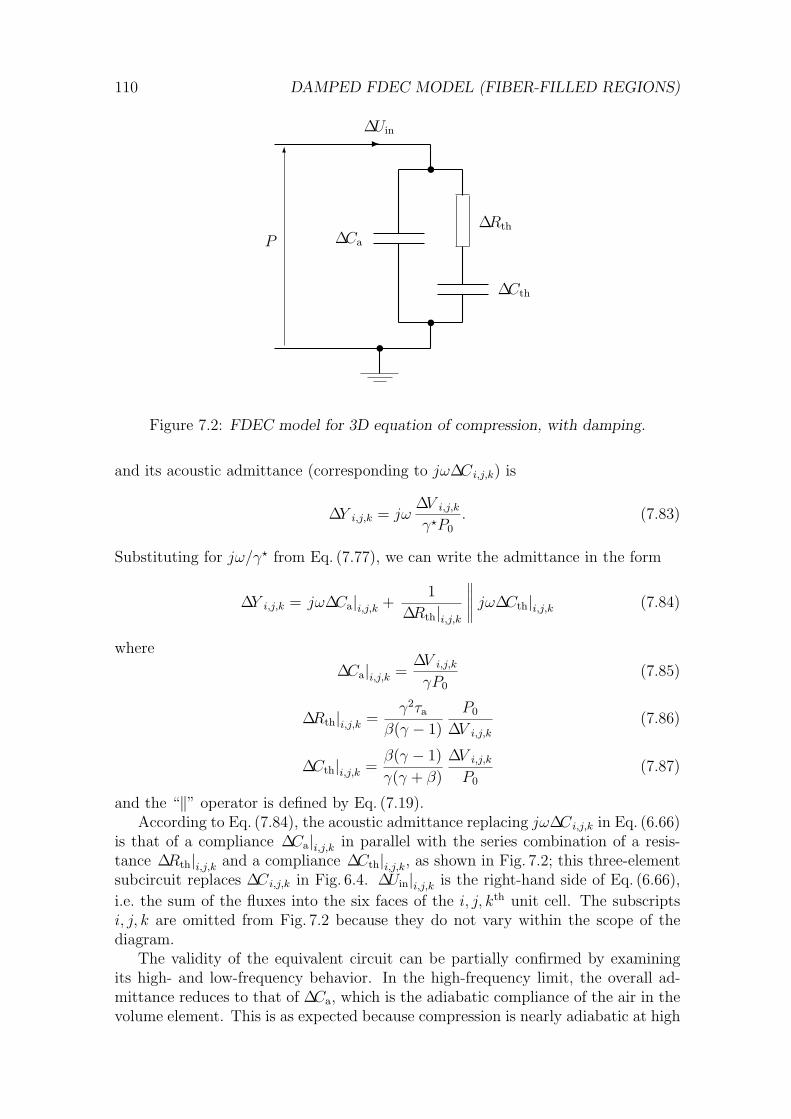
110 DAMPED FDEC MODEL (FIBER-FILLED REGIONS)
-6
t t
t∆Ca
∆Uin
P
∆Cth
∆Rth
Figure 7.2: FDEC model for 3D equation of compression, with damping.
and its acoustic admittance (corresponding to jω∆Ci,j,k) is
∆Y i,j,k = jω∆V i,j,k
γ?P0. (7.83)
Substituting for jω/γ? from Eq. (7.77), we can write the admittance in the form
∆Y i,j,k = jω∆Ca|i,j,k +1
∆Rth|i,j,k
∥
∥
∥
∥
∥
jω∆Cth|i,j,k (7.84)
where∆Ca|i,j,k =
∆V i,j,k
γP0(7.85)
∆Rth|i,j,k =γ2τa
β(γ − 1)P0
∆V i,j,k(7.86)
∆Cth|i,j,k =β(γ − 1)γ(γ + β)
∆V i,j,k
P0(7.87)
and the “‖” operator is defined by Eq. (7.19).According to Eq. (7.84), the acoustic admittance replacing jω∆Ci,j,k in Eq. (6.66)
is that of a compliance ∆Ca|i,j,k in parallel with the series combination of a resis-tance ∆Rth|i,j,k and a compliance ∆Cth|i,j,k, as shown in Fig. 7.2; this three-elementsubcircuit replaces ∆Ci,j,k in Fig. 6.4. ∆Uin|i,j,k is the right-hand side of Eq. (6.66),i.e. the sum of the fluxes into the six faces of the i, j, kth unit cell. The subscriptsi, j, k are omitted from Fig. 7.2 because they do not vary within the scope of thediagram.
The validity of the equivalent circuit can be partially confirmed by examiningits high- and low-frequency behavior. In the high-frequency limit, the overall ad-mittance reduces to that of ∆Ca, which is the adiabatic compliance of the air in thevolume element. This is as expected because compression is nearly adiabatic at high

7.2. EQUATION OF COMPRESSION: COMPLEX GAMMA 111
frequencies. In the low-frequency limit, the overall admittance is that of ∆Ca and∆Cth in parallel. Adding the two compliances using a common denominator gives
∆Ca|i,j,k + ∆Cth|i,j,k =∆V i,j,k
P0
1 + βγ + β
=∆V i,j,k
γ?oP0
(7.88)
where γ?o is the ratio of total specific heats at thermal equilibrium, as given by
Eq. (7.74). Thus γ?o replaces γ in the expression for the compliance of each element.
And because γ?o < γ, while ∆V is almost the same as for an undamped region, the
presence of fiber filling increases the compliance of each element at low frequencies,as stated in Subsection 7.2.3.
7.2.5 Thermal time constants from the acoustic circuit
The only thermal time constant considered so far is τa, which according to Eq. (7.62)is the thermal time constant when the average air temperature is held constant. Thisdefining condition is not realistic. Moreover it cannot be expressed as a boundarycondition for the heat equation, so the resulting time constant cannot be determinedby the usual methods for solving partial differential equations. In Chapter 8 it willbe seen that the easiest time constant to calculate is τfp, which applies to constantfiber temperature and constant air pressure. A related constant is τfv, which appliesto constant fiber temperature and constant air volume. To relate τfp and τfv toτa, we must first find expressions in terms of τa for τp and τv, where τp and τv arethe thermal time constants between the air and the fiber, at constant pressure andconstant volume respectively, in the absence of external heat flow. (In the definitionsof τp and τv, neither the air temperature nor the fiber temperature is constant, sothere is no subscript “a” or “f”.)
In this subsection, the acoustic circuit of Fig. 7.2 will be used to express τfp, τfv,τp and τv in terms of τa. Inverting the first of these results will enable all timeconstants to be expressed in terms of τfp, which in turn can be expressed in terms ofthe filament diameter and filling factor using a formula to be derived in Chapter 8.
First we find τp, which applies to constant pressure.11 In Fig. 7.2, the excesspressure p appears in (or “across”) ∆Ca. If this pressure is constant, no flux flowsin ∆Ca, so that all of the external flux ∆Uin flows in ∆Rth and ∆Cth; that is, whenthe air expands, the volume of air flowing out of the volume element is supplied by“discharging” ∆Cth, so that the pressure in ∆Cth is proportional to minus the excessvolume. But at constant pressure, specific volume is proportional to temperature,so that the excess volume is proportional to the excess temperature θ. Thereforethe pressure in ∆Cth is proportional to −θ, so that the thermal time constant is justthe time constant of ∆Rth and ∆Cth; that is
τp = ∆Rth ∆Cth. (7.89)
Substituting from Eqs. (7.86) and (7.87) gives
τp =γτa
γ + β. (7.90)
11Leach explicitly assumes that the heat exchange takes place at constant pressure [30, p. 588 andFig. 3(b)], so his time constant “τf” is identical with the above “τp”. His subscript “f” (in Romantype) apparently stands for constant force, which implies constant pressure. Here the subscript“f” (in Roman type) stands for constant fiber temperature, while the unsubscripted “f” (in italictype) is the filling factor.
112 DAMPED FDEC MODEL (FIBER-FILLED REGIONS)
Next we find τv. At constant volume (or constant density), the pressure andtemperature of the air are proportional, so that the excess pressure appearing across∆Ca (in Fig. 7.2) is proportional to the excess air temperature θ. Therefore thethermal time constant is the time constant applicable to the pressure across ∆Ca.Now at constant volume there is no external flux into the admittance element (thatis, ∆Uin = 0), so that the equivalent circuit is isolated and its time constant is simplythat of the series C-R-C circuit; that is
τv = ∆Rth(∆Ca‖∆Cth). (7.91)
Substituting from the above formulae for ∆Rth, ∆Ca and ∆Cth, then taking allfactors of ∆Rth except γτa inside the harmonic sum and canceling where possible,we obtain12
τv = γτa
(
1β(γ − 1)
∥
∥
∥
∥
∥
1γ + β
)
=τa
1 + β. (7.92)
Now the time constants τfp and τfv are special cases of τp and τv, respectively, forwhich the fiber temperature is held constant. One way to achieve this condition isto assume that the fiber is an infinite heatsink, i.e. that β, the normalized volume-specific heat of the fiber, is infinite. But we cannot simply let β →∞ in Eqs. (7.90)and (7.92), because τa depends on β—the time taken to cause a given change in thetemperature of the fiber depends on its specific heat, and indeed becomes infiniteas β →∞. So let us define
∆Cth f = limβ→∞
∆Cth. (7.93)
From Eq. (7.87) the limit is found to be
∆Cth f =γ − 1
γ∆V i,j,k
P0. (7.94)
Comparing this with Eq. (7.85), we see that ∆Cth f = (γ − 1) ∆Ca ≈ 0.4 ∆Ca. So ifthe fiber is an infinite heatsink as assumed by Chase [14], and if the frequency islow so that ∆Cth f is effectively in parallel with ∆Ca, and if the filling factor is smallso that the reduction in air volume is negligible, then the presence of fiber fillingincreases the compliance by 40%, as implied by Chase’s Figs. 2 and 3.
Using Eqs. (7.89) and (7.91) with ∆Cth f in place of ∆Cth, we obtain
τfp =γτa
β(7.95)
and
τfv = γτa
(
1β(γ − 1)
∥
∥
∥
∥
∥
1β
)
=τa
β. (7.96)
Now, to express all the time constants in terms of τfp, we solve Eq. (7.95) for τa,obtaining
τa =βτfp
γ, (7.97)
12The middle expression in Eq. (7.92) is simplified by noting that the harmonic sum of twofractions with the same numerator is the common numerator over the sum of the denominators;this is easily proven from the definition.

7.2. EQUATION OF COMPRESSION: COMPLEX GAMMA 113
and substitute for τa in Eqs. (7.96), (7.90) and (7.92). The results are
τfv =τfp
γ(7.98)
τp =βτfp
γ + β(7.99)
τv =βτfp
γ(1 + β). (7.100)
(In Eq. (7.99), notice that τp < τfp. Leach [30, p. 592] uses τfp (which he calls τ1) asan estimate of τp (which he calls τf) and notes that it is an overestimate, resultingin a conservative estimate of the bandwidth over which the compression can beassumed “isothermal”.)
Of the formulae for the component values in Fig. 7.2, the only one containing atime constant is Eq. (7.86); substituting Eq. (7.97) into Eq. (7.86) gives
∆Rth|i,j,k =γτfp
γ − 1P0
∆V i,j,k(7.101)
which is simpler than the original expression in terms of τa.
7.2.6 Thermal time constants from the heat circuit
The relations between the five thermal time constants will now be verified using aconventional heat circuit. Although this exercise does not yield any new results,it confirms the derivation of the four equations (7.97) to (7.100) from the acousticcircuit (Fig. 7.2), providing further evidence that the acoustic circuit is correct.
At constant pressure, the heat capacities per unit overall volume are (1− f)ρoCp
for the air and fρfCf for the fiber. Suppose that, starting from thermal equilibrium,we somehow transfer heat from the fiber to the air. Let q denote the transferredenergy per unit overall volume. Then for the air,
q = (1− f)ρoCp θ , (7.102)
and for the fiber,−q = fρfCf θf , (7.103)
where the excess temperatures θ and θf are spatial averages. So if heat energy perunit volume is represented by charge and excess temperature by voltage, the abovetwo equations show that the volume-specific heats are analogous to capacitances.Now let Gth denote the thermal conductance per unit overall volume between theair and the fiber (assuming that the rate of heat transfer is proportional to thetemperature difference and to the air-glass surface area, the latter being proportionalto overall volume). Then
q = Gth(θf − θ) (7.104)
so that Gth is analogous to electrical conductance.Eqs. (7.102) to (7.104) are modeled by the heat circuit shown in Fig. 7.3. Ground
potential represents the equilibrium temperature T0. Nodal temperatures are rel-ative to T0 and are written “in the nodes”. The conductance Gth is shown as aresistance 1/Gth.

114 DAMPED FDEC MODEL (FIBER-FILLED REGIONS)
fρfCf(1− f)ρoCp
θ θf
1/Gth q
Figure 7.3: Air-fiber heat circuit at constant pressure.
From the figure, the constant-pressure thermal time constant between the airand the fiber is
τp =1
Gth[(1− f)ρoCp‖fρfCf ] . (7.105)
Now τfp is the value of τp when θf is constant. To impose constant θf , we can either“short out” fρfCf in Fig. 7.3 or let Cf →∞ in Eq. (7.105). In either case, the resultis
τfp =1
Gth(1− f)ρoCp. (7.106)
At constant volume, the heat circuit is the same as Fig. 7.3 except that Cv
replaces Cp. Making the same replacement in Eqs. (7.105) and (7.106) gives
τv =1
Gth[(1− f)ρoCv‖fρfCf ] . (7.107)
τfv =1
Gth(1− f)ρoCv. (7.108)
Recall that τa was defined as the thermal time constant at constant air temper-ature, i.e. at constant θ. So τa can be found from the heat circuit by shorting outthe heat capacity of the air, or from Eq. (7.105) or Eq. (7.107) by letting Cp or Cv
approach infinity. The result is
τa =1
GthfρfCf . (7.109)
Checking the ratios between the time constants given by Eqs. (7.105) to (7.109)is straightforward if one remembers that Cp = γCv, that β is defined by Eq. (7.72),and that multiplication and division are distributive over harmonic addition. FromEqs. (7.109) and (7.106),
τa
τfp=
fρfCf
(1− f)ρoCp=
fρfCf
γ (1− f)ρoCv=
βγ
(7.110)
which agrees with Eq. (7.97). From Eqs. (7.108) and (7.106),
τfv
τfp=
Cv
Cp=
1γ
(7.111)
which agrees with Eq. (7.98). From Eqs. (7.105) and (7.106),
τp
τfp= 1
∥
∥
∥
∥
∥
fρfCf
(1− f)ρoCp= 1
∥
∥
∥
∥
∥
fρfCf
γ (1− f)ρoCv= 1
∥
∥
∥
∥
∥
βγ
=1γ
(γ‖β) =β
γ + β(7.112)

7.2. EQUATION OF COMPRESSION: COMPLEX GAMMA 115
which agrees with Eq. (7.99). From Eqs. (7.107) and (7.106),
τv
τfp=
1γ
∥
∥
∥
∥
∥
fρfCf
(1− f)ρoCp=
1γ
∥
∥
∥
∥
∥
fρfCf
γ (1− f)ρoCv=
1γ
∥
∥
∥
∥
∥
βγ
=1γ
(1‖β) =β
γ(1 + β)(7.113)
which agrees with Eq. (7.100).
7.2.7 Acoustic circuit from thermal time constants?
The reader has probably found that Subsection 7.2.6 is easier to understand thanSubsection 7.2.5, i.e. that the relations between the thermal time constants areeasier to derive from the heat circuit than from the acoustic circuit. Moreover, thederivation from the acoustic circuit depends on the the component values, whosedetermination has taken most of Section 7.2. But in Subsection 7.2.5, the argumentshowing that τp and τv can be read from the acoustic circuit (Fig. 7.2) depends onlyon the form of the circuit, and not on the component values.
The form of the acoustic circuit is readily established from the following intuitiveargument. At high frequencies the circuit must reduce to the adiabatic compliance∆Ca (whose value, as is well known, is given by Eq. (7.85)). If the air is subjectto a step-reduction in volume, the initial compression is adiabatic; but then theheat of compression is conducted from the air to the fiber, causing the pressure todecrease and approach a limit as the system approaches thermal equilibrium. Thusthe compliance increases as frequency decreases, approaching a limit as frequencyapproaches DC. Therefore the form of the acoustic circuit must be such that anadditional compliance appears in parallel with ∆Ca at low frequencies; this thermalrelaxation compliance may be given the symbol ∆Cth. Now the obvious way to make∆Cth operative only at low frequencies is to put a resistance in series with it. If thisthermal relaxation resistance is given the symbol ∆Rth, we have the complete formof Fig. 7.2 (together with the value of ∆Ca).
From the form of the acoustic circuit, we know that the time constant of ∆Rth
and ∆Cth is τp. So, expressing τp in terms of τfp using Eq. (7.99) (which can also bederived from the heat circuit), we have
∆Rth ∆Cth =βτfp
γ + β. (7.114)
Also from the form of the acoustic circuit, we know that the time constant of thecomplete series C-R-C circuit is τv. So, expression τv in terms of τfp using Eq. (7.100)(which can also be derived from the heat circuit), we have
∆Rth(∆Ca‖∆Cth) =βτfp
γ(1 + β). (7.115)
Thus we have two equations in the two unknowns ∆Rth and ∆Cth. The solutions are
∆Rth =τfp
(γ − 1)∆Ca(7.116)
and
∆Cth =(γ − 1)β∆Ca
γ + β. (7.117)

116 DAMPED FDEC MODEL (FIBER-FILLED REGIONS)
These results are easily confirmed using Eqs. (7.85), (7.87) and (7.101).
At this point it is convenient to compare the results of the present section withthe damped compliance circuit given by Leach [30]. Whereas Eqs. (7.85), (7.116)and (7.117) are derived in the context of the finite-difference method, Leach merelygives an equivalent circuit for a lumped total volume VB, in which the fibers displacea volume Vf . Although Leach defines a complex density to describe the inertial prop-erties of the fiber-damped air, he does not define a complex gamma or complex bulkmodulus to describe the compressibility. While he derives his complex density fromthe equations of motion for the air and the fiber, he does not derive his dampedcompliance circuit from the differential equations describing the compression andheat conduction. Instead, he determines the thermal-equilibrium compliance byassuming an adiabatic initial compression followed by an isobaric transfer of heat,then assumes that in response to a step-change in pressure, the “apparent volume”of the box begins at the adiabatic value and exponentially approaches the thermal-equilibrium value. This “step response of the volume” is Laplace-transformed, con-verted to an impulse response, and finally converted from a volume to an admittance.So Leach’s approach is less rigorous than the one used in the present section. Nev-ertheless, the results obtained above can be reconciled with Leach’s work using thefollowing identities or notational conversions:
VB(1− Vf/VB) → ∆V i,j,k
ρoc2 = γP0
CAB1 → ∆Ca|i,j,kCAB2 → ∆Cth|i,j,k
VB
Vf→ 1
fRAB1 → ∆Rth|i,j,k
τf → τp =βτfp
γ + β.
With the above seven substitutions, Leach’s Eq. (17) directly yields Eq. (7.85), whilehis Eq. (18) yields Eq. (7.117) with the aid of Eq. (7.72) and his Eq. (19) yieldsEq. (7.116) with the aid of Eq. (7.117). The only inaccuracy in Leach’s results (whichhe acknowledges) is his use of τfp as an estimate of τp; this is corrected in the lastof the above substitutions, which quotes Eq. (7.99).
7.2.8 Computation of compliance elements
If we wish to calculate ∆Ca, ∆Rth and ∆Cth using Eqs. (7.82), (7.85), (7.116)and (7.117), the quantities which must be known (other than those already dis-cussed in Subsection 7.1.4) are γ, β and τfp.
Chapter 9 includes an expression for γ in terms of Cp, which is taken as a constantfor air (see Eqs. (9.3) and (9.4)). It is therefore convenient to express β in terms ofCp also; substituting Cp/γ for Cv in Eq. (7.72), we obtain
β =γfρfCf
(1− f)ρoCp. (7.118)

7.3. TRUNCATED ELEMENTS AT BOUNDARY SURFACES 117
All parameters in this formula have been discussed already except Cf , which is aproperty of the glass. Leach [30, p. 588] gives the value Cf = 670 J kg−1 K−1.
The non-trivial part of the problem is to find τfp. Ideally we would like to com-pute the thermal time constant using a simple algebraic formula which is acceptablyaccurate for all filling factors, filament diameters, temperatures and pressures. Re-sults given in the literature are neither as simple nor as general as desired, and areinconsistent with the present author’s findings. Accordingly, the theory behind thecalculation of τfp is relegated to Chapter 8. For the moment it suffices to quote theresult, which is
τfp ≈d2
8α(m2 −m0.37) ln
(
m+12
)
(7.119)
where d is the filament diameter, α is the thermal diffusivity of air, and m = f−1/2;the estimated accuracy of the formula is 2%. Chapter 9 shows how α, like theother properties of air, can be computed from the temperature and pressure (seeEqs. (9.13) and (9.14)).
7.3 Truncated elements at boundary surfaces
In this chapter, as in Chapter 6, the use of discrete subscripts conceals the generalityof the equicoordinate surfaces bounding each volume or mass element. In Eqs. (7.28),(7.29), (7.30), (7.85), (7.86), (7.87) and the associated circuit equations, there isnothing to prevent variation of the increments ∆u, ∆v and ∆w and of the associatedcoordinates, provided that
• In the formula for a component value, scale factors are evaluated at the body-center of the element (mass or compliance);
• In a circuit equation involving a damped inertance, pressure is sampled at thecenters of two opposite faces of the element, chosen so that the normals tothe two faces are in the direction of the velocity component governed by thatelement;
• In a circuit equation involving a damped compliance, the areas of the six facesand the fluxes passing through them are calculated using the scale factors andvelocities sampled at the centers of the six faces of the element.
In the above list, word “center” refers to the midranges of the variable coordinates—two coordinates for a face-center and three for a body-center. As in Subsection 6.4.3,if we wish to interpret the names of the elements as functions of the subscripts, thename of a truncated element will contain a multiplier (usually 1
2).In Chapter 10, which considers the FDEC model of a loudspeaker enclosure
partially filled with fiber, a layer of truncated mass elements will appear againstthe diaphragm and against the walls of the enclosure; the former elements must beincluded in the model, while the latter can be ignored because they carry no flux.The boundary surface between the filled and unfilled regions will pass through a layerof inertance elements, producing two layers of truncated elements, one damped andthe other undamped.

Chapter 8
The thermal time constant τfp
In Subsection 7.2.5, the isometric and isobaric thermal time constants between theair and the fiber network are expressed in terms of a basic time constant τfp, definedas the thermal time constant for constant fiber temperature and constant pressure.In this definition, the “temperature” of the fiber means the spatial average tempera-ture. For the theoretical purposes of Subsection 7.2.5, nothing is assumed concerningthe temperature distributions within the air and the fiber. But the calculation ofτfp obviously must take these distributions into account.
First it will be shown that, at least in the case of glass fibers, the temperaturewithin each fiber1 may be assumed uniform. According to the well-known Fourierlaw of heat conduction [21, p. 4-143],
q = −κ∇T (8.1)
where q is the heat flux density (power per unit area), κ is the thermal conductivityand T is the temperature (absolute, or relative to an arbitrary reference).2 At theair-glass surface, heat is transferred between the air and the glass by the normalcomponent of q. The parallel components of q are of lesser interest; moreover, in aloudspeaker box there is no mechanism by which a substantial parallel temperaturegradient could be generated. By conservation of energy, the normal component of qis continuous across the surface. Hence a step-change in κ must be accompanied bya reciprocal step-change in the normal component of ∇T ; that is, the ∇T ratio isthe reciprocal of the κ ratio. The thermal conductivity of air at room temperatureis about 0.026Wm−1 K−1 [27, p. 962]. Common soda-lime glasses have thermalconductivities around 1 Wm−1 K−1 [31, pp. 12-143 to 146]; conductivities of othercommon glasses are of the same order of magnitude. From the figures cited, thethermal conductivity of the glass is roughly forty times that of the air, so that thetemperature gradient on the glass side of the surface is roughly one fortieth of thaton the air side. Thus it is reasonable to neglect the spatial variation of temperaturewithin the glass and assume that a “constant” glass temperature is constant anduniform.
1In this chapter it is convenient to use “fiber” to denote a single filament.2The presence of spatial derivatives in the Fourier law (Eq. (8.1)) and in the heat equation
(Eq. (8.22)) indicates that the conducting medium—air in this case—is assumed to be a continuum.Chase [14] reports a typical fiber diameter of 10 µm. According to the U.S. Standard Atmospheretables [31, p. 14-14], the molecular mean free path in air at altitudes up to 4000 m is less than10−7 m, i.e. less than one percent of the typical fiber diameter. Thus the assumption of continuityis reasonable even for the microscopic dimensions of the fibers.
118

8.1. ANALYTICAL APPROXIMATION 119
Next we must consider the pattern of heat conduction around each fiber. Supposethe air in some local region is compressed so that the air temperature rises above thefiber temperature and heat begins to flow from the air to the fibers. Over the surfaceof each fiber, the heat flux is inward. Hence, between any two fibers, there mustexist a surface across which the normal component of the heat flux density is zero;heat flows away from this surface on both sides. Let us call this surface the heatshed(by analogy with “watershed”). In the presence of many fibers, the heatshed is ahoneycomb-like surface which divides the space into a myriad of contiguous tubes,which we will naturally refer to as heat tubes. Each tube is threaded by one fiber.
In any heat tube, the maximum heat flux density, hence the maximum temper-ature gradient, occurs at the surface of the fiber. The temperature gradient is smallin the outer regions of the heat tube, reaching zero at the outer surface. Hence theposition and shape of the outer surface have little effect on the effective thermalresistance between the fiber and the air in the heat tube. Moreover, the positionand shape of the heatshed do not affect the average heat capacity of the air in aheat tube; a shift in the heatshed causes an increase in the heat capacity of one heattube and a compensating decrease in that of another. Therefore, for the purpose ofcalculating the thermal time constant, we may approximate the heatshed surround-ing each heat tube using a surface of “average shape” containing the correct averagevolume; it does not greatly matter that individual heat tubes have different shapesor volumes, or even that the heatshed may move with time.
In a sufficiently small region, each fiber may be assumed cylindrical; that is, thecurvature of the axis of each fiber may be neglected. Hence it is most convenient toassume that the surrounding heatshed is a cylindrical surface coaxial with the fiber.Let the radii of the fiber and heatshed be a and ma, respectively, where m > 1.Then the filling factor is
f =πa2
π(ma)2 = m−2 (8.2)
whencem = f−1/2. (8.3)
Subsequent analysis will use a cylindrical coordinate system coaxial with the fiberand heatshed. If r is the radial coordinate, the region of interest is a ≤ r ≤ ma.
8.1 Analytical approximation
For the typical case of a = 5µm and f = 1/400, Leach [30] calculates a transitionfrequency (fc = 1/2πτfp) of 6400Hz. For the same case, Chase [14] obtains about3.5Hz. The present author, using methods to be presented in this chapter, calculatesa transition frequency of about 289Hz. These diverse results require investigationbecause of their conflicting implications for the analysis and design of loudspeakers.In a typical bass enclosure, Chase’s result implies that the compression of the air isalmost adiabatic at all audio frequencies; in his conclusion, Chase explicitly statesthat the fiber network must be compacted if we wish to obtain nearly isothermalcompression of the air even at the lowest operating frequencies, and that uncom-pacted fibers “would have no effect in the audio range.” Leach disagrees with Chaseand concludes that the air may be assumed to be in thermal equilibrium with the

120 CHAPTER 8. THE THERMAL TIME CONSTANT τFP
fibers at all operating frequencies of the bass driver. The present author’s result im-plies that neither the adiabatic assumption nor the equilibrium assumption is validat all operating frequencies, and that the thermal time constant must be taken intoaccount in any realistic model of the enclosure.
Both Leach and Chase have used separation of variables to solve the heat equa-tion in cylindrical coordinates.3 The same procedure will eventually be followedhere. But first an approximate analytical formula for τfp will be found by a simplerand less error-prone method. The formula assumes that τfp is just an “RC” timeconstant, where R is the thermal resistance between the fiber and the air in theheat tube, and C is the heat capacity of the same air. Further approximations aremade in estimating R and C. The resulting formula will obviously be used to checkthe results of the separation of variables—any gross discrepancy would be evidenceof theoretical or computational error. It turns out, however, that the approximateformula can be made accurate enough not only for a “ballpark” estimate, but alsofor the practical calculation of time constants: by adjusting a single undeterminedcoefficient in the formula, the time constants calculated from the formula and fromthe separation of variables can be made to agree to within 2% for all possible fillingfactors. The more elaborate method, having served its purpose of validating theanalytical approximation, can then be put aside.
Consider a segment of heat tube of length l. In cylindrical coordinates, the airoccupies the region
a ≤ r ≤ ma ; 0 ≤ z ≤ l (8.4)
and the glass occupies the region
r ≤ a ; 0 ≤ z ≤ l. (8.5)
If thermal resistance is analogous to electrical resistance, then thermal conductivityκ is analogous to electrical conductivity σ, so that the thermal resistance of thecylindrical shell between radius r and radius r + dr is
dR =dr
κ 2πr l. (8.6)
To estimate the total thermal resistance between the fiber and the air, let us considerthe heat capacity of the air to be concentrated at the “representative radius”
r = m+12 a (8.7)
i.e. midway between the fiber surface and the heatshed. Then the total thermalresistance is simply
R =∫ m+1
2 a
a
drκ 2πr l
=1
2πlκln
(
m+12
)
. (8.8)
In this result, the representative radius determines the argument of the “ln”function, which is a weak function for large arguments. So for large m, i.e. for smallfilling factors, the choice of the representative radius does not greatly affect theaccuracy of the result. This is not so, however, if m is close to unity; this case willbe considered later.
3Both authors cite Luikov [34, p. 148ff] as a procedural guide; the problem considered by Luikovhas a zero-excess-temperature condition at both the inner and outer boundaries.

8.1. ANALYTICAL APPROXIMATION 121
Notice that the expression for R is defined for all m > 1. If any step in thisderivation were to place unnecessary limits on the range of m, the final approxi-mation for τfp would be expected to behave badly (e.g. become unbounded) as mapproached these limits. Hence limits on m would not only restrict the applicabilityof the formula, but also impair its accuracy over part of the range of applicability.Moreover, unnecessary limits on m would prevent us from exploiting any knowledgeof the asymptotic behavior of τfp as m approaches unity or infinity. Therefore carehas been taken to ensure that all expressions used in this derivation are defined forall possible values of m.
Concerning the heat capacity of the air in the heat tube, the first question iswhether we should use Cv or Cp as the specific heat. It is tempting to say simplythat we must use Cp because we want τfp, which is defined at constant pressure. Butthe accurate solution of the heat equation allows different regions of air to be heatedor cooled at different rates; therefore, for consistency throughout this chapter, wemust seek a condition common to all regions. If we use Cv, we assume that heat isconducted so fast that local regions of air do not have time to expand or contractas they are heated or cooled. This would require the conducted heat to travelfaster than sound, which contradicts the well-known fact that acoustic compressionsare almost adiabatic (see Subsection 2.2.4). If we use Cp, we assume that heatconduction is so slow that any local variations in pressure with temperature haveample time to dissipate or “equalize”—in other words, that acoustic disturbancespropagate much faster than thermal disturbances. This is none other that thefamiliar “adiabatic compression” assumption. Therefore we can use Cp, but not Cv.Consequently we can use the methods of this chapter to find τfp, but not τfv. Thatis why the previous chapter expresses all other time constants in terms of τfp.
For constant pressure, the heat capacity of the air is Cp multiplied by the effectivemass of air; that is,
C = ρoCpAl (8.9)
where A is the effective cross-sectional area. We could assume that A is simply thetotal air area, i.e. the annular area between the fiber and the heatshed. However, toallow for the fact that the temperature variations close to the fiber (modeled as aninfinite heatsink) must be less that those further out, it is desirable to exclude anarea somewhat greater than that of the cross-section of the fiber. So let us assume
A = π(ma)2 − επa2 = (m2 − ε) πa2 (8.10)
where1 ≤ ε < m2. (8.11)
Notice that A becomes the total air area if we take ε = 1.Substituting Eq. (8.10) into Eq. (8.9), then multiplying our expressions for R and
C, we obtain the time constant
τfp =a2
2α(m2 − ε) ln
(
m+12
)
(8.12)
where α, known as the thermal diffusivity, is defined as [21, p. 4-144]
α =κ
ρoCp. (8.13)

122 CHAPTER 8. THE THERMAL TIME CONSTANT τFP
(Note: On pp. 3-70 and 3-71 of [21], the thermal diffusivity is defined as κ/(ρoCv).But p. 4-144 of the same reference uses Cp instead of Cv and agrees with Eq. (8.13).The former definition obviously assumes that heating occurs at constant volume,while the latter assumes constant pressure. As explained above, the latter assump-tion is more appropriate for present purposes.)
The remaining problem is to find ε. This is where it is useful to consider theasymptotic behavior for large and small values of m. Because the greatest temper-ature gradients occur near the fiber, we should exclude only a small fraction of thecross section for large m. Hence we want ε m2 for large m. But if m is closeto unity, the temperature gradient will be significant throughout the annular cross-section of the air, so that we need to exclude a substantial fraction of this annulararea by making ε significantly greater than unity. We can satisfy both the large-mand small-m requirements, as well as the fundamental constraint (8.11), by taking
ε = mζ ; 0 ≤ ζ < 2. (8.14)
Substituting this into Eq. (8.12), we obtain
τfp =a2
2α(m2 −mζ) ln
(
m+12
)
(8.15)
or, in terms of the fiber diameter d,
τfp =d2
8α(m2 −mζ) ln
(
m+12
)
. (8.16)
ζ is as yet unknown, except that 0 ≤ ζ < 2.Part of the motivation for Eq. (8.14) was that any value of ζ less than 2 gives an
accurate cross section and heat capacity for large values of m. We have also notedabove that any reasonable representative radius gives an accurate thermal resistancefor large m. Hence for large m, Eq. (8.15) is quite accurate for all permissible valuesof ζ. Therefore we determine ζ by considering small values of m.
Because m > 1, a “small” value of m is
m = 1 + δ (8.17)
where 0 < δ 1. Hence we have
m2 ≈ 1 + 2δ (8.18)
mζ ≈ 1 + ζδ (8.19)
ln(
m+12
)
≈ δ/2. (8.20)
Substituting the small-m approximations into Eq. (8.15) gives
τfp ≈a2
2α2− ζ
2δ2 (8.21)
so that τfp ∝ δ2 if ζ is constant. Let us check this proportionality. If δ is verysmall, the air cross-section is a thin annulus whose area is nearly proportional toits width, which in turn is proportional to δ. Hence the heat capacity and thermalresistance of the air are both proportional to δ and their product is proportional to

8.2. SOLVING THE HEAT EQUATION 123
δ2. So we can indeed take the index ζ to be a constant, and an appropriate choiceof ζ will make Eq. (8.15) agree closely with the full solution of the heat equation forsmall m. We may then hope that the adjusted analytical formula for τfp makes asmooth transition from large-m to small-m behavior, giving acceptable accuracy forall values of m.
Before the optimal value of ζ is known, we can obtain a rough estimate of τfp (suit-able for detecting any gross errors in the subsequent solution of the heat equation)by taking ε = 1, i.e. by assuming that the entire cross-section of the air contributesto the heat capacity. By Eq. (8.14), this is equivalent to taking ζ = 0, which satis-fies the large-m requirement that ζ < 2. Hence the “rough” estimate will be quiteaccurate for large m.
N.B.: While Eq. (8.16) may accurately predict the thermal time constant of acoaxial cylindrical heat tube for all m, the assumption that the heat tube is coaxialand cylindrical is valid only for sufficiently large m, i.e. for sufficiently small packingfactors. With densely-packed fibers we can no longer say that the temperaturegradient is small in regions far from the fibers and that such regions make negligiblecontribution to the overall thermal resistance, because there are no such regions.The purpose of studying small-m behavior was to find a procedure for fixing ζ, inthe hope that this would enhance the accuracy of the analytical approximation formore realistic values of m.
8.2 Solving the heat equation
The temperature field in the air is described by the heat equation [21, p. 4-144]
θ = α∇2θ (8.22)
where θ is the “excess temperature” (temperature rise above equilibrium) and α isthe thermal diffusivity defined by Eq. (8.13). For our assumed geometry we may usecylindrical coordinates and write θ = θ(r, t); by symmetry, θ is independent of theother coordinates φ and z. Because the fiber is held at the equilibrium temperature,its excess temperature is zero, giving the boundary condition
θ(a, t) = 0 (8.23)
for the inner boundary. The outer boundary is the heatshed; absence of heat flowacross the heatshed implies the zero-temperature-gradient boundary condition
∂θ∂r
(ma, t) = 0. (8.24)
The initial condition is less important because, as we shall see, it determines thecoefficients of the modes of the solution and does not affect the time constant of anyparticular mode. But we shall follow the existing literature by supposing that wehave thermal equilibrium for t < 0 and that the air is subject to a step-increase inpressure at time t = 0, causing a uniform step-increase in temperature. If the initialtemperature rise is θ0, we have the initial condition
θ(r, 0) = θ0 for a < r < ma. (8.25)
Thus our problem is to solve Eqs. (8.22) to (8.25). The solution will be presentedin detail so as to show the points at which the author disagrees with the publishedsolutions by Chase [14] and Leach [30].

124 CHAPTER 8. THE THERMAL TIME CONSTANT τFP
8.2.1 Separation of variables
Suppose Eq. (8.22) has a product solution with spatial and temporal factors; that is
θ = S(r) T (t) (8.26)
where r is the position vector and t is time. Substituting this solution into Eq. (8.22)and dividing through by ST gives
TT
= α∇2SS
. (8.27)
This equation is separated; all temporal factors are on the left and all spatial factorson the right, so that both sides are constant. From the left-hand side we see thatthe separation constant has the dimensions of (time)−1; we may therefore let theconstant be −1/τ , where τ is a time. Setting both sides of the above equation tothis constant gives
T = −T/τ (8.28)
∇2S +1
ατS = 0. (8.29)
Eq. (8.28) has the solutionT = Ae−t/τ (8.30)
where A is a constant. This shows that τ is a time constant in the classical sense,and that τ must be positive if the solution is to be stable. Eq. (8.29) is the ubiquitousHelmholtz equation, with a coefficient depending on the time constant. Thus theproduct solution must take the form of a solution to the Helmholtz equation withan exponential decay.
In reaching this conclusion we have assumed a spatially-dependent factor buthave not assumed a specific coordinate system or exploited the symmetry. For theassumed geometry of the heatshed we may take cylindrical coordinates and write
S(r) = S(r) (8.31)
so that the product solution (8.26) becomes
θ = S(r) T (t) (8.32)
and the Laplacian simplifies to
∇2S =1r
ddr
(
rdSdr
)
= S′′(r) +1r
S ′(r). (8.33)
Substituting Eq. (8.33) into Eq. (8.29) gives the spatial equation
S′′ +1r
S ′ +1
ατS = 0 (8.34)
and substituting Eq. (8.32) into Eqs. (8.23) and (8.24) gives the boundary conditions
S(a) = 0 (8.35)
S ′(ma) = 0. (8.36)

8.2. SOLVING THE HEAT EQUATION 125
Eqs. (8.34) to (8.36) can be normalized by making the substitution
S(r) = y(x) (8.37)
wherex = r/a. (8.38)
Differentiating Eq. (8.37) twice using the chain rule gives
S′(r) =1a
y′(x) (8.39)
andS ′′(r) =
1a2 y′′(x). (8.40)
Substituting the above four equations into the radial equation (8.34) and definingthe positive real number µ such that
µ2 =a2
τα, (8.41)
we obtainy′′ +
1x
y′ + µ2y = 0 (8.42)
which may be written in the alternative form
(xy′)′ + µ2xy = 0. (8.43)
Substituting Eqs. (8.37) to (8.39) into the boundary conditions (8.35) and (8.36)gives
y(1) = 0 (8.44)
y′(m) = 0. (8.45)
For a given m, Eqs. (8.43) to (8.45) constitute a regular Sturm-Liouville prob-lem [39, p. 334]. The problem has the trivial solution y(x) = 0. It also has non-trivialsolutions for an infinite number of discrete values of µ; these are the eigenvalues.Let the nth eigenvalue (in ascending order) be µn and let the corresponding solu-tion, called “the eigenfunction belonging to µn”, be yn(x). Each eigenfunction isdetermined up to an arbitrary scale factor. By the Sturm-Liouville theorem, theeigenfunctions are orthogonal w.r.t. the weight function x on the interval [1, m].(See Kreyszig [26], pp. 218–22, 225–8.)
For the moment, let us put aside the problem of finding the eigenvalues andeigenfunctions and consider how they will be used. From Eq. (8.41),
τ =a2
µ2 α. (8.46)
So each eigenvalue µn corresponds to a time constant τn. Substituting Eqs. (8.30),(8.37) and (8.38) into Eq. (8.32) and using a subscript n for every quantity dependingon the eigenvalue µn, we obtain
θn = An yn(r/a) e−t/τn (8.47)

126 CHAPTER 8. THE THERMAL TIME CONSTANT τFP
where
τn =a2
µn2 α
. (8.48)
This is a product solution to the heat equation (8.22) satisfying the boundary con-ditions (8.23) and (8.24). Because the heat equation is linear and the boundaryconditions are homogeneous, the equation and boundary conditions are also satis-fied by any linear combination of solutions of the form (8.47). So a general solutionof Eqs. (8.22) to (8.24) is
θ =∞∑
n=1An yn(r/a) e−t/τn . (8.49)
Putting t = 0, applying the initial condition (8.25) and using Eq. (8.38), we obtain
∞∑
n=1An yn(x) = θ0 for 1 < x < m. (8.50)
The coefficients An may now be found in the usual manner by exploiting the or-thogonality of the eigenfunctions [26, pp. 218–22]. Provided that the eigenfunctionsform a complete set [26, pp. 222–4], Eq. (8.49) will then be the exact solution ofEqs. (8.22) to (8.25).
The coefficients will not be investigated further; for present purposes it is moreimportant to note that every term or “mode” in the solution (8.49) has its own timeconstant which, according to Eq. (8.48), is proportional to the inverse square of theeigenvalue. The longest time constant is τ1, corresponding to the smallest eigenvalueµ1, and is given by
τ1 =a2
µ12 α
. (8.51)
Hence the mode associated with τ1 (the fundamental mode) has the slowest decayand will become dominant as t increases, i.e. as equilibrium is approached.
Although we have considered the solution to the heat equation in the caseof a step compression (see before Eq. (8.25)), this observation concerning near-equilibrium conditions leads to a justification for considering only the fundamentalmode when analyzing sinusoidal compressions of any frequency. By the principleof causality, the rate of heat transfer at any instant is not affected by subsequentevents; in particular, it is not affected by subsequent variations in applied pressureand is the same as it would be if the pressure were subsequently held constant, asit is in the case of a step compression. Thus, for any applied pressure function, thepattern of heat flow at any instant can be reproduced by a step compression withthe appropriate initial temperature field at that instant. In the complete solutionof the heat equation, the initial temperature field is invoked only in the final step;thus the initial conditions affect the coefficients of the modes but do not affect theeigenfunctions or time constants. Therefore as far as the instantaneous heat flux isconcerned, the eigenfunctions and time constants that apply when the air is sub-ject to a step-compression also apply in other cases, including the case of sinusoidalcompression. At low frequencies, for which the temperature field has ample time to“equalize” during a single cycle of compression, the departure from thermal equi-librium is small, so that the fundamental mode is dominant. At higher frequenciesthe higher-order modes become significant; this affects the rate at which the system

8.2. SOLVING THE HEAT EQUATION 127
approaches adiabatic behavior as frequency increases, but does not alter the factthat the limiting high-frequency behavior is adiabatic. Moreover, it will be seen inSubsection 8.2.6 that the higher-order modes allow only a small fraction of the airvolume to exchange heat with the fiber, so that they cannot, by themselves, causeany gross departure from adiabatic behavior. Hence, at all frequencies, only a smallerror is incurred by assuming that all heat conduction is due to the fundamentalmode.
8.2.2 Solution in terms of Bessel functions
The substitution y(x) = z(µx) transforms Eq. (8.42) to Bessel’s equation of orderzero. Hence Eq. (8.42) has the solution
y(x) = C J0(µx) + D Y0(µx) (8.52)
where J0 and Y0 are the Bessel functions of the first and second kinds, of order zero,and C and D are constants to be determined from the boundary conditions. Theboundary condition (8.44) gives
CD
= − Y0(µ)J0(µ)
(8.53)
which can be satisfied by taking C = Y0(µ) and D = −J0(µ), so that the solu-tion (8.52) becomes
y(x) = Y0(µ) J0(µx)− J0(µ) Y0(µx) (8.54)
(the choice of C and D also fixes the scale of y(x)). The derivatives of the two Besselfunctions are
J0′(ξ) = −J1(ξ) (8.55)
andY0′(ξ) = −Y1(ξ) (8.56)
where ξ is just a dummy argument (these relations may be found by putting ν = 0in equations 53:10:2 and 54:10:2 in reference [52]). Using these rules we may differ-entiate Eq. (8.54) and obtain
y′(x) = −µ [ Y0(µ) J1(µx)− J0(µ) Y1(µx) ] . (8.57)
Hence the second boundary condition (8.45) becomes
Y0(µ) J1(µm)− J0(µ) Y1(µm) = 0 (8.58)
and the values of µ satisfying this relation are the eigenvalues.
8.2.3 Behavior of eigenfunctions; estimates of eigenvalues
Many qualitative properties of the eigenfunctions are more easily deduced from thedefining Sturm-Liouville problem (SLP) than from the solutions in terms of Besselfunctions. The differences between successive eigenvalues can also be estimatedfrom the SLP. The information gleaned in this way is useful for devising a numericalprocedure to find the eigenvalues and for checking the results of that procedure.

128 CHAPTER 8. THE THERMAL TIME CONSTANT τFP
The defining SLP comprises Eqs. (8.42), (8.44) and (8.45). Because the eigen-functions can be arbitrarily scaled, let us normalize them by introducing a fourthequation
y′(1) = 1. (8.59)
The four equations can then be conveniently regrouped as an initial value problem(IVP)
y′′ + 1x y′ + µ2y = 0y(1) = 0y′(1) = 1
(8.60)
with a remote boundary condition
y′(m) = 0. (8.61)
The IVP expressed by Eqs. (8.60) has a unique solution for each value of µ. Theeigenvalues are the values of µ for which the IVP solution satisfies the additionalconstraint (8.61).
For µ = 0 it is easily shown that the IVP has the exact solution
y = ln x. (8.62)
This is the limiting solution of the IVP as µ → 0. Putting x = 1 and combiningEqs. (8.60) gives
y′′(1) = −1 (8.63)
for all µ. Then differentiating the first equation in group (8.60) and inserting allinitial values gives
y′′′(1) = 2− µ2 (8.64)
which depends on µ. Therefore all solutions of the IVP, including all eigenfunctions,have second-order contact4 with the curve y = ln x at the point (1, 0).
For large x and/or large µ, the “damping coefficient” 1/x is small comparedwith µ2, so that the first equation in group (8.60) looks like the one-dimensionalHelmholtz equation
y′′ + µ2y = 0 (8.65)
whose solutions are sinusoids with wave number µ. In reality the “sinusoids” willbe damped somewhat because 1/x is positive. So the the eigenfunctions look likedamped sinusoids for large x, and oscillate faster as µ increases.
For µ = 0, the IVP solution y = ln x is monotonic and increasing for all x ≥ 1and does not satisfy condition (8.61) for any m. For a small positive µ, as x increasesfrom x = 1, the IVP solution will initially look like y = ln x, then oscillate slowlyfor large x, passing through an infinite sequence of maxima and minima. Becauseµ is the approximate wave number, all the maxima and minima will move towardsthe origin as µ increases. For a certain value of µ the first maximum will occur atx = m and satisfy Eq. (8.61); this µ is the first eigenvalue µ1. For a certain largervalue of µ, the first minimum will occur at x = m; this µ is µ2. For µ = µ3 thesecond maximum will occur at x = m, and so on.
4The technical definition of order of contact is given by Struik [55], p. 23. For present purposesit suffices to note that two plane curves have zero-order contact if they intersect but have differentslopes at the point of intersection, first-order contact if they are tangential but have differentcurvatures at the point of tangency, and so on.

8.2. SOLVING THE HEAT EQUATION 129
Conversely, for any non-zero µ, let the first maximum of the IVP solution occurat x = s1, the first minimum at x = s2, the second maximum at x = s3, and so on,so that sn is the abscissa of the nth stationary point. Then the same µ is the firsteigenvalue for m = s1, the second eigenvalue for m = s2, the third for m = s3, etc.Hence, because all these stationary points move away from the origin as µ → 0, alleigenvalues approach zero as m →∞. So the function y = ln x, which is the limitingIVP solution as µ → 0, is also the limit of all eigenfunctions as m →∞.
The difference between successive eigenvalues can be estimated by noting thatwhen µ is increased from µn to µn+1, the IVP solution performs an additional half-cycle of oscillation on the interval [1,m]. If the solution were sinusoidal with wavenumber µ, the required increment in µ would be just π/(m− 1). Now µ can indeedbe interpreted as the wave number for large x and/or large µ; hence we can say
µn+1 ≈ µn +π
m− 1(8.66)
for reasonably large m or µ. When one eigenvalue is known, this recursive relationyields an initial estimate (suitable for iterative refinement) of the next eigenvalue.Furthermore, because the “wave number” interpretation of µ becomes more accurateas µ increases, we should expect the recursive approximation (8.66) to become moreaccurate for each successive µn. (The error in the wave-number interpretation of µaffects the estimated difference between successive eigenvalues, hence the absoluteerror in the estimate of the next eigenvalue. Thus the absolute error decreasesfor each successive µn. Because the eigenvalues are in an increasing sequence, thepercentage error also decreases for each successive µn.)
An estimate of the first eigenvalue µ1 can be found from the analytical approxi-mation to the time constant. Writing τ1 for τfp in Eq. (8.15) and substituting fromEq. (8.51) gives
µ1 ≈[
12
(
m2 −mζ)
ln(
m+12
)]−1/2. (8.67)
Because the optimal value of ζ is not yet known, it will be necessary to estimateµ1 from the “rough” analytical approximation, which is found by setting ζ = 0. Letthis first estimate of µ1 be called µa, and let the estimate based on a general valueof ζ be called µb. Then we have
µa =[
12
(
m2 − 1)
ln(
m+12
)]−1/2(8.68)
andµb =
[
12
(
m2 −mζ)
ln(
m+12
)]−1/2. (8.69)
Eq. (8.68) will be used to initialize the numerical computation of µ1, which will thenbe compared with the result of Eq. (8.69) for trial values of ζ.
8.2.4 Numerical solution of the radial equation
As the introduction to Subsection 8.2.3 suggests, the author prefers to computethe eigenvalues and eigenfunctions directly from the defining SLP rather than fromexplicit expressions for the solutions; the chosen approach has the advantage ofgenerality and does not require the computation of Bessel functions. To solve theIVP (8.60) for given µ, we may choose a finite step size h and let
xi = 1 + ih (8.70)

130 CHAPTER 8. THE THERMAL TIME CONSTANT τFP
yi = y(xi) (8.71)
y′i = y′(xi) , etc. (8.72)
Then the initial values are
x0 = 1 ; y0 = 0 ; y′0 = 1 (8.73)
and we can easily devise a numerical procedure for estimating xi+1, yi+1 and y′i+1from xi, yi and y′i. By repeatedly calling this procedure we can construct a functionwhich computes y′(m). Hence one way to find an eigenvalue is to use a root-finderalgorithm, e.g. the secant method, to adjust µ until y′(m) is zero (to within somenominated tolerance). Unfortunately this method does not consider the number ofmaxima and minima on [1,m] and therefore does not guarantee that we will find aparticular eigenvalue, e.g. µ1, unless we can be sure that the initial estimates aremuch closer to the desired eigenvalue than to the adjacent eigenvalue(s). Therefore,instead of computing y′(m), we develop a function called s(n, µ) which counts thesign reversals of y′ and returns the abscissa of the nth stationary point of the IVPsolution. Then we use the root-finder algorithm to adjust µ until s(n, µ) = m. Theresulting value of µ is the nth eigenvalue µn. With this method the initial estimatesof the eigenvalue need not be closer to the desired eigenvalue than to the adjacentone(s); we can find µ50 as easily as µ1.
The algorithm for finding the first three eigenvalues is outlined in Table 8.1.The implementation is discussed in detail in Appendix B, which includes the sourcecode for all computer programs used in this thesis. The functions called by themain program are defined by #include files so that they can be re-used in otherprograms. One such file implements the functions Step(µ) and s(n, µ); a listingof this file, together with further notes on the algorithm and programming, maybe found in Section B.1. Another #include file, listed in Section B.2, defines thefunction root(s, n,m). The main program file efunc.c is described in Section B.3.It is clear from the listings that Table 8.1 omits many details; for example, the listof parameters passed to the function “root” should also include two estimates of theroot and a tolerance.
The graphical output from program efunc.c is incorporated in Fig. 8.1. For com-parison, the graph also includes the limiting function y = ln x. The assumed valueof m is 20, which according to Eq. (8.3) corresponds to the filling factor f = 0.0025;this filling factor is cited as typical by Chase [14, p. 299] and Leach [30, p. 592]. Thethree eigenfunctions are seen to have zero slope at x = m, as required. Fig. 8.1 wascomputed for a step size h = 0.01. As a check on accuracy, the computations wererepeated for h = 0.02. The computed eigenvalues remained the same to five decimalplaces and most of the computed function values remained the same to three places,with a few changing by one in the third place; these changes are below the resolutionof the graph.
The first eigenvalue can now be checked using the “rough” analytical estimateof the time constant. Eq. (8.68) gives µa = 0.04617, which is just 0.73% less thanthe computed value of µ1 shown in Fig. 8.1. This analytical estimate is independentof, and therefore serves to check, all stages affecting µ1 in the solution of the heatequation—not only the solution of Eqs. (8.60) and (8.61), but also the derivation ofthose equations by separation of variables.
Fig. 8.1 is also consistent with the predictions of Subsection 8.2.3. The eigen-function belonging to the smallest µ is closest (and very close) to the curve y = ln x,

8.2. SOLVING THE HEAT EQUATION 131
Table 8.1: Algorithm for finding the first three eigenvalues of the radial Sturm-Liouville problem.
Function Step(µ):Perform one step of IVP solution for given µ.
Function s(n, µ): /* abscissa of nth stationary point */Initialize i , xi , yi , y′i;For j = 1 to n
Step(µ) until y′i−1 y′i ≤ 0;Find zero of y′ by third-order Newton method;Return zero of y′.
Function root(s, n, m):Using secant method, find µ such that s(n, µ) = m;Return µ.
Main program:For n = 1 to 3
µn = root(s, n, m).
suggesting that the latter curve is the limiting solution as µ → 0. The four curvesbecome indistinguishable as they approach the point (1, 0), at which they havesecond-order contact according to Eqs. (8.63) and (8.64). The eigenfunctions areseen to become more oscillatory as µ increases, with each successive eigenfunctionhaving an additional half-cycle on [1,m]. If we use Eq. (8.66) to estimate µ2 and µ3
from the computed values of µ1 and µ2, respectively, the results are µ2 ≈ 0.21186and µ3 ≈ 0.39710; these values differ from the final computed values by −8.6% and−1.1% (absolute errors−0.0199 and −0.0045) respectively. Notice that the recursiveapproximation is more accurate for the larger µ, as expected. These observationstogether with the analytical estimate of µ1 suggest that the computed solution ofEqs. (8.60) and (8.61) is free from any gross errors such as might be caused by faultymethods or programming bugs.
8.2.5 Results of Chase (1974) and Leach (1989)
After much analysis and computation it is now possible to explain why the resultsof Chase [14] and Leach [30] differ from those of the present author and from eachother.
Both authors have used a solution based on separation of variables and thetransformation of the radial equation to Bessel’s equation. Both authors give acomplete series solution in the form of Eq. (8.49), except that they give explicitexpressions for the coefficients An and use the notation V0(µnx) instead of yn(x);their expressions for V0 (Eq. (5) in Chase and Eq. (34) in Leach) agree with Eq. (8.54)above (apart from an obvious typographical error in Chase). Their definitions ofthe eigenvalues (Eq. (6) in Chase and Eq. (35) in Leach) also agree with the aboveEq. (8.58).
The most obvious discrepancy, which can be found without computing any eigen-values, is in Chase’s equation (7), which corresponds to the above Eq. (8.51). In placeof the inner radius a (which he calls R1), Chase writes the outer radius ma (whichhe calls R2 = mR1). This multiplies the calculated time constant by the factor m2

132 CHAPTER 8. THE THERMAL TIME CONSTANT τFP
µ1 = 0.04651µ2 = 0.23175µ3 = 0.40160
µ = 0
µ = µ1
µ = µ2
µ = µ3
-
6
x
y
1 20
1
2
3
pppp pppp pppp pppp pppp pppp pppp pppppppp pppp pppp pppp pppp pppp pppp pppp pppp pppp pppp pppp pppp
pppp pppp pppp pppp pppp pppp pppp pppp pppp pppp pppp pppp pppp pppp pppp pppp pppppppppppppppppppppppppppppppppppppppppppppppppppppppppppppppppppppppppppppppppppppppp
pppp
pppp
pppp
pppp
pppp
pppp
pppp
pppp
pppp
pppp
pppp
pppp
pppp
pppp
pppp
pppp
pppp
pppp
pppp
pppp
pppp
pppp
pppp
pppp
pppp
pppp
pppp
pppp
pppp
pppp
pppp
pppp
pp
pp
pp
pp
pp
pp
pp
pp
pp
pp
pp
pp
pp
pp
pp
pp
pp
pp
pp
pp
pp
pp
pp
pp
pp
pp
pp
pp
pp
pp
pp
pp
pp
pp
pp
pp
pp
pp
pp
pp
pp
pp
pp
pp
pp
pp
pp
pp
pp
pp
pp
pp
pp
pp
pp
pp
pp
pp
pp
pp
pp
pp
pp
pp
pp
pp
pp
pp
pp
pp
pp
pp
pp
pp
pp
pp
pp
pp
pp
pp
pp
pp
pp
pp
pp
pp
pp
pp
pp
pp
pp
pp
pp
pp
pp
pp
pp
pp
pp
pp
pp
pp
pp
pp
pp
pp
pp
pp
pp
pp
pp
pp
pp
pp
pp
pp
pp
pp
pp
pp
pp
pp
pp
pp
pp
pp
pp
pp
pp
pp
pp
pp
pp
pp
pp
pp
pp
pp
pp
pp
pp
pp
pp
pp
pp
pp
pp
pp
pp
pp
pp
pp
pp
pp
pp
pp
pp
pp
pp
pp
pp
pp
pp
pp
pp
pp
pp
pp
pp
pp
pp
pp
pp
pp
pp
pp
pp
pp
pp
pp
pp
pp
pp
pp
pp
pp
pp
pp
pp
pp
pp
pp
pp
pp
pp
pp
pp
pp
pp
pp
Figure 8.1: Radial eigenfunctions for m = 20, and limiting function.
(m = 20 for the “uncompressed” fiber network considered by Chase). Leach’s equa-tion (36) corrects Chase’s equation (7) and agrees with Eq. (8.51). (N.B.: BothChase and Leach use a instead of α for the thermal diffusivity.)
For m = 20 (the only numerical example that he considers), Leach gives theeigenvalue µ1 = 0.232, which matches µ2 in Fig. 8.1 to three decimal places. ThusLeach has found µ2 instead of µ1, giving the time constant τ2 instead of τ1. Becauseµ2 ≈ 5µ1 (from Fig. 8.1) and because τn ∝ µn
−2 (from Eq. (8.48)), τ2 is about onetwenty-fifth of τ1.
That the dominant time constant must be found from µ1 (in the notation ofFig. 8.1), and not from one of the other eigenvalues, can be verified by three ar-guments. The first is merely a review of the solution procedure: by Eq. (8.48), thelongest time constant is the one corresponding to the smallest eigenvalue, and µ1 hasbeen found to be the smallest eigenvalue admitted by the boundary conditions. Thesecond argument appeals to the physical significance of the eigenfunctions: they arethe radius-dependent factors in the modes of the excess temperature distribution.A maximum or minimum of an eigenfunction is a modal heatshed ; for each mode,only the air inside the innermost modal heatshed can exchange heat with the fiber.5
From Fig. 8.1 we see that the eigenfunction y1 (belonging to µ1) is monotonic on theinterval [1,m], so that all of the air can exchange heat with the fiber. The eigenfunc-tion for each successive mode has its first maximum at a smaller radius and thereforeallows a smaller volume of air to exchange heat with the fiber. A smaller volumeof air obviously takes less time to heat or cool, giving a smaller time constant. Thethird and most convincing argument comes from the analytical approximation; asnoted above, this estimates µ1 with an error of −0.73%.
To see whether the above observations account for the numerical results of Leachand Chase, we first note that both authors use a = 5µm and α = 1.87× 10⁻⁵ m2 s−1.
5If a “heatshed” is a surface across which there is no heat flux, the flow of heat on both sidesof the “heatshed” can be away from it (as for a maximum in θn) or towards it (as for a minimumin θn). This is a slight loosening of the analogy between “heatshed” and “watershed”.

8.2. SOLVING THE HEAT EQUATION 133
Substituting these values into Eq. (8.51) and taking the value of µ1 from Fig. 8.1,we obtain τ1 = 618µs. If we use Leach’s value of µ1 instead, we obtain τ1 = 24.8µs;this is about one twenty-fifth of the value obtained from Fig. 8.1 (as expected) andgives a transition frequency of 6.4 kHz, which is the value quoted by Leach. ThusLeach’s result is explained.
Chase’s case is more complex. Recall that Chase’s equation (7) contains ananomalous factor m2; in the notation of this thesis, it reads
τ1 =m2a2
µ12α
. (8.74)
If we put m = 20 and take µ1 from Fig. 8.1, this equation gives τ1 = 247ms, whichof course is 400 times the value obtained from Eq. (8.51). But Chase’s Fig. 1 givesτ1 ≈ 45.5ms for the “natural density” of the fiber network (for which m = 20), sothat the discrepancy between Chase and the present author is smaller than expectedand further investigation is required.
Chase, unlike Leach, does not report any value of µ1, but he does provide valuesfor all other quantities in Eq. (8.74), from we me may deduce that he has used thevalue µ1 = 0.1085 for the natural density. This is not one of the higher-order eigen-values in Fig. 8.1, so we must seek another explanation. One possibility is that Chasehas found µ1 using a value of m other than 20. We can quickly investigate this byguessing values of m and estimating the corresponding values of µ1 from Eq. (8.68).For m = 10, i.e. for half the actual value of m, Eq. (8.68) gives µ1 ≈ 0.1089, whichis remarkably close to Chase’s value. The next question is whether Chase has eval-uated µ1 from m/2 instead of m for every packing density. To see how this mighthave occurred, consider Eq. (8.74). If a is replaced by 2a (the diameter) and m isreplaced by m/2 (calculated from the diameter instead of the radius?), the changesin a and m will cancel in the numerator, but the different m will give a different µ1
and hence a different τ1.To determine whether m has been halved (for whatever reason), we focus on
Chase’s Fig. 1 [14, p. 299], which is a log-log plot of the average fiber density ρm = fρf
vs. the “crossover frequency” ωc = 1/τ1. From this graph we may read ordered pairs(ρm, ωc). For each pair, the filling factor is ρm/ρf ; hence, by Eq. (8.3),
m =√
ρf/ρm. (8.75)
This is the actual m, not necessarily the one used by Chase to find µ1. To findthe eigenvalue calculated by Chase, his equation (7) is solved for µ1, which we shallrename µCh, and the result is rewritten in terms of ωc instead of τ1. This gives
µCh = am√
ωc/α. (8.76)
For checking purposes the values of ρf , a and α in the above two equations mustagree with those used by Chase; these are ρf = 2400 kgm−3, a = 5× 10⁻⁶ m andα = 1.87× 10⁻⁵ m2 s−1. Similarly we must use Chase’s equation (7) as given, al-though Leach and the present author disagree with it. To see whether µCh has beencalculated from m/2, we find µ1 by a procedure similar to that of Table 8.1 (withm/2 in place of m) and call the result µm/2 ; this can then be compared with µCh.The algorithm is outlined in Table 8.2 and implemented by the program chase.c,listed in Section B.4. The first three functions in Table 8.2 are the same as those inTable 8.1 and are defined by #include files.

134 CHAPTER 8. THE THERMAL TIME CONSTANT τFP
Table 8.2: Algorithm for checking the calculations of L.M. Chase (1974).
Function Step(µ):Perform one step of IVP solution for given µ.
Function s(n, µ):Return abscissa of nth stationary point.
Function root(s, n, m):Return µ such that s(n, µ) = m.
Function Check(ρm, ωc): /* Check one point on Chase’s graph: */m =
√
ρf/ρm;
µCh = am√
ωc/α;µm/2 = root(s, 1,m/2).
Main program:For each point (ρm, ωc)
Check(ρm, ωc).
Table 8.3: Computer output obtained by the method of Table 8.2. The headings onthe columns represent ρm, ωc, m, µCh and µm/2 . The rightmost two columns shouldbe compared; µCh is the eigenvalue used by Chase, while µm/2 is the eigenvalueobtained by using m/2 in place of m.
CHECK ON EIGENVALUES USED BY CHASE
rom wc m much muhalfm
6.0 22 20.00 0.1085 0.11037.1 30 18.39 0.1164 0.1230
10.0 67 15.49 0.1466 0.154120.0 430 10.95 0.2626 0.247830.0 1100 8.94 0.3430 0.332549.0 3000 7.00 0.4432 0.485270.0 5400 5.86 0.4975 0.6523
The output from program chase.c (for a step size h = 0.01) is shown in Ta-ble 8.3. In the plain text printout, ρm, ωc, m, µCh and µm/2 appear as rom, wc, m,much and muhalfm, respectively. ρm and ωc are in SI units; m, µCh and µm/2 aredimensionless. For values of ρm up to at least 30 kgm−3, the agreement between µCh
and µm/2 is as close as could be expected, given the limited accuracy with whichρm and ωc can be read from a log-log graph. The divergence between µCh and µm/2
for larger ρm may result from Chase’s method of calculating µ1 from m; Chase saysnothing of this method except that it is based on Eq. (8.58), in which case it mayinvolve approximations of Bessel functions that are valid for limited ranges of theargument. In the absence of further information, the conclusion that Chase hascalculated µ1 from m/2 cannot be regarded as certain, but seems highly likely.

8.2. SOLVING THE HEAT EQUATION 135
8.2.6 Why higher-order modes are neglected
Before we determine the optimal value of ζ for the computation of τ1, we shouldconfirm that the higher-order modes allow only a small fraction of the air volume toexchange heat with the fiber (see the end of Subsection 8.2.1), so that any substantialheat flux is due to the fundamental mode.
For each eigenfunction shown in Fig. 8.1, x is proportional to the radius andy is proportional to the excess temperature of the associated mode, so that everymaximum or minimum in an eigenfunction represents a modal heatshed. Thus, forthe nth mode, only the air inside the radius corresponding to the first maximum ofthe eigenfunction yn can exchange heat with the fiber. For m = 20, Fig. 8.1 showsthat the radius of the first maximum of y2 is less than 30% of the outer radius ofthe heat tube, so that less than 9% of the air volume can exchange heat with thefiber in the second mode. In the third and higher modes, the active volume fractionis even smaller.
Thus the higher-order modes are not important for m = 20. To see whether thisconclusion holds for all realistic values of m, it suffices to compute the fraction ofthe air volume that lies within the first maximum of y2 for a range of values of m.Let us call this fraction f2. In the notation of Table 8.1, the abscissa of the firstmaximum of y2 is s(1, µ2), so that the required volume fraction (or cross-sectionalarea fraction) is
f2 =[s(1, µ2)]
2 − 1m2 − 1
. (8.77)
Now it is a simple matter to modify the algorithm of Table 8.1 to find f2 for variousm. For convenience we should also compute the filling factor f and tabulate m, µ2
and f2 vs. f . The function definitions of Table 8.1 stay the same, and the mainroutine becomes
Main program:For each m
µ2 = root(s, 2,m);
f2 =[s(1, µ2)]
2 − 1m2 − 1
;
Print f , m, µ2, f2.
The modified algorithm is implemented by the program f2.c, listed in Section B.5.Again the program has details not shown in the above algorithm; for example, twosequences of values of m are used and the body of the loop “For each m” is relegatedto a function. The printout from the program is shown in Table 8.4, in which theplain-text headings obviously represent f , m, µ2 and f2.
The correctness of Table 8.4 is supported by three observations. First, the linefor m = 20 gives the same µ2 as Fig. 8.1 and confirms that the active volume frac-tion f2 is somewhat less than 9%. Second, as m → 1, Table 8.4 shows that µ2 isapproximately proportional to (m− 1)−1. To explain this, we first write (m− 1) forδ and τ1 for τfp in Eq. (8.21), substitute from Eq. (8.51) and solve for µ1, obtaining
µ1 ≈2(2− ζ)−1/2
m− 1. (8.78)
Then we substitute this result into Eq. (8.66), with n = 1, to obtain
µ2 ≈2(2− ζ)−1/2 + π
m− 1(8.79)

136 CHAPTER 8. THE THERMAL TIME CONSTANT τFP
Table 8.4: Fraction of air volume involved in heat exchange for second mode (rightcolumn) vs. filling factor (left column).
f(%) m mu2 f2(%)
0.004 160.00 0.02648 4.0140.008 113.14 0.03779 4.4060.016 80.00 0.05400 4.8740.031 56.57 0.07732 5.4380.062 40.00 0.11103 6.1250.125 28.28 0.16001 6.9700.250 20.00 0.23175 8.0200.500 14.14 0.33799 9.3291.000 10.00 0.49789 10.9672.000 7.07 0.74444 13.0084.000 5.00 1.13919 15.5258.000 3.54 1.81095 18.568
19.237 2.28 3.61958 23.17437.180 1.64 7.28635 27.09457.392 1.32 14.63631 29.81374.316 1.16 29.35160 31.45385.734 1.08 58.79364 32.36092.456 1.04 117.68463 32.83896.117 1.02 235.47188 33.08398.030 1.01 471.04913 33.207
which agrees with the observed proportionality. Eq. (8.21) is accurate when m isclose to unity and Eq. (8.66) is accurate for large µn, so both steps in the approx-imation of µ2 are valid. Third, as m approaches unity, f2 seems to approach 1
3 .Indeed, for large µ, the solution to the IVP (8.60) is nearly sinusoidal, so that thefirst maximum is about one third of the way from x = 1 to the first minimum; thatis
s(1, µ2)− 1m− 1
≈ 13. (8.80)
Hence, if m and s(1, µ2) are close to unity, Eq. (8.77) yields
f2 =[s(1, µ2) + 1] [s(1, µ2)− 1]
[m + 1] [m− 1]≈ 2 [s(1, µ2)− 1]
2 [m− 1]=
s(1, µ2)− 1m− 1
≈ 13
(8.81)
which agrees with the table.Having verified Table 8.4 against earlier results and approximations, we can now
consider its implications. If we compute γ? by assuming that all heat conductionbetween the air and the fiber is due to the fundamental mode, then the worstpossible error occurs when all heat conduction is due to the higher-order modes. Inthis case, neglect of the higher-order modes causes the compression to be modeled asan adiabatic process, for which γ? = γ ≈ 1.4 (see Subsection 7.2.3). Now Table 8.4indicates that for realistic filling factors, only a small fraction of the air volume can

8.2. SOLVING THE HEAT EQUATION 137
Table 8.5: Algorithm for checking a trial value of ζ in Eqs. (8.15) and (8.67).
Function Step(µ):Perform one step of IVP solution for given µ.
Function s(n, µ):Return abscissa of nth stationary point.
Function root(s, n,m):Return µ such that s(n, µ) = m.
Function PrintRow(m): /* Process one value of m: */f = m−2;µ1 = root(s, 1,m);
µa =[
12 (m2 − 1) ln
(
m+12
)]−1/2;
µb =[
12
(
m2 −mζ)
ln(
m+12
)]−1/2;
Print f , m, µ1, and percentage errors in µa & µb.Main program:
For each mPrintRow(m).
exchange heat with the fiber in the second mode, and hence also in the third andhigher modes. Thus, in the worst case, most of the air volume cannot exchange heatwith the fiber, so that the compression is indeed well approximated as an adiabaticprocess.
The opposite extreme from an adiabatic process is a quasi-static process, whichis so slow that the departure from thermal equilibrium is negligible; for such aprocess, γ? is real and 1 < γ? < γ (see Subsection 7.2.3). Even for the air insidethe first heatshed of the second mode, the process is not necessarily quasi-static.Nevertheless, to obtain a conservative estimate of the error caused by neglectinghigher-order modes, let us assume that the compression inside the modal heatshedis quasi-static, and let us also exaggerate the contrast with the adiabatic case byassuming that γ? = 1 inside the modal heatshed. Under these assumptions, and inthe worst case, the overall γ? will be the volume-weighted average of the values insideand outside the modal heatshed, which is f2 + 1.4 (1− f2); hence the true γ? willdiffer from the calculated value of 1.4 by the fraction 2
7f2. This is an exaggerationeven in the worst case. Under near-equilibrium conditions, the heat conduction willbe dominated by the fundamental mode and the error in γ? will be much smaller.
8.2.7 Refining the analytical approximation
To maximize confidence in the numerical computations of µ1, including those usedabove to check the results of Chase, µ1 should be compared with µa (Eq. (8.68)) fora wide range of values of m. By computing µb (Eq. (8.69)) for the same values of mand comparing the results with µ1 and µa, we can then adjust the parameter ζ inEqs. (8.15) and (8.69). (Recall that µa comes from the “rough” analytical estimateof the time constant, for which ζ = 0, and µb from the “refined” estimate with anon-zero ζ.) The necessary comparisons and adjustments will be made easier if wetabulate the percentage errors in the two analytical estimates of µ1, rather than

138 CHAPTER 8. THE THERMAL TIME CONSTANT τFP
Table 8.6: Computer output obtained by the method of Table 8.5 for ζ = 0.37.The two rightmost columns show the errors in the “rough” and “refined” analyticalapproximations of µ.
f(%) m mu1 steps errmu ermua ermub
0.016 80.00 0.009224 7901 10.20 -0.38 -0.340.031 56.57 0.013698 5557 11.29 -0.42 -0.360.062 40.00 0.020448 3901 12.57 -0.48 -0.390.125 28.28 0.030717 2729 13.95 -0.58 -0.430.250 20.00 0.046509 1900 15.70 -0.73 -0.470.500 14.14 0.071135 1315 17.81 -0.95 -0.531.000 10.00 0.110270 900 20.07 -1.28 -0.602.000 7.07 0.174116 608 22.85 -1.76 -0.684.000 5.00 0.282361 401 25.12 -2.46 -0.768.000 3.54 0.477237 254 23.92 -3.43 -0.83
19.237 2.28 1.034493 201 0.00 -5.14 -0.8437.180 1.64 2.216110 200 -12.26 -6.83 -0.7457.392 1.32 4.636943 200 -15.63 -8.12 -0.5974.316 1.16 9.524470 201 -15.72 -8.96 -0.4685.734 1.08 19.329821 201 -15.39 -9.44 -0.3892.456 1.04 38.958271 200 -17.63 -9.70 -0.3396.117 1.02 78.224464 201 -12.87 -9.83 -0.30
the estimates themselves. For completeness we should also tabulate f , so that theaccuracy of each analytical estimate can be seen as a function of the filling factor.The algorithm for checking a single trial value of ζ is outlined in Table 8.5; again,the first three functions are the same as in Table 8.1.
The algorithm is implemented by the program mu.c, listed in Section B.6. Theoutput from the program for ζ = 0.37 (the chosen optimal value) is shown in Ta-ble 8.6. The program incorporates some refinements which are not shown in Ta-ble 8.5, but which augment the printout. First, the effort expended in making µb
match µ1 would be futile if the numerical computation of µ1 were not accurate.Accordingly, µ1 is computed using two step sizes, the second being half of the first;the difference between the two results, in parts per million, appears in the printoutas errmu. The worst discrepancy is seen to be about 25 ppm. Second, the number ofsteps between x = 1 and x = m for the smaller step size is tabulated as steps. Ascan be inferred from the printout, the step size is the lesser of 0.01 and (m− 1)/200,so as to guarantee both a maximum step size and a minimum number of steps. Thetabulated number of steps may be one more than expected because the functions(n, µ) must overstep the stationary point for each trial value of µ. Third, thereare two sequences of values of m. In the first, m is repeatedly divided by
√2; in
the second, (m− 1) is repeatedly halved. In the plain text printout, f , m and µ1
appear as f, m and mu1, and the errors in µa and µb appear as ermua and ermub.To facilitate adjustment of ζ, Table 8.6 covers a much wider range of filling
factors than would be encountered in practice. Chase’s Fig. 1 [14, p. 299] indicatesthat common fiberglass with a natural density of 6 kgm−3 has a “practical maximum

8.2. SOLVING THE HEAT EQUATION 139
compressed density” of 70 kgm−3. The natural and maximum densities correspondto filling factors of 0.25% and 2.9%, respectively. According to Bradbury [13, p. 163],the filling factor is at most 5%. But Table 8.6 includes filling factors approaching100% in the second sequence; the first sequence approaches 0%.
The “ermua” column shows that for the whole range of filling factors, the “rough”estimate µa differs from µ1 by no more than 10%. The error is much smaller forlarge m, confirming the prediction that the “rough” analytical estimate of the timeconstant is quite accurate for large m. When m is close to unity, the last few lines ofTable 8.6 show that µ1 is approximately proportional to 1/(m− 1). This agrees withEq. (8.78). Moreover, because the proportionality factor depends on ζ, the relativeerrors in µa (for which ζ = 0) and µb should approach ζ-dependent constants asm → 1, as is confirmed by the last two columns of Table 8.6. These observationsgive further reassurance that the numerical computations of µ1 are free from grosserrors.
The “ermub” column is calculated for ζ = 0.37. For this value of ζ, which wasfound by trial and error, the “refined” analytical formula underestimates µ1 by lessthan 0.9% for all m. By Eq. (8.51), τ1 ∝ µ1
−2, so that the percentage error in theestimate of τ1 will be −2 times that in the estimate of µ1. Hence Eq. (8.15) overes-timates τ1 by no more than 1.8%. Now all the analysis in this chapter has neglectedthe thermal resistance of the glass. Recalling that the thermal resistivity of the airis about forty times that of the glass, and supposing that most of the air-to-glassthermal resistance is caused by the regions close to the air-glass surface, inclusionof the thermal resistance of the glass would increase the air-to-glass resistance, andhence the thermal time constant, by (very roughly) one part in forty, or 2.5%. Henceoverestimating τ1 tends to compensate for the neglect of the thermal resistance ofthe glass. For this reason the author has chosen to accept the consistent underesti-mation of µ1 shown in the rightmost column of Table 8.6.
(It is possible to estimate ζ by more direct methods than trial and error. Ifwe solve Eq. (8.78) for ζ and use the values of m and µ1 from the bottom line ofTable 8.6, we obtain ζ ≈ 0.366. Similarly, solving Eq. (8.79) for ζ and substitutingfrom the bottom line of Table 8.4 gives ζ ≈ 0.375. The chosen value of 0.37 is around figure which gives an acceptable error in the desired direction.)
We are now in a position to estimate the ultimate accuracy of Eqs. (8.15)and (8.16). For ζ = 0.37 and for filling factors up to 8%, Eq. (8.69) underesti-mates µ1 by 0.34% to 0.83%; hence Eq. (8.15) overestimates τ1 by 0.68% to 1.66%.Thus the refined analytical approximation agrees with the numerical computationto within 2% for all possible filling factors. Now suppose that because we haveneglected the thermal resistance of the glass, τ1 underestimates τfp by 2.5%. ThenEq. (8.15) underestimates τfp by 0.84% to 1.82%. We may therefore reasonably ex-pect Eq. (8.15) to be correct to within 2%, provided that the filling factor is smallenough to justify the cylindrical-heat-tube assumption.
The neglect of higher-order (i.e. shorter) time constants has a qualitatively simi-lar effect to overestimating a single time constant, and therefore tends to compensatefor the underestimation of τfp. So the calculated value of τfp will still be within 2%of the effective value provided that the departure from thermal equilibrium is nottoo great.

140 CHAPTER 8. THE THERMAL TIME CONSTANT τFP
8.3 Some numerical results
Table 8.7 shows some values of τfp computed from Eq. (8.16) with ζ = 0.37, forfilling factors from 0.05% to 9% and fiber diameters from 4µm to 16µm. The tablewas produced by the program tafp.c, listed in Section B.7. Each row in the tablecorresponds to one filling factor and each column to one diameter. The assumedtemperature and pressure are printed at the top, followed by the computed valuesof ρo, κ and α for the air at the assumed temperature and pressure. For d = 10µmand f = 0.25%, the table gives τfp ≈ 550µs, which corresponds to the transitionfrequency of 289Hz quoted at the beginning of Section 8.1.
Notice however that the computed value of α differs from that quoted by Chaseand Leach; their value of 1.87× 10⁻⁵ m2 s−1 applies to a temperature of 0C insteadof 20C. In the same paper [30, p. 588], Leach quotes the value ρo = 1.18 kgm−3,which is the density at 25C and 1 atm. The two ambient temperatures clash inLeach’s Eqs. (15) and (16), which involve ρo and the thermal time constant; the latterdepends on α. The inaccuracies caused by unrealistic or inconsistent assumptionsconcerning ambient temperature and pressure may not always be serious, but inany case are easily avoided by computing all the relevant acoustical properties of airfrom the specified temperature and pressure, as has been done for Table 8.7. Thenecessary formulae are given in the next chapter and will be used in the loudspeakersimulations in Chapter 10.

8.3. SOME NUMERICAL RESULTS 141
Table 8.7: Computer printout showing the thermal time constant τfp at room tem-perature and pressure, for various filling factors and fiber diameters.
T = 293.15 K; Po = 101325 Pa.
rho = 1.204; kappa = 0.02572; alpha = 2.121e-05 (SI units).
THERMAL TIME CONSTANT tafp (IN MICROSECONDS)vs. FILLING FACTOR f AND FIBRE DIAMETER d:
d(um): 4 6 8 10 12 14 16
f(%)0.05 588.92 1325.06 2355.66 3680.72 5300.24 7214.22 9422.650.10 262.29 590.15 1049.15 1639.30 2360.60 3213.03 4196.610.15 162.36 365.31 649.45 1014.76 1461.26 1988.94 2597.790.20 115.14 259.07 460.56 719.63 1036.27 1410.48 1842.260.25 88.01 198.02 352.04 550.06 792.08 1078.11 1408.140.30 70.55 158.74 282.21 440.95 634.97 864.27 1128.840.35 58.46 131.53 233.83 365.36 526.11 716.10 935.310.40 49.62 111.65 198.50 310.15 446.62 607.89 793.980.45 42.92 96.56 171.66 268.23 386.24 525.72 686.660.50 37.66 84.75 150.66 235.40 338.98 461.39 602.630.60 30.01 67.51 120.02 187.54 270.05 367.57 480.100.70 24.72 55.62 98.89 154.51 222.49 302.84 395.540.80 20.88 46.97 83.51 130.48 187.89 255.74 334.030.90 17.97 40.43 71.87 112.29 161.70 220.10 287.471.00 15.70 35.32 62.79 98.10 141.27 192.28 251.151.20 12.40 27.90 49.60 77.50 111.59 151.89 198.391.40 10.14 22.81 40.55 63.35 91.23 124.17 162.191.60 8.50 19.12 33.99 53.12 76.49 104.11 135.981.80 7.26 16.35 29.06 45.40 65.38 88.99 116.232.00 6.31 14.19 25.22 39.41 56.75 77.25 100.892.50 4.65 10.47 18.61 29.08 41.88 57.00 74.463.00 3.61 8.13 14.46 22.59 32.52 44.27 57.823.50 2.91 6.54 11.63 18.17 26.17 35.62 46.534.00 2.40 5.40 9.61 15.01 21.62 29.42 38.434.50 2.02 4.55 8.10 12.65 18.21 24.79 32.385.00 1.73 3.90 6.93 10.83 15.60 21.23 27.736.00 1.32 2.96 5.27 8.24 11.86 16.14 21.087.00 1.04 2.34 4.16 6.49 9.35 12.73 16.638.00 0.84 1.89 3.37 5.26 7.58 10.31 13.479.00 0.70 1.57 2.78 4.35 6.27 8.53 11.14

Chapter 9
Acoustical properties of air vs.temperature and pressure1
Air is a variable medium. Absolute “room temperature” at a single location canvary over a 10% range, or more for inland sites. Geographic variations in tempera-ture are even greater. Atmospheric pressure drops by more than 16% between sealevel and 1500 meters [31, p. 14-14]. The effects of these changes on the acousti-cal properties of air are not negligible; recall, for example, that c is proportionalto T 1/2 and that the adiabatic bulk modulus is proportional to P0 (Eqs. (2.40)and (2.41)). As these variations obviously affect the characteristics of acoustic de-vices that work in air, they should be taken into account in computer simulations ofsuch devices—preferably by requiring the user to specify the temperature and pres-sure, and computing the other properties of air therefrom. This chapter gives simplealgebraic formulae for calculating a comprehensive set of acoustical properties of airfrom the ambient temperature and pressure. For ease of use, the formulae are givenin a computational sequence in which later formulae may use the numerical resultsof earlier ones; consequently the first few formulae are not very interesting.
9.1 The dry-air formulae
9.1.1 Constants
The universal gas constant is fundamental to the kinetic molecular theory of gases.Its value, according to the 1986 least-squares adjustment of the fundamental physicalconstants [31, p. 1-1], is
R = 8.31451 J K−1 mol−1. (9.1)
The U.S. Standard Atmosphere tables [31, pp. 14-12, 14] assume that the meanmolar mass of dry air is
m = 0.028964 kgmol−1. (9.2)
The mass-specific heat of dry air at constant pressure will be taken as
Cp = 1007 J kg−1 K−1. (9.3)
1A stand-alone version of this chapter has been published as an engineering report in J. AudioEngineering Soc. [44]. The report includes two minor corrections to the author’s earlier paper [43].
142

9.1. THE DRY-AIR FORMULAE 143
This value is correct at 100 kPa and 300K, but Cp is quite insensitive to large changesin temperature and pressure [31, pp. 6-1 to 2].
The ratio of specific heats is
γ =Cp
Cv=
Cp
Cp −R=
Cp
Cp − R/m(9.4)
which comes to 1.3987. But to avoid redundant parameters in the simulation pro-grams, Cp will be treated as a given constant and γ will be computed from Eq. (9.4).Note that the constancy of Cp implies the constancy of γ.
9.1.2 Density
Let P0 be the static pressure, V the overall volume, n the amount of gas (in moles),and T the static absolute temperature. Then at equilibrium, the ideal gas equationgives
P0V = nRT. (9.5)
Putting n = m/m (where m is the overall mass) and solving for m/V gives the staticdensity:
ρo =P0 mRT
. (9.6)
9.1.3 Speed of sound; characteristic impedance; bulk mod-ulus
Putting R = R/m in Eq. (2.40) gives
c =√
γRT/m (9.7)
(cf. [21, p. 3-73]). Having established that γ is constant, we see that c depends ontemperature alone.
Recalling Subsection 3.3.5, the characteristic impedance is ρoc. This may becomputed using the numerical results of Eqs. (9.6) and (9.7). Substituting fromthese equations is of interest because it gives the proportionality
ρoc ∝ P0T−1/2 (9.8)
(cf. [21], p. 3-77).From Eq. (2.42), the adiabatic bulk modulus is ρoc2. Substituting from Eqs. (9.6)
and (9.7) givesρoc2 = γP0 (9.9)
in agreement with Eq. (2.41). So, whereas the speed of sound depends on tempera-ture alone, the adiabatic bulk modulus depends on pressure alone.
9.1.4 Viscosity
The dynamic viscosity, denoted by η in this thesis, is the ratio of shear stress toshear strain rate. The simple kinetic molecular theory predicts that for a given gas,η is independent of pressure and proportional to the square root of the absolutetemperature [9, p. 49]. Kadoya et al [27, p. 954] have published a correlation of

144 ACOUSTICAL PROPERTIES OF AIR
numerous earlier measurements of η for dry air. Their figures confirm that η isremarkably insensitive to pressure (e.g. at 300K, reducing the pressure from 100 kPato 10 kPa reduces η by 0.054%) but show a different temperature-dependence fromthat predicted by the simple theory. For realistic room temperatures, the results ofKadoya et al. are well matched by the formula
η ≈ 18.57 (T/300K)0.7829 µPa s. (9.10)
For a pressure of 100 kPa, this formula agrees with Kadoya et al. at 300K anddeviates by +0.25% at 250K and 350K, +1.43% at 200K, and +0.69% at 400K.
The kinematic viscosity ν (which is not used in this thesis) is defined as [21,p. 3-69]
ν = η/ρo. (9.11)
The quantities on the right-hand side are already known from Eqs. (9.10) and (9.6);substituting from these equations gives the proportionality
ν ∝ T 1.7829 P−10 . (9.12)
9.1.5 Heat conduction
For a particular gas, the value of κ, like that of η, is theoretically a function of tem-perature alone [21, p. 4-145]. The above-mentioned paper by Kadoya et al. includesa correlation of numerous measurements of κ for dry air [27, p. 962], and confirmsthat κ is insensitive to gross variations in pressure (e.g. at 300K, reducing the pres-sure from 100 kPa to 10 kPa reduces κ by 0.11%). The temperature-dependence ofκ, for realistic room temperatures, is well described by the formula
κ ≈ 0.02623 (T/300K)0.851 Wm−1 K−1. (9.13)
For a pressure of 100 kPa, the formula agrees with Kadoya et al. at 300K and deviatesby +0.22% at 250 K and 350K, +1.17% at 200K, and +0.68% at 400K.
The thermal diffusivity α is defined by Eq. (8.13), which is repeated here:
α =κ
ρoCp. (9.14)
All quantities on the right-hand side of this equation are known from earlier formulae.Substituting from Eqs. (9.13) and (9.6) yields the proportionality
α ∝ T 1.851 P−10 . (9.15)
Thus α has the strongest temperature-dependence of all the properties mentionedso far.
9.2 Numerical results
Table 9.1 is a computer printout of some acoustical properties of air for selectedtemperatures and pressures, calculated using Eqs. (9.1), (9.2), (9.3), (9.4), (9.6),(9.7), (9.10), (9.13) and (9.14). The table was computed and printed by the programair.c, listed in Section B.8.

9.2. NUMERICAL RESULTS 145
Table 9.1: Some acoustical properties of dry air, computed using the formulae inthis chapter. The headings on the columns obviously represent T , P0, ρo, c, ρoc, η,κ and α.
ACOUSTICAL PROPERTIES OF AIR vs. TEMPERATURE AND PRESSURE
All units are SI.
Rbar = 8.31451 ; mbar = 0.028964 ; Cp = 1007 ; gamma = 1.3987 .
T Po rho c rhoc eta kappa alpha
200.00 101325 1.76485 283.38 500.13 1.352e-05 0.01858 1.05e-05250.00 101325 1.41188 316.83 447.33 1.610e-05 0.02246 1.58e-05300.00 101325 1.17657 347.07 408.35 1.857e-05 0.02623 2.21e-05350.00 101325 1.00849 374.88 378.06 2.095e-05 0.02991 2.94e-05400.00 101325 0.88243 400.76 353.64 2.326e-05 0.03351 3.77e-05
273.15 101325 1.29222 331.17 427.95 1.726e-05 0.02422 1.86e-05278.15 101325 1.26899 334.19 424.09 1.750e-05 0.02460 1.92e-05283.15 101325 1.24659 337.18 420.33 1.775e-05 0.02497 1.99e-05288.15 101325 1.22495 340.15 416.66 1.799e-05 0.02535 2.05e-05293.15 101325 1.20406 343.08 413.10 1.824e-05 0.02572 2.12e-05298.15 101325 1.18387 346.00 409.62 1.848e-05 0.02609 2.19e-05303.15 101325 1.16434 348.89 406.22 1.872e-05 0.02646 2.26e-05
307.66 142970 1.61881 351.47 568.97 1.894e-05 0.02680 1.64e-05297.90 120690 1.41130 345.85 488.10 1.847e-05 0.02607 1.83e-05288.15 101325 1.22495 340.15 416.66 1.799e-05 0.02535 2.05e-05278.40 84559 1.05806 334.34 353.75 1.751e-05 0.02461 2.31e-05268.66 70121 0.90922 328.44 298.62 1.703e-05 0.02388 2.61e-05258.92 57752 0.77700 322.43 250.53 1.655e-05 0.02314 2.96e-05249.19 47217 0.66008 316.31 208.79 1.606e-05 0.02240 3.37e-05
Three sequences of temperatures are used in Table 9.1. The first sequence, forwhich the pressure is held at 1 atm, allows the computed values of η and κ to becompared with those given by Kadoya et al. [27]. The discrepancies have alreadybeen noted; see after Eqs. (9.10) and (9.13). The second sequence, for which P0
is again held at 1 atm, extends from 0C to 30C in 5 increments. This coversa realistic range of room temperatures and allows the tabulated values of c to becompared with those in [31, p. 14-40]; the values of c in Table 9.1 are consistentlyabout 0.084% less than those in the reference. The third sequence uses the standardvalues of T and P0 at altitudes from −3000m to +6000m in 1500m increments.These values are taken from the tables of the U.S. Standard Atmosphere, 1976 [31,pp. 14-12, 14], which also include the corresponding values of ρo, c, η, ν and κ. Ifthe U.S. Standard Atmosphere2 is taken as correct, the errors in the third sequence
2The U.S. Standard Atmosphere tables use “µ” for the dynamic viscosity and “η” for thekinematic viscosity. This thesis, following the convention of [21, p. 3-69], uses “η” for the dynamicviscosity and “ν” for the kinematic viscosity.

146 ACOUSTICAL PROPERTIES OF AIR
of Table 9.1 are within the following limits:
For ρo : −0.0033 % to −0.0071 % ;For c : −0.041 % to −0.046 % ;For η : +0.52 % to +0.70 % ;For κ : −0.08 % to −0.74 % .
These results are readily acceptable. One point of concern is that the deviationsin η and κ from the values of the U.S. Standard Atmosphere are greater than wouldbe expected from the earlier comparison with Kadoya et al.; the deviations in κare even in the opposite direction. However, the U.S. Standard Atmosphere figuresare within the range of experimental data on which Kadoya et al. base their corre-lation [27, pp. 956, 964]. In this chapter, the results of Kadoya et al. are preferredover other published figures because they are the most recent and are based on thelargest collection of measurements.
From the second sequence of Table 9.1, we see that the value of α used byChase [14] and Leach [30], namely 1.87× 10⁻⁵ m2 s−1, is correct at about 0C and1 atm, whereas Leach’s value of ρo, namely 1.18 kgm−3, is correct to three significantfigures for 25C and 1 atm. Calculating the required properties of air from thetemperature and pressure would have removed the risk of unrealistic or inconsistentdata, and would have avoided the inconvenience of finding the data in scatteredtables or papers.
9.3 Errors due to humidity
Eqs. (9.2) to (9.14) assume dry air. To justify this assumption, we must show thathumidity has negligible effect on the properties of interest—or at least that theeffects of likely variations in humidity are of a lesser order of magnitude than theeffects of likely variations in temperature and pressure, which are included in theequations. This will be done by means of some numerical examples.
First consider m. At 33C and 100% humidity (an extreme case), the va-por pressure of water is about 0.05 atm [31, p. 6-15]. Assuming molar masses(in g/mol) of 29 for dry air and 18 for water (approximate values are sufficientfor a sensitivity calculation), the mean molar mass of this saturated air is about0.95× 29 + 0.05× 18 = 28.45, which is 1.9% less than the assumed value for dryair. The effect is reduced at lower relative humidities and lower temperatures; forexample, at 20C and 100% humidity, the mean molar mass is only 0.9% below thatof dry air.
Next, consider the acoustical properties calculable from m. By Eq. (9.6), ρo
is equally sensitive to m, T and P0. But the expected variations in m are smallcompared with those in T and P0. At 20C, increasing humidity from 0% to 100%reduces m by 0.9% (as noted above) and hence reduces ρo by 0.9% (by Eq. (9.6)).This figure may be combined with published data concerning the effect of humidityon the speed of sound: at 20C, increasing humidity from 0% to 100% increases c by0.35% [31, pp. 14-37 to 40]. Hence the impedance ρoc decreases by 0.55% and thebulk modulus ρoc2 decreases by 0.2%. By Eq. (9.9), this means that γ also decreasesby 0.2%. These fractional changes are equal to or less than the correspondingchanges in m, and are small compared with likely variations in c with T and in bulkmodulus with P0.

9.4. ABSORPTION AND HUMIDITY 147
The figures for viscosity and thermal conductivity given by Kadoya et al. arefor dry air. The effect of humidity on these quantities can be roughly estimated bycomparing the properties of air and water vapor and assuming that the properties ofthe mixture are an interpolation (not necessarily linear) between the correspondingproperties of the constituents.
The dynamic viscosity of water vapor at 25C is about 53% of that of dry air [9,p. 22]; this is the limiting value of η as the mole fraction of water approaches unity.For the small mole fractions of water in humid air, the deviations in η from the dry-air value may be expected to be correspondingly small. The molar mass of water isabout 62% of that of air, and ρo ∝ m by Eq. (9.6). So the effects of humidity on ηand ρo have opposing effects on ν (Eq. (9.11)). In this thesis, ν is not used at all,and η is used only for the purpose of calculating the pneumatic resistivity λ. Giventhat λ also depends on the filling factor f (and may even be anisotropic), and thatf is likely to be only approximately known (because it changes when the fiber ishandled), there seems to be little point in considering such fine details as the effectof humidity on η.
The thermal conductivity of water vapor at 300 K is about 71% of that of dryair [31, p. 6-199]. Hence humidity reduces κ, but should not effect κ as much as itaffects η. Now consider the effect of humidity on α = κ/(ρoCp). The molar massof water is about 62% of that of air, suggesting that the reduction in ρo due tohumidity will be comparable with the reduction in κ. The Cp of water vapor isabout 2000 J kg−1 K−1, or about twice that of air [31, p. 6-18]. So it seems that thedominant effect of humidity on α will be the increase in Cp, which will reduce α bya fraction comparable to the mole fraction of H2O. In that case, α has the greatestsensitivity to humidity of all the properties considered so far, but the variationis still small—perhaps 5% under extreme conditions, and usually much less. ByEq. (7.119), a reduction in α will increase the thermal time constant τfp. Hence,if the dry-air value of α is used, Eq. (7.119) will underestimate τfp by a somewhatgreater margin than that predicted at the end of Subsection 8.2.7. Again the neglectof higher-order time constants tends to compensate for this. More importantly, forthe small mole fractions of water in humid air, the effect on Cp, α and τfp will becorrespondingly small. When we consider the possible error in τfp caused by thecylindrical-heat-tube assumption, together with the larger uncertainty in λ (whichalso appears in any simulation involving τfp), further investigation of the effect ofhumidity on α does not seem productive.
In summary, because of the small mole fractions involved, it appears that theinfluence of humidity on the above properties of air is less significant than that oftemperature and pressure, and that the neglect of humidity is not a major sourceof error when compared with the other approximations involved in the analysis ofdamping materials.
9.4 Absorption and humidity
The “classical” mechanisms of sound absorption, namely viscosity and heat conduc-tion, can be understood by modeling the medium as a continuum. The plane-waveabsorption coefficient due to viscosity is
αη =2η ω2
3ρoc3 (9.16)

148 ACOUSTICAL PROPERTIES OF AIR
while the corresponding coefficient due to heat conduction is
ακ =κ(γ − 1) ω2
2ρoCpc3 . (9.17)
Both coefficients are in Np/m (nepers per meter) for the pressure wave [21, pp.3-69, 71].
Viscosity and heat conduction are the dominant absorption mechanisms only inmonoatomic gases.3 In diatomic and polyatomic gases, the dominant mechanism isknown as molecular thermal relaxation. A mathematical treatment of this effect isgiven by Morse and Ingard [38, pp. 294–300]. Further formulae and supporting datafor air are given in ANSI S1.26-1978 [41]. For present purposes a brief overview issufficient.
Whereas monoatomic gas molecules have only translational kinetic energy, non-monoatomic molecules have translational, rotational and vibrational energy. Thetranslational motion is adequately described by Newtonian physics, but the rota-tional and vibrational energies assume discrete values permitted by quantum me-chanics [9, pp. 73–9, 86–9]. When a non-monoatomic gas is compressed, the work ofcompression is initially taken up in the translational energy of the molecules, becauseonly the translational motion affects the pressure. But over time, part of the addedenergy is transferred to the rotational and vibrational degrees of freedom, reducingthe change in pressure—hence the term “relaxation”. The transfer of energy to eachdegree of freedom (or “mode”) has its own time constant or relaxation time.
Now consider a sinusoidal variation in pressure. If the relaxation time of aparticular mode is much longer than one cycle, the transfer of energy to and fromthat mode is very small, so that there is little opportunity for dissipation. If arelaxation time is much shorter than one cycle, the transfer of energy to and fromthe associated mode is a quasi-equilibrium process, so that the energy transferred tothe mode during compression is almost completely returned during decompression,and again there is little dissipation. But if a mode has a relaxation time comparablewith one cycle (or, more precisely, one radian-period), a significant fraction of theenergy transferred to the mode during compression will not revert to translationalenergy during decompression, will not contribute to pressure, and will be dissipatedas heat rather than recovered as work.
Suppose a mode with a relaxation time τi causes an attenuation coefficient αri
(in Np/m), so that the absorption in one cycle (or one wavelength) due to this modeis αriλ, where λ is the wavelength. Then the αriλ product is a maximum at thefrequency
fri =1
2πτi(9.18)
[38, p. 300], and is approximately proportional to f at lower frequencies and to 1/fat higher frequencies. Hence the modal absorption coefficient αri is an increasingfunction of frequency, being approximately proportional to f 2 for f fri and nearlyconstant for f fri (see Figs. B-1 and B-2 of reference [41]). fri is known as therelaxation frequency.
3On p. 449 of the author’s paper [43], it is stated that in the absence of boundary surfaces,“conduction of the heat of compression is largely responsible for the absorption of sound in air.”It is fortunate that this remark was made only in passing—in parentheses in an appendix. Acorrection is included in [44].

9.5. REFINED FORMULAE FOR η AND κ 149
Because the relaxation times for the rotational modes are extremely short, ro-tational relaxation is usually not a major contributor to absorption, except at ul-trasonic frequencies. In contrast, the vibrational relaxation times for dry air arevery long (fri ≈ 24Hz for O2 and 9Hz for N2). But the presence of H2O raises thevibrational relaxation frequencies of oxygen and nitrogen by catalyzing the vibra-tional energy transitions. For oxygen, fri increases remarkably rapidly with humidityand can easily become ultrasonic, while for nitrogen, fri increases less rapidly andremains in the audio range (see Eqs. (8) and (9) of reference [41]). As a result,humidity has a strong effect on absorption at all audible frequencies, with the dom-inant mechanism tending to be nitrogen relaxation at lower audio frequencies andoxygen relaxation at higher frequencies.4
Pressure and temperature also affect the absorption coefficient. For each mode,fri is proportional to pressure, while the peak value of αriλ depends on the fraction ofthe total kinetic energy carried by that mode at thermal equilibrium. For vibrationof oxygen or nitrogen, that fraction is very small under ordinary conditions butincreases with temperature [38, p. 296]. Hence, for given frequency and absolutehumidity, αriλ increases with temperature [41, pp. 8, 16, 17].
Practical formulae for calculating the absorption coefficient of air, in terms oftemperature, pressure and humidity (absolute or relative), are given in ANSI S1.26-1978 [41], Section 4.5 and Appendix D.
Thus it is not permissible to assume dry air for calculations in which absorptionof sound is significant. For temperatures from 0C to 40C and relative humiditiesfrom 10% to 100%, the total absorption coefficient is less than 0.01 dB/m at 500Hz,0.05 dB/m at 2 kHz, and 0.34 dB/m at 10 kHz [41, pp. 4–8]. These figures suggest thatwhile atmospheric absorption is a major influence on the acoustic characteristics ofrooms and halls, it does not greatly affect the internal workings of small acousticdevices such as loudspeakers, especially if the absorption of sound in such devicesis dominated by damping components which have been deliberately included in thedesign.
9.5 Refined formulae for η and κ
By introducing polynomial correction factors into Eqs. (9.10) and (9.13), it is pos-sible to obtain closer agreement with Kadoya et al. [27]. For example, dividing theright-hand side of Eq. (9.10) by
1 + 0.0025(T − 300K
50K
)2
(9.19)
gives a formula which matches Kadoya et al. at 250K, 300 K and 350K, with errorsof +0.41% at 200K and −0.3% at 400K. But at temperatures between 0C and
4The author is indebted to an anonymous reviewer of his article “Acoustical Properties of Airversus Temperature and Pressure” [44] for explaining that humidity affects absorption mainlybecause of catalysis of the vibrational energy transitions in N2 and O2, and not because of thevibrational transitions of the H2O molecule itself. On this point it is possible to misunderstandMorse and Ingard [38, pp. 299–300], who refer to the vibrational modes of polyatomic (as opposedto diatomic) molecules just before mentioning the reduction in relaxation times due to water vapor.The same reviewer drew the author’s attention to ANSI S1.26-1978 [41], which is cited frequentlyin the final version of the article and is the principal authority for the present discussion.
150 ACOUSTICAL PROPERTIES OF AIR
50C, the “refined” value differs from that given by Eq. (9.10) by less than 0.1%.Such a fine adjustment does not seem to be warranted by the accuracy of the rawdata [27, pp. 956–7], let alone the accuracy of any model in which the value of ηmight be used.
Similarly, dividing the right-hand side of Eq. (9.13) by
1 + 0.0022(T − 300K
50K
)2
(9.20)
gives a formula which matches Kadoya et al. at 250K, 300 K and 350K, with errorsof +0.29% at 200 K and −0.2% at 400K. Again the adjustment amounts to lessthan 0.1% at normal temperatures. At elevated operating temperatures, such asexist near a hot voice coil, one might be inclined to use a refined form of Eq. (9.13)in an effort to improve the modeling of heat removal. Even so, one would havea remarkably good system model if one could claim that the improvement weresignificant.
The above adjustments would have only slight effects on the discrepancies be-tween the U.S. Standard Atmosphere tables and Eqs. (9.10) and (9.13), and thediscrepancies in κ would actually increase. This is further evidence that there islittle point in refining the equations.
For these reasons, Eqs. (9.10) and (9.13) were used as written in the computationof Table 9.1; no correction factors were introduced.
Finally, it should be noted that the “correlations” of Kadoya et al [27] take theform of elaborate equations, with many coefficients, expressing η and κ in termsof temperature and pressure. Hence, to obtain accurate data for a wide range ofconditions, the results of [27] may be used in precisely the same way as the resultsof the present chapter. But Eqs. (9.10) and (9.13) are more convenient for theconditions likely to be encountered in audio engineering.
9.6 Conclusion
Under realistic atmospheric conditions, all the linear acoustical properties of airexcept the absorption coefficient can be calculated with acceptable accuracy fromthe temperature and pressure, using simple algebraic formulae which assume dryair. These formulae are sufficient for the analysis of small acoustic devices, in whichatmospheric absorption is not a major contributor to damping. The absorptioncoefficient, which is sensitive to humidity as well as temperature and pressure, canbe calculated from the formulae in reference [41].
Chapter 10
Simulation of a fiber-filled bassenclosure
The equations and equivalent circuits developed in Chapters 6 and 7 will be used inthis chapter to calculate the half-space frequency response of the system shown inFig. 10.1. A woofer of overall diameter D is assumed to be mounted in a rectangularsealed box with a separate internal enclosure for the midrange and treble drivers.The woofer is as close as possible to the bottom of the box, minimizing the separationbetween the driver and its acoustic image (reflected in the floor) and ensuring thatthe interference between the two is constructive. The midrange/treble subenclosureis as close as possible to the woofer, minimizing the separation between the wooferand midrange and avoiding interference fringes in the vertical radiation patternin the crossover frequency range. The fiberglass filling takes the form of a singlerectangular block, which sits behind the subenclosure and completely fills the boxapart from the region directly below the subenclosure. This arrangement supportsthe fiberglass and minimizes the risk of fibers falling or sagging into the wooferframe.
The dimensions shown in Fig. 10.1, along with the width of the box, are #definedin the model-building program “box.c”, described below in Section 10.3 and listedin Section B.9. The main purpose of this program is to convert the parameters ofthe box, driver and fiber into an equivalent circuit specification that can be read bya circuit analysis program (see the introduction to Chapter 6). The chosen circuitsimulator is a version of SPICE.1 The model-builder also accepts command-lineswitches which cause selected components in the FDEC unit cells to be omitted(opened or shorted). From the resulting changes in frequency response, we can de-termine which characteristics of the fiber—added moving mass, viscous damping,added heat capacity, or thermal relaxation—are most significant in shaping the over-all response of the loudspeaker. The omission of one or more component(s) in everycircuit cell gives an approximation which is valid for a certain range of frequencies,and should not noticeably affect the response at those frequencies; this predictioncan be checked to ensure that the modified circuit specification is correctly written.One of the command-line options causes the box to be modeled as a lumped com-pliance, allowing the results of the FDEC model to be compared with those of theclassical model.
1SPICE3 by Tom Quarles, with the nutmeg user interface by Wayne Christopher; the versionnumber for both SPICE and nutmeg is ver. 3f3, patchlevel 2.
151

152 CHAPTER 10. SIMULATION OF A FIBER-FILLED BASS ENCLOSURE
JJ
-
6
?
-
6
?
clear
height
depth
D
SS
Figure 10.1: Layout of the loudspeaker box to be simulated. The box featuresa midrange/tweeter subenclosure (above woofer) and partial fiber-filling (hatchedregion in woofer enclosure). Higher-frequency drivers are not shown. The indicateddimensions are #defined in the program box.c.
10.1 The moving-coil driver
Before the model-building program could be written, it was necessary to obtain theequivalent circuit of the moving-coil driver in a form that allows the area of thediaphragm to be shared between several volume elements. While the chosen modelallows for diaphragm sharing, it does not allow for diaphragm “break-up”; that is,it assumes that the diaphragm behaves as a rigid piston in its working frequencyrange.
The departure from rigid-piston behavior becomes audibly significant when itcauses part of the diaphragm to vibrate in antiphase with the rest; this producesdestructive interference and causes the driving impedance of the diaphragm to beinfluenced by elasticity so that it no longer resembles a simple mass. Such out-of-phase vibration occurs at frequencies comparable with the first radial resonancefrequency of the diaphragm-coil-former assembly—i.e. the frequency at which theassembly vibrates in bending about a single nodal circle—but not at much lowerfrequencies. Sakamoto et al. [48] have noted that if the voice-coil former meets thediaphragm at the first nodal circle, the first resonance cannot be excited, so thatthe rigid piston assumption holds at frequencies well below the second resonance ofthe assembly; thus a suitable choice of voice-coil diameter can extend the “pistonrange” of the driver. This technique can be combined with modern materials andconstruction yielding high stiffness and low mass. The example given by Sakamotoet al. is a production 32 cm woofer with a planar radiating surface, whose diaphragmis nodally driven and takes the form of an aluminum honeycomb sandwiched betweentwo sheets of aluminum foil. Its second resonance frequency is over 2 kHz, which is

10.1. THE MOVING-COIL DRIVER 153
substantially higher than the likely crossover frequency in a three-way system. Thusit is quite possible to build a system in which the woofer diaphragm behaves for allpractical purposes as a rigid piston.2
The problem of resonances in the surround remains [56, pp. 101–2], but is lessserious than diaphragm break-up; the small area of the surround not only restrictsthe radiation therefrom but also allows the first resonance frequency to be kept high.
10.1.1 Radiation impedance, radiated power, sound inten-sity level
As explained in Subsection 2.5.2, the radiation impedance seen by the diaphragmis the ratio of the average excess pressure over the surface to the volume flux, withboth pressure and flux expressed in phasor form. It is shown in the acoustic circuitas an impedance between the diaphragm and ground, but may also be understoodas the acoustic impedance between the radiating surface and an imaginary surfaceat infinity.
The analysis in this chapter assumes that the radiation impedance is that of acircular rigid piston in an infinite rigid planar baffle, radiating into a solid angle of 2π(“half-space”). One can easily attack this assumption by noting that the diaphragmis not necessarily planar, that the front panel of the box is not infinite, that thenearest approximation to a “half-space” is the space above the floor on which theloudspeaker rests, that the floor is finite and is met by reflecting/absorbing walls,that the diaphragm may effectively radiate into “quarter-space” if it is located in adihedral angle (against a wall), or “eighth-space” if located in a trihedral angle (in acorner of the room), and so on. Against this, one may argue that the reflections fromthe floor and walls are legitimate additions to the signal because they would affectthe acoustic radiation from an actual musical instrument in the listening room, thatthere is a certain frequency range over which a speaker effectively radiates into thehalf space above the floor, that the sensitivity of the driver is easily recalculatedfor quarter-space or eighth-space, etc. But all such arguments can be avoided if itis understood that the disk-in-infinite-baffle assumption does not purport to be arealistic model of a loudspeaker in a room, but is merely an agreed standard config-uration outside the box, which is held constant as we compare various configurationsand models of the system inside the box. The notion of a “basis for comparison”may be extended to include not only the disk-in-infinite-baffle model, but also thefurther approximations which will be made in reducing that model to a convenientequivalent circuit. Because such approximations give the same error for all simula-tions of the same system, they do not invalidate comparisons designed to show theeffects of particular fiber properties on the frequency response.
Let the radius of the diaphragm be a. For frequencies below c/2πa, i.e. forwavelengths longer than the circumference of the diaphragm, the half-space radiation
2The aluminum honeycomb was one of several forms of sandwich construction suggested byD.A. Barlow as early as 1958. In his first article [5], Barlow noted that the flexural stiffness ofthe sandwich would make planar diaphragms feasible. He also took the first step towards theconcept of nodal drive by suggesting that the driving force should be applied “near the center ofthe annular area constituting the cone”. The original article was followed by numerous experimentsusing the form of sandwich construction that Barlow regarded as most promising: aluminum skinsover a polystyrene foam core. Disks of this construction were found to have first radial resonancefrequencies between 400 and 900 Hz [6], and a 25 cm cone had its first radial resonance at 1700 Hz [8].

154 CHAPTER 10. SIMULATION OF A FIBER-FILLED BASS ENCLOSURE
impedance can be modeled as in inertance
Mar =8ρo
3π2a(10.1)
in parallel with a resistance
Rar =128ρoc9π3a2 (10.2)
(see Beranek [11], p. 121 and Figs. 5.4 and 5.5(b)). For a = 10 cm, this model isvalid up to about 550 Hz. The model does not predict the correct high-frequencylimit of the radiation resistance—which is ρoc/(πa2), or about 69% of Rar—anddoes not predict the high-frequency undulations in the graph of radiation resistancevs. frequency [11, p. 121]. However, the latter error ensures that any ripples in thecalculated frequency response are due to internal resonances of the box; this featuremay assist the study of damping.
Let the average pressure over the radiating surface of the diaphragm be pr,with r.m.s. phasor form Pr. Then, according to the above model of the radiationimpedance, the real (time-averaged) radiated power is simply |Pr|2/Rar. Assum-ing isotropic radiation (another low-frequency approximation) into half-space, theintensity at distance r is
I =|Pr|2
2πr2Rar. (10.3)
Now the reference intensity for a intensity level (IL) of 0 dB is [11, p. 13]
I0 = 10−12 Wm−2. (10.4)
Suppose this reference intensity is produced by an r.m.s. pressure of Pr0 at theradiating surface. Putting I = I0 and Pr = Pr0 in Eq. (10.3) and solving for Pr0
givesPr0 =
√
2πr2I0Rar . (10.5)
Since I ∝ |Pr|2, the IL at distance r is given by
IL = 20 log |Pr/Pr0|. (10.6)
If r is taken as one meter, and if Pr is calculated for a nominal electrical input of onewatt into 8 ohms, then Eqs. (10.5) and (10.6) yield the sensitivity of the loudspeakerin terms of IL at one watt and one meter. This technique is used in the program“box.c”.
It must be emphasized that the above calculation of IL assumes isotropic radi-ation into half-space; no allowance is made for narrowing of the radiation patternat high frequencies. In the frequency response graphs in this chapter, the ordinateis labeled “SIL” (“sound intensity level”) to distinguish it from the usual IL. SoSIL represents the radiated power level, calculated for a constant parallel Rar, andnormalized so as to coincide with IL in the midband.
10.1.2 Equation of motion
Newton’s second law of motion for the driver, in the form
mass× acceleration = sum of forces,

10.1. THE MOVING-COIL DRIVER 155
ismx = Bli + S(pb − pf)−Rmsx−
xCms
(10.7)
where
m is the effective moving mass, comprising the diaphragm, voice coiland former, and parts of the spider and cone-surround,
x is the displacement of the diaphragm from its equilibrium position(towards the listener),
B is the magnetic flux density in the pole gap,
l is the effective length of the voice-coil, i.e. the length of wire thatinteracts with the field B (in an “underhung” coil, l is the entirelength of wire in the coil; in an “overhung” coil, it is only partthereof),
i is the voice coil current (whose positive sense is defined by the aboveequation),
S is the effective area of the diaphragm (including a fraction of theflexible surround), projected on a plane normal to the direction ofmotion,
pb is the excess pressure behind the diaphragm, averaged over the di-aphragm area (“b” is for “back”),
pf = pr is the excess pressure in front of the diaphragm, averaged overthe diaphragm area (“f” is for “front”; “r” is for “radiated”),
Rms is the mechanical damping coefficient, accounting for the dampingeffects of the spider (rear suspension), the surround (front suspen-sion), the air or ferrofluid in the pole gap, and the induced currentin the voice-coil former (if the former is made of a conducting ma-terial), but not the induced component of the voice-coil current(which is included in the Bli term), and
Cms is the compliance of the suspension, determined by the spider andsurround (and assumed to be linear).
Thus the force terms on the right of Eq. (10.7) are, from left to right, the Lorentzforce developed by the moving-coil “motor”, the force due to the pressure difference,the retarding force due to damping in the suspension, and the restoring force dueto the stiffness of the suspension.
Before Eq. (10.7) can be used in deriving an equivalent circuit, it must be rewrit-ten in terms of acoustic quantities instead of linear mechanical quantities. Underthe rigid-piston assumption, the volume flux “pumped out” by the diaphragm is
u = Sx. (10.8)
Rewriting Eq. (10.7) in terms of u and dividing through by S, we obtain
mS2 u =
BlS
i + pb − pf −Rms
S2 u− 1S2Cms
∫
u dt. (10.9)
Noting that every term in this result has the dimensions of pressure, we can easilydefine subexpressions having the dimensions of acoustic mass, acoustic resistance

156 CHAPTER 10. SIMULATION OF A FIBER-FILLED BASS ENCLOSURE
and acoustic compliance. By analogy with Eq. (2.26), the acoustic mass of thediaphragm-coil-former assembly is
Mad = m/S2 (10.10)
(Mad is not to be confused with Mas, which includes the free-air load; the distinc-tion will be discussed further in Subsection 10.1.4). The acoustic resistance of thesuspension is
Ras = Rms/S2 (10.11)
and the acoustic compliance of the suspension is
Cas = S2Cms. (10.12)
In addition, it is convenient to define the transfer resistance of the driver as
H = Bl/S (10.13)
(in a SPICE circuit definition file, the name of any current-controlled voltage sourcebegins with “H”). With these substitutions, the equation of motion can be writtenin the form
pf − pb = Hi−Madu−Rasu−1
Cas
∫
u dt. (10.14)
10.1.3 Equivalent circuit
On the electrical side of the transducer, let vg be the terminal voltage (“g” isfor “generated) and let Vg be its phasor representation. It is convenient to setVg =
√8 volts r.m.s., giving a nominal power of one watt into 8 Ω. Let Re be the
resistance of the voice coil (“e” for “electrical”). The self-inductance of the voice-coilwill be neglected in this analysis, but can easily be added to the finished equivalentcircuit if desired. The remaining quantity of interest is the back e.m.f. generated inthe voice coil; by Faraday’s law, this is given by
e = Blx (10.15)
or, using the substitutions defined above,
e = Hu. (10.16)
So the transfer resistance H is bilateral and the coupled controlled sources form agyrator.3 H is the ratio of the effort variable (pressure or e.m.f.) on each side of thegyrator to the flow variable (current or volume flux) on the other side.
3The term gyrator was coined and applied to electrical networks by Tellegen [58] in 1948.Other methods for constructing electrical analogs of systems involving effort-flow coupling, suchas “dual” analogies and ideal transformers with imaginary turns ratios, were discussed by severalearlier authors [25, pp. 109–12]. The classical example of effort-flow coupling is the precession ornutation of a gyroscope. If a gyroscope is spinning clockwise about the z axis, a small clockwisemoment (the effort) about the x axis causes a proportional clockwise precession (flow) about they axis, while a small clockwise moment about the y axis produces a proportional anticlockwiseprecession (note the antisymmetry) about the x axis [28, pp. 47–8]. The gyrator is named afterthe gyroscope.

10.1. THE MOVING-COIL DRIVER 157
f
ff
f
sss
JJJJ
JJJ
JJJ
JJ
- -ui
HiHu
vg
Cas
RasMadRe
−
pf
+
−
pb
+
−
+
−
+
−+
Figure 10.2: Equivalent circuit of moving-coil driver connected to time-dependentvoltage source vg.
Using Eq. (10.16) for the value of the back e.m.f., the electrical side of the equiv-alent circuit can be drawn directly. As Eq. (10.14) expresses Kirchhoff’s pressurelaw for a series circuit, the acoustic side is also easily drawn. The complete drivercircuit is shown in Fig. 10.2.
Notice that the assumed direction of flow is against the controlled effort sourceon the electrical side, but with the controlled effort source on the acoustic side. Ifthe gyrator were represented as a two-port impedance matrix, the assumed directionof u would be reversed and the source Hu would become −Hu, so that the matrixwould be skewsymmetric. Thus the transfer resistance is bilateral but antisymmet-ric. The antisymmetry is necessary because the gyrator simply transfers power; itcannot create energy, and all dissipation or storage of energy is represented by thesurrounding components. The antisymmetry can also be understood by writing thedeveloped force and the back e.m.f. as vector cross products. Each product involvesa 90 spatial rotation and the two rotations are additive, so that the induced e.m.f.in the voice coil opposes the current in accordance with Lenz’s law [25, 112–14]. Inthe derivation of the equivalent circuit, Lenz’s law was tacitly assumed when theinduced e.m.f. was called a “back e.m.f.” in the preamble to Eq. (10.15).
Antisymmetry is a problem if one wishes to model a system using passive all-electrical networks [25, pp. 109–12]. But in simulation programs such as SPICE,in which the two halves of a gyrator can be defined as separate controlled sources,antisymmetry presents no special difficulty. If the node-numbering conventions forcontrolled sources are correctly followed, the effect of the antisymmetry is that theterminals on one side of the gyrator are listed in the same order in both sources,whereas the other two terminals appear in one order when they are “controlled” andin the reverse order when they are “controlling”.

158 CHAPTER 10. SIMULATION OF A FIBER-FILLED BASS ENCLOSURE
10.1.4 Calculation of component values from data sheets
Unfortunately one is not likely to find all the component values in Fig. 10.2—oreven the mechanical quantities in Eq. (10.7)—in the manufacturer’s or retailer’scatalog. Re is easily measured but not generally advertised; when choosing a driverfrom a catalog, one usually has to assume that Re is slightly less than the nominalimpedance. If an effective piston diameter is not given, S can be estimated from theoverall diameter and any available illustration. Instead of Cas, most catalogs specifythe equivalent volume Vas, in which case we use the familiar volume-compliancerelation
Cas =Vas
γP0. (10.17)
Occasionally Cms is given instead of Vas. The Bl product is sometimes stated, inwhich case it is trivial to calculate H. But usually H must be calculated, along withMad, from the free-air resonance parameters defined by Thiele [59] and Small [49].
The diaphragm of a driver in free air (i.e. without a box or baffle) may be roughlymodeled as a rigid disk vibrating along its axis in free air. Let the radius of thedisk be a. Then, for frequencies below c/(2πa), i.e. for wavelengths greater than thecircumference, the acoustic impedance between the front and back surfaces of thedisk is almost a pure inertance [11, p. 127], whose value is very nearly equal to thehalf-space radiation inertance of the same disk [11, pp. 124, 126]. If we connect thehalf-space radiation inertance Mar between the front and back surfaces of the diskin Fig. 10.2, we see that
pf − pb = Maru. (10.18)
If the terminals of the driver are short-circuited—that is, if vg = 0 in Fig. 10.2—we have
i = −e/Re (10.19)
or, using Eq. (10.16),i = −Hu/Re. (10.20)
Substituting Eqs. (10.18) and (10.20) into Eq. (10.14) and differentiating w.r.t. timegives
Masu + (Ras + H2/Re)u + u/Cas = 0 (10.21)
where Mas is the acoustic mass of the speaker including the free-air mass load andis given by
Mas = Mad + Mar. (10.22)
Eq. (10.21) is the differential equation describing the free vibration of the driver infree air when the terminals are short-circuited. It may be written in the standardform
u +ωs
Qtsu + ω2
s u = 0 (10.23)
whereωs = 2πfs =
1√MasCas
(10.24)
and
Qts =
√
Mas/Cas
Ras + H2/Re. (10.25)

10.1. THE MOVING-COIL DRIVER 159
The frequency fs is the “free-air resonance” and Qts is the “total Q”; both quantitiesare usually quoted in suppliers’ catalogs.
To find the corresponding open-circuit parameters, we simply let Re →∞. Theresonance frequency is unchanged, but Qts is replaced by
Qms =
√
Mas/Cas
Ras. (10.26)
Qms is known as the “mechanical Q” because it does not include the damping effectof induced current in the voice coil.
There is also an “electrical Q”, called Qes, which includes the damping effectof induced voice-coil current but neglects all other damping. It is found by settingRas = 0 in Eq. (10.25):
Qes =Re
√
Mas/Cas
H2 . (10.27)
From the above three equations one can easily verify that
1Qts
=1
Qms+
1Qes
(10.28)
so that any two Q factors determine the third. Some suppliers routinely specify allthree Q factors, but unfortunately most specify only Qts.
We now have sufficient information to calculate Mas, H and Ras from the mostfrequently advertised driver parameters. From Eq. (10.24) we have
Mas =1
ω2s Cas
. (10.29)
Substituting this into Eqs. (10.26) and (10.27) and solving for Ras and H, respec-tively, we find
Ras =1
Qms ωs Cas(10.30)
and
H =
√
Re
Qes ωs Cas. (10.31)
For reasons to be explained in Subsection 10.1.5, it is convenient to define thetransconductance of the driver as
G =1H
=
√
Qes ωs Cas
Re. (10.32)
Program “box.c” expects the values of fs, Qts, Qms, Vas, Re and a to be specifiedusing #define statements, and calculates ωs, Qes, Cas, Ras, Mas, G, Mar, Rar andMad, using Eqs. (10.24), (10.28), (10.17), (10.30), (10.29), (10.32), (10.1), (10.2)and (10.22), respectively.
10.1.5 Sharing the diaphragm area among several volumeelements
Modeling the gyrator element as a transfer resistance is natural in that it conformsto common notions of causality: the voice-coil current causes the developed force
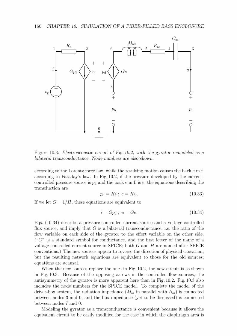
160 CHAPTER 10. SIMULATION OF A FIBER-FILLED BASS ENCLOSURE
f
f
f
fsss
JJJJ
JJ6
JJJJ
JJ
?6 ?
0
1 2 3456
7
GeGpd
vg
i u
Cas
RasMadRe
−
pf
+
−
pb
+
−
pd
+
−
e
+
−+
Figure 10.3: Electroacoustic circuit of Fig. 10.2, with the gyrator remodeled as abilateral transconductance. Node numbers are also shown.
according to the Lorentz force law, while the resulting motion causes the back e.m.f.according to Faraday’s law. In Fig. 10.2, if the pressure developed by the current-controlled pressure source is pd and the back e.m.f. is e, the equations describing thetransduction are
pd = Hi ; e = Hu. (10.33)
If we let G = 1/H, these equations are equivalent to
i = Gpd ; u = Ge. (10.34)
Eqs. (10.34) describe a pressure-controlled current source and a voltage-controlledflux source, and imply that G is a bilateral transconductance, i.e. the ratio of theflow variable on each side of the gyrator to the effort variable on the other side.(“G” is a standard symbol for conductance, and the first letter of the name of avoltage-controlled current source in SPICE; both G and H are named after SPICEconventions.) The new sources appear to reverse the direction of physical causation,but the resulting network equations are equivalent to those for the old sources;equations are acausal.
When the new sources replace the ones in Fig. 10.2, the new circuit is as shownin Fig. 10.3. Because of the opposing arrows in the controlled flow sources, theantisymmetry of the gyrator is more apparent here than in Fig. 10.2. Fig. 10.3 alsoincludes the node numbers for the SPICE model. To complete the model of thedriver-box system, the radiation impedance (Mar in parallel with Rar) is connectedbetween nodes 3 and 0, and the box impedance (yet to be discussed) is connectedbetween nodes 7 and 0.
Modeling the gyrator as a transconductance is convenient because it allows theequivalent circuit to be easily modified for the case in which the diaphragm area is

10.1. THE MOVING-COIL DRIVER 161
shared between several volume elements in the box; in the following discussion it isshown that because G is proportional to S, the transconductance is shared betweenthe volume elements in the same fractions as the diaphragm area.
Using Eq. (10.13), we may write G in terms of the Bl product as
G =1H
=SBl
. (10.35)
When the box is modeled as a finite-difference equivalent circuit, each of the volumeelements adjacent to the diaphragm covers part of the diaphragm area. Denotingthe partial areas by Sj, where j = 1, 2, . . . , n, we have
S =∑
jSj. (10.36)
By analogy with Eq. (10.35), let us define
Gj =Sj
Bl. (10.37)
Then dividing Eq. (10.36) by Bl gives
G =∑
jGj. (10.38)
The flux pumped out of the jth volume element adjacent to the diaphragm is
uj = Sj x. (10.39)
Hence multiplying Eq. (10.36) by x yields
u =∑
juj (10.40)
as expected.To model the acoustic side of the gyrator, we substitute Eq. (10.38) into the
second Eq. (10.34), obtainingu =
∑
jGj e. (10.41)
This indicates that the controlled flux source in Fig. 10.3 must be replaced by nsources, with the jth source feeding a flux Gj e into node 6.
Modeling the electrical side is more difficult because the current is no longercontrolled by a single pressure drop on the acoustic side. But we know that theaverage excess pressure on the back of the driver is pb. Let us define the areafractions as
aj =Sj
S; j = 1, 2, . . . , n (10.42)
so that Eq. (10.37) can be rewritten
Gj = aj G. (10.43)
If pbj denotes the average excess pressure on the back of the jth area element (whosearea is Sj), the area-weighted average is
pb =∑
jaj pbj. (10.44)

162 CHAPTER 10. SIMULATION OF A FIBER-FILLED BASS ENCLOSURE
Applying Kirchhoff’s pressure law to the right-hand mesh in Fig. 10.3, we have
pd = pf +1
Cas
∫
u dt + Rasu + Madu− pb. (10.45)
Substituting from Eq. (10.44) and multiplying through by G gives
Gpd = G[
pf +1
Cas
∫
u dt + Rasu + Madu]
−G∑
jaj pbj. (10.46)
The left-hand side is just i (from the circuit or from Eqs. (10.34)). In the first termon the right, we substitute for G from Eq. (10.38) and take the bracketed expressioninside the resulting summation. In the last term on the right, we take G inside thesummation and substitute from Eq. (10.43). The result may be written
i =∑
jGj pdj (10.47)
wherepdj = pf +
1Cas
∫
u dt + Rasu + Madu− pbj. (10.48)
Eqs. (10.47) and (10.48), together with the earlier Eq. (10.41) and the electricalcomponents of the driver, are modeled by the circuit of Fig. 10.4, in which we taken = 3 for the purpose of illustration. Because the back e.m.f. e is simply the voltageat node 2 relative to ground, it is written “in the node” to save space in the diagram.The developed pressures pd1 to pd3 cannot be similarly treated and must be shownas separate pressure drops. On the acoustic side of the circuit, grounded terminalsare included to facilitate the labeling of pressures. In the equivalent circuit of theinterior of the box (see next heading), the number of ground connections will begreater than the number shown in Fig. 10.4.
In summary, if the diaphragm area is shared among several volume elements, theequivalent circuit is modified as follows:
• the transconductance is partitioned in the same proportions as the diaphragmarea;
• The ratio of the jth partial flux to the common back e.m.f., and of the jth partialcurrent to the jth developed pressure, is the jth partial transconductance.
These changes are quite intuitive, especially when it is remembered that the to-tal developed pressure is a weighted average of the individual developed pressures:at low frequencies, these developed pressures are nearly equal, so that the partialtransconductance may be understood as the ratio of the partial flow on one sideof the transducer to the common effort on the other side, for both directions oftransduction.
10.2 The interior of the box
To avoid consuming unreasonable amounts of CPU time during experiments, theequivalent circuits constructed in this chapter will model the interior of the box asa two-dimensional network, with volume elements extending across the full width

10.2. THE INTERIOR OF THE BOX 163
f+
pb1
−f
f+
pb2
−f
f+
pb3
−f
f+
pf
−fs s s s s s s
s s sRe Ras
+−vg
Mad
Cas
SSSS
6
+
pd1
−G1e
SSSS
6
+
pd2
−G2e
SSSS
6
+
pd3
−G3e
SSSS
?
G1pd1
SSSS
?
G2pd2
SSSS
?
G3pd3
6i ?u
e
0
1 2 3456
7 8 9
Figure 10.4: Electroacoustic circuit of a moving-coil driver whose diaphragm areais shared between n volume elements, for n = 3. The back e.m.f. is written “in thenode”.
of the box. This is a reasonable approximation not only because the width is thesmallest overall dimension in the given examples, but also because the driver-boxgeometry is symmetrical in the width direction, so that the fundamental left-rightresonance of the box, unlike the fundamental vertical and front-back modes, cannotbe excited. Thus the effective element size in the left-right direction is half the overallwidth, whereas the element sizes in the other two directions (delx and dely) canbe made arbitrarily small.
The FDEC components may be calculated from the formulae in Chapters 6and 7, in which hu∆u and hv∆v are replaced by ∆x and ∆y respectively, and hw∆wis replaced by width, which will be abbreviated “w” in the following discussion.
When these substitutions are made in Eq. (6.38), the undamped compliance el-ement is found to be
∆C =w ∆x ∆y
γP0. (10.49)
The damped compliance element is ∆Ca in parallel with the series combination of∆Rth and ∆Cth. From Eqs. (7.82) and (7.85),
∆Ca =(1− f) w ∆x ∆y
γP0= (1− f) ∆C , (10.50)
whence Eqs. (7.116) and (7.117) may be used without modification to find ∆Rth and

164 CHAPTER 10. SIMULATION OF A FIBER-FILLED BASS ENCLOSURE
∆Cth. In the circuit diagram, the combination of ∆Ca, ∆Rth and ∆Cth will be giventhe symbol “XC” (in SPICE, the name of a subcircuit instance begins with “X”).
The undamped inertance elements, given in general orthogonal coordinates byEqs. (6.39) to (6.44), reduce to two cases:
∆Mx =ρo∆xw ∆y
(10.51)
∆My =ρo∆yw ∆x
. (10.52)
The boundary inertance element between the jth segment of the diaphragm areaand the adjacent compliance element has length ∆x/2 and area Sj, so its inertancemay be estimated as
∆M j =ρo∆x/2
Sj. (10.53)
The damped inertance element in the x direction is ∆Mxa in series with the parallelcombination of ∆Rx and ∆Mxf . From Eqs. (7.28) to (7.30), we obtain the values
∆Mxa =ρo∆x
(1− f) w ∆y=
∆Mx
1− f(10.54)
∆Rx =λ ∆x
(1− f) w ∆y=
λ ∆Mxa
ρo(10.55)
∆Mxf =fρf∆x
(1− f)2w ∆y=
fρf∆Mxa
(1− f) ρo. (10.56)
The corresponding components for the y direction are
∆Mya =ρo∆y
(1− f) w ∆x=
∆My
1− f(10.57)
∆Ry =λ ∆y
(1− f) w ∆x=
λ ∆Mya
ρo(10.58)
∆Myf =fρf∆y
(1− f)2w ∆x=
fρf∆Mya
(1− f) ρo. (10.59)
The subcircuits representing the damped inertance elements will be called XMx forthe x direction and XMy for the y direction. In the x direction there is also a groupof elements, denoted by XMb, which straddle the boundary between the undampedand damped regions. Each of these elements comprises an undamped inertance inseries with a damped inertance, each inertance being of length ∆x/2 instead of∆x. Hence XMb comprises an inertance (∆Mx + ∆Mxa)/2 in series with the parallelcombination of ∆Rx/2 and ∆Mxf/2.
With the above definitions of the components and subcircuits, the equivalent cir-cuit of the interior of the box is as shown in Fig. 10.5. For the purpose of illustrationit is assumed that the diaphragm area is shared among three volume elements (asin Fig. 10.4), that the clear region behind the driver is two elements deep, and thatthe fiber-filled region is three elements deep and five elements high; these dimen-sions differ from those of the models constructed and analyzed later in this chapter.Where a compliance element is to be connected between a node and ground, the

10.2. THE INTERIOR OF THE BOX 165
- y
?x
7 8 9e e e ∆M1 ∆M2 ∆M3
∆C ∆C ∆C
∆C ∆C ∆C
XC XC XC XC XC
XC XC XC XC XC
XC XC XC XC XC
∆Mx ∆Mx ∆Mx
∆My ∆My
∆My ∆My
XMb XMb XMb
XMx XMx XMx XMx XMx
XMx XMx XMx XMx XMx
XMy XMy XMy XMy
XMy XMy XMy XMy
XMy XMy XMy XMy
Figure 10.5: Two-dimensional finite-difference equivalent circuit for the inte-rior of the box in Fig. 10.1, with clear = 2 ∆x, depth = 5 ∆x, D = 3 ∆x andheight = 5 ∆x. Coordinate directions are indicated by the labeled axes. Rectangu-lar blocks represent lossy mass elements; the “XMb” elements straddle the boundarybetween the clear and fiber-filled regions. “∆C” denotes an undamped complianceelement and “XC” a damped compliance element; when either of these symbolsappears at a node, the corresponding element is connected between that node andground. Subcircuit names begin with “X”. The node numbers at the top indicatewhere this circuit should be connected to that of Fig. 10.4. As explained in the text,boundary elements ∆M1 to ∆M3 may be combined in parallel and added to Mad inFig. 10.4, in which case the nodes connected to the top three “∆C” elements will berenumbered 7, 8 and 9.
166 CHAPTER 10. SIMULATION OF A FIBER-FILLED BASS ENCLOSURE
compliance symbol is written “in the node”. This convention, when combined withthe small number of elements, gives a clear and uncluttered diagram. It also explainswhy no ground connections are visible.
The equivalent circuit of the driver-box combination can be simplified slightly bycomparing the pressure drops across the inertance elements adjacent to the driver.The pressure difference across ∆M j is
∆M juj =ρo∆x/2
Sj
Sj uS
= Mab u (10.60)
where
Mab =ρo∆x/2
S. (10.61)
In words, the pressure drop across each ∆M j is the same as that which wouldresult from the entire flux u flowing through the inertance Mab. Hence the sumsof voltage drops around the acoustic mesh of Fig. 10.4 will be preserved if we omiteach ∆M j and lump Mab in series with Mad. The inertance Mab may be recognizedas the parallel combination of all the ∆M j elements or as an inertance of length∆x/2 whose cross-sectional area is the diaphragm area. In effect, Mab is an air loadbehind the driver (“b” for “back” or “behind”) and is added to Mad in order tocompensate for the omission of the first layer of inertance in the finite-differenceequivalent circuit of the box interior.
10.3 Description of modeling programs
The model-building program box.c (listed in Section B.9) converts the parametersof the driver and box into an equivalent circuit specification to be processed bySPICE. Hence some familiarity with SPICE is assumed in the following description.
The model-builder uses the #define preprocessor command to specify the di-mensions of the box, the parameters of the driver and fiberglass filling, the frequencyrange for the simulation, and the desired volume element size. The actual elementdimensions are called delx in the x direction (horizontally towards the back of thebox) and dely in the y direction (vertically), and are computed subject to the re-striction that depth and height must be multiples of delx and dely respectively.The driver parameters are taken from a locally available catalog [1] and the fiberglassspecifications are the same as those used by Leach [30].
From the element sizes and box dimensions, the model-builder must computethe number of volume elements in each coordinate direction and write the circuitdefinition with the appropriate node numbers. The circuit definition is written to thefile “cct” and the SPICE command script for analyzing the circuit is written to thefile “go”. When SPICE is invoked, the files cct and go are sourced either manuallyor by the .spiceinit file. The half-space frequency response of the speaker isgraphed on-screen, and the points of the graph are simultaneously written to a file;the name of this output file is given as a command-line argument to the programbox.c, which copies it into the script go.
To facilitate comparison of frequency responses, the program “sp2tex.c” (listedin Section B.11) turns the SPICE output files into graphs which can be viewed on-screen or imported into documents. The graph-drawing program accepts one or twoinput files, allowing two frequency responses to be superimposed on one graph.

10.3. DESCRIPTION OF MODELING PROGRAMS 167
10.3.1 Command-line options
In addition to the name of the SPICE output file, the model-building programaccepts optional command-line switches indicating that some components are tobe omitted from each equivalent-circuit cell (for the command-line syntax, see thelisting in Section B.9). With no switches, box.c does a “full simulation”; that is, ituses the full equivalent circuits of Figs. 7.1 and 7.2. The following mutually-exclusiveswitches cause certain components to be omitted from the mass elements (Fig. 7.1)in both the x and y directions:
free (-f) : Resistance to air motion is ignored; ∆Mua and ∆Ru areshorted out (valid at very high frequencies);
stiff (-s) : The fiber does not move; ∆Muf is omitted (valid at suffi-ciently high frequencies);
unison (-u) : The fiber moves with the air; ∆Ru is omitted (valid atvery low frequencies).
Another three mutually-exclusive switches indicate that certain components are tobe omitted from the compliance elements (Fig. 7.2):
adiab (-a) : Compression of the air is adiabatic; ∆Cth and ∆Rth areomitted (valid at very high frequencies);
nearad (-n) : Compression is near-adiabatic; ∆Cth is shorted out (validat sufficiently high frequencies);
equil (-e) : Thermal equilibrium; ∆Rth is shorted out (valid at suffi-ciently low frequencies).
If the following switch is present, it overrides all others:
lumped (-l) : The volume of the box is modeled as a lumped com-pliance and the fiber is ignored; this gives the classical equivalent-circuit model.
If the free and adiab switches are used together, they give the so-called undampedcondition. This condition is equivalent to removing the fiber, except that the vol-umes and cross-sectional areas of the elements are multiplied by (1− f). (The useof fiber-reduced areas ensures that the free, adiab and undamped conditions areexact high-frequency limits of the full simulation. If the full areas and volumes aredesired, the filling factor should be set to a very small value.) In the following text,the names of most switches will be printed consistently in bold type; the exceptionsare “lumped” and “undamped”, which are more self-explanatory than the others.
The model-builder makes extensive use of SPICE subcircuits for the inertanceand compliance elements, so that the node-numbering code is not affected by theomission of selected components from the FDEC elements. In the subcircuits, everyopportunity is taken to lump series or parallel components so as to minimize thenumbers of components and nodes.

168 CHAPTER 10. SIMULATION OF A FIBER-FILLED BASS ENCLOSURE
10.3.2 Circuit modifications required by SPICE
A well-known feature of SPICE, which prevents many errors in the analysis of non-linear electronic circuits, is that every AC analysis is automatically preceded by aDC operating-point analysis. This has two consequences which are inconvenient forpresent purposes. First, every node must have a finite-resistance DC path to groundin order to avoid a singular-matrix error. If part of the circuit “floats”, every nodalvoltage in the floating section contains an arbitrary constant. Thus the solution isnot unique, wherefore the system equations must have a singular coefficient matrix.Second, every loop must have a non-zero DC loop resistance; otherwise the loopcurrent is indeterminate and adds an arbitrary constant to every branch current inthe loop.
Unless the nearad approximation is used, the compliance elements do not pro-vide a DC path to ground, so that nodes 4 to 7 in Fig. 10.3 are left floating. Tocorrect this, Cas is bypassed by a large resistance Rleak, whose value is chosen (some-what arbitrarily) so that RleakCas = 1000 seconds. The long time constant ensuresthat the leakage resistor has negligible effect at audio frequencies. The added resis-tor provides a DC path from ground to every node in the FDEC model of the boxinterior, via the FDEC inertance elements. It does not increase the node count andtherefore does not represent a significant computational penalty.
The requirement of non-zero loop resistances is a more serious problem becausethe inertance elements form an array of loops and, unless the stiff approximation isused, every inertance element is a short circuit for DC. To remove the shorted loops,a small resistance must be connected in series with each of the inertance elementsin either the x or the y direction. Program “box.c” chooses the x direction; hence,in Fig. 10.5, ∆Mx must be replaced by a subcircuit, and the subcircuit XMx mustbe modified. The series resistance is denoted by ∆Rxs and its value is chosen sothat ∆Mx/∆Rxs = 1000 seconds. Unfortunately the added resistances substantiallyincrease the node count, wasting storage space and CPU time. (For the sake ofconsistency, and to ensure that the stiff approximation is an exact high-frequencylimit of the full simulation, ∆Rxs is included in the stiff approximation, but it islumped with ∆Rx so as not to increase the node count.)
10.3.3 Program limitations
The two programs used in the present chapter are research prototypes only. Threelimitations of the model-building program should be noted here:
• As explained in Section 10.2, the model of the box interior is two-dimensional.If it were extended to three dimensions, subcircuits would be required forthe undamped and damped inertance elements in the z direction, and thefor-loops for writing out the compliance and inertance elements would benested three-deep. The avoidance of zero-resistance loops would require smallresistances in series with the inertance elements in two of the three coordinatedirections.
• The area of the diaphragm is assumed to be divided equally between thevolume elements immediately behind the driver. In effect, this assumes thatthe driver area is uniformly distributed vertically, whereas the two-dimensionalapproximation assumes that the area is uniformly distributed horizontally.
10.4. 10-INCH WOOFER IN 36-LITER BOX 169
Hence the errors caused by the two approximations should be of the sameorder of magnitude.
• No allowance is made for the magnet structure and the basket, which partiallyobstruct the rear of the diaphragm. Accuracy in calculating the area fractionswould be futile unless the obstructions were modeled by means of additionalacoustic elements and boundaries.
Production versions of the programs would require numerous other improvements,some of which are mentioned with the listings in Appendix B.
Clearly this is a theoretical thesis and not a software development project, sothat some limitations in the software are inevitable. At their present level of devel-opment, the programs written for this chapter illustrate the techniques developed inChapters 6 and 7, show the effect of fiber filling, allow investigation of the influenceof various fiber parameters, and—most importantly—are a quantum improvementon any analysis that neglects the spatial variation of the pressure inside the box.
10.4 10-inch woofer in 36-liter box
The listing of box.c in Section B.9 has the parameters set for a 10-inch woofer witha polypropylene cone [1]. The box dimensions are
D = width = 250 mm
depth = 300mm
height = 600mm
clear = 100mm.
These are the dimensions which are used for all simulations in this section, and forwhich Fig. 10.1 is drawn to scale. The resulting internal box volume is 36.25 liters.Unless otherwise noted, all simulations in this section use an element size of 50mm.The same element size is specified in the version of box.c listed in Section B.9. InSection B.10 is a listing of the “cct” file produced by that version of box.c for thefull simulation.
Much of the following discussion compares the results of the full simulation withthose of the various approximations, showing how the properties of the fiber affectthe frequency response. Because of the large number of graphs to be compared andthe numerous features to be explained, the discussion is long and tends to becomemired in detail. But four clear points will emerge:
• Viscosity is the dominant mechanism of damping, thermal relaxation being ofsecondary importance.
• The decision to neglect internal elastic forces in the fibers is vindicated.
• The departure from thermal equilibrium (at frequencies over a few hundredhertz) has very little effect on the response.

170 CHAPTER 10. SIMULATION OF A FIBER-FILLED BASS ENCLOSURE
• While the addition of fiber increases the output at infrasonic frequencies, itreduces the output in the bass rolloff region and does not lower the 3 dB rollofffrequency. This conclusion applies not only to the overall effect of the fiber,but also to the thermal capacity alone; the latter finding may be regarded assurprising.
Of course these conclusions apply to the system under study; that they are true forone case does not imply that they are true for all. But neither can they be lightlydismissed as “anecdotal”. Concerning the first observation, the influences of viscousand thermal damping are of different orders of magnitude. The second observation isexpected for reasons given in Subsection 7.1.1. Physical explanations for the thirdand fourth observations are offered below, with reference to the relevant graphs.A final point relevant to all observations is that the specifications of the driver-box-fiber system were partly arbitrary and partly determined by the availability ofpublished data—they were not chosen with a view to illustrating or supporting theabove conclusions, all of which emerged “after the fact”.
10.4.1 Full simulation
The frequency response predicted by the full simulation is shown in Fig. 10.6. At thelowest frequencies, for which the wavelength is much longer than the box dimensions,the curve is smooth. At the highest frequencies, for which the diaphragm accelera-tion is determined by the moving mass of the driver, the curve is again smooth. Atintermediate frequencies, the curve exhibits ripples due to the internal resonancesof the box; this feature is not predicted by classical equivalent-circuit models.
For comparison between the full simulation and the various approximations,the curve in Fig. 10.6 will be reproduced in most of the subsequent graphs in thissection. Each comparison will be accompanied by some explanation of the similar-ities and differences. The explanations may be tentative and will certainly not beexhaustive—if it were possible to explain every nuance of the graphs in words, itwould hardly have been necessary to develop the numerical techniques for comput-ing the curves—but they will at least mention the frequency range for which theapproximation should be valid, and the implications of the comparison concerningthe importance of particular fiber properties.
10.4.2 Undamped response and effect of fiber filling
Fig. 10.7 compares the undamped approximation with the full simulation. Theundamped frequency response is computed and plotted at 100 points per decade,whereas all the other frequency responses in this chapter are computed and plottedat only 50 frequencies per decade. (The “go” file for the undamped model wasmanually edited to increase the resolution of the AC analysis.)
As the undamped approximation is a high-frequency approximation, the twocurves are indistinguishable at the highest frequencies. At very low frequencies,the presence of fiber increases the heat capacity, and hence the compliance, of thebox, so that the full simulation gives more output. But this is not to say thatthe addition of fiber extends the bass response; on the contrary, the full simulationshows less output between 50 Hz and 150 Hz, because the fiber damps the motion

10.4. 10-INCH WOOFER IN 36-LITER BOX 171
Frequency (Hz)
SIL(dB)
101 102 103 1042 2 25 5 550
60
70
80
90
100
qqqqqqqqqqqqqq
qqqqqqqqqqqqqqq
qqqqqqqqqqqqqqqqqqqqqqqqqqqqqqqqqqqqqqqqqqqqqqqqqqqqqqqqqqqqqqqqqqqqqqqqqqqqqqqqqqqqqqqqqqqqqqqqqqqqqqqqqqqqqqqqqqqqqqqqqq
Figure 10.6: Half-space SIL vs. frequency for a 10-inch woofer in a 36-liter box;full simulation. The SIL (sound intensity level) is the IL at one meter, assumingisotropic radiation into half-space and constant parallel radiation resistance.
Frequency (Hz)
SIL(dB)
101 102 103 1042 2 25 5 550
60
70
80
90
100
qqqqqqqqqqqqqqqqqqqqqqqqqq
qqqqqqqqqqqqqqqqqqqqqqqqqq
qqqqqqqqqqqqqqqqqqqqqqqqqqqqqqqqqqqqqqqqqqqqqqqqqqqqqqqqqqqqqqqqqqqqqqqqqqqqqqqqqqqqqqqqqq
q
qqqqqqqqqqqqqqqqqqqqqqqqqqqqqqqqqqqq
qqqqqqqqqqqqqqqqqqqqqqqqqqqqqqqqqqqqqqqqqqqqqqqqqqqqqqqqqqqqqqqqqqqqqqqqqqqqqqqqqqqqqqqqqqqqqqqqqqqqqqqqqqqqqqqqqqqqqqqqqq
p p p p p p pp p p p p p p
p p p p p p pp p p p p p p p
p p p p p p p p p p p pp p p p p p p p p p p p p p p p p p p p p p p p p p p p p p p p p p p p p p p p p p p p p p p p p p p p p p p p p p p p p p p p p p p p p p p p p p p p p p p p p p p p p p p p p p p p p p p p p p p p p p p p p p p p p p
Figure 10.7: Undamped approximation (large dots) and full simulation (small dots).

172 CHAPTER 10. SIMULATION OF A FIBER-FILLED BASS ENCLOSURE
of the diaphragm and/or increases the effective moving mass.4 In the intermediatefrequency range, where the full simulation shows a few ripples, the undamped modelhas a series of sharp peaks and troughs. The salient features of this series are:
• The maxima and minima alternate as frequency increases;
• Each minimum is followed by a maximum at a marginally higher frequency;then there is a larger frequency gap before the next minimum.
The minima are readily explained in terms of the box impedance, i.e. the acousticimpedance seen by the diaphragm looking into the box. This impedance must bepurely imaginary (because the box interior, according to the undamped model, isnon-dissipative) and must have poles on the imaginary axis (corresponding to thenatural frequencies of the box interior when the diaphragm is held stationary). Atthe pole frequencies of the box impedance, the diaphragm cannot move, so there isno output. Hence the troughs in Fig. 10.7 theoretically extend to −∞dB. That theyappear to be of finite depth is due mainly to the finite resolution of the graph, andpartly to the small resistances which are added to the horizontal inertance elementsto avoid singular-matrix errors.
As a matter of interest, the first minimum in the undamped response is at about263Hz, corresponding to a wavelength of about 1.3m, which is slightly more thantwice the interior height of the box, and slightly less than twice the centerline-lengthof the L-shaped cavity behind the driver. So the first minimum can be understoodas the half-wave resonance.
The peaks in the undamped frequency response occur not at the zeros of thebox impedance, but at the frequencies for which the box reactance cancels the netreactance that appears in series with it on the acoustic side of the equivalent circuit.At the frequencies under discussion, the dominant reactance in series with the boxis that due to the moving mass of the driver, which is inductive, so that the boxreactance at the peak frequencies must be capacitive. Now the box reactance iscapacitive at frequencies just above the pole frequencies (because the complianceof every region increases with frequency) and inductive at frequencies just below.5
This observation alone explains why, as frequency increases, a maximum followsa minimum more closely than it is followed by the next minimum. The effect isexaggerated by the generally low impedance of the box compared with that of themoving mass of the driver; only near the poles does the box reactance become largeenough (in absolute value) to cancel that of the moving mass. Hence the minimaand maxima in Fig. 10.7 occur in closely-spaced pairs, with each pair correspondingto one resonant mode of the box. (Between 500Hz and 700 Hz are two resonanceswhich are barely resolved by the graph; the points at 83.5 dB and 94 dB belong tothe first resonance, while those at 77 dB and 92.5 dB belong to the second.)
Chapter 1 mentioned the work of Sakai et al. [47], who combined a finite-elementmodel of an undamped enclosure with a simple formula expressing the sound pressure
4In 1970, Barlow warned that if one uses enough fiber to approach the maximum compliance,“the absorption is excessive and there is no extension of the extreme bass” [6, p. 276].
5Of course these properties are shared by the impedance of any lumped passive L-C network,and the box interior is indeed modeled as such a network. However, because of the multipletransconductances used to model the driver, the box impedance does not appear at a single pointin the equivalent circuit, so it is not convenient to use general properties of passive L-C networksin the above discussion.
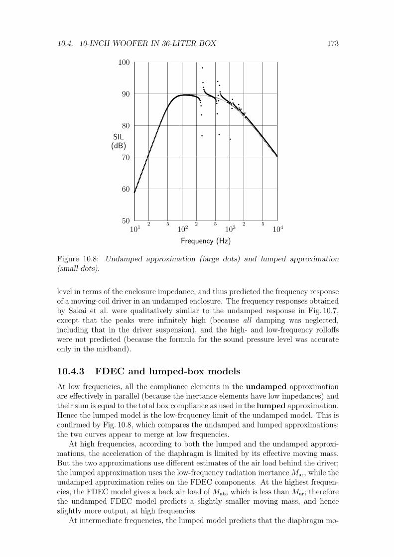
10.4. 10-INCH WOOFER IN 36-LITER BOX 173
Frequency (Hz)
SIL(dB)
101 102 103 1042 2 25 5 550
60
70
80
90
100
qqqqqqqqqqqqqqqqqqqqqqqqqq
qqqqqqqqqqqqqqqqqqqqqqqqqq
qqqqqqqqqqqqqqqqqqqqqqqqqqqqqqqqqqqqqqqqqqqqqqqqqqqqqqqqqqqqqqqqqqqqqqqqqqqqqqqqqqqqqqqqqq
q
qqqqqqqqqqqqqqqqqqqqqqqqqqqqqqqqqqqq
qqqqqqqqqqqqqqqqqqqqqqqqqqqqqqqqqqqqqqqqqqqqqqqqqqqqqqqqqqqqqqqqqqqqqqqqqqqqqqqqqqqqqqqqqqqqqqqqqqqqqqqqqqqqqqqqqqqqqqqqqq
p p p p p p pp p p p p p p
p p p p p p pp p p p p p p
p p p p p p p pp p p p p p p p p p p p p p p p p p p p p p p p p p p p p p p p p p p p p p p p p p p p p p p p p p p p p p p p p p p p p p p p p p p p p p p p p p p p p p p p p p p p p p p p p p p p p p p p p p p p p p p p p p p p p p p p p p p
Figure 10.8: Undamped approximation (large dots) and lumped approximation(small dots).
level in terms of the enclosure impedance, and thus predicted the frequency responseof a moving-coil driver in an undamped enclosure. The frequency responses obtainedby Sakai et al. were qualitatively similar to the undamped response in Fig. 10.7,except that the peaks were infinitely high (because all damping was neglected,including that in the driver suspension), and the high- and low-frequency rolloffswere not predicted (because the formula for the sound pressure level was accurateonly in the midband).
10.4.3 FDEC and lumped-box models
At low frequencies, all the compliance elements in the undamped approximationare effectively in parallel (because the inertance elements have low impedances) andtheir sum is equal to the total box compliance as used in the lumped approximation.Hence the lumped model is the low-frequency limit of the undamped model. This isconfirmed by Fig. 10.8, which compares the undamped and lumped approximations;the two curves appear to merge at low frequencies.
At high frequencies, according to both the lumped and the undamped approxi-mations, the acceleration of the diaphragm is limited by its effective moving mass.But the two approximations use different estimates of the air load behind the driver;the lumped approximation uses the low-frequency radiation inertance Mar, while theundamped approximation relies on the FDEC components. At the highest frequen-cies, the FDEC model gives a back air load of Mab, which is less than Mar; thereforethe undamped FDEC model predicts a slightly smaller moving mass, and henceslightly more output, at high frequencies.
At intermediate frequencies, the lumped model predicts that the diaphragm mo-

174 CHAPTER 10. SIMULATION OF A FIBER-FILLED BASS ENCLOSURE
Frequency (Hz)
SIL(dB)
101 102 103 1042 2 25 5 550
60
70
80
90
100
qqqqqqqqqqqqqq
qqqqqqqqqqqqqq
qqqqqqqqqqqqqqqqqqqqqqqqqqqqqqqqqqqqqqqqqqqqqqqqqqqqqqqqqqqqqqqqqqqqqqqqqqqqqqqqqqqqqqqqqqqqqqqqqqqqqqqqqqqqqqqqqqqqqqqqqqq
p p p p p p pp p p p p p p
p p p p p p pp p p p p p p p
p p p p p p p p p p p pp p p p p p p p p p p p p p p p p p p p p p p p p p p p p p p p p p p p p p p p p p p p p p p p p p p p p p p p p p p p p p p p p p p p p p p p p p p p p p p p p p p p p p p p p p p p p p p p p p p p p p p p p p p p p p
Figure 10.9: “Free” approximation, for which viscosity is neglected (large dots), andfull simulation (small dots).
tion is determined by the moving mass, giving a smooth curve, while the undampedmodel is dominated by resonances.
In the lumped model, the number of circuit nodes is fixed; but in the full simu-lation and all other approximations, the external node count6 depends only on theelement size, while the subcircuits connecting the nodes depend on the approxi-mation in use. Hence the agreement between the lumped and undamped modelsat low frequencies (for which all the compliance elements in the undamped modelcontribute to the response) is evidence that the program “box.c” calculates thecorrect compliances and connects them to the correct nodes. If the node-numberingis correct for the undamped model, it is also correct for the other finite-differencemodels.
10.4.4 Importance of viscous damping
The two approximations that neglect viscous losses but allow for thermal relaxationare the free model, which assumes that there is no resistance to air motion throughthe fiber (zero viscosity), and the unison model, which assumes that the fiber moveswith the air (infinite viscosity). The resulting frequency responses are compared withthat of the full simulation in Figs. 10.9 and 10.10, respectively. In each graph, thesubstantial difference between the two curves is due to viscous losses and shows thatviscosity is an important mechanism of damping.
In the low-frequency limit, both the free and unison models agree with the full6The “external” node count includes the terminal nodes of SPICE subcircuits, but not their
internal nodes.

10.4. 10-INCH WOOFER IN 36-LITER BOX 175
Frequency (Hz)
SIL(dB)
101 102 103 1042 2 25 5 550
60
70
80
90
100
qqqqqqqqqqqqqq
qqqqqqqqqqqqqq
qqqqqqqqqqqqqqqqqqqqqqqqqqqqqqqqqqqqqqqqqqq
qqqqqqqqqqqqqqqqqqqqqqqqqqqqqqqqqqqqqqqqqqqqqqqqqqqqqqqqqqqqqqqqqqqqqqqqqqqqqqqqp p p p p p p
p p p p p p pp p p p p p p
p p p p p p p pp p p p p p p p p p p p
p p p p p p p p p p p p p p p p p p p p p p p p p p p p p p p p p p p p p p p p p p p p p p p p p p p p p p p p p p p p p p p p p p p p p p p p p p p p p p p p p p p p p p p p p p p p p p p p p p p p p p p p p p p p p p
Figure 10.10: “Unison” approximation, for which the fiber is assumed to move withthe air (large dots), and full simulation (small dots).
simulation because the driver excursion is limited by the box compliance. They alsoagree in the high-frequency limit because the acceleration is limited by the effectivemoving mass of the driver, which at high frequencies is not greatly affected by themass of the fiber, being isolated therefrom by the compliance of the fiber-free region.Compared with the free model, the full simulation gives less output between 50Hzand 150Hz because the fiber damps the air motion and/or adds to the effectivemoving mass; at lower frequencies, the fiber still adds to the moving mass, butthis effect is swamped by the limited compliance of the box. Compared with theunison model, the full simulation gives less output around 50Hz, probably becauseit predicts greater damping of the fundamental resonance.
The unison response has larger moving masses, hence lower resonance frequen-cies, than the free model. The unison model also has a minimum-maximum pairat about 1600Hz, caused by the horizontal half-wave resonance of the fiber-free re-gion. At the boundary between the clear and fiber-filled regions there is a changein density, hence a change in impedance, hence a reflection. In the full simulation,the acoustic mass elements due to the mass of the fiber are bypassed by resis-tance elements. According to the “cct” file, the pneumatic resistivity of the fiber is1121Pa s m−2, so that it would require a 37 cm depth of fiber to produce a resistance-area product equal to ρoc. The required depth is much greater than the depth ofthe fiber-free region behind the driver. So the impedance step is small and the fullsimulation does not predict a strong reflection at the half-wave resonance of thefiber-free region.

176 CHAPTER 10. SIMULATION OF A FIBER-FILLED BASS ENCLOSURE
Frequency (Hz)
SIL(dB)
101 102 103 1042 2 25 5 550
60
70
80
90
100
qqqqqqqqqqqqqq
qqqqqqqqqqqqqqq
qqqqqqqqqqqqqqqqqqqqqqqqqqqqqqqqqqqqqqqqqqqqqqqqqqqqqqqqqqqqqqqqqqqqqqqqqqqqqqqqqqqqqqqqqqqqqqqqqqqqqqqqqqqqqqqqqqqqqqqqqq
p p p p p p pp p p p p p p
p p p p p p pp p p p p p p p
p p p p p p p p p p p pp p p p p p p p p p p p p p p p p p p p p p p p p p p p p p p p p p p p p p p p p p p p p p p p p p p p p p p p p p p p p p p p p p p p p p p p p p p p p p p p p p p p p p p p p p p p p p p p p p p p p p p p p p p p p p
Figure 10.11: “Stiff” approximation, for which the fiber is assumed stationary (largedots), and full simulation (small dots).
10.4.5 Unimportance of fiber stiffness
The third approximation affecting the inertance elements is the stiff model, whichassumes that the fiber remains stationary. In Fig. 10.11, the rigid-fiber model givesalmost the same frequency response as the full simulation. This result supports thedecision to neglect restoring forces due to the stiffness of the fibers; in the exampleconsidered, even infinite stiffness would have little effect on the result.
Initially the stiffness of the fibers was neglected because it was expected to besmall (see Subsection 7.1.1). If even infinite stiffness has little effect, we must con-clude that the movement of the fiber is not significant under the operating conditions.In the notation of Fig. 7.1, the stiff approximation assumes that most of the fluxflows in ∆Ru rather than ∆Muf , which is true at frequencies above ∆Ru/(2π∆Muf).From the values in the circuit specification file, the transition frequency is about30 Hz; at frequencies around or below this value, the mobility of the fiber (whichis taken into account by the full simulation by not by the stiff model) reduces theimpedance behind the diaphragm and allows greater output. But at such low fre-quencies the motion of the diaphragm is limited mainly by the box compliance,whose influence becomes more and more dominant as frequency decreases. Hence,in Fig. 10.11, it can be seen that the full simulation gives slightly more output overa limited frequency range (roughly 20Hz and 40 Hz), but the difference is barely re-solved by the graph (one must look for the vertical displacement between the largeand small dots).
The difference between the unison and stiff models is that ∆Mu in the unisonmodel is replaced by ∆Ru in the stiff model. As noted above, the resistivity of thefiber (represented by ∆Ru) does not cause a large impedance step at the half-wave

10.4. 10-INCH WOOFER IN 36-LITER BOX 177
Frequency (Hz)
SIL(dB)
101 102 103 1042 2 25 5 550
60
70
80
90
100
qqqqqqqqqqqqqq
qqqqqqqqqqqqqq
qqqqqqqqqqqqqqqqqqqqqqqqqqqqqqqqqqqqqqqqqqqqqqqqqqqqqqqqqqqqqqqqqqqqqqqqqqqqqqqqqqqqqqqqqqqqqqqqqqqqqqqqqqqqqqqqqqqqqqqqqqq
p p p p p p pp p p p p p p
p p p p p p pp p p p p p p p
p p p p p p p p p p p pp p p p p p p p p p p p p p p p p p p p p p p p p p p p p p p p p p p p p p p p p p p p p p p p p p p p p p p p p p p p p p p p p p p p p p p p p p p p p p p p p p p p p p p p p p p p p p p p p p p p p p p p p p p p p p
Figure 10.12: Adiabatic approximation (large dots) and full simulation (small dots).
resonance frequency of the fiber-free region, so that we should not expect to see sucha resonance in the stiff frequency response. Fig. 10.11 confirms this.
10.4.6 Secondary importance of thermal relaxation
The two approximations that neglect thermal relaxation but allow for viscous lossesare the adiab or adiabatic model (infinite thermal resistance) and the equil orthermal-equilibrium model (zero thermal resistance), whose frequency responses arecompared with that of the full simulation in Figs. 10.12 and 10.13, respectively. Inboth graphs, the difference between the two curves is due to thermal relaxation.The differences are slight; with the finite resolution of the graphs, the curves for theadiabatic and full simulations are indistinguishable for most of the frequency range,while those for the equil and full simulations cannot be distinguished at all. Tosee that the full simulation gives a slightly smoother frequency response, one mustcompare these two graphs with Fig. 10.6, in which the response of the full simulationis shown in large dots and not obscured by any other curve.
Thus the neglect of thermal relaxation has little effect on the frequency response,whereas the models that neglect viscous losses while allowing for thermal relaxation(i.e. the free and unison models, whose results appear in Figs. 10.9 and 10.10)predict very different responses from the full simulation. The contrast between thetwo classes of models is striking and indicates that viscosity, not thermal relaxation,is overwhelmingly the dominant mechanism of damping. Again it should be notedthat this conclusion is based on a particular driver-box system.
The close agreement between the equil model and the full simulation (Fig. 10.13)is easily explained. The assumption of thermal equilibrium is valid if the reactanceof ∆Cth is much greater than ∆Rth, which is the case for frequencies well below

178 CHAPTER 10. SIMULATION OF A FIBER-FILLED BASS ENCLOSURE
Frequency (Hz)
SIL(dB)
101 102 103 1042 2 25 5 550
60
70
80
90
100
qqqqqqqqqqqqqq
qqqqqqqqqqqqqqq
qqqqqqqqqqqqqqqqqqqqqqqqqqqqqqqqqqqqqqqqqqqqqqqqqqqqqqqqqqqqqqqqqqqqqqqqqqqqqqqqqqqqqqqqqqqqqqqqqqqqqqqqqqqqqqqqqqqqqqqqqq
p p p p p p pp p p p p p p
p p p p p p pp p p p p p p p
p p p p p p p p p p p pp p p p p p p p p p p p p p p p p p p p p p p p p p p p p p p p p p p p p p p p p p p p p p p p p p p p p p p p p p p p p p p p p p p p p p p p p p p p p p p p p p p p p p p p p p p p p p p p p p p p p p p p p p p p p p
Figure 10.13: Thermal-equilibrium approximation (large dots) and full simulation(small dots).
1/(2π∆Rth∆Cth). From the values in the file “cct”, the transition frequency is376Hz, so that the departure from thermal equilibrium is significant for frequen-cies of a few hundred hertz or more. At these frequencies the acceleration of thediaphragm is controlled mainly by the moving mass, so that a decrease in com-pressibility caused by thermal non-equilibrium will have little effect on the acousticoutput. If the travel of the diaphragm were compliance-limited for a range of fre-quencies extending above the range of thermal equilibrium, the responses predictedby the equil and full models would be noticeably different.
The slight difference between the responses predicted by the adiab and full sim-ulations (Fig. 10.12) is due to the heat capacity of the fiber. The full simulation givesmore output at the lowest frequencies, because the added heat capacity increases thecompliance of the box, but gives less output between 50Hz and 150Hz. One maybe tempted to ascribe the latter effect to damping of the driver-box resonance bythermal relaxation. However, as the two curves in Fig. 10.13 are indistinguishable,the equil model also gives less output than the adiabatic model in the bass rolloffregion, although neither of these models includes damping by thermal relaxation.We can explain this if we note that the equil model and the full simulation makethe air more compressible in the fiber-filled region than in the fiber-free region andtherefore predict greater airflow between the two regions, for a given diaphragmmotion, than the adiabatic model. Greater airflow increases the contribution of airload to the effective moving mass, increases viscous losses in the lower reaches of thefiber-filled region, and causes more fiber motion, increasing the contribution of thefiber to the effective moving mass. In short, the difference between the adiab andfull models in the bass rolloff region is probably due, not to the thermal effects ofthe fiber alone, but to a cascade effect in which the added heat capacity influences

10.4. 10-INCH WOOFER IN 36-LITER BOX 179
Frequency (Hz)
SIL(dB)
101 102 103 1042 2 25 5 550
60
70
80
90
100
qqqqqqqqqqqqqq
qqqqqqqqqqqqqq
qqqqqqqqqqqqqqqqqqqqqqqqqqqqqqqqqqqqqqqqqqqqqqqqqqqqqqqqqqqqqqqqqqqqqqqqqqqqqqqqqqqqqqqqqqqqqqqqqqqqqqqqqqqqqqqqqqqqqqqqqqq
pppppppppppppppppppppppppp
pppppppppppppppppppppppppp
pppppppppppppppppppppppppppppppppppppppppppppppppppppppppppppppppppppppppppppppppppppppppp
p
pppppppppppppppppppppppppppppppppppp
pppppppppppppppppppppppppppppppppppppppppppppppppppppppppppppppppppppppppppppppppppppppppppppppppppppppppppppppppppppppppp
Figure 10.14: “Free” approximation (large dots) and undamped approximation(small dots).
the mechanical inertia. Be that as it may, the example contradicts the theory thatthe heat capacity of the fiber extends the bass response.
The adiabatic and full simulations both include viscous damping, but only thelatter includes thermal relaxation. There is another pair of models in which onlyone model includes thermal relaxation while neither includes any impediment tothe flow of air through the fiber; the two models are the free and undampedapproximations, whose frequency responses are compared in Fig. 10.14. Again we seethat the model allowing for thermal relaxation (in this case, the free approximation)gives more output at infrasonic frequencies but less output between 50Hz and 150Hz.Again the latter effect may be attributed to an increase in the effective moving mass,due to the increased airflow for a given diaphragm motion. We also notice that theresonances in the free model, being only lightly damped by thermal relaxation, areeasily related to those in the undamped model.
The justification of the main findings listed in the introduction to this sectionis now complete. It remains to discuss one more approximation and investigate theeffects of element size, temperature and pressure.
10.4.7 Approximate model of thermal relaxation changesbass rolloff.
The comparison between the free and undamped models has interrupted the se-quence of approximations involving the compliance elements. The third approxima-tion in that sequence is the nearad or near-adiabatic model, which approximatesthe compliance elements as the stiff model approximates the inertance elements;

180 CHAPTER 10. SIMULATION OF A FIBER-FILLED BASS ENCLOSURE
Frequency (Hz)
SIL(dB)
101 102 103 1042 2 25 5 550
60
70
80
90
100
qqqqqqqqqqqqqqqqqqqq
qqqqqqqqqqqqqqqqqqqqqqqqqqqqq
qqqqqqqqqqqqqqqqqqqqqqqqqqqqqqqqqqqqqqqqqqqqqqqqqqqqqqqqqqqqqqqqqqqqqqqqqqqqqqqqqqqqqqqqqqqqqqqqqqqqqqp p p p p p p
p p p p p p pp p p p p p p
p p p p p p p pp p p p p p p p p p p p
p p p p p p p p p p p p p p p p p p p p p p p p p p p p p p p p p p p p p p p p p p p p p p p p p p p p p p p p p p p p p p p p p p p p p p p p p p p p p p p p p p p p p p p p p p p p p p p p p p p p p p p p p p p p p p
Figure 10.15: “Near-adiabatic” approximation, for which ∆Cth is shorted (largedots), and full simulation (small dots).
both models are valid at high frequencies and both represent the damping by meansof a single resistance. But because the nearad model affects the compliance ele-ments, it gives a much greater error at low frequencies, for which the motion of thediaphragm is compliance-limited. Hence the nearad model is unsuitable for calcula-tions involving the bass rolloff. But it is discussed here for the sake of completeness.
The nearad approximation includes ∆Rth but neglects the pressure drop across∆Cth, replacing ∆Cth with a short circuit. In physical terms, this means that thereis not enough heat conduction to make the added heat capacity significant, which isa valid assumption at sufficiently high frequencies. At low frequencies the nearadmodel becomes an absurdity because it implies that the volume element is a re-sistance instead of a compliance. If the diaphragm motion is mass-limited in themidband, the bass rolloff is first-order for a resistive box and second-order for a com-pliant box. Fig. 10.15, which compares the nearad and full simulations, confirmsthis behavior.
It must be emphasized that the near-adiabatic approximation does not simplyassume that the fiber is an infinite heatsink. The infinite-heatsink approximationsaves no computation time because it does not eliminate ∆Cth, but causes ∆Cth toassume the finite limiting value of (γ − 1)∆Ca (see Eq. (7.94)). The physical effectof an infinite heatsink is that the compression becomes isothermal as frequencyapproaches zero. Under isothermal conditions the air in the box is still a compliance,not a resistance as predicted by the nearad model.
Because the nearad model does not entirely neglect damping due to thermalconduction, it predicts a smoother frequency response, and agrees more closely withthe full simulation, than the adiab model at frequencies between 200Hz and 2 kHz.Thus the nearad model is valid over a wider frequency range, in spite of its gross
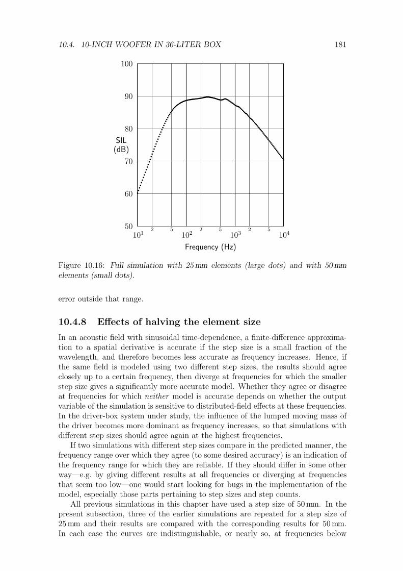
10.4. 10-INCH WOOFER IN 36-LITER BOX 181
Frequency (Hz)
SIL(dB)
101 102 103 1042 2 25 5 550
60
70
80
90
100
qqqqqqqqqqqqqq
qqqqqqqqqqqqqqq
qqqqqqqqqqqqqqqqqqqqqqqqqqqqqqqqqqqqqqqqqqqqqqqqqqqqqqqqqqqqqqqqqqqqqqqqqqqqqqqqqqqqqqqqqqqqqqqqqqqqqqqqqqqqqqqqqqqqqqqqqq
p p p p p p pp p p p p p p
p p p p p p pp p p p p p p p
p p p p p p p p p p p pp p p p p p p p p p p p p p p p p p p p p p p p p p p p p p p p p p p p p p p p p p p p p p p p p p p p p p p p p p p p p p p p p p p p p p p p p p p p p p p p p p p p p p p p p p p p p p p p p p p p p p p p p p p p p p
Figure 10.16: Full simulation with 25mm elements (large dots) and with 50mmelements (small dots).
error outside that range.
10.4.8 Effects of halving the element size
In an acoustic field with sinusoidal time-dependence, a finite-difference approxima-tion to a spatial derivative is accurate if the step size is a small fraction of thewavelength, and therefore becomes less accurate as frequency increases. Hence, ifthe same field is modeled using two different step sizes, the results should agreeclosely up to a certain frequency, then diverge at frequencies for which the smallerstep size gives a significantly more accurate model. Whether they agree or disagreeat frequencies for which neither model is accurate depends on whether the outputvariable of the simulation is sensitive to distributed-field effects at these frequencies.In the driver-box system under study, the influence of the lumped moving mass ofthe driver becomes more dominant as frequency increases, so that simulations withdifferent step sizes should agree again at the highest frequencies.
If two simulations with different step sizes compare in the predicted manner, thefrequency range over which they agree (to some desired accuracy) is an indication ofthe frequency range for which they are reliable. If they should differ in some otherway—e.g. by giving different results at all frequencies or diverging at frequenciesthat seem too low—one would start looking for bugs in the implementation of themodel, especially those parts pertaining to step sizes and step counts.
All previous simulations in this chapter have used a step size of 50mm. In thepresent subsection, three of the earlier simulations are repeated for a step size of25mm and their results are compared with the corresponding results for 50mm.In each case the curves are indistinguishable, or nearly so, at frequencies below

182 CHAPTER 10. SIMULATION OF A FIBER-FILLED BASS ENCLOSURE
Frequency (Hz)
SIL(dB)
101 102 103 1042 2 25 5 550
60
70
80
90
100
qqqqqqqqqqqqqq
qqqqqqqqqqqqqq
qqqqqqqqqqqqqqqqqqqqqqqqqqqqqqqqqqqqqqqqqqqqqqqqqqqqqqqqqqqqqqqqqqqqqqqqqqqqqqqqqqqqqqqqqqqqqqqqqqqqqqqqqqqqqqqqqqqqqqqqqqq
p p p p p p pp p p p p p p
p p p p p p pp p p p p p p
p p p p p p p p p pp p p p p p p p p p p p p p p p p p p p p p p p p p p p p p p p p p p p p p p p p p p p p p p p p p p p p p p p p p p p p p p p p p p p p p p p p p p p p p p p p p p p p p p p p p p p p p p p p p p p p p p p p p p p p p p p p
Figure 10.17: “Free” approximation with 25 mm elements (large dots) and with50mm elements (small dots).
500Hz and above 5 kHz. This is cause for confidence that the models are correctlyimplemented. (Actually the smaller step size predicts slightly more output at highfrequencies because it gives a smaller value of Mab, but the difference is too smallto show on the graphs.)
In Fig. 10.16, which compares the full simulations for the two step sizes, thecurves are indistinguishable at all frequencies. If this graph is compared withFig. 10.6, in which the 50mm full simulation is shown in large dots, it can be seenthat the curve for the 25mm full simulation is slightly rougher around 1700Hz, sug-gesting that the smaller step size detects a damped resonance which is missed bythe larger step size.
As an indication of computational complexity, the AC analysis at 50 frequenciesper decade for the full simulation with a 25 mm step size required a running time ofjust over 100 seconds on a MIPS R3000 CPU. The corresponding analysis for the50mm step size took just over 10 seconds.
Fig. 10.17 compares the free models for the two step sizes. The graph must beinspected closely to find any points of the 50 mm curve which are not obscured bythose on the other curve; such deviations occur at about 600 Hz and 1150Hz, bothin the vicinity of resonances. Comparing this graph with Fig. 10.9 shows that thecurve for the 25mm step size is slightly rougher between 2 kHz and 3 kHz.
The greatest sensitivity to step size is shown by the two undamped models,whose frequency responses are compared in Fig. 10.18. All the graphs in this thesisshow individual data points without any interpolating curves. Fig. 10.18 is onecase in which the graph would look much neater if an interpolating function wereused. Neatness would be misleading, however, because the sample frequencies wouldnot coincide with the closely-spaced maxima and minima of the response: peaks

10.4. 10-INCH WOOFER IN 36-LITER BOX 183
Frequency (Hz)
SIL(dB)
101 102 103 1042 2 25 5 550
60
70
80
90
100
qqqqqqqqqqqqqqqqqqqqqqqqqq
qqqqqqqqqqqqqqqqqqqqqqqqqq
qqqqqqqqqqqqqqqqqqqqqqqqqqqqqqqqqqqqqqqqqqqqqqqqqqqqqqqqqqqqqqqqqqqqqqqqqqqqqqqqqqqqqqqqqq
q
qqqqqqqqqqqqqqqqqqqqqqqqqqqqqqqq
q
qqqqqqqqqqqqqqqqqqqqqqqqqqqqqqq
qqqqqqqqqqqqqqqqqqqqqqqqqqqqqqqqqqqqqqqqqqqqqqqqqqqqqqqqqqqqqqqqqqqqqqqqqqqqqqqqqqqqqqqqqqqqqqppppppppppppp
pppppppppppppppppppppppppp
pppppppppppppppppppppppppppp
pppppppppppppppppppppppppppppppppppppppppppppppppppppppppppppppppppppppppppp
pppppppppppppppppppppppppppppppppppp
pppppppppppppppppppppppppppppppppppppppppppppppppppppppppppppppppppppppppppppppppppppppppppppppppppppppppppppppppppppppppp
Figure 10.18: Undamped approximation with 25mm elements (large dots) and with50mm elements (small dots).
would be too low and troughs too shallow, and some differences between resonancefrequencies would not register. It is safer to examine the scattered points.
Both responses in Fig. 10.18 are plotted at 100 frequencies per decade. Most ofthe resulting 600 points are seen to lie on a single piecewise-smooth curve; the tworesponses are indistinguishable at most sample frequencies, including all frequenciesbelow 200Hz or above 5 kHz. Between 2 kHz and 5 kHz, the smaller step size predictsa few resonances which are missed by the larger step size. In the vicinity of the lowestresonance frequency (about 265Hz), a vertical displacement can be seen between thelarge and small dots, but the slope of the response is so steep that the vertically-displaced pairs of dots still seem to lie on a common piecewise-smooth curve; hencewe may still say that the two responses are “indistinguishable, or nearly so” up to500Hz.
The double resonance in the region of 600Hz can also be interpreted by joiningalternate large and small dots with a piecewise-smooth steep curve. The first smoothsection ends with the large dot at (562Hz, 72.3 dB). The second begins with thesmall dot at (562 Hz, 93.9 dB) and ends with the small dot at (602 Hz, 77.2 dB). Thethird begins with the large dot at (616 Hz, 97.8 dB) and merges with the next gently-sloping segment. (The numbers quoted in connection with Fig. 10.18 are taken fromthe text file which was written by the SPICE “print” command and read by theplotting program “sp2tex.c”.) Notice that the frequency of 562Hz is mentionedtwice—the first apparent minimum for the 25mm step size is at the same frequencyas the subsequent apparent maximum for the 50mm step size. Thus the larger stepsize predicts a lower resonance frequency.
This observation is consistent with the one-dimensional error analysis carriedout by Arai [2, p. 20], in which a length of uniform tube was compared with its

184 CHAPTER 10. SIMULATION OF A FIBER-FILLED BASS ENCLOSURE
finite-difference equivalent circuit (an L-C ladder network). Arai found that thetotal phase lag for propagation along the pipe as predicted by the FDEC model wasgreater than the true value by a fraction
∆θθ≈ (k∆x)2
24(10.62)
where k is the wave number and ∆x is the step size (these notations are differentfrom Arai’s). Hence the fractional error in the calculated resonance frequencies (forwhich the phase lag must assume predetermined values) is
∆νν≈ − (k∆x)2
24(10.63)
where ν represents frequency. So the resonance frequencies will be underestimatedby a margin which increases with the step size.
If we use at least 2π elements per wavelength, k∆x will be not more than unityand the error will be at most one part in 24 or, conservatively, less than 5% (anequivalent result was given by Arai). The condition that k∆x ≤ 1 is satisfied forfrequencies up to c/(2π∆x), which is a little more than 1 kHz for a step size of 50mm.
To estimate the discrepancy between the resonance frequencies predicted usingtwo step sizes differing by a factor of two, we write ∆x/2 in place of ∆x in Eq. (10.63)and subtract the result from that equation. We find that the resonance frequencyfor the larger step size is lower by a fraction
(k∆x)2
32=
(
π∆x ν√8 c
)2
. (10.64)
For ∆x = 50 mm and c = 343.08 m/s, the fraction is (ν/6178Hz)2. This result comesfrom a one-dimensional plane-wave analysis. Clearly it also applies to the two- andthree-dimensional cases in Cartesian coordinates if propagation is restricted to oneof the coordinate directions. For propagation in other directions, the discrepancywill be smaller because the wavelength in the coordinate directions will be longerthan in the direction of propagation. Thus the estimated discrepancy should be anupper bound.
The highest frequency mentioned in connection with the double resonance inFig. 10.18 is 616Hz, for which the estimated discrepancy is 1%. All that can be saidfrom the data points is that the difference is less than the frequency resolution ofthe graph, which is 2.33% (for 100 points per decade). Better estimates of frequencydiscrepancies can be made by exploiting three cases in which corresponding featuresof the 50mm and 25mm curves occur at consecutive sample frequencies. The 50mmcurve has a deep dip at 1023Hz and the 25mm curve a shallower dip at 1047Hz,suggesting that the resonance frequencies are separated by a little more than 2.33%.Arai’s error estimate predicts a maximum discrepancy of 2.9%. The two curves havesimilar dips at 1122Hz and 1148 Hz; here the discrepancy is close to 2.33% whenArai’s estimate predicts 3.5%. The 50mm curve has a low peak at 1148Hz and the25mm curve a higher peak at 1174Hz, suggesting that the resonance frequenciesdiffer by a little more than 2.33%, when Arai’s estimate predicts 3.6%. In all threecases, the frequency discrepancy seems to be within the expected range.
In summary, pairs of models with different step sizes produce consistent resultswhich inspire confidence in the FDEC method and in the model-building program.
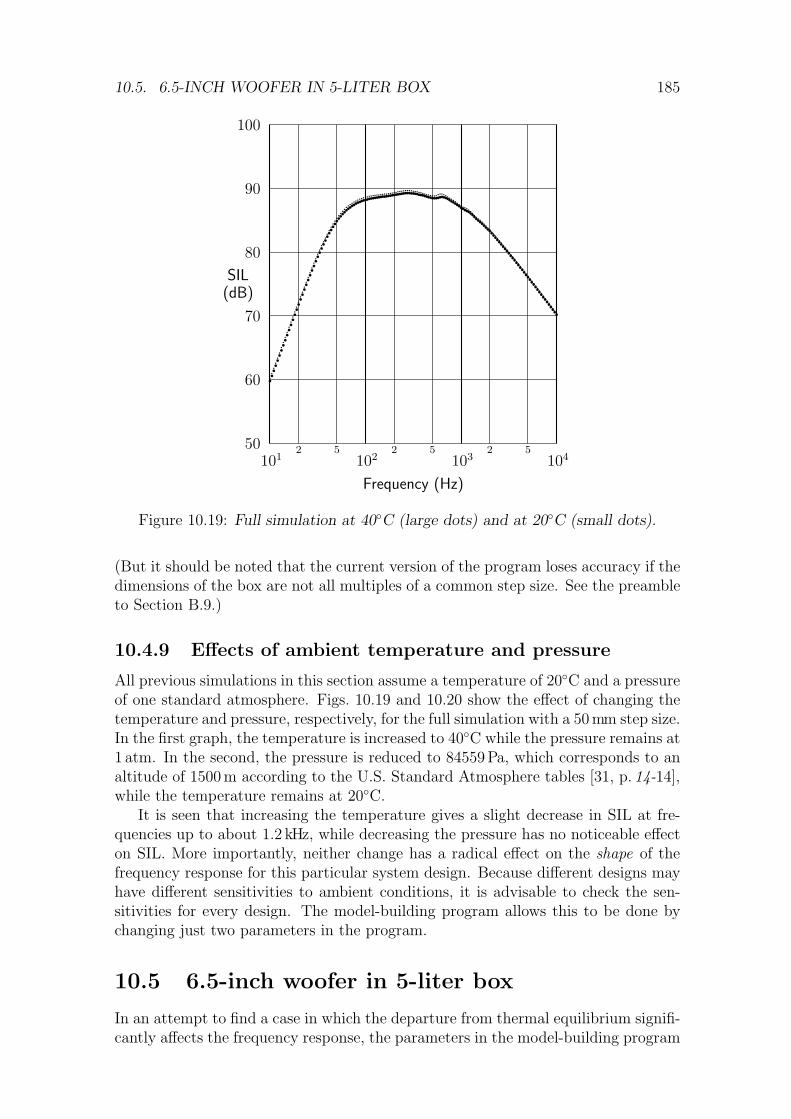
10.5. 6.5-INCH WOOFER IN 5-LITER BOX 185
Frequency (Hz)
SIL(dB)
101 102 103 1042 2 25 5 550
60
70
80
90
100
qqqqqqqqqqqqqq
qqqqqqqqqqqqqqq
qqqqqqqqqqqqqqqqqqqqqqqqqqqqqqqqqqqqqqqqqqqqqqqqqqqqqqqqqqqqqqqqqqqqqqqqqqqqqqqqqqqqqqqqqqqqqqqqqqqqqqqqqqqqqqqqqqqqqqqqqq
p p p p p p pp p p p p p p
p p p p p p pp p p p p p p p
p p p p p p p p p p p pp p p p p p p p p p p p p p p p p p p p p p p p p p p p p p p p p p p p p p p p p p p p p p p p p p p p p p p p p p p p p p p p p p p p p p p p p p p p p p p p p p p p p p p p p p p p p p p p p p p p p p p p p p p p p p
Figure 10.19: Full simulation at 40C (large dots) and at 20C (small dots).
(But it should be noted that the current version of the program loses accuracy if thedimensions of the box are not all multiples of a common step size. See the preambleto Section B.9.)
10.4.9 Effects of ambient temperature and pressure
All previous simulations in this section assume a temperature of 20C and a pressureof one standard atmosphere. Figs. 10.19 and 10.20 show the effect of changing thetemperature and pressure, respectively, for the full simulation with a 50mm step size.In the first graph, the temperature is increased to 40C while the pressure remains at1 atm. In the second, the pressure is reduced to 84559Pa, which corresponds to analtitude of 1500m according to the U.S. Standard Atmosphere tables [31, p. 14-14],while the temperature remains at 20C.
It is seen that increasing the temperature gives a slight decrease in SIL at fre-quencies up to about 1.2 kHz, while decreasing the pressure has no noticeable effecton SIL. More importantly, neither change has a radical effect on the shape of thefrequency response for this particular system design. Because different designs mayhave different sensitivities to ambient conditions, it is advisable to check the sen-sitivities for every design. The model-building program allows this to be done bychanging just two parameters in the program.
10.5 6.5-inch woofer in 5-liter box
In an attempt to find a case in which the departure from thermal equilibrium signifi-cantly affects the frequency response, the parameters in the model-building program

186 CHAPTER 10. SIMULATION OF A FIBER-FILLED BASS ENCLOSURE
Frequency (Hz)
SIL(dB)
101 102 103 1042 2 25 5 550
60
70
80
90
100
qqqqqqqqqqqqqq
qqqqqqqqqqqqqqq
qqqqqqqqqqqqqqqqqqqqqqqqqqqqqqqqqqqqqqqqqqqqqqqqqqqqqqqqqqqqqqqqqqqqqqqqqqqqqqqqqqqqqqqqqqqqqqqqqqqqqqqqqqqqqqqqqqqqqqqqqq
p p p p p p pp p p p p p p
p p p p p p pp p p p p p p p
p p p p p p p p p p p pp p p p p p p p p p p p p p p p p p p p p p p p p p p p p p p p p p p p p p p p p p p p p p p p p p p p p p p p p p p p p p p p p p p p p p p p p p p p p p p p p p p p p p p p p p p p p p p p p p p p p p p p p p p p p p
Figure 10.20: Full simulation at an altitude of 1500 meters (large dots) and at sealevel (small dots).
were reset for a 6.5-inch woofer with a carbon fiber cone [1] in a box with the fol-lowing dimensions:
D = width = height = 160mm
depth = 200mm
clear = 80mm.
The resulting internal box volume was 5.12 liters. The element size was 20mm.The frequency responses for the adiab and equil models are shown in Figs. 10.21
and 10.22, respectively. Each graph also includes the result of the full simulation.At low frequencies, as expected, the thermal-equilibrium model agrees with the fullsimulation while the adiabatic model predicts slightly less output. The interestingcomparison is in the region of the first resonance (about 800Hz). Here the adiabmodel is more accurate than the equil model, indicating a substantial departurefrom thermal equilibrium. It can be seen, albeit with some difficulty, that thethermal-equilibrium model predicts a lower resonance frequency than the other twomodels. This is because the thermal-equilibrium assumption replaces γ with γ?
o ,which reduces the speed of sound (cf. Eq. (2.40) and Subsection 7.2.3). The sameeffect can be seen, with greater difficulty, at the second resonance (about 1500Hz).
Thus the only apparent effect of the departure from thermal equilibrium is aslight shift in the frequencies of the resonant modes of the box. If this behavioris typical—as seems likely, given that the motion of the diaphragm is mass-limitedat high frequencies—the implication is that one is not likely to incur serious er-rors by assuming thermal equilibrium as recommended by Leach [30], and that theelaborate study of thermal time constants in Chapter 8 will usually have little im-pact on practical calculations. But of course this conclusion could not have been

10.5. 6.5-INCH WOOFER IN 5-LITER BOX 187
Frequency (Hz)
SIL(dB)
101 102 103 1042 2 25 5 550
60
70
80
90
100
qqqqqqqqqqqqqq
qqqqqqqqqqqqqq
qqqqqqqqqqqqqqqqqq
qqqqqqqqqqqqqqqqqqqqqqqqqqqqqqqqqqqqqqqqqqqqqqqqqqqqqqqqqqqqqqqqqqqqqqqqqqqqqqqqqqqqqqqqqqqqqqqqqqqqqqq
p p p p p p pp p p p p p p
p p p p p p pp p p p p p p
p p p p p p p pp p p p p p p p p p
p p p p p p p p p p p p p p p p p p p p p p p p p p p p p p p p p p p p p p p p p p p p p p p p p p p p p p p p p p p p p p p p p p p p p p p p p p p p p p p p p p p p p p p p p p p p p p p p p p p p p p p p
Figure 10.21: 6.5-inch driver in 5-liter box; adiabatic approximation (large dots)and full simulation (small dots).
Frequency (Hz)
SIL(dB)
101 102 103 1042 2 25 5 550
60
70
80
90
100
qqqqqqqqqqqqqq
qqqqqqqqqqqqqq
qqqqqqqqqqqqqqqqqq
qqqqqqqqqqqqqqqqqqqqqqqqqqqqqqqqqqqqqqqqqqqqqqqqqqqqqqqqqqqqqqqqqqqqqqqqqqqqqqqqqqqqqqqqqqqqqqqqqqqqqqqq
p p p p p p pp p p p p p p
p p p p p p pp p p p p p p
p p p p p p p pp p p p p p p p p p
p p p p p p p p p p p p p p p p p p p p p p p p p p p p p p p p p p p p p p p p p p p p p p p p p p p p p p p p p p p p p p p p p p p p p p p p p p p p p p p p p p p p p p p p p p p p p p p p p p p p p p p p
Figure 10.22: 6.5-inch driver in 5-liter box; thermal-equilibrium approximation(large dots) and full simulation (small dots).

188 CHAPTER 10. SIMULATION OF A FIBER-FILLED BASS ENCLOSURE
reached without first performing the work in Chapter 8. Moreover, if the character-istics of loudspeakers are not highly sensitive to thermal time constants, then theapproximations made in calculating the time constants—such as cylindrical sym-metry, perfect conduction in the fibers, and the neglect of higher-order modes—arefurther justified.
10.6 Simulations vs. experiments
Sometimes computer simulations yield information which would be difficult or im-possible to obtain from laboratory measurements. In the simulations of Sections 10.4and 10.5, the effect of each fiber property has been determined by neglecting thatproperty (by omitting the associated equivalent-circuit element) and comparing theresulting approximate simulation with the “full” simulation. In the laboratory, how-ever, it is not possible to take away the viscosity of air or the heat capacity of fiber-glass, or to hold the fibers rigid, or to suspend Fourier’s law of heat conduction,while keeping everything else constant. Indeed, given the limitations of real mate-rials, it is probably not even possible to find two types of fiber, or two gases, thatdiffer in only one relevant property.
Furthermore, computer simulations make it possible—or rather obligatory—toidealize all aspects of the system except the one(s) under study. The simulationsin this chapter show the effects of the internal air resonances acting alone, whereaslaboratory measurements might also be affected by cabinet wall vibrations, obstruc-tion by the magnet and basket, diaphragm flexure, cabinet edge diffraction, roomreflections, microphone errors, etc. Some of these influences are coupled to the in-ternal acoustic field and consequently would not cancel out in comparisons betweendamped and undamped responses. Even if the effects of cabinet wall vibrations anddiaphragm flexure can be reduced to inaudible levels, as suggested in Chapter 1 andSection 10.1, this does not imply that the effects would be unmeasurable or thatthey would not mask other phenomena under investigation.
The FDEC simulations indicate that some effects of the fiber filling are insignifi-cant compared with others; for example, it makes little difference if we assume thatthe fibers are rigid (or, equivalently, have infinite mass), or that the thermal timeconstant is infinitely long or negligibly short. Hence, in the laboratory, the effectsof these parameters would be masked by experimental error. The only parameterwhose effect would not be so masked is the pneumatic resistivity λ, which is involvedin the dominant mechanism of damping.
Thus the loudspeaker problem considered in this chapter is not a suitable testcase for an experimental validation of the FDEC method: measurements on theloudspeaker would not be accurate enough to confirm any aspect of the FDEC modelexcept the treatment of pneumatic resistivity λ. This is especially the case when werecall that the experimental results would be affected by factors not included in themodel.
However, for the purpose of understanding the mechanisms by which fiber fillingaffects the response of a loudspeaker through the damping of internal air resonances,the idealized character of the computer model used in this chapter has been anadvantage.

Chapter 11
Radiation from a circular rigidpiston
Chapter 10 is primarily concerned with an application, rather than a validation,of the FDEC method. Although the consistency of the results inspires confidence,the results were not known a priori and have not been confirmed by any sufficientlyaccurate independent method. Moreover, Chapter 10 does not use all the features ofthe FDEC model. While it thoroughly explores the circuit modifications required byfiber filling, it makes no use of curvilinear coordinates (with variable scale factors),and uses a narrow range of boundary conditions (giving a standard treatment of therigid-wall condition and an ad hoc treatment of the coupled fluxes generated by arigid diaphragm).
Hence, to conclude this study, it seems advisable to use the FDEC method tosolve a problem for which an analytical solution is known. To test the range oftechniques developed in Chapter 6, the problem should be expressed in curvilinearcoordinates and should involve a radiation condition, preferably with a range ofangles of incidence at the anechoic boundary.
11.1 Choosing the test problem
Computing the low-frequency radiation impedance on one side of a circular rigidpiston in an infinite planar baffle is a well-known problem, and is especially relevantto this thesis because its analytical solution has been used in the loudspeaker simu-lation (see Subsection 10.1.1). The low-frequency behavior of the impedance is morerelevant to the simulation in Chapter 10, and more suitable for computation by theFDEC method, than the high-frequency behavior. The problem involves two kindsboundary conditions, namely a rigid-wall condition at the baffle and an anechoicradiation condition at the free-air boundary of the simulated region.
A third boundary condition can be introduced by studying a second version ofthe problem: find the low-frequency radiation impedance on one side of an unbaffledthin disk vibrating along its axis. The modified problem is also relevant to theloudspeaker model (see Subsection 10.1.4). By symmetry, the excess pressure fieldon one side of the unbaffled disk is a mirror image of that on the other side, but hasthe opposite sign or phase. The absence of a baffle imposes continuity of pressure inthe plane of the disk, so that the equal and opposite pressures must both be zero inthat plane; that is, a zero-pressure boundary condition applies in the plane of the
189

190 CHAPTER 11. RADIATION FROM A CIRCULAR RIGID PISTON
disk.An unbaffled piston produces a net flux of zero and does not resemble a point-
source in the far field (see Subsection 6.5.4). Hence, if the anechoic-boundary ter-minations used in the baffled case are re-used in the unbaffled case, there will be re-flections from the boundary, causing an error in the computed radiation impedance.However, as the distance to the anechoic boundary is increased, the reverberantsound field in the simulated region becomes more diffuse, so that the error causedby reflection decreases. Thus we may still obtain meaningful results from the model.Moreover, because the error due to reflection is ultimately caused by the assumednormal specific acoustic impedance at the boundary, and not by the FDEC repre-sentation thereof, it depends on the distance to the outer boundary—not on thestep size. Hence, provided that the step size is sufficiently small to make reflectionthe dominant source of error, the overall error will depend more on the distance tothe outer boundary than on the step size. This prediction can be tested. For thesereasons, there is some value in proceeding with the unbaffled model even withoutcorrecting the anechoic boundary condition.
(The correction would involve finding the specific acoustic impedance in thefield of a dipole source, and using that impedance to calculate the FDEC boundaryterminations. This in turn would require repetition of much of the working in thepresent chapter, greatly lengthening the chapter for little additional benefit.)
It remains to choose a coordinate system. The geometry of the problem allows usto use a two-dimensional network if we choose an axisymmetric coordinate systemwhose axis coincides with that of the disk. For easy representation of the boundarycondition on the disk and baffle, the disk should lie in an equicoordinate surface.If we require a range of angles of incidence at the anechoic boundary, the otherequicoordinate surfaces must not be spheres centered on the disk (which give nor-mal incidence in the far field) or cones with apexes on the disk (which give tangentialincidence in the far field and extend into the near field). Using a coordinate systemother than those for which Arai formulated his method (Cartesian and cylindrical)might seem to enhance the originality of this chapter, but is also trivial in that itmerely requires specifying the scale factors. Hence, for the purpose of testing themethod, it is more useful to give a comprehensive illustration of the anechoic radia-tion condition (which was not considered by Arai) than to use an exotic coordinatesystem.1
In view of these requirements, the present chapter will use cylindrical coordinates(r, φ, z), with the disk in the plane z = 0 and coaxial with the z axis. The radiatingsurface is described by
z = 0 ; 0 ≤ r ≤ a (11.1)
while the anechoic boundaries are described by
r = b ; 0 ≤ z ≤ b (11.2)
1For more practical purposes, however, “exotic” coordinates can be useful. Geddes [18, pp. 558–61] has proposed a variety of acoustic waveguides whose walls are equicoordinate surfaces in sep-arable curvilinear orthogonal coordinate systems. The desire to analyze some of these waveguides(and others derived from non-separable coordinates) motivated the present author to develop theFDEC method in generalized orthogonal coordinates. Both infinite and truncated versions of thewaveguides could be modeled in this manner. In the present thesis, the author must be contentwith just one example in curvilinear coordinates.

11.1. CHOOSING THE TEST PROBLEM 191
andz = b ; 0 ≤ r ≤ b. (11.3)
Hence the rigid-wall or zero-pressure boundary condition must be applied at thesurface
z = 0 ; a ≤ r ≤ b. (11.4)
In other words, a is the radius of the source and b is the perpendicular distance fromthe center of the source to each of the anechoic boundaries. The angle of incidenceat the anechoic boundary ranges from zero (i.e. normal) to 45 on both the planarand cylindrical regions of the boundary, and the distance from the source to theboundary also varies, so the FDEC representation of the anechoic condition can bethoroughly tested.
11.1.1 Alternative coordinates—a digression
It should be noted that while the cylindrical coordinate system gives the most wide-ranging test of the FDEC method in solving the chosen problem, it is not ideal interms of computational efficiency or accuracy, for the chosen problem or for moregeneral problems.
Consider a general finite distributed source near the origin of a spherical coor-dinate system (R, θ, φ); here the radial coordinate is called R to distinguish it fromthe r of cylindrical coordinates. As shown in Subsection 6.5.4, the pressure field canbe written in the form
P = D(ω, R, θ, φ) U0jωρo
4πe−jkR
R(11.5)
where the R-dependence of D is negligible for large R. The angular dependenceof P is contained in the factor D. Because D approaches a function of frequencyand angular position as R →∞, the angular dependence of P does not becomemore complex as R increases. This implies that we can maintain nearly uniformaccuracy for all R by using spherical coordinates to construct the FDEC elements;while the linear dimensions of the elements in the tangential directions (θ and φdirections) increase with R, there is no loss of accuracy in the tangential finite-difference approximation, because the angular factor of P depends on the angularcoordinates and not on the associated tangential distances. In other words, there isno point in maintaining a constant linear step size in the tangential direction as theradius increases.
Hence the spherical coordinate system, or any other system which approximatesspherical coordinates at large distances from the origin, offers an advantage in com-putational efficiency: there are two tangential coordinates whose scale factors in-crease with distance from the origin, so that a finite-difference scheme in thesecoordinates has a tangential resolution that becomes coarser as radius increases.The cylindrical coordinate system, in contrast, has only one variable-scale coordi-nate; hence, if a cylindrical FDEC model is to have the same near-field resolutionas a spherical model, it will have many more elements in the far field. Cartesiancoordinates, which have no variable scale factors, require still more far-field elementsfor a given near-field resolution. So it seems that spherical coordinates will be moreefficient than cylindrical coordinates, which in turn will be more efficient than Carte-sian coordinates, for solving a general radiation problem with given accuracy usingthe FDEC method.

192 CHAPTER 11. RADIATION FROM A CIRCULAR RIGID PISTON
Of course the surface of the source may not be an equicoordinate surface inspherical coordinates, but it may be approximated by a piecewise-equicoordinatesurface in spherical (or other) coordinates, and the approximation may be madearbitrarily accurate by taking a sufficiently small step size. The appropriate sourceboundary condition can then be applied using the techniques of Section 6.5.
For the circular-rigid-piston problem, the most efficient coordinate system isprobably the oblate spheroidal system (ξ, θ, φ) used by Geddes [19, p. 453], withthe origin diameter d set equal to the source diameter. These coordinates not onlyapproximate spherical coordinates at large radii, but also give enhanced resolutionaround the edges of the disk (see Geddes’ Fig. 1), where the air motion is mostcomplex.
For present purposes, however, the choice of coordinates is driven by curiosityrather than efficiency.
11.2 The FDEC components
Following the notation of Chapter 6, let the step sizes be ∆r in the radial (r)direction and ∆z in the axial (z) direction. As the wavefront will propagate in bothdirections, we make ∆r = ∆z. Let the radius of the piston span m elements, so that
a = m∆r , (11.6)
and let the radius of the simulated region span n elements, so that
b = n∆r = n∆z = na/m. (11.7)
Thus b must be an integral multiple of a/m. Restricting b to discrete values doesnot reduce the generality of the model; b is not “given”, but merely needs to be largeenough to place the outer boundary in the far field, so that the normal impedanceat the anechoic boundary can be estimated using the point-source assumption (seeSubsections 3.3.4 and 6.5.4).
In exploiting the axial symmetry we take ∆θ = 2π, so that the volume elementsare coaxial toroids of rectangular cross-section. The coordinates at the “midpoints”(or centroidal circles) of the volume elements are
ri = (i− 12) ∆r ; i = 1, 2, . . . , n (11.8)
andzk = (k − 1
2) ∆z ; k = 1, 2, . . . , n (11.9)
Thus integer values of i and k correspond to the centers of compliance elements,while mass elements have non-integer values; for example, k is half an odd integerfor the interior axial mass elements, and i = n + 1
4 for the “truncated” radial masselements adjacent to the cylindrical boundary. The scale factor for θ is r, so thelinear increment in the θ direction is
[hθ∆θ]ik = 2πri. (11.10)
N.B.: In this section (Section 11.2), k is the step-counter in the z direction, notthe wave number.

11.2. THE FDEC COMPONENTS 193
11.2.1 Compliance and mass elements
To find the FDEC elements for the simulated region of air, we substitute the coor-dinate increments and scale factors (in terms of ri) into Eqs. (6.38) to (6.44), thensubstitute for ri from Eq. (11.8). The two steps can be shown on one line. (To pre-serve clarity of form in the algebraic expressions, the equality of ∆r and ∆z will notbe used until Section 11.3, where we consider normalizing the FDEC elements sothat the result of the simulation can be scaled for different dimensions and differentacoustic media.) Note that because the only variable scale factor depends on ri only,the values of all the interior elements will be functions of i.
The general compliance element is
∆Cik =2πri∆r∆z
ρoc2 =(2i− 1)π(∆r)2∆z
ρoc2 . (11.11)
This expression can be used even for elements adjacent to the boundaries; there areno “truncated” volume or compliance elements.
The mass elements in the radial direction are
∆M r|i+ 12 ,k =
ρo∆r2πri+ 1
2∆z
=ρo
2πi∆z(11.12)
for i = 1, 2, . . . , n− 1 ; k = 1, 2, . . . , n. This expression is valid for all but the outer-most elements, which are
12∆M r
∣
∣
∣
n+ 14 ,k
=ρo∆r
4πrn+ 14∆z
=ρo
(4n− 1) π∆z(11.13)
for k = 1, 2, . . . , n.The interior mass elements in the axial direction are
∆M z|i,k+ 12
=ρo∆z
2πri∆r=
ρo∆z(2i− 1) π(∆r)2 (11.14)
for i = 1, 2, . . . , n ; k = 1, 2, . . . , n− 1. The boundary elements are
12∆M z
∣
∣
∣
i, 34= 1
2∆M z
∣
∣
∣
i,n+ 14
=ρo∆z
4πri∆r=
ρo∆z(4i− 2) π(∆r)2 (11.15)
for i = 1, 2, . . . , n. Because the element values do not depend on k, the boundaryelements are simply half the interior elements for the corresponding values of i. Inthe case of the baffled piston, the truncated axial mass elements adjacent to the bafflecarry no flux and may be omitted. For the unbaffled piston, with its “ground-plane”boundary condition, all the truncated mass elements must be included.
11.2.2 Anechoic-boundary elements
Let R be the spherical radial coordinate and r the cylindrical radial coordinate, sothat
R2 = r2 + z2. (11.16)
In this notation, the radial specific acoustic admittance given by Eq. (3.39) becomes
yR =1
ρoc+
1jωρoR
. (11.17)

194 CHAPTER 11. RADIATION FROM A CIRCULAR RIGID PISTON
Let the angle of incidence on the anechoic boundary be α, and let the boundaryarea element be ∆S. Then the normal acoustic admittance of an anechoic surfacesegment is
∆Y = yR ∆S cos α (11.18)
(cf. Eqs. (6.86) and (6.90)).On the cylindrical part of the boundary we have
r = b∆S = 2πb∆z
cos α = b/R.
Substituting for yR, ∆S and cos α in Eq. (11.18), and introducing the subscript r toindicate that the normal to the boundary is in the r direction, we obtain
∆Y r =2πb2∆zρocR
+2πb2∆zjωρoR2 . (11.19)
Now we use the discrete values of z, introducing the subscripts b and k to indicater = b and z = zk. Substituting from Eqs. (11.16) and (11.9), with r = b = n∆z inEq. (11.16), we obtain
∆Y r|bk =1
∆Rr|bk+
1jω ∆M r|bk
(11.20)
where
∆Rr|bk =ρoc2πb2
[
n2 +(
k − 12
)2] 1
2(11.21)
∆M r|bk =ρo∆z2πb2
[
n2 +(
k − 12
)2]
. (11.22)
Thus the acoustic admittance of the kth boundary area element is that of a resistance∆Rr|bk in parallel with an inertance ∆M r|bk.
On the planar part of the boundary we have
z = b∆S = 2πr∆r
cos α = b/R.
Substituting for yR, ∆S and cos α in Eq. (11.18), and introducing the subscript z toindicate that the normal to the boundary is in the z direction, we obtain
∆Y z =2πrb ∆r
ρocR+
2πrb ∆rjωρoR2 . (11.23)
Now we use the discrete values of r, introducing the subscripts i and b to in-dicate r = ri and z = b. Substituting from Eqs. (11.16) and (11.8), and puttingz = b = n∆z everywhere, we obtain
∆Y z|ib =1
∆Rz|ib+
1jω ∆M z|ib
(11.24)

11.2. THE FDEC COMPONENTS 195
where
∆Rz|ib =ρoc
2π(∆r)2
[
1n2 +
1(i− 1/2)2
] 12
(11.25)
∆M z|ib =ρo
2π∆r
[
i− 12
n+
ni− 1
2
]
. (11.26)
Thus the acoustic admittance of the ith boundary area element is that of a resistance∆Rz|ib in parallel with an inertance ∆M z|ib.
11.2.3 Diaphragm interface
The area of the ith annular segment of the disk surface is
∆Si = 2πri∆r = 2π(i− 12)(∆r)2. (11.27)
The corresponding fraction of the total diaphragm area is
ai =∆Si
πa2 (11.28)
or, substituting from Eqs. (11.6) and (11.27),
ai =2i− 1m2 . (11.29)
Let the total flux pumped out by the diaphragm (in phasor form) be U , of whichthe ith annular segment contributes Ui. Then we have
Ui = aiU =Si
πa2 U (11.30)
for i = 1, 2, . . . ,m. Let Pi be the (phasor) excess pressure over the ith annular seg-ment, Fr the total force (i.e. the integral of excess pressure over the diaphragm area),and Pr the radiated pressure (i.e. the average excess pressure over the diaphragm).Then
Pr =1
πa2 Fr =1
πa2
m∑
i=1SiPi =
m∑
i=1
Si
πa2 Pi =m
∑
i=1aiPi. (11.31)
The ith annular segment is part of the boundary of the volume element ∆V i1,in which the central pressure is Pi1. Between the center and the boundary of thevolume element is the truncated mass element 1
2∆M z
∣
∣
∣
i, 34, so that
Pi = Pi1 + jω 12∆M z
∣
∣
∣
i, 34Ui. (11.32)
Putting12∆M z
∣
∣
∣
i, 34=
ρo ∆z/2Si
(11.33)
and substituting for Ui from Eq. (11.30) gives
Pi = Pi1 + jωMaf U (11.34)

196 CHAPTER 11. RADIATION FROM A CIRCULAR RIGID PISTON
where
Maf =ρo ∆z/2
πa2 . (11.35)
Maf may be recognized as the acoustic mass of a cylinder of length ∆z/2 and cross-sectional area πa2, or as the parallel combination of the m truncated axial masselements in front of the diaphragm (cf. Section 10.2); the subscript “f” stands for“front”. Substituting Eq. (11.34) into Eq. (11.31) yields
Pr =m
∑
i=1ai (Pi1 + jωMaf U)
=m
∑
i=1aiPi1 + jωMaf U
m∑
i=1ai
and the area fractions ai add up to unity, so that
Pr = jωMaf U +m
∑
i=1aiPi1. (11.36)
At this point we have all the equations needed to construct the equivalent circuit.However, the present form of the equations requires us to construct and solve adifferent equivalent circuit for each set of values of the parameters a, ρo and c. Aswill be shown in the next section, this limitation can be overcome by normalizingthe circuit, solving the circuit once, and denormalizing the solution for each set ofproblem parameters.
11.3 The normalized FDEC model
We begin with a comment on notation. In most parts of this thesis, maximumclarity is achieved by using the most familiar notation in each context. Inevitablythis policy causes some symbols to be reused: T can be a temperature or a period, θcan be a temperature rise or an angle, H can be a transfer resistance or a principalcurvature, and so on. Usually the different meanings of a symbol occur in disjointcontexts so that there is no risk of confusion. In this section, however, previously-defined notations mean that k usually represents a counter in the z direction, butsometimes means the wave number. So the meaning of k will be clarified at a fewpoints in the text. There are also cases in which the presence of a subscript hasan unusually radical effect, changing the type of quantity represented by a symbol.These will be noted in the appropriate places.
11.3.1 General principles; accuracy
Let the radiation impedance of the circular piston be Zar. Its area is πa2. If thisarea were a segment of a planar wavefront, its acoustic impedance would be
Za0 =ρocπa2 . (11.37)
We may regard Za0 as the “natural” unit of impedance for this problem, and hencedefine the normalized radiation impedance as
zar =Zar
Za0. (11.38)

11.3. THE NORMALIZED FDEC MODEL 197
We may also define the normalized angular frequency as
h = ka = ωa/c (11.39)
(where k is the wave number), so that a larger piston requires a lower ω for a givenh. If h 1, the piston emits approximately planar wavefronts, so that zar ≈ 1.
(Note that h with a subscript denotes a coordinate scale factor, while an un-subscripted h is the normalized angular frequency; only the latter appears in theremainder of this chapter.)
For plane waves in Cartesian coordinates, the FDEC model gives a phase er-ror of less than 5% for frequencies in the range |k∆x| < 1 (see the introduction toChapter 6). In non-Cartesian coordinates, the first derivatives of the wave functionare modulated by functions of the scale factors (see Eq. (6.35)), increasing the band-width prior to the second differentiation. Thus, for a given linear step size, we mayexpect the bandwidth over which a given accuracy is achieved (the “accuracy band-width”) to be less than for Cartesian coordinates. For non-plane waves, the wavefunction itself is modulated, so that the accuracy bandwidth should be less thanfor plane waves. Because the accuracy of the FDEC method depends on the wavefunction, the step size required for a given accuracy cannot generally be predicted,but can be estimated by studying the convergence of the solution as the step size isreduced. As the purpose of the present chapter is to test the method rather thansolve a new problem, we can use signals within the accuracy bandwidth applicableto plane waves traveling in the z direction, i.e. within the band |k∆z| < 1, not-ing that the test is made more severe by the coordinate system and the nature ofthe solution. To express this frequency band in terms of h, we put ∆z = a/m andmultiply through by m, obtaining
|ka| < m , (11.40)
i.e.|h| < m. (11.41)
Eqs. (11.38) and (11.39) can be applied to individual acoustic elements in themodel. A resistance is normalized by dividing by Za0. For a mass or compliance, weexpress the normalized impedance in terms of jh in order to obtain the normalizedcomponent value. As an example, let us normalize the radiation inertance Mar (cf.Subsection 10.1.1) and find a physical interpretation of the result. The normalizedimpedance of Mar is
jωMar
Za0= jωMar
πa2
ρoc= jh mar (11.42)
where mar is the normalized inertance, given by
mar =πaρo
Mar. (11.43)
From this we see that the natural unit of acoustic mass, i.e. the value of Mar requiredto give mar = 1, is
Ma0 =ρo
πa=
ρoaπa2 , (11.44)
which is the acoustic mass of a circular cylinder of length a and radius a. Sincethe above argument could have used any acoustic mass in place of Mar, Eq. (11.43)shows the general procedure for normalizing an inertance element.

198 CHAPTER 11. RADIATION FROM A CIRCULAR RIGID PISTON
Both the normalized radiation impedance and the normalized frequency are di-mensionless. So if we solve the radiation impedance problem for particular values ofa, ρo and c, and then plot the normalized radiation impedance vs. h, we may expectthat the resulting plot is valid for all a, ρo and c, and that we may account fordifferent values of these parameters when denormalizing the abscissa and ordinateto obtain ω and Zar. To turn this intuitive expectation into a proof, we performthe normalization of Zar by scaling all the impedances in the equivalent circuit—i.e.by normalizing the components. The normalized values of all the components willturn out to be independent of a, ρo and c, confirming that the normalized overallimpedance must also be independent of these quantities.
11.3.2 Components
In the following text, the normalized components are represented by lower-caseletters without a leading “∆”. Redundant k-subscripts (for components whose val-ues are independent of the counter k) are dropped. Non-redundant subscripts arerounded to integers because they become array indices in in the model-building pro-gram. (If k appears in a subscript or as an array index, it obviously represents acounter rather than the wave number.) The values of the components to be normal-ized are given by Eqs. (11.11) to (11.26), above.
The normalized admittance of ∆Cik is
Za0 jω∆Cik = jh ci (11.45)
where ci is the normalized compliance element and is given by
ci =2i− 1m3 . (11.46)
The notation “ci” becomes “c[i]” in the program disk.c (listed in Section B.12),which uses a one-dimensional array to store the possible compliance values.
Recalling Eqs. (11.43) and (11.44), we normalize inertance elements by multi-plying by πa/ρo. Where necessary, we also use the relations a = m∆r = m∆z andb = n∆r = n∆z. The interior radial mass element ∆M r|i+ 1
2 ,k normalizes to
mri =m2i
(11.47)
which is represented in the model-building program as mr[i]. The truncated radialmass element 1
2∆M r
∣
∣
∣
n+ 14 ,k
becomes
mrn =m
4n− 1(11.48)
which is represented in the model-building program as mr[n]. This notation isinconsistent (in the sense that mrn cannot be obtained from mri by putting i = n)but has the advantage that the truncated mass element can be stored in the samearray as the interior elements. The interior axial mass element ∆M z|i,k+ 1
2normalizes
tomzi =
m2i− 1
(11.49)

11.3. THE NORMALIZED FDEC MODEL 199
which becomes mz[i] in the model-building program. Because the truncated axialmass elements are simply half the corresponding interior elements, their normalizedvalued are not stored in an array like the truncated radial elements, but are computedas they are written to the circuit definition file. Consequently, the truncated axialmass elements in the normalized circuit diagram (Fig. 11.1) have labels beginningwith “1
2”, while the corresponding radial elements do not.To normalize the anechoic-boundary elements, the mass elements are treated as
above while the resistance elements are simply divided by Za0 (see Eq. (11.37)). Onthe cylindrical part of the boundary, ∆Rr|bk becomes
rrbk =m2
2n2
[
n2 +(
k − 12
)2] 1
2(11.50)
while ∆M r|bk becomes
mrbk =m2n2
[
n2 +(
k − 12
)2]
. (11.51)
These are represented in the model-building program as rrb[k] and mrb[k] respec-tively. On the planar part of the boundary, ∆Rz|ib becomes
rzib =m2
2
[
1n2 +
1(i− 1/2)2
] 12
(11.52)
while ∆M z|ib becomes
mzib =m2
[
i− 12
n+
ni− 1
2
]
. (11.53)
These are represented in the model-building program as rzb[i] and mzb[i] respec-tively.
The normalized value of Maf may be found by the usual scaling method (withthe substitution ∆z = a/m), or by combining the first m values of 1
2mzi in parallel(using the formula for the sum of an arithmetic progression). The result is
maf =1
2m(11.54)
which appears in the program as mf.
11.3.3 Pressure, flux, diaphragm interface
So far we have defined procedures for normalizing the radiation impedance andfrequency, and hence acoustic resistance, compliance and inertance. Because thesemethods are based on the ratio of pressure to flux, the normalized pressure andnormalized flux are only determined up to a common scale factor. But it is easy tochoose the scale factor so as to make the normalized quantities dimensionless. Theradiation impedance is
Zar =Pr
U. (11.55)
Substituting Eqs. (11.55) and (11.37) into Eq. (11.38), we obtain
zar =Pr/U
ρoc/(πa2)=
Pr/(ρoc)U/(πa2)
=Pr/(ρoc2)U/(πa2c)
(11.56)

200 CHAPTER 11. RADIATION FROM A CIRCULAR RIGID PISTON
where the last step makes the numerator and denominator dimensionless. Thus wemay write
zar =Pr
U(11.57)
where Pr and U are the normalized pressure and flux, given by
Pr =Pr
ρoc2 (11.58)
U =U
πa2c. (11.59)
These dimensionless quantities have simple physical meanings. Since ρoc2 is theadiabatic bulk modulus, Pr is the phasor form of the fractional increase in density.Let Q denote the (phasor) average velocity over the diaphragm area, so that
Q =U
πa2 . (11.60)
Then the normalized flux can be written
U =Qc
(11.61)
showing that U is the average velocity expressed as a fraction of the velocity ofsound. These physical interpretations indicate that, if the assumptions of smallcompressions and small oscillations hold, we will have Pr 1 and U 1.
The normalized pressure and flux are useful in the normalization of the equationsdescribing the diaphragm interface. When the left-hand equality in Eq. (11.30) isdivided through by πa2c, it becomes
Ui = aiU (11.62)
confirming the obvious fact that the normalized fluxes, like the unnormalized fluxes,divide in proportion to the area fractions. A more interesting conclusion is obtainedby dividing Eq. (11.36) through by ρoc2. The result can be expressed in the form
Pr
ρoc2 =jωMaf Uρoc/(πa2)
+m
∑
i=1
[
aiPi1
ρoc2
]
(11.63)
and then rewritten term-by-term to obtain
Pr = jhmaf U +m
∑
i=1aiPi1 (11.64)
which has the same form as Eq. (11.36) but involves only normalized quantities.Recalling the comment made after Eq. (11.36), we now have all the equations
needed to draw the normalized finite-difference equivalent circuit; this is shown inFig. 11.1. The coordinate directions (but not the location of the origin) are indicatedby the axes at lower right. As in Fig. 10.5 in the previous chapter, a compliancebetween a node and ground is indicated by writing the compliance “in the node”.Eqs. (11.62) and (11.64), which describe the diaphragm interface, are implemented

11.3. THE NORMALIZED FDEC MODEL 201
r
r
r
rr
r
rr
r
rr
r
rr
r r
r
r r
r
r r
r
r r
r
r r
r
r rr
c1
c1
c1
c1
c1
c2
c2
c2
c2
c2
c3
c3
c3
c3
c3
c4
c4
c4
c4
c4
c5
c5
c5
c5
c5
mr1
mr1
mr1
mr1
mr1
mr2
mr2
mr2
mr2
mr2
mr3
mr3
mr3
mr3
mr3
mr4
mr4
mr4
mr4
mr4
mr5
mr5
mr5
mr5
mr5
mz1
mz1
mz1
mz1
mz2
mz2
mz2
mz2
mz3
mz3
mz3
mz3
mz4
mz4
mz4
mz4
mz5
mz5
mz5
mz5
mz12
mz22
mz32
mz42
mz52
mz42
mz52
rrb1
rrb2
rrb3
rrb4
rrb5
mrb1
mrb2
mrb3
mrb4
mrb5
mz1b mz2b mz3b mz4b mz5brz1b rz2b rz3b rz4b rz5b
JJ JJ6
−
+
JJ JJ6
−
+
JJ JJ6
−
+
r rp11 p21 p31
a1u a2u a3u
QQQQ
QQQQ
QQQQ
a1p11 a2p21 a3p31 maf JJ
JJ6
−
+pr
u
r
m+2 m+1+n
1 2 m = 3 m+1
- r
6z
Figure 11.1: Normalized FDEC model of a circular rigid piston, with or withoutan infinite planar baffle, in cylindrical coordinates (r, φ, z), with m = 3 and n = 5(see text). Selected nodes are numbered in terms of m and n. The truncated axialmass elements 1
2mzi are present only in the unbaffled case. The anechoic-boundaryadmittance elements are strictly valid only in the baffled case.

202 CHAPTER 11. RADIATION FROM A CIRCULAR RIGID PISTON
by the array of coupled controlled sources at the bottom of the diagram. Theflux source u is used only for the AC analyses (Section 11.4); it is replaced by araised-cosine pressure source for the subsequent transient analysis (Section 11.5).The diagram shows both the baffled and unbaffled versions of the problem; dottedlines indicate that the truncated axial mass elements 1
2mzi are present only in theunbaffled case. The anechoic-boundary admittance elements (parallel “R-L” combi-nations) are calculated for a point-source and are accurate only in the baffled case.The error caused by the false point-source assumption will be seen in Section 11.4.
A review of the notation used in Fig. 11.1 may help avoid confusion. A sub-scripted r is an anechoic-boundary resistance element, while r without a subscript(or in a subscript) is the radial coordinate. A subscripted m is a mass element (areal number), while an unsubscripted m is the number of elements spanned by theradius of the diaphragm (an integer). A subscripted a is an area fraction, while anunsubscripted a (used in the text but not in the diagram) is the radius of the di-aphragm. The values of the truncated axial mass elements are given in terms of thecorresponding interior elements (hence the factor 1
2); the truncated radial elementsare labeled independently. Finally, whereas the text discusses phasor quantities (e.g.Pr and U), the diagram shows the corresponding time-dependent quantities (pr andu) because the mass elements are shown as real inductances rather than imaginaryimpedances.
A few notes on the node-numbering scheme are also in order. For illustrativepurposes Fig. 11.1 is drawn for m = 3 and n = 5, although actual simulations de-scribed in this chapter use larger values of m and n. To facilitate comparison withthe model-building program disk.c, the diagram shows some selected node num-bers in terms of m and n. As always in SPICE, ground is node zero. Numberingof non-grounded nodes begins with the diaphragm interface, and then proceeds tothe centers of the volume elements. The node number increases by one for eachincrement in i (or ri). The diagram suggests that there are n + 1 non-groundednodes in each row (i.e. in each constant-z plane), so that incrementing k (or zk)should increases the node number by n + 1. However, the SPICE model uses a sub-circuit for each combination of a truncated mass element and an anechoic-boundaryimpedance, so that the outermost non-grounded nodes in Fig. 11.1 (which are notcenters of volume elements) become internal nodes in the subcircuits and do notcontribute to the global node count. Thus the node number increases by n for eachincrement in k. Combining these rules, we find that the node number for the centerof the i, kth volume element is m + 1 + (k−1)n + i.
A listing of the model-building program disk.c, together with a discussion ofimplementation issues specific to SPICE, may be found in Section B.12. Followingthis, in Section B.13, is a listing of the circuit-definition file for the unbaffled diskwith m = 3 and n = 5; this is the file created by disk.c to describe the circuit inFig. 11.1. The values of m and n are passed to disk.c by command-line parameters.A third parameter selects between an AC analysis of a baffled disk, an AC analysisof an unbaffled disk, and a transient analysis of a baffled disk. The fourth and finalparameter is the base name of the output files to be written by SPICE.
As in Chapter 10, the model-building program also creates a SPICE commandfile. The base name of the SPICE output files is obviously copied to this file. Someother features of the command file are explained in the following two sections.

11.4. AC ANALYSIS: RADIATION IMPEDANCE 203
11.4 AC analysis: radiation impedance
As in Subsection 10.1.1, the radiation impedance Zar will be represented as an acous-tic resistance Rar in parallel with an acoustic mass Mar. The normalized values ofthese three quantities are denoted by zar, rar and mar, respectively. By allowing rar
and mar to be frequency-dependent, this representation can be extended to arbitrar-ily high frequencies, although the calculation of the impedance itself is reliable onlyfor normalized frequencies in the range |h| < m.
It remains to show how rar and mar are calculated using SPICE. Using a nota-tion similar to that of SPICE expressions, let P (`) denote the (phasor) normalizedpressure at node `. Then, with reference to Fig. 11.1, the radiation admittance canbe written
UP (m + 1)
=1zar
=1rar
+1
jhmar. (11.65)
Taking real parts and solving for rar, we obtain
rar =1
Re
U/P (m + 1) . (11.66)
We could similarly obtain mar by taking imaginary parts, but the resulting expres-sion would depend on h, which in SPICE would be represented as 2*pi*frequency.A simpler expression can be obtained by referring again to Fig. 11.1 and noting that
P (1)U
=1
jhmaf. (11.67)
Multiplying Eqs. (11.65) and (11.67), taking real parts and solving for mar, we obtain
mar =maf
Re
P (1)/P (m + 1) . (11.68)
Eqs. (11.66) and (11.68) were used in the SPICE command files; the formerequation was simplified by choosing U = 1. In the baffled case, the output generatedby the SPICE “print” command was processed by the program taba.c to produceTable 11.1. In the unbaffled case, the SPICE output was processed by the programtabu.c to produce Table 11.2. (The two programs, which are quite similar, arelisted in Section B.14.)
The variable f in the first column of Table 11.1 is the frequency variable used bySPICE, while the second column is the normalized radian frequency h; as h = 2πf,we can interpret f as the normalized cycle frequency. In both the resistance sectionand the inertance section, the frequency increases as we read down the page; hencethe top line of each section should be compared with the low-frequency limit givenby Beranek (see Eqs. (10.1) and (10.2)). For the reader’s convenience, these limitshave been normalized and printed in the headings of the two sections of the table.
The third, fourth and fifth columns use the same n/m ratio (or b/a ratio), butm increases—and the accuracy of the finite-difference approximation consequentlyimproves—as we move to the right. Hence the top resistance or inertance movescloser to the expected LF limit as we move from the third column to the fifth.
The sixth and seventh columns use the same values of m as the third and fifthcolumns, respectively, but use a slightly higher n/m ratio (3.5 instead of 3.0), so

204 CHAPTER 11. RADIATION FROM A CIRCULAR RIGID PISTON
Table 11.1: Normalized radiation impedance of a circular rigid piston in an infiniteplanar baffle, calculated by the FDEC method, and represented as a frequency-dependent resistance in parallel with a frequency-dependent inertance. The low-frequency ( LF) limits of resistance and inertance are quoted from an analyticalsolution. The simulated region is divided into n× n volume elements. The radius ofthe piston spans m elements. The frequency variable used by SPICE is f = h/2π,where h is the normalized angular frequency.
m,n: 6,18 7,21 8,24 6,21 8,28
f h Resistance (LF limit = 1.4410):
0.0100 0.0628 1.4960 1.4828 1.4740 1.4960 1.47410.0158 0.0996 1.4959 1.4828 1.4739 1.4959 1.47400.0251 0.1578 1.4954 1.4823 1.4735 1.4954 1.47360.0398 0.2501 1.4940 1.4810 1.4722 1.4940 1.47230.0631 0.3964 1.4902 1.4775 1.4689 1.4902 1.46890.1000 0.6283 1.4811 1.4689 1.4607 1.4821 1.46130.1585 0.9958 1.4628 1.4506 1.4424 1.4626 1.44250.2512 1.5783 1.3971 1.3897 1.3847 1.3984 1.38450.3981 2.5014 1.2368 1.2346 1.2330 1.2280 1.22650.6310 3.9644 0.9327 0.9389 0.9437 0.9292 0.94541.0000 6.2832 0.9448 0.9870 1.0033 0.9269 0.99781.5849 9.9582 0.8211 0.6576 0.8926 0.8299 0.88942.5119 15.7826 33.2095 2.9873 0.3733 33.7279 0.5678
f h Inertance (LF limit = 0.8488):
0.0100 0.0628 0.8652 0.8615 0.8589 0.8652 0.85890.0158 0.0996 0.8656 0.8618 0.8593 0.8656 0.85930.0251 0.1578 0.8666 0.8628 0.8603 0.8666 0.86030.0398 0.2501 0.8690 0.8653 0.8628 0.8690 0.86280.0631 0.3964 0.8752 0.8715 0.8691 0.8751 0.86900.1000 0.6283 0.8908 0.8875 0.8853 0.8907 0.88520.1585 0.9958 0.9335 0.9310 0.9292 0.9348 0.93000.2512 1.5783 1.0696 1.0687 1.0682 1.0633 1.06460.3981 2.5014 1.6663 1.6744 1.6809 1.6181 1.65040.6310 3.9644 1.2516 1.3804 1.4782 1.4667 1.61791.0000 6.2832 2.5066 1.8752 1.6959 2.6449 1.72241.5849 9.9582 0.6421 0.8185 3.8340 0.3050 0.38432.5119 15.7826 0.0507 0.0301 0.0534 0.0510 0.0671

11.4. AC ANALYSIS: RADIATION IMPEDANCE 205
that the “far-field” anechoic boundary is placed further from the source. This mightbe expected to improve the accuracy further. But we see from the table that forall h less than unity, the calculated resistance and inertance are far more sensitiveto m than to n/m, indicating that the FDEC approximations (including non-FDMboundary approximations) are a greater cause of error than the proximity of the “far-field” boundary. This is not surprising when we remember that there is a velocitydiscontinuity at the edge of the diaphragm—i.e. at the boundary of one of the volumeelements whose central pressure contributes to the impedance calculation.
That the impedance is nearly independent of b/a only at low frequencies (h < 1)is also to be expected, for two reasons. First, at low frequencies the radius of thepiston is a small fraction of a wavelength, so the signals received from differentparts of the source vary little in phase and the radiated field resembles that ofa point-source even at quite small distances. At higher frequencies the source isacoustically large, so that near-field effects have more influence on the impedancerequired at the anechoic boundary; to take an extreme example, as the frequencyapproaches infinity, the field radiated by a planar rigid piston becomes a cylindricalbeam of plane waves—not spherical waves as assumed in the model of the boundaryimpedance. Second, all parts of the FDEC model, including the representation ofthe anechoic boundary, become less accurate as frequency increases. Obviously theposition of the boundary has a significant effect if the model of the boundary is notanechoic. This effect explains the erratic behavior of the bottom two lines in eachhalf of the table, in which h is greater than all values of m.
If we take the top right figure in each section of the table, corresponding tothe largest m, the larger n/m and the lowest h, we find that the normalized resis-tance is in error by +2.3% and the normalized inertance by 1.2%. This accuracyis achieved by dividing the diaphragm area into only eight elements, although 784volume elements are then required to model the simulated region.
Table 11.2 has the same format as Table 11.1 but shows the radiation impedancefor one side of an unbaffled disk. (In the terminology of Beranek [11, pp. 124, 126],the radiation impedance “for one side” is the impedance between the front face ofthe piston and the notional surface at infinity, whereas the radiation impedance “forboth sides” is the impedance between the front and back faces.) The behavior ofthe inertance component (lower half of the table) is similar to that of the baffleddisk, except that the errors are greater (13.9% in the best case, compared with 1.2%for the baffled disk). Whereas the baffled disk has a velocity discontinuity at theedge, the unbaffled disk has a pressure discontinuity accompanied by a circulatingflow of air; hence the velocity singularity is more complex than for the baffled disk,causing a greater finite-difference error. As this error depends on m, the frequencyrange over which the total error depends mainly on m is greater than in the baffledcase. The bottom two lines in each half of Table 11.2 are erratic, as in Table 11.1,because the FDEC model loses accuracy throughout the simulated region. The mostsalient difference between the two tables, namely the low-frequency behavior of theresistance, requires further discussion.
According to Beranek [11, p. 126], the radiation impedance for both sides ofan unbaffled circular piston of radius a can be approximated at low frequenciesby an inertance of 0.2705 ρo/a in series with a frequency-dependent resistance of0.01901 a2ρoω4/c3. Dividing these values by 2 (to obtain the impedance for one side
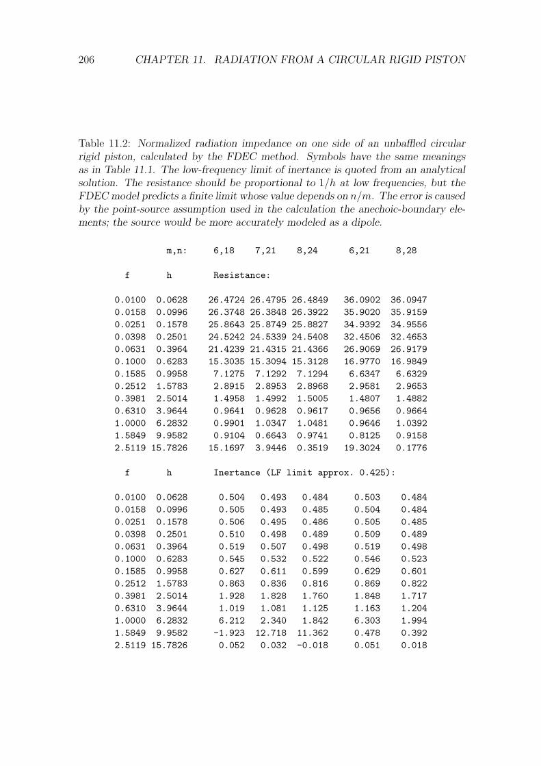
206 CHAPTER 11. RADIATION FROM A CIRCULAR RIGID PISTON
Table 11.2: Normalized radiation impedance on one side of an unbaffled circularrigid piston, calculated by the FDEC method. Symbols have the same meaningsas in Table 11.1. The low-frequency limit of inertance is quoted from an analyticalsolution. The resistance should be proportional to 1/h at low frequencies, but theFDEC model predicts a finite limit whose value depends on n/m. The error is causedby the point-source assumption used in the calculation the anechoic-boundary ele-ments; the source would be more accurately modeled as a dipole.
m,n: 6,18 7,21 8,24 6,21 8,28
f h Resistance:
0.0100 0.0628 26.4724 26.4795 26.4849 36.0902 36.09470.0158 0.0996 26.3748 26.3848 26.3922 35.9020 35.91590.0251 0.1578 25.8643 25.8749 25.8827 34.9392 34.95560.0398 0.2501 24.5242 24.5339 24.5408 32.4506 32.46530.0631 0.3964 21.4239 21.4315 21.4366 26.9069 26.91790.1000 0.6283 15.3035 15.3094 15.3128 16.9770 16.98490.1585 0.9958 7.1275 7.1292 7.1294 6.6347 6.63290.2512 1.5783 2.8915 2.8953 2.8968 2.9581 2.96530.3981 2.5014 1.4958 1.4992 1.5005 1.4807 1.48820.6310 3.9644 0.9641 0.9628 0.9617 0.9656 0.96641.0000 6.2832 0.9901 1.0347 1.0481 0.9646 1.03921.5849 9.9582 0.9104 0.6643 0.9741 0.8125 0.91582.5119 15.7826 15.1697 3.9446 0.3519 19.3024 0.1776
f h Inertance (LF limit approx. 0.425):
0.0100 0.0628 0.504 0.493 0.484 0.503 0.4840.0158 0.0996 0.505 0.493 0.485 0.504 0.4840.0251 0.1578 0.506 0.495 0.486 0.505 0.4850.0398 0.2501 0.510 0.498 0.489 0.509 0.4890.0631 0.3964 0.519 0.507 0.498 0.519 0.4980.1000 0.6283 0.545 0.532 0.522 0.546 0.5230.1585 0.9958 0.627 0.611 0.599 0.629 0.6010.2512 1.5783 0.863 0.836 0.816 0.869 0.8220.3981 2.5014 1.928 1.828 1.760 1.848 1.7170.6310 3.9644 1.019 1.081 1.125 1.163 1.2041.0000 6.2832 6.212 2.340 1.842 6.303 1.9941.5849 9.9582 -1.923 12.718 11.362 0.478 0.3922.5119 15.7826 0.052 0.032 -0.018 0.051 0.018

11.5. TRANSIENT ANALYSIS: CHECKING FOR ECHOES 207
only) and normalizing, we obtain an inertance of
m = 0.4249 (11.69)
in series with a resistance ofrs = 0.2986 h4. (11.70)
We require a parallel combination having the same asymptotic behavior at lowfrequencies. Because rs ∝ h4 in this case, the inertance is the dominant impedanceterm at low frequencies, so we require a small-rs approximation. The admittance ofthe series combination is
1jhm + rs
=1
jhm(
1 + rsjhm
) ≈1− rs
jhm
jhm=
1jhmar
+1rar
(11.71)
wheremar = m = 0.4249 (11.72)
(which is the “LF limit” given in Table 11.2) and
rar = h2m2/rs = 6.049/h2. (11.73)
So rar →∞ as h → 0. But Table 11.2 suggests that rar approaches a finite limitwhich depends on n/m. The limit is insensitive to m, indicating that FDEC ap-proximations are not the main cause of this error. (Indeed the calculated resistance,and hence the error therein, remains comparatively insensitive to m for all h < 1.)Since n/m is proportional to the distance from the origin to the simulated bound-ary, the dependence of the calculated resistance on n/m implies that the modelof the boundary is not anechoic. Having absolved the FDEC approximations, wemust attribute the non-anechoic behavior to the assumed boundary impedance. Asexplained in Subsection 6.5.4, the point-source radiation condition is not valid fora source producing a net flux of zero; Table 11.2 is the promised illustration of thiseffect.
That said, we should also note that the error in rar caused by the radiationcondition is minor compared with the error in mar caused by FDEC effects. Thecomputed low-frequency values of mar and rar give a normalized time constant ofabout 0.0134, corresponding to a transition frequency h ≈ 75, whereas the limitof the computed rar is approached for values of h less than about 0.1. The hightransition frequency indicates that the computed radiation impedance is almostpurely inductive—as it should be—as the computed rar approaches its false limit.
11.5 Transient analysis: checking for echoes
In the case of the baffled circular piston, the simulation of the anechoic boundarycondition is claimed to be a valid far-field approximation. The most direct way totest this claim is to perform a transient analysis in which we transmit a pulse fromthe source and verify that there are no significant echoes from the boundary of thesimulated region.

208 CHAPTER 11. RADIATION FROM A CIRCULAR RIGID PISTON
11.5.1 Normalized time
Because frequency in the FDEC model has been normalized, the abscissa of thetransient response will be a normalized time, denoted by t. Eq. (11.39) indicatesthat ω is normalized by multiplying by a/c. So any quantity proportional to ω−1 isnormalized by multiplying by c/a. The period T becomes
T =cTa
(11.74)
and in general,
t =cta
. (11.75)
Alternatively, we can argue that dimensionless expressions must remain invariantunder the normalization; in particular,
ωt = ht. (11.76)
Substituting from Eq. (11.39) and solving for t gives Eq. (11.75). Physically, t is theratio of the distance traveled by sound in time t to the radius of the piston.
11.5.2 The test signal
To ensure that any reflections will not be masked by time-overlap between the directand reflected signals, the pulse must be of finite duration. Furthermore, to minimizethe number of volume elements needed for the simulation, the spatial spread of thepulse and hence the duration of the pulse should be as short as possible. But thepulse cannot be made arbitrarily short; because the FDEC model is accurate onlyfor frequencies in the range |h| < m, the pulse must not contain substantial spectralenergy outside this range. Thus we require a function which is time-limited andalmost band-limited.
It is well known that a raised-cosine pulse of duration 2T has almost all of itsspectral energy in the band |ω| < 2π/T (see e.g. [40], p. 62). Indeed, it is shown inSection B.12 that only 0.0515% of the energy—corresponding to 2.27% of the r.m.s.amplitude—is outside the band |ω| < 2π/T . If this pulse has a peak amplitude of 2at time t = 0, it is described by the equation
g(t) =
1 + cos(πt
T
)
if |t| < T,
0 otherwise.(11.77)
It remains to choose a suitable T for the pulse. Recalling Eq. (11.41), let uschoose T so that no more than 0.0515% of the energy is outside the band |h| < m.As g(t) has this fraction of its energy outside the band
|ω| < 2πT
, (11.78)
our problem is to ensure that |h| < m inside this band. Eq. (11.78) can be normalized(e.g. by multiplying both sides by a/c) to obtain
|h| < 2πT
(11.79)
11.5. TRANSIENT ANALYSIS: CHECKING FOR ECHOES 209
so we can be sure that |h| < m if
2πT
< m , (11.80)
i.e. ifT >
2πm
. (11.81)
When this condition is met, less than 2.27% of the r.m.s. amplitude is outside theband |h| < m.
Condition (11.81) is just met by setting T = 6.5/m; a short T minimizes thenumber of elements required for the simulation, but severely tests the accuracybandwidth of the FDEC model.
If the test function is to be implemented in a SPICE transient analysis, it mustbe time-shifted so that it is zero for t < 0. This is accomplished by writing (t−T )for t in Eq. (11.77). We normalize the times by noting that t/T = t/T , and considerg to be a function of t. Dividing the function by 2T normalizes the magnitude sothat ∫ ∞
−∞g(t) dt = 1 (11.82)
giving a pulse of unit area2 for any value of T . Finally we put T = 6.5/m. Theresult is
g(t) =
1− cos(
mπt6.5
)
13/mif 0 < t < 13/m,
0 otherwise.(11.83)
In the model-building program the non-constant segment of g(t) is implemented bythe function “rc”. For a discussion of the code which produces the transient sourcespecification, illustrated by a listing of the specification used later in this section,see Section B.12.
It remains to decide whether the test function represents a pressure or a flux. In adiverging spherical wave, according to Eqs. (3.17) and (3.35), the pressure falls of as1/R regardless of frequency, while the velocity falls off in a more complex, frequency-dependent manner. If the waveform is a pulse whose spectrum spans a range offrequencies, the shape of the pressure wave (in time, not in space) is independent ofradius, whereas the velocity waveshape varies. But at large radii, the velocity waveapproaches geometric similarity with the pressure wave (see Subsection 3.3.5). Thuswe can fix the pressure waveshape at all radii and the velocity waveshape in the farfield by specifying the pressure at a single radius. This conclusion applies exactly toa point source; for a sufficiently small distributed source, it suggests that the sourcepressure is more similar to its far-field counterpart than the source velocity.
11.5.3 Prediction of reflections by geometrical optics
The total path lengths for reflected signals, and hence their arrival times, can becalculated by geometrical optics. If any reflections are observed in the transientresponse, the arrival times may identify the path of the reflection or at least reduce
2The area normalization was done with a view to experimenting with shorter pulses and ob-serving the finite-difference errors; but this option has not been pursued within the present thesis.

210 CHAPTER 11. RADIATION FROM A CIRCULAR RIGID PISTON
the range of possibilities. Because the geometry of the problem is determined bythe ratio n/m, we must first choose reasonable values for these variables.
For a given n/m ratio, a smaller m gives fewer elements in the model. Toensure that the model represents a distributed source and tests the claim that adistributed source has the same far-field radiation condition as a point-source, werefrain from choosing m = 1. A somewhat arbitrary compromise is m = 4. Thisgives T = 6.5/m = 1.625. Since T is the shortest period of the significant compo-nents of the test pulse (by Eq. (11.78)), the shortest significant wavelength is 1.625times the radius of the diaphragm; that is, the diameter of the source is slightlygreater than a wavelength. Thus the source is not acoustically small at all frequen-cies of interest. Moreover, because the pressure at every point on the diaphragm iscoupled to the velocities at all other points, we do not have a simple specification ofthe pressure at a single radius (i.e. over a single spherical surface). Hence we mayexpect the pressure waveform in the far field to be noticeably different from that atthe source.
Now consider the constraints on n. To avoid masking of weak reflections by thestrong direct signal, there must be no time-overlap between the direct and reflectedsignals at the test point(s). The spatial spread of the pulse is 2Tm = 13 elements,so that a clearance of at least 6.5 elements between the test point and the boundaryseems to be sufficient. The clearances should be increased, however, to allow fordistortion of the waveforms. As the direct signals have shorter paths than thereflected signals, the suppression of echoes is exaggerated by geometric spreading;to minimize this effect, the test point(s) should not be much closer to the source thanto the boundaries. These requirements have been met by taking n = 32 and usingtwo test points, denoted by A and B, at the centers of compliance elements ∆C16,7
and ∆C16,17, respectively, giving a minimum clearance of 15.5 elements between thetest points and the anechoic boundary. (The model-building program calculatesthese subscripts in terms of n to ensure that they are legal for all n.) Points A andB, together with their coordinates in terms of ∆r and ∆z, are shown in the upperinset of Fig. 11.2.
Because sound travels through a distance a in a normalized time of unity (seeEq. (11.75)), the coordinates and the overall dimensions of the model can be ex-pressed as equivalent normalized times3 by dividing by a = m∆r = m∆z, wherem = 4. Hence we can calculate the normalized propagation times of direct and re-flected signals according to geometrical (ray) optics. For the reflected rays there is noneed to calculate the coordinates of the points of reflection; as the reflecting surfacesare mutually parallel or perpendicular, it is a simple matter to locate the virtualimages of the source (which form a two-dimensional array) and find the straight-linepath lengths from the virtual sources to the observation points. (For the purpose oflocating images, the z axis can be treated as a perfect reflector because of the rota-tional symmetry. When the problem is visualized in three dimensions, the virtualimages of the origin, other than those on the z axis, are coaxial circles, not points.)The normalized propagation times are converted to normalized peak-arrival timesby adding T = 13/8, i.e. by adding the delay between t = 0 and the peak of the testpulse.
3The author resists the temptation to use the term “normalized distance” because the nor-malization process began with acoustic impedance, which depends on area, not length. If area isnormalized by dividing by πa2, distance is normalized by dividing by
√π a, which is not convenient.

11.5. TRANSIENT ANALYSIS: CHECKING FOR ECHOES 211
0
0
0
0 2 4 6 8 10 12 14 16 18 20Normalized time t = ct/a
Mean pressure over source × 120
Pressure at A
Pressure at Br z z,B
rz r, z
Residual reflections (peak)predicted by geometrical optics:
r : from boundary r = b ;z : from boundary z = b ;B : from baffle.
Unlabeled bars show direct wave.
-
6
0 a b0
b
r
z
rrA (15.5∆r, 6.5∆z)
B (15.5∆r, 16.5 ∆z)
Source
Baffle
Anechoic boundaries
Axis
a = 4 ∆r = source radiusb = 32 ∆r = 32∆z
q
q
q
q
q
q
q
q
q
q
q
q
q
q
q
q
q
q
q
q
q
q
q
q
q
q
q
q
q
q
q
q
q
q
q
q
q
q
q
q
q
q
q
q
q
q
q
q
q
q
q
q
q
q
q
q
q
q
q
q
q
q
q
q
q
q
q
q
q
q
q
q
q
q
q
q
q
q
q
q
q
q
q
q
q
q
q
q
q
q
q
q
q
q
q
q
q
q
q
q
q
q
q
q
q
q
q
q
q
q
q
q
q
q
q
q
q
q
q
q
q
q
q
q
q
q
q
q
q
q
q
q
q
q
q
q
q
q
q
q
q
q
q
q
q
q
q
q
q
q
q
q
q
q
q
q
q
q
q
q
q
q
q
q
q
q
q
q
q
q
q
q
q
q
q
q
q
q
q
q
q
q
q
q
q
q
q
q
q
q
q
q
q
q
q
q
q
q
q
q
q
q
q
q
q
q
q
q
q
q
q
q
q
q
q
q
q
q
q
q
q
q
q
q
q
q
q
q
q
q
q
q
q
q
q
q
q
q
q
q
q
q
q
q
q
q
q
q
q
q
q
q
q
q
q
q
q
q
q
q
q
q
q
q
q
q
q
q
q
q
q
q
q
q
q
q
q
q
q
q
q
q
q
q
q
q
q
q
q
q
q
q
q
q
q
q
q
q
q
q
q
q
q
q
q
q
q
q
q
q
q
q
q
q
q
q
q
q
q
q
q
q
q
q
q
q
q
q
q
q
q
q
q
q
q
q
q
q
q
q
q
q
q
q
q
q
q
q
q
q
q
q
q
q
q
q
q
q
q
q
q
q
q
q
q
q
q
q
q
q
q
q
q
q
q
q
q
q
q
q
q
q
q
q
q
q
q
q
q
q
q
q
q
q
q
q
q
q
q
q
q
q
q
q
q
q
q
q
q
q
q
q
q
q
q
q
q
q
q
q
q
q
q
q
q
q
q
q
q
q
q
q
q
q
q
q
q
q
q
q
q
q
q
q
q
q
q
q
q
q
q
q
q
q
q
q
q
q
q
q
q
q
q
q
q
q
q
q
q
q
q
q
q
q
q
q
q
q
q
q
q
q
q
q
q
q
q
q
q
q
q
q
q
q
q
q
q
q
q
q
q
q
q
q
q
q
q
q
q
q
q
q
q
q
q
q
q
q
q
q
q
q
q
q
q
q
q
q
q
q
q
q
q
q
q
q
q
q
q
q
q
q
q
q
q
q
q
q
q
q
q
q
q
q
q
q
q
q
q
q
q
q
q
q
q
q
q
q
q
q
q
q
q
q
q
q
q
q
q
q
q
q
q
q
q
q
q
q
q
q
q
q
q
q
q
q
q
q
q
q
q
q
q
q
q
q
q
q
q
q
q
q
q
q
q
q
q
q
q
q
q
q
q
q
q
q
q
q
q
q
q
q
q
q
q
q
q
q
q
q
q
q
q
q
q
q
q
q
q
q
q
q
q
q
q
q
q
q
q
q
q
q
q
q
q
q
q
q
q
q
q
q
q
q
q
q
q
q
q
q
q
q
q
q
q
q
q
q
q
q
q
q
q
q
q
q
q
q
q
q
q
q
q
q
q
q
q
q
q
q
q
q
q
q
q
q
q
q
q
q
q
q
q
q
q
q
q
q
q
q
q
q
q
q
q
q
q
q
q
q
q
q
q
q
q
q
q
q
q
q
q
q
q
q
q
q
q
q
q
q
q
q
q
q
q
q
q
q
q
q
q
q
q
q
q
q
q
q
q
q
q
q
q
q
q
q
q
q
q
q
q
q
q
q
q
q
q
q
q
q
q
q
q
q
q
q
q
q
q
q
q
q
q
q
q
q
q
q
q
q
q
q
q
q
q
q
q
q
q
q
q
q
q
q
q
q
q
q
q
q
q
q
q
q
q
q
q
q
q
q
q
q
q
q
q
q
q
q
q
q
q
q
q
q
q
q
q
q
q
q
q
q
q
q
q
q
q
q
q
q
q
q
q
q
q
q
q
q
q
q
q
q
q
q
q
q
q
q
q
q
q
q
q
q
q
q
q
q
q
q
q
q
q
q
q
q
q
q
q
q
q
q
q
q
q
q
q
q
q
q
q
q
q
q
q
q
q
q
q
q
q
q
q
q
q
q
q
q
q
q
q
q
q
q
q
q
q
q
q
q
q
q
q
q
q
q
q
q
q
q
q
q
q
q
q
q
q
q
q
q
q
q
q
q
q
q
q
q
q
q
q
q
q
q
q
q
q
q
q
q
q
q
q
q
q
q
q
q
q
q
q
q
q
q
q
q
q
q
q
q
q
q
q
q
q
q
q
q
q
q
q
q
q
q
q
q
q
q
q
q
q
q
q
q
q
q
q
q
q
q
q
q
q
q
q
q
q
q
q
q
q
q
q
q
q
q
q
q
q
q
q
q
q
q
q
q
q
q
q
q
q
q
q
q
q
q
q
q
q
q
q
q
q
q
q
q
q
q
q
q
q
q
q
q
q
q
q
q
q
q
q
q
q
q
q
q
q
q
q
q
q
q
q
q
q
q
q
q
q
q
q
q
q
q
q
q
q
q
q
q
q
q
q
q
q
q
q
q
q
q
q
q
q
q
q
q
q
q
q
q
q
q
q
q
q
q
q
q
q
q
q
q
q
q
q
q
q
q
q
q
q
q
q
q
q
q
q
q
q
q
q
q
q
q
q
q
q
q
q
q
q
q
q
q
q
q
q
q
q
q
q
q
q
q
q
q
q
q
q
q
q
q
q
q
q
q
q
q
q
q
q
q
q
q
q
q
q
q
q
q
q
q
q
q
q
q
q
q
q
q
q
q
q
q
q
q
q
q
q
q
q
q
q
q
q
q
q
q
q
q
q
q
q
q
q
q
q
q
q
q
q
q
q
q
q
q
q
q
q
q
q
q
q
q
q
q
q
q
q
q
q
q
q
q
q
q
q
q
q
q
q
q
q
q
q
q
q
q
q
q
q
q
q
q
q
q
q
q
q
q
q
q
q
q
q
q
q
q
q
q
q
q
q
q
q
q
q
q
q
q
q
q
q
q
q
q
q
q
q
q
q
q
q
q
q
q
q
q
q
q
q
q
q
q
q
Figure 11.2: FDEC calculation of the transient response at two points A and B(see upper inset) in the field of a circular rigid piston in an infinite planar baffle,in cylindrical coordinates (r, φ, z), with m = 4 and n = 32. The vertical scale isarbitrary except that the top trace (showing the initial pressure pulse produced bythe piston) is compressed by a factor of 20 relative to the other two. Vertical barsshow arrivals of direct and reflected wave crests as predicted by geometrical optics(see lower inset). Reflections from the model boundaries are weak, as intended.

212 CHAPTER 11. RADIATION FROM A CIRCULAR RIGID PISTON
The resulting arrival times are indicated by the short vertical bars in Fig. 11.2.As an aid to interpreting the time scale, note that it takes 8 units of normalizedtime for sound to travel a distance b, i.e. from the origin to the closest points on theanechoic boundary. So a time frame of 20 units includes a manageable number ofsingle and double reflections.
11.5.4 Simulation results and discussion
The top trace in Fig. 11.2 is the test pulse. The middle trace is the pressure at pointA and the bottom trace the pressure at point B. As in all graphs in this thesis, nointerpolation is used. The three pressures are plotted at the discrete times used bySPICE in the transient analysis; the variable increment used by SPICE is manifestedas a variable spacing between the plotted points. On each of the lower two traces, anunlabeled bar shows the expected arrival of the direct signal, and bars labeled “r”and “z” show the expected arrivals of the signals reflected from the constant-r andconstant-z boundaries, respectively. The bar labeled “r, z” predicts the arrival at Bof the signal reflected first by the constant-r boundary and then by the constant-z boundary; both points of reflection are near the top right hand corner of thesimulated region (as it is seen in cross-section in the upper inset). Because bothboundaries involved are meant to be anechoic, this doubly-reflected signal shouldbe much weaker than the singly-reflected signals. The same cannot be said for thesignal which strikes the constant-z boundary and the baffle before arriving at A,because a rigid baffle is totally reflective. The arrival of this signal is predicted bythe “z, B” bar on the middle trace. These are all the reflections expected within thetime frame of the graph.4
The reflections are exceedingly weak and clearly vindicate the FDEC model ofthe anechoic boundary condition. On the middle trace, we can just discern threeripples whose location and duration may be consistent with weak reflections. Thebottom trace has a more obvious double ripple at about the expected time, but theduration seems too short for a reflection of the test pulse. It is just possible thatthe two singly-reflected signals happen to cancel at B (bottom trace), where theirarrival times almost coincide, but no such possibility exists at A (middle trace). AtA, the reflected wavefront is expanding in the z direction but contracting in the φdirection; as this contraction reduces the attenuation due to geometric spreading,the weakness of the reflection from the cylindrical boundary is especially significant.
As predicted above, there is some distortion of the raised-cosine waveform be-cause the pressure is not imposed over a constant-R surface (where R is the spher-ical radial coordinate). Another possible reason for the distortion is suggested byEq. (10.63), which indicates that the FDEC method underestimates the resonancefrequencies of pipes—and hence the speed of sound—by a fraction which increaseswith frequency. This conclusion is based on Arai’s error analysis [2], which usesplane waves in Cartesian coordinates, but can be generalized in a qualitative way asfollows. If P has a spatial average of zero, so does ∇2P , so that any finite-differenceestimate of ∇2P must approach zero as the step size increases. Hence, for large step
4The first reflected signal to arrive outside the time frame strikes the constant-r boundary onthe far side of the z axis (i.e. the left side in the upper inset), and crosses the z axis on its wayto point A. Of course “point” A is really a circle about the z axis, so we may regard the samesignal as striking the constant-r boundary on the right side of the z axis, then crossing the axisand reaching point A on the left side.

11.5. TRANSIENT ANALYSIS: CHECKING FOR ECHOES 213
sizes and/or high frequencies, the FDEC method will tend to underestimate |∇2P |for given P . Now the Helmholtz equation can be written
−ω2P = c2∇2P. (11.84)
An underestimate of ∇2P unbalances this equation in the same direction as anunderestimate of c2 and therefore has a similar effect on the calculated pressuredistribution. If the FDEC model underestimates c2, and hence c, by a margin whichincreases with frequency, it effectively represents a dispersive medium in which high-frequency components of signals are delayed more than low-frequency components.This effect may be partly responsible for the overshoot and ringing in the calculatedwaveforms at A and B.
Another apparent anomaly in Fig. 11.2 is that, at both observation points, thewave peak arrives sooner than predicted by geometrical optics. There are two rea-sons for this. First, the prediction assumes that the temporal peak of the waveformcoincides with the spatial peak. But in fact, because the wave decays as it prop-agates, the envelope of the wave—i.e. the graph of the (temporal) peak pressureversus radius—is a decreasing function of radius. Hence the temporal peak occursnot at the spatial peak but rather at the point of tangency between the spatialwaveform and its envelope, and this point is on the leading slope of the wave. Sothe temporal peak arrives before the spatial peak and hence before the “predicted”time shown in Fig. 11.2. Second, because the source is distributed, and because theamplitude of the signal radiated from each point on the source decays with distance,the signals received from the near side of the source are weighted more than thosereceived from the far side. As the time delay applicable to the near side of the sourceis shorter, the weighting of the near side reduces the delay of the peak of the totalsignal. Both of these effects become less pronounced as the propagation distanceincreases; hence the arrival times of the reflected signals should be more accuratelypredicted than those of the direct signals.
In summary, the FDEC model of the free-air boundary has been tested in thetime domain, at several angles of incidence, using a pulsed signal containing the fullrange of frequencies over which the FDEC method is claimed to be reliable under themost favorable conditions (plane waves and Cartesian coordinates). Although theseconditions did not hold, the simulated boundary was found to be nearly anechoic,as intended.

Chapter 12
Conclusions
From the large volume of theory and computation in this thesis, together with thenumerous references to possible extensions or improvements of the models, it canbe seen that the linear modeling of loudspeaker components was and remains afertile area of research. The restriction to linear models does not greatly diminishthe usefulness of this work, because the linear distortions of loudspeakers are acontinuing problem in analysis and design. Moreover, linearity makes the problemtractable, so that there is no excuse for not attempting a solution. This thesisdoes not come close to offering a complete solution—for example, it does not (yet)allow for non-local boundary conditions caused by non-rigid walls—but it offersan equivalent-circuit model of a loudspeaker which, unlike older equivalent-circuitmodels, takes account of the wave-like nature of the acoustic field in the enclosureand the effects of the resulting resonances on the system response. The ability topredict the response of a given system is of course a first step towards designing asystem with a prescribed response.
In the presentation of the foundations of linear acoustics, much theoretical econ-omy has been achieved by using the techniques of vector analysis to derive thefundamental equations in a hierarchy of forms. The “one-parameter” or “1P” formshave been expressed with novel generality. These apply to a “1P” pressure field,which is initially defined as a field in which the excess pressure depends on only onespatial coordinate ξ measuring arc length normal to the constant-ξ surfaces (isobaricsurfaces).
The equation of motion, which expresses Newton’s second law for a non-viscousfluid, has a sequence of forms in which each form inherits the assumptions of itspredecessor. The most general integral form applies to a closed surface moving withthe fluid. The linearized point form (differential form) assumes irrotational flow, lowgravity, and small oscillations and compressions. In a 1P pressure field, this pointform can be integrated to obtain the 1P form, which applies to normal oscillations ofa uniform thin shell between two isobaric surfaces. The 1P form leads to the conceptof distributed acoustic mass, whose electrical analog is distributed inductance. Ifthe fluid is assumed incompressible in some region, the 1P form can be integratedto give a fourth form, which applies to ports or vents and leads to the concept of(lumped) acoustic mass, whose electrical analog is (lumped) inductance.
The equation of continuity expresses conservation of mass and, when combinedwith a relationship between pressure and density, yields the equation of compression.The integral form of the equation of continuity applies to a stationary closed surface.
214

215
If we assume small compressions and barotropic conditions, we obtain the linearizedpoint form (differential form) of the equation of compression, which can be integratedover a fixed volume to obtain the integral form of the equation of compression. Thisform leads to two others. The first assumes uniform excess pressure throughout thevolume, and leads to the concept of (lumped) acoustic compliance, whose electricalanalog is (lumped) capacitance. The second is the 1P form, which applies to auniform thin shell between two isobaric surfaces in a 1P pressure field. The 1P formleads to the concept of distributed acoustic compliance, whose electrical analog isdistributed capacitance. Thus the four forms of the equation of compression do notform a linear sequence.
The point forms of the equations of motion and compression lead to the waveequation, while the 1P forms lead to Webster’s horn equation. Both equations applynot only to the excess pressure, but also to the velocity potential, whose existence isguaranteed by the linearizing assumptions. Provided that the compressibility of airis explicitly represented by compliance elements, Kirchhoff’s laws are applicable tothe pressures and fluxes in lumped acoustic masses and compliances, so that thesecomponents can legitimately be connected into “acoustic circuits”.
The well-known “Webster” horn equation has been placed on a new theoreticalfoundation which assumes (exact or approximate) 1P waves. This approach removesany a priori assumption concerning the wavefront shape, but leads to the conclusionthat there are only three wavefront shapes allowing exact 1P propagation.
Webster’s equation follows exactly from the 1P forms of the equations of motionand compression. The ξ coordinate is the axial coordinate of the horn while S(ξ) isthe area of a constant-ξ surface segment bounded by a tube of orthogonal trajectoriesto all the constant-ξ surfaces; such tubes (and no others) are possible boundarysurfaces for a horn satisfying Webster’s equation in ξ. As far as the derivationof Webster’s equation is concerned, the shape of the wavefront (isobaric surface)is arbitrary—in particular, it is not necessarily planar. Note that S(ξ) must becalculated from the actual wavefront, and not from a tangent plane.
It has also been shown that the Helmholtz equation admits solutions dependingon a single spatial coordinate u if and only if |∇u| and ∇2u are functions of u alone.The |∇u| condition allows u to be transformed to the coordinate ξ which measuresarc length normal to the isobaric surfaces; that is, |∇ξ| = 1. Hence, in the initialdefinition of a “1P” pressure field, the normal-arc-length condition is redundant, andthe definition can be weakened accordingly. The condition that |∇ξ| = 1 yields anexpression for the Laplacian of a 1P pressure field, from which it has been shown thewave equation reduces exactly to Webster’s horn equation; this is a second derivationmaking no a priori assumption concerning the wavefront shape.
A 1P acoustic field has uniform excess pressure, uniform velocity potential, nor-mal and uniform fluid velocity and uniform intensity over every isoparametric sur-face (wavefront), and exhibits rectilinear propagation; these conditions apply at allfrequencies. The conditions on excess pressure, velocity potential and velocity areequivalent, so there is no ambiguity in the description “1P”.
The only coordinates admitting exact 1P waves are those whose level surfaces areparallel planes or coaxial cylinders or concentric spheres; consequently, the guidingsurface of an exact 1P waveguide must be a cylinder or a cylindrical sector or a cone,respectively. The proof of this fact is complex and depends on most of the theoryleading to the general derivation of Webster’s equation in a coordinate admitting 1P

216 CHAPTER 12. CONCLUSIONS
waves. Hence, although it is possible to obtain Webster’s equation from the waveequation in each of the three permitted coordinates, the general derivation requiresless supporting theory. The general derivation also reveals the common feature ofall 1P acoustic fields which makes Webster’s equation applicable: such fields can bedescribed in terms of a normal-arc-length coordinate.
A true 1P waveguide must be infinite, but if a 1P waveguide is truncated, itwill remain approximately 1P at sufficiently high frequencies, and will thereforeapproach constant directivity as the frequency is increased; the constant directivityis confined to the near field for a cylindrical tube and for a cylindrical sectorial horn,but extends to the far field for a conical horn.
Webster’s equation is approximately true for a horn carrying an approximately1P wave. A tube or horn is approximately 1P if
(a) the cross-section remains small compared with the wavelength and varies grad-ually (i.e. changes by a small fraction in a distance comparable with the cross-sectional dimensions) and any curvature in the centroidal axis has a radiusmuch larger than the cross-sectional dimensions, or
(b) the cross-section is large, but the tube or horn has a shape approximating thatof one of the three families of exact 1P waveguides and is uniformly drivenover one isoparametric cross-section, and the dimensions of the mouth (for atruncated horn) are much larger than a wavelength, or
(c) condition (a) holds for part of the length (possibly including the driving point)and condition (b) holds for the remainder.
A practical 1P horn having nearly constant directivity in the far field must bebased on a conical horn. Directivity may be controlled by shaping the cross-sectionof the cone, and the loading characteristics (predicted by Webster’s equation) may bevaried by departing from the conical shape in the region of small cross-section. Butsuch adjustments are only evolutionary; the design of practical constant-directivityhorns cannot be fundamentally advanced by finding a new geometry for an exact1P waveguide, because all possible 1P wavefront shapes are already known.
The finite-difference equivalent-circuit (FDEC) method for modeling acousticfields has been extended to include 1P horns, three-dimensional fields in curvilinearorthogonal coordinates, 3D boundary conditions, and fiber-damped regions. Thepractical feasibility of the method has been illustrated with two computational ex-amples, the first of which predicts the effects of internal resonances on the frequencyresponse of a loudspeaker.
A finite-difference approximation to Webster’s equation yields the nodal equa-tions of an L-C ladder network, while a similar approximation to the wave equationin general curvilinear orthogonal coordinates yields the nodal equations of a three-dimensional L-C network. The same circuits can be obtained from the equationsof motion and compression, confirming that “current” in the equivalent circuit isvolume flux.
The topology and component values of the undamped 3D model are quite in-tuitive. The region to be simulated is divided into contiguous quasi-rectangularvolumes, which are the compliance elements. The mass elements are also contigu-ous and quasi-rectangular, but are displaced (relative to the compliance elements)

217
by a half-element in each of the three coordinate directions. The value of each com-ponent is found by assuming that it is a rectangular prism, calculating its dimensionsfrom the scale factors at its center (i.e. for the central values of the coordinates),and using the usual lumped-component formulae. For the truncated elements at theboundaries of the model, the same rules are applied to the reduced ranges of thecoordinates. In all cases, pressure is sampled at the centers of two opposite facesof each mass element and at the body-center of each compliance element. For thepurpose of calculating the fluxes through the six faces of each compliance element,velocities and scale factors are sampled at the centers of the faces. The scale factorsat the centers of boundary surface elements are used to convert velocities to fluxeswhen applying boundary conditions.
The effects of fibrous filling materials can be represented by modifications to theequivalent circuit. The free-air components are retained in the model, except thattheir values are slightly changed because the fiber reduces the effective volumes andcross-sectional areas. A parallel mass-resistance combination appears in series witheach mass element. The flux through the added mass represents motion of the fibers,while the flux through the added resistance represents motion of the air relative tothe fibers. A series compliance-resistance combination appears in parallel with eachcompliance element. The time constant of the added R-C combination is the thermaltime constant of the air-fiber system at constant pressure, while the time constantof the resulting C-R-C loop is the thermal time constant at constant volume. Twomore time constants can be defined by fixing the fiber temperature, and one moreby fixing the air temperature. All five time constants can be expressed in term ofone of them, denoted by τfp, which is defined for constant fiber temperature andconstant pressure. This can be calculated for practical purposes from the formula
τfp ≈d2
8α(m2 −m0.37) ln
(
m+12
)
where d is the fiber diameter, α is the thermal diffusivity of air, f (not in the formula)is the fraction of the overall volume occupied by the fiber, and m = f−1/2.
The thermal diffusivity (used in the above formula) is just one of the propertiesof air that affect the values of the FDEC elements. With the exception of the ab-sorption coefficient (which does not appear in the models), all the linear acousticalproperties of air can be calculated with acceptable accuracy from the temperatureand pressure, using simple algebraic formulae which assume dry air. These formu-lae are sufficient for the analysis of small acoustic devices, in which atmosphericabsorption is not a major contributor to damping.1
When constructing an FDEC model of a moving-coil loudspeaker in an enclo-sure, one must allow for the sharing of the diaphragm area between several volumeelements. This can be accomplished by redrawing the conventional equivalent circuitof the driver so that it includes a transconductance instead of a transfer resistance,and partitioning the transconductance in the same fractions as the diaphragm area.The ratios of the jth partial flux to the common back e.m.f. and of the jth partialcurrent to the jth developed pressure are equal to the jth partial transconductance.
In the FDEC model of a particular driver in a particular fiber-filled box, the1Formulae for the absorption coefficient, which is sensitive to humidity as well as temperature
and pressure, may be found in ANSI S1.26-1978 [41].

218 CHAPTER 12. CONCLUSIONS
following observations have been made by neglecting selected components and com-paring the response with that of the full simulation:
• Viscosity is the dominant mechanism of damping, thermal relaxation being ofsecondary importance;
• The neglect of internal elastic forces in the fibers is justified;
• The departure from thermal equilibrium (which occurs at high frequencies)has very little effect on the frequency response;
• While the addition of fiber increases the output at infrasonic frequencies, itreduces the output in the bass rolloff region and does not lower the 3 dB rollofffrequency; this conclusion applies not only to the overall effect of the fiber,but also to its thermal capacity alone.
All four observations are expected to be almost universally true—the first becauseit is so pronounced, and the others because they are consistent with qualitativepredictions.
The classical problem of the circular rigid-piston radiator has been used to testthe FDEC method in cylindrical coordinates with a free-air (anechoic) boundarycondition. In the baffled version of the problem, the calculated radiation impedancedepends more on the step size than on the distance to the anechoic boundary,indicating that the boundary impedance is accurately modeled. In the unbaffledversion, at extremely low frequencies, the calculated parallel resistance dependsmore on the distance to the boundary, supporting the theoretical prediction that theanechoic boundary condition, which is calculated for a point-source, is not accuratefor a dipole source. In the baffled case, the FDEC model of the free-air boundaryhas been tested in the time domain, at several angles of incidence, using a pulsedsignal containing a comprehensive range of frequencies. The small amplitudes ofthe calculated echoes provide direct confirmation that the “anechoic” boundary isaccurately represented.
12.1 Further work
The undamped FDEC method could be used to determine the loading and direc-tional characteristics of a wide variety of infinite and truncated acoustic waveguides,some of which have been proposed by Geddes [18]. Each analysis requires an or-thogonal coordinate system with known scale factors, and is greatly facilitated if theguiding surface is an equicoordinate surface, but the coordinate system need not beseparable.
While the conditions under which a coordinate system admits one-parameterwaves have been rigorously studied in this thesis, the discussion of the existenceof two-parameter waves has been confined to the issue of what we mean when wesay “By symmetry, the pressure is independent of. . . ”. A similarly rigorous studyof two-parameter waves would be of interest because of the computational savingsthat follow from a reduction to two dimensions.
The loudspeaker model presented in this thesis does not allow for cabinet-wallvibrations. It may be possible to include these effects in the FDEC model using

12.1. FURTHER WORK 219
finite-difference approximations to the equations describing flexural vibrations ofplanar sheets. The non-local nature of the boundary impedance presented by thewall would probably be expressed by coupled flux sources. Expected difficultiesinclude edge conditions (coupling of panel motions through the corners of the box)and radiation loading. It may also be possible to model flexure of the diaphragmusing the same technique.
The equation used for estimating the pneumatic resistivity of loosely-packedfibrous filling material (Eq. (7.33)) is believed to be much less accurate than that usedfor calculating the basic air-fiber thermal time constant (Eq. (7.119), quoted above).Unfortunately the pneumatic resistivity has been found to be the more importantof the two quantities for the damping of resonances in loudspeaker enclosures, sothat further work on the estimation of pneumatic resistivity is warranted. This workwould involve the Navier-Stokes equations rather than the heat equation, and wouldrequire an averaging over possible orientations of the fibers; hence it would be moredifficult than the estimation of the thermal time constant.
Other desirable improvements to the FDEC model-building program for the loud-speaker have been mentioned in the text and appendices, and are briefly reviewedhere:
• The model could be extended to three dimensions and modified to take accountof the precise diaphragm shape and the presence of the spider and magnetassembly.
• Restrictions on the topology and dimension-ratios of the box should be loos-ened.
• Elevation of the internal temperature of the box should be modeled.
• Alternative means of specifying the driver parameters should be allowed.
• The range of available graphs should be widened.
• The handling of input should be made more robust, e.g. to remove possiblesources of floating-point exceptions.
• Specifications of boxes and drivers should be stored in files.
• The model builder and the circuit simulator should have a common interactiveshell. More functions and options should be made interactive.
• The interface to SPICE should be at a lower level than that provided by thestandard command cards.
The model-building program used in this thesis was developed to a level sufficientfor its primary purpose: to include an approximate model of the spatial variation ofpressure throughout the interior of the box and across the back of the diaphragm,and hence predict the effects of internal aeroacoustic resonances on the response ofthe loudspeaker.
The FDEC model of the loudspeaker-box system was developed with a view toanalyzing box designs intended to suppress or control the effects of internal reso-nances. In this thesis it was possible to include only a simple fiber-filled design. The

220 CHAPTER 12. CONCLUSIONS
author initially intended to include a study of alternative box topologies incorpo-rating internal acoustic filters (combinations of chambers and vents, analogous tocapacitors and inductors) designed to ensure that all parts of the enclosure behaveapproximately as lumped components. The adequacy of that approximation was tobe assessed by the FDEC method. However, because of the unexpected expansionof other parts of the thesis, including the work on 1P acoustic fields and the air-fiberthermal time constant, the study of anti-resonant box designs must be reserved fora future project.

12.1. FURTHER WORK 221

Appendix A
Somigliana’s letter to Atti Torino(1919)
The following is a paraphrase of the letter “Sulle relazioni fra il principiodi Huygens e l’ottica geometrica” by Carlo Somigliana, which appeared inAtti della Reale Accademia delle Scienze di Torino, vol. 54, no. 14a (1919),pp. 974–9. The Italian text was translated orally by Br. A. Moss, who wasthen at the Department of Studies in Religion, University of Queensland. Inthis English version, the author has removed much redundancy and circum-locution, introduced the Gibbs vector notation (which radically changes theappearance of most equations), replaced Somigliana’s symbols with the sym-bols used elsewhere in this thesis, and added some explanatory clauses. Theuse of italics follows that in the original letter.
The two footnotes referring to the works of Laura and Bianchi are foundin Somigliana’s letter and are here labeled “(Original)”. Other footnotes areexplanatory notes added by the present author.
The letter shows that there are only three possible geometries in which asolution to the wave equation depends on only one spatial coordinate and hasparallel level surfaces, namely those in which the level surfaces are parallelplanes, coaxial cylinders, and concentric spheres.
222

223
On the Relations between Huygens’Principle and Geometrical Optics
Note of the resident National Associate CARLO SOMIGLIANA
The triply orthogonal system comprising a series of parallel surfaces and the rowsof common perpendiculars along their lines of curvature1 constitutes a complete andsimple model of the propagation of waves in an isotropic medium according to Huy-gens’ principle. The successive parallel surfaces, each of which may be regarded asthe envelope of a set of spheres with equal radii and centered on a preceding surface,are the wavefronts. The common perpendiculars may be considered as the rays cor-responding to these waves. According to Malus’s theorem2, the laws of rectilinearpropagation and of reflection and refraction find a complete representation.
However, if this model, which constitutes the foundation of geometrical optics,is to be reconciled with the theory of mechanical and electromagnetic propagation,one must find solutions of the wave equation
∂2φ∂t2
= c2∇2φ (A.1)
(where φ is the wave function, t the time, and c the velocity of propagation) for whichthe constant-φ surfaces at any instant are parallel. Three special cases of this are wellknown: spherical, planar and cylindrical waves. But it can be shown that these arethe only cases, so that there is a substantial difference between geometrical optics andthe optics of mechanical and electromagnetic vibrations. Therefore a justification ofHuygens’ principle and of rectilinear propagation can be found only in the theory ofretarded potentials, and in the hypotheses on extremely short wavelengths developedby Kirchhoff in his classic dissertation Zur Theorie der Lichtstrahlen of 1882.
A contrary result to that stated above was recently obtained by Prof. E. Laurain an article3 included in the volume Scritti matematici offerti ad Enrico D’Ovidio,published last year upon his [D’Ovidio’s?] retirement from teaching. In this verybrief note, I show how one can arrive at the correct result directly and simply,avoiding the extrapolations to the limit which Laura uses but does not exhaustivelydiscuss.
1This description assumes that the orthogonal trajectories to a family of parallel surfaces arestraight lines (see Theorem 5.1) and that a perpendicular moving along the lines of curvature ofone surface will trace out orthogonal curves on the other parallel surfaces (see Theorem 5.2 andthe surrounding paragraphs in Section 5.4).
2This theorem, also known as the Malus-Dupin theorem, concerns the equivalence of the ray-based and wave-based formulations of the laws of reflection and refraction. The assemblage ofnormal lines to a surface Σ0 is called a normal congruence. Eq. (5.26) in the proof of Theorem 5.2implies that a normal congruence is cut orthogonally by infinitely many parallel surfaces; sincet0 is normal to n, so is t. Now the Malus-Dupin theorem states that a normal congruence ofrays remains a normal congruence when subjected to any number of reflections and refractions atsmooth surfaces separating homogeneous media. If the normal surfaces to the rays are understoodas wavefronts, the truth of the theorem becomes obvious; but the theorem can also be proven byray-based methods [61, vol. 1, pp. 196–8].
3 (Original) E. Laura, Sopra la propagazione di onda in un mezzo indefinito.

224 APPENDIX A. SOMIGLIANA’S LETTER TO ATTI TORINO (1919)
Let r0 be the position vector of a point of the initial surface (denoted by Σ0) ina series of parallel surfaces, and let u, v be the parameters of this surface, so that
r0 = r0(u, v). (A.2)
We assume that in some 3D region containing a segment of this surface, every pointin space may be uniquely specified by its perpendicular distance from Σ0 (positiveon one side of the surface and negative on the other) together with the parametersu and v of the point r0 at the foot of the perpendicular; that is, we assume that wecan use (u, v, r) as coordinates. Letting r be the position vector of a general pointin the 3D region, we will have
r(u, v, r) = r0(u, v) + r n(u, v) (A.3)
where n is the unit normal to Σ0 in the sense of increasing r.4
If ds denotes the linear element of the space, we have
ds 2 = dr.dr. (A.4)
Taking differentials of Eq. (A.3) and substituting into Eq. (A.4), and using the rela-tions
ds02 = dr0.dr0
n.n = 1 ; n.dn = 0
n.dr0 = 0 ,
we obtainds 2 = ds0
2 + r2 dn.dn + dr 2 + 2r dr0.dn. (A.5)
In Eq. (A.5), ds0 represents the linear element of the surface Σ0. If we now adoptthe lines of curvature (which are orthogonal) as the parametric curves on Σ0, thislinear element will satisfy
ds02 = h2
u0 du 2 + h2v0 dv 2 (A.6)
where hu0 and hv0 are the scale factors of u and v respectively on Σ0. The last dotproduct in Eq. (A.5), with a change of sign, is the second fundamental quadraticdifferential form of the surface Σ0. So we may write5
dr0.dn =h2
u0
R0du 2 +
h2v0
S0dv 2 (A.7)
where R0 and S0 are the normal radii of curvature of the surface Σ0 in the u and v4Somigliana uses Cartesian coordinates instead of “r” and “r0”, and direction cosines instead
of “n”.5 (Original) V. Bianchi, Lezioni di Geometria differenziale (Pisa, 1902), vol. 1, p. 131.

225
directions, respectively.6 With these notations, we know that7
dn =1R0
∂r0
∂udu +
1S0
∂r0
∂vdv. (A.8)
If we dot-multiply each side of this equation with itself and use the orthogonalityof the coordinates, we obtain
dn.dn =h2
u0
R20
du 2 +h2
v0
S20
dv 2. (A.9)
Substituting Eqs. (A.6), (A.7) and (A.9) into Eq. (A.5) yields the useful form
ds 2 =(
1 +r
R0
)2h2
u0 du 2 +(
1 +rS0
)2h2
v0 dv 2 + dr 2. (A.10)
From Eq. (A.10), the scale factors hu,hv,hr for the triply orthogonal coordinatesu, v, r are8
hu = hu0
(
1 +rR0
)
; hv = hv0
(
1 +rS0
)
; hr = 1. (A.11)
Knowing the scale factors, we can write the wave equation (A.1) in the coordinates(u, v, r) and simplify it for the case in which φ is a function of r and t only.9 The
6Although Somigliana evidently did not obtain Eq. (A.7) from Eq. (A.8), it is permissible to doso because the derivation of Eq. (A.8) need not depend on Eq. (A.7) (see next footnote). By thechain rule,
dr0 =∂r0
∂udu +
∂r0
∂vdv.
If we dot-multiply this equation with Eq. (A.8), noting that
∂r0
∂u.∂r0
∂u= h2
u0 ;∂r0
∂v.∂r0
∂v= h2
v0 ;∂r0
∂u.∂r0
∂v= 0
because of the orthogonality of the coordinates, we obtain Eq. (A.7).7On Σ0, we have by Rodrigues’ theorem [60, pp. 59–60]
∂n∂u
= −Ku0∂r0
∂u=
1R0
∂r0
∂u
where Ku0 is the principal curvature in the u direction; the signs indicate that Ku0 is positive fora surface which is concave in the direction of n, while R0 is positive for a surface which is convexin that direction. Similarly,
∂n∂v
= −Kv0∂r0
∂v=
1S0
∂r0
∂v.
These two equations may be used with the chain rule
dn =∂n∂u
du +∂n∂v
dv
to obtain Eq. (A.8).Somigliana describes R0 and S0 loosely as the radii of curvature of the parametric curves; but the
derivation of Eq. (A.8) using Rodrigues’ theorem, which involves the principal (normal) curvatures,suggests that the curvatures are meant to be resolved in the n direction.
8Somigliana gives these results in terms of E and G, where E = h2u and G = h2
v.9This is the first use of the one-parameter assumption; the assumptions of parallel wavefronts
and rectilinear propagation were introduced in the opening paragraph. Before assuming 1P waves,Somigliana gives expressions for ∆1φ (= |∇φ|2) and ∆2φ (= ∇2φ), where φ is allowed to dependon u, v, r and t; as no further use is made of these expressions, they are not reproduced here.

226 APPENDIX A. SOMIGLIANA’S LETTER TO ATTI TORINO (1919)
result is∂2φ∂t2
= c2
∂2φ∂r2 +
( 1R0 + r
+1
S0 + r
) ∂φ∂r
. (A.12)
If this equation is to have a solution depending on r and t only, we must have10
1R0 + r
+1
S0 + r= 2H(r) (A.13)
where H(r) is some function of r alone. Now, a simple geometric considerationindicates that the radii of curvature of the surface at distance r from Σ0 must be11
R = R0 + r ; S = S0 + r. (A.14)
Using these relations, Eq. (A.13) may be written
H(r) =12
( 1R
+1S
)
(A.15)
showing that H(r) is the mean curvature of the surface at distance r from Σ0. Sincethis is a function of r only, the mean curvature of every parallel surface must beconstant over the surface. As Σ0 is one such surface, its mean curvature is alsoconstant.
Using a common denominator, Eq. (A.13) can be rewritten
rK0 + H0
r2K0 + 2rH0 + 1= H(r) (A.16)
whereH0 =
12
( 1R0
+1S0
)
(A.17)
K0 =1
R0S0. (A.18)
Comparing Eqs. (A.13) and (A.17), we see that H0 = H(0); i.e. H0 is the meancurvature of Σ0, which is constant. Eq. (A.18) indicates that K0 is the Gaussiancurvature of Σ0. Solving Eq. (A.16) for K0, we obtain
K0 =(2rH0 + 1) H(r)−H0
r − r2H(r). (A.19)
Since H0 is constant, K0 is a function of r only; but K0, being a property of onesurface Σ0, is also independent of r, and must therefore be constant like H0. Hence,by inverting Eqs. (A.17) and (A.18), we can show that the principal curvaturesR0 and S0 are constant over the initial surface Σ0; that is, the surface Σ0 mustbe planar (R0 = S0 = ∞), circular-cylindrical (R0 = constant, S0 = ∞) or spherical(R0 = S0 = constant).12 This conclusion applies to all the parallel surfaces becauseof the generality of Σ0.
10Here Somigliana reasons that if the solutions of the differential equation are independent ofu and v, so are the coefficients. Compare this with Eqs. (4.23) and (4.24), which imply that thecoefficients of Eq. (4.15) are functions of u alone.
11For a proof, see Subsection 5.4.1. Somigliana states these relations immediately afterEq. (A.11).
12For a justification of this logical leap, see Lemma 5.2 and Theorem 5.4 (in Chapter 5).

227
When the appropriate values of R0 and S0 are substituted into Eq. (A.12), withthe origin of r chosen to make each “constant” equal to zero, we obtain the familiarforms of the wave equation in the three coordinate systems. For the planar andspherical cases, the admissible solutions are respectively
φ = f(r − ct) + g(r + ct) (A.20)
andφ =
1r
f(r − ct) +1r
g(r + ct), (A.21)
and the cylindrical case admits solutions given by Poisson integrals:13
φ =∫ π
−πf(r sin α− ct) dα +
∫ π
−πg(r sin α + ct) dα. (A.22)
If, instead of the wave equation, we consider Laplace’s Equation, i.e. if we supposethat φ is independent of time, the above results lead to the following conclusion:
The only Newtonian distributions of mass for which the gravitational equipoten-tial surfaces outside the distribution are parallel are those whose equipotentials areplanar, circular-cylindrical or spherical.
13Somigliana omits the first integral, but the admissibility of the second integral implies that ofthe first because the wave equation is even in c. Each term in the solution can be verified by directsubstitution into the wave equation. The functions f and g are arbitrary except that they mustbe smooth enough to permit two differentiations under the integral sign; it is sufficient that theyare everywhere twice continuously differentiable (cf. [53], p. 163).

Appendix B
Program listings and explanatorynotes
B.1 IVP solver and modified Newton method
The #include file stepstat.c implements the functions Step(µ) and s(n, µ), whichare defined in Table 8.1 and used throughout Chapter 8. The file contains copiouscomments, which will be supplemented rather than repeated in the text.
The long introductory comment explains how the third-order iterative solutionscheme of step(mu) is derived from the second-order IVP. In the notation of Sub-section 8.2.4, the body of the function step(mu) would be written
yi+1 = yi + hy′i + 12h
2 y′′i + 16h
3 y′′′i (B.1)y′i+1 = y′i + hy′′i + 1
2h2 y′′′i (B.2)
i := i + 1 (B.3)xi = 1 + ih (B.4)
y′′i = −(
µ2yi +y′ixi
)
(B.5)
y′′′i =( 1
xi2 − µ2
)
y′i −y′′ixi
. (B.6)
The order of evaluation is chosen so that, after each iteration, x, y and all threederivatives of y are simultaneously available for the same i. The new values of y andy′ are estimated using truncated Taylor expansions, whereas the new values of y′′
and y′′′ are found directly from the differential equation using the newly-incrementedi. To maximize the versatility of the function, the old values are not overwrittenbut are accumulated in externally-declared arrays.
For each step, the dominant error in y′i+1 is proportional to h3. The number ofsteps taken to reach the nth stationary point is proportional to h−1. Hence the errorin s(n, µ) due to the IVP solver is approximately proportional to h2. (The truncatedTaylor expansion for yi+1 has one more term than that for y′i+1, so that the error iny for a particular x is approximately proportional to h3 rather than h2. Thereforethe iterative scheme is described as “third-order”, although it is only second-orderfor purposes involving y′.)
If y′i−1 and y′i are not strictly of the same sign, step(mu) has reached or justpassed a zero of y′. The function s(n,mu) steps up to or just past the nth zero of
228

B.1. IVP SOLVER AND MODIFIED NEWTON METHOD 229
y′, then finds the zero using one step of the “modified” or “third-order” Newtonmethod. This method was derived independently by the author and will thereforebe described here, although it is likely that the same method is described somewherein the vast mathematical literature.
The purpose of the third-order Newton method is to find a root x of the equationy(x) = 0. If xk is an estimate of the root, a single step of the method gives animproved estimate xk+1. Let
x = x(y) = x(y(x)) (B.7)
so that the desired root is x(0). If x(y) is sufficiently differentiable, we may use theTaylor expansion
x(y + ε) = x(y) + εx′(y) + 12ε
2 x′′(y) + O(ε3) (B.8)
where the “error term” O(ε3) is approximately proportional to ε3 for small ε. Dif-ferentiating Eq. (B.7) w.r.t. x and solving for x′(y) gives
x′(y) =1
y′(x). (B.9)
Differentiating again w.r.t. x and solving for x′′(y) gives
x′′(y) = − y′′(x)[y′(x)]3
. (B.10)
Because we want Eq. (B.8) to give us x(0), we put y + ε = 0, whence
ε = −y. (B.11)
Substituting Eqs. (B.9) to (B.11) into Eq. (B.8), and putting x = xk and y(xk) = yk,we obtain
x(0) = xk −yk
y′k− yk
2 y′′k2(y′k)3 − O(yk
3). (B.12)
The well-known Newton-Raphson method uses just the first two terms on theright of Eq. (B.12). The dominant error term is proportional to yk
2, which in turn isapproximately proportional to [xk − x(0)]2 if the problem is well-conditioned. Thusthe classical Newton-Raphson method is second-order: the error in xk+1 is roughlyproportional to the square of error in xk.
As the reader will have anticipated, the “modified” Newton method uses thefirst three terms on the right of Eq. (B.12). The remaining error is approximatelyproportional to yk
3, so the method is third-order.Both the classical method and the modified method come from the same Taylor
expansion of x(y). Whereas the classical method is exact for linear functions, themodified method is exact if x is a quadratic function of y (so that Eq. (B.8) is exactwithout the error term). Thus the modified method is an obvious extension of theclassical method.
The function s(n, µ) finds a zero of y′ rather than y, so that every “y” inEq. (B.12) must be given an extra prime (′). Only a single iteration is used. Theinitial estimate is xi, where i denotes the ith iteration of the IVP solver Step(µ), not

230 APPENDIX B. PROGRAM LISTINGS AND EXPLANATORY NOTES
the ith iteration of the modified Newton method. Thus, using the form of Eq. (B.12),the last statement in the function s(n,mu) would be written
s(n, µ) = xi −y′iy′′i
− (y′i)2 y′′′i
2(y′′i )3 . (B.13)
This formula is convenient to use because all the necessary values of y and itsderivatives are available from the IVP solver.
The error in s(n, µ) caused by the modified Newton method is approximatelyproportional to the cube of the difference between xi and s(n, µ), which difference isless than the step size h. Hence the error due to the modified Newton method is atworst third-order w.r.t. h, whereas the error due to the IVP solver, as noted above,is second-order. Therefore, if h is sufficiently small, the overall algorithm for findings(n, µ) is second-order, and the modified Newton method does not significantlycontribute to the error.
Of course, step(mu) can easily be modified to solve a different IVP, whiles(n,mu) can be modified to handle a boundary condition involving y instead ofy′. Thus the two functions can serve as templates for solving other Sturm-Liouvilleproblems which may arise in future work. For this reason, the author has chosento ignore the fact that the problem of Chapter 8 can be solved in terms of Besselfunctions.
A listing of the file stepstat.c follows.
/** #include file ‘stepstat.c’ (Gavin R. Putland)** DIFFERENTIAL EQUATION SOLVER, STATIONARY POINT FINDER* AND ASSOCIATED GLOBAL VARIABLES (EXCEPT h AND max).** STEP SIZE h AND MAXIMUM NO. OF STEPS max* ARE EXTERNALLY DECLARED OR #defined IN CALLING PROGRAM.** FUNCTION s(n,mu) RETURNS THE ABSCISSA OF THE nth STATIONARY POINT* OF y(x), WHERE y(x) IS THE SOLUTION TO THE INITIAL VALUE PROBLEM** y’’ + (1/x) y’ + mu^2 y = 0 (1)* y(1) = 0 (2)* y’(1) = 1. (3)** FUNCTION s(n,mu) REPEATEDLY CALLS FUNCTION step(mu),* WHICH PERFORMS ONE STEP OF THE IVP SOLUTION FOR GIVEN mu.** To obtain a third-order method of solving the IVP, we note that* Eqs. (1), (2) and (3) give** y’’(1) = -1. (4)** Then we differentiate (1) wrt x to obtain** y’’’ + (1/x) y’’ + (mu^2 - 1/x^2) y’ = 0. (5)** Eqs. (5), (2), (3), (4) constitute a new IVP. Eq. (5) is solved for* y’’’, and successive values of y’’, y’ and y can be found using first-,

B.1. IVP SOLVER AND MODIFIED NEWTON METHOD 231
* second- and third-order truncated Taylor series. But it is better to* obtain y’’ from (1) and use Taylor series for y’ and y only. For* initializing the loop, Eqs. (5), (2), (3), (4) yield** y’’’(1) = 2 - mu^2.** Because we are seeking a zero of y’, convergence of the method is* second-order; i.e. the error in s(n,mu) is roughly proportional to h^2.*/
/* GLOBAL VARIABLES FOR ITERATIVE SOLUTION OF IVP: */float x[max], ydd[max], yddd[max]; /* single precision increments */double y[max], yd[max]; /* double precision accumulation */int i; /* step counter */
/* See above comment on h and max. */
void step(float mu)
/** i, x[i], y[i], yd[i], ydd[i], yddd[i] MUST HAVE BEEN INITIALIZED.* i IS INCREMENTED; x[i], y[i], yd[i], ydd[i], yddd[i] ARE COMPUTED* FOR THE NEW i.*/
y[i+1] = y[i] + h*(float)yd[i] + 0.5F*h*h*ydd[i] + (h*h*h/6.F)*yddd[i];yd[i+1] = yd[i] + h * ydd[i] + 0.5F*h*h * yddd[i];i++;x[i] = 1.F + i * h;ydd[i] = - (mu * mu * (float)y[i] + (float)yd[i]/x[i]);yddd[i] = (1.F/(x[i]*x[i]) - mu*mu) * (float)yd[i] - ydd[i]/x[i];
float s(int n, float mu)
int j; /* stationary point counter */
/* INITIALIZATIONS: */i = 0; x[i] = 1.F;y[i] = 0.0; yd[i] = 1.0; ydd[i] = -1.F; yddd[i] = 2.F - mu*mu;
/* FIND nth CHANGE IN SIGN OF yd[i]: */for (j = 1; j <= n; j++) /* STEP TO ZERO OR SIGN-CHANGE OF yd[i]: */
step(mu); step(mu); /* get clear of any initial stationary point */while (yd[i-1]*yd[i] > 0.0)
step(mu);
/* LOCATE ZERO OF y’(x) BY ONE STEP OF THIRD-ORDER NEWTON METHOD: */return (float)(x[i] - yd[i]/ydd[i]
- 0.5*yd[i]*yd[i]*yddd[i]/(ydd[i]*ydd[i]*ydd[i]));
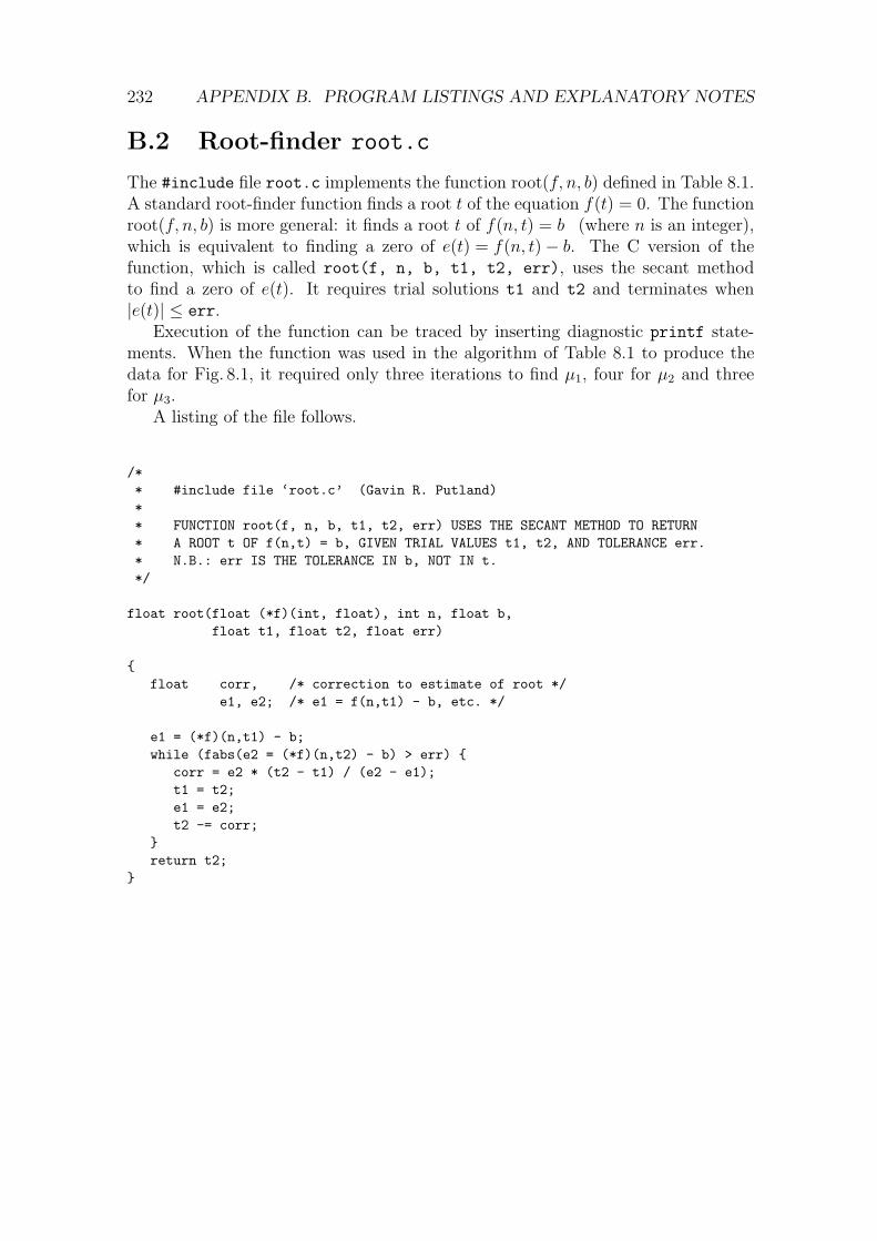
232 APPENDIX B. PROGRAM LISTINGS AND EXPLANATORY NOTES
B.2 Root-finder root.c
The #include file root.c implements the function root(f, n, b) defined in Table 8.1.A standard root-finder function finds a root t of the equation f(t) = 0. The functionroot(f, n, b) is more general: it finds a root t of f(n, t) = b (where n is an integer),which is equivalent to finding a zero of e(t) = f(n, t)− b. The C version of thefunction, which is called root(f, n, b, t1, t2, err), uses the secant methodto find a zero of e(t). It requires trial solutions t1 and t2 and terminates when|e(t)| ≤ err.
Execution of the function can be traced by inserting diagnostic printf state-ments. When the function was used in the algorithm of Table 8.1 to produce thedata for Fig. 8.1, it required only three iterations to find µ1, four for µ2 and threefor µ3.
A listing of the file follows.
/** #include file ‘root.c’ (Gavin R. Putland)** FUNCTION root(f, n, b, t1, t2, err) USES THE SECANT METHOD TO RETURN* A ROOT t OF f(n,t) = b, GIVEN TRIAL VALUES t1, t2, AND TOLERANCE err.* N.B.: err IS THE TOLERANCE IN b, NOT IN t.*/
float root(float (*f)(int, float), int n, float b,float t1, float t2, float err)
float corr, /* correction to estimate of root */
e1, e2; /* e1 = f(n,t1) - b, etc. */
e1 = (*f)(n,t1) - b;while (fabs(e2 = (*f)(n,t2) - b) > err)
corr = e2 * (t2 - t1) / (e2 - e1);t1 = t2;e1 = e2;t2 -= corr;
return t2;

B.3. EIGENFUNCTION PLOTTER EFUNC.C 233
B.3 Eigenfunction plotter efunc.c
Program efunc.c implements the algorithm of Table 8.1. It has numerical andgraphical printout options, either of which may be commented out. The graphicaloption produced the plotting commands for Fig. 8.1. Whereas the eigenfunctionsare computed with a step size of 0.01, the numerical and graphical printouts use x-increments of 0.5 and 0.1 respectively; this explains the instructions for incrementingi in the printing loops.
In the for loop that finds µn for n = 1 to 3, the root-finder function requirestwo estimates of µn for each n; these estimates are called t1 and t2. To initializethe loop, the second estimate of µ1 is found from Eq. (8.68). At the end of the loop,the second estimate of µn+1 is found from the final value of µn using Eq. (8.66). Foreach n, t1 is arbitrarily set to 99% of t2, so that t2 is the more accurate estimate(see the end of Subsection 8.2.4).
A listing of efunc.c follows.
/** Program ‘efunc.c’ (Gavin R. Putland)** PROGRAM TO FIND AND PLOT THE FIRST THREE EIGENFUNCTIONS OF THE* STURM-LIOUVILLE PROBLEM** y’’ + (1/x) y’ + mu^2 y = 0 (1)* y(1) = 0 (2)* y’(m) = 0 (3)** where mu is the eigenvalue and m is given. As a normalizing condition,* we will take** y’(1) = 1. (4)** STRATEGY FOR FINDING THE nth EIGENVALUE mu[n]: Take two trial* values of mu. For each trial value, solve the initial value problem* (1), (2), (4) for s(n,mu), the abscissa of the nth stationary point* of y(x). Use the secant method to find further trial values of mu,* making s(n,mu) converge to m.** CONTENTS OF #include FILE ‘stepstat.c’:** Function s(n,mu) returns the abscissa of the nth stationary point.* It repeatedly calls function step(mu), which is defined first.* step(mu) performs one step of the IVP solution for given mu.* Global array declarations are included.** CONTENTS OF #include FILE ‘root.c’:** Function root(f, n, b, t1, t2, err) uses the secant method to return* a root t of f(n,t) = b, given trial values t1, t2, and tolerance err.* N.B.: err is the tolerance in b, NOT in t.*/
#include <stdio.h>#include <math.h>

234 APPENDIX B. PROGRAM LISTINGS AND EXPLANATORY NOTES
#define pi 3.141592654F
#define m 20.F /* desired abscissa of stationary point of y(x) */#define tol 0.00001F /* tolerance to which s(n,mu) must match m */#define max 2500 /* maximum number of steps; must be > (m-1)/h */#define h 0.01F /* step size for IVP solution */
#include "stepstat.c" /* IVP solver, stationary point finder,array declarations */
#include "root.c" /* secant-method root finder */
main()
float mu[4], /* eigenvalues of mu; mu = mu[n] makes s(n,mu) = m,where s(n,mu) is the abscissa of thenth stationary point of y(x). */
t1, t2, /* initial estimates of eigenvalue */Y[4][max]; /* eigenfunctions; called y1, y2 and y3 in printout */
int n, /* index to eigenvalues and eigenfunctions */steps; /* number of steps from x=1 to x=m */
steps = (int)((m - 1.F)/h + 0.1F);
/* Initialize loop using ‘‘rough’’ analytical estimate of mu[1]: */t2 = 1.0 / sqrt(0.5 * (m*m - 1.F) * log(0.5 * (m + 1.F)));
for (n = 1; n <= 3; n++) /* FIND mu[n] AND COPY EIGENFUNCTION Y[n][i]: */ t1 = 0.99F * t2;mu[n] = root(s, n, m, t1, t2, tol);for (i = 0; i <= steps; i++)
Y[n][i] = (float)y[i];t2 = mu[n] + pi/(m - 1.F); /* add a half-cycle; mu <=> wave number */
/*NUMERICAL PRINTOUT OPTION:
*/
printf("\n mu1 = %7.5f ; mu2 = %7.5f ; mu3 = %7.5f .\n",mu[1], mu[2], mu[3]);
printf("\n %4s %6s %6s %6s\n\n", "x ", "y1 ", "y2 ", "y3 ");
for (i = 0; i <= steps; i += (int)(0.5F/h + 0.1F))printf(" %4.1f %6.3f %6.3f %6.3f\n",
x[i], Y[1][i], Y[2][i], Y[3][i]);
printf("\n");
/*GRAPHICAL PRINTOUT OPTION:
This option produces LaTeX picture commands to plot points in the threeeigenfunctions and the limiting function y = ln x (for mu = 0). The outputshould be redirected to a file and inserted in another file containingthe rest of the picture environment, including the axes and labels. The

B.3. EIGENFUNCTION PLOTTER EFUNC.C 235
output also includes a comment listing the eigenvalues.
printf("%% mu1 = %7.5f ; mu2 = %7.5f ; mu3 = %7.5f .\n",mu[1], mu[2], mu[3]);
for (i = 0; i <= steps; i++)Y[0][i] = (float)log(x[i]);
for (i = 0; i <= steps; i += (int)(0.1F/h + 0.1F)) printf("\\put(%4.0f,%4.0f)\\circle*1 ", 60*x[i], 180*Y[0][i]);printf("\\put(%4.0f,%4.0f)\\circle*1\n", 60*x[i], 180*Y[1][i]);printf("\\put(%4.0f,%4.0f)\\circle*1 ", 60*x[i], 180*Y[2][i]);printf("\\put(%4.0f,%4.0f)\\circle*1\n", 60*x[i], 180*Y[3][i]);
*/

236 APPENDIX B. PROGRAM LISTINGS AND EXPLANATORY NOTES
B.4 Program chase.c: Check results of Chase.
Program chase.c implements the algorithm of Table 8.2 and prints Table 8.3. Whenthe program efunc.c has been understood, the following listing of chase.c is self-explanatory.
/** Program ‘chase.c’ (Gavin R. Putland)** PROGRAM TO CHECK VALUES OF m USED BY CHASE** Unless otherwise noted, the nomenclature of program ‘efunc.c’ is used.*** CONTENTS OF #include FILE ‘stepstat.c’:** Function s(n,mu) returns the abscissa of the nth stationary point.* It repeatedly calls function step(mu), which is defined first.* step(mu) performs one step of the IVP solution for given mu.* Global array declarations are included.** CONTENTS OF #include FILE ‘root.c’:** Function root(f, n, b, t1, t2, err) uses the secant method to return* a root t of f(n,t) = b, given trial values t1, t2, and tolerance err.* N.B.: err is the tolerance in b, NOT in t.*/
#include <stdio.h>#include <math.h>
#define h 0.01F /* step size */#define max 2500 /* maximum number of steps; must be > (m-1)/h */#define tol 0.00001F /* tolerance to which s(1,mu) must match m */
#define rof 2400.F /* density of glass, kg/m^3 */#define a 5e-6F /* fibre radius, metres */#define alpha 1.87e-5F /* Chase’s thermal diffusivity of air, m^2/s */
#include "stepstat.c" /* IVP solver, stationary point finder,array declarations */
#include "root.c" /* secant-method root finder */
void check(float rom, float wc)
/** FUNCTION check(rom, wc) REPORTS ON THE POINT (rom, wc)* FROM CHASE’S FIGURE 1.*/
float m, much, t1, t2, muhalfm;
m = sqrt(rof/rom); /* m according to density */much = a * m * sqrt(wc/alpha); /* eigenvalue used by Chase */
/* COMPUTE EIGENVALUE FOR VALUE OF m APPARENTLY USED BY CHASE: */

B.4. PROGRAM CHASE.C: CHECK RESULTS OF CHASE. 237
m /= 2.F; /* Chase gets eigenvalue from m/2 instead of m ?? */t2 = 1.0 / sqrt(0.5 * (m*m - 1.F) * log(0.5 * (m + 1.F)));t1 = 0.99F * t2;muhalfm = root(s, 1, m, t1, t2, tol);m *= 2.F; /* restore m */
printf(" %4.1f %4.0f %5.2f %6.4f %6.4f\n",rom, wc, m, much, muhalfm);
main()
float rom, /* packing density of fibre = f * rof */wc; /* transition angular frequency = 1/tau */
/* PRINT HEADING: */printf("\n CHECK ON EIGENVALUES USED BY CHASE\n");printf("\n %4s %4s %5s %6s %7s\n\n",
"rom ", "wc ", "m ", "much ", "muhalfm");
/* PROCESS VALUES FROM CHASE’S FIGURE 1: */check(6.0F, 22.F);check(7.1F, 30.F);check(10.F, 67.F);check(20.F, 430.F);check(30.F, 1100.F);check(49.F, 3000.F);check(70.F, 5400.F);
printf("\n");

238 APPENDIX B. PROGRAM LISTINGS AND EXPLANATORY NOTES
B.5 Program f2.c: Locate 2nd-mode heatshed.
The program f2.c produces the output shown in Table 8.4. It uses the algorithmdescribed in Subsection 8.2.6, except that the body of the loop headed “For eachm” is relegated to the function printrow(m). The values of m are chosen so that mcan approach both unity and infinity while assuming “round-figure” values. (Similarsequences also occur in the program mu.c, to be described in the next section.)
The root-finder function requires two estimates of µ2. The more accurate esti-mate, called t2, is obtained from Eqs. (8.68) and (8.66); see the comments in thefunction printrow(m).
The source file for f2.c is listed below.
/** Program ‘f2.c’ (Gavin R. Putland)** FOR A RANGE OF VALUES OF m, FIND THE FRACTION OF THE AIR VOLUME* THAT CAN EXCHANGE HEAT WITH THE FIBRE IN THE SECOND MODE,* i.e. THE FRACTION OF THE AIR CROSS-SECTIONAL AREA INSIDE THE FIRST* MAXIMUM OF THE SECOND EIGENFUNCTION.** m AND mu ARE AS DEFINED IN PROGRAM ‘efunc.c’.** CONTENTS OF #include FILE ‘stepstat.c’:** Function s(n,mu) returns the abscissa of the nth stationary point.* It repeatedly calls function step(mu), which is defined first.* step(mu) performs one step of the IVP solution for given mu.* Global arrays and the global array index are declared.** CONTENTS OF #include FILE ‘root.c’:** Function root(f, n, b, t1, t2, err) uses the secant method to return* a root t of f(n,t) = b, given trial values t1, t2, and tolerance err.* N.B.: err is the tolerance in b, NOT in t.*/
#include <stdio.h>#include <math.h>
#define min(A,B) ((A)<(B)?(A):(B))
#define pi 3.141592654F
#define max 9000 /* maximum number of steps; must be > (m-1)/h */
float h; /* step size for #included functions */
#include "stepstat.c" /* IVP solver, stationary point finder,array & array index declarations */
#include "root.c" /* secant-method root finder */
void printrow(float m)
/** FUNCTION printrow(m) PROCESSES ONE VALUE OF m

B.5. PROGRAM F2.C: LOCATE 2ND-MODE HEATSHED. 239
* AND PRINTS A ROW OF OUTPUT.*/
float
f, /* filling factor */mu2, /* second eigenvalue */t1, t2, /* initial estimates of mu2 */tol, /* tolerance to which s(2,mu) must match m */f2; /* volume fraction inside s(1,mu2) */
/* Find filling factor: */f = 1.F / (m * m);
/* Initialize root-finder using rough analytical estimate of mu1... */t2 = 1.0 / sqrt(0.5 * (m*m - 1.F) * log(0.5 * (m + 1.F)));
/* ...followed by estimated difference between eigenvalues: */t2 += pi / (m - 1.F);t1 = 0.99F * t2;
/* Find mu2 and f2: */tol = m * 2e-7F;h = min(0.02F,(m - 1.F)/100.F);mu2 = root(s, 2, m, t1, t2, tol);f2 = (float)(pow(s(1,mu2),2)-1.0) / (m*m - 1.F);
printf("%6.3f %6.2f %9.5f %6.3f\n",1e2*f, m, mu2, 1e2*f2);
main()
float m; /* normalized variable related to filling factorand appearing in Sturm-Liouville problem */
/* HEADING OF PRINTOUT: */printf("\n%6s %6s %9s %6s\n\n",
"f(%) ", "m ", "mu2 ", "f2(%)");
for (m = 160.F; m > 3.F; m /= 1.414213562F)printrow(m);
printf("\n");
for (m = 2.28F; m > 1.009F; m -= 0.5F * (m - 1.F))printrow(m);
printf("\n");

240 APPENDIX B. PROGRAM LISTINGS AND EXPLANATORY NOTES
B.6 Program mu.c: Check eigenvalue approxima-tions.
Program mu.c implements the algorithm of Table 8.5, with some refinements men-tioned in the text of Subsection 8.2.7. When zeta is defined as 0.37, the programproduces the output shown in Table 8.6.
The listing follows.
/** Program ‘mu.c’ (Gavin R. Putland)** FIND THE FIRST EIGENVALUE OF mu IN THE STURM-LIOUVILLE PROBLEM** y’’ + (1/x) y’ + mu^2 y = 0 (1)* y(1) = 0 (2)* y’(m) = 0 (3)** FOR A RANGE OF VALUES OF m, AND COMPARE THE EIGENVALUE WITH TWO* ANALYTICAL ESTIMATES THEREOF.** As a normalizing condition we will take** y’(1) = 1. (4)** STRATEGY FOR FINDING THE 1st EIGENVALUE mu1: Take two trial* values of mu. For each trial value, solve the initial value problem* (1), (2), (4) for s(1,mu), the abscissa of the 1st stationary point* of y(x). Use the secant method to find further trial values of mu,* making s(1,mu) converge to m.** CONTENTS OF #include FILE ‘stepstat.c’:** Function s(n,mu) returns the abscissa of the nth stationary point.* It repeatedly calls function step(mu), which is defined first.* step(mu) performs one step of the IVP solution for given mu.* Global arrays and the global array index are declared.** CONTENTS OF #include FILE ‘root.c’:** Function root(f, n, b, t1, t2, err) uses the secant method to return* a root t of f(n,t) = b, given trial values t1, t2, and tolerance err.* N.B.: err is the tolerance in b, NOT in t.*/
#include <stdio.h>#include <math.h>
#define min(A,B) ((A)<(B)?(A):(B))
#define max 9000 /* maximum number of steps; must be > (m-1)/h */#define zeta 0.37 /* parameter in ‘‘refined’’ analytical approx. */
float h; /* step size for #included functions */
#include "stepstat.c" /* IVP solver, stationary point finder,

B.6. PROGRAM MU.C: CHECK EIGENVALUE APPROXIMATIONS. 241
array & array index declarations */#include "root.c" /* secant-method root finder */
void printrow(float m)
/** FUNCTION printrow(m) PROCESSES ONE VALUE OF m* AND PRINTS A ROW OF OUTPUT.*/
float
f, /* filling factor */mu1, /* first eigenvalue (computed from smaller h) */mu1d, /* first eigenvalue (computed from larger h) */t1, t2, /* initial estimates of eigenvalue */tol, /* tolerance to which s(1,mu) must match m */errmu, /* difference between mu1 and mu1d (in ppm) */mua, mub, /* analytical estimates of mu1 (from m) */ermua, ermub; /* percentage errors in mua and mub */
/* Find filling factor: */f = 1.F / (m * m);
/* Initialize root-finder using ‘‘rough’’ analytical estimate of mu1: */t2 = 1.0 / sqrt(0.5 * (m*m - 1.F) * log(0.5 * (m + 1.F)));t1 = 0.99F * t2;
/* Find eigenvalue using two step sizes and estimate error: */tol = m * 1e-7F;h = min(0.02F,(m - 1.F)/100.F);mu1d = root(s, 1, m, t1, t2, tol);h /= 2.F;mu1 = root(s, 1, m, t1, t2, tol);errmu = 1e6F * (mu1d - mu1) / mu1;
/* Find ‘‘rough’’ and ‘‘refined’’ analytical estimates & their errors: */mua = t2;mub = 1.0 / sqrt(0.5 * (m*m - pow(m,zeta)) * log(0.5 * (m + 1.F)));ermua = 100.F * (mua - mu1) / mu1;ermub = 100.F * (mub - mu1) / mu1;
printf("%9.3f %5.2f %9.6f %5i %6.2f %5.2f %5.2f\n",1e2*f, m, mu1, i, errmu, ermua, ermub);
main()
float m; /* normalized variable related to filling factorand appearing in Sturm-Liouville problem */
/* HEADING OF PRINTOUT: */printf("\n%9s %5s %9s %5s %6s %5s %5s\n\n",
"f(%) ", "m ", "mu1 ", "steps", "errmu", "ermua", "ermub");
for (m = 80.F; m > 3.F; m /= 1.414213562F)printrow(m);
printf("\n");

242 APPENDIX B. PROGRAM LISTINGS AND EXPLANATORY NOTES
for (m = 2.28F; m > 1.019F; m -= 0.5F * (m - 1.F))printrow(m);
printf("\n");

B.7. PROGRAM TAFP.C: TABULATE THERMAL TIME CONSTANT τFP . 243
B.7 Program tafp.c: Tabulate thermal time con-stant τfp.
Program tafp.c estimates thermal time constants using Eq. (8.16), with ζ = 0.37.It also uses some acoustical properties of air, which are calculated using the formulaeof Chapter 9. Its output is shown in Table 8.7.
The listing follows.
/** Program ‘tafp.c’ (Gavin R. Putland)** PROGRAM TO COMPUTE THE THERMAL TIME CONSTANT tafp* FOR VARIOUS VALUES OF FILLING FACTOR f AND FIBRE DIAMETER d* USING THE ‘‘REFINED’’ ANALYTICAL FORMULA FROM PROGRAM ‘tau.c’,* WITH zeta = 0.37.*/
#include <stdio.h>#include <math.h>
#define pi 3.141592654F#define Rbar 8.31451F /* universal gas constant, J/(K.mol) */#define mbar 0.028964F /* molecular mass of air, kg/mol */#define Cp 1007.F /* Cp of air, J/(kg.K) */#define Po 101325.F /* atmospheric pressure, Pa */#define T 293.15F /* ambient temperature, K */
floatd, /* fibre diameter, metres (um in printout) */f, /* filling factor (percent in printout) */m, /* m = 1/sqrt(f) */mfac, /* m-dependent factor in expression for tafp */tafp, /* time constant, seconds (usec in printout) */
/* PROPERTIES OF AIR: */rho, /* density, kg/m^3 */kappa, /* thermal conductivity, W/(m.K) */alpha; /* thermal diffusivity, m^2/s */
main()
/* COMPUTE PROPERTIES OF AIR: */rho = Po * mbar / (Rbar * T);kappa = 0.02623 * pow((T/300.F),0.851);alpha = kappa / (rho * Cp);
/* HEADING OF PRINTOUT: */printf("\n T = %6.2f K; Po = %6.0f Pa.\n", T, Po);printf("\n rho = %5.3f; kappa = %7.5f; alpha = %8.3e (SI units).\n",
rho, kappa, alpha);printf("\n THERMAL TIME CONSTANT tafp (IN MICROSECONDS)");printf("\n vs. FILLING FACTOR f AND FIBRE DIAMETER d:\n");printf("\n %6s", "d(um):");for (d = 4e-6; d < 17e-6; d += 2e-6)
printf(" %2.0f ", 1e6*d);

244 APPENDIX B. PROGRAM LISTINGS AND EXPLANATORY NOTES
printf("\n\n %4s\n", "f(%)");
/* COMPUTE AND PRINT VALUES OF tafp: */for (f = 0.0005; f < 0.0901; /* f is incremented at end of loop */ )
m = 1.0 / sqrt(f);mfac = (m*m - pow(m,0.37)) * log(0.5 * (m + 1.0));printf(" %4.2f ", 1e2*f);for (d = 4e-6; d < 17e-6; d += 2e-6)
tafp = d * d * mfac / (8.F * alpha);printf(" %7.2f", 1e6*tafp);
printf("\n");/* INCREMENT f: */
if (f < 0.0049)f += 0.0005;
else if (f < 0.0099)f += 0.001;
else if (f < 0.0199)f += 0.002;
else if (f < 0.0499)f += 0.005;
elsef += 0.01;
printf("\n");

B.8. PROGRAM AIR.C: TABULATE ACOUSTICAL PROPERTIES OF AIR.245
B.8 Program air.c: Tabulate acoustical proper-ties of air.
The program air.c, listed below, is a straightforward application of the formulaedeveloped in Chapter 9. It produces the output shown in Table 9.1.
/** Program ‘air.c’ (Gavin R. Putland)* ACOUSTICAL PROPERTIES OF AIR vs. TEMPERATURE AND PRESSURE*/
#include <stdio.h>#include <math.h>
#define Rbar 8.31451F /* universal gas constant, J/(K.mol) */#define mbar 0.028964F /* molecular mass of air, kg/mol */#define Cp 1007.F /* Cp of air, J/(kg.K) */
float gam, T, Po, rho, c, rhoc, eta, kappa, alpha;
void printline(void)
/* FUNCTION TO COMPUTE & PRINT ONE LINE OF OUTPUT: */
rho = Po * mbar / (Rbar * T); /* density, kg/m^3 */c = sqrt(gam * Rbar * T / mbar); /* speed of sound, m/s */rhoc = rho * c; /* impedance, Pa s/m */eta = 1.857e-5 * pow((T/300.F),0.7829); /* viscosity, Pa s */kappa = 0.02623 * pow((T/300.F),0.851); /* conductivity, W/(m.K) */alpha = kappa / (rho * Cp); /* diffusivity, m^2/s */printf("%6.2f %6.0f %7.5f %6.2f %6.2f %9.3e %7.5f %8.2e\n",
T, Po, rho, c, rhoc, eta, kappa, alpha);
main()
gam = Cp / (Cp - Rbar/mbar); /* ratio of specific heats */
/* HEADING OF PRINTOUT: */printf("\n");printf("ACOUSTICAL PROPERTIES OF AIR vs. TEMPERATURE AND PRESSURE\n\n");printf("All units are SI.\n\n");printf("Rbar = %7.5f ; mbar = %8.6f ; Cp = %4.0f ; gamma = %6.4f .\n\n",
Rbar, mbar, Cp, gam);printf("%6s %6s %7s %6s %6s %9s %7s %8s\n\n",
"T ","Po ","rho ","c ","rhoc ","eta ","kappa ","alpha ");
Po = 101325.F; /* atmospheric pressure, Pa */
for (T = 200.F; T < 405.F; T += 50.F) /* fixed Po */printline();
printf("\n");

246 APPENDIX B. PROGRAM LISTINGS AND EXPLANATORY NOTES
for (T = 273.15F; T < 305.F; T += 5.F) /* fixed Po */printline();
printf("\n");
/* U.S. Standard Atmosphere sequence (variable Po): */T = 307.659F; Po = 142970.F; printline();T = 297.902F; Po = 120690.F; printline();T = 288.150F; Po = 101325.F; printline();T = 278.402F; Po = 84559.F; printline();T = 268.659F; Po = 70121.F; printline();T = 258.921F; Po = 57752.F; printline();T = 249.187F; Po = 47217.F; printline();
printf("\n");
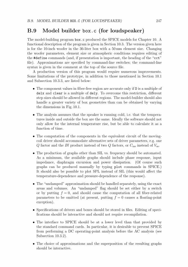
B.9. MODEL BUILDER BOX.C (FOR LOUDSPEAKER) 247
B.9 Model builder box.c (for loudspeaker)
The model-building program box.c produced the SPICE models for Chapter 10. Afunctional description of the program is given in Section 10.3. The version given hereis for the 10-inch woofer in the 36-liter box with a 50mm element size. Changingthe woofer parameters, element size or atmospheric conditions requires editing ofthe #define commands (and, if presentation is important, the heading of the “cct”file). Approximations are specified by command-line switches; the command-linesyntax is given in the comment at the top of the source file.
A production version of this program would require numerous improvements.Some limitations of the prototype, in addition to those mentioned in Section 10.1and Subsection 10.3.3, are listed below:
• The component values in fiber-free region are accurate only if D is a multiple ofdelx and clear is a multiple of dely. To overcome this restriction, differentstep sizes should be allowed in different regions. The model-builder should alsohandle a greater variety of box geometries than can be obtained by varyingthe dimensions in Fig. 10.1.
• The analysis assumes that the speaker is running cold, i.e. that the tempera-tures inside and outside the box are the same. Ideally the software should notonly allow for the internal temperature rise, but be able to calculate it as afunction of time.
• The computation of the components in the equivalent circuit of the moving-coil driver should accommodate alternative sets of driver parameters, e.g. oneQ factor and the Bl product instead of two Q factors, or Cms instead of Vas.
• The production of graphs other than SIL vs. frequency should be automated.As a minimum, the available graphs should include phase response, inputimpedance, diaphragm excursion and power dissipation. (Of course suchgraphs can be produced manually by typing plot commands in SPICE.)It should also be possible to plot SPL instead of SIL (this would affect thetemperature-dependence and pressure-dependence of the response).
• The “undamped” approximation should be handled separately, using the exactareas and volumes. An “undamped” flag should be set either by a switchor by putting f = 0, and should cause the computation of all fiber-relatedparameters to be omitted (at present, putting f = 0 causes a floating-pointexception).
• Specifications of drivers and boxes should be stored in files. Editing of speci-fications should be interactive and should not require recompilation.
• The interface to SPICE should be at a lower level than that provided bythe standard command cards. In particular, it is desirable to prevent SPICEfrom performing a DC operating-point analysis before the AC analysis (seeSubsection 10.3.2).
• The choice of approximations and the superposition of the resulting graphsshould be interactive.

248 APPENDIX B. PROGRAM LISTINGS AND EXPLANATORY NOTES
The source file box.c follows.
/*********************************************************************************************************************************************************
PROGRAM box.c (GAVIN R. PUTLAND)CALCULATION OF SOUND INTENSITY LEVEL VS. FREQUENCY AT ONE METRE.Box interior is modeled as lumped compliance or 2D network.SPICE3 CIRCUIT DEFINITION IS WRITTEN TO FILE ‘cct’.SPICE3 COMMAND SCRIPT IS WRITTEN TO FILE ‘go’.
USAGE (assuming executable file is called ‘box’):
box outfilebox -l outfilebox -[f|s|u][a|n|e] outfile
where outfile is the name of the file to which the frequency responsevector is written (in the SPICE3 command script). With no switches, boxdoes a full simulation. The switches denote the following approximationconditions:
l lumped lumped-compliance box model; no fibref free no resistance to air motion (HF)s stiff fibre matrix is stiff (HF)u unison fibre moves with air (LF)a adiab adiabatic compression (HF)n nearad near-adiabatic, delCth shorted (HF)e equil thermal equilibrium (LF)
Actually any combination of the above switches is accepted, but ‘l’renders all others superfluous. Among the other switches, the followingpecking orders apply: f>s>u and a>n>e.
*********************************************************************************************************************************************************/
#include <stdio.h>#include <math.h>#include <string.h>
/*****************DEFINITIONS:
*****************/
/* CONSTANTS: */#define pi 3.141592654F
/* FIXED PROPERTIES OF AIR: */#define Rbar 8.31451F /* universal gas constant, J/(K.mol) */#define mbar 0.028964F /* molecular mass of air, kg/mol */#define Cp 1007.F /* Cp of air, J/(kg.K) */
/* AMBIENT CONDITIONS: */#define T 293.15F /* absolute temperature, K */#define Po 101325.F /* pressure, Pa */
/* GIVEN DRIVER PARAMETERS (ALTRONICS C3065 10-INCH WOOFER): */

B.9. MODEL BUILDER BOX.C (FOR LOUDSPEAKER) 249
#define fs 35.F /* free air resonance, Hz */#define Qts 0.4224F#define Qms 2.26F#define Vas 0.0774F /* suspension equiv. volume, m^3 */#define Re 7.F /* approx. voice coil resistance, ohms */#define D 0.25F /* overall diameter, metres */#define a 0.1F /* diaphragm radius, metres */
/* SIMULATION CONDITIONS: */#define Vg 2.828427125F /* rms voltage for 1W into 8 ohms */#define fbot 10.F /* bottom frequency of AC plot */#define ftop 10000.F /* top frequency of AC plot */#define del 0.05F /* min. vol. element size, metres */
/* BOX INTERIOR DIMENSIONS, metres: */#define width 0.25F#define depth 0.3F#define height 0.6F#define clear 0.1F /* fibre-free clearance behind driver */
/* SPECIFICATIONS OF FIBRE FILLING: */#define d 10e-6F /* diameter, metres */#define f 0.0025F /* filling factor */#define rof 2400.F /* intrinsic density, kg/m^3 */#define Cf 670.F /* specific heat, J/(kg.K) */
/************************EXTERNAL VARIABLES:
************************/
/* FILE POINTERS TO SPICE3 CIRCUIT DEFINITION AND COMMAND SCRIPT: */FILE *cct, *go;
/* FILE NAME FOR FREQUENCY RESPONSE VECTOR (SPICE3 OUTPUT): */char outfile[32];
/* COUNTS AND COUNTERS: */int nhor, nvert, /* network dimensions */
nclear, /* no. clear elements behind driver (horizontally) */split, /* no. clear elements behind driver (vertically) */i, j, k; /* horizontal & vertical indices and node number */
/* REAL VARIABLES (commented in main): */float gam, roo, c, eta, kappa, alpha, ws, Qes, Cas, Ras, Mas, G,
Mar, Rar, Pro, Mad, lambda, beta, m, tafp, delx, dely,delMx, delMy, delMxa, delRx, delMxf, delMya, delRy, delMyf,delC, delCa, delRth, delCth, Mab, delRxs, Rleak, Vab, Cab;
main(int argc, char *argv[])
/* APPROXIMATION CONDITIONS (from command-line switches): */int lumped = 0, /* lumped-compliance box model; no fibre */
free = 0, /* no resistance to air motion (HF) */stiff = 0, /* fibre matrix is stiff (HF) */unison = 0, /* fibre moves with air (LF) */adiab = 0, /* adiabatic compression (HF) */

250 APPENDIX B. PROGRAM LISTINGS AND EXPLANATORY NOTES
nearad = 0, /* near-adiabatic, delCth shorted (HF) */equil = 0; /* thermal equilibrium (LF) */
/************************************PROCESS COMMAND LINE ARGUMENTS:
************************************/
/* CHECK FOR ILLEGAL ARGUMENTS: */
if (argc < 2) fprintf(stderr, "Too few arguments.\n");exit(1);
if (argc > 3)
fprintf(stderr, "Too many arguments.\n");exit(1);
if (argc == 2 && *(argv[1]) == ’-’)
fprintf(stderr, "You can’t start filename with minus sign.\n");exit(1);
if (argc == 3 && *(argv[2]) == ’-’)
fprintf(stderr, "You can’t start filename with minus sign.\n");exit(1);
if (argc == 3 && *(argv[1]) != ’-’)
fprintf(stderr, "Switch(es) must follow single minus sign.\n");exit(1);
/* SET FLAGS AND SPICE3 OUTPUT FILE NAME: */
if (argc == 2)strcpy(outfile, argv[1]);
if (argc == 3) strcpy(outfile, argv[2]);while (i = *++argv[1]) /* while i is not null character */
switch (i) case ’l’:
lumped = 1;break;
case ’f’:free = 1;break;
case ’s’:stiff = 1;break;
case ’u’:unison = 1;break;
case ’a’:adiab = 1;break;
case ’n’:nearad = 1;break;
case ’e’:

B.9. MODEL BUILDER BOX.C (FOR LOUDSPEAKER) 251
equil = 1;break;
default:fprintf(stderr, "Illegal switch \’%c\’.\n", i);exit(1);
/***********************************EQUIVALENT CIRCUIT COMPONENTS:
***********************************/
/* DERIVED ACOUSTICAL PROPERTIES OF AIR: */gam = Cp / (Cp - Rbar/mbar); /* gamma (constant) */roo = Po * mbar / (Rbar * T); /* density, kg/m^3 */c = sqrt(gam * Rbar * T / mbar); /* speed of sound, m/s */eta = 1.857e-5 * pow((T/300.F),0.7829); /* viscosity, Pa s */kappa = 0.02623 * pow((T/300.F),0.851); /* conductivity, W/(m.K) */alpha = kappa / (roo * Cp); /* diffusivity, m^2/s */
/* DERIVED DRIVER PARAMETERS: */ws = 2.0 * pi * fs;Qes = 1 / (1/Qts - 1/Qms);Cas = Vas / (gam * Po);Ras = 1/(ws * Cas * Qms);Mas = 1/(Cas * ws * ws);G = sqrt(Qes * ws * Cas / Re); /* driver gyrator ratio S/Bl */Mar = 8 * roo / (3 * pi * pi * a); /* radiation inertance */Rar = 128*roo*c/(9*pi*pi*pi*a*a); /* radiation resistance, parallel */Pro = sqrt(2e-12 * pi * Rar); /* O/P pressure for 0dB SIL at 1m
radiating into half-space *//* Driver inertance without free-air mass load,
assuming two-sided free-air load equals one-sided baffled air load: */Mad = Mas - Mar;
/* DERIVED FIBRE PARAMETERS: */lambda = 27.F * eta * (float)pow(f,1.4) / (d*d);beta = gam * f * rof * Cf / ((1.F - f) * roo * Cp);m = 1.0 / sqrt(f);tafp = d*d * (m*m - pow(m,0.37)) * log(0.5 * (m + 1.0)) / (8.F * alpha);
/* DERIVED BOX PARAMETERS: */nhor = (int)(depth/del + 0.01F);nvert = (int)(height/del + 0.01F);nclear = (int)(nhor*clear/depth + 0.5F);split = (int)(nvert*D/height + 0.5F); /* elements spanned by driver */delx = depth / nhor;dely = height / nvert;delMx = roo * delx / (width * dely); /* for undamped region */delMy = roo * dely / (width * delx); /* for undamped region */delMxa = delMx / (1.F - f);delRx = lambda * delMxa / roo;delMxf = f * rof * delMxa / ((1.F - f) * roo);delMya = delMy / (1.F - f);delRy = lambda * delMya / roo;delMyf = f * rof * delMya / ((1.F - f) * roo);

252 APPENDIX B. PROGRAM LISTINGS AND EXPLANATORY NOTES
delC = width * delx * dely / (gam * Po);delCa = (1.F - f) * delC;delRth = tafp / ((gam - 1.F) * delCa);delCth = (gam - 1.F) * beta * delCa / (gam + beta);Vab = width * (clear * D + (depth - clear) * height);Cab = Vab / (gam * Po);
/* Air load on back of driver, not included in FDM network: */Mab = roo * 0.5F * delx / (pi * a*a);
/* To prevent zero DC mesh resistances: */delRxs = delMx / 1000.F; /* giving ‘L/R’ = 1000 seconds */
/* To give every node a DC path to ground: */Rleak = 1000.F / Cas; /* giving ‘RC’ = 1000 seconds */
/***************************************************WRITE SPICE3 CIRCUIT DEFINITION TO FILE ‘cct’:
***************************************************/
cct = fopen("cct", "w");
/* HEADER: */fprintf(cct, "ALTRONICS C3065 10-INCH WOOFER IN SEALED BOX:\n\n");
/* COMMENTS: */fprintf(cct, "* Driver parameters:\n");fprintf(cct, " * fs = %6.1f Hz\n", fs);fprintf(cct, " * Qts = %6.4f\n", Qts);fprintf(cct, " * Qms = %6.4f\n", Qms);fprintf(cct, " * Qes = %6.4f\n", Qes);fprintf(cct, " * Vas = %6.1f litres\n", 1e3 * Vas);fprintf(cct, " * Re = %6.1f ohms\n", Re);fprintf(cct, " * D = %6.0f mm\n", 1e3F * D);fprintf(cct, " * a = %6.0f mm\n", 1e3F * a);fprintf(cct, "* Box dimensions and divisions:\n");fprintf(cct, " * width = %4.0f mm\n", 1e3F * width);fprintf(cct, " * depth = %4.0f mm\n", 1e3F * depth);fprintf(cct, " * height = %4.0f mm\n", 1e3F * height);fprintf(cct, " * clear = %4.0f mm\n", 1e3F * clear);fprintf(cct, " * Vab = %6.4f m^3\n", Vab);fprintf(cct, " * delx = %6.0f mm\n", 1e3F * delx);fprintf(cct, " * dely = %6.0f mm\n", 1e3F * dely);fprintf(cct, " * nhor = %2i\n", nhor);fprintf(cct, " * nvert = %2i\n", nvert);fprintf(cct, " * nclear = %2i\n", nclear);fprintf(cct, " * split = %2i\n", split);fprintf(cct, "* Properties of air:\n");fprintf(cct, " * T = %6.2f K\n", T);fprintf(cct, " * Po = %6.0f Pa\n", Po);fprintf(cct, " * gam = %6.4f\n", gam);fprintf(cct, " * roo = %6.4f kg/m^3\n", roo);fprintf(cct, " * c = %6.2f m/s\n", c);fprintf(cct, "* Properties of fibre:\n");fprintf(cct, " * d = %6.0f um\n", 1e6F * d);fprintf(cct, " * f = %6.3f %%\n", 100.F * f);fprintf(cct, " * rof = %6.0f kg/m^3\n", rof);fprintf(cct, " * Cf = %6.0f J/(kg.K)\n", Cf);fprintf(cct, " * lambda = %4.0f Pa s/m^2\n", lambda);fprintf(cct, " * beta = %6.3f\n", beta);fprintf(cct, " * m = %6.3f\n", m);

B.9. MODEL BUILDER BOX.C (FOR LOUDSPEAKER) 253
fprintf(cct, " * tafp = %6.2f us\n", 1e6F * tafp);fprintf(cct, "* FDM component values:\n");fprintf(cct, " * delMx = %6.3f kg/m^4\n", delMx);fprintf(cct, " * delMxa = %6.3f kg/m^4\n", delMxa);fprintf(cct, " * delRx = %6.0f Pa s/m^3\n", delRx);fprintf(cct, " * delMxf = %6.3f kg/m^4\n", delMxf);fprintf(cct, " * delMy = %6.3f kg/m^4\n", delMy);fprintf(cct, " * delMya = %6.3f kg/m^4\n", delMya);fprintf(cct, " * delRy = %6.0f Pa s/m^3\n", delRy);fprintf(cct, " * delMyf = %6.3f kg/m^4\n", delMyf);fprintf(cct, " * delC = %6.3f mm^3/Pa\n", 1e9F * delC);fprintf(cct, " * delCa = %6.3f mm^3/Pa\n", 1e9F * delCa);fprintf(cct, " * delRth = %6.0f Pa s/m^3\n", delRth);fprintf(cct, " * delCth = %6.3f mm^3/Pa\n", 1e9F * delCth);fprintf(cct, "* Simulation specifications:\n");fprintf(cct, " * Vg = %6.3f V rms\n", Vg);fprintf(cct, " * fbot = %6.0f Hz\n", fbot);fprintf(cct, " * ftop = %6.0f Hz\n", ftop);fprintf(cct, " * Pro = %6.1f uPa\n", 1e6 * Pro);fprintf(cct, "\n");
/* DEFINE LUMPED COMPONENTS: */fprintf(cct, "* LUMPED COMPONENTS:\n\n");fprintf(cct, "Vg 1 0 dc 0 ac %f\n", Vg);fprintf(cct, "Re 1 2 %e\n", Re);fprintf(cct, "Lar 0 3 %e\n", Mar);fprintf(cct, "Rar 0 3 %e\n", Rar);fprintf(cct, "Cas 3 4 %e\n", Cas);fprintf(cct, "Rlk 3 4 %e\n", Rleak); /* DC path to ground */fprintf(cct, "Ras 4 5 %e\n", Ras);if (lumped)
fprintf(cct, "Lad 5 6 %e\n", Mas); /* with back air load */fprintf(cct, "Cab 7 0 %e\n", Cab); /* lumped box compliance */fprintf(cct, "Gf 7 6 2 0 %e\n", G);fprintf(cct, "Gb 2 0 6 7 %e\n", G);
else fprintf(cct, "Lad 5 6 %e\n", Mad + Mab); /* with FDM back air load *//* Box compliance and gyrator elements are not lumped;
see next heading. */fprintf(cct, "\n");
/* IF NOT ‘lumped’ APPROXIMATION: **************************************/
if (!lumped)
/* DEFINE SPLIT TRANSCONDUCTANCE: */fprintf(cct, "* SPLIT TRANSCONDUCTANCE:\n\n");/* SPLIT FORWARD TRANSCONDUCTANCE: */
for (j=0; j<split; j++)fprintf(cct, "Gf%.2i %3i 6 2 0 %e\n", j, 7+j, G/(float)split);
/* SPLIT BACKWARD TRANSCONDUCTANCE: */for (j=0; j<split; j++)
fprintf(cct, "Gb%.2i 2 0 6 %3i %e\n", j, 7+j, G/(float)split);fprintf(cct, "\n");
/* DEFINE INERTANCE SUBCIRCUITS *//* No series resistance needed for y element. */

254 APPENDIX B. PROGRAM LISTINGS AND EXPLANATORY NOTES
/* ‘Mxb’ is on boundary between fibre-filled and fibre-free regions. */fprintf(cct, "* MASS ELEMENT SUBCIRCUITS:\n\n");/* ‘UNDAMPED’ HORIZONTAL MASS ELEMENT: */
fprintf(cct, ".subckt Mxclearsub 1 3\n");fprintf(cct, "Lx 1 2 %e\n", delMx);fprintf(cct, "Rxs 2 3 %e\n", delRxs);fprintf(cct, ".ends Mxclearsub\n\n");
if (free) fprintf(cct, ".subckt Mxsub 1 3\n");fprintf(cct, "Lx 1 2 %e\n", delMxa);fprintf(cct, "Rxs 2 3 %e\n", delRxs);fprintf(cct, ".ends Mxsub\n\n");fprintf(cct, ".subckt Mysub 1 2\n");fprintf(cct, "Ly 1 2 %e\n", delMya);fprintf(cct, ".ends Mysub\n\n");fprintf(cct, ".subckt Mxbsub 1 3\n");fprintf(cct, "Lx 1 2 %e\n", 0.5F*(delMx + delMxa));fprintf(cct, "Rxs 2 3 %e\n", delRxs);fprintf(cct, ".ends Mxbsub\n\n");
else if (stiff) fprintf(cct, ".subckt Mxsub 1 3\n");fprintf(cct, "Lxa 1 2 %e\n", delMxa);fprintf(cct, "Rx 2 3 %e\n", delRx + delRxs);fprintf(cct, ".ends Mxsub\n\n");fprintf(cct, ".subckt Mysub 1 3\n");fprintf(cct, "Lya 1 2 %e\n", delMya);fprintf(cct, "Ry 2 3 %e\n", delRy);fprintf(cct, ".ends Mysub\n\n");fprintf(cct, ".subckt Mxbsub 1 3\n");fprintf(cct, "Lxa 1 2 %e\n", 0.5F*(delMx + delMxa));fprintf(cct, "Rx 2 3 %e\n", 0.5F*delRx + delRxs);fprintf(cct, ".ends Mxbsub\n\n");
else if (unison) fprintf(cct, ".subckt Mxsub 1 3\n");fprintf(cct, "Lx 1 2 %e\n", delMxa + delMxf);fprintf(cct, "Rxs 2 3 %e\n", delRxs);fprintf(cct, ".ends Mxsub\n\n");fprintf(cct, ".subckt Mysub 1 2\n");fprintf(cct, "Ly 1 2 %e\n", delMya + delMyf);fprintf(cct, ".ends Mysub\n\n");fprintf(cct, ".subckt Mxbsub 1 3\n");fprintf(cct, "Lx 1 2 %e\n", 0.5*(delMx + delMxa + delMxf));fprintf(cct, "Rxs 2 3 %e\n", delRxs);fprintf(cct, ".ends Mxbsub\n\n");
else /* if no approximation */ fprintf(cct, ".subckt Mxsub 1 4\n");fprintf(cct, "Lxa 1 2 %e\n", delMxa);fprintf(cct, "Rx 2 3 %e\n", delRx);fprintf(cct, "Lxf 2 3 %e\n", delMxf);fprintf(cct, "Rxs 3 4 %e\n", delRxs);fprintf(cct, ".ends Mxsub\n\n");fprintf(cct, ".subckt Mysub 1 3\n");fprintf(cct, "Lya 1 2 %e\n", delMya);fprintf(cct, "Ry 2 3 %e\n", delRy);fprintf(cct, "Lyf 2 3 %e\n", delMyf);fprintf(cct, ".ends Mysub\n\n");fprintf(cct, ".subckt Mxbsub 1 4\n");fprintf(cct, "Lxa 1 2 %e\n", 0.5*(delMx + delMxa));

B.9. MODEL BUILDER BOX.C (FOR LOUDSPEAKER) 255
fprintf(cct, "Rx 2 3 %e\n", 0.5*delRx);fprintf(cct, "Lxf 2 3 %e\n", 0.5*delMxf);fprintf(cct, "Rxs 3 4 %e\n", delRxs);fprintf(cct, ".ends Mxbsub\n\n");
/* DEFINE COMPLIANCE SUBCIRCUIT */fprintf(cct, "* COMPLIANCE ELEMENT SUBCIRCUIT:\n\n");if (adiab)
fprintf(cct, ".subckt Csub 1 2\n");fprintf(cct, "Ca 1 2 %e\n", delCa);fprintf(cct, ".ends Csub\n\n");
else if (nearad) fprintf(cct, ".subckt Csub 1 2\n");fprintf(cct, "Ca 1 2 %e\n", delCa);fprintf(cct, "Rth 1 2 %e\n", delRth);fprintf(cct, ".ends Csub\n\n");
else if (equil) fprintf(cct, ".subckt Csub 1 2\n");fprintf(cct, "C 1 2 %e\n", delCa + delCth);fprintf(cct, ".ends Csub\n\n");
else /* if no approximation */ fprintf(cct, ".subckt Csub 1 3\n");fprintf(cct, "Ca 1 3 %e\n", delCa);fprintf(cct, "Rth 1 2 %e\n", delRth);fprintf(cct, "Cth 2 3 %e\n", delCth);fprintf(cct, ".ends Csub\n\n");
/* WRITE UNDAMPED (CLEAR) COMPLIANCE ELEMENTS: */fprintf(cct, "* UNDAMPED (CLEAR) COMPLIANCE ELEMENTS:\n\n");for (i=0; i<nclear; i++)
for (j=0; j<split; j++) k = 7 + split*i + j;fprintf(cct, "C%.2i %2i 0 %e\n", k, k, delC);
fprintf(cct, "\n");
/* WRITE UNDAMPED (CLEAR) HORIZONTAL INERTANCE ELEMENTS: */fprintf(cct, "* UNDAMPED (CLEAR) HORIZONTAL INERTANCE ELEMENTS:\n\n");for (i=0; i<nclear-1; i++)
for (j=0; j<split; j++) k = 7 + split*i + j;fprintf(cct, "XLx%.2ito%.2i %2i %2i Mxclearsub\n",
k, k+split, k, k+split);
fprintf(cct, "\n");
/* WRITE UNDAMPED (CLEAR) VERTICAL INERTANCE ELEMENTS: */fprintf(cct, "* UNDAMPED (CLEAR) VERTICAL INERTANCE ELEMENTS:\n\n");for (i=0; i<nclear; i++)
for (j=0; j<split-1; j++) k = 7 + split*i + j;fprintf(cct, "Ly%.2ito%.2i %2i %2i %e\n",
k, k+1, k, k+1, delMy);
fprintf(cct, "\n");

256 APPENDIX B. PROGRAM LISTINGS AND EXPLANATORY NOTES
/* WRITE HALF-DAMPED HORIZONTAL INERTANCE ELEMENTS: */fprintf(cct, "* HALF-DAMPED HORIZONTAL INERTANCE ELEMENTS:\n\n");
i = nclear-1;for (j=0; j<split; j++)
k = 7 + split*i + j;fprintf(cct, "XLxb%.2i %2i %2i Mxbsub\n", j, k, k+split);
fprintf(cct, "\n");
/* WRITE DAMPED COMPLIANCE ELEMENTS: */fprintf(cct, "* DAMPED COMPLIANCE ELEMENTS:\n\n");for (i=nclear; i<nhor; i++)
for (j=0; j<nvert; j++) k = 7 + nclear*split + nvert*(i-nclear) + j;fprintf(cct, "XC%.3i %3i 0 Csub\n", k, k);
fprintf(cct, "\n");
/* WRITE DAMPED HORIZONTAL INERTANCE ELEMENTS: */fprintf(cct, "* DAMPED HORIZONTAL INERTANCE ELEMENTS:\n\n");for (i=nclear; i<nhor-1; i++)
for (j=0; j<nvert; j++) k = 7 + nclear*split + nvert*(i-nclear) + j;fprintf(cct, "XLx%.3ito%.3i %3i %3i Mxsub\n",
k, k+nvert, k, k+nvert);
fprintf(cct, "\n");
/* WRITE DAMPED VERTICAL INERTANCE ELEMENTS: */fprintf(cct, "* DAMPED VERTICAL INERTANCE ELEMENTS:\n\n");for (i=nclear; i<nhor; i++)
for (j=0; j<nvert-1; j++) k = 7 + nclear*split + nvert*(i-nclear) + j;fprintf(cct, "XLy%.3ito%.3i %3i %3i Mysub\n", k, k+1, k, k+1);
fprintf(cct, "\n");
/****************************** END ‘‘IF NOT ‘lumped’ APPROXIMATION’’. */
fprintf(cct, ".end\n");
fclose(cct);
/**********************************************WRITE SPICE3 COMMAND SCRIPT TO FILE ‘go’:
**********************************************/
go = fopen("go", "w");
fprintf(go, "ANALYSIS AND PLOTTING INSTRUCTIONS:\n");fprintf(go, ".control\n");fprintf(go, "ac dec 50 %2.0f %5.0f\n", fbot, ftop);fprintf(go, "rusage space time\n");fprintf(go, "set units = degrees\n");fprintf(go, "set plottype = point\n");fprintf(go, "set hcopydevtype = postscript\n");

B.9. MODEL BUILDER BOX.C (FOR LOUDSPEAKER) 257
fprintf(go, "set nobreak\n");fprintf(go, "set width = 76\n");fprintf(go, "plot db(v(3)/%6.0fn) xl %2.0f %5.0f xlog\n",
1e9F * Pro, fbot, ftop);fprintf(go, "print col db(v(3)/%6.0fn)>%s\n",
1e9F * Pro, outfile);fprintf(go, ".endc\n");
fclose(go);

258 APPENDIX B. PROGRAM LISTINGS AND EXPLANATORY NOTES
B.10 Sample circuit file cct (for loudspeaker)
The program box.c, listed in the previous section, produces a commented circuitdefinition file in SPICE3 format called “cct”. The circuit definition obviously de-pends on the command-line switches used with box.c and on any variations to theprogram itself; every graph in Chapter 10 came from a different “cct” file. Theversion of “cct” presented here was produced by the version of box.c listed above(10-inch woofer, 36-liter box, 50mm elements) with no switches (full simulation).
The conventions of SPICE necessitate some departures from the notation ofChapter 7; for example, names of inductive elements start with “L” (not “M”) andnames of subcircuit instances start with “X”. To ensure that all element names areunique, the name of every compliant element, and of each mass element on theboundary between the clear and fiber-filled regions, includes a node number, whilethe name of every other mass element includes the numbers of the two nodes betweenwhich the element is connected.
The circuit file is listed below. Lines beginning with asterisks or blanks arecomments.
ALTRONICS C3065 10-INCH WOOFER IN SEALED BOX:
* Driver parameters:* fs = 35.0 Hz* Qts = 0.4224* Qms = 2.2600* Qes = 0.5195* Vas = 77.4 litres* Re = 7.0 ohms* D = 250 mm* a = 100 mm
* Box dimensions and divisions:* width = 250 mm* depth = 300 mm* height = 600 mm* clear = 100 mm* Vab = 0.0363 m^3* delx = 50 mm* dely = 50 mm* nhor = 6* nvert = 12* nclear = 2* split = 5
* Properties of air:* T = 293.15 K* Po = 101325 Pa* gam = 1.3987* roo = 1.2041 kg/m^3* c = 343.08 m/s
* Properties of fibre:* d = 10 um* f = 0.250 %* rof = 2400 kg/m^3* Cf = 670 J/(kg.K)* lambda = 1121 Pa s/m^2* beta = 4.649

B.10. SAMPLE CIRCUIT FILE CCT (FOR LOUDSPEAKER) 259
* m = 20.000* tafp = 550.06 us
* FDM component values:* delMx = 4.816 kg/m^4* delMxa = 4.828 kg/m^4* delRx = 4494 Pa s/m^3* delMxf = 24.120 kg/m^4* delMy = 4.816 kg/m^4* delMya = 4.828 kg/m^4* delRy = 4494 Pa s/m^3* delMyf = 24.120 kg/m^4* delC = 4.410 mm^3/Pa* delCa = 4.399 mm^3/Pa* delRth = 313604 Pa s/m^3* delCth = 1.348 mm^3/Pa
* Simulation specifications:* Vg = 2.828 V rms* fbot = 10 Hz* ftop = 10000 Hz* Pro = 345.0 uPa
* LUMPED COMPONENTS:
Vg 1 0 dc 0 ac 2.828427Re 1 2 7.000000e+00Lar 0 3 3.253251e+00Rar 0 3 1.894821e+04Cas 3 4 5.461212e-07Rlk 3 4 1.831096e+09Ras 4 5 3.684297e+03Lad 5 6 3.556792e+01
* SPLIT TRANSCONDUCTANCE:
Gf00 7 6 2 0 5.970905e-04Gf01 8 6 2 0 5.970905e-04Gf02 9 6 2 0 5.970905e-04Gf03 10 6 2 0 5.970905e-04Gf04 11 6 2 0 5.970905e-04Gb00 2 0 6 7 5.970905e-04Gb01 2 0 6 8 5.970905e-04Gb02 2 0 6 9 5.970905e-04Gb03 2 0 6 10 5.970905e-04Gb04 2 0 6 11 5.970905e-04
* MASS ELEMENT SUBCIRCUITS:
.subckt Mxclearsub 1 3Lx 1 2 4.816245e+00Rxs 2 3 4.816245e-03.ends Mxclearsub
.subckt Mxsub 1 4Lxa 1 2 4.828316e+00Rx 2 3 4.493505e+03Lxf 2 3 2.412045e+01Rxs 3 4 4.816245e-03.ends Mxsub

260 APPENDIX B. PROGRAM LISTINGS AND EXPLANATORY NOTES
.subckt Mysub 1 3Lya 1 2 4.828316e+00Ry 2 3 4.493505e+03Lyf 2 3 2.412045e+01.ends Mysub
.subckt Mxbsub 1 4Lxa 1 2 4.822280e+00Rx 2 3 2.246752e+03Lxf 2 3 1.206023e+01Rxs 3 4 4.816245e-03.ends Mxbsub
* COMPLIANCE ELEMENT SUBCIRCUIT:
.subckt Csub 1 3Ca 1 3 4.398869e-09Rth 1 2 3.136040e+05Cth 2 3 1.348324e-09.ends Csub
* UNDAMPED (CLEAR) COMPLIANCE ELEMENTS:
C07 7 0 4.409893e-09C08 8 0 4.409893e-09C09 9 0 4.409893e-09C10 10 0 4.409893e-09C11 11 0 4.409893e-09C12 12 0 4.409893e-09C13 13 0 4.409893e-09C14 14 0 4.409893e-09C15 15 0 4.409893e-09C16 16 0 4.409893e-09
* UNDAMPED (CLEAR) HORIZONTAL INERTANCE ELEMENTS:
XLx07to12 7 12 MxclearsubXLx08to13 8 13 MxclearsubXLx09to14 9 14 MxclearsubXLx10to15 10 15 MxclearsubXLx11to16 11 16 Mxclearsub
* UNDAMPED (CLEAR) VERTICAL INERTANCE ELEMENTS:
Ly07to08 7 8 4.816245e+00Ly08to09 8 9 4.816245e+00Ly09to10 9 10 4.816245e+00Ly10to11 10 11 4.816245e+00Ly12to13 12 13 4.816245e+00Ly13to14 13 14 4.816245e+00Ly14to15 14 15 4.816245e+00Ly15to16 15 16 4.816245e+00
* HALF-DAMPED HORIZONTAL INERTANCE ELEMENTS:
XLxb00 12 17 MxbsubXLxb01 13 18 Mxbsub

B.10. SAMPLE CIRCUIT FILE CCT (FOR LOUDSPEAKER) 261
XLxb02 14 19 MxbsubXLxb03 15 20 MxbsubXLxb04 16 21 Mxbsub
* DAMPED COMPLIANCE ELEMENTS:
XC017 17 0 CsubXC018 18 0 CsubXC019 19 0 CsubXC020 20 0 CsubXC021 21 0 CsubXC022 22 0 CsubXC023 23 0 CsubXC024 24 0 CsubXC025 25 0 CsubXC026 26 0 CsubXC027 27 0 CsubXC028 28 0 CsubXC029 29 0 CsubXC030 30 0 CsubXC031 31 0 CsubXC032 32 0 CsubXC033 33 0 CsubXC034 34 0 CsubXC035 35 0 CsubXC036 36 0 CsubXC037 37 0 CsubXC038 38 0 CsubXC039 39 0 CsubXC040 40 0 CsubXC041 41 0 CsubXC042 42 0 CsubXC043 43 0 CsubXC044 44 0 CsubXC045 45 0 CsubXC046 46 0 CsubXC047 47 0 CsubXC048 48 0 CsubXC049 49 0 CsubXC050 50 0 CsubXC051 51 0 CsubXC052 52 0 CsubXC053 53 0 CsubXC054 54 0 CsubXC055 55 0 CsubXC056 56 0 CsubXC057 57 0 CsubXC058 58 0 CsubXC059 59 0 CsubXC060 60 0 CsubXC061 61 0 CsubXC062 62 0 CsubXC063 63 0 CsubXC064 64 0 Csub
* DAMPED HORIZONTAL INERTANCE ELEMENTS:
XLx017to029 17 29 Mxsub

262 APPENDIX B. PROGRAM LISTINGS AND EXPLANATORY NOTES
XLx018to030 18 30 MxsubXLx019to031 19 31 MxsubXLx020to032 20 32 MxsubXLx021to033 21 33 MxsubXLx022to034 22 34 MxsubXLx023to035 23 35 MxsubXLx024to036 24 36 MxsubXLx025to037 25 37 MxsubXLx026to038 26 38 MxsubXLx027to039 27 39 MxsubXLx028to040 28 40 MxsubXLx029to041 29 41 MxsubXLx030to042 30 42 MxsubXLx031to043 31 43 MxsubXLx032to044 32 44 MxsubXLx033to045 33 45 MxsubXLx034to046 34 46 MxsubXLx035to047 35 47 MxsubXLx036to048 36 48 MxsubXLx037to049 37 49 MxsubXLx038to050 38 50 MxsubXLx039to051 39 51 MxsubXLx040to052 40 52 MxsubXLx041to053 41 53 MxsubXLx042to054 42 54 MxsubXLx043to055 43 55 MxsubXLx044to056 44 56 MxsubXLx045to057 45 57 MxsubXLx046to058 46 58 MxsubXLx047to059 47 59 MxsubXLx048to060 48 60 MxsubXLx049to061 49 61 MxsubXLx050to062 50 62 MxsubXLx051to063 51 63 MxsubXLx052to064 52 64 Mxsub
* DAMPED VERTICAL INERTANCE ELEMENTS:
XLy017to018 17 18 MysubXLy018to019 18 19 MysubXLy019to020 19 20 MysubXLy020to021 20 21 MysubXLy021to022 21 22 MysubXLy022to023 22 23 MysubXLy023to024 23 24 MysubXLy024to025 24 25 MysubXLy025to026 25 26 MysubXLy026to027 26 27 MysubXLy027to028 27 28 MysubXLy029to030 29 30 MysubXLy030to031 30 31 MysubXLy031to032 31 32 MysubXLy032to033 32 33 MysubXLy033to034 33 34 MysubXLy034to035 34 35 MysubXLy035to036 35 36 MysubXLy036to037 36 37 MysubXLy037to038 37 38 Mysub

B.10. SAMPLE CIRCUIT FILE CCT (FOR LOUDSPEAKER) 263
XLy038to039 38 39 MysubXLy039to040 39 40 MysubXLy041to042 41 42 MysubXLy042to043 42 43 MysubXLy043to044 43 44 MysubXLy044to045 44 45 MysubXLy045to046 45 46 MysubXLy046to047 46 47 MysubXLy047to048 47 48 MysubXLy048to049 48 49 MysubXLy049to050 49 50 MysubXLy050to051 50 51 MysubXLy051to052 51 52 MysubXLy053to054 53 54 MysubXLy054to055 54 55 MysubXLy055to056 55 56 MysubXLy056to057 56 57 MysubXLy057to058 57 58 MysubXLy058to059 58 59 MysubXLy059to060 59 60 MysubXLy060to061 60 61 MysubXLy061to062 61 62 MysubXLy062to063 62 63 MysubXLy063to064 63 64 Mysub
.end

264 APPENDIX B. PROGRAM LISTINGS AND EXPLANATORY NOTES
B.11 Graphing program sp2tex.c
Program sp2tex.c processed the SPICE output files to produce the graphs in Chap-ter 10. The command-line syntax is given in the introductory comment. The presentversion assumes fixed ranges for the abscissa and ordinate. Obviously a productionversion would need to be more versatile, more interactive, and better integratedwith the model-building program.
The listing follows.
/****************************************************************************
PROGRAM sp2tex.c (GAVIN R. PUTLAND)Convert SPICE3 ‘print’ file(s) to a graphusing LaTeX ‘picture’ commands.
USAGE (assuming executable file is called ‘sp2tex’):
sp2tex in1 [in2] out
where ‘in1’ and the optional ‘in2’ are the names of single-vector filesgenerated by the SPICE3 ‘print col’ command, and ‘out’ is the name of theoutput file. If in2 is given, the points from the files in1 and in2 arecombined into one graph, but the latter are plotted using smaller dots.If out exists, sp2tex absolutely refuses to overwrite it. The out filebegins with
\setlength\unitlength0.0033333in\beginpicture(1200,1120)(100,900)
and ends with
\endpicture
The present version draws axes and grids assuming that the frequencycolumn in in1 and in2 extends from 10Hz to 10kHz and that the ordinatevector elements are between 50 and 100.
****************************************************************************/
#include <stdio.h>#include <math.h>#include <string.h>
main(int argc, char *argv[])
/* FILE NAMES AND POINTERS: */
char in1name[32], in2name[32], outname[32];FILE *in1, *in2, *out;
/* SCRATCH VARIABLES */
char line[99];int i;

B.11. GRAPHING PROGRAM SP2TEX.C 265
float x, y;
/* CHECK FOR ILLEGAL USAGE: */
if (argc < 3) fprintf(stderr, "Too few arguments.\n");exit(1);
if (argc > 4)
fprintf(stderr, "Too many arguments.\n");exit(1);
/* PROCESS COMMAND-LINE ARGUMENTS AND ATTEMPT TO OPEN FILES: */
strcpy(in1name, argv[1]);if (!(in1 = fopen(in1name, "r")))
fprintf(stderr, "Can’t find/open file \’%s\’.\n", in1name);exit(1);
if (argc == 4)
strcpy(in2name, argv[2]);if (!(in2 = fopen(in2name, "r")))
fprintf(stderr, "Can’t find/open file \’%s\’.\n", in2name);exit(1);
strcpy(outname, argv[argc-1]);if (fopen(outname, "r")) /* if file ‘outname’ already exists */
fprintf(stderr, "File \’%s\’ exists. Rename/remove it.\n", outname);exit(1);
out = fopen(outname, "w");
/* OPEN picture ENVIRONMENT: */
fprintf(out, "\\setlength\\unitlength0.0033333in\n");fprintf(out, "\\beginpicture(1200,1120)(100,900)\n");
/* AXES AND GRID, LABELS, SCALES: */
fprintf(out, "%% AXES AND GRID:\n");fprintf(out, "\\thicklines\n");fprintf(out, "\\multiput(300,1000)(300,0)4\\line(0,1)1000\n");fprintf(out, "\\thinlines\n");fprintf(out, "\\multiput(300,1000)(0,200)6\\line(1,0) 900\n");fprintf(out, "\\multiput(390,1000)(300,0)3\\line(0,1)1000\n");fprintf(out, "\\multiput(510,1000)(300,0)3\\line(0,1)1000\n");fprintf(out, "%% LABELS:\n");fprintf(out, "\\put(750, 870)\\makebox(0,0)\\sf Frequency (Hz)\n");fprintf(out, "\\put(200,1530)\\makebox(0,0)\\sf SIL\n");fprintf(out, "\\put(200,1470)\\makebox(0,0)\\sf (dB)\n");fprintf(out, "%% SCALES:\n");fprintf(out, "\\put( 305,930)\\makebox(0,0)[b]$10^1$\n");fprintf(out, "\\put( 605,930)\\makebox(0,0)[b]$10^2$\n");fprintf(out, "\\put( 905,930)\\makebox(0,0)[b]$10^3$\n");fprintf(out, "\\put(1205,930)\\makebox(0,0)[b]$10^4$\n");fprintf(out,

266 APPENDIX B. PROGRAM LISTINGS AND EXPLANATORY NOTES
"\\multiput(390,970)(300,0)3\\makebox(0,0)[b]\\scriptsize 2\n");fprintf(out,
"\\multiput(510,970)(300,0)3\\makebox(0,0)[b]\\scriptsize 5\n");fprintf(out, "\\put(270,1000)\\makebox(0,0)[r]50\n");fprintf(out, "\\put(270,1200)\\makebox(0,0)[r]60\n");fprintf(out, "\\put(270,1400)\\makebox(0,0)[r]70\n");fprintf(out, "\\put(270,1600)\\makebox(0,0)[r]80\n");fprintf(out, "\\put(270,1800)\\makebox(0,0)[r]90\n");fprintf(out, "\\put(270,2000)\\makebox(0,0)[r]100\n");
/* PROCESS FIRST INPUT FILE: */
fprintf(out, "%% POINTS FROM FILE %s:\n", in1name);/* SKIP FIRST FIVE LINES (PREAMBLE): */
for (i=0; i<5; i++)fgets(line, 99, in1);
/* READ LINES; EXTRACT COORDINATES, PLOT POINTS: */while (fgets(line, 99, in1))
sscanf(line, "%*d %e, %*e %e", &x, &y);if (y > 50.F)
x = 300.F * (float)log10(x);y = 20.F * y;fprintf(out, "\\put(%4.0f,%4.0f)\\circle*8\n", x, y);
/* SIMILARLY, PROCESS SECOND INPUT FILE IF IT EXISTS: */
if (in2) fprintf(out, "%% POINTS FROM FILE %s:\n", in2name);for (i=0; i<5; i++)
fgets(line, 99, in2);while (fgets(line, 99, in2))
sscanf(line, "%*d %e, %*e %e", &x, &y);if (y > 50.F)
x = 300.F * (float)log10(x);y = 20.F * y;fprintf(out, "\\put(%4.0f,%4.0f)\\circle*2\n", x, y);
/* CLOSE picture ENVIRONMENT AND CLOSE FILES: */
fprintf(out, "\\endpicture\n");fclose(in1);if (in2)
fclose(in2);fclose(out);

B.12. MODEL BUILDER DISK.C (FOR CIRCULAR PISTON) 267
B.12 Model builder disk.c (for circular piston)
Program disk.c produced the circuit definition files and command files for theFDEC simulations of a circular rigid piston, presented in Chapter 11. Some de-tails of implementation not discussed in that chapter are explained here. Furtherexplanatory notes accompany the sample circuit file (see next section).
If the command file calls for an AC analysis, the circuit must not contain anyloops with zero DC resistance. Such loops can be avoided by introducing small re-sistances in series with the radial mass elements (including the truncated elements)and the truncated axial mass elements adjacent to the plane of the disk. In transientanalyses the added resistances are not needed (because SPICE allows the DC anal-ysis to be bypassed using the “uic” option) and should be omitted to save memoryand CPU time. Accordingly, the added resistances appear in the circuit file onlyif the third command-line option is “a” or “u”. To add the series resistance, eachinternal radial mass element is replaced by a series R-L subcircuit, each truncatedaxial mass element adjacent to the plane of the disk is similarly replaced, and eachcylindrical-boundary subcircuit has a series resistance added. The resulting normal-ized L/R time constants are 106 for the internal and truncated radial elements, and5× 105 for the affected axial elements.
Note that the equivalent circuit is driven by a pressure (voltage) source if atransient analysis is required, and by a flux (current) source if an AC analysis isrequired. This situation arose because the need to use a pressure source for thetransient analysis was realized after the AC analysis options were fully developedand tested. In retrospect, Eqs. (11.66) and (11.68), by which the AC radiationresistance and radiation mass were computed, could have been used with a pressuresource because the currents in voltage sources are available variables in SPICEexpressions. This would have simplified the program slightly and produced thesame equivalent circuit for both transient and AC analyses. But the program hasbeen left in its original state as a procedural record.
The function g(t) given by Eq. (11.77) was chosen because its energy is mostlywithin the band |ω| < 2π/T . It is a simple exercise to find the precise fraction ofthe energy within that band. The total energy is
E =∫ ∞
−∞g2(t) dt =
∫ T
−T
[
1 + cos(πt
T
)]2
dt = 3T. (B.14)
The Fourier transform of g(t) is [40, p. 62]
G(ω) =2π2 sin ωT
ω(π2 − ω2T 2)(B.15)
(which has removable singularities at ω = 0 and ω = ±π/T , where the numeratorand denominator both vanish). Hence the energy in the band |ω| < 2π/T is
E|ω|<2π/T =12π
∫ 2π/T
−2π/T|G(ω)|2 dω (B.16)
where the factor 1/(2π) comes from the energy form of Parseval’s identity [40, p. 65].Substituting for G(ω) and dividing by Eq. (B.14), we obtain
E|ω|<2π/T
E=
16πT
∫ 2π/T
−2π/T
(
2π2 sin ωTω(π2 − ω2T 2)
)2
dω

268 APPENDIX B. PROGRAM LISTINGS AND EXPLANATORY NOTES
=16π
∫ 2π
−2π
(
2π2 sin ωTωT (π2 − (ωT )2)
)2
d(ωT )
=4π3
3
∫ 2π
0
(
sin θθ(π2 − θ2)
)2
dθ (B.17)
where θ = ωT and the last step exploits the evenness of the integrand. The integralwas evaluated with a Hewlett-Packard 15C pocket calculator, yielding the result
E|ω|<2π/T
E= 0.999485. (B.18)
That is, only 0.0515% of the energy is outside the band |ω| < 2π/T .If a transient analysis is required, the pressure source is represented in SPICE
by a time-dependent voltage source; the raised-cosine function is approximated bya piecewise-linear function with 26 segments, using the “pwl” option. The completetransient source specification, with the “pwl” breakpoints written on continuationlines, is written by following segment of code in disk.c:
fprintf(cct, "Vtran %2d 0 dc 0 pwl ( 0 0\n", m+1);for (i=1; i<=25; i++)
fprintf(cct, "+ %.6f %.7f\n", (float)i/(2*m), rc((double)i/(2*m)));fprintf(cct, "+ %.6f 0 )\n", 13.F/m);
If m = 4 (as in Fig. 11.2), the resulting source specification is
Vtran 5 0 dc 0 pwl ( 0 0+ 0.125000 0.0089410+ 0.250000 0.0352443+ 0.375000 0.0773813+ 0.500000 0.1329032+ 0.625000 0.1985831+ 0.750000 0.2706041+ 0.875000 0.3447805+ 1.000000 0.4168015+ 1.125000 0.4824814+ 1.250000 0.5380033+ 1.375000 0.5801404+ 1.500000 0.6064436+ 1.625000 0.6153846+ 1.750000 0.6064436+ 1.875000 0.5801403+ 2.000000 0.5380033+ 2.125000 0.4824814+ 2.250000 0.4168015+ 2.375000 0.3447805+ 2.500000 0.2706040+ 2.625000 0.1985830+ 2.750000 0.1329031+ 2.875000 0.0773813+ 3.000000 0.0352443+ 3.125000 0.0089410+ 3.250000 0 )

B.12. MODEL BUILDER DISK.C (FOR CIRCULAR PISTON) 269
This is the driving function plotted in Fig. 11.2 (top trace).The nodes at which the transient pressures are to be computed are specified in
the last part of the program, which writes the SPICE command script. The nodenumbers, denoted by s and s2, are computed in terms of m and n to ensure thatthey are legal for all m and n; this allows testing of the program with small valuesof n.
For clarity, the following listing of disk.c has received some nonsubstantiveediting (confined to comments and white space).
/*******************************************************************************************************************************************************
Program ‘disk.c’ (GAVIN R. PUTLAND)
FINITE-DIFFERENCE EQUIVALENT-CIRCUIT MODEL OF CIRCULAR RIGID PISTON(in infinite planar baffle, unless ‘u’ option is used).
SPICE3 circuit definition is written to file ‘cct’.SPICE3 command script is written to file ‘go’.
USAGE (assuming executable file is called ‘disk’):
disk m n a|t|u outfile
where
m is the number of steps in the radius of the disk;
n is the number of steps from the centre of the disk to the anechoicboundary (n is the same in the r and z directions, as is the stepsize);
a|t|u means ONE of the following options (if a string is entered, onlythe first character is significant):
‘a’ for AC analysis,‘t’ for transient analysis,‘u’ for unbaffled (AC analysis);
outfile is the stem of the SPICE output file names. The numerical(text) output is written to outfile.dat. The hardcopy (graphical)output is written to outfile.ps. Resource usage is written tooutfile.rus. These filenames are not used by ‘disk’ and are simplycopied to the ‘go’ script.
*******************************************************************************************************************************************************/
#include <stdio.h>#include <math.h>#include <string.h>
/*****************DEFINITIONS:
*****************/
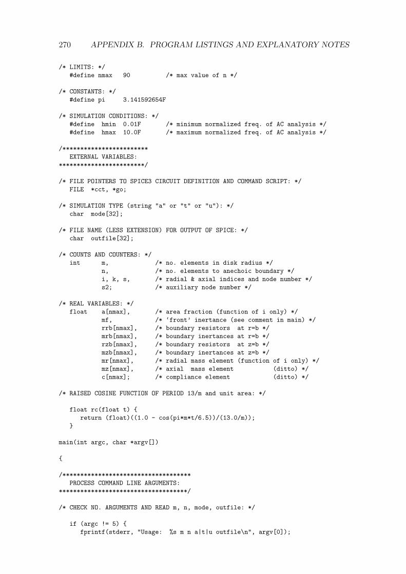
270 APPENDIX B. PROGRAM LISTINGS AND EXPLANATORY NOTES
/* LIMITS: */#define nmax 90 /* max value of n */
/* CONSTANTS: */#define pi 3.141592654F
/* SIMULATION CONDITIONS: */#define hmin 0.01F /* minimum normalized freq. of AC analysis */#define hmax 10.0F /* maximum normalized freq. of AC analysis */
/************************EXTERNAL VARIABLES:
************************/
/* FILE POINTERS TO SPICE3 CIRCUIT DEFINITION AND COMMAND SCRIPT: */FILE *cct, *go;
/* SIMULATION TYPE (string "a" or "t" or "u"): */char mode[32];
/* FILE NAME (LESS EXTENSION) FOR OUTPUT OF SPICE: */char outfile[32];
/* COUNTS AND COUNTERS: */int m, /* no. elements in disk radius */
n, /* no. elements to anechoic boundary */i, k, s, /* radial & axial indices and node number */s2; /* auxiliary node number */
/* REAL VARIABLES: */float a[nmax], /* area fraction (function of i only) */
mf, /* ‘front’ inertance (see comment in main) */rrb[nmax], /* boundary resistors at r=b */mrb[nmax], /* boundary inertances at r=b */rzb[nmax], /* boundary resistors at z=b */mzb[nmax], /* boundary inertances at z=b */mr[nmax], /* radial mass element (function of i only) */mz[nmax], /* axial mass element (ditto) */c[nmax]; /* compliance element (ditto) */
/* RAISED COSINE FUNCTION OF PERIOD 13/m and unit area: */
float rc(float t) return (float)((1.0 - cos(pi*m*t/6.5))/(13.0/m));
main(int argc, char *argv[])
/************************************PROCESS COMMAND LINE ARGUMENTS:
************************************/
/* CHECK NO. ARGUMENTS AND READ m, n, mode, outfile: */
if (argc != 5) fprintf(stderr, "Usage: %s m n a|t|u outfile\n", argv[0]);

B.12. MODEL BUILDER DISK.C (FOR CIRCULAR PISTON) 271
exit(1);if (sscanf(argv[1], "%d", &m) != 1)
fprintf(stderr, "Problem -- possibly non-numeric m.\n");exit(1);
if (sscanf(argv[2], "%d", &n) != 1)
fprintf(stderr, "Problem -- possibly non-numeric n.\n");exit(1);
if (0 >= m || m >= n || n > nmax)
fprintf(stderr, "You must have 0 < m < n <= %d.\n", nmax);exit(1);
strcpy(mode, argv[3]);if (!(*mode == ’a’ || *mode == ’t’ || *mode == ’u’))
fprintf(stderr, "Third argument must be ‘a’ or ‘t’ or ‘u’.\n");exit(1);
strcpy(outfile, argv[4]);
/* IF WE GET THIS FAR, ARGUMENT LIST IS CORRECT! ECHO ARGUMENTS: */
fprintf(stderr,"\n\tm = %d ; n = %d ; mode = %s ; outfile = %s ; nmax = %d.\n",m, n, mode, outfile, nmax);
if (*mode != ’t’)fprintf(stderr, "\tFrequency range: ka = %6.4f to %.1f\n", hmin, hmax);
fprintf(stderr, "\n");
/***********************************EQUIVALENT CIRCUIT COMPONENTS:
***********************************/
/* Area fractions: */for (i=1; i<=m; i++)
a[i] = (2*i - 1.F) / (m*m);/* Front inertance element (parallel combination of axial inertances
adjacent to disk): */mf = 1.F / (2*m);
/* Curved-boundary elements: */for (k=1; k<=n; k++)
rrb[k] = m*m * (float)sqrt(n*n + (k-0.5F)*(k-0.5F)) / (2.F*n*n);mrb[k] = m * (n*n + (k-0.5F)*(k-0.5F)) / (2.F*n*n);
for (i=1; i<=n; i++)
/* Flat-boundary elements: */rzb[i] = 0.5F*m*m * (float)sqrt(1.F/(n*n) + 1/((i-0.5F)*(i-0.5F)));mzb[i] = 0.5F*m * (n/(i-0.5F) + (i-0.5F)/n);
/* Axial inertance elements: */mz[i] = m / (2*i - 1.F);
/* Compliances: */c[i] = (2*i - 1.F) / (m*m*m);
/* Radial inertance elements: */
for (i=1; i<n; i++)mr[i] = m / (2.F * i);
mr[n] = m / (4*n - 1.F); /* truncated at curved boundary */

272 APPENDIX B. PROGRAM LISTINGS AND EXPLANATORY NOTES
/***************************************************WRITE SPICE3 CIRCUIT DEFINITION TO FILE ‘cct’:
***************************************************/
cct = fopen("cct", "w");
/* HEADER: */if (*mode == ’u’)
fprintf(cct, "CIRCULAR RIGID PISTON (UNBAFFLED):\n\n");else
fprintf(cct, "CIRCULAR RIGID PISTON IN INFINITE PLANAR BAFFLE:\n\n");
/* COMMENTS: */fprintf(cct,
"* m = %d ; n = %d ; mode = %s ; outfile = %s ; nmax = %d.\n",m, n, mode, outfile, nmax);
if (*mode != ’t’)fprintf(cct, "* Frequency range: ka = %6.4f to %.1f\n\n", hmin, hmax);
fprintf(cct, "* FDM component values:\n");fprintf(cct, " * m = %d\n", m);fprintf(cct, " * n = %d\n", n);fprintf(cct, " * a[ 1] = %.5f\n", a[1]);fprintf(cct, " * a[%2d] = %.5f\n", m, a[m]);fprintf(cct, " * mf = %.6f\n", mf);fprintf(cct, " * rrb[ 1] = %.5f\n", rrb[1]);fprintf(cct, " * rrb[%2d] = %.5f\n", n, rrb[n]);fprintf(cct, " * mrb[ 1] = %.5f\n", mrb[1]);fprintf(cct, " * mrb[%2d] = %.5f\n", n, mrb[n]);fprintf(cct, " * rzb[ 1] = %.5f\n", rzb[1]);fprintf(cct, " * rzb[%2d] = %.5f\n", n, rzb[n]);fprintf(cct, " * mzb[ 1] = %.5f\n", mzb[1]);fprintf(cct, " * mzb[%2d] = %.5f\n", n, mzb[n]);fprintf(cct, " * mr[ 1] = %.5f\n", mr[1]);fprintf(cct, " * mr[%2d] = %.5f\n", n-1, mr[n-1]);fprintf(cct, " * mr[%2d] = %.5f\n", n, mr[n]);fprintf(cct, " * mz[ 1] = %.5f\n", mz[1]);fprintf(cct, " * mz[%2d] = %.5f\n", n, mz[n]);fprintf(cct, " * c[ 1] = %.7f\n", c[1]);fprintf(cct, " * c[%2d] = %.7f\n", n, c[n]);fprintf(cct, "\n");
/* IF UNBAFFLED, DEFINE AXIAL MASS SUBCIRCUITS ADJACENT TO PLANE OF DISK: */if (*mode == ’u’)
fprintf(cct, "* AXIAL INERTANCE SUBCIRCUITS");fprintf(cct, " ADJACENT TO PLANE OF DISK:\n\n");for (i=m+1; i<=n; i++)
fprintf(cct, ".subckt bplane%02d 1 3\n", i);fprintf(cct, "lzho%02d 1 2 %e\n", i, 0.5F*mz[i]);fprintf(cct, "rzs%02d 2 3 %e\n", i, 1e-6*mz[i]);fprintf(cct, ".ends bplane%02d\n", i);
fprintf(cct, "\n");
/* DEFINE CURVED-BOUNDARY ELEMENT SUBCIRCUITS: */fprintf(cct, "* CURVED-BOUNDARY ELEMENT SUBCIRCUITS:\n\n");if (*mode == ’t’) /* if transient */

B.12. MODEL BUILDER DISK.C (FOR CIRCULAR PISTON) 273
for (k=1; k<=n; k++) fprintf(cct, ".subckt bcurv%02d 1 3\n", k);fprintf(cct, "lr%02d 1 2 %e\n", k, mr[n]);fprintf(cct, "rrb%02d 2 3 %e\n", k, rrb[k]);fprintf(cct, "lrb%02d 2 3 %e\n", k, mrb[k]);fprintf(cct, ".ends bcurv%02d\n", k);
else /* if AC */
for (k=1; k<=n; k++) fprintf(cct, ".subckt bcurv%02d 1 4\n", k);fprintf(cct, "lr%02d 1 2 %e\n", k, mr[n]);fprintf(cct, "rrs%02d 2 3 %e\n", k, 1e-6*mr[n]);fprintf(cct, "rrb%02d 3 4 %e\n", k, rrb[k]);fprintf(cct, "lrb%02d 3 4 %e\n", k, mrb[k]);fprintf(cct, ".ends bcurv%02d\n", k);
fprintf(cct, "\n");
/* DEFINE FLAT-BOUNDARY ELEMENT SUBCIRCUITS: */fprintf(cct, "* FLAT-BOUNDARY ELEMENT SUBCIRCUITS:\n\n");for (i=1; i<=n; i++)
fprintf(cct, ".subckt bflat%02d 1 3\n", i);fprintf(cct, "lzh%02d 1 2 %e\n", i, 0.5F*mz[i]);fprintf(cct, "rzb%02d 2 3 %e\n", i, rzb[i]);fprintf(cct, "lzb%02d 2 3 %e\n", i, mzb[i]);fprintf(cct, ".ends bflat%02d\n", i);
fprintf(cct, "\n");
/* IF AC ANALYSIS REQUIRED, DEFINE RADIAL INERTANCE ELEMENT SUBCIRCUITS: */if (*mode != ’t’)
fprintf(cct, "* RADIAL INERTANCE ELEMENT SUBCIRCUITS:\n\n");for (i=1; i<=n; i++)
fprintf(cct, ".subckt mr%02d 1 3\n", i);fprintf(cct, "lr%02d 1 2 %e\n", i, mr[i]);fprintf(cct, "rrs%02d 2 3 %e\n", i, 1e-6*mr[i]);fprintf(cct, ".ends mr%02d\n", i);
fprintf(cct, "\n");
/* SOURCE: */fprintf(cct, "* SOURCE:\n\n");if (*mode == ’t’)
fprintf(cct, "Vtran %2d 0 dc 0 pwl ( 0 0\n", m+1);for (i=1; i<=25; i++)
fprintf(cct, "+ %.6f %.7f\n", (float)i/(2*m), rc((double)i/(2*m)));fprintf(cct, "+ %.6f 0 )\n", 13.F/m);
elsefprintf(cct, "Iac 0 %2d dc 0 ac 1\n", m+1);
fprintf(cct, "\n");
/* SPLIT FLUX AND AVERAGE BACK PRESSURES: */fprintf(cct, "* SPLIT FLUX AND AVERAGE BACK PRESSURES:\n\n");for (i=1; i<=m; i++)
fprintf(cct, "F%02d 0 %2d E01 %e\n", i, m+1+i, a[i]);for (i=1; i<=m; i++)
fprintf(cct, "E%02d %2d %2d %2d 0 %e\n", i, i+1, i, m+1+i, a[i]);

274 APPENDIX B. PROGRAM LISTINGS AND EXPLANATORY NOTES
fprintf(cct, "\n");
/* WRITE FRONT INERTANCE: */fprintf(cct, "* FRONT INERTANCE:\n\n");fprintf(cct, "lf 1 0 %e\n", mf);fprintf(cct, "\n");
/* IF DISK IS UNBAFFLED, WRITE AXIAL MASSES ADJACENT TO PLANE OF DISK: */if (*mode == ’u’)
fprintf(cct, "* AXIAL INERTANCE ELEMENTS");fprintf(cct, " ADJACENT TO PLANE OF DISK:\n\n");for (i=m+1; i<=n; i++)
s = m + 1 + i;fprintf(cct, "xbplane%02d %2d 0 bplane%02d\n", i, s, i);
fprintf(cct, "\n");
/* WRITE CURVED-BOUNDARY ELEMENTS: */fprintf(cct, "* CURVED-BOUNDARY ELEMENTS:\n\n");for (k=1; k<=n; k++)
s = m + 1 + k*n;fprintf(cct, "xbcurv%02d %4d 0 bcurv%02d\n", k, s, k);
fprintf(cct, "\n");
/* WRITE FLAT-BOUNDARY ELEMENTS: */fprintf(cct, "* FLAT-BOUNDARY ELEMENTS:\n\n");for (i=1; i<=n; i++)
s = m + 1 + (n-1)*n + i;fprintf(cct, "xbflat%02d %4d 0 bflat%02d\n", i, s, i);
fprintf(cct, "\n");
/* WRITE RADIAL INERTANCE ELEMENTS: */fprintf(cct, "* RADIAL INERTANCE ELEMENTS:\n\n");for (k=1; k<=n; k++)
for (i=1; i<n; i++) /* only n-1 elements in radial direction */ s = m + 1 + (k-1)*n + i;if (*mode == ’t’)
fprintf(cct, "lr%02d%02d %4d %4d %e\n", i, k, s, s+1, mr[i]);else
fprintf(cct, "xmr%02d%02d %4d %4d mr%02d\n", i, k, s, s+1, i);
fprintf(cct, "\n");
/* WRITE AXIAL INERTANCE ELEMENTS: */fprintf(cct, "* AXIAL INERTANCE ELEMENTS:\n\n");for (k=1; k<n; k++) /* only n-1 elements in axial direction */
for (i=1; i<=n; i++) s = m + 1 + (k-1)*n + i;fprintf(cct, "lz%02d%02d %4d %4d %e\n", i, k, s, s+n, mz[i]);
fprintf(cct, "\n");
/* WRITE COMPLIANCE ELEMENTS: */fprintf(cct, "* COMPLIANCE ELEMENTS:\n\n");for (k=1; k<=n; k++)
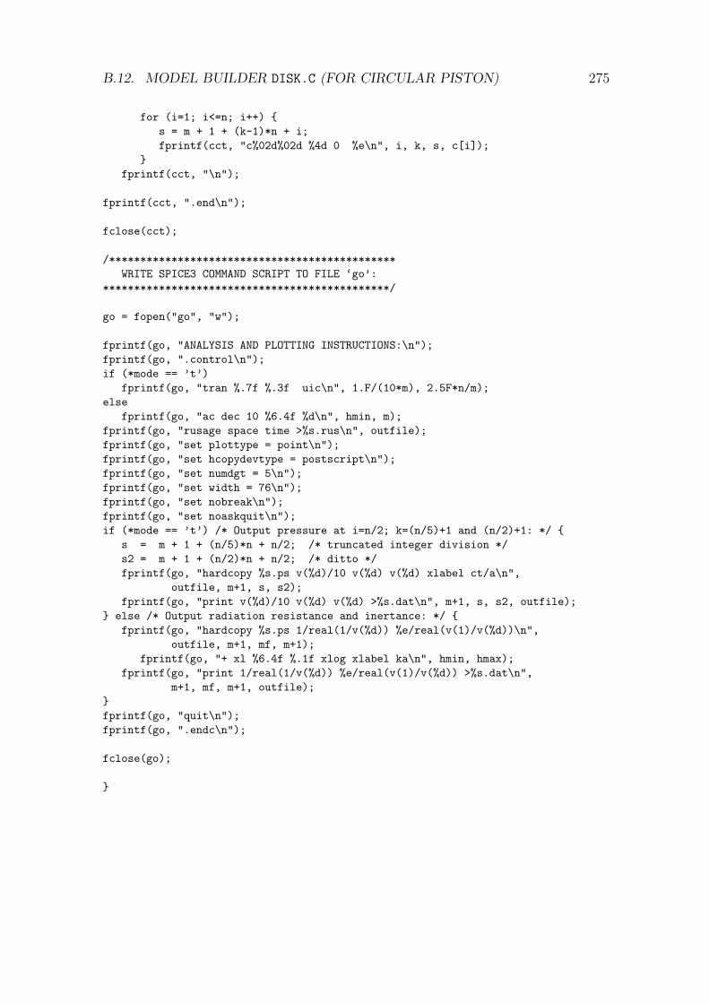
B.12. MODEL BUILDER DISK.C (FOR CIRCULAR PISTON) 275
for (i=1; i<=n; i++) s = m + 1 + (k-1)*n + i;fprintf(cct, "c%02d%02d %4d 0 %e\n", i, k, s, c[i]);
fprintf(cct, "\n");
fprintf(cct, ".end\n");
fclose(cct);
/**********************************************WRITE SPICE3 COMMAND SCRIPT TO FILE ‘go’:
**********************************************/
go = fopen("go", "w");
fprintf(go, "ANALYSIS AND PLOTTING INSTRUCTIONS:\n");fprintf(go, ".control\n");if (*mode == ’t’)
fprintf(go, "tran %.7f %.3f uic\n", 1.F/(10*m), 2.5F*n/m);else
fprintf(go, "ac dec 10 %6.4f %d\n", hmin, m);fprintf(go, "rusage space time >%s.rus\n", outfile);fprintf(go, "set plottype = point\n");fprintf(go, "set hcopydevtype = postscript\n");fprintf(go, "set numdgt = 5\n");fprintf(go, "set width = 76\n");fprintf(go, "set nobreak\n");fprintf(go, "set noaskquit\n");if (*mode == ’t’) /* Output pressure at i=n/2; k=(n/5)+1 and (n/2)+1: */
s = m + 1 + (n/5)*n + n/2; /* truncated integer division */s2 = m + 1 + (n/2)*n + n/2; /* ditto */fprintf(go, "hardcopy %s.ps v(%d)/10 v(%d) v(%d) xlabel ct/a\n",
outfile, m+1, s, s2);fprintf(go, "print v(%d)/10 v(%d) v(%d) >%s.dat\n", m+1, s, s2, outfile);
else /* Output radiation resistance and inertance: */ fprintf(go, "hardcopy %s.ps 1/real(1/v(%d)) %e/real(v(1)/v(%d))\n",
outfile, m+1, mf, m+1);fprintf(go, "+ xl %6.4f %.1f xlog xlabel ka\n", hmin, hmax);
fprintf(go, "print 1/real(1/v(%d)) %e/real(v(1)/v(%d)) >%s.dat\n",m+1, mf, m+1, outfile);
fprintf(go, "quit\n");fprintf(go, ".endc\n");
fclose(go);

276 APPENDIX B. PROGRAM LISTINGS AND EXPLANATORY NOTES
B.13 Sample circuit file d35u.cir (for circular pis-ton)
The circuit files produced by the program disk.c were initially called “cct”, butwere manually renamed for permanent storage. The name d35u.cir is mnemonic,indicating that the file was produced by disk.c with m = 3 and n = 5 for theunbaffled case. The unbaffled version is chosen for illustration because it yields a“fully-optioned” equivalent circuit—all truncated axial mass elements are included,and subcircuits must be defined in order to remove zero-resistance loops.
The letter “b” in a subcircuit name stands for “boundary”. While the definitionof a subcircuit can be named arbitrarily, SPICE requires each instance of a subcir-cuit to have a name beginning with “x” or “X”. Mass elements must have namesbeginning with “l” or “L” in SPICE, although the text of this thesis prefers “m”or “M”. The names of components include row and/or column numbers to ensureuniqueness.
The circuit file is listed below.
CIRCULAR RIGID PISTON (UNBAFFLED):
* m = 3 ; n = 5 ; mode = u ; outfile = d35u ; nmax = 90.* Frequency range: ka = 0.0100 to 10.0
* FDM component values:* m = 3* n = 5* a[ 1] = 0.11111* a[ 3] = 0.55556* mf = 0.166667* rrb[ 1] = 0.90449* rrb[ 5] = 1.21083* mrb[ 1] = 1.51500* mrb[ 5] = 2.71500* rzb[ 1] = 9.04489* rzb[ 5] = 1.34536* mzb[ 1] = 15.15000* mzb[ 5] = 3.01667* mr[ 1] = 1.50000* mr[ 4] = 0.37500* mr[ 5] = 0.15789* mz[ 1] = 3.00000* mz[ 5] = 0.33333* c[ 1] = 0.0370370* c[ 5] = 0.3333333
* AXIAL INERTANCE SUBCIRCUITS ADJACENT TO PLANE OF DISK:
.subckt bplane04 1 3lzho04 1 2 2.142857e-01rzs04 2 3 4.285714e-07.ends bplane04.subckt bplane05 1 3lzho05 1 2 1.666667e-01rzs05 2 3 3.333333e-07.ends bplane05

B.13. SAMPLE CIRCUIT FILE D35U.CIR (FOR CIRCULAR PISTON) 277
* CURVED-BOUNDARY ELEMENT SUBCIRCUITS:
.subckt bcurv01 1 4lr01 1 2 1.578947e-01rrs01 2 3 1.578947e-07rrb01 3 4 9.044887e-01lrb01 3 4 1.515000e+00.ends bcurv01.subckt bcurv02 1 4lr02 1 2 1.578947e-01rrs02 2 3 1.578947e-07rrb02 3 4 9.396276e-01lrb02 3 4 1.635000e+00.ends bcurv02.subckt bcurv03 1 4lr03 1 2 1.578947e-01rrs03 2 3 1.578947e-07rrb03 3 4 1.006231e+00lrb03 3 4 1.875000e+00.ends bcurv03.subckt bcurv04 1 4lr04 1 2 1.578947e-01rrs04 2 3 1.578947e-07rrb04 3 4 1.098590e+00lrb04 3 4 2.235000e+00.ends bcurv04.subckt bcurv05 1 4lr05 1 2 1.578947e-01rrs05 2 3 1.578947e-07rrb05 3 4 1.210826e+00lrb05 3 4 2.715000e+00.ends bcurv05
* FLAT-BOUNDARY ELEMENT SUBCIRCUITS:
.subckt bflat01 1 3lzh01 1 2 1.500000e+00rzb01 2 3 9.044888e+00lzb01 2 3 1.515000e+01.ends bflat01.subckt bflat02 1 3lzh02 1 2 5.000000e-01rzb02 2 3 3.132092e+00lzb02 2 3 5.450000e+00.ends bflat02.subckt bflat03 1 3lzh03 1 2 3.000000e-01rzb03 2 3 2.012461e+00lzb03 2 3 3.750000e+00.ends bflat03.subckt bflat04 1 3lzh04 1 2 2.142857e-01rzb04 2 3 1.569414e+00lzb04 2 3 3.192857e+00.ends bflat04.subckt bflat05 1 3lzh05 1 2 1.666667e-01

278 APPENDIX B. PROGRAM LISTINGS AND EXPLANATORY NOTES
rzb05 2 3 1.345362e+00lzb05 2 3 3.016667e+00.ends bflat05
* RADIAL INERTANCE ELEMENT SUBCIRCUITS:
.subckt mr01 1 3lr01 1 2 1.500000e+00rrs01 2 3 1.500000e-06.ends mr01.subckt mr02 1 3lr02 1 2 7.500000e-01rrs02 2 3 7.500000e-07.ends mr02.subckt mr03 1 3lr03 1 2 5.000000e-01rrs03 2 3 5.000000e-07.ends mr03.subckt mr04 1 3lr04 1 2 3.750000e-01rrs04 2 3 3.750000e-07.ends mr04.subckt mr05 1 3lr05 1 2 1.578947e-01rrs05 2 3 1.578947e-07.ends mr05
* SOURCE:
Iac 0 4 dc 0 ac 1
* SPLIT FLUX AND AVERAGE BACK PRESSURES:
F01 0 5 E01 1.111111e-01F02 0 6 E01 3.333333e-01F03 0 7 E01 5.555556e-01E01 2 1 5 0 1.111111e-01E02 3 2 6 0 3.333333e-01E03 4 3 7 0 5.555556e-01
* FRONT INERTANCE:
lf 1 0 1.666667e-01
* AXIAL INERTANCE ELEMENTS ADJACENT TO PLANE OF DISK:
xbplane04 8 0 bplane04xbplane05 9 0 bplane05
* CURVED-BOUNDARY ELEMENTS:
xbcurv01 9 0 bcurv01xbcurv02 14 0 bcurv02xbcurv03 19 0 bcurv03xbcurv04 24 0 bcurv04xbcurv05 29 0 bcurv05
* FLAT-BOUNDARY ELEMENTS:

B.13. SAMPLE CIRCUIT FILE D35U.CIR (FOR CIRCULAR PISTON) 279
xbflat01 25 0 bflat01xbflat02 26 0 bflat02xbflat03 27 0 bflat03xbflat04 28 0 bflat04xbflat05 29 0 bflat05
* RADIAL INERTANCE ELEMENTS:
xmr0101 5 6 mr01xmr0201 6 7 mr02xmr0301 7 8 mr03xmr0401 8 9 mr04xmr0102 10 11 mr01xmr0202 11 12 mr02xmr0302 12 13 mr03xmr0402 13 14 mr04xmr0103 15 16 mr01xmr0203 16 17 mr02xmr0303 17 18 mr03xmr0403 18 19 mr04xmr0104 20 21 mr01xmr0204 21 22 mr02xmr0304 22 23 mr03xmr0404 23 24 mr04xmr0105 25 26 mr01xmr0205 26 27 mr02xmr0305 27 28 mr03xmr0405 28 29 mr04
* AXIAL INERTANCE ELEMENTS:
lz0101 5 10 3.000000e+00lz0201 6 11 1.000000e+00lz0301 7 12 6.000000e-01lz0401 8 13 4.285714e-01lz0501 9 14 3.333333e-01lz0102 10 15 3.000000e+00lz0202 11 16 1.000000e+00lz0302 12 17 6.000000e-01lz0402 13 18 4.285714e-01lz0502 14 19 3.333333e-01lz0103 15 20 3.000000e+00lz0203 16 21 1.000000e+00lz0303 17 22 6.000000e-01lz0403 18 23 4.285714e-01lz0503 19 24 3.333333e-01lz0104 20 25 3.000000e+00lz0204 21 26 1.000000e+00lz0304 22 27 6.000000e-01lz0404 23 28 4.285714e-01lz0504 24 29 3.333333e-01
* COMPLIANCE ELEMENTS:
c0101 5 0 3.703704e-02c0201 6 0 1.111111e-01c0301 7 0 1.851852e-01

280 APPENDIX B. PROGRAM LISTINGS AND EXPLANATORY NOTES
c0401 8 0 2.592593e-01c0501 9 0 3.333333e-01c0102 10 0 3.703704e-02c0202 11 0 1.111111e-01c0302 12 0 1.851852e-01c0402 13 0 2.592593e-01c0502 14 0 3.333333e-01c0103 15 0 3.703704e-02c0203 16 0 1.111111e-01c0303 17 0 1.851852e-01c0403 18 0 2.592593e-01c0503 19 0 3.333333e-01c0104 20 0 3.703704e-02c0204 21 0 1.111111e-01c0304 22 0 1.851852e-01c0404 23 0 2.592593e-01c0504 24 0 3.333333e-01c0105 25 0 3.703704e-02c0205 26 0 1.111111e-01c0305 27 0 1.851852e-01c0405 28 0 2.592593e-01c0505 29 0 3.333333e-01
.end

B.14. TABLE-FORMATTING PROGRAMS 281
B.14 Table-formatting programs
Programs taba.c and tabu.c produced Tables 11.1 and 11.2, respectively. Theprograms are quite trivial and are listed only for the sake of completeness. Mostof the code (73 lines out of 83, including comments) is common to both. Eachprogram combines five SPICE output files (produced by the “print” command)into a single formatted file. The mnemonic names of the SPICE files appear in theopening comments; each SPICE file corresponds to one pair of values of m and nand is named accordingly.
After inspecting the results of the first successful run, the author decided thatsufficient data would be obtained by taking every second line of the SPICE files,i.e. every second frequency in the AC analyses. This decision is seen in the function“extract”, which appears in both programs.
The listings follow.
/****************************************************************************
PROGRAM ‘taba.c’ (GAVIN R. PUTLAND)
Collect files d618a.dat, d721a.dat, d824a.dat, d621a.dat and d828a.datinto a single presentable plain-text table, written to standard output.
****************************************************************************/
#include <stdio.h>#include <math.h>#include <string.h>
#define pi 3.141592654F
/* GLOBAL VARIABLES: */
FILE *file;
char line[99], filename[32];
int i;
float f[13], /* frequency */r6[13], r7[13], r8[13], r62[13], r82[13], /* rad. resistance */m6[13], m7[13], m8[13], m62[13], m82[13]; /* rad. inertance */
/* FUNCTION TO EXTRACT DATA FROM ONE FILE: */
void extract(char *filename, float *r, float *m)
file = fopen(filename, "r");/* SKIP FIRST FIVE LINES (PREAMBLE): */
for (i=0; i<5; i++)fgets(line, 99, file);
/* READ ALTERNATE LINES; EXTRACT r, m: */for (i=0; i<13; i++)
fgets(line, 99, file);sscanf(line, "%*d %*e, %*e %e %e", r+i, m+i);fgets(line, 99, file);

282 APPENDIX B. PROGRAM LISTINGS AND EXPLANATORY NOTES
fclose(file);
main()
/* HEAD TABLE: */
printf("\n");printf(" m,n: %7s %7s %7s %7s %7s\n\n",
"6,18 ", "7,21 ", "8,24 ", "6,21 ", "8,28 ");
/* GET NUMBERS: */
for (i=0; i<13; i++)f[i] = 0.01 * pow(10.0, 0.2*i);
extract("d618a.dat", r6, m6);extract("d721a.dat", r7, m7);extract("d824a.dat", r8, m8);extract("d621a.dat", r62, m62);extract("d828a.dat", r82, m82);
/* PRINT RADIATION RESISTANCE: */
printf(" f h Resistance (LF limit = 1.4410):\n\n");for (i=0; i<13; i++)
printf("%6.4f %7.4f %7.4f %7.4f %7.4f %7.4f %7.4f\n",f[i], 2*pi*f[i], r6[i], r7[i], r8[i], r62[i], r82[i]);
printf("\n");
/* PRINT RADIATION INERTANCE: */
printf(" f h Inertance (LF limit = 0.8488):\n\n");for (i=0; i<13; i++)
printf("%6.4f %7.4f %7.4f %7.4f %7.4f %7.4f %7.4f\n",f[i], 2*pi*f[i], m6[i], m7[i], m8[i], m62[i], m82[i]);
printf("\n");
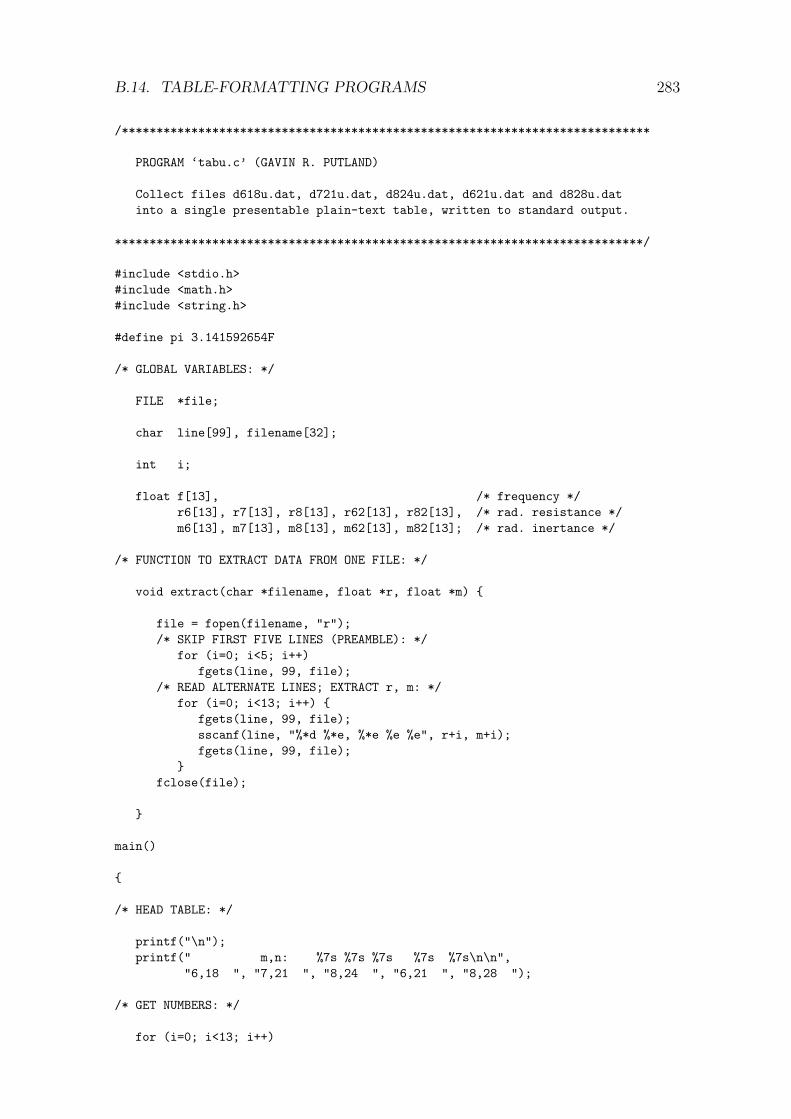
B.14. TABLE-FORMATTING PROGRAMS 283
/****************************************************************************
PROGRAM ‘tabu.c’ (GAVIN R. PUTLAND)
Collect files d618u.dat, d721u.dat, d824u.dat, d621u.dat and d828u.datinto a single presentable plain-text table, written to standard output.
****************************************************************************/
#include <stdio.h>#include <math.h>#include <string.h>
#define pi 3.141592654F
/* GLOBAL VARIABLES: */
FILE *file;
char line[99], filename[32];
int i;
float f[13], /* frequency */r6[13], r7[13], r8[13], r62[13], r82[13], /* rad. resistance */m6[13], m7[13], m8[13], m62[13], m82[13]; /* rad. inertance */
/* FUNCTION TO EXTRACT DATA FROM ONE FILE: */
void extract(char *filename, float *r, float *m)
file = fopen(filename, "r");/* SKIP FIRST FIVE LINES (PREAMBLE): */
for (i=0; i<5; i++)fgets(line, 99, file);
/* READ ALTERNATE LINES; EXTRACT r, m: */for (i=0; i<13; i++)
fgets(line, 99, file);sscanf(line, "%*d %*e, %*e %e %e", r+i, m+i);fgets(line, 99, file);
fclose(file);
main()
/* HEAD TABLE: */
printf("\n");printf(" m,n: %7s %7s %7s %7s %7s\n\n",
"6,18 ", "7,21 ", "8,24 ", "6,21 ", "8,28 ");
/* GET NUMBERS: */
for (i=0; i<13; i++)

284 APPENDIX B. PROGRAM LISTINGS AND EXPLANATORY NOTES
f[i] = 0.01 * pow(10.0, 0.2*i);
extract("d618u.dat", r6, m6);extract("d721u.dat", r7, m7);extract("d824u.dat", r8, m8);extract("d621u.dat", r62, m62);extract("d828u.dat", r82, m82);
/* PRINT RADIATION RESISTANCE: */
printf(" f h Resistance:\n\n");for (i=0; i<13; i++)
printf("%6.4f %7.4f %7.4f %7.4f %7.4f %7.4f %7.4f\n",f[i], 2*pi*f[i], r6[i], r7[i], r8[i], r62[i], r82[i]);
printf("\n");
/* PRINT RADIATION INERTANCE: */
printf(" f h Inertance (LF limit approx. 0.425):\n\n");for (i=0; i<13; i++)
printf("%6.4f %7.4f %7.3f %7.3f %7.3f %7.3f %7.3f\n",f[i], 2*pi*f[i], m6[i], m7[i], m8[i], m62[i], m82[i]);
printf("\n");

B.15. TRANSIENT RESPONSE PLOTTER TR2TEX.C 285
B.15 Transient response plotter tr2tex.c
The procedure for drawing Fig. 11.2 was as follows. First, program disk.c was runwith m = 4, n = 32 and mode= "t", to produce a circuit definition file and commandscript for SPICE. Running SPICE then produced a text file whose columns indicatedthe transient responses at the three points of interest. Finally, program tr2tex.cwas run, converting the SPICE output file to a set of LATEX picture commands.
Program tr2tex.c is listed below. It makes no pretensions of generality. Onlythe last part of the program processes the SPICE file and plots the points. Therest of it is concerned with the picture objects that form the axes, labels, insets,reflection marks, etc.; the coordinates of these objects were all calculated manually.
/****************************************************************************
PROGRAM ‘tr2tex.c’ (GAVIN R. PUTLAND)Convert a triple transient response in SPICE3 ‘print col’ formatto a graph using LaTeX ‘picture’ commands.
USAGE (assuming executable file is called ‘tr2tex’):
tr2tex in out
where ‘in’ is the name of the SPICE file and ‘out’ is the name of theoutput file. If out exists, tr2tex absolutely refuses to overwrite it.The out file begins with
\setlength\unitlength0.0033333in\beginpicture(1600,2300)(-60,-250)
and ends with
\endpicture
The present version draws axes and grids assuming that the time columnextends extends from 0 to 20 units and that the ordinates are in theranges 0 to 65, -5 to 85, and -10 to 70. The first ordinate is assumedto be tabulated at one tenth of the scale of the other two, and isgraphed at one twentieth.
****************************************************************************/
#include <stdio.h>#include <math.h>#include <string.h>
main(int argc, char *argv[])
/* FILE NAMES AND POINTERS: */
char inname[32], outname[32];FILE *in, *out;
/* SCRATCH VARIABLES */
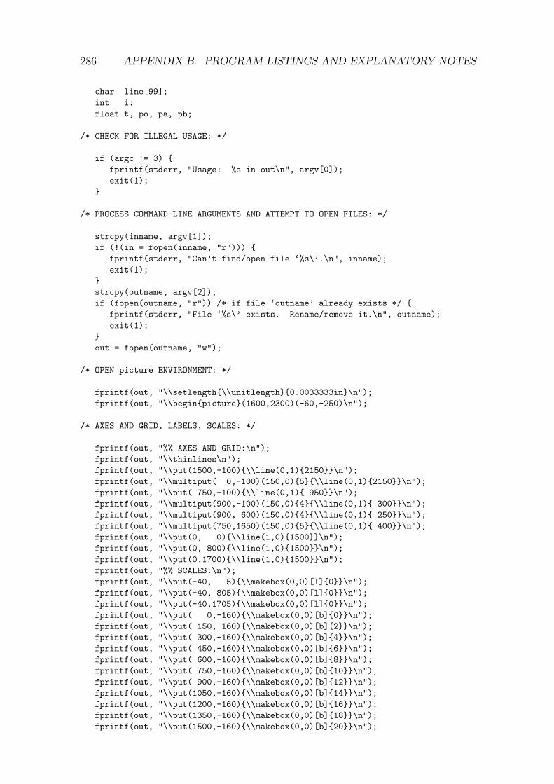
286 APPENDIX B. PROGRAM LISTINGS AND EXPLANATORY NOTES
char line[99];int i;float t, po, pa, pb;
/* CHECK FOR ILLEGAL USAGE: */
if (argc != 3) fprintf(stderr, "Usage: %s in out\n", argv[0]);exit(1);
/* PROCESS COMMAND-LINE ARGUMENTS AND ATTEMPT TO OPEN FILES: */
strcpy(inname, argv[1]);if (!(in = fopen(inname, "r")))
fprintf(stderr, "Can’t find/open file ‘%s\’.\n", inname);exit(1);
strcpy(outname, argv[2]);if (fopen(outname, "r")) /* if file ‘outname’ already exists */
fprintf(stderr, "File ‘%s\’ exists. Rename/remove it.\n", outname);exit(1);
out = fopen(outname, "w");
/* OPEN picture ENVIRONMENT: */
fprintf(out, "\\setlength\\unitlength0.0033333in\n");fprintf(out, "\\beginpicture(1600,2300)(-60,-250)\n");
/* AXES AND GRID, LABELS, SCALES: */
fprintf(out, "%% AXES AND GRID:\n");fprintf(out, "\\thinlines\n");fprintf(out, "\\put(1500,-100)\\line(0,1)2150\n");fprintf(out, "\\multiput( 0,-100)(150,0)5\\line(0,1)2150\n");fprintf(out, "\\put( 750,-100)\\line(0,1) 950\n");fprintf(out, "\\multiput(900,-100)(150,0)4\\line(0,1) 300\n");fprintf(out, "\\multiput(900, 600)(150,0)4\\line(0,1) 250\n");fprintf(out, "\\multiput(750,1650)(150,0)5\\line(0,1) 400\n");fprintf(out, "\\put(0, 0)\\line(1,0)1500\n");fprintf(out, "\\put(0, 800)\\line(1,0)1500\n");fprintf(out, "\\put(0,1700)\\line(1,0)1500\n");fprintf(out, "%% SCALES:\n");fprintf(out, "\\put(-40, 5)\\makebox(0,0)[l]0\n");fprintf(out, "\\put(-40, 805)\\makebox(0,0)[l]0\n");fprintf(out, "\\put(-40,1705)\\makebox(0,0)[l]0\n");fprintf(out, "\\put( 0,-160)\\makebox(0,0)[b]0\n");fprintf(out, "\\put( 150,-160)\\makebox(0,0)[b]2\n");fprintf(out, "\\put( 300,-160)\\makebox(0,0)[b]4\n");fprintf(out, "\\put( 450,-160)\\makebox(0,0)[b]6\n");fprintf(out, "\\put( 600,-160)\\makebox(0,0)[b]8\n");fprintf(out, "\\put( 750,-160)\\makebox(0,0)[b]10\n");fprintf(out, "\\put( 900,-160)\\makebox(0,0)[b]12\n");fprintf(out, "\\put(1050,-160)\\makebox(0,0)[b]14\n");fprintf(out, "\\put(1200,-160)\\makebox(0,0)[b]16\n");fprintf(out, "\\put(1350,-160)\\makebox(0,0)[b]18\n");fprintf(out, "\\put(1500,-160)\\makebox(0,0)[b]20\n");

B.15. TRANSIENT RESPONSE PLOTTER TR2TEX.C 287
fprintf(out, "%% LABELS:\n");fprintf(out, "\\put(750,-230)\\makebox(0,0)[b]Normalized time");
fprintf(out, " $\\,\\hatt=ct/a$\n");fprintf(out, "\\small\n");fprintf(out, "\\put(177,1950)Mean pressure over source");
fprintf(out, " $\\times\\,\\frac120$\n");fprintf(out, "\\put( 63,1550)Pressure at $A$\n");fprintf(out, "\\put(170, 600)Pressure at $B$\n");fprintf(out, "%% REFLECTION MARKS AND LABELS:\n");fprintf(out, "\\thicklines\n");fprintf(out, "\\put( 437,840)\\line(0,1)60\n");fprintf(out, "\\put( 546, 40)\\line(0,1)60\n");fprintf(out, "\\put(1039,700)\\line(0,1)60\n");fprintf(out, "\\put(1238,700)\\line(0,1)60\n");fprintf(out, "\\put(1475,700)\\line(0,1)60\n");fprintf(out, "\\put(1082, 40)\\line(0,1)60\n");fprintf(out, "\\put(1059, 40)\\line(0,1)60\n");fprintf(out, "\\put(1395, 40)\\line(0,1)60\n");fprintf(out, "\\put(1025,660)$r$\n");fprintf(out, "\\put(1228,660)$z$\n");fprintf(out, "\\put(1415,660)$z,B$\n");fprintf(out, "\\put(1080,110)$r$\n");fprintf(out, "\\put(1055,110)$z$\n");fprintf(out, "\\put(1362,110)$r,z$\n");fprintf(out, "%% DRAW LOWER INSET:\n");fprintf(out, "\\put( 810, 520)Residual reflections (peak)\n");fprintf(out, "\\put( 810, 470)predicted by geometrical optics:\n");fprintf(out, "\\put( 870, 410)$\\,r\\;$: from boundary $r=b$\\,;\n");fprintf(out, "\\put( 870, 360)$\\,z\\;$: from boundary $z=b$\\,;\n");fprintf(out, "\\put( 870, 310)$B$\\,: from baffle.\n");fprintf(out, "\\put( 810, 250)Unlabeled bars show direct wave.\n");fprintf(out, "%% DRAW UPPER INSET:\n");fprintf(out, "\\put( 790, 950)\\vector(1,0)550\n");fprintf(out, "\\put( 790, 950)\\vector(0,1)550\n");fprintf(out, "\\put( 790, 953)\\line(1,0)60\n");fprintf(out, "\\put( 790, 947)\\line(1,0)60\n");fprintf(out, "\\thinlines\n");fprintf(out, "\\put( 790,1430)\\line(1,0)480\n");fprintf(out, "\\put(1270, 950)\\line(0,1) 65\n");fprintf(out, "\\put(1270,1080)\\line(0,1) 85\n");fprintf(out, "\\put(1270,1230)\\line(0,1)200\n");fprintf(out, "\\put( 790, 900)\\makebox(0,0)[b]0\n");fprintf(out, "\\put( 850, 900)\\makebox(0,0)[b]$a$\n");fprintf(out, "\\put(1270, 900)\\makebox(0,0)[b]$b$\n");fprintf(out, "\\put( 770, 955)\\makebox(0,0)[r]0\n");fprintf(out, "\\put( 770,1435)\\makebox(0,0)[r]$b$\n");fprintf(out, "\\put(1370, 961)\\makebox(0,0)[t]$r$\n");fprintf(out, "\\put( 790,1536)\\makebox(0,0)[t]$z$\n");fprintf(out, "\\put(1022,1047)\\circle*12\n");fprintf(out, "\\put(1022,1197)\\circle*12\n");fprintf(out,
"\\put(1040,1035)$A\\,(15.5\\,\\Delta r,6.5\\,\\Delta z)$\n");fprintf(out,
"\\put(1040,1185)$B\\,(15.5\\,\\Delta r,16.5\\,\\Delta z)$\n");fprintf(out, "\\put( 802, 968)\\footnotesize\\sl Source\n");fprintf(out, "\\put(1070, 905)\\sl Baffle\n");fprintf(out, "\\put( 845,1385)\\sl Anechoic boundaries\n");fprintf(out, "\\put( 690,1235)\\sl Axis\n");

288 APPENDIX B. PROGRAM LISTINGS AND EXPLANATORY NOTES
fprintf(out, "\\put( 910,1560)$a=4\\,\\Delta r=\\:$source radius\n");fprintf(out, "\\put( 910,1500)$b=32\\,\\Delta r=32\\,\\Delta z$\n");
/* PROCESS SPICE FILE: */
fprintf(out, "%% POINTS FROM FILE ‘%s\’:\n", inname);/* SKIP FIRST FIVE LINES (PREAMBLE): */
for (i=0; i<5; i++)fgets(line, 99, in);
/* READ LINES; EXTRACT COORDINATES, PLOT POINTS: */while (fgets(line, 99, in))
sscanf(line, "%*d %e %e %e %e", &t, &po, &pa, &pb);t = 75.F * t;po = 5000.F * po + 1700.F;
pa = 10000.F * pa + 800.F;pb = 10000.F * pb;fprintf(out, "\\put(%5.0f,%5.0f)\\circle*8\n", t, po);
fprintf(out, "\\put(%5.0f,%5.0f)\\circle*8\t", t, pa);fprintf(out, "\\put(%5.0f,%5.0f)\\circle*8\n", t, pb);
/* CLOSE picture ENVIRONMENT AND CLOSE FILES: */
fprintf(out, "\\endpicture\n");fclose(in);fclose(out);

Bibliography
[1] Altronics Electronic Components Catalogue, 12th Ed. (Perth, 1993), pp. 34–5,cat. nos. C 3065, C 3034.
[2] M.Arai: “Study on Acoustic Filters by an Electric Simulator”, J. AcousticalSoc. of Japan, vol. 16 (1960), pp. 16–28. In Japanese, with English abstract.
[3] G. L. Augspurger: “Theory, ingenuity, and wishful wizardry in loudspeakerdesign—A half-century of progress?”, J. Acoustical Soc. of America, vol. 77,pp. 1303–8 (1985 April). Comments by E. Villchur: vol. 79, pp. 177–9 (1986 Jan-uary).
[4] S. Ballantine: “On the Propagation of Sound in the General Bessel Horn of Infi-nite Length”, J. Franklin Inst., vol. 203, pp. 85–102 (1927 January). Commentsby C.R.Hanna, and reply: vol. 203, pp. 849–53 (1927 June).
[5] D.A. Barlow: “Rigidity of Loudspeaker Diaphragms”, Wireless World, vol. 64,pp. 564–9 (1958 December).
[6] D.A. Barlow: “The Development of a Sandwich-Construction Loudspeaker Sys-tem”, J. Audio Engineering Soc., vol. 18, pp. 269–81 (1970 June). Reprintedin Loudspeakers: An Anthology, 2nd Ed. (New York, Audio Eng. Soc., 1980),pp. 159–71.
[7] D.A.Barlow: “Loudspeaker Coloration”, Wireless World, vol. 84, no. 1507,pp. 34–7 (1978 March).
[8] D.A. Barlow, G. D.Galletly & J.Mistry: “The Resonances of Loudspeaker Di-aphragms”, J. Audio Engineering Soc., vol. 29, pp. 699–704 (1981 October).Reprinted in Loudspeakers Vol. 2: An Anthology (New York, Audio Eng. Soc.,1984), pp. 251–6.
[9] G.M. Barrow: Physical Chemistry, 4th ed. (New York: McGraw-Hill, 1979).
[10] A. H.Benade & E. V. Jansson: “On Plane and Spherical Waves in Horns withNonuniform Flare: I. Theory of Radiation, Resonance Frequencies, and ModeConversion”, Acustica, vol. 31, no. 2, pp. 79–98 (1974 August).
[11] L. L. Beranek: Acoustics (New York: McGraw-Hill, 1954).
[12] L. Bianchi: Lezioni di geometria differenziale (Pisa: Spoerri, 1894). In Italian.Third edition: vol. 1, 1922; vol. 2, 1923. German translation by M.Lukat: Vor-lesungen uber Differentialgeometrie, 2e Aufl. (Leipzig: Teubner, 1910). Citedby Struik [55].
289

290 BIBLIOGRAPHY
[13] L. J. S. Bradbury: “The Use of Fibrous Materials in Loudspeaker Enclosures”,J. Audio Engineering Soc., vol. 24, pp. 162–70 (1976 April). Reprinted in Loud-speakers: An Anthology, 2nd Ed. (New York, Audio Eng. Soc., 1980), pp. 404–12.
[14] L.M.Chase: “The Thermo-Acoustic Properties of Fibrous Material”, IEEETrans. on Acoustics, Speech, and Signal Processing, vol. ASSP-22, pp. 297–300(1974 August).
[15] G.Darboux: Lecons sur la theorie generale des surfaces (Paris: Gauthier-Villars). In French. First edition: vol. 1, 1887; vol. 2, 1889; vol. 3, 1894; vol. 4,1896. Second edition: four volumes, 1914. Cited by Struik [55].
[16] E. Eisner: “Complete Solutions of the ‘Webster’ Horn Equation”, J. AcousticalSoc. of America, vol. 41, pp. 1126–46 (1967 April).
[17] J. E. Freehafer: “The Acoustical Impedance of an Infinite Hyperbolic Horn”, J.Acoustical Soc. of America, vol. 11, pp. 467–476 (1940 April).
[18] E.R.Geddes: “Acoustic Waveguide Theory”, J. Audio Engineering Soc.,vol. 37, pp. 554–69 (1989 July/Aug.).
[19] E.R. Geddes: “Acoustic Waveguide Theory Revisited”, J. Audio EngineeringSoc., vol. 41, pp. 452–61 (1993 June).
[20] E.R.Geddes: “Sound Radiation from Acoustic Apertures”, J. Audio Engineer-ing Soc., vol. 41, pp. 214–30 (1993 April).
[21] D. E.Gray (ed.): American Institute of Physics Handbook, 3rd ed. (New York:McGraw-Hill, 1972).
[22] C.R. Hanna & J. Slepian: “The Function and Design of Horns for Loud Speak-ers”, Trans. American Institute of Electrical Engineers, vol. 43, pp. 393–404(1924 February). Discussion: pp. 405–11. Paper reprinted in J. Audio Engineer-ing Soc., vol. 25, pp. 573–85 (1977 September). Discussion reprinted in J. AudioEngineering Soc., vol. 26, pp. 130–38 (1978 March).
[23] D. J. Henwood: “The Boundary-Element Method and Horn Design”, J. AudioEngineering Soc., vol. 41, pp. 485–96 (1993 June).
[24] H. P.Hsu: Applied Vector Analysis (San Diego: Harcourt Brace Jovanovich,1984).
[25] F. V.Hunt: Electroacoustics—the Analysis of Transduction and its HistoricalBackground (New York: Acoustical Soc. of America, 1954; reprinted 1982).
[26] E.Kreyszig: Advanced Engineering Mathematics, 6th ed. (New York: Wiley,1988).
[27] K.Kadoya, N. Matsunaga & A.Nagashima: “Viscosity and Thermal Conduc-tivity of Dry Air in the Gaseous Phase”, J. Physical and Chemical ReferenceData, vol. 14, pp. 947–70 (1985).

BIBLIOGRAPHY 291
[28] D.C. Karnopp & R. C.Rosenberg: System Dynamics: a Unified Approach (NewYork: Wiley, 1975).
[29] D. B.Keele, Jr.: “Anechoic Chamber Walls: Should They Be Resistive or Reac-tive at Low Frequencies?”, J. Audio Engineering Soc., vol. 42, pp. 454–66 (1994June).
[30] W.Marshall Leach, Jr.: “Electroacoustic-Analogous Circuit Models for FilledEnclosures”, J. Audio Engineering Soc., vol. 37, pp. 586–92 (1989 July/Aug.).
[31] D. R. Lide (ed.): CRC Handbook of Chemistry and Physics, 74th ed. (BocaRaton, Florida: CRC Press, 1993).
[32] S. P. Lipschitz, K. M.Heal & J.Vanderkooy: “An Investigation of Sound Radi-ation by Loudspeaker Cabinets”, 90th Convention of the Audio EngineeringSoc., (Paris, February 19–22, 1991), Preprint 3074.
[33] B. N. Locanthi: “Application of Electric Circuit Analogies to Loudspeaker De-sign Problems”, IRE Trans. on Audio, vol. PGA-6 (1952 March). Reprinted(with SI units) in J. Audio Engineering Soc., vol. 19, pp. 778–85 (1971 Octo-ber). SI version reprinted in Loudspeakers: An Anthology, 2nd Ed. (New York,Audio Eng. Soc., 1980), pp. 217–24.
[34] A. V. Luikov: Analytical Heat Diffusion Theory (New York: Academic Press,1968).
[35] W. F. Meeker, F.H. Slaymaker & L. L.Merrill: “The Acoustical Impedance ofClosed Rectangular Loudspeaker Housings”, J. Acoustical Soc. of America,vol. 22, pp. 206–10 (1949 March).
[36] P.M.Morse: Vibration and Sound, 2nd ed. (New York: McGraw-Hill, 1948;reprinted New York: American Inst. of Physics, 1981).
[37] P.M.Morse & H.Feshbach: Methods of Theoretical Physics, pt. 1 (New York:McGraw-Hill, 1953).
[38] P.M. Morse & K.U. Ingard, Theoretical Acoustics (New York: McGraw-Hill,1968).
[39] P.V. O’Neil: Advanced Engineering Mathematics (Belmont, CA: Wadsworth,1983).
[40] A. Papoulis: Signal Analysis (New York: McGraw-Hill, 1977).
[41] J. E. Piercy (chairman): American National Standard Method for the Calcula-tion of the Absorption of Sound by the Atmosphere, ANSI S1.26-1978 (NewYork: American Institute of Physics [for Acoustical Soc. of America], 1978).
[42] G. R.Putland: “Comments on ‘Acoustic Waveguide Theory’ ”, J. Audio Engi-neering Soc., vol. 39, pp. 469–71 (1991 June). Reply by E.R.Geddes: pp. 471–2.
[43] G. R.Putland: “Every One-Parameter Acoustic Field Obeys Webster’s HornEquation”, J. Audio Engineering Soc., vol. 41, pp. 435–51 (1993 June).

292 BIBLIOGRAPHY
[44] G. R. Putland: “Acoustical Properties of Air versus Temperature and Pressure”,J. Audio Engineering Soc., vol. 42, pp. 927–33 (1994 November).
[45] J.W. Strutt (Lord Rayleigh): “On the Propagation of Sound in Narrow Tubesof Variable Section”, Philosophical Magazine and Journal of Science, Ser. 6,vol. 31, no. 182, pp. 89–96 (1916 February).
[46] C. W.Rice & E.W.Kellogg: “Notes on the Development of a New Type of Horn-less Loudspeaker”, Trans. American Institute of Electrical Engineers, vol. 44,pp. 461–75 (1925 April). Discussion: pp. 475–80. Abridged version: J. Amer-ican Institute of Electrical Engineers, vol. 44, pp. 982–91 (1925 September).Abridged version reprinted in J. Audio Engineering Soc., vol. 30, pp. 512–21(1982 July/Aug.).
[47] S. Sakai, Y. Kagawa & T.Yamabuchi: “Acoustic Field in an Enclosure and ItsEffect on Sound-Pressure Responses of a Loudspeaker”, J. Audio EngineeringSoc., vol. 32, pp. 218–27 (1984 April).
[48] N. Sakamoto, Katsuaki Satoh, Kazue Satoh & N.Atoji: “Loudspeaker withHoneycomb Disk Diaphragm”, J. Audio Engineering Soc., vol. 29, pp. 711–19(1981 October). Reprinted in Loudspeakers Vol. 2: An Anthology (New York,Audio Eng. Soc., 1984), pp. 263–71.
[49] R. H. Small: “Closed-Box Loudspeaker Systems—Part I: Analysis”, J. AudioEngineering Soc., vol. 20, pp. 798–808 (1972 December). Reprinted in Loud-speakers: An Anthology, 2nd Ed. (New York, Audio Eng. Soc., 1980), pp. 285–95.
[50] R. H. Small: “Vented-Box Loudspeaker Systems—Part I: Small-Signal Anal-ysis”, J. Audio Engineering Soc., vol. 21, pp. 363–72 (1973 June). Reprintedin Loudspeakers: An Anthology, 2nd Ed. (New York, Audio Eng. Soc., 1980),pp. 316–25.
[51] C. Somigliana: “Sulle relazioni fra il principio di Huygens e l’ottica geometrica”,Atti della Reale Accademia delle Scienze di Torino, vol. 54, pp. 974–9 (1919).In Italian.
[52] J. Spanier & J. B.Oldham: An Atlas of Functions (Washington: Hemisphere,1987).
[53] M.R. Spiegel: Advanced Calculus, SI edition (Singapore: McGraw-Hill [SchaumOutline Series], 1981).
[54] G. W. Stewart & R.B. Lindsay: Acoustics (London: Chapman & Hall, 1931).
[55] D. J. Struik: Lectures on Classical Differential Geometry, 2nd edition (Reading,Mass.: Addison-Wesley, 1961; reprinted New York: Dover, 1988).
[56] K. Suzuki & I. Nomoto: “Computerized Analysis and Observation of the Vibra-tion Modes of a Loudspeaker Cone”, J. Audio Engineering Soc., vol. 30, pp. 98–106 (1982 March). Reprinted in Loudspeakers Vol. 2: An Anthology (New York,Audio Eng. Soc., 1984), pp. 301–9.

BIBLIOGRAPHY 293
[57] P.W.Tappan: “Loudspeaker Enclosure Walls”, J. Audio Engineering Soc.,vol. 10, pp. 224–31 (1962 July). Reprinted in Loudspeakers: An Anthology, 2ndEd. (New York, Audio Eng. Soc., 1980), pp. 88–95.
[58] B.D.H. Tellegen: “The Gyrator, a New Electric Network Element”, PhilipsResearch Reports, vol. 3, pp. 81–101 (1948 April).
[59] A. N.Thiele: “Loudspeakers in Vented Boxes”, Proc. IRE Australia, vol. 22,pp. 487–508 (1961 August). Reprinted in J. Audio Engineering Soc., vol. 19,pp. 382–92 (1971 May), vol. 19, pp. 471–83 (1971 June). Reprinted in Loudspeak-ers: An Anthology, 2nd Ed. (New York, Audio Eng. Soc., 1980), pp. 181–204.
[60] K. L.Wardle: Differential Geometry (London: Routledge and Kegan Paul,1965).
[61] C. E. Weatherburn: Differential Geometry of Three Dimensions, 2 volumes(Cambridge, 1955).
[62] A. G.Webster: “Acoustical Impedance, and the Theory of Horns and of thePhonograph”, Proc. Nat. Acad. Sciences U.S.A., vol. 5, pp. 275–82 (1919). Er-rata in vol. 6, p. 320 (1920). Reprinted (without Webster’s corrections) in J. Au-dio Engineering Soc., vol. 25, pp. 24–8 (1977 Jan./Feb.).
[63] A.G. Webster: “On a Condition for Helmholtz’s Equation Similar to Lame’s”,Proc. Nat. Acad. Sciences U.S.A., vol. 6, pp. 605–7 (1920).
[64] C.R. Wylie: Differential Equations (New York: McGraw-Hill, 1979).