modeling of fractured reservoirs using the boundary element method

$: Modeling of fractured reservoirs using the boundary element method$
Modeling of fractured reservoirs using the

boundary element method

M.F. Lough, S.H. Lee, J. Kamath

Chevron Petroleum Technology Company, PO Box 446,

LaHabra, CA 90633-0446, USA

Abstract

Many commercial gas and oil reservoirs are composed of fractured reser-voir rock. The fractures provide high flow channels through the reservoirand can add significantly to the reservoir conductivity. However, the in-clusion of the fracture effects is a very difficult modeling task. One of thecurrent methods for modeling fractured reservoirs is the so-called dualporosity model. In this model the reservoir rock is represented by blocksof low conductivity material regularly spaced within a higher conductivitymatrix, which represents the fractures. The regular nature of the modeland the high connectivity of the fracture components results in a highlynonphysical model. Another popular model ignores the conductivity ef-fects of the matrix rock and only examines the flow through the fracturesystem. The disadvantage of this model is that it leads to predictionsof zero conductivity over length scales where there is a loss in fractureconnectivity.

We propose a formulation of the problem that accounts for the matrixflow, the fracture flow and the mutual interaction of the two. One ofthe principal complications associated with constructing a model is thateach fracture is characterized by two length scales; the thickness which isvery short, and the length or breadth which is significantly longer. Weuse this fact and assume that the fractures are thin enough, so that theflow in each fracture can be represented as two dimensional flow in aplane. Additionally, we assume that the effect of the fracture-matrixinteraction can be represented as a planar source distribution within thematrix and a corresponding sink distribution within the fracture. Theboundary element method provides a natural and efficient way for solvingthis novel formulation of the problem. Linear elements are used in theboundary element method, which allows all the boundary integrals to becomputed analytically. The end result is an extremely efficient tool for

Transactions on Modelling and Simulation vol 9, © 1995 WIT Press, www.witpress.com, ISSN 1743-355X

10 Boundary Element Technology

modeling the flow in a fractured reservoir. We present numerical results fora fractured rectangular parallelepiped that illustrates the relevant featuresof our tool.

1 Introduction

Most present reservoir simulators employ dual porosity models, in whichmatrix blocks are divided into very regular patterns by fractures (Kazemi[1], Pruess and Narasimhan [2], and Van Golf-Racht [3]). Part of theprimary input data into these simulation models is the permeability ofthe fracture system assigned to the simulation grid, i.e., the numericalgrid blocks. Currently, this value can only be reasonably assigned if thefracture systems are regular and well connected. However, field character-ization studies have shown that fracture systems are very irregular, oftendisconnected and occur in swarms (Laubach [4], and Lorenz and Hill [5]).Incorporating the statistical description of fractures into the characteriza-tion of simulation grids (our eventual goal) will significantly improve themodeling technology for fractured reservoirs.

The permeability of a fracture is usually much larger than that of thematrix rock. Consequently, the fluid will flow mostly through the fracturenetwork, if the fractures are connected. This, in turn, implies that theconnectivities as well as the distributions of fractures will determine fluidtransport in a naturally fractured reservoir. With this fact in mind, sim-ulators have been constructed that only model the flow through fracturesystems in the reservoir (Long et al [6]). The main purpose of these simu-lators is to model flow through entire domains, handling very complicatedfracture systems in the domain by ignoring the effects of flow throughthe matrix rock. However, such simulators cannot be used to computeeffective conductivities for fractured grid blocks on account of their fail-ure to include the flow through permeable matrix rock. This is becausethe failure to include the flow through permeable matrix rock causes thecalculated effective permeability to drop to zero when there is a loss infracture connectivity, over even very short distances. This loss of connec-tivity occurs often and has been observed, for example, by Laubach [4]and Lorenz and Hill [5]. In the model we propose, flow through both thefractures and the matrix is considered, so that losses in fracture connec-tivity do not automatically cause the the calculated effective permeabilityto drop to zero.

With regard to the physical properties of a fracture, observations re-veal that the gap between the walls of a fracture is much smaller than thefracture length or diameter. Consequently, the fluid flow in the fracturecan be approximated by 2-dimensional potential flow (Homsy [7]). To beprecise, in the fracture the fluid flow is governed by Darcy's law, with thetransmissivity coefficient given by -^ times the square of the gap length.The flow in the matrix rock is a 3-dimensional potential flow which also


Boundary Element Technology 11

obeys Darcy's law. We solve these coupled potential problems using theboundary element method. The boundary element method seems partic-ularly well suited to the current problem for two reasons. The first is thegeneral advantage of the boundary element method in that it allows the di-mensionality of the problem to be reduced by one, i.e., for a 3-dimensionalproblem the method leads to its description in terms of integrals over theboundary surfaces, which are 2-dimensional. The second advantage isthat our formulation treats the fractures as planes (i.e., the heterogeneityin the problem is confined to planes) and these can be discretized simplyand efficiently. We will expand on this in the next section when we presentthe mathematical description of the problem.

Incorporating the statistical description of fractures into the charac-terization of simulation grids involves calculating the effective propertiesat the simulation scale, i.e., for the numerical grid blocks. Several meth-ods have been recently proposed to evaluate effective physical propertiesof numerical grid blocks by scaling-up (or homogenizing) sub-grid het-erogeneities (Durlofsky [8], Amaziane and Bourgeat [9], and King [10]).Durlofsky [8] successfully applied periodic boundary conditions for thescale-up of a heterogeneous, non-fractured formation. We will apply sim-ilar periodic conditions in computing the effective conductivities of a gridblock containing fractures.

2 Boundary Integral Formulation

In figure l(a) we depict a typical cross-section through a fractured reser-voir; the shaded region represents the porous matrix and the strips leftunshaded represent fractures.

Figure 1: A typical cross-section of fractured porous rock; (a)real representation, (b) model representation

As pointed out in the introduction, the permeability of a fracture is usuallymuch higher than that of the porous matrix, so that the fractures mayprovide high flow pathways within the system. The flow in the porousmatrix is governed by Darcy's law; if the permeability of the matrix is Krnand $rn is the matrix potential (i.e., the pressure) then the velocity at any



point is

Um = -KmV<f>m. (1)

We assume the average gap between the walls of a fracture is h and apotential, <^/, (equal to the average pressure over the cross-section) isidentified at points along the fracture. (In (1) and the equations thatfollow, we assume that all variables have been made non-dimensional.) Ifh is small compared to the length or diameter of the fracture then theflow in the fracture is essentially 2-dimensional (Homsy [7]) with the fluidvelocity given by

u/ = -K/W/, (2)

where the transmissivity coefficient is

.,-£

and V represents the restriction of V to the "plane" of the fracture. Whena fracture terminates inside the matrix there can be only a very small flowof fluid into the matrix on account of the small fracture gap. Conse-quently, we ignore this and set the normal flux to be zero at the fractureplane edges. The flow of fluid from the porous matrix to the fractures(and vice-versa) takes place through the front and back planar surfacesof the fracture. We assume that at these planar surfaces the pressure iscontinuous. Consequently, if h is small then we can further assume thatthe fracture potential and the limit of the matrix potential at the fractureare equal to O(h}. When fractures intersect with each other there may bean exchange of fluid between the intersecting fractures.

In figure l(b) we have the idealization of the cross— section through afractured reservoir, which is used in our model. In the model, the frac-tures are represented by planes in the porous matrix. For matrix flow,the exchange of fluid between a fracture and the matrix is represented bya source distribution over the fracture plane. Suppose there are N frac-tures, /i,..., /TV, with Qi(z) equal to the source strength per unit areafor fracture i at z 6 /j. It follows that at a point x the divergence of thematrix velocity is

N ,V . um(x) = E / Q,'(z)6(x - z)<U(z), (4)

i^Jfi

where £(y) is the 3-dimensional Dirac delta function at y and dA is thearea element. Equations (1) and (4) imply that the matrix potential sat-isfies the 3-dimensional Poisson equation

1 * r(x) = -— E /

*™ -^ Jfi(5)



For fracture flow, the exchange of fluid between the fracture and the ma-trix is represented by an equivalent sink distribution over the fractureplane. If the fracture intersects with another fracture, then fluid maypass between the fractures through the intersection. Consequently, wecan identify an additional line source distribution at the line of inter-section. If plane /; intersects with n; other planes then we can identifyHi intersection lines, /J, . . . , /[*', and H{ line source strength distributions,q\(z), - - - ,<?f'(z). (Since these line sources are in the fracture planes, theline source strengths are per unit thickness.) This implies that the diver-gence of the fracture plane velocity for plane /; is

V - u,«(x) - -j-Qi(x) + £ / ql(z)8(x - z)d€(z), (6)* j=l •*%

where 6(y) is the 2-dimensional Dirac delta function at y, di is the lineelement and i ranges from 1 to TV. The planar source strength Q;(x),on the right hand side of equation (6), is multiplied by I/hi because theremaining components of the equation represent averages over the fracturegap. Equations (2) and (6) imply that the fracture potential, ̂/., satisfiesthe 2-dimensional Poisson equation

, (7)

where i ranges from 1 to N. Equation (5) and the TV equations in (7)represent the governing equations for the potential in the matrix and thefractures. These TV -f 1 equations are coupled together in a number ofways. The source strength for a fracture is common to the equation forthat fracture (from (7)) and the matrix equation (5). Also, at a point zon a fracture the matrix potential equals the fracture potential, i.e.,

<W%) = <Wz). (8)

At an intersection between two fractures, we identify separate line sourcestrengths for each fracture. These two line sources are not independent,since material balance requires that they be equal in magnitude and oppo-site in sign. This further couples the equations in (7). The last couplingmechanism is between the line source strengths and the planar sourcestrengths. If n* is the normal to fracture plane /; then the planar sourcestrength is

0,(z) = _̂ [n,.V̂ (z)]̂ , (9)

where n% points from the /+ side of fracture i into the matrix and the limitsf* and /~ indicate limiting values at the f* and /~ sides, respectively,



of the fracture. Additionally, if plane fj intersects plane /,• at /,• then theline source strength on /; can be deduced from (8) and (9) to be given by

g,(z) = ̂ - (m,,Q,(z) 4- m̂ %(z)), (10)Km

where m^n* -fra^nj = m%, a unit vector lying in the plane /; and normalto the line 7%.

To complete the problem definition we assume that the potential, theflux or some combination of these quantities, is specified on the boundaryof our solution domain. We represent our solution domain by O andits boundary by <9fi. Using G(x | y) = — l/(47r|x — y|) and the matrixpotential <j)m (x) in the Green's identity for the Laplace operator yieldsthe following integral equation:

anN i i

(ii)

where the constant Cm is the solid angle subtended at x by the bound-ary d£l. (G (x | y) is the Greens function for the 3-dimensional Laplaceoperator.) Equation, (11), can be derived by following any of the stan-dard textbooks on boundary element methods, e.g., Brebbia [ll]. For the2-dimensional equation the appropriate Green's function is G (x | y) =2̂ r In (|x — y|) and the resulting boundary integral equation is

ln(|y -

. (12)

where Cf. is the angle subtended at x by the boundary dfi and n% is theunit normal to dfi. Equations (8), (10), (11) and (12), along with theboundary conditions, provide a complete mathematical description of theproblem.



3 Boundary Element Discretization

We intend to solve the boundary integral equations, presented in section2, in rectangular blocks which represent finite difference grid blocks. Wealso assume that the fractures, that penetrate this block, are vertical andconnect the upper and lower faces. (In nature, fractured beds often havefractures that are orthogonal to the bedding plane and connect the upperand lower faces of the bed.)

(a)

o <

C O )

0 (

) I

(

> (

) (

) O

> 0

(b)—B—

x: a nodal point•: a double nodal pointo: a collocation point

Figure 2: Boundary element mesh for (a) grid block surfaces and(b) fracture plane edges.

One of the useful features of this geometry is that all the surfacesthat make up the geometrical shape are rectangles and this permits thevery simple discretization of the surfaces into smaller rectangles. In theboundary element method we use bilinear basis functions on surface ele-ments and linear basis functions on line elements. This means that theunknowns are the values of the potential and the normal flux at the cornersof the rectangles, which we call the nodal points. Unfortunately, there areproblems implementing this formulation of the boundary element method.At geometrical edges the normal flux has two values, one for each of theplanar surfaces that meet at the edge. Consequently, if we collocate theboundary element equations at the nodal points we end up having too fewequations or too many unknowns. We circumvent this problem by defin-ing unknowns at the nodal points on each plane and by ensuring that theequations are collocated at points offset from the edges. In figure 2(a) wedepict the discretization mesh for a rectangular surface in our geometry.On the edges of the fracture planes we encounter the same problem, i.e.,at the corners the normal flux has two values. Defining unknowns at thenodal points for each edge leads to "double-nodes" at the corners. Again,the boundary element equations are collocated at points offset from thecorners. In figure 2(b) we depict the corresponding discretization mesh.To match the solutions from the fracture and matrix equations we need todefine internal points on the fracture planes. We do this by superimposingthe surface mesh (figure 2(a)) on the fracture plane. We should note, at



this point, that this process of offsetting the collocation point from anedge or corner has been used previously, c.f., Krahenbuhl et al [12].

Using these meshes leads to a set of discrete unknowns which definethe matrix potential and flux on the matrix boundary surfaces, the planarsource strengths and the internal fracture potential, the fracture potentialand flux on the fracture plane edges, and lastly the line source strengths atthe fracture intersections. Using the discrete form of the equations leadsto a block matrix vector linear system, which we solve directly.

4 Numerical Results

As mentioned in section 1, we wish to use the discrete equations presentedin section 3 to compute the effective permeability of a fractured grid block.If the block has an effective permeability tensor

(L L lc \f^xx ™xy f^xz \Kyx Kyy Kyz 1 (13)

kzx kzy KZZ /

and a pressure gradient Vp = (px,Py,Pz) is imposed on the block, thenthe resulting average velocity field in the block is

11*,, = -K,Vp. (14)

We employ equation (14) to compute K<, on a column by column basis.For example, if py = p? = 0 then (13) and (14) imply that the averagevelocity in the block is

kxxPx \(15)

Consequently, if we know Uavg for a specific value of p% then the compo-nents in the first column of Ke follow. The components in the second andthird columns follow from similar calculations.

The average velocity in the block can be obtained by computing thefluid flux across the end faces. To get the same flux values for opposingfaces we employ periodic type boundary conditions. For a general pressuregradient, Vp, these periodic boundary conditions are

, , , ,

<f>n(x, 0, Z) = 4>m(x, W, z}+pyW



The block region is given by [0,L] x [0, W] x [0,ff].In the examples that follow we analyze the flow through a grid block

which corresponds to a unit cube (so L = W = H = 1). The properties ofthe fractures contained in this cube, i.e., the fracture transmissivity andthickness, are assumed to be uniform. Accordingly we take the matrixpermeability, the fracture permeability and fracture thickness to be

Km =1 X 10°

*/ = 1 x 10* (17)

ft = 1 x 10"',

in the dimensionless units.In our first example we consider a single fracture in the grid block,

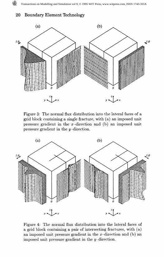
parallel to the zz-plane and connecting the grid block faces parallel tothe yz-plane. (In all our fracture realizations the fractures connect thegrid block faces parallel to the xy-plane). The trace of the fracture in thexy-plane is a line segment from the point (0.0,0.4) to the point (1.0,0.4).In figure 3(a) we give a plot of the normal fluxes on the lateral faces ofthe grid block for the solution corresponding to a unit pressure gradient inthe x-direction. In figure 3(b) we depict the normal fluxes for the solutioncorresponding to a unit pressure gradient in the y-direction. A 4 x 4 meshon each surface was used in the boundary element method for both cases.From the figures we see that in this geometry the fracture has no effect onthe solution when the pressure gradient is orthogonal to the fracture plane.However, when the pressure gradient is parallel to the fracture plane theflow is strongly enhanced near the fracture, i.e., more fluid can flow alongthe higher conductivity pathway corresponding to the fracture. Also, forthis case there is a very small nonzero normal flux on the grid block facesparallel to the fracture. As expected from symmetry considerations of theperiodic array (for which we are solving the flow in one cell) the averageflux over this face is zero. The small nonzero flux values result from theasymmetric position of the fracture in the grid block. Using the averageflux values the effective permeability of this fractured grid block is

2.69503 0.00000 0.00000 \0.00000 1.00000 0.00000 . (18)0.00000 0.00000 2.69503 /

This shows that in the directions parallel to the fracture plane there is anincrease in the conductivity due to the presence of the fracture.

In our second example we have a pair of intersecting fractures. Thetrace of the first fracture in the xy-plane is a line segment joining thepoint (0.3,0.4) to the point (1.0,0.4). The trace of the second fracture inthe xy-plane is a line segment joining the points (0.6,0.0) and (0.6,0.5).



Using a 4 x 4 mesh in the boundary element method leads to the followingeffective permeability tensor

(1.53132 0.01026 0.00000 \0.01145 1.22460 0.00000 . (19)0.00000 0.00000 3.04115 /

Repeating the calculation with an 8x8 mesh on each surface yields thepermeability tensor

1.47805 0.01777 0.00000 \0.01442 1.22248 0.00000 . (20)0.00000 0.00000 3.32460 /

In figure 4 we depict the flux distribution flowing into the lateral faces ofthe grid block for unit pressure gradients in the x and y directions. Theflux plots in figure 4 were obtained from the solution corresponding to the8x8 mesh. As was the case in figure 3, the plots in figure 4 also showthat there are high flow pathways corresponding to the fracture locations.The asymmetry in the geometry leads to flow in the direction orthogonalto the pressure gradient. This manifests itself in the effective conductivitytensor as nonzero off-diagonal components.

5 Conclusions

We have described a model for representing a fractured reservoir and amethod for computing the effective permeability of blocks from such areservoir. In our model the fractures are represented by planes and theflow in each fracture is treated as 2-dimensional flow in a plane. Flowbetween the fractures and the porous matrix is represented by a planarsource distribution for flow in the matrix and by an equivalent planar sinkdistribution for flow in the fractures. The essential feature of this modelis that the fractures act as high flow conduits within the matrix. Themathematical formulation, corresponding to this model, is solved usingthe boundary element method for a fractured cube subject to periodicboundary conditions. The effective permeability tensor, associated withthe block, is deduced from the average fluid velocities across the end faces.

Acknowledgements

The work presented in this paper was supported jointly by the StrategicResearch Department at Chevron Petroleum Technology Company andby the Gas Research Institute (Contract No. 5094-210-3050).



References

1 Kazemi, H., Merril, L.S. Jr., Porterfield, K.L. & Zeman, P.R. Numer-ical Simulation of Water-Oil Flow in Naturally Fractured Reservoirs,Society of Petroleum Engineers Journal 1976, pp 317-326

2 Pruess, K. & Narasimhan, T.N. A Practical Method for ModelingFluid and Heat Flow in Fractured Porous Media, Society of PetroleumEngineers Journal 1985, pp 14-26

3 Van Golf-Racht, T.D. Fundamentals of Fractured Reservoir Engineer-ing, Elsevier, 1982

4 Laubach, S.E. Fracture Patterns in Low Permeability Sandstone GasReservoir Rocks in the Rocky Mountain Region, paper SPE 21853presented at the Rocky Mountain Regional Meeting and Low Perme-ability Reservoirs Symposium, April, 1991, Denver

5 Lorenz, J.C. & Hill, R.E. Subsurface Fracture Spacing: Comparison ofInferences from Slant/Horizontal Core and Vertical Core in MesaverdeReservoirs, paper SPE 21877 presented at the Rocky Mountain Re-gional Meeting and Low Permeability Reservoirs Symposium, April,1991, Denver

6 Long, J.C.S., Gilmour, P. & Witherspoon, P.A. A Model For SteadyFluid Flow in Random Three-Dimensional Networks of Disc-ShapedFractures Water Resources Research, 1985, 21, pp 1105-1115

7 Homsy, G.M. Viscous Fingering in Porous Media, Annual Review ofFluid Mechanics, 1987, 19, pp 271-311

8 Durlofsky, L.J. Numerical Calculation of Equivalent Grid Block Per-meability Tensors for Heterogeneous Porous Media, Water ResourcesResearch, 1991, 27, pp 699-708

9 Amaziane, B. & Bourgeat, A. Effective Behavior of Two-Phase Flowin Heterogeneous Reservoirs, in Numerical Simulation in Oil Recov-ery, ed M.F. Wheeler, pp 1-22, Springer-Verlag, 1988

10 King, P.R. The Use of Renormalization for Calculating Effective Per-meability, Transport in Porous Media, 1989, 4, pp 37-58

11 Brebbia, C.A. The Boundary Element Method for Engineers, PentechPress, 1978

12 Krahenbiihl, L., Nicolas, A. & Nicolas, L. PHI3D: A Graphic Interac-tive Package for Three-Dimensional Fields Computation, in Betech86 (ed J.J. Connor & C.A. Brebbia), pp. 33-43, Proceedings of the 2ndBoundary Element Technology Conference, Massachusetts Institute ofTechnology, USA, June 1986, Computational Mechanics Publications1986



(a) ^ (b)

Figure 3: The normal fiux distribution into the lateral faces of agrid block containing a single fracture, with (a) an imposed unitpressure gradient in the x-direction and (b) an imposed unitpressure gradient in the ̂ -direction.

(a)

Figure 4: The normal flux distribution into the lateral faces ofa grid block containing a pair of intersecting fractures, with (a)an imposed unit pressure gradient in the ̂ -direction and (b) animposed unit pressure gradient in the ̂ /-direction.


modeling of fractured reservoirs using the boundary element method

Documents