modeling of fiber-reinforced plastics …. reclusado, s. nagasawa 1 introduction injection molded...

ECCOMAS Congress 2016 VII European Congress on Computational Methods in Applied Sciences and Engineering

M. Papadrakakis, V. Papadopoulos, G. Stefanou, V. Plevris (eds.) Crete Island, Greece, 5–10 June 2016

MODELING OF FIBER-REINFORCED PLASTICS TAKING INTO ACCOUNT THE MANUFACTURING PROCESS

Cherry Ann T. Reclusado1, Sumito Nagasawa2

1 Fraunhofer Institute for High-Speed Dynamics, Ernst-Mach-Institut, EMI Eckerstraße 4, 79104 Freiburg, Germany [email protected]

2 Fuji Heavy Industries Ltd. 1-1 Subaru-cho, Ota-shi, 373-8555 Gunma, Japan

[email protected]

Keywords: Integrative simulation, process and structural simulation, crash simulation, fiber-reinforced plastics, orientation tensor, degree of anisotropy

Abstract: In a joint project of the EMI and Fuji Heavy Industries Ltd. a method for the mod-eling of fiber-reinforced plastics was developed, taking into account the manufacturing pro-cess. Within this study, an approach for a detailed characterization and modeling of a fiber reinforced plastic is described and presented by the example of a PPGF30 material. The characterization of the orientation dependent material behavior includes tensile tests at dif-ferent strain rates as well as tensile-unloading, compression and shear tests in 0°-, 45°- and 90°-direction. Also, quasi-static and dynamic three-point bending tests are performed and act as validation tests for the simulation model. For further validation of the method and to eval-uate the simulation model’s approximation to reality, dynamic three-point bending tests are performed on a component with a ribbed structure. Regarding the modeling of the mechanical behavior, the fiber orientation distribution is taken into account by means of injection mold-ing simulations, both in the sample plate and the component. These simulations provide in-formation about the orientation state at discrete material points in terms of an orientation tensor. By means of the eigenvalues and the respective eigenvectors of the orientation tensors, the degree of anisotropy and the principle fiber direction are defined. However, the degree of anisotropy is considered in a gradual manner by defining several material classes, each cov-ering different ranges of the greatest eigenvalue. This is a very time consuming approach, be-cause for each material class, one set of parameters has to be calibrated iteratively. The impact of considering the degree of anisotropy on the simulation results is therefore investi-gated as well. Another crucial aspect within this work is the development of a program to au-tomatically translate and map the injection molding simulation results to appropriate variables in the structural simulation model. Furthermore, high-resolution CT-scans of the sample plate and the component are created in order to perform a fiber analysis of the real material and hence to verify the injection molding simulation results.

C.A. Reclusado, S. Nagasawa

1 INTRODUCTION

Injection molded glass fiber-reinforced plastics (GFRP) play an important role as modern lightweight construction materials, used for example for interior or exterior parts in the auto-motive industry. Those materials combine high-strength glass fibers with a shaping polymer matrix. A suitable distribution of the fiber orientation and the degree of anisotropy within a component can contribute positively to its resistance against deformations. Furthermore, the injection molding process allows for a functional integration and the production of ribbed structures, which lead to an additional stiffness of thin-walled components. Although contin-uous fiber-reinforced plastics with a selective orientation of the fiber strands can achieve even higher stiffnesses, the use of injection molded plastics is preferred due to lower manufacturing costs and cycle times. On the other hand, high development costs and times have to be con-sidered. Especially the complex distribution of the fibers in injection molded components complicates the prediction of material properties and may require the cost-intensive manufac-turing of prototypes. Often numerical simulations are used to predict the material behavior. Injection molding simulations (e.g. using Moldflow) allow for the calculation of fiber distri-butions, orientations and joint lines whereas structural simulations (e.g. using LS-DYNA) are used to calculate the mechanical behavior of a component. For such a structural simulation material parameters are needed which have to be determined in characterization tests. The consideration of all those results from injection molding and structural simulations as well as from the characterization tests is called »integrative simulation«. As in the conventional ap-proach, the characterization tests are simulated and the material parameters as well as the structural model are validated by comparing stress-strain- and force-displacement-curves. For an integrative simulation, in addition, process-related parameters like fiber orientation and degree of anisotropy are included in the structural model.

Within this study the thorough investigation and modeling of a GFRP, subjected to dynam-ic loading, are presented by the example of a PPGF30 material, a long glass fiber reinforced thermoplastic (LGFRP). The characterization tests for obtaining the material parameters for modeling the orientation dependent material behavior include tensile tests at different strain rates, as well as tensile-unloading, compression and shear tests on specimens extracted paral-lel (0°-direction), perpendicular (90°-direction) and in 45°-direction to the main flow direc-tion in the sample plate. When determining the material parameters, the fiber distribution is taken into account by means of an injection molding simulation. This simulation provides in-formation about the orientation state at discrete material points in terms of an orientation ten-sor. By means of the eigenvalues and the respective eigenvectors of the orientation tensors the degree of anisotropy and the principle fiber direction are defined. Similar to the described ap-proach in [1] several material classes are declared to cover different degrees of anisotropy and for each material class one MAT_108 material card [3], available in the finite element code LS-DYNA, is generated. Furthermore, the material cards are assigned by means of the key-word ELEMENT_SHELL_COMPOSITE [2]. The calibration of the MAT_108 material cards is based on the results from the dynamic tensile tests at nominal strain rate of 100/s. To model the failure behavior one MAT_ADD_EROSION card is assigned to each MAT_108 material card.

The validation of the parameters is done by comparing the stress-strain- and force-displacement-curves of the structural simulation and the experiments. In addition, to evaluate the predictive power of the prepared models and the introduced approach to incorporate pro-cess simulation results in the modeling of the mechanical behavior of the PPGF30 material, dynamic three-point bending tests and a structural simulation of these tests are performed us-ing a component with a ribbed structure.


Another crucial aspect within this work is the development of a program to automatically map the injection molding simulation results to appropriate variables in the structural simula-tion model. This mapping tool not only translates information about the orientation state, but it also enables to overcome the mesh inconsistency between the tetrahedron mesh of the injec-tion molding simulation and the shell mesh of the structural simulation. Furthermore, high-resolution CT-scans of selected regions of the sample plate and the component are created to validate the injection molding simulation results.

2 INTEGRATIVE SIMULATION

As already mentioned the use of injection molded GFRP enables the development of high-strength and very stiff components, but it comes with a complex material behavior. Different fiber orientation distributions, which make it difficult to predict the principle direction and the degree of anisotropy, can arise in various positions in the component. In addition, the outer and inner layers of a thin walled component can show a varying orientation distribution. While the fibers in the outer layers are likely oriented in the flow direction, the fibers in the inner layers are more deviated – in the most extreme case perpendicular to the flow direction. The varying fiber orientation distribution, which results due to the flow of the viscous fiber-reinforced plastic melt while injected in the cavity, represents a challenge for the structural simulation, because as one can conclude it is no longer sufficient to simply assume the princi-pal fiber alignment and degree of anisotropy. To fully exploit the advantages of a GFRP the fiber orientation distribution needs to be considered both in the finished component and the sample plate, from which the specimens for the characterization tests are extracted. One way to detect the fiber orientation within a component is to make CT-scans, but the disadvantage of this technique is that the component has to be manufactured first. Alternatively, a process simulation can be performed. By simulating the injection molding process of the GFRP com-ponent the filling of the cavity and the orientation state of the final part can be predicted at discrete points. Incorporating quantities from a process simulation in the material modeling and structural simulation is called »integrative simulation«. The methodology of how the in-tegrative simulation is realized in the present work is illustrated in Figure 1.

Figure 1: Methodology of the realized integrative simulation.


Centerpiece of this methodology is a mapping-tool which automatically translates the in-formation about the fiber orientation and distribution and which also resolves the mesh incon-sistencies caused by different discretizations of the geometry used in the injection molding and in the structural simulation. In order to model different degrees of anisotropy, several ma-terial classes are introduced. For each material class, a material card is calibrated, for which the elastic constants are determined using a method described by Advani and Tucker [4]. The plastic parameters, which are the same for all material classes/cards, are identified by an op-timization software.

In case of injection molded GFRP the orientation tensor is calculated at discrete material points in the process simulation. Strictly speaking the second order orientation tensor aij is calculated, which can be described as a symmetric 3x3 matrix. In order to visualize aij, its ei-genvalues and eigenvectors are generated by performing a principal axis transformation. The eigenvectors display the principal directions of the fiber alignment, while the eigenvalues in-dicate the fiber orientation distribution, ranging from 0 to 1, in the corresponding direction. The sum of all three eigenvalues is equal to 1. By displaying the eigenvectors and eigenvalues in a Cartesian coordinate system an orientation ellipsoid can be defined (see Figure 2).

.

→Eigenvectors:Eigenvalues:

Figure 2: Orientation ellipsoid stretched from the eigenvectors and eigenvalues of the second order orientation tensor.

It is very unlikely that the fibers within one finite volume in the component are aligned in one direction. Instead the fibers are randomly deviated to a greater or lesser extent and lead to varying degrees of anisotropy and hence to varying shapes of the orientation ellipsoid.

3 BASIC PRINCIPLE OF THE DEVELOPED MAPPING TOOL

The flow-chart describing the mapping tool is shown in Figure 3. After importing the shell element model, the tetrahedral element model, and the orientation tensors a calculation algo-rithm is started. Those orientation tensors, introduced by Advani and Tucker, have been de-termined by an injection molding simulation for the tetrahedral elements. The mapping tool now divides the shell elements into several layers and calculates the space that would be oc-cupied by each layer based on its thickness. Afterwards, the tetrahedral elements correspond-ing to this space are assigned and averaged orientation tensors are calculated for each layer of the shell elements, taking into account its volume fraction. The eigenvalues (λ1, λ2, λ3) and eigenvectors (e1, e2, e3) of the orientation tensors are determined by a principal axis transfor-mation. It is assumed that only the largest eigenvalue λ1 and its eigenvector e1 are relevant for the calculation of the necessary parameters for the structural simulation composite shell ele-ment model. The vector λ1e1 of each layer is now projected onto the shell element in order to eliminate its component normal to the element surface. The rotation angle, which rotates the fiber direction of the local shell element coordinate system in the direction of the projected


eigenvector, is directly entered into the composite shell element model. Depending on the length of the projected eigenvector, a material class is assigned to each layer. The number of the corresponding material card is also entered into the composite shell element model.

Figure 3: Flow-chart of the developed mapping-tool.

4 DEGREE OF ANISOTROPY

For the definition of the degree of anisotropy, several material classes have to be declared at first. As mentioned before the sum of all three eigenvalues equals 1. In the present study a long fiber reinforced thermoplastic is investigated and the probability of fibers oriented in thickness direction is very low. Therefore, it is assumed that the eigenvectors corresponding to the largest and second largest eigenvalue are mainly aligned parallel to the shell plane. The classification of the degree of anisotropy can simply be done by defining ranges of the largest eigenvalue and each range is represented by a material class. Because the sum of all eigenval-ues is 1 and the eigenvalue in the thickness direction is assumed to be 0, the minimum value of the largest eigenvalue is 0.5. In the present study three material classes are defined with the background that a composite made of a GFRP material is parted in two outer layers, two tran-sition layers and one central layer (see Figure 4). An example for a range specification of the largest eigenvalue and the assignment of the corresponding material classes is presented in Figure 5.

Figure 4: Significant layers: two outer layers (1 and 5), two transition layers (2 and 4), and one central layer (3)

within a composite.


Figure 5: Material classification (degree of anisotropy) used for the material modeling.

5 MATERIAL MODELING

Advani and Tucker [4] proposed an approach to calculate the engineering constants of a material with arbitrary fiber distribution by means of the engineering constants in the uni-directional state. However, from the tensile tests one obtains a combined Young‘s and shear modulus because the fiber distribution in the tested specimens are arbitrary. The approach proposed by Advani and Tucker is therefore reversed. Judging from the injection molding simulation results of the sample plate the central layer is of material class 3 and the outer and transition layers of material class 2. Also from the CT-scans no significant difference between the outer and transition layers can be observed. As an example the CT-scan of a specimen lo-cated in the central part of a tensile specimen aligned in 0°-direction is shown in Figure 6 a. The extraction position from the sample plate and the location of the presented CT-scan can be seen in Figure 6 b. It can be observed, that the thickness of the central layer is approxi-mately one fifth of the total thickness. Hence, specifying five layers over the thickness, with each layer having a thickness of one fifth of the total thickness, can be justified.

a)

b)

Figure 6: CT-scan of a specimen extracted from position A on the sample plate.

To calculate the Young’s and shear moduli for the three specified material classes the Young’s moduli and the in-plane shear modulus determined from tensile and shear tests in 0°- and 90°-direction are used.


It is assumed, that the Young’s moduli and the in-plane shear modulus are composed as follows:

° 1 , (1)

° 1 , (2)

°/ ° 1 , (3)

with η = 0.2. The upper index indicates the material class and the lower index indicates the mainly in-

volved direction of the orthotropic material. By means of the Young‘s moduli and the shear modulus from the characterization tests the

engineering constants of the uni-directional material is calculated using an optimization algo-rithm. In the uni-directional state all fibers are aligned in one direction and the largest eigen-value is λ1 = 1. For material classes 1, 2 and 3 values of λ1

(1) = 0.9, λ1(2) = 0.7 and λ1

(3) = 0.5 are used. With the normalized moduli of E0° = 3.74 MPa, E90° = 2.05 MPa and G0°/90° = 1 MPa the normalized engineering constants for each defined material class are obtained as shown in Table 1. Because the optimization algorithm could not calculate reasonable values for the Poisson ratios, the values of ν12 = 0.34, ν23 = 0.2 and ν31 = 0.21 are assumed.

Material class λ1 E1 [MPa] E2 [MPa] G12 [MPa] 1 0.9 6.20 1.14 0.61 2 0.7 4.01 1.90 0.98 3 0.5 2.64 2.64 1.10

Table 1: Engineering constants for the three defined material classes.

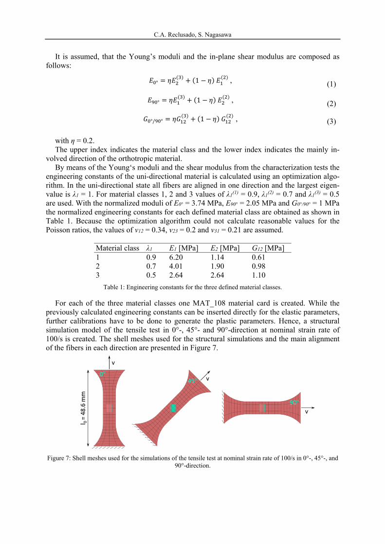
For each of the three material classes one MAT_108 material card is created. While the previously calculated engineering constants can be inserted directly for the elastic parameters, further calibrations have to be done to generate the plastic parameters. Hence, a structural simulation model of the tensile test in 0°-, 45°- and 90°-direction at nominal strain rate of 100/s is created. The shell meshes used for the structural simulations and the main alignment of the fibers in each direction are presented in Figure 7.

Figure 7: Shell meshes used for the simulations of the tensile test at nominal strain rate of 100/s in 0°-, 45°-, and

90°-direction.


To account for the fiber orientation distribution, the injection molding simulation result of the sample plate is mapped to the shell mesh of the structural simulation models.

By means of the software LS-OPT by LS-DYNA the plastic parameters are calibrated and the same values are used for all material cards. For this the respective smooth force-displacement curves of the tensile tests in 0°-, 45°-, and 90°-direction at a nominal strain rate of 100/s (haul-off speed of 9720 mm/s) are compared to the simulated curves.

During the calibration of the plastic parameters with LS-OPT the elastic parameters for each material class are held constant.

Failure is modeled by assigning one MAT_ADD_EROSION card to each MAT_108 mate-rial card, whereby the defined failure criteria are identical for all three MAT_ADD_EROSION cards. The failure parameters are obtained from the tensile tests at a nominal strain rate of 100/s. As failure criteria a value for the maximum stress and maximum strain is inserted. The value for the maximum strain is the average failure strain from the ten-sile tests at haul-off speed of 9720 mm/s in 90°-direction. The maximum stress is generated by reverse engineering. To prevent the failure of the integration points under compression loading a value of -20 MPa (pressure is negative for tensile) for the minimum pressure is in-serted as well. Variable NCS (number of failure conditions to satisfy before failure occurs) is set to 2. In this manner failure occurs if two failure criteria are met, e.g. maximum stress and minimum pressure.

As can be seen in Figure 8 and Figure 9 the force-displacement and stress-strain curves from the tensile tests at haul-off speed of 9720 mm/s in 0°-, 45°-, and 90°-direction can be represented well with the generated elastic and yield parameters. Also, failure can be simulat-ed sufficiently.

Figure 8: Comparison of the simulated and experimentally determined force-displacement curves from the ten-

sile tests at a haul-off speed of 9720 mm/s in 0°-, 45°-, and 90°-direction.

Fo

rce

Displacement

Tensile tests at 9720 mm/s 0° 45° 90°

Smooth fitting 0° 45° 90°

Simulation 0° 45° 90°


Figure 9: Comparison of the simulated and experimentally determined stress-strain curves from the tensile tests

at a haul-off speed of 9720 mm/s in 0°-, 45°-, and 90°-direction.

6 VALIDATION OF THE METHOD

To validate the developed approach comprising the mapping tool, the calculation of engi-neering constants for various degrees of anisotropy, and the generation of the material cards, three-point bending tests are performed on a component part made of a PPGF30 material. The test set-up on the servo-hydraulic high strain rate testing machine is shown in Figure 10. For better tracking of the deformation the edges of the components are painted with a white mark-er. Furthermore, a stop on the left side and on the back is used to align the components and thus to minimize the scatter.

Figure 10: Three-point bending test set-up on the VHS testing machine.

True

str

ess

Local true strain

Tensile tests at 9720 mm/s 0° 45° 90°

Average 0° 45° 90°

Simulation 0° 45° 90°


Due to the draft angle the outer ribs of the component form a trapezoid and also the thick-ness of the ribs increases in the direction of the bottom. The trapezoidal shape is considered in the simulation model and the component is aligned accordingly. The simulation model of the three-point bending test is shown in Figure 11. Here it can be seen, that the ribs are divided in 19 sections, or 19 shell element rows, over the height. To represent the varying thickness of the ribs, the average thickness of each section is assigned to the shell elements within the sec-tions.

Figure 11: Simulation model of the three-point bending test.

The generated structural simulation model of the component consists of 8155 shell ele-ments and 8200 nodes and the calculations are performed with LS-DYNA version R7.1.1 re-vision 88541. The edge length of the elements is approximately 2 mm and fully integrated shell elements (ELFORM = 16) are used. The supports and the fin are represented by surfaces and are defined as rigid bodies. While the supports move upwards, the fin is fixed. The veloci-ty boundary condition assigned to the supports is derived from the velocity of the piston dur-ing the test. Between the component and the rigid bodies, a contact is defined, with an assumed static friction value of FS = 0.2, a dynamic friction value of FD = 0.15 and a decay of DC = 0.5. Also a self-contact is defined for the component and the same friction values as mentioned before are assumed.

The force-displacement curves of the five valid tests and the simulation are shown in Fig-ure 12. The progressions of the test curves are similar and only a small scatter can be ob-served. It is assumed that the large scatter at larger displacements can be explained by different post failure behavior of the component in each test. Due to the oscillations and the fact, that only the front side of the component can be observed it is difficult to trace variations of the force signal to occurring deformations of the part. However, four pictures, which show the deformation of the components at significant incidents during the tests, are selected exem-plarily from Test 1. The selected pictures and the associated moment in the force-displacement curve (marked as blue rectangles in the diagram) of the experiment and the sim-ulation are presented in Figure 12. The first picture shows the initial contact between the fin and the part. The total failure of the upper rib right below the fin can be seen in the second picture. After a drop of the force-displacement curve the force increases again. As can be seen in the third picture, this is where the edge between the left transverse and left upper rib strikes the fin. The last picture shows the total failure of the lower rib, but due to the varying post failure behavior in each test this picture is of no significance.

The simulation result agrees well with the experiments regarding the curve progression, the force level and also the deformation behavior and thus the predictive power of the method can be illustrated. However, it should be noted that the simulation result strongly depends on the number of failed integration points prior to element deletion NUMFIP in the


MAT_ADD_EROSION card and on the friction values in the contact definitions. For the pre-sent simulation the previously mentioned contact friction values are inserted and for NUMFIP a value of -105 (When NUMFIP < -100, elements erode when |NUMFIP|-100 integration points fail. Also, for NUMFIP < -100, the stress at an integration point immediately drops to zero when failure is detected at that integration point) is applied.

1) 2)

3) 4)

Figure 12: Simulated and experimentally determined force-displacement curves from the dynamic three-point

bending tests and pictures of significant incidents during the test and simulation.

7 FIBER ANALYSIS BASED ON CT-SCANS

To further improve the results of an integrative simulation, the injection molding simula-tion results have to be validated. For this, the fiber orientation in the real material has to be determined via CT-scans and a fiber analysis. Such a fiber analysis was done using the soft-ware VGStudio MAX 2.2. The exemplary result of a fiber analysis of the investigated

432

Fo

rce

Displacement

Test 1 Test 2 Test 3 Test 4 Test 5 Simulation

1


PPGF30 material is shown in Figure 13 together with the fiber orientations determined from the injection molding simulation. On the bottom, cross sectional views of the material with thickness t are shown. The different colors in the middle layer of the cross sectional view of the fiber analysis indicate a different orientation of the fibers in this layer compared to the outer layers. Sectional views through the middle layer (A) and the outer layer (B) confirm this result: The fibers in the outer layer are oriented mainly in flow direction (0°), whereas in the middle layer the fibers are deflected from the flow direction by angles between 40°-60°. The same can be seen in the results from the injection molding simulation. However, the deflec-tion of the fibers in the middle layer is much lower (10°-15°) than in the real material.

Figure 13: Fiber analysis of an injection molded fiber-reinforced plastic based on CT-scans compared to an in-

jection molding simulation.

8 IMPACT OF CONSIDERUNG THE DEGREE OF ANISOTROPY

In the presented methodology of an integrative simulation the degree of anisotropy is con-sidered in a gradual manner by defining several material classes, each covering different ranges of the greatest eigenvalue. But considering the degree of anisotropy in this way is a rather time consuming approach, because for each material class, one set of parameters has to be calibrated iteratively using the software LS-OPT. Due to this fact it is reasonable to ask about the advantages of considering the degree of anisotropy compared to less complex mod-elling approaches. To answer this, the effect of considering the degree of anisotropy was fur-ther investigated by performing two additional simulations of the dynamic three-point bending test. In the first simulation only the fiber orientation was considered. Furthermore, the values for the elastic and plastic parameters in the longitudinal and transversal material direction are derived solely from the dynamic tensile tests in 0°- and 90°-direction, respective-ly. In the second simulation an isotropic material behavior was used. For both simulations all other parameters, e.g. friction values, are adopted from the structural simulation model pre-sented in section 6.


In Figure 14 the simulation considering only the fiber direction, and in Figure 15 the simu-lation using an isotropic material behavior is compared to the experiment and the simulation considering the degree of anisotropy.

Figure 14: Comparison of the simulation considering only the fiber orientation with the simulation considering the fiber orientation and the degree of anisotropy.

Failure upper rib

Total failure

Fo

rce

Displacement

Test 1 Test 2 Test 3 Test 4 Test 5

Simulation Consid. aniso. Only fiber orient.


Figure 15: Comparison of the simulation using an isotropic material behavior with the simulation considering the

fiber orientation and the degree of anisotropy.

Regarding the initial curve progression and the force level, both simulations show equally good agreement with the experiment. But in contrast to the experiment in the simulation con-sidering only the fiber orientation the upper part of the bottom wall remains intact longer. In addition, the upper rib is not bent. For this reason the force increases significantly and the to-tal failure occurs much earlier than in the experiments. The same can be observed in the simu-lation using an isotropic material behavior. Here the upper part of the bottom wall fails in a larger region, but the edge between the upper and bottom wall is not impressed. Latter can be observed in all other simulations and the experiment.

In conclusion the simulation considering the degree of anisotropy shows the best agree-ment with the experiment throughout the entire length of the test, regarding the curve progres-

Failure upper rib

Total failureFor

ce

Displacement

Test 1 Test 2 Test 3 Test 4 Test 5

Simulation Consid. aniso. Isotr. mat. behav.


sion, the force level and the deformation behavior. When considering only the fiber orienta-tion or using an isotropic material behavior, the deformation behavior cannot be represented well and in the present study failure occurs too early. However, regarding the curve progres-sion and force level only, the simulations show comparable good results.

9 CONCLUSIONS

The mechanical behavior of a long fiber reinforced thermoplastic material is character-ized and modeled in detail by taking into account the fiber orientation distribution within the material

For this purpose, the fiber distribution is thoroughly investigated by performing injection molding simulations and CT-scans of a ribbed component and a sample plate, from which the specimens for the characterization tests are extracted. Together with the results of injection molding simulations, characterization tests and additional structural simula-tions of the characterization tests, parameters for the material modeling are identified.

In the present study this approach, also known as integrative simulation, is shown by means of a PPGF30 material, a long glass fiber reinforced thermoplastic. But it should be generally applicable for all long fiber reinforced plastics.

The characterization of the orientation dependent material behavior includes tensile tests at different strain rates as well as tensile-unloading, compression and shear tests in 0°-, 45°-, and 90°-direction

Injection molding simulations of the sample plate and the component have been carried out and provide information about the fiber orientation state in terms of the second order orientation tensor

The largest eigenvalue of the orientation tensor is a measure for the degree of anisotropy and the associated eigenvector delivers the principle fiber direction. The classification of the degree of anisotropy is made in terms of several material classes, which cover differ-ent ranges of the largest eigenvalue. For each material class one MAT_108 material card is defined. The determination of the material parameters is done in two steps. At first the elastic parameters are calculated by means of an optimization algorithm. The underlying equation is derived from an approach proposed by Advani and Tucker to calculate the engineering constants of a material with arbitrary fiber distribution by means of the engi-neering constants in the uni-directional state. In a second step a structural simulation model of the tensile tests at haul-off speed of 9720 mm/s in 0°-, 45°-, and 90°-direction is created.

In order to also account for the fiber orientation state in the material a mapping tool is developed, which automatically calculates quantities from the injection molding simula-tion results and integrates them in the structural simulation model. With this mapping tool the fiber orientation and the material card is specified for each layer of the shell ele-ment meshes of the tensile specimens with the keyword ELEMENT_SHELL_COMPOSITE in LS-DYNA.

The calibration of the plastic material parameters is carried out using the software LS-OPT. In addition, the failure behavior is modeled by assigning one MAT_ADD_EROSION card to each MAT_108 material card. The failure parameters are generated by reverse engineering.


With the elastic, plastic and failure parameters obtained in this way the force-displacement and stress-strain curves of the tensile tests at haul-off speed of 9720 mm/s can be represented well in 0°-, 45°-, and 90°-direction.

For further validation of the mapping tool and the generated material parameters dynamic three-point bending tests are performed on a ribbed component. Judging from the force-displacement curves and the analysis of the deformation of the component the experi-ments can be represented well by the generated structural simulation model.

CT-scans are made from selected areas of the sample plate and the component. Based on the data obtained from these CT-scans fiber analyses are performed and serve as valida-tion of the injection molding simulation results.

The impact of considering the degree of anisotropy was investigated in detail and a com-parison with a simulation considering only the fiber orientation and a simulation using an isotropic material behavior was made. The simulation considering the degree of anisotro-py showed the best agreement with the experiment throughout the entire length of the test, regarding the curve progression, the force level and the deformation behavior. The other two simulations could not represent the deformation behavior well, but regarding the curve progression and force level, comparable good results can be shown.

10 ACKNOWLEDGEMENT

This work was developed in coorperation between the EMI and Fuji Heavy Industries Ltd. and the authors wish to acknowledge the support and contribution of all project partners.

REFERENCES

[1] G. Gruber, A. Haimerl, S. Wartzack, Consideration of Orientation Properties of Short Fiber Reinforced Polymers within Early Design Steps. 12th International LS-DYNA Conference, 2012.

[2] Livermore Software Technology Cooperation, Livermore, LS-DYNA Keyword User’s Manual: Volume I, Version R7.1., Cal., May, 2014.

[3] Livermore Software Technology Cooperation, Livermore, LS-DYNA Keyword User’s Manual: Volume II Material Models, Version R7.1., Cal., May, 2014.

[4] S.G. Advani, C.L. Tucker, The Use of Tensors to Describe and Predict Fiber Orienta-tion in Short Fiber Composites. Journal of Rheology, 31(8), 751-784, 1987.

modeling of fiber-reinforced plastics …. reclusado, s. nagasawa 1 introduction injection molded...

Documents