modeling networks a dissertation - the …i.stanford.edu/~mykim/pub/myunghwankimthesis.pdfdous...
TRANSCRIPT

MODELING NETWORKS
WITH AUXILIARY INFORMATION
A DISSERTATION
SUBMITTED TO THE DEPARTMENT OF ELECTRICAL
ENGINEERING
AND THE COMMITTEE ON GRADUATE STUDIES
OF STANFORD UNIVERSITY
IN PARTIAL FULFILLMENT OF THE REQUIREMENTS
FOR THE DEGREE OF
DOCTOR OF PHILOSOPHY
Myunghwan Kim
August 2014

iv

Abstract
Networks provide a powerful tool for representing social, technological, and biological
systems. The study of networks has focused on developing models that either analytically
show the emergence of global structural properties in networks or statistically perform
inference tasks, such as link prediction, on given network data. This thesis presents a model
of networks that not only gives rise to realistic networks with the global structural properties
but also permits statistical inference for given network data. Under the proposed model, we
prove many structural properties commonly found in real-world networks, such as heavy-
tailed degree distributions and small diameters. We also develop a statistical inference
algorithm that fits the model to given network data and represents common linking patterns
through our model.
A network is often associated with auxiliary information, such as node features or tem-
poral information about node and link creations and deletions. This thesis also proposes
models of networks with such auxiliary information so that the models capture the relation-
ships between given network links and the auxiliary information. In the second part of the
thesis, we propose a model that allows for relationships between given node features and
network links. We develop a fitting algorithm that identifies which node features are rele-
vant to network links and how the node features affect the formation of the links. By fitting
our model to given network links and node features, our model improves performance for
various prediction tasks compared to baseline models.
Finally, we develop a model for dynamic networks by considering two notions of dy-
namics: the birth and death of each group of nodes, and each individual node’s behavior
of joining or leaving some node groups over time. By embedding these two dynamics into
the model, we can achieve the interpretable representation of network dynamics as well as
the predictive power of inferring missing links or forecasting future networks.
v

vi

Acknowledgements
Thanks to so many people around me, my doctoral thesis could be successfully finished. It
is thus great pleasure to express my sincere gratitude to everyone.
First of all, it is my honor and luck to have worked with Professor Jure Leskovec. I can
never appreciate him enough. As an academic advisor and mentor, he guided, supported,
and encouraged me throughout the journey for my doctorate at Stanford University. I owed
an inestimable debt to him for my professional and personal development.
I also thank my thesis and oral examination committee members, Professor Hector
Garcia-Molina, Professor Art Owen, Professor Andrea Montanari, and Rok Sosic for their
help and valuable comments.
I thank all my collaborators (Professor Anthony Bonato, Professor David F. Gleich,
Nish Parikh, Professor Paweł Prałat, Sam Shah, Roshan Sumbaly, Neel Sundaresan, Amanda
Tian, and Professor Stephen J. Young in alphabetical order). In particular, I had two won-
derful summers on collaborating with them at eBay Research Labs, LinkedIn Corporation,
and the MITACS workshop. Throughout the collaboration outside Stanford, I could learn
different professional world and obtain motivation and inspiration about research.
I gratefully appreciate SNAP group members (Ashton Anderson, Christina Brandt,
Justin Cheng, Cristian Danescu-Niculescu-Mizil, Andrej Krevl, Himabindu Lakkaraju, Ju-
lian McAuley, Seth A. Myers, Yonathan Perez, Dafna Shahaf, Bob West, and Jaewon Yang
in alphabetical order). It was great experience to both social and professional weekly group
meeting and share considerable intellect with them there. I would like to express a special
thank to Jaewon for sharing information and intellect, giving great feedback on my re-
search, and having lunch and beer time together.
vii

I also thank Infolab group members and alumni (Professor Jennifer Widom, Profes-
sor Jeffrey D. Ullman, Aditya G. Parameswaran, Hyunjung Park, Steven Whang, Petros
Venetis, and many others) for giving valuable feedback and advice for my next career. A
special thank goes to Hyunjung Park because he introduced this amazing group to me,
mentored me for career and life at Stanford, and led me to many fun places. I also would
like to thank Marianne Siroker for her administration.
My special thanks go to many Korean friends. First, I sincerely thank my lunch and
coffee mates, Youngsik Kim, Sunghee Park, Sanghoek Kim, and Kietae Kwon. Lunch and
coffee time with them always refreshed me for better productivity and sometimes became
discussion time with non-experts in my area. Second, SSHS friends deserve my tremen-
dous gratitude: Hyoungjoon Ahn, Sungwook Chang, Hyungil Chae, Bongsoo Kyung, Jae-
hoo Lee, Taejoon Seok, Jaewon Shim, Hyungchai Park, John Hong, and Gyuwon Hwang.
Third, I also appreciate members of my basketball club and squash club. It was always
great to have fun with all the Korean friends. Moreover, they all formed amazing over-
lapping social circles so that my ego-network could become a wonderful dataset for my
research.
I would like to show a special thank to Louis Kavanau. It was very fortunate for me
to meet him through the English-In-Action program at Stanford and he gave me advice of
great value about personal and professional life in the United States. For about seven years,
every minute for chatting with him was precious to me.
I gratefully acknowledge financial support from the Kwanjeong Educational Founda-
tion, NSF, DARPA, and other foundations.
Last but most important acknowledgement goes to my parents, my late grandmother
who recently passed away, my sister, my parents-in-law, and my beloved wife and daughter.
Without their full support and encouragement, I would not be able to reach this moment.
I dedicate this thesis to their unconditional love, endless encouragement, and strong belief
with my deepest gratitude.
viii

Contents
Abstract v
Acknowledgements vii
1 Introduction 1
1.1 Thesis Overview and Contributions . . . . . . . . . . . . . . . . . . . . . . 5
1.1.1 Model for Network Links (Chapter 3) . . . . . . . . . . . . . . . . 6
1.1.2 Model for Network Links with Node Features (Chapter 4) . . . . . 7
1.1.3 Model for Dynamic Networks (Chapter 5) . . . . . . . . . . . . . . 7
2 Background and Related Work 9
2.1 Basic concepts and definitions . . . . . . . . . . . . . . . . . . . . . . . . 9
2.1.1 General graph-theoretic concepts . . . . . . . . . . . . . . . . . . 9
2.1.2 Global structural statistics . . . . . . . . . . . . . . . . . . . . . . 11
2.1.3 Global structural properties of networks . . . . . . . . . . . . . . . 12
2.1.4 Network models . . . . . . . . . . . . . . . . . . . . . . . . . . . 13
2.2 Models for network links . . . . . . . . . . . . . . . . . . . . . . . . . . . 14
2.2.1 Explanatory models . . . . . . . . . . . . . . . . . . . . . . . . . 15
2.2.2 Statistical models . . . . . . . . . . . . . . . . . . . . . . . . . . . 16
2.2.3 Kronecker graphs model . . . . . . . . . . . . . . . . . . . . . . . 18
2.3 Models for network links and node features . . . . . . . . . . . . . . . . . 19
2.3.1 Models for text and document networks . . . . . . . . . . . . . . . 19
2.3.2 Models in other domains . . . . . . . . . . . . . . . . . . . . . . . 20
2.4 Models for dynamic networks . . . . . . . . . . . . . . . . . . . . . . . . 20
ix

2.5 Table of symbols . . . . . . . . . . . . . . . . . . . . . . . . . . . . . . . 21
3 Model for Network Links 23
3.1 General Considerations . . . . . . . . . . . . . . . . . . . . . . . . . . . . 24
3.1.1 Latent node attributes . . . . . . . . . . . . . . . . . . . . . . . . . 24
3.1.2 Flexible link patterns . . . . . . . . . . . . . . . . . . . . . . . . . 25
3.2 Multiplicative Attribute Graphs Model . . . . . . . . . . . . . . . . . . . . 27
3.2.1 Multiplicative Attributes Graph (MAG) model . . . . . . . . . . . 27
3.2.2 Simplified version of the model . . . . . . . . . . . . . . . . . . . 29
3.2.3 Connections to other models of networks . . . . . . . . . . . . . . 30
3.3 The Rise of Global Network Properties . . . . . . . . . . . . . . . . . . . . 31
3.3.1 Notation . . . . . . . . . . . . . . . . . . . . . . . . . . . . . . . 32
3.3.2 The Number of Links . . . . . . . . . . . . . . . . . . . . . . . . . 32
3.3.3 Connectedness and Giant Connected Component . . . . . . . . . . 33
3.3.4 Diameter of the MAG model . . . . . . . . . . . . . . . . . . . . . 35
3.3.5 Log-normal Degree Distribution . . . . . . . . . . . . . . . . . . . 36
3.3.6 Extension: Power-Law Degree Distribution . . . . . . . . . . . . . 38
3.4 Inference Algorithm . . . . . . . . . . . . . . . . . . . . . . . . . . . . . . 38
3.4.1 Problem Formulation . . . . . . . . . . . . . . . . . . . . . . . . . 39
3.4.2 Inference Algorithm . . . . . . . . . . . . . . . . . . . . . . . . . 42
3.5 Simulations and Experiments . . . . . . . . . . . . . . . . . . . . . . . . . 48
3.5.1 Simulations . . . . . . . . . . . . . . . . . . . . . . . . . . . . . . 49
3.5.2 Real-world Networks . . . . . . . . . . . . . . . . . . . . . . . . . 53
3.6 Conclusion . . . . . . . . . . . . . . . . . . . . . . . . . . . . . . . . . . 61
4 Model for Networks with Node Features 63
4.1 Related Work . . . . . . . . . . . . . . . . . . . . . . . . . . . . . . . . . 64
4.2 Latent Multi-group Membership Graph . . . . . . . . . . . . . . . . . . . 66
4.3 Inference Algorithm . . . . . . . . . . . . . . . . . . . . . . . . . . . . . . 69
4.3.1 Problem formulation . . . . . . . . . . . . . . . . . . . . . . . . . 69
4.3.2 Inference of model parameters . . . . . . . . . . . . . . . . . . . . 71
4.4 Experiments . . . . . . . . . . . . . . . . . . . . . . . . . . . . . . . . . . 77
x

4.5 Conclusion . . . . . . . . . . . . . . . . . . . . . . . . . . . . . . . . . . 84
5 Model for Dynamic Networks 87
5.1 Related Work . . . . . . . . . . . . . . . . . . . . . . . . . . . . . . . . . 88
5.2 Nonparametric Dynamic Multi-group Membership Graph . . . . . . . . . . 89
5.2.1 Model of active groups . . . . . . . . . . . . . . . . . . . . . . . . 90
5.2.2 Dynamics of node group memberships . . . . . . . . . . . . . . . . 93
5.2.3 Relationship between node group memberships and links of the
network . . . . . . . . . . . . . . . . . . . . . . . . . . . . . . . . 93
5.3 Inference Algorithm . . . . . . . . . . . . . . . . . . . . . . . . . . . . . . 94
5.4 Experiments . . . . . . . . . . . . . . . . . . . . . . . . . . . . . . . . . . 98
5.4.1 Experimental setup . . . . . . . . . . . . . . . . . . . . . . . . . . 98
5.4.2 Task 1: Predicting missing links . . . . . . . . . . . . . . . . . . . 99
5.4.3 Task 2: Future network forecasting . . . . . . . . . . . . . . . . . 100
5.4.4 Task 3: Case study of “The Lord of the Rings: The Two Towers”
social network . . . . . . . . . . . . . . . . . . . . . . . . . . . . 101
5.5 Conclusion . . . . . . . . . . . . . . . . . . . . . . . . . . . . . . . . . . 103
6 Conclusion 105
6.1 Summary of Contributions . . . . . . . . . . . . . . . . . . . . . . . . . . 105
6.1.1 Summary of our models . . . . . . . . . . . . . . . . . . . . . . . 106
6.2 Future Work . . . . . . . . . . . . . . . . . . . . . . . . . . . . . . . . . . 106
6.2.1 Medium-term goals . . . . . . . . . . . . . . . . . . . . . . . . . . 107
6.2.2 Long-term goals . . . . . . . . . . . . . . . . . . . . . . . . . . . 108
A Table of symbols 109
B Datasets 111
C Proofs of Theorems 113
C.1 Appendix: The number of links . . . . . . . . . . . . . . . . . . . . . . . . 113
C.2 Appendix: Connectedness and Giant Connected Component . . . . . . . . 116
C.2.1 Existence of the giant connected component . . . . . . . . . . . . . 117
xi

C.2.2 Uniqueness of the largest connected component . . . . . . . . . . . 119
C.2.3 Conditions for the connectedness of a MAG network . . . . . . . . 120
C.3 Appendix: Diameter . . . . . . . . . . . . . . . . . . . . . . . . . . . . . 122
C.4 Appendix: Log-Normal Degree Distribution . . . . . . . . . . . . . . . . . 124
C.5 Appendix: Power-law Degree Distribution . . . . . . . . . . . . . . . . . . 127
D Details of the MAGFIT Algorithm 131
D.1 Details of Variational EM Algorithm . . . . . . . . . . . . . . . . . . . . . 131
D.1.1 Variational E-Step . . . . . . . . . . . . . . . . . . . . . . . . . . 131
D.1.2 Variational M-Step . . . . . . . . . . . . . . . . . . . . . . . . . . 136
Bibliography 139
xii

List of Tables
1.1 The outline of this thesis . . . . . . . . . . . . . . . . . . . . . . . . . . . 6
3.1 Experimental results on the recovery of global structures for the LinkedIn
network . . . . . . . . . . . . . . . . . . . . . . . . . . . . . . . . . . . . 59
3.2 Experimental results on the recovery of global structures for the Yahoo!-
Answers network . . . . . . . . . . . . . . . . . . . . . . . . . . . . . . . 60
3.3 Evaluation on the probabilistic representation of data by each model . . . . 61
4.1 Experimental results on missing node feature prediction . . . . . . . . . . . 80
4.2 Experimental results on missing link prediction . . . . . . . . . . . . . . . 81
4.3 Experimental results on supervised node classification . . . . . . . . . . . . 82
4.4 Case study on a Facebook ego network . . . . . . . . . . . . . . . . . . . . 84
5.1 Experimental results on missing link prediction on dynamic networks . . . 100
5.2 Experimental results on network forecasting . . . . . . . . . . . . . . . . . 101
6.1 Summary of the models in this thesis . . . . . . . . . . . . . . . . . . . . . 106
A.1 Table of symbols . . . . . . . . . . . . . . . . . . . . . . . . . . . . . . . 109
B.1 Table of datasets . . . . . . . . . . . . . . . . . . . . . . . . . . . . . . . . 111
xiii

xiv

List of Figures
3.1 Various types of link-affinities . . . . . . . . . . . . . . . . . . . . . . . . 25
3.2 Schematic representation of the MAG model . . . . . . . . . . . . . . . . . 27
3.3 The plate notation of the MAG model . . . . . . . . . . . . . . . . . . . . 40
3.4 Parameter space of the MAG model . . . . . . . . . . . . . . . . . . . . . 51
3.5 Structural properties as a function of network growth . . . . . . . . . . . . 52
3.6 Heavy-tailed degree distributions by the MAG model . . . . . . . . . . . . 54
3.7 Parameter convergence and scalability of MAGFIT . . . . . . . . . . . . . 56
3.8 Experimental results on the recovery of global structures for the LinkedIn
network . . . . . . . . . . . . . . . . . . . . . . . . . . . . . . . . . . . . 58
3.9 Experimental results on the recovery of global structures for the Yahoo!-
Answers network . . . . . . . . . . . . . . . . . . . . . . . . . . . . . . . 59
4.1 Schematic representation of the LMMG model . . . . . . . . . . . . . . . 66
4.2 Plate model representation of the LMMG model. . . . . . . . . . . . . . . 67
4.3 Figures for three prediction tasks . . . . . . . . . . . . . . . . . . . . . . . 79
5.1 Group dynamics and link function . . . . . . . . . . . . . . . . . . . . . . 92
5.2 Plate representation of DMMG . . . . . . . . . . . . . . . . . . . . . . . . 95
5.3 Case study of the dynamic network in the Lord of the Rings movie . . . . . 102
xv

xvi

Chapter 1
Introduction
Networks have recently received significant attention as a tool for representing and analyz-
ing relational data, such as web graphs, social networks, and protein-protein interactions in
biology. Such relational data is often represented by nodes and links in a network, in which
nodes correspond to entities in the data and links indicate relations between the entities.
As Internet technology and biology evolve, a rich set of such relational data has become
available and research on networks has thus become more popular and important.
Historically, networks have been analyzed in two different ways. One line of work
has focused on analyzing the global structural properties of networks. For example, re-
search has revealed that heavy-tailed degree distributions are commonly observed in many
real-world networks; in other words, hub nodes, which connect to a significant number of
nodes, typically exist in most networks. Other examples of such global structural properties
include small-world phenomena [33, 74, 104] and navigability [54].
In contrast, the focus of another line of network analysis is on finding local link struc-
tures in networks. A representative example of a local link structure is triadic closure,
which indicates that a friend of a friend is likely to be a friend. Such local link struc-
tures can be widely used for statistical tasks. A typical example is missing link prediction,
in which we infer unknown relationships between nodes given the other links in a net-
work [65, 96].
In both lines of work, network models have been developed as a key tool for repre-
senting and understanding networks. To be more specific, these network models define
1

2 CHAPTER 1. INTRODUCTION
the generative mechanisms of network link formation in an abstract and mathematical way.
For example, preferential attachment describes the mechanism by which each node creates
links when it joins a network [5, 21]. According to this model, each node preferentially
selects target nodes to connect with; that is, target nodes are selected proportionally to the
number of links associated with them. Through this mechanism, preferential attachment
can represent networks with heavy-tailed degree distributions [5, 26].
The ultimate goal of network models, then, is to offer an accurate mathematical repre-
sentation of real-world networks. As two points of view have existed in network analysis,
mathematical representations of networks have pursued two kinds of objectives. First,
through network models we aim to understand the emergence of global structural proper-
ties by deriving mathematical theories about these properties from the models. Second, we
aim to improve performance in statistical inference tasks, such as missing link prediction,
by using local link structures represented by the network models.
However, traditional network models have usually pursued only one of these two ob-
jectives; that is, depending on the focus of research with respect to networks, traditional
models have been developed either to build mathematical theories or to do prediction tasks.
In the following paragraphs we will classify the traditional network models into two types
based on the main objective of the models and elaborate them one by one.
Researchers in the physics and computer science communities who study the global
structural properties of networks have proposed explanatory network models. These mod-
els describe the mechanisms of network link formation to explain observations of the global
structural properties and ultimately give rise to realistic networks in the sense that the net-
works generated by the given mechanisms naturally produce the global structural proper-
ties. The emergence of these properties under the explanatory models is then supported
by analytically proven theories. The preferential attachment model introduced above is an
example of an explanatory model that leads to a mathematical proof for the rise of heavy-
tailed degree distributions [5]. However, in order to make theoretical analysis feasible,
these models tend to over-simpilify the real world and ignore the local link structures of
each individual node. Due to this simplification, the explanatory models generally do not
achieve good performance for statistical inference tasks at the local level, such as missing
link prediction or link recommendation [4].

3
In contrast, statistical models, which have been studied mainly by the statistics and the
machine-learning communities, have focused on finding local link structures in networks
and using the link structures for some prediction tasks. These models frequently permit
statistical inference algorithms to fit model parameters to a given network. The estimated
model parameters then give us a structured way to understand local link structures, which
can eventually be used for prediction tasks such as missing link prediction. The Stochastic
block model and its variants [1, 42] represent this statistical model. The Stochastic block
model assumes that each node belongs to a latent node group, and determines a link proba-
bility between two nodes based on their latent groups. The fitting algorithm for this model
then infers the most probable latent group for each node, while also determining the prob-
ability of a link between a member of one group and a member of another group. In this
way, even if we do not observe the relationship between two given nodes, we can estimate
the likelihood of a link between the nodes based on their latent groups. Despite good pre-
dictive value through such model parameter fitting, the statistical models cannot guarantee
the global structural properties in synthetic networks generated by the models. Moreover,
even analytical analysis may not be tractable for statistical models in many cases.
While so far most traditional models have considered either global structural proper-
ties or local link structures, network models taking both aspects into account can generate
networks that resemble real-world networks with respect to global structural properties as
well as represent local link structures for a given network. Moreover, some prediction tasks
require both global structures and local link structures, but these tasks cannot be performed
well by the traditional models. For example, the Network completion problem [53] infers
a full network for a whole population from the observations of network links among only
sampled nodes. Since we do not observe any links for unsampled nodes, we cannot utilize
the local link structures for those nodes (e.g., latent groups cannot be inferred for these
nodes in the Statistical block model); therefore, the statistical models are not feasible or do
not perform well for this type of problem. While the global structures of a given network are
necessary to overcome the issue for the unsampled nodes, the explanatory models them-
selves are not also inappropriate because the local link structures among sampled nodes
may not be incorporated well even though such local structures provide useful information

4 CHAPTER 1. INTRODUCTION
to help in making inferences about the unobserved part of the network. However, a net-
work model based on both global structures and local link structures can perform well in
the Network completion problem since this model uses global structures as well as existing
local link structures to infer the links for the unsampled nodes.
In this thesis, our main contribution is to develop both an explanatory and a statisti-
cal model, which joins the two lines of work on modeling networks. We can analytically
prove many well-known global structural properties in our model, which are also found
in real-world networks. We also develop a statistical inference algorithm that fits model
parameters to a given network and captures local link structures in the network for pre-
diction tasks. Consequently, our model generates synthetic networks that resemble given
networks in terms of global structural properties. Through the fitting algorithm, our model
also provides not only predictive ability based on the captured link structures but also a
better understanding of the underlying mechanism used to form links in a given network.
On the other hand, while a lot of effort has been put into developing models for network
links, various kinds of auxiliary information – such as node features or temporal informa-
tion – associated with network data have generally been overlooked. For instance, in an
online social network service, each user has his or her profile, which describes gender,
geographic location, and so forth. Timestamps can also be attached to interactions among
users, such as making or breaking connections, so we can see the dynamics of network links
over time. Even though such auxiliary information is available along with network links
in given data, many traditional network models have ignored node features or aggregated
network links over time to represent only one snapshot of network links.
However, auxiliary information contains useful data that cannot be understood only
by network links. Therefore, if this rich auxiliary information is appropriately integrated
into network models, then the network models can have more predictive power. First, the
predictive performance can be improved by the auxiliary information. For example, people
who share not only common friends but also common features are more likely to be friends
than those who share only common friends. Second, auxiliary information helps models
to make predictions under the “cold-start” scenario: the model can infer links for some
nodes without observing any links to them. In the online social network example, if node
features are embedded into a model, then we can recommend friends to new users based

1.1. THESIS OVERVIEW AND CONTRIBUTIONS 5
on their profiles before they make any friendships. However, this type of recommendation
is infeasible when only network links are taken into account in the model.
Hence, this thesis also presents models for networks with auxiliary information. Here
we focus on two cases: networks with node features and dynamic networks. To elaborate
the extensions, we develop a model for networks with node features that allows for rela-
tionships between given network links and given node features. Through this modeling, we
can predict the missing links of a node even without observing any of the links of the node
if its node features are given. We also develop a model for dynamic networks, which are
a discrete time series of networks. Based on our dynamic network model, we can forecast
future network links given the past network links.
1.1 Thesis Overview and Contributions
The objective of this thesis is to develop network models such that:
• the mechanism of link formation based on the models provably gives rise to networks
with global structural properties that are found in real-world networks such as heavy-
tailed degree distributions.
• there exist feasible model fitting algorithms that capture local link structures.
• the models can be easily extended to incorporate auxiliary information such as node
features or temporal information about node and link creations and deletions.
To achieve this objective, we begin by asking a key question: what is the main factor
that influences the formation of links between nodes? Once we answer this question, then
we will discuss the mechanism of link formation using the main factor as an element of
the model, and further consider how to incorporate auxiliary information, such as node
features, into the model.
This thesis will develop network models that fulfill the above objectives. In Chapter 2,
we start by surveying related work that focuses on the main elements of link formation. We
then present three types of network models in Chapter 3 to 5. The first model describes the
mechanism of link formation, and each of two following models additionally incorporate

6 CHAPTER 1. INTRODUCTION
Target of modeling Our publications
Chapter 3 Static network links [48, 50]
Chapter 4 Network links and node features [49]
Chapter 5 A discrete time series of network links [51]
Table 1.1: The outline of this thesis
different auxiliary information, node features and temporal information. The following
sections describe the chapters for each model in more detail and Table 1.1 shows the target
we aim to model along with our relevant published work for each chapter.
1.1.1 Model for Network Links (Chapter 3)
In this chapter we present a generative model for network links. The model probabilistically
describes the formation of a link between each pair of nodes. The proposed model assumes
that there exist latent node attributes that influence the formation of network links and that
these attributes determine a link probability for each pair of nodes. Without observed node
attributes in the network data, we can imagine that some intrinsic characteristics are asso-
ciated with each node and that these characteristics affect the formation of links with the
other nodes. In a social network, when people become friends with each other, these people
may share some interests although we cannot observe what these interests are. Based on
those latent node attributes, we define a generative model for network link formation.
Once the generative model has been developed, we show that the proposed model is
both explanatory and statistical. First, we analytically show that it leads to many global
structural properties – such as the existence of a giant connected component, small di-
ameter, and heavy-tailed degree distributions – under certain conditions in our model. In
addition to mathematical proofs for some properties, our model also empirically exhibits
some other global structural properties commonly observed in many networks.
Second, we develop an algorithm that fits the proposed model to given network link
data. Using this model fitting algorithm, we can obtain a template that leads to synthetic
networks resembling a given network in terms of global structural properties. Moreover,
the fitted model provides an accurate link probability distribution for a given network so
that the model can be used for statistical tasks such as link prediction.

1.1. THESIS OVERVIEW AND CONTRIBUTIONS 7
Finally, our model provides great flexibility in its extension. The model can associate
the latent node attributes with other forms of data, that is, auxiliary information. The
following chapters will extend this model by incorporating two different forms of auxiliary
information: observed node features and temporal information for each link.
1.1.2 Model for Network Links with Node Features (Chapter 4)
As the first extension, we derive a model for network links with given node features. This
model learns the relationships between the network links and the node features from data.
Note that the node features described here are observed, such as a user profile in an online
social network. We develop a generative model in which each node belongs to multiple
latent groups simultaneously and the memberships in these groups affect the formation of
links as well as the generation of node features. The latent group here is an analogous
concept to the latent attribute in the model of Chapter 3.
We also provide an algorithm that fits model parameters to given network links and
node features. The inferred model parameters give us insights not only about which real-
world node features are correlated with network links but also about how the node features
affect the network links.
Furthermore, the model proposed in this chapter and its fitting algorithm allow us to
perform new kinds of prediction tasks, which are infeasible in a model that only includes
network links. In particular, we can predict all of a node’s links given its node features,
or predict a node’s features given its network links. For example, when a new user joins
an online social network, if he or she fills in the profile, then we can predict his or her
connections based on the profile information.
1.1.3 Model for Dynamic Networks (Chapter 5)
Finally, we propose a model for dynamic networks, which are a discrete time series of net-
work links. In this chapter, we identify two kinds of dynamics that lead to the temporal
change of network links: individual node dynamics and group dynamics. Individual node
dynamics indicate the joining and leaving of latent groups by each individual node, where
the latent groups play the same roles as in Chapter 4. On the other hand, group dynamics

8 CHAPTER 1. INTRODUCTION
correspond to the birth and death of groups of nodes; thus, we allow latent groups influenc-
ing the formation of links to appear or disappear over time. For example, students who take
the same course may form a course project group and communicate with each other during
the course, but they might not interact any longer once the course is over. In this example,
the project group represents a latent group because such information is not observed under
our model (we observe only a discrete time series of network links), and this group appears
when the course begins and disappears when the course ends.
Through a model inference algorithm, we can learn the group dynamics and the in-
dividual node dynamics for a given dynamic network. Based on the learned group and
individual node dynamics, we can infer missing links at any time in a given dynamic net-
work. Moreover, given the past trajectory of network links, the learned dynamics give us
the ability to forecast future network links.

Chapter 2
Background and Related Work
In this chapter we review the basic concepts and terminology which will be used in this
thesis. We then survey previous work on global structural properties of networks as well as
network models, which include explanatory models, statistical models, and network models
with node features or temporal information.
2.1 Basic concepts and definitions
We begin with the definition of basic graph-theoretic concepts and terminology. We also
introduce global structural statistics that we will often use throughout this thesis. Finally,
we survey some well-known global structural properties of networks that are commonly
observed in many networks.
2.1.1 General graph-theoretic concepts
Network data is generally represented by a graph. A graph G = (V, E) is defined with a
set of nodes V and a set of edges E between the nodes. We will use a link in a network
and an edge in a graph, exchangeably. For convenience, we denote the number of nodes by
N = |V| and the number of edges by E = |E|.One way of representing a graph G is to use an adjacency matrix Y ∈ RN×N , in which
each entry Yij = 1 if an edge (i, j) exists between node i and j, and Yij = 0 otherwise.
9

10 CHAPTER 2. BACKGROUND AND RELATED WORK
Next we define several terminology and basic graph-theoretic concepts.
Directed and undirected graph: A graph is undirected when (i, j) ∈ E if and only if
(j, i) ∈ E . That is, an unordered pair of nodes results in an undirected edge. If an ordered
pair of nodes indicates an edge, i.e., (i, j) does not necessarily mean (j, i), a graph is
directed.
Complete graph (clique): A graph is complete if all pairs of nodes are connected. We also
refer to such a complete graph as a clique.
Subgraph: A subgraph Gs = (Vs, Es) of a graph G = (V, E) is a graph that consists of a
subset of edges and all their endpoints; hence, Es ∈ E and Vs = i, j : (i, j) ∈ Es.
Induced subgraph: An induced subgraph Gs = (Vs, Es) of a graph G = (V, E) is a graph
that consists of a subset of nodes and all the edges between them: that is, Vs ∈ V and
Es = (i, j) : i, j ∈ Vs.
Connectedness: Two nodes in a graph are connected if there exists an undirected path
between them. Furthermore, a graph is connected if all pairs of nodes in the graph are
connected.
Connected component: A connected component is a maximal set of nodes in which all
the pairs of nodes in the set are connected.
Node degree: The degree of a node is the number of nodes that are connected to the given
node. In particular, we refer to such connected nodes as neighbors of the node. In the case
of a directed graph, we can define the out-degree of a node as the number of nodes that have
edges starting from the given node, and similarly the in-degree as the number of nodes that
have edges pointing to the given node. In an undirected graph, the out-degree is identical to
the in-degree. The average degree of a graph indicates the average value of node degrees,
which can be computed as 2E/N .
Triad: A triad is a triple of connected nodes (u, v, w), i.e., (u, v), (v, w), (w, u) ∈ E .

2.1. BASIC CONCEPTS AND DEFINITIONS 11
2.1.2 Global structural statistics
Once essential terminology is defined over graphs, we then introduce some well-known
statistics to represent global structures of networks. These statistics are used to compare
the global structures between networks.
Degree distribution: Once the degree of each node is defined, we can obtain a histogram
of degrees to show the probability that a node has a certain degree d; that is, a degree
distribution is empirically defined by p(d) = Nd/N for Nd = i ∈ V : deg(i) = d. If
a network is directed, then in-degree/out-degree distributions can be defined separately by
only counting in-degrees/out-degrees.
Diameter and effective diameter: A network has its diameter D if the maximum length
of undirected shortest paths over all pairs of nodes is D. However, if a network is discon-
nected, then its diameter is defined to be infinite. As many networks are disconnected in
practice, this definition of diameter may not give us meaningful information.
To avoid this issue, we thus introduce an effective diameter of a network, which is
defined as the 90th percentile of the length of shortest paths between all connected pairs of
nodes [63,97]. In other words, if the effective diameter of a network is D∗, then 90 percent
of all connected pairs of nodes are at most within D∗ hops.
Triad participation: Triad participation is a measure of transitivity in networks [99], de-
fined by the number of triads that each node participates in. For example, if a node has two
neighboring nodes that are connected, then the given node’s triad participation is 1.
Clustering coefficient: A clustering coefficient is another measure of transitivity in a net-
work [104]. Clustering coefficient Ci at a node i is defined as the fraction of links be-
tween all the neighboring nodes of the given node i, i.e., the ratio between actual and
maximum (upper bound) triad participations for a node i. Mathematically, if ENbhiis the
number of links among the set of node i’s neighboring nodes, i.e., ENbhi= |(u, v) :
(u, v), (u, i), (v, i) ∈ E|, then Ci = ENbhi/di(di − 1) for node i’s degree di.
Given each node’s clustering coefficient, we further define the clustering coefficient of
degree d, denoted by Cd, as the average of clustering coefficients of nodes that have the
degree d, i.e., Cd = E [Ci|di = d].

12 CHAPTER 2. BACKGROUND AND RELATED WORK
Scree plot: This depicts the eigenvalues (or singular values) of the adjacency matrix of a
network and their rank on the log-log scale.
2.1.3 Global structural properties of networks
In many networks, particularly in social networks, certain common patterns in global struc-
tural statistics are observed. Here we review some such patterns to describe global struc-
tural properties of networks.
Giant connected component: One common property of real-world networks is that most
nodes belong to one large connected component, which is called the giant connected com-
ponent (GCC). Despite observations in practice, this property has also been studied a lot in
network theory. In network theory, a giant connected component is defined as a connected
component of a random network that contains a constant fraction of the nodes in which the
number of nodes is sufficiently large (or goes to infinity). According to theory, the emer-
gence of a giant connected component shows a sharp transition in the parameter space of a
random network as the random network becomes dense [10, 18].
Heavy-tailed degree distributions: One of the most common global structural properties
in networks is that degree distributions are heavy-tailed. In general, a distribution of a
random variable X is said to be heavy-tailed if for any ǫ > 0 X satisfies
limd→∞
Pr(X > d)
exp(−ǫd) =∞ .
A key characteristic of these heavy-tailed degree distributions is that there exist “hub”
nodes in an network, which indicate the nodes of degrees that greatly exceed the average
degree. This also implies that many networks in the real-world are different from purely
“random” networks, which we will rigorously define below.
While many kinds of heavy-tailed degree distributions have been proposed thus far, in
this thesis we focus on two main distributions: power-law and log-normal degree distribu-
tions. First, the power-law degree distributions follow p(d) ∝ d−α for the probability of
each degree d and a constant power-law exponent α > 0. Power-law degree distributions
are observed in the Internet [26], the Web [5, 14, 55], citation networks [83], online social
networks [15], and so on.

2.1. BASIC CONCEPTS AND DEFINITIONS 13
On the other hand, log-normal distributions are often regarded as alternative heavy-
tailed degree distributions, particularly when the shapes of tails look parabolic on the log-
log scale. As the log-normal distributions are defined by log d ∼ N (µ, σ2), p(d) is for-
mulated by a quadratic function of log d; therefore, the log-log scale of a plot between
d and p(d) forms a parabolic shape. For instance, the degree distribution of LiveJournal
online social network [66] as well as the degree distribution of the communication net-
work between 240 million users of Microsoft’s Instant Messenger [61] tend to follow the
log-normal distribution.
Small diameter: Most real-world networks exhibit relatively small diameters despite hav-
ing a very large number of nodes. This small diameter is typically known as “small-
world” phenomenon. Historically, a diameter or an effective diameter has been found
to be small in many real-world networks, including the Internet, Web, and social net-
works [3, 9, 14, 61, 63, 74, 104].
High clustering coefficient: Another key difference between real-world networks (espe-
cially social networks) and random networks is a high clustering coefficient [104]. Real-
world networks typically have a significantly higher clustering coefficient conditioned on a
degree than random networks. This high clustering coefficient implies that in the real-world
a friend of a friend is likely to be a friend.
Furthermore, in many social networks this clustering coefficient Cd for a degree d tends
to follow a power-law distribution [22]. Hence, as the number of neighboring nodes de-
creases, the clustering coefficient increases. This fact indicates that low-degree nodes be-
long to very dense subgraphs, so-called local communities, while high-degree nodes act as
hub nodes by connecting different communities.
Skewed scree plot: The scree plot of a network is often found to follow a power-law
distribution [22, 26]. Moreover, the distribution of components of the first eigenvector has
also been known to be skewed following a power-law distribution [15].
2.1.4 Network models
Since this thesis will cover models for network links and auxiliary information associated
with the networks, we will now formally define network models in general.

14 CHAPTER 2. BACKGROUND AND RELATED WORK
Network model: Basically, a network model takes a set of nodes V as input and produces
a set of links (edges) E as its output. There exist some deterministic models [12], but many
network models determine the output links from the input nodes in probabilistic ways.
Typical network models have some state space, associate each node with a state in the
state space, and generate network links through certain stochastic processes based on the
states of the nodes and some model parameters. The examples of such state space include
the order of joining a network (e.g., preferential attachment [5]), the position on a lattice
(e.g., small world model [104]), the position on the Euclidean space (e.g., Latent space
model [87]), and other latent variable models (e.g., Stochastic block model [1, 42]).
Model fitting problem: Once a probabilistic network modelMθ is given with its param-
eter θ, a model fitting problem is defined as follows:
Definition 1. Given a network G and a model Mθ, the model fitting problem solves a
maximum a posteriori estimation:
argmaxθ
P (θ|G) .
If no prior distribution for the model parameter θ is defined, then the model fitting
problem becomes equivalent to a maximum likelihood estimation, which finds the value of
θ that maximizes the likelihood of the given network G.
2.2 Models for network links
As we discussed in Chapter 1, models for static network links can be roughly divided into
two types. One type of models are referred to as explanatory models, which in general
describe the mechanisms of link formation and explain the natural emergence of global
structural properties. The other type of models are statistical models which can be used
to obtain insights from given network data and perform statistical tasks like missing link
prediction. We will survey each type of models and finally introduce an example of a model
that can combine these two types.

2.2. MODELS FOR NETWORK LINKS 15
2.2.1 Explanatory models
Now we review several explanatory models with relevant global structural properties.
Erdos-Renyi random graph model: One of the earliest probabilistic generative models
for networks is a random graph model proposed by Erdos and Renyi [25]. The basic mech-
anism of this model is that each pair of nodes in a network is connected with an identical
probability. In general, a random network without any explicit description, as we men-
tioned before, refers to this Erdos-Renyi random graph model. Based on its configuration,
there are two variants: Gn,p is defined to have n nodes and an equal link probability p,
while Gn,m is defined to have n nodes and m edges with an even link probability.
The study of the Erdos-Renyi random graph model has led to rich mathematical the-
ory. For example, we can densify the random network by adding more edges uniformly at
random for a fixed number of nodes. In such an evolution of a random network, we can
observe sharp thresholds or phase transitions in the emergence of certain structural prop-
erties. When the even link probability p is strictly less than 0.5, then a random network is
disconnected and the size of each connected component is O(logn) in Gn,p configuration.
In contrast, if p is strictly greater than 0.5, then there exists one giant connected component
of size Ω(n) whereas all the other components have size O(logn).
In addition to the analysis on connected components, previous work has analyzed many
other network properties, which include a binomial degree distribution [2], a diameter, and
an average shortest path length [17].
Preferential attachment: The discovery of power-law degree distributions has led to the
development of models that exhibit such degree distributions, which include preferential
attachment [5, 21] and its variants. This model describes the formation of network links as
follows. Nodes join a network one by one and each node creates a fixed number of links
when it joins. While forming the links, each node preferentially selects target nodes; that
is, the probability that a node v is chosen to be connected with a new node is proportional
to its degree d(v).
This simple mechanism leads to power-law degree distributions with exponent α = 3.
Moreover, this model also results in small diameters, which grow logarithmically with the
number of nodes [68].
16 CHAPTER 2. BACKGROUND AND RELATED WORK
Copying model and its variants: Similarly to the preferential attachment model, many
models have been proposed to describe the link formation mechanisms and show the emer-
gence of power-law degree distributions. One representative example is a family of models
called the copying model [55, 57].
The copying model describes its mechanism in the following way. When a new node
u joins a network, this node chooses another node v uniformly at random. The new node
u then creates links by connecting to either a neighboring node of the selected node v or a
random node in the network. More precisely, for a constant parameter β, with probability
β, the node u is connected to one of its neighbors of the node v with probability β, whereas
with probability 1−β the node u is linked to any node in the network uniformly at random.
This model leads to power-law degree distributions with exponent α = 1/(1 − β). Many
variants of this model can be formed by modifying a part of the mechanism. These variants
include the copying model over growing networks [56], the Recursive search model [101],
the Random surfer model [8], and so forth.
Small-world model: While the models so far describe the rise of power-law degree distri-
butions, there also exists a family of models that aim to explain small diameters and local
structures producing high clustering coefficients – such as triads – in networks. An exam-
ple of this family is the small-world model [104]. This model starts from a regular lattice,
which corresponds to short-ranged links. Then, for each link with probability p, the model
disconnects the link and adds a new link by changing one end point of the link to a random
node. In this way the model can also have long-ranged links. This model offers a nice way
to interpolate between regular (p = 0) and random (p = 1) networks. For a low value of
p, a network mostly has only local links (short-ranged links), so its clustering coefficient is
high but its diameter is large. As the value p increases, the clustering coefficient decreases
while diameter shrinks.
2.2.2 Statistical models
Next we turn our attention to statistical models. While the explanatory models aim to
explain some global structural properties with relatively simple mechanisms based on a
few parameters, the statistical models typically rely on more parameters to represent local
link structures and aim to perform statistical tasks like link prediction [4, 96].

2.2. MODELS FOR NETWORK LINKS 17
Exponential random graph model: One approach to representing local link structures is
the Exponential random graph model (ERGM), which uses the statistics of some types of
link structures [103]. Formally, the probability of a given network instance is defined as:
P (G|θ) = exp(θT s(G))/C(θ)
where θ represents a model parameter, s(G) indicates the statistics of a network G, and
C(θ) corresponds to a normalizing constant. The examples of the statistics s(G) include
the number of links, the number of triads, and the number of other graph motifs. The model
parameter θ can be learned by maximizing the probability P (G|θ).While any statistics are allowed to be incorporated in this model, the statistics of some
specific local link structures consisting of only a few nodes (e.g., the number of links or
triads) are used in practice, because obtaining the statistics of local structures of large size
is too expensive in large networks.
Stochastic block model: While the ERGM focuses on a few types of local link structures
in a given network, there have been models that consider latent space for each node. One of
the most representative examples of this kind of model is the Stochastic block model [42,
102]. Under this model, each node is assumed to belong to one latent group and a link
probability is defined among groups. In other words, if node u and v belong to group g(u)
and g(v) respectively, then the link probability between u and v is defined as Pg(u)g(v) for
some probability matrix P .
While there have been many variants of this model [47, 106], the Mixed-membership
stochastic block model (MMSB) [1] is one of the most well-known. The MMSB allows
each node to belong to multiple groups in a probabilistically mixed way. For example, a
node can belong to one group with probability 0.5 and another group with probability 0.5.
This node then forms half of its network links as a member of the former group and the
other half as a member of the latter group. Hence, the MMSB achieves more flexibility and
gains performance improvement in link prediction tasks compared to the original stochastic
block model.
For the family of stochastic block models, many fitting algorithms have been developed.
Some examples include variational inference [1] and Gibbs sampling [81]. Once the model

18 CHAPTER 2. BACKGROUND AND RELATED WORK
parameters, which consist of latent groups for each node and a link probability between
groups, are learned, then missing links can be predicted based on these parameters.
Multi-membership group model: One of the main characteristics of the family of Stochas-
tic block models is that each node belongs to one group. Even in the MMSB, the sum of
probabilities for each group membership is equal to 1; therefore, the contribution of each
node to latent groups in a network is equal. Recently, the Degree-corrected stochastic
block model has been proposed [46], but the membership in one group still restricts the
membership in other groups.
To overcome such restrictions, multi-membership group models have been developed.
Basically, under this line of models, each node can belong to any number of groups without
any restriction or with some Bayesian prior distribution for group memberships, which is a
much more relaxed restriction than the mixed-membership group models.
To review some examples of the multi-membership group models, the Latent feature
relational model (LFRM) employs the Indian buffet process (IBP) [35] as the prior distri-
bution for group memberships, where the IBP is one of the most well-known prior distri-
butions for multi-group memberships. Other examples include the models for overlapping
communities that allow each node to belong to any number of communities, with or without
prior distributions for community memberships [76, 107].
2.2.3 Kronecker graphs model
So far we have reviewed explanatory models and statistical models separately. However,
there have been some recent attempts to achieve the objectives of both explanatory mod-
els and statistical models; that is, models that analytically show the rise of some global
structural properties as well as permit fitting algorithms to be used for statistical tasks.
The Kronecker graphs model is an example of such an attempt [59]. This model takes
a small (usually 2 × 2) initiator matrix K and tensor-powers it k times to obtain a matrix
of size 2k × 2k. This matrix is then interpreted as the stochastic graph adjacency matrix in
which each entry indicates the link probability between every pair of nodes. In this way, the
Kronecker graphs model produces a recursive self-similar structure (i.e., fractal structure)
in the sense that the core of a network resembles the entire network.

2.3. MODELS FOR NETWORK LINKS AND NODE FEATURES 19
This model can analytically prove many global structural properties of networks, which
include small diameters [69] and spectral gaps [82]. Furthermore, empirical analysis has
shown that the Kronecker graphs model gives rise to networks resembling real-world net-
works in terms of more global structural properties than provable ones.
Moreover, there exists a scalable fitting algorithm that finds an appropriate initiator
matrix, i.e., model parameter [32,60]. Through this model fitting algorithm, we can perform
statistical tasks such as network completion, which recovers a full network based on an
induced sub-network [53].
2.3 Models for network links and node features
In many cases, as network data is given along with node features, research on dealing
with both network links and node features has been performed. Some algorithms, such as
collective classification [90], have been developed to incorporate network links to classify
nodes. The basic assumption of this collective classification is homophily, which implies
that the class label of a node is likely to be similar to the class labels of its neighboring
nodes. In addition to this kind of algorithm designed for certain tasks, generative models
for both network links and node features have been proposed and we cover some of them
below.
2.3.1 Models for text and document networks
First, because of plentiful work on text documents such as the Latent Dirichlet Alloca-
tion [7] and rich datasets, there exist many document/coauthorship network models that
incorporate this topic based on documents/authors. In this line of work, node features are
typically assumed to be words in documents and modeled by the LDA.
Here we briefly introduce two examples in this class of models. The Pairwise Link-LDA
model (PL-LDA) is one example that blends the MMSB model for network links and the
LDA model for text into one framework with regard to document networks [77]. Since both
the MMSB and the LDA models are based on latent variables for the mixed-membership
topic (or group) of nodes, these latent variables can be shared between the two models.

20 CHAPTER 2. BACKGROUND AND RELATED WORK
The Relational topic model (RTM), which uses the LDA model for text (i.e., node
features) and logistic regression for network links, is another example [16]. This model
regards the latent topics from the LDA model as input features of the logistic regression
and views each network link as a classification problem to use the logistic regression.
2.3.2 Models in other domains
Since the LDA model is normally specialized in the topic of documents, different models
have been proposed in other domains. For example, in biology, some approaches have been
developed to cluster genes based on microarray expression data (node features) and a given
gene regulatory network [92].
In particular, the multi-membership group models have incorporated node features in
more general ways, because these models are not based on the mixed-membership topic or
group used in the LDA model. For instance, the Latent feature relational model linearly
adds node features in its link function [75]. Models of overlapping community structures
can also incorporate node features by making each community describe certain types of
node features [108].
2.4 Models for dynamic networks
In many real-world networks, network links are created or deleted over time. By taking
a snapshot at each time from network data associated with link creation/deletion time, we
can compose a dynamic network, which is a discrete time series of the network. While a
lot of effort has been put into studying dynamic networks, here we review some examples
of models for them.
ERGM-based model: The ERGM model can use the statistics of any kind of graph motifs
as its model parameters. Such graph motifs can be extended into time space by considering
the interaction of graph motifs at two consecutive time steps. For example, a link that exists
at time t but does not at time t + 1 can be regarded as a motif over the dynamic networks.
Therefore, a given dynamic network can be represented by applying various graph motifs
over dynamic networks into the ERGM model [38, 93, 94].

2.5. TABLE OF SYMBOLS 21
Block model-based model: Since the stochastic block model (or the MMSB model) is
widely used to represent static networks, there has been much work on translating the
block model into dynamic networks [28, 40, 44]. Most work has developed models for the
temporal change in the latent group memberships of each node under the block model, and
incorporated the model for the dynamic group memberships into the block model frame-
work. The Hidden Markov model (HMM) is a typical example of these dynamic group
membership models.
Other latent space model: Once a model for the dynamics of latent features or group
memberships is defined, it can be also applied to other latent space network models. For ex-
ample, there have been models that use multi-membership group models for network links
and the variants of the HMM for the dynamics of latent multi-group memberships [27,39].
Other examples include the latent Euclidean space models, which describe the dynamics of
each node’s latent position over Euclidean space as a time-series regression problem and
define a link probability between two nodes at a certain time step as a function of the two
nodes’ latent positions at that time [41, 87].
2.5 Table of symbols
Table A in Appendix A describes the symbols used in this thesis.

22 CHAPTER 2. BACKGROUND AND RELATED WORK

Chapter 3
Model for Network Links
Networks have emerged as a main tool for studying phenomena across social, technologi-
cal, and natural worlds. Such networks have been thoroughly studied through developing
models of networks to understand and represent the underlying structure. As introduced in
Chapter 1, two main kinds of network models have been developed: explanatory models
and statistical models. One line of research has focused on explanatory models that an-
alytically prove the global structural properties, such as heavy-tailed degree distributions.
Preferential attachment [5, 21] is an example of an explanatory model. Another line of re-
search has developed statistical models – such as stochastic block models [1,42]– that find
local link structures for prediction tasks, such as missing link prediction. However, a key
challenge of modeling networks is to find a way to combine these two lines of work, that
is, to capture both global network structure and local link structures.
To bridge the two approaches, we propose the Multiplicative Attribute Graph (MAG)
model, which is not only explanatory but also statistical. Our model uses two main com-
ponents to represent local link structures as well as global network structure. First, each
node in a network is a set of latent node features, which provides the capability to better
represent local linking structures. Second, in our model, each node feature is associated
with a link-affinity matrix to represent various link structures of networks, which include
homophily (the tendency to link to the same characteristic) [73], heterophily (the tendency
to link to the different characteristic) [84], and core-periphery (the tendency to link to the
celebrity) [43, 64].
23

24 CHAPTER 3. MODEL FOR NETWORK LINKS
Based on the MAG model, we can analytically prove many global structural properties:
the rise of giant connected components, small diameter, and heavy-tailed degree distribu-
tions. In particular, the MAG model can follow either log-normal or power-law degree
distributions depending on model parameters, about which there have been long debates
in the study of networks. Also, we can develop a statistical inference algorithm to fit the
MAG model to a given network. Through our model fitting, the MAG model can give rise
to networks with the same global structural properties as a given network.
The rest of the chapter is organized as follows: Section 3.1 provides related work. Our
MAG model is described in Section 3.2 and Section 3.3 presents theorems about global
structural properties of the MAG model. Then, we develop a fitting algorithm in Sec-
tion 3.4. Finally, Section 3.5 shows experimental results about how well our MAG model
captures both global and local structures of networks.
3.1 General Considerations
We first introduce the two essential ingredients of our approach: latent node attributes and
link-affinity matrices.
3.1.1 Latent node attributes
We first consider a setting where each node u of the network has latent categorical attributes
that govern links with the other nodes. For example, one can think that we ask each node
of the network a sequence of k multiple-choice questions, such as are you male or female?,
what is your grade for CS101?, and so on. For mathematical purpose, the answer with
respect to each question can be encoded by nonnegative integer values so that each of d
different answers corresponds to 0, 1, · · · , d − 1. Once the answers are properly encoded,
a sequence of the encoded answers of each node u forms a vector of latent node attributes
of length k, a(u).
Here we assume that there exist k latent node attributes that independently affect the
network links. This chapter does not investigate what such latent node attributes actually
represent. The relationship between observed node features and network links will be
covered in the next chapter.

3.1. GENERAL CONSIDERATIONS 25
(a) Homophily (b) Heterophily (c) Core-Periphery (d) Random
Figure 3.1: Various link-affinities: four different types of link-affinity are shown. Circles
represent nodes with latent attribute value “0” and “1” and the width of the arrows corre-
sponds to the affinity of two nodes to form a link depending on their latent node attributes.
Each bottom figure indicates the corresponding link-affinity matrix.
3.1.2 Flexible link patterns
The second essential element considered here is a mechanism that determines the probabil-
ity of a link between two nodes based on their latent node attribute vectors. In particular, we
aim to represent flexible link patterns so that we can model homophily in some attributes as
well as heterophily in other attributes. To achieve this goal, we associate each latent node
attribute i (i.e., the i-th attribute) with the link-affinity matrix Θi. Each entry of matrix Θi
captures the affinity of the i-th attribute to form a link between a pair of nodes.
More precisely, given the i-th node attribute values of node u and v by ai(u) and ai(v),
Θi[ai(u), ai(v)] indicates the affinity of the two nodes u and v to form a link. In other
words, to obtain the link-affinity corresponding to the i-th latent attribute between nodes u
and v, each i-th attribute value of node u and v selects an appropriate row and column of
Θi, respectively. Intuitively, as an entry value Θi[ai(u), ai(v)] becomes higher, two nodes
u and v having the attribute value combination (ai(u), ai(v)) are more likely to form a link.
Through these link-affinity matrices, we can capture various types of structures in real-
world social networks. For similicity, consider node attributes of binary values. Each link-
affinity matrix Θi is then a 2 × 2 matrix. Figure 3.1 illustrates four possible link affinities
for a single binary attribute, which is denoted by a. The top row of each figure visualizes
the overall structure of a network, when taking the value of the attribute a into account.
Circle “0” represents all the nodes of value 0 with respect to the attribute a, and circle
“1” represents all the nodes of value 1. The width of each arrow indicates the affinity of

26 CHAPTER 3. MODEL FOR NETWORK LINKS
link formation between a pair of nodes with given attribute values. For example, the arrow
0←→ 1 indicates the affinity of link formation between a node with value “0” for the given
attribute a and a node with value “1”.
The structure of each corresponding link-affinity matrix in Figure 3.1 is as follows:
Figure 3.1(a) illustrates homophily, which is a tendency of nodes to link with others that
have the same value for a particular latent attribute [73]. This figure implies that nodes
sharing value either “0” or “1” for a latent attribute are more likely to link than nodes
having different values for this attribute. Such a structure can be captured by a link-affinity
matrix Θ that has large values on the diagonal entries; that is, a link probability is higher
when nodes share the same attribute value than when they do not. The top of Figure 3.1(a)
demonstrates that there exist many links between nodes that have the value of the attribute
set to “0” and many links between nodes that have the value “1”, but there will be few links
between nodes where one has value “0” and the other has value “1”.
Similarly, Figure 3.1(b) illustrates heterophily, where nodes that do not share the value
of an attribute are more likely to form a link [84]. In the extreme case of heterophily, such
link-affinity structure gives rise to bipartite networks.
Figure 3.1(c) shows the core-periphery structure [43, 64] , where links are most likely
between the “0” nodes (members of the core) and least likely between “1” nodes (members
of the periphery). On the other hand, links between “0” and “1” are more likely than links
between “1” nodes. To summarize, nodes at the core are the most connected to each other,
and nodes at the periphery are more connected to the core than among themselves [64].
Finally, Figure 3.1(d) illustrates a uniform affinity structure which represents the Erdos-
Renyi random graph model where nodes have the same affinity of forming a link regardless
of their corresponding latent attribute values; that is, the corresponding node attribute has
nothing to do with the formation of links.
These examples show that the MAG model provides flexibility to network structure
via the link-affinity matrices. Although our examples focused on binary attributes and
undirected links, the MAG model naturally allows for attributes of higher cardinalities as
well as directed links. For the attribute of cardinality di, its corresponding link-affinity
matrix Θi is then a di×di matrix. To model directed networks, we then drop the restriction
of Θi being symmetric.

3.2. MULTIPLICATIVE ATTRIBUTE GRAPHS MODEL 27
Figure 3.2: Schematic representation of Multiplicative Attribute Graphs (MAG) model:
given a pair of nodes u and v with their corresponding binary latent node attribute vectors
a(u) and a(v), the probability of a link P [u, v] is the product over the entries of link-affinity
matrices Θi. Values of ai(u) and ai(v) “select” appropriate entries (row/column) of Θi.
3.2 Multiplicative Attribute Graphs Model
3.2.1 Multiplicative Attributes Graph (MAG) model
Now we formulate a general version of the MAG model. To begin with, let each node
u ∈ V have a vector of k categorical latent node attributes and let each attribute i have
cardinality di for i = 1, 2, · · · , k. We also have k link-affinity matrices, Θi ∈ di × di for
i = 1, 2, · · · , k. Each entry of Θi is defined by a real value between 0 and 1. Note that
there is no condition for Θi to be stochastic. We only require each entry of Θi to be on
interval (0, 1) to make the link probability definition below always feasible. In the model,
the probability of a directed link (u, v), denoted by P [u, v], is defined as the multiplication
of link-affinities depending on the values of latent node attributes. Formally,
P [u, v] =
k∏
i=1
Θi [ai(u), ai(v)] (3.1)
where ai(u) denotes the value of the i-th latent attribute for node u. In other words, given
the node attribute values, links independently appear with probability determined by the
node attribute values and link-affinity matrices Θi.

28 CHAPTER 3. MODEL FOR NETWORK LINKS
Thus, the MAG model M is fully specified by a tuple M(V, a(u), Θi), where V is
a set of nodes, a(u) (for each u ∈ V) is a set of vectors capturing latent attribute values of
node u, and Θi (for i = 1, . . . , k) is a set of link-affinity matrices. Figure 3.2 illustrates
the model.
One can think of the MAG model in the following sense: In order to construct a social
network, we ask each node u a series of multiple-choice questions, and the attribute vector
a(u) stores the answers of node u to these questions. Then, the answers of nodes u and
v to question i select an entry of the link-affinity matrix Θi. In other words, u’s answer
selects a row and v’s answer selects a column. Assuming that the questions are properly
chosen so that answers independently affect the link formation, the product over the entries
of link-affinity matrices Θi gives the probability of the links between u and v.
The choice of multiplicatively combining entries of Θi is very natural. In particu-
lar, the social network literature defines a concept of Blau-spaces [71, 72] where socio-
demographic features act as dimensions. The organizing force in Blau space is homophily
as it has been argued that the flow of information between a pair of nodes decreases with
increasing “distance” in the corresponding Blau space. In this way, small pockets of nodes
appear and lead to the development of social niches for human activity and social orga-
nization. Given this mechanism, multiplication is a natural way to combine latent node
attributes (that is, the dimensions of the Blau space) so that even a single attribute can
have profound impact on the linking structure (that is, it can create a narrow social niche
community).
As we show next, the proposed MAG model model is analytically tractable in the sense
that we can formally analyze the properties of the model. Moreover, the MAG model is also
statistically interesting as it can account for the heterogeneities in the node population and
can be used to study the interaction between properties of nodes and their linking behavior.
Moreover, one can pose many interesting statistical inference questions: Given a network,
how can we estimate both the latent node attributes and the link-affinity matrices Θi? Or
how can we infer the links of unobserved nodes?
In this chapter, some properties of the model will be analytically presented first, and the
statistical inference that we can draw from the model will follow.

3.2. MULTIPLICATIVE ATTRIBUTE GRAPHS MODEL 29
3.2.2 Simplified version of the model
To analytically show the properties of the model, we begin with defining a simplified ver-
sion of the model. First, while the general MAG model applies to directed networks,
we consider the undirected version of the model, in which each Θi is symmetric. Sec-
ond, we assume binary latent node attributes, and thus the link-affinity matrices Θi have
2 rows and 2 columns. Third, to further reduce the number of parameters, we also as-
sume that the link-affinity matrices for all the attributes are the same, so Θi = Θ for all
i. Putting the three three conditions together we get that Θ =
[
α β
β γ
]
. In other words,
Θ[0, 0] = α,Θ[0, 1] = Θ[1, 0] = β, and Θ[1, 1] = γ for 0 ≤ α, β, γ ≤ 1.
Furthermore, all our results will hold for α > β > γ, which essentially corresponds
to the core-periphery structure of the network. However, we note that the assumption
α > β > γ is natural since many large real-world networks have a common “onion-like”
core-periphery structure [59, 64].
Last, we also assume a simple generative model of the latent node attributes. We con-
sider that each binary attribute is generated by k independently and identically distributed
coin flips with bias µ; that is, we use an i.i.d. Bernoulli distribution parameterized by µ
to model latent node attributes. Under this attribute model, the probability that the i-th
attribute of node u takes value 0 is P (ai(u) = 0) = µ for i = 1, · · · , k and 0 < µ < 1.
Putting it all together, the simplified MAG model M(n, k, µ,Θ) is fully specified by
six parameters: n is the number of nodes, k is the number of attributes of each node, µ is
the probability that an attribute takes a value of 0, and Θ = [α β; β γ] (where α > β > γ)
specifies the attribute link-affinity matrix.
We now present the properties of the random graphs that result from M(n, k, µ,Θ),
where every unordered pair of nodes (u, v) is independently connected with probability
P [u, v] defined in Equation (3.1). Since the probability of a link exponentially decreases in
k, the most interesting case occurs when k = ρ log2 n for some constant ρ. The choice of
k = ρ log2 n is motivated by the fact that the effective number of dimensions required to
represent networks is of the order log n [11, 13]. For convenience, we will denote log2(·)as log(·), while writing the loge(·) as ln(·).

30 CHAPTER 3. MODEL FOR NETWORK LINKS
3.2.3 Connections to other models of networks
We note that our MAG model belongs to a general class of latent space network models,
where nodes have some discrete or continuous latent attributes and the probability of a
pair of nodes forming a link depends on the values of the latent attribute of the two nodes.
For example, the Latent Space Model [41] assumes that nodes reside in a d-dimensional
Euclidean space and that the probability of a link between the pair of nodes depends on the
Euclidean distance between the latent positions of the two nodes. Similarly, in the Random
Dot Product Graphs [109], the linking probability depends on the inner product between
the vectors associated with node positions.
Furthermore, the MAG model generalizes two recent models of network structure.
First, the recently developed Multifractal Network Generator [79] can be viewed as a spe-
cial case of the MAG model where the latent node attribute value distributions as well as
the link-affinity matrices are all equal for all the attributes.
Moreover, the MAG model also generalizes the Kronecker graphs model [59] in a very
subtle way. The Kronecker graphs model takes a small (usually 2 × 2) initiator matrix
K and tensor-powers it k times to obtain a matrix G of size 2k × 2k, interpreted as the
stochastic graph adjacency matrix. One can think of a Kronecker graph model as a special
case of the MAG model.
Proposition 3.2.1. A Kronecker graph G on 2k nodes with a 2 × 2 initiator matrix K is
equivalent to the following MAG graph M: Let us number the nodes of M as 0, · · · , 2k−1.
Let the binary latent node attribute vector of a node u of M be a binary representation of
its node ID, and let Θi = K. Then, individual link probabilities (u, v) of nodes in G match
those in M: PG[u, v] = PM [u, v].
The above observation is interesting for several reasons. First, all results obtained for
Kronecker graphs naturally apply to a subclass of MAG graphs where the node’s latent
node attribute values are the binary representation of its ID. This means that in a Kronecker
graph version of the MAG model each node has a unique combination of attribute values
(that is, each node has different node ID) and all attribute value combinations are occupied
(that is, node IDs range from 0 to 2k − 1).

3.3. THE RISE OF GLOBAL NETWORK PROPERTIES 31
Second, the Kronecker graphs model can only generate networks where the number of
nodes is the integer power of the size of the Kronecker initiator matrix K (n = 2k). On the
the other hand, the MAG model provides an important extension in the sense that it does
not suffer from this constraint. Our MAG model generates networks with any number of
nodes.
Third, building on this correspondence between Kronecker and MAG graphs, we also
note that the estimates of the Kronecker initiator matrix K transfer to matrix Θ of the MAG
model. For example, Kronecker initiator matrix K = [α = 0.98, β = 0.58, γ = 0.05]
accurately models the graph of the internet connectivity, while the global network structure
of the Epinions online social network is captured by K = [α = 0.99, β = 0.53, γ = 0.13]
(see [59]). Thus, in the rest of the chapter, we will consider the above values of α, β and γ
as the typical values that the matrix Θ would normally take. In this respect, our assumption
of α > β > γ seems very natural.
Furthermore, the fact that most large real-world networks satisfy α > β > γ tells us that
such networks have recursive core-periphery structure [59]. In other words, the network
is composed of denser and denser layers of links as one moves towards the core of the
network. Basically, α > β > γ means that more links are likely to appear between nodes
which share 1’s on more latent attributes, and these nodes form the core of the network.
Since more links appear between pairs of nodes with attribute combination “0–1” than
between those with “1–1”, there are more links between the core and the periphery nodes
(links “0–1”) than between the nodes of the periphery themselves (links “1–1”).
3.3 The Rise of Global Network Properties
This section will present the properties of networks that the MAG model gives rise to and
show a sketch of the proof for each property. For the properties, the number of links in the
MAG model will be investigated first, and connectivity, diameter, and degree distribution
will follow.

32 CHAPTER 3. MODEL FOR NETWORK LINKS
3.3.1 Notation
Before moving forward to the actual analysis, we define some useful shorthand notation
that will be used throughout this chapter. Let V be the set of nodes in the MAG graph
M(n, k, µ,Θ). For given nodes u, v ∈ V , the link probability between them is denoted by
P [u, v], while the degree of node u, the number of nodes that the node u is connected to, is
denoted by deg(u).
Furthermore, we refer to the weight of a node u as the number of 0’s in its latent node
attribute vector, and denote it as |u|; that is, |u| = ∑ki=1 1 ai(u) = 0 where 1 · is an
indicator function.
Additionally, we define Wi to be a set of all nodes with the same weight i, so Wi =
u ∈ V : |u| = i for i = 0, 1, · · · , k. Similarly, Si denotes the set of nodes with weight
greater than or equal to i; that is, Si = u ∈ V : |u| ≥ i. By definition, Si = ∪kj=iWj .
3.3.2 The Number of Links
For the most basic property of the MAG model, we first study the expected number of
links in networks that the MAG model gives rise to. Second, this derived number of links
will vaildiate the assumption, k = ρ log n. Finally, a substantial social network property,
namely the Densification Power Law [63], can be shown in the MAG model.
First, the expected number of links is described in the following theorem:
Theorem 3.3.1. For a MAG graph M(n, k, µ,Θ), the expected number of links, denoted
as m, satisfies
E [m] =n(n− 1)
2
(
µ2α + 2µ(1− µ)β + (1− µ)2γ)k
+ n (µα+ (1− µ)γ)k .
The above expression is divided into two different terms. The first term indicates the
number of links between distinct nodes, whereas the second term means the number of
self-links. If we exclude self-links, the number of links will therefore be reduced to the
first term.

3.3. THE RISE OF GLOBAL NETWORK PROPERTIES 33
Second, Theorem 3.3.1 also validates our earlier assumption that k = ρ logn for a
constant ρ. This assumption is reasonable due to the following two corollaries:1
Corollary 3.3.1.1. m ∈ o(n) almost surely as n→∞, if klogn
> − 1log(µ2α+2µ(1−µ)β+(1−µ)2γ)
.
Corollary 3.3.1.2. m ∈ Θ(n2−o(1)) almost surely as n→∞, if k ∈ o(log n).
Note that log (µ2α+ 2µ(1− µ)β + (1− µ)2γ) < 0 because both µ and γ are less than
1. Thus, in order for M(n, k, µ,Θ) to have a realistic number of links — for example,
more than the number of nodes n — the number of attributes k should be bounded by logn
order from Corollary 3.3.1.1. Similarly, since most networks are sparse (that is, m≪ n2),
the case of k ∈ o(log n) can also be excluded. In consequence, both Corollary 3.3.1.1 and
Corollary 3.3.1.2 provide the upper and lower bounds on the number of attributes k. These
bounds support our initial assumption of k = ρ log n.
Finally, the expected number of links can be approximately restated as
1
2n2+ρ log(µ2α+2µ(1−µ)β+(1−µ)2γ)
which means that the MAG model obeys the Densification Power Law [63], one of the
properties of social networks that grow over time. The Densification Power Law states that
m(t) ∝ n(t)a for a > 1, where m(t) and n(t) are the number of links and nodes at time
t, and a is the densification exponent. For example, an instance of the MAG model with
ρ = 1, µ = 0.5 (Proposition 3.2.1), would have the densification exponent a = log(|Θ|)where |Θ| denotes the sum of the entries in Θ.
The proofs of the theorem and corollaries are fully described in Appendix C.1.
3.3.3 Connectedness and Giant Connected Component
Here we focus on the connectivity of the MAG model network, which covers its connect-
edness as well as its giant connected component. First, we mathematically investigate
another general property of social networks, the existence of a giant connected component.
We then examine the situation where this giant connected component covers the entire
network, which indicates that the network is connected.
1“almost surely” or “with high probability” means that some event occurs with probability 1− o(1).

34 CHAPTER 3. MODEL FOR NETWORK LINKS
We begin by introducing the most important property of the MAG model, monotonicity,
which will be used as the key idea of connectivity analysis:
Theorem 3.3.2. (Monotonicity) For ui, uj, v ∈ V , P [ui, v] ≤ P [uj, v] if |ui| ≤ |uj|.
Theorem 3.3.2 demonstrates that a node of larger weight (defined as the number of
zeros in its latent attribute vector) is more likely to be connected with other nodes. In other
words, a node of large weight plays a “core” role in the network, whereas the node of small
weight is regarded as “periphery”.
Based upon the monotonicity theorem, the following two theorems present the con-
ditions that the MAG model network has a giant connected component and furthermore
becomes connected:
Theorem 3.3.3. (Giant Component) Only one connected component of size Θ(n) exists in
M(n, k, µ,Θ) almost surely as n→∞ if and only if
[
(µα + (1− µ)β)µ (µβ + (1− µ)γ)1−µ]ρ ≥ 1
2.
Theorem 3.3.4. (Connectedness) Let the connectedness criterion function of M(n, k, µ,Θ)
be given by
Fc(M) =
(µβ + (1− µ)γ)ρ when (1− µ)ρ ≥ 12
[
(µα + (1− µ)β)ν (µβ + (1− µ)γ)1−ν]ρotherwise,
where ν is a solution of[
(
µν
)ν (1−µ1−ν
)1−ν]ρ
= 12
in (0, µ).
Then M(n, k, µ,Θ) is connected almost surely as n → ∞, if Fc(M) > 12. In contrast,
M(n, k, µ,Θ) is disconnected almost surely as n→∞, if Fc(M) < 12.
Note that the criterion in Theorem 3.3.4 is separated into two cases depending on µ. If
this expectation is larger than 1, then the minimum weight is likely to be close to 0; that
is, O(1), which tells us whether or not the expected number of weight 0 nodes, E [|W0|],is greater than 1, because |Wj | is a binomial random variable. Hence, the condition for
connectedness actually depends on the minimum weight node.

3.3. THE RISE OF GLOBAL NETWORK PROPERTIES 35
By the monotonicity property, the minimum degree is likely to be the degree of the
minimum weight node. Therefore, the disconnectedness can be proven by showing that the
expected degree of the minimum weight node is too small to be connected with any other
node. Conversely, if this minimum degree is large enough, say Ω(log n), then any subset
of nodes will be connected with the remaining part of the network.
A similar argument also works to explain the existence of a giant connected component.
Instead of focusing on the minimum weight node, Theorem 3.3.3 shows that the existence
of a component of size Θ(n) relies on the degree of the median weight node. The rationale
for this approach is as follows: Consider that from a network we delete nodes of degree
smaller than the median degree. If the degree of the median weight node is large enough,
then the remaining half of the network is likely to be connected. The connectedness of this
half-network implies the existence of a component of size Θ(n), particularly at least n2.
However, the existence of a component of size Θ(n) does not necessarily indicate that
it is a unique giant connected component, since there might be another component of size
Θ(n). To strictly prove Theorem 3.3.3, the uniqueness of the component of size Θ(n)
therefore has to follow the existence of it. We can prove the uniqueness by showing that
if there are two connected subgraphs of size Θ(n) then they are connected to each other
almost surely.
The complete proofs of these three theorems can be found in Appendix C.2.
3.3.4 Diameter of the MAG model
Another well-known property for real-world social networks is that the diameter of a social
network is typically small even though the number of nodes grows large. More interest-
ingly, as the network grows, the diameter tends to shrink [63]. We can show that networks
arising from the MAG model also exhibit this property.
Theorem 3.3.5. If (µβ + (1− µ)γ)ρ > 12, then M(n, k, µ,Θ) has a constant diameter
almost surely as n→∞.
This theorem does not specify the exact diameter, but it guarantees the bounded diame-
ter even as n→∞, using the following lemmas (recall that we defined Sλk as u ∈ V : |u| ≥ λkin Section 3.3.2):

36 CHAPTER 3. MODEL FOR NETWORK LINKS
Lemma 3.3.6. If (µβ + (1− µ)γ)ρ > 12, for λ = µβ
µβ+(1−µ)γ, Sλk has a constant diameter
almost surely as n→∞.
Lemma 3.3.7. If (µβ + (1− µ)γ)ρ > 12, for λ = µβ
µβ+(1−µ)γ, all nodes in V\Sλk are directly
connected to Sλk almost surely as n→∞.
By Lemma 3.3.7, we can conclude that the diameter of the entire graph is limited to
(2+ diameter of Sλk). Since by Lemma 3.3.6 the diameter of Sλk is constant almost surely
under the given condition, the actual diameter is also constant.
The detailed proof is presented in Appendix C.3.
3.3.5 Log-normal Degree Distribution
Here we show the degree distribution of the simplified MAG model under certain condi-
tions. For simplicity, we will exclude self-links in the analysis of the degree distribution.
Note that the MAG model is able to produce networks of various degree distributions,
depending on values of Θ. For instance, since the network becomes a sparse Erdos-Renyi
random graph if α ≈ β ≈ γ < 1, the degree distribution will approximately follow the
binomial distribution. Similarly, if µ is close to 0 or 1, then the MAG model network again
becomes an Erdos-Renyi random graph with link probability p = α (when µ ≈ 1) or γ
(when µ ≈ 0). Another extreme example is the case when α ≈ 1 and µ ≈ 1; then the
network will be close to a complete graph, which represents a degree distribution different
from a sparse Erdos-Renyi random graph.
For these reasons, we will focus on particular ranges of values of parameters µ and
Θ. For µ we assume its value is bounded away from 0 and 1. With regard to Θ, we
assume that a reasonable configuration space for Θ is whenµα+(1−µ)βµβ+(1−µ)γ
is between 1.6 and
3. Our condition on Θ is supported by real examples in [60]. For example, in the particular
Kronecker graphs presented in Section 3.2 the value of this ratio is 2.44. Also note that
the condition on Θ is crucial for us, since in the analysis we use the fact that(
µα+(1−µ)βµβ+(1−µ)γ
)x
grows faster than any polynomial function of x. Ifµα+(1−µ)βµβ+(1−µ)γ
is close to 1, we cannot make
use of this fact.
Assuming these conditions on µ and Θ, we obtain the following theorem about the
degree distribution of the MAG model:

3.3. THE RISE OF GLOBAL NETWORK PROPERTIES 37
Theorem 3.3.8. In M(n, k, µ,Θ) that follows the above assumptions, if
[
(µα+ (1− µ)β)µ (µβ + (1− µ)γ)1−µ]ρ >1
2,
then the tail of the degree distribution, pd, follows a log-normal distribution, specifically,
lnN(
ln(
n(µβ + (1− µ)γ)k)
+ kµ lnR +kµ(1− µ)(lnR)2
2, kµ(1− µ)(lnR)2
)
for R = µα+(1−µ)βµβ+(1−µ)γ
as n→∞.
Here we regard the tail of a degree distribution as the distribution of degrees larger
than the median of the degrees. This theorem then means that the degree distribution of the
MAG model approximately follows a quadratic relationship when plotted on a log-log scale
at least for half of nodes. This result agrees with the fact that some social networks tend
to follow the log-normal distribution. For instance, the degree distribution of LiveJournal
online social network [66] as well as the degree distribution of the communication network
between 240 million users of the Microsoft Instant Messenger [61] tend to follow the log-
normal distribution.
To give a brief overview of the proof we first note that the expected degree of a node in
the MAG model is an exponential function of the node weight (See Appendix C.4). Hence,
the degree distribution is mainly affected by the distribution of node weights. The node
weight follows a binomial distribution, which can be approximated by a normal distribution
for sufficiently large k. Because the logarithmic value of the expected degree is linear in the
node weight and this weight follows a binomial distribution, the logarithm of the degree
approximately follows a normal distribution for large k. This in turn indicates that the
degree distribution roughly follows a log-normal distribution.
Note that we required that[
(µα + (1− µ)β)µ (µβ + (1− µ)γ)1−µ]ρ > 12, which is
related to the existence of a giant connected component. This requirement is perfectly
acceptable because real-world networks have a giant connected component. Also, as we
described in Section 3.3.3, this condition ensures that the median degree is large enough.
Equivalently, it also indicates that the degrees of a half of the nodes are large enough. If
we refer to the tail of degree distribution as the degrees of nodes with degrees above the
median degree, then we can show Theorem 3.3.8.
The full proof of Theorem 3.3.8 is described in Appendix C.4.

38 CHAPTER 3. MODEL FOR NETWORK LINKS
3.3.6 Extension: Power-Law Degree Distribution
So far we have worked with the simplified version of the MAG model parameterized by
only a few variables. Even with these few parameters, the model can generate networks
with many properties found in real-world networks. However, regarding the degree dis-
tribution, even though the log-normal is one of the distributions that networks commonly
follow, many other networks follow the power-law degree distribution [26].
Here we show that by slightly extending the simplified MAG model we can give rise to
networks with the power-law degree distribution. We do not attempt to analyze a general
case but rather suggest an example of a configuration of the MAG model parameters that
leads to networks with power-law degree distributions. In contrast to the simplified version,
we allow each feature to have a different Bernoulli parameter as well as a different link-
affinity matrix associated with the feature. The formal definition of this extended model is
as follows:
P (ai(u) = 0) = µi, P [u, v] =
k∏
i=1
Θi [ai(u), ai(v)] .
The number of parameters here is 4k, which consist of µi’s and Θi’s for i = 1, 2, · · · , k.
For convenience, we denote this power-law version of the MAG model as M(n, k,µ,Θ),
where µ = µ1, · · · , µk and Θ = Θ1, · · · ,Θk. With these additional parameters, we
are able to obtain the power law degree distribution as described by the following theorem:
Theorem 3.3.9. For M(n, k,µ,Θ), if µi
1−µi=(
µiαi+(1−µi)βi
µiβi+(1−µi)γi
)−δ
for δ > 0, then the degree
distribution satisfies pd ∝ d−δ− 12 as n→∞.
The complete proof is given in Appendix C.5.
3.4 Inference Algorithm
So far we have described how the MAG model generates networks using latent node at-
tributes and their corresponding link-affinity matrices. We have also analytically shown
many global structural properties of networks produced by the MAG model, such as a
small diameter. Now we focus on the statistical inference problem: given a network, how

3.4. INFERENCE ALGORITHM 39
can we infer the latent node attributes for each node and estimate the corresponding link-
affinity matrices? Note that all of our observations are network links in this problem. Sta-
tistical inference will ultimately explain the formation of the observed links through the
MAG model. Furthermore, the estimated link-affinity matrices can represent the structure
of a given network; for instance, we can see whether a given network consists of only
homophily structures or various other structures including core-periphery structures.
3.4.1 Problem Formulation
To formulate this inference problem, suppose that a directed network of N nodes is given
and represented by its adjacency matrix Y ∈ 0, 1N×N . We assume that each node i is
associated with L latent binary attributes, Zi1, · · · , ZiL. For each attribute l (l = 1, · · · , L),
the corresponding link-affinity matrix Θl ∈ (0, 1)2×2 is defined according to the MAG
model. The MAG model is originally defined over categorical attributes of any dimension,
but for simplicity we restrict all latent attributes to binary ones. To recap the MAG model
definition, each link (i, j) is independently determined with the following probability pij :
pij := P (Yij = 1|Z,Θ) =
L∏
l=1
Θk[Zil, Zjl] . (3.2)
for Z = Zil : i = 1, · · · , N, l = 1, · · · , L and Θ = Θl : k = 1, · · · , L.Therefore, the objective in this section is to estimate latent node attributes Z and link-
affinity matrices Θ given the adjacency matrix Y of a given network using the MAG model.
On the other hand, since the MAG model independently determines each link (i, j)
conditioned on the latent node attributes Z and link-affinity matrices Θ, the likelihood
P (Y|Z,Θ) of a given network (adjacency matrix) Y is the product of probabilities of all
instances Yij (either link or non-link):
P (Y|Z,Θ) =∏
Yij=1
pij∏
Yij=0
(1− pij) . (3.3)

40 CHAPTER 3. MODEL FOR NETWORK LINKS
Figure 3.3: The plate notation of the MAG model: Latent node attributes Zil are sampled
from µl and combined with affinity matrices Θl to generate a probabilistic adjacency matrix
P .
We will find the latent node attributes Z and the corresponding link-affinity matrices Θ
that maximize the likelihood P (Y|Z,Θ) defined above. In other words, we aim to solve
argmaxZ,Θ
P (Y|Z,Θ) . (3.4)
However, there are several challenges with this problem formulation. First, note that
Equation (3.4) is a combinatorial problem of O(LN) categorical variables even when the
affinity matrices Θ are fixed. Finding both Z and Θ simultaneously is even harder. Second,
even if we could solve this combinatorial problem, the model has many parameters, which
may cause high variance.
To resolve these challenges, we consider a simple generative model for the latent node
attributes Z. We assume that the l-th attribute of each node is drawn from an i.i.d. Bernoulli
distribution parameterized by µl. In other words, the l-th attribute of every node takes value
1 with probability µl, i.e.,
Zil ∼ Bernoulli (µl) .
Figure 3.3 illustrates the model in plate notation. First, each latent node attribute Zil is
generated by the corresponding Bernoulli distribution µl. By combining such latent node
attributes with the affinity matrices Θl, the probabilistic adjacency matrix P is formed. A
network Y is then generated by a series of coin flips where each link (i, j) indicated by Yij
appears with probability Pij .

3.4. INFERENCE ALGORITHM 41
This model assumption on the latent node attributes is reasonable because the previous
section shows that the MAG model with this node attribute generative model provably gives
rise to networks with power-law degree distributions, small diameter, and a unique giant
connected component.
The generative model for node latent attributes slightly modifies the objective function
in Equation (3.4). We maintain the maximum likelihood approach, but instead of directly
finding latent attribute Z we now estimate parameters µl that generate node attributes Z.
We denote the log-likelihood logP (Y|µ,Θ) as l(µ,Θ) and aim to find µ = µl and
Θ = Θl by maximizing
l(µ,Θ) = logP (Y|µ,Θ) = log∑
Z
P (Y,Z|µ,Θ) .
Note that since µ and Θ are related through Z we have to sum over all possible instances
of node attributes Z. Since Z consists of L×N binary variables, the number of all possible
instantiations of Z is O(2LN), which makes computing l(µ,Θ) directly intractable. Later
we will show how to quickly (but approximately) compute the summation.
To compute likelihood P (Y,Z|µ,Θ), we have to consider the likelihood of latent node
attributes. Note that each link Yij is independent given the latent node attributes Z and each
attribute Zil is independent given the parameters µl. By this conditional independence and
the fact that both Yij and Zil follow Bernoulli distributions with parameters pij and µl we
obtain
P (Y,Z|µ,Θ) = P (Y|Z,µ,Θ)P (Z|µ,Θ)
= P (Y|Z,Θ)P (Z|µ)=∏
Yij=1
pij∏
Yij=0
(1− pij)∏
Zil=0
µl
∏
Zil=1
(1− µl) (3.5)
where pij is defined in Equation (3.2).

42 CHAPTER 3. MODEL FOR NETWORK LINKS
3.4.2 Inference Algorithm
Now we present the approximate method to solve the inference problem by developing a
variational Expectation-Maximization (EM) algorithm. We first derive the lower bound
LQ(µ,Θ) on the true log-likelihood l(µ,Θ) by introducing the variational distribution
Q(Z), parameterized by variational parameters Φ = φil : i = 1, 2, · · · , N, l = 1, 2, · · · , L.Then we indirectly maximize l(µ,Θ) by maximizing its lower bound LQ(µ,Θ). In the E-
step, we estimate Q(Z) by maximizingLQ(µ,Θ) over the variational parameters Φ. In the
M-step, we maximize the lower bound LQ(µ,Θ) over the MAG model parameters (µ and
Θ) to approximately maximize the actual log-likelihood l(µ,Θ). We alternate between E-
and M-steps until the parameters converge.
Variational EM. First we introduce the posterior distribution of latet node attributes Q(Z),
which is parameterized by variational parameters Φ. The idea is to define an easy-to-
computeQ(Z) that allows us to compute the lower-boundLQ(µ,Θ) of its true log-likelihood
l(µ,Θ). Then instead of maximizing the hard-to-compute l, we maximize LQ.
We now show that in order to make the gap between the lower-bound LQ and the orig-
inal log likelihood l small we should find the easy-to-compute posterior distribution Q(Z)
that most closely approximates P (Z|Y,µ,Θ). For now we keep Q(Z) abstract, and we
precisely define it later.
We begin by computing the lower bound LQ in terms of Q(Z). We plug Q(Z) into
l(µ,Θ) as follows:
l(µ,Θ) = log∑
Z
P (Y,Z|µ,Θ)
= log∑
Z
Q(Z)P (Y,Z|µ,Θ)
Q(Z)
= logEQ
[
P (Y,Z|µ,Θ)
Q(Z)
]
. (3.6)
As log x is a concave function, by Jensen’s inequality,
logEQ
[
P (Y,Z|µ,Θ)
Q(Z)
]
≥ EQ
[
logP (Y,Z|µ,Θ)
Q(Z)
]
.

3.4. INFERENCE ALGORITHM 43
Therefore, by taking
LQ(µ,Θ) = EQ [logP (Y,Z|µ,Θ)− logQ(Z)] , (3.7)
LQ(µ,Θ) becomes the lower bound on l(µ,Θ).
Now the question is how to set Q(Z) so that we make the gap betweenLQ and l as small
as possible. The lower bound LQ is tight when the proposal distribution Q(Z) becomes
close to the true posterior distribution P (Z|Y,µ,Θ) in the KL divergence. More precisely,
since P (Y|µ,Θ) is independent of Z, l(µ,Θ) = logP (Y|µ,Θ) = EQ [logP (Y|µ,Θ)].
Thus, the gap between l and LQ is
l(µ,Θ)− LQ(µ,Θ)
= logP (Y|µ,Θ)− EQ [logP (Y,Z|µ,Θ)− logQ(Z)]
= EQ [logP (Y|µ,Θ)− logP (Y,Z|µ,Θ)− logQ(Z)]
= EQ [logP (Z|Y,µ,Θ)− logQ(Z)] ,
which means that the gap between l and LQ is exactly the KL divergence between the
proposal distribution Q(Z) and the true posterior distribution P (Z|Y,µ,Θ).
Now we know how to choose Q(Z) to make the gap small. We want the Q(Z) that
is easy-to-compute and at the same time most closely approximates P (Z|Y,µ,Θ). We
propose the following Q(Z) parameterized by Φ:
Zil ∼ Bernoulli(φil)
Qil(Zil) = φilZil (1− φil)
1−Zil
Q(Z) =∏
i,l
Qil(Zil) (3.8)
where Φ = φil are variational parameters and Z = Zil. Our Q(Z) has several ad-
vantages. First, the computation of LQ for fixed model parameters µ and Θ is tractable
because logP (Y,Z|µ,Θ) − logQ(Z) in Equation (3.7) is separable in terms of Zil. This
means that we are able to update each φil in turn to maximize LQ by fixing all the other
parameters: µ, Θ and Φ except for the given φil. Furthermore, since each φil represents

44 CHAPTER 3. MODEL FOR NETWORK LINKS
the approximate posterior distribution of Zil given the network, we can estimate each latent
node attribute Zil by φil.
Regularization by mutual information. Next, in order to improve the robustness of the
MAG model parameter estimation procedure, we enforce that each latent node attribute
is independent of all the others. The maximum likelihood estimation cannot guarantee
the independence between the node attributes, and so the solution might converge to a
local optimum where the attributes are correlated. To prevent this, we add a penalty term
that aims to minimize the mutual information (i.e., maximize the entropy) between pairs
of attributes. For simplicity, here we consider only pairwise independence between the
attributes.
Since the distribution for each attribute Zil is defined by φil, we define the mutual
information between a pair of attributes using the variational parameter Φ. We denote this
mutual information as MI(Z) =∑
l 6=l′ MIll′ where MIll′ represents the mutual information
between the latent attribute l and l′. We then regularize the log-likelihood with the mutual
information term. We arrive at the following MAGFIT optimization problem, which we
actually solve:
arg maxΦ,µ,Θ
LQ(µ,Θ)− λ∑
l 6=l′
MIll′ . (3.9)
We can quickly compute the mutual information MIll′ between latent attributes l and l′. Let
Z·l denote a random variable representing the value of the l-th latent attribute. Then, the
probability P (Z·l = x) that the attribute l takes value x is computed by averaging Qil(x)
over i. Similarly, the joint probability P (Z·l = x, Z·l′ = y) of attributes l and l′ taking
values x and y can be computed given Q(Z). We compute MIll′ using the Qil defined in
Equation (3.8) as follows:
pl(x) := P (Z·l = x) =1
N
∑
i
Qil(x)
pll′(x, y) := P (Z·l = x, Z·l′ = y) =1
N
∑
i
Qil(x)Qil′(y)
MIll′ =∑
x,y∈0,1
pll′(x, y) log
(
pll′(x, y)
pl(x)pl′(y)
)
. (3.10)

3.4. INFERENCE ALGORITHM 45
The MAGFIT algorithm. To solve the regularized MAGFIT problem in Equation (3.9), we
use the EM algorithm that maximizes the lower bound LQ(µ,Θ) regularized by the mutual
information. In the E-step, we reduce the gap between the original likelihood l(µ,Θ) and
its lower bound LQ(µ,Θ) as well as minimize the mutual information between pairs of
latent node attributes. By fixing the model parameters µ and Θ, we update φil ∈ Φ one
by one using a gradient-based method. In the M-step, we then maximize LQ(µ,Θ) by
updating the model parameters µ and Θ. We repeat E- and M-steps until all the parameters
Φ, µ, and Θ converge. Next we briefly overview the E- and the M-step. We give further
details in Appendix D.
Variational E-Step. In the E-step, we consider model parameters µ and Θ as given and
we aim to find the values of the variational parameters Φ that maximize LQ(µ,Θ) as
well as minimize the mutual information MI(Z). We use the stochastic gradient method
to update the variational parameters Φ. We randomly select a batch of entries in Φ and
update them by their gradient values of the objective function in Equation (3.9). We repeat
this procedure until the parameters Φ converge.
First, by computing∂LQ
∂φiland ∂MI
∂φil, we obtain the gradient
∇Φ (LQ(µ,Θ)− λMI(Z)) .
Then we choose a batch of φil at random and update them by∂LQ
∂φil− λ∂MI
∂φilat each step.
The mutual information regularization term typically works in the opposite direction of
the likelihood. Intuitively, the regularization prevents the solution from being stuck in
the local optimum, where the latent node attributes are correlated. Algorithm 1 gives the
pseudocode. Further details of the E-step are described in Appendix D.
Variational M-Step. In the E-step, we introduced the variational distribution Q(Z) pa-
rameterized by Φ and approximated the posterior distribution for the latent node attributes
P (Z|Y,µ,Θ) by maximizing LQ(µ,Θ) over Φ. In the M-step, we now fix Q(Z), i.e., fix
the variational parameters Φ, and update the model parameters µ and Θ to maximize LQ.

46 CHAPTER 3. MODEL FOR NETWORK LINKS
Algorithm 1 MAGFIT-VARESTEP(Y,µ,Θ)
Initialize Φ(0) = φil : i = 1, · · · , N, l = 1, · · · , L
for t← 0 to T − 1 do
Φ(t+1) ← Φ(t)
Select S ⊂ Φ(t) with |S| = B
for φ(t)il ∈ S do
Compute∂LQ
∂φil∂MI∂φil← 0
for l′ 6= l do
Compute∂MIll′∂φil
∂MI∂φil← ∂MI
∂φil+
∂MIll′∂φil
end for
φ(t+1)il ← φ
(t)il + η(
∂LQ
∂φil− λ∂MI
∂φil)
end for
end for
First, in order to maximize LQ(µ,Θ) with respect to µ, we need to maximize Lµl=
∑
i EQil[logP (Zil|µl)] for each µl. By definitions in Equation (3.5) and (3.8), we obtain
Lµl=∑
i
(φilµil + (1− φil)(1− µil)) .
Then Lµlis maximized when
∂Lµl
∂µl=∑
i
φil −N = 0
where µl =1N
∑
i φil.
Second, to maximize LQ(µ,Θ) with respect to Θl, we maximize
LΘ = EQ [logP (Y,Z|µ,Θ)− logQ(Z)] .
We first obtain the gradient
∇ΘlLΘ =
∑
i,j
∇ΘlEQi,j
[logP (Yij|Zi,Zj ,Θ)] (3.11)

3.4. INFERENCE ALGORITHM 47
Algorithm 2 MAGFIT-VARMSTEP(Φ, Y, Θ(0))
for l ← 1 to L do
µl ← 1N
∑
i φil
end for
for t← 0 to T − 1 do
for l← 1 to L do
Θ(t+1)l ← Θ
(t)l + η∇Θl
LQ
end for
end for
and then use the gradient-based method to optimize LQ(µ,Θ) with regard to Θl. Algo-
rithm 2 gives details for optimizing LQ(µ,Θ) over µ and Θ.
Speeding up MAGFIT. So far we described how to apply the variational EM algorithm to
MAG model parameter estimation. However, both the E-step and the M-step are infeasible
when the number of nodes N is large. In particular, in the E-step, for each update of φil, we
have to compute the expected log-likelihood value of every entry in the i-th row and column
of the adjacency matrix Y. It takes O(LN) time to do this, so overall O(L2N2) time is
needed to update all φil. Similarly, in the M-step, we need to sum up the gradient of Θl
over every pair of nodes (as in Equation (3.11)). Therefore, the M-step requires O(LN2)
time and so it takes O(L2N2) to run a single iteration of EM. Quadratic dependency in
the number of latent attributes L and the number of nodes N is infeasible for the size of
networks we aim to work with here.
To tackle this scalability issue, we make the following observation: Note that both
Equation (3.11) and computation of∂LQ
∂φilinvolve the sum of expected values of the log-
likelihood or the gradient. If we can quickly approximate this sum of the expectations, we
can dramatically reduce the computation time. As real-world networks are sparse in the
sense that most of the links do not exist in the network, we can break the summation into
two parts — a fixed part that “pretends” that the network has no links and an adjustment
part that takes into account the links that actually exist in the network.
For example, in the M-step we can separate Equation (3.11) into two parts: the first
term considers an empty network and the second term accounts for the links that actually

48 CHAPTER 3. MODEL FOR NETWORK LINKS
occurred in the network:
∇ΘlLΘ =
∑
i,j
∇ΘlEQi,j
[logP (0|Zi,Zj ,Θ)]
+∑
Yij=1
∇ΘlEQi,j
[logP (1|Zi,Zj ,Θ)− logP (0|Zi,Zj,Θ)] . (3.12)
Now we approximate the first term, which computes the gradient pretending that the given
network has no links (i.e., Y = O):
∑
i,j
∇ΘlEQi,j
[logP (0|Zi,Zj,Θ)] = ∇ΘlEQi,j
[∑
i,j
logP (0|Zi,Zj ,Θ)]
≈ ∇ΘlEQi,j
[N(N − 1)EZ[logP (0|Z,Θ)]]
= ∇ΘlN(N − 1)EZ[logP (0|Z,Θ)] . (3.13)
Since each latent node attribute Zil follows the Bernoulli distribution with parameter µl,
Equation (3.13) can be computed in O(L) time. As the second term in Equation (3.12)
requires only O(LE) time, the computation time of the M-step is reduced from O(LN2)
to O(LE). Similarly we reduce the computation time of the E-step from O(L2N2) to
O(L2E). In overall we therefore reduce the computation time of MAGFIT from O(L2N2)
to O(L2E). Further details of this fast version of M-step are described in Appendix D.
3.5 Simulations and Experiments
In the previous sections, we performed the theoretical analysis of the MAG model and
presented the statistical fitting algorithm for a given network. In this section, we verify
the theoretical analysis through simulation experiments. We obtain the network properties
from synthetic networks generated by the MAG model with various parameter values, and
compare the properties with the theorems that we derived. We then fit the MAG model
to some real-world network datasets by the proposed fitting algorithm and show that each
fitted MAG model resembles a given network in many aspects.

3.5. SIMULATIONS AND EXPERIMENTS 49
3.5.1 Simulations
For the simulation experiments, we generate synthetic MAG graphs with different MAG
model parameter values to explore how the network properties vary depending on the pa-
rameter values. In particular, we focus on the change of scalar network properties, such as
diameter or size of the largest connected component of a network, as a function of some
model parameter values. We then also demonstrate the two different types of degree distri-
butions (log-normal and power-law) with two different parameter configurations.
MAG model parameter space
We vary µ, α, f , and n in M(n, k, µ,Θ) where α is the first entry of the link-affinity matrix
Θ = [α β; β γ] and f indicates a scalar factor of Θ, which satisfies Θ = f ·Θ0 for a constant
Θ0 = [α0 β0; β0 γ0].
Figure 3.4 depicts (a) the number of links, (b) the fraction of nodes in the largest con-
nected component, and (c) the effective diameter of a synthetic network as a function
µ, α, f , and n for a fixed k = 8. Here the effective diameter of a network is defined as
the 90th-percentile in the distribution of shortest path distances between all the connected
pairs of nodes [63].
Figure 3.4(a) demonstrates that the growth of a network with respect to the num-
ber of links is slower than exponential because the curve on each plot grows sublinearly
where each y-axis is represented on the log scale. The sublinear growth agrees with The-
orem 3.3.1, which states that a network size (the number of links) is roughly proportional
to
n2(
µ2α + 2µ(1− µ)β + (1− µ)2γ)k
.
For example, according to this formula, the number of links is proportional to the k-th
power of f (the 8th power of f in our case). As the expected number of links is a poly-
nomial function of each variable (µ, α, f and n), this sublinear growth on the log scale
agrees with our analysis. Furthermore, the above formula indicates that the network growth
curves in Figure 3.4(a) approach straight lines as the degree of the polynomial function cor-
responding to each parameter becomes larger. For instance, a network grows by the 16th

50 CHAPTER 3. MODEL FOR NETWORK LINKS
degree polynomial function of µ, whereas it grows by a quadratic function of n. In Fig-
ure 3.4(a), we thus observe that the network growth over µ is even closer to a straight line
(exponential function) than that over n.
Next, in Figure 3.4(b), the size of the largest component shows a sharp thresholding
behavior, which indicates a rapid emergence of the giant component. This is very similar to
thresholding behaviors observed in other network models such as the Erdos-Renyi random
graph [25] and the Kronecker model [59]. The vertical line in each figure represents the
theoretical threshold for the existence of a unique giant connected component (the result of
Theorem 3.3.3). Note that the theoretical threshold and the simulations agree near perfectly.
The vertical line intersects the size of the largest connected component close to the point
where the largest component contains a little over 50% of the nodes of the network.
While the previous two network properties monotonically increase according to each
parameter, Figure 3.4(c) shows that the effective diameter of a network increases quickly
up to about the point where the giant connected component forms, then drops rapidly after
that point, and eventually approaches a constant value. This behavior is in accordance
with empirical observations of the “gelling” point where the giant component forms and
the diameter starts to decrease in the evolution of real-world networks [63, 70]. Intuitively
this makes sense as follows: when a network is not connected well (sparse), its effective
diameter, which is defined only over connected pairs of nodes, is small. As the network
gains more links, it becomes better connected, forming a tree-like structure, and then its
diameter increases. However, when the network gains even more links and grows beyond
the emergence of the giant connected component, the diameter tends to shrink because
shorter paths will appear between many pairs of nodes.
We also performed simulations where we fix Θ and µ but simultaneously increase both
n and k by maintaining k/ logn constant. Figure 3.5 plots the change in each network
metric (network size, fraction of the largest connected component, and effective diameter)
as a function of the number of nodes n for different values of µ. Each plot effectively
represents the evolution of networks from the MAG model as the number of nodes grows
over time. From the plots, we observe that the MAG model follows the Densification Power
Law (DPL) and the shrinking diameter property of real-world networks [63]. Depending
on the choice of µ, one can also control for the rate of densification and the diameter.

3.5. SIMULATIONS AND EXPERIMENTS 51
Var
yin
gµ
101
102
103
104
105
106
107
0.1 0.2 0.3 0.4 0.5 0.6 0.7 0.8 0.9
Num
ber
of e
dges
µ
0
0.2
0.4
0.6
0.8
1
0.1 0.2 0.3 0.4 0.5 0.6 0.7 0.8 0.9
Larg
est C
onne
cted
Com
pone
nt
µ
SimulationTheorem 4.1
0
2
4
6
8
10
12
14
0.1 0.2 0.3 0.4 0.5 0.6 0.7 0.8 0.9
Effe
ctiv
e di
amet
er
µ
Var
yin
gα
102
103
104
105
106
0.1 0.2 0.3 0.4 0.5 0.6 0.7 0.8 0.9 1
Num
ber
of e
dges
α
0
0.2
0.4
0.6
0.8
1
0.1 0.2 0.3 0.4 0.5 0.6 0.7 0.8 0.9 1
Larg
est C
onne
cted
Com
pone
nt
α
SimulationTheorem 4.1
0
2
4
6
8
10
12
14
0.1 0.2 0.3 0.4 0.5 0.6 0.7 0.8 0.9 1
Effe
ctiv
e di
amet
er
α
Var
yin
gf
101
102
103
104
105
106
107
0.4 0.6 0.8 1 1.2
Num
ber
of e
dges
Factor (f)
0
0.2
0.4
0.6
0.8
1
0.2 0.3 0.4 0.5 0.6 0.7 0.8 0.9 1 1.1 1.2
Larg
est C
onne
cted
Com
pone
nt
Factor (f)
SimulationTheorem 4.1
0
2
4
6
8
10
12
14
0.2 0.3 0.4 0.5 0.6 0.7 0.8 0.9 1 1.1 1.2E
ffect
ive
diam
eter
Factor (f)
Var
yin
gn
102
103
104
105
106
5K 10K 15K 20K
Num
ber
of e
dges
Number of nodes (n)
0
0.2
0.4
0.6
0.8
1
5K 10K 15K 20K
Larg
est C
onne
cted
Com
pone
nt
Number of nodes (n)
SimulationTheorem 4.1
3
4
5
6
7
8
9
5K 10K 15K 20K
Effe
ctiv
e di
amet
er
Number of nodes (n)
(a) Network size (b) Largest connected component (c) Effective diameter
Figure 3.4: Structural properties of a simplified MAG model M(n, k, µ,Θ) when we fix
k and vary a single parameter one by one: µ, α, f , or n. As each parameter increases,
in general, the synthetic network becomes denser so that a giant connected component
emerges and the diameter decreases to approach a constant.

52 CHAPTER 3. MODEL FOR NETWORK LINKSµ=
0.25
100101102103104105106107108
101 102 103 104 105
Num
ber
of e
dges
(m
)
Number of nodes (n)
m ∝ n1.20
0
0.2
0.4
0.6
0.8
1
101 102 103 104 105Larg
est c
onne
cted
com
pone
ntNumber of nodes
2 4 6 8
10 12 14 16 18 20
101 102 103 104 105
Effe
ctiv
e di
amet
er
Number of nodes
µ=
0.30
100101102103104105106107108
101 102 103 104 105
Num
ber
of e
dges
(m
)
Number of nodes (n)
m ∝ n1.30
0
0.2
0.4
0.6
0.8
1
101 102 103 104 105Larg
est c
onne
cted
com
pone
nt
Number of nodes
1 2 3 4 5 6 7 8 9
10
101 102 103 104 105
Effe
ctiv
e di
amet
er
Number of nodes
µ=
0.35
100101102103104105106107108
101 102 103 104 105
Num
ber
of e
dges
(m
)
Number of nodes (n)
m ∝ n1.41
0
0.2
0.4
0.6
0.8
1
101 102 103 104 105Larg
est c
onne
cted
com
pone
nt
Number of nodes
1 2 3 4 5 6 7 8 9
10
101 102 103 104 105
Effe
ctiv
e di
amet
er
Number of nodes
µ=
0.40
100101102103104105106107108
101 102 103 104 105
Num
ber
of e
dges
(m
)
Number of nodes (n)
m ∝ n1.47
0
0.2
0.4
0.6
0.8
1
101 102 103 104 105Larg
est c
onne
cted
com
pone
nt
Number of nodes
1 2 3 4 5 6 7 8 9
10
101 102 103 104 105
Effe
ctiv
e di
amet
er
Number of nodes
(a) Network size (b) Largest connected component (c) Effective diameter
Figure 3.5: Structural properties of a simplified MAG model MAG graph as a func-
tion of the number of nodes n for different values of µ (we fix the link-affinity matrix
Θ = [0.85 0.7; 0.7 0.15] and the ratio ρ = k/ log n = 0.596). Observe not only that the
relationship between the number of edges and nodes obeys the Densification Power Law
but also that the diameter begins to shrink after the giant component is formed [70].

3.5. SIMULATIONS AND EXPERIMENTS 53
Degree Distributions
In addition to the network size, connectivity, and diameter, we now empirically examine the
degree distributions of the MAG model. We already proved that the MAG model can give
rise to networks that have either a log-normal or a power-law degree distribution depending
on the model parameter configurations. Here we generate the two versions of networks and
compare their degree distributions.
Figure 3.6 visualizes the degree distribution of the two types of the MAG model. Fig-
ure 3.6(a) depicts the degree distributions of the simplified MAG model M(n, k, µ,Θ),
while Figure 3.6(b) shows the degree distributions of the “power-law” version of the MAG
model M(n, k,µ,Θ) that we introduced in Section 3.3.6. Each top plot represents the
degree histogram, whereas each bottom plot shows the complementary cumulative distri-
bution (CCDF) of degrees. For both models, the CCDF provides a much smoother result
that allows a better test on whether a distribution follows a power-law or not [19].
In Figure 3.6(a), the histogram as well as the CCDF look parabolic on the log-log scale,
which indicates that M(n, k, µ,Θ) shows a log-normal degree distribution. On the other
hand, both plots in Figure 3.6(b) exhibit a straight line on the log-log scale, which indicates
that the degree distribution of M(n, k,µ,Θ) follows a power-law. All these simulation
results agree with our mathematical analyses in Section 3.3.5 and Section 3.3.6.
3.5.2 Real-world Networks
Having introduced the MAG model parameter estimation procedure MAGFIT, we now
evaluate not only the fitting algorithm itself but also the ability of the MAG model to cap-
ture the link structure of real networks. For this evaluation, we have the following two
goals: (1) evaluate the success of MAGFIT parameter estimation procedure; (2) given a
network, infer both latent node attributes and the link-affinity matrices to accurately model
the network structure. For each experiment, we proceed by describing the experimental
setup and datasets.

54 CHAPTER 3. MODEL FOR NETWORK LINKS
100
101
102
103
104
100 101 102 103
Cou
nt
Degree
100
101
102
103
104
100 101 102 103
Cou
nt
Degree
100
101
102
103
104
100 101 102 103
CC
DF
Degree
100
101
102
103
104
100 101 102 103
CC
DF
Degree
(a) Simplified MAG: M(n, k, µ,Θ) (b) Power-law MAG: M(n, k,µ,Θ)
Figure 3.6: Degree distributions of simplified and power-law versions of the MAG graph
(see Section 3.3.6). We plot both the histogram and the CCDF of the degree distribution.
The simplified version in Figure (a) has a parabolic shape on the log-log scale, which is
an indication of a log-normal degree distribution. In contrast, the power-law version in
Figure (b) shows a straight line on the same scale, which demonstrates a power-law degree
distribution.

3.5. SIMULATIONS AND EXPERIMENTS 55
Convergence of MAGFIT
We evaluate the convergence of the MAGFIT algorithm. For this evaluation, we generate
a synthetic network by the MAG model with 1024 nodes and 4 latent node attributes (i.e.,
N = 1024 and L = 4). Figure 3.7(a) illustrates that the objective function LQ, i.e., the
lower bound of the log-likelihood, converges as the number of EM iterations increases.
While the log-likelihood lower bound converges, the model parameters µ and Θ also con-
verge. Figure 3.7(b) shows the convergence of µ1, . . . , µ4, while Figure 3.7(c) shows the
convergence of entries Θl[0, 0] for l = 1, · · · , 4. In this example, we obtain stable parame-
ter estimates in 100 iterations of EM.
We also compare the runtime of the fast MAGFIT to the naive version, which does
not use the technique to speed up the algorithm. Figure 3.7(d) shows the runtime as a
function of the number of nodes in the network. The runtime of the naive algorithm scales
quadratically O(N2) while the fast version runs in near-linear time. For example, on a
network of 4,000 nodes, the fast algorithm runs about 100 times faster than the naive one.
Based on these experiments, we find that the variational EM gives robust parameter
estimates. We note that the MAGFIT optimization problem is non-convex; however, in
practice we observe fast convergence and good fits. Depending on the initialization MAG-
FIT may converge to different solutions, but in practice solutions tend to have comparable
log-likelihoods and consistently good fits. Also, the proposed algorithm scales to networks
with up to hundred thousands of nodes.
Experiments on real data
We proceed with experiments on real datasets. We use the LinkedIn social network [58]
at the time in its evolution when it had N = 4,096 nodes and E = 10,052 links. We also
use the Yahoo!-Answers question answering social network, again from the time when the
network had N = 4,096, E = 5,678 [58]. For our experiments we choose L = 11 for the
number latent node attributes, which is roughly logN as it has been shown that this is an
appropriate choice.
Now we proceed as follows: given a real network G, we apply MAGFIT to estimate
MAG model parameters Θ and µ. Given these model parameters, we then generate a
synthetic network G and compare how well the synthetic G mimics the real network G.

56 CHAPTER 3. MODEL FOR NETWORK LINKS
-22000-21900-21800-21700-21600-21500-21400-21300-21200-21100
0 20 40 60 80 100 120 140 160
Low
er b
ound
of l
og-li
kelih
hod
EM iterations
0 0.05 0.1
0.15 0.2
0.25 0.3
0.35 0.4
0.45 0.5
0 20 40 60 80 100 120 140 160
µ l
EM iterations
µ1µ2µ3µ4
(a) Convergence of LQ(µ,Θ) (b) Convergence of µl
0.3
0.4
0.5
0.6
0.7
0.8
0.9
1
0 20 40 60 80 100 120 140 160
Θl [
0, 0
]
EM iterations
Θ1 [0, 0]Θ2 [0, 0]Θ3 [0, 0]Θ4 [0, 0]
2⋅105
4⋅105
6⋅105
8⋅105
2⋅104 4⋅104 6⋅104
Exe
cutio
n tim
e
# of nodes
NaiveFast
(c) Convergence of Θl[0, 0] (d) Run time
Figure 3.7: Parameter convergence and scalability of MAGFIT
Evaluation. To measure the level of agreement between the synthetic G and the real G,
we use several different metrics. First, we evaluate how well G captures the following six
structural properties of the real network G:
• In/Out-degree distribution (InD/OutD) is a histogram of the number of in-coming
and out-going links of a node.
• Singular values (SVal) indicate the singular values of the adjacency matrix versus
their rank.
• Singular vector (SVec) represents the distribution of components in the left singular
vector associated with the largest singular value.
• Clustering coefficient (CCF) represents the degree versus the average (local) cluster-
ing coefficient of nodes of a given degree [104].

3.5. SIMULATIONS AND EXPERIMENTS 57
• Triad participation (TP) indicates the number of triangles that a node is adjacent to.
It measures the transitivity in networks.
Since distributions of the above quantities are generally heavy-tailed, we plot them in
terms of complementary cumulative distribution functions (P (X > x) as a function of x).
Also, to indicate the scale, we do not normalize the distributions to sum to 1.
Second, to quantify the discrepancy of network properties between real and synthetic
networks, we use a variant of Kolmogorov-Smirnov (KS) statistic and the L2 distance be-
tween different distributions. The original KS statistic is not appropriate here since if the
distribution follows a power-law then the original KS statistic is usually dominated by
the head of the distribution. We thus consider the following variant of the KS statistic:
KS(D1, D2) = maxx | logD1(x)−logD2(x)| [53], where D1 and D2 are two complemen-
tary cumulative distribution functions. Similarly, we also define a variant of the L2 distance
on the log-log scale, L2(D1, D2) =
√
1log b−log a
(
∫ b
a(logD1(x)− logD2(x))
2 d(log x))
where [a, b] is the support of distributions D1 and D2. Therefore, we evaluate the perfor-
mance with regard to the recovery of the network properties in terms of the KS and L2
statistics.
Last, since MAG generates a probabilistic adjacency matrix P, we also evaluate how
well P represents the adjacency matrix Y of a given network G. We use the following two
metrics:
• Log-likelihood (LL) measures the possibility that the given adjacency matrix Y is an
instance of the probabilistic matrix P: LL =∑
ij log(PYij
ij (1− Pij)1−Yij ).
• True Positive Rate Improvement (TPI) represents the improvement of the true positive
rate over an Erdos-Renyi random graph: TPI =∑
Yij=1 Pij/E2
N2 . TPI indicates how
much more probability mass is put on the edges compared to an Erdos-Renyi random
graph (where each edge occurs with probability E/N2).
Recovery of the network structure. We begin our investigations of real networks by
comparing the performance of the MAG model to that of the Kronecker graphs model [59],
which offers a state of the art baseline for modeling the structure of large networks. We
use evaluation methods described in the previous section, where we fit both models to a

58 CHAPTER 3. MODEL FOR NETWORK LINKS
100
101
102
103
104
100 101 102
# of
nod
es (
CC
DF
)
In-degree
LinkedInMAGKron
100
101
102
103
104
100 101 102
# of
nod
es (
CC
DF
)
Out-degree
LinkedInMAGKron
10-1
100
101
102
100 101
Sin
gula
r va
lue
Rank
LinkedInMAGKron
(a) In-degree (b) Out-degree (c) Singular value
10-2
10-1
100
100 101 102
Prim
ary
Sng
Vec
com
pone
nt
Rank
LinkedInMAGKron
10-3
10-2
10-1
100
101
101 102
Clu
ster
ing
coef
ficie
nt (
CC
DF
)
Degree
LinkedInMAGKron
100
101
102
103
104
100 101 102# of
par
ticip
atin
g no
des
(CC
DF
)
# of triads
LinkedInMAGKron
(d) Singular vector (e) Clustering coefficient (f) Triad participation
Figure 3.8: The recovered network properties by the MAG model and the Kronecker graphs
model on the LinkedIn network. For every network property, the MAG model outperforms
the Kronecker graphs model.
given real-world network G and generate synthetic GMAG and GKron. We then compute
the structural properties of all three networks and plot them in Figure 3.8. Moreover, for
each of the properties we also compute KS statistics and L2 distances and show them in
Table 3.1.
Figure 3.8 plots the six network properties described above for the LinkedIn network
and the synthetic networks generated by the fitted MAG model and Kronecker graphs mod-
els to the LinkedIn network. We observe that the MAG model can successfully produce
synthetic networks that match the properties of the real network. Both the MAG and the
Kronecker graphs models capture the degree distribution of the LinkedIn network well.
However, the MAG model performs much better in matching the spectral properties of the
adjacency matrix as well as the local clustering of the links in the network.
Table 3.1 shows the KS statistics and L2 distances for each of the six structural prop-
erties plotted in Figure 3.8. The results confirm our previous visual inspection. The MAG
model is able to fit the network structure much better than the Kronecker graphs model. In
terms of the average KS statistics, we observe 43% improvement, while we observe even

3.5. SIMULATIONS AND EXPERIMENTS 59
KS InD OutD SVal SVec TP CCF Avg
MAG 3.70 3.80 0.84 2.43 3.87 3.16 2.97
Kron 4.00 4.32 1.15 7.22 8.08 6.90 5.28
L2
MAG 1.01 1.15 0.46 0.62 1.68 1.11 1.00
Kron 1.54 1.57 0.65 6.14 6.00 4.33 3.37
Table 3.1: KS and L2 of the MAG model and the Kronecker graphs model on the LinkedIn
network. The MAG model exhibits 50-70% better performance than the Kronecker graphs
model.
100
101
102
103
104
100 101 102
# of
nod
es (
CC
DF
)
In-degree
Yahoo!-AnswersMAGKron
100
101
102
103
104
100 101 102
# of
nod
es (
CC
DF
)
Out-degree
Yahoo!-AnswersMAGKron
100
101
100 101 102
Sin
gula
r va
lue
Rank
Yahoo!-AnswersMAGKron
(a) In-degree (b) Out-degree (c) Singular value
10-3
10-2
10-1
100
100 101
Prim
ary
Sng
Vec
com
pone
nt
Rank
Yahoo!-AnswersMAGKron
10-3
10-2
10-1
100
101
101
Clu
ster
ing
coef
ficie
nt (
CC
DF
)
Degree
Yahoo!-AnswersMAGKron
100
101
102
103
100 101 102# of
par
ticip
atin
g no
des
(CC
DF
)
# of triads
Yahoo!-AnswersMAGKron
(d) Singular vector (e) Clustering coefficient (f) Triad participation
Figure 3.9: The recovered network properties by the MAG model and the Kronecker graphs
model on the Yahoo!-Answers network. For every network property, MAG model outper-
forms the Kronecker graphs model.
greater improvement of 70% in the L2 metric. For degree distributions and the singular
values, the MAG model outperforms the Kronecker graphs model by about 25% while the
improvements on the singular vector, triad participation, and clustering coefficient are 60
∼ 75%.
We make similar observations on the Yahoo!-Answers network. Figure 3.9 compares
the six network properties of the Yahoo!-Answers network and the synthetic networks gen-
erated by the MAG model and the Kronecker graphs model fitted to the given network. The

60 CHAPTER 3. MODEL FOR NETWORK LINKS
KS InD OutD SVal SVec TP CCF Avg
MAG 3.00 2.80 14.93 13.72 4.84 4.80 7.35
Kron 2.00 5.78 13.56 15.47 7.98 7.05 8.64
L2
MAG 0.96 0.74 0.70 6.81 2.76 2.39 2.39
Kron 0.81 2.24 0.69 7.41 6.14 4.73 3.67
Table 3.2: KS and L2 for the MAG model and the Kronecker graphs model fitted to the
Yahoo!-Answers network
MAG model in general shows better performance than the Kronecker graphs model. As ob-
served in the LinkedIn network, the MAG model greatly outperforms the Kronecker graphs
model in local-clustering properties (clustering coefficient and triad participation). Partic-
ularly in the Yahoo!-Answers network, we note that the MAG model better captures the
asymmetric in/out-degree distributions than the Kronecker graph model. By quantifying
the recovery of the network properties using the KS statistics and L2 distances in Table 3.2,
we can confirm the visual result in Figure 3.9, namely, that overall the MAG model shows
better statistics than the Kronecker graphs model, and that there is huge improvement in
the local-clustering properties and out-degree distribution.
We interpret the above improvement of the MAG model over the Kronecker graphs
model in the following way: Intuitively, we can think of the Kronecker graphs model as
a special version of the MAG model in which all link-affinity matrices Θl are the same
and all µl = 0.5. However, real-world networks may contain various types of structures,
and thus different latent attributes may interact in different ways. For example, real-world
networks globally exhibit nested core-periphery structure [59] (Figure 3.1(c)). This means
that in addition to the core (densely connected) and the periphery (sparsely connected) part
of the network, there exists another level of core-periphery structure inside the core itself.
On the other hand, if viewing the network more on a finer level, we may also observe the
homophily which produces local community structure. The MAG model can model both
global core-periphery structures and local homophily communities together. In contrast,
the Kronecker graphs model cannot express the different link-affinity types because it uses
only one initiator matrix.
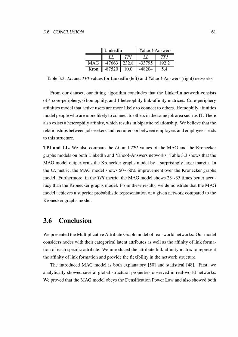
3.6. CONCLUSION 61
LinkedIn Yahoo!-Answers
LL TPI LL TPI
MAG -47663 232.8 -33795 192.2
Kron -87520 10.0 -48204 5.4
Table 3.3: LL and TPI values for LinkedIn (left) and Yahoo!-Answers (right) networks
From our dataset, our fitting algorithm concludes that the LinkedIn network consists
of 4 core-periphery, 6 homophily, and 1 heterophily link-affinity matrices. Core-periphery
affinities model that active users are more likely to connect to others. Homophily affinities
model people who are more likely to connect to others in the same job area such as IT. There
also exists a heterophily affinity, which results in bipartite relationship. We believe that the
relationships between job seekers and recruiters or between employers and employees leads
to this structure.
TPI and LL. We also compare the LL and TPI values of the MAG and the Kronecker
graphs models on both LinkedIn and Yahoo!-Answers networks. Table 3.3 shows that the
MAG model outperforms the Kronecker graphs model by a surprisingly large margin. In
the LL metric, the MAG model shows 50∼60% improvement over the Kronecker graphs
model. Furthermore, in the TPI metric, the MAG model shows 23∼35 times better accu-
racy than the Kronecker graphs model. From these results, we demonstrate that the MAG
model achieves a superior probabilistic representation of a given network compared to the
Kronecker graphs model.
3.6 Conclusion
We presented the Multiplicative Attribute Graph model of real-world networks. Our model
considers nodes with their categorical latent attributes as well as the affinity of link forma-
tion of each specific attribute. We introduced the attribute link-affinity matrix to represent
the affinity of link formation and provide the flexibility in the network structure.
The introduced MAG model is both explanatory [50] and statistical [48]. First, we
analytically showed several global structural properties observed in real-world networks.
We proved that the MAG model obeys the Densification Power Law and also showed both

62 CHAPTER 3. MODEL FOR NETWORK LINKS
the existence of unique giant connected component and a small diameter under the MAG
model. Furthermore, we mathematically analyzed that the MAG model gives rise to net-
works with either a log-normal or a power-law degree distribution.
Second, we developed MAGFIT, a scalable variational expectation maximization method
for parameter estimation of the MAG model. Empirical experiments on real-world net-
works showed that the MAG model reliably captures both global structural properties and
local linking patterns of given networks. Moreover, the MAG model can provide insights
into how different latent attributes shape the structure of networks.

Chapter 4
Model for Networks with Node Features
Network data, such as social networks of friends, citation networks of documents, and
hyper-linked networks of webpages, plays an increasingly important role in modern ma-
chine learning applications. Analyzing network data provides useful predictive models
for recommending new friends in social networks [4] or scientific papers in document net-
works [16,77]. As our model in the previous chapter accurately captured the global network
structure, research on networks has focused on modeling network link structure.
In many cases, node features can be observed along with network links, but node fea-
tures have been mostly ignored in traditional models for networks. For example, in social
networks users have profile information, and in document networks each node also con-
tains the text of the document that it represents. The models that only use network links
can find patterns of links between the users or between the documents, but cannot account
for the node features, profile or text.
Like network links, node features provide rich and complementary sources of informa-
tion, so they should be used simultaneously to uncover, understand and exploit the latent
structure in network data. Considering both sources of data – links and node features –
leads to more powerful models than models that consider only links. For example, given
a new node with a few of its links, traditional network models provide a predictive distri-
bution of other nodes to which the new one might be connected. In contrast, if a model
considers both links and node features, then we can predict links of a new node without
seeing any of the node’s existing links. For example, we can suggest a user’s friendships
63

64 CHAPTER 4. MODEL FOR NETWORKS WITH NODE FEATURES
based only on his or her profile information and recommend hyperlinks of a webpage based
only on its textual information. Moreover, given a new node and its links, our model also
provides a predictive distribution of node features. This model can be used to predict fea-
tures of a node given its links or even predict missing or hidden features of a node given
its links. For example, interests of a user or keywords of a webpage can be predicted us-
ing only the connections of the network. Such predictions are out of reach for traditional
network models.
To enjoy the power of using both network links and node features, we develop a Latent
Multi-group Membership Graph (LMMG) model of networks that extends the MAG model
by tying nodes into groups of shared node features and linking structure. To elaborate,
each node belongs to multiple latent groups, and the occurrence of each node feature is
determined by a generative model based on the group memberships of the given node.
Links of the network are then generated via link-affinity matrices as in the MAG model.
We derive efficient algorithms for model parameter estimation and prediction and study the
performance of LMMG on real-world social and document networks. We also investigate
predictive performance on three different tasks: node feature prediction, link prediction,
and supervised node classification. The LMMG provides significantly better performance
on all three tasks than natural alternatives and the current state of the art.
The rest of this chapter is organized as follows: Section 2 provides related work. Sec-
tion 3 presents our generative model, and its fitting algorithm follows in Section 4. Finally,
Section 5 shows experimental results on three kinds of prediction tasks and describes a case
study on a Facebook ego-network.
4.1 Related Work
Before describing our model, we begin by the survey of some related work.
Models of networks with node features. A line of research has studied the network model
considering node features. Because of plentiful work on text documents, there exist many
document/coauthorship network models that incorporate the topic from documents. For ex-
ample, the Pairwise Link-LDA model (PL-LDA) blends the Mixed-membership Stochastic

4.1. RELATED WORK 65
Blockmodel and the Latent Dirichlent Allocation into one framework with regard to doc-
ument network [77]. Another example includes the Relational Topic Model (RTM) which
defines the relationships between documents on top of LDA topic model [16]. However,
the node features of both models are limited to words which have the same distribution
according to the topic, whereas the node features in our model do not have such restriction.
Also in biology, there have been similar attempts to present a method for clustering
genes based on microarray expression data (node features) and a given gene network [92].
Historically, the above models have been however developed by smoothly turning focus
to networks from long-lived text analysis research with vector form of data. In contrast, the
Exponential Random Graph Model (ERGM) [103] and the Multiplicative Attribute Graphs
(MAG) model [50] have added a framework for node features on top of network model.
While ERGM pays more attention to the local network patterns, the MAG model considers
the global network structure, similarly to our approach, so that it holds most real-world
network properties such as small diameter [104]. However, the MAG model is difficult
to by itself determine proper combination of real-world node features associated with the
network structure. Our model resolves this issue by connecting the global network structure
to real-world node features via latent groups.
Collective classification. In addition to network models with node features, there have
been attempts to exploit the network dependencies as well as node features for the node
labeling task. Collective Classification is one of the methods to consider the network de-
pendencies under the supervised setting [90]. For example, based on the assumption of
homophily (more links between nodes with the same features), one can take the aggregate
information of neighbor nodes as one feature of supervised learning. However, the attention
has been paid more to the classification task than the generative model for node features
and network links. Moreover, this approach usually focuses only on the neighbors of a
given node due to the homophily assumption, while our model can capture more flexible
global network structure, including homophily (love of the same), heterophily (love of the
different), and core-periphery (love of the core).

66 CHAPTER 4. MODEL FOR NETWORKS WITH NODE FEATURES
Figure 4.1: Latent Multi-group Membership Graph model. A node belongs to multiple
latent groups at once. Based on group memberships features of a node are generated us-
ing a logistic model. Links are modeled via link-affinity matrices which allows for rich
interactions between members and non-members of groups.
4.2 Latent Multi-group Membership Graph
Our Latent Multi-group Membership Graph (LMMG) model is a model of a (directed or
undirected) network and its nodes, which have categorical features. It contains two impor-
tant components (See Figure 4.1).
First, the model assigns nodes to latent groups and allows nodes to belong to multiple
groups at once. In contrast to multinomial models of group membership [1, 16] where the
membership of a node is shared among the groups (the probability over group member-
ships of a node sums to 1), we model group memberships as a series of Bernoulli random
variables (φi in Figure 4.1), thereby indicating that nodes in our model can truly belong
to multiple groups. Thus, in contrast to multinomial topic models, in the LMMG model a
higher probability of node membership to one group does not necessarily lower the proba-
bility of membership to some other group.
Second, to model the links of the network, we associate each group k with a link-
affinity matrix (Θ in Figure 4.1) as in the previous chapter. Here each link-affinity matrix
represents a table of link affinities given that a pair of nodes belongs or does not belong

4.2. LATENT MULTI-GROUP MEMBERSHIP GRAPH 67
Figure 4.2: Plate model representation of the LMMG model.
to group k. Thus, depending on the combination of the memberships of nodes to group k,
an appropriate element of Θk is chosen. For example, the entry (0, 0) of Θk captures the
link-affinity when none of the nodes belongs to group k, while (1, 0) stores the link-affinity
when the first node belongs to the group (1) but the second does not (0). As we have shown
in the previous chapter, this allows for rich flexibility in modeling the links of the network
as well as for uncovering and understanding the latent structure of the network.
Next we formalize the LMMG model illustrated in Figure 4.2 and describe it in a gen-
erative way. Formally, each node i = 1, 2, · · · , N has a real-valued group membership
φik ∈ [0, 1] for each group k = 1, 2, · · · , K. The value φik represents the probability that
node i belongs to group k. Assuming the Beta distribution parameterized by αk1, αk2 as a
prior distribution of group membership φik, we model the latent group assignment zik for
each node as follows:
φik ∼ Beta(αk1, αk2)
zik ∼ Bernoulli(φik) for k = 1, 2, · · · , K . (4.1)
Since each group membership zik of a node is independent, a node can belong to multiple
groups simultaneously.
The group memberships of a node affect both the node’s features and the node’s links.
With respect to node features, we limit our focus to binary-valued features and use a logistic
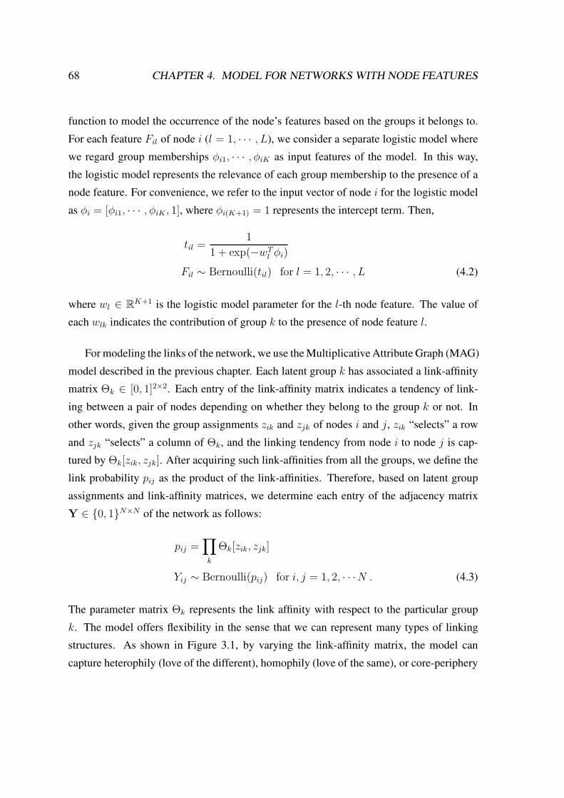
68 CHAPTER 4. MODEL FOR NETWORKS WITH NODE FEATURES
function to model the occurrence of the node’s features based on the groups it belongs to.
For each feature Fil of node i (l = 1, · · · , L), we consider a separate logistic model where
we regard group memberships φi1, · · · , φiK as input features of the model. In this way,
the logistic model represents the relevance of each group membership to the presence of a
node feature. For convenience, we refer to the input vector of node i for the logistic model
as φi = [φi1, · · · , φiK , 1], where φi(K+1) = 1 represents the intercept term. Then,
til =1
1 + exp(−wTl φi)
Fil ∼ Bernoulli(til) for l = 1, 2, · · · , L (4.2)
where wl ∈ RK+1 is the logistic model parameter for the l-th node feature. The value of
each wlk indicates the contribution of group k to the presence of node feature l.
For modeling the links of the network, we use the Multiplicative Attribute Graph (MAG)
model described in the previous chapter. Each latent group k has associated a link-affinity
matrix Θk ∈ [0, 1]2×2. Each entry of the link-affinity matrix indicates a tendency of link-
ing between a pair of nodes depending on whether they belong to the group k or not. In
other words, given the group assignments zik and zjk of nodes i and j, zik “selects” a row
and zjk “selects” a column of Θk, and the linking tendency from node i to node j is cap-
tured by Θk[zik, zjk]. After acquiring such link-affinities from all the groups, we define the
link probability pij as the product of the link-affinities. Therefore, based on latent group
assignments and link-affinity matrices, we determine each entry of the adjacency matrix
Y ∈ 0, 1N×N of the network as follows:
pij =∏
k
Θk[zik, zjk]
Yij ∼ Bernoulli(pij) for i, j = 1, 2, · · ·N . (4.3)
The parameter matrix Θk represents the link affinity with respect to the particular group
k. The model offers flexibility in the sense that we can represent many types of linking
structures. As shown in Figure 3.1, by varying the link-affinity matrix, the model can
capture heterophily (love of the different), homophily (love of the same), or core-periphery

4.3. INFERENCE ALGORITHM 69
structure. In this way the affinity matrix allows us to discover the effects of node features
on links of the network.
The node features and the links of the network are connected via group memberships
φi. For instance, suppose that wlk is large for some feature l and group k. Then, as the node
i belongs to group k with high probability (φik is close to 1), the feature l of node i, Fil,
is more likely to be 1 than 0. By modeling group memberships using multiple Bernoulli
random variables (instead of using multinomial distribution [1, 16]), we achieve greater
modeling flexibility, which allows for making predictions about links given features, and
features given links. In Section 4.4, we empirically demonstrate that the LMMG model
outperforms traditional models on these tasks.
Moreover, if we divide the nodes of the network into two sets depending on the mem-
bership to group k, then we can discover how members of group k link to other members
as well as to non-members of group k, based on the structure of Θk. For example, when Θk
has large values on its diagonal entries, members or non-members are likely to link among
themselves, while there is low affinity for links between members and non-members. Θk
with large off-diagonal entry values captures exactly the opposite behavior, where links are
most likely between members and non-members. The core-periphery structure can also be
captured when nodes that share group memberships (the “core”) are most likely to link,
while nodes in the periphery are least likely to link among themselves.
4.3 Inference Algorithm
We now turn our attention to the LMMG model estimation. Given a set of binary node fea-
tures F and the adjacency matrix of a network Y, we aim to find node group memberships
Φ, parameters W of node feature model, and link-affinity matrices Θ.
4.3.1 Problem formulation
When the node features F = Fil : i = 1, · · · , N, l = 1, · · · , L and the adjacency
matrix Y ∈ 0, 1N×N are given, we aim to find the latent group memberships Φ =
φik : i = 1, · · · , N, k = 1, · · · , K, the logistic model parameters W = wlk : l =

70 CHAPTER 4. MODEL FOR NETWORKS WITH NODE FEATURES
1, · · · , L, k = 1, · · · , K+1, and the link-affinity matrices Θ = Θk : k = 1, · · ·K. We
apply the maximum likelihood estimation, which finds the optimal values of Φ, W, and Θ
so that they maximize the likelihood P (F,Y,Φ|W,Θ, α), where α = (αk1, αk2) : k =
1, · · · , K represents hyper parameters for the Beta prior distributions. In the end, we aim
to solve
maxΦ,W,Θ
logP (F,Y,Φ|W,Θ, α) . (4.4)
Now we compute the objective function in the above optimization problem. Since the
LMMG independently generates F and Y given latent group memberships Φ, we decom-
pose the log-likelihood logP (F,Y,Φ|W,Θ, α) as follows:
logP (F,Y,Φ|W,Θ, α) = logP (F|Φ,W) + logP (Y|Φ,Θ) + logP (Φ|α) . (4.5)
Hence, to compute logP (F,Y,Φ|W,Θ, α), we separately calculate each term of Equa-
tion (4.5). We obtain logP (Φ|α) and logP (F|Φ,W) from Equations (4.1) and (4.2):
logP (Φ|α) =∑
i,k
(αk1 − 1) logφik +∑
i,k
(αk2 − 1) log(1− φik)
logP (F|Φ,W) =∑
i,l
Fil log til + (1− Fil) log(1− til)
where til are defined in Equation (4.2).
With regard to the second term in Equation (4.5),
logP (Y|Φ,Θ) = log∑
Z
P (Y|Z,Φ,Θ)P (Z|Φ,Θ) (4.6)
for Z = zik : i = 1, · · · , N, k = 1, · · · , K. Note that Y is independent of Φ given
Z. To exactly calculate logP (Y|Φ,Θ), we sum P (Y|Z,Θ)P (Z|Φ) over every instance
of Z given Θ and Φ. However, this requires the sum over 2NK instances. As this exact
computation is infeasible, we approximate logP (Y|Φ,Θ) using its lower bound obtained
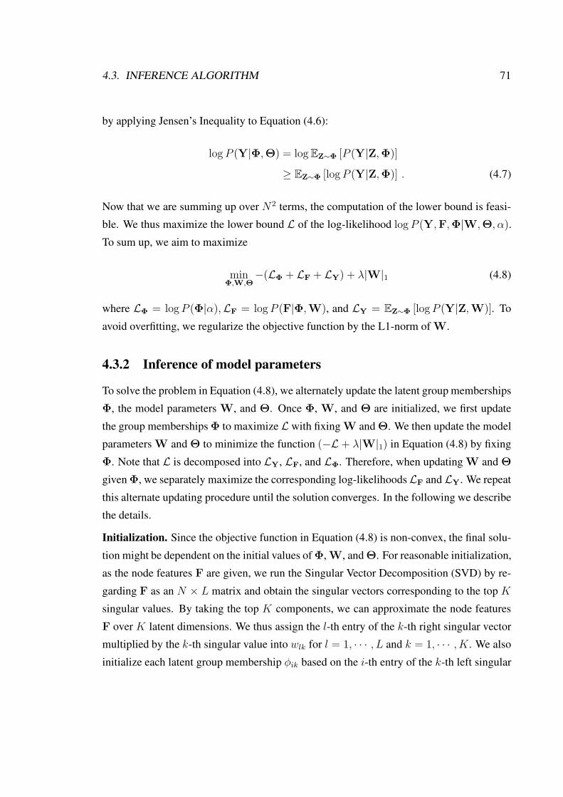
4.3. INFERENCE ALGORITHM 71
by applying Jensen’s Inequality to Equation (4.6):
logP (Y|Φ,Θ) = logEZ∼Φ [P (Y|Z,Φ)]
≥ EZ∼Φ [logP (Y|Z,Φ)] . (4.7)
Now that we are summing up over N2 terms, the computation of the lower bound is feasi-
ble. We thus maximize the lower bound L of the log-likelihood logP (Y,F,Φ|W,Θ, α).
To sum up, we aim to maximize
minΦ,W,Θ
−(LΦ + LF + LY) + λ|W|1 (4.8)
where LΦ = logP (Φ|α),LF = logP (F|Φ,W), and LY = EZ∼Φ [logP (Y|Z,W)]. To
avoid overfitting, we regularize the objective function by the L1-norm of W.
4.3.2 Inference of model parameters
To solve the problem in Equation (4.8), we alternately update the latent group memberships
Φ, the model parameters W, and Θ. Once Φ, W, and Θ are initialized, we first update
the group memberships Φ to maximize L with fixing W and Θ. We then update the model
parameters W and Θ to minimize the function (−L + λ|W|1) in Equation (4.8) by fixing
Φ. Note that L is decomposed into LY, LF, and LΦ. Therefore, when updating W and Θ
given Φ, we separately maximize the corresponding log-likelihoodsLF and LY. We repeat
this alternate updating procedure until the solution converges. In the following we describe
the details.
Initialization. Since the objective function in Equation (4.8) is non-convex, the final solu-
tion might be dependent on the initial values of Φ, W, and Θ. For reasonable initialization,
as the node features F are given, we run the Singular Vector Decomposition (SVD) by re-
garding F as an N × L matrix and obtain the singular vectors corresponding to the top K
singular values. By taking the top K components, we can approximate the node features
F over K latent dimensions. We thus assign the l-th entry of the k-th right singular vector
multiplied by the k-th singular value into wlk for l = 1, · · · , L and k = 1, · · · , K. We also
initialize each latent group membership φik based on the i-th entry of the k-th left singular

72 CHAPTER 4. MODEL FOR NETWORKS WITH NODE FEATURES
vectors. This approximation can in particular provide good enough initial values when the
top K singular values dominate the others. In order to obtain sparse model parameters W,
we reassign 0 to wlk of small absolute value such that |wlk| < λ.
Finally, to initialize the link-affinity matrices Θ, we introduce the following way. When
initializing the k-th link-affinity matrix Θk, we assume that the group other than the k-th
group has nothing to do with network structure, i.e. every entry in the other link-affinity
matrices has the equal value. Then, we compute the ratio between entries Θk[x1, x2] for
x1, x2 ∈ 0, 1 as follows:
Θk[x1, x2] ∝∑
i,j:Yij=1
EZ∼ΦP [zik = x1, zik = x2] .
As the latent group memberships Φ are initialized above and zik and zjk are independent
of each other, we are able to compute the ratio between entries of Θk. After computing the
ratio between entries for each link-affinity matrix, we adjust the scale of the link-affinity
matrices so that the expected number of edges in the MAG model is equal to the number of
edges in the given network, i.e.∑
i,j pij =∑
i,j Yij .
Update of latent group memberships Φ. Now we focus on updating the latent group
memberships Φ given the model parameters W and Θ. We use the coordinate ascent
algorithm which updates each membership φik by fixing the others so to maximize the
lower bound L. By computing the derivatives of LΦ, LF, and LY we apply the gradient
method to update each φik:
∂LΦ
∂φik=
αk1 − 1
φik− αk2 − 1
1− φik
∂LF
∂φik=∑
l
(Fil − til)wlk
∂LY
∂φik= EZ∼Φ
∑
j:Yij=1
∂ log pij∂φik
+∑
j:Yij=0
∂ log(1− pij)
∂φik+∑
j:Yji=1
∂ log pji∂φik
+∑
j:Yji=0
∂ log(1− pji)
∂φik
(4.9)
where Fil is either 0 or 1, and til and pij is respectively defined in Equation (4.2) and (4.3).
We ignore the term corresponding to i = j in this computation.

4.3. INFERENCE ALGORITHM 73
To complete this computation, we need to calculate∂EZ∼Φ log pij
∂φikand
∂EZ∼Φ log(1−pij)
∂φik. We
then apply the same technique to the computation of∂EZ∼Φ log pji
∂φikand
∂EZ∼Φ log(1−pji)
∂φik.
We begin by computing the derivative of expected log-likelihood for each link, EZ∼Φ log pij .
When all the latent group memberships except for φik are fixed, we can derive∂EZ∼Φ log pij
∂φik
from definition of pij in Equation (4.3) as follows:
∂EZ∼Φ log pij∂φik
=∂
∂φikEZ∼Φ
[
∑
k′
log Θk′[zik′, zjk′]
]
=∑
k′
[
∂
∂φikEZ∼Φ logΘk′[zik′ , zjk′]
]
. (4.10)
Here we use the following property to compute the above formula. Since zik is an indepen-
dent Bernoulli random variable with probability φik, for any function f : 0, 12 → R,
EZ∼Φf(zik, zjk) = φikφjkf(1, 1) + φik(1− φjk)f(1, 0)
+ (1− φik)φjkf(0, 1) + (1− φik)(1− φjk)f(0, 0) . (4.11)
Hence, by applying Equation (4.11) to (4.10), we obtain
∂EZ∼Φ log pij∂φik
=∂
∂φik
EZ∼Φ logΘk[zik, zjk]
= (φjk log Θk [1, 1] + (1− φjk) log Θk [1, 0])
− (φjk log Θk [0, 1] + (1− φjk) log Θk [0, 0]) . (4.12)
Next, we compute the derivative of expected log-likelihood for unlinked node pairs,
i.e. EZ∼Φ log(1−pij). Here we approximate the computation using the Taylor’s expansion,
log(1− x) ≈ −x− 0.5x2 for small x:
∂EZ∼Φ log(1− pij)
∂φik≈ −∂EZ∼Φpij
∂φik− 0.5
∂EZ∼Φp2ij
∂φik.

74 CHAPTER 4. MODEL FOR NETWORKS WITH NODE FEATURES
To compute∂EZ∼Φpij
∂φik,
∂EZ∼Φpij∂φik
=∂
∂φikEZ∼Φ
∏
k′
Θk′[zik′ , zjk′]
=∂
∂φikEZ∼ΦΘk[zik, zjk]
∏
k′ 6=k
Θk′[zik′, zjk′]
=∏
k′ 6=k
EZ∼ΦΘk′[zik′ , zjk′]∂
∂φik
EZ∼ΦΘk[zik, zjk] .
By Equation (4.11), each EZ∼ΦΘk[zik, zjk] and its derivative can be obtained. Similarly,
we can calculate∂EZ∼Φp2ij
∂φik, so we complete the computation of
∂EZ∼Φ log(1−pij)
∂φik. As we attain
∂EZ∼Φ log pij∂φij
and∂EZ∼Φ log(1−pij)
∂φij, we eventually calculate ∂LY
∂φik. Hence, by adding up ∂LΦ
∂φik,
∂LF
∂φik, and ∂LY
∂φik, we complete computing the derivative of the lower bound of log-likelihood
∂L∂φik
and update each latent group membership φik using the gradient method:
∂L∂φik
=∂LY
∂φik
+∂LF
∂φik
+∂LY
∂φik
φnewik = φold
ik + γΦ
(
∂LY
∂φik+
∂LF
∂φik+
∂LY
∂φik
)
for a given learning rate γΦ. By updating each φik in turn by fixing the others, we then find
the optimal latent group memberships Φ given the model parameters W and Θ.
Update of node feature model parameters W. Now we update the parameters W of
node feature model while keeping latent group memberships Φ fixed. Note that given the
group memberships Φ the node feature model and the network model are independent of
each other. Therefore, finding parameters W is equivalent to running the L1-regularized
logistic regression given input Φ and output F data as we penalize the objective function
in Equation (4.8) on the L1 value of model parameters W. We basically use the gradient

4.3. INFERENCE ALGORITHM 75
method to update W but make it sparse by applying the technique similar to LASSO:
∂LF
∂wlk
=∑
i
(Fil − til)φik
wnewlk = wold
lk + γF∂LF
∂wlk
− λ(k)Sign(wlk) (4.13)
if woldlk 6= 0 or | ∂LF
∂wlk| > λ(k) where λ(k) = λ for k = 1, · · · , K and λ(K + 1) = 0 (i.e.,
we do not regularize on the intercepts). γF is a constant learning rate. Furthermore, if wlk
crosses 0 while being updated, we assign 0 to wlk, same as in LASSO. By this procedure,
we can update the node feature model parameters W to maximize the lower bound of
log-likelihood L as well as to maintain the small number of relevant groups for each node
feature.
Update of network model parameters Θ. Next we focus on updating network model pa-
rameters, Θ, when the latent group memberships Φ are fixed. Again, note that the network
model is independent of the node feature model given the latent group memberships Φ, so
we do not need to consider LΦ or LF. We thus update Θ to maximize LY given Φ using
the gradient method.
As we previously did in computing ∂LY
∂φikby separating edge and non-edge terms, we
compute each ∂LY
∂Θk[x1,x2]for k = 1, · · · , K and x1, x2 ∈ 0, 1. To describe mathematically,
∂LY
∂Θk[x1, x2]=∑
Yij=1
∂EZ∼Φ log pij∂Θk[x1, x2]
+∑
Yij=0
∂EZ∼Φ log(1− pij)
∂Θk[x1, x2]. (4.14)
Now we compute each term in the above calculation by the definition of pij . First, we
compute the former term by using Equation (4.11). For instance,
∂LY
∂Θk[0, 1]= (1− φik)φjk
∂ logΘk[0, 1]
∂Θk[0, 1]=
(1− φik)φjk
Θk[0, 1].
Hence, we can properly compute Equation (4.14) depending on the values of x1 and x2.

76 CHAPTER 4. MODEL FOR NETWORKS WITH NODE FEATURES
Second, we use the same Taylor’s expansion technique for the latter term in Equa-
tion (4.14) as follows:
∂EZ∼Φ log(1− pij)
∂Θk[x1, x2]≈ ∂
∂Θk[x1, x2]EZ∼Φ
(
−pij − 0.5p2ij)
.
Similarly toEZ∼Φpij
∂φik,
EZ∼Φpij∂Θk[x1,x2]
is computed by
∏
k′ 6=k
EZ∼ΦΘk′[zik′, zjk′]∂
∂Θk[x1, x2]EZ∼ΦΘk[zik, zjk]
where each term is obtained by Equation (4.11). Similarly, we computeEZ∼Φp2ij∂Θk[x1,x2]
so that
we can obtain ∂LY
∂Θk[x1,x2].
In consequence, we can compute the gradient for each Θk and update it to maximize
the lower bound LY by the gradient method:
∇ΘkLY ≈ ∇Θk
EZ∼Φ
∑
Yij=1
log pij +∑
Yij=0
log(1− pij)
Θnewk = Θold
k + γY∇ΘkLY
for a constant learning rate γY.
Prediction. With a fitted model, our ultimate goal is to make predictions about new data. In
real-world application, the node features are often missing. Our approach is able to handle
such missing node features by fitting the LMMG model only to the observed features.
In other words, when we update the latent group memberships Φ or the feature model
parameters W by the gradient method from Equation (4.9) and (4.13), we only average the
terms corresponding to the observed data. For example, when there is missing feature data,
Equation (4.9) can be converted into:
∂LF
∂φik=
∑
l:Fil∈O(Fil − til)wlk
∑
l:Fil∈O1
(4.15)
for the observed data O.

4.4. EXPERIMENTS 77
Similarly, for link prediction we modify the model estimation method as follows. While
updating the node feature model parameters W based on the features of all the nodes
including a new node, we estimate the network model parameters Θ only on the observed
network by holding out the new node. This way, the observed features naturally update
the latent group memberships of a new node. We then predict the missing node features or
network links by using the estimated group memberships and model parameters.
Selection of the Number of Groups K. Another issue in fitting the LMMG model to
the given network and node feature data is to determine the number of latent groups, K.
We can find the insight about the value of K from the MAG model. It has been already
proved that, in order for the MAG model to reasonably represent the real-world network,
the value of K should be in the order of logN where N represents the number of nodes in
the network [50]. Since in the LMMG model the network links are modeled similarly to
the MAG model, the same argument on the number of groups K still holds.
However, the above argument cannot determine the specific value of K. To select one
value of K, we use the cross-validation method as follows. For instance, suppose that
we aim to predict all the features of a node where its links to the other nodes are fully
observed (Task 1 in Section 4.4). While holding out the test node, we can set up the
same prediction task in a way that we select one at random from the other nodes (training
nodes) and regard it as the validation test node. We then perform the missing node feature
prediction on this validation node and obtain the log-likelihood result. By running this
procedure with varying the validation test node, we can attain the average log-likelihood
on the missing node features given the specific value of K (i.e. N-fold cross-validation).
Finally, we compare the average log-likelihood values according the value of K and pick
up the best one to maximize the log-likelihood. This method can be done by the other
prediction tasks, missing link prediction and supervised node classification.
4.4 Experiments
In the previous section, we described the algorithm which fits the LMMG model to the
real-world data containing a network and the corresponding node features. To evaluate our

78 CHAPTER 4. MODEL FOR NETWORKS WITH NODE FEATURES
proposed model and the fitting algorithm, here we perform various prediction tasks: miss-
ing node feature prediction, missing link prediction, and supervised node classification. In
all tasks our model outperforms natural baselines. Furthermore, we qualitatively analyze
the relationships between the node features and the network structure by a case study of a
Facebook ego-network and show how the LMMG model identifies useful and interpretable
latent structures.
Datasets. For our experiments, we used the following datasets containing networks and
node features.
• AddHealth (AH): School friendship network (458 nodes, 2,130 edges) with 35 school-
related node features such as GPA, courses taken, and placement [6].
• Egonet (EGO): Facebook ego-network of a particular user (227 nodes, 6,348 edges)
and 14 binary features (e.g. same high school, same age, and sports club), manually
assigned to each friend by the ‘ego’ user.
• Facebook100 (FB): Facebook network of Caltech (769 nodes, 33,312 edges) and 24
university-related node features like major, gender, and dormitory [98].
• WebKB (WKB): Hyperlinks between computer science webpages of Cornell Uni-
versity in the WebKB dataset (195 nodes, 304 edges). We use occurrences of 993
words as binary features [20].
We binarized discrete valued features (e.g. school year) based on whether the feature value
is greater than the median value. For the non-binary categorical features (e.g. major), we
used an indicator variable for each possible feature value. Some of these datasets are avail-
able at http://snap.stanford.edu.
Predictive tasks. We investigate the predictive performance of the LMMG model based
on three different tasks. We visualize them in Figure 4.3. Note that the column represents
either features or nodes depending on the type of the task. For each matrix, given 0/1
values in the white area, we predict the values of the entries with question marks. First,
assuming that all node features of a given node are completely missing, we predict all the
features based on the links of the node (Figure 4.3(a)). Second, when all the links of a

4.4. EXPERIMENTS 79
(a) Missing feature prediction (b) Missing link prediction (c) Supervised node classification
Figure 4.3: Three link and feature based predictive tasks.
given node are missing, we predict the missing links by using the node feature information
(Figure 4.3(b)). Last, we assume only few features of a node are missing and perform
supervised classification of a specific node feature given all the other node features and the
network (Figure 4.3(c)).
Baseline models. Next we introduce natural baseline as well as the state-of-the-art meth-
ods. First, for the most basic baseline, when predicting some missing value (node feature
or link) of a given node, we average the corresponding values of all the other nodes and
regard it as the probability of value 1. We refer to this algorithm as AVG. Second, as
we can view each of the three prediction tasks as the classification task, we use Collec-
tive Classification (CC) algorithms that exploit both node features and network dependen-
cies [90]. For the local classifier of CC algorithms, we use Naive-Bayes (CC-N) as well
as logistic regression (CC-L). We also compare the LMMG model to the state of the art,
the Relational Topic Model (RTM) [16]. For the Relational topic model, we use the lda-R
package (http://cran.r-project.org/web/packages/lda/index.html).
Task 1: Predicting missing node features. First, we examine the task of predicting miss-
ing features of a node where features of other nodes and all the links are observed. We
randomly select a node and remove all the feature values of that node and then try to re-
cover them. We quantify the performance by using the log-likelihood of the true feature
values over the estimated distributions as well as the predictive accuracy (the probability of
correctly predicting the missing features) of each method.

80 CHAPTER 4. MODEL FOR NETWORKS WITH NODE FEATURES
LL
AVG CC-N CC-L RTM LMMG
AH -23.0 -17.6 -16.8 -63.4 -15.6
EGO -5.4 -6.6 -5.1 -9.9 -3.7
FB -8.7 -11.6 -8.9 -19.0 -7.4
WKB -179.3 -186.8 -179.2 -336.8 -173.6
ACC
AVG CC-N CC-L RTM LMMG
AH 0.53 0.61 0.56 0.59 0.64
EGO 0.79 0.81 0.78 0.74 0.86
FB 0.77 0.76 0.75 0.77 0.80
WKB 0.88 0.88 0.89 0.88 0.90
Table 4.1: Prediction of missing node features: The LMMG performs the best in terms of
the log-likelihood as well as the classification accuracy on the held-out data.
Table 4.1 shows the results of the experiments by measuring the average of log-likelihood
(LL) and prediction accuracy (ACC) for each algorithm and each dataset. We notice that the
LMMG model exhibits the best performance in the log-likelihood for all datasets. While
CC-L in general performs the second best, our model outperforms it by up to 23%. The
performance gain over the other models in terms of accuracy seems smaller when com-
pared to the log-likelihood. However, the LMMG model still predicts the missing node
features with the highest accuracy on all the datasets.
In particular, the LMMG model exhibits the most improvement in node feature predic-
tion on the ego-network dataset (30% in LL and 7% in ACC) over the next best method.
Here node features are derived by manually labeling community memberships of each per-
son in the ego-network. Thus, a group of people in the network intrinsically share some
node feature value (community membership). In this sense, the node features and the links
in the ego-network are directly related to each other and our model successfully exploits
this relationship to predict missing node features.
Task 2: Predicting missing links. Second, we also consider the task of predicting missing
links of a specific node while the features of the node are given. Similarly to the previous
task, we select a node at random, but here we remove all its links while observing its fea-
tures. We then aim to recover the missing links. For evaluation, we use the log-likelihood

4.4. EXPERIMENTS 81
LL
AVG CC-N CC-L RTM LMMG
AH -40.2 -57.2 -38.9 -100.6 -36.1
EGO -142.7 -134.3 -157.6 -149.9 -125.9
FB -320.8 -330.7 -345.6 -359.1 -328.3
WKB -54.2 -185.5 -39.6 -25.8 -13.7
AUC
AVG CC-N CC-L RTM LMMG
AH 0.51 0.69 0.39 0.56 0.72
EGO 0.61 0.89 0.55 0.49 0.89
FB 0.73 0.70 0.57 0.46 0.73
WKB 0.70 0.86 0.55 0.50 0.89
Table 4.2: Prediction of missing links of a node. The LMMG model performs best in all
but one case.
(LL) of missing links as well as the area under the ROC curve (AUC) of missing link
prediction.
We give the experimental results for each dataset in Table 4.2. Again, the LMMG out-
performs the baseline models in the log-likelihood except for the Facebook100 data. Inter-
estingly, while RTM was relatively competitive when predicting missing features, it tends
to fail predicting missing links, which implies that the flexibility of link-affinity matrices is
needed for accurate modeling of the links.
We observe that Collective Classification methods look competitive in some perfor-
mance metrics and datasets. For example, CC-N gives good results in terms of classification
accuracy, and CC-L performs well in terms of the log-likelihood. As CC-N is a discrim-
inative model, it does not perform well in missing link probability estimation. However,
the LMMG model is a generative model that produces a joint probability of node features
and network links, so it is also very good at estimating missing links. Hence, in overall, the
LMMG model exploits the relationship between the network structure and node features to
predict missing links.
Task 3: Supervised node classification. Finally, we examine the performance on the
supervised classification task. In many cases, we aim to classify entities (nodes) based on
their feature values under the supervised setting. Here the relationships (links) between the
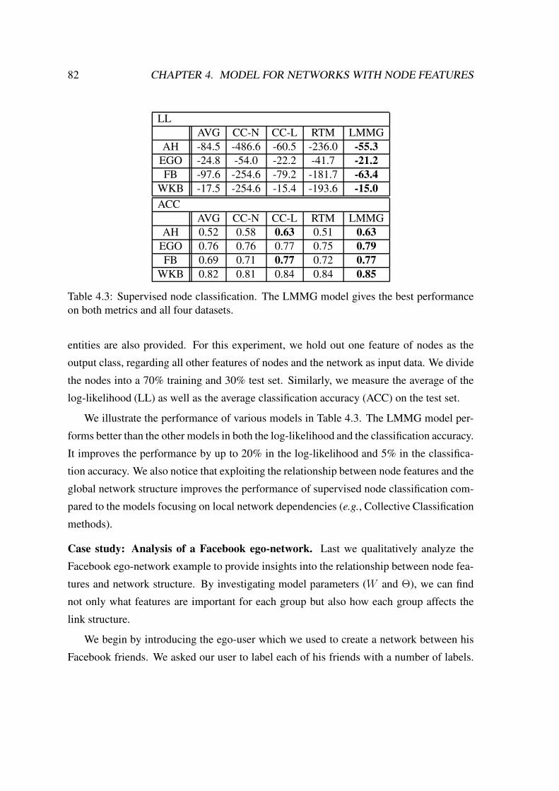
82 CHAPTER 4. MODEL FOR NETWORKS WITH NODE FEATURES
LL
AVG CC-N CC-L RTM LMMG
AH -84.5 -486.6 -60.5 -236.0 -55.3
EGO -24.8 -54.0 -22.2 -41.7 -21.2
FB -97.6 -254.6 -79.2 -181.7 -63.4
WKB -17.5 -254.6 -15.4 -193.6 -15.0
ACC
AVG CC-N CC-L RTM LMMG
AH 0.52 0.58 0.63 0.51 0.63
EGO 0.76 0.76 0.77 0.75 0.79
FB 0.69 0.71 0.77 0.72 0.77
WKB 0.82 0.81 0.84 0.84 0.85
Table 4.3: Supervised node classification. The LMMG model gives the best performance
on both metrics and all four datasets.
entities are also provided. For this experiment, we hold out one feature of nodes as the
output class, regarding all other features of nodes and the network as input data. We divide
the nodes into a 70% training and 30% test set. Similarly, we measure the average of the
log-likelihood (LL) as well as the average classification accuracy (ACC) on the test set.
We illustrate the performance of various models in Table 4.3. The LMMG model per-
forms better than the other models in both the log-likelihood and the classification accuracy.
It improves the performance by up to 20% in the log-likelihood and 5% in the classifica-
tion accuracy. We also notice that exploiting the relationship between node features and the
global network structure improves the performance of supervised node classification com-
pared to the models focusing on local network dependencies (e.g., Collective Classification
methods).
Case study: Analysis of a Facebook ego-network. Last we qualitatively analyze the
Facebook ego-network example to provide insights into the relationship between node fea-
tures and network structure. By investigating model parameters (W and Θ), we can find
not only what features are important for each group but also how each group affects the
link structure.
We begin by introducing the ego-user which we used to create a network between his
Facebook friends. We asked our user to label each of his friends with a number of labels.

4.4. EXPERIMENTS 83
He chose to use 14 different labels. They correspond to his high school (HS), undergradu-
ate university (UNIVERSITY), math olympiad camp (CAMP), computer programming club
(KPROG) and work place (KCOMP) friends. The user also assigned labels to identify
friends from his graduate program (CS) and university (ST), basketball (BASKETBALL)
and squash (SQUASH) clubs, as well as travel mates (TRAVEL), summer internship buddies
(INTERN), family (FAMILY) and age group (AGE). We fit the LMMG model to the ego-
network and each friend’s labels, and obtained the model parameters W and Θ. We set the
number of latent groups to 5 since the previous prediction tasks worked well when K = 5.
In Table 4.4, for each of 5 latent groups, we represent the top 3 features with the largest
absolute value of model parameter |wlk| and the corresponding link-affinity matrices Θk.
We begin by investigating the first group. The top three labels the most correlated to
the first group are ST, AGE, and INTERN. However, notice that INTERN is negatively
correlated. This means that latent group 1 contains students from the same graduate school
and age, but not people with whom our user worked together at the summer internship (even
though they may be of the same school/age). We also note that Θ1 exhibits homophily
structure. From this we learn that summer interns, who met our Facebook user neither
because of shared graduate school nor because of age, form a group within which people
are densely connected. On the other hand, people of the same age at the same university
also exhibit homophily, but are less densely connected with each other. Such variation in
link density that depends on the group memberships agrees with our intuition. Those who
worked at the same company actively interact with each other so almost everyone is linked
in Facebook. However, as the group of people of the same university or age group is large
and each pair of people in that group does not necessarily know each other, the link affinity
in this group is naturally smaller than in the intern’s group.
Similarly, groups 2 and 3 form the two sports groups (BASKETBALL, SQUASH). People
are connected densely within each of the groups, but less connected to the outside of the
groups. Furthermore, we notice that those who graduated from the same high school (HS)
as well as the same undergraduate school (UNIVERSITY) form another community but the
membership to high school is more important than to the undergraduate university (8.7 vs.
2.3).

84 CHAPTER 4. MODEL FOR NETWORKS WITH NODE FEATURES
Group Top 1 Top 2 Top 3 Link-affinity matrix
1 ST (9.0) AGE (4.5) INTERN (-3.7) [0.67 0.08; 0.08 0.17]
2 HS (-8.7) UNIVERSITY (-2.3) BASKETBALL (2.2) [0.26 0.18; 0.18 0.38]
3 UNIVERSITY (-7.1) KORST (-2.6) SQUASH (2.2) [0.22 0.23; 0.23 0.32]
4 CS (7.3) FAMILY (7.0) CAMP (6.9) [0.25 0.24; 0.24 0.27]
5 KCOMP (5.2) KORST (4.4) INTERN (-3.8) [0.29 0.22; 0.22 0.27]
Table 4.4: Logistic model parameter values of top 3 features and the link-affinity matrix
associated with each group in the ego-network.
Last, for groups 4 and 5, we note that the corresponding link-affinity matrices are nearly
flat (i.e. values are nearly uniform). This implies that groups 4 and 5 are related to general
node features. In this sense, we hypothesize that features like CS, family, math camp, and
the company, have relatively little effect on the network structure.
4.5 Conclusion
The LMMG model builds on previous research in machine learning and network analy-
sis. Many models have been developed to explain network link structure [1, 41, 47, 59] and
extensions that incorporate node features have also been proposed [30, 48, 96]. However,
many of these models do not consider latent groups and thus cannot provide the bene-
fits of dimensionality reduction or produce interpretable clusters useful for understanding
network community structure.
The LMMG model provides meaningful clustering of nodes and their features in the
network. Network models of similar flavor have been proposed in the past [1, 41, 47], and
some even incorporate node features [16, 75, 77]. However, such models have been mainly
developed for document networks where they assume multinomial topic distributions for
each word in the document. We extend this by learning a logistic model of occurrence of
each feature based on node group memberships. We highlight this difference to previous
models. For topic memberships, previous models use multinomial distributions, where a
node has a mass of 1 to split among various topics. In contrast, under the LMMG a node
can belong to multiple topics at once without any constraint.

4.5. CONCLUSION 85
While previous work tends to explore only the network or only the features, the LMMG
model jointly models both so that it can make predictions of one given the other. The
LMMG models the interaction between links and group memberships through link-affinity
matrices, which provide great flexibility and interpretability of obtained groups and inter-
actions.
The LMMG model is a new probabilistic model of links and nodes in networks. It can
be used for link prediction, node feature prediction and supervised node classification. We
have demonstrated qualitatively and quantitatively that the LMMG model proves useful for
analyzing network data. The LMMG model significantly improves on previous models,
integrating both node-specific information and link structure to give better predictions.

86 CHAPTER 4. MODEL FOR NETWORKS WITH NODE FEATURES

Chapter 5
Model for Dynamic Networks
Chapter 3 presented a statistical analysis of social networks and other relational data, which
is becoming an important problem as the scope and availability of network data increases.
Network data – such as the friendships in a social network – is often dynamic in the sense
that relations between entities rise and decay over time. A fundamental problem in the
analysis of such dynamic network data is to extract a summary of the common structure
and the dynamics of the underlying relations between entities. Accurate models of the
structure and dynamics of network data have many applications. They allow us to predict
missing relationships [67, 75, 80, 86], recommend potential new relationships [4], identify
clusters and groups of nodes [1,107], forecast future links [27,36,39,87], and even predict
group growth and longevity [45].
Here we present a new approach to modeling network dynamics by considering time-
evolving interactions between groups of nodes as well as the arrival and departure dynamics
of individual nodes to these groups. We develop a dynamic network model, the Dynamic
Multi-group Membership Graph (DMMG) Model, which identifies the birth and death of
individual groups as well as the dynamics of node joining and leaving groups in order to
explain changes in the underlying network linking structure. Our nonparametric model
considers an infinite number of latent groups, in which each node can belong to multiple
groups simultaneously. We capture the evolution of individual node group memberships via
a Factorial Hidden Markov model. However, in contrast to recent works on dynamic net-
work modeling, we explicitly model the birth and death dynamics of individual groups by
87

88 CHAPTER 5. MODEL FOR DYNAMIC NETWORKS
using a distance-dependent Indian Buffet Process [29]. Under our model, only active/alive
groups influence the links between nodes in a network at a given time. We use a variant
of the MAG model presented in Chapter 3 to represent link structure depending on group
memberships of each node. In this way, we not only model relations between the mem-
bers of the same group but also account for links between members and non-members.
By explicitly modeling group lifespan and group connectivity structure, we achieve greater
modeling flexibility, which leads to improved performance on link prediction and network
forecasting tasks as well as to increased interpretability of obtained results.
The rest of this chapter is organized as follows: Section 5.1 provides the background
and related work. Section 5.2 presents our generative model and motivates its parametriza-
tion, and model inference procedure is presented in Section 5.3. Finally, in Section 5.4 we
provide experimental results as well as analysis of the social network from a movie, The
Lord of the Rings.
5.1 Related Work
Classically, non-Bayesian approaches such as exponential random graph models [38, 93]
have been used to study dynamic networks. On the other hand, in the Bayesian approaches
to dynamic network analysis latent variable models have been most widely used. These
approaches differ by the structure of the latent space that they assume. For example, Eu-
clidean space models [41, 87] place nodes in a low dimensional Euclidean space and the
network evolution is then modeled as a regression problem of node’s future latent loca-
tion. In contrast, our model uses HMMs, where latent variables stochastically depend on
the state at the previous time step. Related to our work are dynamic mixed-membership
models where a node is probabilistically allocated to a set of latent features. Examples of
this model include the dynamic mixed-membership block model [28, 40] and the dynamic
infinite relational model [44]. However, the critical difference here is that our model uses
multi-memberships where node’s membership to one group does not limit its membership
to other groups. Probably most related to our work here are DRIFT [27] and LFP [39] mod-
els. Both of these models consider Markov switching of latent multi-group memberships

5.2. NONPARAMETRIC DYNAMIC MULTI-GROUP MEMBERSHIP GRAPH 89
over time. DRIFT uses the infinite factorial HMM [100], while LFP adds “social propaga-
tion” to the Markov processes so that network links of each node at a given time directly
influence group memberships of the corresponding node at the next time. Compared to
these models, we uniquely incorporate the model of group birth and death and present a
novel and powerful linking function.
5.2 Nonparametric Dynamic Multi-group Membership Graph
First, we describe general components of modern dynamic network models [27,28,39,44].
In the next section we will then describe our own model and point out the differences to the
previous work.
Dynamic networks are generally conceptualized as discrete time series of network links
on a fixed set of nodes with size N . Dynamic network Y is represented as a time series
of adjacency matrices Y(t) for each time t = 1, 2, · · · , T . In this work, we limit our focus
to unweighted directed as well as undirected networks. So, each Y(t) is a N × N binary
matrix where Y(t)ij = 1 if a link from node i to j exists at time t and Y
(t)ij = 0 otherwise.
Each node i of the network is associated with a number of latent binary features that
govern the interaction dynamics with other nodes of the network. We denote the binary
value of feature k of node i at time t by z(t)ik ∈ 0, 1. Such latent features can be viewed as
assigning nodes to multiple overlapping, latent clusters or groups [1, 75]. In our work, we
interpret these latent features as memberships to latent groups such as social communities
of people with the same interests or hobbies. We allow each node to belong to multiple
latent groups simultaneously. We model each latent node-group membership using a sep-
arate Bernoulli random variable [49, 76, 107]. This is in contrast to mixed-membership
models where the distribution over individual node’s group memberships is modeled using
a multinomial distribution [1,28,40]. The advantage of our multiple-membership approach
is as follows. Mixed-membership models (i.e., multinomial distribution over group mem-
berships) essentially assume that by increasing the amount of node’s membership to some
group k, the same node’s membership to some other group k′ has to decrease (due to the
condition that the probabilities normalize to 1). On the other hand, multiple-membership
models do not make this assumption and allow nodes to truely belong to multiple groups.

90 CHAPTER 5. MODEL FOR DYNAMIC NETWORKS
Furthermore, we consider a nonparametric model of groups which does not restrict the
number of latent groups ahead of time. Hence, our model adaptively learns the appropriate
number of latent groups for a given network at a given time.
In dynamic network models, one also specifies a process by which nodes dynamically
join and leave groups. We assume that each node i can join or leave a given group k
according to a Markov model. However, since each node can join multiple groups in-
dependently, we naturally consider the Factorial Hidden Markov models (FHMM) [31],
where latent group membership of each node independently evolves over time. To be
concrete, each membership z(t)ik evolves through a 2-by-2 Markov transition probability
matrix Q(t)k where each entry Q
(t)k [r, s] corresponds to P (z
(t)ik = s|z(t−1)
ik = r), where
r, s ∈ 0 = non-member, 1 = member.Now, given node group memberships z
(t)ik at time t one also needs to specify the process
of link generation. Links of the network realize according to a link function f(·). A link
from node i to node j at time t occurs with probability determined by the link function
f(z(t)i· , z
(t)j· ). In our model, we develop a link function that not only accounts for links
between group members but also models links between the members and non-members of
a given group.
Next we shall describe our Dynamic Multi-group Membership Graph (DMMG) and
point out the differences with the previous work. In our model, we pay close attention to
the three processes governing network dynamics: (1) birth and death dynamics of indi-
vidual groups, (2) evolution of memberships of nodes to groups, and (3) the structure of
network interactions between group members as well as non-members. We now proceed
by describing each of them in turn.
5.2.1 Model of active groups
Links of the network are influenced not only by nodes changing memberships to groups
but also by the birth and death of groups themselves. New groups can be born and old ones
can die. However, without explicitly modeling group birth and death there exists ambiguity
between group membership change and the birth/death of groups. For example, consider
two disjoint groups k and l such that their lifetimes and members do not overlap. In other

5.2. NONPARAMETRIC DYNAMIC MULTI-GROUP MEMBERSHIP GRAPH 91
words, group l is born after group k dies out. However, if group birth and death dynamics
is not explicitly modeled, then the model could interpret that the two groups correspond
to a single latent group where all the members of k leave the group before the members
of l join the group. To resolve this ambiguity we devise an explicit model of birth/death
dynamics of groups by introducing a notion of active groups.
Under our model, a group can be in one of two states: it can be either active (alive) or
inactive (not yet born or dead). However, once a group becomes inactive, it can never be
active again. That is, once a group dies, it can never be alive again. To ensure coherence of
group’s state over time, we build on the idea of distance-dependent Indian Buffet Processes
(dd-IBP) [29]. The IBP is named after a metaphorical process that gives rise to a probability
distribution, where customers enter an Indian Buffet restaurant and sample some subset of
an infinitely long sequence of dishes. In the context of networks, nodes usually correspond
to ‘customers’ and latent features/groups correspond to ‘dishes’. However, we apply dd-
IBP in a different way. We regard each time step t as a ‘customer’ that samples a set of
active groups Kt. So, at the first time step t = 1, we have Poisson(λ) number of groups
that are initially active, i.e., |K1| ∼ Poisson(λ). To account for death of groups we then
consider that each active group at time t − 1 can become inactive at the next time step
t with probability γ. On the other hand, Poisson(γλ) new groups are also born at time
t. Thus, at each time currently active groups can die, while new ones can also be born.
The hyperparameter γ controls for how often new groups are born and how often old ones
die. For instance, there will be almost no newborn or dead groups if γ ≈ 1, while there
would be no temporal group coherence and practically all the groups would die between
consecutive time steps if γ = 0.
Figure 5.1(a) gives an example of the above process. Black circles indicate active
groups and white circles denote inactive (not yet born or dead) groups. Groups 1 and 3
exist at t = 1 and Group 2 is born at t = 2. At t = 3, Group 3 dies but Group 4 is born.
Without our group activity model, Group 3 could have been reused with a completely new
set of members and Group 4 would have never been born. Our model can distinguish these
two disjoint groups.
Formally, we denote the number of active groups at time t by Kt = |Kt|. We also denote
the state (active/inactive) of group k at time t by W(t)k = 1k ∈ Kt. For convenience, we

92 CHAPTER 5. MODEL FOR DYNAMIC NETWORKS
(a) Group activity model (b) Link function model
Figure 5.1: (a) Birth and death of groups: Black circles represent active and white cir-
cles represent inactive (unborn or dead) groups. A dead group can never become active
again. (b) Link function: z(t)i denotes binary node group memberships. Entries of link
affinity matrix Θk denotes linking parameters between all 4 combinations of members
(z(t)i = 1) and non-members (z
(t)i = 0). To obtain link probability p
(t)ij , individual affinities
Θk[z(t)j , z
(t)j ] are combined using a logistic function g(·).
also define a set of newly active groups at time t be K+t = k|W (t)
k = 1,W(t′)k = 0 ∀t′ < t
and K+t = |K+
t |.
Putting it all together we can now fully describe the process of group birth/death as
follows:
K+t ∼
Poisson (λ) , for t = 1
Poisson (γλ) , for t > 1
W(t)k ∼
Bernoulli(1− γ) if W(t−1)k = 1
1, if∑t−1
t′=1K+t′ < k ≤∑t
t′=1K+t′
0, otherwise .
(5.1)
Note that under this model an infinite number of active groups can exist. This means
our model automatically determines the right number of active groups and each node can
belong to many groups simultaneously. We now proceed by describing the model of node
group membership dynamics.

5.2. NONPARAMETRIC DYNAMIC MULTI-GROUP MEMBERSHIP GRAPH 93
5.2.2 Dynamics of node group memberships
We capture the dynamics of nodes joining and leaving groups by assuming that latent node
group memberships form a Markov chain. In this framework, node memberships to active
groups evolve through time according to Markov dynamics:
P (z(t)ik |z
(t−1)ik ) = Qk =
(
1− ak ak
bk 1− bk
)
,
where matrix Qk[r, s] denotes a Markov transition from state r to state s, which can be
a fixed parameter, group specific, or otherwise domain dependent as long as it defines a
Markov transition matrix. Thus, the transition of node’s i membership to active group k
can be defined as follows:
ak, bk ∼ Beta(α, β), z(t)ik ∼W
(t)k · Bernoulli
(
a1−z
(t−1)ik
k (1− bk)z(t−1)ik
)
. (5.2)
Typically, β > α, which ensures that group’s memberships are not too volatile over time.
5.2.3 Relationship between node group memberships and links of the
network
Last, we describe the part of the model that establishes the connection between node’s
memberships to groups and the links of the network. We achieve this by defining a link
function f(i, j), which for given a pair of nodes i, j determines their interaction probability
p(t)ij based on their group memberships.
We build on the Multiplicative Attribute Graph model [48, 50], where each group k
is associated with a link affinity matrix Θk ∈ R2×2. Each of the four entries of the link
affinity matrix captures the tendency of linking between group’s members, members and
non-members, as well as non-members themselves. While traditionally link affinities were
considered to be probabilities, we relax this assumption by allowing affinities to be arbi-
trary real numbers and then combine them through a logistic function to obtain a final link
probability.

94 CHAPTER 5. MODEL FOR DYNAMIC NETWORKS
The model is illustrated in Figure 5.1(b). Given group memberships z(t)ik and z
(t)jk of
nodes i and j at time t the binary indicators “select” an entry Θk[z(t)ik , z
(t)jk ] of matrix Θk.
This way linking tendency from node i to node j is reflected based on their membership to
group k. We then determine the overall link probability p(t)ij by combining the link affinities
via a logistic function g(·)1. Hence,
p(t)ij = f(z
(t)i· , z
(t)j· ) = g
(
ǫt +∞∑
k=1
Θk[z(t)ik , z
(t)jk ]
)
Y(t)ij ∼ Bernoulli(p
(t)ij ) (5.3)
where ǫt is a density parameter that reflects the varying link density of network over time.
Note that due to potentially infinite number of groups the sum of an infinite number of
link affinities may not be tractable. To resolve this, we notice that for a given Θk subtracting
Θk[0, 0] from all its entries and then adding this value to ǫt does not change the overall
linking probability p(t)ij . Thus, we can set Θk[0, 0] = 0 and then only a finite number of
affinities selected by z(t)ik have to be considered. For all other entries of Θk we useN (0, ν2)
as a prior distribution.
To sum up, Figure 5.2 illustrates the three components of the DMMG in a plate notation.
Group states W = W (t)k : k = 1, 2, · · · , t = 1, 2, · · · , T are determined by the dd-IBP
process and each node-group membership z(t)ik is defined as the FHMM over active groups.
Then, the link between nodes i and j is determined based on the groups they belong to and
the corresponding group link affinity matrices Θ = Θk : k = 1, 2, · · · .
5.3 Inference Algorithm
We develop a Markov chain Monte Carlo (MCMC) procedure to approximate samples
from the posterior distribution of the latent variables in our model. More specifically, there
are five types of variables that we need to sample: node group memberships Z = z(t)ik ,group states W = W (t)
k , group membership transitions Q = Qk, link affinities Θ =
1g(x) = exp(x)/(1 + exp(x))
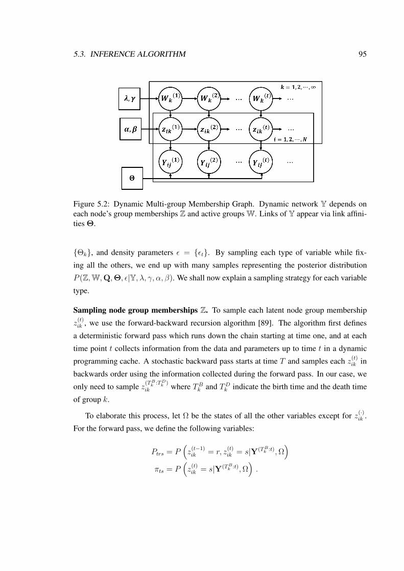
5.3. INFERENCE ALGORITHM 95
Figure 5.2: Dynamic Multi-group Membership Graph. Dynamic network Y depends on
each node’s group memberships Z and active groups W. Links of Y appear via link affini-
ties Θ.
Θk, and density parameters ǫ = ǫt. By sampling each type of variable while fix-
ing all the others, we end up with many samples representing the posterior distribution
P (Z,W,Q,Θ, ǫ|Y, λ, γ, α, β). We shall now explain a sampling strategy for each variable
type.
Sampling node group memberships Z. To sample each latent node group membership
z(t)ik , we use the forward-backward recursion algorithm [89]. The algorithm first defines
a deterministic forward pass which runs down the chain starting at time one, and at each
time point t collects information from the data and parameters up to time t in a dynamic
programming cache. A stochastic backward pass starts at time T and samples each z(t)ik in
backwards order using the information collected during the forward pass. In our case, we
only need to sample z(TB
k :TDk )
ik where TBk and TD
k indicate the birth time and the death time
of group k.
To elaborate this process, let Ω be the states of all the other variables except for z(·)ik .
For the forward pass, we define the following variables:
Ptrs = P(
z(t−1)ik = r, z
(t)ik = s|Y(TB
k :t),Ω)
πts = P(
z(t)ik = s|Y(TB
k :t),Ω)
.

96 CHAPTER 5. MODEL FOR DYNAMIC NETWORKS
We then find the value of each Ptrs and πts through dynamic programming:
πts =∑
r
Ptrs
Ptrs ∝ πt−1,sQk[r, s]P(
Y(t)|z(t)ik = s,Ω)
where Qk =
(
1− ak ak
1− bk bk
)
and∑
r,s Ptrs = 1.
Now given each Ptrs and πts, zTDk
ik can be sampled according to πTDk
, and then the
backward pass samples the z·ik chain backwards:
P(
z(t)ik = r|z(t+1)
ik = s,Y(TBk :TD
k ),Ω)
∝ P(t+1)rs .
Sampling group states W. To update active groups, we use the Metropolis-Hastings algo-
rithm with the following proposal distribution P (W→W′): We add a new group, remove
an existing group, or update the life time of an active group with the same probability 1/3.
When adding a new group k′ we select the birth and death time of the group at random such
that 1 ≤ TBk′ ≤ TD
k′ ≤ T . For removing groups we randomly pick one of existing groups
k′′ and remove it by setting W(t)k′′ = 0 for all t. Finally, to update the birth and death time
of an existing group, we select an existing group and propose new birth and death time of
the group at random. Once new state vector W′ is proposed we accept it with probability
min
(
1,P (Y|W′)P (W′|λ, γ)P (W′→W)
P (Y|W)P (W|λ, γ)P (W→W′)
)
.
We compute P (W|λ, γ) and P (W′ → W) in a closed form, while we approximate the
posterior P (Y|W) by sampling L Gibbs samples while keeping W fixed [?, ?].
Sampling group membership transition matrix Q. Beta distribution is a conjugate prior
of Bernoulli distribution and thus we can sample each ak and bk in Qk directly from the

5.3. INFERENCE ALGORITHM 97
posterior distribution:
ak ∼ Beta(α +N01,k, β +N00,k)
bk ∼ Beta(α +N10,k, β +N11,k)
where Nrs,k is the number of nodes that transition from state r to s in group k (r, s ∈ 0 =
non-member, 1 = member).
Sampling link affinities Θ. Once node group memberships Z are determined, we update
the entries of link affinity matrices Θk. Direct sampling of Θ is intractable because of
non-conjugacy of the logistic link function. An appropriate method in such case would be
the Metropolis-Hastings that accepts or rejects the proposal based on the likelihood ratio.
However, to avoid low acceptance rates and quickly move toward the mode of the posterior
distribution, we develop a method based on Hybrid Monte Carlo (HMC) sampling [23].
We guide the sampling using the gradient of the log-likelihood function with respect to
each Θk. Because links Y(t)ij are generated independently given group memberships Z, the
gradient with respect to Θk[x, y] can be computed by
− 1
2σ2Θ2
k +∑
i,j,t
(
Y(t)ij − p
(t)ij
)
1z(t)ik = x, z(t)jk = y . (5.4)
Updating density parameter ǫ. Parameter vector ǫ is defined over a finite dimension T .
Therefore, we can update ǫ by maximizing the log-likelihood given all the other variables.
We compute the gradient update for each ǫt and directly update ǫt via a gradient step.
Updating hyperparameters. The number of groups over all time periods is given by a
Poisson distribution with parameter λ (1 + γ (T − 1)). Hence, given γ we sample λ by
using a Gamma conjugate prior. Similarly, we can use the Beta conjugate prior for the
group death process (i.e., Bernoulli distribution) to sample γ. However, hyperparameters α
and β do not have a conjugate prior, so we update them by using a gradient method based
on the sampled values of ak and bk [37].

98 CHAPTER 5. MODEL FOR DYNAMIC NETWORKS
Time complexity of model parameter estimation. Last, we briefly comment on the time
complexity of our model parameter estimation procedure. Each sample z(t)ik requires com-
putation of link probability p(t)ij for all j 6= i. Since the expected number of active groups
at each time is λ, this requires O(λN2T ) computations of p(t)ij . By caching the sum of link
affinities between every pair of nodes sampling Z as well as W requires O(λN2T ) time.
Sampling Θ and ǫ also requires O(λN2T ) because the gradient of each p(t)ij needs to be
computed. Overall, our approach takes O(λN2T ) to obtain a single sample, while models
that are based on the interaction matrix between all groups [27,28,39] require O(K2N2T ),
where K is the expected number of groups. Furthermore, it has been shown that O(logN)
groups are enough to represent networks [48, 50]. Thus, in practice K (i.e., λ) is of order
logN and the running time for each sample is O(N2T logN).
5.4 Experiments
We evaluate our model on three different tasks. For quantitative evaluation, we perform
missing link prediction as well as future network forecasting and show our model gives
favorable performance when compared to current dynamic and static network models. We
also analyze the dynamics of groups in a dynamic social network of characters in a movie,
The Lord of the Rings: The Two Towers.
5.4.1 Experimental setup
For the two prediction experiments, we use the following three datasets. First, the NIPS
co-authorships network connects two people if they appear on the same publication in the
NIPS conference in a given year. While this network spans T=17 years (1987 to 2003) [39],
we focus on a subset of 110 most connected people over all time periods. Second, the
DBLP co-authorship network is obtained from 21 Computer Science conferences from
2000 to 2009 (T = 10) [95]. We focus on 209 people by taking 7-core [?] of the aggregated
network for the entire time. Third, the INFOCOM dataset represents the physical proximity
interactions between 78 students at the 2006 INFOCOM conference, recorded by wireless
detector remotes given to each attendee [88]. We use the processed data that removes
inactive time slices to have T=50 [39].

5.4. EXPERIMENTS 99
To evaluate the predictive performance of our model, we compare it to three baseline
models. For a naive baseline model, we regard the relationship between each pair of nodes
as the instance of independent Bernoulli distribution with Beta(1, 1) prior. Thus, for a
given pair of nodes, the link probability at each time equals to the expected probability from
the posterior distribution given network data. The second baseline is the LFRM model [75],
a model of static networks. For missing link prediction, we independently fit LFRM to
each snapshot of dynamic networks. For network forecasting task, we fit LFRM to the
most recent snapshot of a network. Even though LFRM does not capture time dynamics,
we consider this to be a strong baseline model. Finally, for the comparison with dynamic
network models, we consider two recent state of the art models. The DRIFT model [27]
is based on an infinite factorial HMM and authors kindly shared their implementation. We
also consider the LFP model [39] for which we were not able to obtain the implementation,
but since we use the same datasets, we compare performance numbers directly with those
reported in [39].
To evaluate predictive performance, we use various standard evaluation metrics. First,
to assess goodness of inferred probability distributions, we report the log-likelihood of
held-out edges. Second, to verify the predictive performance, we compute the area under
the ROC curve (AUC). Last, we also report the maximum F1-score (F1) by scanning over
all possible precision/recall thresholds.
5.4.2 Task 1: Predicting missing links
To generate the datasets for the task of missing link prediction, we randomly hold out 20%
of node pairs (i.e., either link or non-link) throughout the entire time period. We then run
each model to obtain 400 samples after 800 burn-in samples for each of 10 MCMC chains.
Each sample gives a link probability for a given missing entry, so the final link probability
of a missing entry is computed by averaging the corresponding link probability over all the
samples. This final link probability provides the evaluation metric for a given missing data
entry.
Table 5.1 shows average evaluation metrics for each model and dataset over 10 runs. We
also compute the p-value on the difference between two best results for each dataset and

100 CHAPTER 5. MODEL FOR DYNAMIC NETWORKS
ModelNIPS DBLP INFOCOM
TestLL AUC F1 TestLL AUC F1 TestLL AUC F1
Naive -2030 0.808 0.177 -12051 0.814 0.300 -17821 0.677 0.252
LFRM -880 0.777 0.195 -3783 0.784 0.146 -8689 0.946 0.703
DRIFT -758 0.866 0.296 -3108 0.916 0.421 -6654 0.973 0.757
DMMG −624 0.916 0.434 −2684 0.939 0.492 −6422 0.976 0.764
Table 5.1: Missing link prediction. We bold the performance of the best scoring method.
Our DMMG model performs the best in all cases. All improvements are statistically sig-
nificant at 0.01 significance level.
metric. Overall, our DMMG model significantly outperforms the other models in every
metric and dataset. Particularly in terms of F1-score we gain up to 46.6% improvement
over the other models.
By comparing the naive model and the LFRM model, we observe that the LFRM model
performs especially poorly compared to the naive model in two networks with few edges
(NIPS and DBLP). Intuitively this makes sense because due to the network sparsity we can
obtain more information from the temporal trajectory of each link than from each snapshot
of network. However, both the DRIFT and the DMMG models successfully combine the
temporal and the network information which results in better predictive performance. Fur-
thermore, we note that the DMMG model outperforms the other models by a larger margin
as networks get sparser. The DMMG model makes better use of temporal information
because it can explicitly model temporally local links through active groups.
Last, we also compare our model to the LFP model. The LFP paper reports AUC
ROC score of ∼0.85 for NIPS and ∼0.95 for INFOCOM on the same task of missing link
prediction with 20% held-out missing data [39]. Performance of our DMMG on these same
networks under the same conditions is 0.916 for NIPS and 0.976 for INFOCOM, which is
a strong improvement over the LFP model.
5.4.3 Task 2: Future network forecasting
Here we are given a dynamic network up to time Tobs and the goal is to predict the network
at the next time Tobs + 1. We follow the experimental protocol described in [27, 39]: We
train the models on first Tobs networks, fix the parameters, and then for each model we run

5.4. EXPERIMENTS 101
ModelNIPS DBLP INFOCOM
TestLL AUC F1 TestLL AUC F1 TestLL AUC F1
Naive -547 0.524 0.130 -3248 0.668 0.243 -774 0.673 0.270
LFRM -356 0.398 0.011 -1680 0.492 0.024 -760 0.640 0.248
DRIFT −148 0.672 0.084 −1324 0.650 0.122 -661 0.782 0.381
DMMG -170 0.732 0.196 -1347 0.652 0.245 −625 0.804 0.392
Table 5.2: Future network forecasting. The DMMG model performs best on NIPS and
INFOCOM while results on DBLP are mixed.
MCMC sampling one time step into the future. For each model and network, we obtain
400 samples with 10 different MCMC chains, resulting in 400K network samples. These
network samples provide a probability distribution over links at time Tobs + 1.
Table 5.2 shows performance averaged over different Tobs values ranging from 3 to T -
1. Overall, the DMMG model generally exhibits the best performance, but performance
results seem to depend on the dataset. The DMMG model performs the best at 0.001
significance level in terms of AUC and F1 for the NIPS dataset, and at 0.05 level for the
INFOCOM dataset. While the DMMG model improves performance on AUC (9%) and
F1 (133%), the DRIFT model achieves the best log-likelihood on the NIPS dataset. In
light of our previous observations, we conjecture that this is due to change in network
link density between different snapshots. On the DBLP dataset, the DRIFT model gives
the best log-likelihood, the naive model performs best in terms of AUC, and the DMMG
model is the best on F1 score. However, in all cases of DBLP dataset, the differences are
not statistically significant. Overall, the DMMG model performs the best on NIPS and
INFOCOM and provides comparable performance on DBLP.
5.4.4 Task 3: Case study of “The Lord of the Rings: The Two Towers”
social network
Last, we also investigate groups identified by our model on a dynamic social network of
characters in a movie, The Lord of the Rings: The Two Towers. Based on the transcript
of the movie we created a dynamic social network on 21 characters and T=5 time epochs,
where we connect a pair of characters if they co-appear inside some time window.

102 CHAPTER 5. MODEL FOR DYNAMIC NETWORKS
madrilgaladriel
elrondarwen
faramirhamagrima
theodeneomereowyn
sarumangimli
legolasaragorn
pippingollum
samfrodomerry
gandalfhaldir
1 2 3 4 5
(a) Group 1
madrilgaladriel
elrondarwen
faramirhamagrima
theodeneomereowyn
sarumangimli
legolasaragorn
pippingollum
samfrodomerry
gandalfhaldir
1 2 3 4 5
(b) Group 2
madrilgaladriel
elrondarwen
faramirhamagrima
theodeneomereowyn
sarumangimli
legolasaragorn
pippingollum
samfrodomerry
gandalfhaldir
1 2 3 4 5
(c) Group 3
Figure 5.3: Group arrival and departure dynamics of different characters in the Lord of the
Rings. Dark areas in the plots correspond to a give node’s (y-axis) membership to each
group over time (x-axis)
.
5.5. CONCLUSION 103
We fit our model to this network and examine the results in Figure 5.3. Our model
identified three dynamic groups, which all correspond to the Lord of the Rings storyline.
For example, the core of Group 1 corresponds to Aragorn, elf Legolas, dwarf Gimli, and
people in Rohan who in the end all fight against the Orcs. Similarly, Group 2 corresponds
to hobbits Sam, Frodo and Gollum on their mission to destroy the ring in Mordor, and are
later joined by Faramir and ranger Madril. Interestingly, Group 3 evolving around Merry
and Pippin only forms at t=2 when they start their journey with Treebeard and later fight
against wizard Saruman. While the fight occurs in two separate places we find that some
scenes are not distinguishable, so it looks as if Merry and Pippin fought together with
Rohan’s army against Saruman’s army.
5.5 Conclusion
In this chapter, we presented the Dynamic Multi-group Membership Graph for dynamic
network links, which consider the dynamics both at individual node level and at group
level. In this way we can achieve the joining and leaving of groups for each node as well
as the birth and death for each group. Furthermore, by having the distance-dependent IBP
as a nonparametric prior distribution, the DMMG model also naturally learns the number
of groups at each time.
We developed an MCMC sampling algorithm to infer model parameters for a give dy-
namic network. Based on the inferred model parameters, we can not only predict missing
links but also forecast network links in the future. Experimental results showed that our
model provides better predictive power for the both types of predictive tasks.

104 CHAPTER 5. MODEL FOR DYNAMIC NETWORKS

Chapter 6
Conclusion
6.1 Summary of Contributions
This thesis proposed a family of network models that achieved the following objectives:
• To develop a model that gives rise to networks with common global structural prop-
erties while also permitting a fitting algorithm to capture local link structures.
• To extend the model to incorporate auxiliary information.
In this thesis, we proposed the Multiplicative Attribute Graph (MAG) model in Chap-
ter 3 to achieve the first objective. We then developed two network models that consider
auxiliary information: the Latent Multi-group Membership Graph (LMMG) model for
node features and the Dynamic Multi-group Membership Graph (DMMG) model for tem-
poral information. Each model provides a good probabilistic representation of given data:
network links in the MAG model, network links and node features in the LMMG model,
and a discrete time series of network links in the DMMG model. This probabilistic repre-
sentation improves performance of various prediction tasks compared to the state-of-the-art
models.
Next, we will give the summary for each model in turn.
105

106 CHAPTER 6. CONCLUSION
Model Target of modeling Main focus
MAG Static network links Capturing both global and local structures
LMMG Network links and node features Relationships between links and features
DMMG A discrete time series of network links Two kinds of dynamics
Table 6.1: Summary of the models in this thesis
6.1.1 Summary of our models
We began by proposing the MAG model as a unified generative model that explains the
emergence of global structural properties and offers the statistical inference algorithm to
extract local link structures. We proved several theorems, which include the existence of
giant connected component, small diameter, and heavy-tailed degree distributions. We also
developed a model fitting algorithm that finds the most likely model parameters for given
network links. Using this fitting algorithm, the MAG model is able to represent a given
network in terms of both global structures and local link structures.
The MAG model is extended in two ways: the LMMG model and the DMMG model.
The LMMG model incorporates node features into the generative model so that the model
can represent the relationship between network links and node features. The LMMG model
can enrich the types of prediction tasks, which include the prediction of all the links of a
new node based on its node features even if we do not observe any of the links.
Finally, the DMMG model represents dynamic networks by considering two kinds of
dynamics: group dynamics and individual node dynamics. Inference with both kinds of
dynamics improves performance when predicting missing links and forecasting future net-
work links compared to the state-of-the-art model.
Table 6.1.1 summarizes each model and its main focus.
6.2 Future Work
Now we discuss some future directions of research in the medium term as well as in the
long term.

6.2. FUTURE WORK 107
6.2.1 Medium-term goals
Here we suggest some possible future work, which can be directly extended from our mod-
els.
Communication networks. The dynamic networks modeled in Chapter 5 have a discrete
time series. However, communication networks – such as phone call networks [78, 91]
and message-passing networks like Twitter – are often more dynamic. In communication
networks, each message corresponds to a link and the link is defined only at a certain time or
during a very short time. Practical questions for these networks thus include the prediction
of future messages or the estimation of engagement levels between nodes. Furthermore,
we might be able to detect some signals that imply the emergence or decay of latent groups
in these networks.
Link strength and type. Other extensions of current work include the incorporation of link
type [62] or link strength [70,105]. If each link is annotated by some labels, then we might
be able to find different types of patterns for different labels. For example, while a friend
of a friend is likely to be a friend, an enemy of an enemy is not likely to be an enemy. If
each link is associated with some non-negative value, i.e., link strength, then we may apply
the weak-tie theory [34] and identify critical links bridging different network communities.
In particular, finding such critical links will be useful for increasing the effectiveness of
information propagation [24].
Classification/clustering of networks. Finally, we also propose the classification of net-
works as one avenue for future work. For example, we aim to classify whether a given
network is more like Facebook or Twitter. By incorporating temporal information, we
might determine whether a given network grows or decays, or classify networks by their
different levels of evolution. For instance, in biology we can view the growth of cells
as dynamic networks and determine whether a particular group of cells comprises normal
cells or cancer cells. We can also view this problem in an unsupervised way so that we
cluster similar networks together. We believe that the parameters of models can be used as
important features in classification and clustering.

108 CHAPTER 6. CONCLUSION
6.2.2 Long-term goals
Here we will describe more ultimate goals in modeling networks.
Heterogeneous data. In this thesis, we developed models for homogeneous networks in
which each type of node is the same. However, in general, any kind of relational data can
be viewed as a network. For example, transaction data in online shopping can be regarded
as a bipartite network between purchasers and items. We then address questions such
as: What is the unifying framework for networks with multiple types of entities? Can we
infer missing relationships between two types of entities based on the relationships among
the other types of entities? Answering these questions may require more analysis of this
heterogeneous data, so we leave this problem for long-term future work.
Big data and scalability. In the era of big data, information from networks is often too
rich to incorporate everything at the raw level. For example, many sensors are used to mon-
itor large systems to detect anomalies and find their root causes [52]. Applying complex
network models to this situation will be too expensive due to the large number of sensors
and the massive number of measurements generated by each sensor. Hence, in addition
to developing a “good” model, the scalability of a model needs to be considered as well.
In particular, the raw data from many online web services such as Facebook and LinkedIn
tends to have thousands of entity types (e.g., user, page, ads, and so on) as well as millions
of nodes for each type. Hence, without support for scalability, it would be difficult to rep-
resent the real-world large relational data in a model. Scalability is thus one of the most
essential directions for new research, while finding both good and scalable network models
remains an open research problem.

Appendix A
Table of symbols
SYMBOL DESCRIPTION
V Node set
E Edge set
n,N The number of nodes
m,E The number of edges
Yij An indicator of a link from node i to jY Adjacency matrix
Y(t) Adjacency matrix at time tY(t1:t2) Adjacency matrices from time t1 to time t2Y A collection of adjacency matrices
Θk Link-affinity matrix associated with latent attribute/group kΘ A collection of link-affinity matrices
zik, Zik Membership to latent group k for node iZ Latent group memberships for each node and group
Z(t) Latent group memberships at time tZ(t1:t2) Latent group memberships from time t1 to t2Z A collection of latent group memberships
µk The probability that each node belongs to the k-th latent group/attribute
µ A collection of µk
Fil The l-th feature value of node iF Node feature values for each pair of node and feature
E[·] Expectation
Table A.1: Table of all symbols used in this thesis.
109

110 APPENDIX A. TABLE OF SYMBOLS

Appendix B
Datasets
DATASET N Total E L T DESCRIPTION
LinkedIn 4,096 10,052 - - Online social network
Yahoo-Answers! 4,096 5,678 - - Question-Answer network
AddHealth 458 2,130 35 0 School friendship network
Facebook Ego-network 227 6,348 14 - Ego-network in Facebook
Facebook100 769 33,312 24 - Facebook network of Caltech University
WebKB 195 304 993 - Webgraph of Cornell University webpages
NIPS 110 786 - 17 Coauthorship network
DBLP 209 4,094 - 10 Coauthorship network
INFOCOM 78 28,300 - 50 Physical proximity network
Movie 21 348 - 5 Co-appearance network
Table B.1: Table of all datasets used in this thesis.
111

112 APPENDIX B. DATASETS

Appendix C
Proofs of Theorems
In the appendix we give complete proofs of theorems and lemmas presented earlier in this
thesis. In particular we prove:
• Appendix C.1: The Number of Links. We prove Lemmas 3.3.2, 3.3.3 and Theorem
3.3.1 that we introduced in Section 3.
• Appendix C.2: Connectedness and the Existence of the Giant Component. We prove
Theorems 3.4.1, 3.4.2, and 3.4.3 introduced in Section 3.4.
• Appendix C.3: Diameter. We prove Lemmas 3.5.2 and 3.5.3 described in Section
3.5.
• Appendix C.4: Log-Normal Degree Distribution. We prove Theorem 3.6.1 from
Section 3.6.
• Appendix C.5: Power-law Degree Distribution. We prove Lemmas 7.2, 7.3, and
Theorem 3.7.1 described in Section 3.7.
C.1 Appendix: The number of links
Here we describe all the proofs with regard to the number of links in M(n, k, µ,Θ) as
shown in Section 3.3.2.
To prove Theorem 3.3.1, the following two lemmas are required:
113

114 APPENDIX C. PROOFS OF THEOREMS
Lemma C.1.1. The expected link probability between distinct nodes u and v is
E [P [u, v] |u ∈ Wi] = (µα+ (1− µ)β)i (µβ + (1− µ)γ)k−i .
Proof of Lemma C.1.1: Let N0uv be the number of attributes that take value 0 in both u
and v. For instance, if a(u) = [0 0 1 0] and a(v) = [0 1 1 0], then N0uv = 2. We similarly
define N1uv as the number of attributes that take value 1 in both u and v. Then, N0
uv, N1uv ≥ 0
and N0uv +N1
uv ≤ k as k indicates the number of attributes in each node.
By definition of MAG model, the edge probability between u and v is
P [u, v] = αN0uvβk−N0
uv−N1uvγN1
uv .
Since both N0uv and N1
uv are random variables, we need their conditional joint distribu-
tion to compute the expectation of the edge probability P [u, v] given the weight of node u.
Note that N0uv and N1
uv are independent of each other if the weight of u is given. Let the
weight of u be i, which means that u ∈ Wi. Since u and v can share value 0 only for the
attributes where u already takes value 0, N0uv equivalently represents the number of heads
in i coin flips with probabilty µ. Therefore, N0uv follows Bin(i, µ). Similarly, N1
uv follows
Bin(k − i, 1− µ). Hence, their conditional joint probability is
P (N0uv, N
1uv|u ∈ Wi) =
(
i
N0uv
)
µN0uv(1− µ)i−N0
uv
(
k − i
N1uv
)
µk−i−N1uv(1− µ)N
1uv .
Using this conditional probability, we can compute the expectation of P [u, v] given the
weight of u:
E [P [u, v] |u ∈ Wi] = E
[
αN0uvβi−N0
uvβk−i−N1uvγN1
uv |u ∈ Wi
]
=
i∑
N0uv=0
k−i∑
N1uv=0
(
i
N0uv
)(
k − i
N1uv
)
(αµ)N0uv ((1− µ)β)i−N0
uv (µβ)k−i−N1uv ((1− µ)γ)N
1uv
=
i∑
N0uv=0
(
i
N0uv
)
(αµ)N0uv ((1− µ)β)i−N0
uv
k−i∑
N1uv=0
(
k − i
N1uv
)
(µβ)k−i−N1uv ((1− µ)γ)N
1uv
= (µα + (1− µ)β)i (µβ + (1− µ)γ)k−i .

C.1. APPENDIX: THE NUMBER OF LINKS 115
Lemma C.1.2. The expected degree of node u for its given weight i is
E [deg(u)|u ∈ Wi] = (n− 1) (µα + (1− µ)β)i (µβ + (1− µ)γ)k−i + 2αiγk−i .
Proof of Lemma C.1.2: By Lemma C.1.1 and the linearity of expectation, we sum this
conditional probability over all nodes and result in the expectation of the degree given the
weight of node u.
Using the above lemmas, we then prove Theorem 3.3.1:
Proof of Theorem 3.3.1: We compute the expected number of links, written as E [m], by
adding up the degrees of all nodes described in Lemma C.1.2,
E [m] = E
[
1
2
∑
u∈V
deg(u)
]
=1
2n
k∑
j=0
P (Wj)E [deg(u)|u ∈ Wj ]
=1
2n
k∑
j=0
(
k
j
)
µj(1− µ)k−jE [deg(u)|u ∈ Wj ]
=1
2n
k∑
j=0
(
k
j
)
(
(n− 1) (µα + (1− µ)β)j (µβ + (1− µ)γ)k−j + 2αjµjγk−j(1− µ)k−j)
=n(n− 1)
2
(
µ2α + 2µ(1− µ)β + (1− µ)2γ)k
+ n (µα + (1− µ)γ)k .
Proof of Corollary 3.3.1.1: Suppose that k =(
ǫ− 1log ζ
)
log n for ζ = µ2α + 2µ(1 −µ)β + (1− µ)2γ and ǫ > 0. By Theorem 3.3.1, the expected number of links is Θ
(
n2ζk)
.
Note that log ζ < 0 since ζ < 1. Therefore, the expected number of links is
Θ(n2ζk) = Θ(
ζk+2 log nlog ζ
)
= Θ(n1+ǫ log ζ) = o(n) .
Proof of Corollary 3.3.1.2: Under the situation that k ∈ o(logn), the expected number of
links is
Θ(n2ζk) = Θ(n2+( klog n
) log ζ) = Θ(n2+o(1) log ζ) = Θ(n2−o(1)) .

116 APPENDIX C. PROOFS OF THEOREMS
C.2 Appendix: Connectedness and Giant Connected Com-
ponent
Since Theorem 3.3.2 is used to prove other theorems, we begin with the proof of it.
Proof of Theorem 3.3.2: If j ≥ i, for any v ∈ Wi, we can generate a node v(j) ∈ Wj
from v by flipping (j − i) attribute values that originally take 1 in v. For example, if
a(v) = [0 1 1 0], then a(v(3)) = [0 0 1 0] or [0 1 0 0]. Hence, P [u, v(j)] ≥ P [u, v] for
v ∈ Wi.
Here we note that E[
P[
u, v(j)]
|v ∈ Wi
]
= E[
P[
u, v(j)]
|v(j) ∈ Wj
]
, because each
v(j) can be generated by(
ji
)
different a(v) sets with the same probability. Therefore,
E [P [u, v] |v ∈ Wj ] = E[
E[
P[
u, v(j)]
|v ∈ Wi
]]
≥ E [E [P [u, v] |v ∈ Wi]] = E [P [u, v] |v ∈ Wi] .
Now we introduce the theorem which plays a key role in proving Theorem 3.3.3 as well
as Theorem 3.3.4.
Theorem C.2.1. Let |Sj| ∈ Θ(n) and E [P [u,V\u] |u ∈ Wj ] ≥ c logn as n → ∞ for
some j and sufficiently large c. Then, Sj is connected almost surely as n→∞.
Proof: Let S ′ be a subset of Sj such that S ′ is neither an empty set nor Sj itself. Then, the
expected number of links between S ′ and Sj\S ′ is
E [P [S ′, Sj\S ′] | |S ′| = k] = k · (|Sj| − k) · E [P [u, v] |u, v ∈ Sj ]
for distinct u and v. By Theorem 3.3.2,
E [P [u, v] |u, v ∈ Sj] ≥ E [P [u, v] |u ∈ Sj , v ∈ V]≥ E [P [u, v] |u ∈ Wj , v ∈ V\u]
≥ c logn
n.
Given the size of S ′ as k, the probability that there exists no edge between S ′ and Sj\S ′
is at most exp(
−12E [P [S ′, Sj\S ′] ||S ′| = k]
)
by the Chernoff bound [85]. Therefore, the
probability that Sj is disconnected is bounded as follows:

C.2. APPENDIX: CONNECTEDNESS AND GIANT CONNECTED COMPONENT117
P (Sj is disconnected) ≤∑
S′⊂Sj ,S′ 6=∅,Sj
P (no edge between S ′, Sj\S ′)
≤∑
S′⊂S,S′ 6=∅,Sj
exp
(
−12E [P [S ′, Sj\S ′] ||S ′|]
)
≤∑
S′⊂S,S′ 6=∅,Sj
exp
(
−|S ′| (|Sj| − |S ′|) c log n2n
)
≤ 2∑
1≤k≤|Sj|/2
(|Sj |i
)
exp
(
−c|Sj | logn4n
k
)
≤ 2∑
1≤k≤|Sj|/2
|Sj|k exp(
−c|Sj | logn4n
k
)
≤ 2∑
1≤k≤|Sj|/2
exp
((
log |Sj| −c|Sj| logn
4n
)
k
)
= 2∑
1≤k≤|Sj|/2
exp (−kΘ(log n)) (∵ |Sj| ∈ Θ(n))
= 2∑
1≤k≤|Sj|/2
(
1
nΘ(1)
)k
≈ 1
nΘ(1)∈ o(1)
as n→∞. Therefore, Sj is connected almost surely.
C.2.1 Existence of the giant connected component
Now we turn our attention to the giant connected component. To show its existence, we
investigate Sµk, Sµk+k1/6 , and Sµk+k2/3 depending on the situation. The following lemmas
tell us the size of each subgraph.
Lemma C.2.2. |Sµk| ≥ n2− o(n) almost surely as n→∞.
Proof: By the Central Limit Theorem [85],|u|−µk√kµ(1−µ)
∼ N(0, 1) as n → ∞, that is,
k →∞. Therefore, P (|u| ≥ µk) is at least 12− o(1) so |Sµk| ≥ n
2− o(n) almost surely as
n→∞.

118 APPENDIX C. PROOFS OF THEOREMS
Lemma C.2.3. |Sµk+k1/6| ∈ Θ(n) almost surely as n→∞.
Proof: By the Central Limit Theorem mentioned in Lemma C.2.2,
P (µk ≤ |u| < µk + k1/6) ≈ Φ(k1/6
√
kµ(1− µ))− Φ(0) ∈ o(1)
as k →∞ where Φ(z) represents the cdf of the standard normal distribution.
Since P (|u| ≥ µk+k1/6) is still at least 12−o(1), the size of Sµk+k1/6 is Θ(n) almost surely
as k →∞, that is, n→∞.
Lemma C.2.4. |Sµk+k2/3| ∈ o(n) almost surely as n→∞.
Proof: By the Chernoff bound, P (|u| ≥ µk + k2/3) is o(1) as k → ∞, thus |Sµk+k2/3| iso(n) almost surely as n→∞.
Proof of Theorem 3.3.3: (Existence) First, if[
(µα + (1− µ)β)µ (µβ + (1− µ)γ)1−µ]ρ >12, then by Lemma C.1.2,
E [P [u,V\u] |u ∈ Wµk] ≈[
2[
(µα+ (1− µ)β)µ (µβ + (1− µ)γ)1−µ]ρ]logn
= (1 + ǫ)logn > c logn
for some constant ǫ > 0 and c > 0. Since |Sµk| ∈ Θ(n) by Lemma C.2.2, Sµk is connected
almost surely as n → ∞ by Theorem C.2.1. In other words, we are able to extract out a
connected component of size at least n2− o(n).
Second, when[
(µα + (1− µ)β)µ (µβ + (1− µ)γ)1−µ]ρ = 12, we can apply the same
argument for Sµk+k1/6 . Because |Sµk+k1/6 | ∈ Θ(n) by Lemma C.2.3,
E[
P [u,V\u] |u ∈ Wµk+k1/6]
≈[
2[
(µα + (1− µ)β)µ (µβ + (1− µ)γ)1−µ]ρ]logn
(
µα + (1− µ)β
µβ + (1− µ)γ
)(ρ logn)1/6
=
(
µα + (1− µ)β
µβ + (1− µ)γ
)(ρ logn)1/6
= (1 + ǫ′)ρ logn1/6

C.2. APPENDIX: CONNECTEDNESS AND GIANT CONNECTED COMPONENT119
which is also greater than c logn as n → ∞ for some constant ǫ′ > 0. Thus, Sµk+k1/6 is
connected almost surely by Theorem C.2.1.
Last, on the contrary, when[
(µα+ (1− µ)β)µ (µβ + (1− µ)γ)1−µ]ρ < 12, for u ∈
Wµk+k2/3 ,
E[
P [u,V\u] |u ∈ Wµk+k2/3
]
≈[
2[
(µα+ (1− µ)β)µ (µβ + (1− µ)γ)1−µ]ρ]logn
(
µα + (1− µ)β
µβ + (1− µ)γ
)(ρ logn)2/3
=
[
(1− ǫ′′)ρ−2/3(log n)1/3
(
µα+ (1− µ)β
µβ + (1− µ)γ
)](ρ logn)2/3
is o(1) as n → ∞ for some constant ǫ′′ > 0. Therefore, by Theorem 3.3.2, the expected
degree of a node with weight less than µk + k2/3 is o(1). However, since Sµk+k2/3 is o(n)
by Lemma C.2.4, n−o(n) nodes have less than µk+k2/3 weights. Hence, most of n−o(n)nodes are isolated so that the size of the largest component cannot be Θ(n).
C.2.2 Uniqueness of the largest connected component
We already pointed out that either Sµk or Sµk+k1/6 is the subset of Θ(n) component when
the giant connected component exists. Let this component be H . Without loss of generality,
suppose that Sµk ⊂ H . Then, for any fixed node u,
P [u,H ] ≥ P [u, Sµk] (∵ Sµk ⊂ H)
= |Sµk| · E [P [u, v] |v ∈ Sµk]
≥ |Sµk| · E [P [u, v] |v ∈ V\Sµk] (By Theorem 3.3.2)
=|Sµk|
n− |Sµk|P [u,V\Sµk]
Since V\H ⊂ V\Sµk,
E [P [u,V\H]] ≤ E [P [u,V\Sµk]] ≤(
n− |Sµk||Sµk|
)
E [P [u,H]]
holds for every u ∈ V .

120 APPENDIX C. PROOFS OF THEOREMS
Suppose that another connected component H ′ also contains Θ(n) nodes. We will
show the contradiction if H and H ′ are not connected almost surely as n → ∞. To see
E [P [H,H ′]],
E [P [H,H ′]] = |H ′| · E [P [u,H] |u ∈ H ′]
≥ |H′| · |Sµk|
n− |Sµk|E [P [u,V\Sµk] |u ∈ H ′]
≥ |H′| · |Sµk|
n− |Sµk|E [P [u,H ′] |u ∈ H ′] (∵ H ′ ⊂ V\H ⊂ V\Sµk) .
However, E [P [u,H ′] |u ∈ H ′] ∈ Ω(1). Otherwise, since the probability that u ∈ H ′ is
connected to H ′ is not greater than E [P [u,H ′] |u ∈ H ′] by Markov Inequality [85], u is
disconnected from H ′ almost surely as n→∞. H ′ thus includes at least one isolated node
almost surely as n→∞. This is contradiction to the connectedness of H ′.
On the other hand, if E [P [u,H ′] |u ∈ H ′] ∈ Ω(1), then E [P [H,H ′]] ∈ Ω(n). In this
case, by the Chernoff bound, H and H ′ are connected almost surely as n → ∞. This is
also contradiction. Therefore, there is no Θ(n) connected component other than H almost
surely as n→∞.
C.2.3 Conditions for the connectedness of a MAG network
Next, the proofs for the connectedness follow. Before the main proof, we present an essen-
tial lemma and prove it.
Lemma C.2.5. If (1 − µ)ρ ≥ 12, then Vmin
k→ 0 almost surely as n → ∞. Otherwise, if
(1 − µ)ρ < 12, Vmin
k→ ν almost surely as n → ∞, where ν is a solution of the equation
[
(
µν
)ν (1−µ1−ν
)1−ν]ρ
= 12
in (0, µ).
Proof: First, we assume that (1 − µ)ρ ≥ 12, which indicates n(1 − µ)ρ ≥ 1 by definition.
Then, the probability that |Wi| = 0 is at most exp(−12E [|Wi|]) by the Chernoff bound.
However, for fixed µ,
E [|W1|] = n
(
k
1
)
µ1(1− µ)k−1 ≥ µ
1− µk ∈ O(k) .

C.2. APPENDIX: CONNECTEDNESS AND GIANT CONNECTED COMPONENT121
Therefore, by the Chernoff bound, P (|W1| = 0)→ 0 as k →∞. This implies that Vmin is
o(k) almost surely as n→∞.
Second, we look at the case that (1− µ)ρ < 12. For any ǫ ∈ (0, µ− ν), to use Stirling’s
approximation,
E[
|W(ν+ǫ)k|]
≈ n
(
k
(ν + ǫ)k
)
µ(ν+ǫ)k(1− µ)(1−(ν+ǫ))k
≈√2πk(k
e)k
√
2π(ν + ǫ)k( (ν+ǫ)ke
)(ν+ǫ)k√
2π(1− (ν + ǫ))(
(1−(ν+ǫ))ke
)(1−(ν+ǫ))k
× nµ(ν+ǫ)k(1− µ)(1−(ν+ǫ))k
=n
√
2πk(ν + ǫ) (1− (ν + ǫ))
[
(
µ
ν + ǫ
)ν+ǫ(1− µ
1− (ν + ǫ)
)1−(ν+ǫ)]k
.
Since(
µx
)x (1−µ1−x
)1−xis a increasing function of x over (0, µ),
(
µ
ν + ǫ
)ν+ǫ(1− µ
1− (ν + ǫ)
)1−(ν+ǫ)
= (1 + ǫ′)
(
1
2
)1/ρ
= (1 + ǫ′)n−1/k
for some constant ǫ′ > 0. Therefore,
E[
|W(ν+ǫ)k|]
=(1 + ǫ′)k
√
2πk(ν + ǫ) (1− (ν + ǫ))
exponentially increases as k increases. By the Chernoff bound, |W(ν+ǫ)k| is not zero almost
surely as k →∞; that is, n→∞.
In a similar way, E[
|W(ν−ǫ)k|]
= (1−ǫ′)k√2πk(ν−ǫ)(1−(ν−ǫ))
exponentially decreases as k in-
creases. Since E [|Wi|] ≥ E [|Wj|] if µk ≥ i ≥ j, the expected number of nodes with at
most weight (ν−ǫ)l is less than (ν−ǫ)k E[
|W(ν−ǫ)k|]
and its value goes to zero as k →∞.
Hence, by the Chernoff bound, there exists no node of the weight less than (ν− ǫ)k almost
surely as n→∞.
To sum up, Vmin
kgoes to ν almost surely as k →∞; that is, n→∞.
Using the above lemma, we show the condition that the network is connected.

122 APPENDIX C. PROOFS OF THEOREMS
Proof of Theorem 3.3.4: Let Vmin
k→ t for a constant t ∈ [0, µ) as n→∞.
If[
(µα + (1− µ)β)t (µβ + (1− µ)γ)1−t]ρ > 12, by Lemma C.1.2,
E [P [u,V\u] |u ∈ WVmin] ≈ E [P [u,V\u] |u ∈ Wtk]
≈[
2[
(µα+ (1− µ)β)t (µβ + (1− µ)γ)1−t]ρ]logn
= (1 + ǫ)logn
≥ c logn
for some ǫ > 0 and sufficiently large c. Note that SVminindicates the entire network by
definition of Vmin. Since |SVmin| is Θ(n), SVmin
is connected almost surely as n → ∞ by
Theorem C.2.1. Equivalently, the entire network is also connected almost surely n→∞.
On the other hand, when (µα + (1− µ)β)Vminlogn (µβ + (1− µ)γ)
k−Vminlog n < 1
2, the ex-
pected degree of a node with |Vmin| weight is o(1) because from the above relationship
E [P [u,V\u] |u ∈ WVmin] ≈ (1 − ǫ′)logn for some ǫ′ > 0. Thus, in this case, some node in
WVminis isolated almost surely so the network is disconnected.
C.3 Appendix: Diameter
Here we first introduce the theorem which plays a key role in showing the constant di-
ameter in the MAG model, and then the proofs of Lemmas 3.3.6 and 3.3.7 described in
Section 3.3.4 follow.
Theorem C.3.1. [9, 17] For an Erdos-Renyi random graph G(n, p), if (pn)d−1/n → 0
and (pn)d/n → ∞ for a fixed integer d, then G(n, p) has diameter d with probability
approaching 1 as n→∞.
Proof of Lemma 3.3.6: Let AG and AH be the probabilistic adjacency matrices of random
graphs G and H , respectively. If AGij ≥ AH
ij for every i, j and H has a bounded diameter
almost surely, then so does G. It can be understood in the following way. To generate a
network with AG, we first generate links with AH and further create links with (AG−AH).
However, as the links created in the first step already result in the constant diameter almost
surely, G has a constant diameter.

C.3. APPENDIX: DIAMETER 123
Note that minu,v∈SλkP [u, v] ≥ βλkγ(1−λ)k. Thus, it is sufficient to prove that the Erdos-
Renyi random graph G(|Sλk|, βλkγ(1−λ)k) has a constant diameter almost surely as n→∞.
However,
E [|Wλk|] βλkγ(1−λ)k = n
(
k
λk
)
µλk(1− µ)(1−λ)kβλkγ(1−λ)k
≈ n√
2πkλ (1− λ)
(
µβ
λ
)λk ((1− µ)γ
1− λ
)(1−λ)k
(By Stirling approximation
=n
√
2πkλ (1− λ)(µβ + (1− µ)γ)k (∵ λ =
µβ
µβ + (1− µ)γ)
=1
√
2πkλ (1− λ)(2 (µβ + (1− µ)γ)ρ)
logn
=1
√
2πkλ (1− λ)(1 + ǫ)logn
for some ǫ > 0.
Since this value goes to infinity as n→∞, so does E [Wλk]. Therefore, by the Chernoff
bound, |Wλk| ≥ cE [Wλk] almost surely as n→∞ for some constant c. Then,
|Sλk|βλkγ(1−λ)k ≥ |Wλk|βλkγ(1−λ)k
≥ cE [|Wλk|] βλkγ(1−λ)k
≈ c√
2πkλ (1− λ)(1 + ǫ)logn .
By Theorem C.3.1, an Erdos-Renyi random graph G(|Sλk|, c(1+ǫ)log n
|Sλk|√
2πkλ(1−λ)) has a diam-
eter of at most(
1 + ln 2ǫ
)
almost surely as n→∞. Thus, the diameter of G(|Sλk|, βλkγ(1−λ)k)
as well as Sλk is also bounded by a constant almost surely as n→∞.

124 APPENDIX C. PROOFS OF THEOREMS
Proof of Lemma 3.3.7: For any u ∈ V ,
P [u, Sλk] ≥k∑
j=λk
n
(
k
j
)
µj(1− µ)k−jβjγk−j
=k∑
j=λk
n
(
k
j
)
λj(1− λ)k−j
(
µβ
λ
)j ((1− µ)γ
1− λ
)k−j
=
k∑
j=λk
n
(
k
j
)
λj(1− λ)k−j (µβ + (1− µ)γ)k
= (2 (µβ + (1− µ)γ)ρ)logn
(
k∑
j=λk
(
k
j
)
λj(1− λ)k−j
)
.
By the Central Limit Theorem,∑k
j=λk
(
kj
)
λj(1 − λ)k−j converges to 12
as k → ∞. There-
fore, P [u, Sλk] is greater than c logn for a constant c, and then, by the Chernoff bound, u
is directly connected to Sλk almost surely as n→∞.
C.4 Appendix: Log-Normal Degree Distribution
First we introduce a general formula of degree distribution in any random graph model.
Theorem C.4.1. [109]P (deg(u) = d) =∫
u∈V
(
n−1d
)
(E [P [u, v]])d (1− E [P [u, v]])n−1−d du.
If we plug the M(n, k, µ,Θ) into the above theorem, we result in the following corollary.
Corollary C.4.1.1. For Ej = (µα + (1− µ)β)j (µβ + (1− µ)γ)k−j,
the probability of degree d in M(n, k, µ,Θ) is pd =∑k
j=0
(
kj
)
µj(1−µ)k−j(
n−1d
)
Edj (1−Ej)
n−1−d.
Proof: We reformulate the statement of Theorem C.4.1,
P (deg(u) = d) =
k∑
j=0
P (u ∈ Wj)
(
n− 1
d
)
(E [P [u, v] |u ∈ Wj])d (1− E [P [u, v] |u ∈ Wj])
n−1−d .
and, by applying Lemma C.1.1, we obtain the desired formula.

C.4. APPENDIX: LOG-NORMAL DEGREE DISTRIBUTION 125
Now we prove the main theorem of degree distribution for M(n, k, µ,Θ), using the
above corollary.
Proof of Theorem 3.3.8: To reduce space, we begin by defining shorthand notation for
various quantities as follows:
x = µα+ (1− µ)β
y = µβ + (1− µ)γ
fj(d) =
(
n− 1
d
)
(
xjyk−j)d (
1− xjyk−j)n−1−d
gj(d) =
(
k
j
)
µj(1− µ)k−jfj(d) .
By Corollary C.4.1.1, we can restate pd as∑l
j=0 gj(d).
If most of those terms turn out to be insignificant under our assumptions, the probability
pd can be approximately proportional to one or few dominant terms. In this case, what we
need to do is thus to seek for j that maximizes gj(d) =(
kj
)
µj(1 − µ)k−jfj(d) and find its
approximate formula.
We start with the approximation of fj(d). For large n and d, by Stirling approximation,
fj(d) ≈√2πn(n/e)n
(
xjyk−j)d (
1− xjyk−j)n−d
√2πd(d/e)d
√
2π(n− d) ((n− d)/e)n−d
=1
√
2πd(
1− dn
)
(
nxjyk−j
d
)d(1− xjyk−j
1− d/n
)n−d
.
However, the expected degree of maximum weight node is O(n (µα + (1− µ)β)k), so
is the expected maximum degree. d is thus o(n) almost surely as n→∞, that is, k →∞.
Therefore,
(
1− xjyk−j
1− d/n
)n−d
≈ exp(
−(n− d)xjyk−j + (n− d)d/n)
≈ exp(−nxjyk−j + d) .

126 APPENDIX C. PROOFS OF THEOREMS
For sufficiently large k, we can further simplify gj(d) by normal approximation of the
binomial distribution:
ln gj(d) = ln
(
k
j
)
µj(1− µ)k−j + ln fj(d)
≈ −12ln (2πkµ(1− µ))− 1
2kµ(1− µ)(j − µk)2 + ln fj(d)
≈ C − 1
2kµ(1− µ)(j − µk)2 − 1
2ln d− d ln
d
nxjyk−j+ d
(
1− nxjyk−j
d
)
for some constant C. When d = nxτyk−τ for τ ≥ µk and R = xy,
ln gj(d) ≈ C − 1
2kµ(1− µ)(j − µk)2 − 1
2ln d+ d(j − τ) lnR + d
(
1−Rj−τ)
.
Using (j − µk)2 = (j − τ)2 + (τ − µk)2 + 2(j − τ)(τ − µk),
ln gj(d) ≈ Cτ −(j − τ)2
2kµ(1− µ)+ (j − τ)
(
d lnR− τ − µk
kµ(1− µ)
)
+ d(
1−Rj−τ)
− 1
2ln d
for Cτ = C − (τ−µk)2
2kµ(1−µ).
Considering gj(d) as a function of j, not d, now we find j that maximizes gj(d) for
d = nxτyk−τ . However, the median weight is approximately equal to µk by the Central
Limit Theorem. If we focus on the higher half degrees we can then let τ ≥ µk. And in this
case, since[
(µα + (1− µ)β)µ (µβ + (1− µ)γ)1−µ]ρ > 12,
∴ d ≥[
(µα+ (1− µ)β)µ (µβ + (1− µ)γ)1−µ]ρ ∈ Ω(k) .
If we differentiate ln gj(d) with respect to j,
(ln gj(d))′ ≈ − j − τ
kµ(1− µ)+
(
d lnR− τ − µk
kµ(1− µ)
)
− dRj−τ lnR = 0 .
Because d ∈ Ω(k) and j, τ ∈ O(k), we can conclude that Rj−τ ≈ 1 as n→∞; other-
wise, | (ln gj(d))′ | grows as large as Ω(d). Therefore, when j ≈ τ , gj(d) is maximized.
C.5. APPENDIX: POWER-LAW DEGREE DISTRIBUTION 127
Furthermore, since | j−τ2kµ(1−µ)
| ≪ d lnR as n → ∞, the first quadratic term(j−τ)2
2kµ(1−µ)in
ln gj(d) is negligible. As a result, when R is practical (close to 1.6 ∼ 3), ln gτ+∆ would be
at most (Θ(−d|∆|)− ln gτ) for ∆ ≥ 1. After all, gτ effectively dominates the probability
pd, so ln pd is roughly proportional to ln gτ . By assigning τ = ln d−lnnyk
lnR, we obtain
ln pd ≈ C − 1
2kµ(1− µ)
(
ln d− lnnyk
lnR− µk
)2
− 1
2ln d
= C ′ − 1
2kµ(1− µ)(lnR)2
(
ln d− lnnyk − kµ lnR− 1
2kµ(1− µ)(lnR)2
)2
.
for some constant C ′. Therefore, the degree distribution pd approximately follows the log-
normal as described in Theorem 3.3.8.
C.5 Appendix: Power-law Degree Distribution
In order to investigate the degree distribution of M(n, k,µ,Θ), the following two lemmas
are essential.
Lemma C.5.1. The probability that node u in M(n, k,µ,Θ) has a latent attribute vector
with values ai(u) (for i = 1, . . . , k) is
k∏
i=1
(µi)1ai(u)=0(1− µi)
1ai(u)=1 .
Proof of Lemma C.5.1: Since ai’s are independently distributed Bernoulli random vari-
ables, Lemma C.5.1 holds.
Lemma C.5.2. The expected degree of node u in M(n, k,µ,Θ) is
(n− 1)k∏
i=1
(µiαi + (1− µi)βi)1ai(u)=0 (µiβi + (1− µi) γi)
1ai(u)=1 .

128 APPENDIX C. PROOFS OF THEOREMS
Proof of Lemma C.5.2: Let’s define Pj(u, v) as the edge probability between u and v
when considering only up to the j-th attribute:
Pj(u, v) =
j∏
i=1
Θi [ai(u), ai(v)] .
Thus, what we aim to show is that for a node v,
E [Pk(u, v)] =k∏
i=1
(µiαi + (1− µi)βi)1ai(u)=0 (µiβi + (1− µi)γi)
1ai(u)=1 .
When k = 1, it is trivially true by Lemma C.1.1. When k > 1, suppose that the above
formula holds for k = 1, 2, · · · , k′. Since Pk′+1(u, v) = Pk′(u, v)Θk′+1 [ak′+1(u), ak′+1(v)],
E [Pk′+1(u, v)]
= E [Pk′(u, v)]E [Θk′+1[ak′+1(u), ak′+1(v)]]
= E [Pk′(u, v)] (µk′+1αk′+1 + (1− µk′+1)βk′+1)1ak′+1(u)=0(µk′+1βk′+1 + (1− µk′+1)γk′+1)
1ak′+1(u)=1
=k′+1∏
i=1
(µiαi + (1− µi)βi)1ai(u)=0 (µiβi + (1− µi)γi)
1ai(u)=1 .
Hence, the expected degree formula described in Lemma C.5.2 holds for every k ≥ 1.
By Lemma C.5.1 and C.5.2, if the condition in Theorem 3.3.9 holds, the probability
that a node has the same feature vector as node u is proportional to (−δ)-th power of the
expected degree of u. In addition, (−12)-th power comes from the Stirling approximation
for large k. This roughly explains Theorem 3.3.9.
Applying the above lemmas into Theorem C.4.1, we show the degree distribution of
M(n, k,µ,Θ) as described in Theorem 3.3.9.
Proof of Theorem 3.3.9: Before the main argument, we need to define the ordered proba-
bility mass of attribute vectors as p(j) for j = 1, 2, · · · , 2k. For example, if the probability
of each attribute vector (00, 01, 10, 11) is respectively 0.2, 0.3, 0.4, and 0.1 when k = 2, the
ordered probability mass is p(1) = 0.1, p(2) = 0.2, p(3) = 0.3, and p(4) = 0.4.
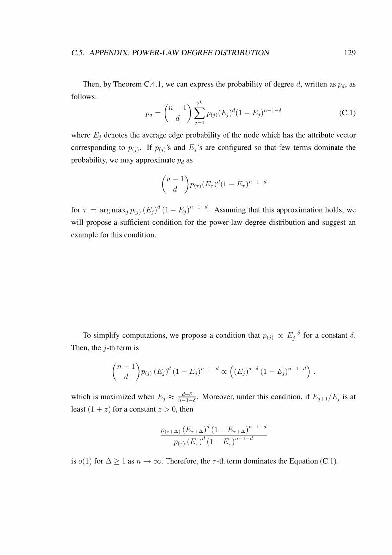
C.5. APPENDIX: POWER-LAW DEGREE DISTRIBUTION 129
Then, by Theorem C.4.1, we can express the probability of degree d, written as pd, as
follows:
pd =
(
n− 1
d
) 2k∑
j=1
p(j)(Ej)d(1− Ej)
n−1−d (C.1)
where Ej denotes the average edge probability of the node which has the attribute vector
corresponding to p(j). If p(j)’s and Ej’s are configured so that few terms dominate the
probability, we may approximate pd as
(
n− 1
d
)
p(τ)(Eτ )d(1−Eτ )
n−1−d
for τ = argmaxj p(j) (Ej)d (1− Ej)
n−1−d. Assuming that this approximation holds, we
will propose a sufficient condition for the power-law degree distribution and suggest an
example for this condition.
To simplify computations, we propose a condition that p(j) ∝ E−δj for a constant δ.
Then, the j-th term is
(
n− 1
d
)
p(j) (Ej)d (1− Ej)
n−1−d ∝(
(Ej)d−δ (1− Ej)
n−1−d)
,
which is maximized when Ej ≈ d−δn−1−δ
. Moreover, under this condition, if Ej+1/Ej is at
least (1 + z) for a constant z > 0, then
p(τ+∆) (Eτ+∆)d (1− Eτ+∆)
n−1−d
p(τ) (Eτ )d (1− Eτ )
n−1−d
is o(1) for ∆ ≥ 1 as n→∞. Therefore, the τ -th term dominates the Equation (C.1).

130 APPENDIX C. PROOFS OF THEOREMS
Next, by the Stirling approximation with the above conditions,
pd ≈(
n− 1
d
)(
d− δ
n− 1− δ
)d−δ (n− 1− d
n− 1− δ
)n−1−d
∝ 1√
d(n− 1− d)(d− δ)−δ
(
(n− 1)(d− δ)
d(n− 1− δ)
)d(n− 1
n− 1− δ
)n−1−d
∝ d−1/2 (d− δ)−δ
(
1− δ
d
)d
≈ d−δ−1/2 exp(−δ)
for sufficiently large d and n. Thus, pd is approximately proportional to d−12−δ for large d
as n→∞.
Last, we prove that the two conditions for the power-law degree distribution are simul-
taneously feasible by providing an example configuration.
If every p(j) is distinct and µi
1−µi=(
µiαi+(1−µi)βi
µiβi+(1−µi)γi
)−δ
, then we satisfy the condition
that p(j) ∝ (Ej)−δ by Lemma C.5.1 and Lemma C.5.2. On the other hand, if we set
µi
1−µi= (1 + z)−2iδ
, then the other condition, Ej+1/Ej ≥ (1 + z) is also satisfied. Since
we are free to configure µi’s and Θi’s independently, the sufficient condition for the power
law degree distribution is satisfied.

Appendix D
Details of the MAGFIT Algorithm
D.1 Details of Variational EM Algorithm
In Section 3.4.1, we proposed a version of MAG model with a generative Bernoulli model
for node attributes, formulated the problem to solve. In Section 3.4.2, we gave a sketch
of MAGFIT using the variational EM algorithm. Here we provide additional details on
computing the gradients of the model parameters (Φ, µ, and Θ) for the E-step and M-step
of the variational algorithm. We also give the details on the fast version of MAGFIT.
D.1.1 Variational E-Step
In the E-step, the MAG model parameters µ and Θ are given and we aim to find the optimal
variational parameter Φ that maximizes LQ(µ,Θ) as well as minimizes the mutual infor-
mation factor MI(Z). We randomly select a batch of entries in Φ and update the selected
entries by their gradient values of the objective function LQ(µ,Θ). We repeat this updating
procedure until Φ converges.
To obtain∇Φ (LQ(µ,Θ)− λMI(Z)), we compute∂LQ
∂φiland ∂MI
∂φilin turn as follows.
Computation of∂LQ
∂φil. To calculate the partial derivative
∂LQ
∂φil, we begin by restatingLQ(µ,Θ)
as a function of one specific parameter φil and differentiate this function over φil. For con-
venience, we denote Z−il = Zjk : j 6= i, k 6= l and Q−il =∏
j 6=i,k 6=lQjk. Note that∑
ZilQil(Zil) = 1 and
∑
Z−ilQ−il(Z−il) = 1 because both are the sums of probabilities of
131

132 APPENDIX D. DETAILS OF THE MAGFIT ALGORITHM
all possible events. Therefore, we can separate LQ(µ,Θ) in Equation (3.7) into the terms
of Qil(Zil) and Q−il(Z−il):
LQ(µ,Θ) = EQ [logP (Y,Z|µ,Θ)− logQ(Z)]
=∑
Z
Q (Z) (logP (Y,Z|µ,Θ)− logQ (Z))
=∑
Z−il
∑
Zil
Q−il(Z−il)Qil(Zil) (logP (Y,Z|µ,Θ)− logQil (Zil)− logQ−il (Z−il))
=∑
Zil
Qil(Zil)
∑
Z−il
Q−il (Z−il) logP (Y,Z|µ,Θ)
−∑
Zil
Qil(Zil) logQil(Zil)−∑
Z−il
Q−il(Z−il) logQ−il(Z−il)
=∑
Zil
Qil(Zil)EQ−il[logP (Y,Z|µ,Θ)] +H(Qil) +H(Q−il) (D.1)
whereH(P ) represents the entropy of distribution P .
Since we compute the gradient of φil, we regard the other variational parameter Φ−il =
φjk : j 6= i, k 6= l as a constant so H(Q−il) is also a constant. Moreover, because
EQ−il[logP (Y,Z|µ,Θ)] integrates out all the terms with regard to Φ−il, it is a function
of Zil. Thus, for convenience, we denote EQ−il[logP (Y,Z|µ,Θ)] as log Pil (Zil). Then,
since Zil follows a Bernoulli distribution with parameter φil, by Equation (D.1)
LQ(µ,Θ) = (1− φil)(
log Pil (1)− log(1− φil))
+ φil
(
log Pil (0)− log φil
)
+ const .
(D.2)
Note that both Pil (0) and Pil (1) are constant. Therefore,
∂LQ
∂φil= log
Pil (0)
φil− log
Pil (1)
1− φil. (D.3)
To complete the computation of∂LQ
∂φil, now we focus on the value of Pil (Zil) for Zil =
0, 1. By Equation (3.5) and the linearity of expectation, log Pil (Zil) is separable into small
tractable terms as follows:

D.1. DETAILS OF VARIATIONAL EM ALGORITHM 133
log Pil (Zil) = EQ−il[logP (Y,Z|µ,Θ)]
=∑
u,v
EQ−il[logP (Yuv|Zu,Zv,Θ)] +
∑
u,k
EQ−il[logP (Zuk|µk)] (D.4)
where Zi = Zil : l = 1, 2, · · · , L. However, if u, v 6= i, then EQ−il[logP (Yuv|Zu,Zv,Θ)]
is a constant, because the average over Q−il(Z−il) integrates out all the variables Zu and
Zv. Similarly, if u 6= i and k 6= l, then EQ−il[logP (Zuk|µk)] is a constant. Since most of
terms in Equation (D.4) are irrelevant to φil, log Pil (Zil) is simplified as
log Pil (Zil) =∑
j
EQ−il[logP (Aij |Zi,Zj ,Θ) + logP (Aji|Fj, Fi,Θ)] + logP (Fil|µl) + C
(D.5)
for some constant C.
By definition of P (Zil|µl) in Equation (3.5), the last term in Equation (D.5) is
logP (Zil|µl) = Zil log µl + (1− Zil) log(1− µil) . (D.6)
With regard to the first two terms in Equation (D.5),
logP (Yij|Zi,Zj ,Θ) = logP (Yji|Zi,Zj ,ΘT ) .
Hence, the methods to compute the two terms are equivalent. Thus, we now focus on the
computation of EQ−il[logP (Yij|Zi,Zj ,Θ)].
First, in case of Yij = 1, by definition of P (Yij|Zi,Zj) in Equation (3.5),
EQ−il[logP (Yij = 1|Zi,Zj ,Θ)] = EQ−il
[
∑
k
logΘk[Fik, Fjk]
]
= EQjl[log Θl[Zil, Zjl]] +
∑
k 6=l
EQik,jk[logΘk[Zik, Zjk]]
= EQjl[log Θl[Zil, Zjl]] + C ′ (D.7)

134 APPENDIX D. DETAILS OF THE MAGFIT ALGORITHM
for some constantC ′ where Qik,jk(Zik, Zjk) = Qik(Zik)Qjk(Zjk), because EQik,jk[log Θk[Zik, Zjk]]
is constant for each k.
Second, in case of Yij = 0,
P (Yij = 0|Zi,Zj,Θ) = 1−∏
k
Θk[Zik, Zjk] . (D.8)
Since logP (Yij|Zi,Zj,Θ) is not separable in terms of Θk, it takes O(22L) time to compute
EQ−il[logP (Yij|Zi,Zj,Θ)] exactly. We can reduce this computation time to O(L) by
applying Taylor’s expansion of log(1− x) ≈ −x− 12x2 for small x:
EQ−il[logP (Yij = 0|Zi,Zj ,Θ)] ≈ EQ−il
[
−∏
k
Θk[Zik, Zjk]−1
2
∏
k
Θ2k[Zik, Zjk]
]
= −EQjl[Θl[Zil, Zjl]]
∏
k 6=l
EQik,jk[Θk[Zik, Zjk]]
− 1
2EQjl
[
Θ2l [Zil, Zjl]
]
∏
k 6=l
EQik,jk
[
Θ2k[Zik, Zjk]
]
(D.9)
where each term can be computed by
EQil[Xl[Fil, Fjl]] = φjlXl[Zil, 0] + (1− φjl)Xl[Zil, 1]
EQik,jk[Xk[Zik, Zjk]] = [φik φjk] ·Xk · [1 − φik 1− φjk]
T
for any matrix Xl, Xk ∈ R2×2.
In brief, for fixed i and l, we first compute EQ−il[logP (Yij|Zi,Zj ,Θ)] for each node j
depending on whether or not i→ j is a link. By adding logP (Zil|µl), we then achieve the
value of log Pil (Zil) for each Zil. Once we have log Pil (Zil), we can finally compute∂LQ
∂il.
Scalable computation. However, as we analyzed in Section 3.4.2, the above E-step algo-
rithm requires O(LN) time for each computation of∂LQ
∂φilso that the total computation time
is O(L2N2), which is infeasible when the number of nodes N is large.
Here we propose the scalable algorithm of computing∂LQ
∂φilby further approximation.
As described in Section 3.4.2, we quickly approximate the value of∂LQ
∂φilas if the network

D.1. DETAILS OF VARIATIONAL EM ALGORITHM 135
would be empty, and adjust it by the part where links actually exist. To approximate∂LQ
∂φil
in empty network case, we reformulate the first term in Equation (D.5):
∑
j
EQ−il[logP (Yij|Zi,Zj ,Θ)] =
∑
j
EQ−il[logP (0|Zi,Zj,Θ)]
+∑
Yij=1
EQ−il[logP (1|Zi,Zj ,Θ)− logP (0|Zi,Zj ,Θ)]
(D.10)
However, since the sum of i.i.d. random variables can be approximated in terms of the
expectation of the random variable, the first term in Equation (D.10) can be approximated
as follows:
∑
j
EQ−il[logP (0|Zi,Zj,Θ)] = EQ−il
[
∑
j
logP (0|Zi,Zj ,Θ)
]
≈ EQ−il
[
(N − 1)EZj[logP (0|Zi,Zj,Θ)]
]
= (N − 1)EZj[logP (0|Zi,Zj ,Θ)] (D.11)
As Zjl marginally follows a Bernoulli distribution with µl, we can compute Equation (D.11)
by using Equation (D.9) in O(L) time. Since the second term of Equation (D.10) takes
O(LNi) time where Ni represents the number of neighbors of node i, Equation (D.10)
takes only O(LNi) time in total. As in the E-step we do this operation by iterating for all
i’s and l’s, the total computation time of the E-step eventually becomes O(L2E), which is
feasible in many large-scale networks.
Computation of ∂MI∂φil
. Now we turn our attention to the derivative of the mutual information
term. Since MI(Z) =∑
l 6=l′ MIll′ , we can separately compute the derivative of each term∂MIll′∂φil
. By definition in Equation (3.10) and Chain Rule,
∂MIll′
∂φil
=∑
x,y∈0,1
∂pll′(x, y)
∂φil
logpll′(x, y)
pl(x)pl′(y)
+∂pll′(x, y)
∂φil
+pll′(x, y)
pl(x)
∂pl(x)
∂φil
+pll′(x, y)
pl′(y)
∂pl′(y)
∂φil
. (D.12)

136 APPENDIX D. DETAILS OF THE MAGFIT ALGORITHM
The values of pll′(x, y), pl(x), and pl′(y) are defined in Equation (3.10). Therefore, in
order to compute∂MIll′∂φil
, we need the values of∂pll′ (x,y)
∂φil,∂pl(x)∂φil
, and∂pl′(y)
∂φil. By definition in
Equation (3.10),
∂pll′(x, y)
∂φil= Qil′(y)
∂Qil
∂φil
∂pl(x)
∂φil=
∂Qil
∂φil
∂pl′(y)
∂φil= 0
where ∂Qil
∂φil|Fil=0 = 1 and ∂Qil
∂φil|Fil=1 = −1.
Since all terms in∂MIll′∂φil
are tractable, we can eventually compute ∂MI∂φil
.
D.1.2 Variational M-Step
In the E-Step, with given model parameters µ and Θ, we updated the variational parameter
Φ to maximizeLQ(µ,Θ) as well as to minimize the mutual information between every pair
of attributes. In the M-step, we basically fix the approximate posterior distribution Q(Z),
i.e. fix the variational parameter Φ, and update the model parameters µ and Θ to maximize
LQ(µ,Θ).
To reformulate LQ(µ,Θ) by Equation (3.5),
LQ(µ,Θ) = EQ [logP (Y,Z|µ,Θ)− logQ(Z)]
= EQ
[
∑
i,j
P (Yij|Zi,Zj,Θ) +∑
i,l
P (Zil|µl)
]
+H(Q)
=∑
i,j
EQi,j[logP (Yij|Zi,Zj,Θ)]
+∑
l
(
∑
i
EQil[logP (Zil|µl)]
)
+H(Q) (D.13)
where Qi,j(Zi·, Zj·) represents∏
l Qil(Zil)Qjl(Zjl).
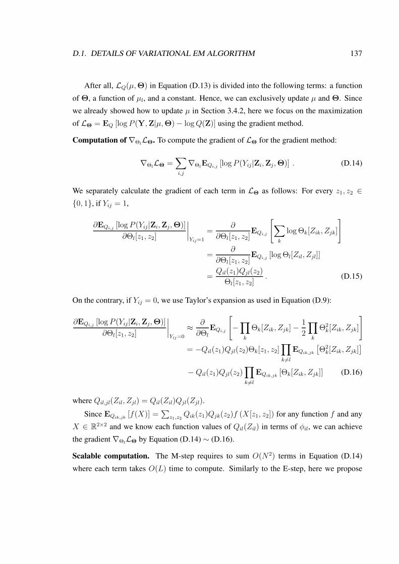
D.1. DETAILS OF VARIATIONAL EM ALGORITHM 137
After all, LQ(µ,Θ) in Equation (D.13) is divided into the following terms: a function
of Θ, a function of µl, and a constant. Hence, we can exclusively update µ and Θ. Since
we already showed how to update µ in Section 3.4.2, here we focus on the maximization
of LΘ = EQ [logP (Y,Z|µ,Θ)− logQ(Z)] using the gradient method.
Computation of∇ΘlLΘ. To compute the gradient of LΘ for the gradient method:
∇ΘlLΘ =
∑
i,j
∇ΘlEQi,j
[logP (Yij|Zi,Zj ,Θ)] . (D.14)
We separately calculate the gradient of each term in LΘ as follows: For every z1, z2 ∈0, 1, if Yij = 1,
∂EQi,j[logP (Yij|Zi,Zj ,Θ)]
∂Θl[z1, z2]
∣
∣
∣
∣
Yij=1
=∂
∂Θl[z1, z2]EQi,j
[
∑
k
log Θk[Zik, Zjk]
]
=∂
∂Θl[z1, z2]EQi,j
[log Θl[Zil, Zjl]]
=Qil(z1)Qjl(z2)
Θl[z1, z2]. (D.15)
On the contrary, if Yij = 0, we use Taylor’s expansion as used in Equation (D.9):
∂EQi,j[logP (Yij|Zi,Zj,Θ)]
∂Θl[z1, z2]
∣
∣
∣
∣
Yij=0
≈ ∂
∂Θl
EQi,j
[
−∏
k
Θk[Zik, Zjk]−1
2
∏
k
Θ2k[Zik, Zjk]
]
= −Qil(z1)Qjl(z2)Θk[z1, z2]∏
k 6=l
EQik,jk
[
Θ2k[Zik, Zjk]
]
−Qil(z1)Qjl(z2)∏
k 6=l
EQik,jk[Θk[Zik, Zjk]] (D.16)
where Qil,jl(Zil, Zjl) = Qil(Zil)Qjl(Zjl).
Since EQik,jk[f(X)] =
∑
z1,z2Qik(z1)Qjk(z2)f (X [z1, z2]) for any function f and any
X ∈ R2×2 and we know each function values of Qil(Zil) in terms of φil, we can achieve
the gradient ∇ΘlLΘ by Equation (D.14) ∼ (D.16).
Scalable computation. The M-step requires to sum O(N2) terms in Equation (D.14)
where each term takes O(L) time to compute. Similarly to the E-step, here we propose

138 APPENDIX D. DETAILS OF THE MAGFIT ALGORITHM
the scalable algorithm by separating Equation (D.14) into two parts, the fixed part for an
empty graph and the adjustment part for the actual edges:
∇ΘlLΘ =
∑
i,j
∇ΘlEQi,j
[logP (0|Zi,Zj ,Θ)]
+∑
Yij=1
∇ΘlEQi,j
[logP (1|Zi,Zj ,Θ)− logP (0|Zi,Zj ,Θ)] . (D.17)
We then approximate the first term in Equation (D.17) as follows:
∑
i,j
∇ΘlEQi,j
[logP (0|Zi,Zj ,Θ)] = ∇ΘlEQi,j
[
∑
i,j
logP (0|Zi,Zj ,Θ)
]
≈ ∇ΘlEQi,j
[N(N − 1)EZ[logP (0|Z,Θ)]]
= ∇ΘlN(N − 1)EZ[logP (0|Z,Θ)] . (D.18)
Since each Zil marginally follows the Bernoulli distribution with µl, Equation (D.18) is
computed by Equation (D.16) in O(L) time. As the second term in Equation (D.17) re-
quires only O(LE) time, the computation time of the M-step is finally reduced to O(LE)
time.

Bibliography
[1] E. M. Airoldi, D. M. Blei, S. E. Fienberg, and E. P. Xing. Mixed membership
stochastic blockmodels. Journal of Machine Learning Research, 9:1981–2014,
2008.
[2] R. Albert and A. L. Barabasi. Statistical mechanics of complex networks. Reviews
of Modern Physics, 74(1):47–97, 2002.
[3] R. Albert, H. Jeong, and A.-L. Barabasi. Diameter of the world-wide web. Nature,
401:130–131, 1999.
[4] L. Backstrom and J. Leskovec. Supervised random walks: Predicting and recom-
mending links in social networks. In WSDM ’11: Proceedings of the 4th ACM
International Conference on Web Search and Data Mining, 2011.
[5] A.-L. Barabasi and R. Albert. Emergence of scaling in random networks. Science,
286:509–512, 1999.
[6] P. S. Bearman, J. Jones, and J .R. Udry. The national longitudinal study of adolescent
health: Research design, 1997.
[7] D. M. Blei, A. Y. Ng, and M. I. Jordan. Latent dirichlet allocation. Journal of
Machine Learning Research, 3(4-5):993–1022, 2003.
[8] A. Blum, H. Chan, and M. Rwebangira. A random-surfer web-graph model. In
ANALCO ’06: Proceedings of the 3rd Workshop on Analytic Algorithmics and Com-
binatorics, 2006.
139

140 BIBLIOGRAPHY
[9] B. Bollobas. The diameter of random graphs. IEEE Transactions on Information
Theory, 36(2):285–288, 1990.
[10] B. Bollobas. 2001.
[11] A. Bonato, D. F. Gleich, M. Kim, D. Mitsche, P. Pralat, A. Tian, and S. J. Young.
Dimensionality of social networks using motifs and eigenvalues. arXiv:1405.0157,
2014.
[12] A. Bonato, N. Hadi, P. Horn, P. Prałat, and C. Wang. Models of online social net-
works. Internet Mathematics, 6(3):285–313, 2009.
[13] A. Bonato, J. Janssen, and P. Prałat. The geometric protean model for on-line social
networks. In WAW ’10: Proceedings of the 7th Workshop on Algorithms and Models
for the Web Graph, 2010.
[14] A. Broder, R. Kumar, F. Maghoul, P. Raghavan, S. Rajagopalan, R. Stata,
A. Tomkins, and J. Wiener. Graph structure in the web: experiments and mod-
els. In WWW ’00: Proceedings of the 9th International Conference on World Wide
Web, 2000.
[15] D. Chakrabarti, Y. Zhan, and C. Faloutsos. R-mat: A recursive model for graph
mining. In SDM ’04: Proceedings of the SIAM International Conference on Data
Mining, 2004.
[16] J. Chang and D. M. Blei. Relational topic models for document networks. In AIS-
TATS ’09: Proceedings of the 20th International Conference on Artificial Intelli-
gence and Statistics, 2009.
[17] F. R. K. Chung and L. Lu. The diameter of sparse random graphs. Advances in
Applied Mathematics, 26(4):257–279, 2001.
[18] Fan Chung and Linyuan Lu. Connected components in random graphs with given
expected degree sequences. Annals of Combinatorics, 6:125–145, 2002.

BIBLIOGRAPHY 141
[19] A. Clauset, C. R. Shalizi, and M. E. J. Newman. Power-law distributions in empirical
data. SIAM Review, 51(4):661–703, 2009.
[20] M. Craven, D. DiPasquo, D. Freitag, A. McCallum, T. Mitchell, K. Nigam, and
S. Slattery. Learning to extract symbolic knowledge from the world wide web. In
AAAI ’98: Proceedings of the 15th American Association for Articial Intelligence,
1998.
[21] D. J. de S. Price. A general theory of bibliometric and other cumulative advantage
processes. Journal of the American Society for Information Science, 27(5–6):292–
306, 1976.
[22] S. N. Dorogovtsev, A. V. Goltsev, and J. F. F. Mendes. Pseudofractal scale-free web.
Physical Review E, 65(6):066122, 2002.
[23] S. Duane, A.D. Kennedy, B. J. Pendleton, and D. Roweth. Hybrid monte carlo.
Physics Letter B, 195(2):216–222, 1987.
[24] David Easley and Jon Kleinberg. Cambridge, 2010.
[25] P. Erdos and A. Renyi. On the evolution of random graphs. Publication of the
Mathematical Institute of the Hungarian Academy of Science, 5:17–67, 1960.
[26] M. Faloutsos, P. Faloutsos, and C. Faloutsos. On power-law relationships of the
internet topology. In SIGCOMM ’99, pages 251–262, 1999.
[27] J. Foulds, A. U. Asuncion, C. DuBois, C. T. Butts, and P. Smyth. A dynamic rela-
tional infinite feature model for longitudinal social networks. In AISTATS ’11: Pro-
ceedings of the 14th International Conference on Artificial Intelligence and Statis-
tics, 2011.
[28] W. Fu, L. Song, and E. P. Xing. Dynamic mixed membership blockmodel for evolv-
ing networks. In ICML ’09: Proceedings of the 26th International Conference on
Machine Learning, 2009.

142 BIBLIOGRAPHY
[29] S. J. Gershman, P. I. Frazier, and D. M. Blei. Distance dependent infinite latent
feature models. arXiv:1110.5454, 2012.
[30] L. Getoor, E. Segal, B. Taskar, and D. Koller. Probabilistic models of text and link
structure for hypertext classification. In IJCAI Workshop on Text Learning: Beyond
Supervision, 2001.
[31] Z. Ghahramani and M. I. Jordan. Factorial hidden markov models. Machine Learn-
ing, 29(2-3):245–273, 1997.
[32] David F. Gleich and Art B. Owen. Moment based estimation of stochastic Kronecker
graph parameters. Internet Mathematics, 8(3):232–256, 2012.
[33] D.S. Goldberg and F.P. Roth. Assessing experimentally derived interactions in a
small world. Proceedings of the National Academy of Sciences, 100(8):4372, 2003.
[34] M. S. Granovetter. The strength of weak ties. volume 78, pages 1360–1380, 1973.
[35] T. L. Griffithsths and Z. Ghahramani. The indian buffet process: An introduction
and review. Journal of Machine Learning Research, 12(Apr):1185–1224, 2011.
[36] F. Guo, S. Hanneke, W. Fu, and E. P. Xing. Recovering temporally rewiring net-
works: a model-based approach. In ICML ’07: Proceedings of the 24th International
Conference on Machine Learning, 2007.
[37] G. J. Hahn and S. S. Shapiro. Statistical Models in Engineering, page 95. John
Wiley & Sons, Inc., 1994.
[38] S. Hanneke, W. Fu, and E. P. Xing. Discrete temporal models of social networks.
Electronic Journal of Statistics, 4:585–605, 2010.
[39] C. Heaukulani and Z. Ghahramani. Dynamic probabilistic models for latent feature
propagation in social networks. In ICML ’13: Proceedings of the 30th International
Conference on Machine Learning, 2013.

BIBLIOGRAPHY 143
[40] Q. Ho, L. Song, and E. P. Xing. Evolving cluster mixed-membership blockmodel
for time-varying networks. In AISTATS ’11: Proceedings of the 14th International
Conference on Artificial Intelligence and Statistics, 2011.
[41] P. Hoff, A. Raftery, and M. Handcock. Latent space approaches to social network
analysis. Journal of the American Statistical Association, 97:1090–1098, 2002.
[42] P. Holland, K. B. Laskey, and S. Leinhardt. Stochastic blockmodels: Some first
steps. Social Networks, 5:109–137, 1983.
[43] P. Holme. Core-periphery organization of complex networks. Physical Review E,
72:046111, 2005.
[44] K. Ishiguro, T. Iwata, N. Ueda, and J. Tenenbaum. Dynamic infinite relational model
for time-varying relational data analysis. In NIPS ’10: Advances in Neural Informa-
tion Processing Systems 23, 2010.
[45] S. Kairam, D. Wang, and J. Leskovec. The life and death of online groups: Pre-
dicting group growth and longevity. In WSDM ’12: Proceedings of the 5th ACM
International Conference on Web Search and Data Mining, 2012.
[46] B. Karrer and M. E. J. Newman. Stochastic blockmodels and community structure
in networks. Physical Review E, 83(1-2):016107, 2011.
[47] C. Kemp, J. B. Tenenbaum, T. L. Grifths, T. Yamada, and N. Ueda. Learning systems
of concepts with an innite relational model. In AAAI ’06: Proceedings of the 21st
American Association for Articial Intelligence, 2006.
[48] M. Kim and J. Leskovec. Modeling social networks with node attributes using the
multiplicative attribute graph model. In UAI ’11: Proceedings of the 27th Confer-
ence on Uncertainty in Articial Intelligence, 2011.
[49] M. Kim and J. Leskovec. Latent multi-group membership graph model. In ICML
’12: Proceedings of the 29th International Conference on Machine Learning, 2012.

144 BIBLIOGRAPHY
[50] M. Kim and J. Leskovec. Multiplicative attribute graph model of real-world net-
works. Internet Mathematics, 8(1-2):113–160, 2012.
[51] M. Kim and J. Leskovec. Nonparametric multi-group membership model for dy-
namic networks. In NIPS ’13: Advances in Neural Information Processing Systems
26, 2013.
[52] M. Kim, R. Sumbaly, and S. Shah. Root cause detection in a service-oriented archi-
tecture. In SIGMETRICS ’13: Proceedings of the ACM SIGMETRICS/international
conference on Measurement and modeling of computer systems, 2013.
[53] Myunghwan Kim and Jure Leskovec. Network completion problem: Inferring miss-
ing nodes and edges in networks. In SDM ’11: Proceedings of the SIAM Interna-
tional Conference on Data Mining, 2011.
[54] J. M. Kleinberg. Navigation in a small world. Nature, 406(6798), August 2000.
[55] J. M. Kleinberg, S. R. Kumar, P. Raghavan, S. Rajagopalan, and A. Tomkins. The
web as a graph: Measurements, models, and methods. In COCOON ’99: Proceed-
ings of the International Converence on Combinatorics and Computing, 1999.
[56] P. L. Krapivsky and S. Redner. Network growth by copying. Physical Review E,
71:036118, 2005.
[57] R. Kumar, P. Raghavan, S. Rajagopalan, D. Sivakumar, A. Tomkins, and E. Upfal.
Stochastic models for the web graph. In FOCS ’00: Proceedings of the 41st Annual
Symposium on Foundations of Computer Science, page 57, 2000.
[58] J. Leskovec, L. Backstrom, R. Kumar, and A. Tomkins. Microscopic evolution of
social networks. In KDD ’08: Proceedings of the 14th ACM SIGKDD International
Conference on Knowledge Discovery and Data Mining, pages 462–470, 2008.
[59] J. Leskovec, D. Chakrabarti, J. Kleinberg, C. Faloutsos, and Z. Ghahramani. Kro-
necker graphs: An approach to modeling networks. Journal of Machine Learning
Research, 11:985–1042, 2010.

BIBLIOGRAPHY 145
[60] J. Leskovec and C. Faloutsos. Scalable modeling of real graphs using kronecker
multiplication. In ICML ’07: Proceedings of the 24th International Conference on
Machine Learning, 2007.
[61] J. Leskovec and E. Horvitz. Planetary-scale views on a large instant-messaging
network. In WWW ’08: Proceedings of the 17th International Conference on World
Wide Web, 2008.
[62] J. Leskovec, D. Huttenlocher, and J. Kleinberg. Signed networks in social media. In
CHI ’10: Proceedings of ACM SIGCHI Conference on Human Factors in Computing
Systems, 2010.
[63] J. Leskovec, J. M. Kleinberg, and C. Faloutsos. Graphs over time: densification
laws, shrinking diameters and possible explanations. In KDD ’05: Proceedings
of the 11th ACM SIGKDD International Conference on Knowledge Discovery and
Data Mining, pages 177–187, 2005.
[64] J. Leskovec, K. J. Lang, A. Dasgupta, and M. W. Mahoney. Community structure in
large networks: Natural cluster sizes and the absence of large well-defined clusters.
Internet Mathematics, 6(1):29–123, 2009.
[65] D. Liben-Nowell and J. M. Kleinberg. The link prediction problem for social net-
works. In CIKM ’03: Proceedings of the 12th International Conference on Informa-
tion and Knowledge Management, 2003.
[66] D. Liben-Nowell, J. Novak, R. Kumar, P. Raghavan, and A. Tomkins. Geographic
routing in social networks. Proceedings of the National Academy of Sciences,
102(33):11623–11628, Aug 2005.
[67] J. R. Lloyd, P. Orbanz, Z. Ghahramani, and D. M. Roy. Random function priors for
exchangeable arrays with applications to graphs and relational data. In NIPS ’12:
Advances in Neural Information Processing Systems 25, 2012.
[68] L. Lu. The diameter of random massive graphs. In SODA ’01: Proceedings of the
12th annual ACM-SIAM Symposium on Discrete Algorithms, pages 912–921, 2001.

146 BIBLIOGRAPHY
[69] M. Mahdian and Y. Xu. Stochastic kronecker graphs. In WAW ’07: Proceedings of
the 5th Workshop on Algorithms and Models for the Web Graph, 2007.
[70] M. McGlohon, L. Akoglu, and C. Faloutsos. Weighted graphs and disconnected
components: patterns and a generator. In KDD ’08: Proceedings of the 14th
ACM SIGKDD International Conference on Knowledge Discovery and Data Min-
ing, 2008.
[71] M. McPherson. An ecology of affiliation. American Sociological Review,
48(4):519–532, 1983.
[72] M. McPherson and J. R. Ranger-Moore. Evolution on a dancing landscape: Organi-
zations and networks in dynamic blau space. Social Forces, 70(1):19–42, 1991.
[73] M. McPherson, L. Smith-Lovin, and J. M. Cook. Birds of a feather: Homophily in
social networks. Annual Review of Sociology, 27(1):415–444, 2001.
[74] S. Milgram. The small-world problem. Psychology Today, 2:60–67, 1967.
[75] K. T. Miller, T. L. Grifths, and M. I. Jordan. Nonparametric latent feature models for
link prediction. In NIPS ’09: Advances in Neural Information Processing Systems
22, 2009.
[76] M. Mørup, M. N. Schmidt, and L. K. Hansen. Infinite multiple membership rela-
tional modeling for complex networks. In IEEE International Workshop on Machine
Learning for Signal Processing, 2011.
[77] R. Nallapati, A. Ahmed, E. Xing, and W. W. Cohen. Joint latent topic models for
text and citations. In KDD ’08: Proceedings of the 14th ACM SIGKDD International
Conference on Knowledge Discovery and Data Mining, 2008.
[78] J. P. Onnela, J. Saramaki, J. Hyvonen, G. Szabo, D. Lazer, K. Kaski, J. Kertesz,
and A.-L. Barabasi. Structure and tie strengths in mobile communication networks.
Proceedings of the National Academy of Sciences, 104(18):7332–7336, 2007.

BIBLIOGRAPHY 147
[79] G. Palla, L. Lovasz, and T. Vicsek. Multifractal network generator. Proceedings of
the National Academy of Sciences, 107(17):7640–7645, 2010.
[80] K. Palla, D. A. Knowles, and Z. Ghahramani. An infinite latent attribute model for
network data. In ICML ’12: Proceedings of the 29th International Conference on
Machine Learning, 2012.
[81] I. Porteous, D. Newman, A. Ihler, A. Asuncion, P. Smyth, and M. Welling. Fast
collapsed gibbs sampling for latent dirichlet allocation. In KDD ’08: Proceedings
of the 14th ACM SIGKDD International Conference on Knowledge Discovery and
Data Mining, 2008.
[82] M. Radcliffe and S. Young. The spectra of multiplicative attribute graphs. preprint,
2012.
[83] S. Redner. How popular is your paper? an empirical study of the citation distribution.
European Physical Journal B, 4:131–134, 1998.
[84] E. M. Rogers and D. K. Bhowmik. Homophily-heterophily: Relational concepts for
communication research. The Public Opinion Quaterly, 34(4):523–538, 1970.
[85] S. Ross. A First Course in Probability. 7th edition.
[86] P. Sarkar, D. Chakrabarti, and M. I. Jordan. Nonparametric link prediction in dy-
namic networks. In ICML ’12: Proceedings of the 29th International Conference on
Machine Learning, 2012.
[87] P. Sarkar and A. W. Moore. Dynamic social network analysis using latent space
models. In NIPS ’05: Advances in Neural Information Processing Systems 18, 2005.
[88] J. Scott, R. Gass, J. Crowcroft, P. Hui, C. Diot, and A. Chaintreau. CRAWDAD data
set cambridge/haggle (v. 2009-05-29), May 2009.
[89] S. L. Scott. Bayesian methods for hidden markov models. Journal of the American
Statistical Association, 97(457):337–351, 2002.

148 BIBLIOGRAPHY
[90] P. Sen, G. Namata, M. Bilgic, L. Getoor, B. Gallagher, and T. Eliassi-rad. Collective
classification in network data. AI Magazine, 29(3), 2008.
[91] M. Seshadri, S. Machiraju, A. Sridharan, J. Bolot, C. Faloutsos, and J. Leskovec.
Mobile call graphs: Beyond power-law and lognormal distributions. In KDD ’08:
Proceedings of the 14th ACM SIGKDD International Conference on Knowledge Dis-
covery and Data Mining, 2008.
[92] M. Shiga, I. Takigawa, and H. Mamitsuka. Annotating gene function by combin-
ing expression data with a modular gene network. Bioinformatics, 23(13):i468–78,
2007.
[93] T. A. B. Snijders, G. G. van de Bunt, and C. E. G. Steglich. Introduction to stochastic
actor-based models for network dynamics. Social Networks, 32(1):44–60, 2010.
[94] T. A.B. Snijders, A. Lomi, and V. J. Torlo. A model for the multiplex dynamics of
two-mode and one-mode networks, with an application to employment preference,
friendship, and advice. Social Networks, 35(2):265–276, 2013.
[95] J. Tang, J. Zhang, L. Yao, J. Li, L. Zhang, and Z. Su. Arnetminer: Extraction
and mining of academic social networks. In KDD ’08: Proceedings of the 14th
ACM SIGKDD International Conference on Knowledge Discovery and Data Min-
ing, 2008.
[96] B. Taskar, M. F. Wong, P. Abbeel, and D. Koller. Link prediction in relational data.
In NIPS ’03: Advances in Neural Information Processing Systems 16, 2003.
[97] S. L Tauro, C. Palmer, G. Siganos, and M. Faloutsos. A simpe conceptual model fo
the internet topology. GLOBECOM ’01: Global Telecommunications Conference,
3:1667–1671, 2001.
[98] A. L. Traud, P. J. Mucha, and M. A. Porter. Social structure of facebook networks.
arXiv:1102.2166v1, 2011.

BIBLIOGRAPHY 149
[99] Charalampos E. Tsourakakis. Fast counting of triangles in large real networks with-
out counting: Algorithms and laws. In ICDM ’08: Proceedings of IEEE Interna-
tional Conference on Data Mining, 2008.
[100] J. van Gael, Y. W. Teh, , and Z. Ghahramani. The infinite factorial hidden markov
model. In NIPS ’09: Advances in Neural Information Processing Systems 22, 2009.
[101] A. Vazquez. Disordered networks generated by recursive searches. Europhysics
Letters, 54(4):430–435, 2001.
[102] Y. J. Wang and G. Y. Wong. Stochastic blockmodels for directed graphs. Journal of
the American Statistical Association, 82(397):8–19, 1987.
[103] S. Wasserman and P. Pattison. Logit models and logistic regressions for social net-
works. Psychometrika, 60:401–425, 1996.
[104] D. J. Watts and S. H. Strogatz. Collective dynamics of ’small-world’ networks.
Nature, 393:440–442, 1998.
[105] R. Xiang, J. Neville, and M. Rogati. Modeling relationship strength in online social
networks. In WWW ’10: Proceedings of the 19th international conference on World
wide web, 2010.
[106] Z. Xu, V. Tresp, K. Yu, and H.-P. Kriegel. Innite hidden relational models. In UAI
’06: Proceedings of the 22nd Conference on Uncertainty in Articial Intelligence,
2006.
[107] J. Yang and J. Leskovec. Community-affiliation graph model for overlapping com-
munity detection. In ICDM ’13: Proceedings of IEEE International Conference on
Data Mining, 2012.
[108] J. Yang, J. McAuley, and J. Leskovec. Community detection in networks with node
attributes. In ICDM ’13: Proceedings of IEEE International Conference on Data
Mining, 2013.

150 BIBLIOGRAPHY
[109] S. J. Young and E. R. Scheinerman. Random Dot Product Graph Models for Social
Networks, volume 4863 of Lecture Notes in Computer Science. Springer Berlin,
2007.