1

Modeling Mobile Edge Computing Deployments forLow Latency Multimedia Services

Jorge Martın-Perez*†, Luca Cominardi†, Carlos J. Bernardos†, Antonio de la Oliva†, Arturo Azcorra†‡†Universidad Carlos III de Madrid, Spain

‡IMDEA Networks Institute, Spain

Abstract—Multi-access Edge Computing (MEC) technologiesbring important improvements in terms of network bandwidth,latency and use of context information, critical for services likemultimedia streaming, augmented and virtual reality. In futuredeployments, operators will need to decide how many MECPoints of Presence (PoPs) are needed and where to deploy them,also considering the number of base stations needed to supportthe expected traffic. This article presents an application ofinhomogeneous Poisson point processes with hard-core repulsionto model feasible MEC infrastructure deployments. With thepresented methodology a mobile network operator knows whereto locate the MEC PoPs and associated base stations to supporta given set of services. We evaluate our model with simulationsin realistic scenarios, namely Madrid city center, an industrialarea, and a rural area.

Index Terms—5G, MEC, Point Process, Deployment, Charac-terization, Network Slicing, Streaming, Low Latency, AugmentedReality, Virtual Reality.

I. INTRODUCTION

The next generation of mobile networks, the so-called 5G,comes with the promise of new and enhanced services, throughthe introduction of an improved radio interface, plus a networkcore that allows to dynamically deploy services closer to thelocation of the users. 5G networks will need to accommodateon top of the same physical infrastructure multiple kinds ofservices with very distinct requirements, spanning from ultra-low latency to high bandwidth and high reliability. Theseservices are grouped in three main categories by 3GPP:enhanced Mobile Broadband (eMBB), Ultra-Reliable and LowLatency Communications (URLLC), and Massive Internet ofThings (MIoT) [1].

Among the several use cases that may be supported by5G are Augmented Reality (AR) and Virtual Reality (VR),which can be included into eMBB and URLLC categories. Inparticular, AR/VR impose a Motion to Photon (MTP) latencythat does not exceed 20 ms, requiring a network Round TripTime (RTT) below 2 ms [2]. Moreover, a response within1 ms is desired in case of visual-haptic interaction [3]. Al-though the new 5G radio interface promises ultra low latencyenhancements, to truly fulfill the VR/AR ultra-low latencyrequirements it is also necessary to reduce the communication

*Corresponding author: jmartinp@it.uc3m.esParts of this paper have been published in the Proceedings of the IEEE BMSB2018, Valencia, SpainWork partially funded by the EU H2020 5G-CORAL Project (grant no.761586) and by the EU H2020 5G-TRANSFORMER Project (grant no.761536).

Mobile edge host / MEC PoP

Mobile edgeplatform

Virtualization infrastructure

MEapp

MEapp

MEapp

Service Mobile edgeplatform manager

Mobile edgeorchestrator

Virtual infrastructure manager

Operations Support System

Fig. 1: ETSI MEC architecture.

distance by bringing the multimedia applications close to theend users. This is achieved by Multi-access (Mobile) EdgeComputing (MEC) [4] [5].

MEC is a key enabler for 5G technology and its mainprinciple is to host computation and storage at edge hosts,close to end users. Typically, these edge hosts are highlydistributed in the network, located close to the radio accessnetwork nodes (e.g., gNodeBs in 5G). As a result, MEC en-ables two types of services: (i) low-latency services, requiringa very low and bounded delay between the end user deviceand the server hosting the application; and, (ii) context-awareservices, which need to access end-user contexts, such as theuser channel quality conditions, in order to adapt the deliveredservice. MEC is being standardized within ETSI, via the MECISG group. A simplified version of the MEC architecturedefined by ETSI is shown in Fig. 1. The main componentsof the architecture include: the Mobile Edge (ME) host, theME application and the MEO (ME orchestrator). The MEChost is the key element. It provides the environment to runME applications, while it interacts with the mobile networkentities, via the Mobile Edge Platform (MEP), to provide MEservices and deliver mobile traffic to MEC applications.

ME hosts are expected to be deployed by mobile operatorsin their 5G network infrastructure. To enable the pervasiveservice offering of AR/VR multimedia services, it is hencenecessary to study how a MEC deployment should look liketo support URLLC. Specifically, it is important to understandwhat are the suitable locations of future MEC Points ofPresence (PoP) within the mobile network infrastructure. Asa result, in this article we develop a novel model for MEC

2

scenario deployments, analyzing how many MEC Points ofPresence (PoP) are needed to meet a given set of requirements.

This work has been done within the framework of the 5G-TRANSFORMER project. The 5G-TRANSFORMER maingoal is to support vertical industries (particularly focusingon low latency) through flexible slicing and federation ofresources across multiple domains. This article is structuredas follows: Section II introduces related work, Section IIIpresents in detail our model, which is then applied to a realisticscenario in Section IV and validated in Section V. Finally,Section VI concludes this article with some final remarks andhints for future work.

II. RELATED WORK

Existing work in the literature, such as [6], studies feasi-ble network infrastructure deployments using Point Processes(PPs) that randomly scatter points on some space (e.g., a line,a Cartesian plane, etc.). In particular [6] uses Poisson PPs(PPPs), a family of PPs used to generate the location of basestations (BSs) that are distributed following Poisson countingprocesses. PPPs can impose a minimum distance between BSsto increase coverage area and reduce the interference (seehard-core PPPs in [7]), and control if every region in thespace has the same or different probability to host a BS (seehomogeneous and inhomogeneous PPPs, respectively, in [7]).

Different types of PPPs are used in the State of the Art(SoA). For instance, the authors of [8] use Neyman-Scott [9]PPPs to generate small base stations (BSs) clustered aroundmacro BSs with the objective of modeling the coverage andinterference in heterogeneous networks. Similarly, [10] showsthat homogeneous PPPs can be used in realistic deploymentscenarios to reduce interference and increase the coverage areaby properly configuring the distance between the BS sites andthe intensity parameter.

Works like [6] and [11] analyze potential infrastructuredeployments with the help of homogeneous PPPs. The for-mer focuses on studying the cost of a Cloud Radio AccessNetwork (Cloud-RAN) infrastructure using PPPs, while thelatter analyzes the throughput and coverage of end users, usingPPPs to determine hotspot locations in heterogeneous cellularnetworks.

Regarding future MEC deployments in real scenarios,[12] studies the existing BS deployment in several USAlocations (including highways and rural areas). Likewise, [13]characterizes AR/VR deployments in stadium scenarios in theperspective of forthcoming Tokyo 2020 Olympics. The authorsconclude that such use case requires a single media roomdedicated to the video processing and proposes two distinctBS deployments: one powerful BS in the stadium (e.g., on theroof) or multiple small BSs (e.g., located close to the stadiumvomitoria1).

The work presented in this article studies the deploymentof MEC PoPs in real urban, industrial and rural scenarios tosatisfy the 5G slices requirements, including the most stringentlatency expected by the 5G AR/VR applications (as donein [13]).

1A vomitorium is a passage situated below a tier of seats in a stadium.

Unlike [12], this paper accounts for 5G New Radio (NR)technologies rather than legacy radio technologies. We gener-ate feasible locations for gNodeBs, and derive deployments ofMEC PoPs guaranteeing low latency requirements that deploy-ments in [12] do not ensure. We use inhomogeneous MaternII PPs (see Proposition III.2 in Sec. III-A for more details) toobtain feasible locations for the BSs. The inhomogeneity ofthese processes improves the Matern PPs in the SoA by locat-ing the BSs based on the density of population. That is, moreBSs are generated where the population density2 is higher. Inother words, the inhomogeneity allows to concentrate the BSswhere they are really needed and to minimize the generationin those areas with little traffic demand.

The generated BS locations are used next to derive therequired number of PoPs and their potential location.

III. MODEL

This section presents the model used to both generatethe BSs of future MEC deployments, and to determine thelocations of the MEC PoPs to which the BSs are assigned.In our model a BS is the first connection point in the RANaccessed by the User Equipment (UE), for example a 2GBS, a 3G NodeB, a 4G eNodeB, or a 5G gNodeB. InSec. III-A we extend Matern PPs to introduce inhomogeneityand generate BSs based on the population density. The derivedprocesses, namely inhomogeneous Matern I and II PPs, imposea minimum distance between BSs to obtain a better coverage.Moreover, we show that Matern II PPs are more suitable forBSs generation because of their relaxed thinning procedure.Sec. III-B presents the algorithm used to generate MEC PoPsthat can satisfy imposed latency constraints among all the BSsthat are assigned to them.

A. Macro cells generation

With the model we aim to generate more BSs in regionswhere the population is higher. Here we refer to a regionR as a subset of a complete separable metric space R, forexample a map of Spain. Hence R can represent a city likeMadrid and the model locates BSs in city areas where thereare more people. To achieve this we consider that every regionR contains population circles Ci ⊂ R defined by a center ciand a revolution function fi(x) (with i ∈ [1, RC ]∩N, and RCthe number of population circles defined inside the region R).

The revolution function fi(x) with x ∈ Ci determines whereit is more likely to have a person in Ci. This function leadsto a surface of revolution defined at Ci that can be expressedas fi(‖x − ci‖d), and which height expresses the amount ofpeople at a given location x ∈ R. Therefore, the presence ofpeople at x ∈ R is expressed as:

G(x) :=∑i

fi(‖x− ci‖d), ∀Ci ⊂ R, ∀d ∈ N (1)

where G(x) is referred as gentrification in the followingparagraphs.

2In our scenarios we refer to human population. Nevertheless, inhomoge-neous Matern PPs can be applied to other types of populations.

3

f1 f2

C1 C2

G(x)

R

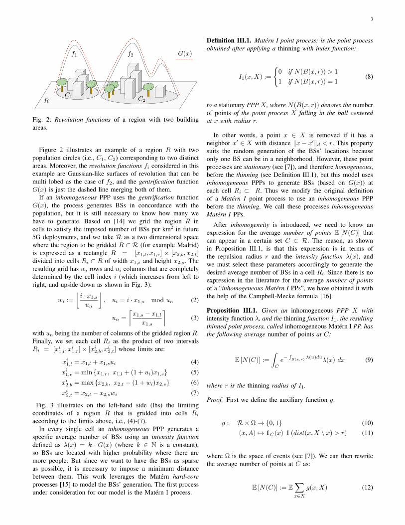
Fig. 2: Revolution functions of a region with two buildingareas.

Figure 2 illustrates an example of a region R with twopopulation circles (i.e., C1, C2) corresponding to two distinctareas. Moreover, the revolution functions fi considered in thisexample are Gaussian-like surfaces of revolution that can bemulti lobed as the case of f2, and the gentrification functionG(x) is just the dashed line merging both of them.

If an inhomogeneous PPP uses the gentrification functionG(x), the process generates BSs in concordance with thepopulation, but it is still necessary to know how many wehave to generate. Based on [14] we grid the region R incells to satisfy the imposed number of BSs per km2 in future5G deployments, and we take R as a two dimensional spacewhere the region to be gridded R ⊂ R (for example Madrid)is expressed as a rectangle R = [x1,l, x1,r] × [x2,b, x2,t]divided into cells Ri ⊂ R of width x1,s and height x2,s. Theresulting grid has wi rows and ui columns that are completelydetermined by the cell index i (which increases from left toright, and upside down as shown in Fig. 3):

wi :=

⌊i · x1,s

un

⌋, ui = i · x1,s mod un (2)

un =

⌈x1,s − x1,l

x1,s

⌉(3)

with un being the number of columns of the gridded region R.Finally, we set each cell Ri as the product of two intervalsRi = [xi1,l, x

i1,r]× [xi2,b, x

i2,t] whose limits are:

xi1,l = x1,l + x1,sui (4)

xi1,r = min x1,r, x1,l + (1 + ui)x1,s (5)

xi2,b = max x2,b, x2,t − (1 + wi)x2,s (6)

xi2,t = x2,t − x2,swi (7)

Fig. 3 illustrates on the left-hand side (lhs) the limitingcoordinates of a region R that is gridded into cells Riaccording to the limits above, i.e., (4)-(7).

In every single cell an inhomogeneous PPP generates aspecific average number of BSs using an intensity functiondefined as λ(x) = k · G(x) (where k ∈ N is a constant),so BSs are located with higher probability where there aremore people. But since we want to have the BSs as sparseas possible, it is necessary to impose a minimum distancebetween them. This work leverages the Matern hard-coreprocesses [15] to model the BSs’ generation. The first processunder consideration for our model is the Matern I process.

Definition III.1. Matern I point process: is the point processobtained after applying a thinning with index function:

I1(x,X) :=

0 if N(B(x, r)) > 1

1 if N(B(x, r)) = 1(8)

to a stationary PPP X , where N(B(x, r)) denotes the numberof points of the point process X falling in the ball centeredat x with radius r.

In other words, a point x ∈ X is removed if it has aneighbor x′ ∈ X with distance ‖x− x′‖d < r. This propertysuits the random generation of the BSs’ locations becauseonly one BS can be in a neighborhood. However, these pointprocesses are stationary (see [7]), and therefore homogeneous,before the thinning (see Definition III.1), but this model usesinhomogeneous PPPs to generate BSs (based on G(x)) ateach cell Ri ⊂ R. Thus we modify the original definitionof a Matern I point process to use an inhomogeneous PPPbefore the thinning. We call these processes inhomogeneousMatern I PPs.

After inhomogeneity is introduced, we need to know anexpression for the average number of points E [N(C)] thatcan appear in a certain set C ⊂ R. The reason, as shownin Proposition III.1, is that this expression is in terms ofthe repulsion radius r and the intensity function λ(x), andwe must select these parameters accordingly to generate thedesired average number of BSs in a cell Ri. Since there is noexpression in the literature for the average number of pointsof a “inhomogeneous Matern I PPs”, we have obtained it withthe help of the Campbell-Mecke formula [16].

Proposition III.1. Given an inhomogeneous PPP X withintensity function λ, and the thinning function I1, the resultingthinned point process, called inhomogeneous Matern I PP, hasthe following average number of points at C:

E [N(C)] :=

∫C

e−∫B(x,r)

λ(u)duλ(x) dx (9)

where r is the thinning radius of I1.

Proof. First we define the auxiliary function g:

g : R× Ω→ 0, 1 (10)(x,A) 7→ 1C(x) 1 (dist(x,X \ x) > r) (11)

where Ω is the space of events (see [7]). We can then rewritethe average number of points at C as:

E [N(C)] := E∑x∈X

g(x,X) (12)

4

R0 R1 R2 R3 R4

R5 R6 R7 R8 R9

R10 R11 R12 R13 R14

R15 R16 R17 R18 R19

R20 R21 R22 R23 R24

R2

(x1,l, x2,t)

(x1,r, x2,b)x1,s

x2,s

R R2

(x21,r, x

22,b)

r

∇λ

Fig. 3: Gridded region on the left side, and macro cell generation inside a cell on the right side. Gray crosses without a celltower represent BS points that did not survive after the I2 thinning. The rhs shows how the region cell R2 is gridded whenthe repulsion radius is chosen as specified in Eq. (25) with N(R2) = 5.

Next, we use the Campbell-Mecke formula to obtain:

E∑x∈X

g(x,X) :=

∫REx[g(x,X)]λ(x) dx = (13)

=

∫R

∫Ω

g(x,X)Px(A) dA λ(x) dx = (14)

=

∫C

∫Ω

1 (dist(x,X \ x) > r)Px(A) dA λ(x) dx = (15)

=

∫C

Px (dist(x,X \ x) > r) λ(x) dx = (16)

=

∫C

P (N (B(x, r)) = 0) λ(x) dx (17)

where Px denotes the Palm probability. Finally, we apply thecapacity functional (see [7]) of a PPP to obtain the statedequality.

One drawback of these “inhomogeneous Matern I” pro-cesses is their very restrictive dependent thinning procedure,which might reach the case where all the points are re-moved in certain neighborhoods. To overcome such limitation,our model considers a second type of processes, known asMatern II point processes, that rely on marked point processes(see [7]). Matern II processes assign a mark to every pointgenerated so as to allow the dependent thinning processes(see [7]) distinguish which point is retained in a neighborhood.

Definition III.2. Matern II point process: is the point processobtained after applying a thinning with index function:

I2(x,m,X,MX) :=

1 if m = minm′∈MX

(x′,m′) :

x′ ∈ B(x, r)

0 otherwise(18)

to a stationary marked PPP X , where MX denote the marksassociated to the point process X .

In other words, among all the points falling in the ball ofradius r, only the one with the lowest mark m survives. Thesekind of processes present the advantage that even when theintensity function takes high values, at least one point remainsin every neighborhood. In our model this means that in acertain neighborhood there is no more than one BS.

If rather than using a stationary PPP before applyingthe dependent thinning I2, we use an inhomogeneous PPP(something novel in the SoA); then it is possible that theretained BS in a neighborhood is the one with higher λ(x) bychoosing the mark (x,m) as m ∼ 1

λ(x) . But still is missinghow we can control that a correct number of BSs is generatedat each region Ri ⊂ R based on the repulsion radius r andthe intensity function λ(x). Thus we proceed as with the“inhomogeneous Matern I” PPs to obtain an expression forthe average number of points (something novel in the SoA).

Proposition III.2. Given an inhomogeneous marked PPP Xwith intensity function λ, the thinning function I2, and marksm ∼ 1

λ(x) , the resulting thinned point process, called inhomo-geneous Matern II PP, has the following average number ofpoints at C:

E [N(C)] :=

∫C

e−∫B(x,r)

1(λ(u)>λ(x))λ(u)duλ(x) dx (19)

where r is the thinning radius of I2.

Proof. As in the proof of Proposition III.1, we proceed defin-ing the function g:

g : R× Ω→ 0, 1 (20)

(x,A) 7→ 1C(x) 1

(λ(x) = max

x′∈X∩B(x,r)λ(x′)

)(21)

Then, the average number of points in a subset C can beexpressed as in Eq. (12). Next, we apply the Campbell-Mecke

5

formula as in the previous proof and we obtain the averagenumber of points as:

E∑x∈X

g(x,X) :=

∫C

Px(λ(x) = max

x′∈X∩B(x,r)

)λ(x) dx =

(22)

=

∫C

P(N(B>λ(x)(x, r)

)= 0)λ(x) dx = (23)

=

∫C

e−∫B(x,r)

1(λ(u)>λ(x))λ(u)duλ(x) dx (24)

where B>λ(x)(x, r) = u : x ∈ B(x, r) ∧ λ(u) > λ(x) .

The right-hand side (rhs) of Fig. 3 depicts how to obtainBSs’ locations using an inhomogeneous Matern II PP (whoseaverage number of points is derived in Proposition III.2).First, it generates the gray crosses using an inhomogeneousPPP with intensity function λ(x) (note that more points aregenerated on the upper right corner because of the direction of∇λ(x)). Then, a I2 thinning is applied using repulsion radiusr with marks m ∼ 1

λ(x) , so only the gray cross with the mosttop-right coordinate falling within a ball of radius r survive.This surviving cross is hence illustrated as a cell tower inFig. 3.

As both Propositions III.1 and III.2 state, the averagenumber of points of “inhomogeneous Matern I and II” PPsdepend on the repulsion radius r. Then for a cell Ri ⊂ R, weneed to know which r allows the generation of the requirednumber of BSs. To generate N(Ri) points we set the cellrepulsion radius as:

r :=2√x1,s · x2,s

d√N(Ri)e

(25)

which grids Ri in cells that can contain the repulsion ballsB(x, r) of the Matern PPs. These new cells are squares ofside 2r and area 4r2 > πr2 = |B(x, r)|, and they divide theparent cell Ri in d

√N(Ri)e2 smaller cells that can host a

whole macro cell repulsion area.

B. MEC PoPs’ deployment

We assign the traffic of every BS generated in Sec. III-A toa MEC PoP that is deployed somewhere within the operators’network infrastructure, and at a specific geographic location(i.e., to minimize RTT). The further the distance between theMEC PoP at location m, and a BS at location x, the higher thepropagation delay l(·) of the link connecting them. The othertwo contributions for the packet Round Trip Time (RTT) arethe radio transmission delay tr between a BS and the finaluser, and the packet processing delay p(·):

RTT := 2l (‖x−m‖d) + 2p(M) + tr (26)

with p(M) denoting the processing delay introduced by thenetwork hops to be traversed to reach the network ring M .Hence, our model envisions the operator infrastructure as ahierarchy of network ringsM, in which traffic traverses morehops to reach network rings that are higher in the hierarchy(see Fig. 4). That is, taking ≺ as a relationship expressingwhich network ring is higher in the network hierarchy M, if

Ma,Mb ∈ M and Ma ≺ Mb, we can say that a MEC PoPdeployed at Ma is reached in less hops than one at Mb. Thus,p(Ma) < p(Mb), and network ring Ma aggregates less trafficthan Mb.

So if we place a MEC PoP at location m and assign it tonetwork ring M , after fixing the maximum RTT and radiotechnology, from Eq. (26) we know the maximum distance tothose BSs whose traffic is assigned to the new MEC PoP

‖x−m‖d ≤ l−1

(RTT − 2p(M)− tr

2

)= mM (27)

Algorithm 1 determines the MEC PoPs’ deployment in threestages:1) Initialization: the first stage (lines 1-4) creates the set of

MEC PoPs locations, the set of their network rings, theset of BSs and one matrix of locations x ∈ R per networkring. Each entry x in the matrix matrices[M ] representsthe number of BSs that can be assigned to a MEC PoPdeployed at a given location x and associated to the ringM ∈M

2) Candidates search: this second stage (lines 5-10) deter-mines how many BSs can be assigned to a MEC PoPdepending on its location and associated network ringM ∈ M. For every M it loops through each BS andincreases by one those location entries of matrices[M ]satisfying that if a MEC PoP is deployed there, it couldsatisfy the RTT and hence, the BS could be assigned tothat MEC PoP. If matrices[Ma][x0] = 4 after this stage,it would mean that a MEC PoP associated to Ma anddeployed at x0 would have 4 BSs assigned to itself.

3) MEC PoPs selection: this third and last stage (lines 11-35)is the main loop of Algorithm 1, and each iteration decidesa new MEC PoP location and network ring. It comprisestwo phases:

a) MEC PoP location: this phase (lines 15-24) obtainsthe best location where a MEC PoP can be located.It iterates through all the possible network rings in Msearching for the location where the maximum amountof BSs can be assigned to a MEC PoP. In case ofhaving multiple locations assigning the same amount ofBSs at different rings, let’s call them Ma,Mb, then thealgorithm selects the location related to the ring with theminimum propagation delay, i.e., min p(Ma), p(Mb).

b) Assignment update: the MEC PoP obtained in theprevious step handles the traffic of up to maximumnumber of BSs ringMaxBSs(), depending on the networkring where it is associated. Taking into account thatconsideration, this phase (lines 28-34) iterates throughevery BS assigned to the MEC PoP and updates everymatrices[M ] to reflect the assignment by decreasingin one unit the neighborhood of each BS. That is,if the new MEC PoP has an assigned BS at loca-tion x, the neighboring locations of x at every ring,i.e., matrices[M ][B(x,mM )], must be decreased byone. Thus if another MEC PoP is latter located in-side B(x,mM ), it knows that it will cover one lessBS. Finally all the assigned BSs are removed from theunassigned list.

6

Hence, Algorithm 1 iterates through every MEC PoP candidatelocation m, and chooses the one maximizing the number ofBSs falling inside the ball B(m,mM ). This process minimizesthe number of MEC PoPs, and is done for every possiblenetwork ring M to find the best (m,M) combination.

Data: BSs, R, RTTResult: MECPoPLocations, MECPoPRings

1 matrices = array(int.matrix(R), length = |M|);2 unassigned = Set(BSs);3 MECPoPLocations = Set();4 MECPoPRings = Set();5 foreach x in BSs do6 foreach M in M do7 mM = l−1

(RTT−2p(M)−tr

2

);

8 matrices[M ][B(x,mM )] += 1;9 end

10 end11 while not empty unassigned do12 covBSs = −1;13 MECPoP = NULL;14 ring = NULL;15 foreach M ∈M do16 maxCov = maxx′ matrices[M ][x′];17 moreBSsCovered = maxCov < covBSs;18 eQ = (maxCov = covBSs ∧ p(M) < p(ring));19 if moreBSsCovered OR eQ then20 covBSs = maxCov;21 MECPoP = x : matrices[M ][x] = maxCov;22 ring = M ;23 end24 end25 MECPoPLocations.add(MECPoP);26 MECPoPRings.add(ring);

27 ringMaxDis = l−1(RTT−2p(ring)−tr

2

);

28 assignBSs = BSs ∩ B(MECPoP, ringMaxDis);29 foreach x ∈ assignBSs.subset(ringMaxBSs(ring)) do30 foreach M ∈M do31 matrices[M ][B(x,mM )] -=1;32 end33 unassigned.pop(x);34 end35 end

Algorithm 1: MEC PoPs placement.

IV. APPLYING THE MODEL TO A REALISTIC SCENARIO

This section provides an example of applying the modeldescribed in Sec. III. Specifically, Sec. IV-A characterize thenetwork traffic and infrastructure to derive realistic valuesfor the average number of BSs/km2 and network RTT. Then,Section IV-B characterizes three deployment areas in Spain,namely Madrid city center (104 km2), Cobo Calleja industrialestate (8 km2), and Hoces del Cabriel valley (2193 km2);where the proposed model is applied.

TABLE I: Exemplary 5G traffic requirements.

SLICE FLOW REQUIREMENTS

Indoor Hotspot Up to 1Gbps/usereMBB Broadcast services Up to 200 Mbps/TV channel

High-speed vehicle Up to 100 Gbps/Km2

Discrete automation Maximum jitter of 1 µsURLLC Intelligent transport Reliability of 99.9999%

Tactile interaction Maximum latency of 0.5 ms1

MIoT Sensors data Up to 200 Mbps/Km2

1 Note: end-to-end maximum delay as defined in [18].

A. Characterization of network traffic and infrastructure

According to the Next Generation Mobile Network Alliance(NGMN) [17], 5G services are expected to be provided viaad-hoc network slices over the same physical infrastructure.In order to enable the desired traffic treatment in the networkinfrastructure, the 3rd Generation Private Partnership (3GPP)has defined a set of flows with the corresponding trafficrequirements for the eMBB and URLLC slices [18], whileNGMN in [19] defined the traffic requirements for the MIoTslice. eMBB services are characterized by high bandwidth andspan from classical mobile traffic (e.g., mobile terminals),to broadcast-like services (e.g., IPTV), high-speed vehicles(e.g., in-vehicle infotainment), indoor hotspot (e.g., fiber-likeaccess), and dense urban (e.g., crows in a stadium, square). Onthe contrary, URLLC services are characterized by low latencyand span from discrete automation (i.e., remote-controlledrobots), to intelligent transport systems (e.g., autonomouscars), and tactile interaction (e.g., augmented reality). Finally,MIoT services are characterized by a high number of inter-mittent and low-power communications (e.g., sensors). Table Ireports a selected number of the above traffic requirements asreported in [18], [19].

Based on the different slices and traffic flows introducedabove, the authors in [14] first identify three reference de-ployment scenarios, namely urban, industrial, and rural. Next,they characterize the average number of BSs/km2 for eachscenario. Specifically, they report for the urban scenario anaverage number of 72 BS/km2 in case of supporting the indoorhotspot traffic flow, which is characteristic of business districtsand office areas that require 4 BSs per building floor. Inresidential/commercial areas instead, the average number ofBS/km2 is 12 in urban scenarios. Similarly, 12 BSs are alsorequired in the industrial scenario to satisfy the traffic demandof 1 km2. Finally, the rural scenario considers a 4-lane road(e.g., highway) supporting the intelligent transport system flow(e.g., V2X) and requires 1 BS per kilometer of road.

The next step is to characterize the network infrastructure.To that end, we leverage the reference network infrastructureillustrated in [14] and based on [20]. The network infrastruc-ture comprises three segments: (i) access, (ii) aggregation, and(iii) core. The access comprises 6 BSs for each node M1connected via a point-to-point link, and 6 nodes M1 connectedin a ring topology. Thus, each access ring hence connects atotal of 36 BSs. It is worth highlighting that from a network

7

M1

Base Station

6x Base Stations per M1 node

6x M1 nodes per access ring

M2

4x access rings per M2 node

Access ring Aggregation ring

M3

6x M2 nodes per aggregation ring

2x aggregation rings per M3 node

M4

CoreAccess Aggregation

InternetCore ring

Fig. 4: Reference network infrastructure as illustrated in [14] and based on [20]

topology point of view, there is no difference whether the BSsare macro, micro, pico, and any variation thereof. For the sakeof validating our model, what really matters is the number ofBSs and how they are connected to the transport network.

Next, each aggregation ring comprises 6 M2 nodes, each ofwhich serves 4 access rings. In turn, each aggregation ring isserved by two M3 nodes for redundancy reasons, while eachM3 node provides gateway capabilities to 2 aggregation rings.Finally, M4 nodes are connected to the core ring and serveas gateway to M3 nodes. According to the reference networkinfrastructure, any of these BSs and M nodes (e.g., M1, M2,M3, and M4) is a good candidate for placing a MEC PoP.

To better understanding which location is most suitable, weneed to characterize the RTT. To that end, all the networklinks are assumed to be fiber optic and are characterized bya propagation delay of 5 µs/km [21]. We also consider aprocessing delay of 50 µs on each of the M nodes [22], [23].Therefore, the Eq. (26) becomes:

RTT = 2d · 5 µskm

+ 2M · 50µs+ UL+DL (28)

where d stands for the distance in kilometers between theMEC PoP and the BS, and M is the number of M nodes(i.e., number of hops) being traversed. For instance, M = 0in case of collocating the MEC PoP with the BSs, M = 1 incase of collocating the MEC PoP with M1 nodes, M = 2in case of collocating the MEC PoP with M2 nodes, etc.Therefore, the first two terms in the right hand side of Eq.(28) correspond to the propagation delay RTT and the packetprocessing delay RTT in the transport network, respectively.The last two terms (i.e., UL and DL) correspond instead tothe Uplink and Downlink delay over the radio link.

3GPP defines multiple profiles for the radio interface (i.e.,New Radio – NR) and each of these profiles is characterizedby distinct UL and DL delay values [24]. Bound to the moststringent one-way latency of 0.5 ms for the tactile interactionURLLC traffic flow (see Table I), the BSs used for the resultsexposed in Sec.V are 5G gNodeBs with the suitable radioprofiles that satisfy UL + DL < RTT = 1ms; hence “BS”refers to a 5G gNodeB from now on. Table II reports theNR profiles used, which all adopt an uplink semi-persistentscheduling (SPS), and the maximum distances d from a BS toa MEC PoP.

TABLE II: NR profiles satisfying the tactile interaction latency

PROFILE DL UL M1DISTANCE

M2DISTANCE

FDD 30 kHz 2s 0.39 ms 0.39 ms 12 km 2 km

FDD 120 kHZ 7s 0.33 ms 0.33 ms 24 km 14 km

TDD 120 kHz 7s 0.39 ms 0.39 ms 12 km 2 km

Note: FDD 30 kHz 2s stands for Frequency Division Duplex scheme witha subcarrier of 30 kHz and 2 symbols.Note: DL and UL values are the worst case transmission latenciespresented in [24].

B. Characterization of the deployment areas

Based on the identified urban, industrial, and rural scenarios,we select three reference areas in Spain to apply our model(see Sec. III) and obtain the MEC PoP locations. Specifically,we select Madrid city center for the urban scenario, CoboCalleja area for the industrial scenario, and Hoces del Cabrielvalley for the rural scenario; then we consider the followingcharacterization aspects.

1) Characterization of G(x): before applying the modelwe characterize each scenario’s gentrification function G(x),revolution function fi, and population circles Ci. Particularlyfi is based on the smoothstep function, which is derived fromHermite interpolation polynomials [25] and has the followingexpression:

SN (x) =

0 x ≤ 0

xN+1∑Nn=0

(N+nn

)(2N+1N−n

)(−x)n if 0 ≤ x ≤ 1

1 if 1 ≤ x(29)

more specifically we define fi as:

fi(x) =

0 if ‖x− ci‖V > b

2 + a

Pi if ‖x− ci‖V ≤ b2

SN(b2 + a− ‖x− ci‖V

)if b

2 < ‖x− ci‖V < b2 + a

(30)where Pi is the population present in the population circleCi with center ci. The revolution function fi takes the valuePi in the circle B

(x, b2

)and transitions from Pi to 0 in the

8

outer disk, D(x, b2 ,

b2 + a

), where ‖·‖V denotes Vincenty’s

distance [26] using the WGS-84 datum [27].For Madrid city center we consider as population circles

the different districts inside the M-30 ring highway, whichadministratively identifies the city center and its outskirts.Then, for each of these districts we obtain the Pi, a, b valuesfrom the city center population census [28]. For what concernsthe Cobo Calleja industrial area, around 100000 people3 workdaily in the area, and one population circle is enough tocover the 8 km2 region. In Madrid city center and CoboCalleja, each population circle center ci lies over a LTE towerretrieved from OpenCellID [30]. Finally, regarding the Hocesdel Cabriel rural area, rather than using the population todetermine the BSs’ location, we limit our analysis to thelocation of 1 BS/km [14] along the A-3 highway crossingthe rural area.

2) Characterization of BSs’ generation: to generate theBSs’ locations, this work uses the inhomogeneous Matern IIpoint process described in Proposition III.2 together with theaverage number of BSs described in Sec. IV-A. In the caseof Madrid city center and Cobo Calleja areas, we require anaverage of E (N(Ri)) = 12 BSs/km2 [14]4, which is obtainedby taking x1,s = x2,s = 1 km, r = 2 · 1km/d

√(12)e (see

Eq. (25)) and λ(x) = k ·G(x), where k = 16 for Madrid citycenter and k = 13 for Cobo Calleja. These values have beenobtained using the average number of points expression thatwe derive in Proposition III.2.

The urban scenario necessitates additional considerationson the indoor hotspot traffic flow, which is not ubiquitousbut rather present at few and specific location in Madrid citycenter. Following the same approach of [14], we considerthe indoor hotspot traffic flow to be present only in officebuildings5 which require 4 femtocells on each floor.

On the other hand for Hoces del Cabriel Valley, as men-tioned in Section IV-A, we locate 1 BS/km along the highwayto support the intelligent transport system flow. That is, thelocation and number of BSs follows the route of the highwayrather than the population.

3) Characterization of MEC PoPs maximum distances: Al-gorithm 1 uses Eq. (27) to determine the maximum separationbetween a MEC PoP and a BS. To do so it needs to knowthe used distance for the propagation delay between a MECPoP and a BS (i.e., what is d in l(‖x −m‖d)), and the usedBSs’ NR profile of Table II. Since Sec. IV-A assumes that aBS is connected to a MEC PoP with a fiber link, which areusually installed along the road lanes, Algorithm 1 uses theManhattan distance, so we have l(‖x−m‖d) = l(‖x−m‖1).Regarding the NR profile, it assumes that all the generatedBSs have the same radio technology to have a fixed valueof tr = UL + DL in Eq. (27). Hence we need a dedicatedexecution per NR profile to know how it affects the MECPoPs’ deployment.

3Estimation based in the number of employees working in Cobo Callejacompanies [29].

4Here we are not considering the indoor hotspot traffic flow for the urbanscenario.

5In this work we consider office buildings with more than 15 floors [31].

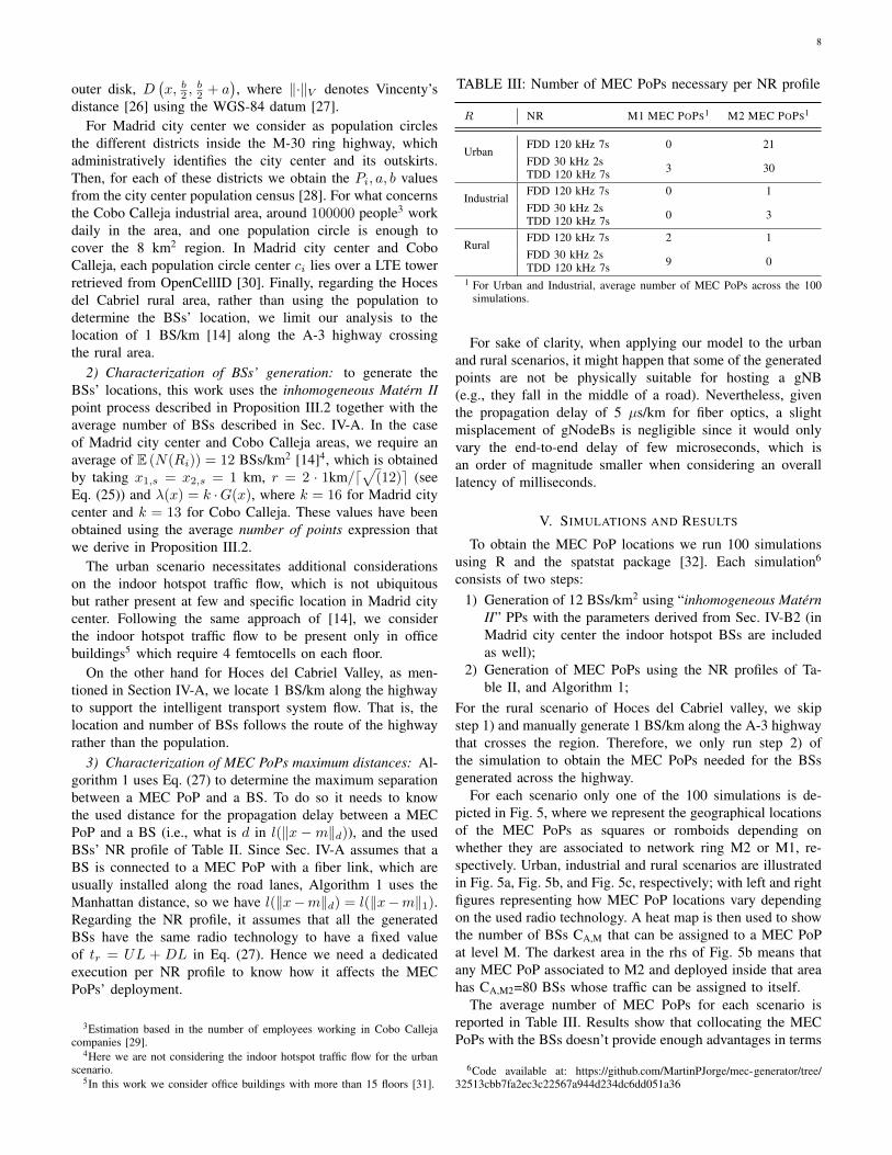
TABLE III: Number of MEC PoPs necessary per NR profile

R NR M1 MEC POPS1 M2 MEC POPS1

UrbanFDD 120 kHz 7s 0 21FDD 30 kHz 2sTDD 120 kHz 7s 3 30

IndustrialFDD 120 kHz 7s 0 1FDD 30 kHz 2sTDD 120 kHz 7s 0 3

RuralFDD 120 kHz 7s 2 1FDD 30 kHz 2sTDD 120 kHz 7s 9 0

1 For Urban and Industrial, average number of MEC PoPs across the 100simulations.

For sake of clarity, when applying our model to the urbanand rural scenarios, it might happen that some of the generatedpoints are not be physically suitable for hosting a gNB(e.g., they fall in the middle of a road). Nevertheless, giventhe propagation delay of 5 µs/km for fiber optics, a slightmisplacement of gNodeBs is negligible since it would onlyvary the end-to-end delay of few microseconds, which isan order of magnitude smaller when considering an overalllatency of milliseconds.

V. SIMULATIONS AND RESULTS

To obtain the MEC PoP locations we run 100 simulationsusing R and the spatstat package [32]. Each simulation6

consists of two steps:1) Generation of 12 BSs/km2 using “inhomogeneous Matern

II” PPs with the parameters derived from Sec. IV-B2 (inMadrid city center the indoor hotspot BSs are includedas well);

2) Generation of MEC PoPs using the NR profiles of Ta-ble II, and Algorithm 1;

For the rural scenario of Hoces del Cabriel valley, we skipstep 1) and manually generate 1 BS/km along the A-3 highwaythat crosses the region. Therefore, we only run step 2) ofthe simulation to obtain the MEC PoPs needed for the BSsgenerated across the highway.

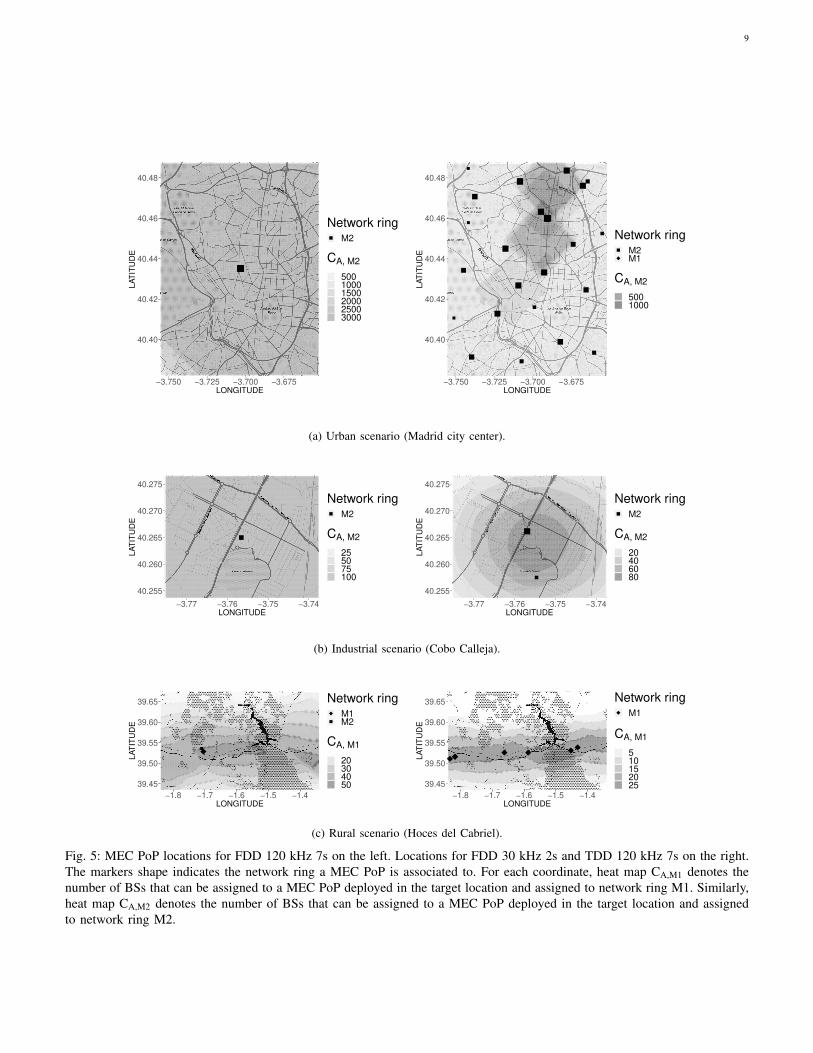
For each scenario only one of the 100 simulations is de-picted in Fig. 5, where we represent the geographical locationsof the MEC PoPs as squares or romboids depending onwhether they are associated to network ring M2 or M1, re-spectively. Urban, industrial and rural scenarios are illustratedin Fig. 5a, Fig. 5b, and Fig. 5c, respectively; with left and rightfigures representing how MEC PoP locations vary dependingon the used radio technology. A heat map is then used to showthe number of BSs CA,M that can be assigned to a MEC PoPat level M. The darkest area in the rhs of Fig. 5b means thatany MEC PoP associated to M2 and deployed inside that areahas CA,M2=80 BSs whose traffic can be assigned to itself.

The average number of MEC PoPs for each scenario isreported in Table III. Results show that collocating the MECPoPs with the BSs doesn’t provide enough advantages in terms

6Code available at: https://github.com/MartinPJorge/mec-generator/tree/32513cbb7fa2ec3c22567a944d234dc6dd051a36

9

40.40

40.42

40.44

40.46

40.48

−3.750 −3.725 −3.700 −3.675LONGITUDE

LAT

ITU

DE

Network ringM2

CA, M2

50010001500200025003000

40.40

40.42

40.44

40.46

40.48

−3.750 −3.725 −3.700 −3.675LONGITUDE

LAT

ITU

DE

Network ringM2M1

CA, M2

5001000

(a) Urban scenario (Madrid city center).

40.255

40.260

40.265

40.270

40.275

−3.77 −3.76 −3.75 −3.74LONGITUDE

LAT

ITU

DE

Network ringM2

CA, M2

255075100

40.255

40.260

40.265

40.270

40.275

−3.77 −3.76 −3.75 −3.74LONGITUDE

LAT

ITU

DE

Network ringM2

CA, M2

20406080

(b) Industrial scenario (Cobo Calleja).

39.45

39.50

39.55

39.60

39.65

−1.8 −1.7 −1.6 −1.5 −1.4LONGITUDE

LAT

ITU

DE

Network ringM1M2

CA, M1

20304050 39.45

39.50

39.55

39.60

39.65

−1.8 −1.7 −1.6 −1.5 −1.4LONGITUDE

LAT

ITU

DE

CA, M1

510152025

Network ringM1

(c) Rural scenario (Hoces del Cabriel).

Fig. 5: MEC PoP locations for FDD 120 kHz 7s on the left. Locations for FDD 30 kHz 2s and TDD 120 kHz 7s on the right.The markers shape indicates the network ring a MEC PoP is associated to. For each coordinate, heat map CA,M1 denotes thenumber of BSs that can be assigned to a MEC PoP deployed in the target location and assigned to network ring M1. Similarly,heat map CA,M2 denotes the number of BSs that can be assigned to a MEC PoP deployed in the target location and assignedto network ring M2.

10

0

0.33

0.66

1

6 20 40 60 80 100 120 144

eC

DF

#radio heads associated to a MEC PoP

Industrial (Cobo Calleja)

Urban (Madrid city center)

Rural (Hoces del Cabriel)

FDD 120 kHz 7s

TDD 120 kHz 7s

FDD 30 kHz 2s

Fig. 6: eCDF of the number of BSs assigned to a MEC PoPin the studied scenarios.

of BSs aggregation and target traffic delay requirement. This isbecause the network delay (see Eq. (28)) can be satisfactorilyfulfilled by aggregating more BSs in fewer MEC PoPs athigher network rings (e.g., M1, M2, etc.). In fact, Algorithm 1minimizes the number of MEC PoPs whilst fulfilling thetraffic requirements. Such traffic requirements (e.g., 1 ms RTTconstraint for the URLLC slice) are never satisfied when theMEC PoPs are located at the M3 and M4 network rings,yielding to empty matrices[M3] and matrices[M4]. Thereason of such behavior is that packet processing delay (seeEq. (28)) increases linearly with the number of network ringsto be traversed. As a result, the MEC PoPs have been alwaysassociated to M1 or M2 network rings in all our simulations,as it can be appreciated in one of the simulation realizationsshown in Fig. 5.

The lower the packet processing time, the higher the max-imum distance between a BS and a MEC PoP (see Eq. (28)).Thus MEC PoPs associated to M1 have more candidate BSsto be assigned than MEC PoPs associated to M2. But amongall the candidate BSs it can only have 6 BSs assigned, while aMEC PoP associated to M2 can have up to 144 BSs assigned.For both the urban and industrial scenarios, the results of our100 simulations (see Table III) show that most of the MECPoPs are associated to M2. Since both scenarios have shortdistances and propagation delays because of the high densityof BSs/km2, the addition of M2 packet processing delay doesnot exceed the 1 ms RTT of URLLC. Therefore, Algorithm 1associates the MEC PoPs to the M2 network ring, and assignsthem as many BSs as possible to reduce the number of MECPoPs. Conversely, looking to Figure 5c, more MEC PoPs areassociated to M1 in the rural scenario because distances andpropagation delay to BSs are high enough to exceed the 1 msRTT when MEC PoPs are associated to M2.

Regarding the different NR profiles (see Table II), low ULand DL delays of FDD 120 kHz 7s permit to increase themaximum distance between a BS and a MEC PoP. Therefore,a MEC PoP can serve a larger number of BSs, as shown inthe darker heat maps at the lhs of Fig. 5. As a result, usingFDD 120 kHz 7s as NR profile necessitates the deployment offewer MEC PoPs compared to all the other NR profiles (seeTable III). Indeed, any MEC PoP location in the urban andindustrial scenario can serve any FDD 120 kHz 7s BSs in theregion as shown in Fig. 5a and Fig. 5b. Instead, FDD 30 kHz2s and TDD 120 kHz 7s impose a higher UL and DL delay,

thus requiring a shorter distance between a BS and a MECPoP. This results in a larger number of MEC PoPs sparselylocated in the region (see rhs of Fig. 5).

Fig. 6 illustrates the experimental Cumulative Density Func-tion (eCDF) for the number of BSs assigned to a MECPoP. Results show that the FDD 120 kHz 7s NR technologyincreases the number of BSs associated to a MEC PoP (lessthan the 33% of them have less than 100 BSs assigned in theindustrial and urban scenario), while the other NR technologieslead to a higher percentage of MEC PoPs with fewer BSsassigned. For example, 68% of the MEC PoPs of the industrialscenario have less than 70 BSs assigned when TDD 120 kHz7s or FDD 30 kHz 2s are used, which is less than half theBSs that can be assigned to a MEC PoP associated to M2.

Summarizing, there is a trade-off between the performanceof the NR profile and the number of MEC PoPs. Higher per-formance radio profiles, which can be more expensive, allowto associate a larger number of BSs to a MEC PoP, resultingin fewer MEC PoPs. On the contrary, a less performant radioprofile, which is cheaper, requires a large number of MECPoPs for satisfying URLLC traffic. This trade-off should betaken into consideration by the network operators to optimizecosts when building their network.

VI. CONCLUSIONS AND FUTURE WORK

In this article we have presented a mathematical model todetermine the deployment of Base Stations (BSs) and MECPoints of Presence (PoPs), using novel point processes thataccount for both people population and minimum distancesbetween BSs. The model is applied in real urban, industrialand rural scenarios, where we generate 5G gNodes B and MECdeployments that satisfy the strictest 5G latency constraint ofUltra-Reliable and Low Latency Communications (URLLC)slices, and thus can support future Augmented Reality/VirtualReality (AR/VR) and low latency streaming services. We havealso analyzed the use of 3 future New Radio (NR) profilesof 5G and simulations show that FDD 120 kHz 7s is thetechnology that minimizes the number of MEC PoPs neededto support the future traffic demands. Future directions ofthis work include the analysis of the resource requirementsof the MEC PoPs, the usage of clustering techniques for theassignment of BSs to MEC PoPs, and the formulation ofan optimization problem to minimize MEC PoP deploymentcosts.

REFERENCES

[1] 3GPP, “System Architecture for the 5G System,” 3rd Generation Part-nership Project (3GPP), Technical Specification (TS) 23.501 v15.4.0, 122018.

[2] L. Han, S. Appleby, and K. Smith, “Problem statement:Transport support for augmented and virtual reality applications,”Working Draft, IETF Secretariat, Internet-Draft draft-han-iccrg-arvr-transport-problem-00, March 2017, http://www.ietf.org/internet-drafts/draft-han-iccrg-arvr-transport-problem-00.txt.[Online]. Available: http://www.ietf.org/internet-drafts/draft-han-iccrg-arvr-transport-problem-00.txt

[3] Z. Shi, H. Zou, M. Rank, L. Chen, S. Hirche, and H. J. Muller, “Effectsof packet loss and latency on the temporal discrimination of visual-haptic events,” IEEE Transactions on Haptics, vol. 3, no. 1, pp. 28–36,Jan 2010.

11

[4] Y. C. Hu, M. Patel, D. Sabella, N. Sprecher, and V. Young, “Mobileedge computing – A key technology towards 5G,” ETSI White Paper,vol. 11, 2015.

[5] F. Giust, X. Costa-Perez, and A. Reznik, “Multi-Access Edge Comput-ing: An Overview of ETSI MEC ISG,” IEEE 5G Tech Focus, vol. 1,no. 4, 2017.

[6] V. Suryaprakash, P. Rost, and G. Fettweis, “Are Heterogeneous Cloud-Based Radio Access Networks Cost Effective?” IEEE Journal onSelected Areas in Communications, vol. 33, no. 10, pp. 2239–2251, Oct2015.

[7] A. Baddeley, C. internazionale matematico estivo, and W. Weil, Stochas-tic Geometry: Lectures Given at the C.I.M.E. Summer School Held inMartina Franca, Italy, September 13-18, 2004, ser. Lecture Notes inMathematics / C.I.M.E. Foundation Subseries. Springer, 2007.

[8] V. Suryaprakash, J. Mller, and G. Fettweis, “On the Modeling and Anal-ysis of Heterogeneous Radio Access Networks Using a Poisson ClusterProcess,” IEEE Transactions on Wireless Communications, vol. 14, no. 2,pp. 1035–1047, Feb 2015.

[9] J. Neyman and E. L. Scott, “Statistical Approach to Problemsof Cosmology,” Journal of the Royal Statistical Society. Series B(Methodological), vol. 20, no. 1, pp. 1–43, 1958. [Online]. Available:http://www.jstor.org/stable/2983905

[10] A. M. Ibrahim, T. ElBatt, and A. El-Keyi, “Coverage probability analysisfor wireless networks using repulsive point processes,” in 2013 IEEE24th Annual International Symposium on Personal, Indoor, and MobileRadio Communications (PIMRC), Sept 2013, pp. 1002–1007.

[11] M. Afshang and H. S. Dhillon, “Poisson cluster process based analysisof hetnets with correlated user and base station locations,” IEEE Trans-actions on Wireless Communications, vol. 17, no. 4, pp. 2417–2431,April 2018.

[12] M. Syamkumar, P. Barford, and R. Durairajan, “DeploymentCharacteristics of ”The Edge” in Mobile Edge Computing,” inProceedings of the 2018 Workshop on Mobile Edge Communications,ser. MECOMM’18. New York, NY, USA: ACM, 2018, pp. 43–49.[Online]. Available: http://doi.acm.org/10.1145/3229556.3229557

[13] V. Frascolla, F. Miatton, G. K. Tran, K. Takinami, A. D. Domenico,E. C. Strinati, K. Koslowski, T. Haustein, K. Sakaguchi, S. Barbarossa,and S. Barberis, “5G-MiEdge: Design, standardization and deploymentof 5G phase II technologies: MEC and mmWaves joint development forTokyo 2020 Olympic games,” in 2017 IEEE Conference on Standardsfor Communications and Networking (CSCN), Sept 2017, pp. 54–59.

[14] L. Cominardi, L. M. Contreras, C. J. Bcrnardos, and I. Berberana,“Understanding QoS Applicability in 5G Transport Networks,” in 2018IEEE International Symposium on Broadband Multimedia Systems andBroadcasting (BMSB), June 2018, pp. 1–5.

[15] B. Matern, Spatial Variation, ser. (Meddelanden fran Statens Skogs-forskningsinstitut). Springer New York, 1986.

[16] R. Schneider and W. Weil, Stochastic and Integral Geometry, ser.Probability and its Applications. Berlin, Germany: Springer, 2008.

[17] NGMN, “Description of Network Slicing Concept,” Next GenerationMobile Networks Alliance, White Paper v1.0, 2 2016.

[18] 3GPP, “Service requirements for next generation new services andmarkets,” 3rd Generation Partnership Project (3GPP), Technical Speci-fication (TS) 22.261, 09 2018, version 16.5.0.

[19] NGMN, “5G White Paper,” Next Generation Mobile Networks Alliance,White Paper v1.0, 2 2015.

[20] ITU-T, “Consideration on 5G transport network reference architectureand bandwidth requirements,” International Telecommunication Union- Telecommunication Standardization Sector (ITU-T), Study Group 15Contribution 0462, 2 2018.

[21] F. Cavaliere et al., “Towards a unified fronthaul-backhaul data planefor 5G The 5G-Crosshaul project approach,” Computer Standards &Interfaces, vol. 51, pp. 56–62, 2017.

[22] EANTC, “Juniper Networks MPC9E: EANTC Performance, Scale andPower Test Report,” European Advanced Networking Test Center, WhitePaper v1.0, 4 2016.

[23] ——, “Huawei 5G-Ready SDN: Evaluation of the Transport NetworkSolution,” European Advanced Networking Test Center, Tech. Rep., 092018.

[24] J. Sachs, G. Wikstrom, T. Dudda, R. Baldemair, and K. Kittichokechai,“5G Radio Network Design for Ultra-Reliable Low-Latency Communi-cation,” IEEE Network, vol. 32, no. 2, pp. 24–31, March 2018.

[25] R. Burden and J. Faires, Numerical Analysis. Brooks/Cole, CengageLearning, 2011. [Online]. Available: https://books.google.it/books?id=KlfrjCDayHwC

[26] T. Vincenty, “Direct and inverse solutions of geodesics on the ellipsoidwith application of nested equations,” Survey Review, vol. 23, no. 176,pp. 88–93, 1975.

[27] W3C, “WGS84 Geo Positioning,” 2006.[28] Padron Municipal de Habitantes, “Poblacion por distrito y barrio,”

http://www-2.munimadrid.es/TSE6/control/seleccionDatosBarrio, 2018,[Accessed: 2018-10-17].

[29] Registro Mercantil y de Bienes Muebles de laProvincia de Madrid, “Registro Mercantil de Madrid,”https://www.rmercantilmadrid.com/RMM/Home/Index.aspx, 2018,[Accessed: 2018-08-27].

[30] “OpenCellID,” http://opencellid.org, 2018, [Accessed: 2018-08-31].[31] Ministerio de Hacienda, “Sede Electronica del Catastro,”

http://www.sedecatastro.gob.es/, 2018, [Accessed: 2018-09-21].[32] A. Baddeley, E. Rubak, and R. Turner, Spatial Point Patterns:

Methodology and Applications with R. London: Chapman andHall/CRC Press, 2015. [Online]. Available: http://www.crcpress.com/Spatial-Point-Patterns-Methodology-and-Applications-with-R/Baddeley-Rubak-Turner/9781482210200/