modeling human interactions as a network of kuramoto’s

Escola Tecnica Superior d’Enginyeria Industrial deBarcelona

Universitat Politecnica de Catalunya

Modeling human interactions as anetwork of Kuramoto’s oscillators

Master’s Thesis

Master’s Degree in Industrial Engineering

AUTHOR: Albert David Gil MartınezSUPERVISOR: Prof. Mario di Bernardo

2019

Contents

1 Introduction 11.1 State of the art . . . . . . . . . . . . . . . . . . . . . . . . . . . . . . . . . . 2

2 Synchronization in a network of oscillators 42.1 Kuramoto’s Model . . . . . . . . . . . . . . . . . . . . . . . . . . . . . . . . 42.2 Kinds of synchronization . . . . . . . . . . . . . . . . . . . . . . . . . . . . . 62.3 Measuring synchronization . . . . . . . . . . . . . . . . . . . . . . . . . . . . 8

2.3.1 Order Parameter . . . . . . . . . . . . . . . . . . . . . . . . . . . . . 82.3.2 Other parameters to measure synchronization . . . . . . . . . . . . . 8

3 Modeling human coordination 123.1 Setup and experimental data . . . . . . . . . . . . . . . . . . . . . . . . . . . 123.2 Modeling human interaction as a network of Kuramoto’s oscillators . . . . . 153.3 Limitations of the model . . . . . . . . . . . . . . . . . . . . . . . . . . . . . 16

4 Improvement of the model 174.1 First Attempt . . . . . . . . . . . . . . . . . . . . . . . . . . . . . . . . . . . 174.2 Second Attempt . . . . . . . . . . . . . . . . . . . . . . . . . . . . . . . . . . 194.3 Third Attempt . . . . . . . . . . . . . . . . . . . . . . . . . . . . . . . . . . 214.4 Fourth Attempt . . . . . . . . . . . . . . . . . . . . . . . . . . . . . . . . . . 244.5 Fifth Attempt . . . . . . . . . . . . . . . . . . . . . . . . . . . . . . . . . . . 264.6 Sixth Attempt . . . . . . . . . . . . . . . . . . . . . . . . . . . . . . . . . . . 284.7 Considerations . . . . . . . . . . . . . . . . . . . . . . . . . . . . . . . . . . 30

4.7.1 Simulations Group 2 . . . . . . . . . . . . . . . . . . . . . . . . . . . 304.7.2 Simulations Group 3 . . . . . . . . . . . . . . . . . . . . . . . . . . . 314.7.3 Summary . . . . . . . . . . . . . . . . . . . . . . . . . . . . . . . . . 33

5 Conclusions 34

List of Figures

2.1 Two different groups of oscillators (first row and second row), for differentvalues of the coupling parameter. In the first row oscillators share the samenatural frequency. . . . . . . . . . . . . . . . . . . . . . . . . . . . . . . . . . 5

2.2 Frequency ωk of oscillators in two different conditions. In (a) with a value ofc below the threshold, in (b) over it. . . . . . . . . . . . . . . . . . . . . . . . 6

2.3 Phase-locking. In (a) is represented the phase of each oscillator. In (b) isrepresented the frequency of each oscillator. . . . . . . . . . . . . . . . . . . 7

2.4 Phase-synchronization. In (a) is represented the phase of each oscillator. In(b) is represented the frequency of each oscillator. . . . . . . . . . . . . . . . 7

2.5 Value of r for two different situations. In (a) and (b) there is no synchroniza-tion, in (c) and (d) there is phase-locking. . . . . . . . . . . . . . . . . . . . 9

2.6 Order parameter and group synchronization index computed for two differentsituations, with phase-locking and with phase-synchronization. . . . . . . . . 11

3.1 Different network topologies. . . . . . . . . . . . . . . . . . . . . . . . . . . . 133.2 Topology all-to all of the network of simulation 1, Group 1. . . . . . . . . . . 153.3 Frequency of each player in simulation 1, Group 1. . . . . . . . . . . . . . . . 16

4.1 Frequency of each player in simulation 2, Group 1. . . . . . . . . . . . . . . . 184.2 Frequency of each player in simulation 3, Group 1. . . . . . . . . . . . . . . . 194.3 Simulations with a ring graph, Group 1. . . . . . . . . . . . . . . . . . . . . 204.4 Frequency of each player in simulation 4, Group 1. . . . . . . . . . . . . . . . 214.5 Relation between a leader personality and standard deviation in the solo con-

dition. . . . . . . . . . . . . . . . . . . . . . . . . . . . . . . . . . . . . . . . 224.6 Frequency of each player in simulation 5, Group 1. . . . . . . . . . . . . . . . 234.7 Synchronization in Third Attempt, Group 1. . . . . . . . . . . . . . . . . . . 234.8 Frequency of each player in simulation 6, Group 1. . . . . . . . . . . . . . . . 244.9 Synchronization in Fourth Attempt, Group 1. . . . . . . . . . . . . . . . . . 254.10 Frequency of each player in simulation 7, Group 1. . . . . . . . . . . . . . . . 254.11 Synchronization in Fifth Attempt, Group 1. . . . . . . . . . . . . . . . . . . 264.12 Topology all-to all of the network of simulation 8, Group 1. . . . . . . . . . . 274.13 Frequency of each player in simulation 8, Group 1. . . . . . . . . . . . . . . . 284.14 Synchronization in Sixth Attempt, Group 1. . . . . . . . . . . . . . . . . . . 294.15 Frequency of each player in simulation 9, Group 1. . . . . . . . . . . . . . . . 294.16 Topology all-to all of the network of simulation 11, Group 2. . . . . . . . . . 30

LIST OF FIGURES

4.17 Simulations with dataset of Group 2. In (a) the frequency of each player withthe Third Attempt is represented, Simulation 10. In (b) the frequency of eachplayer with the Fifth Attempt is represented, Simulation 11. . . . . . . . . . 31

4.18 Topology all-to all of the network of simulation 13, Group 3. . . . . . . . . . 324.19 Simulations with dataset of Group 3. In (a) and (c) is represented the fre-

quency of each player with the Third Attempt, Simulation 12. In (b) and(d) and is represented the frequency of each player with the Fifth Attempt,Simulation 13. . . . . . . . . . . . . . . . . . . . . . . . . . . . . . . . . . . . 33

iii

Chapter 1

Introduction

Understanding how humans coordinate when they have to perform a joint task is an importantproblem in Human Behaviour Science. Motor coordination is required in a lot of humanactivities, for instance hands clapping in an audience, walking in a crowd, music playing,sports or dance. Let us consider, for example a cycling team. In order to follow the rateof the instructor, people have to synchronise their pedals to achieve the reference speed. Innature, an example is represented by the synchronous flashing of fireflies observed in someSouth Asia forests. At night, a myriad of fireflies lay over the trees. Suddenly, several firefliesstart emitting flashes of light. Initially, they flash incoherently, but after a short period oftime the whole swarm is flashing in unison creating one of the most striking visual effectsever seen. Synchronisation has not always been fully understood in nature, in the case offireflies, synchronization may facilitate the courtship between males and females, but in othercases the biological role of synchronisation is under discussion. This and other examples ofsynchronisation in nature can be found in [1].

Moreover, research in Human Science suggests that social motor coordination is linked to thefeeling of mental connectedness between individuals [2]. Consequently understanding howthis coordination emerges in a group of individuals can help to develop innovative rehabilita-tion strategies for patients suffering from social disorders [3]. Creating a customized virtualplayer (a robot or a computer-generated avatar) able to interact with the patient would be ofgreat help. In addition, the more we know about how humans behave in a group, the bettera robot can be programmed to behave like a real human.

In our daily life coordinated movements of two or more people mirroring each other, frequentlyoccur. The mirror game provides a simple paradigmatic example to investigate the onset ofsocial motor coordination between two or more human players. In its simplest formulation,two players are asked to create synchronized sinusoidal movements of their forearms, withouta designated leader. Given the oscillatory nature of the task, the player’s dynamics can bemodelled through a network of interacting oscillators [4]. In this research, we adapt the mirrorgame to study synchronization in multiplayer human ensembles. We asked three groups ofseven volunteers to carry out a joint task in which they had to generate and synchronize an

CHAPTER 1. INTRODUCTION

oscillatory motion of their preferred hand. The task is done in two different conditions: solocondition and group condition. In solo condition we can capture the intrinsic frequency oftheir hand movements and in the group condition we can capture the frequency when theyreach synchronization. We found out that the synchronization frequency in group conditionis notably smaller than the mean frequency of all the players in solo condition, there issome unknown social interaction between players that makes decrease their velocities. Firstattempts to model this behaviour with MATLAB [5] applying Kuramoto’s model [6] havenot been successful, because it is not able to capture the decreasing in frequency observedexperimentally when players reach synchronization. Therefore, the aim of this work is theanalysis and the improvement of a model based on a network of Kuramoto’s oscillators ableto reproduce experimental results.

1.1 State of the art

The problem of how coordination emerges in human ensembles has been rarely studied quan-titatively in the existing literature. It is because performing synchronisation in a humangroup involves perceptual interaction through sound, feel, or sight and the establishment ofmental connectedness and social attachment among group members, all of this makes itsstudy challenging [7]. However, there are researches on situations involving dual interaction[8][9] or on situations including dynamics of animal groups [10][11].

In human ensembles, results are mostly experimental observations of group behaviour, forinstance studies on rocking chairs [12], rhythmic activities and marching tasks [13], choirsingers during a concert, group synchronisation of arm movements and respiratory rhythms[14], teams rowing a race [15] and others sport situations [16]. These studies have analysedthe emergent level of coordination in the group. In [17] an interactive control architectureis developed to generate human-like trajectories in the mirror game, a simple yet effectiveparadigm for studying interpersonal coordination. Also, an online control algorithm for thearchitecture is proposed to produce joint improvised motion with a human player or anothervirtual player while exhibiting some desired kinematic characteristics. Other studies in [18]have shown that the outcome and the quality of the performance in a number of situationsstrongly depend on how the individuals in the ensemble exchange visual, auditory and motorinformation. For instance, in [19] researchers studied synchronization in multiplayer humanensembles. It is observed that despite the complexity of social interactions a network ofheterogeneous Kuramoto oscillators behaves like a human ensemble. They found that thecoordination level of the participants in two different ensembles varied over different topolo-gies and that such variations were more significant in the group characterised by a higherheterogeneity in terms of the natural oscillation frequency of its members. But there areother fields where the synchronization phenomena between large populations of interactingelements take place, for example in physics, biology and chemistry. A successful approach tothe problem consists of modelling each member of the population as a phase oscillator, dueto the oscillatory nature of the phenomena of interest [20].

2

CHAPTER 1. INTRODUCTION

In this project, synchronisation is going to be analysed in one of the most representative mod-els of coupled phase oscillators, the Kuramoto’s model [6]. Rigorous mathematical treatment,specific numerical methods, and many variations and extensions of the original model thathave appeared in the last years are presented in [20]. This work will extend the knowl-edge of how people synchronise when they have to perform a joint task, using a network ofheterogeneous Kuramoto oscillators.

3

Chapter 2

Synchronization in a network ofoscillators

In this chapter the generalized Kuramoto’s model of coupled oscillators is described, as wellas different kinds of synchronization. Additionally, ways to measure synchronization arepresented in the following sections.

2.1 Kuramoto’s Model

The Kuramoto’s model consists of a population of N coupled phase oscillators θk(t), havingnatural frequencies ωk, and whose dynamics are governed by Eq. 2.1, where akh representsthe element of the adjacency matrix, that is a square matrix used to represent a finite graph.The elements of the matrix akh indicate whether pairs of vertices (k, h) are adjacent or not inthe graph, in other words, if the oscillators are connected between them or not. Consequently,each oscillator tries to run independently at its own frequency, while the coupling c weights thecontribution of adaptation of their angular velocites based on the phase mismatch. Whenthe coupling is weak, the oscillators run incoherently, whereas beyond a certain thresholdcollective synchronization emerges spontaneously [21]. In [22] is shown that if the coupling issufficiently large and the natural frequencies of each oscillator are equal, then for a networkwith all-to-all links, synchronization to the aligned state (same phase and frequency) isglobally achieved for all initial states. Moreover, the consensus value ωsync when oscillatorsreach synchronization in frequency is governed by Eq. 2.2, that is indeed the average of theoscillators natural frequencies.

θk = wk + cN∑h=1

akhsin(θh − θk), k = 1, 2, ..., N (2.1)

CHAPTER 2. SYNCHRONIZATION IN A NETWORK OF OSCILLATORS

ωsync =1

N

N∑k=1

ωk (2.2)

In Fig. 2.1 we can see two systems of 10 oscillators each one represented by dots, createdusing [23]. The state of each oscillator is represented by θk whereas ωk represents its naturalfrequency that captures how fast the oscillator would move on the unitary circle if it wasuncouples. In the figure dots are shaded according to their natural frequency, brighter dotsmove faster than dark ones. The vector that appears in the middle of the image with a reddot at the tip represents the order parameter of the system (see section 2.3.1), that quantifythe degree and onset of synchronization. If all dots are scattered uniformly around the circlethe order parameter is close to zero, if they are all moving in phase synchronization it isequal to one. In Fig. 2.1a and Fig. 2.1d oscillators are uncoupled (c = 0) and randomlydistributed on the circle. In Fig. 2.1a to Fig. 2.1c the oscillators have the same naturalfrequencies therefore the network is homogeneous. Looking at Fig. 2.1b, Fig. 2.1c, Fig. 2.1e,and Fig. 2.1f we can see how oscillators are now more grouped, this is because frequencysynchronization is emerging. In Fig. 2.1c oscillators reach also phase synchronization thanksto their homogeneity.

(a) c = 0. (b) c > 0. (c) c� 0.

(d) c = 0. (e) c > 0. (f) c� 0.

Figure 2.1: Two different groups of oscillators (first row and second row), for different valuesof the coupling parameter. In the first row oscillators share the same natural frequency.

In Fig. 2.2 we can see the frequencies of 5 oscillators in a simulation of 10 seconds, with avalue of the coupling parameter c below and over the threshold, beginning from the same

5


initial conditions shown in Table 2.1. In Fig. 2.2a it can be seen how oscillators do not reachfrequency synchronization because c is below the threshold, whereas in Fig. 2.2b oscillatorssynchronize in frequency, reaching a value ωsync = 5 rad/s. We can check this value satisfyEq. 2.2. As a result, we can conclude in this specific case the threshold is between c = [1, 2].

Oscillator 1 Oscillator 2 Oscillator 3 Oscillator 4 Oscillator 5ωk[rad/s] 0.57 3.36 7.23 3.28 10.54θk0[rad] -2.25 -0.49 2.61 1.84 2.89

Table 2.1: Initial conditions in Kuramoto’s Model.

(a) c = 1. (b) c = 2.

Figure 2.2: Frequency ωk of oscillators in two different conditions. In (a) with a value of cbelow the threshold, in (b) over it.

2.2 Kinds of synchronization

Synchronization is considered when there is an interaction between oscillators that naturallyyields perfect or partial synchrony, in their frequencies ωk or in their phases θk. Therefore,it may be two different types:

• Phase-locking. There is phase-locking when oscillators synchronize their frequencies,limt→∞(θk − θh) = 0, consequently they keep their phases locked one from each other.In Fig. 2.3 the phases of 5 oscillators are represented with the initial conditions shownin Table 2.1 and with c = 2 for a simulation of 10 seconds. We can see how theysynchronize their frequencies but not their phases.

6


• Phase-synchronization. There is phase-synchronization when the phases of the os-cillators converge to a common trajectory, limt→∞(θk − θh) = 0. Consequently, theyare also synchronized in frequency, the second type of synchronization implies the firstone but not vice versa. In order to reach phase-synchronization oscillators have toshare the same natural frequencies as seen in section 2.1. In Fig. 2.4 the phases of 5oscillators are represented with the initial conditions shown in Table 2.1 but this timewith natural frequencies ωk = 5 rad/s and with c = 2 for a simulation of 10 seconds.We can see how they synchronize their phases.

(a) Phases. (b) Frequencies.

Figure 2.3: Phase-locking. In (a) is represented the phase of each oscillator. In (b) isrepresented the frequency of each oscillator.

(a) Phases. (b) Frequencies.

Figure 2.4: Phase-synchronization. In (a) is represented the phase of each oscillator. In (b)is represented the frequency of each oscillator.

7


2.3 Measuring synchronization

It has been shown that oscillators with dynamics governed by Eq. 2.1 can synchronizetheir frequencies. In section 2.2 we have seen different types of synchronization so there aredifferent degrees of synchronization. It is needed a way to measure how much the oscillatorsare synchronized.

2.3.1 Order Parameter

The order parameter is described in Eq. 2.3 in his complex form, where r ∈ [0, 1] representsthe phase-coherence of the population of oscillators and ψ indicates the group phase. Whenthere is completely synchronization in phase, r reaches its maximum value.

reiψ =1

N

N∑k=1

eiθk (2.3)

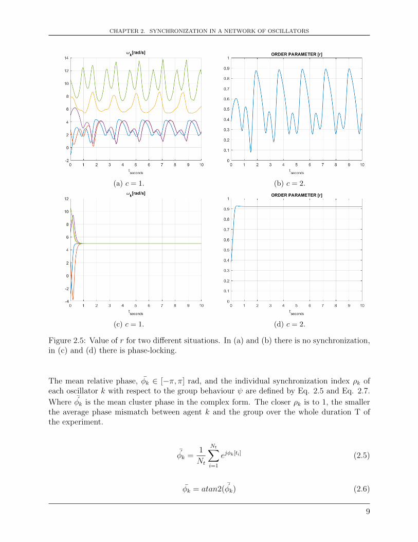
In Fig. 2.5a we can see a simulation with initial conditions shown in Table 2.1 and with avalue of the coupling parameter below the threshold of frequency synchronization. On theother hand, in Fig. 2.5c we can see a simulation with the same initial conditions but with avalue of the coupling parameter over the threshold. If we look at r we can see how in Fig.2.5b is oscillating throughout the whole simulation, whereas in Fig. 2.5d its value is close to1.

2.3.2 Other parameters to measure synchronization

We have seen in section 2.3.1 that the order parameter can be used to measure phase synchro-nization in a group of oscillators. There are other parameters like in the Kuramoto basedcluster phase method proposed in [12] that can be used to quantify phase and frequencysynchronization among oscillators, which are going to be presented below. N oscillators andthe time-series θk(t) are considered, where k = 1, ..., N . θk ∈ [−π, π] rad represents the phaseof each oscillator. T is the duration of an acquired signal and Nt is the number of time steps

of duration 4T =T

Nt.

The relative phase of each oscillator, φk ∈ [−π, π] rad, with respect to the average phase ofthe group ψ at time t is defined by Eq. 2.4.

φk(t) = θk(t)− ψ(t) (2.4)

8


(a) c = 1. (b) c = 2.

(c) c = 1. (d) c = 2.

Figure 2.5: Value of r for two different situations. In (a) and (b) there is no synchronization,in (c) and (d) there is phase-locking.

The mean relative phase, φk ∈ [−π, π] rad, and the individual synchronization index ρk ofeach oscillator k with respect to the group behaviour ψ are defined by Eq. 2.5 and Eq. 2.7.

Where¯φk is the mean cluster phase in the complex form. The closer ρk is to 1, the smaller

the average phase mismatch between agent k and the group over the whole duration T ofthe experiment.

¯φk =

1

Nt

Nt∑i=1

ejφk[ti] (2.5)

φk = atan2(¯φk) (2.6)

9


ρk =∣∣∣ ¯φk

∣∣∣ ∈ [0, 1] (2.7)

In order to quantify the degree of frequency synchronization of the group as a whole attime t is defined the group synchronization index ρg(t) in Eq. 2.8. Similarly to the individualsynchronization index ρk, the closer the group synchronization index ρg(t) is to 1, the smallerthe average frequency mismatch among the agents in the group at time t. Its value can beaveraged over the whole time interval [0, T ] in order to have an estimate of the mean frequencysynchronization level of the group during the total duration of the experiment, giving rise toρg (see Eq. 2.9).

ρg(t) =

∣∣∣∣∣ 1

N

N∑k=1

ej(φk(t)−φk)

∣∣∣∣∣ ∈ [0, 1] (2.8)

ρg =1

NT

NT∑i=1

ρg[ti] ∈ [0, 1] (2.9)

It may seem that the order parameter r and the group synchronization index ρg(t) aremeasuring the same thing, but there is an important difference between them. In Fig.2.6 we have two simulations (first column and second column), if we look at the groupsynchronization index we notice that both reach frequency synchronization (ρg(t) = 1) butby looking the order parameter r we see how there is also phase synchronization in the caseof the second column, because r = 1.

10


(a) Phase-locking. (b) Phase-synchronization.

(c) Group synchronization index. (d) Group synchronization index.

(e) Order parameter. (f) Order parameter.

Figure 2.6: Order parameter and group synchronization index computed for two differentsituations, with phase-locking and with phase-synchronization.

11

Chapter 3

Modeling human coordination

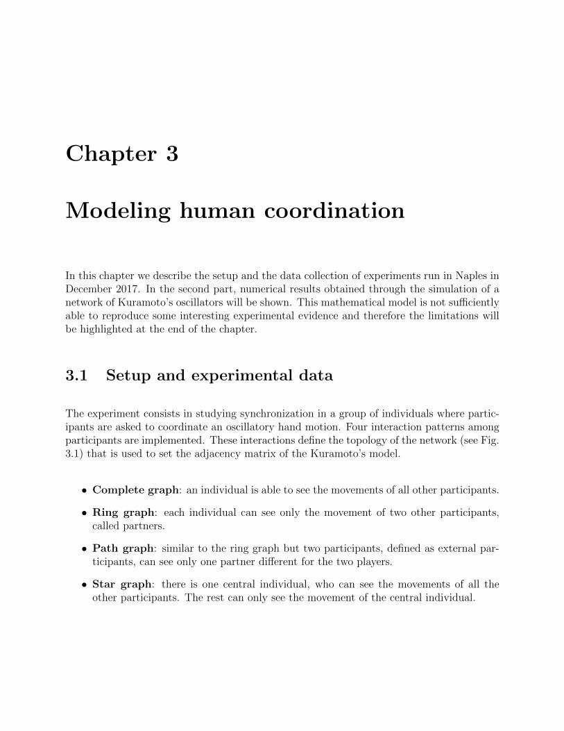
In this chapter we describe the setup and the data collection of experiments run in Naples inDecember 2017. In the second part, numerical results obtained through the simulation of anetwork of Kuramoto’s oscillators will be shown. This mathematical model is not sufficientlyable to reproduce some interesting experimental evidence and therefore the limitations willbe highlighted at the end of the chapter.

3.1 Setup and experimental data

The experiment consists in studying synchronization in a group of individuals where partic-ipants are asked to coordinate an oscillatory hand motion. Four interaction patterns amongparticipants are implemented. These interactions define the topology of the network (see Fig.3.1) that is used to set the adjacency matrix of the Kuramoto’s model.

• Complete graph: an individual is able to see the movements of all other participants.

• Ring graph: each individual can see only the movement of two other participants,called partners.

• Path graph: similar to the ring graph but two participants, defined as external par-ticipants, can see only one partner different for the two players.

• Star graph: there is one central individual, who can see the movements of all theother participants. The rest can only see the movement of the central individual.

CHAPTER 3. MODELING HUMAN COORDINATION

(a) Complete graph. (b) Ring graph.

(c) Path graph. (d) Star graph.

Figure 3.1: Different network topologies.

Participants are asked to sit in front of a computer and move their preferred hand as smoothlyas possible, from left to right. The position of the individual’s hand is represented by a greensolid ball on the computer screen, while the other participants are represented by balls ofdifferent colours. Each group performs the experiments in two different conditions.

• Solo condition: participants are asked to oscillate their preferred hand at their owncomfortable tempo for 30 seconds without seeing the other participants on the screen.In this condition, it can be extracted the natural frequency of each individual.

• Group condition: participants are asked to synchronize the motion of each other’spreferred hands during 30 seconds. This time, they see the ball representing the par-ticipants on the screen. The balls each individual is able to see on the screen dependson the topology of the network for that trial.

13


The experiments have been run through the hardware/software platform Chronos [24][25]plus Leap Motion [26] that is used to detect hand position. Participants have to move theirhands horizontally over the Leap Motion controller with a vertical distance around 15 cmto be sure of the detection of the amplitude of the motion and to guarantee a conformtableheigh . The data obtained, xk[ti] ∈ R, is the discrete time series of the kth agent representingthe motion of each participant’s preferred hand with k ∈ [1, N ] and i ∈ [1, Nt]. N is thenumber of individuals and Nt is the number of time steps of duration 4T =

T

Ntwhere T

is the duration of the experiment and 4T is given by the samply frequency. We extractthe phase, θk(t) ∈ [−π, π] rad, of each signal xk[ti] using the Hilbert transform [27]. Thefrequency of each individual can be extracted applying the Fourier Transform [28] to θk(t),which decomposes a function of time into the frequencies that make it up.

The experiment is done with 3 different groups. In each group there are 5 players and 7trials for solo condition and each topology have been run. The trials have a duration of 30seconds and the sampling frequency is 100 Hz. From the data obtained in the experimentwe compute the mean frequency of each player in the solo and group conditions (see Table3.1 and Table 3.2). It is interesting to notice that the mean frequency in group condition issmaller than the mean frequency in solo condition, whereas this does not happen in Group3 interaction. A possible reason for this different behaviour could be found in the variabilityamong the performance of players in solo condition, 4 players over 5 are not statisticallydifferent among them (except Player 4). This condition could not require players to adaptto each other and, therefore, to modify their natural behaviour.

Player 1 Player 2 Player 3 Player 4 Player 5 MeanGroup1 3.61(±2.25) 3.02(±0.11) 6.82(±0.56) 3.29(±0.16) 10.02(±0.73) 5.35(±0.76)Group2 7.1(±0.66) 7.78(±0.53) 8.31(±0.92) 5.42(±0.21) 3.42(±0.2) 6.41(±0.50)Group3 2.65(±0.25) 2.86(±0.17) 2.79(±0.17) 2.27(±0.24) 2.90(±0.21) 2.69(±0.21)

Table 3.1: Mean frequency (±SD) for all groups [rad/s] in solo condition (ωk,solo).

Complete graph Ring graph Path graph Star graph MeanGroup1 2.95(±0.05) 2.98(±0.32) 2.97(±0.23) 2.81(±0.11) 2.93(±0.18)Group2 4.29(±0.03) 4.46(±0.01) 4.38(±0.02) 4.38(±0.02) 4.38(±0.02)Group3 2.71(±0.12) 2.79(±0.15) 2.85(±0.11) 2.73(±0.2) 2.77(±0.14)

Table 3.2: Mean frequency (±SD) for all groups [rad/s] in group condition (ωk,sync).

14


3.2 Modeling human interaction as a network of Ku-

ramoto’s oscillators

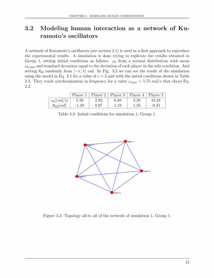
A network of Kuramoto’s oscillators (see section 2.1) is used in a first approach to reproducethe experimental results. A simulation is done trying to replicate the results obtained inGroup 1, setting initial conditions as follows: ωk from a normal distribution with meanωk,solo and standard deviation equal to the deviation of each player in the solo condition. Andsetting θk0 randomly from [−π, π] rad. In Fig. 3.3 we can see the result of the simulationusing the model in Eq. 2.1 for a value of c = 2 and with the initial conditions shown in Table3.3. They reach synchronization in frequency for a value ωsync = 5.75 rad/s that obeys Eq.2.2.

Player 1 Player 2 Player 3 Player 4 Player 5ωk[rad/s] 5.50 2.92 6.88 3.20 10.24θk0[rad] -1.49 0.97 1.19 1.56 -0.31

Table 3.3: Initial conditions for simulation 1, Group 1.

Figure 3.2: Topology all-to all of the network of simulation 1, Group 1.

15


Figure 3.3: Frequency of each player in simulation 1, Group 1.

3.3 Limitations of the model

The results in section 3.2 show us that a network of Kuramoto’s oscillators does not capturethe frequency drop observed experimentally between solo and group condition. For instance,if we focus in Group 1, the mean frequency in group condition is ωsync = 2.93(±0.18) rad/s(see Table 3.2), while the value get in the simulation with the Kuramoto’s model is ωsync =5.75 rad/s. Therefore it is needed an adaptation of the model able to reproduce the behaviourof the participants in the experiment.

16

Chapter 4

Improvement of the model

In this chapter some modifications of the Kuramoto’s model are described to solve its limita-tions. In particular, six attempts are done with different approaches to the problem. We canhighlight two main approaches: in the first we let the player adapt their inner natural fre-quency of oscillation according to the degree of phase synchronization whereas in the secondapproach we let the player weight their connections according to their personality’s traits.

4.1 First Attempt

In this attempt, we want to represent that an individual tends to decrease his velocity un-consciously as he is reaching synchronization with the group. It may be because he is morealert to possible changes in the movements of the other players, so he is focused on keepingsynchronized with the group. The model is described in Eq. 4.1, where we can see that themore the players are in synchronization, the less they adapt to each other.

{θk = wk + c

∑Nh=1 akhsin(θh − θk)

ωk = −(1− r)ωk(4.1)

In all the simulations of this chapter, the initial conditions and the topology of the networkwill be set as follows: ωk will be taken from a normal distribution with mean ωk,solo, the stan-dard deviation from the one observed for each player in the solo condition and θk0 randomlyfrom [−π, π] rad, topologies all-to-all (see Fig. 3.2). Simulating this model for the initialconditions shown in Table 4.1 and a value of c = 2, we get the results shown in Fig. 4.1. Wecan see how participants reach synchronization in frequency but it is decreasing continuouslythroughout the duration of the simulation, therefore it will reach zero for t→∞. Whateverthe value of the cupling parameter is, ωsync will reach zero at infinity because if we look atEq. 4.1 ωk has a minus sign in his definition. However, simulating for the initial conditionsshown in Table 4.2 and a value of c = 12 we see in Fig. 4.2 how at the final of the simulation

CHAPTER 4. IMPROVEMENT OF THE MODEL

players reach frequency synchronization ωsync = 4.90 rad/s. In this case, despite it seems likefrequency is not decreasing, it is really decreasing so slowly that it can not be seen in thegraph.

Player 1 Player 2 Player 3 Player 4 Player 5ωk0[rad/s] 0.57 3.36 7.23 3.28 10.54θk0[rad] -2.25 -0.49 2.61 1.84 2.89


Player 1 Player 2 Player 3 Player 4 Player 5ωk0[rad/s] 1.93 3.14 6.62 3.16 10.06θk0[rad] -0.58 2.64 -0.90 -2.43 -1.54



18


(a) Complete simulation. (b) Detail of the first 3 seconds.


4.2 Second Attempt

The model presented in section 4.1 is not capturing correctly the dynamics observed in theexperiments, but it has also other conceptual problem. An individual is not able to knowthe degree of synchronization with all the other of the group. He is only able to appreciatesynchronization with the players he is able to see, for instance, in some of the topologiesshown in section 3.1 the players are not connected all with all. Due to this, we have defined anew local order parameter described in Eq. 4.2, where only the neighbours of each individual(the other players one is able to see) are computed.

rk =

∣∣∣∣∣ 1

Nneigh,k + 1(N∑h=1

akhejθh + ejθk)

∣∣∣∣∣ (4.2)

In Fig. 4.3 we can see two simulations, the first one using the First Attempt and the secondone using the Second Attempt, this time the topology of the graph is a ring graph (see Fig.3.1) to be able to observe the difference when we include the local order parameter in themodel. The initial conditions are set as shown in Table 4.3 and c = 10.

19


(a) First Attempt, ωsync = 5.28 rad/s. (b) Second Attempt, ωsync = 5.33 rad/s.

Figure 4.3: Simulations with a ring graph, Group 1.

The model with the new local order parameter rk is described in Eq. 4.3. The initialconditions are set as shown in Table 4.3 and the coupling parameter as c=20. From theresults of Fig. 4.4 we can see how players reach synchronization for a value of ωsync = 5.55rad/s, further than in the previous attempt.

{θk = wk + c

∑Nh=1 akhsin(θh − θk)

ωk = −(1− rk)ωk(4.3)

Player 1 Player 2 Player 3 Player 4 Player 5ωk0[rad/s] 5.62 2.93 6.83 3.20 9.23θk0[rad] -0.05 -0.33 -0.08 -2.10 -0.87


20


(a) Complete simulation. (b) Detail of the first 2 seconds.


4.3 Third Attempt

Let us suppose that an individual is connected to two people. In this approach we will weighthis links according to the personality of the player and those of his partners. We want tosymbolize that he tends to follow more the one that has a leading personality. So it is neededa way to define a ’leader personality’. In our experiments a leader personality can be relatedwith the coherence with oneself, that can be represented by the deviation in frequency in thesolo condition (see Fig. 4.5) that is the capability of maintaining a coherent movement indifferent trials . For instance, if the standard deviation of one individual is smaller than theone exhibited by his partner, it means that the first one is more coherent with himself. As aresult, a new model is presented in Eq. 4.4, giving a new definition to akh and where SDk isthe deviation in the solo condition of the player k. So of this way, we have a way to weightthe adjacency matrix and represent how much strong is the connection between players. Inthis model the adjacency matrix is normalized, akh ∈ [0, 1].

21


Figure 4.5: Relation between a leader personality and standard deviation in the solo condi-tion.

θk = wk + cN∑h=1

akhsin(θh − θk), akh =SDk

SDh

∈ [0, 1] (4.4)

We simulate the model Eq. 4.4 with the initial conditions shown in Table 4.4 for a valueof the coupling parameter c=2. The results in Fig. 4.6 show us how the players do notsynchronize in frequency for this value of the coupling parameter, so we want to know forwhich value of the coupling parameter players reach synchronization.

Player 1 Player 2 Player 3 Player 4 Player 5ωk[rad/s] 1.87 2.99 6.90 3.33 9.40θk0[rad] 0.48 2.50 -0.23 -0.64 -2.48


Player 1 Player 2 Player 3 Player 4 Player 5ωk[rad/s] 4.42 2.87 6.21 3.12 10.39θk0[rad] 0.14 -2.42 -2.27 -0.60 -2.14


22



Consequently, 10 simulations are done for each value c ∈ [0, 50]. In Fig.4.7 we can see thenumber of simulations that reach synchronization and the settling time for different values ofthe coupling parameter. Here the settling time is defined as the time players reach a certainvalue of the group synchronization index, in particular ∀t > ts ρg(t) > 0.9. Looking at theplot we can conclude that for a value of c ≥ 13 participants always synchronize in frequency.We simulate with the initial conditions shown in Table 4.5 and for a value of the couplingparameter c=13. In Fig. 4.8 we can see a synchronization frequency of ωsync = 3.15 rad/sthat is very close to the experimental value, ωsync = 2.93± 0.18 (see Table 3.2).

(a) Simulations that reach synchronization. (b) Settling time.

Figure 4.7: Synchronization in Third Attempt, Group 1.

23



4.4 Fourth Attempt

In the Fourth Attempt, we define the elements of the adjacency matrix akh opposite to theThird Attempt. Now individuals are going to follow more other less coherent with themselves(with a higher deviation in frequency in the solo condition). The model is described in Eq.4.5.

θk = wk + c

N∑h=1

akhsin(θh − θk), akh =SDh

SDk

∈ [0, 1] (4.5)

In Fig. 4.9 is represented the number of simulations that reach synchronization of the 10done and the settling time, as seen it in the previous section. We can see that usually thereis at least one simulation for all the values of the coupling parameter where players do notreach synchronization. We can conclude players struggle to reach synchronization comparedwith previous attempts.

24



Figure 4.9: Synchronization in Fourth Attempt, Group 1.

We simulate the model Eq. 4.5 with the initial conditions shown in Table 4.6 and a value of thecoupling parameter c=40. The results in Fig. 4.10 show us the players reach synchronizationfor a value ωsync = 5.97 rad/s.

Player 1 Player 2 Player 3 Player 4 Player 5ωk[rad/s] 5.42 2.94 6.94 3.39 10.79θk0[rad] 2.33 0.61 -1.17 -2.84 -0.56



25


4.5 Fifth Attempt

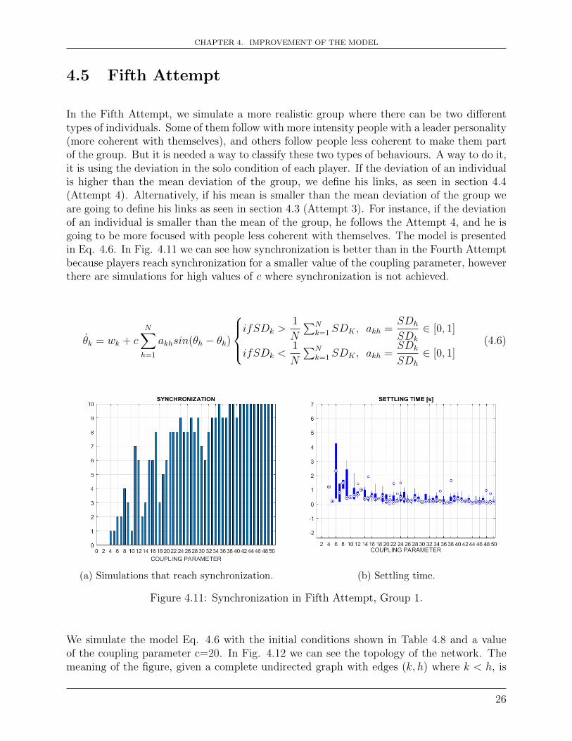
In the Fifth Attempt, we simulate a more realistic group where there can be two differenttypes of individuals. Some of them follow with more intensity people with a leader personality(more coherent with themselves), and others follow people less coherent to make them partof the group. But it is needed a way to classify these two types of behaviours. A way to do it,it is using the deviation in the solo condition of each player. If the deviation of an individualis higher than the mean deviation of the group, we define his links, as seen in section 4.4(Attempt 4). Alternatively, if his mean is smaller than the mean deviation of the group weare going to define his links as seen in section 4.3 (Attempt 3). For instance, if the deviationof an individual is smaller than the mean of the group, he follows the Attempt 4, and he isgoing to be more focused with people less coherent with themselves. The model is presentedin Eq. 4.6. In Fig. 4.11 we can see how synchronization is better than in the Fourth Attemptbecause players reach synchronization for a smaller value of the coupling parameter, howeverthere are simulations for high values of c where synchronization is not achieved.

θk = wk + cN∑h=1

akhsin(θh − θk)

ifSDk >

1

N

∑Nk=1 SDK , akh =

SDh

SDk

∈ [0, 1]

ifSDk <1

N

∑Nk=1 SDK , akh =

SDk

SDh

∈ [0, 1](4.6)


Figure 4.11: Synchronization in Fifth Attempt, Group 1.

We simulate the model Eq. 4.6 with the initial conditions shown in Table 4.8 and a valueof the coupling parameter c=20. In Fig. 4.12 we can see the topology of the network. Themeaning of the figure, given a complete undirected graph with edges (k, h) where k < h, is

26


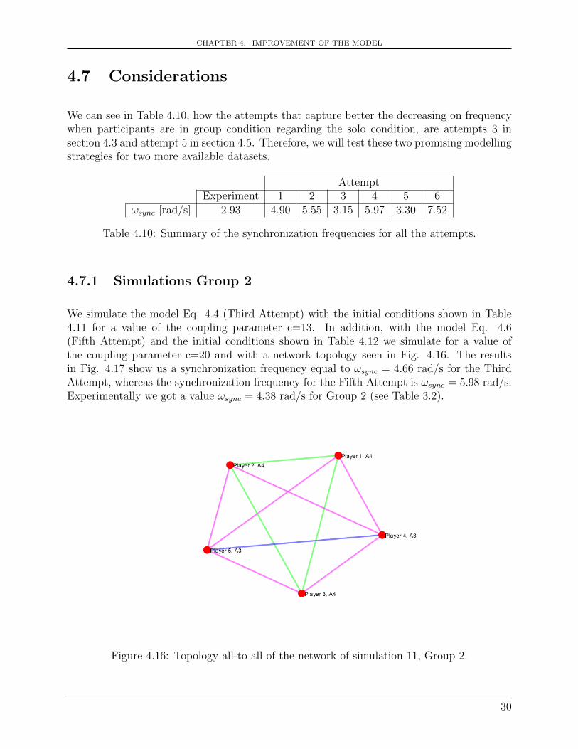
as follows: if the edge is blue players k and h share Attempt 3, if the edge is green players kand h share Attempt 4, if the edge is yellow player k follows Attempt 3 and player h followsAttempt 4 and finally if the edge is magenta player k follows Attempt 4 and player h followsAttempt 3 (see summary in Table 4.7). The results in Fig. 4.13 show us that synchronizationis achieved for a value of ωsync = 3.30 rad/s, a value close to the experimental one, and similarto the one get in the Third Attempt.

Color of the edgeBlue Green Yellow Magenta

Player k A3 A4 A3 A4Player h A3 A4 A4 A3

Table 4.7: Meaning of the colors in the figures of topologies. A3= Third Attempt, A4=Fourth Attempt.


Player 1 Player 2 Player 3 Player 4 Player 5ωk[rad/s] 1.98 3.18 6.82 3.37 8.51θk0[rad] -0.62 -0.96 -1.23 1.58 2.38


27



4.6 Sixth Attempt

In this last attempt, we exchange the strategies presented in the previous one. Now if thedeviation of an individual is higher than the mean deviation of the group, we define his links,using Attempt 3 (the player follows people more coherent with themselves). If the deviationof an individual is smaller than the mean deviation of the group, we define his links usingAttempt 4 (he follows people less coherent with themselves).

θk = wk + cN∑h=1

akhsin(θh − θk)

ifSDk >

1

N

∑Nk=1 SDK , akh =

SDk

SDh

∈ [0, 1]

ifSDk <1

N

∑Nk=1 SDK , akh =

SDh

SDk

∈ [0, 1](4.7)

In Fig. 4.14 we can see that synchronization is always achieved for a value c ≥ 18. Wesimulate the model Eq. 4.7 with the initial conditions shown in Table 4.9 for a value of thecoupling parameter c=18. The results in Fig. 4.15 show us synchronization is achieved for avalue of ωsync = 7.52 rad/s, a value indeed higher than the mean of the players in the solocondition.

28



Figure 4.14: Synchronization in Sixth Attempt, Group 1.

Player 1 Player 2 Player 3 Player 4 Player 5ωk[rad/s] 5.82 2.95 6.97 3.32 10.34θk0[rad] 1.31 -0.55 1.40 2.28 -0.02



29


4.7 Considerations

We can see in Table 4.10, how the attempts that capture better the decreasing on frequencywhen participants are in group condition regarding the solo condition, are attempts 3 insection 4.3 and attempt 5 in section 4.5. Therefore, we will test these two promising modellingstrategies for two more available datasets.

AttemptExperiment 1 2 3 4 5 6

ωsync [rad/s] 2.93 4.90 5.55 3.15 5.97 3.30 7.52

Table 4.10: Summary of the synchronization frequencies for all the attempts.

4.7.1 Simulations Group 2

We simulate the model Eq. 4.4 (Third Attempt) with the initial conditions shown in Table4.11 for a value of the coupling parameter c=13. In addition, with the model Eq. 4.6(Fifth Attempt) and the initial conditions shown in Table 4.12 we simulate for a value ofthe coupling parameter c=20 and with a network topology seen in Fig. 4.16. The resultsin Fig. 4.17 show us a synchronization frequency equal to ωsync = 4.66 rad/s for the ThirdAttempt, whereas the synchronization frequency for the Fifth Attempt is ωsync = 5.98 rad/s.Experimentally we got a value ωsync = 4.38 rad/s for Group 2 (see Table 3.2).


30


Player 1 Player 2 Player 3 Player 4 Player 5ωk[rad/s] 5.87 7.85 7.82 5.29 3.38θk0[rad] -1.51 -1.93 -0.92 -2.16 0.34

Table 4.11: Initial conditions for simulation 10. Third Attempt, Group 2.

Player 1 Player 2 Player 3 Player 4 Player 5ωk[rad/s] 6.41 7.04 7.37 5.07 3.50θk0[rad] 0.17 1.69 0.86 -1.29 1.65

Table 4.12: Initial conditions for simulation 11. Fifth Attempt, Group 2.

(a) Third attempt. ωsync = 4.66 rad/s. (b) Fifth Attempt. ωsync = 5.98 rad/s.

Figure 4.17: Simulations with dataset of Group 2. In (a) the frequency of each player withthe Third Attempt is represented, Simulation 10. In (b) the frequency of each player withthe Fifth Attempt is represented, Simulation 11.

4.7.2 Simulations Group 3

We simulate the model Eq. 4.4 (Third Attempt) with the initial conditions shown in Table4.13 for a value of the coupling parameter c=13. In addition with the model Eq. 4.6 (FifthAttempt) and the initial conditions shown in Table 4.14 we simulate for a value of the couplingparameter c=20 and with a network topology seen in Fig. 4.18. The results in Fig. 4.19show us a synchronization frequency ωsync = 2.72 rad/s for the Third Attempt, whereas thesynchronization frequency for the Fifth Attempt is ωsync = 2.54 rad/s. Experimentally wegot a value ωsync = 2.77 rad/s for Group 2 (see Table 3.2).

31


Player 1 Player 2 Player 3 Player 4 Player 5ωk[rad/s] 2.62 2.82 2.84 2.34 2.72θk0[rad] -0.06 -0.34 0.92 1.31 1.60

Table 4.13: Initial conditions for simulation 12. Third Attempt, Group 3.

Player 1 Player 2 Player 3 Player 4 Player 5ωk[rad/s] 2.43 2.87 2.58 2.00 2.90θk0[rad] 2.89 -1.00 0.53 -1.73 1.58

Table 4.14: Initial conditions for simulation 13. Fifth Attempt, Group 3.


32


(a) Third attempt. ωsync = 2.72 rad/s. (b) Fifth Attempt. ωsync = 2.54 rad/s.

(c) Detail of the first 2 seconds. (d) Detail of the first 2 seconds.

Figure 4.19: Simulations with dataset of Group 3. In (a) and (c) is represented the frequencyof each player with the Third Attempt, Simulation 12. In (b) and (d) and is represented thefrequency of each player with the Fifth Attempt, Simulation 13.

4.7.3 Summary

To sum up, we have seen that for Group 1, Third Attempt and Fifth Attempt are the onesthat reproduce better experimental results, so we have computed again both for differentdata sets obtained experimentally. In Group 2, the Third Attempt replicates better theexperiments, and Fifth Attempt is further from the value we are trying to capture. Finally,in Group 3, both attempts seem to work well, but if we look at Table 3.1 we can see how thevariability of the frequencies in solo condition is very small, as a result, players do not needto interact between them to reach synchronization because at the beginning they are alreadyalmost synchronized.

33

Chapter 5

Conclusions

We have seen how important is synchronization in human ensembles as well as in nature, forinstance in physics, biology and chemistry. In chapter 2 a model to represent synchronizationin a group of oscillators has been described, the Kuramoto’s Model, in addition to twodifferent types of synchronization, the phase-locking and the phase-synchronization and aeffective way to measure them. After, in chapter 3 we have seen the setup and experimentaldata get in the experiments run in Naples in December 2017, from which a decrease insynchronization frequency has been observed regarding the mean natural frequencies of theplayers taking part in the experiment. Moreover, it has been attempted to reproduce thesehuman interactions as a network of Kuramoto’s oscillators with the limitations to which ithas given rise. Finally, in chapter 4 we have tried to overcome these limitations, modifyingthe Kuramoto’s Model. Six different attempts have been computed focus on them fromdifferent points of view. We have seen how some of them, in particular Attempts 1,2,4and 6 do not work as we expected, whereas Attempts 3 and 5 reproduced quite well theexperimental result got with the first group of the three who participated in the experiments.However, computing these two promising attempts for the other groups, we have seen thatthe Fifth Attempt is further from the experimental synchronization frequency in Group 2and the Third Attempt reproduced the experimental results for all the groups. Therefore, itis considered that the Third Attempt is the best adaptation to the Kuramoto’s model ableto represent the behaviour of people when they have to synchronize to perform a joint taskas the one carried out in the experiment of this work.

The work presented in this thesis has many possible future improvements and developments.It can be tried to improve the Third Attempt to get a more precise value to the experimentalone. Furthermore, due to the synchronization frequency of the Third Attempt depends inparticular on the intrinsic definition of each individual of the group, it could be possible todo a previous personality study of the group members taking part on the experiment to knowhow they affect the dynamics and in particular the linkage between players.

Bibliography

[1] Steven H. Strogatz. From kuramoto to crawford: exploring the onset of synchronizationin populations of coupled oscillators. Physica D: Nonlinear Phenomena, 143(1):1 – 20,2000.

[2] Manuel Varlet, Ludovic Marin, Delphine Capdevielle, Jonathan Del-Monte, RichardSchmidt, Robin Salesse, Jean-Philippe Boulenger, Benoıt Gael Bardy, and StephaneRaffard. Difficulty leading interpersonal coordination: towards an embodied signatureof social anxiety disorder. Frontiers in behavioral neuroscience, 8:29, 2014.

[3] Jonathan Del-Monte, Delphine Capdevielle, Manuel Varlet, Ludovic Marin, RichardSchmidt, Robin Salesse, Benoıt Bardy, jean-Philippe Boulenger, Marie Christine Gely-Nargeot, Jerome Attal, and Stephane Raffard. Social motor coordination in unaffectedrelatives of schizophrenia patients: A potential intermediate phenotype. Frontiers inBehavioral Neuroscience, 7:137, 2013.

[4] Chao Zhai, Francesco Alderisio, Krasimira Tsaneva-Atanasova, and Mario Di Bernardo.A novel cognitive architecture for a human-like virtual player in the mirror game. volume2014, 10 2014.

[5] Mathworks.com. (2019). MATLAB MathWorks. [online] Available at:https://www.mathworks.com/products/matlab.html.

[6] Yoshiki (1975). H. Araki Kuramoto. Ed. Lecture Notes In Physics, International Sympo-sium On Mathematical Problems In Theoretical Physics. 39. Springer-verlag, New York.P. 420.

[7] Rick B. van Baaren, Rob W. Holland, Kerry Kawakami, and Ad van Knippenberg.Mimicry and prosocial behavior. Psychological Science, 15(1):71–74, 2004. PMID:14717835.

[8] Olivier Oullier, Gonzalo C. de Guzman, Kelly J. Jantzen, Julien Lagarde, and J. A. ScottKelso. Social coordination dynamics: measuring human bonding. Social neuroscience,3(18552971):178–192, June 2008.

[9] R. C. Schmidt and M. T. Turvey. Phase-entrainment dynamics of visually coupledrhythmic movements. Biological Cybernetics, 70(4):369–376, Feb 1994.

BIBLIOGRAPHY

[10] Iain D. Couzin, Jens Krause, Nigel R. Franks, and Simon A. Levin. Effective leadershipand decision-making in animal groups on the move. Nature, 433:513, February 2005.

[11] Mate Nagy, Zsuzsa Akos, Dora Biro, and Tamas Vicsek. Hierarchical group dynamicsin pigeon flocks. Nature, 464:890, April 2010.

[12] T.D. Frank and M.J. Richardson. On a test statistic for the kuramoto order parameterof synchronization: An illustration for group synchronization during rocking chairs.Physica D: Nonlinear Phenomena, 239(23):2084 – 2092, 2010.

[13] T. Iqbal and L. D. Riek. A method for automatic detection of psychomotor entrainment.IEEE Transactions on Affective Computing, 7(1):3–16, Jan 2016.

[14] Erwan Codrons, Nicolo F. Bernardi, Matteo Vandoni, and Luciano Bernardi. Spon-taneous group synchronization of movements and respiratory rhythms. PLOS ONE,9(9):1–10, 09 2014.

[15] Alan Wing and Charles Woodburn. The coordination and consistency of rowers in aracing eight. Journal of sports sciences, 13:187–97, 07 1995.

[16] Keiko Yokoyama and Yuji Yamamoto. Three people can synchronize as coupled oscilla-tors during sports activities. PLOS Computational Biology, 7(10):1–8, 10 2011.

[17] Chao Zhai, Michael Z. Q. Chen, Francesco Alderisio, Alexei Uteshev, and MarioDi Bernardo. An interactive control architecture for interpersonal coordination in mirrorgame. Control Engineering Practice, 80:36–48, 08 2018.

[18] Alessandro D’Ausilio, Leonardo Badino, Yi Li, Sera Tokay, Laila Craighero, RosarioCanto, Yiannis Aloimonos, and Luciano Fadiga. Leadership in orchestra emerges fromthe causal relationships of movement kinematics. PLOS ONE, 7(5):1–6, 05 2012.

[19] Francesco Alderisio, Gianfranco Fiore, Robin N Salesse, Benoit G Bardy, and Mariodi Bernardo. Interaction patterns and individual dynamics shape the way we move insynchrony.

[20] Juan Acebron, Luis Bonilla, Conrado Perez-Vicente, Felix Ritort Farran, and RenatoSpigler. The kuramoto model: A simple paradigm for synchronization phenomena.Reviews of Modern Physics, 77, 04 2005.

[21] Florian Dorfler and Francesco Bullo. Transient Stability Analysis in Power Net-works and Synchronization of Non-uniform Kuramoto Oscillators. Technical ReportarXiv:0910.5673, Oct 2009.

[22] Rodolphe Sepulchre, Derek Paley, and Naomi Leonard. Collective motion and oscillatorsynchronization. In Cooperative control, pages 189–205. Springer, 2005.

[23] Complexity-explorables.org. (2019). Ride my Kuramotocycle!. [online] Available at:http://www.complexity-explorables.org/explorables/kuramoto/.

36

BIBLIOGRAPHY

[24] Francesco Alderisio, Maria Lombardi, Gianfranco Fiore, and Mario di Bernardo. A novelcomputer-based set-up to study movement coordination in human ensembles. Frontiersin Psychology, 8:967, 2017.

[25] Dibernardogroup.github.io. (2019). Chronos. [online] Available at:https://dibernardogroup.github.io/Chronos/.

[26] Leap Motion. (2019). Leap Motion. [online] Available at: https://www.leapmotion.com/.

[27] Bjorn Kralemann, Laura Cimponeriu, Michael Rosenblum, Arkady Pikovsky, and RalfMrowka. Phase dynamics of coupled oscillators reconstructed from data. Physical review.E, Statistical, nonlinear, and soft matter physics, 77:066205, 06 2008.

[28] B. Boashash. , ed. (2003), Time-Frequency Signal Analysis and Processing: A Compre-hensive Reference, Oxford: Elsevier Science, ISBN 978-0-08-044335-5.

37

modeling human interactions as a network of kuramoto’s

Documents