TECHNICAL PAPER

Modeling Flexible Bodies with Simscape Multibody SoftwareAn Overview of Two Methods for Capturing the Effects of Small Elastic Deformations

By S. Miller, T. Soares, Y. Van Weddingen, and J. Wendlandt

Contents

1 Introduction 11.1 Why Model Flexible Bodies? . . . . . . . . . . . . . . . . . . . . . . . . . . . . . . . . . . . . 11.2 Two Modeling Approaches . . . . . . . . . . . . . . . . . . . . . . . . . . . . . . . . . . . . . . 11.3 The Scope of This Paper . . . . . . . . . . . . . . . . . . . . . . . . . . . . . . . . . . . . . . . 2

2 Lumped-Parameter Method 22.1 Overview . . . . . . . . . . . . . . . . . . . . . . . . . . . . . . . . . . . . . . . . . . . . . . . 22.2 Method . . . . . . . . . . . . . . . . . . . . . . . . . . . . . . . . . . . . . . . . . . . . . . . . 3

2.2.1 Step 1: Model the Mass Elements that Comprise the Body . . . . . . . . . . . . . . . 32.3 Theory . . . . . . . . . . . . . . . . . . . . . . . . . . . . . . . . . . . . . . . . . . . . . . . . . 4

2.3.1 Harmonic Oscillators . . . . . . . . . . . . . . . . . . . . . . . . . . . . . . . . . . . . . 42.3.2 Spring Coefficient . . . . . . . . . . . . . . . . . . . . . . . . . . . . . . . . . . . . . . 52.3.3 Damping Coefficient . . . . . . . . . . . . . . . . . . . . . . . . . . . . . . . . . . . . . 6

2.4 Examples . . . . . . . . . . . . . . . . . . . . . . . . . . . . . . . . . . . . . . . . . . . . . . . 72.4.1 Flexible Cantilever Beam . . . . . . . . . . . . . . . . . . . . . . . . . . . . . . . . . . 72.4.2 Crank-Slider with Flexible Links . . . . . . . . . . . . . . . . . . . . . . . . . . . . . . 10

3 Finite-Element Import Method 163.1 Overview . . . . . . . . . . . . . . . . . . . . . . . . . . . . . . . . . . . . . . . . . . . . . . . 16

3.1.1 Deformation Model . . . . . . . . . . . . . . . . . . . . . . . . . . . . . . . . . . . . . . 173.1.2 Interface Frames . . . . . . . . . . . . . . . . . . . . . . . . . . . . . . . . . . . . . . . 183.1.3 Deflection Joints . . . . . . . . . . . . . . . . . . . . . . . . . . . . . . . . . . . . . . . 183.1.4 Reference Frame . . . . . . . . . . . . . . . . . . . . . . . . . . . . . . . . . . . . . . . 19

3.2 Method . . . . . . . . . . . . . . . . . . . . . . . . . . . . . . . . . . . . . . . . . . . . . . . . 193.3 Guidelines . . . . . . . . . . . . . . . . . . . . . . . . . . . . . . . . . . . . . . . . . . . . . . . 22

3.3.1 Algebraic Loops . . . . . . . . . . . . . . . . . . . . . . . . . . . . . . . . . . . . . . . 223.3.2 Interface Inertias . . . . . . . . . . . . . . . . . . . . . . . . . . . . . . . . . . . . . . . 233.3.3 Body Visualization . . . . . . . . . . . . . . . . . . . . . . . . . . . . . . . . . . . . . . 24

3.4 Theory . . . . . . . . . . . . . . . . . . . . . . . . . . . . . . . . . . . . . . . . . . . . . . . . . 243.4.1 Model Reduction . . . . . . . . . . . . . . . . . . . . . . . . . . . . . . . . . . . . . . . 253.4.2 Rigid-Body Modes . . . . . . . . . . . . . . . . . . . . . . . . . . . . . . . . . . . . . . 273.4.3 Modal Damping . . . . . . . . . . . . . . . . . . . . . . . . . . . . . . . . . . . . . . . 283.4.4 State-Space System . . . . . . . . . . . . . . . . . . . . . . . . . . . . . . . . . . . . . 29

3.5 Examples . . . . . . . . . . . . . . . . . . . . . . . . . . . . . . . . . . . . . . . . . . . . . . . 303.5.1 Flexible Cantilever Beam . . . . . . . . . . . . . . . . . . . . . . . . . . . . . . . . . . 303.5.2 Crank-Slider with Flexible Links . . . . . . . . . . . . . . . . . . . . . . . . . . . . . . 31

4 Conclusion 36

1 Introduction

1.1 Why Model Flexible Bodies?

The assumption is often made in the construction of a multibody model that bodies do not deform. Eachbody is treated as a rigid unit, incapable of the mechanically induced distortions that real, and morecompliant, materials frequently experience. The rigid-body approximation suits a wide array of multibodymodels. It is simple, allowing for faster simulation. It is also, in many applications, amply accurate: thematerial and geometry of a body are often specified so that the body does not appreciably deform.

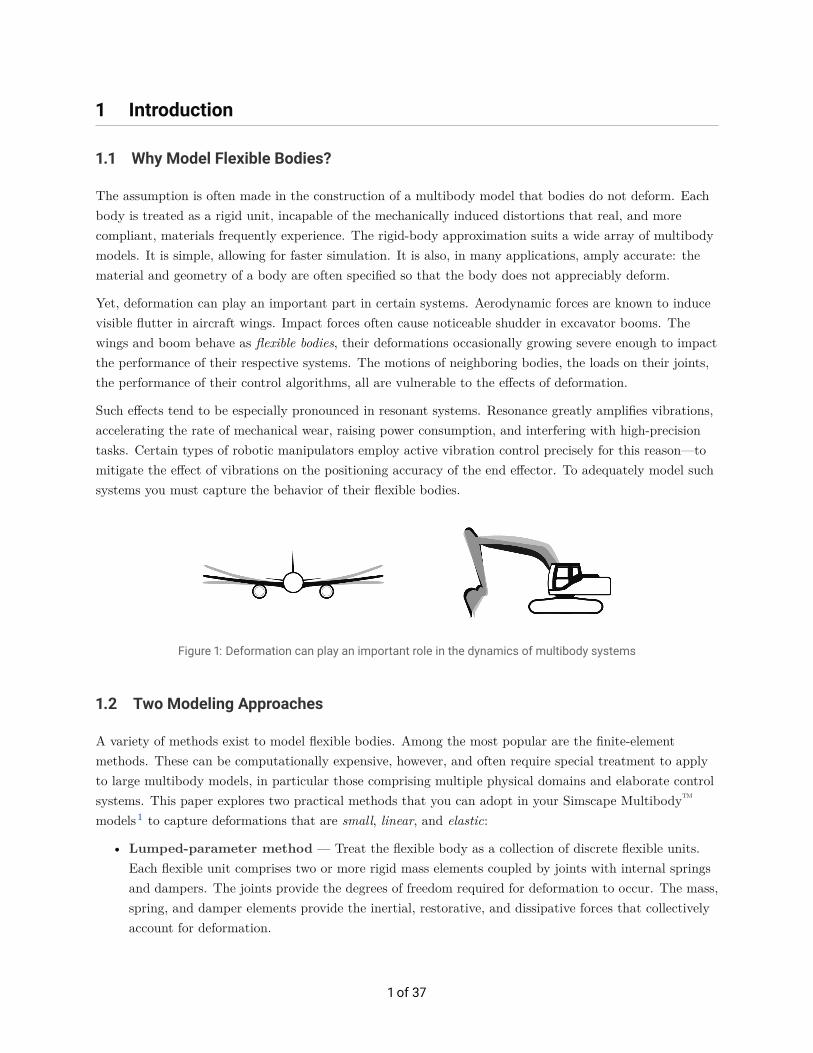
Yet, deformation can play an important part in certain systems. Aerodynamic forces are known to inducevisible flutter in aircraft wings. Impact forces often cause noticeable shudder in excavator booms. Thewings and boom behave as flexible bodies, their deformations occasionally growing severe enough to impactthe performance of their respective systems. The motions of neighboring bodies, the loads on their joints,the performance of their control algorithms, all are vulnerable to the effects of deformation.

Such effects tend to be especially pronounced in resonant systems. Resonance greatly amplifies vibrations,accelerating the rate of mechanical wear, raising power consumption, and interfering with high-precisiontasks. Certain types of robotic manipulators employ active vibration control precisely for this reason—tomitigate the effect of vibrations on the positioning accuracy of the end effector. To adequately model suchsystems you must capture the behavior of their flexible bodies.

Figure 1: Deformation can play an important role in the dynamics of multibody systems

1.2 Two Modeling Approaches

A variety of methods exist to model flexible bodies. Among the most popular are the finite-elementmethods. These can be computationally expensive, however, and often require special treatment to applyto large multibody models, in particular those comprising multiple physical domains and elaborate controlsystems. This paper explores two practical methods that you can adopt in your Simscape Multibody™

models1 to capture deformations that are small, linear, and elastic:

• Lumped-parameter method — Treat the flexible body as a collection of discrete flexible units.Each flexible unit comprises two or more rigid mass elements coupled by joints with internal springsand dampers. The joints provide the degrees of freedom required for deformation to occur. The mass,spring, and damper elements provide the inertial, restorative, and dissipative forces that collectivelyaccount for deformation.

1 of 37

• Finite-element import method — Treat the flexible body as the superposition of distinctrigid-body and deformation models. The rigid-body model captures the motion of the body asthough it were incapable of deforming. The deformation model captures the deflections within thebody as though it were fixed in place. The method derives its name from the source of much of thedata behind the deformation model: a finite-element model.

1.3 The Scope of This Paper

The discussion presented here details each method, with special attention given to its workflow andparameter calculations. Some familiarity with multibody modeling is assumed. Two modeling examples arediscussed—one a cantilever beam under point and distributed loads, the other a crank-slider mechanismwith and without contact forces. The simulation results obtained from each method are compared toanalytical predictions or, when these are unavailable, to relevant results from the scientific literature.

2 Lumped-Parameter Method

2.1 Overview

The lumped-parameter method approximates a flexible body as a collection of discrete flexible units fixedto one another. In the simple case of a long slender body, a flexible unit comprises two mass elementscoupled with a joint possessing internal springs and dampers. The degrees of freedom of the joint capturethe deformation modes of the flexible unit. The springs and dampers capture its stiffness and dampingcharacteristics.

This method suits bodies with slender geometries, such as rods and beams. Figure 2 shows a simpleexample: a beam discretized along its length into four flexible beam units. The shaded area highlights oneflexible unit. Within it are the two mass elements (m), the spring (k), and the damper (b) common to allflexible units. Rigid connections join the flexible units to their respective neighbors.

Figure 2: A flexible body according to the lumped-parameter method

2 of 37

2.2 Method

The lumped-parameter method comprises the four steps described below. For more information on how toperform a specific task in a Simscape Multibody model, see the Simscape Multibody documentation.Examples of multibody models based on the lumped-parameter method are available for download fromthe MATLAB Central™ File Exchange website.

2.2.1 Step 1: Model the Mass Elements that Comprise the Body

Each mass element accounts for a small section of the body. All are assumed rigid. The accuracy of thelumped-parameter method depends in part on the number of mass elements used. Increasing this numbertends to improve the accuracy attained (albeit at a greater computational cost). In the figure, each squarecorresponds to a mass element.

Step 2: Connect the Mass Elements in Pairs with Joints

Each mass-joint-mass sequence represents a flexible body unit. The joints provide the degrees of freedomcorresponding to the different types of deformation. Rotational degrees of freedom enable bending andtorsion. Translational degrees of freedom enable axial deformation and shear. If bending is considered, thejoint must lie on the neutral axis of the body.

Step 3: Add Springs and Dampers to the Various Joints

The spring and damping coefficients determine the static and dynamic deformations arising from appliedforces and torques. You must calculate these coefficients from knowledge of the geometry and materialproperties of the beam. The calculations are outlined in sections 2.3.2 and 2.3.3.

3 of 37

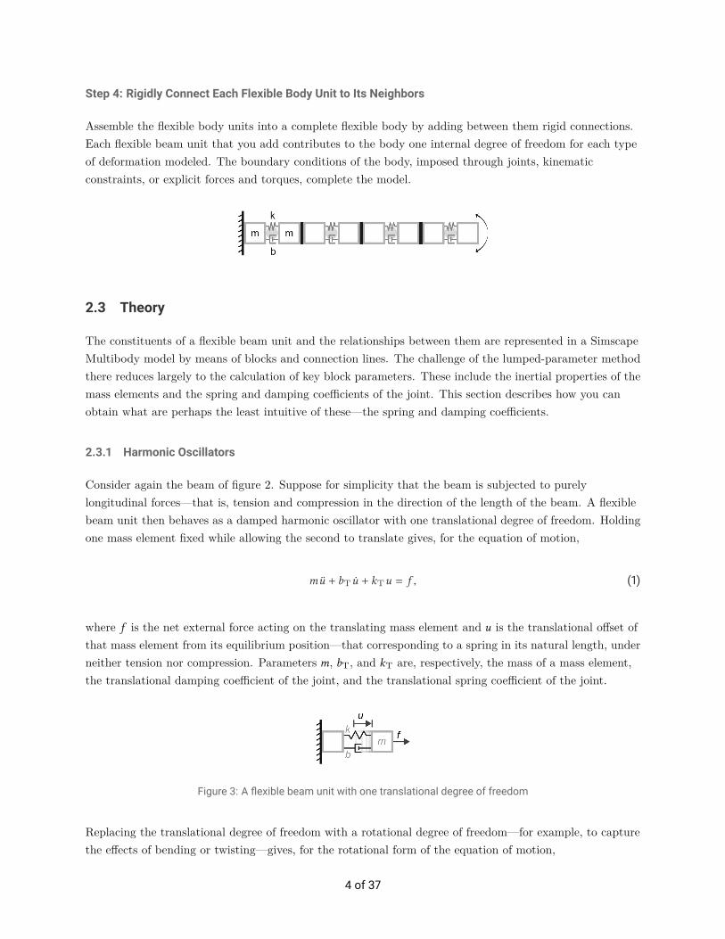
Step 4: Rigidly Connect Each Flexible Body Unit to Its Neighbors

Assemble the flexible body units into a complete flexible body by adding between them rigid connections.Each flexible beam unit that you add contributes to the body one internal degree of freedom for each typeof deformation modeled. The boundary conditions of the body, imposed through joints, kinematicconstraints, or explicit forces and torques, complete the model.

2.3 Theory

The constituents of a flexible beam unit and the relationships between them are represented in a SimscapeMultibody model by means of blocks and connection lines. The challenge of the lumped-parameter methodthere reduces largely to the calculation of key block parameters. These include the inertial properties of themass elements and the spring and damping coefficients of the joint. This section describes how you canobtain what are perhaps the least intuitive of these—the spring and damping coefficients.

2.3.1 Harmonic Oscillators

Consider again the beam of figure 2. Suppose for simplicity that the beam is subjected to purelylongitudinal forces—that is, tension and compression in the direction of the length of the beam. A flexiblebeam unit then behaves as a damped harmonic oscillator with one translational degree of freedom. Holdingone mass element fixed while allowing the second to translate gives, for the equation of motion,

m Üu + bT Ûu + kTu = f , (1)

where f is the net external force acting on the translating mass element and u is the translational offset ofthat mass element from its equilibrium position—that corresponding to a spring in its natural length, underneither tension nor compression. Parameters m, bT, and kT are, respectively, the mass of a mass element,the translational damping coefficient of the joint, and the translational spring coefficient of the joint.

Figure 3: A flexible beam unit with one translational degree of freedom

Replacing the translational degree of freedom with a rotational degree of freedom—for example, to capturethe effects of bending or twisting—gives, for the rotational form of the equation of motion,

4 of 37

I Üθ + bR Ûθ + kRθ = τ , (2)

where τ is the net external torque acting on the rotating mass element and θ is the rotational offset of thatmass element from its equilibrium position. Parameters I , bR, and kR are, respectively, the moment ofinertia of a mass element about the axis of rotation, the rotational damping coefficient of the joint, and therotational spring coefficient of the joint.

Expressing the rotational equation in terms of the often used damping ratio (ζ ) and natural frequency (ω)parameters gives

I(Üθ + 2ζ ω Ûθ + ω2θ

)= τ , (3)

where

ζ =bR

2√I kR

and ω =

√kRI. (4)

The damping ratio is simply the fraction of the true damping coefficient, bR, over the critical dampingcoefficient, 2

√IkR, the value at which the oscillator transitions between underdamped and overdamped

conditions. The natural frequency is the rate at which an undamped oscillator tends to vibrate in theabsence of an applied load. An isolated oscillator has one natural frequency. A complete flexible beam, as acomposite of harmonic oscillators, has many—one for each degree of freedom provided by the joints. In theexamples of section 2.4, the first four of these provide a benchmark by which to judge simulation results.

2.3.2 Spring Coefficient

In a cantilever beam subjected only to bending, the value of the spring coefficient follows from the equalitybetween the spring torque at the joint and the bending moment on a continuous version of the flexiblebeam unit. Hooke’s law gives the spring torque at the joint:

τk = kR θ , (5)

where τk is the spring torque, kR is the rotational spring constant, and θ is the deflection angle. Classicalbeam theory gives the bending moment on a continuous beam unit:

M =E IAR, (6)

5 of 37

where M is the bending moment, E is Young’s modulus of elasticity, IA is the second moment of area, and R

is the bending radius of curvature. In the limit of very small deflections, θ reduces to l/R, where l is theundeformed length of a flexible beam unit, and the spring coefficient becomes

kR =E IAl. (7)

If the flexible beam has length L and a number N of flexible beam units, then the length l of anundeformed flexible beam unit is simply

l =L

N. (8)

Figure 4 shows the angle (θ) and radius of curvature (R) due to bending. A mass element is half the lengthof a flexible beam unit, l/2.

Figure 4: Geometry of a flexible beam unit with one rotational degree of freedom

The spring coefficients corresponding to other deformation types follow from a similar analysis. Table 1summarizes the cases of axial and torsional deformation. Here, ϕ and δ are the torsional and axialdeformations, kT and kA the torsional and axial spring constants, and G, J , and A the shear modulus,torsional constant, and cross-sectional area of the beam.

Deformation Mode Hooke’s Law Elasticity Theory Spring Coefficient

Torsional τk = kT ϕ M = G Jϕ/l kT = G J/l

Axial fk = kA δ F = EAδ/l kA = EA/l

Table 1: Joint spring coefficients

2.3.3 Damping Coefficient

The damping of materials is a complex phenomenon and often a challenge to characterize accurately.Sophisticated damping models exist but here a simple one is chosen. Let damping be linear and bound by

6 of 37

a constitutive law of the type

τb = bR Ûθ , (9)

where τk is the magnitude of the damping torque between two mass elements connected with one rotationaldegree of freedom. This assumption is consistent with the damping calculations of the Simscape Multibodyjoint blocks. As a first-order approximation, take the damping coefficient to be proportional to the springcoefficient:

bR = αkR (10)

The proportionality constant (α) is an empirically set damping factor. The damping coefficient then scalesdirectly with the discretization level of the beam: increase the number of flexible beam units and thedamping coefficient increases also. This scaling is provided by the spring coefficient as calculated inequations 7 and 8.

The damping factor can be set by matching the lumped-parameter deformations to reliable benchmarkdata. The calculated deformations should closely mirror those determined by experiment or by thesimulation of a trusted model of the same body.

2.4 Examples

2.4.1 Flexible Cantilever Beam

Consider a lumped-parameter model of an aluminum cantilever beam under two loading conditions: one adistributed load provided by gravity, the other an upward point force of 20 N applied at the free end of thebeam in zero gravity (see figure 5). This model is available for download from the MATLAB® Central FileExchange. For the clear visualization of beam deformation in the distributed load case, the gravitationalacceleration (д) is set there to an artificially high value of -981 m/s2.

Beam Properties Table 2 summarizes the properties of the beam. The beam is approximately one foot inlength and half an inch in width. Its construction is of aluminum. Its second moment of area is calculatedfrom the standard analytical expression for a rectangular cross section:

IA =WT 3

12. (11)

7 of 37

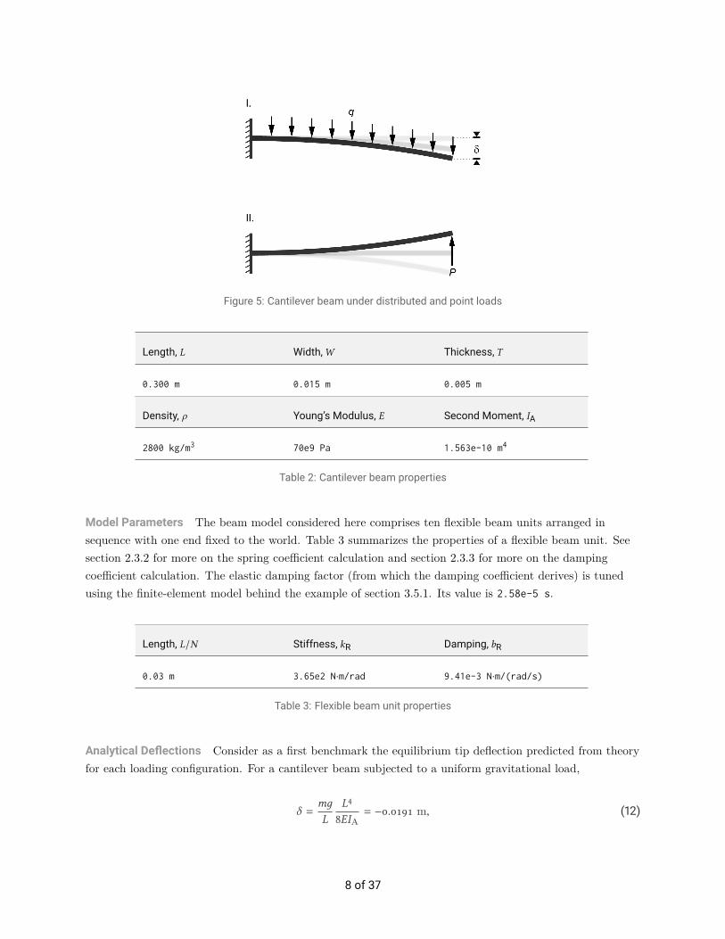
Figure 5: Cantilever beam under distributed and point loads

Length, L Width,W Thickness, T

0.300 m 0.015 m 0.005 m

Density, ρ Young’s Modulus, E Second Moment, IA

2800 kg/m3 70e9 Pa 1.563e-10 m4

Table 2: Cantilever beam properties

Model Parameters The beam model considered here comprises ten flexible beam units arranged insequence with one end fixed to the world. Table 3 summarizes the properties of a flexible beam unit. Seesection 2.3.2 for more on the spring coefficient calculation and section 2.3.3 for more on the dampingcoefficient calculation. The elastic damping factor (from which the damping coefficient derives) is tunedusing the finite-element model behind the example of section 3.5.1. Its value is 2.58e-5 s.

Length, L/N Stiffness, kR Damping, bR

0.03 m 3.65e2 N·m/rad 9.41e-3 N·m/(rad/s)

Table 3: Flexible beam unit properties

Analytical Deflections Consider as a first benchmark the equilibrium tip deflection predicted from theoryfor each loading configuration. For a cantilever beam subjected to a uniform gravitational load,

δ =mд

L

L4

8EIA= −0.0191 m, (12)

8 of 37

where the term mдL is the gravitational force acting on a unit length of the beam under the assumption that

д = −981 m/s2. For a cantilever beam subjected to a point force applied at the tip in a zero-gravityenvironment,

δ =PL3

3EIA= 0.0165 m, (13)

where P is the point force, chosen here to have a magnitude of 20 N.

Analytical Frequencies Consider as a second benchmark the set of natural frequencies ωi predicted fromtheory for the cantilever beam in the undamped, unloaded case:

ωi =(αiL

)2√

EIAρA, (14)

where i are the indices of the free vibration modes and αi the multipliers specific to those modes, defined asthe ith roots of the transcendental equation

1 + cos (α) cosh (α) = 0. (15)

For a cantilever beam, the first four values of αi are 1.875, 4.694, 7.855, and 10.996, yielding, for the firstfour modes, the natural frequencies

ωI = 281.91 rad/s, ωII = 1766.82 rad/s, ωIII = 4947.65 rad/s, ωIV = 9695.64 rad/s.

In units of Hertz (using the equality fi = ωi/2π),

fI = 44.87 Hz, fII = 281.20 Hz, fIII = 787.44 Hz, fIV = 1543.11 Hz.

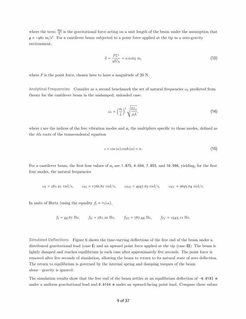
Simulated Deflections Figure 6 shows the time-varying deflections of the free end of the beam under adistributed gravitational load (case I) and an upward point force applied at the tip (case II). The beam islightly damped and reaches equilibrium in each case after approximately five seconds. The point force isremoved after five seconds of simulation, allowing the beam to return to its natural state of zero deflection.The return to equilibrium is governed by the internal spring and damping torques of the beamalone—gravity is ignored.

The simulation results show that the free end of the beam settles at an equilibrium deflection of -0.0183 m

under a uniform gravitational load and 0.0164 m under an upward-facing point load. Compare these values

9 of 37

to the analytical predictions of -0.0191 m for a uniform gravitational load and 0.0165 m for anupward-facing point load, respectively.

Figure 6: Tip deflection due to a distributed gravitational load (left) and to an upward point load (right)

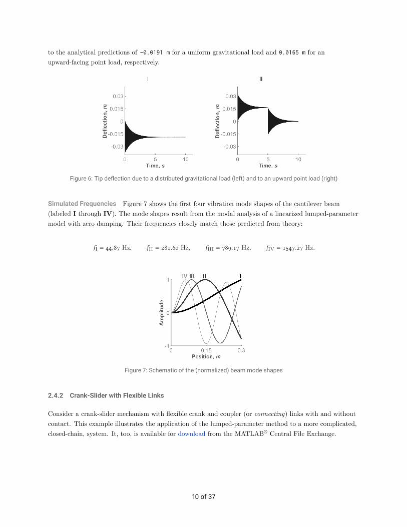
Simulated Frequencies Figure 7 shows the first four vibration mode shapes of the cantilever beam(labeled I through IV). The mode shapes result from the modal analysis of a linearized lumped-parametermodel with zero damping. Their frequencies closely match those predicted from theory:

fI = 44.87 Hz, fII = 281.60 Hz, fIII = 789.17 Hz, fIV = 1547.27 Hz.

Figure 7: Schematic of the (normalized) beam mode shapes

2.4.2 Crank-Slider with Flexible Links

Consider a crank-slider mechanism with flexible crank and coupler (or connecting) links with and withoutcontact. This example illustrates the application of the lumped-parameter method to a more complicated,closed-chain, system. It, too, is available for download from the MATLAB® Central File Exchange.

10 of 37

Figure 8: Crank-slider mechanism with flexible crank (A) and coupler (B) links

For comparison purposes, the model is configured with the material and geometry properties described in acase study published by A. Shabana2. The crank shaft is driven by an applied torque of the form

M(t) =

0.01

(1 − e

−t0.167

)t < 0.70s

0 t ≥ 0.70s, (16)

Figure 9: Driving torque applied at the crank joint

Link Properties Table 4 summarizes the properties of the crank and coupler links. The coupler isapproximately one foot in length and the crank half a foot. The links have the same cross-sectionalgeometry and density but different moduli of elasticity, with the crank being just over one order ofmagnitude stiffer than the coupler.

11 of 37

Link Length, L Width,W Thickness, T

Crank 0.152 m 0.0091 m 0.0087 m

Coupler 0.304 m 0.0091 m 0.0087 m

Link Density, ρ Young’s Modulus, E Second Moment, IA

Crank 2770 kg/m3 1e9 Pa 4.909e-10 m4

Coupler 2770 kg/m3 5e7 Pa 4.909e-10 m4

Table 4: Crank and coupler link properties

Model Parameters The crank and coupler are modeled as flexible beams each rectangular in crosssection. The crank comprises ten flexible beam units and the coupler twenty. The flexible beam units haveone rotational degree of freedom each, about an axis that is simultaneously perpendicular to the (vertical)gravity vector and to the (horizontal) path of the slider.

Table 5 summarizes the properties of an individual flexible beam unit. See section 2.3.2 for more on thespring coefficient calculation and section 2.3.3 for more on the damping coefficient calculation. The elasticdamping factors (from which the damping coefficients derive) are tuned using the finite-element modelbehind the examples of section 3.5.2. Their values are 3.38e-5 s for the crank and 6.03e-4 s for thecoupler.

Link Length, L/N Stiffness, kR Damping, bR

Crank 0.0152 m 32.30 N·m/rad 1.09e-3 N·m/(rad/s)

Coupler 0.0152 m 1.61 N·m/rad 9.74e-4 N·m/(rad/s)

Table 5: Flexible beam unit properties

Simscape Multibody Model Figure 10 shows a Simscape Multibody model of the crank-slider mechanism.The crank and coupler are both modeled using the lumped-parameter method. The various bodies connectto each other and to the world by means of joints. The driving torque is applied directly to the world-crankrevolute joint and the hard-stop force is applied directly to the slider-world prismatic joint.

12 of 37

Figure 10: Simscape Multibody model of a crank-slider mechanism

Figure 11 shows a Simscape Multibody model of one flexible body—the coupler. For simplicity, the modelis shown with only four flexible beam units. These are each enclosed in a Simulink Subsystem block (namedFlexible Unit 1–4). Two Rigid Transform blocks (Rigid Transform A–B) define the placement of theconnection frames (B and F) of the body—those through which it connects to the remainder of the model.

Figure 11: Simscape Multibody model of a flexible coupler

Within each flexible beam unit are additional blocks representing its constituent components. Two Solidblocks (named Mass 1–2) represent the mass elements of the flexible beam unit. They are connected by aRevolute Joint block (Joint) within which are the spring and the damper needed to capture compliantbehavior. The properties of the flexible beam unit are specified as parameters of these blocks.

Figure 12: Simscape Multibody model of a flexible beam unit

The four Rigid Transform blocks (Rigid Transform 1A–2B) merely define the placement of the various

13 of 37

connection frames—those through which the mass elements connect to each other and those through whichthe flexible beam unit connects to its neighbors.

Simulated Deflections Figure 13 overlays the simulation results obtained using the lumped-parametermethod (curve B) on those published by A. Shabana (curve A). The curves each correspond to thetransverse deflection measured at the midpoint of the coupler link with respect to an imaginary line drawnbetween the longitudinal ends of the same link.

Figure 13: Comparison to Shabana 2 simulation results (A: Shabana, B: Simscape Multibody)

Figure 14 shows the simulation results obtained from a model with an obstacle—a translational hardstop—placed in the path of the slider. Contact occurs shortly after the 0.5-second mark, inducing in thecoupler link the vibrations shown. As before, the results correspond to the transverse deflection measuredat the midpoint of the coupler link. The oscillations decay at a rate determined by the damping coefficientused in the model.

Figure 14: Coupler deflection due to contact

Simulation Accuracy The simulation results depend closely on the number of flexible beam units used inthe model. Figure 15 compares the simulation results, in a model without an obstacle, for different crankand coupler discretizations. Curves A, B, C, and D correspond, respectively, to a crank with two, five,ten, and twenty flexible beam units and to a coupler with four, ten, twenty, and forty.

14 of 37

The simulated deflections approach those obtained by A. Shabana as the crank and coupler become morefinely discretized. At twenty flexible beam units in the crank and forty in the coupler only a smalldiscrepancy remains. This discrepancy may reflect a failure by the lumped-parameter method to preciselycapture the instantaneous curvature of the beam (upon which the bending moment depends). The resultspublished by A. Shabana are overlaid in bold (beneath curve D).

Figure 15: Effect of changing the level of discretization of the flexible bodies (A: 4-element coupler, B: 10-element coupler,C: 20-element coupler, D: 40-element coupler)

Visualization Results Figure 16 shows the visualization results obtained from a Simscape Multibodymodel of the crank-slider mechanism. The coupler is modeled as a rigid body in case I, as a flexible bodywith two flexible beam units in case II, and as a flexible body with ten flexible beam units in case III. Ineach case, the model is shown as it appears an instant (0.05 s) after collision with the hard stop.

Figure 16: Simscape Multibody visualization results for the lumped-parameter method (I: rigid coupler, II: 2-elementflexible coupler, III: 10-element flexible coupler)

The coupler is naturally undeformed in case I. It is slightly deformed in case II but, due to the smallnumber of flexible beam units, its visualization is rough in appearance. The same deformation is evident incase III, now with smoother visualization results produced by the greater number of flexible beam units.

15 of 37

3 Finite-Element Import Method

3.1 Overview

The finite-element import method approximates a flexible body as the superposition of a rigid-body modeland a deformation model (their motions shown in figure 17). The rigid-body model captures the rotationand translation of the body as if it did not deform at all. It is, by itself, a complete representation of abody. In a Simscape Multibody model, it bears little difference from any other body, with frames,geometry, and inertia included among its attributes.

The deformation model calculates the elastic deflections at selected points throughout the body as thoughthe body had been pinned in place. The deformation model is merely an addition to the rigid-bodymodel—a state-space system, not unlike those used in control applications, and whose parameters arederived in part from a finite-element model. The two models connect through separate components knownas deflection joints (figure 18).

Figure 17: Flexible body motion as a superposition of rigid body motion and deformation

Note The accuracy of this method depends on the spatial distribution of the mass properties of the body.These include not only mass but also the center of mass, moments of inertia, and products of inertia.While constant in a rigid body, they can change in a flexible body and therefore impact your simulationresults. You can improve these results by splitting the mass properties into portions spread throughout thespan of the body. Ways in which you can do this, and the rationale for each, are discussed in section 3.3.2.

16 of 37

Figure 18: A flexible body according to the finite-element import method

3.1.1 Deformation Model

Consider briefly how the deformation model recasts a finite-element model in state-space form. Afinite-element model discretizes the body into a polygonal mesh with numerous vertices, or nodes, each withas many as six degrees of freedom. The mesh is governed, in the undamped case, by the equation of motion

M Üud +Kud = f , (17)

where M is the mass matrix of the discretized body, K is its stiffness matrix, ud is the array of its nodaldegrees of freedom, and f is the array of all external loads acting at its nodes. The state-spacerepresentation replaces this second-order differential equation with a system of first-order equations—thestate equation,

Ûx = Ax + Bu, (18)

and the output equation,

y = Cx + Du, (19)

17 of 37

where x, u, and y are the state, input, and output vectors, and A, B, C, and D are the state, input, output,and direct feedthrough matrices. These matrices are calculated here from the mass, damping, and stiffnessmatrices obtained from a reduced finite-element model. The calculations are described in detail in section3.4.4.

Reduced Models The process of reducing a model eliminates from it a large number of degrees offreedom. In the treatment presented here, these are equal in number to the degrees of freedom of theeliminated nodes. In the model reduction method considered here, they correspond to fixed-boundaryvibration modes, namely those in the high end of the frequency range, whose amplitudes arenegligible—and whose impact on nodal deflections therefore is too.

Reduced models are advantageous for two reasons. First, they are computationally simpler and thereforeconducive to faster simulation. Second, because the degrees of freedom of which they have been strippedcorrespond only to the highest-frequency, lowest-amplitude vibration modes, they are also amply accuratefor a variety of use cases.

The few nodes that remain in the model suffice to connect the body to joints and other kinematicconstraints. These nodes are referred to as boundary nodes and they collectively map to the interfaceframes (described in the following section) of the final model.

For a discussion of a model reduction method known as the Craig-Bampton method, see section 3.4.1.

3.1.2 Interface Frames

Frames are axis triads, each with an origin, used in multibody models to resolve the positions of bodiesand of points within them. They are often referred to as coordinate systems. Their origins each encode aposition and their axes an orientation. Frames play a critical role in Simscape Multibody software, wherethey are especially prominent in the representations of bodies.

Interface frames are the special subset that you select in a flexible body for the calculation of deformation.They encompass all points of utility—those intended for connection to other bodies, for the application offorces and torques, or for the sensing of motion. They each correspond to a boundary node in the reducedfinite-element model.

There are few constraints on the number of interface frames (or, equivalently, of boundary nodes). Toadequately capture deformation, a minimum of three is recommended. This minimum may vary with thebody and its intended use. A body with many joint connections naturally requires more interface framesthan one with few. The schematic of figure 18 corresponds to a model with three (F1, F2, and F3).

3.1.3 Deflection Joints

As the natural points of connection to other bodies, interface frames often attach to joints that are externalto the flexible body. These are the joints that, in a typical multibody model, link bodies into articulated

18 of 37

systems. In a crank-slider mechanism, for example, they include the revolute joints between the crank andthe coupler and between the coupler and the slider.

Interface frames connect to a second set of joints, however. These are internal to the flexible body and donot correspond to physical joints between bodies. Their sole purpose is to capture deflection against areference frame affixed to the rigid-body model. These are the deflection joints introduced in section 3.1.The schematic of figure 18 corresponds to a model with two. These joints work by:

a) Providing the degrees of freedom required for deflection. In the most general case, each deflection jointprovides six degrees of freedom between an interface frame and the corresponding connection frame onthe rigid-body model.

b) Sensing the deflections of the interface frames relative to the frames of the rigid-body model. Thesensing signals (position, velocity, acceleration) are important as inputs to the deformation model.

c) Applying to the interface frames the forces and torques associated with their deflections. The forces andtorques arise from joint actuation inputs provided by the deformation model and serve to resistcontinued deflection.

Note that the deformation model is a state-space representation and that it has no frames by which toconnect to deflection joints. Instead, the deformation model connects to the deflection joints by means ofsignals arranged in a feedback loop. This loop comprises the last two items of the previous list.

3.1.4 Reference Frame

Recall that the rigid-body model is designed to capture only rigid-body motion, and the deformation modelonly deformation. The deformation model isolates deformation from rigid-body motion by performing itscalculations against a reference frame fixed to the rigid-body model. It is convenient to select as thereference frame one of the interface frames, in which case the associated deflection is always zero.

Fixing an interface frame in a state of zero deflection is equivalent to removing the degrees of freedom fromits deflection joint—and therefore to replacing that joint with a rigid connection. Such a connection isdenoted in figure 18 as “Rigid Connection” (frame F2). You must define exactly one reference frame.

Your choice of reference frame can impact the simulation results. Reference frames placed near the centerof the body often lead to more accurate simulation results. If necessary, consider adding an additionalboundary node to your reduced finite-element model in order to accommodate the definition of such areference frame.

You must also fix—or remove the degrees of freedom of—the corresponding boundary node in your reducedfinite-element model. You can do this as described in section 3.4.2. The basic principle is simple: to removefrom the governing equation of motion all matrix and vector elements associated with the fixed boundarynode. The effect is to eliminate from the model the degrees of freedom originally associated with the node.

3.2 Method

The finite-element import method comprises the five steps described below. For more information on howto perform a specific task in a Simscape Multibody model, see the Simscape Multibody documentation.

19 of 37

Examples of multibody models based on the finite-element import method are available for download fromthe MATLAB® Central File Exchange website.

Step 1: Plan the Placement of the Reference Frame and Boundary Nodes of the Body

Decide where to place the reference frame of the flexible body. The finite-element import method involvesas many as three modeling environments: CAD, finite-element, and multibody. To obtain meaningfulresults, it is essential that the reference frame be the same in all those that you use.

Consider also the points on the body that you will later need for connection in a model, for the applicationof force or torque, or for the sensing of motion. Each must correspond to a boundary node in the reducedfinite-element model and to an interface frame in the flexible body representation that you add to yourmultibody model.

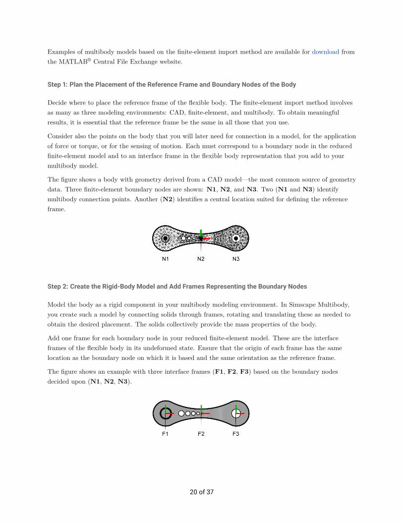
The figure shows a body with geometry derived from a CAD model—the most common source of geometrydata. Three finite-element boundary nodes are shown: N1, N2, and N3. Two (N1 and N3) identifymultibody connection points. Another (N2) identifies a central location suited for defining the referenceframe.

Step 2: Create the Rigid-Body Model and Add Frames Representing the Boundary Nodes

Model the body as a rigid component in your multibody modeling environment. In Simscape Multibody,you create such a model by connecting solids through frames, rotating and translating these as needed toobtain the desired placement. The solids collectively provide the mass properties of the body.

Add one frame for each boundary node in your reduced finite-element model. These are the interfaceframes of the flexible body in its undeformed state. Ensure that the origin of each frame has the samelocation as the boundary node on which it is based and the same orientation as the reference frame.

The figure shows an example with three interface frames (F1, F2, F3) based on the boundary nodesdecided upon (N1, N2, N3).

20 of 37

Step 3: Place Deflection Joints Between the Rigid-Body Model and the Interface Frames

Attach a joint to each interface frame with the exception of one. The joints are those described in section3.1.3—the deflection joints. They capture the displacements of the interface frames of the flexible bodyrelative to those defined in step 2, their counterparts in the undeformed state. Configure each deflectionjoint for connection to the state-space representation that you later create. Select:

• Position, velocity, and acceleration as the joint sensing outputs

• Force and torque as the joint actuation inputs

The degrees of freedom of the deflection joints determine the types of deformation that the body is capableof. Use joints with six degrees of freedom to capture all possible types of deformation. The interface frameleft without a deflection joint serves as the zero-deflection reference in your model. The deflections of allother interface frames are defined against this reference. For more information, see sections 3.1.4 and 3.4.2.

Step 4: Create the Deformation Model and Connect It to the Deflection Joints

Formulate the state-space system introduced in section 3.1.1:

Ûx = Ax + Bu and y = Cx + Du. (20)

Determine the state-space matrices (A, B, C, and D) in terms of the mass, stiffness, and damping matricesof your reduced finite-element model. The matrix calculations are detailed in section 3.4.4.

The state-space system is your deformation model. In Simulink®, you can represent a state-space systemusing the State-Space block. Use the motion sensing outputs from the deflection joints as the inputs toyour state-space system. Use the force and torque outputs from the state-space system as the inputs toyour deflection joints.

21 of 37

Step 5: Extract the Reduced Mass and Stiffness Matrices from the Finite-Element Model

Configure the finite-element model of the flexible body using your preferred finite-element application.Ensure that the reference frame matches the frame previously established for the rigid body anddeformation models. Ensure also that the boundary nodes in your finite-element model correspond to theinterface frames in the rigid-body model.

Finally, configure the number of vibration modes to retain and generate the reduced finite-element model.Extract the mass, stiffness, and, if provided, damping matrices and add them as parameters to thestate-space representation of the deformation model. These matrices are used in the calculation of thevarious state-space matrices.

3.3 Guidelines

3.3.1 Algebraic Loops

As noted in section 3.1.3, deflection joints each connect to the deformation model via a feedback loop. If afeedback loop is such that the output of a calculation at a time step depends on its own value at that timestep, that feedback loop is also an algebraic loop. Algebraic loops can be difficult to solve and often slowdown simulation.

In Simulink terms, an algebraic loop is one that consists entirely of direct-feedthrough blocks—those whoseoutputs at a time step depend directly on their inputs at that time step. You can break a Simulinkalgebraic loop by adding to it a block that does not behave as direct-feedthrough.

A suitable option in a Simscape Multibody model is the Simulink Transfer Fcn block. Simply insert theblock in the algebraic loop and use its parameters to specify the first-order transfer function

1τs + 1

, (21)

where τ is a characteristic time constant—a measure of the time taken by the output signal to reach 63%of its steady-state value when given a step input signal.

22 of 37

The addition of a transfer function to an algebraic loop introduces in that loop a slight time delay. Thedelay is proportional to the characteristic time constant and it can, in certain cases, significantly impactthe transient response of the model. You can mitigate such an impact by specifying a sufficiently smalltime constant.

For the most accurate results, the time constant should be no greater than half the period of the fastestoscillation mode in your model. Start with a value an order of magnitude smaller and fine-tune it ifnecessary. Avoid values that are much smaller as these can negatively impact the speed of simulation.

3.3.2 Interface Inertias

The interface frames of a flexible body connect internally to deflection joints and externally to multibodyjoints, those placed not within but between bodies. Because the interface frames have no inertia of theirown, you must rigidly connect to each a component that does. Every joint should connect on each side toan inertia and this step helps to fulfill this requirement. You can conceive of the interface inertias indifferent ways:

a) As modeling artifacts introduced to prevent simulation errors and to ensure a reasonable simulationspeed. The interface inertias are negligible and do not correspond to a physical part of the flexible body.The inertial properties should be neither so large as to impact model dynamics nor so small as to allowsimulation errors to occur.

b) As small sections of the flexible body, such as the tips, or ends, at which a mechanical link connects toother bodies. The interface inertias are small and correspond to a physical portion of the body.

c) As sizeable sections of the flexible body, split from the rigid-body model to more precisely reflect thedistribution of inertia during deformation. The interface inertias are substantial and correspond to aphysical part of the body.

Option c produces the most accurate simulation results. The reason is two-fold. Partly, the mass propertiesof a flexible body change as it deforms. These are, however, specified as constants in the rigid-body model

23 of 37

and a discrepancy therefore arises between simulation and the physical world. Splitting the mass propertiesover the interface frames allows you to more closely capture their distribution during deformation.

Note also that the rigid-body model is fixed only to the reference frame. An external force applied therehas to overcome the full inertia of the body. The same is not true of an external force applied at a differentinterface frame. Splitting the mass properties over the interface frames allows you to more evenlydistribute their effects and correct for this issue.

3.3.3 Body Visualization

One interface frame must serve as reference for the measurement of deflection. The reference frame ischosen to be coincident with an interface frame and its deflection is therefore always zero. This conventionis enforced by removing from the frame all of its deflection degrees of freedom—that is, by ensuring thatthe interface frame connects to the rigid-body model not through a deflection joint but through a rigidconnection.

Your selection of reference frame impacts your visualization results. Figure 19 shows an example: a binarylink with three interface frames, two at its ends and one at its center. The reference frame is at theleftmost end in case I, at the center in case II, and at the rightmost end in case III. The shaded areasdepict the geometry of the body in the undeformed configuration. They correspond to the rigid-bodymodel. The curved lines depict the interface frames in a deformed configuration. They correspond to thedeformation model.

Figure 19: Flexible body visualization with reference frame at different locations

Note that the interface frames (through which the body connects to its neighbors) lie on the curved linescorresponding to the deformation model. Deformation is shown as identical in all three cases. Theplacement of the rigid-body model varies significantly from case to case and causes deformation to appearto differ. In addition, because the displacements of the deflection joints are measured against differentreference frames, these too may differ. Splitting the inertia of the body into sizeable portions and assigninga geometry to each generally improves the visualization results.

3.4 Theory

The constituents of a flexible-body model and the relationships between them are represented in aSimscape Multibody model by means of blocks and connection lines. The most noteworthy of these isperhaps the Simulink State-Space block that in the examples of section 3.5 comprises the deformationmodel. The challenge of the finite-element import method reduces largely, in this case, to the calculation ofthe State-Space block parameters. These include the A, B, C, and D matrices of the state-space system

24 of 37

given by equations (18) and (19). This section describes how you can reduce a finite-element model and,from its mass, stiffness, and damping matrices, obtain the required state-space matrices.

3.4.1 Model Reduction

Recall from the discussion of section 3.1.1 that the state-space matrices derive from a reduced form of afinite-element model. This paper focuses on a model reduction method first presented in 1968 by R. Craigand M. Bampton3 . This method has since found widespread application in the analysis of multibodyproblems. Its use of boundary nodes, and the direct mapping of these to interface frames, makes itespecially convenient for the finite-element import method.

A model reduction method serves to reduce the complexity (and therefore size) of a model. TheCraig-Bampton method achieves this reduction by eliminating all fixed-boundary vibration modes whosefrequencies are above a certain cutoff. The result is a simplified model, with fewer variables, and withsmaller mass and stiffness matrices. You can, by carefully selecting the cutoff frequency, preserve theessential dynamic characteristics of the model.

The Craig-Bampton method generally proceeds as follows:

1. Split the nodes of a finite-element mesh into internal and boundary sets.

2. Express the degrees of freedom of the partitioned nodes in terms of boundary and modalcoordinates.

3. Truncate the set of modal coordinates at a designated cutoff frequency.

4. Reformulate the model in terms of the reduced degrees of freedom—the physical coordinates of theboundary nodes and the truncated modal coordinates.

From the discussion of section 3.1.1, the undamped nodal motions in a finite-element mesh can beexpressed as

M Üud +Kud = f . (22)

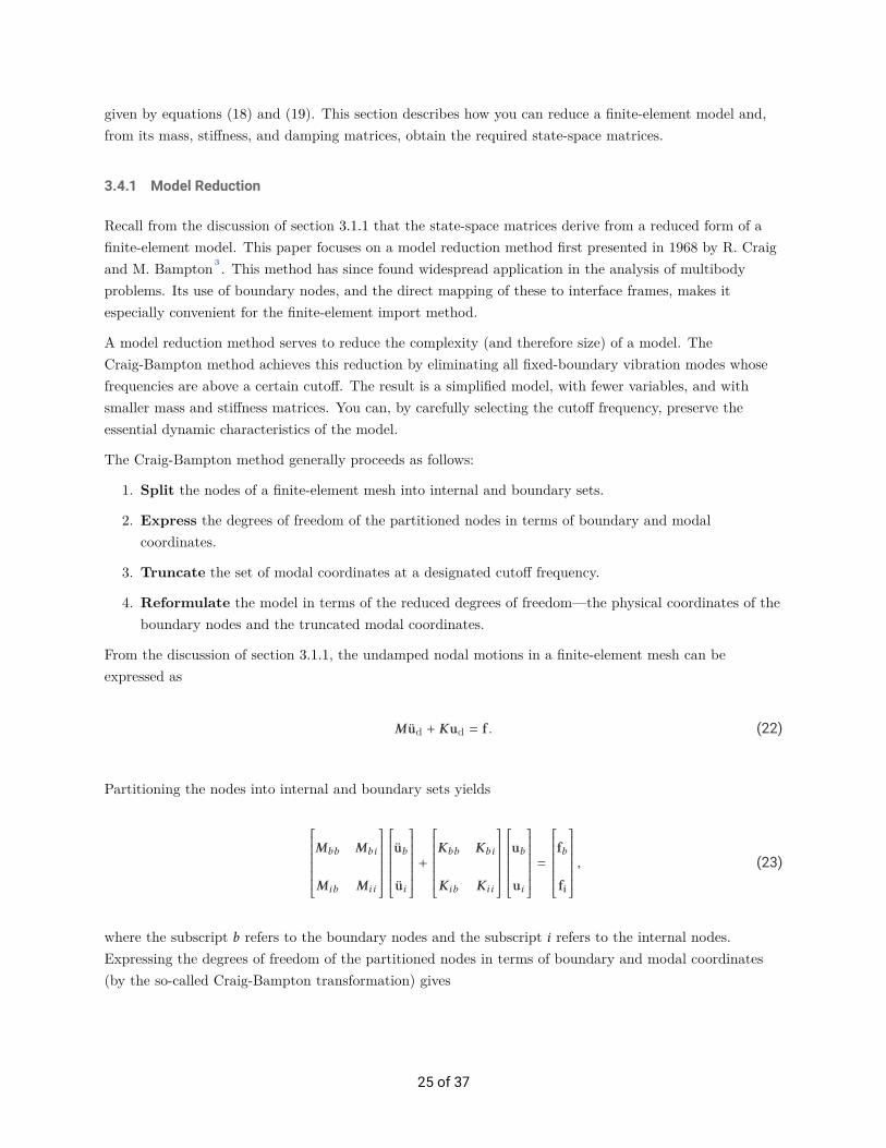
Partitioning the nodes into internal and boundary sets yields

Mbb Mbi

Mib Mii

Üub

Üui

+Kbb Kbi

Kib Kii

ub

ui

=fb

fi

, (23)

where the subscript b refers to the boundary nodes and the subscript i refers to the internal nodes.Expressing the degrees of freedom of the partitioned nodes in terms of boundary and modal coordinates(by the so-called Craig-Bampton transformation) gives

25 of 37

ub

ui

= H

ub

η

, (24)

where η is the set of modal degrees of freedom—the modal amplitudes resulting from the assumption thatthe boundary nodes are fixed. The degrees of freedom in [ub η] form a hybrid set, with some (ub) definedin physical space and some (η) defined in modal space. H is the Craig-Bampton transformation matrix,

H =

[Ξ Φ

], (25)

where Ξ is a set of constraint, or static condensation, modes, and Φ is a set of fixed-boundary mode shapes.Truncating the modal coordinates at a cutoff frequency—thereby discarding the lowest-amplitude modes,which lie above the cutoff—gives

ub

ui

' H

ub

η∗

, (26)

where η∗ is the set of truncated, or reduced, modal degrees of freedom. Rewriting the equation of motion interms of the reduced degrees of freedom gives the final working expression

M̂bb M̂bm

M̂mb M̂mm

Üub

Üη∗

+K̂bb K̂bm

K̂mb K̂mm

ub

η∗

=fb

0

, (27)

where the M̂∗∗ terms comprise the reduced mass matrix M̂ and the K̂∗∗ terms comprise the reduced stiffnessmatrix K̂ :

M̂ = HTMH and K̂ = HTKH . (28)

Subscript m refers to the vibration modes of the body. External forces are assumed to act exclusively atthe boundary nodes (that is, fi = 0). This result is the Craig-Bampton equation of motion and the reducedmatrices in it are, with additional processing, the basis for the calculation of the state-space matrices. Thereduced matrices are often provided by finite-element modeling software.

26 of 37

3.4.2 Rigid-Body Modes

The Craig-Bampton model captures not only the vibration modes of the flexible body but also therigid-body modes—the translations and rotations of the body in the absence of deformation. Recall fromsection 3.1 that in the finite-element import method rigid-body motion is captured via the rigid-bodymodel alone. You must therefore ensure that the deformation model, and the Craig-Bampton model uponwhich it is based, is free of rigid-body modes.

There are, in the general case, six rigid-body modes. A body in 3-D space can at a maximum translate inthree perpendicular directions and rotate in three perpendicular planes. If the boundary nodes of theCraig-Bampton model have six degrees of freedom each, then the rigid-body modes can be removed byfixing one boundary node and setting all of its deflections to zero.

Consider again the Craig-Bampton equation of motion. Expanding the matrix terms to more explicitlyshow the degrees of freedom of the boundary nodes yields

M̂11 · · · M̂1n M̂1m

.... . .

......

M̂n1 · · · M̂nn M̂nm

M̂m1 · · · M̂mn M̂mm

Üu1

...

Üun

Üη∗

+

K̂11 · · · K̂1n K̂1m

.... . .

......

K̂n1 · · · K̂nn K̂nm

K̂m1 · · · K̂mn K̂mm

u1

...

un

η∗

=

f1

...

fn

0

, (29)

where subscripts 1 through n refer to the boundary nodes and each node is assumed to have six degrees offreedom. Suppose that you elect to fix boundary node 1 and set all of its possible deflections, threetranslational and three rotational, to zero. The Craig-Bampton equation, minus the duplicate degrees offreedom, becomes

M̂22 · · · M̂2n M̂2m

.... . .

......

M̂n2 · · · M̂nn M̂nm

M̂m2 · · · M̂mn M̂mm

Üu2

...

Üun

Üη∗

+

K̂22 · · · K̂2n K̂2m

.... . .

......

K̂n2 · · · K̂nn K̂nm

K̂m2 · · · K̂mn K̂mm

u2

...

un

η∗

=

f2

...

fn

0

. (30)

The first row and column of each matrix has been removed. Had boundary node 2 been fixed instead, thesecond row and column would have been removed. Note that if your choice of fixed boundary node changes,your choice of reference interface frame must too. See section 3.1.4 for more on the reference frame.

The state-space system comprising the deformation model is calculated in part from the matrices ofequation (30). The calculations are discussed in greater detail in section 3.4.4.

27 of 37

3.4.3 Modal Damping

A true flexible body does not, in the absence of a driving force, vibrate forever. It loses energy with eachcycle due to damping. The mechanisms of damping are varied and often difficult to characterize, but youcan approximate their effects using a simple linear model. Adding to the reduced equation of motion alinear damping term L̂ yields the expression:

M̂bb M̂bm

M̂mb M̂mm

Üub

Üη∗

+L̂bb L̂bm

L̂mb L̂mm

Ûub

Ûη∗

+K̂bb K̂bm

K̂mb K̂mm

ub

η∗

=fb

0

, (31)

where L̂∗∗ are submatrices of L̂. Some modeling applications may provide the reduced damping matrix for areduced finite-element model. Alternatively, you can obtain the damping matrix by direct calculation,using as a basis an appropriate model of damping. For a discussion of common damping models and of thematrix calculations that they entail, see Fundamentals of Structural Dynamics, by R. Craig and A.Kurdila4.

A damping model in widespread use is that known as modal damping. This model assumes that thedamping matrix can be diagonalized by a modal transformation. The values of the diagonal matrixelements are each calculated from a modal damping factor (ζi ). The overall calculation can be summarizedas follows:

1. Perform a modal analysis of the reduced finite-element model and obtain its normal mode shapes (Ψ)and natural frequencies.

2. Transform the Craig-Bampton equation of motion—equation (31)—into modal coordinate space andadd a modal damping term L̄ Ûq:

M̄ Üq + L̄ Ûq + K̄q = f̄ , (32)

where q are the modal degrees of freedom. The term f̄ =ΨTf̂ is the modal force vector and the termsM̄, L̄, and K̄ are the modal mass, damping, and stiffness matrices. These matrices are related to theirCraig-Bampton counterparts (M̂, L̂, and K̂) by the expressions

M̄ =ΨTM̂Ψ , L̄ =ΨTL̂Ψ , K̄ =ΨTK̂Ψ . (33)

3. Construct the modal damping matrix. As mentioned previously, and akin to the mass and stiffnessmatrices, the damping matrix is assumed to be diagonalized by a modal transformation. Calculate thediagonal matrix elements by assuming them each to be a viscous damping term of the form 2ωiζiMi :

28 of 37

L̄ =

2ω1ζ1M1

. . .

2ωNζNMN

, (34)

where ωi are the natural frequencies, ζi the modal damping factors, and Mi the elements of the(diagonal) modal mass matrix.

4. Transform the modal damping matrix into the reduced coordinate space employed in theCraig-Bampton equation. The final result is an expression of the form4

L̂ =(M̂ΨM̄−1

)L̄

(M̄−1ΨTM̂

), (35)

where Ψ is the modal matrix of the flexible body.

3.4.4 State-Space System

Consider again the state-space representation of the deformation model (equations (18) and (19) of section3.1.1):

Ûx = Ax + Bu and y = Cx + Du.

In the finite-element import method, the states (x) of this system are defined as the amplitudes, orparticipation factors, of the various vibration modes (η):

x =

η∗

Ûη∗

. (36)

Similarly, the inputs (u) are defined as the deflections of the boundary nodes (ub)—or, equivalently, of theinterface frames, relative to the common reference frame described in section 3.1.4:

u =

ub

Ûub

Üub

. (37)

29 of 37

Finally, the outputs (y) are the internal forces and torques (−fb) that arise naturally in the body as aconsequence of the nodal deflections. These forces and torques are opposite to the external applied loadsthat would produce those deflections:

y = −fb. (38)

Casting the state-space matrices in terms of the reduced mass, damping, and stiffness matrices obtainedfrom the reduced finite-element model gives, for the state matrix,

A =

O I

−M̂−1mmK̂mm −M̂−1

mmL̂mm

; (39)

for the input matrix,

B =

O O O

−M̂−1mmK̂mb −M̂−1

mmL̂mb −M̂−1mmM̂mb

; (40)

for the output matrix,

C =

[−

(K̂bm − M̂bmM̂

−1mmK̂mm

)−

(L̂bm − M̂bmM̂

−1mmL̂mm

)]; (41)

and for the direct-feedthrough matrix,

D =

[−

(K̂bb − M̂bmM̂

−1mmK̂mb

)−

(L̂bb − M̂bmM̂

−1mmL̂mb

)−

(M̂bb − M̂bmM̂

−1mmM̂mb

)]. (42)

3.5 Examples

3.5.1 Flexible Cantilever Beam

Consider the flexible cantilever beam first discussed in section 2.4.1. The properties of the beam are thosedescribed there. The loading conditions are likewise the same—one a distributed gravitational load(associated with a gravitational acceleration 100 times that of Earth), the other a beam subjected to anupward point force of 20 N in a zero-gravity environment.

30 of 37

Model Parameters The beam model considered here contains three interface frames. The inertia of thebeam is split over the interface frames in sizeable chunks—the conceptual case described in item c ofsection 3.3.2. As is encouraged in section 3.1.4, the reference frame of the body is located at the center ofthe beam.

The deformation model is based on a finite-element model reduced by the Craig-Bampton method to thefirst 20 vibration modes. The feedback loops between the deformation model and the deflection joints eachcontain a first-order filter of time constant 1e-7 s. The filter is based on the transfer function described insection 3.3.1.

Modal damping is included in the model in the matrix form described in equation (34). The dampingparameter ζ used to construct the damping matrix is set to a value of 0.05.

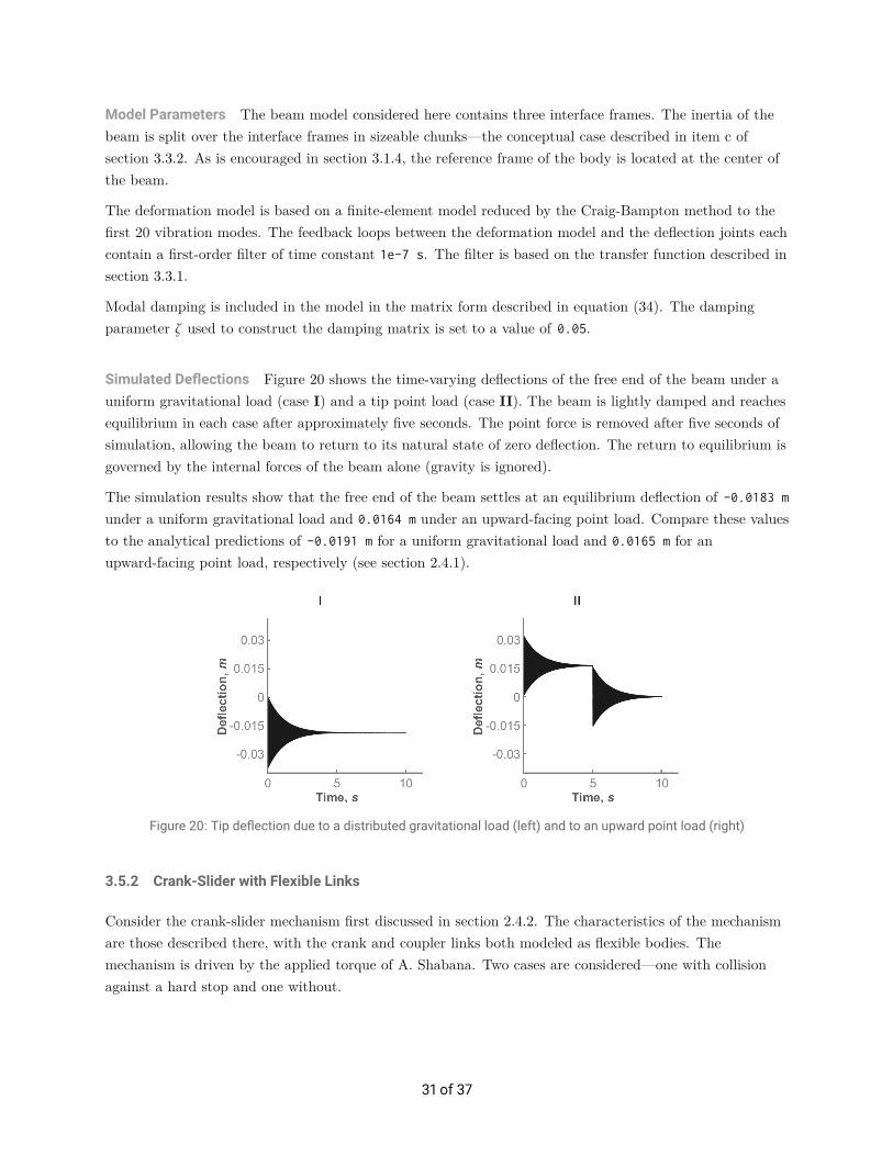
Simulated Deflections Figure 20 shows the time-varying deflections of the free end of the beam under auniform gravitational load (case I) and a tip point load (case II). The beam is lightly damped and reachesequilibrium in each case after approximately five seconds. The point force is removed after five seconds ofsimulation, allowing the beam to return to its natural state of zero deflection. The return to equilibrium isgoverned by the internal forces of the beam alone (gravity is ignored).

The simulation results show that the free end of the beam settles at an equilibrium deflection of -0.0183 m

under a uniform gravitational load and 0.0164 m under an upward-facing point load. Compare these valuesto the analytical predictions of -0.0191 m for a uniform gravitational load and 0.0165 m for anupward-facing point load, respectively (see section 2.4.1).

Figure 20: Tip deflection due to a distributed gravitational load (left) and to an upward point load (right)

3.5.2 Crank-Slider with Flexible Links

Consider the crank-slider mechanism first discussed in section 2.4.2. The characteristics of the mechanismare those described there, with the crank and coupler links both modeled as flexible bodies. Themechanism is driven by the applied torque of A. Shabana. Two cases are considered—one with collisionagainst a hard stop and one without.

31 of 37

Model Parameters The crank and coupler are modeled by the finite-element import method and giventhree interface frames each. The remaining bodies are treated as rigid. The inertias of the flexible bodiesare split over the interface frames in sizeable chunks (item c of section 3.3.2). For improved accuracy, thereference frames are each placed at a central location on the body.

The deformation model is based on a finite-element model reduced by the Craig-Bampton method to thelowest-frequency vibration modes. The feedback loops between the deformation model and the deflectionjoints each contain a first-order filter of time constant 1e-7 s. The filter is based on the transfer functiondescribed in section 3.3.1.

Modal damping is included in the model in the matrix form described in equation (34). The dampingparameter ζ used to construct the damping matrix is set to a value of 0.05.

Simscape Multibody Model Figure 21 shows a Simscape Multibody model of the crank-slider mechanism.The crank, coupler, and slider, connect to each other and to the world by means of joints. The drivingtorque is applied directly to the revolute joint that connects the crank to the world. The hard-stop force isapplied directly to the prismatic joint that connects the slider to the world.

Figure 21: Simscape Multibody model of a crank-slider mechanism

Figure 22 shows the Simscape Multibody representation of one flexible body—the coupler. A Solid block(named Rigid Body) comprises the rigid-body model. A Simulink State Space block (State SpaceSystem) comprises the deformation model. The two models connect through deflection joints, eachenclosed in a Simulink Subsystem block (Deflection Joint 1–2). A third Simulink Subsystem (RigidConnection) denotes the connection to the chosen reference frame.

32 of 37

Figure 22: Simscape Multibody model of a flexible coupler

The interface frames are denoted by Simscape Physical Connection blocks (named B, M, and F). Theinterface inertias are specified through Simulink Subsystem blocks (Inertia F1–F3), each enclosing a Solidblock. The three Rigid Transform blocks (Transform Frame 1–3) merely define the placement of theframes through which the rigid-body model connects to the deflection joints.

Simulated Deflections Figure 23 overlays the simulation results obtained here using the finite-elementimport method (curve B) on those published by A. Shabana (curve A). The curves each correspond to thetransverse deflection measured at the midpoint of the coupler link with respect to an imaginary line drawnbetween the longitudinal ends of the same link.

Figure 23: Comparison to Shabana 2 simulation results (A: Shabana, B: Simscape Multibody)

Figure 24 shows the simulation results obtained from a model with an obstacle—a translational hard

33 of 37

stop—placed in the path of the slider. Contact occurs shortly after the 0.5-second mark, inducing in thecoupler link the vibrations shown. As before, the results correspond to the transverse deflection measuredat the midpoint of the coupler link. The oscillations decay at a rate determined by the damping matrixused in the model.

Figure 24: Coupler deflection due to contact

Simulation Accuracy The simulation results depend closely on the configuration of the model. Thenumber of interface frames, the number of vibration modes, the location of the reference frame (that towhich the rigid-body model is fixed), and the partitioning of inertia among the interface frames can allimpact the dynamics of the flexible body.

Figure 25 shows, in a model without an obstacle, the effect of changing the number of interface frames.Curve A corresponds to a model with three interface frames per flexible body. Curve B corresponds to amodel with five interface frames per flexible body. Increasing the number of interface frames improves theaccuracy of the model. Results by A. Shabana are overlaid in bold. The crank and coupler are eachmodeled with a centrally located reference frame and equitably partitioned interface inertias.

Figure 25: Effect of changing the number of interface frames (A: three interface frames, B: five interface frames)

Figure 26 shows the effect of partitioning the inertia over the various interface frames. Curve A correspondsto a model in which the interface inertias are negligible. Curve B corresponds to a model in which inertiahas been more equitably distributed over the interface frames. Partitioning the inertia equitably over the

34 of 37

interface frames improves the accuracy of the model. Results by A. Shabana are overlaid in bold. Thecrank and coupler are each modeled with three interface frames and a centrally located reference frame.

Figure 26: Effect of partitioning the inertia over the interface frames (A: negligible interface inertias, B: sizeable interfaceinertias)

The selection of reference frame can have an especially significant impact on your simulation results.Figure 27 shows the effect of switching the reference frames of the flexible bodies each from an interfaceframe at an end (curve A) to one near the center (curve B). Placing the reference frame at a centrallocation improves the accuracy of the model. Results by A. Shabana are overlaid in bold. The crank andcoupler are each modeled with three interface frames and equitably partitioned interface inertias.

Figure 27: Effect of changing the placement of the reference frame (A: reference frame near tip, B: reference frame nearcenter)

Visualization Results Figure 28 shows the visualization results obtained from a Simscape Multibodymodel of the crank-slider mechanism. The coupler is modeled as a rigid body in case I, as a flexible bodywith three interface frames in case II, and as a flexible body with five interface frames in case III. Inertia issplit over the interface frames in cases II and III. In each case, the model is shown as it appears an instant(0.05 s) after collision with the hard stop.

35 of 37

Figure 28: Visualization with the coupler as a rigid body (I) and as a flexible body with three (II) and five (III) interfaceframes

Deformation is made evident in this figure in two ways. First, the interface inertias are modeled as solidswith geometry, each a section of the coupler beam. These geometries comprise the entirety of the couplerin the visualization results. Second, spherical markers are appended to the interface frames, making thedeflections of those frames more evident.

The coupler is naturally undeformed in case I. It is slightly deformed in case II but, due to the smallnumber of interface frame solids, its visualization has a staggered appearance. The same deformation isevident in case III, now with smoother visualization results produced by the greater number of interfaceframe solids used.

4 Conclusion

You can represent a flexible body in a multibody model using lumped-parameter and finite-element importmethods. The lumped-parameter method discretizes the body into flexible units, each comprising two masselements coupled through a joint with an internal spring and an internal damper. This method provides asimple solution for bodies with slender geometries, with an accuracy that depends largely on the number offlexible units used.

The finite-element import method splits the flexible body into a rigid-body model and a deformation modeland superposes their respective motions. The deformation model is implemented as a state-space systemcreated from data that you obtain from a reduced finite-element model. This method provides a superiorsolution for general 3-D geometries, with an accuracy that depends on the number of interface frames, thepartitioning of mass properties, the location of the reference frame, and the number of vibration modes.

The examples show that the lumped-parameter method improves in accuracy when the number of flexibleunits increases in number—though above a certain discretization level any subsequent increases in accuracybecome negligible. Similarly, the finite-element import method improves in accuracy when the interfaceframes increase in number, when the inertia of the body is more equitably split over the interface frames,and when the reference frame is centrally located on the body.

36 of 37

References

[1] Simscape Multibody Documentation . MathWorks.

[2] Shabana, Ahmed A. Dynamics of Multibody Systems . 4th ed. Cambridge University Press, 2013.

[3] Craig, Roy R. and Bampton, Mervyn C. Coupling of Substructures for Dynamic Analyses . AIAAJournal 6, no. 7 (1968): 1313–1319.

[4] Craig, Roy R. and Kurdila, Andrew J. Fundamentals of Structural Dynamics . 2nd ed. John Wiley &Sons, 2006.

[5] Miller, S. Flexible Body Models in Simscape Multibody . MathWorks.

W H I T E PA P E R | 3 7

© 2017 The MathWorks, Inc. MATLAB and Simulink are registered trademarks of The MathWorks, Inc. See mathworks.com/trademarks for a list of additional trademarks. Other product or brand names may be trademarks or registered trademarks of their respective holders.

TECHNICAL PAPER