modeling economic output and economic growth …838543/fulltext01.pdfmodeling economic output and...
TRANSCRIPT

DEGREE PROJECT, IN APPLIED MATHEMATICS AND INDUSTRIAL, FIRST LEVELECONOMICS
STOCKHOLM, SWEDEN 2015
Modeling Economic Output andEconomic Growth with respect toEconomic Freedom
A COMPARATIVE STUDY OF DEVELOPINGAND DEVELOPED COUNTRIES
ERIK JOHANSSON, ERIK TRETOW
KTH ROYAL INSTITUTE OF TECHNOLOGY
SCI SCHOOL OF ENGINEERING SCIENCES


Modeling Economic Output and Economic Growth with respect to Economic Freedom:
A comparative study of developing and developed countries
E R I K J O H A N S S O N E R I K T R E T O W
Degree Project in Applied Mathematics and Industrial Economics (15 credits)
Degree Progr. in Industrial Engineering and Management (300 credits) Royal Institute of Technology year 2015
Supervisors at KTH: Boualem Djehiche, Anna Jerbrant Examiner: Boualem Djehiche
TRITA-MAT-K 2015:10 ISRN-KTH/MAT/K--15/10--SE Royal Institute of Technology School of Engineering Sciences KTH SCI SE-100 44 Stockholm, Sweden URL: www.kth.se/sci

2
Abstract
This Bachelor thesis is an empirical comparative study examining the relationship
between economic performance and economic freedom in two sample groups consisting
of 25 developed and 25 developing countries respectively. The relationship is analyzed
with results from ordinary and robust linear regressions using an extended Solow-Swan
exogenous growth model. The obtained results show a significant positive correlation
between economic freedom and economic output (GDP/capita), while the correlation is
shown to be insignificant for economic growth.
Acknowledgements
We thank
Boualem Djehiche, our supervising professor in mathematical statistics - for your guidance
and sharing your great insights in mathematics.
Anna Jerbrant, from the department of Industrial Engineering and Management - for your
guidance, feedback and encouragement.
Oskar Broström and Marcus Larsson - for your moral support and company during late
night study sessions.


3
Table of contents
Abstract .................................................................................................................................................... 2
Acknowledgements ............................................................................................................................. 2
Table of contents .................................................................................................................................. 3
1 Introduction ................................................................................................................................. 7
1.1 Background to thesis ....................................................................................................................... 7
1.2 Problem statement ........................................................................................................................... 8
1.3 Scope ....................................................................................................................................................... 8
1.4 Previous research on economic freedom and economic growth ................................. 8
1.5 Relevance .............................................................................................................................................. 9
1.6 Qualitative method ........................................................................................................................... 9
1.6.1 Design ................................................................................................................................................ 9
1.6.2 Search strategy and literature research ............................................................................ 9
2 Macroeconomics of economic performance ................................................................... 12
2.1 Definitions ......................................................................................................................................... 12
2.1.1 GDP .................................................................................................................................................. 12
2.1.2 Economic output ....................................................................................................................... 12
2.1.2 Economic growth ...................................................................................................................... 12
2.1.2 Developing and developed countries ............................................................................... 13
2.1.3 Economic freedom .................................................................................................................... 13
2.1.4 Human capital ............................................................................................................................. 13
2.1.5 Social infrastructure ................................................................................................................ 13
2.2 Theory on economic growth ..................................................................................................... 13
2.2.1 The Solow-Swan model .......................................................................................................... 13
2.2.2 Convergence according to the Solow-Swan growth model .................................... 16
2.2.3 Extending the Solow-Swan model ..................................................................................... 16
2.3 Composing the linear regression model .............................................................................. 17
2.3.1 Assumptions ................................................................................................................................ 17
2.3.2 Identifying the key drivers of economic output and growth ................................. 17
2.3.3 GDP growth rate or GDP level? ........................................................................................... 18
3 Regression analysis ................................................................................................................. 19
3.1 Linear regression ............................................................................................................................ 19
3.2 Ordinary least squares (OLS) .................................................................................................... 20

4
3.3 Assumptions ..................................................................................................................................... 21
3.3.1 Homoskedasticity ..................................................................................................................... 21
3.3.2 Linear independence ............................................................................................................... 21
3.3.3 Exogeneity .................................................................................................................................... 22
3.4 Transgressions of assumptions................................................................................................ 22
3.4.1 Heteroskedasticity .................................................................................................................... 22
3.4.2 Multicollinearity ........................................................................................................................ 22
3.4.3 Endogeneity ................................................................................................................................. 23
3.7 Hypothesis testing (F-test)......................................................................................................... 24
3.8 Transformation of variables ...................................................................................................... 25
3.8.1 Exponential transformation ................................................................................................. 25
3.9 Coefficient of determination (𝑅2) ........................................................................................... 25
3.10 Akaike information criterion (AIC) ........................................................................................ 26
3.11 Variance inflation factor (VIF) .................................................................................................. 27
3.12 Breusch-Pagan test ........................................................................................................................ 27
3.13 Robust regression models .......................................................................................................... 27
4 Quantitative methodology .................................................................................................... 29
4.1 Response variable .......................................................................................................................... 29
4.2 Covariates .......................................................................................................................................... 29
4.2.1 Covariate scaling ....................................................................................................................... 30
4.3 Data ....................................................................................................................................................... 30
4.3.1 Adjustments on data ................................................................................................................ 31
4.3.2 Source criticism ......................................................................................................................... 31
4.4 Initial regression models ............................................................................................................ 32
4.4.1 GDP/capita level regression model .................................................................................. 32
4.4.2 GDP/capita growth regression model ............................................................................. 32
4.4.3 Expected outcome of coefficient estimates ................................................................... 33
4.5 Algorithm for model improvement ........................................................................................ 34
5 Results for economic output ................................................................................................. 36
5.1 Initial regression for economic output in developing countries ............................... 36
5.2.1 Variance inflation-test for multicollinearity ................................................................. 36
5.2.2 Breusch-Pagan test for heteroskedasticity .................................................................... 36
5.2.3 Distribution of residuals ........................................................................................................ 37

5
5.3 Initial regression for economic output in developed countries ................................ 37
5.3.1 Variance inflation-test for multicollinearity ................................................................. 38
5.3.2 Breusch-Pagan test for heteroskedasticity .................................................................... 38
5.3.3 Distribution of residuals ........................................................................................................ 39
5.4 AIC analysis of the initial OLS regressions .......................................................................... 39
5.4.1 Developing countries .............................................................................................................. 39
5.4.2 Developed countries ................................................................................................................ 40
5.5 Final model ........................................................................................................................................ 40
5.5.1 Developing countries .............................................................................................................. 40
5.5.2 Developed countries ................................................................................................................ 41
5.6 Economic output and economic freedom ............................................................................ 41
5.6.1 Developing countries .............................................................................................................. 42
5.6.2 Developed countries ................................................................................................................ 42
6 Results for economic growth ................................................................................................ 43
6.1 Diagnosing for multicollinearity .............................................................................................. 43
6.1.1 Initial OLS for developing countries ................................................................................. 43
6.1.2 Initial OLS for developed countries .................................................................................. 43
6.2 Presence of heteroskedasticity ................................................................................................ 44
6.2.1 Initial OLS for developing countries ................................................................................. 44
6.2.2 Initial OLS for developed countries .................................................................................. 45
6.3 Initial robust regression .............................................................................................................. 46
6.3.1 Developing countries .............................................................................................................. 46
6.3.2 Developed countries ................................................................................................................ 46
6.4 Final robust regression ................................................................................................................ 47
6.4.1 Developing countries .............................................................................................................. 47
6.4.2 Developed countries ................................................................................................................ 48
6.5 Economic freedom and economic growth rate ................................................................. 49
6.5.1 Developing countries .............................................................................................................. 49
6.5.2 Developed countries ................................................................................................................ 49
6.6 The convergence hypothesis of the non-extended Solow-Swan model ................. 50
7 Discussion ................................................................................................................................... 51
7.1 Result analysis – evaluation of the estimated coefficients ........................................... 51
7.1.1 Accounting for endogeneity – are the results reliable?............................................ 51
6
7.1.2 Economic output ....................................................................................................................... 52
7.1.3 Economic growth ...................................................................................................................... 55
7.2 What are the effects on GDP/capita level and GDP/capita growth from economic
freedom among developing and developed countries? ................................................................. 57
7.4 Concluding remarks ...................................................................................................................... 58
7.5 Suggestions for further research ............................................................................................. 58
8 References ................................................................................................................................... 60
8.1 Data sources ..................................................................................................................................... 62
8.1.1 Data used in regression .......................................................................................................... 62
8.1.2 Miscellaneous ............................................................................................................................. 62
A Appendix ...................................................................................................................................... 63
A1 Samples of developing and developed countries ............................................................. 63
A2 Motivations for initial expectations of coefficient estimate outcomes ................... 64

7
1 Introduction
1.1 Background to thesis
The governing dynamics behind the output of an economy (GDP) is subject to constant
debate in economics. What makes an economy prosper and why are some countries more
prosperous than others? Alongside the debate, extensive theoretical and empirical
research has tried to answer this question.
The original neoclassical growth model from economists Solow (1956) and Swan (1956)
suggest that the GDP of poor countries will - under the right conditions - grow faster than
the GDP of rich countries, which is why the starting level of income must be of importance
to economic growth. The models did not provide a satisfying explanation for why
productivity was lower in poorer countries, but it laid the foundation for empirical
research on the subject.
Extensions from economists Romer et al. (1992) provided a model that took human
capital in account for explaining why productivity was lower in developing countries.
Further extensions from Hall & Jones (1999) suggested that social infrastructure also
should be included in the model in order to describe the environment in which agents
ultimately produce economic output. Within the term social infrastructure there are
defining measures such as rule of law, property rights and freedom of contract – all
measures of economic freedom.
The relationship between economic freedom and economic growth has been examined by
researchers with varying results. Notably, De Haan & Sturm (2000), used cross-sectional
data from 80 countries over years 1975-1990 and found that there was a significant
positive correlation between economic growth and changes in economic freedom – but
not between economic growth and the level of economic freedom. Other researchers such
as Scully (2002) and Dawson (2002) found a significant positive correlation between the
level of economic freedom and economic growth.
As mentioned above, most papers have examined the relationship between GDP/capita
growth and economic freedom on a cross-country sample, which arguably signifies short-
term growth (Hall & Jones, 1995). This paper aims to further expand the knowledge on
long-term economic growth by examining the GDP/capita level of 50 countries (of which
25 are developing and 25 developed) in relation to their respective level of economic
freedom, using more recent data from year 2000 to 2013 – as well as the short-term
growth by studying the GDP/capita growth rate. Furthermore, this paper will examine
what impact economic freedom has within the sample groups of developed and
developing countries.

8
1.2 Problem statement
The following research question will be examined, both in context of statistics and
economics:
What are the effects on GDP/capita level and GDP/capita growth from economic freedom
among developing and developed countries?
1.3 Scope
The two individual panels are separated according to the IMF classifications of developing
and developed countries as of 2014. Each panel consists of 25 either developed or
developing countries with an emphasis on geographical and economic diversity within the
classification. Data are from years 2000 to 2013.
1.4 Previous research on economic freedom and economic
growth
Empirical research on the relation between economic freedom and economic performance
(output and growth) is a relatively new area within econometrics. The most cited reports
in this area have in general performed regression analysis on economic growth (not
output) and economic freedom using varying indices of economic freedom. All reports
that have been found use data from periods prior to the year 2000. The following are
some of the most notable research results:
James D. Gwartney, Robert A. Lawson and Randall G. Holcombe (1999) uses an
independently designed index of economic freedom and finds a significant
positive correlation between economic growth and their freedom index on a
cross-section of countries.
Jakob de Haan and Jan-Egbert Sturm (2000) compare different indices for
economic freedom and conclude that they rank countries similarly.
Furthermore, de Haan and Sturm conclude that the level of economic freedom is
not related to economic growth, but that changes in economic freedom are
positively related to economic growth on a cross-section of countries.
Torstensson (1994) finds that the degree of state ownership has no correlation
with economic growth for a cross-section sample group consisting of 68
countries. This study has been criticized by De Haan and Sturm (2000) for
having a limited measure of economic freedom.
Jac C. Heckelman (2000) investigates the causal link between economic freedom
and economic growth and concludes that economic freedom precedes economic

9
growth in all but one (Government Intervention) of the underlying components
of Heritage Foundation’s Index of Economic Freedom.
1.5 Relevance
While the relationship between economic freedom and economic growth has been subject
to research before, most of the research has examined cross-section sample groups with
data from periods prior to year 2000. We believe that there exists differences in the way
one should model economic growth and output when examining developing countries and
developed countries respectively. Furthermore, we expect that the recent financial crisis
in 2008 have played a major part in the economic growth of most economies and that data
from 2000-2013 is interesting in this aspect. Lastly, this thesis examines economic
performance both in terms of economic output (GDP/capita) and economic growth
(GDP/capita growth rate).
1.6 Qualitative method
1.6.1 Design
The following two chapters are based on a basic literature study where the aim is to
inform the reader on the necessary theoretical background used in the regression
analysis. The following questions are researched for the literature study:
1. How is economic output and growth typically modeled?
2. How can a measure of economic freedom be incorporated in these models?
3. How can these models be used in regression analysis?
4. What mathematical tools are necessary for the regression analysis?
The articles and literature subject to research are based on both qualitative and
quantitative studies. The primary source of information is scientific papers, secondarily
educational literature.
1.6.2 Search strategy and literature research
Scientific articles
The search tool that is used throughout the literature study for scientific reports is Google
Scholar. Databases include KTHB Primo and the National Bureau of Economic Research
(NBER) among others.
For chapter 2 and 3, the following search phrases are used in Google Scholar; either alone
or in combinations, with or without the Boolean expression AND:
10
Economic Output, Economic Growth, Economic Freedom, Model, Developing Countries,
Convergence, Human Capital, Regression Analysis, OLS.
For the discussion in chapter 7, Google Scholar is used with the following additional
search phrases; either alone or in combinations, with or without the Boolean expression
AND:
Population growth, financial crisis, life expectancy, GDI, FDI, Great depression.
Educational literature
The educational literature that is being used is either from the course Applied
Mathematical Statistics’ (Course code: SF2950 at KTH) recommended literature or using
the following search words in Google Scholar:
Linear regression, robust regression, VIF, Breusch Pagan, multicollinearity,
heteroskedasticity, scaling covariates, log transformation, economic growth.
Literature selection
The articles and literature were chosen based on the following criteria:
- Is the paper/article relevant to the research question?
- How many times has the article/literature been cited in other research?
- Is the publishing journal credible?
Source criticism
Macroeconomic theories, including the Solow framework used in this thesis, are subject to
constant discussion; there is no single theory on economic output and growth which all
economists agree upon. With this in mind, from our literature study we have found that
the Solow-Swan theory, with its extensions, is the most commonly used in the context of
regression analysis on GDP.
Research by the following authors have formed the foundation of knowledge upon which
the regression models are composed and analyzed: Barro, accompanied by Lee and Sala-i-
Martin (1991, 1994, 1995, 2013), Hall & Jones (1996, 1998) and Mankiw, Romer & Weil
(1992). All of these authors work at respected universities, such as Princeton, MIT and
Harvard, and their work is well cited, with for example the Mankiw-Romer-Weil extension
of the Solow framework having been cited over 12700 times as of May 27, 2015 (NBER).
In chapter 7, where the results are discussed, we look towards more specific research on
the single pairwise relationships between a certain covariate and economic output or
growth. This is done in order to find explanations for when the results do not align with

11
expectations based on initially studied theory. De Haan & Sturm (1999, 2009), with their
articles on the relationship between economic freedom and economic growth, Acemoglu
& Johnsson’s research on the effects of increased life expectancy (2006), as well studies on
financial crises Crotty (2009) and Buiter (2007) make important contributions to this
discussion. When selecting literature references the aim is to reflect different views on
economic freedom and economic growth, in order to avoid ideological bias in the
discussion. We therefore study articles by researchers promoting economic freedom as
well as those wanting to restrict it to some extent.
The reliance of the sources of data used in regressions are discussed in chapter 4 and 7.

12
2 Macroeconomics of economic performance
2.1 Definitions
2.1.1 GDP
The Gross Domestic Product (GDP) is a key measure in economics and is used to quantify
the economic activity within a country or region, commonly on an annual basis. The GDP
can be determined with three different approaches, all of which in theory give the same
results:
Production approach
GDP equals the sum all value added by domestic producers.
Income Approach
GDP equals the sums of factor incomes to the factors of production (land labor, capital,
etc.).
Expenditure Approach
Assuming a free market in perfect equilibrium all produced goods and services are also
purchased, meaning the sum of expenditures must be equal to the added value in
production, thus equal to GDP.
The GDP per capita is the total GDP divided by the population in the country. In general, a
high GDP per capita indicates a high standard of living in the country (Krugman & Wells,
2009).
2.1.2 Economic output
In context of regression analysis, economic output refers to a country’s GDP/capita,
2.1.2 Economic growth
In context of regression analysis, economic growth refers to a country’s annual percentage
increase in GDP/capita.

13
2.1.2 Developing and developed countries
In this thesis countries are classified as either developing or developed based on their
classification by the International Monetary Fund as of 2014’s version of World Economic
Outlook.
2.1.3 Economic freedom
This thesis will use the Heritage Foundation Index (explained in section 4) to measure
economic freedom.
2.1.4 Human capital
Human capital will be defined as the knowledge, talents, skills, abilities, experience,
intelligence, training, judgment, and wisdom possessed by agents in an economy. Human
capital is often associated with educational level of a population.
2.1.5 Social infrastructure
Social Infrastructure will be defined as the institutions and government policies that
determine the environment in which agents accumulate skills, firms accumulate capital
and produce output.
2.2 Theory on economic growth
2.2.1 The Solow-Swan model
The Solow-Swan model is a model for describing economic growth within the framework
of neoclassical economics. It is an exogenous growth model depending on capital
accumulation, labor or population growth and increases in productivity (technological
progress). The model was introduced in 1956 by American economists Robert Solow and
Trevor Swan independently and has been continuously cited in empirical studies on
economic growth. Robert Solow was in 1987 awarded the Nobel Memorial Prize in
Economic Sciences for his work, which has been subject to numerous extensions since its
publication.
The neoclassical economics framework acts as a foundation for the Solow-Swan model. It
assumes market equilibrium, i.e. demand equals supply, and is characterized by perfect
competition. The economy is assumed to be closed which implies that money not spent is
saved, and savings are used for investments. Furthermore, the model assumes that all
companies within the economy produce one homogenous good and that there is no
government intervention on the markets. The production is assumed to have a constant

14
return. Demand and supply governs the quantity that is produced and how the resources
are allocated. Mathematically the model is stated as follows:
𝑌(𝑡) = 𝐾(𝑡)𝛼(𝐴(𝑡)𝐿(𝑡))1−𝛼
(2.4)
𝑌(𝑡) = 𝑡𝑜𝑡𝑎𝑙 𝑝𝑟𝑜𝑑𝑢𝑐𝑡𝑖𝑜𝑛
𝐾(𝑡) = 𝑐𝑎𝑝𝑖𝑡𝑎𝑙 𝑠𝑡𝑜𝑐𝑘
𝐿(𝑡) = 𝑙𝑎𝑏𝑜𝑟 𝑓𝑜𝑟𝑐𝑒
𝐴(𝑡) = 𝑒𝑓𝑓𝑖𝑐𝑖𝑒𝑛𝑐𝑦 𝑜𝑓 𝑙𝑎𝑏𝑜𝑟 𝑓𝑜𝑟𝑐𝑒
0 < 𝛼 < 1 𝑖𝑠 𝑡ℎ𝑒 𝑒𝑙𝑎𝑠𝑡𝑖𝑐𝑖𝑡𝑦 𝑜𝑓 𝑜𝑢𝑡𝑝𝑢𝑡 𝑤𝑖𝑡ℎ 𝑟𝑒𝑠𝑝𝑒𝑐𝑡 𝑡𝑜 𝑐𝑎𝑝𝑖𝑡𝑎𝑙
𝑡 = 𝑐𝑜𝑛𝑡𝑖𝑛𝑜𝑢𝑠 𝑡𝑖𝑚𝑒
Note that the function can be written as 𝑌(𝑡) = 𝑓(𝐾(𝑡), 𝐴(𝑡)𝐿(𝑡)) where 𝐴(𝑡)𝐿(𝑡) is the
number of effective units of labor at time 𝑡.
Some rearrangement of (2.4) yields:
𝑌(𝑡)
𝐴(𝑡)𝐿(𝑡)= (
𝐾(𝑡)
𝐴(𝑡)𝐿(𝑡))
𝛼
= 𝑘(𝑡)𝛼 (2.5)
(2.5) describes the relationship between the production output per effective worker and
the capital intensity, which is closely related to the GDP/capita measure – a measure that
will be used throughout this paper. Note that 𝑘(t) is the capital intensity.
Since the labor force is assumed to be fully employed, the output function implies that all
changes in output 𝛥𝑌 can be derived from either changes in capital or the number of
effective units of labor. Since 0 < 𝛼 < 1 both the capital stock and the number of effective
labor units have diminishing returns as they grow. Furthermore, the labor force and the
efficiency of the labor force is assumed to increase exogenously while capital is expected
depreciate over time.
Assume that the labor force grows with a rate of 𝑛 and efficiency of labor with a rate of 𝑔:
𝐿(𝑡) = 𝐿(0)𝑒𝑛𝑡
𝐴(𝑡) = 𝐴(0)𝑒𝑔𝑡
𝐴(𝑡)𝐿(𝑡) = 𝐴(0)𝐿(0)𝑒(𝑔+𝑛)𝑡 (2.6)
Then 𝐴(𝑡)𝐿(𝑡) grows at a rate of (𝑛 + 𝑔).
The capital stock depreciates over time with a constant rate of 𝛿, but since not all capital is
consumed there is also a saved share 𝑠𝑌(𝑡) = (1 − 𝑐)𝑌(𝑡), 0 < 𝑐 < 1 left for investment:

15
𝑑𝐾(𝑡)
𝑑𝑡= 𝑠𝑌(𝑡) − 𝛿𝐾(𝑡) (2.7)
One of the fundamental questions in this model is how the capital intensity behaves over
time (Romer, 2011). This is explained by differentiating 𝑘(𝑡) and using (2.4) and (2.5)
𝑑𝑘(𝑡)
𝑑𝑡= 𝑠𝑘(𝑡)𝛼 − (𝑛 + 𝑔 + 𝛿)𝑘(𝑡) (2.8)
𝑠𝑘(𝑡)𝛼 = investment per unit of effective labor
(𝑛 + 𝑔 + 𝛿)𝑘(𝑡) = 𝑡ℎ𝑒 "break even investment"
This equation implies that there is a steady state �̂�(𝑡) where capital intensity is constant
such that:
𝑠�̂�(𝑡)𝛼 = (𝑛 + 𝑔 + 𝛿)�̂�(𝑡)
𝐾(𝑡)
𝐴(𝑡)𝐿(𝑡)= (
𝑠
𝑛 + 𝑔 + 𝛿)
11−𝛼
�̂�(𝑡)
𝐴(𝑡)𝐿(𝑡)= (
𝑠
𝑛 + 𝑔 + 𝛿)
𝛼1−𝛼
=>𝐾(𝑡)
�̂�(𝑡)=
𝑠
𝑛 + 𝑔 + 𝛿 (2.9)
(2.9) is the steady state equation.
Since 𝐴(𝑡)𝐿(𝑡) is growing with a constant rate of (𝑛 + 𝑔) and since 𝑌(𝑡) has constant
returns it also grows at a rate of (𝑛 + 𝑔). Simply put, the Solow-Swan growth model
predicts that a given economy will converge to a steady state where only the technological
progress will govern the growth of output per worker.
Figure 2.2.1 Illustration of the Solow-Swan model.
𝐾/𝐴𝐿
𝑌/𝐴𝐿
𝐾/𝐴𝐿
�̂�/𝐴𝐿
𝑌/𝐴𝐿
s𝑌/𝐴𝐿
𝐾
𝐴𝐿(𝑔 + 𝑛 + 𝛿)
16
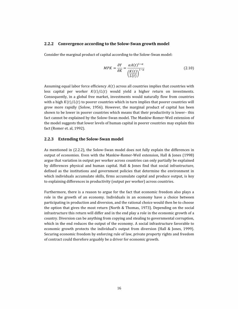
2.2.2 Convergence according to the Solow-Swan growth model
Consider the marginal product of capital according to the Solow-Swan model:
𝑀𝑃𝐾 =𝜕𝑌
𝜕𝐾=
𝛼𝐴(𝑡)1−𝛼
(𝐾(𝑡)𝐿(𝑡)
)1−𝛼 (2.10)
Assuming equal labor force efficiency 𝐴(𝑡) across all countries implies that countries with
less capital per worker 𝐾(𝑡)/𝐿(𝑡) would yield a higher return on investments.
Consequently, in a global free market, investments would naturally flow from countries
with a high 𝐾(𝑡)/𝐿(𝑡) to poorer countries which in turn implies that poorer countries will
grow more rapidly (Solow, 1956). However, the marginal product of capital has been
shown to be lower in poorer countries which means that their productivity is lower– this
fact cannot be explained by the Solow-Swan model. The Mankiw-Romer-Weil extension of
the model suggests that lower levels of human capital in poorer countries may explain this
fact (Romer et. al, 1992).
2.2.3 Extending the Solow-Swan model
As mentioned in (2.2.2), the Solow-Swan model does not fully explain the differences in
output of economies. Even with the Mankiw-Romer-Weil extension, Hall & Jones (1998)
argue that variation in output per worker across countries can only partially be explained
by differences physical and human capital. Hall & Jones find that social infrastructure,
defined as the institutions and government policies that determine the environment in
which individuals accumulate skills, firms accumulate capital and produce output, is key
to explaining differences in productivity (output per worker) across countries.
Furthermore, there is a reason to argue for the fact that economic freedom also plays a
role in the growth of an economy. Individuals in an economy have a choice between
participating in production and diversion, and the rational choice would then be to choose
the option that gives the most return (North & Thomas, 1973). Depending on the social
infrastructure this return will differ and in the end play a role in the economic growth of a
country. Diversion can be anything from copying and stealing to governmental corruption,
which in the end reduces the output of the economy. A social infrastructure favorable to
economic growth protects the individual’s output from diversion (Hall & Jones, 1999).
Securing economic freedom by enforcing rule of law, private property rights and freedom
of contract could therefore arguably be a driver for economic growth.

17
2.3 Composing the linear regression model
2.3.1 Assumptions
This paper examines the assumed key drivers of economic growth using linear regression
based on the Solow model and its extensions, as described in section 2.2. From this
framework the following assumptions are made:
- Economic growth is assumed to change exogenously.
- The depreciation rate of capital 𝛿 and the technological progress g are constant
and exogenous. They can therefore be excluded from the model.
- Savings is assumed to be identical with investments. Investments can come from
both foreign and domestic sources.
- Human capital is assumed to be essential in order to increase productivity from
technological progress.
- Social infrastructure is assumed to be of importance to the output of an economy
and will therefore be included in the model.
2.3.2 Identifying the key drivers of economic output and growth
Based on the theoretical framework presented in this chapter economic output can be
expressed as a function of four variables:
𝑌(𝑡) = 𝐹(𝐾(𝑡), 𝐴(𝑡)𝐿(𝑡), 𝑆(𝑡), 𝐻(𝑡)) (2.11)
𝐾(𝑡) = 𝐶𝑎𝑝𝑖𝑡𝑎𝑙 𝑠𝑡𝑜𝑐𝑘
𝐴(𝑡)𝐿(𝑡) = 𝐸𝑓𝑓𝑖𝑐𝑖𝑒𝑛𝑡 𝑙𝑎𝑏𝑜𝑟 𝑓𝑜𝑟𝑐𝑒
𝑆(𝑡) = 𝑆𝑜𝑐𝑖𝑎𝑙 𝑖𝑛𝑓𝑟𝑎𝑠𝑡𝑟𝑢𝑐𝑡𝑢𝑟𝑒
𝐻(𝑡) = 𝐻𝑢𝑚𝑎𝑛 𝑐𝑎𝑝𝑖𝑡𝑎𝑙
When composing the regression model one needs to consider not only which factors that
drive economic output and growth but also what can be quantified and measured in order
to describe these factors. Furthermore, these measures are chosen so that they are of
analytical value when comparing results with research in the same field. The following
assumptions are derived from the theory presented in chapter 2 and will act as a
foundation for the choice of variables later presented in the methodology section:
- The capital stock 𝐾(𝑡) grow with investments both from foreign and domestic
sources.
- Human capital 𝐻(𝑡) grow with the education level of the population.
- The efficient labor force 𝐴(𝑡)𝐿(𝑡) depends on the health conditions, educational
level and the growth of the population.
- Social infrastructure 𝑆(𝑡) can be described with a measure of economic freedom.

18
The latter assumption is directly aligned with the purpose of this thesis and a condition
for the models that we construct.
2.3.3 GDP growth rate or GDP level?
Relatively recent studies in this field have suggested that in order to capture the long term
differences in economic development one should investigate the levels of GDP rather than
the growth rate. The first argument is that levels gives a better picture of the long term
economic performance which is directly relevant to the welfare of a nation (Hall & Jones,
1996).
The second argument is that Easterly, Kremer, Pritchett and Summers (1993) find little
correlation for economic growth across decades, which in turn proposes that growth rates
are passing and therefore not indicative of long term economic performance (Hall & Jones,
1996).
The final argument is that models advocated by researchers such as Barro & Sala-I-Martin
(1995), Parente & Prescott (1994) and Eaton and Kortum (1995) point towards that
growth rates across countries will in the long run grow at the same rate in accordance
with neoclassical theory.
However, most studies conducted in this field of research have used economic growth rate
as response variable and therefore there is a reason to use it for us as well – for the sake of
comparability. In order to both capture long term economic and short-term economic
performance we will conduct regressions for both response variables

19
3 Regression analysis
The following mathematical framework is primarily based on a literature study of two
titles: Econometrics (Hansen B, 2014) and Elements of regression analysis (Lang H, 2014).
Complementary literature by Studenmund (2006), Heij & de Boer (2004) and Jacoby
(2005) are used to explain a few certain methods: VIF-analysis, Breusch-Pagan test and
Robust regression.
3.1 Linear regression
For a given data set of n observations
{𝑦𝑖 , 𝑥𝑖1, … , 𝑥𝑖𝑘}𝑖=1𝑛 (3.1)
the linear regression model takes the following form:
𝑦𝑖 = ∑ 𝑥𝑖𝑗𝛽𝑗 + 𝑒𝑖
𝑘
𝑗=1
𝑖 = 1, … , 𝑛 (3.2)
This describes the assumed linear relationship between 𝑦𝑖 (dependent variable, or
response variable) and 𝑥𝑖1, … , 𝑥𝑖𝑘 (independent variables, or covariates). Estimates
�̂�1, … , �̂�𝑘 corresponding to the parameters 𝛽1, … , 𝛽𝑘 are obtained by the Ordinary Least
Squares method, explained in section 3.2.
In most cases there is an affine relationship between 𝑥 and y, i.e. one of the covariates is a
constant. By letting the first 𝑥𝑖 be 𝑥𝑜 = 1 the intercept 𝛽0 will determine the size of this
constant.
Equation (3.2) can be written in matrix notation:
𝑌 = 𝑋𝛽 + 𝑒 (3.3)
With the intercept included the first column of the 𝑋 matrix will be filled with ones. The 𝛽
vector now goes from 𝑗 = 0,1,2, … , 𝑘. Since the number of observations are the same
regardless of the intercept’s inclusion, vectors 𝑌 and 𝑒 remain unaltered.
𝑌 = [
𝑦1
𝑦2
⋮𝑦𝑛
] , 𝑋 = [
1 𝑥11 … 𝑥1𝑘
1 𝑥21 … 𝑥11
⋮ ⋮ ⋱ ⋮1 𝑥𝑛1 … 𝑥𝑛𝑘
] , 𝛽 = [
𝛽0
𝛽1
⋮𝛽𝑘
] , 𝑒 = [
𝑒1
𝑒2
⋮𝑒𝑛
] (3.4)

20
As seen above, the linear regression model includes an unobserved random variable 𝑒𝑖
(error term or residual) which represents noise in the relationship between the response
variable and the covariates.
Two assumptions are made:
𝐸(𝑒| 𝑋 ) = 0 (3.5)
𝐸(𝑒2| 𝑋 ) = 𝜎2 (3.6)
In addition, the residuals 𝑒𝑖 are assumed to be independent. In statistics, the sum of
squared residuals are often of interest when analyzing the accuracy of a model. This sum
is defined:
𝑠𝑠𝑒 = ∑ ê𝑖2
𝑛
𝑖=1
= ∑(𝑦𝑖 − �̅�)2
𝑛
𝑖=1
− ∑(�̂�𝑖 − �̅�)2
𝑛
𝑖=1
(3.7)
Where �̂� is a prediction of y and �̅� is the mean value of all observed 𝑦𝑖 ’s.
The standard deviations of the estimates of �̂�𝑗 are obtained through the covariance matrix
𝐶𝑜𝑣(𝛽|𝑋) = (𝑋𝑇𝑋)−1𝜎2 (3.8)
Taking the square root of a diagonal element of the matrix in (10) will return the standard
deviation 𝑆𝐸(𝛽𝑗) of the corresponding 𝛽𝑗 .
Another important concept is the degrees of freedom. Simply put, it is the number of
values in a calculation that are free to vary. For linear regression it is defined as follows:
𝑑𝑓 = 𝑛 − 𝑘 − 1 (3.9)
where 𝑛 is the number of observations and 𝑘 is the number of covariates, intercept not
included. Increasing the number of observations in relation to the number of covariates
will increase the degrees of freedom.
3.2 Ordinary least squares (OLS)
The best linear estimation for regression analysis is Linear Least Squares, often referred
to as Ordinary Least Squares (OLS). By minimizing the sum of squared residuals predicted
by the linear approximation the estimated regression coefficients �̂� are obtained:
𝑒 = 𝑌 − 𝑋𝛽 (3.10)

21
𝑚𝑖𝑛 {𝑓(𝛽) = ∑ 𝑒2
𝑛
𝑖=1
= (𝑌 − 𝑋𝛽)𝑇(𝑌 − 𝑋𝛽)} (3.11)
The Hessian is the identity matrix, thus positive definite and 𝑓(𝛽) is a quadratic function.
=> The objective function is strictly convex
The normal equations 𝑋𝑇ê = 0 yields:
�̂� = (𝑋𝑇𝑋)−1𝑋𝑇𝑌 (3.12)
which is a unique global minimizer for 𝑓(𝛽).
Note that 𝐸(𝛽|𝑋) = �̂�.
3.3 Assumptions
In order to obtain accurate and consistent results from the regression analysis, the
following assumptions must be fulfilled. Potential remedies for eventual transgressions of
assumptions will be presented in the section following this one.
3.3.1 Homoskedasticity
The homoskedasticity assumption is central to linear regression models. By the Gauss-
Markov theorem it ensures that each least-squares estimator is the best linear unbiased
estimator. The assumption states that all the variances of the error terms are constant and
do not depend on the covariates, which in turn means that each probability distribution of
the response variable has the same variance regardless of the covariates. Mathematically,
this is expressed as follows:
𝐸(𝑒|𝑋) = 0
𝐸(𝑒2|𝑋) = 𝜎2 =>
𝑉𝑎𝑟(𝑒|𝑋) = 𝐸(𝑒2|𝑋) − 𝐸(𝑒|𝑋)2 = 𝜎2 (3.13)
3.3.2 Linear independence
The covariates are assumed to be linearly independent, i.e. the correlations between the
covariates are assumed to be zero.
𝐶𝑜𝑟𝑟(𝑥𝑗 , 𝑥𝑖) = 0 <=> 𝐶𝑜𝑣(𝑥𝑗 , 𝑥𝑖) = 0 (3.14)
∀ 𝑖 = 1,2, … , 𝑘 ,
∀ 𝑗 = 1,2, … , 𝑘, 𝑗 ≠ 𝑖
22
3.3.3 Exogeneity
The exogeneity assumption states that the covariates are non-correlated with the error
term such that:
𝐸(𝑒) = 0 (3.15)
3.4 Transgressions of assumptions
The following is a presentation of conditions that may cause transgressions of the above
stated assumptions and the remedies to get around them.
3.4.1 Heteroskedasticity
Whenever assumption (3.3.1) is transgressed the model is considered to heteroskedastic
– the response variable’s observed values can no longer be assumed to be outcomes from
the same probability distribution. Breaking this assumption implies breaking the Gauss-
Markov theorem and which means that the least-squares estimates are no longer
considered to be the best linear unbiased estimators. This becomes a practical issue when
performing F-tests.
The Breusch-Pagan test can be used in order to determine the probability that a given
model suffers from heteroskedasticity - this method is explained in section 3.11.
In order to avoid heteroskedasticity one might consider revising the model at hand by
transforming variables in such a manner that the differences in variance becomes smaller.
If heteroskedasticity cannot be avoided, robust regression methods may provide an
alternative to least squares estimation. Robust regression will be further explained in
section 3.12.
3.4.2 Multicollinearity
If assumption 3.3.2 is transgressed then two or more covariates are correlated. This
phenomenon is called multicollinearity and can be a problem depending on to which
degree the covariates are correlated. In the case of perfect multicollinearity one or more
covariates can be expressed as a linear combination of other covariates. Consequently the
matrix 𝑋 will be singular and the normal equations will not produce a unique solution. In
this case, the only remedy is to remove one of the covariates so that the matrix 𝑋 is no
longer singular.
A high degree of multicollinearity (near perfect multicollinearity) will produce large
standard errors. This can be avoided by having a large number of observations in relation
to the number of covariates so that the size of the unbiased variance estimator is reduced.

23
𝑠2 =𝜎2
𝑛 − 𝑘 − 1 (3.16)
The variance inflation factor (VIF) provides a way to quantify the severity of
multicollinearity and will be further explained in section 3.11.
3.4.3 Endogeneity
If a covariate is correlated with the error term it implies that a correlation coefficient in
the OLS regression is biased and will not produce consistent estimates. Endogeneity can
have its explanation in the following common problems and can easily be proven.
Omitted variable(s)
Consider the following two models where 𝑧𝑖 is the omitted variable:
𝑦𝑖 = 𝛼 + 𝛽𝑥𝑖 + 𝛾𝑧𝑖 + 𝑒𝑖 (3.17)
𝑦𝑖 = 𝛼 + 𝛽𝑥𝑖 + 휀𝑖 (3.18)
𝑤ℎ𝑒𝑟𝑒 휀𝑖 = 𝛾𝑧𝑖 + 𝑒𝑖 𝑎𝑛𝑑 𝛾 ≠ 0
If correlation exists between included variables 𝑥𝑖 and omitted variable 𝑧𝑖 , and 𝑧𝑖
separately affects 𝑦𝑖 (which is the case in equation 3.17), then 𝑥𝑖 correlates with the error
term 휀𝑖. Then, in the second equation, 𝐶𝑜𝑟𝑟(𝑥𝑖 , 휀𝑖) ≠ 0, thus 𝑥𝑖 is endogenous.
Measurement errors
Consider the following regression:
𝑦 = 𝛽 + 𝛾𝑥 + 𝜖 (3.19)
Let �̃� = 𝑥 + 휀 where 𝑥 is the ”true” value of �̃� and 휀 is the measurement error. The
regression now becomes:
𝑦 = 𝛽 + 𝛾(�̃� − 휀) + 𝜖 = 𝛽 + 𝛾(�̃� − 휀) + 𝜖 =
= 𝛽 + 𝛾�̃� + 𝜖 − 𝛾휀 = 𝛽 + 𝛾�̃� + �̃� (3.20)
𝑖. 𝑒. 𝐶𝑜𝑟𝑟(�̃�, 휀 ) ≠ 0, 𝑡ℎ𝑢𝑠 𝑒𝑛𝑑𝑜𝑔𝑒𝑛𝑜𝑢𝑠
Simultaneity
Consider the following two equations:
𝑦𝑖 = 𝛽1𝑥𝑖 + 𝛾1𝑧𝑖 + 𝑢𝑖 (3.21)
𝑧𝑖 = 𝛽2𝑥𝑖 + 𝛾2𝑧𝑖 + 𝑣𝑖 (3.22)

24
Solving for 𝑧𝑖 yields the following:
𝑧𝑖 =(𝛽2 + 𝛾2𝛽1)𝑥𝑖 + 𝑣𝑖 + 𝛾2𝑢𝑖
1 − 𝛾1𝛾2
(3.23)
Given that 𝐶𝑜𝑟𝑟(𝑥𝑖 , 𝑢𝑖) = 𝐶𝑜𝑟𝑟(𝑣𝑖 , 𝑢𝑖) = 0 and 1 − 𝛾1𝛾2 ≠ 0:
𝐶𝑜𝑣(𝑧𝑖 , 𝑢𝑖) = 𝐸(𝑧𝑖𝑢𝑖) =𝛾2
1 − 𝛾1𝛾2
𝐸(𝑢𝑖𝑢𝑖) ≠ 0 (3.24)
𝑧𝑖 is correlated with the error term 𝑢𝑖 , thus endogenous.
If the model is proven to be endogenous, an implementation of instrumental variables and
a two stage least square linear regression can be appropriate. Instrumental variables are
variables that correlate with the endogenous variable but not with the residual
(exogenous variables). If it is shown to be difficult to find these variables one might
consider revising the model or simply acknowledge the bias problem.
3.7 Hypothesis testing (F-test)
In statistical analysis it is common to test different hypotheses. A null hypothesis is stated:
𝐻0: 𝛽𝑗 = 𝛽𝑗0 (3.25)
A common null hypothesis is to test whether there is any relationship at all between the
response variable and a certain covariate. No relationship between 𝑦 and 𝑥𝑗 is equivalent
to 𝛽𝑗 = 0:
𝐻0: 𝛽𝑗 = 𝛽𝑗0 = 0 (3.26)
To perform a F-test you compute the F statistic:
𝐹 = (�̂�𝑗 − 𝛽𝑗
0
𝑆𝐸(�̂�𝑗))
2
(3.27)
Assuming homoskedasticity, the F-statistic is exact. The F-statistic is then used to compute
the p-value. The p-value denotes the probability of the observed outcome, given the
hypothesis is true. It is defined as:
𝑝 = 𝑃(𝑋 > 𝐹) (3.28)

25
Where 𝑋 is some 𝐹𝛼(1, 𝑑𝑓)-distributed random variable for a chosen risk level 𝛼. If 𝑝 < 𝛼
we reject 𝐻0. If 𝑝 > 𝛼, we cannot reject 𝐻0.
For structural interpretation the confidence interval of 𝛽𝑗 is computed as follows:
�̂�𝑗 ± √𝐹𝛼(1, 𝑑𝑓)𝑆𝐸(�̂�𝑗) (3.29)
where 𝐹𝛼 is the quantile of the F-distribution for a chosen level of significance 𝛼,
commonly one, five or ten percent. The confidence interval gives a clear view of which
values the estimate �̂�𝑗 could plausibly assume for the chosen significance level. If the
confidence interval of 𝛽𝑗 spans over zero, the corresponding covariate 𝑥𝑗 may be
insignificant in the regression model (more on this in section 3.7).
3.8 Transformation of variables
Whenever a covariate and the response variable has a non-linear relationship a
transformation is appropriate in order to get accurate results from the OLS linear
regression. Below is the description of a commonly used transformation: exponential
transformation.
3.8.1 Exponential transformation
Assume that the covariates 𝑋 and the response variable Y has a exponential relationship
such that 𝑦𝑖 = 𝑒𝑥𝑖 an appropriate transformation would be from
Y = 𝛽𝑋 + 𝑒 (3.30)
To
ln(𝑌) = 𝛽𝑋 + 𝑒 (3.31)
A change in X will now imply a relative change Y.
3.9 Coefficient of determination (𝑹𝟐)
𝑅2 is a measure of how well the data fits the statistical model – or reversely: how well the
model can replicate observed outcomes. The 𝑅2 number takes values between 0 and 1. A
high 𝑅2 is in general good, but does not necessarily imply that the model is correct. The 𝑅2
is calculated as

26
𝑅2 = 1 −𝑠𝑠𝑒
𝑠𝑠𝑡𝑜𝑡
(3.32)
Where 𝑠𝑠𝑒 is the sum of squared residuals as defined by equation (7). The total sum of
squares, 𝑠𝑠𝑡𝑜𝑡 , is defined as
𝑡𝑠𝑠 = ∑(𝑦𝑖 − �̅�)2
𝑛
𝑖=1
(3.33)
Since OLS minimizes 𝑠𝑠𝑒 it follows that it maximizes 𝑅2. The total sum of squares stays the
same regardless of estimation method.
An alternative way to compute 𝑅2 is the following:
𝑅2 =|𝑒∗|2 − |𝑒|2
|𝑒∗|2 (3.34)
Where 𝑒∗ denotes the residual of a restricted regression model (with only an intercept). 𝑒
denotes the residual of the unrestricted model (no covariates excluded).
A well-known shortcoming of the 𝑅2 measure is that is increases when more covariates
are included, regardless of their significance. Because of this there is a similar measure
which penalizes complexity - adjusted 𝑅2:
𝑅𝑎𝑑𝑗2 = 1 −
𝑛 − 1
𝑛 − 𝑘 − 1(1 − 𝑅2) (3.35)
Where 𝑛 denotes the number of observations and 𝑘 denotes the number of covariates.
Unlike 𝑅2, the 𝑅𝑎𝑑𝑗2 will only increase if an added variable adds explanatory value to the
model.
3.10 Akaike information criterion (AIC)
The Akaike information criterion is a useful tool for model selection. It is based on the
likelihood function and ranks regression models with a score, where a lower value is
better. Regression models are penalized for a) large expected errors, and b) complexity
(more covariates than necessary). The AIC is computed as:
𝐴𝐼𝐶 = 𝑛 ∗ ln(𝑠𝑠𝑒) + 2 ∗ (𝑘 + 1) (3.36)
Where 𝑛 is the number of observations and 𝑘 is the number of covariates (intercept not
included).

27
A regression model can be stepwise reduced by computing the AIC for each combination
of the model where one covariate is left out. The model is in each step be reduced such
that the AIC score is minimized.
3.11 Variance inflation factor (VIF)
The variance inflation factor (VIF) can be used to quantify the severity of multicollinearity.
It is calculated for each covariate 𝑥𝑖 by running a regression with 𝑥𝑖 as response variable
and the remaining covariates as independent variables. A good fit indicates that the
regressand and the regressors contain nearly the same information, or in other words:
there is a high degree of multicollinearity. The VIF for each covariate 𝑥𝑖 is calculated as:
𝑉𝐼𝐹𝑖 =1
1 − 𝑅𝑖2 (3.37)
where 𝑅𝑖2 is the coefficient of determination (explained in section 3.9) for the respective
regression. By rule of thumb, a VIF value exceeding 10 is regarded as a sign of severe
(near-perfect) multicollinearity.
3.12 Breusch-Pagan test
The Breusch-Pagan test is used to test a linear regression model for conditional
heteroskedasticity. Breusch-Pagan tests for heteroskedasticity by testing whether the
estimated variance of the residuals are dependent on the covariates. This is done by
running an auxiliary regression with the residuals-squared as response variable. The test
statistic
𝐿𝑀 = 𝑛𝑅2 (3.38)
𝑛 = 𝑠𝑎𝑚𝑝𝑙𝑒 𝑠𝑖𝑧𝑒
𝑅2 = 𝑐𝑜𝑒𝑓𝑓𝑖𝑐𝑖𝑒𝑛𝑡 𝑜𝑓 𝑑𝑒𝑡𝑒𝑟𝑚𝑖𝑛𝑎𝑡𝑖𝑜𝑛 𝑜𝑓 𝑡ℎ𝑒 𝑎𝑢𝑥𝑖𝑙𝑖𝑎𝑟𝑦 𝑟𝑒𝑔𝑟𝑒𝑠𝑠𝑖𝑜𝑛
is then asymptotically 𝜒2(𝑘 − 1)-distributed under the null hypothesis of
homoskedasticity, where k denotes the number of covariates.
3.13 Robust regression models
When the homoskedasticity assumption does not hold, the OLS estimate is at risk of being
biased by outliers, i.e. the estimate will no longer be representative to a majority of the
observations. If this cannot be avoided by model revision, robust models can provide an

28
alternative to OLS. Robustness in this context means that the model has the following
features:
- Unbiased and (reasonably) efficient.
- Minor transgressions of the model assumptions will not have a major impact on
the performance of the model.
- Major transgressions of the model assumptions will not invalidate the model
completely.
OLS is not robust to outliers. One way to increase robustness is to alter the objective
function. The perhaps simplest change is to minimize Least Absolute Values (LAV) of
errors instead of the least squares (OLS). LAV reduces the influence from heavy outliers
but is less efficient and less reliable than OLS near the center of the distribution. More
sophisticated methods include M-estimators such as the Huber objective function, which
behaves like OLS near the center of the distribution and like LAV at extreme observations:
𝜌𝐻(𝑒) = {
1
2𝑒2 𝑓𝑜𝑟 𝑒 ≤ 𝑘
𝑘|𝑒| −1
2𝑘2 𝑓𝑜𝑟 𝑒 > 𝑘
(3.39)
Where 𝑘 denotes the tuning constant. A smaller 𝑘 gives more resistance to outliers at the
expense of efficiency for observations within normality.
Another way to handle outliers is to assign weights for each error, giving greater influence
to small errors than for large errors. The Huber weight function is defined as follows:
𝑤(𝑒) = {
1 𝑓𝑜𝑟 |𝑒| > 𝑘𝑘
|𝑒|𝑓𝑜𝑟 |𝑒| ≤ 𝑘
(3.40)
By assigning weights to residuals, a robust estimation can be obtained by minimizing the
weighted sum of squares:
∑ 𝑤𝑖2𝑒𝑖
2
𝑛
𝑖=1
(3.41)
Since the weights 𝑤𝑖 are dependent on the residuals in the model, they cannot be
computed until we know the residuals themselves – i.e. we cannot compute them until
after fitting an initial regression. Finding the best estimate through weighted residuals
requires an iterative solution, where the residuals gets reweighted in each iteration. The
process stops when the slope coefficients (the 𝛽 estimates) converge. This process is
called Iterative Reweighted Least Squares (IRLS).
In this thesis, the R function lmRob in the Robust package is used to perform robust
regressions. It is based on the same principles as described above.

29
4 Quantitative methodology
4.1 Response variable
Regressions are run on two individual response variables:
GDP/capita (constant 2005 US$) – GDPc
Calculated as the aggregated value added by domestic producers, plus product taxes, minus
subsidies, divided by midyear population. Data are in constant 2005 USD.
GDP/capita growth (annual %) – GDPcg
Calculated as the percentage increase (or decrease) in GDP/capita (constant 2005 US$)
from one year to another. The percentage for each year is obtained by dividing the current
year GDP/capita with that of the prior year.
4.2 Covariates
Initial GDP per capita – GDPi
GDP/capita level as of 2000, the first year of the observed period. Data are expressed in
constant 2005 USD.
Gross Domestic Investment – GDI
Calculated as total investments in fixed assets plus net change in inventory levels,
including “work in progress” production. Also known as gross capital formation. Values
are expressed in percentage of total GDP.
Economic Freedom – Ecfree
Score in the “Index of Economic Freedom”, compounded by Heritage Foundation. The
index scores each country based on 10 qualitative and quantitative factors in four
categories:
1. Rule of Law (property rights, freedom from corruption).
2. Limited Government (fiscal freedom, government spending).
3. Regulatory Efficiency (business freedom, labor freedom, monetary freedom).
4. Open markets (trade freedom, investment freedom, financial freedom).

30
Foreign Direct Investment – FDI
Calculated as annual net inflows from foreign investors to acquire 10% or more of the
voting stock in an enterprise operating in the country. Values are expressed in percentage
of total GDP.
Population growth – Popg
Calculated as the annual percentage increase in mid-year measured population.
Education – Educ
Average years of schooling for population (males and females) aged 25 and older.
Life expectancy – Lifexp
Number of years a newborn infant is expected to live, given the country’s current
mortality patterns remain throughout the child’s life.
Dummy variables – 2009, 2010
Denotes years 2009 and 2010.
4.2.1 Covariate scaling
Each covariate is scaled to a normalized version by subtracting the mean and dividing by
its standard deviation. This leads to a corresponding change in scale of coefficients and
standard errors but has no effect on the significance or the interpretation of the variable.
Scaling covariates allows us to compare the sizes of coefficients of significant covariates.
𝑥𝑠 =𝑥 − �̅�
𝜎 (4.1)
4.3 Data
Data for years 2000-2013 are collected from three sources:
World Bank
GDP/capita, GDP/capita growth, initial GDP/capita, GDI, FDI, GDP/capita, inflation,
population growth, fertility rate, life expectancy.

31
Barro-Lee dataset
Education.
Heritage Foundation
Economic Freedom.
4.3.1 Adjustments on data
Countries consistently lacking data in several categories are consciously excluded. Where
only a few data points are lacking, linear extrapolation is used to synthesize values
coherent to the general trend. Data are synthesized to a greater extent on the Barro-Lee
dataset on educational attainment, which only contains data on a five year basis. To deal
with this, annual values are set equal to the values of the first year of each five year
interval, i.e. values for years 2001-2004 are set equal to the value of year 2000, and so on.
4.3.2 Source criticism
We expect data from all of our sources to be affected by measurement errors. The datasets
rely on information from official sources and measurement errors are attempted to be
adjusted for. However, different countries have different ways of measuring and the
reliability is in some cases in question – we recognize this issue and expect impact in form
of endogeneity in our models as a result.
The Barro-Lee dataset on education are produced with a few assumptions and data
adjustments. These include forward and backward extrapolation to fill in missing
observations, as well as an assumption of educational attainment remaining unchanged
from age 25 to 64. This assumption may not always hold true, especially in advanced
economies where many individuals finish their educations at a later age than 25.
Furthermore, Barro & Lee’s breakdown of four levels of schooling (no school, primary
school, secondary school and higher education) may not perfectly reflect the situation in
each country, since the educational systems can widely differ between countries. On the
basis that the Barro-Lee dataset has been widely used in previous research on several
topics, including GDP regressions, it is assumed to be trustworthy. According to the
Journal of Development Economics, where the latest version of the data (2013) was
published, the dataset has been cited over 1700 times in research articles.
The measure on economic freedom is arguably also a source of error. Since there is no
universally accepted definition of economic freedom, an objective measure cannot be
defined. The measure used in this thesis, the Index of Economic Freedom is a scoring
based on qualitative and quantitative measures selected by Heritage Foundation in
cooperation with Wall Street Journal. Heritage Foundation is an American conservative
think tank with the outspoken mission to promote conservative public policies. This
32
imposes a risk of unfair scores due to a conservatively biased view on what economic
freedom really is. However, De Haan & Sturm (1999) compare this index with another
measure: Economic Freedom Index compounded by independent Canadian think tank
Fraser Institute, reaching the conclusion that the two indices, while having their
differences, rank the countries similarly. Based on this we do not consider the index to be
biased to a troublesome extent.
4.4 Initial regression models
Regressions are run on two panels of countries:
Developing countries
25 countries falling under the 2014 IMF classification of developing countries. Denoted
with superscript u- in regression model expressions.
Developed countries
25 countries falling under the 2014 IMF classification of developed countries. Denoted
with superscript d- in regression model expressions.
4.4.1 GDP/capita level regression model
log(𝐺𝐷𝑃𝑐) = 𝛽0 + 𝛽1𝐺𝐷𝐼 + 𝛽2𝐹𝐷𝐼 + 𝛽3𝑃𝑜𝑝𝑔 + 𝛽4𝐸𝑑𝑢𝑐 + 𝛽5𝐿𝑖𝑓𝑒𝑥𝑝 + 𝛽6𝐸𝑐𝑓𝑟𝑒𝑒 + 𝑒
The logarithmic transformation of the of the response variable is a measure taken to
stabilize variances in order to avoid issues with heteroskedasticity. This is especially
important when running regressions on a panel with large variations within the sample,
which is the case for the GDP/capita dataset. The largest observed value in this set is
almost 1800 times larger than the smallest value. When logarithmic transformation is
applied, they differ by a factor 2.6. The role of logarithmic transformations in regression
analysis has been subject to extensive discussion, Lütkepohl & Xu (2009) and Caroll &
Ruppert (1988) being two contributions on the matter, concluding that heteroskedasticity
can be reduced using the transformations.
4.4.2 GDP/capita growth regression model
𝐺𝐷𝑃𝑐𝑔 = 𝛾0 + 𝛾1𝐺𝐷𝐼 + 𝛾2𝐹𝐷𝐼 + 𝛾3𝑃𝑜𝑝𝑔 + 𝛾4𝐸𝑑𝑢𝑐 + 𝛾5𝐿𝑖𝑓𝑒𝑥𝑝 + 𝛾6𝐸𝑐𝑓𝑟𝑒𝑒 + 𝛾7𝐺𝐷𝑃𝑖
+ 𝛾82009 + 𝛾92010 + 𝑢
Logarithmic transformation cannot be applied to the response variable, since its data takes negative values.

33
Table 4.4.3.1: Expected signs of
coefficient for the initial regression
on GDP/capita level.
Table 4.4.3.2: Expected signs of
coefficient for the initial regression on
GDP/capita growth rate.
4.4.3 Expected outcome of coefficient estimates
The following expected outcomes of the signs of coefficient estimates are based on a
ceteris paribus argumentation, i.e.:
- All changes in covariate values are assumed to be exogenous.
- Possible effects from changes in one covariate on other covariates are excluded,
thus indirect effects on the response variable are not considered.
- No simultaneity or reverse causalities between the covariates and the response
variable are considered.
Furthermore, no major distinctions are made between economic output and economic
growth; what is favorable to economic growth is assumed to be favorable to economic
output, and vice versa. Short motivations for each covariate are presented in appendix.
Needless to say, these reservations form an oversimplification of reality: the proposed
outcomes below simply form a point of reference from where the discussion in chapter 7
can revolve.
Economic output model Economic growth model
Developing Developed
GDI + +
FDI + +
Popg - -
Educ + +
Lifexp + +
Ecfree + +
Developed Developing
GDI + +
FDI + +
Popg - -
Educ + +
Lifexp + +
Ecfree + +
GDPi - -
2009 - -
2010 - -

34
4.5 Algorithm for model improvement
Starting with the initial regression model, each model is evaluated and revised according to the following flowchart:
Figure 4.5: Model improvement flowchart.
The flowchart in figure 4.5 illustrates the process for model improvement and acts as
guidelines from the initial regression to the final regression. The algorithm accounts for
multicollinearity, heteroskedasticity and the models will be reduced with AIC and/or F-
tests. We assume that Solow-Swan’s assumptions on exogeneity hold and therefore
endogeneity issues are not included in the algorithm for model improvement. Possible
issues with endogeneity biases will be elaborated and discussed in chapter 7.
Note the following:
AIC reductions will be made stepwise until the model with the lowest AIC-value is
found.
Reductions from OLS regression models will consider both results from F-tests
and AIC tests.
Reductions from robust regressions will information produced from F-tests.
No
Yes
No
Formulate regression model
Run regression
VIF-test
Multicollinearity?
Yes
Re-
Breusch-Pagan test
Heteroskedasticity?
Robust regression
Final regression model
AIC F-test

35
If an initial regression is shown to have severe problems with multicollinearity and/or
heteroskedasticity they will not be presented in the result section. The model will be
reformulated or be robustly regressed until the results presented are of analytical value.
36
5 Results for economic output
5.1 Initial regression for economic output in developing
countries
Estimate Std. Error t value Pr(>|t|) Significance level
(Intercept) 7.11951 0.03449 206.409 < 2e-16 ***
Ecfree 0.19887 0.03649 5.450 9.65e-08 ***
GDI 0.23692 0.04102 5.775 1.72e-08 ***
Educ 0.50450 0.04837 10.431 < 2e-16 ***
Lifexp 0.25429 0.04437 5.731 2.19e-08 ***
FDI -0.23754 0.03913 -6.070 3.39e-09 ***
Popg 0.05783 0.05703 1.014 0.311
Significance codes: ‘***’ 0.001, ‘**’ 0.01, ‘*’ 0.05, ‘.’ 0.1.
𝐀𝐝𝐣. 𝐑𝟐 RSE DF
0.5409 0.6453 343
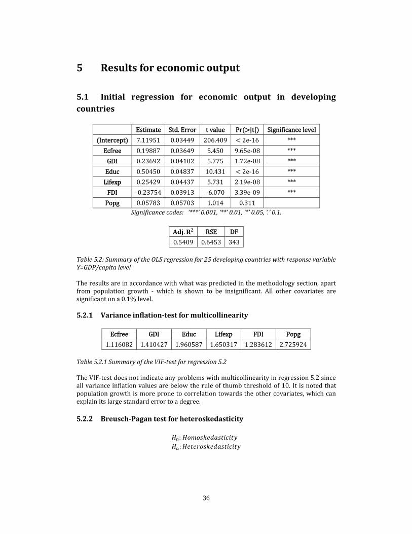
Table 5.2: Summary of the OLS regression for 25 developing countries with response variable Y=GDP/capita level The results are in accordance with what was predicted in the methodology section, apart from population growth - which is shown to be insignificant. All other covariates are significant on a 0.1% level.
5.2.1 Variance inflation-test for multicollinearity
Ecfree GDI Educ Lifexp FDI Popg
1.116082 1.410427 1.960587 1.650317 1.283612 2.725924
Table 5.2.1 Summary of the VIF-test for regression 5.2 The VIF-test does not indicate any problems with multicollinearity in regression 5.2 since all variance inflation values are below the rule of thumb threshold of 10. It is noted that population growth is more prone to correlation towards the other covariates, which can explain its large standard error to a degree.
5.2.2 Breusch-Pagan test for heteroskedasticity
𝐻0: 𝐻𝑜𝑚𝑜𝑠𝑘𝑒𝑑𝑎𝑠𝑡𝑖𝑐𝑖𝑡𝑦
𝐻𝑎: 𝐻𝑒𝑡𝑒𝑟𝑜𝑠𝑘𝑒𝑑𝑎𝑠𝑡𝑖𝑐𝑖𝑡𝑦
37
𝛘𝟐 𝐃𝐟 𝐩 − 𝐯𝐚𝐥𝐮𝐞
1.582337 1 0.2084244
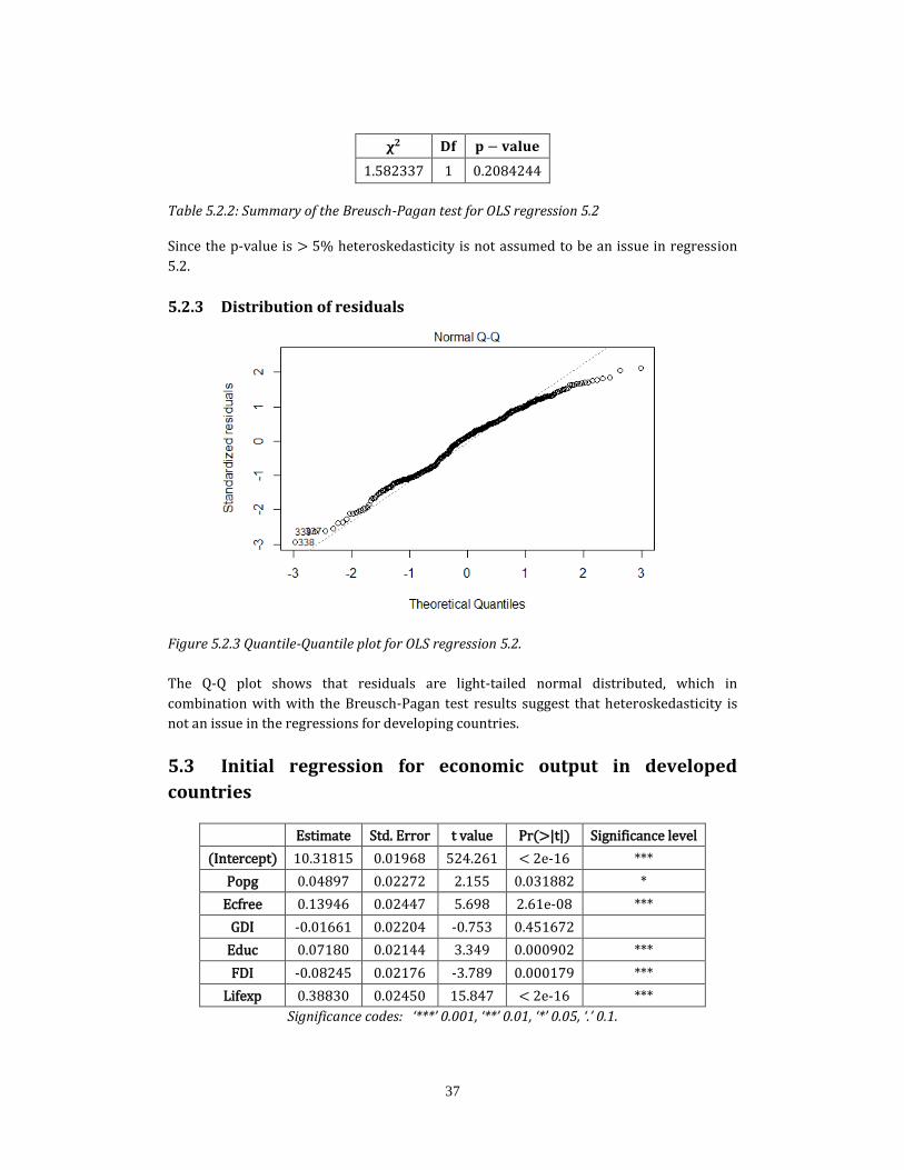
Table 5.2.2: Summary of the Breusch-Pagan test for OLS regression 5.2 Since the p-value is > 5% heteroskedasticity is not assumed to be an issue in regression
5.2.
5.2.3 Distribution of residuals
Figure 5.2.3 Quantile-Quantile plot for OLS regression 5.2.
The Q-Q plot shows that residuals are light-tailed normal distributed, which in
combination with with the Breusch-Pagan test results suggest that heteroskedasticity is
not an issue in the regressions for developing countries.
5.3 Initial regression for economic output in developed
countries
Estimate Std. Error t value Pr(>|t|) Significance level
(Intercept) 10.31815 0.01968 524.261 < 2e-16 ***
Popg 0.04897 0.02272 2.155 0.031882 *
Ecfree 0.13946 0.02447 5.698 2.61e-08 ***
GDI -0.01661 0.02204 -0.753 0.451672
Educ 0.07180 0.02144 3.349 0.000902 ***
FDI -0.08245 0.02176 -3.789 0.000179 ***
Lifexp 0.38830 0.02450 15.847 < 2e-16 ***
Significance codes: ‘***’ 0.001, ‘**’ 0.01, ‘*’ 0.05, ‘.’ 0.1.
38
𝐀𝐝𝐣. 𝐑𝟐 RSE DF
0.6336 0.3677 343
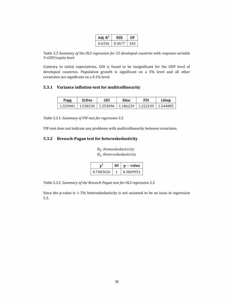
Table 5.3 Summary of the OLS regression for 25 developed countries with response variable Y=GDP/capita level. Contrary to initial expectations, GDI is found to be insignificant for the GDP level of
developed countries. Population growth is significant on a 5% level and all other
covariates are significant on a 0.1% level.
5.3.1 Variance inflation-test for multicollinearity
Popg Ecfree GDI Educ FDI Lifexp
1.329401 1.538230 1.253096 1.186229 1.222239 1.544885
Table 5.3.1: Summary of VIF-test for regression 5.3.
VIF-test does not indicate any problems with multicollinearity between covariates.
5.3.2 Breusch-Pagan test for heteroskedasticity
𝐻0: 𝐻𝑜𝑚𝑜𝑠𝑘𝑒𝑑𝑎𝑠𝑡𝑖𝑐𝑖𝑡𝑦
𝐻𝑎: 𝐻𝑒𝑡𝑒𝑟𝑜𝑠𝑘𝑒𝑑𝑎𝑠𝑡𝑖𝑐𝑖𝑡𝑦
𝛘𝟐 𝐃𝐟 𝐩 − 𝐯𝐚𝐥𝐮𝐞
0.7483626 1 0.3869951
Table 5.3.2: Summary of the Breusch-Pagan test for OLS regression 5.3.
Since the p-value is > 5% heteroskedasticity is not assumed to be an issue in regression
5.3.

39
5.3.3 Distribution of residuals
Figure 5.3.3: Quantile-Quantile plot of initial OLS regression 5.3.
As with the regression on developing countries, the Q-Q plot for developed countries show
that residuals are light-tailed normal distributed, which in combination with the Breusch-
Pagan test suggest that the resiudals are normal distributed and that heteroskedasticity is
not an issue.
5.4 AIC analysis of the initial OLS regressions
5.4.1 Developing countries
Dropped covariate Df Sum of Sq RSS AIC
Popg 1 0.428 143.25 -300.66
None
142.82 -299.71
Ecfree 1 12.367 155.19 -272.64
Lifexp 1 13.675 156.50 -269.71
GDI 1 13.889 156.71 -269.23
FDI 1 15.342 158.17 -266.00
Educ 1 45.307 188.13 -205.28
Table 5.4.1: Summary of the AIC-analysis for regression 5.2.
The AIC-analysis indicates that the population growth covariate should be excluded from
the final model. The difference in AIC is relatively small in comparison to the full model,
40
but since population growth was found to be insignificant in regression 5.2 there is reason
to consider a reduction of the model.
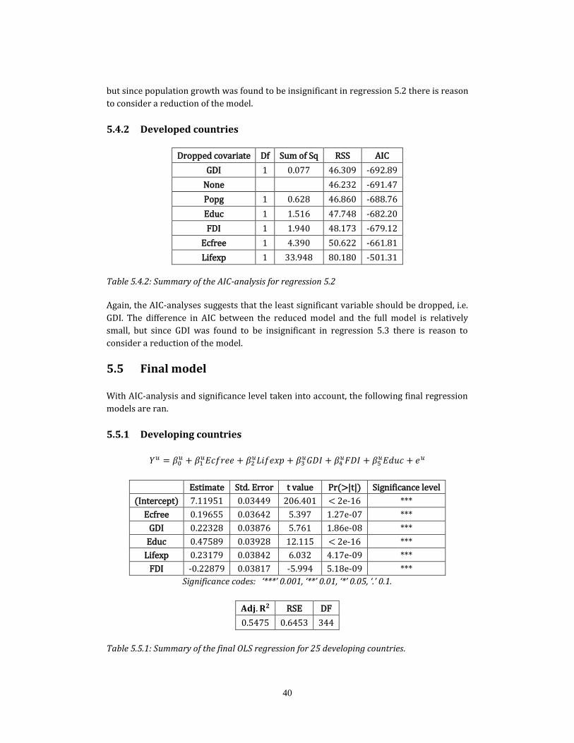
5.4.2 Developed countries
Dropped covariate Df Sum of Sq RSS AIC
GDI 1 0.077 46.309 -692.89
None
46.232 -691.47
Popg 1 0.628 46.860 -688.76
Educ 1 1.516 47.748 -682.20
FDI 1 1.940 48.173 -679.12
Ecfree 1 4.390 50.622 -661.81
Lifexp 1 33.948 80.180 -501.31
Table 5.4.2: Summary of the AIC-analysis for regression 5.2
Again, the AIC-analyses suggests that the least significant variable should be dropped, i.e.
GDI. The difference in AIC between the reduced model and the full model is relatively
small, but since GDI was found to be insignificant in regression 5.3 there is reason to
consider a reduction of the model.
5.5 Final model
With AIC-analysis and significance level taken into account, the following final regression
models are ran.
5.5.1 Developing countries
𝑌𝑢 = 𝛽0𝑢 + 𝛽1
𝑢𝐸𝑐𝑓𝑟𝑒𝑒 + 𝛽2𝑢𝐿𝑖𝑓𝑒𝑥𝑝 + 𝛽3
𝑢𝐺𝐷𝐼 + 𝛽4𝑢𝐹𝐷𝐼 + 𝛽5
𝑢𝐸𝑑𝑢𝑐 + 𝑒𝑢
Estimate Std. Error t value Pr(>|t|) Significance level
(Intercept) 7.11951 0.03449 206.401 < 2e-16 ***
Ecfree 0.19655 0.03642 5.397 1.27e-07 ***
GDI 0.22328 0.03876 5.761 1.86e-08 ***
Educ 0.47589 0.03928 12.115 < 2e-16 ***
Lifexp 0.23179 0.03842 6.032 4.17e-09 ***
FDI -0.22879 0.03817 -5.994 5.18e-09 ***
Significance codes: ‘***’ 0.001, ‘**’ 0.01, ‘*’ 0.05, ‘.’ 0.1.
𝐀𝐝𝐣. 𝐑𝟐 RSE DF
0.5475 0.6453 344
Table 5.5.1: Summary of the final OLS regression for 25 developing countries.

41
In the final model for GDP/capita in developing countries, regression results show
positive correlations, on a 0.1% significance level, for Ecfree, GDI, Educ and Lifexp. FDI is
found to be negatively correlated, also on a 0.1% significance level.
5.5.2 Developed countries
𝑌𝑑 = 𝛽0𝑑 + 𝛽1
𝑑𝐸𝑐𝑓𝑟𝑒𝑒 + 𝛽2𝑑𝐿𝑖𝑓𝑒𝑥𝑝 + 𝛽3
𝑑𝐹𝐷𝐼 + 𝛽4𝑑𝐸𝑑𝑢𝑐 + 𝛽5
𝑑𝑃𝑜𝑝𝑔 + 𝑒𝑑
Estimate Std. Error t value Pr(>|t|) Significance level
(Intercept) 10.31812 0.01967 524.591 < 2e-16 ***
Popg 0.04513 0.02213 2.039 0.042214 *
Ecfree 0.13721 0.02428 5.652 3.34e-08 ***
Educ 0.07303 0.02136 3.418 0.000706 ***
FDI -0.08480 0.02153 -3.939 9.90e-05 ***
Lifexp 0.39560 0.02249 17.590 < 2e-16 ***
Significance codes: ‘***’ 0.001, ‘**’ 0.01, ‘*’ 0.05, ‘.’ 0.1.
𝐀𝐝𝐣. 𝐑𝟐 RSE DF
0.6393 0.3674 344
Table 5.5.2: Summary of the final OLS regression for 25 developed countries.
In the final model for GDP/capita in developed countries, regression results show positive
correlations for population growth, economic freedom, education and life expectancy. FDI
is found to be negatively correlated with GDP/capita. All covariates are significant on a
0.1% level, except for population growth which is significant on a 5% level.
5.6 Economic output and economic freedom
The following page shows plots on one of the relationships of main interest in this thesis:
economic freedom and economic output.
42
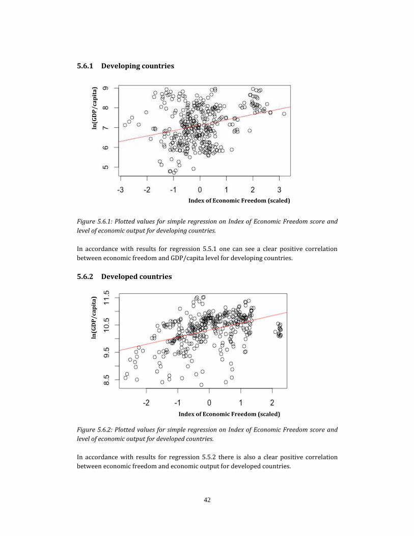
5.6.1 Developing countries
Figure 5.6.1: Plotted values for simple regression on Index of Economic Freedom score and
level of economic output for developing countries.
In accordance with results for regression 5.5.1 one can see a clear positive correlation
between economic freedom and GDP/capita level for developing countries.
5.6.2 Developed countries
Figure 5.6.2: Plotted values for simple regression on Index of Economic Freedom score and
level of economic output for developed countries.
In accordance with results for regression 5.5.2 there is also a clear positive correlation
between economic freedom and economic output for developed countries.
Index of Economic Freedom (scaled)
ln(G
DP
/ca
pit
a)
ln(G
DP
/ca
pit
a)
Index of Economic Freedom (scaled)

43
6 Results for economic growth
As shown in section 6.2, there is presence of heteroskedasticity in the regression model
for annual GDP/capita growth. This causes OLS estimation to be inefficient and its results
to be unreliable. Those coefficient OLS estimates are therefore of no use and will not be
presented.
6.1 Diagnosing for multicollinearity
VIF calculations on initial OLS regressions, presented below, show no signs of severe
multicollinearity. This means that no model reformulations have to be made and that the
model improvement process can proceed according to the flowchart in section 4.5.
6.1.1 Initial OLS for developing countries
GDPi Popg Ecfree GDI Educ FDI Lifexp 2009 2010
1.7742 2.9763 1.5144 1.4526 1.9684 1.3521 1.6734 1.0073 1.0112
Table 6.1.1: Summary of VIF-test for OLS regression on annual GDP/capita growth in
developing countries.
We note that population growth has largest VIF-value and is therefore more prone
towards multicollinearity than any of the other covariates.
6.1.2 Initial OLS for developed countries
GDPi Popg Ecfree GDI Educ FDI Lifexp 2009 2010
1.8434 1.3404 1.6767 1.3297 1.1951 1.2438 1.9105 1.0226 1.0266
Table 6.1.2: Summary of VIF-test for OLS regression on annual GDP/capita growth in
developed countries.
All covariates have relatively low VIF-values, meaning multicollinearity is unlikely to be
causing any problems.
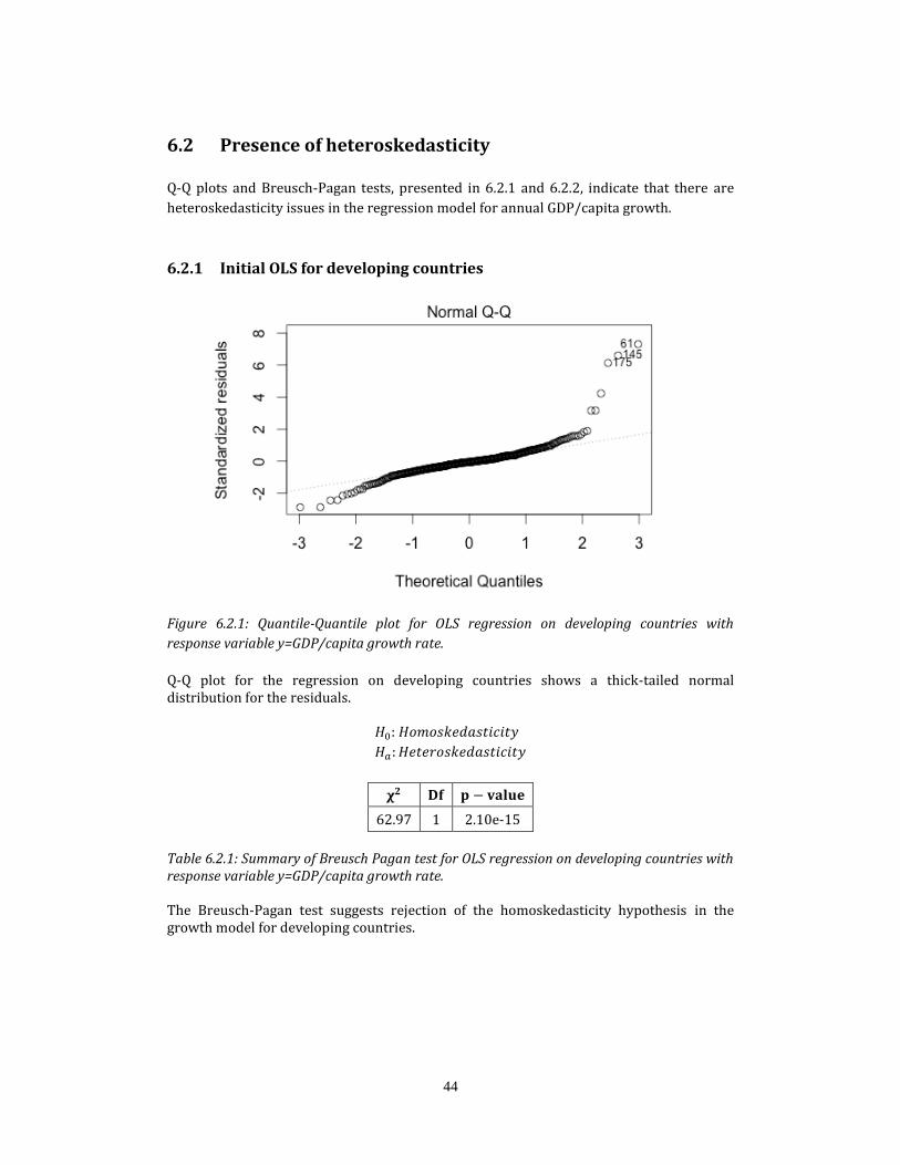
44
6.2 Presence of heteroskedasticity
Q-Q plots and Breusch-Pagan tests, presented in 6.2.1 and 6.2.2, indicate that there are
heteroskedasticity issues in the regression model for annual GDP/capita growth.
6.2.1 Initial OLS for developing countries
Figure 6.2.1: Quantile-Quantile plot for OLS regression on developing countries with
response variable y=GDP/capita growth rate.
Q-Q plot for the regression on developing countries shows a thick-tailed normal distribution for the residuals.
𝐻0: 𝐻𝑜𝑚𝑜𝑠𝑘𝑒𝑑𝑎𝑠𝑡𝑖𝑐𝑖𝑡𝑦
𝐻𝑎: 𝐻𝑒𝑡𝑒𝑟𝑜𝑠𝑘𝑒𝑑𝑎𝑠𝑡𝑖𝑐𝑖𝑡𝑦
𝛘𝟐 𝐃𝐟 𝐩 − 𝐯𝐚𝐥𝐮𝐞
62.97 1 2.10e-15
Table 6.2.1: Summary of Breusch Pagan test for OLS regression on developing countries with response variable y=GDP/capita growth rate. The Breusch-Pagan test suggests rejection of the homoskedasticity hypothesis in the growth model for developing countries.

45
6.2.2 Initial OLS for developed countries
Figure 6.2.2: Quantile-Quantile plot for OLS regression on developed countries with response variable y=GDP/capita growth rate.
Q-Q plot for the regression on developed countries shows a thick-tailed normal
distribution for the residuals.
𝐻0: 𝐻𝑜𝑚𝑜𝑠𝑘𝑒𝑑𝑎𝑠𝑡𝑖𝑐𝑖𝑡𝑦
𝐻𝑎: 𝐻𝑒𝑡𝑒𝑟𝑜𝑠𝑘𝑒𝑑𝑎𝑠𝑡𝑖𝑐𝑖𝑡𝑦
𝛘𝟐 𝐃𝐟 𝐩 − 𝐯𝐚𝐥𝐮𝐞
21.10 1 4.35-06
Table 6.2.2: Table of Breusch-Pagan test for OLS regression on developed countries with
response variable y=GDP/capita growth rate.
As with developing countries, the Breusch-Pagan test suggests rejection of the
homoskedasticity hypothesis in the growth model for developed countries.

46
6.3 Initial robust regression
Instead of OLS, robust regressions are run in order to get more reliable results, presented
in sections 6.3.1 and 6.3.2.
6.3.1 Developing countries
Estimate Std. Error t value Pr(>|t|) Significance level
(Intercept) 3.82005 0.15430 24.757 < 2e-16 ***
GDPi -1.02553 0.18834 -5.445 9.94e-08 ***
Popg -1.25529 0.23815 -5.271 2.42e-07 ***
Ecfree -0.27768 0.17548 -1.582 0.11449
GDI 1.08435 0.17030 6.367 6.24e-10 ***
Educ 0.40107 0.20247 1.981 0.04841 *
FDI 1.13422 0.23923 4.741 3.13e-06 ***
Lifexp 0.07979 0.18563 0.430 0.66760
2009 0.01968 0.53370 0.037 0.97061
2010 -1.53497 0.56197 -2.731 0.00664 **
Significance codes: ‘***’ 0.001, ‘**’ 0.01, ‘*’ 0.05, ‘.’ 0.1.
𝐌𝐮𝐥. 𝐑𝟐 RSE DF
0.3439 1.575 340
Table 6.3.1: Summary of the robust regression for developing countries with y=GDP/capita
growth rate.
Results show no significance for the correlations between GDP/capita growth and Ecfree,
GDI, Lifexp and 2009. All correlations for significant covariates align with what was
expected beforehand in 4.4.3.
6.3.2 Developed countries
Estimate Std. Error t value Pr(>|t|) Significance level
(Intercept) 2.04724 0.11683 17.523 < 2e-16 ***
GDPi -0.02036 0.14978 -0.136 0.8920
Popg -0.23220 0.13124 -1.769 0.0777 .
Ecfree -0.12576 0.14251 -0.882 0.3781
GDI 0.53414 0.12588 4.243 2.85e-05 ***
Educ 0.29338 0.12118 2.421 0.0160 *
FDI 0.72510 0.12299 5.896 9.02e-09 ***
Lifexp -0.81320 0.14936 -5.445 9.98e-08 ***

47
2009 -1.74665 0.42625 -4.098 5.23e-05 ***
2010 -5.62413 0.49400 -11.385 < 2e-16 ***
Significance codes: ‘***’ 0.001, ‘**’ 0.01, ‘*’ 0.05, ‘.’ 0.1.
𝐌𝐮𝐥. 𝐑𝟐 RSE DF
0.3112 2.064 340
Table 6.3.2: Summary of the robust regression for developed countries with y=GDP/capita
growth rate.
Results show no significance for economic freedom and initial level of GDP/capita.
Population growth and education are significant on a 10% and 5% level, respectively. All
significant covariates have the same coefficient signs as expected in 4.4.3.
6.4 Final robust regression
Results from final regressions on both samples are presented in sections 6.4.1 and 6.4.2.
6.4.1 Developing countries
Estimate Std. Error t value Pr(>|t|) Significance level
(Intercept) 5.157358 0.248555 20.749 < 2e-16 ***
GDPi -0.001478 0.000218 -6.779 5.29e-11 ***
Popg -1.289489 0.207666 -6.209 1.54e-09 ***
GDI 1.171815 0.165124 7.097 7.38e-12 ***
Educ 0.373198 0.202101 1.847 0.06567 .
FDI 1.056547 0.228304 4.628 5.25e-06 ***
2010 -1.526813 0.563174 -2.711 0.00704 **
Significance codes: ‘***’ 0.001, ‘**’ 0.01, ‘*’ 0.05, ‘.’ 0.1.
𝐌𝐮𝐥. 𝐑𝟐 RSE DF
0.3061 2.054 343
Table 6.4.1: Summary of the robust regression for developing countries with y=GDP/capita
growth rate.
The final model for developing countries has its coefficient estimates aligning with the
expectations in 4.4.3. All covariates but two are significant on a 0.1% level. Education and
2010 are significant on a 10% and 1% level, respectively.
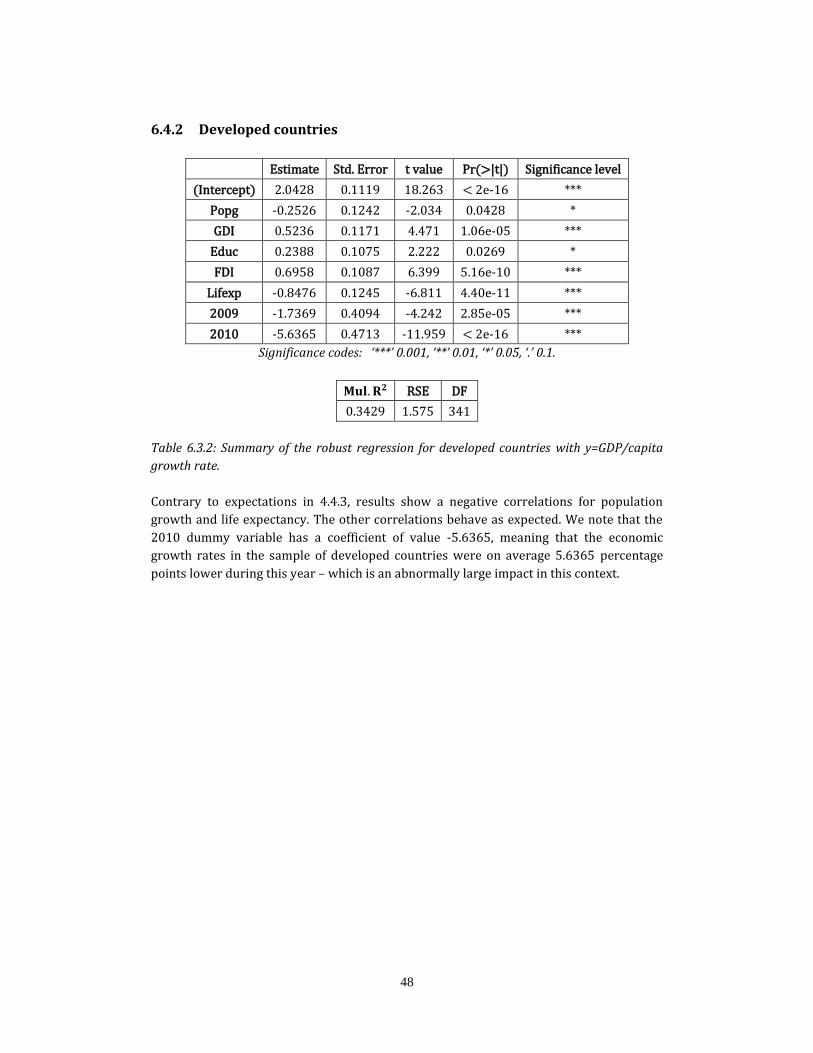
48
6.4.2 Developed countries
Estimate Std. Error t value Pr(>|t|) Significance level
(Intercept) 2.0428 0.1119 18.263 < 2e-16 ***
Popg -0.2526 0.1242 -2.034 0.0428 *
GDI 0.5236 0.1171 4.471 1.06e-05 ***
Educ 0.2388 0.1075 2.222 0.0269 *
FDI 0.6958 0.1087 6.399 5.16e-10 ***
Lifexp -0.8476 0.1245 -6.811 4.40e-11 ***
2009 -1.7369 0.4094 -4.242 2.85e-05 ***
2010 -5.6365 0.4713 -11.959 < 2e-16 ***
Significance codes: ‘***’ 0.001, ‘**’ 0.01, ‘*’ 0.05, ‘.’ 0.1.
𝐌𝐮𝐥. 𝐑𝟐 RSE DF
0.3429 1.575 341
Table 6.3.2: Summary of the robust regression for developed countries with y=GDP/capita
growth rate.
Contrary to expectations in 4.4.3, results show a negative correlations for population
growth and life expectancy. The other correlations behave as expected. We note that the
2010 dummy variable has a coefficient of value -5.6365, meaning that the economic
growth rates in the sample of developed countries were on average 5.6365 percentage
points lower during this year – which is an abnormally large impact in this context.

49
6.5 Economic freedom and economic growth rate
6.5.1 Developing countries
Figure 6.5.1: Simple regression of developing countries on GDP/capita growth rate and Index
of Economic freedom.
As shown by the regressions, there appears to be no clear correlation between economic
freedom and GDP/capita growth for developing countries.
6.5.2 Developed countries
Figure 6.5.2: Simple regression of developed countries on GDP/capita growth rate and Index
of Economic freedom.
Index of Economic Freedom (scaled)
GD
P/
cap
ita
gro
wth
ra
te
Index of Economic Freedom (scaled)
GD
P/
cap
ita
gro
wth
ra
te

50
As for developing countries, no conclusions regarding the effects from economic freedom
on economic growth rate can be drawn for developed countries.
6.6 The convergence hypothesis of the non-extended Solow-
Swan model
Estimate Std. Error t value Pr(>|t|) Significance level
(Intercept) 2.7287 0.1308 20.862 < 2e-16 ***
GDPi -1.2400 0.1474 -8.414 2.25e-16 ***
Popg -0.2757 0.1450 -1.901 0.0577 .
GDI 0.9541 0.1409 6.774 2.68e-11 ***
FDI 0.8802 0.1363 6.457 2.00e-10 ***
Significance codes: ‘***’ 0.001, ‘**’ 0.01, ‘*’ 0.05, ‘.’ 0.1.
𝐀𝐝𝐣. 𝐑𝟐 RSE DF
0.2397 3.458 645
Table 6.6: Summary of the OLS regression for all 50 countries with response variable
Y=GDP/capita growth rate.
In accordance with the convergence hypothesis stated by the non-extended Solow-Swan
model the results indicate that the economic growth rate is higher for countries with a
lower starting level of GDP. Both Gross Domestic Investments and Foreign Direct
Investments are also highly significant and positive, as predicted by the Solow-Swan
model. The convergence theory is not the main focus of this paper (and will therefore not
be further investigated) but nonetheless interesting in this context.

51
7 Discussion
In the following chapter we evaluate the results from chapter 5 and 6. The main focus is
on explaining the results which were unexpected and not predicted by the
macroeconomic theory in chapter 2 and the stated expectations made in the methodology
section. The results are discussed from both economical and mathematical perspectives.
7.1 Result analysis – evaluation of the estimated coefficients
7.1.1 Accounting for endogeneity – are the results reliable?
While the Solow-Swan model is an exogenous growth model, there are reasons to suggest
that some variables may in fact be endogenous from simultaneity - particularly for the
economic output model. For example, wealthier countries afford better education and
may therefore invest in it, which in turn leads to more educated labor force. A more
effective labor force produces more output. At the same time, the level of education affects
the economic output positively on its own. This phenomenon is best described as
simultaneity and is most likely present in more than one covariate. The presence of
simultaneity is taken into consideration throughout the result analysis.
We assume that measurement errors are present in all covariates and response variables.
The data that is used either come from or is based on information from institutions of the
country in question. Given this fact, there is reason to suggest that the accuracy of the
measurements cannot be guaranteed. The measurement errors are likely to have
contributed to endogeneity in the regression models.
Furthermore, omitted variables may have caused biases on the estimates. There are lots of
variables that drive economic growth and output – trying to include as many as possible is
both impractical and increases the risk of multicollinearity and heteroskedasticity.
Ultimately the selection of the final model becomes a tradeoff between complexity and
accuracy of the estimates.

52
7.1.2 Economic output
Developing Developed
Outcome Expected Actual Expected Actual
GDI + + + E
FDI + - + -
Popg - E - +
Educ + + + +
Lifexp + + + +
Ecfree + + + +
Table 7.1.2: Summary of expected outcomes for the coefficients stated in the methodology
section and the actual outcomes for coefficient estimates from the final regression model for
economic output. The letter E indicates that the covariate has been excluded from the final
model.
We note that the expectations for the estimated coefficients were accurate for all
covariates except for Gross Domestic Investments (GDI), Foreign Direct Investments (FDI)
and Population Growth (Popg). This suggests that the Solow-Swan model and its later
extensions can partially explain differences in economic output for the two sample groups.
The unexpected results can be explained through the Solow-Swan convergence theory,
endogeneity and through external empirical findings in economic research.
Surprisingly, population growth was found to be insignificant for developing countries
and positively significant for developed countries. If ceteris paribus is assumed, then
population growth should be negatively correlated with GDP/capita. That is, if population
growth was truly independent and exogenous then the only implication that can be
derived from a higher population growth is that more people get to share the same
amount of economic output, i.e. GDP/capita decreases. However, we suspect that an
inflated standard error (as shown by the VIF test) may have contributed to the
unexpected results for the coefficients of population growth.
A population can grow in different ways demographically and may therefore affect the
economy both positively and negatively. Population growth coming from an increase in
child population will increase the country’s dependency burden and thus hinder short-
term economic development, while population growth consisting of an increase in adults,
i.e. people immigrating, will increase the workforce and thus boost short-term growth
(Crenshaw et al., 1997). Over the observed period (2000-2013), many of the developed
countries have had their population growths largely coming from immigration. In 2009,
59% of the population growth in the EU-28 countries came from net migration (Eurostat,
2014). While this may seem plausible for explaining the unexpected positive correlation

53
between population growth and GDP/capita level in the developed sample group, this is
not supported by our regressions on annual GDP/capita growth rates.
Figure 7.1.2.1: Sources of population growth in EU-28 countries over years 1980-2012.
Source: Eurostat (2014).
The long-term demographic and economic effects from different types of population
growth are complex and will require a thesis on its own to fully elaborate. A widely cited
paper by Simon Kuznets (1960) recognizes that population growth is positively correlated
with per capita output levels for more technologically advanced economies, which is
aligned with our results.
Furthermore, we suspect that the population growth covariate may be endogenous from
simultaneity since richer countries may attract more immigrants - therefore a high
population growth may be indicative of a high economic output. In other words, economic
output affects population growth and vice versa.
GDI was found to be insignificant for developed countries but significantly positively
correlated for developing countries. We believe that this can be partially explained by the
convergence hypothesis stated by Solow-Swan and partially by underestimation bias from
simultaneity. The Solow-Swan model suggests that growth in capital stock (which comes
from investments) has a decreasing marginal yield, which in turn implies that developing
countries have more to gain from gross domestic investments. As seen in figure 7.1.1 the
overall trend among OECD countries is that gross capital formation (which is equivalent to
GDI in our model) as share of GDP has decreased over the last 50 years. However,
decreasing marginal yields must not implicate that the GDI is insignificant. Considering
the Solow-Swan convergence hypothesis, one can argue that a low level of GDI within a
sample group of developed countries indicates a higher GDP/capita level - which in turn
implicates that there could be an underestimation bias for GDI that have contributed to its
insignificance.

54
Figure 7.1.2.2: Gross fixed capital formation as % of GDP for OECD countries and all
countries 1960-2014.
As for GDI, high levels of foreign direct investment is indicative for countries with lower
economic output. This is a reverse causality: rather than FDI having a negative impact on
economic output, it is more likely that low economic output incentivizes large foreign
investments. Furthermore, the negative coefficient for FDI is in accordance with the
convergence theory stated by Solow-Swan, which says that the return of investments are
higher in poorer countries (Barro & Sala-i-Martin, 1995).
Both education and life expectancy were found to be of greater importance among
developing countries, but were nonetheless positive and highly significant for both sample
groups. Our results indicate that increases in human capital levels results in a higher
marginal yield in output for developing countries. These results are in accordance with
the Mankiw-Romer-Weil extension to the Solow-Swan growth model; human capital level
can explain differences in the efficiency of the labor force and are therefore ultimately
important to the economic output (Barro & Sala-i-Martin, 1995).
Economic freedom was found to be highly significant and positively correlated with
economic freedom for both sample groups; these results will be further discussed in
chapter 7.2.
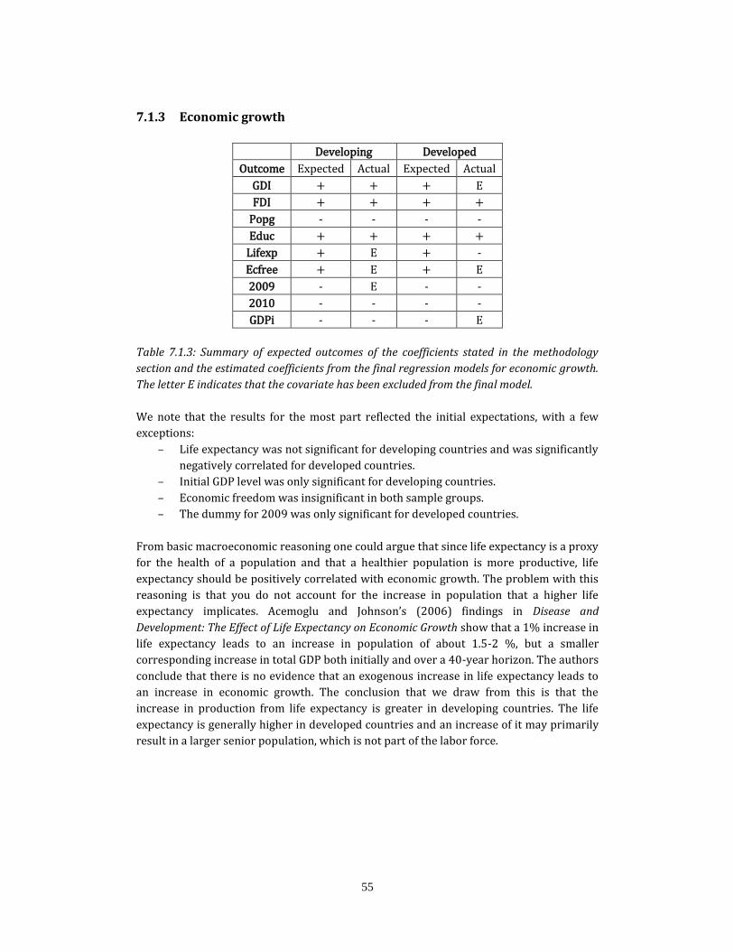
55
7.1.3 Economic growth
Developing Developed
Outcome Expected Actual Expected Actual
GDI + + + E
FDI + + + +
Popg - - - -
Educ + + + +
Lifexp + E + -
Ecfree + E + E
2009 - E - -
2010 - - - -
GDPi - - - E
Table 7.1.3: Summary of expected outcomes of the coefficients stated in the methodology
section and the estimated coefficients from the final regression models for economic growth.
The letter E indicates that the covariate has been excluded from the final model.
We note that the results for the most part reflected the initial expectations, with a few
exceptions:
– Life expectancy was not significant for developing countries and was significantly
negatively correlated for developed countries.
– Initial GDP level was only significant for developing countries.
– Economic freedom was insignificant in both sample groups.
– The dummy for 2009 was only significant for developed countries.
From basic macroeconomic reasoning one could argue that since life expectancy is a proxy
for the health of a population and that a healthier population is more productive, life
expectancy should be positively correlated with economic growth. The problem with this
reasoning is that you do not account for the increase in population that a higher life
expectancy implicates. Acemoglu and Johnson’s (2006) findings in Disease and
Development: The Effect of Life Expectancy on Economic Growth show that a 1% increase in
life expectancy leads to an increase in population of about 1.5-2 %, but a smaller
corresponding increase in total GDP both initially and over a 40-year horizon. The authors
conclude that there is no evidence that an exogenous increase in life expectancy leads to
an increase in economic growth. The conclusion that we draw from this is that the
increase in production from life expectancy is greater in developing countries. The life
expectancy is generally higher in developed countries and an increase of it may primarily
result in a larger senior population, which is not part of the labor force.

56
Figure 7.1.3.1: Simple regression for developed countries showing a significant negative
correlation between economic growth life and expectancy.
Figure 7.1.3.2: Simple regression for developing countries showing an insignificant
correlation between economic growth and life expectancy.
The insignificance of initial GDP level implies that the Solow-Swan convergence theory
does not hold true for our sample group of developed countries. Results for economic
freedom and the 2009 and 2010 dummies are discussed in the next section.
GD
P/
cap
ita
gro
wth
ra
te
Life expectancy (scaled)
Life expectancy (scaled)
GD
P/
cap
ita
gro
wth
ra
te

57
7.2 What are the effects on GDP/capita level and GDP/capita
growth from economic freedom among developing and
developed countries?
As seen in chapter 5, there is a significant positive correlation between economic freedom
and economic output for both sample groups. This correlation implies that countries with
a high economic output to a higher degree fulfill the requirements for achieving a high
score in the Heritage foundation’s Index of Economic Freedom. It is noted that the
correlation is somewhat stronger in developed countries than among developed
countries, which implies that wealthier countries have a bigger marginal gain from raising
their level of Economic freedom in terms of economic output.
We cannot fully reject that there is a reversed causal relationship between economic
output and economic freedom – i.e. that wealthier countries can “afford” more economic
freedom. But the correlation is strongly positive within both sample groups, which
suggests that economic freedom is not a luxury good only for the richest countries. Our
results indicate that the level of economic freedom is important in describing relative
differences in economic output within the sample groups. Furthermore, results found by
Heckelman (2000) on the causality between economic freedom and economic growth
favors a non-reverse causality relationship. Combined with our own results, this
strengthens the hypothesis that economic freedom is important for economic output and
ultimately long-term economic growth.
In the robust regressions in chapter 6, the level of economic freedom showed no
significant correlation with economic growth. The results indicate that economic freedom
cannot be regarded as a driver for economic growth during the period 2000-2013.
However, we do acknowledge that the economic growth during the period 2009-2013 has
been abnormal as a result of the financial crisis and may very well not reflect results from
previous decades.
Judging from the sizes of the coefficients for dummies 2009 and 2010, the financial crisis
had the greatest negative impact, in terms of economic growth rate, on the developed
countries. Furthermore, we note that there is a lag in the effects on developing countries
from the financial crisis, where 2009 was insignificant for developing countries but
strongly negatively correlated and significant for developed countries. This is most
probably due to a lower degree of integration in the global financial system, which
isolated many developing countries from direct economic impact (AFDB, 2009).
The link between the recent financial crisis and economic freedom has been subject to
debate and research, without any definite conclusions. More specifically, some argue that
deregulation of the financial system (primarily in the USA) was the source of the subprime
mortgage- and banking crisis of 2008 (e.g. Crotty, 2009). Some even argue that capitalism
is inherent to financial crises (Buiter, 2007). On the contrary, countries with a high degree
of economic freedom have been shown to recover faster from financial crises than
58
countries with a low degree of freedom (De Haan et al., 2007) and that economic freedom
in fact reduces the risk of financial crises (Björnskov, 2015).
It is true that developed countries generally score higher in the Index of Economic
Freedom; on average, our sample group of developed countries scores 71.91/100, while
the developing countries score 56.05/100. It is also true that the financial crisis had
greater negative impact on economic growth among developed countries – but this does
not entail any causal relationship between the financial crisis and economic freedom. Our
results tell us that the level of economic freedom has been insignificant to economic
growth over the period 2000-2013 - we choose not to draw any further conclusions on
this issue.
7.4 Concluding remarks
From the results and the discussion we draw the following conclusions:
Wealthier countries tend to have a higher level of economic freedom, both among
developing and developed countries.
The level of economic freedom is insignificant for economic growth in both of our
sample groups of developed and developing countries for years 2000-2013.
Our results indicate that improvements in education, gross domestic investments
and foreign direct investments produce a higher marginal yield in economic
growth for developing countries.
Our results indicate that the initial level of GDP is insignificant to the economic
growth rate for a sample group of developed countries.
The financial crisis in 2008 had a greater impact on our sample group of
developed countries in terms of economic growth, compared to the sample group
of developing countries.
7.5 Suggestions for further research We have recognized the need for further research on the topic of economic growth and
economic freedom. We hope to see the following from future research:
An examination on the relationship between economic freedom and the recent
financial crisis. While a case study has been conducted by De Haan et al. (2009)
on Sweden and Norway, we see a need for a larger sample group and a more
general conclusion.
More nuanced sample group divisions containing for example emerging
economies, sample groups based on human development indices (HDI) and
economic freedom indices.

59
An empirical examination on how economic freedom correlates with the
frequency and magnitude of business cycle fluctuations. Does the lack of
regulations make the economy more volatile?
60
8 References Acemoglu D, Johnson S, 2006, “Disease and Development: The Effect of Life Expectancy on Economic Growth”, NBER Working Paper series, No.12269, National Bureau of Economic Research (June 2006). Barro R, 1991, “Economic Growth in a Cross Section of Countries”, The Quarterly Journal of Economics, Vol. 106, No. 2. (May 1991). Barro R, Lee J.W, 1994, “Sources on Economic Growth”, Carnegie-Rochester Conference Series on Public Policy, Vol. 40 (June 1994), incorporated in Journal of Monetary Economics. Barro R, Lee J.W, 2013 “A new set of educational attainment in the world, 1950-2010”, Journal of Development Economics, Vol. 104 (Sep. 2013) Barro R, Sala-i-Martin X, 1995, Economic growth, 2nd edition, The MIT Press. Bjørnskov C, 2015, “Economic Freedom and Economic Crisis”, IFN Working Paper, No. 1056, Research Institute of Industrial Economics (Jan. 2015). Buiter W.H, 2007, “Lessons from the 2007 Financial Crisis”, CEPR Discussion Paper No.
6596, Center for Economic Policy Research (Dec. 2007).
Carroll R.J, Ruppert D, 1998, Transformation and Weighting in Regression, Chapman & Hall, 1998. Cass D, 1965, “Optimum Growth in an Aggregate Model of Capital Accumulation”, Review of Economic Studies, Vol. 32, No. 3 (July 1965). Crotty J, 2009, “Structural causes of the global financial crisis: a critical assessment of the ‘new financial architecture’”, Cambridge Journal of Economics, Vol. 33 (May 2009). De Haan J, Sturm J-E, 1999, “On the relationship between economic freedom and economic growth”, European Journal of Political Economy, Vol. 16 (2000). De Haan J, Sturm J-E, Zandberg E, 2009, “The Impact of Financial and Economic Crises on Economic Freedom”, Economic Freedom of the World: 2009 Annual Report (2009). Eaton J, Kortum S, 1995, “Engines of growth: Domestic and Foreign Sources of Innovation”, Japan and the World Economy, Vol. 9, issue 2 (Nov. 1997). Gwartney J, Lawson R, Norton S, “Economic freedom and the environment for economic growth”, Journal of Institutional and Theoretical Economics, Vol. 155, No. 4 (Dec. 1999). Hall R.E, Jones C.I, 1996, “The Productivity of Nations”, NBER Working Paper Series, No. 5812, National Bureau of Economic Research (Nov. 1996). Hall R.E, Jones C.I., 1998, “Why do Some Countries Produce So Much More Output per Worker than Others?”, Quarterly Journal of Economics, Vol. 114 (Feb., 1999).

61
Hansen B, 2000, Econometrics, 2014 edition, University Of Wisconsin. Heckelman J.C, 2000, “Which Economic Freedoms Contribute to Growth?”, Kyklos, Vol. 53 (Nov. 2000). Heij C, de Boer P, 2004, Econometric Methods with Applications in Business and Economics, 1st edition, Oxford University Press. Jacoby B, 2005, “Regression III: Advanced Methods”, workshop notes distributed in 2005 ICPSR Summer Training Program in Quantitative Methods of Social Research at Michigan State University on July 14th 2005. Kremer M, Pritchett L, Summers L.H, Easterly W, 1993, “Good policy or good luck? Country growth performance and temporary shocks”, Journal of Monetary Economics, Vol. 32 (Sep. 1993). Krugman P, Wells R, 2009, Economics, 2nd edition, Worth Publishers. Lang H, 2014, Elements of Regression Analysis, textbook distributed for SF2950 Applied Mathematical Statistics at Royal Institute of Technology, spring 2015. Lütkepohl H, Xu F, 2009, “The Role of Log Transformation in Forecasting Economic Variables”, CESifo working paper series, No.2591, Munich Society for the Promotion of Economic Research (March 2009). Mankiw N.G, Romer D, Weil D.N., 1992, “A Contribution to the Empirics of Economic Growth”, Quarterly Journal of Economics, Vol. 107 (May 1992). North D.C, Thomas R.P, 1973, The Rise of the Western World: A new Economic History, Cambridge University Press (1973). Office of the Chief Economist, African Development Bank, “Impact of the Global Financial and Economic Crisis on Africa” (Feb. 2009). Parente S, Prescott E, 1994, ”Barriers to Technology Adoption and Development”, Journal of Political Economy, Vol. 102 (Apr. 1994). Scully G.W, Slottje D.J, 1991, “Ranking Economic Liberty across Countries”, Public Choice, Vol. 69, No. 2 (Feb., 1991). Solow R, 1956, ”A Contribution to the Theory of Economic Growth”, The Quarterly Journal of Economics, Vol 70, No. 1 (Feb. 1956). Studenmund A.H, 2006, Using Econometrics: A practical Guide, 6th edition, Pearson International. Swan, T, 1956, “Economic Growth and Capital Accumulation”, Economic Record, Vol. 32 (Nov. 1956). Torstensson J, 1994, “Property Rights and Economic Growth: An Empirical Study”, Kyklos, Vol. 47 (May 1994).
62
Vanssay, X, Spindler, Z.A, 1994, “Freedom and growth: Do constitutions matter?”, Public Choice, Vol. 78 (March 1994).
8.1 Data sources
8.1.1 Data used in regression
Heritage Foundation 2015, Index of Economic Freedom. Available from www.heritage.org/index/about. Barro-Lee dataset on educational attainment. Available from http://www.barrolee.com/data/yrsch2.htm. World Bank database. Available from http://data.worldbank.org/.
8.1.2 Miscellaneous EuroStat data on causes of population growth in the EU. Available from http://ec.europa.eu/eurostat/data/database.

63
A Appendix
A1 Samples of developing and developed countries
Developed Countries Developing Countries
Australia Algeria
Austria Azerbaijan
Canada Bangladesh
Croatia Belarus
Czech Republic Benin
Denmark Bolivia
Estonia Botswana
Finland Cambodia
France Cameroon
Germany Chad
Hong Kong China
Iceland Ecuador
Ireland Egypt
Israel El Salvador
Italy Ethiopia
Japan Georgia
New Zealand Ghana
Norway Guatemala
Poland Guinea
Portugal India
Spain Indonesia
Sweden Kenya
Switzerland Morocco
United Kingdom Nigeria
United States Tanzania
64
A2 Motivations for initial expectations of coefficient estimate
outcomes
Gross Domestic Investment (GDI)
Increased investments increases the capital stock; GDI is therefore expected to be
positively correlated with both economic output and economic growth.
Foreign Direct Investment (FDI)
Increased investments increases the capital stock; FDI is therefore expected to be
positively correlated with both economic output and economic growth.
Population growth (Popg)
Increased population means that the denominator is increased in the GDP/capita and
GDP/capita growth measures. Population growth is therefore expected to be negatively
correlated with economic output and economic growth.
Education (Educ)
Increased education increases human capital, resulting in increased productivity.
Education is therefore expected to be positively correlated with economic output and
economic growth.
Life expectancy (Lifexp)
Life expectancy is seen as a proxy on the overall population health and the quality of the
country’s healthcare system. A healthy population is assumed to be more productive; life
expectancy is therefore expected to be positively correlated with economic output and
economic growth.
Economic freedom (Ecfree)
A favorable social infrastructure is assumed to be aligned with a high degree of economic
freedom. Economic freedom is therefore expected to be positively correlated with
economic output and economic growth.
Initial level of GDP/capita (GDPi)
According to the non-extended Solow model, countries will over time experience a
convergence in economic progress: poorer countries are expected to outgrow richer
countries. Initial level of GDP/capita is therefore expected to have a negative correlation
with economic growth.

65
Dummies: 2009 and 2010
Following the start of the financial crisis in 2008, dummies for 2009 and 2010 are
introduced to increase the explanatory value of the growth regression model. Both
dummies are expected to be negatively correlated with economic growth.


TRITA -MAT-K 2015:10
ISRN -KTH/MAT/K--15/10--SE
www.kth.se