modeling bus load on can - diva portal540300/fulltext01.pdf · 1- starting application ......
TRANSCRIPT

Master report, IDE 1250, July 2012
Modeling Bus Load on CAN
Mas
ter t
hesi
s Sc
hool
of I
nfor
mat
ion
Scie
nce,
Com
pute
r and
Ele
ctric
al E
ngin
eerin
g
Musab Al Hayani

Modeling Bus Load on CAN
Master Thesis
Embedded and Intelligent Systems Master Program
School of Information Science, Computer and Electrical Engineering
Halmstad University
July 2012
Musab Al Hayani School of Information Science, Computer and Electrical Engineering
Halmstad University The Author
Jan Lindman System Architecture (RESA)
Research and Development, Scania AB The Supervisor
Tony Larsson Professor of Embedded Systems
Halmstad University The Examiner
School of Information Science, Computer and Electrical Engineering Halmstad University
PO Box 823, SE-301 18 HALMSTAD, Sweden
I
Modeling Bus Load on CAN Musab Al Hayani
Copyright MUSAB AL HAYANI, 2012. All rights reserved. Master Thesis
Report, IDE1250
School of Information Science, Computer and Electrical Engineering
Halmstad University
ISSN
This work has been fully sponsored by:
System Architecture (RESA),
Research and Development, Scania Technical Center, Scania AB
Södertälje, Sweden
Telephone +46 (0)8-553 89411

II
Preface
This titled master thesis has been done at the Research and Development/System Architecture Dept. in Scania Technical Center, Södertälje, Sweden as a result of my studies at Halmstad University, Halmstad, Sweden.
I take this opportunity to thank several people who gave me their support during my Thesis preparation days at Södertälje and during my Post graduation at Halmstad.
Deep and special thanks go first to Jan Lindman, my supervisor at Scania, for his intensive comments, instructions, guidance, testing and tracking.
To Prof. Tony Larsson, my supervisor and examiner at Halmstad University for his patience and unlimited explanations, valuable instructions and support.
To David Holmgren, the RESA Group Manager for his instructions and comments.
To my father, mother and wife, I have received intensive and unlimited support from them.
Musab Al Hayani
Södertälje, 7th of July 2012

III
Abstract
The existence of high load and latency in the CAN bus network would indeed lead to a situation where a given message crosses its deadline; this situation would disturb the continuity of the required service as well as activating fault codes due to delay of message delivery, which might lead to system failure.
The outcome and goal of this thesis is to research and formulate methods to determine and model busload and latencies, by determining parameters such as alpha and breakdown utilization, which are considered as indications to the start of network breakdown when a given message in a dataset start to introduce latency by crossing its deadline which are totally prohibited in critical real time communications.
The final goal of this master thesis is to develop a TOOL for calculating, modeling, determining and visualizing worst case busload, throughput, networks’ breakdown points and worst case latency in Scania CAN bus networks which is based on the J1939 protocol.
SCANLA (The developed CAN busload analyzer tool in this thesis) is running as an executable application and uses a Graphical User Interface as a human-computer interface (i.e., a way for humans to interact with the tool) that uses windows, icons and menus and which can be manipulated by a mouse.
The CAN Tool consists of: CAN_TOOL.fig (The Human-Tool Interface), CAN_TOOL.m, CAN_App.m, mydatabase.m, Plotting.m, BreakDown.m, ResponseTime.m, logfiles, associated databases and accompanying documents, such as this thesis report. This Tool is hoped that it will be useful but without any warranty.
For a description and instructions on how to use the tool, read intensively the report.
Please let the producer of the mentioned tool know of any improvements, changes or modifications that might be made.
Musab Al Hayani. [email protected]
Thesis Supervisor: Jan Lindman
Title: Modeling Bus Load on CAN

IV
Table of Contents PREFACE ............................................................................................................................................................ II
ABSTRACT ......................................................................................................................................................... III
TABLE OF CONTENTS .................................................................................................................................... IV
LIST OF TABLES ................................................................................................................................................ V
TABLE OF FIGURES ........................................................................................................................................ VI
TERMS & DEFINITIONS ............................................................................................................................... VII
CHAPTER 1. INTRODUCTION .................................................................................................................. 1
1.1 PROBLEM STATEMENT ........................................................................................................................... 1 1.2 APPROACH SOLUTION TO THE PROBLEM ................................................................................................ 2 1.3 THESIS GOALS AND EXPECTED RESULTS ............................................................................................... 3 1.4 PROGRAMMING TOOL ENVIRONMENT .................................................................................................... 4
CHAPTER 2. BACKGROUND ..................................................................................................................... 5
2.1 WHY CONTINUE TO RELY ON ‘CAN’ ...................................................................................................... 6 2.2 SCANIA CAN BUS APPLICATION ............................................................................................................ 7 2.3 APPLIED J1939 PROTOCOL ON SCANIA CAN BUS NETWORKS ................................................................ 8 2.4 BUS NETWORK LENGTH .......................................................................................................................... 9 2.5 J1939 SPECIFICATIONS: .......................................................................................................................... 9
2.5.1 Message Format of J1939-21 ..................................................................................................... 10 2.5.2 Translation of PF and PS contents ............................................................................................. 11 2.5.3 1939-21 CAN Messages Arbitration ........................................................................................... 12
2.6 STATE OF THE ART ............................................................................................................................... 13 2.7 CLOSELY RELATED WORK ................................................................................................................... 14
CHAPTER 3. LOAD ANALYSIS MODEL ............................................................................................... 15
3.1 ASSUMPTION OF MESSAGES’ ARRIVAL TIME ........................................................................................ 15 3.2 CALCULATION OF MESSAGE TRANSMISSION TIME................................................................................. 16 3.3 APPLYING THE SCHEDUABILITY ANALYSIS .......................................................................................... 16 3.4 CALCULATION OF LATENCY ................................................................................................................. 19 3.5 CALCULATION OF ALPHA & BREAKDOWN UTILIZATION ....................................................................... 20
3.5.1 Introduction ................................................................................................................................ 20 3.5.2 Definition .................................................................................................................................... 20 3.5.3 Translation .................................................................................................................................. 20 3.5.4 Possibilities ................................................................................................................................. 21 3.5.5 Modeling ..................................................................................................................................... 21
3.6 FURTHER BUSLOAD .............................................................................................................................. 21
CHAPTER 4. FLOWCHART OF TOOL FUNCTIONS .......................................................................... 22
CHAPTER 5. GRAPHICAL USER INTERFACE GUI ........................................................................... 23
5.1 THE TOOL’S INPUT ............................................................................................................................... 23 5.2 THE TOOL’S OUTPUT............................................................................................................................ 24

V
CHAPTER 6. TEST RESULTS & ANALYSIS ......................................................................................... 28
6.1 TEST 1, A REALISTIC TEST BASED ON CAN LOG FILE FROM T VEHICLE ................................................ 29 6.1.1 Resulted Breakdown Utilization & alpha ................................................................................... 31 6.1.2 Encountered Latencies ................................................................................................................ 31 6.1.3 Suggested Solution ...................................................................................................................... 31
6.2 RUNNING TEST 2 ON THE REPAIRED YELLOW BUS ................................................................................ 32 6.2.1 Resulted Breakdown Utilization & alpha ................................................................................... 32 6.2.2 Discussion ................................................................................................................................... 32
6.3 REFERENCE TEST ................................................................................................................................. 33 6.3.1 Resulted Breakdown Utilization & alpha ................................................................................... 34 6.3.2 Test Inferences ............................................................................................................................ 34
CHAPTER 7. MODELING OF DIAGNOSTIC LOAD ............................................................................ 35
7.1 MODELING OF KWP2000 DIAGNOSTIC MESSAGES LOAD .................................................................... 35 7.2 RESPONSE TIME ANALYSIS WHEN INITIATING WORST CASE SCENARIO, WITH KWP2000 SERVERS ....... 35
7.2.1 Resulted Breakdown Utilization & alpha of diagnostic Test ...................................................... 38 7.2.2 Discussion ................................................................................................................................... 38 7.2.3 Inference ..................................................................................................................................... 39
CHAPTER 8. CONCLUSIONS ................................................................................................................... 40
8.1 SUGGESTIONS TO FUTURE WORK ......................................................................................................... 40
REFERENCES .................................................................................................................................................... 41
APPENDIX A INSTRUCTIONS ON HOW TO USE SCANLA ................................................................. 42
1- STARTING APPLICATION ................................................................................................................... 42
2- GETTING THE INPUT ............................................................................................................................ 42
3- SELECTING THE SIMULATION MODE ............................................................................................ 42
4- RUNNING THE ANALYSIS TOOL ....................................................................................................... 43
5- PRODUCING THE OUTPUT ................................................................................................................. 44
APPENDIX B SCANIA T, CAN TRAFFIC TTR REPORTS ..................................................................... 45
APPENDIX C SCANIA T, CAN RESSPONSE TIME ANALYSIS ............................................................ 48
List of Tables Table 1 CAN bus bit rate / length ......................................................................................................................... 9Table 2 Test1 Resulted Breakdown Utilization & alpha .......................................................................... 31Table 3 Test2 Resulted Breakdown Utilization & alpha .......................................................................... 32Table 4 Ref. Test Resulted Breakdown Utilization & alpha .................................................................... 34Table 5 Ddiagnostic Test, Resulted Breakdown Utilization & alpha .................................................. 38
VI
Table of Equations Equation 1 - - - - Message transmission time ...................................................................................................... 16Equation 2 - - - - Message Waiting time / Relative ............................................................................................ 16Equation 3 - - - - Message Max. Blocking time / Relative ............................................................................. 17Equation 4 - - - - Number of message invoications ........................................................................................... 18Equation 5 - - - - Message Busy Period ................................................................................................................... 18Equation 6 - - - - Message Response time / Relative ........................................................................................ 19Equation 7 - - - - Message worst case response time ........................................................................................ 19Equation 8 - - - - Message Latency time ................................................................................................................. 19
Table of Figures Figure 1 Typical CAN Bus ............................................................................................... 5
Figure 2 Schematic Diagram of Scania CAN Bus Networks ................................................ 8
Figure 3 Standard J1939 network model ......................................................................... 9
Figure 4 Typical Format of J1939-21 Message ................................................................10
Figure 5 CAN Dominant (0) & Recessive (1) in term of Voltage ........................................12
Figure 6 Typical CAN J1939 messages arbitration ...........................................................13
Figure 7 Flowchart of the ‘Mathematical Solution’ to model CAN bus load .......................15
Figure 8 Flowchart of CAN Tool code to model bus load on CAN ......................................22
Figure 9 Snapshot of the Produced Human –CAN_TOOL Interface using of GUI ................25
Figure 10 Sample of the red bus traffic report. ..................................................................26
Figure 11 Sample of the red bus response time analysis ....................................................26
Figure 12 Sample of the different networks’ breakdown point ...........................................27
Figure 13 Sample of a green bus latency/response time plot .............................................27
Figure 14 Response Time (Test1) of Green Bus Messages Invocation 1 ..............................29
Figure 15 Response Time (Test1) of Red Bus Messages Invocation 1 .................................29
Figure 16 Response Time (Test1) of Yellow Bus Messages Invocation 1 .............................30
Figure 17 Response Time (Test1) of Yellow Bus Messages Invocation 2 .............................30
Figure 18 Response Time (Test2) of Yellow Bus Messages Invocation 1 .............................32
Figure 19 Response Time (Ref. Test) of Red Bus Messages Invocation 1 .............................33
Figure 20 Response Time (Ref. Test) of Red Bus Messages Invocation 2 .............................33
Figure 21 Response Time (Diagnostic Test) of Red Bus Messages Invocation 1 ...................36
Figure 22 Response Time (Diagnostic Test) of Green Bus Messages Invocation 1 ...............36
Figure 23 Response Time (Diagnostic Test) of Yellow Bus Messages Invocation 1 ..............37
Figure 24 Response Time (Diagnostic Test) of Yellow Bus Messages Invocation 2 ..............37
VII
TERMS & DEFINITIONS CAN Controller Area Network
ECU Electronic Control Unit
SA Source Address
PG Parameter Group
PGN Parameter Group Number
COO Coordinator to isolate buses & gateway specific messages.
BP Busy Period
Tr Response Time
Td Deadline Time
Tp Cycle Time
Node Group of related functions allocated in one physical ECU
CANalyzer CAN Analyzer tool for testing & visualizing real time bus response time
MATLAB Programming Environment
OSI Open Systems Interconnection model, which gives standard layers for communication functions.
J1939 Heavy vehicle standard for communication over CAN bus.
TTR CAN Traffic Technical Report
Latency Time remaining (which need to be used) to finish a message execution after its deadline
Utilization Percentage of the achieved throughput over baud rate.
Alpha Indication of how much useful slack time there is in the system
Breakdown Utilization Bus breakdown point which happens when bus start to introduce latencies.
Priority in CAN Message Importance value statically given to CAN messages.
Blocking Time Time Delay of Message Execution due to suspension by higher priority message or due to wait for a free resource to use
OBD On Board Diagnostic
DTC Diagnostic Trouble Code
KWP2000 Keyword Diagnostic protocol
GUI Graphical User Interface
SCANLA SCANIA CAN Bus Load Analyzer (The Produced CAN Tool)

Modeling Bus Load on CAN
Page 1
CHAPTER 1. INTRODUCTION
1.1 PROBLEM STATEMENT As the development in automotive industry is growing rapidly, more sensors, CAN signals and CAN messages are added to the vehicle CAN bus networks and therefore more electronic control modules (ECUs) are added to those networks, which means more CAN bus networks are added to the vehicle.
As a result higher load will be introduced and should be calculated and checked to see its impact on CAN messages which could vary from delaying message delivery (latency) or stop delivering of those messages.
To get a better understanding of the nature of those CAN messages in Automation, let us assume the following examples in both hard and soft real time CAN messages; check out the following two examples:
Ex1, if a specific hard real time CAN bus has received a load that drove some messages to cross deadlines; in other words, latency is introduced, such as:
Failing to deliver messages of hard real time nature could lead sometimes to serious consequences such as AirBagSgnMsg hard real time airbag message in example-1 which is considered as a disaster to vehicle industry that could lead to multi hundred million Krona loss as well as loss of lives, while a better case could lead to system failure such as GearBoxTrMsg hard real time gear box change message in example-1.
Ex2, if a specific soft real time CAN bus has received a load that drove some messages to cross deadlines; in other words, latencies are introduced, such as:
Example-1 The results of delayed hard real time messages
Example-2 The results of delayed hard real time messages
Modeling Bus Load on CAN
Page 2
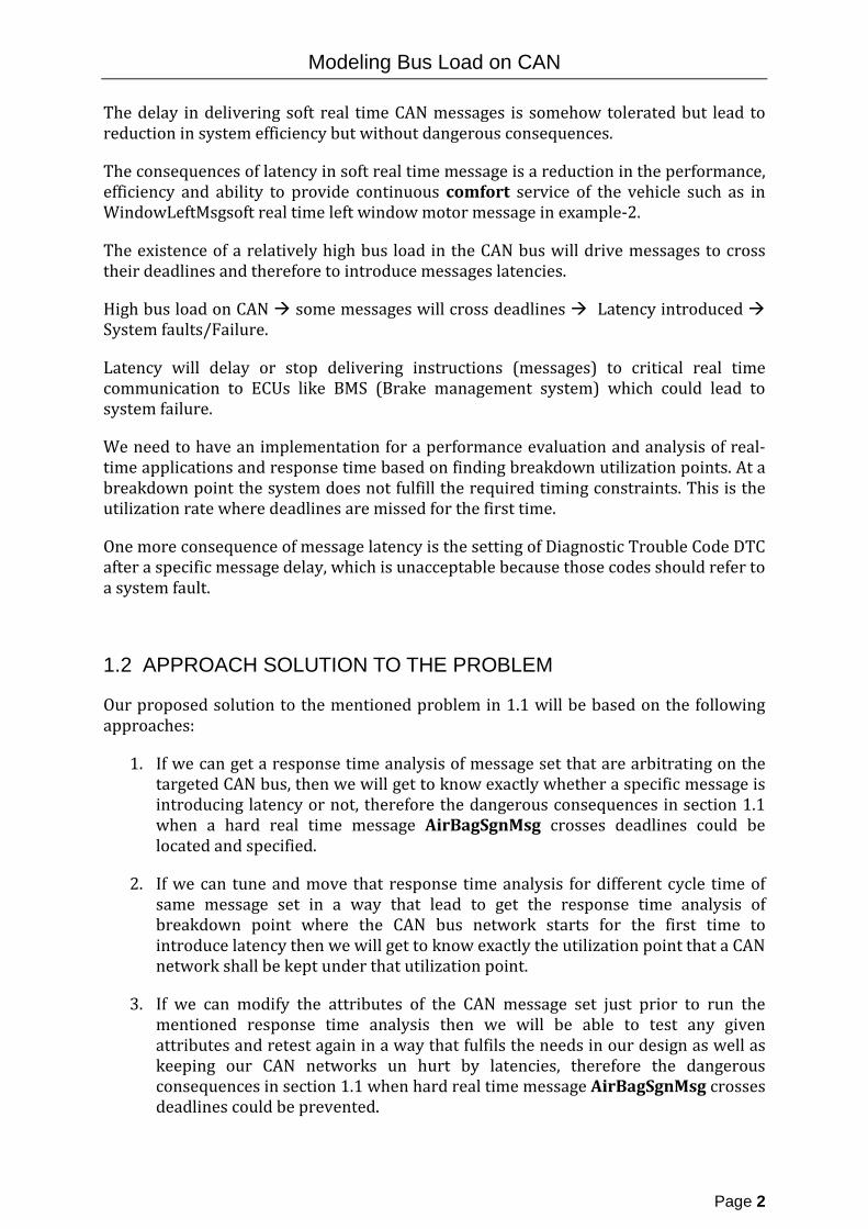
The delay in delivering soft real time CAN messages is somehow tolerated but lead to reduction in system efficiency but without dangerous consequences.
The consequences of latency in soft real time message is a reduction in the performance, efficiency and ability to provide continuous comfort service of the vehicle such as in WindowLeftMsgsoft real time left window motor message in example-2.
The existence of a relatively high bus load in the CAN bus will drive messages to cross their deadlines and therefore to introduce messages latencies.
High bus load on CAN some messages will cross deadlines Latency introduced System faults/Failure.
Latency will delay or stop delivering instructions (messages) to critical real time communication to ECUs like BMS (Brake management system) which could lead to system failure.
We need to have an implementation for a performance evaluation and analysis of real-time applications and response time based on finding breakdown utilization points. At a breakdown point the system does not fulfill the required timing constraints. This is the utilization rate where deadlines are missed for the first time.
One more consequence of message latency is the setting of Diagnostic Trouble Code DTC after a specific message delay, which is unacceptable because those codes should refer to a system fault.
1.2 APPROACH SOLUTION TO THE PROBLEM
Our proposed solution to the mentioned problem in 1.1 will be based on the following approaches:
1. If we can get a response time analysis of message set that are arbitrating on the targeted CAN bus, then we will get to know exactly whether a specific message is introducing latency or not, therefore the dangerous consequences in section 1.1 when a hard real time message AirBagSgnMsg crosses deadlines could be located and specified.
2. If we can tune and move that response time analysis for different cycle time of same message set in a way that lead to get the response time analysis of breakdown point where the CAN bus network starts for the first time to introduce latency then we will get to know exactly the utilization point that a CAN network shall be kept under that utilization point.
3. If we can modify the attributes of the CAN message set just prior to run the mentioned response time analysis then we will be able to test any given attributes and retest again in a way that fulfils the needs in our design as well as keeping our CAN networks un hurt by latencies, therefore the dangerous consequences in section 1.1 when hard real time message AirBagSgnMsg crosses deadlines could be prevented.

Modeling Bus Load on CAN
Page 3
Our targets’ system behavior is:
1- For hard real time CAN signals and messages, preventing system faults and failures of latency causes (that could lead sometimes to disaster to vehicle industry).
2- For soft real time CAN signals and messages, preventing the reduction in the system efficiency which caused by latency in those CAN signals and messages
It is important to keep all CAN messages delivered within their correspondent deadlines to ensure the continuity of the service especially for hard real time CAN messages; therefore I decided to built a tool that can analyze CAN networks to see its load, breakdown load and catching latency if exists.
1.3 THESIS GOALS AND EXPECTED RESULTS
Based on the approach solution proposed in 1.2 and in order to keep all CAN messages delivered within their correspondent deadlines to ensure the continuity of the service especially for hard real time CAN messages; therefore I decided to build a tool that is capable of:
1- Simulating and modeling CAN bus load and message latencies
2- Showing latencies if they exist in the bus network. Most of normally loaded CAN bus networks introduce latencies; while the lightly loaded CAN bus networks of course are free from latencies. Some latencies can be tolerated while the others can’t be tolerated and should be prevented based on the how much critical are the timing behavior of the signals embedded in those late CAN messages).
3- Analyzing of a given bus network to determine response time analysis of all messages under test which will improve our understanding on how a specific CAN bus network behave during different run, still or wake up modes .
4- Showing how much useful free slack time is there in the network
5- Testing a given network to determine by how much it could handle an extra load
The Tool should be able to model and visualize the busload and latencies of Scania CAN buses/messages using multiple combinations of Scania’s (User Functions) Messages, and apply them in their worst case scenario.
We need to have an implementation of real-time applications analysis which is based on finding breakdown utilization points. At a breakdown point the system does not fulfill the required timing constraints. This is the utilization rate where deadlines are missed for the first time. With our implementation we observe the system behind the breakdown utilization; we observe the system behavior under overload conditions.
The ability to visualize latency of each message will intensively help to locate the point in time when a given message or a bunch of messages would cross their deadlines and as a result, visualizing latency would indeed help to overcome the reason behind it.

Modeling Bus Load on CAN
Page 4
Calculation of the Breakdown Utilization will give us a value which indicates how much slack time there is in the network.
One of the main expected results is to determine parameters like ‘breakdown utilization’ and ‘alpha’ which are considered as an indications to the start of network breakdown when a given message in a dataset starts to cross deadline which is not allowed in critical real time communications.
1.4 PROGRAMMING TOOL ENVIRONMENT
I selected MATLAB as a suitable programming environment to model the whole TOOL and to compute data analysis, visualization, and numerical computation. MATLAB resolves technical computing problems faster than traditional programming languages, such as C, FORTRAN, and C++.
MATLAB is widely used in applications like signal and image processing, control design, communications, test and measurement, modeling and analysis, and computational biology.

Modeling Bus Load on CAN
Page 5
CHAPTER 2. BACKGROUND
Controller Area Network (CAN bus network) is a serial communications bus network which is basically designed and manufactured to support simple and robust communications for Bosch’s inVehicle bus networks.
In a regular vehicle, there exists tens of thousands of unique and distinct signals and most of them have the nature of real time and some of them are critical real time, where the CAN bus network have replaced their thousands of point to point wiring methods and integrated them into one to seven bus networks .
The CAN bus network is set among multiple electronics which helps translation and interfaces between multiple systems. Those electronics include CAN gateways, CAN embedded controllers, Hardware interface, and CAN converters.
Heavy duty vehicles did identify the CAN bus (especially the J1939 protocol) as powerful and the most reliable bus network ever used in what is known as (inVehicle communications).
Today every vehicle that is made in USA, Japan, Europe and Korea is equipped with at least two CAN bus networks [1]
In some countries such as the USA, implementing and using of CAN bus network is obligatory.
The above figure shows a typical CAN bus topology, here I shall say that it is necessary to terminate the bus at both ends with 120 Ohms. Those two resistors used to prevent reflections and to unload the open collector transceiver drivers.
120R
Can Device
120R
Can Device
CAN H CAN L
Ground
Figure 1 Typical CAN Bus

Modeling Bus Load on CAN
Page 6
2.1 WHY CONTINUE TO RELY ON ‘CAN’
The communication needs in Automotive is completely different from that in many other networks. In automotive communication, we need to have better real time behavior and especially the delay should be totally deterministic in order to have a real time bus networking.
If we have a CAN bus network and there exist two nodes which want to transmit at exactly the same time, then the higher priority message (higher important message) will win the arbitration to seize the bus and therefore a guarantee to deliver a message in CAN bus network and as a result CAN bus is a deterministic network and is preferred in automotive communication where we have critical real time traffic which has to use a deterministic network to communicate , while the competitor network (Ethernet) is a nondeterministic network
The following list describes the characteristics of CAN networks:
1. Multi Master Bus (broadcast communication technique) Every node/ECU in the CAN bus transmits messages to all nodes, and each node filters out uninteresting messages and responds to only the wanted messages, which is compatible with the nature of sent messages which need to be broadcasted in general.
2. CAN is a Message based network This topology allows any node to send the same message or receive it, in other words it facilitates the addition or removal of nodes without extra embedded software.
3. Very cheap hardware and easy installation The CAN bus uses very cheap and easily installed twisted cable. ’Additionally, there is no need to have for example switches and/or hubs.
4. High Data Speed The CAN bus accepts range of baud rate, where the highest is 1 Mbits/s, which is slow compared to Ethernet 1-5 Gbit/s and USB 500 Mbits/s, but fast compared to RS 232 (100 Kbits/s).
5. Extremely high security level and high error detection and correction, The CAN bus produces an extremely high security level with a high error detection rate and we can assume that no data will be lost.
6. Continuity and reliability of the CAN bus even if node fail happensThe CAN bus will continue to run even if one or more nodes failed and a central node does not exist in the CAN bus network.
.
7. Synchronization is done with every packet transmission In a CAN bus, the network will get fully synchronized with every packet transmission by any node on the network.
Modeling Bus Load on CAN
Page 7
2.2 SCANIA CAN BUS APPLICATION
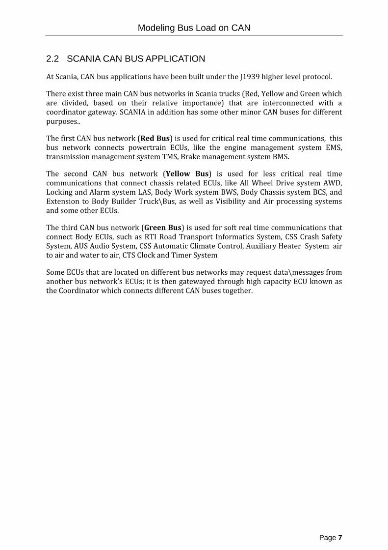
At Scania, CAN bus applications have been built under the J1939 higher level protocol.
There exist three main CAN bus networks in Scania trucks (Red, Yellow and Green which are divided, based on their relative importance) that are interconnected with a coordinator gateway. SCANIA in addition has some other minor CAN buses for different purposes..
The first CAN bus network (Red Bus) is used for critical real time communications, this bus network connects powertrain ECUs, like the engine management system EMS, transmission management system TMS, Brake management system BMS.
The second CAN bus network (Yellow Bus) is used for less critical real time communications that connect chassis related ECUs, like All Wheel Drive system AWD, Locking and Alarm system LAS, Body Work system BWS, Body Chassis system BCS, and Extension to Body Builder Truck\Bus, as well as Visibility and Air processing systems and some other ECUs.
The third CAN bus network (Green Bus) is used for soft real time communications that connect Body ECUs, such as RTI Road Transport Informatics System, CSS Crash Safety System, AUS Audio System, CSS Automatic Climate Control, Auxiliary Heater System air to air and water to air, CTS Clock and Timer System
Some ECUs that are located on different bus networks may request data\messages from another bus network’s ECUs; it is then gatewayed through high capacity ECU known as the Coordinator which connects different CAN buses together.
Modeling Bus Load on CAN
Page 8
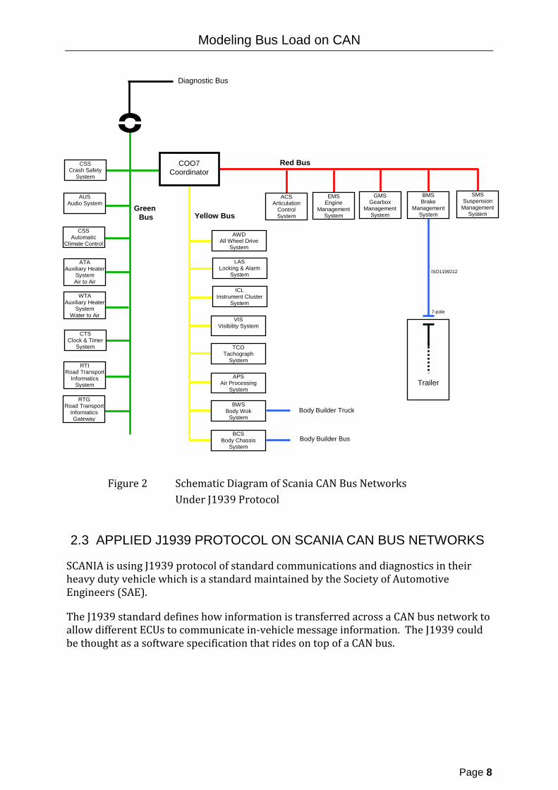
2.3 APPLIED J1939 PROTOCOL ON SCANIA CAN BUS NETWORKS
SCANIA is using J1939 protocol of standard communications and diagnostics in their heavy duty vehicle which is a standard maintained by the Society of Automotive Engineers (SAE).
The J1939 standard defines how information is transferred across a CAN bus network to allow different ECUs to communicate in-vehicle message information. The J1939 could be thought as a software specification that rides on top of a CAN bus.
Diagnostic Bus
Trailer
SMS Suspension
Management System
BMS Brake
Management System
GMS Gearbox
Management System
EMS Engine
Management System
ACS Articulation
Control System
7-pole
ISO1199212
LAS Locking & Alarm
System
ICL Instrument Cluster
System
VIS Visibility System
TCO Tachograph
System
APS Air Processing
System
BWS Body Wok
System
BCS Body Chassis
System
AWD All Wheel Drive
System
Body Builder Truck
Body Builder Bus
CSS Crash Safety
System
RTG Road Transport
Informatics Gateway
RTI Road Transport
Informatics System
CTS Clock & Timer
System
WTA Auxiliary Heater
System Water to Air
ATA Auxiliary Heater
System Air to Air
CSS Automatic
Climate Control
AUS Audio System
Red Bus
Yellow Bus Green Bus
COO7 Coordinator
Figure 2 Schematic Diagram of Scania CAN Bus Networks Under J1939 Protocol
Modeling Bus Load on CAN
Page 9
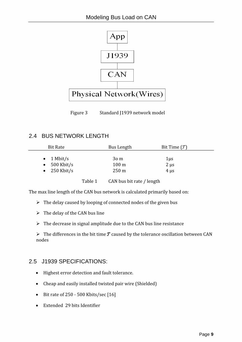
2.4 BUS NETWORK LENGTH
Bit Rate Bus Length Bit Time (𝒯)
• 1 Mbit/s 3o m 1µs • 500 Kbit/s 100 m 2 µs • 250 Kbit/s 250 m 4 µs
Table 1 CAN bus bit rate / length
The max line length of the CAN bus network is calculated primarily based on:
The delay caused by looping of connected nodes of the given bus
The delay of the CAN bus line
The decrease in signal amplitude due to the CAN bus line resistance
The differences in the bit time 𝒯 caused by the tolerance oscillation between CAN nodes
2.5 J1939 SPECIFICATIONS:
• Highest error detection and fault tolerance.
• Cheap and easily installed twisted pair wire (Shielded)
• Bit rate of 250 - 500 Kbits/sec [16]
• Extended 29 bits Identifier
Figure 3 Standard J1939 network model

Modeling Bus Load on CAN
Page 10
• Max. 30 ECUs could participate at a time in a network
• Best continuity and reliability for the above reasons
2.5.1 Message Format of J1939-21
• SOF It is a single dominant bit (start of frame, SOF) which marks the start of the frame message, and the main job for this bit is to synchronize all nodes located on the bus after idle case.
Identifier
• CAN Identifier ID The Extended CAN consists of 29 bits identifier which determines the message priority and identity.
The lower the identifier value, the higher the priority value.
• RTR It is a single remote transmission request, RTR, a dominant when another node requests information.
• DLC It is a 4 bits data length code, DLC and it contains the number of bytes of data to be transmitted.
• Data 1 Up to 64 bits of data to be transmitted.
S O F
29 Bits CAN Identifier ID
Max. 8 Bytes Data
RTR
4 Bits DLC
Contro
CRC Field 16
Bits
ACK
7 Bits EOF
Figure 4 Typical Format of J1939-21 Message
18 Bits PGN
8 Bits source address
3 Bits Priority
8 Bits PDU
Specific
8 Bits PDU
Format
1 Bit data page
1 Bit extended data page
2 Res Bits
Modeling Bus Load on CAN
Page 11
• CRC It is a 16 bits cyclic redundancy check, CRC which contains the number of transmitted bits of the data for error detection.
• ACK It is a 2 bits field, which consists of ACK slot bit and ACK delimiter
The sender of a given frame transmits both of those bits with recessive status. While the receiver, when it receives the message correctly, would send back to the sender by sending a dominant bit in the ACK Slot.
• EOF It is a 7 seven recessive bits which is known as end of frame field, EOF, and the main job is to mark the end of a frame and to disable the bit stuffing.
The 29-Bit message identifier is partitioned into three main blocks and another 4 sub blocks:
The main three blocks are:
• 3 bits Priority field which equals to 8 priority levels
• 8 bits of Source Address (source ECU)
• 18 bits of PGN, Parameter Group Number to identify the use of the PG field, which is divided into four more sub blocks:
o 1 bit extended data page.
o 1 bit for page reference, currently page1 (2 pages available)
o 8 bits of Parameter data unit Format (PF)
o 8 bits of Parameter data unit Specific (PS)
2.5.2 Translation of PF and PS contents
• When PF = 0 – 239 PDU1 refers to a destination address in PS
• When PF = 240 – 255 PDU2 refers to an extension to PDU Format PF in PS
Translation of PF and PS contentsJ1939-21 CAN Messages Arbitration

Modeling Bus Load on CAN
Page 12
2.5.3 1939-21 CAN Messages Arbitration
In the j1939 CAN bus architecture when more than one ECU starts their transmission at exactly same time after having sensing that the bus is idle, a Carrier Sense Multiple Access with Collision Avoidance CMSA/CD is applied for accessing the bus. Each message has 29 bits of ID or identifier and each ECU sends bit after bit of its identifier while monitoring the bus voltage level. As long as the transmitted bits from those ECUs are similar, nothing happens.[12]
There are two voltage levels: the first is low and called dominant and the second is high and called recessive. The dominant bits will always win the bus and at that time if the ECU which transmits the recessive bit while encountering a dominant bit in the bus, then this ECU will directly stop transmitting and wait until the bus returns to idle. Therefore at the end, only one identifier will win the arbitration and gets the bus and as a result we see that the lower the identifier, the higher the priority.
1.25
2.5
3.75
2.5 V
Volt
Time Data 1 0 1
CAN Low
CAN High
Figure 5 CAN Dominant (0) & Recessive (1) in term of Voltage

Modeling Bus Load on CAN
Page 13
2.6 STATE OF THE ART
Heavy duty vehicle manufacturers build their J1939 CAN bus networks based on common standard limitations as below:
1- Max busload utilization 80% of the CAN bus network (so that enough slack time are there for diagnostic messages, error message, overload message, etc ) [13]
2- Max. Network length of 40 meters[16]
3- Bit rate of 250 – 500 Kbits/sec[16]
4- Max. 30 ECUs could participate at a time in any given CAN bus network[16]
Manufacturers have set a standard for the setting of ‘Diagnostic Trouble Codes’, after a specific amount of time such that for wake up mode, Tdtc> Tdtc_wakeup ms while in normal running mode, Tdtc> Tdtc_normalrun if a given a message that hasn’t got into the bus network (deadlines crossed), those DTC Codes refer normally to either 1) a specific system fault or 2) simply the CAN bus has been loaded to the point that prevented a specific message from getting into the bus.
Therefore, it is recommended to examine why a given DTC Code was sat and what is the reason behind it. Searching through scientific papers did not show such a tool to
Figure 6 Typical CAN J1939 messages arbitration
Data Feild
Arbitration
29 bits identifier
CAN Bus
Message 1
Message 2
Message 3
Loss arbitration
Loss arbitration
Wins arbitration
Start of Header
Control Feild
Control Feild
Data Feild
Modeling Bus Load on CAN
Page 14
determine the breakdown utilization that helps in preventing the setting of DTC Codes (of high load reason). Instead, the case is to examine some other factors (such as priority level of a given message which sets the DTC code, or the cyclic speed of that given message) and by changing those factors, this will overcome the reason and switch off that DTC Code if the reason was a high busload which introduces latency.
2.7 CLOSELY RELATED WORK
I have referred to the following research papers which I consider the best in this field:
• Controller Area Network (CAN) Schedulability Analysis: Refuted, Revisited and Revised
Prepared by:
Robert I. Davis and Alan Burns Real-Time Systems Research Group, University of York, England
• Guaranteeing Message Latencies on Control Area Network
Prepared by:
Ken Tindell and Alan Burns, Real-Time Systems Research Group, University of York, England
• CAN Network Utilization, Busload calculations for SESAMIM – Red Bus, RESA09002 Internal Scania document
Those above papers make it possible for a researcher to get benefits from the Scheduability Analysis of CAN bus (first paper) which was developed to determine the worst case response time of any message within the CAN network and as a result it would be possible to calculate message latency (second and third papers) that are valuable in our goal towards preventing the network from falling under non schedulable network case.

Modeling Bus Load on CAN
Page 15
CHAPTER 3. LOAD ANALYSIS MODEL
To simulate and model CAN bus load, we need to show each message latency if it exists in the bus network and how much useful
free slack time is there in the network by calculating ‘alpha’ and ‘breakdown utilization’ that will be used to test a given network to determine by how much it could handle an extra load, therefore the modeling will be built up step by step.
3.1 ASSUMPTION OF MESSAGES’ ARRIVAL TIME
A worst case assumption is always the case with respect to message arrival time.
A scenario is assumed where all messages arrive at the same time, this case would introduce the longest busy period of response time for those messages.
Applying the Scheduability Analysis to calculate:
o Busy period for each message o Blocking Time for each message invocation o Waiting Time for each message invocation o Response Time for each message invocation
Calculation of messages’ latencies
Calculating the network’s breakdown parameters of ‘alpha’ & ‘breakdown utilization’
Figure 7 Flowchart of the ‘Mathematical Solution’ to model CAN bus load
END
Calculating the ‘network scheduability’
Getting Message set of a specific bus network
Calculation of ‘message transmission time’
START
Assumption of ’message arrival time’
Modeling Bus Load on CAN
Page 16
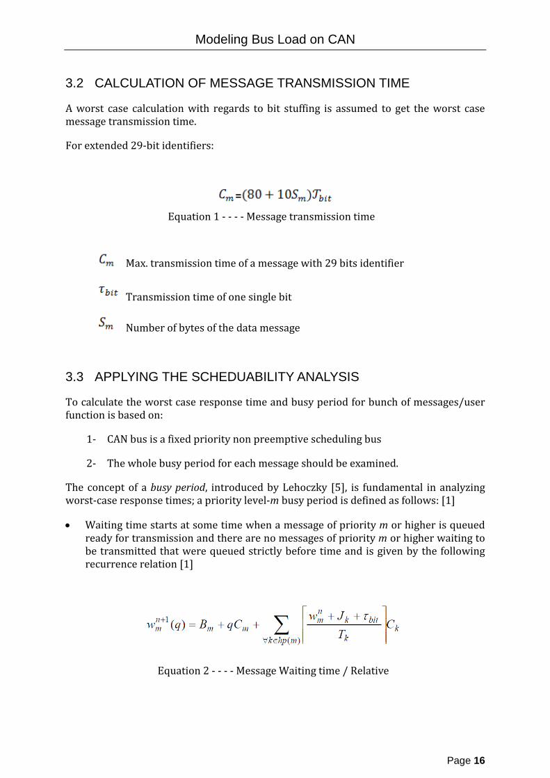
3.2 CALCULATION OF MESSAGE TRANSMISSION TIME
A worst case calculation with regards to bit stuffing is assumed to get the worst case message transmission time.
For extended 29-bit identifiers:
=
Max. transmission time of a message with 29 bits identifier
Transmission time of one single bit
Number of bytes of the data message
3.3 APPLYING THE SCHEDUABILITY ANALYSIS
To calculate the worst case response time and busy period for bunch of messages/user function is based on:
1- CAN bus is a fixed priority non preemptive scheduling bus
2- The whole busy period for each message should be examined.
The concept of a busy period, introduced by Lehoczky [5], is fundamental in analyzing worst-case response times; a priority level-m busy period is defined as follows: [1]
• Waiting time starts at some time when a message of priority m or higher is queued ready for transmission and there are no messages of priority m or higher waiting to be transmitted that were queued strictly before time and is given by the following recurrence relation [1]
Equation 1 - - - - Message transmission time
Equation 2 - - - - Message Waiting time / Relative

Modeling Bus Load on CAN
Page 17
Waiting time of the examined message m
Invocation number of the message m
Max. Blocking time of lower priority message than m
Cycle time of all higher priority messages than message m
Jitter of all higher priority messages than message m
Transmission time of all higher priority messages than message m
Transmission time of the examined message m
= Initial value
• It is a contiguous interval of time during which any message of priority lower than m (queuing time) is unable to win arbitration and to start transmission.[4]
Max. Blocking time of lower priority message than m
Transmission time of message set
• It ends at the earliest time when the bus becomes idle, ready for the next round of transmission and arbitration, yet there are no messages of priority m or higher waiting to be transmitted that were queued strictly before time . [1]
However, a higher priority message can be forced to wait for transmission when message m completes transmission and
therefore the busy period can become longer due to the fact that CAN bus does apply the Fixed priority non preemptive scheduling, therefore we have to check for multiple instances of a message m that would become ready for transmission, just before the end of the busy period is per the recursive relation below [1]:
Equation 3 - - - - Message Max. Blocking time / Relative

Modeling Bus Load on CAN
Page 18
Number of message m invocations to be examined under busy period
Busy period time of the examined message m
Jitter of examined message m
Cycle time of examined message m
• The length of the priority m message’s busy period that would be examined is given the following recurrence relation [1]
Busy period time of the examined message m
Max. Blocking time of lower priority message than m
Cycle time of all higher priority messages of m and over
Jitter of all higher priority messages of m and over
Transmission time of all higher priority messages of m and over
= Initial value
The relative response time of a priority m message for each instance is given by:
Equation 4 - - - - Number of message invoications
Equation 5 - - - - Message Busy Period

Modeling Bus Load on CAN
Page 19
Worst case response time of the examined message m
Jitter of examined message m
Waiting time of the examined message m
Transmission time of the examined message m
The worst case response time for priority m message through all invocations is given by:
Worst case response time of the examined message m
(q) Response time of the examined message m for a given invocation q
Invocation number of the message m
Number of message m invocations to be examined under busy period
3.4 CALCULATION OF LATENCY
Latency which is defined as the time remaining (which needs to be used) to finish a message execution after its deadline and
is computed for each ‘Message invocation’ during the whole of the busy period is given by:
=
Equation 6 - - - - Message Response time / Relative
Equation 7 - - - - Message worst case response time
Equation 8 - - - - Message Latency time

Modeling Bus Load on CAN
Page 20
Latency of the examined message m
Deadline time of the examined message m
Response time of the examined message m
Note: A message deadline time is assumed to be equal to cycle time of a message.
Typically, Latency for a specific message invocation is equal to the subtraction of relative deadline D for priority m message from its relative response time R.
Latency visualizing helps the User to know exactly how messages behave during the wake up mode and in the run mode which is considered one of the outcomes and goals of this thesis.
3.5 CALCULATION OF ALPHA & BREAKDOWN UTILIZATION
3.5.1 Introduction
We need to have an implementation for a performance evaluation and analysis of real-time applications based on finding breakdown utilization points. At a breakdown point the system does not fulfill the required timing constraints. This is the utilization rate where deadlines are missed for the first time. With our implementation we observe the system behind the breakdown utilization; we observe the system behavior under overload conditions.[17]
3.5.2 Definition
The value of ‘alpha’ could be defined as a relative quantity of a maximum load we could add to network until it introduces latency compared to the existed load.
3.5.3 Translation
The translation of the said definition is by having for example a network with ‘existed load= 24%’ and ‘alpha =2’ means that the breakdown point is 2x24% = 48%
a value of alpha close to but greater than 1 indicates that although the system is schedulable, there is little room for increasing the load. The 0 value for alpha for the bus speed indicates that no value for breakdown utilization can be found (a non schedulable system) [2]
‘alpha’ is an indication factor of how much useful free slack time there is in the network which an extra load could benefit from until network introduces latency, it is a maximum value such that when the message periods are divided by alpha the system remains schedulable (i.e. all latency requirements are met). [5]

Modeling Bus Load on CAN
Page 21
3.5.4 Possibilities
alpha=0 A non schedulable system, no value for breakdown utilization can be found
alpha=1 A schedulable system and there is no useful room for increasing the load.
alpha>1 The system is schedulable, and there is a useful room for increasing the load based on the how much alpha is greater than 1. (The greater the ‘alpha’, the greater the useful free slack time in the network, the greater the load we could add)
3.5.5 Modeling
We start a new simulation by running the scheduability analysis and checking the scheduability of a network after another, If the system is schedulable (the normal case), then we start by dividing each message cycle in a given bus network with step counter called Beta (started with 1 and increased with a counter ‘resolution’ of 0.1) then we run the mathematical scheduability analysis and check results, if the latency requirements still met, continue by increasing the step counter and running the mathematical scheduability analysis and check results until the latency introduced in the bus.
The value of that step counter at this point is our targeted ‘alpha’ of that bus and the bus utilization at this point is the ‘Breakdown Utilization’ of that bus.
if the given network is not schedulable (the non-normal case), then its associated ‘alpha’ is equal to zero (a non schedulable system).
Breakdown utilization is the bus breakdown point, which happens when the bus starts to introduce latencies, and computed by the percentage of max
3.6 FURTHER BUSLOAD
throughput (achieved using alpha point) over the bus bit rate.
Normally, modeling of the CAN busload will not take into account the diagnostic messages load on the bus. Most of those messages are only allowed when the vehicle is in ‘’still’’ mode. For KWP and UDS diagnostic messages, we locate the server cycle to each diagnostic message (sporadic message), however it is difficult to calculate their exact load because it depend on how many servers do we intend to initiate and how many commands will we activate at a time, but in reality there are a minimum of two servers initiated at a time which are sending multi packet messages with transport protocol and
The error messages load on the bus would be neglected in calculation, error messages are initiated when one node in the bus discovers an error in the incoming message, because of bit error rate BER in CAN bus is equal to 3*10-11 , which could be approximated to zero [13].
therefore their load could be. 2tp * 20 fr/s * 155 bit/fr * 4µs/bit = 0.0248 = 2.48% extra load (in still mode). [8]
Messages with a sporadic nature, such as request messages (which are not allowed at all in the Scania red bus) would be also neglected in the busload calculations, due to the fact that their load is approximated to zero [9]

Modeling Bus Load on CAN
Page 22
CHAPTER 4. FLOWCHART OF TOOL FUNCTIONS
<1
No Schedule could be determined Code stop test & simulation Equations and formulas are only applicable to a bus network of Load Utilization <1
>1 Run the Simulation for the desired Period (total)
Test messages of the given bus Using (The Mathematical Scheduability Analysis) to determine for each message:
Busy period BP Total message invocations to test based on BP Blocking Time B for each message invocation Waiting Time W for each message invocation Latency for each message invocation Response Time R for each message invocation Worst case response time
Pushbutton/Function 3 BreakDown Parameters is to produce an xls file
with a name ‘Breakdown’ which contains a
breakdown analysis of all buses under test, ,
including:.
Figure 8 Flowchart of CAN Tool code to model bus load on CAN
Pushbutton/Function 1 Plotting To plot out on bmp files series of bus models, each one belong to a different bus network In each plot, the following parameters are plotted including: response time for each message invocation
in the busy period latency for each message invocation in the
busy period cycle time, for each message invocation in
the busy period deadline time, for each message invocation
in the busy period
Getting buses into test and simulation in successive
bases (J)
Pushbutton/Function 2 Response Time Analysis
To produce a xls file called ‘ResponseTime’ which contains tables of Response Time Analysis of the messages of all networks under test., including: Latency for each message invocation Response Time R for each message invocation Worst case response time Busy period long Total message invocations to test based on BP Bus Load Utilization
Pushbutton Selector
By selecting ‘Stop’ Simulation mode at the beginning, the User will be able to interrupt the simulation, while the Tool would be in WAIT mode, then the User will get all TTR reports printed in excel, so he can add, remove or modify any message attribute he may want and then resume simulation and modeling by changing Simulation Mode to ‘Resume’.
Initiate a Graphical User Interface (GUI) named CAN_TOOL.exe It allows the user to easily interact with the MODELING TOOL and to enter the desired input parameters, log files and databases. Also, User to enter the details of the messages that will be added, removed or modified to check the network behavior after test simulation, It has the following Pushbutton functions:
1- RUN (The Main Function) 2- Response Time Analysis 3- Break Down Parameters 4- Plotting
Push the main pushbutton (RUN) It would get the interface input parameters and then run CAN_App Accessing of Scania CAN database
and defining all busses & messages parameters incl. name, type, priority, timing parameters,.. etc by calling function mydatabase that access different Scania CAN databases (tool accept more database inputs )
Defining of the time resolution of the test simulation (resolution) & the total simulation time (total)
Code Admission Control Check utilization of
the given bus

Modeling Bus Load on CAN
Page 23
CHAPTER 5. GRAPHICAL USER INTERFACE GUI
I chose to use a Graphical User Interface as a human-CAN_Tool interface (i.e., a way for humans to interact with computers) that uses windows, icons and menus and which can be manipulated by a mouse. [15]
5.1 THE TOOL’S INPUT
The Interface is stimulated with 28 inputs which varies from bit rate to message parameter to file names, including three panels for adding, removing or modifying a specific message or bench of messages.
The input consists of:
1- Data Log File is a log file that resulted from testing with CANalyzer that contains all possible CAN message logs in the network during the period of test and it should be in xlsx file format.
Very small Input Sample of data logs
Time 0.000000
Bus 1
Message ID CF00400x
0.000272 1 8FE6E0Bx 0.000284 3 CFE5A27x 0.000274 1 CFE6CEEx 0.000282 2 CFF8100x 0.004805 1 18FE592Fx 0.000484 1 18E520C8x 0.000352 3 18FEC4C8x 0.000364 1 18FEC6C8x 0.000906 2 CF00203x 0.000286 1 C040B03x 0.001720 2 CFFA700x 0.000758 1 CFF8027x 0.000280 1 C040B11x 0.000276 1 18F0090Bx 0.006184 3 CF00203x 0.000282 1 18FFA103x 0.002102 2 CFE6CEEx 0.000282 3 CF00400x 0.000272 3 8FE6E0Bx 0.000270 1 CFF9111x 0.000286 2 18E4A827x 0.000290 3 18FECA00x
2- Diagnostic Log File is a log file that resulted from testing with CANalyzer while initiating of all possible diagnostic functions, it should be in xlsx file format.
3- Network Database file is a database file that contains all possible CAN messages along with its name, attribute, ID, source node, arbitration field and message type and transmitter ECU, this file is come in xls format.

Modeling Bus Load on CAN
Page 24
4- The simulation mode allows User to interrupt the simulation, while the Tool will be on wait
5- Network Baud rate is a Popupmenus to select a baud rate of a specific network.
, then User will get all TTR reports printed in excel on newly created folder, so he can add, remove or modify any message attribute he may want and then resumes simulation and modeling by changing Simulation Mode to ‘Resume Mode’ in the main tool’s dashboard.
5.2 THE TOOL’S OUTPUT
Refer to figure 9 of the CAN TOOL Interface, there are seven pushbuttons
The first (Main) pushbutton (RUN) to run the modeling and mathematical solution
in the Interface:
The second pushbutton (Plotting) is to plot out the models for each bus on bmp files
The third pushbutton (Breakdown Parameters) is to produce an xls file with a name ‘Breakdown.xls’ which contains a breakdown analysis of all tested buses.
The forth pushbutton (Response Time Analysis) is to produce an xls file called ‘ResponseTime.xls’ which contains tables of Response Time Analysis of all message of each of the targeted bus networks.
The fifth pushbutton (Help & Support), clicking on this pushbutton will show a list of topics to get help on each one by selecting with mouse.
The sixth pushbutton (Delete O/P) is to delete the produced excel TTR xls files & Breakdown/response time analysis txt files.
The seventh pushbutton (Contact), clicking on this pushbutton will show contact details of the producer.

Modeling Bus Load on CAN
Page 25
SCANLA (The developed CAN busload modeling tool) is running from executable
application and could be installed on different computers direct from one single .exe
application file.
It is able to map different CAN bus log files that resulted of testing with CANalyzer, such
that the tool is digging deep into those log files and searches all possible data inside
them to locate and analyze all messages, even if those log files contained hundreds of
thousands of messages logs
Also it is able to access Scania CAN database and define all busses & messages
parameters including name, type, priority, timing parameters, Etc.
SCANLA (
The developed CAN busload modeling tool) is running from executable application and could be installed on different computers direct from one single .exe application file.
It is able to map different CAN bus log files that resulted of testing with CANalyzer, such that the tool is digging deep into those log files and searches all possible data inside them to locate and analyze all messages, even if those log files contained hundreds of thousands of messages logs
Also it is able to access Scania CAN database and define all busses & messages parameters including name, type, priority, timing parameters, Etc.
Figure 9 Snapshot of the Produced Human –CAN_TOOL Interface using of GUI Simulation Mode
Tool’s Pushbuttons Tool Name and Version Main Input Edit Fields
Networks’ Baud Rates Popupmenus

Modeling Bus Load on CAN
Page 26
Figure 10 Sample of the red bus traffic report. (Produced by the tool)
Figure 10 is built by analyzing data log file and mapped to CAN red database file and contains message name, message ID, source node, relative priority, cycle time and message type. Note that these reports could be modified by the user to build a simulation that matches his own desire.
Figure 11 Sample of the red bus response time analysis (Produced by the tool)

Modeling Bus Load on CAN
Page 27
Figure 11 is built by applying our mathematical solution to the data set of figure 10 in order to calculate response time analysis of those data set including busy period length, waiting time, blocking time response time and latency
Figure 12 Sample of the different networks’ breakdown point (Produced by the tool)
Figure 12 is a showing the bus utilization of those networks tested in figure 10 and 11 and their respective breakdown utilization points.
Figure 13 Sample of a green bus latency/response time plot (Produced by the tool)
Figure 13 shows plot of message response time and message latency in logarithmic scale of millimeters of each message invocations during busy period of those messages tested in figures 10, 11 and 12

Modeling Bus Load on CAN
Page 28
CHAPTER 6. TEST RESULTS & ANALYSIS
The TTR BENCHMARK, (based on Scania T vehicle LOG FILES done by CANalyzer test on March 22, 2012) is a report describing a set of more than 200 messages of a specific Scania vehicle (Scania T vehicle) hardware configuration sent between multiple subsystems in three CAN bus networks (Red, Yellow and Green Scania CAN Buses) gatewayed with a powerful ECU known as the coordinator. Note that Scania deals with different combinations of those subsystems and associated messages.
There exist 19 subsystems equipped in the Scania T Vehicle as per the following:
Suspension Management System SMS, Brake Management System BMS, Gearbox Management System GMS, Engine Management System EMS, Articulation Control System ACS, All Wheel Drive System AWD, Locking and Alarm System LAS, Instrument Cluster System ICS, Visibility System VIS, Tachograph System TCS, Air Processing System APS, Body Wok System BWS, Body Chassis System BCS, Coordinator COO7, Crash Safety System CSS, Audio System AUS, Automatic Climate Control ACC, Air to Air Auxiliary Heater System ATA, Water to Air Auxiliary Heater System WTA, Clock and Timer System CTS, Road Transport Informatics System RTS, Road Transport Informatics Gateway RTG
The CAN networks connecting those ECU subsystems are required to handle more than 200 messages, some of them come with sporadic nature, while most are considered control data with fixed periodic nature and absolutely, the latency should be kept less than an associated period. While the sporadic messages do have an offline latency requirement that has been fixed prior to network setup, for instance all messages that are sent due to the driver interaction to get a latency requirement of 25ms[2], that would imply the response should show up to the driver immediately. Any given sporadic message should be given a period that represents a maximum inter arrival rate at the rate they may occur). [3]
Appendix 1 shows the TTR Benchmark tables of Scania T vehicle Red, Yellow and Green bus network (messages’ requirements in order to get scheduled), those messages, some of them do have fixed periodic, but some do come sporadically in response to an external or internal event).

Modeling Bus Load on CAN
Page 29
6.1 TEST 1, A REALISTIC TEST BASED ON CAN LOG FILE FROM T VEHICLE
The following TEST details the results of running our CAN TOOL resulting from analyzing data from the log file of SCANIA T Vehicle
Figure 15 Response Time (Test1) of Red Bus Messages Invocation 1
(BP ends at 1st invocation)
Figure 14 Response Time (Test1) of Green Bus Messages Invocation 1
(BP ends at 1st invocation)

Modeling Bus Load on CAN
Page 30
Figure 16 Response Time (Test1) of Yellow Bus Messages Invocation 1 (BP ends at 2nd invocation)
Figure 17 Response Time (Test1) of Yellow Bus Messages Invocation 2 (BP ends at 2nd invocation)
Message X46 introduces Latency, Deadline is not met

Modeling Bus Load on CAN
Page 31
6.1.1 Resulted Breakdown Utilization & alpha
Bus Bus Utilization alpha Breakdown Utilization
Red 34.29 1.50 51.4383 Yellow 46.62 0.00 00.0000 Green 20.71 2.20 45.5576
Table 2 Test1 Resulted Breakdown Utilization & alpha
Alpha does detail the breakdown utilization of the system for the given bus speed. While the breakdown utilization is the largest value of alpha such that when all the message periods are divided by alpha the system remains schedulable (i.e. all latency requirements are met).
It is an indication of how much slack there is in the system: a value of alpha close to but greater than 1 indicates that although the system is schedulable, there is little room for increasing the load. The 0 value for alpha for the bus speed indicates that no value for breakdown utilization can be found (an unschedulable system)
6.1.2 Encountered Latencies
In figure 12 of the Yellow bus response time plot, we have notice that the following message (refer to Appendix 1)
Message Name X46
Message ID 0x18FFXXXX
This Message does not meet deadline requirements and is not able to seize the bus in the desired cycle time, and it introduced latency.
Note: Message to control/send information to any type of GMS (AWD included)
6.1.3 Suggested Solution
Repairing the said network breakdown could be done by modifying either the cycle time (not preferred due to strict timing behavior of its signals) or modifying the message priority level (relatively preferred).
Message Name ‘X46’
Message ID 0x18FFXXXX
Raising the Priority of Message ‘X46’ 0x0CFFXXXX

Modeling Bus Load on CAN
Page 32
6.2 RUNNING TEST 2 ON THE REPAIRED YELLOW BUS
The following tables and charts resulted from rerunning the CAN TOOL with the new modified message X46 priority level in the yellow bus network
6.2.1 Resulted Breakdown Utilization & alpha
Bus Bus Utilization alpha Breakdown Utilization
Yellow 46.62 1.50 69.9360
Table 3 Test2 Resulted Breakdown Utilization & alpha
6.2.2 Discussion
We have seen in test 1 that although yellow bus utilization is relatively low, look at table 2 (about 46%), the breakdown utilization is reached and bus network starts to introduce latency, using the tool enabled us to visualize and locate the reason behind that breakdown, it is a critical real time message called X46 which has a fast cycle and a relative low priority.
The tool was helpful in repairing the said network breakdown, by modifying either the cycle time (not preferred due to strict timing behavior of its signals) or modifying the message priority level (relatively preferred).
Figure 18 Response Time (Test2) of Yellow Bus Messages Invocation 1
(BP ends at 1st invocation)

Modeling Bus Load on CAN
Page 33
6.3 REFERENCE TEST
The following Test details the results of running the CAN TOOL by stimulating with all possible messages of SCANIA T Vehicle into RED BUS with a lower to half bus bit rate.
Note: The purpose of this test is to visualize the response time of red bus messages when the bit rate decreased to the half of its value, the response time in this case would be one more piece of evidence of how far the network is from the breakdown point.
Figure 19 Response Time (Ref. Test) of Red Bus Messages Invocation 1 (BP ends at 2nd invocation)
Figure 20 Response Time (Ref. Test) of Red Bus Messages Invocation 2 (BP ends at 2nd invocation)
Message X120, X105, &X46 introduce Latencies Deadlines are not met
Modeling Bus Load on CAN
Page 34
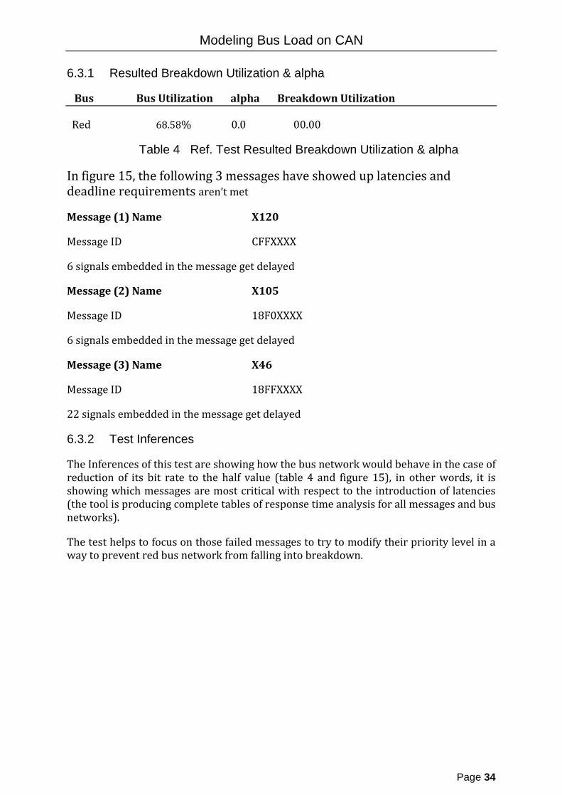
6.3.1 Resulted Breakdown Utilization & alpha
Bus Bus Utilization alpha Breakdown Utilization
Red 68.58% 0.0 00.00
Table 4 Ref. Test Resulted Breakdown Utilization & alpha
In figure 15, the following 3 messages have showed up latencies and deadline requirements aren’t met
Message (1) Name X120
Message ID CFFXXXX
6 signals embedded in the message get delayed
Message (2) Name X105
Message ID 18F0XXXX
6 signals embedded in the message get delayed
Message (3) Name X46
Message ID 18FFXXXX
22 signals embedded in the message get delayed
6.3.2 Test Inferences
The Inferences of this test are showing how the bus network would behave in the case of reduction of its bit rate to the half value (table 4 and figure 15), in other words, it is showing which messages are most critical with respect to the introduction of latencies (the tool is producing complete tables of response time analysis for all messages and bus networks).
The test helps to focus on those failed messages to try to modify their priority level in a way to prevent red bus network from falling into breakdown.
Modeling Bus Load on CAN
Page 35
CHAPTER 7. MODELING OF DIAGNOSTIC LOAD
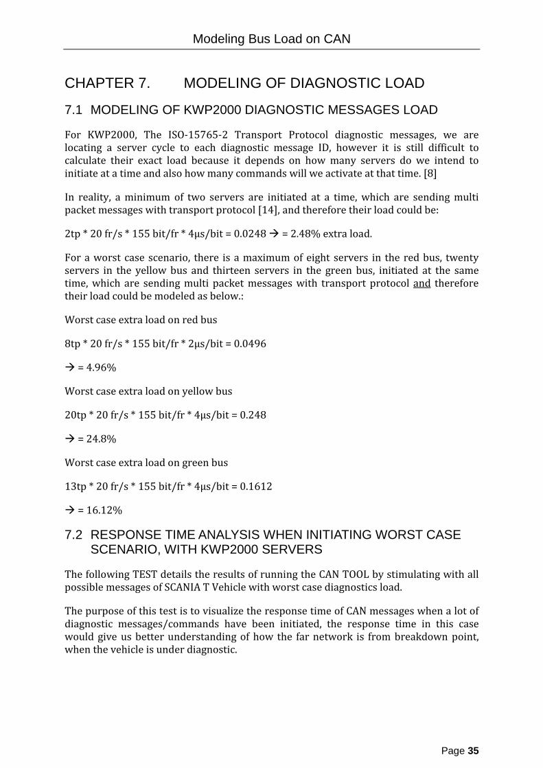
7.1 MODELING OF KWP2000 DIAGNOSTIC MESSAGES LOAD
For KWP2000, The ISO-15765-2 Transport Protocol diagnostic messages, we are locating a server cycle to each diagnostic message ID, however it is still difficult to calculate their exact load because it depends on how many servers do we intend to initiate at a time and also how many commands will we activate at that time. [8]
In reality, a minimum of two servers are initiated at a time, which are sending multi packet messages with transport protocol [14], and therefore their load could be:
2tp * 20 fr/s * 155 bit/fr * 4µs/bit = 0.0248 = 2.48% extra load.
For a worst case scenario, there is a maximum of eight servers in the red bus, twenty servers in the yellow bus and thirteen servers in the green bus, initiated at the same time, which are sending multi packet messages with transport protocol and
Worst case extra load on red bus
therefore their load could be modeled as below.:
8tp * 20 fr/s * 155 bit/fr * 2µs/bit = 0.0496
= 4.96%
Worst case extra load on yellow bus
20tp * 20 fr/s * 155 bit/fr * 4µs/bit = 0.248
= 24.8%
Worst case extra load on green bus
13tp * 20 fr/s * 155 bit/fr * 4µs/bit = 0.1612
= 16.12%
7.2 RESPONSE TIME ANALYSIS WHEN INITIATING WORST CASE SCENARIO, WITH KWP2000 SERVERS
The following TEST details the results of running the CAN TOOL by stimulating with all possible messages of SCANIA T Vehicle with worst case diagnostics load.
The purpose of this test is to visualize the response time of CAN messages when a lot of diagnostic messages/commands have been initiated, the response time in this case would give us better understanding of how the far network is from breakdown point, when the vehicle is under diagnostic.

Modeling Bus Load on CAN
Page 36
Critical Messages X120, X105, &X46 are on the edge of introducing Latencies A small extra load would push them to introduce latencies
Critical Message KWP2000Phys_L8 (Diagnostic Message)
is on the edge of introducing Latency A small extra load would push it to introduce latency
Figure 21 Response Time (Diagnostic Test) of Red Bus Messages Invocation 1 (BP ends at 1st invocation)
Figure 22 Response Time (Diagnostic Test) of Green Bus Messages Invocation 1 (BP ends at 1st invocation)
Modeling Bus Load on CAN
Page 37
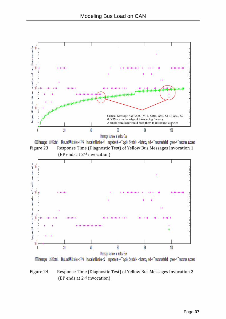
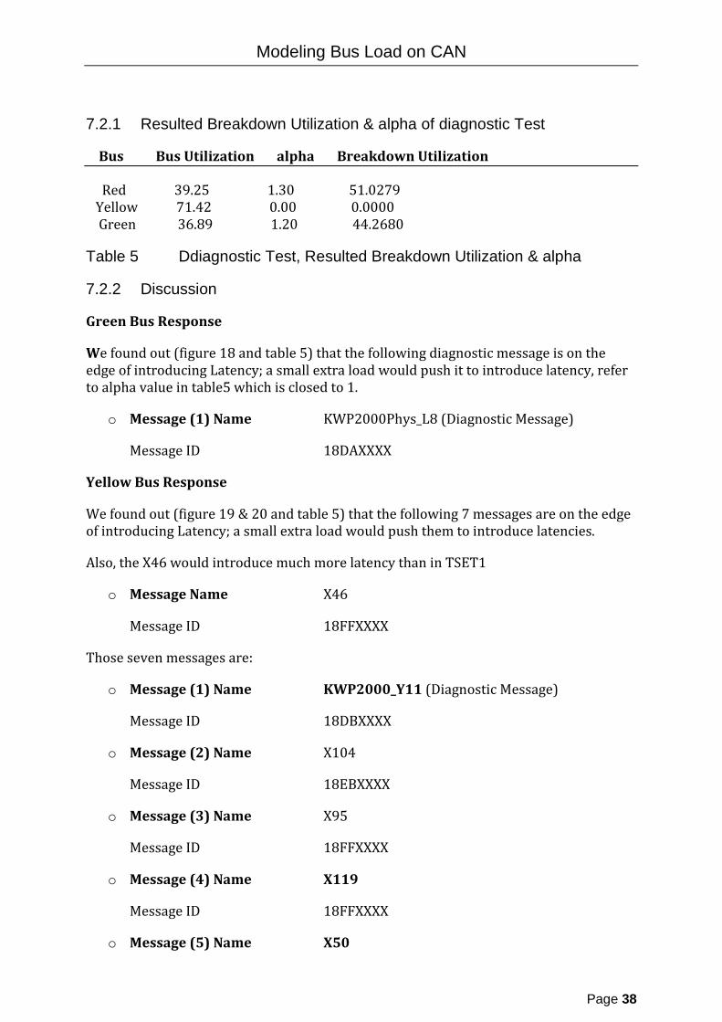
Critical Message KWP2000_Y11, X104, X95, X119, X50, X2 & X55 are on the edge of introducing Latency A small extra load would push them to introduce latencies
Figure 23 Response Time (Diagnostic Test) of Yellow Bus Messages Invocation 1 (BP ends at 2nd invocation)
Figure 24 Response Time (Diagnostic Test) of Yellow Bus Messages Invocation 2 (BP ends at 2nd invocation)
Modeling Bus Load on CAN
Page 38
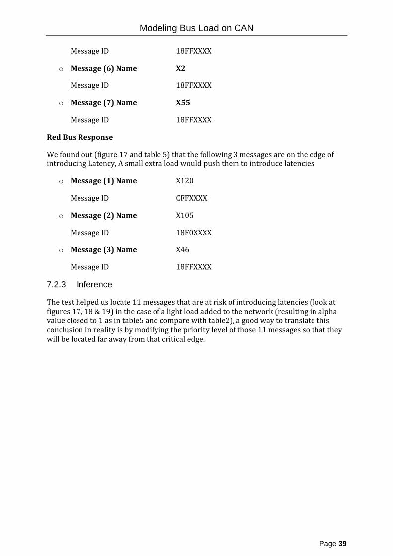
7.2.1 Resulted Breakdown Utilization & alpha of diagnostic Test
Bus Bus Utilization alpha Breakdown Utilization
Red 39.25 1.30 51.0279 Yellow 71.42 0.00 0.0000 Green 36.89 1.20 44.2680
Table 5 Ddiagnostic Test, Resulted Breakdown Utilization & alpha
7.2.2 Discussion
Green Bus Response
We found out (figure 18 and table 5) that the following diagnostic message is on the edge of introducing Latency; a small extra load would push it to introduce latency, refer to alpha value in table5 which is closed to 1.
o Message (1) Name KWP2000Phys_L8 (Diagnostic Message)
Message ID 18DAXXXX
Yellow Bus Response
We found out (figure 19 & 20 and table 5) that the following 7 messages are on the edge of introducing Latency; a small extra load would push them to introduce latencies.
Also, the X46 would introduce much more latency than in TSET1
o Message Name X46
Message ID 18FFXXXX
Those seven messages are:
o Message (1) Name KWP2000_Y11 (Diagnostic Message)
Message ID 18DBXXXX
o Message (2) Name X104
Message ID 18EBXXXX
o Message (3) Name X95
Message ID 18FFXXXX
o Message (4) Name X119
Message ID 18FFXXXX
o Message (5) Name X50
Modeling Bus Load on CAN
Page 39
Message ID 18FFXXXX
o Message (6) Name X2
Message ID 18FFXXXX
o Message (7) Name X55
Message ID 18FFXXXX
Red Bus Response
We found out (figure 17 and table 5) that the following 3 messages are on the edge of introducing Latency, A small extra load would push them to introduce latencies
o Message (1) Name X120
Message ID CFFXXXX
o Message (2) Name X105
Message ID 18F0XXXX
o Message (3) Name X46
Message ID 18FFXXXX
7.2.3 Inference
The test helped us locate 11 messages that are at risk of introducing latencies (look at figures 17, 18 & 19) in the case of a light load added to the network (resulting in alpha value closed to 1 as in table5 and compare with table2), a good way to translate this conclusion in reality is by modifying the priority level of those 11 messages so that they will be located far away from that critical edge.

Modeling Bus Load on CAN
Page 40
CHAPTER 8. CONCLUSIONS
The CAN Tool developed in this thesis which run as an executable application and based on MATLAB programming environment proved its ability to model busload for all possible Scania bus networks, ECU and messages combinations (by showing identical
The Tool achieved modeling and visualizing messages latencies for each message invocation during the whole of a busy period.
results with another results measured by SCANIA Test Department).
The Tool is able to determine and predict based on mathematical calculation, breakdown points for any given CAN bus network along with some other breakdown parameters, actually the tool can run a simulation for a huge number of messages and for multiple buses on a parallel basis.
The CAN tool is able to access Scania CAN databases to define the whole buses and messages attributes and parameters, and avoiding stimulating them manually in order to keep the whole thing running automatically.
The CAN Tool is built with Graphical User Interface as a human-computer interface. A major advantage of GUIs is that it makes computer operation more intuitive.
The CAN Tool is able to map different CAN bus log files a result of testing with CANalyzer, such that the tool is digging deep into those log files and searches all possible data inside them to locate and analyze all messages with their actual response time and IDs, even if those log files contained hundreds of thousands of messages logs, such as the one we used in Test1.
8.1 SUGGESTIONS TO FUTURE WORK
I consider the tool resulting from this thesis as a preliminary modeling towards future development of another tool to model multiple in-vehicle serial bus communication networks into one single simulator to monitor how each single traffic behaves in different combinations of vehicles, communication modes and traffic design parameters.

Modeling Bus Load on CAN
Page 41
REFERENCES [1] Controller Area Network (CAN) Schedulability Analysis: Refuted, Revisited and Revised, Robert I. Davis and Alan Burns Real-Time Systems Research Group, University of York, England
[2] GUARANTEEING MESSAGE LATENCIES ON CONTROL AREA NETWORK, Ken Tindell & Alan Burns, Real-Time Systems Research Group, University of York, UK
[3] Kopetz, H., “A Solution to an Automotive Control System Benchmark”,Technische Universität Wien, research report 4/1994 (April 1994)
[4] M.G. Harbour, M.H. Klein, J.P. Lehoczky. “Fixed priority scheduling of periodic tasks with varying execution priority” In 18 Proceedings 12th IEEE Real-Time Systems Symposium, pp. 116-128, IEEE Computer Society Press, December 1991
[5] J. Lehoczky. “Fixed priority scheduling of periodic task sets with arbitrary deadlines”. In Proceedings 11th IEEE Real-Time Systems Symposium, pp. 201–209, IEEE Computer Society Press, December 1990.
[6] MathWork usage, http://www.mathworks.se/products/matlab/
[7] Modeling and Simulation of Systems Using MATLAB and Simulink, By: Devendra K. Chaturvedi
[8] CAN Network Utilization, Busload calculations for SESAMIM – Red Bus, RESA09002 Internal Scania doc.
[9] Data communication requirements & control units by Magnus Gustavsson, TB4262, Internal Scania doc.
[10]Technical Product Data, BY Jonny Johansson, nr 1443613, Internal Scania document.
[11] CAN (Controller Area Network) Bus Communication System Based on Matlab/Simulink, Author: Fang Li , Issue Date : 12-14 Oct. 2008,
[12] Evaluation and Comparison of the Real-Time Performance, of CAN A.Albert, Gerth
[13] Vehicle data acquisition using CAN, By Henning Olsson, 8801 East Hampden Avenue Suite 210, Denver, Colorado, 80231 USA
[14] Keyword Protocol 2000 KWP2000, SSF 14230, Implementation Standard Road Vehicles - Diagnostic Systems, Author: L. Magnusson Mecel AB
[15] The Linux Information Project, GUI Definition, http://www.linfo.org.
[16] SAE J1939/11 Physical Layer
[17] Application Oriented Performance Evaluation of Real-Time Systems Based on Modern Microprocessor Architectures, Frank Golatowski, University of Rostock, Department of Electrical Engineering, Institute of Applied Microelectronics and Computer Science
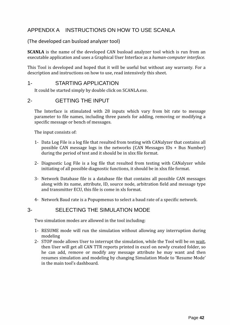
Page 42
APPENDIX A INSTRUCTIONS ON HOW TO USE SCANLA (The developed can busload analyzer tool)
SCANLA is the name of the developed CAN busload analyzer tool which is run from an executable application and uses a Graphical User Interface as a human-computer interface.
This Tool is developed and hoped that it will be useful but without any warranty. For a description and instructions on how to use, read intensively this sheet.
1- STARTING APPLICATION It could be started simply by double click on SCANLA.exe.
2- GETTING THE INPUT
The Interface is stimulated with 28 inputs which vary from bit rate to message parameter to file names, including three panels for adding, removing or modifying a specific message or bench of messages.
The input consists of:
1- Data Log File is a log file that resulted from testing with CANalyzer that contains all possible CAN message logs in the networks (CAN Messages IDs + Bus Number) during the period of test and it should be in xlsx file format.
2- Diagnostic Log File is a log file that resulted from testing with CANalyzer while initiating of all possible diagnostic functions, it should be in xlsx file format.
3- Network Database file is a database file that contains all possible CAN messages along with its name, attribute, ID, source node, arbitration field and message type and transmitter ECU, this file is come in xls format.
4- Network Baud rate is a Popupmenus to select a baud rate of a specific network.
3- SELECTING THE SIMULATION MODE
Two simulation modes are allowed in the tool including:
1- RESUME mode will run the simulation without allowing any interruption during modeling
2- STOP mode allows User to interrupt the simulation, while the Tool will be on wait
, then User will get all CAN TTR reports printed in excel on newly created folder, so he can add, remove or modify any message attribute he may want and then resumes simulation and modeling by changing Simulation Mode to ‘Resume Mode’ in the main tool’s dashboard.

Page 43
4- RUNNING THE ANALYSIS TOOL
This could be done easily by clicking on the ‘RUN’ pushbutton and only after finishing with steps 1 and 2.
Snapshot of SCANLA The developed CAN busload analyzer
Functionality Pushbuttons Tool’s Name
& Version
Networks’ Baud Rates
Main Input Edit Fields
Simulation Mode
Tool’s Help & Support

Page 44
5- PRODUCING THE OUTPUT
Refer to tool’s Interface figure; there are seven pushbuttons
The first and main pushbutton (RUN) is to run the modeling and mathematical solution as the first stage of in our tool (second, third and fourth pushbuttons are only allowed after finishing with RUN).
in the Interface:
The second pushbutton (Plotting) is to plot out models for each bus on bmp files
The third pushbutton (Breakdown Parameters) is to produce an xls file with a name ‘Breakdown.xls’ which contains a breakdown analysis of all tested buses.
The forth pushbutton (Response Time Analysis) is to produce an xls file called ‘ResponseTime.xls’ which contains tables of Response Time Analysis of all message of each of the targeted bus networks.
The fifth pushbutton (Help & Support), clicking on this pushbutton will show a list of topics to get help on each one by selecting with mouse.
The sixth pushbutton (Delete O/P) is to delete the produced excel TTR xls files, Breakdown txt file, response time analysis txt file and the plot bmp files.
The seventh pushbutton (Contact), clicking on this pushbutton will show contact details of the producers.
Note that for each simulation run, an automatic simulation unique number and date are stamped for archiving purpose.
SCANLA is the name of the developed CAN busload analyzer tool in this thesis which is running as an executable application and uses a Graphical User Interface as a human-computer interface.
Please let the producers of the mentioned tool know of any improvements, changes or modifications that might be made. <[email protected]>

Page 45
APPENDIX B SCANIA T, CAN TRAFFIC TTR REPORTS

Page 46
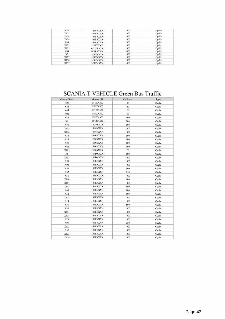
Page 47

Page 48
APPENDIX C SCANIA T, CAN RESSPONSE TIME ANALYSIS

Page 49

Page 50