University of Kentucky University of Kentucky

UKnowledge UKnowledge

University of Kentucky Master's Theses Graduate School

2005

MODELING AND TESTING ULTRA-LIGHTWEIGHT THERMOFORM-MODELING AND TESTING ULTRA-LIGHTWEIGHT THERMOFORM-

STIFFENED PANELS STIFFENED PANELS

Prathik Navalpakkam University of Kentucky, prathik@engr.uky.edu

Right click to open a feedback form in a new tab to let us know how this document benefits you. Right click to open a feedback form in a new tab to let us know how this document benefits you.

Recommended Citation Recommended Citation Navalpakkam, Prathik, "MODELING AND TESTING ULTRA-LIGHTWEIGHT THERMOFORM-STIFFENED PANELS" (2005). University of Kentucky Master's Theses. 350. https://uknowledge.uky.edu/gradschool_theses/350

This Thesis is brought to you for free and open access by the Graduate School at UKnowledge. It has been accepted for inclusion in University of Kentucky Master's Theses by an authorized administrator of UKnowledge. For more information, please contact UKnowledge@lsv.uky.edu.

ABSTRACT OF THESIS

MODELING AND TESTING ULTRA-LIGHTWEIGHT

THERMOFORM-STIFFENED PANELS

Ultra-lightweight thermoformed stiffened structures are emerging as a viable option for spacecraft applications due to their advantage over inflatable structures. Although pressurization may be used for deployment, constant pressure is not required to maintain stiffness. However, thermoformed stiffening features are often locally nonlinear in their behavior under loading. This thesis has three aspects: 1) to understand stiffness properties of a thermoformed stiffened ultra-lightweight panel, 2) to develop finite element models using a phased-verification approach and 3) to verify panel response to dynamic loading. This thesis demonstrates that conventional static and dynamic testing principles can be applied to test ultra-lightweight thermoformed stiffened structures. Another contribution of this thesis is by evaluating the stiffness properties of different stiffener configurations. Finally, the procedure used in this thesis could be adapted in the study of similar ultra-lightweight thermoformed stiffened spacecraft structures. KEYWORDS: Thermoformed stiffened panels, conical stiffener units, modal testing

Prathik Navalpakkam November 2005

MODELING AND TESTING ULTRA-LIGHTWEIGHT

THERMOFORM-STIFFENED PANELS

By

Prathik Navalpakkam

Director of Graduate Studies

Director of Thesis

Date

RULES FOR THE USE OF THESES

Unpublished theses submitted for the Master’s degree and deposited in the University of Kentucky Library are as a rule open for inspection, but are to be used only with due regards of the rights of the authors. Bibliographical references may be noted, but with quotations or summaries of parts may be published only with the permission of the author, and with the usual scholarly acknowledgements. Extensive copying or publication of the thesis in whole or in part also requires the consent of the Dean of the Graduate School of the University of Kentucky.

THESIS

Prathik Navalpakkam

The Graduate School

University of Kentucky

2005

MASTER’S THESIS RELEASE

I authorize the University of Kentucky Libraries to reproduce this thesis in whole or in part

for purposes of research

Signed: _______________

Date: _______________

MODELING AND TESTING ULTRA-LIGHTWEIGHT THERMOFORM-

STIFFENED PANELS

THESIS

A thesis submitted in partial fulfillment of the requirements for the

degree of Master of Science in Mechanical Engineering at the

University of Kentucky

By

Prathik Navalpakkam

Director: Dr. Suzanne W. Smith, Professor of Mechanical Engineering

Lexington, KY

2005

ACKNOWLEDGEMENTS

This thesis would not have been completed without the support and

encouragement of Dr. Suzanne Weaver Smith, my Thesis Chair and Academic Advisor. I

would like to thank her with utmost sincerity and will remain obliged to her for her

motivation and guidance.

I would like to thank Dr. Keith Rouch for being a member of my graduate

committee and providing guidance in finite element analysis. I would like to thank Dr.

John Baker for his time and for being a member of my committee.

I am greatly indebted to United Applied Technologies for providing panel test

samples used for this work. I owe special gratitude to Mr. Larry Bradford, President,

United Applied Technologies for the same.

I would like to convey my thanks to all the members of Dynamic Structures and

Controls lab for their support through the course of my research work. I would like to

thank my friend Balu for his help in finishing up this work.

I owe immeasurable obligation to my parents, who always taught me the

importance of education in life. They were always with me whenever I needed them the

most. Last, I would like to thank my uncle Sivakumar and aunt Manju but for whom I

would have never made it to the US.

Prathik Navalpakkam

iii

TABLE OF CONTENTS

Acknowledgements…………………………………………………………………iii List of Tables………………………………………………………………………..vi List of Figures……………………………………………………………………….vii Chapter One: Introduction

1.1 Introduction ……………………………………………………………..1 1.2 Motivation ……………………………………………………………....4 1.3 Research Objectives and Approach …………………………………….5 1.4 Thesis Outline …………………………………………………………..5

Chapter Two: Literature Review 2.1 Introduction ……………………………………………………………..7 2.2 Ultra-Lightweight Spacecraft Structures ……………………………….8 2.3 Modal Testing of Ultra-Lightweight Inflatable Structures ……………..9 2.4 Emerging Techniques for Testing Ultra-Lightweight Structures ……..11 2.5 Modeling Ultra-Lightweight Inflatable Structures …………………....12 2.6 Modeling Inflatable Booms …………………………………………...13 2.7 Summary ………………………………………………………………13 Chapter Three: Static Experimentation 3.1 Introduction ……………………………………………………………14 3.2 Panel Construction and Geometric Details ……………………………14 3.3 Static Experiments of Single-Unit Stiffeners ………………………….18 3.4 Static Experiments of One-Layer Panels ……………………………....24 3.5 Static Experiments of Two-Layer Full Panel ………………………….28 3.6 Results Summary ………………………………………………………31 Chapter Four: Finite Element Modeling 4.1 Introduction …………………………………………………………….32 4.2 Finite Element Modeling ………………………………………………32 4.3 Modeling Individual Stiffener Units …………………………………...33

4.3.1 Description of Two-Spring and One-Spring Models of Stiffener Unit ………………………………………………33

4.4 Modeling a Multiple Stiffener Sample …………………………………35 4.5 Modeling the Complete Panel ………………………………………….38

iv

Chapter Five: Dynamic Experimentation and Modeling 5.1 Introduction ……………………………………………………………..41 5.2 Modal Tests on Full Panel ……………………………………………....41 5.3 Modal Analysis of Finite Element Model of Full Panel ………………..46 5.4 Modal Analysis Summary ………………………………………………50 Chapter Six: Thesis Summary 6.1 Summary and Conclusions ……………………………………………..51 6.2 Conclusions ……………………………………………………………..52 6.3 Recommendations for Future Work …………………………………….53 Appendix 1 ………………………………………………………………………….54 Appendix 2 ………………………………………………………………………….58 Appendix 3 ………………………………………………………………………….60 Appendix 4 ………………………………………………………………………….61 Appendix 5 ………………………………………………………………………….62 Appendix 6 ………………………………………………………………………….66 Appendix 7 ………………………………………………………………………….67 Appendix 8 ………………………………………………………………………….74 References …………………………………………………………………………..84 VITA…………………………………………………………………………………86

v

LIST OF TABLES

Table 3.1 Various samples that were tested ………………………………………...18 Table 3.2 Dimensional variations of the one-layer samples ………………………..25 Table 4.1 Physical properties of Kapton ……………………………………………36 Table 5.1 Comparison of natural frequency for pendulum mode…………………...44 Table 5.2 Natural frequencies from modal analysis ………………………………..46 Table 5.3 Frequency comparison from FRF and modal analysis …………………..50

vi

LIST OF FIGURES

Figure 1.1 Inflatable Antenna Experiment (IAE) in the deploying state and deployed state ……………………………………………………………….1

Figure 1.2 Examples of rigidized inflatable structures ……………………………...2 Figure 1.3 Artist’s concept of a solar sail …………………………………………...3 Figure 1.4 Ultra-lightweight thermoform-stiffened boom and panels ………………4 Figure 2.1 Inflatable torus structure tested by Song [21] …………………….…….10 Figure 2.2 Test setup for dynamic characterization using Photogrammetry ……….11 Figure 3.1 Two examples of thermally formed Kapton panels representative of

ultra-light stiffened spacecraft structures …………………………………...15 Figure 3.2 One-layer and two-layer panels …………………………………………15 Figure 3.3 Top cone and bottom cone of two-layer panel …………………………..16 Figure 3.4 Dimensional parameters of a panel ……………………………..……….17 Figure 3.5 Experimental schematic and setup for static test of panel units ….…..….19 Figure 3.6 Force-displacement plot for sample A-1 ………………………….…......20 Figure 3.7 Force-displacement plot for sample A-2 ………………………………...21 Figure 3.8 Force-displacement plot for sample B ………………………….………..22 Figure 3.9 Schematic representation of progression of deformation for

two-layer, one-unit sample under loading …………………………………..23 Figure 3.10 Force-displacement plot for sample C …………………………………24 Figure 3.11 Circular and hexagonal cone samples ………………………………….25 Figure 3.12 Selected examples of one-layer panels ………………………………....26 Figure 3.13 Experimental setup for testing round samples ………………………….26 Figure 3.14 Force-displacement plots for samples C1, C3, C4 and H1 ……………..27 Figure 3.15 Panel setup for static test ……………………………………………….28 Figure 3.16 Experimental setup for full panel static test…………………………….29 Figure 3.17 Force-displacement plots for points A and B for full panel ……………30 Figure 4.1 Two-spring model and one-spring model for two-layer-one-unit

stiffener………………………………………………………………………33 Figure 4.2 FE model of two-layer, one-unit stiffener using Model 1 ……………….34 Figure 4.3 FE model of two-layer, one-unit stiffener using Model 2 ……………….34 Figure 4.4 Physical model and FE model of four-unit panel ………………………..35 Figure 4.5 FE model of four-unit panel showing loads and boundary conditions …..36 Figure 4.6 FE model results compared to static test results from four-unit panel …..37 Figure 4.7 FE model of complete panel using one-spring model for each

stiffener unit …………………………………………………………………38 Figure 4.8 Comparison of FE analysis and experimental results for

static analysis on full panel ………………………………………………......39 Figure 5.1 Test setup for modal testing ……………………………………………...41 Figure 5.2 Impact hammer and aluminum plate ……………………………………..42 Figure 5.3 Predefined accelerometer locations ……………………………………....43 Figure 5.4 Typical better FRF for locations 1, 3, 12 and 14 ………………………....44 Figure 5.5 FRF plots with external noise signals …………………………………….45 Figure 5.6 Mode shapes 13, 17 and 19 ……………………………………………….47 Figure 5.7 Mode shapes 10, 11 and 18 ……………………………………………….48

vii

Figure 5.8 FE model of panel with flange…………………………………………..49

viii

CHAPTER ONE

Introduction

1.1 Introduction

Man’s explorations of the Solar System and search for life outside the Solar

System have been significantly advanced with the recent developments in ultra-

lightweight structures technology. An ever-increasing demand for greater packaging

efficiencies and extremely low mass for extremely large ultra-lightweight structures used

in space applications has prompted the use of structural elements consisting thin, highly

flexible sheets. Today, the applications for these structures in space include lunar and

planetary habitats, radio frequency (RF) reflectors and waveguides, optical and infrared

(IR) imaging, solar concentrators for solar power and propulsion, sun shades, solar sails

and many others. For example, Figure 1.1 shows images of the 1996 inflatable antenna

experiment (IAE) deploying from shuttle STS-77and in the deployed state.

Figure 1.1: Inflatable Antenna Experiment (IAE), deploying and deployed.

1

The IAE structure consisted of three 28-meter long inflatable booms with a 14-

meter diameter stiffened membrane reflector surface. Stiffness of the IAE reflector

surface was provided by pressurization. Stiffening techniques for other large ultra-

lightweight spacecraft structures is provided by pressurization, chemical rigidization or

thermoforming.

Figure 1.2 presents some recent stiffened spacecraft structures. The first picture

on the top left is the 15-meter wide solar array developed at ILC Dover, Inc. in support of

the 2003 New Millennium Program ST4. The picture on the top right is a 7-meter

rigidizing inflatable antenna prototype structure developed at L’Garde, Inc, and the

picture on the bottom is an inflatable torus support structure developed at United Applied

Technologies.

Inflatable torus, United Applied Technologies

7-m rigidizing inflatable antenna prototype, L’Garde, Inc. ST4 Solar Array, ILC Dover, Inc.

Figure 1.2: Examples of rigidized inflatable structures

2

Ultra-lightweight spacecraft structures have made the concept of solar sails a

reality. Figure 1.3 shows an artist’s concept of a solar sail using inflatable booms

supporting a large surface area for propulsion. In the last five years, NASA’s solar sail

program has seen ground-based testing of 10-meter and 20-meter quadrants in

preparation for the first on-orbit flight test.

Figure 1.3: Artist’s concept of a solar sail

However, even with the recent advances in materials, manufacturing, testing and

other technologies for ultra-lightweight spacecraft structures, a continuing challenge is

the trade-off between weight and stiffness. While pressurization and chemical

rigidization have received considerable attention, thermoformed stiffening of ultra-

lightweight spacecraft structures is a relatively unstudied concept. One advantage of this

stiffening approach is that it replaces the need to maintain pressurization for stiffening.

With thermoformed stiffeners, pressurization is used for deployment only.

3

1.2 Motivation

The recent development of thermoforming processes for lightweight film

materials has opened the possibility of constructing ultra-lightweight panels and booms.

Figure 1.4 shows an ultra-lightweight boom and ultra-lightweight panels

Figure 1.4: Ultra-lightweight thermoform-stiffened boom and panels

With the recent development of ultra-lightweight spacecraft structure technology

and with the expense of flight experiments for technology demonstration, the need for

ground-based understanding of these structures is essential. Efforts to understand the

characteristics of these structures include static and dynamic testing and computer model

development. The development of ultra-lightweight structures has pushed the

development of new technologies such as photogrammetry and videogrammetry to

measure respectively the static and dynamic behavior of large ultra-lightweight spacecraft

structures. The area of ultra-lightweight thermoformed stiffened structures is new and

consequently not much research has been done to date to understand their behavior in

response to external static and dynamic loads.

4

1.3 Research Objectives and Approach

The main objective of this thesis is to develop an understanding of static and

dynamic characteristics of a thermoformed stiffened panel as a representative example of

this class of structures. In order to accomplish this objective, new approaches for testing

are also needed for phased development and verification of finite element models.

Therefore to develop a general procedure for testing and for creating finite element

models using the test results is also an objective. This procedure could be adapted for

application to similar panel structures or to thermoformed boom structures.

The objective is to be achieved using a phased-verification approach for testing

and modeling. Static testing is first performed on individual stiffener elements, then on

multiple-stiffener test sections. Based on these static test results, simple finite element

models are developed and compared to the experimental results. The model is refined

based on the static experiment results. Then the finite element model for the complete

panel is developed. Finally, results of static and modal analysis performed on the finite

element model of the complete panel are compared with the results of static and modal

testing of the panel to evaluate the approach of using phased static testing for dynamic

model development for thermoformed ultra-lightweight structures.

1.4 Thesis Outline

This thesis presents details of the research and results of the experimentation and

analyses performed. Chapter 2 presents a review of the literature used during the course

of this research work. Chapter 3 is a detailed description of the static testing and results

for each of the different test articles from individual stiffener elements to the full panel.

Details of developing the finite element model based on the static experiments are

described in Chapter 4. Comparisons of the finite element analysis results with the static

test results are also presented. Chapter 5 presents the modal testing including the test

setup, procedure and results. The results of modal analysis with the finite element model,

5

the mode shapes and frequencies, are also presented. Chapter 6 is a summary of this

thesis, with recommendations for future work also included.

6

CHAPTER TWO

Literature Review

2.1 Introduction

Stiffened ultra-lightweight spacecraft structures have only recently emerged as

concept designs, so an extensive collection of published articles is not available.

However, two sources provide wide-ranging information from materials to analysis to

testing programs:

1) Gossamer Spacecraft: Membrane and Inflatable Structures Technology for

Space Application referred to as “The Gossamer Handbook” published by the American

Institute of Aeronautics and Astronautics (AIAA) in 2001 [1] and

2) Proceedings of the Gossamer Spacecraft Forum held annually from 2000 to

present collocated with the AIAA Structures, Structural Dynamics and Materials

Conference [2-4].

“The Gossamer Handbook” is a collection of contributed chapters written by

experts in the field of ultra-lightweight spacecraft structures. State-of-the-art technologies

of ultra-lightweight structures are presented including a wide spectrum from basic

mechanics to processing issues related to membranes used in Gossamer structures. It also

provides valuable information about testing and modeling of these unique, flexible

structures. The handbook includes contributions of major research organizations such as

the Air Force Research Laboratory (AFRL), Jet Propulsion Laboratory (JPL) and others

and from primary industrial participants such as ILC Dover, SRS Technologies, L’Garde

and United Applied Technologies. This book provides a wealth of knowledge in the area

of ultra-lightweight spacecraft structures with a new edition currently underway.

The Gossamer Spacecraft Forum is a conference for university, industry and

national laboratory researchers to exchange information on recent advances in Gossamer

spacecraft technologies. Each year, the proceedings are a compilation of about 50 to 60

7

papers on topics such as spacecraft structures, membrane rigidization concepts, analytical

dynamic modeling of inflatable structures, stability of inflatable structures and others.

The seventh forum is scheduled for May 1-4, 2006 in Newport, RI.

The remainder of this chapter presents a review of references that were used

during this thesis research. It also highlights the various activities performed in field

testing and modeling of ultra-lightweight space structures.

2.2 Ultra-Lightweight Spacecraft Structures

Ultra-lightweight spacecraft structures include inflatables, solar sails, sun shields,

and stiffened ultra-lightweight panels, among others. Companies involved in testing and

manufacturing of these structures include ILC Dover, Inc., L’Garde, United Applied

Technologies, SRS Technologies and others. ILC Dover, Inc. [5] has built and tested

several inflatable space structures including inflatable antennas and inflatable solar

arrays. Several rigidization techniques have evolved over the years to provide stiffness to

these structures. Some of the stiffening features include pressurization, rigidization and

thermoforming. L’Garde [6] developed a 7-meter rigidizing inflatable antenna prototype

structure. United Applied Technologies [7] have developed preformed inflatable torus

structures and self-rigidizing thin film structures, curved thin film concentrators and

others. SRS Technologies [8] developed a 5-meter diameter thin film antenna prototype,

10-meter and 20-meter solar sail test articles, sun shields and others.

Inflatable torus structures are important to spacecraft systems providing structural

support to antennas such as the IAE and to optical systems such as thin membrane

reflectors or solar collectors. The dynamic behavior of the torus structure is of primary

interest in the design of these systems [9-13].

8

2.3 Modal Testing of Ultra-Lightweight Inflatable Structures

This main focus in this thesis was to test and model an ultra-lightweight panel

structure with thermally-formed stiffener units. Standard modal testing principles were

used to test the panel structure as described in classic references by Ewins [14] and

McConnell [15].

Griffith performed experimental and analytical modal analysis of an inflated thin

film torus and demonstrated that conventional modal testing principles could be applied

to ultra-lightweight inflatable structures. Griffith used a modified impact hammer for

exciting the torus to prevent local deformations [16].

Lassiter conducted modal tests on torus-supported solar concentrators. He

demonstrated that inflatable structures are sensitive to extraneous disturbance and hence

caution is required while performing dynamic tests on these structures. Also, the selection

of proper boundary conditions is crucial in testing these structures as they need supports

with extremely low stiffness [17].

Lassiter and Slade performed modal tests on inflatable solar concentrators using a

non-contacting laser vibrometer measurement system, measuring frequency response

functions. They compared mode shapes and frequencies among thermal vacuum tests for

different inflation pressures. They highlighted the need for performing in-vacuum tests of

inflatable structures [18].

Ruggiero and Inman evaluated the use of smart materials for vibration testing and

control of a 1.8-meter diameter inflated torus structures with no thermoformed stiffeners.

They advanced the idea that smart materials demonstrated flexibility and had high

electromechanical coupling, and so concluded that smart materials were ideal for

applications involving dynamics and control of inflatable structures [19].

9

Inman and Sodano performed modal tests on a scaled inflatable macro-fiber

composite torus without thermoformed stiffeners. They highlighted the advantages of

using multiple sensors for controlling inflatable structures [20].

Song performed modal tests on a self-supporting thin-film torus structure with

thermoformed domed hexagon pattern stiffeners using a speaker to provide acoustic

excitation. The displacement response was measured using a laser displacement sensor.

Together, these demonstrated that a non-contacting excitation and measurement approach

is suitable and effective for modal testing of thermoformed stiffened structures. Figure

2.2 shows a picture of modal testing on the stiffened torus structure [21].

Laser sensor

Speaker

Figure 2.1: Inflatable torus structure tested by Song [21]

These more traditional modal testing approaches serve as a viable alternative for

stiffened ultra-lightweight structures, as opposed to unstiffened ultra-lightweight

structures which require alternative and specially developed measurement technologies.

10

2.4 Emerging Techniques for Testing Ultra-Lightweight Structures

Photogrammetry and videogrammetry are among other testing methods used to

test ultra-lightweight structures. Black applied photogrammetry and videogrammetry

methods for static and dynamic characterization of Gossamer structures [22]. Figure 2.1

shows the test setup that was used for dynamic characterization, allowing comparison

between results from laser vibrometry and videogrammetry.

Figure 2.2: Test setup for dynamic characterization using photogrammetry [22]

Thota applied the principles of photogrammetry and videogrammetry to measure

in-plane displacements of thin-film structures using etched surface patterns. He

demonstrated that the etching pattern does not have significant effect on the dynamic in-

plane displacement [23].

11

2.5 Modeling Ultra-Lightweight and Inflatable Structures

One of the main objectives of this thesis was to develop a finite element model of

the ultra-lightweight panel to accurately represent its properties. The size of the model

was a concern, with so many stiffening elements in the design. Lore applied Automated

Multi-Level Sub Structuring (AMLS), widely used in the automotive industry for modal

analysis of extremely large models, to evaluate its use for designing thermoformed

stiffened spacecraft. Lore found that using detailed models of individual stiffening

elements was computationally prohibitive because the models created had too many

degrees of freedom (dofs) for a solution to be computed. Even simplified models of

thermoformed stiffeners produced models of the thermoformed stiffened torus with more

than one million dofs [24].

A study was conducted by the author of this thesis to understand the detail

required in a thermoformed stiffener model in a large structure model. Note that a finely

detailed mesh of the stiffeners of the 2-meter torus in Figure 2.2 was estimated to have

8.9 million dofs. The simplest accurate model of the stiffeners would result in a torus

model with approximately 2.9 million dofs. Further reduction of the number of dofs in

the stiffener model could lead to loss of accuracy. The size of the stiffener relative to the

size of the structure is an important factor in the ability to simplify the model of the

stiffener element. As the size of the stiffener becomes smaller, the model can become

simpler without losing the ability to accurately represent the dynamic response [19].

Palisoc and Huang developed a geometric nonlinear finite element solver, Finite

Element Analysis of Inflatable Membranes (FAIM) with nonlinear material capability.

This provided an integrated set of tools for analysis and design of inflatable antennas

[25].

12

2.6 Modeling Inflatable Booms

Inflatable booms are important for providing support to solar arrays, solar sails,

reflectors and other ultra-lightweight spacecraft structures. Some of the efforts to

understand the behavior of these structures to both static and dynamic loads are presented

in this section.

Herbeck and Eiden computed the stability behavior of inflatable boom structures

used for solar sails applying conventional finite element methods. They computed the

buckling limits of the structure using linear and nonlinear models [26].

Lou and Fang developed a finite element model of an inflatable boom and

performed static analysis. They compared the results of this analysis with their

experimental results for different internal pressures [27].

Virgin developed finite element models of slender inflatable booms used for solar

sails and verified the models with experimental results. Virgin analyzed specific

structural aspects of the solar sail inflatable booms [28].

2.7 Summary

Various approaches to testing and modeling ultra-lightweight structures

presented in this chapter provided insight and background knowledge to this thesis. The

modal testing approach using a modified impact hammer was adapted and conventional

testing principles highlighted in some references mentioned above have been applied in

this thesis. Appropriate testing conditions have been applied to perform near free-free

modal testing based on the lessons learned from reviewing the reference materials.

13

CHAPTER THREE

Static Experimentation

3.1 Introduction

This chapter introduces different panel types and develops classifications. It

presents details of the panel geometry and construction that determine their overall

properties along with static and dynamic response characteristics. Static experiments

performed to understand the behavior of panels are also presented in this chapter, with

details of the experimental setups and procedures. The progression of deformation is

quantitatively described as observed during panel loading and unloading. Results of the

tests are discussed.

3.2 Panel Construction and Geometric Details

The ultra-lightweight stiffened panels considered in this thesis are comprised of a

number of layers of thermally-formed Kapton as shown in Figure 3.1. The

thermoforming process induces permanent deformation in the Kapton sheet which acts as

a stiffening substructure in the panel. For this thesis, the focus panel is hexagonal, as seen

on the right in Figure 3.1, and has conical stiffeners (stiffening units) equally spaced in a

hexagonal honeycomb fashion.

The number of layers depends on the application which in turn defines

requirements including physical strength, weight, size constraints etc. A one-layer panel

has one layer; a two-layer panel has two layers bonded mirror image (Figure 3.2). The

thickness of the assembled panel thus depends on the height of the cones. The area of the

panel depends on the cone base radius and the spacing between them. The size and

geometry of the cones varies for each panel depending on the desired stiffness and

buckling stability.

14

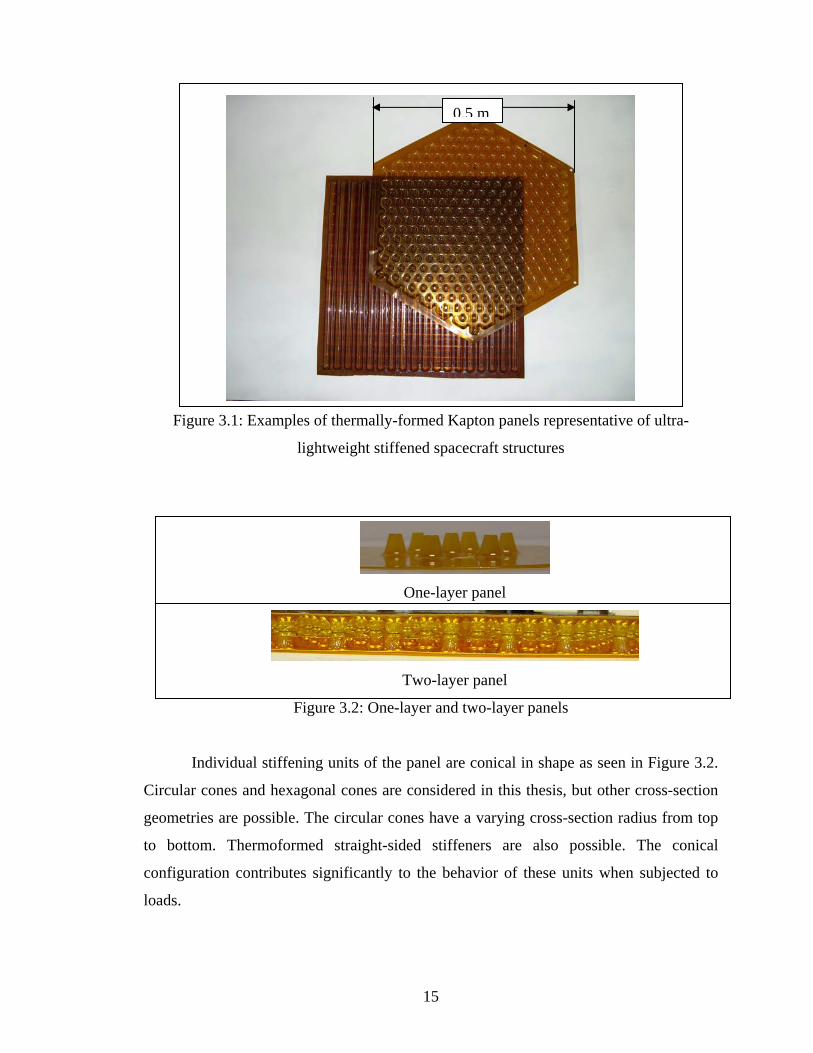
0.5 m

Figure 3.1: Examples of thermally-formed Kapton panels representative of ultra-

lightweight stiffened spacecraft structures

One-layer panel

Two-layer panel

Figure 3.2: One-layer and two-layer panels

Individual stiffening units of the panel are conical in shape as seen in Figure 3.2.

Circular cones and hexagonal cones are considered in this thesis, but other cross-section

geometries are possible. The circular cones have a varying cross-section radius from top

to bottom. Thermoformed straight-sided stiffeners are also possible. The conical

configuration contributes significantly to the behavior of these units when subjected to

loads.

15

The two-layer panel tested for this thesis consists of the two cones that are bonded

to each other (as presented in Figure 3.3) at the contact surface to avoid relative lateral

movement while being loaded.

Two-layer sample

Top cone

Bottom cone

Figure 3.3: Top cone and bottom cone of two-layer panel

Each panel is characterized by several dimensional parameters which are

controlled during the manufacturing process. These parameters are critical to their

performance when subjected to loading. The parameters are illustrated in Figure 3.4 in

which

t is the thickness of the Kapton sheet,

T is the assembled panel thickness,

r is the smallest radius of the cone,

R is the largest radius of the cone,

h is the cone height, and

d is the center-to-center distance between adjacent cones in a layer.

16

Figure 3.4: Dimensional parameters of a panel

d

r

t

h

R

T

17

3.3 Static Experiments of Single-Unit Stiffeners

A series of static experiments were conducted on stiffening units and on panels of

varying configurations. These experiments were aimed mainly at understanding the

stiffness characteristics of the stiffener units and of the assembled panels. Table 3.1

presents the different samples that were tested to develop an understanding of unit

conical stiffener behavior.

Table 3.1: Unit stiffener samples and four-unit sample tested

Sample designation Configuration Dimensions Picture

Sample A1

One-unit, one-

layer panel, top

cone

r= 3.17mm

h=7.93mm

R = 15.87mm

Sample A2

One-unit, one-

layer panel,

bottom cone

r=3.17mm

h=7.93mm

R=15.87mm

Sample B One-unit, two-

layer panel T=15.87mm

Sample C Four-unit, two-

layer panel d=25.4mm

18

The experimental setup for one-unit and four-unit samples consists of a sensitive

weighing scale (Ohaus model EP4102 C) and a precision movable platform (Newport

model 340RC) used to displace the samples. As seen in Figure 3.5, the sample is mounted

securely to the platform and then lowered until it is just in contact with the scale. The

scale is then set to zero and the test is started from this point.

Weighing scale

Sample under test

Slide block (used to apply displacement

R

F

+

Figure 3.5: Experimental schematic and setup for static test of panel units.

19

The loading cycle consisted of a series of precise displacements, first increasing

the vertical force on the sample and then decreasing it. The free body diagram is also

presented in Figure 3.5 with the sign convention for displacement. Displacements in steps

of 0.05mm were used. The corresponding reaction force displayed on the scale was

recorded. The load was then slowly released by reversing the displacement sequence by

raising the slide block in increments of 0.05mm. Again, the corresponding reaction force

was recorded for each step. The force-displacement results were consistent. The results of

this test are presented in Section 3.4 and the test data is presented in Appendix 1.

Figure 3.6 shows the load-displacement plot for a single loading cycle of the one-

unit, one-layer top cone, sample A1. The vertical axis is the force in Newtons. The

horizontal axis is the corresponding displacement in mm. The slope of the curve is

approximately 3 N/mm. The loading and unloading sequences are not identical, forming a

hysteresis loop. Both the loading and unloading cycles show a slight stiffening trend (an

increasing slope with increasing displacement).

0 0.2 0.4 0.6 0.8 1 1.2 1.40

0.5

1

1.5

2

2.5

3

3.5

4

Forc

e (N

)

Displacement (mm)

loading

unloading

Figure 3.6: Force-displacement plot for Sample A1

The load-displacement plot for a single loading cycle of the one-unit, one-layer bottom

cone, sample A2 is presented in Figure 3.7. It should be noted that sample A1 and A2

have the same height. However, in sample A1, the conical area is thinner for greater

sections of the cone compared to sample A2. Here, the loading and unloading results are

20

similar to those of sample A1, also forming a hysteresis loop. The slope of the curve is

approximately 5 N/mm and is about 66% stiffer than the sample A1. Both loading and

unloading cycles show a slight stiffening trend, although less than that seen in sample A1.

0 0.2 0.4 0.6 0.8 1 1.2 1.40

1

2

3

4

5

6

Forc

e (N

)

Displacement (mm)

loading

unloading

Figure 3.7: Force-displacement plot for Sample A2

Following the static test on samples A1 and A2, the one-unit, two-layer sample B

was tested. The same test procedure and test setup as for samples A1 ad A2 were used.

Two sample B units were tested. Results for both are included in Appendix 1. Force-

displacement results for one sample are presented in Figure 3.8. This loading and

unloading sequence was repeated three times. Here, the force-displacement plots indicate

that the slope increases significantly beyond a certain load. For small loads, the

deformation of the top cone appeared to be more prominent. With higher loads, the top

cone had deformed up to a certain point beyond which deformation of the bottom cone

was noticed. The slope of the lower portion of this plot is approximately 1.5 N/mm and

that of the steeper portion of this plot is approximately 3 N/mm compared to the

calculated combined slope of approximately 2 N/mm with top cone and bottom cone

modeled as springs in series.

21

Figure 3.8: Force-displacement plot for sample B1

Figure 3.9 illustrates the progression of local deformations of the two-layer, one-

unit panel (Sample B) unit as observed during the loading cycle. It is described in six-

steps. Step 1 indicates the sample condition at the time of applying the loads. As the load

is applied gradually, the top cone of the sample begins to twist as indicated in step 2. The

top cone twists up to a particular point beyond which further application of load causes

the bottom cone to twist. This process is initiated by signs of buckling of the top cone as

can be seen in step 3. Beyond this point, the bottom cone begins to deform as in step 4.

Further loading causes the two cones to buckle. This sequence of progression is observed

for every load cycle of the samples. The twisting of the cones was more prominent to the

naked eye in the two-layer, one-unit samples.

22

Figure 3.9: Schematic representation of progression of deformation for two-layer, one-

unit sample under loading

Top cone

Bottom cone

Lines indicating twisting

Small groove indicating signs of buckling

Small dimples formed

Small dimples being formed in bottom cone

Dimples lead to buckling

Light buckling noticed on bottom cone

LOADING 1 2 Direction of

twist

3 4

5 6

23

Figure 3.10 presents the force-displacement results for the four-unit-two-layer panel

(Sample C). The stiffness of the lower portion of this plot is approximately 2 N/mm and

the steeper portion of this plot is approximately 10 N/mm compared with the calculated

slope of 7.5 N/mm with four two-layer-one-unit samples in parallel. The transition point

of the curve occurs approximately at 0.25 N. It can be seen that the sharper bilinear

property of the individual units as seen in Figure 3.8 is smoothed for the four-unit-two-

layer sample where four stiffener units are combined together in parallel. The force-

displacement plot of the four-unit-two-layer sample in Figure 3.10 shows a smoother

transition from the lower less-stiff slope to the steeper portion compared to the one-unit-

two-layer stiffeners in which case the transition can be approximated as a bilinear

stiffness. The approximate calculated stiffness of four series springs in parallel is 7.5

N/mm based on the static test experiments on samples A1 and A2.

Figure 3.10: Force-displacement plot for sample C

3.4 Static Experiments of One-Layer Panels

Tests were also performed on a set of one-layer panels. Several one-layer panels

made of circular cone stiffeners (referred to as Samples C1-C4) and hexagonal cone

stiffeners (referred to as Sample H) were tested. Stiffener geometries are seen in Figure

3.11.

24

Figure 3.11: Circular cone and hexagonal cone samples

Four configurations for sample C were tested. The details of the configurations

and dimensional details are presented in Table 3.2. A pictorial comparison of different

configurations of sample C is presented in Figure 3.12.

Table 3.2: Dimensional variations of the one-layer samples

Sample Radius ‘r’ Height ‘h’

C 1 3.175 mm 4.96 mm

C 2 3.175 mm 4.96 mm

C 3 3.175 mm 11.9 mm

C 4 12.7 mm 9.9 mm

H 1 12.7 mm 11.9 mm

H 2 12.7 mm 11.9 mm

25

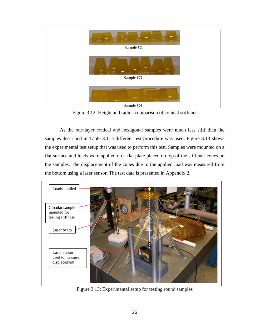
Sample C1

Sample C3

Sample C4

Figure 3.12: Height and radius comparison of conical stiffener

As the one-layer conical and hexagonal samples were much less stiff than the

samples described in Table 3.1, a different test procedure was used. Figure 3.13 shows

the experimental test setup that was used to perform this test. Samples were mounted on a

flat surface and loads were applied on a flat plate placed on top of the stiffener cones on

the samples. The displacement of the cones due to the applied load was measured from

the bottom using a laser sensor. The test data is presented in Appendix 2.

Figure 3.13: Experimental setup for testing round samples

Laser sensor used to measure displacement

Circular sample mounted for testing stiffness

Loads applied

Laser beam

26

Figure 3.14 shows the force-displacement plots for samples C1, C2, C3, C4 and

sample H (refer to table 3.2). The displacements are plotted only for the loading cycle. It

was not possible to record the displacements for the unloading cycle because only very

minor variations were noticed during unloading and the experimental setup was not

accurate to capture these small variations. The loads were applied using 20g, 50g, 100g,

and 200g masses respectively. As it was difficult to get accurate results for each load, the

tests were repeated three times. As only three displacements were recorded for each data

set, the plots in Figure 3.13 are the curve fit for the data points recorded. Samples C1 and

C2 are plotted together and samples H1 and H2 are plotted together. Based on the results

seen, the test procedure adopted to test these samples was questioned and also, varying

bilinear trends were seen. More study with a different experimental procedure is

recommended for these samples.

0

0.5

1

1.5

2

2.5

0 0.1 0.2 0.3 0.4

Displacement (mm)

Forc

e (N

)

C1C2

C3

0

0.1

0.2

0.3

0.4

0.5

0.6

0 0.05 0.1 0.15 0.2 0.25 0.3

Displacement (mm)

Forc

e (N

)

C3

Sample C 1 and C2 Sample C 3

C4

0

2

4

6

8

10

12

0 0.02 0.04 0.06 0.08 0.1 0.12

Displacement (mm)

Forc

e (N

)

C4

0

0.5

1

1.5

2

2.5

0 0.1 0.2 0.3 0.4 0.5 0.6

Displacement (mm)

Forc

e (N

)

H1H2

Sample C 4 Sample H 1 and H2

Figure 3.14: Force-displacement plots for samples C1, C2, C3, C4, H1 and H2

27

3.5 Static Experiments of Two-Layer Full Panel

A different test procedure was adopted for performing the static test on the full

panel. The panel was mounted in such a way to approximate a standard beam bending

test with simply supported boundary condition on two sides using circular supports.

Double-sided tapes lightly secured the panel to the supports to ensure that it did not lose

contact with the surface while applying loads. This is presented in Figure 3.15.

132 mm

Point B

Point A

Mid point (where load was applied)

Figure 3.15: Panel setup for static test

The center of the panel was located and static loads were applied at this point.

Laboratory hanging masses were used to apply the load from 0.0981 N (10 g mass)

through 0.981 N (100g mass) in increments of 0.0981 N. Two points A and B were

located 132 mm from the center as shown in figure 3.14. The vertical displacement of A

was measured for each load step with a laser sensor. The laser sensor was mounted above

the panel and adjusted so that the beam was focused on point A. The same was repeated

for point B. A computer based data acquisition system was used to record the output of

the laser sensor. Figure 3.15 presents the entire setup that was used to perform this test.

28

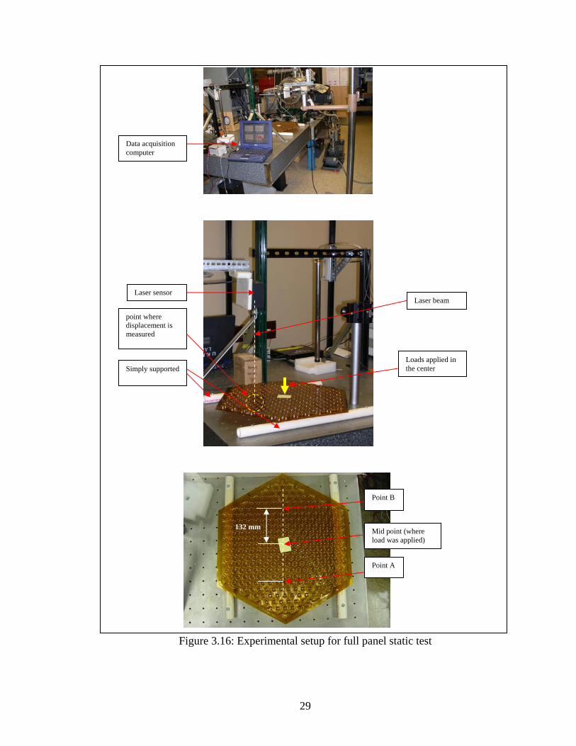
Figure 3.16: Experimental setup for full panel static test

Data acquisition computer

Laser sensor

Simply supported

point where displacement is measured

Loads applied in the center

Laser beam

132 mm

Point B

Point A

Mid point (where load was applied)

29

As can be seen in Figure 3.16, the panel was supported on two sides on the

stiffener units and not on the flanges. This was done because the bending property of the

panel was the main focus of the experiment and not the flange bending properties.

The maximum loading range was limited to 0.981 N for this test. For higher loads

(1.2 N and higher), a distinct click sound was heard from the panel stiffener units

indicating local buckling of the stiffener units. The test was repeated three times for each

point with no appreciable difference in results.

The force-displacement plots for the panel are presented in Figure 3.17 and all the

test data is presented in Appendix 3. Plots of the data for both points are compared in

Figure 3.17. It can be seen that at Point A, the panel behaved approximately linearly over

the entire range of loading. However at Point B, the panel tends to soften approximately

after a load of 0.6 N.

0

0.1

0.2

0.3

0.4

0.5

0.6

0.7

0.8

0.9

1

0 0.002 0.004 0.006 0.008 0.01 0.012 0.014

Deflection (mm)

Forc

e (N

)

pt Apt B

Figure 3.17: Force-displacement plots for points A and B for full panel

30

3.6 Results Summary

The force-displacement plots in Figures 3.6 and 3.7 indicate that the single layer

conical stiffener units exhibit approximately linear stiffness. However, Figure 3.8 shows

that the two-layer stiffener unit exhibits hardening characteristics that can be

approximated as a bilinear static response. This, combined with the qualitative

observation of deformation of the stiffener unit suggests that they could be modeled using

spring elements, either a single spring with experimental force-displacement

characteristics of the two-layer stiffener unit or two springs in series with experimental

force-displacement characteristics of the individual single layer conical stiffener units. It

is also seen from Figure 3.8 that the stiffness of the two layer stiffener unit in the steeper

part of the curve is higher than the calculated stiffness using the top and bottom cone in

series. A similar behavior is seen in Figure 3.10 where the stiffness of the four-unit panel

is about 20% more than the calculated value.

Further, the plots in Figure 3.17 indicate that the panel behaves approximately

linearly over the entire load range for both points tested. Apparently, the bilinear

behavior of the individual stiffener units is diminished when a number of individual units

act in parallel. Details of the finite element modeling process and the comparison of the

model behavior with the tested sample behavior, along with further discussion of the

nonlinear characteristics of the structure, are presented in Chapter 4.

31

CHAPTER FOUR

Finite Element Modeling

4.1 Introduction

This chapter presents a description of the process of developing finite element

(FE) models of the panel units discussed in the previous chapter. It presents the approach

used to arrive at a FE model for the complete panel. Sections of this chapter present the

types of elements used for the model and their characteristics. The boundary conditions

and the type of loading applied to the model are also discussed. Finally, the results of the

static analysis performed on the FE model of the two-layer panel are presented.

4.2 Finite Element Modeling

As seen in the previous chapter, the stiffening units display nonlinear

characteristics when subjected to loading. One approach to modeling these stiffeners

would be to develop detailed models including material complexities and other intricate

details. However, this could lead to a model with too many dofs to be useful for design.

The second approach would be to model the stiffeners as nonlinear spring elements. This

approach would be a more practical and simplistic approach.

The second approach was chosen to develop finite element models of the

individual stiffener units. Based on this approach, the panels units are modeled as

nonlinear springs with either two or three nodes. The outer-surface Kapton sheets

connecting the stiffener units are modeled as shell elements with corner nodes. The

thinner sheet of Kapton present in between the two cones in the tested sample (refer to

Figure 3.3) is not represented in the corresponding FE model as its primary purpose is to

provide a surface for bonding the two cones together. The full panel does not include this

thin intermediate sheet. A detailed description of the panel modeling based on this

approach is presented in the following sections.

32

4.3 Modeling Individual Stiffener Units

Based on the static displacement experiments that were conducted on different

sets of individual stiffener elements described in Chapter 3, two FE models were

developed to represent the panel stiffener units. Two approaches were considered for

modeling the stiffener elements: 1) Model 1 was to model the top and bottom cones using

different nonlinear spring elements and then use a serial combination of these springs to

represent the two-layer, one-unit stiffener and 2) Model 2 was to model the two-layer,

one-unit stiffener as a single nonlinear spring.

4.3.1 Description of Two-Spring and One-Spring Models of Stiffener Unit

Figure 4.1 presents a representation of the two-spring and the one-spring models.

A pictorial representation of stiffener unit is also presented. The two-spring model has

three nodes and the one-spring model has two nodes. The FE model of the two-layer,

one-unit stiffener using Model 1 is presented in Figure 4.2 and the FE model using

Model 2 is presented in Figure 4.3.

Model 1 Model 2 Two-spring model One-spring model

Bottom cone (Larger)Middle thinner

Kapton sheet

Top cone

2

1

3

2

1

Figure 4.1: Two-spring model (left) and one-spring model (right) of two-layer, one-unit stiffener

33

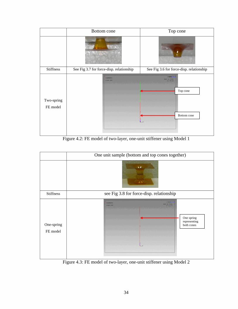
Bottom cone Top cone

Stiffness See Fig 3.7 for force-disp. relationship See Fig 3.6 for force-disp. relationship

Two-spring

FE model

Top cone

Bottom cone

Figure 4.2: FE model of two-layer, one-unit stiffener using Model 1

One unit sample (bottom and top cones together)

Stiffness see Fig 3.8 for force-disp. relationship

One-spring

FE model

One spring representing both cones

Figure 4.3: FE model of two-layer, one-unit stiffener using Model 2

34

The ANSYS version 8.0 nonlinear spring element (COMBIN39) was used to

model the individual panel units. COMBIN39 is a unidirectional element with nonlinear

generalized force-deflection capability that can be used in any analysis. The element has

longitudinal or torsional capability in 1-D, 2-D, or 3-D applications. The element has one

dof at each node in the axial direction. Experimental results obtained from static

deflection tests performed on different sets of individual stiffener units were used to

define the element properties in the axial direction. Refer to Section 3.4.1 for details of

how the spring properties were measured.

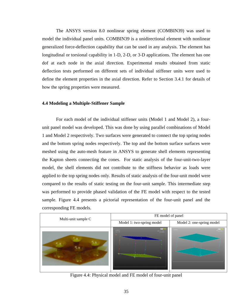
4.4 Modeling a Multiple-Stiffener Sample

For each model of the individual stiffener units (Model 1 and Model 2), a four-

unit panel model was developed. This was done by using parallel combinations of Model

1 and Model 2 respectively. Two surfaces were generated to connect the top spring nodes

and the bottom spring nodes respectively. The top and the bottom surface surfaces were

meshed using the auto-mesh feature in ANSYS to generate shell elements representing

the Kapton sheets connecting the cones. For static analysis of the four-unit-two-layer

model, the shell elements did not contribute to the stiffness behavior as loads were

applied to the top spring nodes only. Results of static analysis of the four-unit model were

compared to the results of static testing on the four-unit sample. This intermediate step

was performed to provide phased validation of the FE model with respect to the tested

sample. Figure 4.4 presents a pictorial representation of the four-unit panel and the

corresponding FE models. FE model of panel

Multi-unit sample C Model 1: two-spring model Model 2: one-spring model

Figure 4.4: Physical model and FE model of four-unit panel

35

In addition to the spring elements in Section 4.3.1, the model includes shell elements

(SHELL 63) for the top and bottom layers of the multi-unit sample. SHELL 63 has both

bending and membrane capabilities. The element has six degrees of freedom at each

node. A thickness of 0.127 mm (5 mil) was used for the shell elements composing the top

and bottom Kapton layers of the sample. This was obtained by measuring the thickness of

the Kapton sheet in the tested sample. Table 4.1 lists the physical properties of Kapton

that were used for the model.

Table 4.1: Physical properties of Kapton Property Value

Tensile Modulus 2.5 G Pa

Poisson’s ratio 0.34

Density 1.42 E3 Kg/m³

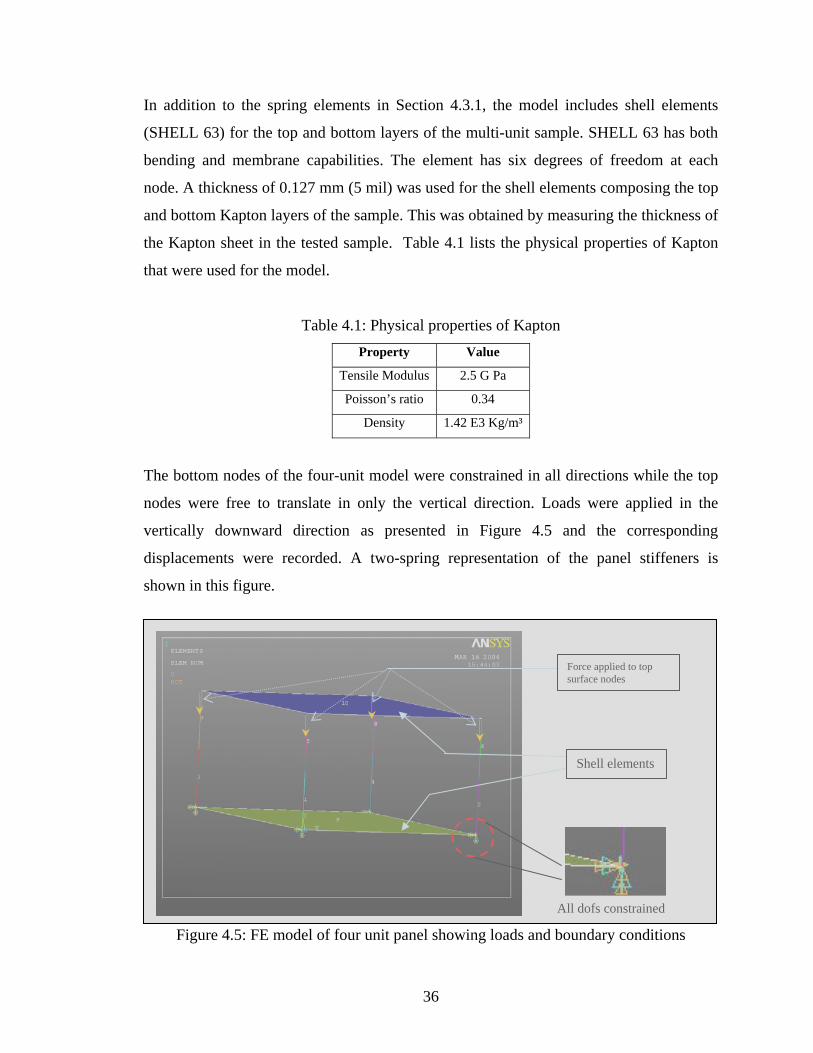
The bottom nodes of the four-unit model were constrained in all directions while the top

nodes were free to translate in only the vertical direction. Loads were applied in the

vertically downward direction as presented in Figure 4.5 and the corresponding

displacements were recorded. A two-spring representation of the panel stiffeners is

shown in this figure.

Figure 4.5: FE model of four unit panel showing loads and boundary conditions

All dofs constrained

Shell elements

Force applied to top surface nodes

36

Figure 4.6 shows the results of the static analysis with the four-unit models using

a two-spring stiffener (Model 1) and a one-spring stiffener (Model 2) plotted with the

static test results. The displacement in mm is plotted in the horizontal axis and the force

in Newtons is plotted in the vertical axis. From Figure 4.6 it can be seen that the results of

FE Model 2 show more pronounced nonlinear behavior in the region from 0 to 0.2 mm

displacement than FE Model 1. FE Model 2 has a distinctly changing slope from a

stiffness less than that of FE Model 1 to a stiffness approximately 33% greater than that

of FE Model 1. The experimental results also exhibit a distinct change in slope, but in the

region 0 to 0.4 mm displacement. The results of FE Model 1 exhibit a less-changing

slope, with the final stiffness more parallel to the experimental result.

Figure 4.6: FE model results compared to static test results for four-unit panel.

The stiffness of the lower portion of the experimental results plot in Figure 4.6 is

approximately 2 N/mm and the steeper portion of this plot is approximately 10 N/mm

compared with slopes of 1.5 N/mm and 3 N/mm of the one-unit stiffener in Figure 3.8

respectively. In parallel, the stiffness of the four-unit panel should be about 4 times the

stiffness of one-unit stiffener. From the results of the static experiment performed on the

four-unit test sample, it is noted that the structure stiffens beyond a certain load. A similar

37

behavior is also seen in the FE results of Model 2 (one-spring model). To include this

nonlinear behavior, Model 2 was selected for use in the full-panel FE model. Additional

efforts are needed to better correlate the four-unit models to the experimental results.

4.5 Modeling the Complete Panel

Based on the observation from the four-unit sample model, the complete panel was

modeled using multiple one-spring stiffener units spaced in a hexagonal honeycomb-

pattern. Figure 4.7 shows the FE model of the full panel. The nonlinear spring elements

and the shell elements used to connect them are highlighted. The FE model is comprised

of 241 spring elements and 10,801 shell elements. The batch file (ANSYS data input file)

used to create the model of the full panel is presented in Appendix 5. The flanges of the

panel were not included in the model at first, as the bending characteristics of the flanges

was thought not to be of interest. The nodes on two parallel edges 1 and 2 of the lower

surface were constrained in translation. Loads were applied to the center node of the top

surface and the vertical deflection of the nodes corresponding to points A and B in the

actual panel (see Figure 3.15) were recorded.

Shell element

Edge 1 (bottom surface)

Edge 2

Nonlinear spring elements

Figure 4.7: FE model of complete panel using one-spring model

(Model 2) for each stiffener unit

38

The results of the static analysis on the full panel are presented in Figure 4.8 in

comparison with the results of the static experiment. The data for the static analysis on

the full panel is presented in Appendix 6. The deflection in mm is plotted on the

horizontal axis and the force in Newtons is plotted on the vertical axis. The plot indicates

that the FE model results and the test results follow a linear trend. The FE model was

considered a sufficiently accurate representation of the full panel in static

analysis to continue to the dynamic analysis effort.

The nonlinearly increasing stiffness observed from the data of the four unit panel

model seems to have diminished significantly in the full panel model and in the full panel

experiment. However, the test results still show a slight softening trend of the panel as the

load increases. From these results it is theorized that in thermoform-stiffened panel

structures the effect of nonlinearities localized in individual stiffeners is diminished when

many such stiffeners combine to form the complete panel.

0.0000

0.2000

0.4000

0.6000

0.8000

1.0000

1.2000

0.0000 0.0020 0.0040 0.0060 0.0080 0.0100

Defelction (mm)

Forc

e (N

) FEA

test pt Btest pt A

Figure 4.8: Comparison of FE Analysis and experimental results for static analysis on full

panel

39

Dynamic testing was performed to further compare the behavior of the model

when subjected to dynamic loads. The following chapter describes the details of dynamic

testing and dynamic analysis performed on the complete model.

40

CHAPTER FIVE

Dynamic Experimentation and Modeling

5.1 Introduction

This chapter presents the details of modal testing that was performed on the panel.

The experimental setup and test procedure are explained in detail. The second part of this

chapter includes details of the finite element modal analysis that was performed with

several full panel models. Plots for different mode shapes are presented. The results of

the physical testing and the FE model analysis are then compared.

5.2 Modal Tests on Full Panel

Modal testing was performed on the panel using standard modal testing practices as

possible, with modifications as needed. Figure 5.1 shows the test setup that was used to

perform the modal testing. The panel was suspended by two mono-filament lines, each

400 mm long. This was to approximate free-free boundary conditions and to minimize

the effect of rigid body modes on the elastic mode response between 0-100 Hz.

Figure 5.1: Modal testing setup

Figure 5.1: Test setup for panel modal testing

Mono-filament lines

Panel Table

Signal conditioner

Impact hammer

Accelerometers Zodiac computer based data acquisition system

41

A conventional single point impact hammer (PCB 086B01) was modified by

attaching a rectangular aluminum plate measuring 38.1 mm in width and 101.6 mm in

length to its tip in order to mitigate local deformation on the panel at the point of impact.

Griffith recognized the effect of local deformation when testing an inflatable torus with

impact hammer excitation and used a similar modification for his hammer input [14].

Figure 5.2 shows the impact hammer and plate used to excite the panel for modal testing.

Figure 5.2: Impact hammer and aluminum plate

The vibration response of the panel was measured at 24 different points using a 2-

g small-mass accelerometer (PCB Model A353A16) with a nominal voltage sensitivity of

10mV/g and a frequency range between 1 – 10,000 Hz. A second accelerometer was used

as a reference. The reference accelerometer was located in the center of the panel behind

the point where excitation impact was applied. The location of the response

accelerometer was changed to different predefined points during the course of testing to

be able to compute the frequency response for different points on the panel. Figure 5.3

shows the location of the predefined points numbered in the clockwise direction starting

from the inner blue points to the outer red points.

42

Figure 5.3: Pre-defined accelerometer locations

The input force time history data from the impact hammer and the output response time

history from the accelerometer were recorded by a multi-channel mobile dynamic signal

analyzer. A sampling rate of 200 samples per second was used. Preliminary testing

showed that five averages were sufficient for this test. The frequency response functions

were determined at 24 points using by the single-input single-output (SISO) method. The

panel was excited in the center for each test and the response was measured at points 1

through 24 in turn. For each location of the response accelerometer, the panel was excited

five times and the average of the five readings was recorded as the final FRF. Averaging

reduces the noise producing a more accurate FRF. FRF plots for response measured at 13

points are presented in Appendix 7. Figure 5.4 presents the FRF plots for location points

1, 3, 12 and 14.

43

Figure 5.4: Typical better FRF for locations 1, 3, 12 and 14

Frequency in Hertz is plotted on the horizontal axis and amplitude in G^2/Hz is plotted

on the vertical axis. Significant peaks are highlighted in the figure with dotted lines to

show the comparison. The first peak in each plot is expected to be the pendulum mode of

the panel swinging on the monofilament lines. This frequency was estimated using the

panel dimension of 0.250 m from the top edge to the center and compared to the

measured values in the FRFs. Table 5.1 presents the calculated and measured values of

natural frequency for the pendulum mode.

Table 5.1: Comparison of natural frequency for pendulum mode

Measured natural frequency in pendulum mode Calculated natural frequency

in pendulum mode Point 1 Point 3 Point 7 Point 12

0.63 Hz 1.4 Hz 1.5 Hz 1.4 Hz 1.4 Hz

44

After the pendulum mode, the next peaks seen in the FRFs are approximately at

12-12.5 Hz, 21-23 Hz, 29-35 Hz and 39-40 Hz respectively. Figure 5.5 presents two

examples of low-quality FRF plots that were also recorded during the test. In these plots

and others like them the averaged FRF does not show clear peaks typical of modal

response.

Figure 5.5: Bad FRF plots

Measured frequency response function data can be loaded into X-Modal software

(modal analysis software) which can be used to identify modal quantities including

natural frequencies, mode shapes and damping. The frequencies and mode shapes

identified using X-Modal can be compared to those obtained from the modal analysis of

the finite element model. However, the results of X-modal analysis are not available as

this part of the original thesis plan was not completed. Another, less accurate method to

compare the experimental response to that of the finite element model is to compare

45

natural frequencies. However, without mode shapes to compare, frequency matching is

uncertain.

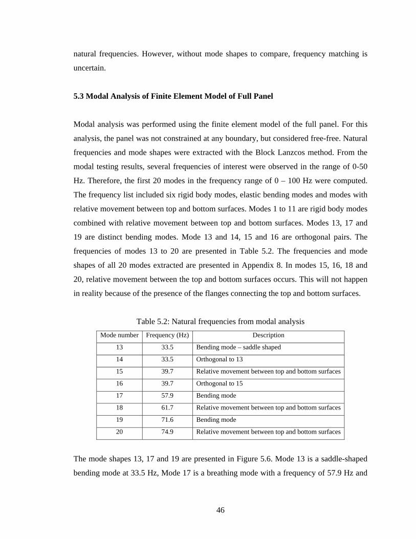
5.3 Modal Analysis of Finite Element Model of Full Panel

Modal analysis was performed using the finite element model of the full panel. For this

analysis, the panel was not constrained at any boundary, but considered free-free. Natural

frequencies and mode shapes were extracted with the Block Lanzcos method. From the

modal testing results, several frequencies of interest were observed in the range of 0-50

Hz. Therefore, the first 20 modes in the frequency range of 0 – 100 Hz were computed.

The frequency list included six rigid body modes, elastic bending modes and modes with

relative movement between top and bottom surfaces. Modes 1 to 11 are rigid body modes

combined with relative movement between top and bottom surfaces. Modes 13, 17 and

19 are distinct bending modes. Mode 13 and 14, 15 and 16 are orthogonal pairs. The

frequencies of modes 13 to 20 are presented in Table 5.2. The frequencies and mode

shapes of all 20 modes extracted are presented in Appendix 8. In modes 15, 16, 18 and

20, relative movement between the top and bottom surfaces occurs. This will not happen

in reality because of the presence of the flanges connecting the top and bottom surfaces.

Table 5.2: Natural frequencies from modal analysis Mode number Frequency (Hz) Description

13 33.5 Bending mode – saddle shaped

14 33.5 Orthogonal to 13

15 39.7 Relative movement between top and bottom surfaces

16 39.7 Orthogonal to 15

17 57.9 Bending mode

18 61.7 Relative movement between top and bottom surfaces

19 71.6 Bending mode

20 74.9 Relative movement between top and bottom surfaces

The mode shapes 13, 17 and 19 are presented in Figure 5.6. Mode 13 is a saddle-shaped

bending mode at 33.5 Hz, Mode 17 is a breathing mode with a frequency of 57.9 Hz and

46

Mode 19 is another bending mode at 71.6 Hz. Modes 10, 11 and 18 are presented in

Figure 5.7. In these modes, relative movement between the top and bottom surfaces

occurs.

MODE 19 – 71.6 Hz

MODE 17 – 57.9 Hz MODE 13 – 33.5 Hz

Figure 5.6: Mode shapes 13, 17 and 19

47

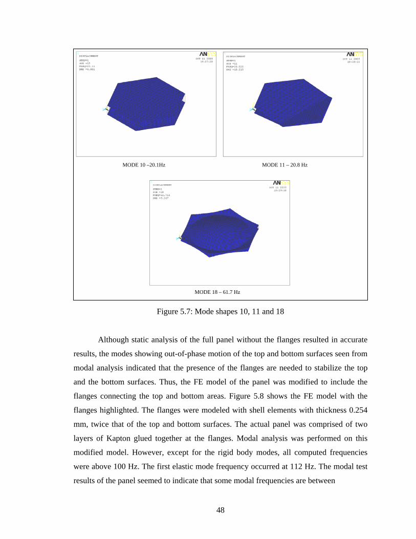
MODE 10 –20.1Hz MODE 11 – 20.8 Hz

MODE 18 – 61.7 Hz

Figure 5.7: Mode shapes 10, 11 and 18

Although static analysis of the full panel without the flanges resulted in accurate

results, the modes showing out-of-phase motion of the top and bottom surfaces seen from

modal analysis indicated that the presence of the flanges are needed to stabilize the top

and the bottom surfaces. Thus, the FE model of the panel was modified to include the

flanges connecting the top and bottom areas. Figure 5.8 shows the FE model with the

flanges highlighted. The flanges were modeled with shell elements with thickness 0.254

mm, twice that of the top and bottom surfaces. The actual panel was comprised of two

layers of Kapton glued together at the flanges. Modal analysis was performed on this

modified model. However, except for the rigid body modes, all computed frequencies

were above 100 Hz. The first elastic mode frequency occurred at 112 Hz. The modal test

results of the panel seemed to indicate that some modal frequencies are between

48

0-100 Hz. The addition of the flanges to the FE model made it much stiffer than the

actual panel. Since the frequencies of the panel model with the flanges were much higher

than the actual frequencies, the flanges were not included.

FLANGE

FLANGE

Figure 5.8: FE model of panel with flange

Another approach was tried to avoid the relative out-of-phase motion between the

top and bottom surfaces. Springs with high stiffness (500 times the actual model spring,

2500 N/mm) were used to connect the top and bottom surfaces at the six corner nodes.

This was done so that the top and bottom surfaces of the panel would move together.

However, because the spring lacked stiffness in the lateral directions, this approach did

not prevent all out-of-phase motions between the top and bottom areas.

49

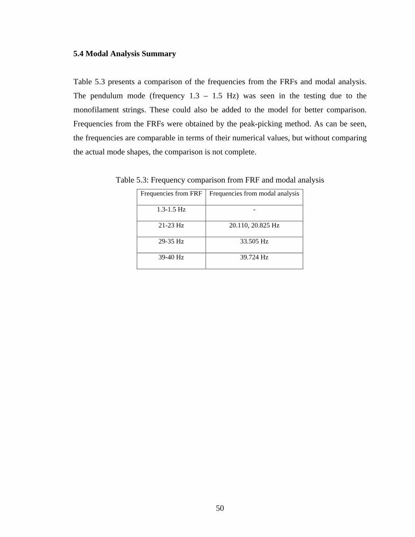
5.4 Modal Analysis Summary

Table 5.3 presents a comparison of the frequencies from the FRFs and modal analysis.

The pendulum mode (frequency 1.3 – 1.5 Hz) was seen in the testing due to the

monofilament strings. These could also be added to the model for better comparison.

Frequencies from the FRFs were obtained by the peak-picking method. As can be seen,

the frequencies are comparable in terms of their numerical values, but without comparing

the actual mode shapes, the comparison is not complete.

Table 5.3: Frequency comparison from FRF and modal analysis Frequencies from FRF Frequencies from modal analysis

1.3-1.5 Hz -

21-23 Hz 20.110, 20.825 Hz

29-35 Hz 33.505 Hz

39-40 Hz 39.724 Hz

50

CHAPTER SIX

Thesis Summary

6.1 Summary and Conclusions

This chapter presents a comprehensive summary of this thesis. Recommendations

for future work in the area of thermoformed stiffened panel structures are also included.

The main objective of this thesis was to develop an understanding of the behavior of a

thermoformed stiffened panel and to develop a finite element model of the panel based on

static experimentation. The evaluation of the dynamic behavior of the panel was also of

interest.

First, the smallest stiffener unit was tested. Static tests were performed and unit

stiffness properties were established. Static tests were performed on each cone element of

the unit stiffener to understand their individual properties and on the combined stiffener

consisting of two cones. During the course of static testing, the mechanisms of

deformation were also studied, providing a better understanding of the deformation

phenomenon. Although each of the two cones behaves linearly in static tests of their

stiffness under axial loading, the combination of these cones in a unit stiffener was seen

to have a bi-linear stiffness. However, from the static test on a four-unit panel it was seen

that bi-linear behavior diminishes when multiple unit stiffeners were combined. Both,

hexagonal and circular configurations of the stiffener cone elements were tested.

Based on the results of static tests, two FE models were developed for the

stiffener units using nonlinear springs; 1) one-spring model, 2) two-spring model. In the

one-spring model, the stiffener unit was modeled as a single spring and in the two-spring

model, two springs were used each representing the individual cones of the stiffener unit.

A four-unit stiffener was modeled using the two modeling approaches. The analysis

results of this model were compared with test results obtained by testing a four-unit panel

51

to find that the one-spring unit model produced a result with better qualitative correlation

to test results. Neither model provided good qualitative correlation.

Based on this comparison, a full-panel model was developed using the one-spring

model for each stiffener unit. Static tests were performed on the full panel and static

analysis was done on the FE model of the full panel. The results of these tests and

analysis were compared to find that the full panel model produced a result qualitatively

and quantitatively comparable to the test results.

Modal testing was performed on the full panel and frequency response functions

were determined. The frequencies of the analysis and the frequencies from frequency

response function (obtained by peak picking) were compared. Modal testing revealed

bending modes between frequencies 0-100 Hz.

Modal analysis was performed on the FE model and mode shapes and natural

frequencies were extracted. Based on the analysis, the FE model was modified to include

the side flanges connecting the two layers of the panel and this resulted in higher stiffness

of the panel than indicated by the experimental results.

6.2 Conclusions

Although this thesis demonstrates that conventional testing principles could be

applied to testing thermoformed stiffener panels. The phased-verification approach used

in this thesis - where the full panel was broken down into smaller units and properties

were established for these smaller units and then used to develop FE models for the full

panel – can be extended to modeling and testing similar structures. The concept of using

nonlinear springs to represent stiffener units for thermoformed stiffening units has been

established during the course of this work. This reduces the need for in-depth modeling

of similar structures thus making the idea of modeling extremely large structures feasible

due to the limited number of nodes needed for such models compared to complicated

models. This concept can be applied to similar stiffening structures.

52

6.3 Recommendations for Future Work

There are five main recommendations for future work related to thermoformed

stiffener panels similar in construction to the panel discussed in this thesis.

First, a selection of stiffener units needs to be tested to document the range of

behavior more completely. Further, the unit stiffeners should be tested with shear and

torsional loading as well as axial loading as was done herein.

Second, a better way to represent the effect of the flanges connecting the top and

bottom surfaces on the stiffness of the panel needs to be developed. The addition of the

flange would stabilize the top and bottom surfaces and would eliminate the relative

movement between them.

Third, the lateral stiffness of the panel needs to be measured by testing and this

can be used to define lateral spring stiffness in the FE model. Lateral stiffness of the

springs would add constraints on the movement of the spring nodes in the lateral

direction.

Fourth, the damping characteristics of the panel need to be analyzed and

measured. During this thesis, the damping properties of the panel were not measured.

They were not accounted for in the finite element model. The effect of damping will

affect the dynamic characteristics of the panel significantly.

Fifth, future testing of similar thermoform-stiffened ultra-lightweight panels

should include static test on multiple-stiffener sample followed by static testing of

individual stiffener unit cut from the multi-stiffener unit tested. Then the stiffener cones

of the single-stiffener unit sample tested should be taken apart and tested separately. The

results of these tests must then be compared. With this process, the elements comprising

the tested assembly will be tested, rather than assuming similarity of unit stiffeners

throughout.

53

APPENDIX 1

1. Force-displacement results for sample A1 (Fig. 3.6 a)

Force (N) Displacement

(mm) Loading cycle

Unloading cycle

0.0000 0.0000 0.0000 0.0500 0.1711 0.0164 0.1000 0.3273 0.1023 0.1500 0.4978 0.2380 0.2000 0.6856 0.3849 0.2500 0.8682 0.5385 0.3000 1.0553 0.6804 0.3500 1.2558 0.8478 0.4000 1.4539 1.0176 0.4500 1.6563 1.2090 0.5000 1.8433 1.3711 0.5500 2.0470 1.5731 0.6000 2.2615 1.7791 0.6500 2.4834 2.0077 0.7000 2.6920 2.2201 0.7500 2.8990 2.4450 0.8000 3.0886 2.6742 0.8500 3.3003 2.9028 0.9000 3.4824 3.1463 0.9500 3.6715 3.3835 1.0000 3.8682 3.6399 1.0500 3.9091 3.9091

54

2. Force-displacement results for sample A2 (Fig. 3.6 b)

Force (N) Displacement (mm) Loading

cycle Unloading

cycle 0.0000 0.0000 0.0000 0.0500 0.2673 0.0314 0.1000 0.5246 0.2192 0.1500 0.7774 0.4496 0.2000 1.0468 0.6768 0.2500 1.3191 0.8916 0.3000 1.5970 1.1220 0.3500 1.8816 1.3988 0.4000 2.1670 1.6666 0.4500 2.4396 1.9286 0.5000 2.6907 2.2261 0.5500 2.9244 2.4753 0.6000 3.1798 2.7626 0.6500 3.4357 3.0391 0.7000 3.6801 3.3252 0.7500 4.0009 3.6021 0.8000 4.2626 3.9200 0.8500 4.5182 4.2213 0.9000 4.8067 4.4846 0.9500 5.0640 4.8289 1.0000 5.2881 5.1308 1.0500 5.5272 5.5156

55

3. Force-displacement results for sample B (Fig. 3.7)

Sample B 1 Sample B 2 Force (N) Force (N) Displacement

(mm) Loading cycle

Unloading cycle

Loading cycle

Unloading cycle

0 0.0012 0.0000 0.0000 0.0000 0.05 0.0841 0.0000 0.0688 0.0000 0.1 0.1664 0.0368 0.1787 0.0032

0.15 0.2744 0.0867 0.2909 0.0674 0.2 0.3925 0.1589 0.4290 0.1490

0.25 0.5289 0.2592 0.5929 0.2511 0.3 0.6793 0.4034 0.7676 0.3857

0.35 0.8491 0.5532 0.9347 0.5397 0.4 1.0379 0.7151 1.1082 0.6449

0.45 1.2173 0.8579 1.2883 0.7794 0.5 1.3921 1.0287 1.4744 0.9261

0.55 1.5810 1.2091 1.5953 1.0422 0.6 1.7688 1.4116 1.7795 1.1339

0.65 1.9622 1.5661 1.9817 1.2708 0.7 2.1545 1.7657 2.1474 1.4022

0.75 2.3109 1.9639 2.2949 1.5217 0.8 2.4808 2.1650 2.4283 1.6618

0.85 2.6482 2.3915 2.5387 1.7653 0.9 2.8326 2.5794 2.6527 1.8937

0.95 3.0012 2.7907 2.6907 2.0169 1 3.1330 3.0199 2.7036 2.1572

1.05 3.2511 3.2428 2.7718 2.3123

56

4. Force-displacement results for sample C (Fig. 3.8)

Force (N) Displacement (mm) Loading

cycle Unloading

cycle 0.0000 0.0000 0.0000 0.0500 0.0767 0.0000 0.1000 0.1745 0.0000 0.1500 0.3244 0.0362 0.2000 0.5213 0.1289 0.2500 0.7598 0.2896 0.3000 1.0353 0.4740 0.3500 1.3073 0.7204 0.4000 1.6243 0.9616 0.4500 1.9293 1.1982 0.5000 2.2047 1.4997 0.5500 2.4939 1.8217 0.6000 2.7780 2.1598 0.6500 3.0812 2.5226 0.7000 3.4729 2.9376 0.7500 3.7960 3.3410 0.8000 4.1718 3.7679 0.8500 4.5669 4.2128 0.9000 4.9553 4.6845 0.9500 5.3797 5.1470 1.0000 5.8022 5.6197 1.0500 6.2082 6.2003

57

APPENDIX 2

1. Force-displacement results for sample C1 (Fig. 3.13)

Displacement

(mm) Force

(N) 0.02 0.1962 0.245 0.981 0.38 1.962

2. Force-displacement results for sample C2

Displacement (mm)

Force (N)

0.14 0.1962 0.21 0.981 0.25 1.962

3. Force-displacement results for sample C3

Displacement (mm)

Force (N)

0.055 0.1962 0.285 0.4905

4. Force-displacement results for sample C4

Displacement (mm)

Force (N)

0 0.1962 0.08 4.905 0.11 9.81

5. Force-displacement results for sample H1

Displacement (mm)

Force (N)

0 0.1962 0.13 0.4905 0.53 1.962

58

6. Force-displacement results for sample H2

Displacement (mm)

Force (N)

0.125 0.1962 0.131 0.4905 0.525 1.962

59

APPENDIX 3

1. Force-displacement results for full panel at point A (Fig. 3.16)

Displacement (mm) Force (N) Trial 1 Trial 2 Trial 3 0 0.0000 0.0000 0.0000

0.0981 0.0015 0.0010 0.0010 0.1962 0.0027 0.0018 0.0022 0.2943 0.0038 0.0028 0.0030 0.3924 0.0052 0.0041 0.0044 0.4905 0.0068 0.0051 0.0056 0.5886 0.0082 0.0065 0.0071 0.6867 0.0093 0.0077 0.0083 0.7848 0.0108 0.0092 0.0099 0.8829 0.0119 0.0104 0.0109 0.981 0.0132 0.0118 0.0122

2. Force-displacement results for full panel at point B

Displacement (mm) Force

(N) Trial 1 Trial 2 Trial 3 0 0.0000 0.0000 0.0000

0.0981 0.0009 0.0009 0.0011 0.1962 0.0022 0.0021 0.0010 0.2943 0.0032 0.0032 0.0019 0.3924 0.0044 0.0043 0.0030 0.4905 0.0055 0.0054 0.0041 0.5886 0.0067 0.0055 0.0055 0.6867 0.0077 0.0073 0.0065 0.7848 0.0094 0.0088 0.0075 0.8829 0.0101 0.0103 0.0087 0.981 0.0112 0.0114 0.0097

60

APPENDIX 4

1. Force-displacement analysis results for model 1 four-unit test panel (Fig. 4.6)

Force (N)

Displacement (mm)

0 0 0.0767 0.0166 0.3244 0.0704 0.7598 0.1488 1.3073 0.2264 1.9293 0.307 2.4939 0.3782 3.0812 0.4519 3.7960 0.5399 4.5669 0.6315 5.3797 0.7248

2. Force-displacement analysis results for model 2 four-unit test panel

Force (N)

Displacement (mm)

0 0 0.0767 0.0281 0.3244 0.0913 0.7598 0.1549 1.3073 0.2142 1.9293 0.2694 2.4939 0.3145 3.0812 0.3618 3.7960 0.423 4.5669 0.4823 5.3797 0.5594

61

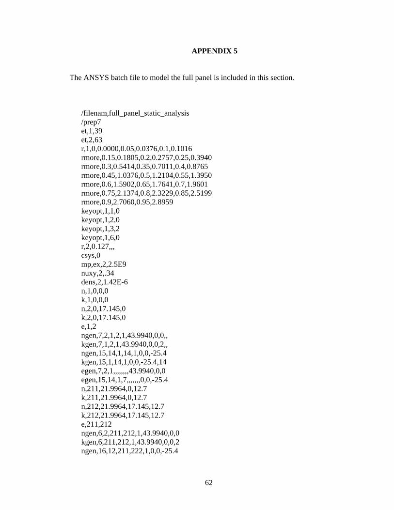
APPENDIX 5

The ANSYS batch file to model the full panel is included in this section.

/filenam,full_panel_static_analysis /prep7 et,1,39 et,2,63 r,1,0,0.0000,0.05,0.0376,0.1,0.1016 rmore,0.15,0.1805,0.2,0.2757,0.25,0.3940 rmore,0.3,0.5414,0.35,0.7011,0.4,0.8765 rmore,0.45,1.0376,0.5,1.2104,0.55,1.3950 rmore,0.6,1.5902,0.65,1.7641,0.7,1.9601 rmore,0.75,2.1374,0.8,2.3229,0.85,2.5199 rmore,0.9,2.7060,0.95,2.8959 keyopt,1,1,0 keyopt,1,2,0 keyopt,1,3,2 keyopt,1,6,0 r,2,0.127,,, csys,0 mp,ex,2,2.5E9 nuxy,2,.34 dens,2,1.42E-6 n,1,0,0,0 k,1,0,0,0 n,2,0,17.145,0 k,2,0,17.145,0 e,1,2 ngen,7,2,1,2,1,43.9940,0,0,, kgen,7,1,2,1,43.9940,0,0,2,, ngen,15,14,1,14,1,0,0,-25.4 kgen,15,1,14,1,0,0,-25.4,14 egen,7,2,1,,,,,,,,43.9940,0,0 egen,15,14,1,7,,,,,,,0,0,-25.4 n,211,21.9964,0,12.7 k,211,21.9964,0,12.7 n,212,21.9964,17.145,12.7 k,212,21.9964,17.145,12.7 e,211,212 ngen,6,2,211,212,1,43.9940,0,0 kgen,6,211,212,1,43.9940,0,0,2 ngen,16,12,211,222,1,0,0,-25.4

62

kgen,16,211,222,1,0,0,-25.4,12 egen,6,2,106,,,,,,,,43.9940,0,0 egen,16,12,106,111,,,,,,,0,0,-25.4 n,403,43.9928,0,25.4 k,403,43.9928,0,25.4 n,404,43.9928,17.145,25.4 k,404,43.9928,17.145,25.4 e,403,404 ngen,5,2,403,404,1,43.9940,0,0 kgen,5,403,404,1,43.9940,0,0,2 egen,5,2,202,,,,,,,,43.9940,0,0 n,413,43.9928,0,-381 k,413,43.9928,0,-381 n,414,43.9928,17.145,-381 k,414,43.9928,17.145,-381 e,413,414 ngen,5,2,413,414,1,43.9940,0,0 kgen,5,413,414,1,43.9940,0,0,2 egen,5,2,207,,,,,,,,43.9940,0,0 n,423,-21.997,0,-38.0999 k,423,-21.997,0,-38.0999 n,424,-21.997,17.145,-38.0999 k,424,-21.997,17.145,-38.0999 e,423,424 ngen,12,2,423,424,1,0,0,-25.4 kgen,12,423,424,1,0,0,-25.4,2 egen,12,2,212,,,,,,,,0,0,-25.4 ngen,2,24,423,446,1,307.95,0,0 kgen,2,423,446,1,307.95,0,0,24 egen,2,24,212,223,,,,,,,307.95,0,0 n,471,-43.9940,0,-76.2 k,471,-43.9940,0,-76.2 n,472,-43.9940,17.145,-76.2 k,472,-43.9940,17.145,-76.2 e,471,472 ngen,9,2,471,472,1,0,0,-25.4 kgen,9,471,472,1,0,0,-25.4,2 egen,9,2,236,,,,,,,,0,0,-25.4 ngen,2,18,471,488,1,351.952,0,0 kgen,2,471,488,1,351.952,0,0,18 egen,2,18,236,244,,,,,,,351.952,0,0 n,507,-65.991,0,-114.3 k,507,-65.991,0,-114.3 n,508,-65.991,17.145,-114.3 k,508,-65.991,17.145,-114.3 e,507,508

63

ngen,6,2,507,508,1,0,0,-25.4 kgen,6,507,508,1,0,0,-25.4,2 egen,6,2,254,,,,,,,,0,0,-25.4 ngen,2,12,507,518,1,395.946,0,0 kgen,2,507,518,1,395.946,0,0,12 egen,2,12,254,259,,,,,,,395.946,0,0 n,531,-87.988,0,-152.4 k,531,-87.988,0,-152.4 n,532,-87.988,17.145,-152.4 k,532,-87.988,17.145,-152.4 e,531,532 ngen,3,2,531,532,1,0,0,-25.4 kgen,3,531,532,1,0,0,-25.4,2 egen,3,2,266,,,,,,,,0,0,-25.4 ngen,2,6,531,536,1,439.94,0,0 kgen,2,531,536,1,439.94,0,0,6 egen,2,6,266,268,,,,,,,439.94,0,0 n,543,-117.988,0,-177.8 k,543,-117.988,0,-177.8 n,544,-117.988,17.145,-177.8 k,544,-117.988,17.145,-177.8 n,545,381.952,0,-177.8 k,545,381.952,0,-177.8 n,546,381.952,17.145,-177.8 k,546,381.952,17.145,-177.8 n,547,256.9964,0,-394.28 k,547,256.9964,0,-394.28 n,548,256.9964,17.145,-394.28 k,548,256.9964,17.145,-394.28 n,549,6.9964,0,37.98 k,549,6.9964,0,37.98 n,550,6.9964,17.145,37.98 k,550,6.9964,17.145,37.98 n,551,256.9964,0,37.98 k,551,256.9964,0,37.98 n,552,256.9964,17.145,37.98 k,552,256.9964,17.145,37.98 n,553,6.9964,0,-394.28 k,553,6.9964,0,-394.28 n,554,6.9964,17.145,-394.28 k,554,6.9964,17.145,-394.28 edele,202,212,1 edele,7,, edele,244,245,1 edele,268,269,1 edele,259,260,1

64

edele,223,224,1 edele,235,236,1 edele,253,254,1 edele,265,266,1 edele,1,, edele,99,, edele,271,, edele,105,, a,221,539,401,391,533,211 a,222,540,402,392,534,212 lsel,all lesize,all,,,30,,,,, type,2 real,2 mat,2 mshape,1,2-D mshkey,0 amesh,all nummrg,node,8e-3 allsel

65

APPENDIX 6

1. Force-displacement analysis results for full panel (Fig. 4.8).

Force (N)

Displacement (mm)

0.0000 0.0000 0.0981 0.0009 0.1962 0.0018 0.2943 0.0027 0.3924 0.0036 0.4905 0.0045 0.5886 0.0053 0.6867 0.0062 0.7848 0.0071 0.8829 0.0080 0.9810 0.0089

66

APPENDIX 7

1. FRF measured at point 1:

2. FRF measured at point 2:

0

2

4

6

8

10

12

0 10 20 30 40 50 60 70 80 90 100

Frequency (Hz)

Ampl

itude

(G^2

/Hz)

67

3. FRF measured at point 3:

4. FRF measured at point 4:

68

5. FRF measured at point 5:

6. FRF measured at point 6

69

7. FRF measured at point 7:

8. FRF measured at point 9 (FRF for point 8 not available):

70

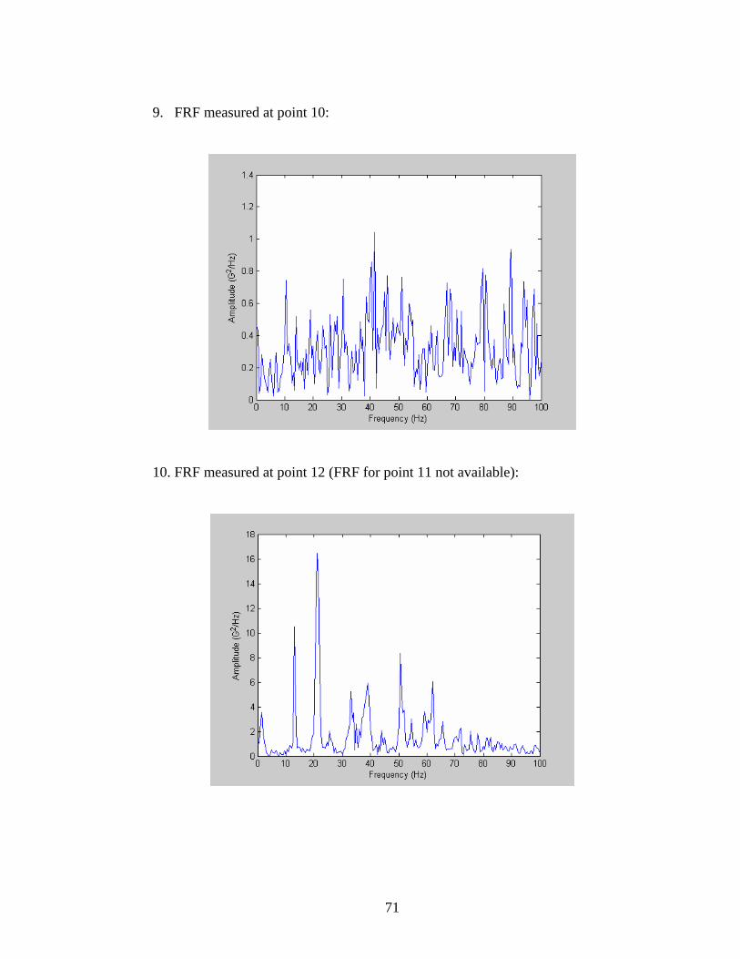
9. FRF measured at point 10:

10. FRF measured at point 12 (FRF for point 11 not available):

71

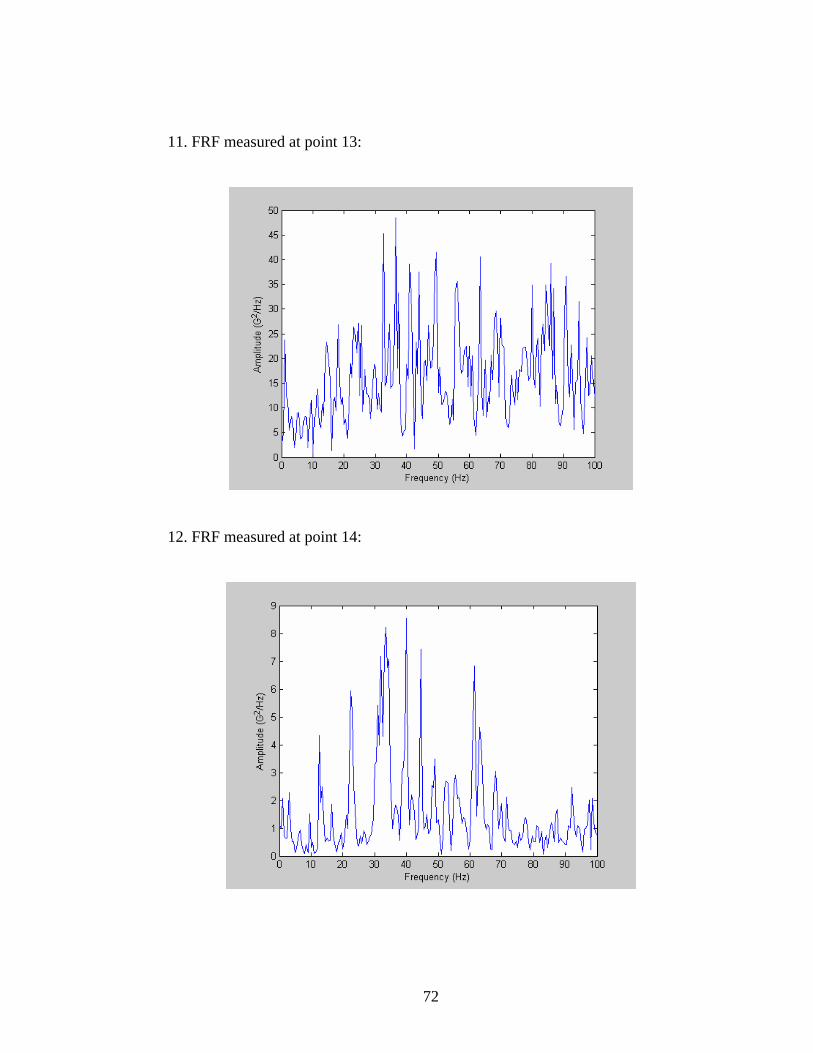
11. FRF measured at point 13:

12. FRF measured at point 14:

72

13. FRF measured at point 15:

Note: FRFs for points 16 – 24 not available.

73

APPENDIX 8

1. Mode shape 1 from modal analysis

2. Mode 2:

74

3. Mode 3:

4. Mode 4:

75

5. Mode 5:

6. Mode 6:

76

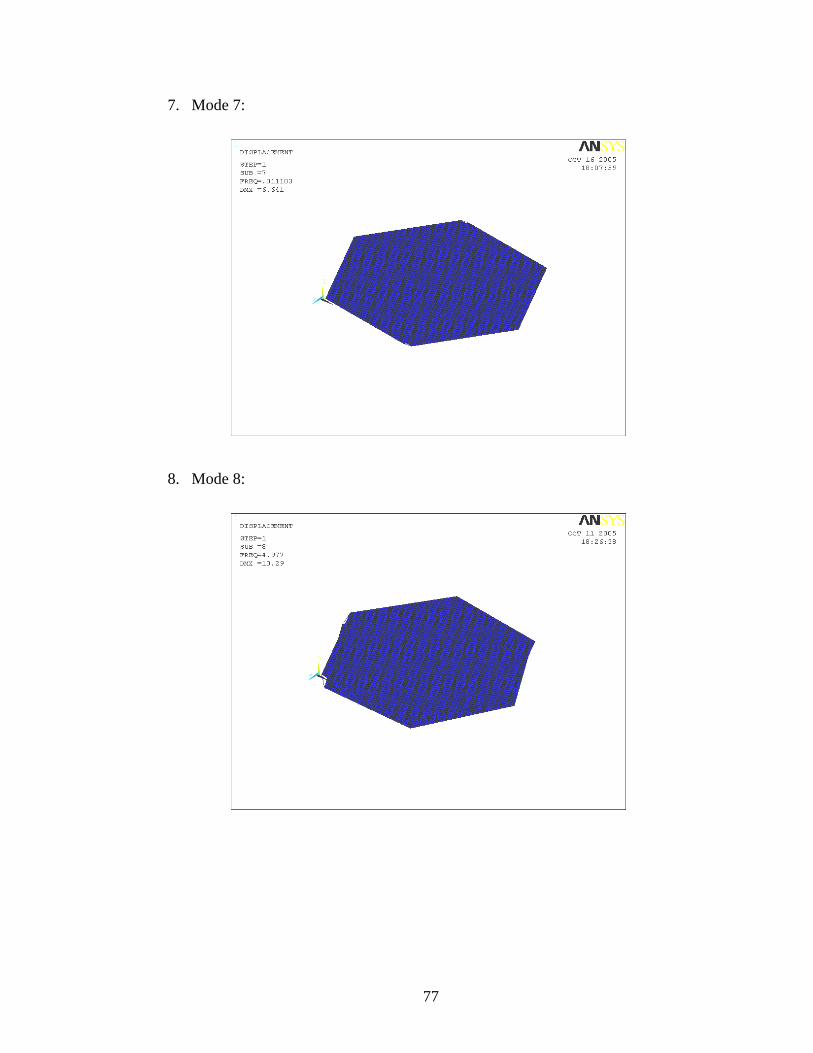
7. Mode 7:

8. Mode 8:

77

9. Mode 9:

10. Mode 10:

78

11. Mode 11:

12. Mode 12:

79

13. Mode 13:

14. Mode 14:

80

15. Mode 15:

16. Mode 16:

81

17. Mode 17:

18. Mode 18:

82

19. Mode 19:

20. Mode 20:

83

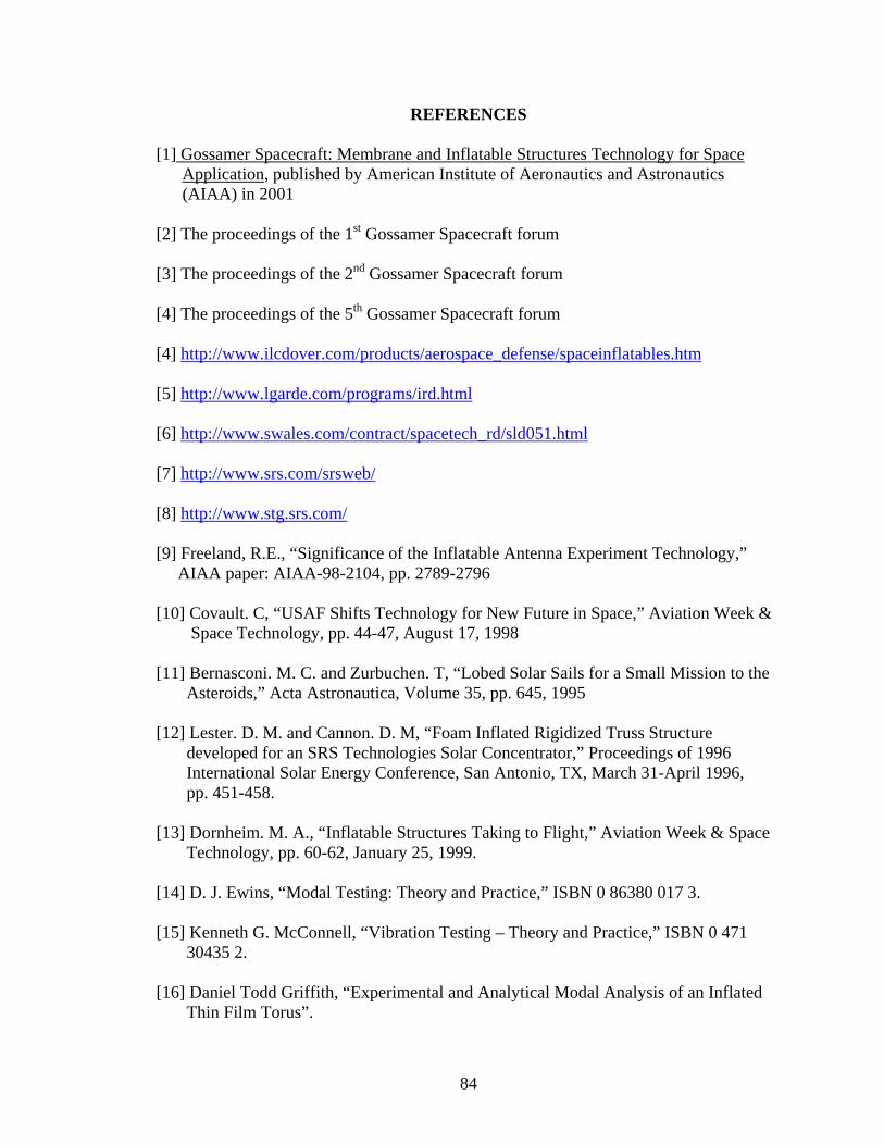
REFERENCES [1] Gossamer Spacecraft: Membrane and Inflatable Structures Technology for Space Application, published by American Institute of Aeronautics and Astronautics (AIAA) in 2001 [2] The proceedings of the 1st Gossamer Spacecraft forum [3] The proceedings of the 2nd Gossamer Spacecraft forum [4] The proceedings of the 5th Gossamer Spacecraft forum [4] http://www.ilcdover.com/products/aerospace_defense/spaceinflatables.htm [5] http://www.lgarde.com/programs/ird.html [6] http://www.swales.com/contract/spacetech_rd/sld051.html [7] http://www.srs.com/srsweb/ [8] http://www.stg.srs.com/ [9] Freeland, R.E., “Significance of the Inflatable Antenna Experiment Technology,” AIAA paper: AIAA-98-2104, pp. 2789-2796 [10] Covault. C, “USAF Shifts Technology for New Future in Space,” Aviation Week & Space Technology, pp. 44-47, August 17, 1998 [11] Bernasconi. M. C. and Zurbuchen. T, “Lobed Solar Sails for a Small Mission to the Asteroids,” Acta Astronautica, Volume 35, pp. 645, 1995 [12] Lester. D. M. and Cannon. D. M, “Foam Inflated Rigidized Truss Structure developed for an SRS Technologies Solar Concentrator,” Proceedings of 1996 International Solar Energy Conference, San Antonio, TX, March 31-April 1996, pp. 451-458. [13] Dornheim. M. A., “Inflatable Structures Taking to Flight,” Aviation Week & Space Technology, pp. 60-62, January 25, 1999. [14] D. J. Ewins, “Modal Testing: Theory and Practice,” ISBN 0 86380 017 3. [15] Kenneth G. McConnell, “Vibration Testing – Theory and Practice,” ISBN 0 471 30435 2. [16] Daniel Todd Griffith, “Experimental and Analytical Modal Analysis of an Inflated Thin Film Torus”.

84

[17] Richard S. Pappa, John O. Lassiter, and Brian P. Ross, ‘Structural Dynamics Experimental Activities in Ultra-Lightweight and Inflatable Space Structures”, NASA/TM-2001-210857 [18] Kara N. Slade, John O. Lassiter, “Dynamics of an Inflatable Structure in Vacuum and Ambient Conditions”, AIAA Journal, Vol. 39, No. 5, May 2001. [19] Eric Ruggiero and Daniel J. Inman, “Smart Materials in Inflatable Structure Applications”, AIAA Paper: AIAA 2002-1563. [20] Hendry A. Sodano and Daniel J. Inman, “Vibration Testing and Control of an

Inflatable Torus Using Multiple Sensors/Actuators”, AIAA Paper: AIAA 2003-1644.

[21] Suzanne W. Smith, “Larger Inflatable Self-Rigidizing Polymer Film Structures,” final report for contract project submitted to United Applied Technologies. [22] Jonathan T. Black, “Photogrammetry and Videogrammetry Methods Development for Solar Sails”. [23] Phani Krishnan Thota, “Pattern Evaluation for In-plane Displacement of Thin Films,” Masters Thesis work submitted at University of Kentucky, 2003. [24] Kin Fai Lore, “Efficient Computation of Dynamic Response of Large Inflatable Structures,” Masters Thesis, University of Kentucky, 2004. [25] Arthur L. Palisoc and Yuli Huang, ‘Design tool for inflatable space structures,” AIM-974 378. [26] L. Herbeck, M. Eiden, M. Leipold, C. Sickinger, W. Unckenbold, “Development and Testing of Deployable Ultra-Lightweight CFRP-Booms for a Solar Sail,” Proceedings of European Conference on Spacecraft Structures, November 2000. [27] Michael Lou and Houfer Fang, “A Combined Analytical and Experimental Study on Space Inflatable Booms,” Aerospace Conference Proceedings, 2000 IEEE. [28] Lawrie Virgin, “Nonlinear Analysis of Slender Booms for Solar Sails,” Duke University, Durham, NC.

85

VITA Prathik Navalpakkam Date of Birth: October 23, 1978 Place of Birth: Madurai, India Work experience: Fleetwood Enterprises Incorporated

Period: Aug 2004 – Present Title: Engineer – Recreational Vehicle Group

University of Kentucky, Mechanical Engineering Department

Period: July 2003 –Jul 2004 Title: Research Assistant

University of Kentucky, Mechanical Engineering Department

Period: Aug 2002 – June 2003 Title: Teaching Assistant

Caterpillar India Private Limited, India Period: Aug 1999 – June 2002 Title: Quality Engineer Education: Bachelor of Engineering in Mechanical Engineering, 1999 Bharadhidasan University, Tiruchirapalli, Tamil Nadu, India Professional Affiliations: July 2003 – July 2004 Society of Automotive Engineering (SAE) Student Member Sep 2000 – May 2002 Society of Automotive Engineering Board Member 86