modeling and simulation of high-speed milling centers dynamics · abstract high-speed machining is...

ORIGINAL ARTICLE

Modeling and simulation of high-speed millingcenters dynamics

El Bechir Msaddek & Zoubeir Bouaziz & Maher Baili &Gilles Dessein

Received: 9 June 2010 /Accepted: 3 August 2010 /Published online: 29 August 2010# The Author(s) 2010. This article is published with open access at Springerlink.com

Abstract High-speed machining is a milling operation inindustrial production of aeronautic parts, molds, and dies.The parts production is being reduced because of theslowing down of the machining resulting from the toolpath discontinuity machining strategy. In this article, wepropose a simulation tool of the machine dynamicbehavior, in complex parts machining. For doing this,analytic models have been developed expressing thecutting tool feed rate. Afterwards, a simulation method,based on numerical calculation tools, has been structured.In order to validate our approach, we have compared thesimulation results with the experimental ones for thesame examples.

Keywords Machining . Pocket . Modeling . Simulation .

HSM

NomenclatureVf(t) Instantaneous feed rateV!

Feed rate vectorVft Tangential feed rateVfprog Programmed feed rateVftcy Feed rate imposed by tcyVflsacc Feed rate for static look ahead imposed by the

accelerationVflsjerk Feed rate for static look ahead imposed by the

jerkVs Feed rate for static look aheadVst Feed rate for modified static look aheadVf(i) Feed rate of a block (i)Vmax Maximal feed rateVmaxi Maximal feed rate of axis (i)A(t),Af Instantaneous feed accelerationA!

Feed acceleration vectorAt Tangential accelerationAn Normal accelerationAmax Maximal accelerationAmaxi Maximal acceleration of axis (i)J(t) Instantaneous feed JerkJ!

Jerk vectorJt Tangential JerkJc Normal JerkJmax Maximal JerkJmaxi Maximal Jerk of axis (i)Jcurv Curvilinear tangential JerkJtcurv Tangential Jerk on curvaturerjct Rate of curvilinear jerk associated of tangential

jerktcy Time of interpolation cycleTIT(*) Interpolation tolerance of trajectoryδt Crossing time of discontinuity

E. B. Msaddek (*) : Z. BouazizUnit of Research of Mechanics of the Solids,Structures and Technological Development, ESSTT,Tunis, Tunisiae-mail: [email protected]

Z. Bouazize-mail: [email protected]

M. Baili :G. DesseinLaboratory Production Engineering,National School of Engineers of Tarbes,47 Avenue Azereix, BP 1629, 65016 Tarbes Cedex, France

M. Bailie-mail: [email protected]

G. Desseine-mail: [email protected]

Int J Adv Manuf Technol (2011) 53:877–888DOI 10.1007/s00170-010-2884-z

R,R(s) Curvature radiusRj Curvature radius of block (j)L,Ltraj Length of the tool pathLi Length of the tool path of a block (i)β Angle between two blocksβj Angle of a block (j)α Angle between a block and the machine axisαj Angle between a block (j) and the machine axisd Distancedacc Acceleration distanceddec Deceleration distance

1 Introduction

High-speed milling (HSM) has very interesting character-istics in the scope of the realization of high-qualitymechanical parts in automobile industry and aeronautics[1]. The complex parts machining in HSM allows to takeoff the maximum material in the minimum time [2]. Thecost of the part is then reduced [3], since the machiningtime represents an important part of the cost price.

The conception and the ordering of numerical drive toolmachines necessitate the development of certain mathemat-ical models [4]. The transformation models, between thework space and the dynamic models, defining the motionequations of the tool machine, allow the establishment ofthe relations between the couples or forces exerted by theactuators, and the positions, the speeds, and the accelerationof the axis articulations [5].

The geometrical shape influences the trajectories. Thelatter, characterized by speeds and accelerations, will betreated by the Numerical Controlled Unit (NCU) and willengage a certain imprecision (machine behavior) [6]. Thus,the dynamic modeling becomes a necessity for themachining optimization [7].

Recent studies have been interested in the HSM machinesbehavior modeling for pockets and complex shapes machin-ing. Monreal et al. [4] and Tapie et al. [7] have treated theinfluence of the tool trajectory upon the machining time inHSM. Guardiola et al. [8] and Souza et al. [9] have evaluatedthe speed rate oscillation while machining and its influenceupon the part obtaining time as well as upon its surfacequality. Moreover, Souza et al. [9] have considered theinfluence of the tolerance value provided by the CAMsoftware for the calculation of the desired tool trajectory.

Dugas [10] and Pateloup et al. [11, 12] have integratedthe dynamic modeling of HSM machines by justifying thevariation applied to the feed rate. Some parameters like thejerk, the acceleration, and the time of interpolation cyclehave been used in order to make the machine slowing downin linear and circular interpolation explicit. Thus, Mawussi

et al. [7] and Pateloup [13] have included the HSMmachine real behavior study in the pocket hollowing out.Thus, other interpolations like B-spline are tested with the840 D Siemens controller.

In most studies, the feed rate variation is not justified;this is one of the aims of this paper. Besides, there are noother studies which numerically examine and analyze thetool trajectory influence in CAM upon the HSM machinefeed rate for the pockets hollowing out.

In this article, we present a feed rate calculation dynamicmodel according to the tool trajectory. This modelingincludes the jerk, the acceleration, and the interpolationcycle time. Then, we simulate the feed rate for a pockethollowing out and for a complex part machining with the840 D Siemens controller.

In the first part, the detailed dynamic models develop-ment of both the axis and controller permits to betterexpress the real behavior of the HSM tool machine. In thesecond part, the exploitation of the modeling for the realmachining feed rate simulation is realized in the case of twoparts of different shapes.

2 The tool-machine NC dynamic modeling in HSM

2.1 Modeling step

The dynamic modeling of the numerical drive HSM toolmachine necessitates essentially the modeling of both theNCU controller and the motions axis.

The NCU behavior modeling is carried out through threesteps. First of all, the integration of the connecting arcs ismodeled. This is the phase of the tool trajectory preparation.Afterwards, the “Static Look Ahead” is also modeled. Withthis criterion, The NCU imposes the adequate speed in costumetime, taking into account the axis capacities (axis modeling).Then, the “Dynamic Look Ahead” is modeled. It is the NCUcapacity to anticipate in speed and acceleration during themachining to avoid the sudden acceleration (path overrun).

The modeling step is represented in the following diagram:(Figure 1)

HSM machineModeling

NCU Modeling AXIS Modeling

Preparation dy arc of circle

Static Look Ahead

Dynamic Look Ahead

Fig. 1 A HSM machine dynamic modeling step

878 Int J Adv Manuf Technol (2011) 53:877–888

2.2 NCU behavior modeling

2.2.1 Tool path modeling by arc of circle

In CAM, the tool path C0 (Fig. 2a) presents sharp angleswhile changing direction. In HSM machining, this suddenchange necessitates the violent deceleration and thestopping of the machine for the crossing of tangentialdiscontinuity. The NCU integrates connecting arcs in orderto solve this problem. We obtain, then, the modifiedtrajectory C1 with continuity in tangency (Fig. 2b).

Figure 3 presents the construction of connection radiusbetween the three blocks (i−1), (i), and (i+1) of respectivelengths Li+1, Li, and Li−1. The radius expression Rj of theconnection between two blocks takes into account the angleof passage between the block (i−1) and the block (i) βj, ofthe trajectory interpolation tolerance TIT* and of the mini.Length between Li and Li−1 [1].

Rj ¼ MINTIT»

tanbj2

� � ; L

2 tanbj2

� � � TIT»

0@

1AWith L¼ MIN Li ; Li�1ð Þ

ð1ÞThe passage of the tangential discontinuity maximal feed

rate depends on the integrated arc radius. The arc radius Rleads to a more important speed limitation for the weakvalues of the β angle and also to a less strong speed limitfor the greater values of the same angle.

Considering that the arc of circle of a radius R is crossedwith a maximal tangential jerk Jmax (derived from theacceleration), the maximal feed rate passage of the blocktransition is proportional to Jmax [7].

This speed depends on the arc radius and so it dependson the Eq. 1 of the angle between the two segments β andthe tolerance TIT*.

Consequently, the maxi jerk Jmax depends on the toolpath. In this case, we can have two types of configuration:

& Case of curvature discontinuity between a segment andan arc, C1 discontinuity (Fig. 4):

In this case, the jerk is according to the axis directions(α: angle between the axis and the reference machineXm�!

; Ym�!� �

). The covered trajectory is ABCD whichrepresents three blocks and a relative reference t!; n!

� �.

The maximal jerk at the point B is given by [7]:

JmaxðBÞ ¼ minJmaxX

cos að Þj j ;JmaxY

sin að Þj j� �

ð2Þ

& Case of curvature discontinuity between two arcs ofcircle of radius R1 and R2 connected in tangency, C2

discontinuity, (Fig. 5):

The crossing speed determination method of thisdiscontinuity Vf, is as follows [12]:

The positionRðsÞ ¼ Rr1 a t� dt et RðsÞ ¼ Rr2 a tþ d t

With δt: time of the discontinuity crossing.The tangential acceleration is nil on the curvature

discontinuity. Well, the normal acceleration varies and canbe written on the basis of Frenet ðn;�! t!Þ as follows:

A!

t þ dt2

� �� A!

t � dt2

� �¼ Rr1 � Rr2ð Þ:V 2

f

Rr1Rr2

!N!

f

¼ jcmax:dtð ÞN!f ) Vf ¼ffiffiffiffiffiffiffiffiffiffiffiffiffiffiffiffiffiffiffiffiffiffiffiffiffiffiffiffiffiffiffijcmax:dt:Rr1:Rr2

Rr1 � Rr2j j

sð3Þ

(b)(a)

C0 C1 Radius of connecting

Fig. 2 Tangential discontinuityand connecting with arcs ofcircle

Rj

βj

Li-1

Li

Li+1

Block (i-1) Block (i) Block (i+1)

TIT

α i-1 αi

Rj+1

βj+1

αi+1

TIT*

Fig. 3 Trajectory modeling by arc of circleFig. 4 Curvature discontinuity between two segments and an arc inthe plan (X, Y) [7]

Int J Adv Manuf Technol (2011) 53:877–888 879

2.2.2 Static look ahead

The HSM machine has at its disposal the interpolationaxis X, Y, and Z which are different at the level oftheir dynamic capacities. Each axis [i] has a maximalspeed Vmaxi, a maximal acceleration Amaxi, and amaximum jerk Jmaxi. These capacities depend on theengines and on the loads characteristics. In shapemachining, we are then limited by the less dynamic (lessrapid) axis i:

Vmax¼min Vmaxið Þ; Amax¼min Amaxið Þ; and Jmax¼min Jmaxið Þð4Þ

There are different types of feed rate limitations. If thetrajectory is of class C0, the controller algorithm carries outthe following calculations for each block:

Vftcy ¼ min Vfprog ; L=tcy� ð5Þ

This calculation puts into evidence the programmedspeed Vfprog, the block length L, and the interpolation cycletime tcy. The block machining time must not be inferior tothe tcy. So, the speed will be minimized if L is very small(t < tcy).

If the trajectory is of class C1, the limitations ofspeed in circular interpolation, in the plan XY, arecalculated for each angular position on the arc of circleof a radius R. In this way, the following calculationsdetermine the most restrictive axis in speed, in acceler-ation, and in jerk:

Vft ¼ min VmaxXcos aið Þj j ;

VmaxYsin aið Þj j

� �

An ¼ min AmaxXcos aið Þj j ;

AmaxYsin aið Þj j

� �pour ai 2�

Jt ¼ min JmaxXcos aið Þj j ;

JmaxYsin aið Þj j

� �� 0:b� ð6Þ

Vftcy ¼ R� btcy

ð7Þ

The acceleration is composed of tangential accelerationat and of a normal one an in the basis of Frenet ðn;�! t!Þ [11].

A!¼ dVf

�!dt ¼ dVf ðtÞ

dt :T!þ Vf

2ðtÞR :N

!At ¼ dVf ðtÞ

dt andAn ¼ Vf2

R

ð8Þ

For a linear block At ¼ dVf ðtÞdt

and An ¼ 0 ð9Þ

If the feed rate is constant, the corresponding accelera-tion is only normal An [14]. Then, so as the machine canfollow a curve of a curvature radius R, at an imposed feedrate Vf, we must necessarily have:

An � V 2f=R ð10Þ

When this relation cannot be satisfied, the controllerremakes the feed rate calculation in static look ahead linkedto the acceleration Vflsacc, we have, then:

Vflsacc ¼ffiffiffiffiffiffiffiffiffiffiffiffiffiffiR� An

pð11Þ

On the other hand, a small curvature radius induces acurvature jump and consequently an important couple ofdeceleration/acceleration accompanied by an infinite variationof jerk. In these different cases, a jerk limitation is used [11].

Fig. 5 Curvature discontinuitybetween two arcs of circle [12]

B C

D A

Ri

Ri-1

Block i

Block i-1

Block i+1Trajectory

Speed profile

Variable acceleration Variable deceleration

CurvilinearPosition

Vf

Vfi

Vfendi-1

Vfendi

0 S0i S1i S2i S3i S1i

A B C D . . . .

Fig. 6 Correspondence between the trajectory and the speed profile


The jerk is the acceleration derivative. Each accelerationcomponent is controlled by a tangential jerk Jt and a centripetaljerk Jc. In the stationary state of the speed dA

dt ¼ 0, Eq. 12 showsthat the jerk is tangential Jt. Hence, the maximal jerk Jmaxi of theaxis i limits the value of the tangential jerk Jt.

J!¼ d A

!dt

! J!¼ dA

dtN!þ A

dN!dt

¼ J!

t ð12Þ

According to (8) and (9):

J!¼ d A

!dt

¼ dA

dtN!þ A

dN!dt

¼ V 2f

R:Vf

R:T!¼ V 3

f

R2:T!¼ Jt

! ð13Þ

For a feed rate Vf imposed, we must necessarily have:

Jmax ¼ Jt � V 3f =R

2 ð14ÞWhen this relation cannot be satisfied, the controller

recalculates the feed rate in static look ahead linked to thejerk Vflsjerk, then we have:

Vflstjerk ¼ 3ffiffiffiffiffiffiffiffiffiffiffiffiffiffiJt � R2

pð15Þ

The feed rate Vs representing the minimum differentlimitation types is called static look ahead.

Vs ¼ min Vfprog;Vftcy;Vft;Vflsacc;Vflstjerk

� ð16ÞTapis et al. [14] add the effects of the tangential jerk in

curvature Jtcurv and prove its limitation effect by theexperimental. The tangential jerk in curvature is the productof the curvilinear tangential jerk Jcurv and of the rate of thecurvilinear jerk associated to the tangential jerk rjct.

Jtcurv ¼ Jcurv � rjct ) Vjtcurv ¼ 3ffiffiffiffiffiffiffiffiffiffiffiffiffiffiffiffiffiffiffiffiJtcurv � R2

pð17Þ

Afterwards, the feed rate Vst representing the minimumof the different limitation types is called: modified staticlook ahead.

Vst ¼ min Vfprog;Vftcy;Vft;Vflsacc;Vflstjerk;Vjtcurv

� ð18Þ

The static look ahead well describes the machine dynamicbehavior, but this feed rate calculation is done in costume timefor the running block unaware of the following block (oldmachines). These problems are resolved by the integration ofthe dynamic look ahead (modern machines), in such a waythat the NCU becomes able to anticipate the trajectory for thenext 200 blocks. In fact, with the anticipation, we can avoidthe overtaking caused by violent decelerations.

2.2.3 Dynamic look ahead

The term “dynamic” means that we need to calculate thespeed profile with its two deceleration/acceleration phaseson the running block. The dynamic look ahead permits thento anticipate in speed and in acceleration, thanks to theknowledge of the next blocks. In the case of any speedprofile, the modeling is diagrammed in Fig. 6.

➢ Calculation model of the acceleration and deceler-ation distance

The NC tool machine axis does not allow the sameacceleration distance, according to the speed thresholds

A (0,70)

B (0,50) C

D

E (200,0)

F (150,-50)

Y

X

Tool path direction

G

R 20

R 50

Fig. 8 Tested trajectory [15]

Geometry of the part for machining

CAD

Manufacture the partCAM MASTERCAM

Generate a NC file

Integrate a dynamicmodels

Simulate the feed rateMATLAB

Cut

Conditions

Fig. 7 Modelizing and simulation global step


where it is located. For example, the distance covered bythe machine is shorter if it accelerates from 13 to 15 m/min,comparatively to an acceleration of 11 to 13 m/min. Toreach the programmed speed, the machine covers theacceleration distance dacc during the time tcy. Likewise forthe deceleration, in order to cancel the feed rate or todiminish it, the machine covers the deceleration distanceddec during the time tcy according to the following Eq. 20:

Vfprog ¼ d

tcyð19Þ

Pateloup [13] shows that in HSM conditions, if thedistance to cover between two successive information isinferior to 3 mm, then the feed rate falls until 50%. For blocki, the model of the distances dacc and ddec is the following:

daccðiÞ ¼ Vf ðiÞ � Vf i� 1ð Þð Þ � tcy ð20Þ

ddecðiÞ ¼ Vf ðiÞ � Vf ðiþ 1Þð Þ � tcy ð21ÞA HSM machine is made up of several components

(axis, controller…) having their own limits and whichinteract between themselves. This makes the machinemodeling dependent on several parameters.

The structured dynamic modeling will be programmedwith Matlab© in order to develop a feed rate simulator.This is the objective of the following part.

3 HSM machining simulation

In a first stage, we are determined to simulate the millingphenomena put at work. In a second period, tests on machinesare realized so as to correlate the simulations with the reality.

In order to study the influence of the HSM machinedynamic behavior in milling, we start by developing the CAMmodel and the generation of a NC file. Then, we simulate the

tool trajectories with Matlab© by using the NC file alreadydeveloped by the CAM model. Afterwards, we represent thecorresponding feed rate profiles in static look ahead and indynamic look ahead. Finally, we compare the simulated feedrate profiles with those of the experimental statements.

3.1 Simulation step

The step is represented in the following diagram (Fig. 7):This step includes five main stages:

1. Conceive the part in CAD with SolidWorks©.2. Develop the part CAM model with Mastercam©.3. Generate the NC file useful for the simulation tool.4. Integrate the dynamic models:

4.1 Trajectory preparation by using the trajectoryInterpolation Tolerance TIT.

4.2 Calculation of the static look ahead type on thetrajectory (Ac/deceleration/jerk/feed rate. maxi. /axis + interpolation cycle time).

4.3 Calculation of the dynamic look ahead type on thetrajectory (Ac/deceleration/jerk.. maxi. /axis +look ahead).

4.4 Storage of speed constraints for each block (staticlook ahead).

Fig. 10 Pocket obtained by Mastercam©

raw

raw

raw

raw

pocket

Pocket contourTested trajectory

Fig. 9 Machining strategy inconvergent parallel Spirals(Mastercam©)


4.5 Storage of the instruction of the imposed antici-pated speed at each axis according to thecurvilinear abscissa (dynamic look ahead).

5. Make the speed (feed rate) profile withMatlab© software.

3.2 Machining simulation of a complex shape test pocket

3.2.1 Pocket definition

A trajectory proposed by Cherif (Fig. 8) [15] has been testedon a HSM machining center (IUT of Nantes / HERMLEC800U 5 axis—HENDENHAIN TNC430—Acceleration5 m/s²), for two programmed feed rates from 15 to 35 m/min. The tests have permitted to record the real feed rateduring the time. A confrontation between the simulation

results and the experimental results will be realized in orderto validate the developed simulation model.

3.2.2 Hollowing out, strategy, and pocket characteristics

➢ Hollowing out and strategy

The rough piece is prismatic of dimensions (300×200×20), the axial pass depth is of 10 mm. The tool used is adouble cut milling tool of a diameter Ø 20. The otherparameters are taken by default.

Figure 9 presents the rough piece, the pocket, and thehollowing out strategy in convergent parallel spirals.

The final pocket obtained by Mastercam© is presentedin 3D in Fig. 10.

➢ Pocket characteristics

-50 0 50 100 150 200

-60

-40

-20

0

20

40

60

80

Pocket length (mm)

Po

cket

wid

th (

mm

)

Prepared trajectory

A

BC

D

E

FG

Fig. 12 Modified tool trajectory

-50 0 50 100 150 200-60

-40

-20

0

20

40

60

Pocket length (mm)

Po

cket

wid

th (

mm

)

Tool path (parallel spiral)

A

B C

D

E

FG

Fig. 11 Tool path simulatedwith Matlab©


The geometry of this pocket allows us to test theinterpolation G1, G2 and to solicit one or several axissimultaneously:

❖ Test the monoaxial linear interpolation G1 (portionsAB, BC, DE, and FG of the trajectory tested on thefirst machining pass (Fig. 9)).❖ Test the bi-axial linear interpolation G1 (EF).❖ Test the circular interpolation G2 (the long radiusGB and the small radius CD...)❖ Test the tangencial discontinuities (of speed) of axischange (point B...).❖ Test the curvature discontinuities (of acceleration inC, D and G points...)

3.2.3 Real feed rate simulation

➢ Trajectory definition

We start with the tool path simulation representing thepocket hollowing out operation. It is realized withMatlab© after the reading of the Mastercam© NC file(Fig. 11).

The total length of the pocket machining trajectory Ltrajis calculated by the numerical simulator. Ltraj=2,300.7 mm.

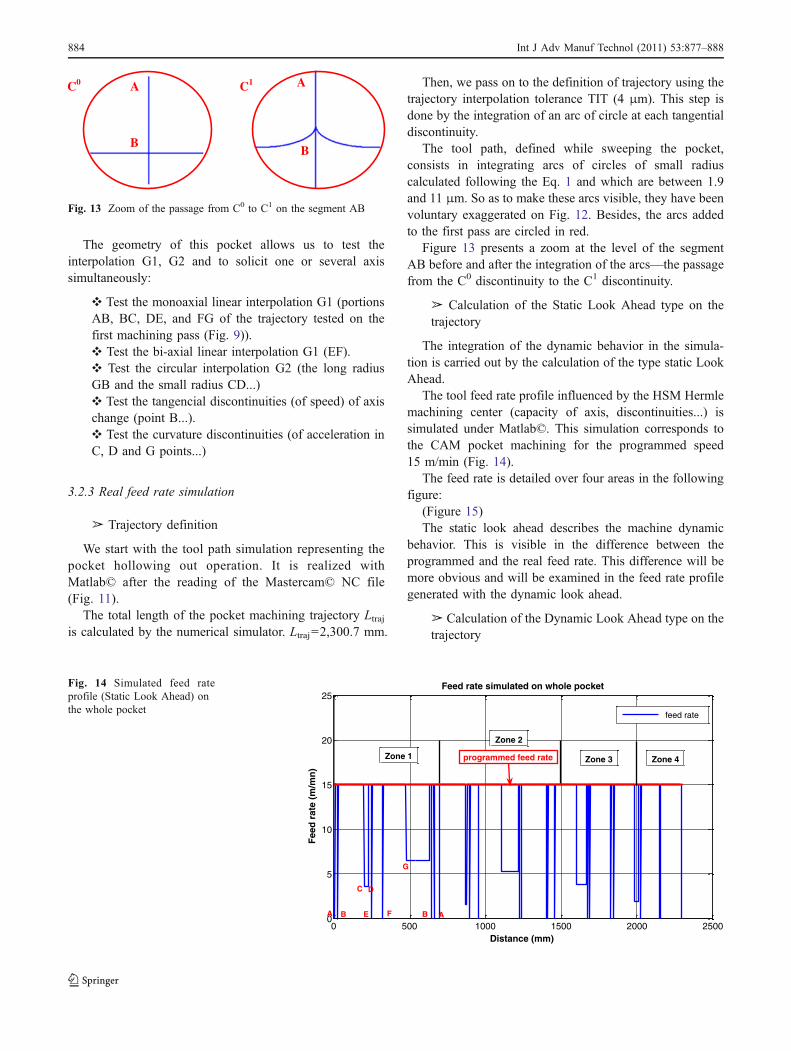
Then, we pass on to the definition of trajectory using thetrajectory interpolation tolerance TIT (4 μm). This step isdone by the integration of an arc of circle at each tangentialdiscontinuity.

The tool path, defined while sweeping the pocket,consists in integrating arcs of circles of small radiuscalculated following the Eq. 1 and which are between 1.9and 11 μm. So as to make these arcs visible, they have beenvoluntary exaggerated on Fig. 12. Besides, the arcs addedto the first pass are circled in red.

Figure 13 presents a zoom at the level of the segmentAB before and after the integration of the arcs—the passagefrom the C0 discontinuity to the C1 discontinuity.

➢ Calculation of the Static Look Ahead type on thetrajectory

The integration of the dynamic behavior in the simula-tion is carried out by the calculation of the type static LookAhead.

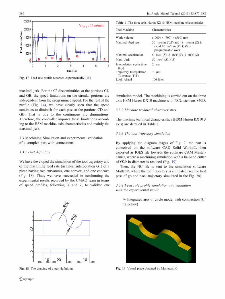
The tool feed rate profile influenced by the HSM Hermlemachining center (capacity of axis, discontinuities...) issimulated under Matlab©. This simulation corresponds tothe CAM pocket machining for the programmed speed15 m/min (Fig. 14).

The feed rate is detailed over four areas in the followingfigure:

(Figure 15)The static look ahead describes the machine dynamic

behavior. This is visible in the difference between theprogrammed and the real feed rate. This difference will bemore obvious and will be examined in the feed rate profilegenerated with the dynamic look ahead.

➢ Calculation of the Dynamic Look Ahead type on thetrajectory

0 500 1000 1500 2000 25000

5

10

15

20

25

Distance (mm)

Fee

d r

ate

(m/m

n)

Feed rate simulated on whole pocket

programmed feed rate

feed rate

Zone 1

Zone 2

Zone 3 Zone 4

A B

C D

E F

G

B A

Fig. 14 Simulated feed rateprofile (Static Look Ahead) onthe whole pocket

Fig. 13 Zoom of the passage from C0 to C1 on the segment AB


The dynamic look ahead allows to anticipate in speedand in acceleration. Thanks to the knowledge of thefollowing blocks, the NCU calculates the speed profilewith its acceleration and deceleration phases on eachblock, taking into account the speed profile in the nextblock. A calculation model of the acceleration anddeceleration distance of each block, by taking intoaccount the preceding and the following speeds, isintegrated in our simulator.

In fact, with the anticipation, we can avoid theovertaking caused by the violent decelerations. The feedrate profile, simulated with the dynamic look ahead and theparameters of HSM machining center Hermle C800U 5 axis(jerk 0.5 m/s3), on the trajectory ABCDEFG (Fig. 11), isshown in Fig. 16. Then a comparaison with the experimen-tal statement (Fig. 17) for the same trajectory tested on theHSM MC Hermle, is realized with the same programmedfeed rate 15 m/min.

We notice the influence of the anticipation on the speedprofile in comparison to that of the static look ahead. Thedecelerations are known in advance and are carried out onthe current blocks. That really describes the recent HSMdynamic machines behavior.

The speed profile simulated (Fig. 16) on the testtrajectory (Fig. 8) is very near (2% of error) to the profileof the experimental statement (Fig. 17).

On the C0 discontinuities at the points B, E, and F, thefeed rate is very near to 0. These speed limitations are dueto the passage of the tool by the small connection radius.More precisely, the speed is limited by the machine

0 100 200 300 400 500 6000

5

10

15

20

25

distance (mm)

Fee

d r

ate

(m/m

in)

feed rate

A B

C D

E F

G

B A

programmed feed rate

Vf prog : 15 m/min

Fig. 16 Real feed rate profile simulated with the dynamic look aheadon the trajectory ABCDEFG

100 200 300 400 500 600 700 800

10

15

20

25

Distance (mm)

Fee

d r

ate

(m/m

n)

10

15

20

25

Fee

d r

ate

(m/m

n)

10

15

20

25

Fee

d r

ate

(m/m

n)

10

15

20

25

Fee

d r

ate

(m/m

n)

Feed rate simulated on whole pocket Feed rate simulated on whole pocket

Feed rate simulated on whole pocket Feed rate simulated on whole pocket

feed rate

Zone 1

800 900 1000 1100 1200 1300 1400 1500Distance (mm)

Distance (mm) Distance (mm)

feed rate

Zone 2

1500 1550 1600 1650 1700 1750 1800 1850 1900 1950 2000

feed rate

Zone 3

2000 2050 2100 2150 2200 2250 2300 2350

feed rate

Zone 4

5

00

5

0

5

0

5

0

A B

C D

E F

G

B A

Fig. 15 Simulated feed rate profile (static look ahead) detailed over four areas


maximal jerk. For the C1 discontinuities at the portions CDand GB, the speed limitations on the circular portions areindependent from the programmed speed. For the rest of theprofile (Fig. 14), we have clearly seen that the speedcontinues to diminish for each pass at the portions CD andGB. That is due to the continuous arc diminutions.Therefore, the controller imposes these limitations accord-ing to the HSM machine axis characteristics and mainly themaximal jerk.

3.3 Machining Simulation and experimental validationof a complex part with connections

3.3.1 Part definition

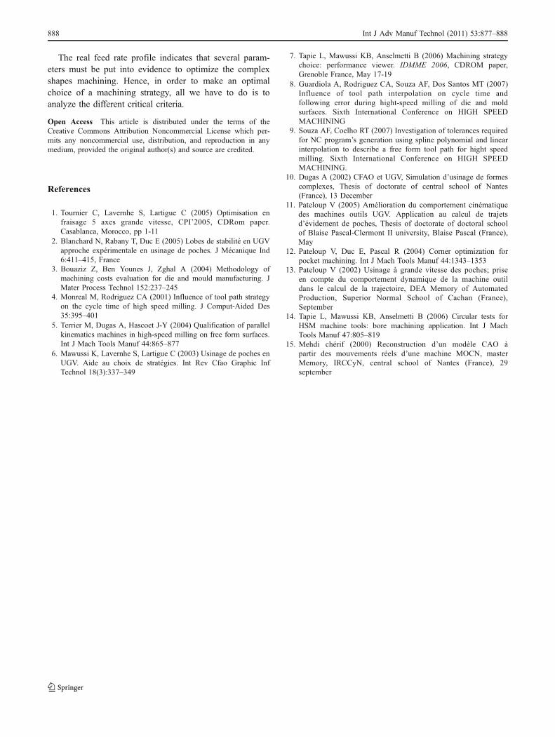
We have developed the simulation of the tool trajectory andof the machining feed rate (in linear interpolation G1) of apiece having two curvatures, one convex, and one concave(Fig. 18). Thus, we have succeeded in confronting theexperimental results recorded by the CMAO team in termsof speed profiles, following X and Z, to validate our

simulation model. The machining is carried out on the threeaxis HSM Huron KX10 machine with NCU siemens 840D.

3.3.2 Machine technical characteristics

The machine technical characteristics (HSM Huron KX10 3axis) are detailed in Table 1.

3.3.3 The tool trajectory simulation

By applying the diagram stages of Fig. 7, the part isconceived on the software CAD Solid Works©, thenexported as IGES file towards the software CAM Master-cam©, where a machining simulation with a ball-end cutterof Ø20 in diameter is realized (Fig. 19).

Then, the NC file is sent to the simulation softwareMatlab©, where the tool trajectory is simulated (see the firstpass of go and back trajectory simulated in the Fig. 20).

3.3.4 Feed rate profile simulation and validationwith the experimental result

➢ Integrated arcs of circle model with compaction (C1

trajectory)

Table 1 The three-axis Huron KX10 HSM machine characteristics

Tool-Machine Characteristics

Work volume (1000) × (700) × (550) mm

Maximal feed rate 30 m/min (X,Y) and 18 m/min (Z) inrapid 10 m/min (X, Y, Z) inprogrammable work

Maximal acceleration 5 m/s² (X), 5 m/s² (Y), 3 m/s² (Z)

Maxi. Jerk 50 m/s3 (X, Y, Z)

Interpolation cycle time(tcy)

2 ms

Trajectory InterpolationTolerance (TIT)

7 μm

Look Ahead 100 lines

Fig. 18 The drawing of a part definition

A B C D E FG

B A

Vf prog : 15 m/min

Time (s)

Fee

d ra

te (

m/m

n)

Fig. 17 Feed rate profile recorded experimentally [15]

Fig. 19 Virtual piece obtained by Mastercam©


The feed rate profile generation in linear interpolation onMatlab© passes then by the dynamic modeling of the NCUof the HSM machine. One of the crossing models oftangential discontinuities is the integration of arcs betweentwo linear blocks. Since the whole part machiningtrajectory is in linear interpolation, we adopt this model toestimate the NCU behavior, badly mastered during thepassage of the tangential discontinuities. Besides, the NCUachieves the blocks compaction of small blocks into 5 mmsegments. Afterwards, we are going to simulate the feedrate profile and compare it with that of the experimentalstatement.

➢ Feed rate profile

Figure 21 presents the simulated and the measured feedrate profiles .The experimental statement speed profile forthe Huron KX10 is measured for a set speed of 9.6 m/min.

➢ Comparison of the simulation result and theexperimental statement

We have simulated a speed profile by the arcs of circleintegration model, with compaction. This profile is verynear (5% of error) the experimental statement profile. But,there are some differences caused by a slight trajectorydiscretization. Hence, we notice that the compaction hasconserved a more important value of the feed rate, for itconsists in compacting the blocks of small segments whichprovoke the slowing down of the machine, imposed by theinterpolation cycle time tcy. If we have less compaction, wewill get more slowing down and consequently a greatermachining time.

4 Conclusion

In this article, we have been interested in machiningsimulation of a pocket and of a complex profile. Theobjective is to introduce the dynamic modeling of the HSMmachine in the simulation of a given trajectory.

In a first step, we have detailed the HSM machiningcenter dynamic modeling. Then, we have explained thepassage of the CAM model towards numerical simulationsoftware, passing through the modeling. In a second step,we have simulated the real feed rate of a pocket hollowingout.

In the second part, we have been interested in the feedrate simulation of a complex part machining, in order toshow the anticipation influence with compaction. We havediscovered that the speed is variable according to the shapeto be machined and the anticipation keeps a more importantspeed evolution.

Afterwards, we come to the conclusion that thesimulation tool which permits to give values very near thereality (≤5% of errors) for the pocket hollowing out and forthe complex part machining.

Fig. 21 Feed rate profilesimulated and measured onmachine

-10 0 10 20 30 40 50 60 70

5

10

15

20

25

30

35

40

Length of part (mm)

hei

gh

t o

f p

art

(mm

)tool path in machining (zig-zag one pass) in linear interpolation

Fig. 20 A go-and-back simulated trajectory


The real feed rate profile indicates that several param-eters must be put into evidence to optimize the complexshapes machining. Hence, in order to make an optimalchoice of a machining strategy, all we have to do is toanalyze the different critical criteria.

Open Access This article is distributed under the terms of theCreative Commons Attribution Noncommercial License which per-mits any noncommercial use, distribution, and reproduction in anymedium, provided the original author(s) and source are credited.

References

1. Tournier C, Lavernhe S, Lartigue C (2005) Optimisation enfraisage 5 axes grande vitesse, CPI’2005, CDRom paper.Casablanca, Morocco, pp 1-11

2. Blanchard N, Rabany T, Duc E (2005) Lobes de stabilité en UGVapproche expérimentale en usinage de poches. J Mécanique Ind6:411–415, France

3. Bouaziz Z, Ben Younes J, Zghal A (2004) Methodology ofmachining costs evaluation for die and mould manufacturing. JMater Process Technol 152:237–245

4. Monreal M, Rodriguez CA (2001) Influence of tool path strategyon the cycle time of high speed milling. J Comput-Aided Des35:395–401

5. Terrier M, Dugas A, Hascoet J-Y (2004) Qualification of parallelkinematics machines in high-speed milling on free form surfaces.Int J Mach Tools Manuf 44:865–877

6. Mawussi K, Lavernhe S, Lartigue C (2003) Usinage de poches enUGV. Aide au choix de stratégies. Int Rev Cfao Graphic InfTechnol 18(3):337–349

7. Tapie L, Mawussi KB, Anselmetti B (2006) Machining strategychoice: performance viewer. IDMME 2006, CDROM paper,Grenoble France, May 17-19

8. Guardiola A, Rodriguez CA, Souza AF, Dos Santos MT (2007)Influence of tool path interpolation on cycle time andfollowing error during hight-speed milling of die and moldsurfaces. Sixth International Conference on HIGH SPEEDMACHINING

9. Souza AF, Coelho RT (2007) Investigation of tolerances requiredfor NC program’s generation using spline polynomial and linearinterpolation to describe a free form tool path for hight speedmilling. Sixth International Conference on HIGH SPEEDMACHINING.

10. Dugas A (2002) CFAO et UGV, Simulation d’usinage de formescomplexes, Thesis of doctorate of central school of Nantes(France), 13 December

11. Pateloup V (2005) Amélioration du comportement cinématiquedes machines outils UGV. Application au calcul de trajetsd’évidement de poches, Thesis of doctorate of doctoral schoolof Blaise Pascal-Clermont II university, Blaise Pascal (France),May

12. Pateloup V, Duc E, Pascal R (2004) Corner optimization forpocket machining. Int J Mach Tools Manuf 44:1343–1353

13. Pateloup V (2002) Usinage à grande vitesse des poches; priseen compte du comportement dynamique de la machine outildans le calcul de la trajectoire, DEA Memory of AutomatedProduction, Superior Normal School of Cachan (France),September

14. Tapie L, Mawussi KB, Anselmetti B (2006) Circular tests forHSM machine tools: bore machining application. Int J MachTools Manuf 47:805–819

15. Mehdi chérif (2000) Reconstruction d’un modèle CAO àpartir des mouvements réels d’une machine MOCN, masterMemory, IRCCyN, central school of Nantes (France), 29september


modeling and simulation of high-speed milling centers dynamics · abstract high-speed machining is...

Documents