modeling and simulation of gmr sensor circuits for
TRANSCRIPT

Technische Universität Graz Institut für Grundlagen und Theorie der Elektrotechnik (IGTE)
Dissertation
Modeling and Simulation of GMR Sensor
Circuits for Automotive Applications
zur Erlangung des akademischen Grades
„Doktor der technischen Wissenschaften“
an der Technischen Universität Graz
vorgelegt von
M.Sc. Ioannis Anastasiadis Graz, September 2011

Abstract
2
ABSTRACT
Versatile sensors are required for automotive applications with high functionality and good accuracy. These are subjected to operate in extreme working conditions such as high temperatures, moisture and vibration. Magnetic sensors are usually employed in automotive technology, offering several advantages, they allow contactless, therefore wear-free measurements of mechanical quantities such as rotation angle and speed. Moreover they are robust and inexpensive in manufacturing. Advanced type of magnetic sensors, based on giant-magnetoresistance phenomenon (GMR) has been developed. This allows larger working distances, improved precision in angular position measurement in wider ranges, compact and therefore cheaper sensor chips. GMR elements are layers of ferromagnetic and antiferromagnetic materials, which alter their resistance dramatically when a magnetic field is applied.
The principle aim of this work is to develop and implement a system model for the magnetic circuits of the GMR-sensors used in automotive technology. Conventional magnetic circuits, used in automotive applications, such as, back-bias magnetic circuits, are under investigation . Within this model, parameters that define the functionality of magnetic sensors are investigated. Such parameters are dimensions of gear wheel and magnets or air-gap performance. Due to the sensitivity of the GMR elements it is quite prone to saturation. Therefore the purpose of this model of the GMR sensors magnetic circuits is to secure the functionality of the sensor. Moreover it can be used to improve the performance of the sensors. Investigations are carried out in both two and three dimensions.
An automated solver is presented based on the software EleFAnT developed at TU Graz. With this model it is possible to execute simulations of a magnetic circuit in an easy and fast way. Additionally thorough investigations of the back-bias magnets influence have been performed. Magnet structures have been simulated and optimized and their magnetic field distributions on the surface of the GMR elements have been calculated. New geometries have been proposed where the simulated results show a good agreement with the experimental data. The influence of the gear wheel geometries and settings is investigated as well, to ensure the proper working conditions of the GMR magnetic sensors.
Finally the three dimensional model of the magnetic circuit is verified with experimental results. This model is based on finite element method (FEM) and is simulating the movement of the gear wheel around the stator part of the magnetic circuit, the GMR sensor and the back-bias magnet. Comparison of the simulated data with the experimental results reveals a very small deviation. The validated model can be used to improve and optimize the performance of magnetic GMR sensor arrangements.

Zusammenfassung
ZUSAMMENFASSUNG
Für Anwendungen in der Automobilindustrie, in denen hohe Funktionalität und Genauigkeit gefordert sind, werden vielseitig einsetzbare Sensoren benötigt. Diese Sensoren sind extremen Einsatzbedingungen ausgesetzt, wie zum Beispiel hohen Temperaturen, Feuchtigkeit und Vibrationen. Für gewöhnlich werden in der Kraftfahrzeugtechnik Magnetsensoren verwendet, da diese verschiedene Vorteile bieten. Sie ermöglichen ein kontaktloses und somit verschleißfreies Messen mechanischer Größen wie Drehwinkel und Geschwindigkeit. Darüber hinaus sind sie stabil und kostengünstig in der Herstellung. Basierend auf dem Phänomen des Riesenmagnetowiderstands (engl. giant magnetoresistance, GMR) wurden fortschrittliche Magnetsensoren entwickelt. Diese ermöglichen große Luftspalte, eine höhere Genauigkeit bei Winkelmessungen in größeren Bereichen sowie kompakte und somit preisgünstigere Sensor-Chips. GMR-Elemente bestehen aus Schichten ferromagnetischer und antiferromagnetischer Stoffe, deren Widerstand sich bei Einsatz eines Magnetfeldes drastisch verändert.
Das Hauptziel dieser Arbeit ist die Entwicklung und Implementierung eines Systemmodells für die Magnetkreise der in der Kraftfahrzeugtechnik verwendeten GMR-Sensoren. Es werden Untersuchungen zu herkömmlichen Magnetkreisen durchgeführt, die in der Automobilindustrie Anwendung finden, z.B. Back-Bias-Magnetkreise. In diesem Modell werden Parameter, die die Funktionalität von Magnetsensoren definieren, untersucht. Zu diesen Parametern zählen die Größe von Zahnrädern und Magneten oder die Luftspaltleistung. Aufgrund der Empfindlichkeit der GMR-Elemente wird eine Sättigung sehr leicht erreicht. Daher besteht der Zweck der Implementierung dieses Modells der GMR-Sensor-Magnetkreise darin, die Funktionalität des Sensors zu sichern. Weiters kann es zur Verbesserung der Sensorleistung verwendet werden. Untersuchungen werden sowohl zwei- als auch dreidimensional durchgeführt.
Auf Basis der an der TU Graz erstellten Software EleFAnT wird eine automatisierte Lösung präsentiert. Magnetkreissimulationen können mit Hilfe dieses Modells auf einfache und schnelle Weise getätigt werden. Außerdem wurden genaue Untersuchungen zum Einfluss der Back-Bias-Magneten durchgeführt. Es wurden Magnetstrukturen simuliert und optimiert, und die Verteilung der Magnetfelder an der Oberfläche der GMR-Elemente wurde berechnet. Wo die simulierten Ergebnisse eine gute Übereinstimmung mit den Versuchsdaten zeigten, wurden neue Geometrien vorgeschlagen. Ebenfalls untersucht wird der Einfluss der Zahnradformen und Einstellungen, um geeignete Einsatzbedingungen für die GMR-Magnetsensoren sicherzustellen.
Zum Schluss wird das erstellte dreidimensionale Modell des Magnetkreises mit den Versuchsergebnissen überprüft. Dieses Modell basiert auf der Finite-Elemente-Methode (FEM) und simuliert die Bewegung des Zahnrads um den Statorteil des Magnetkreises, den GMR-Sensor und den Back-Bias-Magneten. Ein Vergleich der Simulationsdaten mit den Versuchsergebnissen zeigt eine sehr geringe Abweichung. Das validierte Modell kann zur Verbesserung und Optimierung der Arbeitsleistung des GMR-Magnetsensors verwendet werden.

Table of Contents
Table of Contents
ABSTRACT .................................................................................................................................... 2
1 Introduction ............................................................................................................................. 7
1.1 Literature survey .............................................................................................................. 7
1.2 Magnetic sensor technology ............................................................................................. 8
1.2.1 Magnetic sensors in automotive technologies: Overview ........................................ 9
1.2.2 Magnetic sensor technologies used in automotive technologies. ............................... Introduction to GMR technology .............................................................................11
1.2.3 GMR technology: Application and characteristics ................................................. 13
1.3 Types of GMR magnetic sensors used in automotive technology ................................. 16
1.3.1 Speed Magnetic Sensors ......................................................................................... 17
1.3.2 Angular Magnetic Sensors ...................................................................................... 18
1.4 Magnetic circuits used in automotive technology .......................................................... 20
1.4.1 Pole wheel circuits applications .............................................................................. 20
1.4.2 Gear wheel circuits applications ............................................................................. 21
1.5 Magnetic circuit investigations / field analysis .............................................................. 23
1.5.1 Review of Maxwell Equations ................................................................................ 23
1.5.2 Quasi-static and Magnetostatic theory .................................................................... 24
1.5.3 Numerical modeling of Magnetostatic problems, Computational .............................. Electromagnetism ................................................................................................... 25
1.5.4 Analytical modeling of Magnetostatic Problems .................................................... 27
1.6 Outline of the thesis........................................................................................................ 28
2 Magnetic Circuit Field Solver ............................................................................................... 30
2.1 Classification of a typical Finite Element Program ....................................................... 30
2.2 Implementation of the model ......................................................................................... 31
2.2.1 Create the data structure of the problem ................................................................. 31
2.2.2 Setting the boundaries of the problem .................................................................... 33
2.2.3 Defining the material properties of the model ........................................................ 33
2.3 Post-processing section - Visualization of the results .................................................... 34
2.4 Automation of the model, introducing the GUI of the model ........................................ 35

Abstract
5
2.5 Conclusion ...................................................................................................................... 37
3 Investigations of Angular Magnetic Sensors with field-splitter layer .................................. 38
3.1 Description of the problem ............................................................................................. 38
3.2 Investigation of the 2D problem..................................................................................... 39
3.3 Simulated model and parametric analysis ...................................................................... 42
3.4 Results and conclusions ................................................................................................. 43
3.5 Conclusion ...................................................................................................................... 44
4 Investigation of back bias magnets ....................................................................................... 45
4.1 Description of the problem ............................................................................................. 45
4.2 3D simulated model ....................................................................................................... 46
4.3 Investigation of U-shaped magnets ................................................................................ 49
4.4 Investigation of bar magnets .......................................................................................... 52
4.5 Investigation and optimization of different magnetic structures .................................... 54
4.5.1 Investigated initial geometries ................................................................................ 54
4.5.2 Simulation results of magnetic structures ............................................................... 56
4.5.3 Optimization process and analysis .......................................................................... 60
4.5.4 Simulated rotational results ..................................................................................... 61
4.6 Investigation of an iBB (integrated Back-Bias) magnetic structure .............................. 61
4.6.1 Investigations of the magnet structure with a roof approach .................................. 64
4.6.2 Pyramid structure approach – investigation and optimization ................................ 65
4.7 Investigation of the angle of magnetization on GMR stripes......................................... 69
4.8 Conclusion ...................................................................................................................... 72
5 Investigation of Gear Wheels ................................................................................................ 73
5.1 Description of the problem ............................................................................................. 73
5.2 Initial gear wheel simulations: Results and field distributions ...................................... 74
5.3 Effect of the tooth length on the field distribution ......................................................... 75
5.4 Effect of the tooth height ................................................................................................ 77
5.5 Effect of different pitch distances .................................................................................. 78
5.6 Effect of changing the permeability of the soft magnetic gear wheel ............................ 80
5.7 Effect of using an added rectangular tooth ..................................................................... 81
5.8 Conclusion ...................................................................................................................... 83
6 Rotated magnetic circuit: Model development and verification ........................................... 85

Abstract
6
6.1 Description of the problem ............................................................................................. 85
6.2 Setting the 3D model ...................................................................................................... 86
6.3 Simulation results ........................................................................................................... 89
6.3.1 Setting the magnet attached to the sensor ............................................................... 89
6.3.2 Setting a gap between magnet and magnetic sensor ............................................... 91
6.4 Experimental results ....................................................................................................... 92
6.5 Verification of simulation results with experimental results. Setting the field ................. distribution along the GMR elements ............................................................................ 93
6.6 Conclusion ...................................................................................................................... 96
7 Conclusions and Future Developments ................................................................................ 97
7.1 Conclusions .................................................................................................................... 97
7.2 Future Developments ..................................................................................................... 99
References ................................................................................................................................... 100

Chapter 1: Introduction
7
1 Introduction
This thesis investigates and introduces a 3D simulation model for magnetic sensor devices used in automotive applications. These applications enable magnetic sensors to detect various important automotive functions such as the rotation speed of the car’s wheel or the crankshaft rotation speed. For such applications, state-of-the-art magnetic sensors based on GMR technology have been investigated and their functionality has been simulated and then tested to confirm the simulated results. Simulation is used mainly for two important reasons. First to understand the behavior and functionality of the magnetic circuit under investigation. The second reason has a more practical meaning since simulation is cheaper and faster than the experimental procedure. Therefore, it is easier to predict the behavior of an application, optimize it and change it if it does not meet the required specifications.
1.1 Literature survey
An introduction to magnetic circuit’s applications and usage is given in the classic book of Moskowitz where he gives a detailed explanation of the creation and performance of magnetic circuits [1]. Other books that give a thorough explanation of circuits as well as analytical mathematical methods to calculate simple forms of the magnetic circuits are [2] and [3]. For more complex geometries, the calculation of magnetic fields is difficult using analytical methods, especially when the analysis has to be performed in three dimensions. Therefore, numerical methods and more specifically, Finite Element Methods are used to derive and solve field calculations. These calculation methods are presented for instance in the book of Sylvester and Ferrari, as well as in many other books and works [4] - [10].
In general the usage of sensors in automotive technology is described in [11]. Particularly magnetic sensor concepts and working conditions are explained in [12] - [14]. In this thesis magnetic sensors, using the GMR phenomenon as the sensing principle of the magnetic sensors are investigated. An introduction to the mechanism of the GMR is given in [15] - [17]. Numerous

Chapter 1: Introduction
8
publications regarding the fabrication and investigation of the ferromagnetic layers creating the GMR stack have been published [18] - [20].
The magnetic sensors using GMR elements are explained and described in [21] and [22]. In particular for automotive devices, an introduction to the magnetic circuit applications using GMR magnetic sensors is presented in [23]. More insight on the performance of the GMR sensors in automotive applications is presented in [24] and [25]. Although the working conditions and performance of the GMR sensors are explained in detail, the performance of these sensors in the magnetic circuits and especially in gear wheel magnetic circuit applications is not yet fully explained and investigated.
In this thesis a 3D model describing the GMR sensors magnetic circuit applications is presented. With the help of this model, the crucial circuit parameters that define the functionality of the magnetic sensors to assure the best performance of the GMR sensors will be investigated and optimized. Moreover an automated field solver will be presented. With the help of this solver the modelling and solution of an automotive magnetic circuit application will be demonstrated, introducing a routine simulator tool which can provide engineers with reliable and accurate results of the magnetic circuit application.
In the following sections an introduction of the most important aspects of the magnetic sensors and especially the GMR sensors as well as their applications in automotive technology and the approach and the methods used to apply them is given.
1.2 Magnetic sensor technology
Sensors are devices which can measure a physical phenomenon such as temperature or pressure. The measured quantity is transformed into an electrical signal which can be used later for various operations. One of the most important categories of sensors are the magnetic sensors. The main difference between these and other sensor applications is that there is no direct measurement of the physical quantities. The magnetic sensors measure the change or the strength of the magnetic field as it is influenced by phenomena such as movement, rotation or electrical current. The basic concept of the functionality of the magnetic sensor is demonstrated in Figure 1.1:
Figure 1.1: General concept of magnetic circuit

Chapter 1: Introduction
Another issue is the contactless measurement bydisturbances of the magnetic field distribution, they physical phenomena which causinteract with the phenomenon under investigation changes. Moreover, due to contactless measurements, the output data Another benefit of magnetic sensors is their conditions such as dirt, contamination or humiditand consequently have low power consumptionare low-cost. The importance of theshown in the Figure 1.2 [26].
Figure 1.
1.2.1 Magnetic sensors in automotive technologies: Overview
Usual automotive applications angle. Below, in Figure 1.3, the most important magnetic sensor applications in a modern carrevealed.
9
s the contactless measurement by magnetic sensors. Since turbances of the magnetic field distribution, they do not come into direct contact with the
physical phenomena which cause them. This is a big advantage because they do not with the phenomenon under investigation and therefore, they can continuously detect its
due to contactless measurements, the output data is accurate and reliable.Another benefit of magnetic sensors is their robustness and working stability under harsh
dirt, contamination or humidity. Finally, magnetic sensors low power consumption. They are easy to manufacture and
importance of the magnetic sensor business as well as its grow
Figure 1.2: Market growth for magnetic sensors
ensors in automotive technologies: Overview
automotive applications with magnetic sensors are used to detect position, speethe most important magnetic sensor applications in a modern car
magnetic sensors. Since sensors detect direct contact with the
they do not directly ontinuously detect its accurate and reliable.
and working stability under harsh magnetic sensors are small in size
and therefore they s growth per year is
position, speed or the most important magnetic sensor applications in a modern car are

Chapter 1: Introduction
Figure 1.3: A schematic of magnetic sensor
One of the most important
(Anti Braking System/ Electronic Stability System) system cons(CEU) and four magnetic sensorsvalves for the braking system. GMR sensors which are placed in the wheel hubs are used to sense the rotation speed and the angleany of the wheels is rotating slower inform the CEU which subsequently The same happens if either of the wheels rotatemaintain steering control under any braking condition and to shorten the braking distances. ABS can be felt by the driver by
ESP systems are comprised wheel of the car is turned. If the wheels direction is not the same with what the sensor says, the ESP system indicates which wheel intends. Additionally, magnetic speed sensors are usefulBrake Control). Sensors of the ABS system can command turn, to brake more than wheels on the inside. Inherently the two wheels toward the center of the curve turn slower than the two on the outside of Speed sensors for transmission purposes and engine control are used to measure the angular position and speed of the crankshaftwheels. Moreover, speed sensors arefor the operation of the valves; that out of the engine. Nowadays, with the introduction of variable valve timing technologyimportant (imperative) for the sensoThese two features are essential in improving the performance of the engine. Controlling the engine to work at its optimum condition improves the fuel consumption and the reliability of the transmission. In general, the most important automotive applications are depicted in the following Table 1.1:
10
A schematic of magnetic sensor applications in a car [27]
mportant applications of sensors is the ABS system. A typical ABS/ESP (Anti Braking System/ Electronic Stability System) system consists of the central electronic unit
four magnetic sensors. One of each is situated on every wheel and GMR sensors which are placed in the wheel hubs are used to
sense the rotation speed and the angle as well as position of the car wheel. If it isslower than the other wheels, the signal of the magnetic sensor will
subsequently will give an order to reduce the braking force in that wheel. of the wheels rotates faster than the others. ABS allows the driver to
ol under any braking condition and to shorten the braking distances. by characteristic pulses through the brake pedal.
ESP systems are comprised of a gyroscopic sensor which detects the direction If the wheels direction is not the same with what the sensor says, the
which wheel has to brake or not so that the car goes the way the driver speed sensors are useful for applications such as
the ABS system can command the wheels on the outside of the curveturn, to brake more than wheels on the inside. Inherently the two wheels toward the center of the
on the outside of the curve. Speed sensors for transmission purposes and engine control are used to measure the
angular position and speed of the crankshaft which are responsible for the movement of the speed sensors are used to measure the angular speed of camshaft responsible
that allows the air and fuel mixture in the engine and the exhaustNowadays, with the introduction of variable valve timing technology
for the sensors to have a good repeatability of the signal and phase shift. These two features are essential in improving the performance of the engine. Controlling the engine to work at its optimum condition improves the fuel consumption and the reliability of the
the most important automotive applications are depicted in the
A typical ABS/ESP of the central electronic unit wheel and on the hydraulic
GMR sensors which are placed in the wheel hubs are used to If it is be sensed that
the signal of the magnetic sensor will reduce the braking force in that wheel.
faster than the others. ABS allows the driver to ol under any braking condition and to shorten the braking distances. The
a gyroscopic sensor which detects the direction that the If the wheels direction is not the same with what the sensor says, the
to brake or not so that the car goes the way the driver CBC (Cornering
els on the outside of the curve turn, to brake more than wheels on the inside. Inherently the two wheels toward the center of the
Speed sensors for transmission purposes and engine control are used to measure the responsible for the movement of the
camshaft responsible the air and fuel mixture in the engine and the exhaust,
Nowadays, with the introduction of variable valve timing technology, it is rs to have a good repeatability of the signal and phase shift.
These two features are essential in improving the performance of the engine. Controlling the engine to work at its optimum condition improves the fuel consumption and the reliability of the
the most important automotive applications are depicted in the

Chapter 1: Introduction
11
Speed Sensor Applications:
• Transmission input/output speed • ABS/ESP • Clutch position – DCT (Continuous Clutch Position) • Gear position • CVT (Continuous Variable Transmission)
Angular Sensor Applications:
• Throttle-valve angle • Steering wheel angle • Lighting and Seat position • Pedal position
Table 1.1: Magnetic Sensor Applications
1.2.2 Magnetic sensor technologies used in automotive technologies. Introduction to GMR technology
Up to now, various types of magnetic sensor technologies were used to measure the
change of the magnetic field. The first technology which had been used are fluxgate sensors, where a coil was wound around a ferromagnet. The flux passing the coil changes if the coil rotates in a non uniform field. A change in the voltage at the output of the sensor is proportional to the change of the magnetic flux which is sensed by the coil. These kinds of sensors face various problems and are no longer used for automotive applications.
The Hall-effect sensors are widely used and are based on the Hall phenomenon [28]. According to this phenomenon, a voltage drop occurs across a thin plate which is crossed by electrical current, when it is subjected to a magnetic field perpendicular, to the plate. It is based on the Lorentz force where, when an electron is moving along a magnetic field, it senses a force, perpendicular to electron movement and the magnetic field direction. For a simple metal, the drop of the voltage is given by the following equation:
.den
BIHallV
∗∗∗−= (1.1)
Here I is the current, B is the magnetic flux density, d is the depth of the plate, e is the electron charge (since we have a metal), n is the density of electrons. Another magnetic sensor type used in automotive technology is based on anisotropic magnetoresistance (AMR) [29]. The change of the resistance of the sensing materials depends on the angle between the magnetization direction and the current. The resistance change as the square of the cosine of the angle, formed by the magnetization and the current passing through the sensing element. The angle depends on the magnitude of the external magnetic field.

Chapter 1: Introduction
12
State-of-the-art magnetic sensors are based on the giant magnetoresistive phenomenon. Magnetoresistance is a change in the resistance caused by the external magnetic field. It has been found that for a stack of ferromagnetic and antiferromagnetic layers, the change of the resistance is very high (giant change). In some cases the multilayer stack of (Fe7Cr)n has a change in their resistance up to 50% for low temperatures [30]. In comparison to the previously mentioned sensors, GMR sensors offer a variety of benefits, such as high sensitivity and linear operation over a wide range. They can detect very low external fields such as 10 nT at 1 Hz and up to 108 nT. Another important issue is that they operate under harsh environmental conditions and they have a good temperature stability. They are able to operate from -55 °C up to +150 °C. The GMR elements can be deposited by the lithography process in a small area of the chip. Due to their small dimensions, the overall dimensions of the sensor are kept small limiting also the power consumption of the sensor.
All the previously mentioned benefits and advantages of GMR sensors make them the best candidate for magnetic circuit applications. Table 1.2 shows the differences between Hall-effect, AMR and GMR sensors. The grading of the table is done in the following way: + good; 0 average; - weak performance.
Table 1.2: Comparison between Hall, AMR and GMR elements
From Table 1.2, the benefits and usefulness and precision of GMR sensors in comparison with the other sensors technologies are apparent. Due to their advantages, the automotive magnetic circuit applications with GMR sensors are the subject of this thesis. More precisely, besides the GMR sensors usability, as having high sensitivity and low field detection capability, the GMR elements can easily be driven into saturation. This can happen if the detected magnetic field reaches a critical value. To overcome the problem, a simulation model is proposed which can calculate the field distribution on the surface of GMR elements in three dimensions (3D). With this model it is possible to correctly choose the magnetic circuit application where the GMR sensor detects the changes of the magnetic strength, assuring that the GMR sensors always work in their operating-window conditions.
Benefits/Elements Hall AMR GMR Sensor Size: + - +
Signal level: - 0 +
Sensitivity: - + +
Temp. Stability: - 0 +
Module weight: - + +
Module size: - + +
Power conservation: + - +
System cost: + - +

Chapter 1: Introduction
13
1.2.3 GMR technology: Application and characteristics
The GMR phenomenon was discovered in 1998 separately by Baibich [30] and Grünberg [31] and [32]. For the discovery of GMR phenomenon both were nominated for the Nobel Prize in Physics in 2007. Currently GMR is used in memory technology (MRAM - Magnetoresistive Random Access Memory) as well as for magnetic sensor applications [33]. GMR materials consist of a stack of ferromagnetic and antiferromagnetic layers, which drastically change their resistance under an external magnetic field. Such large GMR resistance values have been observed in magnetic multilayer’s such as Fo-Cr and Co-Cu. The measure of the GMR effect is given by the characteristic change of the resistance, normalized by the minimum resistance of the stack (the resistance for zero magnetic field), ∆R/R, when magnetic field changes by an amount of ∆H. A positive or negative external field parallel to the layers stack will produce the same change in the GMR resistance.
GMR is a quantum mechanic phenomenon created due to the spin orientation of conducting electrons while they pass through the GMR stack. The ferromagnetic layers of the GMR stack have a magnetization M, which defines the macroscopic axis of the electron spin of the layer. Magnetization is given by the sum of the atomic magnetic moments. The spin S is a quantum mechanical quantity which specifies the angular momentum of electrons. The magnetic moment of the electron is given by the equation 1.2:
.SBg ∗∗−= µµ (1.2) The gyromagnetic factor is g and µB is the Bohr magneton. The magnetic spin S has two orientations with respect to the magnetization M. The parallel orientation where the spin has the value S=-1/2, is denoted as spin-down state. The other orientation is the antiparallel to M where S=+1/2 and is denoted as spin-up state.
The GMR phenomenon is present due to the interaction of electrons with the ferromagnetic materials. The change of the resistance in GMR elements occurs when they are under an external magnetic field and when they are subjected to an external dynamic bias, that is, current passes through the layers of the stack. If the spin orientation of the electrons is parallel to the magnetic orientation of the ferromagnetic layer, the electrons move freely and the resistance remains low. If the spin orientation is antiparallel to the orientation of the layer, resistance increases due to collisions with the atoms of the layers. The antiferromagnetic material is used to provide the antiferromagnetic coupling with the ferromagnetic layer. Antiferromagnetic coupling status stands for neighboring layers with antiparallel magnetization direction. By applying an external magnetic field, the magnetization directions can be changed, changing also the resistance performance of the stack. This identity is used to measure the field intensity change in magnetic sensors. A proposed simple model of a GMR two layer stripe is dependent on the cosine of the angle θ, between the adjacent magnetization’s directions (Eq. 1.3) [34]:

Chapter 1: Introduction
R
where R is the stack resistance,
directions are in parallel direction,
the parallel and antiparallel state of the layers, and
vectors of the 2 layers. From the above Equation 1.3, it is obvious that for a rotating external magnetic field the GMR resistance has a cosinecharacteristic curve of a GMR material, the change of resistance with the applied magnetic field. It can be seen that the same magnetic same change of the GMR resistance.
Figure 1.
For sensor applications, a typical GMR configuration is based on structure [35]. The spin valve formation consistseparated by a spacer layer creating a sandwich form. One ferromagnetic layer has a fixed magnetization direction and is called pinned or hard layer, free to rotate to external field’s magnetizationapplications the pinned layer has its axis of the free layer. This configuration applied in the magnetization direction of the pinned laof the GMR resistance is linear and the of the free layer only. In this case the antiparallel to the magnetizationGMR element. The change in GMR’s resistivity is analog to the averaof the free layer. As the external field strength increasewill be in parallel with the free layer to saturation state). Figure 1.4 showlayer situated in between the two ferromagnetic layers is used to not layers to be coupled directly. The GMR effect can be explained with
14
( ) ( )[ ],cos12
12 ||
21||||
|| θ−∆=∗−∆−−
R
Rmm
R
R
R
R
is the stack resistance, ||R is the resistance of the stack when the
directions are in parallel direction, R∆ is the difference in resistance of the GMR stack betwe
the parallel and antiparallel state of the layers, and 1m , 2m are the magnetization
From the above Equation 1.3, it is obvious that for a rotating external resistance has a cosine-response. Figure 1.4 shows the output
characteristic curve of a GMR material, the change of resistance with the applied magnetic field. same magnetic field intensity (positive or negative field) results in the
same change of the GMR resistance.
Figure 1.4: Output characteristic curve of GMR
a typical GMR configuration is based on a spin valve technology n valve formation consists of three layers. Two ferromagnetic layers
creating a sandwich form. One ferromagnetic layer has a fixed called pinned or hard layer, while the other ferromagnetic laymagnetization and is termed as free or soft layer.
applications the pinned layer has its magnetization fixed in a direction perpendicular to the easy axis of the free layer. This configuration produces a linear response when the external field is
direction of the pinned layer. For small magnetic fields the response linear and the intensity influences the magnetization
In this case the magnetization direction of the free layer rotates parallel or magnetization of the pinned layer resulting in changing the resistivity of the
The change in GMR’s resistivity is analog to the average hard-axis As the external field strength increases further, the pinned layer
free layer magnetization leading to a parallel resistance state (similar shows this in the plateau region of the GMR curve. The spacer
layer situated in between the two ferromagnetic layers is used to not allow the ferromagnetic The GMR effect can be explained with the interlayer exchange
(1.3)
is the resistance of the stack when the magnetization
is the difference in resistance of the GMR stack between
magnetizations per unit
From the above Equation 1.3, it is obvious that for a rotating external shows the output
characteristic curve of a GMR material, the change of resistance with the applied magnetic field. gative field) results in the
spin valve technology of three layers. Two ferromagnetic layers are
creating a sandwich form. One ferromagnetic layer has a fixed e other ferromagnetic layer is
and is termed as free or soft layer. For the sensor fixed in a direction perpendicular to the easy
when the external field is er. For small magnetic fields the response
direction (angle) direction of the free layer rotates parallel or
of the pinned layer resulting in changing the resistivity of the axis magnetization
pinned layer magnetization a parallel resistance state (similar
this in the plateau region of the GMR curve. The spacer the ferromagnetic
the interlayer exchange

Chapter 1: Introduction
15
coupling (IEC). In the spacer, the non-magnetic layer, form spin-polarized states (quantum well states). A majority of the spin states from the ferromagnetic layer overlaps with these states, and make the transformation of these electrons which have the majority spin state possible, whereas, electrons with minority spin states are sustained in the ferromagnetic layer. The interlayer exchange is described by the equation 1.4:
( ) ( ) ,coscos 221
2
21
212
21
211 ϕϕ JJ
MM
MMJ
MM
MMJEIEC −−=
∗∗−
∗∗−= (1.4)
where φ is the angle formed between the two magnetization directions. M1 and M2 are the magnetization directions of the ferromagnetic layers. J is denoted as the coupling constant. J1 is referred to the antiparallel alignment of the magnetizations whereas J2 is referred to the weak coupling, meaning the transaction forms the antiparallel to parallel region. A typical top-pinned spin valve structure is shown in Figure 1.5:
Figure 1.5: A top-pinned spin valve scheme
The buffer and protected layers are used to protect the spin-valve from corrosion. The use of the free spacer must assure the free rotation of the free layer magnetization. This can be accomplished by setting the thickness of the separation layer to more than 2 nm. After the deposition of the ferromagnetic layer, the pinned magnetization direction can be achieved by depositing on top of that layer another layer which interacts in a strong antiferromagnetic coupling, locking the pinned magnetization direction. Such forming is called synthetic antiferromagnetic (SAF). Another way to create the pinned magnetization is by heating the layer with a current flow, or preferably with laser pulses. After cooling, it is possible to form the pinned direction. There are two formulations of the GMR spin-valve structures. In the first, the current flows in the direction normal to the layers of the GMR elements. This geometry is referred as Current Perpendicular to Plane (CPP) [36]. Unfortunately, to get reasonably high output results with the CPP configuration, the GMR element must have a cross section of 100 nm which is difficult to produce. Therefore, for magnetic sensors, the GMR structure is constructed in a way

Chapter 1: Introduction
16
that the current flows in-plane across GMR stack. This configuration is termed Current In-Plane (CIP). The CIP-GMR geometry is depicted in Figure 1.6.
Figure 1.6: Graphical representation of CIP-GMR configuration with the 2-current model.
The electrons in the CIP configurations travel along the spacer layer and they are strongly
scattered by the ferromagnetic layers (state of high resistance) when the magnetization directions are antiparallel. By changing the external field intensity, driving the layers in parallel or antiparallel magnetization state, it is possible to get the output characteristic S curve of Figure 1.4. The current consists of both spin-up and spin-down electrons (two-current model). In Figure 1.6 the blue lines denote the spin-up electrons while the red lines depict the spin-down electrons. According to this model, the spin-up or down electrons in the parallel state keep their spin direction in all the ferromagnetic layers and the electrons face less resistivity. In the antiparallel state, on the other hand, spin-up electrons for the ferromagnetic layer become spin-down electrons in the neighboring layer where they are strongly scattered, increasing the resistivity of the GMR stack. To get higher resistance values in the CIP configuration, the structures should be formed with a pathway as narrow as possible and with a large interface of the layers so that the electrons can travel easily by the structure. Typical dimensions of GMR stacks in sensor technology are approximately 700 µm in length, with 1 mm depth and a thickness of a few nanometers. For device sizes below 1 µm, thermal fluctuations create an intrinsic magnetic noise which limits the device output characteristics. Another important issue are the defects which can be created during the deposition of the layers. Such defects drive magnetization direction in disorder around those points. These fluctuations appear as a signal noise in the output sensor signal.
1.3 Types of GMR magnetic sensors used in automotive technology The GMR elements are usually placed in a Wheatstone bridge configuration for sensor implementation. Typically, there are two types of GMR element based magnetic sensors, speed and angular sensors. Their basic concept is discussed in the following:

Chapter 1: Introduction
1.3.1 Speed Magnetic Sensors The GMR sensors are arranged in a Wheatstone bridge configuration integrated chip. The usual GMR structure is demonstrated i
Figure 1.
This arrangement is used to magnetic sources as far as possiblefield changes among the two Wheatstone halffrom the bridge is given by the following equation
rightleftsign VVV −=
The above equation is valid, since the change in resistance of the GMR elements has a linear response with the change in magnetic field. The voltage signal is amplifiedcalculations of the switching threshold are performed in the digital part of the chip. the optimum threshold switching, meaning the zerofield, the signal extreme points are continuously detected by the digital part and the offsecalculated. This definition of the zero pointssensor. Figure 1.8 shows the block diagram of the GMR sensors.
Figure 1.
17
Speed Magnetic Sensors
The GMR sensors are arranged in a Wheatstone bridge configuration integrated GMR structure is demonstrated in Figure 1.7.
V+ (supply)
V- (ground)
R1
R2 R3
R4
R5
Vout
Vdir
Figure 1.7: GMR Wheatstone bridge configuration
is used to minimize the DC offset signal coming from the possible. The GMR’s pattern indicates that the differential magnetic
among the two Wheatstone half-bridges is measured. The resulting is given by the following equation 1.5:
.12
2
43
4xrightxleftDDDDright BB
RR
RV
RR
RV −≈
+−
+=
The above equation is valid, since the change in resistance of the GMR elements has a linear response with the change in magnetic field.
The voltage signal is amplified and sampled with an AD converter. Offset corrections and ng threshold are performed in the digital part of the chip.
the optimum threshold switching, meaning the zero-crossing points of the detected magnetic points are continuously detected by the digital part and the offse
definition of the zero points leads to the creation of the output signal of the shows the block diagram of the GMR sensors.
Figure 1.8: The basic concept of GMR sensor
The GMR sensors are arranged in a Wheatstone bridge configuration integrated in the
oming from the outside The GMR’s pattern indicates that the differential magnetic
resulting signal coming
(1.5)
The above equation is valid, since the change in resistance of the GMR elements has a linear
Offset corrections and ng threshold are performed in the digital part of the chip. To determine
crossing points of the detected magnetic points are continuously detected by the digital part and the offset is
the creation of the output signal of the

Chapter 1: Introduction
18
To avoid noise calculations an internal threshold limit is used, below which the detection is not possible. This has also an effect in the air gap distance performance creating an upper limit in the circuit application. Exceeding the upper air gap distance will lead to not detecting output signals from the GMR sensors. Starting with rotating the rotor part of the magnetic circuits, GMR sensors are to determine the position of the zero-crossing points using a calibration algorithm. In this case, the first detected pulse (the 2 magnetic edges) is used to calibrate the detected magnetic signal to find the offset and therefore determine the zero-points. Schematically, this calibration procedure is shown in Figure 1.9, where the detected magnetic differential field is presented on the top of the scheme and the output sensor signal at the bottom. It is clear that for any detected zero-point of the magnetic field, the output signal is switched.
Figure 1.9: Detected magnetic field and output sensors signal. (TLE 5041C, GMR-based Wheel Speed Sensor. Infineon
datasheet )
The GMR sensor which is described in Figure 1.8 is used for crankshaft applications. The four GMR elements in the Wheatstone bridge are placed at the edge of the sensor chip. They measure the rotational speed of the pole or gear wheel and rotor part of the magnetic circuit application. Moreover, in the center of the chip, another GMR element is responsible for the measurement of the direction movement. The signal from the center element creates a phase shift of 90° from the speed signal. This phase shift relation is transformed in the output direction movement signal.
1.3.2 Angular Magnetic Sensors
Angular magnetic sensors are used to measure the rotational magnetic field [37]. Especially, using GMR sensors, the detection of the rotational angle can be over the whole range of 360°, since the magnetization of the free layer of the GMR element rotates freely and does not interact strongly with the fixed layer magnetization. The resistance of the GMR element changes proportionally with the cosine of the angle of the external field with respect to the fixed magnetization direction of the pinned layer. The measurement of the angular resolution of the

Chapter 1: Introduction
19
magnetic field is given by the relative change of the resistance of the GMR elements over the range of the angle.
Figure 1.10: Scheme of the two bridges with the magnetization direction
GMR elements are arranged in two Wheatstone bridges. Due to their configuration, the elements create positive and negative signals when they sense the same external magnetic field. For this reason, the direction of the magnetizations of the GMR elements differs. A scheme of the two Wheatstone bridges and the orientation of magnetization of the pinned layers are depicted in Figure 1.10.
θ A
B
Figure 1. 11a: Calculation of the rotated angle using the unit circle.
Figure 1. 11b: Bridge voltages while the external field is rotated
In such an orientation, one bridge generates a cosine signal as output, the other one a
sine. To generate a sine signal, in bridge B, two of the GMR elements should have their pinning directions with a 180° phase difference in comparison with the other two elements and the direction of magnetization as can be seen in Figure 1.10. The angle of the external field is calculated by applying the arc tangent function of both signals. In Figure 1.11a in the unit circle, the representation of the cosine signal generated from the A bridge and the sine signal generated

Chapter 1: Introduction
20
from the B bridge can be seen. The angle θ in the scheme of Figure 1. 11a measures the external magnetic field angle. Figure 1. 11b shows the two signals as the output signals of the two bridges.
For more accuracy, the two bridges can be split into 16 single elements which have a circle arrangement to minimize the angle errors created. For such applications the GMR elements work in the hysteresis plateau area, where the magnetization directions are in antiparallel state and have the highest possible resistance (Figure 1.4). The GMR angular sensors are very sensitive in hysteresis effects which can produce angular errors measurements.
1.4 Magnetic circuits used in automotive technology
The usual terminology of magnetic circuits consists of: a field source; that are magnets or coils, and magnetic materials; poles, which are soft-magnetic materials that guide and direct the magnetic flux. An important issue in magnetic circuits is the number of paths that the magnetic flux follows to return to its origin. Magnetic circuits are either closed or open circuits. Most of the magnetic circuits are open meaning that a portion of the circuit consists of air gap, and therefore the magnetic flux passes from this gap - since flux lines follow paths of greatest permeance. Typical magnetic circuits used in automotive applications are:
→ Pole wheel magnetic circuits
→ Gear wheel magnetic circuits
1.4.1 Pole wheel circuits applications Pole wheels or encoder wheels circuits consist of: a code wheel and the magnetic sensor which is placed along the outside surface of the wheel. The pole wheel is constructed of a cylinder of ferromagnetic and a non-magnetic material. Alternating north and south magnetic poles are symmetrically located on the circumference of the wheel. Usually there are 48 pole pairs. Each pair denotes a patch of the pole wheel. Besides this radial arrangement of the magnet poles, there are also applications where the magnetic poles are placed radially. A schematic of a pole wheel application is shown in Figure 1.12. Red depicts north poles and blue south poles.

Chapter 1: Introduction
21
Figure 1.12: Pole wheel magnetic circuit
The usage of the magnetic encoder is that the plane field distribution on the surface of the GMR elements is always uniform. Along the surface of the element, the field distribution in the x-direction is always normal to the field distribution in the y-direction. Besides the good performance characteristics, pole wheel circuit applications are robust and rather simple therefore, easy to manufacture.
1.4.2 Gear wheel circuits applications
Gear wheel magnetic circuits used in automotive technologies consist of a toothed wheel, the magnetic sensor and a magnetic source usually a magnet. This magnet is termed as the back-bias magnet since it is situated at the back side of the sensor and it is also the source, bias, of the circuit. For the proper implementation of the magnetic circuit, the back-bias magnet should be chosen to create the least possible magnetic offset. The ideal case would be to create a field distribution on the GMR surface which is normal to the surface of the GMR probes in the absence of the gear wheel. In practice however, due to magnet construction reasons, the GMR elements always sense an in-plane magnetic field which creates a small offset. On the other hand, GMR elements are sensitive on the surface field distribution along their stack. The field distribution on the surface of the GMR is a constituent of the field component in-plane to the easy axis of the free layer and the field component perpendicular to the magnetization axis. This normal component can change the characteristics of the GMR elements, influencing the GMR’s sensitivity and shifting the linear region of Figure 1.4 leading to increase the GMR’s saturation magnetic field intensity value.
The sensor and the back-bias magnet are fixed, while the wheel is subjected to rotation. The sensor is placed between the rotated wheel and the back-bias magnet. The fixed part is the stator part while the toothed wheel is the rotor part of the magnetic circuit. The gear wheel is formed by a sequence of tooth and gaps or notches. Each pair of tooth-gap is cited as the pitch of the wheel. The wheels according to the applications show that they can have rectangular teeth (as in Figure 1.13), angled-shape teeth, or even no teeth at all. In the latter case, the wheel is made of ferromagnetic material where the tooth is replaced by a gap. A schematic of this typical circuit is shown in Figure 1.13.

Chapter 1: Introduction
22
Figure 1.13: Basic magnetic circuit application
GMR elements easily reach the saturation mode, and at that stage they do not reveal any information about the magnetic field changes along the gear wheel. Therefore, it is important to make sure that the field distribution on the surface of GMR elements is in the linear operating range. According to the strength of the magnet, the magnetic sensor should either be attached to the magnet or placed a distance from it. The distance between the tooth and the back side of the GMR sensor is the air gap distance of the circuit. For the magnetic circuit of Figure 1.13 the field distribution on the x-direction along the GMR element surface for a rotation of 1 pitch can be seen in Figure 1.14. This field distribution is derived from 3D simulations and the shape of the curve has a sine-form since the magnetic sensor measures the change of the field distribution while it passes through the pitch of the wheel.
Figure 1.14: Bx field distribution for a rotation of 1 pitch
The magnetic fluxes will always follow the shortest path through a medium which should have the highest permeance. Another important characteristic is that the flux lines always repel each other when they have the same direction of flow and they do not cross or meet at all. Therefore, in the gear wheel magnetic circuits, the fluxes propagate through the air to the gear wheel. The ferromagnetic wheel (which has much higher magnetic permeability than air) acts as an accumulator of the magnetic field. Since the fluxes travel in a closed loop, they bend according to the position of the gear wheel. As has been mentioned previously, GMR elements are placed in a Wheatstone bridge configuration. When the half bridge is on top of the tooth which means high resistance performance, the other half bridge faces the gap revealing low resistance performance. So when the stator part of the circuit faces a tooth, maximum field passes through the GMR elements (in Figure 1.14 this is shown as the apex of the sinus-curve)
back-bias magnet
magnetic sensor
back-bias magnet
magnetic sensor
-1
0
1
2
3
0 5 10
Bx
(mT
)
angle of rotation(°)

Chapter 1: Introduction
23
whereas minimum field distribution passes when the stator part faces a gap of the gear (shown in the curve of Figure 1.14 by its shallow part). This difference of the field distribution is sensed by the GMR elements and is transformed to an electrical signal as the output of the magnetic sensor used to measure the angular velocity or the position direction of the wheel. In this thesis the gear wheel applications are examined and analyzed to optimize and model the magnetic GMR sensor’s working conditions. A major drawback regarding both magnetic circuits used in automotive applications with GMR sensors are the vibrations. Usually, in the standstill mode, vibrations of the stator or the rotor part can give an output signal, creating confusion regarding the status of the physical phenomenon which is measured by the magnetic sensor.
1.5 Magnetic circuit investigations / field analysis An important issue is the setup and proper operation of the magnetic circuit applications. For instance, for GMR sensors operating in gear wheel magnetic circuits, it is of utmost importance to secure that the GMR elements operate in their linear window range. Other important parameters that define the potential functionality of the sensors are for instance, their air gap performance or the influence of the back-bias magnet strength. Using models and calculations, it is possible to predict magnetic circuit’s working conditions. These calculations can be done both in 2D and 3D although there are some restrictions in the process due to the geometry representation. In the following sections a short introduction to the equations governing the electromagnetic field is given. An input in magnetic circuit analysis as well as the methods to solve and optimize the design will be given.
1.5.1 Review of Maxwell Equations The description of electromagnetic fields and the interaction with materials is fully described and explained by the Maxwell’s equations [38]. The four equations (Eq. 1.6) are presented in Table 1.3 in both differential and integral form:
Differential Form Integral Form Equation name
·
· Ampere Law of
circuits
0 · 0 Gauss Law of Magnetism
(1.6)
·
· Faraday Equation

Chapter 1: Introduction
24
· Gauss Law
Table 1.3: Maxwell equations both in differential and integral form The field vectors in the above equations are: E is the electric field intensity (V/m), D is the electric flux density (C/m2), H is the magnetic excitation (A/m), B is the magnetic flux density (T), J (A/m2) is the free current density and ρ is the free charge density (C/m3). The free charge is a charge that can be moved easily through a material creating the free current density. Ampere’s law states that the closed path of magnetic field intensity is equal to the free current on the surface of material where the path is passing. The Gauss Law of Magnetism describes the lack of sources in magnetism (rotational field). The amount of magnetic flux entering a closed surface equals with the same amount of flux leaving the surface. The flux Φ, of the magnetic field over a surface is given by the equation:
Φ=∫ B ds (1.7)
Faraday’s law proposes that the electromotive force in a stationary closed loop is equal to the negative rate increase of the magnetic flux passing the loop. The negative sign implies that the created electric field opposes the change in the magnetic flux (Lenz law). The last equation, the Gauss equation shows that the total electric flux D passing by a closed surface is equal to the total free charge in that surface.
1.5.2 Quasi-static and Magnetostatic theory For low-frequency applications the Maxwell equations are described with the quasi-static theory. Low-frequency applications refer to problems of a region of interest which are small enough compared to the electromagnetic field wavelength. In this case, any change in the magnetic field occurs directly all around the region. Using this theory, circuit analysis or electromechanical devices can be analyzed. The equations describing quasi-static theory are derived from Equation 1.6 of the Maxwell equations but with no time derivatives. These equations in their differential and integral form are presented below:
·
0 · 0 (1.8)
0 · 0

Chapter 1: Introduction
25
·
In the special case where there is no time variation, such as in the field distribution of a magnet structure, the magnetostatic theory is used (as far as magnetic applications are concerned), which is derived by the two first equations of Equations 1.8. Magnetostatic field is defined by the field intensity H, and the flux density B. These two quantities are linked together with the constitutive law. The constitutive equation in general, gives the response of material with the magnetic field. For a material with permanent magnetization, to describe the magnetic characteristics of the material it is used the constitutive equation which is given as follows:
B=µ0(H+M) (1.9) M is the magnetization and µ0 the permeability of space which is a constant value. The above equations are the general equations used to describe the magnetic field distribution and the interference with materials in magnetic circuit applications.
1.5.3 Numerical modeling of Magnetostatic problems, Computational Electromagnetism
A magnetostatic problem can be defined [39]: 1) by setting the partial differential equation of Poisson type (or when there is no source, the Laplace equation), describing the problem’s potential and, 2) by defining the boundary conditions over a space where the problem is bounded. Let’s consider such a problem in 2D where a scalar function f (e.g. in magnetostatic the scalar potential φ) is to be calculated and it is characterized by the following equations:
( ) sff =+∇∇− βα (1.10)
pf = along CD (1.11)
( ) ,ˆ qffn =+∇ γα along CN (1.12)
where C is the boundary of a well defined area of the problem. The boundary condition of Equation (1.11) is called Dirichlet condition and describes a potential value at a boundary segment; it is referred to also as the essential boundary condition. Equation (1.12) is a Neumann’s boundary condition which describes a gradient at a boundary segment, and is a natural boundary condition. Here, the partial differential equation (PDE) using the boundary values as reference conditions has to be solved. To approximate the solution of the PDE, the relaxation of the weak formulation of the problem is needed. By choosing a suitable test function, ωi, and integrate it over the region of the problem, the PDE equation (1.10) is changed to:
Chapter 1: Introduction
26
( )( ) .sdSdSff ii ∫∫ =+∇∇− ωβαω (1.13)
By integrating by parts, using the Gauss theorem, the weak form of the problem is given by:
( ) ( ) sdSdlfqdSff iiii ∫∫∫ =−−+∇∇ ωγωβωωα (1.14)
The area of the problem is divided into a grid of small sub-volumes called the finite elements. Adjacent elements should not overlap each other and a vertex of one element should not lie on the edge of another element; to ensure the continuity of the grid. For the nodes, vertex, of each element of the grid, the solution is approximated with a polynomial equation, the so-called basis functions:
( ) ( ),1
rfrf i
N
i
iϕ∑=
= (1.15)
where i stands for the number of nodes, and φ is the basis function. Equation (1.15) is substituted into the weak form equation (1.14). To find a solution to the problem, a test function is chosen to minimize the weak form. It is chosen the test function to be the same as the basis function ωi(r) = φi(r) (Galerkin method). By solving for the unknown we get a system of linear equations:
[ ] .bfA i = (1.16)
The matrix elements of the linear equations are given by:
( ) dldSA jijijiij ϕγϕϕβϕϕϕα ∫∫ ++∇∇= (1.17)
.∫ ∫+= qdlsdSb iii ϕϕ (1.19)
The index j is referring to all nodes of the problem whereas i is referring to that nodes where f is unknown. Similar matrix forms are created for each of the elements of the problem that has been discretized. Using this approach (the finite element analysis), a linear system of equations approximates the solution of the PDE problem (Eq. 1.10) regardless of the complexity of the problem. Due to the simple arrangement of Equation 1.16 the formation, process and solution of the matrix systems can be generated by creating computer software. The Finite Element software

Chapter 1: Introduction
27
not only can solve the problem but can also visualize the results showing the value of the method in solving complex Electromagnetic problems [40]. Due to the approximation of the concept using polynomial equations, errors are introduced into the calculation of the scalar function f. The estimated error is given by the following equation:
( ) ,1i
i
f
f−=σ (1.20)
where f(i) and fi are the approximated and exact solution value of f at the node i respectively. An important issue when examining magnetostatic problems, particularly magnetic circuits, is to identify and optimize the working performance of these circuits. Optimization is performed to a suitable function called objective function. The unknown variables which need to be evaluated to optimize the objective function are called design variables. The solution is to minimize the objective function using an initial design variable x0. The choice of the initial variable is usually a guess value. The finite element model starts to be executed with the initial variable and its step. A loop is created in which the variable once again changes the finite model and the objective function gets a new value. This process will continue until the minimum of object function is found, or a better value than the initial one has been calculated. The more design variables to be investigated, the more complicated the model that is created becomes; therefore it takes more time to converge and optimize the objective function. The concept of optimization technique for magnetostatic problems of magnetic circuits is presented in [41] - [44].
1.5.4 Analytical modeling of Magnetostatic Problems For problems with complicated geometry, the solution procedure has been presented in the previous section. For simple problems, it is possible to use analytical methods. Analytical methods are more straightforward and faster. Moreover the errors are smaller than in the case of numerical techniques. For the case of simple magnet geometries, the magnetic field distribution can be calculated using the current or the charge model, where the magnet is approximated by currents or ‘magnetic’ charges on the surfaces of their volumes respectively [45] and [46]. In the case of the method of magnetostatic images, a magnetic domain with permeability µ located at a distance A from the half space of infinite permeability can be approximated by two line currents of equal magnitude and direction being a distance 2A. The field distribution of the current and its image current which is placed at 2A distance away create the same field as the media. An interesting calculation method is the conformal mapping technique. Conformal mapping can be utilized in two dimensions. With this technique, certain complicated geometrical problems can be transferred into simple ones which can be solved using the above methods. Conformal mapping uses complex functions to perform the transformation to configurations which can be analyzed easily. The technique is based on designing both the original xy-plane

Chapter 1: Introduction
28
(physical plane) problem under investigation and the uv-plane (model plane). Both planes are complex planes described by the complex functions, z=x+iy and ω=u+iv respectively. For polygonal shapes such as the gear wheel the Schwarz-Christoffel transformation can be used [47] and [48]. The polygon shape can be transformed to a line or a circle using the transformation equations and reducing the complexity of the problem. Those transformations can even be done easily using Matlab [49]. In the work of Dreusen et al, a transformation of Printed Circuit Board (PCB) has been presented to calculate in 2D the Electromagnetic Compatibility (EMC) [50]. Electric machines investigations using the above technique are presented in [51] - [53]. The conformal mapping method can give analytical solutions to complex electromagnetic problems. The main disadvantage of the method is that it is only applicable for 2D problems and infinite permeability. In our case it is not useful, since the field distribution on the surface of GMR elements is needed. The investigations of the problem have to be done in three dimensions. 3D simulations can be performed in an easy and computational manner using the finite element method, and therefore this will be the main calculation technique in this work.
1.6 Outline of the thesis A brief description of the work has been presented. The magnetic circuit applications used in automotive technology have been demonstrated. Likewise, the magnetic sensors technologies were introduced with a more detailed inspection of the GMR magnetic sensor technology, the sensors and their performance in magnetic circuits were investigated in this work. GMR technology was also introduced and the benefits of using this technology in comparison with previous technologies such as Hall-effect based methodology were discussed. The investigations and simulations held in the current thesis were done using the Finite Element Method, which was also briefly discussed previously. In the following chapters, the investigations and the model to simulate the GMR sensor magnetic circuits are presented. Below, a short overview and description of the following chapters is provided in order to help the reader to locate information of interest contained in this thesis. In Chapter 2, an automated simulation tool is introduced. This tool is based on the software EleFanT 2D which has been developed at IGTE at TU Graz. The model is described and explained. The files which create the model, as well as the GUI of the model are presented. Finally, a magnetic circuit application is demonstrated as well as the analysis and the visualization of the results, in this case magnetic field intensity. In Chapter 3, a field control layer for angular GMR sensors is introduced. Such a layer splits the external magnetic field intensity which is measured by the GMR elements. Investigations were performed with 2D simulations, by changing the dimensions of the splitting layer to get the optimum solution. Chapter 4 deals with the back-bias magnet simulation investigations. Simulations were done in 3D since the area of interest is in the plane field distribution along the surface of GMR

Chapter 1: Introduction
29
elements. Differently shaped geometries and material properties were examined. Optimization techniques were used as well to find the magnetic structure with the best performance. In Chapter 5 the influence of the gear wheel is investigated. Different geometries and settings are under investigation. Various characteristics of the gear wheel were investigated such as the tooth height or the pitch distance. Using a simple magnetic structure, a rectangular magnet, each gear wheel’s case was investigated and the results were compared to reveal the best magnetic circuit performance suitable for the correct operation of the GMR sensors. The 3D model of the magnetic circuit is demonstrated in Chapter 6. The field distribution on the surface of the GMR elements was calculated by simulations. The results were compared with experimental results. Comparison shows a good agreement between experimental and simulated results.
Finally in Chapter 7 a summary of the work and the conclusions are presented. Chapters 2 solver was based on the Finite Element Model Simulator EleFanT and it was developed using Matlab [54] and [55]. The other simulations were done using the commercial Finite Element tool, ANSYS [56].

Chapter 2: Magnetic Circuit Field Solver
30
2 Magnetic Circuit Field Solver
This chapter deals with the creation of an automated low-frequency electromagnetic field solver based on the simulation tool EleFAnT, which was developed at IGTE, TU Graz. With the help of this solver the modelling and solution of an automotive magnetic circuit application will be demonstrated. This model can be a routine simulator tool providing engineers with reliable and accurate results and demonstrates the working efficiency of the magnetic circuit. In section 2.1 an introduction of the Finite Element program and its structure is given. In section, 2.2 the pre-processing part of the model will be introduced. In this section it will be shown how to implement the material properties of the model as well as the magnets under investigation. Moreover, the structure of the magnetic circuit will be formed and discretized resulting in the finite element model. The solution and visualization of the results of the model will be shown in section 2.3. Results for both static and rotated problems will be shown. Finally, a demonstration of the created GUI of the solver will be presented and discussed.
2.1 Classification of a typical Finite Element Program A typical finite element program comprises of the following parts [57]:
1. Pre-processing section
2. Solution procedure
3. Post-processing or visualization of the results
In general, each of the above parts is responsible for performing and executing a specific simulation job. The pre-processing section is the part where the geometrical problem is described and visualized. The material properties are stated and the geometry is divided into a finite number of smaller regions, called finite elements. In the solution section the problem is executed taking into account the boundary conditions of the problem and the Degrees of Freedom (DoF). Finally, at the post-processing, the results of the model are visualized, showing either the magnetic field distribution, or the temperature or stress distribution.

Chapter 2: Magnetic Circuit Field Solver
31
One of the serious concerns in modeling and developing of such programs is cost- effectiveness in terms of computational effort and time. Since the simulator executes a sequence of repeatable linear algebra operations with matrices, it occupies a series of memory arrays and a large CPU capacity is required to perform these operations. To overcome such problems and to speed up all procedures, it is suggested to program in a linear sequence, avoiding repeatable loop functions as much as possible. Many more techniques and algorithms are used to reduce the computational effort and to speed up the performing simulations. The automated magnetic circuit simulator has been developed in MATLAB environment [58] and [59]. All the input files have been created with the help of MATLAB. The files developed create the automated model. By means of the automated model, the files execute, and converge to provide results. The automated model utilizes the field simulator, EleFAnT.
2.2 Implementation of the model
The geometrical model of the simulated problem as well as the material properties, the boundary conditions of the problem and the degrees of freedom are defined in the pre-processing section. In this case, defining the density of the finite element mesh and determining the corresponding material properties leads to the representation of the model under investigation.
2.2.1 Create the data structure of the problem
Firstly the file which is describing the geometrical model of the problem under investigation and its meshing approach is developed. This pre-processing file using the EleFAnT2D environment can automatically create and mesh the magnetic circuit. For this it is important to represent the elements region in a way that can be reproduced and can describe the simulated model. To fulfill these requirements, a matrix containing the coordinates of the nodes of the elements has been created.
The simulated model is discretized using the so called macro-elements (ME) [60]. The macro-element discretization is a useful technique to divide the geometry of the problem into finite elements in a fast and easy way. Each ME contains the essential number of finite elements. So the ME not only divides the geometry of the problem but also set the number of finite elements automatically so that the model will be discretized and solved. The MEs have a quadrilateral shape. By default, each ME contains 3x3 finite elements.
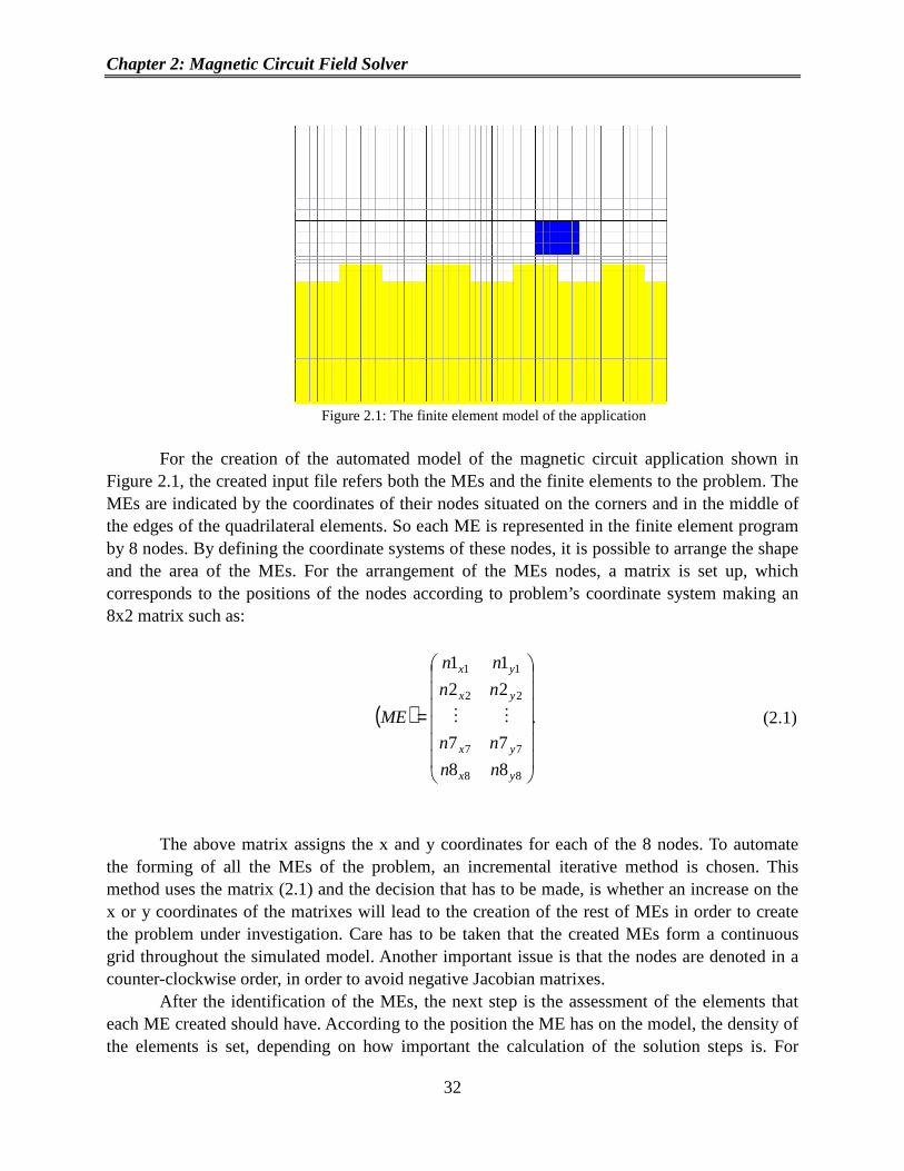
In Figure 2.1 the magnetic circuit application under investigation is demonstrated. Yellow denotes the gear wheel. Blue shows the magnetic structure, and white, the surrounding air. The bold lines depict the MEs, while the faint lines between the bold denote the finite elements.
Chapter 2: Magnetic Circuit Field Solver
32
Figure 2.1: The finite element model of the application
For the creation of the automated model of the magnetic circuit application shown in
Figure 2.1, the created input file refers both the MEs and the finite elements to the problem. The MEs are indicated by the coordinates of their nodes situated on the corners and in the middle of the edges of the quadrilateral elements. So each ME is represented in the finite element program by 8 nodes. By defining the coordinate systems of these nodes, it is possible to arrange the shape and the area of the MEs. For the arrangement of the MEs nodes, a matrix is set up, which corresponds to the positions of the nodes according to problem’s coordinate system making an 8x2 matrix such as:
( ) .
88
77
22
11
88
77
22
11
=
yx
yx
yx
yx
nn
nn
nn
nn
ME MM (2.1)
The above matrix assigns the x and y coordinates for each of the 8 nodes. To automate the forming of all the MEs of the problem, an incremental iterative method is chosen. This method uses the matrix (2.1) and the decision that has to be made, is whether an increase on the x or y coordinates of the matrixes will lead to the creation of the rest of MEs in order to create the problem under investigation. Care has to be taken that the created MEs form a continuous grid throughout the simulated model. Another important issue is that the nodes are denoted in a counter-clockwise order, in order to avoid negative Jacobian matrixes.
After the identification of the MEs, the next step is the assessment of the elements that each ME created should have. According to the position the ME has on the model, the density of the elements is set, depending on how important the calculation of the solution steps is. For

Chapter 2: Magnetic Circuit Field Solver
33
instance, along the MEs situated at the distance between the end of the magnet and the beginning of the gear tooth, the density of the elements creates a 6x4 matrix. This distance is the air gap distance of the magnetic circuit.
By default, the mesh which is chosen to solve this problem (Figure 2.1) is a mapped mesh. Map mesh is termed as the sequence of same shape, finite elements, creating the grid of the problem which can result in more accurate simulations, meaning that the simulated results are comparable with the experimental data. Moreover with mapped meshing, since fewer elements are required to model the problem, it also takes less time to be solved, in comparison with the free meshing.
2.2.2 Setting the boundaries of the problem For the creation of the automated model shown in Figure 2.1, it is also necessary to define the boundary conditions of the model. An input file is created that sets the constant boundary conditions on the lower edge of the meshed grid of Figure 2.1. Here the MEs that have their own edges tangential and in touch with the lower edge of the grid, are set to have the boundary’s values. For this selection, the edges are defined as Dirichlet boundary’s conditions and it is denoted that the magnetic field density takes place here, equal to Bnormal=0. Dirichlet simulations set a plane of symmetry in the problem. Therefore, by selecting the line on the lower edge of the problem to be under Dirichlet boundaries, the correct solution of the model is not affected. In the simplest case of simulating magnetic structures surrounded by air, where the field is to be calculated, the essential boundaries - as in the simulated model - as well as infinity boundaries are set. The infinity boundaries conditions are set on the four edges of the model. Those boundaries are far-field elements which approximate the decay of the magnetic field in the far-field region, since it is assumed that the magnetic field expands to infinity [61]. In this case, (magnetic circuit of Figure 2.1) in the presence of an iron gear wheel, where the magnet is placed nearby, since the relative permeability of the gear wheel is much higher than the relative permeability of the air, all the magnetic fluxes are accumulated in the iron wheel. This happens because the flux lines always follow the highest permeance route. Therefore, it is not necessary to use infinite elements.
2.2.3 Defining the material properties of the model
The material properties are given in a separate input file. This input file assigns material properties to the MEs. After that the pre-processing phase is completed and the model is ready for the solution. The file’s structure consists of, firstly, the declaration of the material’s properties; e.g. whether the material is isotropic or the magnet has a non linear second quadrant magnetization curve BH and so on. The next step is to set the relative permeability of the medium and finally to define the MEs which will be assigned to it. For instance, in the case of

Chapter 2: Magnetic Circuit Field Solver
34
air, the material property is isotropic material. The relative permeability of air is 1, followed by the number of MEs comprises the aerial space. For the case of a permanent magnet, the relative permeability, the magnetization directions as well as the BH curve of the magnet are asserted. By importing the magnetic material data, which includes the magnetic induction B and the corresponding magnetic field H it is possible to create the BH curve and attach it to the magnetic materials. It will be shown how the BH data can be imported to the automated model in section 2.4. An important issue is to simulate the movement of the magnetic circuit application of Figure 2.1. To investigate this movement and calculate the field distribution, another approach had been followed. It is known that the finite element grid discretizes the geometry of the problem in well specified and dimensioned small regions, the elements. Once defined, the elements cannot be moved nor changed inside the finite model. Therefore, the movement of the gear in front of the magnet or the movement of the magnet in front of the gear wheel is simulated using an indirect method. Several such different techniques to imitate the movement in the finite element modeling have been examined and presented [61] – [64].
As discussed before, the position of the magnet in the material input file is denoted by assigning the corresponding MEs to the magnetic material properties. By simultaneously creating material properties input files where the magnet properties are attached to the adjacent MEs, it is possible to imitate the movement of the magnet. This can happen within a loop where for each ME with appointed magnetic properties, the input material file is created. This input file along with the other input files; which are created in the pre-processing sector, are executed and the results are saved. Thereafter, a new material input file is created which assigns in a new ME, the magnetic material properties and then the operation is continued.
2.3 Post-processing section - Visualization of the results When the above input files are executed, the solution of the simulated model as it is shown in Figure 2.1 emerges. Following the solution of the automated program, comes the visualization of the calculated results. In the case of the circuit application of Figure 2.1, of most importance is the field distribution on the surface of the sensing element, in this case GMR elements. The magnetic sensor is situated below the magnet, and in front of the gear wheel. Since it does not affect the field it is omitted from the simulation model. To calculate the field distribution on the surface of the GMR elements, a post-processing file is created to visualize the field.
For the case of the static simulations, the model consists of the magnet surrounded by air. These simulations can give an indication on whether the magnetic field intensity can drive the GMR elements in saturation or not. The post-processing file which was created indicates the type of the process of the simulated results, which is to show the field distribution. Since the magnetic sensor is placed below the magnet and the distance of the GMR elements is known, depending on which MEs were set with their corresponding magnetic material properties, the post-

Chapter 2: Magnetic Circuit Field Solver
35
processing file provides the x and y coordinates of the path where the GMR elements are set. In this path and in a number of intermediate points of it, the magnetic field is to be calculated and stored for the visualization of the results. The coordinates are measured from the central coordinate system of the problem. Figure 2.2 demonstrates the in-plane (Bx) field distribution of a rectangular magnet. The field is calculated from one side of the magnet to the other in a distance 0.3 mm below the magnet. It is assumed that the sensor is attached to the magnet and therefore the normal distance of the GMR elements to the end face of the magnet is 0.3 mm.
Figure 2.2: In-plane field distribution for a static simulation of a rectangular magnet
In the case of movement, each step of the magnet is denoted with the help of a loop
action. Therefore, for every step of the magnet, a post-processing file is created and attached to the corresponding magnetic material MEs. Once the solution has been found, the results created from the post-processing file are stored. Thereafter a new post-processing file is created, setting the new coordinates of the calculation path, according to the next position of the magnet, as it is described in the new material properties input file. By the end of the sequence, for each of the positions of the MEs enhanced with the magnetic properties, the calculated results are stored and compiled to give the field distribution along the movement of the magnet.
2.4 Automation of the model, introducing the GUI of the model The automated model is based on the above four files described. The input files create the finite model under investigation and set the boundaries conditions of the model. Likewise, at the material input file, the material properties of the model are appointed to the corresponding MEs of the model. The post-processing file has been created to visualize the field distribution on a selected path direction. For the automation of the simulation of the model based on the above created files, a method has to be introduced that helps the user to execute the problem with the
-1
-0.8
-0.6
-0.4
-0.2
0
0.2
0.4
0.6
0.8
1
33.5 34 34.5 35 35.5 36 36.5Bx
(mT
)
distance(mm)

Chapter 2: Magnetic Circuit Field Solver
only interferences being, introducing to the model, parameters under investigation, such as material properties or the air gap A GUI as it is shown in also developed in a MATLAB environment. For a magnetic circuit problem as in not only possible to simulate and get the magnetic field distribution on a path under investigation, but also to change crucial parameters and get new results. The magnetic material properties can be loaded from the GUI, in any file or the number of points of the second quadrant BH curve, it is possible to get the BH curve of the magnetic structure under investigation. The next step is to indicate the case it is measured from the ending side of the magnet until the starting point of the gear wheel tooth. The movement steps can be set to imitate the real movement of the gear wheel along the stationary part, back-bias magnet and magnetic sensor. The next step can be the swhether simulations can be static and show only the magnetic field distribution. Or if the selection is in rotation, to perform the movement simulations and get the change of the magnetic field while the magnet changes positions along the wheel
Figure 2.
By pressing the execution button (Start the Simulation), the three input files are created as well as taking into account the user’s input parameters. The Rotation Simulation wa simulation of the magnetic circuit application ofwill get the field distribution along a path with the help of the postand field distributions such as Figure 2.
Magnetic Circuit Field Solver
36
only interferences being, introducing to the model, parameters under investigation, such as air gap distance.
in Figure 2.3 has been created to automate the model. The GUI is MATLAB environment. For a magnetic circuit problem as in
not only possible to simulate and get the magnetic field distribution on a path under investigation, but also to change crucial parameters and get new results. The magnetic material properties can be loaded from the GUI, in any file or database format. With the material file and the number of points of the second quadrant BH curve, it is possible to get the BH curve of the magnetic structure under investigation. The next step is to indicate the air gap
ed from the ending side of the magnet until the starting point of the gear wheel tooth. The movement steps can be set to imitate the real movement of the gear wheel along the
bias magnet and magnetic sensor. The next step can be the swhether simulations can be static and show only the magnetic field distribution. Or if the selection is in rotation, to perform the movement simulations and get the change of the magnetic field while the magnet changes positions along the wheel.
Figure 2.3: The GUI of the automated model
By pressing the execution button (Start the Simulation), the three input files are created as well as taking into account the user’s input parameters. The Rotation Simulation wa simulation of the magnetic circuit application of Figure 2.1. Pressing the ‘get the results’ button will get the field distribution along a path with the help of the post-processing visualization file
Figure 2.2 are plotted.
only interferences being, introducing to the model, parameters under investigation, such as
the model. The GUI is MATLAB environment. For a magnetic circuit problem as in Figure 2.1, it is
not only possible to simulate and get the magnetic field distribution on a path under investigation, but also to change crucial parameters and get new results. The magnetic material
database format. With the material file and the number of points of the second quadrant BH curve, it is possible to get the BH curve of the
air gap distance; in this ed from the ending side of the magnet until the starting point of the gear wheel
tooth. The movement steps can be set to imitate the real movement of the gear wheel along the bias magnet and magnetic sensor. The next step can be the selection of
whether simulations can be static and show only the magnetic field distribution. Or if the selection is in rotation, to perform the movement simulations and get the change of the magnetic
By pressing the execution button (Start the Simulation), the three input files are created as well as taking into account the user’s input parameters. The Rotation Simulation will perform
. Pressing the ‘get the results’ button processing visualization file

Chapter 2: Magnetic Circuit Field Solver
37
2.5 Conclusion
An automated field simulator is presented and the way it has been created is explained. The automated model is based on the Finite Element Model simulator EleFAnT2D, to be executed. For this reason input files are created, which are responsible for introducing the geometry of the problem and its discretization. Another input file is responsible for attaching the material properties with the corresponding MEs of the problem. The boundary’s conditions of the problem are created in the last input file. For the visualization of the results a post-processing file has been created, which detects the position of the magnetic sensing elements and calculates the field distribution along that path. Finally a GUI interface is introduced, which combines the above files with the solve section of the EleFAnT model and which automates the finite element simulations.
The benefit of such a model is that the end-user does not need to take into consideration how to perform the simulations. Only by changing crucial parameters under investigation, is it possible to calculate the field results and to test the magnetic sensor functionality in the specified magnetic circuit described by the model. Moreover, the program has the benefit of being very fast in terms of computational time and does not need huge hardware resources.

Chapter 3: Investigations of Angular Magnetic Sensors with field-splitter layer
38
3 Investigations of Angular Magnetic Sensors with field-splitter layer
Investigations of the proposed GMR angular sensor configuration are presented. A magnetic field controlling layer is introduced to overcome the problems of angular sensor working conditions. Section 3.1 provides a brief description and the origin of the problem. The proposed model under investigation is presented in section 3.2. The investigations were carried out in two dimensions. The following section 3.3 details the simulated model and the respective analysis. Finally, in section 3.4 the parametric model results are discussed and the optimum field splitter layer solution is identified.
3.1 Description of the problem
The angle magnetic sensor is used to determine the rotation angle over a range of 360° degrees. In the case of GMR angular sensors, the elements are arranged in two Wheatstone bridges. Under a rotated external field, the two bridges generate a cosine and a sine signal output whose arc-tangent derives the output sensor signal.
GMR elements have a high sensitivity and they can detect low magnetic fields. Although they are used for contactless measurements, they have a drawback. They have a rather small operating magnetic window in comparison with other sensor techniques such as Hall-effect. According to the distance of the sensor to the magnetic source, the operating range is determined by:
.maxmin HHH operate⟨⟨ (3.1)
If the external magnetic field is too large, GMR properties are changed, causing an error output magnetic sensor signal. If the external field is too small, the soft magnetic sensing layer or free

Chapter 3: Investigations of Angular Magnetic Sensors with field-splitter layer
39
ferromagnetic layer does not reach saturation and the resulting signal will reveal hysteresis effects along the 360°degrees rotation, causing significant angle errors. Furthermore, sensors might be exposed to other external magnetic fields, which can overlap and thus lead to an error angular output. Additionally it has to be mentioned that for the angular sensor applications, the GMR elements must work in their saturation mode, where the magnetization directions of target and free layer are antiparallel, revealing maximum resistance. In order to determine the optimum working conditions of the sensor, the external magnetic field should be monitored permanently. To overcome sensor mis-functions, an added split field arrangement placed on the top or at the bottom of the GMR element is proposed which can solve the problems mentioned above. Additional ferromagnetic layers could split the magnetic flux and thus keep magnetic sensors on their operating range.
3.2 Investigation of the 2D problem
The general idea of the concept is depicted in Figure 3.1: Scheme of the proposed concept. As it can be seen the proposed field control layer splits the field distribution reducing the field strength which is measured by the GMR element.
Figure 3.1: Scheme of the proposed concept
The stack consists of two SiO2 layers with a height of 500 nm. In between is the ferromagnetic material Co90Fe10. A second ferromagnetic layer, Co90Fe10, with a height of 10 nm serves as a protection layer between the stack and the substrate beneath the three layers. Co90Fe10 is a ferromagnetic material. By Bozorth's the maximum permeability of Co90Fe10 is 4,000 [65]. A bar magnet with a length of 5 mm and a height of 1 mm was chosen as a magnetic source. The air gap between the magnet and the stack is 800 µm. A scheme of the model can be seen in Figure 3.2.

Chapter 3: Investigations of Angular Magnetic Sensors with field-splitter layer
40
Permanent magnet
5 mm
1 mm
Si wafer
1.7 mm
600 um
SiO2
SiO2
CoFe
600 um
CoFe 2layer
SiO2500 nm
500 nm
Y distance (nm)
10 nm
10 nm
800 um
Y
Figure 3.2: Split-field geometry under investigation
The permanent magnet, which is perpendicular, has a length of 5 mm and a height of 1 mm. An Alnico 700T magnet was used for this application. The demagnetization curve of the Alnico 700T magnet is shown in the following Figure 3.3:
-60 -50 -40 -30 -20 -10 00
200
400
600
800
1000
1200
1400
B(m
T)
H(kA/m)
demagnetization curve of Alnico 700T
Figure 3.3: Demagnetization curve of the Alnico 700T magnet
A swift estimation of the magnetic field intensity on the surface of the layer, which will
be created by an Alnico 700T magnet with the dimensions 5 x 1 x 5 mm can be found with the aid of a magnetic charge model. A bar magnet, as can be seen in Figure 3.4, is being assumed. The magnet has the following dimensions: xmag width, ymag depth, and zmag height. Likewise it was assumed that the magnetization direction is normal:

Chapter 3: Investigations of Angular Magnetic Sensors with field-splitter layer
41
M zMˆ= . (3.1) The magnetic charge model is an analytical method used to calculate the Bz field
distribution [66]. The charge model method replaces the magnet structure with a distribution of “magnetic charges,” proportional to the electric charges. Using the charge model, the “magnetic charges” are placed on the area along the z-axis, as can be seen in Figure 3.4:
Figure 3.4: Equivalent charge model
Magnetic charges are defined by means of the equations 3.2 and equation 3.3, which
describe the distributions of the charge densities:
•−∇=mρ M Volume charge density (3.2)
=mσ M n• Surface charge density (3.3)
Assuming that all the “magnetic charges” settle on the +z and –z surface of the magnet
(see Figure 3.4), the volume charge density is zero. The surface charge density is:
.Sm M±=σ (3.4)
The magnetic field of a magnet with the magnetization direction in free space is
given by the following equation:
( ) ( )( ) ( )( ).
44 30
30 ∫∫ ′
′−
′−′+′
′−
′−′= sd
xx
xxxvd
xx
xxxxB mm σ
πµρ
πµ
(3.5)
In the point x the field is calculated, x′ is the source point. In the configuration shown in
Figure 3.4, the investigated point is on the z-axis, zzx)= , and x′ is located at the XY plane (
yyxxx magmag ˆˆ +=′ ). By substituting the assumptions in equation 3.5 and taking into account
equation 3.4, the following equation is obtained:

Chapter 3: Investigations of Angular Magnetic Sensors with field-splitter layer
42
( ) ( ) .4
0 0
2/3222
0 ∫ ∫ ′′′+′+′
=mag magx y
Sz ydxd
zyx
zMzB
πµ
(3.6)
Finally, the Bz field distribution in a point z on the z-axis can be calculated with the
equation:
( ) ( )
++−
++++= −−
magmag
magmag
magmag
magmagmagmagsz yx
zyxz
yx
zzyxzzMB
2221
22210 tantan
πµ
Where magx , magy and magz denote the dimensions of the magnet. It can be concluded that Bz is
approximately 60 (mT) at z = 0.8 mm.
3.3 Simulated model and parametric analysis
The simulated model is illustrated in Figure 3.5. The model consists of the bar magnet and the surrounding air. The far boundary (surrounding air) is at a distance of 5 times the dimensions of the magnet. If the air region is too small, the field distribution will be distorted, which leads to significant errors. If it is too large, the calculation time is increased.
Figure 3.5: Model under investigation

Chapter 3: Investigations of Angular Magnetic Sensors with field-splitter layer
43
The model has approximately 4.000 elements using 2D 8-node isoparametric elements based on magnetic vector potential formulation. The effects of the far-field decay of the magnetic field for this open boundary problem were modeled using infinite elements. Infinite elements assume that the degree of freedom (DoF), in this case magnetic vector potential, at infinity is zero. The overall estimated calculated time is less than a minute. The resulting magnetic field lines can be seen in Figure 3.6. The red circle on the outer surface is symbolizing the far-field approximation.
Figure 3.6: Magnetic flux density distribution
For the investigations, the first ferromagnetic layer, FeCo, (as it can be seen in the field
split layer of Figure 3.2) had a constant height of 10 nm. The second layer, the one in the vicinity of the magnetic structure, is altered in height. The heights are 6, 11, 24 and 48 nm.
3.4 Results and conclusions
The magnetic flux was calculated for both ferromagnetic layers. While the height of the first layer did not change, the height of the other layer varied. The flux is calculated by the equation:
,∫=Φ BdS (3.7)

Chapter 3: Investigations of Angular Magnetic Sensors with field-splitter layer
44
where S is the height of the layers per unit depth of their surface. The results are listed in the following Table 3.1:
layers magnetic flux Φ
(Weber/mm) 1st FeCo (10 nm) 4.79E-4 2nd FeCo (6 nm) 2.98E-4
1st FeCo (10 nm) 4.97E-4 2nd FeCo (11 nm) 5.44E-4
1st FeCo (10 nm) 5.34E-4 2nd FeCo 24 nm) 1.2E-3
1st FeCo (10 nm) 4.32E-4 2nd FeCo (48 nm) 2.4E-3
Table 3.1: Results for the magnetic fluxes
The results show that it does not make a real difference whether a 6 or an 11 nm Co90Fe10
layer is used. Yet, there is a difference between a 24 nm and a 48 nm layer. Using a second ferromagnetic layer with a height of 48 nm definitely is the best solution.
3.5 Conclusion
A proposed field control layer was introduced and investigated [67]. This layer consists of a series of ferromagnetic and antiferromagnetic layers which can be situated on the top of the GMR elements. The same results can be found if the split-layer is placed at the bottom of the GMR stack. Four different cases of ferromagnetic layer heights were simulated. It could be determined that a ferromagnetic layer with a maximum height of 48 nm is the best solution. Such a layer offers the possibility to split the flux impacting the sensor and to keep the field passing through the GMR elements inside their magnetic field intensity operating window.
For the investigations, a 2D FEM model was created to calculate the magnetic flux passing through each layer.

Chapter 4: Investigation of back-bias magnets
45
4 Investigation of back bias magnets
Investigations of magnetic structures and material properties are presented in this chapter. The magnets were simulated to calculate the magnetic field intensity that the GMR elements are sensing. The correct choice of the back bias magnets is crucial for the correct function of the GMR sensors. Section 4.1 will give an insight in the problem under investigation. In Section 4.2 the 3D simulated model is described as well as the optimization process which follows to get the desired magnetic field intensity on the surface of the GMR elements. Section 4.3 describes the U-shape magnetic structures whereas section 4.4 shows the field distribution of bar magnets. Section 4.5 refers to an inverse problem, where the magnetic structure geometries are known and they are optimized to get the desired magnetic circuit application. In section 4.6 the investigations regarding the iBB magnet are explored, which presents numerous benefits in applications. Finally section 4.7 shows the calculations of the magnetization angles of the GMR elements along their surface when they are influenced by an external magnetic field.
4.1 Description of the problem
Magnetic circuits play a crucial role in automotive technology. The magnet, which serves as the source of the circuit, is called the back bias magnet. It is the active part of the circuit, while the gear wheel is its passive part. Due to the high sensitivity of GMR elements, saturation has to be avoided by all means. Hence, a proper selection of the back bias magnet is essential for the correct operation of the magnetic sensors. Back bias magnets must guarantee linearity and a homogeneous field distribution on the surface of GMR stacks. Therefore, it is critical to investigate and optimize not only the shape of the magnet but also the magnetization’s strength and direction. Magnets can be realized in different shapes. Furthermore, magnets can be replaced by a magnetic encoder wheel.
In order to evaluate the performance of back bias magnets, finite element methods can be used. Of particular interest is the plane field distribution on the surface of the GMR elements.

Chapter 4: Investigation of back-bias magnets
46
Moreover, it has to be investigated whether GMR elements are in their working range or if they reach saturation. In addition, it is of particular importance to investigate the normal direction of the magnetic field distribution in order to have an indication of the air gap performance. Therefore, the investigations have to be carried out in 3D. These simulations can provide an overview of the suitability of magnets.
4.2 3D simulated model
For the investigation of back bias magnets, the simulation of the field distribution and the calculation of the field intensity in three dimensions should be a first approximation. More precise results can be obtained by simulating the magnets in their application environment to determine their suitability. However, these static 3D simulations are an inexpensive way to verify the proper selection of the structure of the magnet. Since the magnetization direction of the free layer of the GMR elements follows the magnetization direction of the field on the surface of the element, the simplified simulated model consists of the magnet structure and the surrounding air. The measurement of the field distribution is the output of the simulations on the surface of the GMR elements.
Figure 4.1: Path calculation of the field distribution along the GMR stripes
Moreover, the normal field intensity is investigated. These investigations can give an
estimation of the air gap performance of the magnet in automotive applications. The calculation of the field distribution is performed along a path along the GMR stacks. Figure 4.1 shows the front view of a magnetic sensor. The four GMR elements of the Wheatstone bridge are situated on the two edges of the chip, while the fifth element, which calculates the position, is placed at the center of the chip. The path simulation of the field is at the center of the GMR elements.

Chapter 4: Investigation of back
To create the model, a solid 3magnetic structure and the surrounding airapproach was used and the modelwell formed, material properties model was meshed. The 2D model problem, infinity elements weredecay due to the distance from the magnetic source.
Attention has to be paid to the proper connectivity of the 3D modelshows the discontinuity of the model, which is a typical problem.
Figure 4.2a shows the problem of discontinuity. Magnetic field fluxes mainly have the
tendency to exit the magnet through the corners of the structure as indicated by the Laplace
equation 02 =∇ ϕ . As can be seen in
not in the corner areas of the magnetic structure. If the model is investigated more carefully, it can be seen that the aerial elements, which are shaelements associated with the magnet (magentaand the magnet geometry (see partially connected with the magnetic elements (magenta colored).Neuman boundary conditions between the elements describing the magnetic material and the elements describing the air. This uncoupled model wicalculations. Besides the investigations and simulations of the geometry of the magnet, to get an optimumelements is another important issueoptimization is the following:
Figure 4.2a: Magnetic potential on the surface of the magnetof the model
Investigation of back-bias magnets
47
el, a solid 3D magnetic scalar potential element is used to simulate the e and the surrounding air. This element consists of 20 nodes
the model was first created in 2D. With this approachwell formed, material properties were associated with the corresponding 2D geometry and the
D model was then extruded to 3D. Since it is an open boundarwere performed at the edge of the model, to approximate
distance from the magnetic source. Attention has to be paid to the proper connectivity of the 3D model in ANSYS
shows the discontinuity of the model, which is a typical problem.
shows the problem of discontinuity. Magnetic field fluxes mainly have the tendency to exit the magnet through the corners of the structure as indicated by the Laplace
seen in Figure 4.2a, the maximum and minimum field strength is
not in the corner areas of the magnetic structure. If the model is investigated more carefully, it can be seen that the aerial elements, which are shaded green, are not correctly connected to the elements associated with the magnet (magenta-colored) at the surface interface between the air and the magnet geometry (see Figure 4.2b).The 3D aerial elements (green c
connected with the magnetic elements (magenta colored). This is due to discontinuity of Neuman boundary conditions between the elements describing the magnetic material and the
This uncoupled model will lead to false field distribution
the investigations and simulations of the magnet structure, the optimizto get an optimum magnetization intensity on the surface of GMR
tant issue. A pseudo-algorithm which shows the process of the
: Magnetic potential on the surface of the magnet Figure 4.2b: Discontinuity
used to simulate the nodes. A bottom-up
D. With this approach, the model was D geometry and the
Since it is an open boundary , to approximate the field
in ANSYS. Figure 4.2
shows the problem of discontinuity. Magnetic field fluxes mainly have the tendency to exit the magnet through the corners of the structure as indicated by the Laplace
the maximum and minimum field strength is
not in the corner areas of the magnetic structure. If the model is investigated more carefully, it ded green, are not correctly connected to the
colored) at the surface interface between the air The 3D aerial elements (green colored) are only
This is due to discontinuity of Neuman boundary conditions between the elements describing the magnetic material and the
ll lead to false field distribution
, the optimization of on the surface of GMR
the process of the
4.2b: Discontinuity

Chapter 4: Investigation of back-bias magnets
48
program optimize backBias_magnet implicit none ! declare design variables real::i,magx,magy,magz,Mstr,Bmax real::magxN,magyN,magzN read(*,*)Bmax ! initial calculations write(10,*)magx,magy,magz,Mstr !perform the FEM simulations do (magx,magy,magz,Mstr),i,(magx,magy,magz,Mstr)MAX
open(10,file=’results from FEM simulations’Bfield.out ) read(10,*)Bfield if(Bfield.le.Bmax) then
write(*,*)’ Optimization has been performed successfully’ close(10)
else magxN=magx+i magyN=magy+i magzN=magz+i write(10,*)magxN,magyN,magzN !continue FEM simulations with the new design variables end if end do stop end program optimize backBias_magnet
Using the 3D simulations, the field intensity in the center of the GMR element is calculated. This is the objective function whose value must meet the specifications. The quantities that are varied to achieve the optimum design are the geometry dimensions of the magnet and/or the magnetization of the magnet. The objective function is calculated for the initial values of the design variables. A loop starts if the value does not meet the expectations. Figure 4.3 shows the optimization procedure in a flowchart form.

Chapter 4: Investigation of back
Change Design-Variables
according to specifications
Figure 4.
4.3 Investigation of U-shaped magnets
U-shaped magnets are widely is influenced by the gap dimension of the Udemagnetization, curve and a remanence of Bcontour plot of the magnetic field distribution on the surface of the magnet. A magnetic sensor can be placed in the center of the GMR elements is located beneath the edge of the magnet. This can be seen
Figure 4.4a: Contour B plot of the U-
Investigation of back-bias magnets
49
inputEMAG
FEM model
Calculate Bx field @ the center of GMR element
END
according to specifications
mTBx 2≤
START
Calculation of field distributionon the surface of GMR
elements
Figure 4.3: Flowchart of the optimization procedure
shaped magnets
shaped magnets are widely spread in magnetic applications [68]. The field distribution d by the gap dimension of the U-shape. A neodium magnet
and a remanence of Br = 287 mT was used. Figure 4.magnetic field distribution on the surface of the magnet. A magnetic sensor
can be placed in the center of the U-shaped magnet so that each of the half Wheatstone bridge beneath the edge of the magnet. This can be seen in Figure 4.
-shaped magnet Figure 4.4b: U-shaped back bias magnet and MS structure
. The field distribution magnet, with linear
Figure 4.4a shows the magnetic field distribution on the surface of the magnet. A magnetic sensor
Wheatstone bridge Figure 4.4b.
shaped back bias magnet and MS

Chapter 4: Investigation of back
Magnetic field distributions in the x and y direction at a distance of poles of the U-shaped magnet are shown in
Figure 4.5a: Bx field distribution
Four geometries have been investigatdimensions of the magnetic structure were the samechanged every time from a larger gap dimension to a smaller one. The four different cases can be seen in Figure 4.6:
Figure 4.
The first geometry has a deep and wide gap whereas the 3
narrower gap. The other two geometries hcomponents of the magnet beneath the poles
3rd geometry3rd geometry
Investigation of back-bias magnets
50
Magnetic field distributions in the x and y direction at a distance of 0.5 mm below the shaped magnet are shown in Figure 4.5:
field distribution Figure 4.5b: By field distribution
Four geometries have been investigated further and are of most interest. The x, y and z agnetic structure were the same and the x and y dimensions of the gap
changed every time from a larger gap dimension to a smaller one. The four different cases can be
Figure 4.6: Different U-shaped magnet geometries
geometry has a deep and wide gap whereas the 3rd geometry has also a deep but narrower gap. The other two geometries have a shorter gap length. Figure 4.
of the magnet beneath the poles along the side of the magnet.
1st geometry 2nd geometry
3rd geometry 4tht geometry
1st geometry 2nd geometry
3rd geometry 4tht geometry
0.5 mm below the
field distribution
and are of most interest. The x, y and z and the x and y dimensions of the gap
changed every time from a larger gap dimension to a smaller one. The four different cases can be
geometry has also a deep but Figure 4.7 show the field

Chapter 4: Investigation of back-bias magnets
51
Figure 4.7a: Magnetic field distribution in the x-direction Figure 4.7b: Magnetic field distribution in the y-direction
Figure 4.7c: Magnetic field distribution in the z-direction
When decreasing the gap dimensions, the magnetic field intensity decreases. Especially
the x and y component of the field distribution are influenced by the reduction of the U-structure. This is usable for the GMR elements since these field distributions influence their working status.
Figure 4.8a: Magnetic field distribution in the x-
direction Figure 4. 8b: Magnetic field distribution in the y-
direction
-0.001 0.000 0.001 0.002 0.003 0.004 0.005 0.006 0.007 0.008-1.0x10
-1
-8.0x10⁻²
-6.0x10⁻²
-4.0x10⁻²
-2.0x10⁻²
0.0
2.0x10⁻²
4.0x10⁻²
6.0x10⁻²
8.0x10⁻²
Bx(
T)
distance(m)
Bx-1st geometry Bx-2nd geometry Bx-3rd geometry bx-4th geometry
-0.001 0.000 0.001 0.002 0.003 0.004 0.005 0.006 0.007 0.008-0.12
-0.10
-0.08
-0.06
-0.04
-0.02
By(
T)
distance(m)
By-1st geometry By-2nd geometry By-3rd geometry by-4th geomety
-0.001 0.000 0.001 0.002 0.003 0.004 0.005 0.006 0.007 0.008-4.5x10⁻⁷
-4.5x10⁻⁷
-4.5x10⁻⁷
-4.4x10⁻⁷
-4.3x10⁻⁷
-4.3x10⁻⁷
-4.3x10⁻⁷
-4.2x10⁻⁷
-4.1x10⁻⁷
-4.1x10⁻⁷
-4.0x10⁻⁷
-4.0x10⁻⁷
Bz(
T)
distance(m)
Bz-1st geometry Bz-2nd geometry Bz-3rd geometry bz-4th geometry
-0.001 0.000 0.001 0.002 0.003 0.004 0.005 0.006 0.007 0.008-0.005
0.000
0.005
0.010
0.015
0.020
0.025
Bx(
T)
distance(m)
Bx-1st geometry bx-2nd geometry Bx-3rd geometry bx-4th geometry
-0.001 0.000 0.001 0.002 0.003 0.004 0.005 0.006 0.007 0.008-0.11
-0.10
-0.09
-0.08
-0.07
-0.06
-0.05
-0.04
-0.03
-0.02
By(
T)
distance(m)
By-1st geometry by-2nd geometry By-3rd geometry by-4th geometry

Chapter 4: Investigation of back-bias magnets
52
The investigation of the plane magnetic field on the surface of the GMR elements is another important issue. The simulation results indicate where to place the magnetic sensor so that the GMR elements can measure a homogeneous magnetic field without reaching saturation. Figure 4.8 demonstrate the magnetic field distribution along the edge of the magnet in the direction of the left half bridge GMR element at a distance of 0.5 mm below the magnet.
Of the four simulated geometries above, the last one (4th geometry) with a thinner and shorter gap dimension appears to produce better results. When decreasing the gap of the U-shaped magnet, the field distribution becomes smaller on the surface of the GMR element, thus avoiding a saturation of the elements. Moreover, the plane field distribution on the GMR surface is homogeneously distributed. The x and y field distribution along the GMR surface have a constant value. This can be seen in Figure 4.8a and Figure 4.8b. It is assumed that the GMR elements are situated in the middle of the magnet’s face. Thus, for the GMR magnetic sensor applications, the best performance can be achieved when using a U-shaped magnet with a shallow gap as a magnetic circuit source.
4.4 Investigation of bar magnets
The bar magnet structure which can produce sufficient results, is an important magnet geometry. Various bar shaped magnets have been simulated and their magnetic field distributions have been calculated for various magnetization directions. The advantage of bar magnets is their homogeneous magnetic field distribution and the low cost of production. The contour plot of the magnetic field of a bar magnet with the dimension 8 x 4 x 8 mm and a normal magnetization direction is illustrated in Figure 4.9.
Figure 4.9: Contour B plot of a bar magnet
Figure 4.10 illustrates the magnetic field distribution in the normal (y-axis) and projected
direction (x-axis) for various geometries. The dimensions of the magnets under investigation are 10 x 4 x 10 mm (first geometry), 8 x 8 x 8 mm (second geometry), and 7 x 7 x 7 mm (third geometry). The magnetization direction lies in the normal direction.

Chapter 4: Investigation of back-bias magnets
53
Figure 4. 10a: Magnetic field distribution in the x
direction Figure 4. 10b: Magnetic field distribution in the y
direction
A magnetic structure with thinner dimensions in the normal direction (in this case in the y direction) produces a weaker magnetic field strength as can be seen in the field distribution of the first geometry. The other two geometry distributions reveal that the field intensity produced is not very different. The third geometry might be the most suitable one for an application due to cost reasons. As the GMR elements reach saturation very easily, the first geometry (10 x 4 x 10 mm) is the most convenient of the three geometries.
The magnetic field distribution on the surface of the GMR elements for the first geometry can be seen in Figure 4.11. The figure shows the magnetic field distribution along the edge of the magnet in the direction where the left half bridge GMR elements are placed. It was assumed that the magnetic sensor has been placed at the center of the magnet and 0.5 mm beneath it. The results show the homogeneity of the field distribution along the surface of the GMR elements.
Figure 4. 11a: Magnetic field distribution in the x-
direction Figure 4. 11b: Magnetic field distribution in the y-
direction
The best position of the GMR magnetic sensor is at the center beneath the magnet as it can be assured that the plane field distribution along the surface area of the elements is stable and homogeneous. Unfortunately, due to packaging tolerance reasons, the position of the sensor may fluctuate. For the first bar magnet geometry, there are four different scenarios for where the sensor can be placed beneath the back bias magnet (Figure 4.12a). In the figure, the dots symbolize the left and right GMR half Wheatstone bridge. The first scenario shows the best
0,0 2,0x10 -3 4,0x10⁻³ 6,0x10⁻³ 8,0x10 -3 1,0x10⁻²
-0,10
-0,08
-0,06
-0,04
-0,02
0,00
0,02
0,04
0,06
0,08
0,10
Bx(
T)
distance(m)
Bx-1st geometry Bx-2nd geometry Bx-3rd geometry
0,0 2,0x10- 3
4,0x10⁻³
6,0x10- 3
8,0x10⁻³
1,0x10⁻²
-0,11
-0,10
-0,09
-0,08
-0,07
-0,06
-0,05
-0,04
-0,03
By(
T)
distance(m)
By-1st geometry By-2nd geometry By-3rd geometry
0, 0 2,0x1 0-3 4, 0x10 -3 6,0 x10- 3 8 ,0x1 0-3 1, 0x10 -2
-9,5 x10 -3
-9,0 x10 -3
-8,5 x10⁻³
-8,0 x10⁻³
-7,5 x10 -3
-7,0 x10 -3
-6,5 x10 -3
-6,0 x10⁻³
-5,5 x10⁻³
-5,0 x10 -3
Bx(
T)
distance(m)
Bx dis tribution
0,000 0,00 2 0,0 04 0,006 0,008 0,010
-8,0x10⁻²
-7,0x10⁻²
-6,0x10 -2
-5,0x10 -2
-4,0x10⁻²
-3,0x10⁻²
-2,0x10 -2
By(
T)
distance(m)
By distribution

Chapter 4: Investigation of back-bias magnets
54
position in the case where the sensor is located beneath the magnet and symmetrically to the center of the magnet.
Figure 4.12a: Four different positions of the
investigated MS Figure 4. 12b: Four different positions of the
investigated MS
The in-plane (Bx) distribution on the surface of the left GMR half Wheatstone bridge can be seen in Figure 4.12b. When inspecting the field distributions, it can be stated that the GMR bridges move towards their initial symmetrical position and the field strength increases, driving them to the saturation mode of the elements.
4.5 Investigation and optimization of different magnetic structures
When using GMR sensors in magnetic applications, the back bias magnet is usually not attached to the sensor since the GMR elements reach saturation easily. Keeping a distance to the magnet can assure that the sensor is in a working condition. Thus, it is very challenging to design applications in which the back bias magnet is connected directly to the sensor. Such applications have to guarantee not only that the GMR elements will work in their operating window but also that the magnetic sensors will achieve a high air gap performance.
4.5.1 Investigated initial geometries Various designs of magnetic structures have been simulated. Such geometries can be seen in Figure 4.13.
0,0 2,0x10⁻³
4,0x10⁻³
6,0x10⁻³
8,0x10⁻³
1,0x10⁻²
-1,0x10⁻²
-8,0x10⁻³
-6,0x10⁻³
-4,0x10⁻³
-2,0x10⁻³
0,0
2,0x10⁻³
4,0x10⁻³
6,0x10⁻³
Bx(
T)
distance(m)
bx-scenario1 bx-scenario2 bx-scenario3 B-scenario4

Chapter 4: Investigation of back-bias magnets
55
x
y
z
Figure 4.13a: Joint pole Figure 4.13b: Angled magnet
x
y
z
Figure 4.13c: Cone magnet Figure 4.13d: Two-tilted magnet structure
Figure 4.13e: Bar magnet with V-iron plate
A typical air gap performance of magnetic sensors, based on the Hall Effect phenomenon, is approximately 4 mm. For comparison reasons the GMR sensors should have similar working conditions. The target of the air gap functionality is at least 4 mm in this case. Consequently, a strong SmCo magnet with a remanence of BR = 1.12 T and coercive force of HC = 780 (kA/m) was used to ensure that the application is working properly within the air gap specifications.
Since the sensor is attached to the magnet and the GMR elements reach saturation easily, optimization investigations of the geometries shown in Figure 4.13 assured the desired working capabilities. In Figure 4.13a, the joint pole magnet structure consists of two bar magnets with a normal magnetization and separated by an iron pole piece. Figure 4.13b shows a bar magnet with a magnetization direction tilted on the yz area. The magnetization is making an angle with the

Chapter 4: Investigation of back-bias magnets
56
normal direction (z-axis). Figure 4.13d shows two bar magnets connected to each other with their magnetization directions is laid on the xz area, making an angle with the normal direction (z-axis). The other two structures have cone geometry (see Figure 4.13c) and a V-iron plate attached to a bar magnet (see Figure 4.13e) trying to imitate the U-shaped magnet field distribution.
4.5.2 Simulation results of magnetic structures
The simulated results of the magnetic structures mentioned above in Figure 4.13 are presented below:
4.5.2.1 A. Joint pole
The Joint Pole structure consists of two bar magnets separated by an iron plate. Two
different geometries have been investigated. Their field distributions can be seen in Figure 4.14. The first one consists of two small magnets with the dimensions 2 x 1 x 2 mm, separated by an iron plate with the dimensions 0.2 x 1 x 2 mm. The second was made of two big magnets with the dimensions 6 x 2.5 x 4 mm, separated by an iron plate with the dimensions 0.4 x 2.5 x 4 mm.
-0.5 0.0 0.5 1.0 1.5 2.0 2.5 3.0 3.5 4.0 4.5 5.0 5.5-160
-140
-120
-100
-80
-60
-40
-20
0
Bx(
mT
)
distance(mm)
1 sc 2 sc
-0.5 0.0 0.5 1.0 1.5 2.0 2.5 3.0 3.5 4.0 4.5 5.0 5.5
-30
-20
-10
0
10
20
30
By(
mT
)
distance(mm)
1 sc 2 sc
Figure 4.14 a: Bx field distribution Figure 4.14b: By field distribution
The Bx and By distribution were measured in a path along the magnet where the left half
bridge GMR element is placed. Smaller geometries showed good results around the critical working field strength of the GMR elements. Therefore, the proposed structure is a suitable candidate to cover the specifications.
Another suitable approach could be the use of a smaller iron plate. Figure 4.15 depicts the field distribution on a path along the magnetic structure for geometries of magnets with the dimensions 2.2 x 5.8 x 7.5 mm and an iron plate with the dimensions 0.5 x 5.8 x 6.7 mm. As the GMR elements are placed at the center of the magnetic structure face, the plane field distribution on the surface of the elements is small. On the basis of an optimization process, these elements can be a practicable solution.
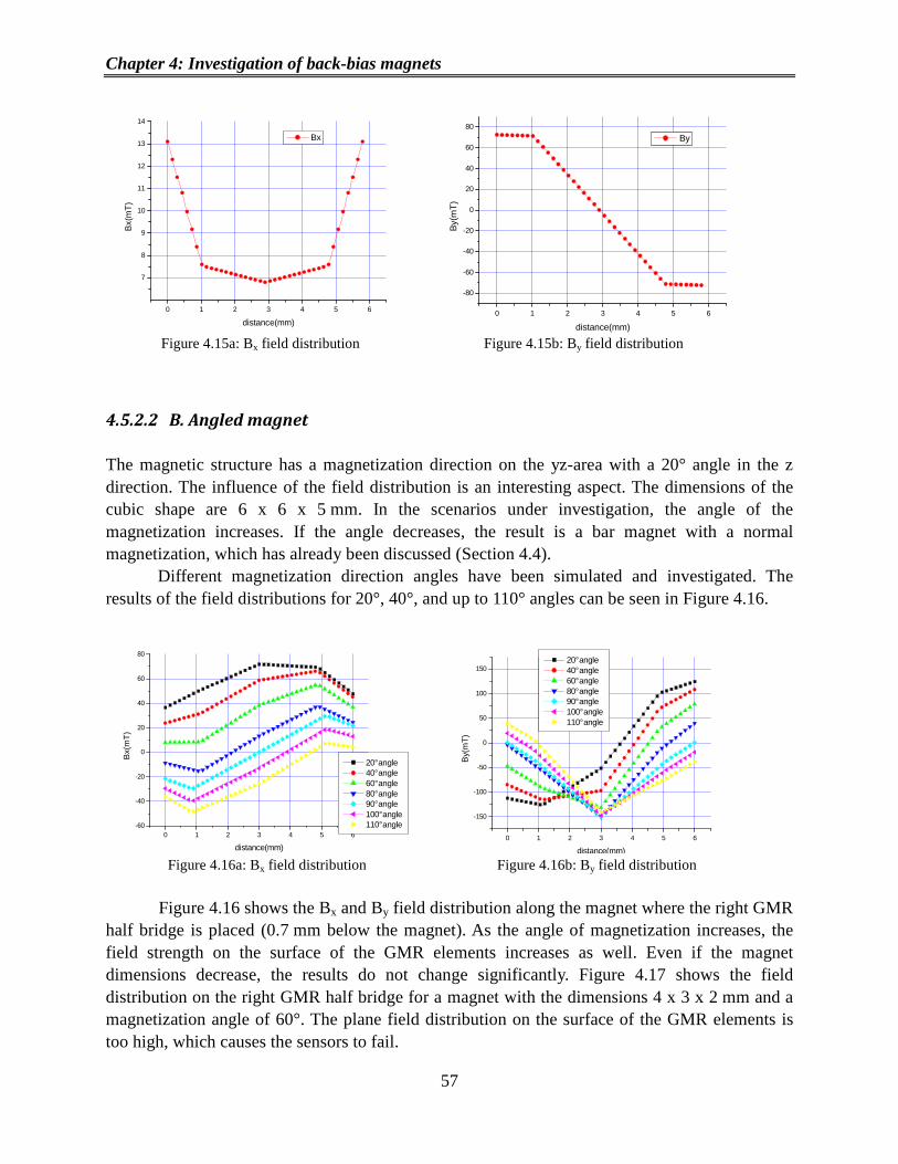
Chapter 4: Investigation of back-bias magnets
57
0 1 2 3 4 5 6
7
8
9
10
11
12
13
14B
x(m
T)
distance(mm)
Bx
0 1 2 3 4 5 6
-80
-60
-40
-20
0
20
40
60
80
By(
mT
)
distance(mm)
By
Figure 4.15a: Bx field distribution Figure 4.15b: By field distribution
4.5.2.2 B. Angled magnet
The magnetic structure has a magnetization direction on the yz-area with a 20° angle in the z direction. The influence of the field distribution is an interesting aspect. The dimensions of the cubic shape are 6 x 6 x 5 mm. In the scenarios under investigation, the angle of the magnetization increases. If the angle decreases, the result is a bar magnet with a normal magnetization, which has already been discussed (Section 4.4).
Different magnetization direction angles have been simulated and investigated. The results of the field distributions for 20°, 40°, and up to 110° angles can be seen in Figure 4.16.
0 1 2 3 4 5 6-60
-40
-20
0
20
40
60
80
Bx(
mT
)
distance(mm)
20° angle 40° angle 60° angle 80° angle 90° angle 100° angle 110° angle
0 1 2 3 4 5 6
-150
-100
-50
0
50
100
150
By(
mT
)
distance(mm)
20° angle 40° angle 60° angle 80° angle 90° angle 100° angle 110° angle
Figure 4.16a: Bx field distribution Figure 4.16b: By field distribution
Figure 4.16 shows the Bx and By field distribution along the magnet where the right GMR half bridge is placed (0.7 mm below the magnet). As the angle of magnetization increases, the field strength on the surface of the GMR elements increases as well. Even if the magnet dimensions decrease, the results do not change significantly. Figure 4.17 shows the field distribution on the right GMR half bridge for a magnet with the dimensions 4 x 3 x 2 mm and a magnetization angle of 60°. The plane field distribution on the surface of the GMR elements is too high, which causes the sensors to fail.

Chapter 4: Investigation of back-bias magnets
58
0.0 0.5 1.0 1.5 2.0 2.5 3.0-20
-10
0
10
20
Bx(
mT
)
distance(mm)
Bx
0.0 0.5 1.0 1.5 2.0 2.5 3.0
-35
-30
-25
-20
-15
By(
mT
)
distance(mm)
By
Figure 4.17a: Bx field distribution Figure 4. 17b: By field distribution
The angled magnetization magnet is a suitable solution only if the magnetic sensor is placed further away from the back bias magnet.
4.5.2.3 C. Cone magnet
A possible structure investigated is the cone geometry magnet (see Figure 4.13c).
Initially, the large base has a radius of 3 mm, and the radius of the small base is 1.5 mm. The height of the cone is 5 mm and magnetization has its direction on the normal axis (scenario 1). Two extra scenarios, one with smaller dimensions, namely scenario 2, with a radius of the large base of 2 mm and a radius of the small base of 1 mm, and another cone with a height of 7 mm (scenario 3) have been simulated. The Bx and By field distribution along the face of the magnet and at a distance of 0.7 mm below the magnet for the three simulated scenarios are shown in Figure 4.18.
-0.2 0.0 0.2 0.4 0.6 0.8 1.0 1.2 1.4 1.6 1.8
-170
-165
-160
-155
-150
-145
-140
-135
-130
-125
-120
-115
-110
-105
-100
-95
-90
Bx(
mT
)
distance(mm)
sc1 sc2 sc3
-0.2 0.0 0.2 0.4 0.6 0.8 1.0 1.2 1.4 1.6 1.8
-100
-50
0
50
100
By(
mT
)
distance(mm)
sc1 sc2 sc3
Figure 4.18a: Bx field distribution Figure 4.18b: By field distribution
Field distributions have been simulated on a path where the left half bridge GMR elements are being placed. More precisely, the GMR elements are situated at the center of the face of the magnet. The results reveal a huge Bx strength on the surface of the GMR elements, which reach saturation. These results show that the cone geometry is not suitable for the current application.

Chapter 4: Investigation of back-bias magnets
59
4.5.2.4 D. Two-tilted magnetic structure
Two bar magnets with a tilted magnetization direction in the xz area are placed next to
each other (see Figure 4.13d). Such structures imitate the U-shaped magnet distribution. At first, the magnetization of magnets forms a 20° angle in the normal direction (z-axis). The dimensions of both magnets are 3 x 6 x 5 mm on x-, y-, and z-axis. If the angle of the magnetization is reduced, the structure approximates the bar magnets (see chapter 4.4). If the magnetization angle is increased, the field intensity should be monitored. The results of the field distribution for the magnetization angles of 20°, 40°, and 60° are depicted in Figure 4.19.
0 1 2 3 4 5 6-20
-10
0
10
20
30
40
50
60
70
80
90
100
Bx(
mT
)
distance(mm)
20° tilt angles 40° tilt angles 60° tilt angles
0 1 2 3 4 5 6-100
-80
-60
-40
-20
0
20
40
60
80
100
By(
mT
)
distance(mm)
20° tilt angles 40° tilt angles 60° tilt angles
Figure 4.19a: Bx field distribution Figure 4. 19b: By field distribution
Figure 4.19 shows the Bx and By field distribution on a path along the magnet at a
distance of 0.7 mm below the face of the magnet. The field GMR elements sense a high plane field on the surface of the elements which reach saturation. Such a structure is not a suitable solution either.
4.5.2.5 E. Magnet with V-iron plate
An extra iron plate with a V-shaped geometry is placed beneath a bar magnet (see Figure
4.13e). Such a structure can assure that the field distribution decreases. Moreover, the field distribution on the GMR elements is more homogeneous when using this structure. A magnet with the dimensions 6 x 6 x 5 mm is attached to the V-shaped iron with a distance of 2 mm in the z-direction between the magnet and the wedge of the iron plate (see Figure 4.20a). The in-plane field distribution Bx can be seen in Figure 4.20b.

Chapter 4: Investigation of back-bias magnets
60
0 1 2 3 4 5 6
-14
-13
-12
-11
-10
-9
-8
-7
-6
Bx(
mT
)
distance(mm)
sc3
Figure 4.20a: Investigated structure Figure 4.20b: Bx field distribution
The field distribution on the surface of the GMR elements leads to saturation. Nevertheless, the magnetic field created can be optimized to meet the specifications of the applications.
4.5.3 Optimization process and analysis
The last structure, the bar magnet with a V-iron plate, was optimized to fulfill the magnetic field intensity specifications. Keeping the dimensions of the magnet as well as the magnetization and direction stable, the iron plate geometry and dimensions were changed in a way to meet the required flux density of Bx ~ 2 mT. The optimization procedure followed the loop shown in Figure 4.3. The calculated flux density Bx was on a node at the center of the surface of the GMR stripes. Whenever the simulated flux density was over 2 mT, the geometry of the iron plate has been increased in a specified step and the flux density was again recalculated. The optimized structure with the dimensions of the V-plate can be seen in Figure 4.21a. The magnet dimensions were 6 x 6 x 5 mm. The Bx magnetic field distribution along the edge of the magnet in the direction of the right half bridge GMR elements can also be seen in Figure 4.21b. The GMR elements are placed at the center of the face of the magnet in a distance of 0.7 mm below the face of the magnet.
0.5 mm
4 mm
3 mm 3 mm
3.25 mm
x
z
0.5 mm
0 1 2 3 4 5 6
-2
0
2
4
6
8
10
Bx(
mT
)
distance(mm)
B
Figure 4.21a: Optimized structure Figure 4. 21b: Bx field distribution

Chapter 4: Investigation of back-bias magnets
61
The field distribution on the surface of the GMR elements, as can be observed in Figure 4.21b, is less than 2 mT. The flux density at the center of the stripes is 1 mT.
4.5.4 Simulated rotational results
The performance of the magnetic structure can be estimated when performing static 3D simulations of a magnetic structure under open circuit conditions. In this case, the magnetic field on the surface of the GMR elements was calculated. For a proper estimation of the magnetic field distribution, it would be necessary to consider the magnetic circuit configuration in the simulation setup. For the optimized structure, a gear wheel with a pitch of 6 degrees and a tooth height of 3 mm was chosen. Figure 4.22a, shows the simulated 3D results of the magnetic circuit.
0 1 2 3 4 5 6-2.6
-2.4
-2.2
-2.0
-1.8
-1.6
-1.4
-1.2
-1.0
-0.8
-0.6
-0.4
Bx(
mT
)
angle(°)
Figure 4.22a: Simulated circuit model Figure 4.22b: Bx field distribution
Figure 4.22b shows the Bx field distribution on the surface of the left GMR element while
the gear wheel is rotating. The curve has a sinusoidal form and the field density for 0° is the same as the strength of 6° when the wheel is rotating. The air gap for these simulations was 4 mm, which was also the specification for the circuit performance. The GMR element does not reach saturation. Experimental results show that this proposed magnetic structure is able to operate properly up to an air gap of 4.5 mm.
4.6 Investigation of an iBB (integrated Back-Bias) magnetic structure Another magnetic structural design, suitable for automotive magnetic circuits, is illustrated in Figure 4.23. The magnetic sensor is inside the configuration. Figure 4.23 shows where the GMR elements are being placed. The position of the sensor is fixed. Additionally, this structure leads to a perfect positioning of the sensor in relation to the back bias magnet. As there is no possibility of slight variations in the position of the sensor regarding the magnet, offset problems are avoided.

Chapter 4: Investigation of back-bias magnets
62
Figure 4.23: New magnetic structure design
If the position of the magnet or of the sensing elements is asymmetric, offset problems occur. The results can clearly be seen in Figure 4.24. The sinusoidal magnetic field has an offset distribution from the starting point of the graph as indicated by the red arrow. Offset issues can create various problems for the calculation of the signal output, since the IC of the sensor might sense that the GMR elements are in a saturation mode and thus display a stable line as the output signal.
Figure 4.24: Offset calculation for a rotation of 1 pitch
The geometry structure in Figure 4.23 was investigated and a 3D FEM simulation was
performed to calculate the field distribution on the surface of the GMR elements. A ferrite magnet with a linear second quadrant demagnetization curve and a remanence of BR = 660 mT was used. The plane field distributions Bx and By along a path, where the left GMR element is located, can be seen in Figure 4.25. The GMR elements are at the center of the path. The field distributions of Figure 4.25a, and Figure 4.25b show that the field distribution is above the critical point and that the elements should be in a saturation mode. This can be seen more clearly
in Figure 4.25c, in which the plane distribution 22yxplane BBB += on the surface of the left
GMR is displayed. The flux density is over 15 mT. The GMR elements will definitely reach saturation.
Offset by misaligning btw. sensor and magnet

Chapter 4: Investigation of back-bias magnets
63
1.6 1.8 2.0 2.2 2.4 2.6 2.812
14
16
18
20
22
24
26
28
Bpl
ane(
mT
)
distance(mm) Figure 4.25c: Bplane on the surface of GMR
Experimental results have shown that for air gaps of approximately 1 mm, the sensor
delivers an output signal showing the movement of the gear wheel. This means that the GMR elements sense the changes of the flux density while the gear wheel is rotating, which is in complete contrast to the simulated results. This abnormality can be explained on the basis of the changes of the GMR’s sensitivity due to the influence of the y-direction of the field distribution on the surface of the GMR elements. This y-direction is in-plane but perpendicular to the easy axis of the free layer.
The ability of the GMR elements to detect the magnetic field is called sensitivity. In the graph of the output signal (Figure 1.4), the slope of the transfer curve gives the sensitivity of the GMR elements. To investigate the GMR sensitivity, the magnetic sensor was located in a Helmholtz coil experimental arrangement. The Helmholtz coil is a device producing a uniform magnetic field. It consists of two identical circular coils. Both coils have the same radius and electrical current. The tested device is placed between the two coils at the center along the common axis of the two coils to ensure that the magnetic field passing through has a uniform configuration. For coils with n turns and a current flowing through them, the magnetic flux density at the center is determined by equation 4.1. The sensor is placed between the two coils.
0 1 2 3 4 52
4
6
8
10
12
14
16
Bx(mT)
distance(mm)
0 1 2 3 4 5-150
-100
-50
0
50
100
150
By(mT)
distance(mm) Figure 4.25a: Bx field distribution along the
path Figure 4.25b: By field distribution along the
path
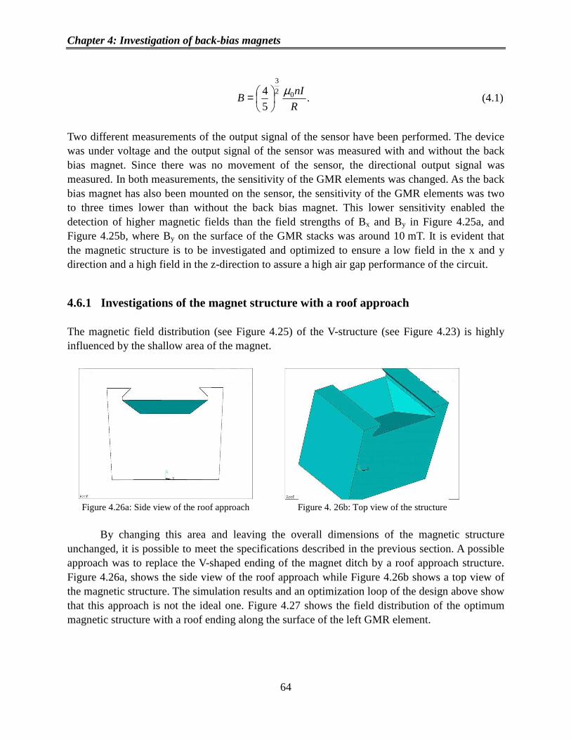
Chapter 4: Investigation of back-bias magnets
64
.5
4 02
3
R
nIB
µ
= (4.1)
Two different measurements of the output signal of the sensor have been performed. The device was under voltage and the output signal of the sensor was measured with and without the back bias magnet. Since there was no movement of the sensor, the directional output signal was measured. In both measurements, the sensitivity of the GMR elements was changed. As the back bias magnet has also been mounted on the sensor, the sensitivity of the GMR elements was two to three times lower than without the back bias magnet. This lower sensitivity enabled the detection of higher magnetic fields than the field strengths of Bx and By in Figure 4.25a, and Figure 4.25b, where By on the surface of the GMR stacks was around 10 mT. It is evident that the magnetic structure is to be investigated and optimized to ensure a low field in the x and y direction and a high field in the z-direction to assure a high air gap performance of the circuit.
4.6.1 Investigations of the magnet structure with a roof approach The magnetic field distribution (see Figure 4.25) of the V-structure (see Figure 4.23) is highly influenced by the shallow area of the magnet.
Figure 4.26a: Side view of the roof approach Figure 4. 26b: Top view of the structure
By changing this area and leaving the overall dimensions of the magnetic structure
unchanged, it is possible to meet the specifications described in the previous section. A possible approach was to replace the V-shaped ending of the magnet ditch by a roof approach structure. Figure 4.26a, shows the side view of the roof approach while Figure 4.26b shows a top view of the magnetic structure. The simulation results and an optimization loop of the design above show that this approach is not the ideal one. Figure 4.27 shows the field distribution of the optimum magnetic structure with a roof ending along the surface of the left GMR element.

Chapter 4: Investigation of back-bias magnets
65
1.6 1.8 2.0 2.2 2.4 2.6 2.8
-11.5
-11.0
-10.5
-10.0
-9.5
-9.0B
x(m
T)
distance(mm)
1.6 1.8 2.0 2.2 2.4 2.6 2.8
-8
-6
-4
-2
0
2
4
6
8
By(
mT
)
distance(mm) Figure 4.27a: Bx field distribution Figure 4.27b: By field distribution
By is approximately 7 mT. Bx has a value of -10 mT. In such a case, the sensitivity of the GMR elements increases, which leads to a decrease in the air gap performance of the magnetic sensor. The benefit of the air gap performance is minor in comparison to the first structure of Figure 4.23. More investigations of the ditch structure are needed to fulfill the specification of magnetic circuits with an air gap of at least 4 mm.
4.6.2 Pyramid structure approach – investigation and optimization
Replacing the roof geometry by a pyramid structure is another approach with promising results. A scheme of the magnetic structure is shown in Figure 4.28. A hollow pyramid structure substitutes the roof approach (see Figure 4.26b). The apex of the pyramid is inside the volume of the structure (see Figure 4.28a). The overall dimensions of the magnetic structure are the same as the dimensions of the magnet of Figure 4.23. The dimensions and the shape of the pyramid have been investigated. The height of the pyramid or the perpendicular distance from the base to the apex of the pyramid was the variable to be analyzed and optimized. The reference object function was the field distribution in the central point of the surface of the left GMR element. At that point, By had to be minimized, having been set, as a starting value, to be 20 mT. In order to apply the optimization loop method, the direct problem approximation was used. In this case, the finite element model is executed and solved while the suitable objective function is optimized. Starting from an initial geometrical dimension the minimization routine was carried out step by step to meet the objective function requirements. For a first z0 point the next point under investigation was:
zk+1=zk+λs (4.2) with λ a scalar number and s the search direction in the region under investigation. By giving a new z number, a new finite element model is created, re-meshed and solved to get the new objective function. At the end the resulting objective function there should be either the

Chapter 4: Investigation of back-bias magnets
66
minimum value under investigation or even a better solution in comparison with the initial objective function.
Figure 4.28a: Cross section of the view of the
pyramid Figure 4.28b: Top view of the pyramid structure
The resulting field distribution of the optimized structure is shown in Figure 4.29. The Bx and By field distribution have been calculated along the left GMR element and show a relatively small Bx of ~ 5 mT and a high By of 17 mT. This means that GMR sensitivity will be small and a high air gap performance can be achieved. Experimental results have shown that for certain gear wheel geometries the air gap performance of this structure can reach up to 4.5 mm. Figure 4.29c
shows the plane field distribution along the surface of the GMR element 22yxplane BBB += . The
maximum value of the plane field value is around 18 mT.
1.6 1.8 2.0 2.2 2.4 2.6 2.8
2.5
3.0
3.5
4.0
4.5
5.0
Bx(
mT
)
distance(mm) 1.6 1.8 2.0 2.2 2.4 2.6 2.8
-20
-15
-10
-5
0
5
10
15
20
By(
mT
)
distance(mm) Figure 4.29a: Bx field distribution Figure 4.29b: By field distribution

Chapter 4: Investigation of back-bias magnets
67
1.6 1.8 2.0 2.2 2.4 2.6 2.8
4
6
8
10
12
14
16
18
Bplane
(mT)
distance(mm) Figure 4.29c: Bplane field distribution
In Figure 4.28a, the two extra triangular parts on the front of the magnetic structure are
marked with the red circle. These are called the “ears” of the geometry. Their function is to hold the package of the GMR sensor tide but also to control the field distribution. In addition, it would be interesting to investigate the overall performance of the structure with and without the “ears” for construction reasons.
1.6 1.8 2.0 2.2 2.4 2.6 2.8
2.5
3.0
3.5
4.0
4.5
5.0
5.5
6.0
6.5
Bx(
mT
)
distance(mm)
Bx of No-Ears structure Bx of structure with Ears
1.6 1.8 2.0 2.2 2.4 2.6 2.8
-20
-15
-10
-5
0
5
10
15
20
By(
mT
)
distance(mm)
By of No-Ears structure By of structure with Ears
Figure 4.30a: Bx field comparison Figure 4.30b: By field comparison
Figure 4.30 shows the field distribution on the left GMR surface for the magnetic structure with and without the “ears.” The By distribution is almost the same. The Bx field distribution shows a shift of almost 2 mT. Comparing the plane field distribution on the surface of the GMR elements, it becomes evident that both structures reveal similar field values (see the B plane field distribution comparison on Figure 4.31).
The approach with no “ears” should also be a possible magnetic structure for the magnetic circuit application in question.

Chapter 4: Investigation of back-bias magnets
68
1.6 1.8 2.0 2.2 2.4 2.6 2.8
4
6
8
10
12
14
16
18
Bplane
(mT)
distance(mm)
Bx of No-Ears structure Bx of structure with Ears
Figure 4.31: B plane field comparison
Investigating the change in the magnetic flux density, while one of the dimensions of the
magnetic structure changes, is another interesting experiment. When decreasing the y-dimension of the geometry to 1.12 mm, the field increases. This is shown in Figure 4.32. The comparison of the B plane field distribution on the surface of the GMR elements for the geometries is demonstrated.
1.0 1.2 1.4 1.6 1.8 2.0 2.2 2.4 2.6 2.8
4
6
8
10
12
14
16
18
20
22
24
26
Bpl
ane(m
T)
distance(mm)
initial structure smaller structure
Figure 4.32: B plane field comparison of the two structures
In this case, the By field is too large and the GMR elements reach saturation. Not only the
height of the pyramid should be considered but the overall dimensions of the geometry. Finally, the influence of the flux density has been investigated when the magnetization direction slightly changes. Simulations were performed for a tilted magnetization of °± 5 on the yz and xz-planes. The comparative results of the Bx and By field distributions on the left GMR element and for the five cases, normal magnetization and tilted magnetization on the two planes, can be seen in Figure 4.33.
The results show that the Bx distribution and the normal and tilted magnetization on the zy-plane have similar values. The By distribution and the normal and tilted magnetization on the zx-plane likewise show similar values. Comparing the plane field -distributions on the surface of the GMR elements for the five magnetization directions reveals that the normal magnetization

Chapter 4: Investigation of back-bias magnets
69
direction has a similar distribution compared to the tilted magnetization directions on the zx-plane.
1.6 1.8 2.0 2.2 2.4 2.6 2.8
0.0
0.5
1.0
1.5
2.0
2.5
3.0
3.5
4.0
4.5
5.0
5.5
6.0
6.5
7.0
7.5
Bx(
mT
)
distance(mm)
B C D E F
1.6 1.8 2.0 2.2 2.4 2.6 2.8
-30
-25
-20
-15
-10
-5
0
5
10
15
20
25
30
By(
mT
)
distance(mm)
B C D E F
Figure 4.33a: Bx field comparison Figure 4. 33b: By field comparison
On the other hand, the tilted magnetizations direction on the ZY area has very high flux
density values and should thus be avoided (see the comparisons of Figure 4.34).
1.6 1.8 2.0 2.2 2.4 2.6 2.8
2
4
6
8
10
12
14
16
18
20
22
24
26
28
30
Bpl
ane(m
T)
distance(mm)
B C D E F
Figure 4.34: B plane field comparison
4.7 Investigation of the angle of magnetization on GMR stripes
The GMR elements, which are used in sensor technology, consist of a pinned layer with a magnetization direction that is perpendicular to the direction of the free axis of the free layer. Furthermore, the easy magnetization axis of the free layer is always placed perpendicular to the easy axis of the magnets. By calculating the field distribution on the surface of the GMR elements, it is possible to evaluate and measure the magnetization direction and to calculate the

Chapter 4: Investigation of back-bias magnets
70
change of the resistance of the GMR elements. The change of the angle of magnetization of the free layer can be seen in Figure 4.35.
Figure 4.35: Creation of an angle θ on the free layer of GMR element
The gray shading in Figure 4.35 indicates the separating spacer layer. The pinned layer has a fixed magnetization direction along the x-axis. The magnetization of the free layer fluctuates according to the plane field distribution on its surface. The relation of the resistance of the GMR element to the angle θ between the free and the pinned layer is calculated by means of the general GMR resistivity equation which was presented in the first chapter.
For a bar magnet with the dimensions x = 3 mm, y = 0.8 mm, and z = 0.4 mm, the magnetic sensor should have a distance of 0.35 mm. The magnet is ferrite with a remanence of Br
= 150 mT and a magnetization direction along the y-axis (see Figure 4.36).
x
y
z
1 mm 0.65 mm
0.4 mmz
Figure 4.36: Geometry of the application
The field distribution on the surface of the elements on the left half of the GMR bridge
can be seen in Figure 4. 37 where the in-plane Bx and normal to that, By field distribution (according to the coordinate system of Figure 4.36) on the left half bridge GMR element are presented. The By field distribution along the surface of the elements is distributed homogeneously.

Chapter 4: Investigation of back-bias magnets
71
Figure 4. 37a: Bx field distribution along the left
GMR1 Figure 4.37b: By field distribution along the left
GMR1
The angle θ between the pinned magnetization direction and the magnetization of the free layer of the GMR stack is given in the following equation:
.arctan
=
y
x
B
Bθ (4.3)
When substituting the Bx and By values from Figure 4. 37, the change of the angle θ according to equation 4.3, along the GMR surface can be displayed. The results can be seen in Figure 4.38.
Figure 4.38: Angle distribution on the surface of
GMR1
The fluctuation of the magnetization angle along the surface of the GMR elements is distributed uniformly, allowing the resistance of the elements to have a cosine response over the magnetization angle. An example of how this response is not achieved can be seen in Figure 4. 39. In this case, the magnetization of the bar magnet is in the normal direction. The dimensions of the magnet and its remanence are the same as before. The By field distribution in this case is
-0.8
-0.6
-0.4
-0.2
0
0.2
0.4
0.6
0.8
0
0.05
668
0.11
336
0.17
004
0.22
672
0.28
34
0.34
008
0.39
676
0.45
344
0.51
012
0.56
68
0.62
348
0.68
016
0.73
684
0.79
352
0.85
02
distance(mm)
Bx(
mT
)
Bx left GMR-1
-3
-2.5
-2
-1.5
-1
-0.5
0
0
0.05
668
0.11
336
0.17
004
0.22
672
0.28
34
0.34
008
0.39
676
0.45
344
0.51
012
0.56
68
0.62
348
0.68
016
0.73
684
0.79
352
0.85
02
distance(mm)
By(
mT
)
By left GMR-1
-25
-20
-15
-10
-5
0
5
10
15
20
25
0
0.05
668
0.11
336
0.17
004
0.22
672
0.28
34
0.34
008
0.39
676
0.45
344
0.51
012
0.56
68
0.62
348
0.68
016
0.73
684
0.79
352
0.85
02
distance(mm)
thet
a(°)
left GMR-1

Chapter 4: Investigation of back-bias magnets
72
not distributed uniformly along the surface of the GMR element (see Figure 4. 39), forcing the angle of magnetization to jump from a positive to a negative value. This can be seen in Figure 4.39b.
Figure 4. 39a: By field distribution on the surface
of GMR1
Figure 4. 39b: Angle distribution on the surface of GMR1
The angle over the distance of the GMR elements jumps to the center of the surface. This
jump can also be seen in the response to the GMR resistance, losing the cosine measuring signal and introducing an unstable output GMR signal. It was reported that such conditions can be found in high By external fields where moments of the GMR elements at the center and on the edges of the stripes have an anti-parallel response.
4.8 Conclusion
Back bias magnets used for automotive magnetic circuit applications were investigated [69] and [70]. Furthermore, the response and the field distribution were calculated. The flux density produced by a magnet is affected by numerous factors such as the dimensions of the magnet, its length, cross-sectional area, shape, and material. The magnetic field distribution, on the surface where the GMR elements are placed was calculated for different geometries and structures. Optimization procedures were used to fulfill the magnetic field distribution specifications on the GMR elements. Various simulated and optimized designs such as the structure in Figure 4.28 lead to an adequate working condition with an air gap performance in automotive applications over 4 mm.
The following chapter deals with the response and functionality of these magnetic structures in magnetic circuits applications. The working conditions will be calculated on the basis of simulations, and these conditions will be verified with the aid of experimental data.
-3
-2
-1
0
1
2
3
0
0.05
668
0.11
336
0.17
004
0.22
672
0.28
34
0.34
008
0.39
676
0.45
344
0.51
012
0.56
68
0.62
348
0.68
016
0.73
684
0.79
352
0.85
02
distance(mm)
By(
mT
)
By left GMR-1
-100
-80
-60
-40
-20
0
20
40
60
80
100
0
0.05
668
0.11
336
0.17
004
0.22
672
0.283
4
0.34
008
0.39
676
0.45
344
0.51
012
0.566
8
0.62
348
0.68
016
0.73
684
0.79
352
0.850
2
distance(mm)th
eta(
°)
angle for left GMR-1

Chapter 5: Investigation of Gear wheels
73
5 Investigation of Gear Wheels
The influence of gear wheels in automotive magnetic circuit applications is presented. A description of the problem, on how the geometry of gear wheels influences the detected field distribution on the surface of GMR elements is presented in section 5.1. In section 5.2 a typical magnetic circuit is presented and the field distribution is calculated at the surface of the GMR stack. Section 5.3 shows the effect of the gear wheel ratio, tooth distance to gap distance, and how it influences the field intensity calculated over the rotation of one pitch. Section 5.4 discusses the effect of tooth height on the magnetic field distribution, whereas section 5.5 examines how the magnetic field intensity fluctuates as the pitch dimensions are changed. Material issues of the gear wheel, more precisely the change in the permeability of the gear wheel, are examined in section 5.6. Finally, proposed new gear wheel geometries are investigated and the simulated field distribution is compared with the results of the initial gear wheel geometry.
5.1 Description of the problem
It is well known that field distribution at a point away from magnet is proportional to the area of the pole face of the magnet. Moreover, the field at a distance d from the pole face of the magnet is proportional to the inverse square of the distance given by equation 5.1
.1
2dB ∝ (5.1)
Apart from the dimensions and the shape of the magnet, the magnetic field created in automotive applications is also affected by the magnetic circuit itself as flux lines follow the paths with the lowest magnetic reluctance and always take the shortest path through any

Chapter 5: Investigation of Gear wheels
74
medium. Consequently, a complete investigation of the magnetic circuit and design is necessary to approximate the proper working conditions of the sensor. Magnetic circuits consist of a rotor part, which is the gear wheel, and the stator part, in this case the back bias magnet with a magnetic sensor. These variations of the magnetic field are detected by the magnetic sensor. The changed field distribution acts as the trigger signal and is transformed into an electrical signal, which is the output of the sensor. Due to the rotation the in-plane field distribution has a sinusoidal form. According to equation 5.1, the amplitude of this waveform decreases as the air gap increases. Both, the normal field distribution, which indicates the air gap performance, and the field distribution at the surface of the GMR elements, should be investigated in terms of the functionality of the GMR elements, and they should not reach the saturation mode. The influence of the gear wheel as well as the impact of different geometries and settings will be investigated and optimized in this chapter in order to show the functionality and to ensure the best possible performance of the sensor. Such investigations had been performed for 2D gear wheel structures [71].
5.2 Initial gear wheel simulations: Results and field distributions
In the initial magnetic circuit to be investigated, the back bias magnet is a bar magnet with the dimensions 10 x 10 x 4 mm as shown in Figure 5.1.
Figure 5.1: Initial magnetic circuit configuration
The magnetization direction is oriented in the normal direction. The magnetic sensor is
attached to the magnet and has two GMR elements. The gear wheel has a circular pitch with an angle of 6° and its teeth have a rectangular shape. The magnetic field distribution at the surface of each of the two GMR elements during the rotation of 1 pitch was simulated and evaluated. The air gap is the distance from the back of the sensor to the teeth of the wheel. This is shown in

Chapter 5: Investigation of Gear wheels
75
Figure 5.1. For comparison purposes, simulations for two air gaps with a distance of 1.5 mm (“air gap 1”) and 3 mm (“air gap 2”) will be carried out and discussed.
The normal (Bz field) distribution and the in-plane field distribution (Bx field) are shown in Figure 5. 2. The results shown are for a rotation of 6° (1 pitch) and an air gap of 1.5 mm. The field distributions were calculated at the center of the GMR elements.
0 1 2 3 4 5 6-108
-107
-106
-105
-104
-103
-102
-101
Bz(
mT
)
an g le (°)
0 1 2 3 4 5 6
-7
-6
-5
-4
-3
-2
-1
0
Bx(
mT
)
a n g le ( °) Figure 5. 2a: Normal field distribution Figure 5.2b: In-plane field distribution
The investigation are focused on the following aspects:
the effect of the tooth length on the field distribution while maintaining a constant pitch distance
the effect of the tooth height on the field distribution
the effect of changing different pitch distances
the effect on the field distribution while changing the gear wheel permeability
the effect of replacing the rectangular tooth by a smaller added rectangular tooth
For simplicity reasons, the back bias magnet always had the same dimensions and the same magnetization to show the impact of the gear wheel on the performance of the circuit. Useful conclusions should be drawn in order to choose the right gear wheel. Simulations were performed in three dimensions.
5.3 Effect of the tooth length on the field distribution
Firstly, the ratio of the thickness of the tooth and the space of the gap was investigated. Gear wheels for automotive applications usually have a ratio of 1:1, as can be seen in Figure 5.1, to assure a sinus field distribution along the in-plane axis.
As the position of the sensor is fixed, a maximum flux passes through the GMR elements, when the back-bias magnet is facing the tooth. However, if the magnet faces the gap of the
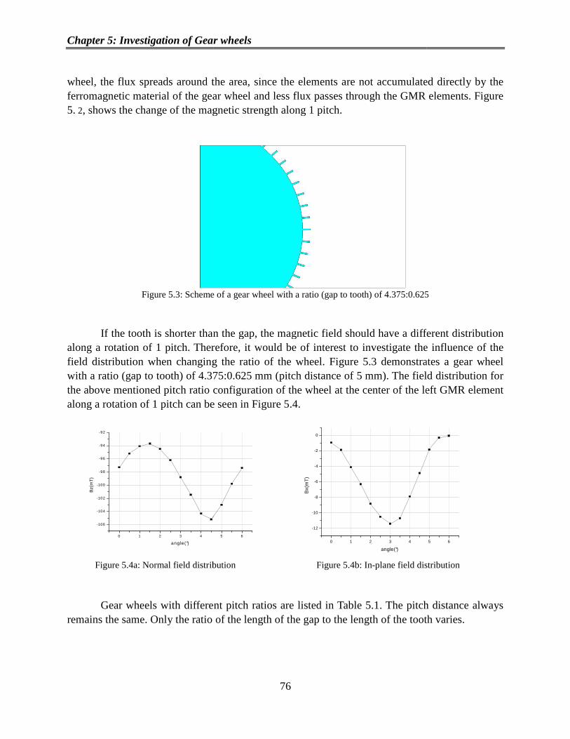
Chapter 5: Investigation of Gear wheels
wheel, the flux spreads around the areaferromagnetic material of the gear wheel and less 5. 2, shows the change of the magnetic strength along 1 pitch.
Figure 5.3: Scheme
If the tooth is shorter than the gapalong a rotation of 1 pitch. Therefore, field distribution when changing the ratio of the wheel. with a ratio (gap to tooth) of 4.375:0.625the above mentioned pitch ratio conalong a rotation of 1 pitch can be seen in
0 1 2 3 4
-106
-104
-102
-100
-98
-96
-94
-92
Bz(
mT
)
ang le(°)
Figure 5.4a: Normal field distribution Gear wheels with different
remains the same. Only the ratio of the length of the gap to the length of the to
of Gear wheels
76
around the area, since the elements are not accumulated direcferromagnetic material of the gear wheel and less flux passes through the GMR elements.
the magnetic strength along 1 pitch.
e of a gear wheel with a ratio (gap to tooth) of 4.375:0.625
than the gap, the magnetic field should have a different Therefore, it would be of interest to investigate the influence of
changing the ratio of the wheel. Figure 5.3 demonstrates a gear wheel tooth) of 4.375:0.625 mm (pitch distance of 5 mm). The field distribution for
pitch ratio configuration of the wheel at the center of the left GMR element along a rotation of 1 pitch can be seen in Figure 5.4.
5 6
0 1 2 3 4
-12
-10
-8
-6
-4
-2
0
Bx(
mT
)
angle(°)
Normal field distribution Figure 5.4b: In-plane field distribution
Gear wheels with different pitch ratios are listed in Table 5.1. The pitch distancethe same. Only the ratio of the length of the gap to the length of the tooth varies.
are not accumulated directly by the through the GMR elements. Figure
tooth) of 4.375:0.625
the magnetic field should have a different distribution the influence of the
demonstrates a gear wheel mm). The field distribution for
the center of the left GMR element
5 6
plane field distribution
itch distance always oth varies.

Chapter 5: Investigation of Gear wheels
77
Symbol RATIO LENGTH
(GAP: TOOTH) (MM) Gear1 1:4 Gear2 2.5:2.5 Gear3 3:2 Gear4 4:1 Gear5 4.5:0.5
Table 5.1: Investigated ratios
Figure 5.5 shows the comparison of the amplitudes for the different wheel ratios and for
the rotation of 1 pitch. The amplitudes of the field distribution refer to the left GMR stripe. Due to symmetry reasons, the results for the right GMR stripe are similar.
Figure 5.5a: Comparison of the amplitudes in the in-
plane direction Figure 5.5b: Comparison of the amplitudes in the normal
direction
When increasing the gap space, the in-plane field amplitude increases as well. Yet, the
comparison reveals that the optimum air gap performance is achieved with the geometry of Gear2 as in this configuration the amplitude of the normal field distribution is the highest. This geometry has the symmetrical configuration: the ratio is 1:1. Additionally, gear wheels with longer teeth in comparison to the length of gap show the worst performance in the circuit. As the field distribution is considerable high and can cause saturation in the GMR elements if using gear wheels with a ratio other than 1:1, the sensors should be placed at a distance underneath the back bias magnet to reduce the field intensity sensed by the elements.
5.4 Effect of the tooth height
The influence of the tooth height with regard to the field distribution, which is measured by the GMR elements, was likewise investigated. The initial gear wheel geometry had a tooth height of 3 mm, a typical height in automotive applications. Various tooth heights have been investigated with smaller and larger heights.
Amplitude comparison of in/plane field distribution
0
2
4
6
8
10
12
14
gear 1 gear2 gear3 gear4 gear5
ratio of gear wheels
Bx(
mT
)
AIRGAP1
AIRGAP2
Amplitude comparison of normal field distribution
0
1
2
3
4
5
6
7
gear 1 gear2 gear3 gear4 gear5
ratio of gear wheels
Bz(
mT
)
AIRGAP1
AIRGAP2

Chapter 5: Investigation of Gear wheels
78
With such an investigation, the optimal tooth height can be determined. Every change of the gear wheel changes the load line ratio B/H, which is evident of how the back-bias magnet will perform in the circuit. The B/H ratio is a parameter that is determined by the back bias magnet and the magnetic circuit characteristics in which the magnet operates.
Figure 5.6a: Comparison of the amplitudes in the normal
direction
Figure 5.6b: Comparison of the amplitudes in the in-plane direction
The amplitudes of the field distribution on the left GMR element were calculated for the
different tooth heights. The results for each of the two air gaps and for the normal and in-plane distribution are shown in Figure 5.6. Figure 5.6 also illustrates the comparison of the amplitudes for a rotation of 1 pitch along the left GMR element.
The comparison shows the increase of the field distributions in the normal and in-plane direction as the tooth height increases proportionally. Since magnetic fluxes have the tendency of taking the shortest way, increasing the height of the tooth leads to an accumulation of the fluxes on the surface of the tooth. Therefore, the field distribution increases in both directions.
5.5 Effect of different pitch distances
The influences on the field distribution when changing the pitch length of the gear wheel were investigated. Precautions were taken to keep the ratio of the thickness of the tooth and the space of the gap constantly at 1:1. Simulations for pitch lengths of 4, 5, and 6 mm have been performed. The initial gear wheels investigated (see Figure 5.1) had a pitch length of 5 mm with a gap and tooth length of 2.5 mm. When changing the pitch length, the angle of pitch also changes according to equation 5.2:
,θ⋅= Rl (5. 1)
where l is the length of the pitch arc, R is the radius, and θ is the angle of the pitch. For example, if the gear wheel has a pitch length of 6 mm and the same radius as the gear wheel in Figure 5.1, the pitch angle is 7.275°. Figure 5.7 shows the field distribution for the gear wheel with a pitch length of 6 mm. The normal and in-plane field distribution were simulated for the rotation of 1
Amplitude of normal field distribution Bz
0
1
2
3
4
5
6
7
2 3 4 5 6 7
tooth height (mm)
Bz(
mT
)
Airgap 1
Airgap 2
Amplitude of in-plane field distribution
0
0.5
1
1.5
2
2.5
3
3.5
2 3 4 5 6 7
tooth height (mm)
Bx(
mT
)
Airgap 1
Airgap 2

Chapter 5: Investigation of Gear wheels
79
pitch, and the field distributions were measured in a point at the center of the left GMR element. The air gap was 1.5 mm.
0 1 2 3 4 5 6 7 8
-108
-106
-104
-102
-100
-98
Bz(
mT
)
angle(°) -1 0 1 2 3 4 5 6 7 8
-10
-8
-6
-4
-2
0
2
Bx(
mT
)
angle(°) Figure 5.7a: Field distribution in the normal
direction Figure 5.7b: Field distribution in the in-plane
direction
Comparing the field distributions for a gear wheel with a pitch length of 6 mm with the
field distributions of the initial gear wheel (see Figure 5. 2), the magnetic field differs significantly. This can be observed clearly in Figure 5.8 in which the amplitudes of the in-plane and normal field distributions for each of the three gear geometries and for the two air gaps are illustrated, as they were measured at the left GMR element.
Figure 5.8a: Comparison of the amplitudes in the normal
direction Figure 5.8b: Comparison of the amplitudes in the in-plane
direction
When increasing the pitch distance, the field amplitude also increases both in-plane and in normal direction of the magnetic field. Taking this path, a greater air gap performance can be achieved without the GMR elements reaching saturation. Gear wheels with a large pitch distance would be the best solution in order to achieve a better magnetic circuit performance.
Amplitude of Normal field distribution Bz
0
1
2
3
4
5
6
7
8
9
10
4mm 5mm 6mm
pitch distance
Bz(
mT
)
Airgap 1
Airgap 2
Amplitude of in-plane field distribution
0
0.5
1
1.5
2
2.5
3
3.5
4
4.5
5
4mm 5mm 6mm
pitch distance
Bx(
mT
)
Airgap 1
Airgap 2

Chapter 5: Investigation of Gear wheels
80
5.6 Effect of changing the permeability of the soft magnetic gear wheel
With these simulations, the influence of the magnetic field, while changing the permeability of the gear wheel, have been investigated. Since the open magnetic circuit consists of the magnet, air with a relative permeability equal to 1, and the gear wheel, changing the wheel’s material properties can lead to a better performance of the magnetic circuit. Typical gear wheels used in automotive technology consist of 99.95 % pure iron annealed in hydrogen. Typical gear wheels have a relative permeability of 1500 to 4000.
In the simulations, the initial magnetic circuit, was used as can be seen in Figure 5.1. The
normal and in-plane field distribution have been calculated below the back bias magnet for four different relative permeability values of the gear wheel. The results were calculated at the center of the left GMR element. In each case, the air gap distance was the same. For the simulations material properties with relative permeability of 10, 100, 1000, and 10000 were chosen. Usually, the ferrite U60 has a µr of 10, while iron 99.8%, annealed has a µr around 100, and permalloy 45 has a relative permeability of around 1000.
The comparison of the Bx and Bz field distributions for a rotation of 1 pitch and a relative permeability of the gear wheel of 100 and 1000 can be seen in Figure 5.9. Figure 5.10 shows the comparison of the amplitudes of the normal and in-plane field distribution. The compared distributions show that neither in-plane fields nor normal fields significantly change with different relative permeabilities of the gear wheel.
Figure 5.10a: Comparison of the amplitudes in the
normal direction Figure 5.10b: Comparison of the amplitudes of in the in-
plane direction
Bz -Amplitude
0
0.2
0.4
0.6
0.8
1
1.2
mr=10 mr=100 mr=1000 mr=10000
relative magnetization
Bz(
mT)
Bx - Amplitude values
0
0.05
0.1
0.15
0.2
0.25
0.3
mr=10 mr=100 mr=1000 mr=10000
relative magnetization
Bx(
mT)
0 2 4 6-87
-86
-85
Bz(
mT
)
angle(°)
relative magnetization_100 relative magnetization_1000
0 2 4 6
-7.8
-7.6
-7.4
-7.2
Bx(
mT
)
angle(°)
relative magnetization_100 relative magnetization_1000
Figure 5.9a: Bz field distribution for two
different µr Figure 5.9b: Bx field distribution for two different
µr

Chapter 5: Investigation of Gear wheels
81
Magnetic flux lines always tend to follow the path with the greatest permeance. As a result, flux lines always take the shortest path through any permeable medium. Since the relative permeability of air is 1, the flux lines for greater wheel permeabilities are accumulated directly towards the gear wheel. That is why the amplitude of the field distribution in the in-plane and normal direction is quite stable. Therefore, the material properties of gear wheels do not play a crucial role regarding the performance of the magnetic sensors.
5.7 Effect of using an added rectangular tooth
Instead of a rectangular tooth other geometries, can be used as it can be seen in Figure 5.11. A shorter rectangular tooth (see Figure 5.11a) or a small triangular tooth (see Figure 5.11b) are added to the original tooth.
Figure 5.11a: Added rectangular tooth Figure 5.11b: Added triangular tooth
Gear wheels with an added rectangular or triangular tooth have the same configuration as
the wheel in Figure 5.1. They have the same pitch length, but only half of the tooth’s height has been replaced by the added structures, as shown in Figure 5.11.
Figure 5.12a: Comparison of the amplitudes in the
normal direction Figure 5.12b: Comparison of the amplitudes in the in-plane
direction
Amplitude of normal field distribution
0
1
2
3
4
5
6
7
8
9
initial gear added triangular added rectangular
gear wheel type
Bz(
mT
)
AIRGAP1
AIRGAP2
Amplitude of in-plane distribution
0
0.5
1
1.5
2
2.5
3
3.5
4
4.5
initial gear added triangular added rectangular
gear wheel type
Bx(
mT
)
AIRGAP1
AIRGAP2

Chapter 5: Investigation of Gear wheels
82
For the three different gear wheels discussed before, the field distributions below the magnet at the center of the left GMR element have been simulated. The comparison of the amplitudes for the normal and in-plane field distribution is shown in Figure 5.12.
The initial geometry shows a smaller normal distribution. Therefore, the air gap performance is not as great as with the other two gear wheel types. Additionally, the in-plane field distribution of the gear wheels with an added rectangular or triangular tooth is much higher than that of the initial gear wheel. The gear wheel geometry with an added triangular tooth does not drastically change the magnetic field distribution. Thus, the two new gear geometries can be used for magnetic circuits with a higher air gap performance. Especially when using an added rectangular tooth, a maximum performance of the magnetic circuit can be achieved. A 3D scheme of the new gear wheel geometry with a length of 0.5 mm is shown in Figure 5.13.
Figure 5.13: A 3D schematic view of the proposed gear wheel with added rectangular
Various gear wheels with different lengths of the added rectangular tooth have been
investigated and optimized. The comparison of the amplitudes of the normal and in-plane field distribution were measured at the center of the left GMR element. The various lengths of the added rectangular teeth can be seen in Figure 5.14.
Figure 5.14a: Comparison of the amplitudes in the
normal direction
Figure 5.14b: Comparison of the amplitudes of in the in-plane direction
When increasing the length of the rectangular tooth added, the in-plane and normal field
distribution decrease. Therefore, the field distribution of the initial gear wheel geometry is
Amplitude of normal distribution
0
0.5
1
1.5
2
2.5
3
3.5
4
4.5
5
added rect.0.625mm
added rect.0.5mm
added rect.0.75mm
added rect.1mm
added rect.1.5mm
length of added rectangular
Bz(
mT
)
AIRGAP1
AIRGAP2
Amplitude of in-plane distribution
0
1
2
3
4
5
6
added rect.0.625mm
added rect.0.5mm
added rect.0.75mm
added rect.1mm
added rect.1.5mm
length of added rectangular
Bx(
mT)
AIRGAP1
AIRGAP2

Chapter 5: Investigation of Gear wheels
83
reached. This can be seen in Figure 5.14. In a first approximation, the permeance of the air gap is given by the general equation (eq. 5.2):
,dxl
AP
g
gg ∫= (5.2)
where Ag is the air gap area and lg is the air gap length. Increasing the air gap area or reducing the air gap length will increase the ability of the magnetic fluxes to travel across the gap more easily. Therefore, the fringing flux decreases. However, that area has to be increased with care as the fringing flux is also related to these dimensions and increases with these dimensions.
Hence, the maximum field distribution is achieved for a length of 0.625 mm when keeping the air gap distance the same. Increasing this length leads to an increasing of the fringing flux. Further decreasing the length of the added rectangular decreases the permeability of the circuit as well, whence decreasing the field distribution. This is shown in equation 5.3.
As it can be seen in Figure 5.14, the field distributions in both the normal and in-plane direction of the gear wheel, which has an added rectangular tooth of 0.5 mm, are smaller than the field distribution for an added rectangular tooth with a length of 0.625 mm. A further interesting conclusion is that the length of the added rectangular tooth affects the field only in the case of small air gaps. With an air gap of 1.5 mm (Air gap 1), the field is influenced by the length. For bigger air gaps such as Air gap 2, 3 mm, the field strength is not affected as much. This can be explained again from equation 5.3, since air gap is inversely analog to the permeability of the circuit.
5.8 Conclusion
Different gear wheel geometries and structures have been investigated. Critical characteristics of the wheels, which have been examined and evaluated, were pitch dimensions, the tooth height, changes in the ratio of the teeth, different relative permeabilities of the ferromagnetic materials for gear wheels, and changes in the geometry due to added structures to the teeth [72]. For this reason, 3D models have been created and simulated with the field distributions at the surface of the GMR elements. With this method it is possible to get fast and efficient results in comparison with experiments in a costless way.
The results have shown that it is possible to design and optimize gear wheels used in magnetic circuits for automotive applications. Increasing the tooth height and/or the pitch distance, the field amplitude is increased both in normal and in-plane direction of the magnetic field. In such a case, the overall characteristics of the GMR magnetic circuit can be improved and a greater air gap performance can be achieved.
Moreover, by increasing the gap space and decreasing the tooth length, the in-plane field intensity increases and the normal field decrease. Additionally, when replacing the tooth by a

Chapter 5: Investigation of Gear wheels
84
smaller added rectangular tooth, it is possible to fulfill the investigated specifications. However, a drawback in the last case is that the manufacturing of this geometry is quite expensive in comparison to the other alternatives.

Chapter 6: Rotated magnetic circuit: Model development and verification
85
6 Rotated magnetic circuit: Model development and verification
This chapter presents the 3D model of the GMR-sensor magnetic circuit with gear wheel. Simulation results are compared with experiments and the results are detailed here. This chapter begins with the section 6.1, where the model description and its application are presented. Section 6.2 describes the methodology used for model creation. Following this in the next section, a specific magnetic circuit application with an angled back-bias magnet is simulated to calculate the field distribution on the GMR element surface. In particular two approaches of a magnetic circuit are examined. In the first approach, the model predicts the failure of this magnetic circuit configuration whereas in the second approach, the model validates the functionality of the application. The second circuit configuration is examined also with experiments, presented in Section 6.4. Section 6.5 shows the comparison between the simulated and experimental results. Simulations show a close agreement with the experiment thereby validating the proposed model.
6.1 Description of the problem
In previous chapters, the use of modeling and simulation in determining the proper structures of back-bias magnets and or gear wheel for use in the automotive applications was discussed intensively. These simulations could give indications of the magnetic field that GMR elements are sensing. However, this methodology does not ensure that the chosen magnetic circuit works perfectly within the sensor specifications. Due to high GMR sensitivity, it is important to know the field intensity the elements are sensing during the operation cycle of the magnetic circuit. If the GMR elements are working in the linear operating window, then the magnetic sensor is being properly operated, otherwise the GMR elements are in saturation mode and the sensor does not give any output signals. Therefore, it is very important to ensure that GMR sensors always stay in their linear operating range.

Chapter 6: Rotated magnetic circuit: Model development and verification
86
The method mostly used to investigate the functionality of the sensors is by experimental setup. Experimental data such as the output signal of the sensor could indicate the suitability of the magnetic circuit. The drawbacks of experiments are that they are costly and whenever different circuits’ characteristics are going to be investigated, changes also have to be made to the setup. Hence, experimental procedures are also time-consuming. The magnetic circuit could be simulated and investigated with the help of a finite element method (FEM) to overcome the previously mentioned problems. With the use of FEM, it is possible to calculate the field distribution in all three directions and find the field intensity at the surface of GMR elements for a rotation of the wheel with respect to the sensor location. Moreover, it is easy to change and investigate different characteristics of the magnetic circuit such as changes of gear wheel geometries, different air gaps or different back-bias magnetic structures and materials. Such changes can be achieved easier and much faster than in the case of an experimental procedure.
In the following chapter, the methodology to simulate a magnetic circuit with a GMR sensor is demonstrated and the investigation of the magnetic field at the surface of the GMR elements is presented. Finally, a comparison between simulated and experimental data will show a small deviation proving the adequacy of the simulating method.
6.2 Setting the 3D model
The magnetic circuit under investigation is depicted in Figure 6.1. The gear wheel consists of 44 teeth with a circular pitch of 8.18° degree angle. Each tooth has a height of 3 mm and the gear wheel has a depth (y-axis dimension) of 10 mm.
Figure 6.1: Magnetic circuit under investigation
The back-bias magnet consists of two separated magnets joined together each of which
has a tilted magnetization direction on the xz plane of 20°, measured from the z axis as shown in
Figure 6.1. The dimensions of the magnet are 10x10x4 mm. The magnet is a ferrite with a

Chapter 6: Rotated magnetic circuit: Model development and verification
87
remanence of Br=287 mT. The distance from the end of the sensor to the top of the tooth forms the air gap of the circuit. The field distribution along the surface (xy-plane) of the GMR elements was investigated. Additionally, the field distribution in the normal direction should be also calculated in order to determine the sensor response due to the changes of the air gap. Considering this explanation, it can be seen that the magnetic circuit should be investigated in 3D so that the simulated results can be compared to the experimental data.
For the creation of the model, the bottom-up approach is used [73]. This method offers the benefit of firstly, creating the primitives of the model and secondly, of forming the geometry, dividing it to elements to create the mesh and setting the DoFs. The advantage is that crucial parameters of the model under investigation are discretized and can easily be changed to repeatable executable simulations leading easily to new results for every change. The modeling procedure was that firstly, the geometrical model of the gear wheel and back-bias magnet was created in 2D and meshed. Then it was extracted in 3D using a bilinear 8-node element. Finally, the simulated model was executed and results were stored and investigated. The model was solved using the scalar potential approach. The model simulated consists of the gear wheel and the back-bias magnet. The magnetic sensor was omitted since it doesn’t influence the field distribution. The model was enclosed with air. Precautions have to be made for the air surrounding the magnetic structure. Dimensions should be 5 times the respective dimensions of the magnet so that results are converged without calculation errors. Due to lack of symmetry, the whole structure was simulated, including the gear wheel with the 44 teeth, the magnet and the surrounding air. Thereby, more precise results, close to real life measurements can be achieved.
On the other hand, simulating a part of the model using ANSYS, for example, the ¼ of the wheel, with the magnet and the corresponding air enclosure gives only reasonable results, for small air gaps distances, since the relative permeability of the iron gear wheel is too high compared with the relative permeability of the magnet and the air. Another issue on simulating a part of the model is to ensure the symmetry of the problem, since only a part of the design is modeled. This can be solved by setting the lateral flank faces of the model, under Dirichlet boundary conditions (Bnormal=0). In this case both sides’ nodes are coupled with the same degrees of freedom therefore, they are under the same conditions, the same field distribution. Additional care had to be taken for the overhanging nodes due to the rotation of the model. Overhanging nodes are the nodes of the interface surface of the rotated part of the model that, due to the movement procedure of that part, are no longer directly connected to the rest of the model. The overhanging nodes should always be modeled in a way to allow the edges (the nodes being there) of the two moved entities of the model to be aligned, securing the connectivity and continuity of the model.
To avoid this improper sequence and get reliable results the full model is simulated. Figure 6.2a, depicts the simulated model. Using FE modeling, the geometry is divided into a grid of smaller geometries. This implies that a part of the simulated model cannot be moved easily compared to the rest of the model - in this case, the gear wheel is to rotate about the sensor. There are several techniques which can be used to solve such a problem. A way to solve and imitate the rotation of the gear wheel is to create the model as it is depicted in Figure 6.2a.

Chapter 6: Rotated magnetic circuit: Model development and verification
88
Figure 6.2a: Simulated model Figure 6.2b: Connected FEM model
For each position of the magnet, the model is solved and the calculated field distributions
are stored. Next, the magnet is moved to a new position in front of the gear wheel and the model is solved again. This sequence will be continued for a pitch distance. Such a method denotes that each time the magnet is moved to a new position; the model has to be created from the beginning, meshed and solved. This method is time consuming and it enhances calculation errors, since the movement of the magnet changes the meshing surrounding the magnet. Another technique can be by using overlapping elements [74]. The model of Figure 6.2a, is divided in two parts and each of the parts is meshed separately. The two meshed parts are overlapped to form the simulated magnetic circuit model in an arbitrary manner.
A proper mechanism to model such a problem is by connecting the interface nodes. The model of Figure 6.2a, is divided in two parts. The first part, the inner part of the model consists of the gear wheel and the half air gap distance with the corresponding enclosure air. The remainder of the model, including the magnet with the surrounding air forms the outer part. Both parts have a common interface surface at the half of the air gap distance and are meshed separately from each other. To ensure the continuity of the model, the two separated parts must have their nodes connected at the interface surface. Figure 6.2b demonstrates the two different meshed parts and the connection of their interface nodes at the common shared surface. This is indicated with the red colored interface. The interfaced nodes from both sides are connected to each other using constraint equations [75].
Using the constraint equations technique, for the model under investigation (Figure 6.2b), the potential at a node belonging to the inner part must be equal to the opposite node potential, belonging to the outer part, as it is indicated in Equation 6.1.
!"#$%,'""%( !"#$%,#)*%(. (6.1)
Using the constraint equation method, it is possible to separately mesh and then connect
the two parts. Since the nodes on the interface surface are always joined to each other, it is

Chapter 6: Rotated magnetic circuit: Model development and verification
89
possible to rotate the inner part around the outer part. Every time a part moves towards the other part of the model, the interface nodes of the moving part of the model are always connected with the interface nodes of the other part of the model, securing the connectivity and continuity of the simulated model. In this way, always keeping the meshing of the model unaltered, it is possible to get the rotation movement of the wheel towards sensor and magnet with a do-loop. At the lateral outer part of the simulated model, infinite elements were performed to model the far-field decay of the field. Finally, the GMR sensor which will be investigated consists of a Wheatstone bridge GMR configuration, which measures the speed signal and a separated GMR element, located at the center of the chip responsible for the directional speed signal measurements. While the gear wheel is rotated for a distance of one pitch, the field distribution along the x-axis changes creates a sinusoidal field. This field distribution as well as the normal in-plane field distribution (y-axis) will be investigated and compared with experimental results.
6.3 Simulation results
6.3.1 Setting the magnet attached to the sensor
A first important issue in investigating the magnetic circuit of Figure 6.1 is to find the magnetic circuit configuration that provides the correct functionality of the GMR sensor. The GMR elements have a high sensitivity, and can therefore be driven at saturation. However, this can only occur if the external magnetic intensity is larger than a crucial value (depending on the GMR material properties). To prevent this malfunction of the sensor due to GMR’s saturation, it is very important to set the correct placement of the sensor between the gear wheel and the back-bias magnet.
Figure 6.3a: Bx field distribution on the left GMR Figure 6.3b: Bx field distribution on the center GMR
Bx field on the left GMR
-14
-12
-10
-8
-6
-4
-2
00 0.5 1 1.5 2 2.5 3 3.5 4 4.5 5 5.5 6 6.5 7 7.5 8 8.18
angle(°)
Bx(
mT
)
Bx field on the center GMR
-2
-1.5
-1
-0.5
0
0.5
1
1.5
2
0 0.5 1 1.5 2 2.5 3 3.5 4 4.5 5 5.5 6 6.5 7 7.5 8 8.18
angle(°)
Bx(
mT
)

Chapter 6: Rotated magnetic circuit: Model development and verification
Initially, the sensor was attached to the backgeneral, since it is easy to manufacture the package containing the backsensor, and therefore cheaper. Simulations for this configuration with an airgap of 2carried out. In Figure 6.3, the graphs show Bleft and center GMR stack. The field distributions were calculated for a rotation of 1 pitch on the surface of the GMR elements. The Bin Figure 6.3a, is approximately saturation. In this case, GMR elements are forced to work outside their working window range and cause a sensor malfunction. Similar conclusions, comparable with the above simulations were also derived by the experimental procedure. Performing measurements with attached to the back-side of the magnet, the calculated output signals are demonstr6.4. The blue, almost straight line indicates the speed output signal, as it is measured from the Wheatstone bridge GMR configuration. This signal is the subtractleft and the right half-bridge configuration signals.
Figure 6.
If the sensor works in GMR working linear range then it would have been expected that
the speed signal output had a sinusoidal shape. For instancthe tooth and the right half-bridge was facing the gap of the gear, then the difference in the measured field intensity would also have been shown in the output signal of the sensor. However, in this case, the straight line reveals that there is no change in the measured field by the tWheatstone half-bridges. This impliesthe GMR elements always sense the same field leading to miscalculations of the field distribution. Above simulations and experimental results is driving the GMR elements into saturation. A new configuration of the magnetic circuit has to be investigated to provide working conditions of the sensodistance. Therefore, the sensor should be kept at a distance from the back side of the magnet to correctly perform and measure the changes of the external magnetic field.
Rotated magnetic circuit: Model development and verification
90
the sensor was attached to the back side of the magnet. This case igeneral, since it is easy to manufacture the package containing the back-bias magnet and the
therefore cheaper. Simulations for this configuration with an airgap of 2the graphs show Bx, at a point in the center of the GMR elements for the
left and center GMR stack. The field distributions were calculated for a rotation of 1 pitch on the The Bx field distribution on the left GMR element as
approximately -10 mT which is big enough to drive GMR elements In this case, GMR elements are forced to work outside their working window range
milar conclusions, comparable with the above simulations were also derived by the
experimental procedure. Performing measurements with air gap of 2 mm and having the sensor side of the magnet, the calculated output signals are demonstr
. The blue, almost straight line indicates the speed output signal, as it is measured from the Wheatstone bridge GMR configuration. This signal is the subtracted signal calculated from the
bridge configuration signals.
Figure 6.4: Experimental sensor output results
in GMR working linear range then it would have been expected that a sinusoidal shape. For instance, when the left half-bridge was facing
bridge was facing the gap of the gear, then the difference in the would also have been shown in the output signal of the sensor. However,
ht line reveals that there is no change in the measured field by the timplies that for every placement of the sensor towards gear wheel,
the GMR elements always sense the same field leading to miscalculations of the field
Above simulations and experimental results show that the magnet is too strong to saturation. A new configuration of the magnetic circuit has to
working conditions of the sensor as well as a reasonable Therefore, the sensor should be kept at a distance from the back side of the magnet to
correctly perform and measure the changes of the external magnetic field.
This case is preferable in bias magnet and the
therefore cheaper. Simulations for this configuration with an airgap of 2 mm were of the GMR elements for the
left and center GMR stack. The field distributions were calculated for a rotation of 1 pitch on the field distribution on the left GMR element as can be seen
mT which is big enough to drive GMR elements into a In this case, GMR elements are forced to work outside their working window range
milar conclusions, comparable with the above simulations were also derived by the mm and having the sensor
side of the magnet, the calculated output signals are demonstrated in Figure . The blue, almost straight line indicates the speed output signal, as it is measured from the
signal calculated from the
in GMR working linear range then it would have been expected that bridge was facing
bridge was facing the gap of the gear, then the difference in the would also have been shown in the output signal of the sensor. However,
ht line reveals that there is no change in the measured field by the two placement of the sensor towards gear wheel,
the GMR elements always sense the same field leading to miscalculations of the field
magnet is too strong therefore to saturation. A new configuration of the magnetic circuit has to
r as well as a reasonable air gap Therefore, the sensor should be kept at a distance from the back side of the magnet to

Chapter 6: Rotated magnetic circuit: Model development and verification
91
6.3.2 Setting a gap between magnet and magnetic sensor
In the new circuit configuration, a gap of 2 mm has been kept between the back side of the magnet and the sensor package. The scheme of the new circuit setup is depicted in Figure 6.5. The magnetization direction of the free layer of GMR elements follows the external field distribution. In the design shown in Figure 6.5, the GMR stripes are situated along y-axis with a length of approximately 1 mm. In Chapter 3 (Section 3.12), the influence of the plane field distribution along the GMR surface and how the change of the plane field affects the magnetization direction of the free layer and in general, the resistivity of the GMR element has been described. Hence, to investigate the influence of the magnetic field to the GMR stack, it is important to simulate the plane field distribution on the surface of the stack, meaning the Bx and By field as it is indicated in Figure 6.5.
Figure 6.5: The new circuit geometry under investigation
For investigations of the plane magnetic field at the length of GMR stripe, the Bx and By
distributions were calculated at points which were equidistantly spaced. The bottom spot of the surface of GMR stripe is selected as the starting point for calculations (e.g. in Figure 4.1, the path where the points are lying at the surface is marked with red color) and it is denoted as the 0 point. The next point is spaced by 0.05 mm. These equally spaced deviations of the path are continued until the last point on the top side of the stripe which lies out of the paper in a direction perpendicular to it, along the y-axis.
Figure 6.6a: Bx distribution on a GMR on the left half-bridge Figure. 6.6b: By distribution on a GMR on the left half-bridge
-3.5
-3
-2.5
-2
-1.5
-1
-0.5
0
0.5
1
0 11.
5 22.
5 33.
5 44.
5 55.
5 66.
5 77.
5 8
8.18
18
angle(°)
Bx(
mT
)
Bx @ 0mm
Bx @ 0.05mm
Bx@ 0.1mm
Bx@ 0.15mm
Bx@ 0.2mm
Bx@ 0.25mm
Bx@ 0.3mm
Bx@ 0.55mm
Bx@ 0.6mm
Bx@ 0.65mm
Bx@ 0.7mm
Bx@ 0.75mm
Bx@ 0.8mm
Bx@ 0.85mm
Bx@ 0.9mm
Bx@ 0.95mm
Bx@ 1mm-2
-1.5
-1
-0.5
0
0.5
1
1.5
2
0 1 1.5 2 2.5 3 3.5 4 4.5 5 5.5 6 6.5 7 7.5 8 8.182
angle(°)
By(
mT
)
By@ 0mm
By@ 0.05mm
By@ 0.1mm
By@ 0.15mm
By@ 0.2mm
By@ 0.25mm
By@ 0.3mm
By@ 0.35mm
By@ 0.4mm
By@ 0.45mm
By@ 0.5mm
By@ 0.55mm
By@ 0.6mm
By@ 0.65mm
By@ 0.7mm
By@ 0.75mm
By@ 0.8mm
By@ 0.85mm
By@ 0.9mm
By@ 0.95mm
By@ 1mm

Chapter 6: Rotated magnetic circuit: Model development and verification
92
Figure 6.6c: Bx distribution on a center GMR element Figure 6.6d: By distribution a center GMR element
With this approach, we get a pattern of the plane field distribution along the surface of the
GMR elements. The Bx and By field distributions, of the equidistant with 0.5 mm spaced points, and for two GMR elements, one of which is located on the left half-bridge (Figure 6.6a-b) and another on the center of the sensor (Figure 6.6c-d) are demonstrated in Figure 6.6. Simulations were performed for a rotation of 1 pitch of the wheel along the back-bias magnet. Due to symmetry reasons, the plane field distribution of a GMR located in the right half-bridge would have the same By field distribution along GMR surface and reversed but same in magnitude, Bx field.
The Bx fields along the GMR stripes always have the same response for a rotation of 1 pitch. On the other hand the By field is shifted each time we move from the bottom side of the stripe towards the upper side. The By fields are homogeneously distributed along the stripes. At the center of the stripe, By distribution is approximately zero, and moving further up or down, the field has the same magnitude but reversed polarity. This is due to the symmetric external magnetic field created by the back-bias magnet.
6.4 Experimental results
For the configuration shown in Figure 6.6, experiments were performed and compared with the simulated data. Since the method of constraint equations was used to rotate the simulation model, it was possible to imitate the real magnetic circuit performance. But in reality, with this simulated method, a sequence of static simulations for every corresponding magnet position over the rotated angle was performed, having as a big advantage the meshing of the model which does not change during the simulations. Therefore, this approach gives faster and more accurate results.
So, to perform the experiments in the test bench and to compare the experimental with the simulations results, minimum wheel speed was chosen, in our case this was 1.5 rpm.
-2
-1.5
-1
-0.5
0
0.5
1
1.5
2
0 1
1.5 2
2.5 3
3.5 4
4.5 5
5.5 6
6.5 7
7.5 8
8.18
angle(°)
Bx(
mT)
Bx@ 0mm
Bx@ 0.05mm
Bx@ 0.1mm
Bx@ 0.15mm
Bx@ 0.2mm
Bx@ 0.25mm
Bx@ 0.3mm
Bx@ 0.35mm
Bx@ 0.4mm
Bx@ 0.45mm
Bx@ 0.5mm
Bx@ 0.55mm
Bx@ 0.6mm
Bx@ 0.65mm
Bx@ 0.7mm
Bx@ 0.75mm
Bx@ 0.8mm
Bx@ 0.85mm
Bx@ 0.9mm
Bx@ 0.95mm
Bx@ 1mm -2
-1.5
-1
-0.5
0
0.5
1
1.5
2
0 1 1.5 2 2.
5 3 3.5 4 4.
5 5 5.5 6 6.
5 7 7.5 8
8.18
18
angle(°)
By(
mT
)
By@ 0mm
By@ 0.05mm
By@ 0.1mm
By@ 0.15mm
By@ 0.2mm
By@ 0.25mm
By@ 0.3mm
By@ 0.35mm
By@ 0.4mm
By@ 0.45mm
By@ 0.5mm
By@ 0.55mm
By@ 0.6mm
By@ 0.65mm
By@ 0.7mm
By@ 0.75mm
By@ 0.8mm
By@ 0.85mm
By@ 0.9mm
By@ 0.95mm
By@ 1mm

Chapter 6: Rotated magnetic circuit: Model development and verification
93
Figure 6.7: Experimental output signals
As the gear wheel rotates, the magnetic sensor provides speed; this output comes from
the GMR elements situated in a Wheatstone bridge configuration which measures the speed of rotation of the wheel and the directional signal, which is the output of the GMR element situated at the center of the sensor. A drawback of the experimental procedure is that there is no possibility to derive the Bx and By distribution along the GMR stripes directly, but only the plane field distribution at the surface of the GMR elements while the gear wheel is rotated towards the magnetic sensor because the input signal to the sensor, the external magnetic field has a ratio 1:1 with the sensor’s output signal.
Figure 6.7 demonstrates the output sensor signals. The red curve indicates the measured directional signal, while the blue curve shows the speed signal. The x-axis of Figure 6.7 shows the angle of rotation of the gear wheel. The y-axis shows the output results in LSB (least significant bit). LSB gives the resolution of the measurement, determining the resolution of the ADC converter of the sensor. LSB values can be transformed to magnetic flux density using the following equation (Equation 6.2):
),(_
mTS
valueLSBB = (6.2)
where S is the sensitivity of the GMR elements. In this case the sensitivity was measured and found to be S=154.67 (LSB/mT).
6.5 Verification of simulation results with experimental results. Setting the field distribution along the GMR elements
As indicated in Figure 6.6, the By distributions are altered along the GMR elements, as Bx
keeps a constant value. The plane field (Bplane2=Bx
2+By2) on the surface of the stripes changes
due to the movement of the gear wheel. The average field that the elements are sensing has to be calculated and this field is to be compared with the experimental results of Figure 6.7.
-300
-200
-100
0
100
200
300
0.00
0.70
1.39
2.09
2.78
3.48
4.17
4.87
5.57
6.26
6.96
7.65
8.35
9.04
9.74
10.4
411
.13
11.8
312
.52
13.2
2
LSB
phi [°]
SPEED ADC
DIR ADC

Chapter 6: Rotated magnetic circuit: Model development and verification
94
The characteristic curve of the GMR elements which shows the magneto-resistive response of a spin valve, while the external magnetic field is varied (Figure 1.4) shows the linear working window of the GMRs as well as the 2 regions which correspond to GMR saturation mode . This curve is the result of experiments setting the GMR element on different external magnetic field values and measuring the output change of the resistivity. By fitting those experimental data it is possible to associate the Bx and By field distribution on the GMR surface with the resistance of the GMRs using the following equation (Eq. 6.3):
( )( )
,
1
1 6521
0,
43
−+
+
+−+=
+
y
BPP
B
yBB BPP
e
BPPGMRRR
y
xyx (6.3)
where, P1 to P6 are the fitting parameters. R0 is the initial resistance of the stack, without the presence of an external magnetic field, equal to 10 kΩ. GMR is a coefficient equal to 0.1. By substituting in the above equations the Bx and By data along the surface of the GMR elements results in the change of the resistance of the elements along their distance. Knowing the current density Ibias passing by the GMR elements by performing the Ohm law:
V=Ibias*R (6.4) we can derive the output response of the sensor.
The output signals are demonstrated in Figure 6.8. Figure 6.8a, shows all the created output signals along the surface of the elements. In the upper graph, the direction of the curves coming from the simulation results along the surface of the GMR stripe is depicted. In the lower graph we get the same results for the speed output signals. In both graphs the distribution with the red line indicates the experimental outputs. Blue lines are showing the respond of the plane magnetic field distribution for each simulated point across the GMR surface (Figure 6.6). Figure 6.8b demonstrates the results of the averaging theoretical signals in comparison with the experimental ones.

Chapter 6: Rotated magnetic circuit: Model development and verification
95
Figure 6.8a: Output signals for each position on the surface of the GMR elements
Figure 6.8b: The average output signals
This correlation between the simulation and experimental results is more clearly
explained if, with the help of Equation 6.3, we transform the signals to plane field distribution as it can be seen in Figure 6.9.
Figure 6.9a: Comparison of directional signal Figure 6.9b: Comparison of speed signal
The measured field curves are indicated by a blue line whereas the distributions calculated from the simulation model are indicated by the red line. Results are shown for a rotation of 1 pitch. Figure 6.9a shows the comparison between the experimental measured directional signal and the calculated signal. The deviation between those two curves has a mean value of 9%. Figure 6.9b compares the speed signal coming from measurements and simulations. In this case the mean deviation is small at approximately 3%.
Although the differences between simulation and experimental results are not far apart, the calculated results can be more precise which then further decreases the mean deviation values. Firstly, the inaccuracies due to the simulation model can play an important role. This inaccuracy
0 1 2 3 4 5 6 7 8 9-800
-600
-400
-200
0
200
0 1 2 3 4 5 6 7 8 9-150
-100
-50
0
50
100
150
0 1 2 3 4 5 6 7 8 9-300
-200
-100
0
100
200
300Direction path
0 1 2 3 4 5 6 7 8 9-80
-60
-40
-20
0
20
40
60
80Speed path
DIR-meas
DIR-SIM
SPEED-meas
SPEED-SIM

Chapter 6: Rotated magnetic circuit: Model development and verification
96
comes from the choice of how densely meshed or not the model under investigation is. Another issue is the selection of the element. In this case, an 8-node 3D element was chosen, whereas it is usually better to use a 20-node element with nodes also situated on the middle of each edge of the 3D element. With these elements, it is possible to gain better and more accurate simulated results. A further issue is that in practice the geometry of gear wheel has deviations from the theoretical geometry due to construction reasons; for example, each pitch distance does not have the exact same dimensions of 6mm. Alternatively, there may be a small deviation on the height of all the teeth of the gear wheel. These geometrical problems can set errors and deviations on the calculated signal even from one pitch to another along the gear wheel.
6.6 Conclusion
A 3D model describing the rotation of a GMR sensor around a gear wheel was developed and verified by experiments [76]. The approach of how to set the model and solve the rotation movement of the finite element analysis was also demonstrated. The plane magnetic field on the surface of GMR elements was calculated and with the help of a suitable equation this field was transformed into the resistance change of the GMR elements. Finally, the comparisons between experimental and simulated results were performed showing a small variation.
The small deviation between the compared values is an indication of the validity of the model which was used to simulate and investigate the magnetic circuit. By the use of this method we can have a fast and accurate estimation of the functionality of the sensor (e.g. the air gap performance of the circuit). Moreover it is possible to optimize the magnetic circuit design and therefore, to improve the working performance of the GMR sensors.

Chapter 7: Conclusion
97
7 Conclusions and Future Developments
7.1 Conclusions The primary objective of this thesis is to create a 3D simulation model to investigate and optimize magnetic circuits used in automotive applications, to provide the continuous working performance of the GMR sensors and or to improve the performance of these sensors. The need for these studies has to do with the introduction of a new magnetic sensor based on GMR technology.
In contrast to Hall sensors where only the normal magnetic field distribution is crucial for the performance of the sensor, in GMR technology the plane field distribution at the surface of GMR elements is of the most importance for proper working conditions of the sensor. Since GMR elements can easily reach saturation if the external magnetic field exceeds a critical value, it is necessary to design and operate the magnetic circuit applications carefully. Although this can be done with the help of an experimental test bench, in reality it is not practical since it is time consuming and expensive. This drawback was solved in this work, introducing a 3D theoretical model which simulates and predicts the working conditions of a GMR sensor in automotive magnetic circuits very accurately. Specifically, the contributions of this work are listed as follows: 1. An automated field solver was created based on the FEA simulator EleFAnT. With this
new approach, it is possible either to perform static simulations / analyses of back-bias magnets or to simulate the movement of the rotor part of the magnetic circuit, and therefore calculate the field distribution that GMR elements are sensing. The user merely has to indicate the input parameters which define the potential functionality of GMR magnetic sensors. Such parameters are the dimensions of magnet and gear wheel, air gap distance and magnetic material properties. By setting these parameters initially, the model is created automatically, designing the geometry of the problem, its meshing and performing the boundary conditions. Then by pressing a button, it is possible to get results and investigate the performance of the circuit under investigation.

Chapter 7: Conclusion
98
2. For angular sensors, a proposed field control layer was introduced and examined. Such a layer splits the external magnetic field which passes through the GMR elements ensuring that the plane field on the surface of GMR elements will be inside their operating window. 3. Detailed investigations of the back-bias magnet geometries were performed. The magnets influence the working status of the GMR sensor. Quite strong magnets lead GMR elements to saturation and therefore, to miscalculations of the sensor. On the other hand, weak magnets results in a small air gap performance of the application. Different magnetic geometry shapes were investigated and simulated to get their magnetic field distribution. In parallel, investigations were also performed for different material properties or magnetization directions. The targets of those investigations were to check the magnetic field distribution on the surface of GMR elements whether they have a homogeneous distribution or not. Finally, a magnetic structure was created simulated and optimized. Simulations of this optimum magnet geometry shows a stunning magnetic field distribution, since it is within the working range of GMR elements and can also perform in high air gap application distances. Experimental results validated the simulated one for different gear wheels geometries and applications. 4. The influence of the gear wheel as well as the impact of different geometries and settings was investigated and optimized to ensure the best performance of the sensor. Various characteristics of the gear wheel were investigated such as the tooth height or the pitch distance. Moreover, the ratio of tooth to gap distance was investigated while the pitch distance is kept constant. Additionally, new gear geometries with an added rectangular tooth were investigated. The overall characteristics of the GMR circuit were improved by increasing the tooth height and/or the pitch distance. A drawback in using gear wheels with additional added tooth structures is the difficulty in manufacturing and therefore, they are expensive. 5. A 3D simulation model of the magnetic circuit was developed in order to calculate the field distribution on the surface of GMR elements, while the gear wheel is rotated toward the static part of the circuit, which is the back-bias magnet and sensor. The simulated results were compared with the experimental results showing a good agreement. Specifically, the output speed signal had a mean variation of 3% and the directional speed signal had a variation of 9% between the simulated and experimental data. This validated model can be used to parameterize and optimize the magnetic circuit and therefore, to improve the working performance of the GMR sensors.

Chapter 7: Conclusion
99
7.2 Future Developments
The new 3D model describing the magnetic circuit applications can be further refined and the vibration modes can also be included in the calculations of the magnetic field distribution. Vibration modes that are typical and can be found in automotive applications are harmonic excitations, but for simplicity they can be modeled with a sinusoidal approach, to reduce the complexity of the system. The vibration of the magnetic circuit, for simplicity, can be modeled by simulating only the vibration of the back-bias magnet in both x and z direction. A possible approach would be to first simulate the vibration in one direction for example, the x-direction. Then the reaction of the circuit for vibrations in the other direction, the z-direction could be investigated. Finally, the superposition of the above two vibrations can give the combined vibrations of the system.
Another interesting issue for further investigations could be the use of the 3D model as the input for the simulation of GMR elements using Finite Element Analysis. The field distribution calculated at the surface of the GMR elements can be the input parameter for investigating the performance of the GMR stacks. Each region of the layers can be discretized in smaller sub-regions were the magnetization is calculated. The overall behavior of the magnetization of the element is the summation of each sub-region magnetizations. For these calculations, it is sufficient to evaluate the minimum energy of the system. These calculations give an indication of the response of the elements and optimize their dimensions or even introduce new materials for the layers.

References
100
References
[1] L. R. Moskowitz. Permanent Magnet Design And Application Handbook. Boston:
Cahners Books International, 1976. [2] E. P. Furlani. Permanent Magnet and Electromechanical Devices: Materials, analysis
and applications. New York: Academic Press, 2001 [3] J. Vanderlinde. Classical Electromagnetic Theory. Berlin: Springer, 2004. [4] P. P.Silvester, and R. L. Ferrari. Finite Elements for Electrical Engineers. Cambridge:
Cambridge University Press, 1996 [5] M. Kaltenbacher. Numerical Simulations of Mechatronic Sensors and Actuators. Berlin:
Springer, 2007 [6] K. J. Binns, P. J. Lawrenson, and C. W. Trowbridge. The Analytical and Numerical
Solution of Electric and Magnetic Fields. New York: Wiley, 1995 [7] P. Di Barda, A. Savini, and S. Wiak. Field Models in Electricity and Magnetism. Berlin:
Springer, 2007 [8] K. Preis. Simulation mechatronisher Systeme, Vorlesung 2007. TU Graz [9] Z. J. Cendes.“ Vector finite Elements for Electromagnetic Field Computation.” IEEE
Tranactions on Magnetics, vol. 27, pp. 3953-3966, Sept. 1991. [10] M. A. Alhamadi, R. Wang and N. A. Demerdash.“Vector Potential 3D-Finite Element
modeling of magnetic fields in permanent magnet devices.” IEEE Transactions on Magnetics vol. 27, pp. 5016-5018, Nov. 1991.
[11] W. B. Ribbens. Understanding Automotive Electronics. Boston: Newnes, 1998 [12] J. Heremans. “Solid state magnetic field sensors and applications.” Journal of Applied
Physics D, vol.26, pp. 1149-1168,1993.
References
101
[13] J. Lenz and A. S. Edelstein.“ Magnetic Sensors and their Applications.” IEEE Sensors
Journal, vol. 6, pp. 631-649, June 2006. [14] E. Hristoforou. “Magnetic Effects in Physical Sensor Design and Development.” Journal
of Optoelectronics and Advanced Materials. vol.4, pp 245-260, June 2002. [15] K. Wetzig, and C. M. Schneider. Metal Based Thin Films for Electronics. Germany:
Wiley and Sons. 2003 [16] H. Ehrenreich and F. Spaepen. Solid State Physics: Advances in Research and
Applications. Volume 56. Rosewood Drive: Academic Press, 2001 [17] Y. Zheng, Y. Wu and T. Chang. “Micromagnetic Modeling of Spin-Valve Sensors.”
IEEE Transactions on Magnetics, vol. 36, pp 3158-3160, Sept. 2000. [18] R. Ramesham, J. D. Olivas, S. Stokes, W. Wilson and E. Generazio. “Fabrication and
Characterization of Giant Magnetoresistance (GMR) Sensor Microelectromechanical system (MEMS) Device.” Internet: http://hdl.handle.net/2014/16808, Jan.1999.
[19] A. E. Borkowitz,J. R. Mitchell, M. J. Carrey, A. P: Young, S. Zhang, F. E. Spada, F. T:
Parker, A. Hutten, and G. Thomas. “Giant Magnetoresistance in Heterogeneous Cu-Co alloys.” Physical Review Letters. vol. 68, pp 3745-3750, June 1992.
[20] Q. Xue, W. Yang, A. Wei and S. Hu.“ Giant Magnetoresistance effect in Co-C bulk
composites.” Journal of Magnetism and Magnetic Materials. vol. 246, pp. 379-381. 2002.
[21] C. H. Smith and R. W. Schneider. “Expanding the horizons of Magnetic sensing : GMR.”
Sensors expo Conference, in Boston, 1997, pp. 139-144. [22] R. L. White. Giant Magnetoresistance: A Primer. IEEE Transactions on Magnetics,
vol.28, pp. 2482-2487, Sept. 1992. [23] C. P. O. Treutler. “Magnetic sensors for automotive applications.” Sensors and Actuators
A, vol. 91, pp. 2-6, 2001. [24] D. Hammersdchmidt, E. Katzmaier. “Giant magneto resistors-sensor technology &
automotive applications.” SAE 2005, World Congress & Exhibition. SAE Detroit, 2005 pp. 1-16.

References
102
[25] K. Kasper, S. Zaruba, P. Slama and E. Katzmaier. “Speed Sensors for Automotive Applications Based on Integrated GMR technology.” Advanced Microsystems for automotive applications vol.6, pp. 211-227, March 2008.
[26] G. Roos. “Silicon Magnetic Sensor market poised for growth”. Internet:
http://www.electronicsadvocate.com/2009/12/29/silicon-magnetic-sensor-market-poised-for-growth Dec. 2009
[27] R. Dixon. “Silicon Magnetic Sensors Head for Big Time”. Internet:
http://www.memsindustrygroup.org/files/public/April2010.htm. April 2010 [28] R. S. Popovic, P. M. Drljaca and C. Schott. “Bridging the Gap Between AMR, GMR; and
Hall Magnetic Sensors.” 23rd International conference in Microelectronics,, 2002, pp. 55-58
[29] S. Butzmann, R. Buchhold. “A New Sensor Element with High-Suppression of External
Fields for Rotation Speed Sensors in Engine Management Applications.” SAE Technical Paper, vol. 2002-01-2244, July 2002.
[30] M.N.Baibich, M.Broto, A. Fert, F. Nguyen Van Dau, F. Petroff, P.Etienne, G. Creuzei,
A. Frederick and J. Chazelas, “Giant Magnetoresistance of (001) Fe/(001) Cr Magnetic Superlattices,” Physical Review Letters, vol. 61, pp. 2472-2475, Nov. 1988.
[31] P. Grünberg, R. Schreiber, Y. Pang, M. B. Brodsky, and H. Sowers. “Layered Magnetic
Structures: Evidence for Antiferromagnetic Coupling of Fe Layers across Cr Interlayers”, Physical Review Letters.vol. 57, pp. 2442-2445, 1986.
[32] G. Binasch, P. Grünberg, F. Saurenbach, and W. Zinn. “Enhanced magnetoresistance in
layered magnetic structures with antiferromagnetic interlayer exchange”, Physical Review Letters. vol. 39, pp. 4828-4830, 1989.
[33] R. L. White. “Giant Magnetoresistance materials and their potential as read head
Sensors.” IEEE Transaction on Magnetics, vol.30, pp. 346-352, March 1994. [34] S. E. Russerk, R. D. McMichael, M. J. Donahue and S. Kaka. “High Speed Switching
and Rotational Dynamics in Small Magnetic Thin film Devices.” Spin Dynamics in Confined Magnetic Structures II, Topics in Applied Physics, vol. 87, pp.93-156, 2003.
[35] E. W. hill. “A Comparison of GMR Multilayer and Spin-Valve Sensors for Vector Field
Sensing.”IEEE Transactions on Magnetics, vol.36, pp. 2785-2788, Sept. 2000.

References
103
[36] K. Nagasaka, A. Jogo, T. Ibusuki, H. Oshima, Y. Shimizu and T. Uzumaki. “CPP-GMR Technology for Future High-Density Magnetic Recording.” Fujitsu Scientific and Tecnology. Journal. vol. 42, pp. 149-157, Jan. 2006.
[37] C. Giebeler, D.J. Adelerhof, A.E.T. Kuiper, J.B.A. van Zon, D. Oelgeschläger and G.
Schulz.“ Robust GMR sensors for angle detection and rotation speed sensing.” Sensors and Actuators A: Physical, vol. 91,pp. 16-20,June 2001.
[38] A. F. Kip. Fundamentals of Electricity and Magnetism. Singapure: Mc Graw-Hill Co,
1987, pp. 439-452. [39] A. Bondeson, T. Rylander and P. Ingelstrom. Computational Electrodynamics. New
York: Springer, 2005, pp. 87-152 [40] Jan K. Sykulski,, “Computational Electromagnetics: The past, the present and the future”, Proc.of
JSAEM Studies in Applied Electromagnetics and Mechanics, 2005, pp. 1-8. [41] S.Wang and J. Lang.“ Topology Optimization of Nonlinear Magnetostatics.” IEEE
Transactions on Magnetics, vol.38,pp. 1029-1032, March 2002. [42] C. Hau, M. Q.-H. Meng and M. Mandal. “A linear Algorithm for Tracing Magnet
Position and Orientation by Using Three-Axis Magnetic Sensors.” IEEE Transactions on Magnetics, vol.43,pp. 4096-4101, Dec. 2007.
[43] S. Giurgea, H.S. Zire and A. Miraoui. “Two-stage Surrogate Model for Finite-Element-
Based Optimization of Permanent-Magnet Synchronous Motor.” IEEE Transactions on Magnetics, vol.43,pp. 3607-4031, Sept. 2007.
[44] A. Powell and T. Meydan. “Optimization of Magnetic Speed Sensors.” IEEE
Transactions on Magnetics, vol.32,pp. 4977-4979, Sept. 1996. [45] A. E. Marble, I. V. Mastikhin, B. G. Colpittts and B. J. Balcom. “A compact permanent
magnet array with a remote homogeneous field.” Journal of Magnetic Resonance, vol.186, pp. 100-104, 2007.
[46] J. C. Compter,E. A. Lomonova and J. Makarovic. “Direct 3-D method for performance
prediction of a linear moving coil actuator with various topologies.” IEE Proceedings Science, Measurement & Technology, vol. 150,pp. 183-191, July 2003.
[47] Roland Schinznger and P. A.A. Laura. Conformal mapping Methods and Applications.
Newe York: Dover Publications, 2003.

References
104
[48] T.A. Driscoll and L. N. Trefethen. Scharz-Christofell transformation. Cambridge: Cambridge University Press, 2002.
[49] T.A. Driscoll, Schwarz-Christoffel Toolbox Users Guide: Version 2.3. Newark, DE: Dep.
Math. Sc., Uni. Delaware 2005. [50] A.P.J. van Deursen and S. Kapota.“ Numerical Schwarz-Christoffel methods in
electromagnetic compatibility analysis.” Proc.of URSI, 2005. [51] T.C.O’Connell, P.T.Krein. “The Schwarz-Christoffel Analytical Method Applied to
Electric Machine Slot Shape Optimization.” IEEE Conf of Electric machines and Drive 2007, pp. 341-346.
[52] M. Markovic, M. Jufer and Z.Perriard. “Reducing the Cogging Torque in Brushless DC
Motors by Using Conformal Mapping.” IEEE Transactions on Magnetics, vol.40,pp. 451-455, March 2004.
[53] A. Kiyoumarsi, M. R. Hassanzadeh and M. Moallem. “A new Analytical Method on the
Field Calculation of Interior Permanent-Magnet Synchronous Motors.” Scientica Iranica, Elsevier Direct, vol.13, pp. 364-372, Oct.2006.
[54] Tutorial EleFAnT2D. IGTE Department, TU Graz. Graz Austria, 2002/2003 [55] Tutorial MATLAB 7, Getting Started Guide. The MathWorks, Inc. Natick MA, Oct.
2008 [56] Tutorial, Electromagnetic Field Analysis Guide. ANSYS Release 11.0. ANSYS In.,
Canonsburg, PA, 2006. [57] G. Berdosian. “High-Performance Computing for Finite Element Methods in Low-
Frequency Electromagnetics.” Progress in Electromagnetics Research, pp. 57-110, 1993. [58] J. Chessa. Programing the Finite Element Method with Matlab. R.McCormick School of
Engineering and Applied Science, Northwestern University. [59] J. Alberty, C. Carstensen and S. A. Funken. “Remarks and 50 lines of Matlab: short
Finite Element Implementation.” Numerical Algorithms, vol.20, pp. 117-137,1999. [60] F. Azzouz, B. Bendjima, M. Feliachi, M. E. Latreche and LRTI Saint-
Nazaire.“Application of macro-element and finite element coupling for the behavior

References
105
analysis of magnetoforming systems.” IEEE Transactions on Magnetics, vol. 35, pp. 1845-1848, May 1999.
[61] Q. Chen and A. Konrad.“A review of finite element open boundary techniques for static
and quasi-static electromagnetic field problems.” IEEE Transactions on Magnetics, vol. 33, pp. 663-676, Jan 1997.
[61] J. Lang, W. Cao, W. Huang and R. D. Russell. “A Two-Dimensional moving Finite
Element Method with local refinement based on a posteriori error estimates.” Journal of applied Numerical Mathematics, vol. 46, pp. 1-21, July 2003.
[62] R. Li,T. Tang and P. Zhang. “A Moving Mesh Finite Element Algorithm for Singular
Problems in two and Three Space Dimensions.” Journal of Computational Physics, vol. 177, pp. 365-292, Jan. 2002.
[63] H. C. Lai, D. Rodger and P. C. Coles. “A 3-D Overlapping Finite Element Scheme for
Modeling Movement.” IEEE Transaction on Magnetics, vol.40,pp. 533-536, March 2004.
[64] Y. Zhang, B. Bai and D. Xie. “3D Dynamic Finite Element Analysis of Electromagnetic
Problems Involving Movement.” ICEMS 2008. IEEE International Conference of Electrical Machines and Systems, 2008, pp. 342-345.
[65] R. M. Bozorth. Ferromagnetism. New York: Wiley-IEEE Press, 1993 [66] D. Golda, M. L. Culpepper. “Modeling 3D magnetic fields for precision magnetic
actuators that use non-periodic magnet arrays.” Precision Engineering, Elsevier, vol. 32, pp. 134-142, April 2008.
[67] W. Granig, D. Hammerschmidt, I. Anastasiadis. “Magnetischer Splitter fuer
magnetoresistive Winkel-Sensoren”. Internet: www.ip.com num: IPCOM000158931D, Oct. 2007
[68] R. Buchhold. “Magnetic sensing device including a magnetoresistive sensor and a
supporting magnet” U.S. Patent 7 112 955 B2, Sept. 26, 2006. [69] I. Anastasiadis, T. Werth and K. Preis, “Evaluation and optimization of back-bias magnets
for automotive applications using Finite Element Methods”, 13th Biennial IEEE Conference on Electromagnetic Field Computation CEFC, 2008.

References
106
[70] I. Anastasiadis, T. Werth and K. Preis. “Evaluation and optimization of back-bias magnets for automotive applications using Finite Element Methods.” IEEE Transactions on Magnetics, vol. 45, pp. 1332-1335, March 2009.
[71] A. Powel and T. Meydan. “Optimization of Magnetic Speed Sensor.” IEEE Transactions
on Magnetics, vol.32, pp. 4977-4979, Sep. 1996. [72] I. Anastasiadis, T. Werth and K. Preis, “Investigation and optimization of magnetic sensor
gear wheels for automotive applications”, 14th IGTE Symposium on Numerical Field Calculation in Electrical Engineering, Graz Austria, 2010.
[73] E. Madenci and I. Guven. The Finite Element Method and Applications in Engineering
using ANSYS. Berlin: Springer, 2005 [74] A. Tsukerman. “Overlapping finite elements for problems with movement.” IEEE
Transactions on Magnetics, vol. 28, pp. 2247-2249, Sep 1992. [75] G. T. Houlsby, G. Liu and C.E. Augarde. “A tying scheme for imposing displacement
constraints in finite element analysis.” Communications in Numerical Methods in Engineering, vol.16, pp. 721-732, Oct. 2000.
[76] I. Anastasiadis, A. Buchinger, T. Werth, L. Bellwald and K. Preis “Implementation of a
3D magnetic circuit model for automotive applications”, 15th IGTE Symposium on Numerical Field Calculation in Electrical Engineering, Submitted

Acknowledgments
107
Acknowledgments On the last part of my thesis, I would like to thank and mention all the people that were involved and supported me to finish my research project. First of all I would like to thank Ao.Univ.-Prof. Dipl.-Ing. Dr. techn. Kurt Preis, my supervisor during my PhD dissertation. I thank him for all the discussions we had and the friendly and relaxed environment he provided me. He gave me the opportunity and guidance to proceed and fulfill my research work. He taught me a lot of interesting things and modeling techniques regarding the FEM programming which will be very helpful for my career. Moreover he gave me many other opportunities such as to publish my work and to visit conferences relating EMAG modeling. I would also like to mention my second supervisor O.Univ.Prof. Dipl.-Ing. Dr.techn. Herbert Grünbacher. He gave me the opportunity to work in KAI GmbH in a nice and friendly environment. He created the conditions for me to be able to fulfill my work. Additionally the conversations we had were very helpful and his advises were very essential. I thank him also for reading and correcting my thesis as well. Special thanks to my manager in Infineon Austria, Dr. Robert Hermann as well as my supervisor in Infineon, Dipl.-Ing. Tobias Werth. We worked very close together and they helped me and guided me with the projects I had to complete. I learned a lot of things from them and they gave me useful input and remarks. Furthermore, I would like to thank them for reading my thesis and giving helpful comments. Finally, I would like to thank all my fellow PhD-students and colleagues in KAI, TU Graz and Infineon Austria. They created a motivated and a fertile environment and they helped me with their suggestions and recommendations. We had a great time together and I thank them for that.