modeling and sensitivity analysis of neural networks

ELSEVIER Mathematics and Computers in Simulation 40 (1996) 535-548

MATHEMATICS AND COMPUTERS

IN SIMULATION

Modeling and sensitivity analysis of neural networks

D. L a m y a,b,*

a D~partment Automatique, Institut Catholique des Arts et M~tiers, 6, rue Auber, 59046 Lille, France b Laboratoire d' Automatique et d'Informatique lndustrielle de Lille, URA, CNRS D1440, Ecole Centrale de Lille,

59651 Villeneuve d'Ascq, France

Abstract

This paper investigates the use of neural networks for the identification of linear time invariant dynamical systems. Two classes of networks, namely the multilayer feedforward network and the recurrent network with linear neurons, are studied. A notation based on Kronecker product and vector-valued function of matrix is introduced for neural models. It permits to write a feedforward network as a one step ahead predictor used in parameter estimation. A special attention is devoted to system theory interpretation of neural models. Sensitivity analysis can be formulated using derivatives based on the above-mentioned notation.

1. Introduction

During recent years, many researchers have investigated and demonstrated the ability of neural networks to perform modeling and control of nonlinear dynamical systems. Special classes of networks, namely the multilayer feedforward network and the Hopfield network, have been extensively used for this purpose [11. Among the most important reasons of success are their inherent capabilities of learning and adaptation, and the availability of well-established learning laws. Although neural networks can be very helpful in identification of nonlinear dynamical systems, they must not be neglected in the case of linear dynamical systems I2, 7-]. Our purpose is to investigate this type of system under neural networks identification. Among results about backpropagation network is the fact that the mean square of error F(19 n) may have a lot of global minima, i.e. there exists a set of optimum parameters vectors O* for which F(6)*) is minimum. Our idea is to profit by this fact to find one or probably the optimum vector which minimizes a sensitivity function defined in the paper.

The first part of this paper is devoted to a refresh about identification of linear discrete time invariant systems. We then present the two classes of neural networks subject to investigations and

* Correspondence address: D6partment Automatique, Institut Catholique des Arts et M6tiers, 6, rue Auber, 59046 Lille, France. Tel.: 20 22 61 61; fax: 20 93 14 89.

0378-4754/96/$15.00 © 1996 Elsevier Science B.V. All rights reserved S S D I 0378-4754 (95) 00005-4

536 D. Lamy/Mathematics and Computers in Simulation 40 (1996) 535-548

we show how they can be used to model and identify dynamical processes. Next, the multilayer feedforward network combined with multiple delay lines is used to define the neural predictor which appears either as a linear mapping or as a nonlinear function of the network weights vector. The backpropagation algorithm is written in a simple form for the case of linear processing units. Finally, we define some sensitivity functions actually under investigations to ensure the neural model a certain robustness and to determine the optimum size of the network.

2. System modeling and identification

2.1. System modeling

A linear time invariant model is assumed to represent a multivariable process plant to be identified. With further hypothesis of a stable, controllable and observable process, two identical representations for the transfer function are formulated, namely a polynomial form and a state space form representation. The transfer function model is given by

y(t) = G(q)u(t) + H(q)e(t), (1)

where G(q) and H(q) are, respectively, m x r and m x m matrices of polynomials in the shift opterator q defined by y(t + 1) = q y(t) and

y(t)=[ ~?], t&i-[ :?], e(t)=[ I)@)] (2)

are the system output, system input and noise vectors. e(t) is a zero mean sequence which represents errors and disturbances of various kinds, e.g. measurement errors, process disturbances, model mismatch.

The basic polynomial form is given by the multi-input multi-output (MIMO) auto regressive exogeneous input (ARX) model structure [3] :

y(t)+A,y(t-l)+*** + A,.y(t - n,) = B,u(t - 1) + ..a + B,,u(t - nb) + e(t), (3)

AiE(Wmxm,i=l ,..., n,andBiEIWmX’,i=l ,..., n,; n, and nb are the maximum delays in the output and input, respectively. The introduction of the (n,m + nbr) x m parameters matrix 0 defined as

O= [A, . . . A,,. B, . . . BJT, (4)

and of the n,m + nbr regression vector 4(t) defined by

4(t) =

- Ye - 1)

- y(t - 4) u(t - 1)

u(t - nb)

(5)

D. Lamy/Mathematics and Computers in Simulation 40 (1996) 535-548

allows to rewrite (3) in the form

y(t) = OT~b(t) + e(t) = q~v(t)0 + e(t),

with

537

(6)

1 N v N ( O ) = ~ Z II y ( t ) - j~p(tl 0)112 (12)

t = l

oo , d . , o ' oo 'J d "'.°'

Serial Parallel -II Model O

The linear difference equat ion (3) motivates the choice of the two following identification models:

~p(t) + A 1 ~p(t - 1) + . - - + A, ,~r ( t - na) = B 1 u(t - 1) + . . . + B, bu(t -- rib), (10)

which is a parallel model, and

~( t )+ A l y ( t - 1)+ . - . + A , a y ( t - n a ) = B ~ u ( t - 1)+ .-- + B, bu(t--nb) , (11)

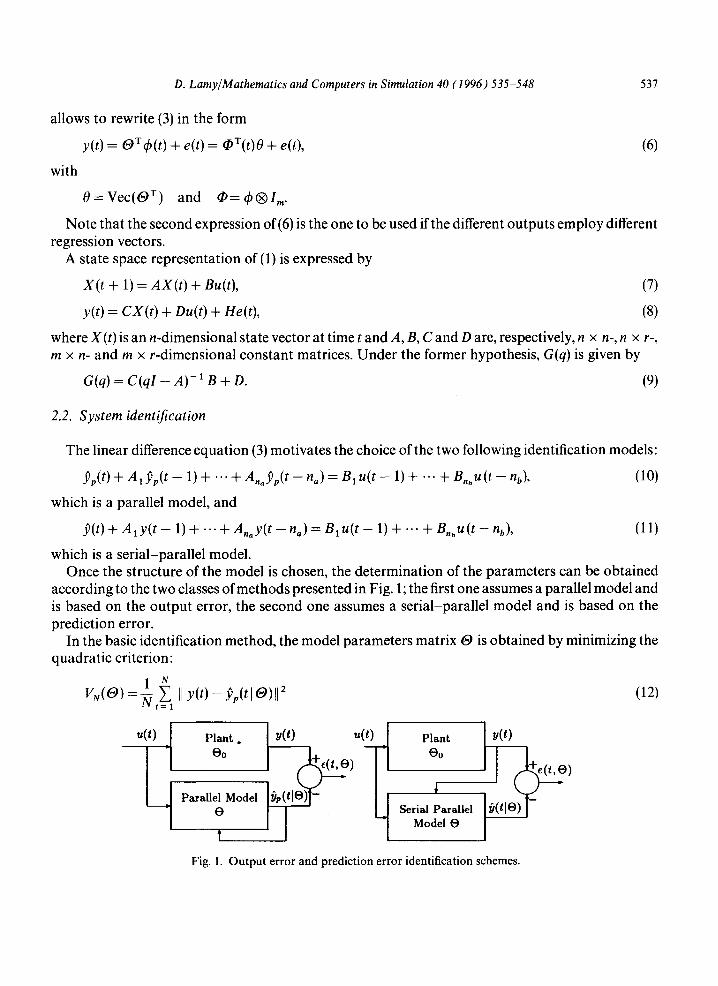
which is a serial-parallel model. Once the structure of the model is chosen, the determinat ion of the parameters can be obta ined

according to the two classes of me thods presented in Fig. 1; the first one assumes a parallel model and is based on the ou tpu t error, the second one assumes a serial-parallel model and is based on the predict ion error.

In the basic identification method , the model parameters matrix O is obtained by minimizing the quadrat ic criterion:

Fig. 1. Output error and prediction error identification schemes.

2.2. System identification

0 = V e c ( O T) and O = ~ b ® I , , .

Note that the second expression of(6) is the one to be used if the different outputs employ different regression vectors.

A state space representat ion of (1) is expressed by

S ( t + 1) = A X ( t ) + Bu(t), (7)

y(t) = CX( t ) + Du(t) + He(t), (8)

where X(t ) is an n-dimensional state vector at t ime t and A, B, C and D are, respectively, n × n-, n × r-, m × n- and m x r-dimensional constant matrices. Under the former hypothesis, G(q) is given by

G(q) = C(qI - A ) - 1 B + D. (9)


for the output error scheme, and

1 N VN(O) ---- ~ ,~1 II y(t) -- P(tl O)11 2 (13)

for the prediction error scheme. The output error identification scheme leads to the simulation model:

fip(tl 6)) = 6)T ~p(t, 6)), (14)

where the argument 6) in qSp(.) expresses the dependence of ~b~, on 6), so that the error e(t, 6))=y(t)-33p(t[6)) being nonlinear in parameters, nonlinear programming techniques or sensibility equations are needed to determine 6).

The prediction error identification scheme leads to the one step ahead predictor:

33(tl 6))-- 6)T~b(t), (15)

the error e(t, 6)) being linear in parameters, a least-squares criterion is used to determine 6). In (14) and (15), 6) and ~b(t) are defined as in (4) and (5), while ~p(t) is defined as ~b(t) with y(.)

replaced by 33,(.). The model (14) can be used for simulation purposes, e.g. evaluation of controllers under various design methods. The one step ahead predictor (15) can be used in adaptive control.

3. N e u r a l n e t w o r k s m o d e l s

3.1. Feedforward networks

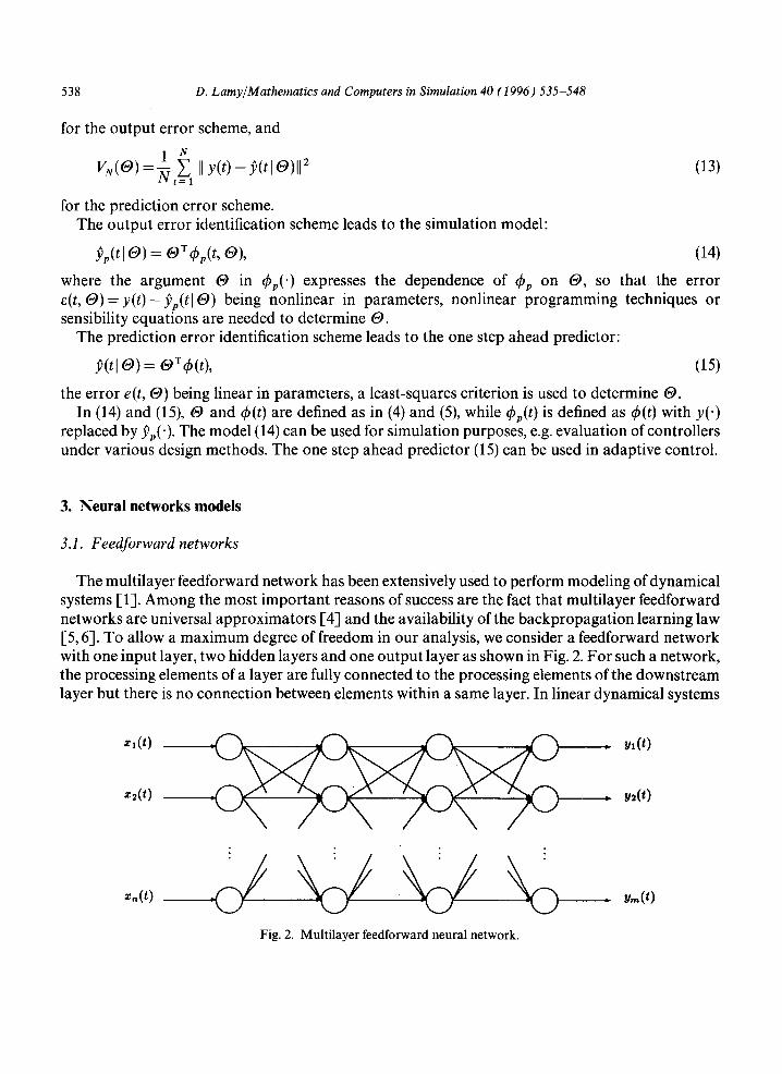
The multilayer feedforward network has been extensively used to perform modeling of dynamical systems I-1]. Among the most important reasons of success are the fact that multilayer feedforward networks are universal approximators [4] and the availability of the backpropagation learning law [5, 6-1. To allow a maximum degree of freedom in our analysis, we consider a feedforward network with one input layer, two hidden layers and one output layer as shown in Fig. 2. For such a network, the processing elements of a layer are fully connected to the processing elements of the downstream layer but there is no connection between elements within a same layer. In linear dynamical systems

Xl(t)

~2(t)

x,(t)

. v2(t)

Fig. 2. Multilayer feedforward neural network.

~,,(t)

D. Lamy/Mathematics and Computers in Simulation 40 (1996) 535 548 539

~,(t)

~(t)

x.(t)

. m( t ) z l ( t )

. y ~ ( t ) ~ 2 ( t )

: { wii } :

% x.(t) : . u,,,(t)

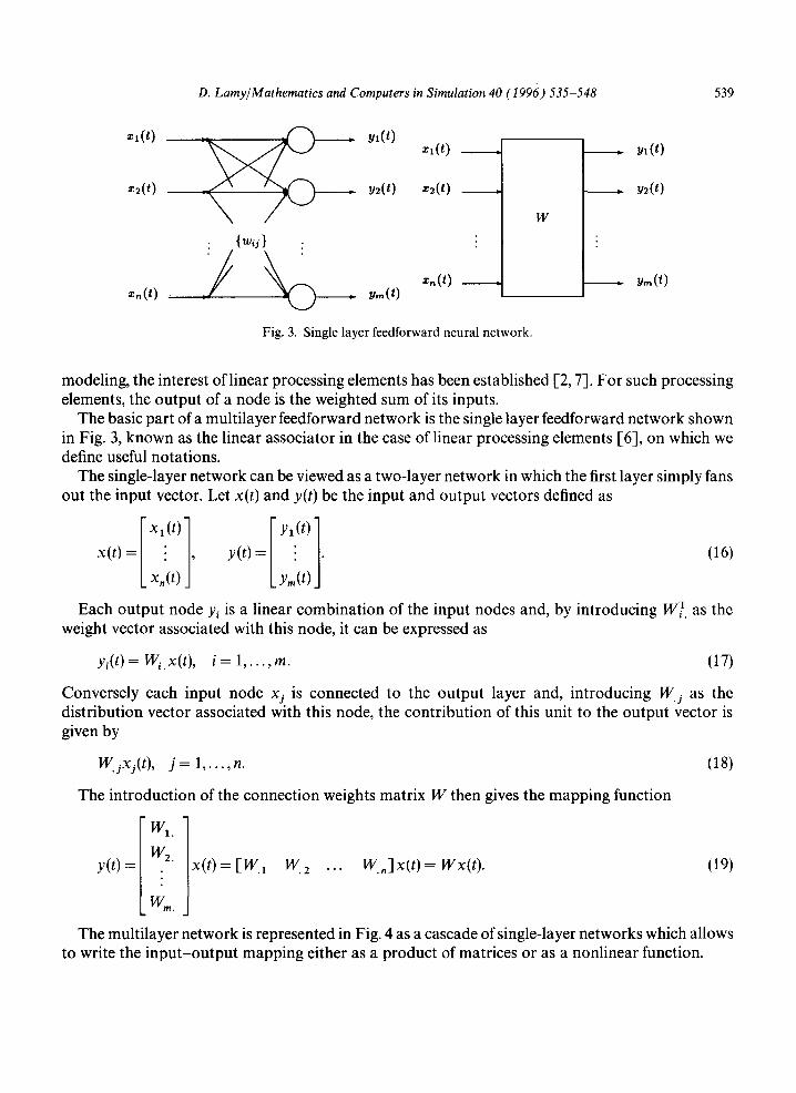
Fig. 3. Single layer feedforward neural network.

W

. y l ( t )

. u2 ( t )

. y = ( t )

modeling, the interest of linear processing elements has been established [2, 7]. For such processing elements, the output of a node is the weighted sum of its inputs.

The basic part of a multilayer feedforward network is the single layer feedforward network shown in Fig. 3, known as the linear associator in the case of linear processing elements [6], on which we define useful notations.

The single-layer network can be viewed as a two-layer network in which the first layer simply fans out the input vector. Let x ( t ) and y( t ) be the input and output vectors defined as

x ( t ) = " , y ( t ) = • . (16)

x , ( t ) Ly,,(t)

Each output node Yi is a linear combination of the input nodes and, by introducing W~ x. as the weight vector associated with this node, it can be expressed as

y , ( t ) = W , . x ( t ) , i = 1 . . . . . m . (17)

Conversely each input node xj is connected to the output layer and, introducing Wj as the distribution vector associated with this node, the contribution of this unit to the output vector is given by

Vf 4 x j ( t ) , j = 1 , . . . , n . (18)

The introduction of the connection weights matrix W then gives the mapping function

Wa

y( t ) = W2" x ( t ) = [W1 W2 ... W..]x(t) = W x ( t ) . (19)

w.

The multilayer network is represented in Fig. 4 as a cascade of single-layer networks which allows to write the inpu t -ou tpu t mapping either as a product of matrices or as a nonlinear function.

540 D. Lamy/ Mathematics and Computers in Simulation 40 (1996) 535-548

~,(t)

,2(t)

~,,(t)

~,x(t) _1

v,,,,]

'1 , ,~(t)

-I

W~

zl(t) I

~2(t) I

~ ( t )

;I

Ws

Fig. 4. Matrix notation for multilayer network.

, y~(i)

. u2( t )

. y , . ( t )

Let us introduce the vectors x(t), v(t), z(t) and y(t) defined as

x( t )= , v(t)= , z(t)= , y( t )= " , (20)

L .(oj L .(oj Lz (Oj y..(t)J being, respectively, the network input, first and second hidden, and output layers vectors. The first hidden layer realizes the mapping v ( t ) = W ix( t ) , the second hidden layer realizes the mapping z(t) = W2v( t ) and the output layer realizes the mapping y ( t ) = W3z(t). Therefore, the overall relationship of the network is given by

y(t) = W s z(t) = W s W z v(t) = W 3 W 2 W 1 x (t) = Wx( t ) , (21)

which is a linear mapping, and using the np + pq + qm neural net parameters vector On defined as

O.=[VecT(W,) VecV(Wz) Vecr(W3)] T, (22)

the neural network is defined by the nonlinear model

y(t , 6).) = 9 Ix ( t ) , 6).]. (23)

A multilayer feedforward network can be interpreted as a mapping network which implements an approximation of a function f : A c R n --. R m by means of training the weights of the connections on presentation of examples (x a, Y 1), (x2, Y z ) , . . . , (Xk, YR) of the mapping function where Yk =f(Xk)" When submitted to input x, the network realizes the mapping 9(x, On) where On is the vector composed of the network parameters. The accuracy of the network is measured by the square of the approximation error on presentation of the kth pattern namely F k = ]f(Xk) -- 9(Xk, 6).)12. On response to the presentation of N patterns, the backpropagation algorithm modifies the vector On in such a way that the mean squared error function F(6)n) defined as

1 N F(6)~) = lim _-: E Fk (24)

N ~ o o N k = l

is minimized.

D. Lamy/Mathematics and Computers in Simulation 40 (! 996) 535-548 541

3.2. Recurrent networks

A previous study [8] induced us into considering recurrent networks of the form presented in Fig. 5 for the neural implementation of canonical state space representations.

This network contains a row of fully interconnected neurons with connections comprising delays of one period. The components of the input command vector u(t) are fanned into every neuron. The outputs of the first neurons estimate the output vector of the process y(t + 1).

In a more general case, there could be a feedforward network instead of the unique row of neurons. As this network should be applied to linear processes identification, linear neurons which

compute a weighted sum of their inputs are used.

4. Neural identification

The multilayer feedforward network is used to implement the one step ahead predictor (15) ofy(t) according to Fig. 6.

outFuts

n e u r o n s

distribution units

delays

inputs ut(t)

yl(t+ I ) ... y,,(t+ I )

Fig. 5. Recurrent network.

I171

D

- p ( t - I)

-y ( t - 2)

: ] ~ - v ( t - .o)

,,(t - l)

: ~ ,,(t-.,)

Multilayer feed forward network O.

~(,le.)

Fig. 6. Neural predictor.


Intrinsically, a feedforward network does not have any dynamical memory. To enable a representation of dynamical systems it is thus associated with multiple delay lines.

The identification process is thus a learning one in which the network learns the mapping of regression vectors 4(t) into predicted outputs j(tl 0). For this purpose, past inputs and outputs of the plant are presented to the network; the actual output of the plant is used as a teaching signal to which the network output is compared. On the basis of the network output error, the backpropagation algorithm adapts the network weights vector 0,. The neural predictor is described by the model

9(4 0”) = sCM), @,I = w, w, w, 4(t) = wm, (25) and the prediction error is given by e(t, 0,) = y(t) - j(t, 0,).

Backpropagation implements a gradient steepest descent method, the parameters are updated along the negative gradient of F. The update is given by

0 rw = q- qF,;r(@,), (26)

which can be expressed, using the Kronecker product, as

(27)

The backpropagation algorithm is also known as the generalized delta rule for which the update, in the case of pattern update, is given by

W3(t + 1) = W3(t) + qe(t, O,)zT(t) (28)

for the output layer, in this expression e(t, 0,) is the prediction error,

W2(t + 1) = Wz(t) + q lVg(t)e(t, @,)uT(t)

‘for the second hidden layer,

W, (t + 1) = W,(t) + q w;(t) kVg(t)e(t, @.)x=(t)

for the first hidden layer.

(29)

(30)

Due to the increasing number of processing elements with input and output delays and dimensions, the learning phase is time consuming with random initial weights.

An alternative to the lack of dynamical capabilities of feedforward networks is to use the recurrent network of Fig. 5 which does have dynamical memory by itself. The number of external inputs neurons is reduced to the dimension of u(t), the number of internal neurons is given by the order of the process model. In that case, the learning law will be based on a variant of the backpropagation algorithm to modify the weights during identification [9].

5. Initialization and interpretation of neural models

The following sections indicate how the parameters of the two representations mentioned in Section 2 can be implemented on multilayered feedforwards and on recurrent neural networks. We explain, as well, how the functions computed by these networks can be modeled as transfer matrices and state space representations, in order to give an interpretation of neural models after training.

D. Lamy/Mathematics and Computers in Simulation 40 (1996) 535-548 543

5.1. Polynomial representation and feedforward networks

(1) Initialization. It has been shown that for a linear time invariant M I M O process model represented by the ARX model structure (3), the one step ahead predictor (15) can be implemented on a multilayer feedforward net with delay lines known as the neural predictor (25). Both predictor's expressions indicate that the multilayer net perfectly implements the model parameters matrix O provided we choose any W 1, W2, W 3 combination that satisfies the equality 0 x --- W 3 W 2 W 1.

We can profit by this degree of freedom to implement the a priori knowledge about structure and parameters values of a rough model of the process. The parameters of the one step ahead predictor (15) can be translated in the form of weights for the matrices WI, W z, W 3. This implementation may take various forms either concentrated or distributed.

(2) Interpretation. Conversely, as a multilayer feedforward realizes the mapping of input space vectors in output space vectors, once the weights have been fixed by learning, it can be interpreted as a one step ahead predictor provided that the input space is assumed to be the space of regression vectors, and the output space to be the space of predicted outputs. The model parameters matrix @ is then uniquely determined by I4"1, W 2, W 3.

5.2. State space representation and recurrent neural networks

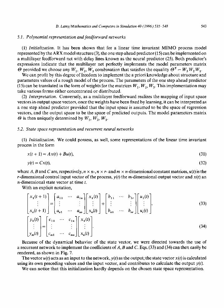
(1) Initialization. process in the form

x(t + 1) = Ax(t) + Bu(t),

y(t) = Cx(t),

We could possess, as well, some representations of the linear time invariant

(31)

(32)

where A, B and C are, respectively, n x n-, n x r- and m x n-dimensional constant matrices, u(t) is the r-dimensional control input vector of the process, y(t) the m-dimensional output vector and x(t) an n-dimensional state vector at time t.

With an explicit notation, [a,1 x . ( t ' + l ) - - a . l --. a . . j k x . ( t ) J bi l ... b,,JLu,(t) j

Ill 7 Yl(t) Cll "'" cl . xl(t)

• = " " ( 3 4 )

Ly,.(t)J " C . Lx.(t) J

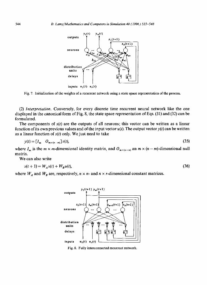
Because of the dynamical behavior of the state vector, we were directed towards the use of a recurrent network to implement the coefficients of A, B and C. Eqs. (33) and (34) can then easily be rendered, as shown in Fig. 7.

The vector u(t) acts as an input to the network, y(t) as the output; the state vector x(t) is calculated using its own preceding values and the input vector, and contributes to calculate the output y(t).

We can notice that this initialization hardly depends on the chosen state space representation•

544 D. LamyfMathematics and Computers in Simulation 40 (1996) 535-548

outputs

neurons

distribution units

delays

I I inputs u,(t) u,(l)

Fig. 7. Initialization of the weights of a recurrent network using a state space representation of the process.

(2) Interpretation. Conversely, for every discrete time recurrent neural network like the one displayed in the canonical form of Fig. 8, the state space representation of Eqs. (31) and (32) can be formulated.

The components of s(t) are the outputs of all neurons; this vector can be written as a linear function of its own previous values and of the input vector u(t). The output vector y(t) can be written as a linear function of s(t) only. We just need to take

Y(t) = Kfl e?Ix(n-mJS@), (35)

where I, is the m x m-dimensional identity matrix, and 0, x+mJ an m x (n - m)-dimensional null matrix.

We can also write

s(t + 1) = IV‘&) + W&J(t),

where WA and IV, are, respectively, n x n- and n x r-dimensional constant matrices.

(36)

Y*(l+l) Y,(r+l) oulputs

neurons

distribution units

delays

inputs

Fig. 8. Fully interconnected recurrent network.

D. Lamy/Mathematics and Computers in Simulation 40 (1996) 535-548 545

Eqs. (36) and (35) belong to the classes of Eqs. (31) and (32). The state vector x(t) in Eqs. (31) and (32) is represented by s(t) in Eqs. (35) and (36), and the constant matrices A, B and C in Eqs. (31) and (32) are replaced by the particular forms WA, W B and [1., O.,×¢,-mt] in Eqs. (35) and (36).

So, in the first place, the results of the former section provide a method to guide the initialization of neural nets applied to linear time invariant process identification, and in the second place, these last expressions allow us to interpret and to check the networks manipulated after a training period.

6. Sensitivity analysis of neural models

On the major constraints of the backpropagation learning are the time consuming adaptation of weights and lack of information to give the network an adequate dimension. To remedy the first problem, it appears then important to start the learning procedure with a good initial weights vector. One method to realize this goal is to use a priori information available on the process parameters to initialize the network parameters vector @n. One question then arises: does there exist a better way to distribute the available information on the weights of the network? The response to this question arises from the considerations of sensitivity functions or vector norms. Assuming that the regression model (15) as well as the neural predictor (25) give the parameters of the ARX model (3), it is then reasonable to write the equality between the two models by

oT~b(t) = gl-~b(t), On] = W 3 W 2 Wick(t)= Wc~(t), (37)

where the parameter matrix @ clearly appears as a nonlinear function of the neural network weights and, using definition (22) of @n, and the properties of the Kronecker product is given by

Vec(@ T) = (In ® (W3 W2)) Vec(W1) = (W~ ® Wa)Vec(W2) = ((W 2 W~) x @ I,,)Vec(W3). (38)

This expression will allow us to evaluate the sensitivity of the ARX parameters versus neural predictor parameters and the robustness of the neural model versus the weights vector.

A response to the second problem is immediate by considering the sensitivity of the neural predictor output p(t, @n) to the weight vector @n. This sensitivity function permits to locate the connections with minor influence. A pruning procedure is then established to give the network the smallest possible dimension.

6.1. Robustness of the A R X model versus weights vector

As a lot of weights combinations are susceptible to implement correctly the ARX model structure, the sensitivity function @~n is useful to select the optimal neural weights vector which ensures the maximum robustness of ARX parameters versus neural parameters.

6.2. Robustness of neural model versus weights vector

By using a two-phase training, we will determine the neural weights vector which ensures the maximum robustness of the neural model versus neural weights vector. In the first phase the simple backpropagation algorithm is used to find a near optimal weights vector, the procedure is stopped


when the mean square error criterion is sufficiently small. In the second phase, the criterion to minimize is modified such that

F k = e(t, ~gn)Te(t, On) + g I[ J)o~ II, (39)

the second component of the criteria is interpreted as a penalty term. A new training procedure is then started from the previously attained weights vector which, for small value of ~, forces the neural parameters vector to slide towards a real minimum.

6.3. Determination of network dimension

The contribution of each neuron of the network to the predicted output calculated by the network is determined by evaluating the maximum contribution of this neuron over all possible values of its distribution vector:

AT max Yw~,, (40) I W!k [ < W!kmax

where Wt.k represents the distribution vector associated with the neuron numbered k in the / th layer and Wt.k max represents the distribution vector when all its weights are at their maximum values.

The least influencing neuron is then determined and removed. A new training procedure is started, if the criterion is small enough the pruning process is pursued else it is stopped and the results of the preceeding step are retained.

7. Conclusion

Neural networks models are given for the implementation of polynomial and state space forms of the transfer function of MIMO linear process. It is discussed how to use some a priori knowledge about structure and parameters values of the process model to initialize the neural nets. The adaptation of the neural model is written in a simple form for the case of linear processing units. Finally, some sensitivity functions used to ensure robustness of the neural model and to give the network an adequate dimension are presented.

Acknowledgements

This work was supported by the F6d6ration Universitaire et Polytechnique de Lille, the FEDER and the Conseil R6gional Nord Pas de Calais.

Appendix A. Matrices notations and definitions

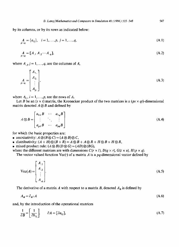
We introduce here the notations used in matrix manipulation as well as the definition and properties of the Kronecker product [ 10-1. A (p × q)-dimensional matrix A is defined by its elements,

D. Lamy/Mathematics and Computers in Simulation 40 (1996) 535-548

by its columns, or by its rows as indicated below:

A ={ai j } , i = 1 . . . . . p , j = l , . . . , q , pxq

547

(A.1)

A = [A.1 A.2 . . . A . q ] , (A.2) p×q

where A. j, j = 1 . . . . , q, are the columns of A,

A I

A = A2 p×q

Ap

(A.3)

where Ai., i = 1, . . . , p, are the rows of A. Let B be an (s x t) matrix, the Kronecker product of the two matrices is a (ps x qt)-dimensional

matrix denoted A @ B and defined by

I a l l B ".. a lqB

A Q B = " . . "

apl B ... apqB

(A.4)

for which the basic properties are: • associativity: A ® (B @ C) = (A @ B) @ C, • distributivity: (A + H) @ (B + R) = A ® B + A ® R + H ® B + H ® R, • mixed product rule: (A ® B) (D @ G) = (AD) ® (BG), where the different matrices are with dimensions C(r x l), D(q x r), G(t x u), H ( p x q).

The vector valued function Vec(.) of a matrix A is a pq-dimensional vector defined by

Vec(A) = [i 1] Z'2 .

q

(A.5)

The derivative of a matrix A with respect to a matrix B, denoted A B is defined by

A B = ~3BTA (A.6)

and, by the introduction of the operational matrices

a--B = ~ aA = [aa,j ] , (A.7)

548 D. LamyjMathematics and Computers in Simulation 40 (1996) 535-548

the differential operation A, is written as

A, = ( l/dBT) @ dA. (A.81 Finally, I, is the (m x m)-dimensional identity matrix.

References

[l] K.S. Narendra and K. Parthasarathy, Identification and control of dynamical systems using neural networks, IEEE Trans. Neural Networks l(l990) 4-27.

[2] D.T. Pham and X. Liu, Neural networks for discrete dynamic system identification, J. System Engrg. l(l991) 51-60. [3] L. Ljung, System Identification: Theory for the User (Prentice-Hall, Englewood Cliffs, NJ, 1987). [4] K. Hornik, M. Stinchcombe and H. White, Multilayer feedforward networks are universal approximators, Neural

Networks 2 (1989) 359-366. [S] D.E. Rumelhart and J.L. McClelland, Parallel Distributed Processing: Explorations in the Microstructure of

Cognition (MIT Press, Cambridge, MA, 1986). [6] R. Hecht-Nielsen, Neurocomputing (Addison-Wesley, Reading, MA, 1989). [7] B. Widrow and S. Stearns, Adaptive Signal Processing (Prenctice-Hall, Englewood Cliffs, NJ, 1985). [8] M. Decotte, Propositions pour l’initialisation de reseaux de neurones destines a l’identification, Mtmoire de DEA,

Universite des Sciences et Techniques de Lille-Flandres-Artois, France, July 1992. [9] P.J. Werbos, Generalization of backpropagation with application to a recurrent gas market model, Neural Networks

1 (1988) 339-356. [lo] F. Rotella, Improvements on derivatives of matrices, J. Franklin Institute 328(4) (1991) 487-503.

modeling and sensitivity analysis of neural networks

Documents