modeling and estimation of phase noise in oscillators with...

Modeling and Estimation of Phase Noise

in Oscillators with Colored Noise Sources

M. Reza Khanzadi

Communication Systems GroupDepartment of Signals and SystemsMicrowave Electronic LaboratoryDepartment of Microtechnology and NanoscienceCHALMERS UNIVERSITY OF TECHNOLOGY

Göteborg, Sweden

THESIS FOR DEGREE OF LICENTIATE OF ENGINEERING

Modeling and Estimation of Phase Noise

in Oscillators with Colored Noise Sources

M. Reza Khanzadi

Communication Systems GroupDepartment of Signals and Systems

Microwave Electronic LaboratoryDepartment of Microtechnology and Nanoscience

Chalmers University of Technology

Göteborg, August 2013

Khanzadi, M. RezaModeling and Estimation of Phase Noise in Oscillators with Colored Noise Sources

Technical Report No. R019/2013ISSN 1403-266X

Communication Systems GroupDepartment of Signals and SystemsChalmers University of TechnologySE-412 96 Göteborg, SwedenTelephone: + 46 (0)31-772 1000

Microwave Electronic LaboratoryDepartment of Microtechnology and NanoscienceChalmers University of TechnologySE-412 96 Göteborg, SwedenTelephone: + 46 (0)31-772 1000

Copyright ©2013 M. Reza Khanzadiexcept where otherwise stated.All rights reserved.

Homepage: http://khanzadi.infoEmail: [email protected]

This thesis has been prepared using LATEX.

Front Cover : The figure on the front cover is the distorted received signal constellation of a 16-QAMcommunication system due to transmitter and receiver oscillator phase noise.

Printed by Chalmers Reproservice,Göteborg, Sweden, August 2013.

ABSTRACT

The continuous increase in demand for higher data rates due to applications with massivenumber of users motivates the design of faster and more spectrum efficient communi-cation systems. In theory, the current communication systems must be able to operateclose to Shannon capacity bounds. However, the real systems perform below capacitylimits, mainly due to channel estimation error and hardware impairments that have beenneglected by idealistic or simplistic assumptions on the imperfections.

Oscillator phase noise is one of the hardware impairments that is becoming a limitingfactor in high data rate digital communication systems. Phase noise severely limits theperformance of systems that employ dense constellations. Moreover, the level of phasenoise (at a given off-set frequency) increases with carrier frequency which means that theproblem of phase noise may be even more severe in systems with high carrier frequency.

The focus of this thesis is on finding accurate statistical models of phase noise, aswell as the design of efficient algorithms to mitigate the effect of this phenomenon on theperformance of modern communication systems. First we derive the statistics of phasenoise with white and colored noise sources in free-running and phase-locked-loop-stabilizedoscillators. We investigate the relation between real oscillator phase noise measurementsand the performance of communication systems by means of the proposed model. Ourfindings can be used by hardware and frequency generator designers to better understandthe effect of phase noise with different sources on the system performance and optimizetheir design criteria respectively.

Then, we study the design of algorithms for estimation of phase noise with colorednoise sources. A soft-input maximum a posteriori phase noise estimator and a modifiedsoft-input extended Kalman smoother are proposed. The performance of the proposedalgorithms is compared against that of those studied in the literature, in terms of meansquare error of phase noise estimation, and symbol error rate of the considered com-munication system. The comparisons show that considerable performance gains can beachieved by designing estimators that employ correct knowledge of the phase noise statis-tics. The performance improvement is more significant in low-SNR or low-pilot densityscenarios.

Keywords: Oscillator Phase Noise, Voltage-controlled Oscillator, Phase-Locked Loop,Colored Phase Noise, Phase Noise Model, Bayesian Cramér-Rao Bound, Maximum aPosteriori Estimator, Extended Kalman Filter/Smoother, Mean Square Error.

i

LIST OF PUBLICATIONS

Appended papersPaper AM. Reza Khanzadi, Dan Kuylenstierna, Ashkan Panahi, Thomas Eriksson, and Her-bert Zirath, "Calculation of the Performance of Communication Systems from MeasuredOscillator Phase Noise," Accepted for publication in IEEE Transactions on Circuits andSystems I, Aug. 2013.

Paper BM. Reza Khanzadi, Rajet Krishnan, and Thomas Eriksson, "Estimation of Phase Noisein Oscillators with Colored Noise Sources," Accepted for publication in IEEE Communi-cations Letters, Aug. 2013.

Other publications[J1] Rajet Krishnan, M. Reza Khanzadi, Thomas Eriksson, and Tommy Svensson,"Soft metrics and their Performance Analysis for Optimal Data Detection in the Presenceof Strong Oscillator Phase Noise," IEEE Transactions on Communications, Jun. 2013.

[J2] Hani Mehrpouyan, M. Reza Khanzadi, Michail Matthaiou, Robert Schober, andYingbo Hua, "Improving Bandwidth Efficiency in E-band Communication Systems," Sub-mitted to IEEE Communications Magazine, Sep. 2012.

[C1] M. Reza Khanzadi, Rajet Krishnan, and Thomas Eriksson,"Effect of SynchronizingCoordinated Base Stations on Phase Noise Estimation," IEEE Conference on Acoustic,Speech, and Signal Processing (ICASSP), May. 2013.

[C2] M. Reza Khanzadi, Ashkan Panahi, Dan Kuylenstierna, and Thomas Eriksson,"A model-based analysis of phase jitter in RF oscillators," IEEE International FrequencyControl Symposium (IFCS), May. 2012.

iii

[C3] Rajet Krishnan, M. Reza Khanzadi, Lennart Svensson, Thomas Eriksson, andTommy Svensson, "Variational Bayesian Framework for Receiver Design in the Presenceof Phase Noise in MIMO Systems," IEEE Wireless Communications and Networking Con-ference (WCNC), Apr. 2012.

[C4] M. Reza Khanzadi, Hani Mehrpouyan, Erik Alpman, Tommy Svensson, DanKuylenstierna, and Thomas Eriksson,"On models, bounds, and estimation algorithms fortime-varying phase noise,"IEEE International Conference on Signal Processing and Com-munication Systems (ICSPCS), Dec. 2012.

[C5] M. Reza Khanzadi, Kasra Haghighi, and Thomas Eriksson, "Optimal Modulationfor Cognitive Transmission over AWGN and Fading Channels,"IEEE European WirelessConference, Apr. 2011.

[C6] M. Reza Khanzadi, Kasra Haghighi, Ashkan Panahi, and Thomas Eriksson, "ANovel Cognitive Modulation Method Considering the Performance of Primary User," IEEEWireless Advanced Conference (WiAD) Jun. 2010.

[C7] Arash Toyserkani, M. Reza Khanzadi, Erik Ström, and Arne Svensson, "A Com-plexity Adjustable Scheduling Algorithm for Throughput Maximization in ClusterizedTDMA Networks,"IEEE Vehicular Technology Conference (VTC), May. 2010.

ACKNOWLEDGEMENTS

Doing a PhD is a journey to the unknown! You do not know where to start and yourdestination may not be clearly known either! On such a journey the last thing you needis to be alone. It is always the support and help of the people around you, which makesyou feel Passionate, hopeful, and Developing on this journey.

Now in the middle of this journey I would like to express my deepest gratitude to mysupervisor Prof. Thomas Eriksson who has always supported me with his sharp insightand invaluable feedback. Thomas, you have always been my best source of motivation.My greatest gratitude also goes to my examiner Prof. Herbert Zirath for his generoussupport. I hope I can learn more and more from you during the rest of my PhD. I wouldalso like to offer my special thanks to my co-supervisor and my sport hero Dr. DanKuylenstierna for all his constructive comments and warm encouragement. I really enjoyour discussions and look forward to more of those and further possibilities of learningfrom you. My appreciation also goes to Prof. Erik Ström for giving me the opportunityto be a part of ComSys family.

Special thanks to Rajet Krishnan, my research buddy and a great officemate, for allfruitful discussions we have. As experience has shown the Thomas-Reza-Rajet trianglerocks in writing papers! Let’s keep it up! I also need to thank Dr. Hani Mehrpouyan,who made me more interested in estimation theory and for all his support during his stayin Sweden. And finally my friend Ashkan Panahi, I learned from you how to tackle aproblem. Thanks for all intensive discussions inside and outside the university.

Former and current colleagues at S2 and MC2, and my friends

Agneta

Madeleine

thank you for being there and supporting me.

v

My sincerest gratitude goes to my family and their never-ending support. Shirin,Shohreh, and Giti, thank you for everything.

Last but not least, my beloved Fatemeh, you have always been there for me in all thetears and laughs of this PhD life! Thank you for your love, support and patience. Youare the only one from management world who knows a lot about oscillator phase noisenow!

M. Reza KhanzadiGöteborg August 2013

CONTENTS

Abstract i

List of Publications iii

Acknowledgements v

Acronyms ix

I Introduction 1

1 Overview 11 Introduction . . . . . . . . . . . . . . . . . . . . . . . . . . . . . . . . . . 12 Aim of the Thesis . . . . . . . . . . . . . . . . . . . . . . . . . . . . . . . 23 Thesis Outline . . . . . . . . . . . . . . . . . . . . . . . . . . . . . . . . . 2

2 Communication System Model 31 Practical Communication Systems . . . . . . . . . . . . . . . . . . . . . . 32 Model of the Received Signal . . . . . . . . . . . . . . . . . . . . . . . . 43 Effect of Phase Noise on Communication Systems . . . . . . . . . . . . . 5

3.1 Rotation of the Constellation Diagram . . . . . . . . . . . . . . . 53.2 Spectral Regrowth . . . . . . . . . . . . . . . . . . . . . . . . . . 6

3 Phase Noise in Oscillators 71 Oscillators . . . . . . . . . . . . . . . . . . . . . . . . . . . . . . . . . . . 72 Phase Noise in Oscillators . . . . . . . . . . . . . . . . . . . . . . . . . . 73 Phase Noise Generation . . . . . . . . . . . . . . . . . . . . . . . . . . . 94 Phase Noise Modeling . . . . . . . . . . . . . . . . . . . . . . . . . . . . 10

4.1 Variance of the White Phase Noise Process . . . . . . . . . . . . . 124.2 Statistics of the Cumulative PN Increments . . . . . . . . . . . . 13

4 Phase Noise Compensation 151 Overview . . . . . . . . . . . . . . . . . . . . . . . . . . . . . . . . . . . . 152 Bayesian Framework . . . . . . . . . . . . . . . . . . . . . . . . . . . . . 16

vii

2.1 Bayesian Estimation . . . . . . . . . . . . . . . . . . . . . . . . . 162.2 Estimation of Phase Noise with Colored Noise Sources . . . . . . 16

3 Performance of Bayesian Estimators . . . . . . . . . . . . . . . . . . . . . 173.1 Bayesian Cramér Rao Bound . . . . . . . . . . . . . . . . . . . . 17

5 Conclusions, Contributions, and Future Work 181 Conclusions . . . . . . . . . . . . . . . . . . . . . . . . . . . . . . . . . . 182 Contribution . . . . . . . . . . . . . . . . . . . . . . . . . . . . . . . . . . 183 Future Work . . . . . . . . . . . . . . . . . . . . . . . . . . . . . . . . . . 19References . . . . . . . . . . . . . . . . . . . . . . . . . . . . . . . . . . . . . . 20

II Included papers 25

A Calculation of the Performance of Communication Systems from Mea-sured Oscillator Phase Noise A11 Introduction . . . . . . . . . . . . . . . . . . . . . . . . . . . . . . . . . . A22 System Model . . . . . . . . . . . . . . . . . . . . . . . . . . . . . . . . . A3

2.1 Phase Noise Model . . . . . . . . . . . . . . . . . . . . . . . . . . A42.2 Communication System Model . . . . . . . . . . . . . . . . . . . . A6

3 System Performance . . . . . . . . . . . . . . . . . . . . . . . . . . . . . A83.1 Background: Cramér-Rao bounds . . . . . . . . . . . . . . . . . . A83.2 Calculation of the bound . . . . . . . . . . . . . . . . . . . . . . . A93.3 Calculation of Error Vector Magnitude . . . . . . . . . . . . . . . A10

4 Phase Noise Statistics . . . . . . . . . . . . . . . . . . . . . . . . . . . . A114.1 Calculation of σ2

φ0 . . . . . . . . . . . . . . . . . . . . . . . . . . . A124.2 Calculation of Rζ3 [m] and Rζ2 [m] . . . . . . . . . . . . . . . . . . A12

5 Numerical and Measurement Results . . . . . . . . . . . . . . . . . . . . A145.1 Phase Noise Simulation . . . . . . . . . . . . . . . . . . . . . . . . A145.2 Monte-Carlo Simulation . . . . . . . . . . . . . . . . . . . . . . . A155.3 Analysis of the Results . . . . . . . . . . . . . . . . . . . . . . . . A165.4 Measurements . . . . . . . . . . . . . . . . . . . . . . . . . . . . . A19

6 Conclusions . . . . . . . . . . . . . . . . . . . . . . . . . . . . . . . . . . A197 Appendix A . . . . . . . . . . . . . . . . . . . . . . . . . . . . . . . . . . A218 Appendix B . . . . . . . . . . . . . . . . . . . . . . . . . . . . . . . . . . A22References . . . . . . . . . . . . . . . . . . . . . . . . . . . . . . . . . . . . . . A26

B Estimation of Phase Noise in Oscillators with Colored Noise Sources B11 Introduction . . . . . . . . . . . . . . . . . . . . . . . . . . . . . . . . . . B22 System Model . . . . . . . . . . . . . . . . . . . . . . . . . . . . . . . . . B23 Phase Noise Estimation . . . . . . . . . . . . . . . . . . . . . . . . . . . B3

3.1 Proposed MAP Estimator . . . . . . . . . . . . . . . . . . . . . . B33.2 Auto Regressive Model of Colored Phase Noise Increments . . . . B5

4 Numerical Results . . . . . . . . . . . . . . . . . . . . . . . . . . . . . . . B75 Conclusions . . . . . . . . . . . . . . . . . . . . . . . . . . . . . . . . . . B96 Appendix . . . . . . . . . . . . . . . . . . . . . . . . . . . . . . . . . . . B9References . . . . . . . . . . . . . . . . . . . . . . . . . . . . . . . . . . . . . . B11

ACRONYMS

ADC: Analog to Digital Converter

AR: Autoregressive

AWGN: Additive White Gaussian Noise

BCRB: Bayesian Cramér-Rao Bound

BER: Bit Error Rate

BIM: Bayesian Information Matrix

CRB: Cramér-Rao Bound

EKS: Extended Kalman Smoother

EVM: Error-Vector Magnitude

FIM: Fisher Information Matrix

GaN: Gallium Nitride

HEMT: High-Electron-Mobility Transistor

I/Q: Inphase / Quadrature Phase

LNA: Low-Noise Amplifier

MAP: Maximum a Posteriori

MBCRB: Modified Bayesian Cramér-Rao Bound

MIMO: Multiple-Input Multiple-Output

ML: Maximum Likelihood

MMIC: Monolithic Microwave Integrated Circuit

MMSE: Minimum Mean Square Error

MSE: Mean Squared Error

OFDM: Orthogonal Frequency Division Multiplexing

ix

PA: Power Amplifier

PDF: Probability Density Function

PLL: Phase-Locked Loop

PN: Phase Noise

PSD: Power Spectral Density

QAM: Quadrature Amplitude Modulation

RF: Radio Frequency

SER: Symbol Error Rate

SNR: Signal-to-Noise Ratio

SSB: Single-Side-Band

Part I

Introduction

CHAPTER 1

OVERVIEW

1 Introduction

Digital communication has become an indispensable part of our personal and professionallives. Data transmission rates over fixed and wireless networks have been increasingrapidly due to applications with massive number of users such as smartphones, tablets,wired and wireless broadband Internet connections, cloud computing, the machine-to-machine communication services, etc. Demands for higher data rates continue to increaseat about 60% per year [1].

This increasing demand motivates the need for design of faster and more spectrum effi-cient communication systems. Despite the progress in theoretical aspects of such systems,the analog front end still fails to deliver what is promised mainly due shortcomings suchas hardware impairments. Hardware impairments in radio-frequency and optical commu-nications, such as amplifier nonlinearity, IQ imbalance, optical channel nonlinearities, andoscillator or laser phase noise, can be seen as the bottlenecks of the performance [2].

A promising solution to overcome this problem is to mitigate the effects of hardwareimpairments by means of digital signal processing algorithms. A key step in this avenueis to find mathematical models that can accurately represent the physical impairments.In many prior studies, simple models have been employed for this purpose. For instance,using the additive white Gaussian noise has been a normal practice to summarize all un-wanted effects from communication channel and hardware components on the transmittedsignal. However, to be able to come up with efficient algorithms, better understandingand modeling of the hardware impairments is needed.

Oscillator phase noise (PN) is one of the hardware imperfections that is becoming alimiting factor in high data rate digital communication systems. PN severely limits theperformance of systems that employ dense constellations. The negative effect of phasenoise is more pronounced in high carrier frequency systems, e.g., E-band (60-80 GHz),mainly due to the high level of PN in oscillators designed for such frequencies [3–5].Moreover, PN severely affects the performance of multiple antenna (MIMO) systems [6,7],and also destroys the orthogonality of the subcarriers in orthogonal frequency divisionmultiplexing (OFDM) systems that degrades the performance by producing intercarrierinterference [8, 9].

2 Overview

In many prior studies, PN is modeled as a discrete random walk with uncorrelated(white) Gaussian increments between each time instant (i.e., the discrete Wiener process).This model results from using oscillators with white noise sources [10]. However, numerousstudies show that real oscillators also contain colored noise sources [10–15].

In summary, accurate PN models and efficient algorithms to mitigate the effect of thisphenomenon are central to the design of modern communication systems. These aspectsform the core of this thesis.

2 Aim of the ThesisIn this thesis, we focus on three important aspects of dealing with PN in communicationsystems:

• We provide an accurate statistical model for PN in practical oscillators. This modelcan further be used for accurate simulations of PN-affected communication systems,as well as design of algorithms for compensation of PN.

• We calculate the performance of a PN-affected communication system from givenoscillator’s PN measurements. Such results can have important effects on design ofhardware for frequency generation.

• We design and implement PN estimation algorithms by employing our proposedstatistical model. We show that considerable performance improvements can beachieved by using the proposed algorithms, especially in low signal-to-noise ratio(SNR) and low-pilot-density scenarios.

3 Thesis OutlineWe start the Chapter 2 of this thesis by explaining different sources of hardware im-pairments in practical communication systems. Then we focus on PN and describe itseffects by introducing a mathematical model for a PN-affected communication system.In Chapter 3, we talk about oscillators, their roles in communication systems, and thesources of PN in oscillators. Further, we propose a new statistical model for the PN ofreal oscillators. In Chapter 5, we focus on design of algorithms for PN compensation. Wedescribe the basics of Bayesian estimation theory and finish the chapter by describing thebounds on the performance of such estimators. Finally, we summarize our contributionsin Chapter 6.

CHAPTER 2

COMMUNICATION SYSTEM MODEL

1 Practical Communication Systems

Hardware impairments are an inevitable consequence of using non-ideal components incommunication systems. Any practical communication system consists of several com-ponents that play a specific role in the transmission of data stream from one point toanother. Fig. 2.1 illustrates a simplified hardware block diagram of a typical wirelesscommunication system.

PA

LNA

DAC

ADC

LocalOscillator

LocalOscillator Antenna

Antenna

DigitalSignalProcessing

Mixer

Mixer

Data (bits)

Data (bits)

Transmitter

Receiver

Unit

DigitalSignalProcessingUnit

RF

RF

Baseband

Baseband

Figure 2.1: Hardware block diagram of the transmitter and receiver in a typicalcommunication system.

All the system components are made of electronic devices such as resistors, inductors,capacitors, diodes, and transistors, which are composed of conductor and semiconductormaterials. These electronic devices are not perfect and can behave differently from what

4 Communication System Model

is predicted for many reasons such as temperature variation, aging, pressure, etc.One of the major hardware impairments affecting the performance of communication

systems is oscillator PN. Oscillators are one of the main building blocks in a communi-cation system. Their role is to create stable reference signals for frequency and timingsynchronization. Unfortunately, any real oscillator suffers from hardware imperfectionsthat introduce PN to the communication system. The fundamental source of the PN isthe inherent noise of the passive and active components (e.g., thermal noise) inside theoscillator circuitry [11, 16].

2 Model of the Received SignalConsider a single-carrier single-antenna communication system. The transmitted signalx(t) is

x(t) =N∑

n=1s[n]p(t − nT ), (2.1)

where s[n] denotes the modulated symbol from constellation C with an average sym-bol energy of Es, n is the transmitted symbol index, p(t) is a bandlimited square-rootNyquist shaping pulse function with unit-energy, and T is the symbol duration [17]. Thecontinuous-time complex-valued baseband received signal after down-conversion, affectedby the transmitter and receiver oscillator PN, can be written as

r(t) = x(t)ejφ(t) + w(t), (2.2)

where φ(t) denotes the PN process and w(t) is zero-mean circularly symmetric complex-valued additive white Gaussian noise (AWGN), that models the effect of noise from othercomponents of the system. The received signal (2.2) is passed through a matched filterp∗(−t) and the output is

y(t) =∫ ∞

−∞

N∑n=1

s[n]p(t − nT − τ)p∗(−τ)ejφ(t−τ)dτ

+∫ ∞

−∞w(t − τ)p∗(−τ)dτ. (2.3)

Assuming PN does not change over the symbol duration, but changes from one symbolto another so that no intersymbol interference arises, sampling the matched filter output(2.3) at nT time instants results in

y(nT ) = s[n]ejφ(nT ) + w(nT ). (2.4)

We change the notation as

y[n] = s[n]ejφ[n] + w[n], (2.5)

where φ[n] represents the PN of the nth received symbol in the digital domain that isbandlimited after the matched filter, and w[n] is the filtered (bandlimited) and sampledversion of w(t) that is a zero-mean circularly symmetric complex-valued AWGN with

3 Effect of Phase Noise on Communication Systems 5

variance σ2w. Note that in this work our focus is on oscillator phase synchronization and

time synchronization is assumed to be perfect.The slow varying PN assumption and the introduced discrete-time model (2.5), are

well accepted in related literature (e.g., [8,9,18–30]). We also refer the reader to the recentstudies of this model where the PN variations over the symbol period has also been takeninto consideration, and the possible loss due to the slow varying PN approximation hasbeen investigated [31–33].

3 Effect of Phase Noise on Communication SystemsAs we saw in the previous section in Eq. 2.5, PN destroys the transmitted signals. Randomrotation of the received signal constellation [18, 22, 30], and spectrum regrowth [8, 9, 20,23, 34] are the main effects of this phenomenon on the communication systems.

3.1 Rotation of the Constellation Diagram

PN results in random rotation of the received signal constellation, which in phase modu-lated transmissions may lead to symbol detection errors [18, 22, 30].

Fig. 2.2a illustrates the received signal constellation of a system employing 16-QAMmodulation format over an AWGN channel. Fig. 2.2b, on the other hand shows the effectof PN from a free-running oscillator on the received signal constellation. The rotatorydistortions are due to the random variation of the phase of the received signal. The dashedlines show the Voronoi regions of a coherent detector, designed for the AWGN channel.PN cause decision errors by moving the received signals to wrong decision regions.

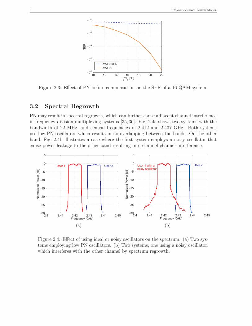
Fig. 2.3 shows the effect of PN before compensation on symbol error rate (SER) ofthe system, where it is compared against the SER in case of AWGN.

-1.5 -1 -0.5 0 0.5 1 1.5-1.5

-1

-0.5

0

0.5

1

1.5

In-Phase

Quadrature

(a)

-1.5 -1 -0.5 0 0.5 1 1.5-1.5

-1

-0.5

0

0.5

1

1.5

In-Phase

Quadrature

(b)

Figure 2.2: Received signal constellation of a 16-QAM system. (a) Pure AWGNchannel with SNR=25 dB. (b) AWGN channel affected by PN, SNR=25 dB andPN increment variance of 10−4 rad2/symbol duration.

6 Communication System Model

10 12 14 16 18 20 2210

-8

10-6

10-4

10-2

100

Es/N

o[dB]

SE

R

AWGN+PN

AWGN

Figure 2.3: Effect of PN before compensation on the SER of a 16-QAM system.

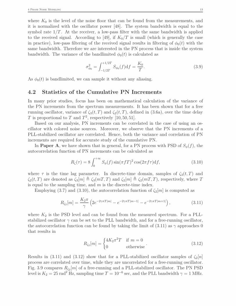
3.2 Spectral RegrowthPN may result in spectral regrowth, which can further cause adjacent channel interferencein frequency division multiplexing systems [35,36]. Fig. 2.4a shows two systems with thebandwidth of 22 MHz, and central frequencies of 2.412 and 2.437 GHz. Both systemsuse low-PN oscillators which results in no overlapping between the bands. On the otherhand, Fig. 2.4b illustrates a case where the first system employs a noisy oscillator thatcause power leakage to the other band resulting interchannel channel interference.

2.4 2.41 2.42 2.43 2.44 2.45-30

-25

-20

-15

-10

-5

0

5

Frequency [GHz]

Norm

alized P

ow

er

[dB

]

User 1 User 2

(a)

2.4 2.41 2.42 2.43 2.44 2.45-30

-25

-20

-15

-10

-5

0

5

Frequency [GHz]

Norm

alized P

ow

er

[dB

]

User 1 with a

noisy oscillator

User 2

(b)

Figure 2.4: Effect of using ideal or noisy oscillators on the spectrum. (a) Two sys-tems employing low PN oscillators. (b) Two systems, one using a noisy oscillator,which interferes with the other channel by spectrum regrowth.

CHAPTER 3

PHASE NOISE IN OSCILLATORS

1 OscillatorsOscillators are autonomous systems, which provide a reference signal for frequency andtiming synchronization. Harmonic oscillators with sinusoidal output signals are used forup-conversion of the baseband signal to an intermediate/radio frequency signal at thetransmitters, and down-conversion from radio frequencies to baseband at the receivers(see Fig. 2.1).

Fig. 3.1 illustrates the block diagram of a feedback oscillator consisting of an amplifierand a feedback network. Roughly speaking, the oscillation mechanism is based on positivefeedback of a portion of the output signal to the input of the amplifier through the feedbacknetwork [37].

ExcitationAmplifier

FeedbackNetwork

Figure 3.1: Block diagram of a typical feedback oscillator.

The feedback network is a resonator circuit, e.g., an LC network, and the amplifier isnormally composed of diodes or transistors. One of the main sources of PN in the outputoscillatory signal is the noise of such internal electronic devices.

2 Phase Noise in OscillatorsIn an ideal oscillator, the phase transition over a given time interval is constant andthe output signal is perfectly periodic. However in practical oscillators, the amount of

8 Phase Noise in Oscillators

phase increment is a random variable. This phase variation is called PN increment orphase jitter, and the instantaneous deviation of the phase from the ideal value is calledPN [11,16, 35].

In time domain, the output of a harmonic oscillator with normalized amplitude canbe expressed as

v(t) = (1 + a(t)) cos (2πf0t + φ(t)) , (3.1)where f0 is the oscillator’s central frequency, and a(t) and φ(t) denote the amplitudenoise and PN processes, respectively [11]. The amplitude noise and PN are modeledas two independent random processes. According to [11, 38] the amplitude noise hasinsignificant effect on the output signal of the oscillator. Thus hereinafter, the effect ofamplitude noise is neglected and the focus is on the study of the PN process.

Fig. 3.2 compares the output signal of an ideal oscillator with a noisy one. It can beseen that in the output of the noisy oscillator, the zero crossing time randomly changesdue to PN.

Ideal

Oscillator

Noisy

Oscillator

Figure 3.2: Effect of PN on the output oscillatory signal.

For an ideal oscillator where the whole power is concentrated at the central frequencyf0, the power spectral density would be a Dirac delta function, while in reality, PN resultsin spreading the power over frequencies around f0 (Fig. 3.3).

f0

f f0

f

Ideal

oscillator

Noisy

oscillator

PS

D

Figure 3.3: Effect of phase noise on the oscillator’s power spectral density.

In frequency domain, PN is most often characterized in terms of single-side-band (SSB)PN spectrum [10,11], defined as

L(f) = PSSB(f0 + f)PTotal

, (3.2)

where PSSB(f0 + f) is the single-side-band power of oscillator within 1 Hz bandwidtharound the offset frequency f from the central frequency f0, and PTotal is the total powerof the oscillator.

3 Phase Noise Generation 9

By plotting the experimental measurements of free running oscillators on a logarith-mic scale, it is possible to see that L(f) usually follows slopes of −30 dB/decade and−20 dB/decade, until a flat noise floor is reached at higher frequency offsets. Fig. 3.4shows the measured SSB PN spectrums from a GaN HEMT MMIC oscillator.

104

106

-200

-180

-160

-140

-120

-100

-80

-60

-40

Offset Frequency [Hz]

L(f

) [d

Bc/H

z]

-30 dB/dec

-20 dB/dec

-2

ec

0 dB/dec

f0 = 9.85 GHzPTotal = −14.83 dBc/Hz

Figure 3.4: The SSB PN spectrum from a GaN HEMT MMIC oscillator. Drainvoltage Vdd = 6 V and drain current Id = 30 mA.

3 Phase Noise Generation

Oscillator PN originates from the noise inside the circuitry. The internal noise sources canbe categorized as white (uncorrelated) and colored (correlated) noise sources [10, 11, 39].A white noise process has a flat power spectral density (PSD), which is not the case forcolored noise sources. Noise sources such as thermal noise inside the devices are modeledas white, while substrate and supply-noise sources, as well as low-frequency noise, aremodeled as colored sources. A significant part of the colored noise sources inside thecircuit can be modeled as flicker noise [11]. Fig. 3.5, shows a typical PSD of the noisesources inside the oscillator circuitry, plotted on a logarithmic scale.

Pow

er

Spectr

al D

ensity

Frequency

Flicker Noise

White Noise

1/Frequency

Figure 3.5: Power spectral density of noise inside the oscillator circuitry, plottedon a logarithmic scale.


The PN generation mechanism in the oscillator is usually explained as the integrationof the white and colored noise sources [10, 39]. However, this cannot describe the entirefrequency properties of the practical oscillators. Hence, we consider a more general modelin our analysis, where PN is partially generated from the integration of the circuit noise,and the rest is a result of amplification/attenuation of the noise inside the circuitry. Forexample, PN with −30 and −20 dB/decade slopes originate from integration of flickernoise (colored noise) and white noise, respectively. The flat noise floor, also known aswhite PN originates directly from the thermal noise. Fig. 3.6 illustrates the PN generationmechanism.

Amplification/

Attenuation

PS

D

Frequency

Colored Noise Sources

(Flicker Noise)

White Noise Sources

(Thermal Noise)

PS

D

Frequency

Integrationin time domain

-30dB

/dec

L(

)f

f

L(

)f

f

-20dB/decec

L(

)f

f

0 dB/dec

White and colored noise sources

inside the oscillator circuitry

Phase noise in oscillator output

Figure 3.6: Phase noise generation mechanism.

In our analysis we are interested in the PSD of the PN process denoted as Sφ(f). Itis possible to show that in high offset frequencies, Sφ(f) is well approximated with L(f)that is the normalized PSD of the oscillator [10, 40, 41],

Sφ(f) ≈ L(f) for large f. (3.3)

The offset frequency range where this approximation is valid depends on the PN perfor-mance of the studied oscillator [42]. It can be shown that the final system performanceis not sensitive to low frequency offsets. Thus for low frequency offsets, Sφ(f) can bemodeled in such a way that it follows the same slope as that of higher frequencies [15].

4 Phase Noise ModelingIn order to study the effect of PN and design of algorithms for mitigation of its effects,models that can accurately capture the characteristics of this phenomenon are required.In most prior studies, the effects of PN are studied using simple models, e.g, the Wienerprocess [10, 12, 24, 26, 27, 30–33]. The Wiener process does not take into account colored

4 Phase Noise Modeling 11

noise sources [39] and hence cannot describe frequency and time-domain properties ofPN properly [12, 13, 15, 43]. This motivates use of more realistic PN models in studyand design of communication systems. In this thesis we consider the effect of both whiteand colored noise sources. Assuming independent noise sources, PN can be modeled as asuperposition of three independent processes

φ(t) = φ3(t) + φ2(t) + φ0(t), (3.4)

where φ3(t) and φ2(t) model PN with −30 and −20 dB/decade slopes in the PSD thatoriginate from integration of flicker noise (colored noise) and white noise, denoted as Φ3(t)and Φ2(t), respectively:

φ3(t) =∫ t

0Φ3(τ)dτ, φ2(t) =

∫ t

0Φ2(τ)dτ. (3.5)

Further, φ0(t) models the flat noise floor, which is the direct effect of white thermalnoise of the circuit.

Due to the integration, processes φ3(t) and φ2(t) have a cumulative nature [10, 40];PN accumulation over the time delay T is modeled as a random process. This process isusually called the PN increment process [15], self-referenced PN [44], or the differentialPN process [45] that mathematically defined as

ζ2(t, T ) = φ2(t) − φ2(t − T ) =∫ t

t−TΦ2(τ)dτ, (3.6a)

ζ3(t, T ) = φ3(t) − φ3(t − T ) =∫ t

t−TΦ3(τ)dτ. (3.6b)

It has been shown in several studies that the PN increment process can be accuratelymodeled as a zero-mean Gaussian stationary process [10, 44]. In order to evaluate thismodel in practice, we examine the time-domain measurements of a GaN HEMT MMICoscillator. Histograms of two time-separated frames of PN increment samples from thisoscillator, are compared in Fig. 3.7. This observation shows that the PN increments canbe reasonably well modeled with a Gaussian distribution. It can also be seen that themean and variance of the samples within the frames are almost equal and do not changeover time.

-0.06 -0.04 -0.02 0 0.02 0.04 0.060

0.5

1

1.5

2

2.5

3

3.5x 10

4

mean: 0.0033

variance: 3.39 X 10-4

-0.06 -0.04 -0.02 0 0.02 0.04 0.060

0.5

1

1.5

2

2.5

3

3.5x 10

4

mean: 0.004

variance: 3.40 X 10-4

First Frame Second Frame

Figure 3.7: Histograms of two time-separated frames of PN increment samplesfrom a GaN HEMT MMIC oscillator.


The statistical correlations of the PN increments depend on the correlation propertiesof the noise sources inside the oscillator. The white noise sources result in uncorrelatedPN increments, while the PN increments from the colored noise sources are correlated[10, 12–15].

In many practical systems, the free running oscillator is stabilized inside a phase-locked loop (PLL). A PLL architecture that is widely used in frequency synchronizationconsists of a free-running oscillator, a reference oscillator, a loop filter, phase-frequencydetectors and frequency dividers [10,44,46,47]. Any of these components may contributeto the output PN of the PLL. It is reasonable to assume that PN of the free-runningoscillator has the most dominant effect on the output of a PLL [10, 44]. A PLL behavesas a high-pass filter for the free-running oscillator’s PN. Above a certain frequency, thePSD of the PLL output is identical to the PN PSD of the free-running oscillator, whilebelow this frequency it approaches a constant value [10, 44, 46, 47].

Fig. 3.8 shows this spectrum model for a free and a PLL locked oscillator.

-20 dB/dec

-30dB

/dec

0 dB/dec

γlog(f) log(f)

log(Sφ(f)) log(Sφ(f))

K2f2

K2f2

K3f3

K3f3

K0K0

(a) (b)

Figure 3.8: Phase noise PSD of a typical oscillator. (a) shows the PSD of a freerunning oscillator. (b) is a model for the PSD of a locked oscillator, where γ isthe PLL loop’s bandwidth. It is considered that the PN of the reference oscillatoris negligible compared to the PN of the free running oscillator in the PLL.

In general for both free-running and PLL-stabilized oscillators, we model the PSD ofφ3(t), φ2(t), and φ0(t) as modified power-law spectrums [40]:

Sφ3(f) =K3

γ3 + f 3 , Sφ2(f) =K2

γ2 + f 2 , Sφ0(f) = K0, (3.7)

where K3, K2 and K0 are the PSD levels and γ is a low cut-off frequency.The performance of a PN-affected communication systems depends on the statistics

of PN. In Paper A, we derive the required PN statistics from the proposed PN spectrummodel (3.7). Some of the preliminaries and results are presented in the following.

4.1 Variance of the White Phase Noise ProcessAccording to (3.7), the PSD of the white phase noise process denoted as φ0(t) is definedas

Sφ0(f) = K0, (3.8)

4 Phase Noise Modeling 13

where K0 is the level of the noise floor that can be found from the measurements, andit is normalized with the oscillator power [48]. The system bandwidth is equal to thesymbol rate 1/T . At the receiver, a low-pass filter with the same bandwidth is appliedto the received signal. According to [49], if K0/T is small (which is generally the casein practice), low-pass filtering of the received signal results in filtering of φ0(t) with thesame bandwidth. Therefore we are interested in the PN process that is inside the systembandwidth. The variance of the bandlimited φ0(t) is calculated as

σ2φ0 =

∫ +1/2T

−1/2TSφ0(f)df =

K0

T. (3.9)

As φ0(t) is bandlimited, we can sample it without any aliasing.

4.2 Statistics of the Cumulative PN IncrementsIn many prior studies, focus has been on mathematical calculation of the variance ofthe PN increments from the spectrum measurements. It has been shown that for a freerunning oscillator, variance of ζ3(t, T ) and ζ2(t, T ), defined in (3.6a), over the time delayT is proportional to T and T 2, respectively [10, 50, 51].

Based on our analysis, PN increments can be correlated in the case of using an os-cillator with colored noise sources. Moreover, we observe that the PN increments of aPLL-stabilized oscillator are correlated. Hence, both the variance and correlation of PNincrements are required for accurate study of the cumulative PN.

In Paper A, we have shown that in general, for a PN process with PSD of Sφ(f), theautocorrelation function of PN increments can be calculated as

Rζ(τ) = 8∫ +∞

0Sφ(f) sin(πfT )2 cos(2πfτ)df, (3.10)

where τ is the time lag parameter. In discrete-time domain, samples of ζ3(t, T ) andζ2(t, T ) are denoted as ζ3[m] � ζ3(mT, T ) and ζ2[m] � ζ2(mT, T ), respectively, where Tis equal to the sampling time, and m is the discrete-time index.

Employing (3.7) and (3.10), the autocorrelation function of ζ2[m] is computed as

Rζ2 [m] = K2π

γ

(2e−2γπT |m| − e−2γπT |m−1| − e−2γπT |m+1|) , (3.11)

where K2 is the PSD level and can be found from the measured spectrum. For a PLL-stabilized oscillator γ can be set to the PLL bandwidth, and for a free-running oscillator,the autocorrelation function can be found by taking the limit of (3.11) as γ approaches 0that results in

Rζ2 [m] ={

4K2π2T if m = 00 otherwise

. (3.12)

Results in (3.11) and (3.12) show that for a PLL-stabilized oscillator samples of ζ2[n]process are correlated over time, while they are uncorrelated for a free-running oscillator.Fig. 3.9 compares Rζ2 [m] of a free-running and a PLL-stabilized oscillator. The PN PSDlevel is K2 = 25 rad2 Hz, sampling time T = 10−6 sec, and the PLL bandwidth γ = 1 MHz.


-3 -2 -1 0 1 2 3-2

0

2

4

6

8

10x 10

-4

Free-Running Osc

PLL-Stabilized Osc

m

Rζ 2

[m]

Figure 3.9: The autocorrelation function of ζ2[m] for a free-running and PLL-stabilized oscillator.

Furthermore, by using (3.7) and (3.10), the autocorrelation function of ζ3[m] is com-puted in Paper A as

Rζ3 [m] =

⎧⎪⎪⎪⎪⎪⎪⎪⎪⎪⎪⎪⎪⎪⎪⎪⎪⎪⎪⎪⎪⎨⎪⎪⎪⎪⎪⎪⎪⎪⎪⎪⎪⎪⎪⎪⎪⎪⎪⎪⎪⎪⎩

−8K3π2T 2 (Λ + log(2πγT )) , if m = 0

−8K3π2T 2(Λ + log(8πγT )), if m = ±1

−8K3π2T 2[

− m2(Λ + log(2πγT |m|))

+(m + 1)2

2(Λ + log(2πγT |m + 1|)) otherwise

+(m − 1)2

2(Λ + log(2πγT |m − 1|))

],

(3.13)

where Λ � Γ − 3/2, and Γ ≈ 0.5772 is the Euler-Mascheroni constant [52], K3 can befound from the measurements. The cut-off frequency γ must be set to a small value fora free running oscillator, while for a PLL-stabilized oscillator it can be set to the PLLbandwidth. Fig. 3.10 shows the evaluated Rζ3 [m] for a free-running oscillator. It can beobserved that the samples of ζ3[m] are highly correlated.

-40 -20 0 20 40

0

2

4

6

8

10

x 10-4

m

Rζ 3

[m]

Figure 3.10: Autocorrelation of ζ3[m], showing the samples are highly correlated.

CHAPTER 4

PHASE NOISE COMPENSATION

1 OverviewDesign of communication systems in presence of PN has been an active field of researchduring the last decades. The ultimate goal of such studies is to achieve a performanceclose to that of the coherent systems. Various system-level architectures for the receiver ofcommunication systems have been proposed, and many of them are based on estimationof PN in the digital domain. The estimator provides an estimated value or statistics ofthe PN that can further be used for symbol detection. For example, estimation of thePN and cleaning the received signal, followed by a coherent detector is proposed in [53].In [30] on the other hand, a joint PN estimation-symbol detection algorithm based oniterative interactions of PN estimator and symbol detector is suggested. Fig. 4.1 showsthe simplified receiver of a communication system, designed for the PN channel.

LNAADC

LocalOscillator

Antenna

Digital Signal Processor

Mixer

Data (bits)

Estimated PN

Phase Noise

Estimator

Symbol

Detector

Detected Symbol(s)

Other

Units

Other

Units

Figure 4.1: Receiver of a communication system designed for the PN channel.

Several algorithms for PN estimation based on deterministic or statistical approacheshave been proposed. In many of the former studies, PN has been modeled as a discrete-time Wiener process [12, 24, 26, 27, 30–33], while it is only accurate for oscillators withwhite noise sources [10, 15, 43].

16 Phase Noise Compensation

In this thesis we focus on estimation of PN with colored and white noise sources.We propose statistical algorithms for PN estimation based on Bayesian approaches. Theproposed PN estimators employ the received signal and the a priori known statistics ofthe PN process to perform the estimation. The estimated PN value, denoted as φ[n], isused to de-rotate and clean the received signal introduced in Chapt. 2, Eq. (2.5). Thede-rotated received signal can be written as

y[n] = s[n]ej(φ[n]−φ[n]) + w[n], (4.1)

where w[n] � e−jφ[n]w[n] has the same statistics as w[n]. The main design criterion forsuch an estimator is to minimize a function of the PN estimation error (φ[n]− φ[n]) whichis called a cost function.

In the following, we start with a brief overview of the Bayesian estimation and presentour methods for estimation of PN with colored noise sources.

2 Bayesian FrameworkIn the Bayesian framework, unknown parameters are considered as random. The Bayesianapproach perfectly fits the PN estimation problem, because PN is a random phenomenonby its physical nature. In Bayesian analysis, the knowledge about the random parameter ofinterest is mathematically summarized in a prior distribution. In PN inference problems,the prior distribution can be chosen subjectively by studying the physical characteristicsof this phenomenon. This further motivates the accurate statistical modeling of the PN.

2.1 Bayesian EstimationThe ultimate goal in Bayesian estimation is to find an estimate that minimizes a Bayesianrisk function [54]. The Bayesian risk functions are usually defined as the expectation of aspecific cost functions. In this thesis, we are mainly interested in quadratic and uniform(hit-or-miss) cost functions [54, 55]. The minimizer of the quadratic risk is called theBayesian minimum mean square error (MMSE) estimator, and it is possible to show thatthis estimator is equal to the mean of the posteriori distribution. Kalman filter is anexample of MMSE estimators [55]. Further, the minimizer of the uniform risk is equalto the mode of the posteriori distribution and it is called maximum a posteriori (MAP)estimator.

In particular, when the linear Gaussian model is adopted, the mean and the modeof the posterior distribution are identical and the MAP estimator performs similar tothe MMSE estimator. There are other special scenarios where the MAP estimator alsominimizes the quadratic risk function and it is optimal in the MMSE sense.

2.2 Estimation of Phase Noise with Colored Noise SourcesIn Paper B, we study the design of algorithms for estimation of PN with colored noisesources. The proposed algorithms are employed for estimation of PN from realistic oscilla-tors. The PN samples are modeled by a random-walk with correlated samples. Based onthe results of Paper A, we calculate the autocorrelation function of the PN incrementsfrom the PN spectrum measurements. Two algorithms, a MAP estimator and a modified

3 Performance of Bayesian Estimators 17

Kalman smoother (Rauch–Tung–Striebel smoother [56]) are proposed for estimation ofPN with colored increments. Because the data symbols are not known to the PN esti-mators, an iterative PN estimation algorithm is employed, where first the known pilotsymbols are used to find an initial estimate of the PN samples. Then, the estimation isimproved by using the statistics of the soft-detected symbols from the symbol detector.

3 Performance of Bayesian Estimators

3.1 Bayesian Cramér Rao BoundIn order to assess the estimation performance, Cramér-Rao bounds (CRBs) can be uti-lized, which give a lower bound on the mean square error (MSE) of parameter estima-tion [55]. In the case of random parameter estimation, e.g., PN estimation, the BayesianCramér-Rao bound (BCRB) gives a tight lower bound on the MSE [54].

Consider the estimation of a vector of PN samples with length N denoted as ϕ =[φ[1], . . . , φ[N ]]T . The BCRB bounds the covariance matrix of the estimation error by thefollowing inequality

E

[(ϕ − ϕ) (ϕ − ϕ)T

]≥ BCRB, (4.2)

BCRB = B−1, (4.3)

where B is called Bayesian information matrix (BIM). The BIM is calculated in twoparts, B = Ξ + Ψ, where Ξ is derived from the likelihood function and Ψ from the priordistribution function of ϕ. In Paper A, we have derived the BCRB for estimation ofPN with colored noise sources. The calculated BCRB directly depends on the calculatedstatistics of PN from the measurements through the prior distribution of PN vector.

CHAPTER 5

CONCLUSIONS, CONTRIBUTIONS, AND FUTURE WORK

1 ConclusionsIn this thesis we study different aspects of the problem of PN in communication systems.First, we derive statistics of PN in real oscillators. Then, we employ those statistics fordesign of PN estimation algorithms, as well as calculation of the performance of PN-affected communication systems.

We are now ready to summarize and conclude our contributions.

2 ContributionThe contribution of the appended papers are shortly described in the following.

Paper A: Calculation of the Performance of Communication Systems fromMeasured Oscillator Phase Noise

In this paper, we investigate the relation between real oscillator PN measurementsand the performance of communication systems. To this end, we first derive statistics ofPN with white and colored noise sources in free-running and PLL-stabilized oscillators.Based on the calculated statistics, analytical BCRB for estimation of phase noise withwhite and colored sources is derived. Finally, the system performance in terms of errorvector magnitude of the received constellation is computed from the calculated BCRB.

According to our analysis, the influence from different noise regions strongly dependson the communication bandwidth, i.e., the symbol rate. For example, in high symbolrate communication systems, cumulative PN that appears near carrier is of relatively lowimportance compared to the white PN far from carrier.

The paper’s findings can be used by hardware and frequency generator designers tobetter understand the effect of phase noise with different sources on the system per-formance and optimize their design criteria respectively. Moreover, the computed PNstatistics can further be used in design of PN estimation algorithms.

3 Future Work 19

Paper B: Estimation of Phase Noise in Oscillators with Colored Noise Sources

In this work design of algorithms for estimation of PN with colored noise sourcesis studied. A soft-input maximum a posteriori PN estimator and a modified soft-inputextended Kalman smoother are proposed.

We show that deriving the soft-input MAP estimator is a concave optimization prob-lem at moderate and high SNRs. To be able to implement the Kalman algorithm forfiltering/smoothing of PN with colored increments, the state equation is modified bymeans of an autoregressive modeling.

The performance of the proposed algorithms is compared against those studied in theliterature, in terms of mean square error of PN estimation, and symbol error rate of theconsidered communication system. The comparisons show that considerable performancegains can be achieved by designing estimators that employ correct knowledge of the PNstatistics. The gain is more significant in low-SNR or low-pilot density scenarios.

3 Future WorkIn the following, we have described some of our ongoing studies and possible future re-search directions.

Currently we are working on calculation of the Shannon capacity of the PN channeldirectly from the real oscillator measurements. Such results would be useful to study theeffect of different noise sources on the ultimate number of bits that can be transmittedthrough this channel. Further, they can be used by hardware and system designers tooptimize their implementations.

We are also exploring the effects of PN with both white and colored sources on MIMOcommunication systems. Another area that we intend to study is the effect of PN onreciprocal communication systems. It is also of interest to adopt our algorithms forcompensation of PN in multi-carrier communication systems.

20 Introduction

References[1] R. W. Tkach, “Scaling optical communications for the next decade and beyond,”

Bell Labs Tech. J., vol. 14, no. 4, pp. 3–9, 2010.

[2] T. Schenk and J.-P. Linnartz, RF imperfections in high-rate wireless systems: impactand digital compensation. Springer, 2008.

[3] P. Smulders, “Exploiting the 60 GHz band for local wireless multimedia access:prospects and future directions,” IEEE Commun. Mag., vol. 40, no. 1, pp. 140–147,2002.

[4] Y. Li, H. Jacobsson, M. Bao, and T. Lewin, “High-frequency SiGe MMICs-an indus-trial perspective,” Proc. GigaHertz 2003 Symp., Linköping, Sweden, Nov. 2003.

[5] M. Dohler, R. Heath, A. Lozano, C. Papadias, and R. Valenzuela, “Is the PHY layerdead?” IEEE Commun. Mag., vol. 49, no. 4, pp. 159 –165, Apr. 2011.

[6] G. Durisi, A. Tarable, and T. Koch, “On the multiplexing gain of MIMO microwavebackhaul links affected by phase noise,” Proc. IEEE Int. Conf. Commun.(ICC), Jun.2013.

[7] M.R. Khanzadi, R. Krishnan, and T. Eriksson, “Effect of synchronizing coordinatedbase stations on phase noise estimation,” Proc. IEEE Acoust., Speech, Signal Process.(ICASSP), May. 2013.

[8] L. Tomba, “On the effect of Wiener phase noise in OFDM systems,” IEEE Trans.Commun., vol. 46, no. 5, pp. 580 –583, 1998.

[9] F. Munier, T. Eriksson, and A. Svensson, “An ICI reduction scheme for OFDMsystem with phase noise over fading channels,” IEEE Trans. Commun., vol. 56, no. 7,pp. 1119 –1126, 2008.

[10] A. Demir, “Computing timing jitter from phase noise spectra for oscillators andphase-locked loops with white and 1/f noise,” IEEE Trans. Circuits Syst. I, Reg.Papers, vol. 53, no. 9, pp. 1869 –1884, Sep. 2006.

[11] A. Hajimiri and T. Lee, “A general theory of phase noise in electrical oscillators,”IEEE J. Solid-State Circuits, vol. 33, no. 2, pp. 179 –194, 1998.

[12] M.R. Khanzadi, H. Mehrpouyan, E. Alpman, T. Svensson, D. Kuylenstierna, andT. Eriksson, “On models, bounds, and estimation algorithms for time-varying phasenoise,” Int. Conf. Signal Process. Commun. Syst. (ICSPCS), pp. 1 –8, Dec. 2011.

[13] M.R. Khanzadi, A. Panahi, D. Kuylenstierna, and T. Eriksson, “A model-based anal-ysis of phase jitter in RF oscillators,” IEEE Intl. Frequency Control Symp. (IFCS),pp. 1 –4, May 2012.

[14] M.R. Khanzadi, R. Krishnan, and T. Eriksson, “Estimation of phase noise in oscil-lators with colored noise sources,” Accepted for publication in IEEE Commun. Lett.,Aug. 2013.

References 21

[15] M.R. Khanzadi, D. Kuylenstierna, A. Panahi, T. Eriksson, and H. Zirath, “Calcu-lation of the performance of communication systems from measured oscillator phasenoise,” Accepted for publication in IEEE Trans. Circuits Syst. I, Reg. Papers, Aug.2013.

[16] A. Demir, A. Mehrotra, and J. Roychowdhury, “Phase noise in oscillators: a unifyingtheory and numerical methods for characterization,” IEEE Trans. Circuits Syst. I,Fundam. Theory Appl., vol. 47, no. 5, pp. 655 –674, May 2000.

[17] J. G. Proakis and M. Salehi,, Digital communications, 5th ed. New York: McGraw-Hill, 2008.

[18] H. Meyr, M. Moeneclaey, and S. Fechtel, Digital Communication Receivers: Synchro-nization, Channel Estimation, and Signal Processing. New York, NY, USA: JohnWiley & Sons, Inc., 1997.

[19] A. Armada and M. Calvo, “Phase noise and sub-carrier spacing effects on the per-formance of an OFDM communication system,” IEEE Commun. Lett., vol. 2, no. 1,pp. 11 –13, 1998.

[20] A. Armada, “Understanding the effects of phase noise in orthogonal frequency divi-sion multiplexing (OFDM),” IEEE Trans. Broadcast., vol. 47, no. 2, pp. 153 –159,Jun. 2001.

[21] P. Amblard, J. Brossier, and E. Moisan, “Phase tracking: what do we gain fromoptimality? particle filtering versus phase-locked loops,” Elsevier Signal Process.,vol. 83, no. 1, pp. 151 – 167, Mar. 2003.

[22] F. Munier, E. Alpman, T. Eriksson, A. Svensson, and H. Zirath, “Estimation ofphase noise for QPSK modulation over AWGN channels,” Proc. GigaHertz 2003Symp., Linköping, Sweden, Nov. 2003.

[23] S. Wu and Y. Bar-Ness, “OFDM systems in the presence of phase noise: consequencesand solutions,” IEEE Trans. Commun., vol. 52, no. 11, pp. 1988 – 1996, Nov. 2004.

[24] G. Colavolpe, A. Barbieri, and G. Caire, “Algorithms for iterative decoding in thepresence of strong phase noise,” IEEE J. Sel. Areas Commun., vol. 23, pp. 1748–1757,Sep. 2005.

[25] M. Nissila and S. Pasupathy, “Adaptive iterative detectors for phase-uncertain chan-nels via variational bounding,” IEEE Trans. Commun., vol. 57, no. 3, pp. 716 –725,Mar. 2009.

[26] R. Krishnan, H. Mehrpouyan, T. Eriksson, and T. Svensson, “Optimal and approxi-mate methods for detection of uncoded data with carrier phase noise,” IEEE GlobalCommun. Conf. (GLOBECOM), pp. 1 –6, Dec. 2011.

[27] R. Krishnan, M.R. Khanzadi, L. Svensson, T. Eriksson, and T. Svensson, “Varia-tional bayesian framework for receiver design in the presence of phase noise in MIMOsystems,” IEEE Wireless Commun. and Netw. Conf. (WCNC), pp. 1 –6, Apr. 2012.

22 Introduction

[28] H. Mehrpouyan, A. A. Nasir, S. D. Blostein, T. Eriksson, G. K. Karagiannidis,and T. Svensson, “Joint estimation of channel and oscillator phase noise in MIMOsystems,” IEEE Trans. Signal Process., vol. 60, no. 9, pp. 4790 –4807, Sep. 2012.

[29] G. Durisi, A. Tarable, C. Camarda, and G. Montorsi, “On the capacity of MIMOWiener phase-noise channels,” Proc. Inf. Theory Applicat. Workshop (ITA), Feb.2013.

[30] R. Krishnan, M.R. Khanzadi, T. Eriksson, and T. Svensson, “Soft metrics and theirperformance analysis for optimal data detection in the presence of strong oscillatorphase noise,” IEEE Trans. Commun., vol. 61, no. 6, pp. 2385 –2395, Jun. 2013.

[31] M. Martalò, C. Tripodi, and R. Raheli, “On the information rate of phase noise-limited communications,” Proc. Inf. Theory Applicat. Workshop (ITA), Feb. 2013.

[32] H. Ghozlan and G. Kramer, “On Wiener phase noise channels at high signal-to-noiseratio,” arXiv preprint arXiv:1301.6923, 2013.

[33] ——, “Multi-sample receivers increase information rates for Wiener phase noise chan-nels,” arXiv preprint arXiv:1303.6880, 2013.

[34] T. Pollet, M. Van Bladel, and M. Moeneclaey, “BER sensitivity of OFDM systemsto carrier frequency offset and Wiener phase noise,” IEEE Trans. Commun., vol. 43,no. 234, pp. 191 –193, Feb./Mar./Apr. 1995.

[35] A. A. Abidi, “How phase noise appears in oscillators,” in Analog Circuit Design.Springer, 1997, pp. 271–290.

[36] E. Costa and S. Pupolin, “M-QAM-OFDM system performance in the presence ofa nonlinear amplifier and phase noise,” IEEE Trans. Commun., vol. 50, no. 3, pp.462–472, Aug. 2002.

[37] G. Gonzalez, Foundations of oscillator circuit design. Artech House Boston, MA,2007.

[38] G. Klimovitch, “A nonlinear theory of near-carrier phase noise in free-running oscil-lators,” Proc. IEEE Intl. Conf. on Circuits Systs., pp. 1 –6, 2000.

[39] A. Demir, “Phase noise and timing jitter in oscillators with colored-noise sources,”IEEE Trans. Circuits Syst. I, Fundam. Theory Appl., vol. 49, no. 12, pp. 1782 – 1791,Dec. 2002.

[40] A. Chorti and M. Brookes, “A spectral model for RF oscillators with power-lawphase noise,” IEEE Trans. Circuits Syst. I, Reg. Papers, vol. 53, no. 9, pp. 1989–1999, 2006.

[41] G. Klimovitch, “Near-carrier oscillator spectrum due to flicker and white noise,” Proc.IEEE Intl. Symp. on Circuits Systs., vol. 1, pp. 703 –706 vol.1, May 2000.

[42] T. Decker and R. Temple, “Choosing a phase noise measurement technique,” RF andMicrowave Measurement Symposium and Exhibition, 1999.

References 23

[43] S. Yousefi and J. Jalden, “On the predictability of phase noise modeled as flicker FMplus white FM,” Proc. Asilomar Conf., pp. 1791 –1795, Nov. 2010.

[44] J. McNeill, “Jitter in ring oscillators,” Ph.D. dissertation, Boston University, 1994.

[45] A. Murat, P. Humblet, and J. Young, “Phase-noise-induced performance limitsfor DPSK modulation with and without frequency feedback,” J. Lightw. Technol.,vol. 11, no. 2, pp. 290 –302, Feb. 1993.

[46] K. Kundert, “Predicting the phase noise and jitter of PLL-based frequency synthe-sizers,” 2003, [Online]. Available: http://designers-guide.com.

[47] C. Liu, “Jitter in oscillators with 1/f noise sources and application to true RNG forcryptography,” Ph.D. dissertation, Worcester Polytechnic Institute, 2006.

[48] D. Leeson, “A simple model of feedback oscillator noise spectrum,” Proc. IEEE,vol. 54, no. 2, pp. 329 – 330, 1966.

[49] R. Corvaja and S. Pupolin, “Effects of phase noise spectral shape onthe performance of DPSK systems for wireless applications,” Eur. Trans.Telecommun. (ETT), vol. 13, no. 3, pp. 203–210, May. 2002. [Online]. Available:http://dx.doi.org/10.1002/ett.4460130305

[50] J. McNeill, “Jitter in ring oscillators,” IEEE J. Solid-State Circuits, vol. 32, no. 6,pp. 870 –879, Jun. 1997.

[51] C. Liu and J. McNeill, “Jitter in oscillators with 1/f noise sources,” Proc. IEEE 2004Intl. Symp. on Circuits Systs., vol. 1, pp. 773–776, May. 2004.

[52] J. Havil, Gamma: exploring Euler’s constant. Princeton, NJ: Princeton UniversityPress, 2003.

[53] J. Bhatti and M. Moeneclaey, “Feedforward data-aided phase noise estimation froma DCT basis expansion,” EURASIP J. Wirel. Commun. Netw., Jan. 2009.

[54] H. L. V. Trees, Detection, Estimation and Modulation Theory. New York: Wiley,1968, vol. 1.

[55] S. M. Kay, Fundamentals of Statistical Signal Processing, Estimation Theory. Pren-tice Hall, Signal Processing Series, 1993.

[56] H. E. Rauch, C. Striebel, and F. Tung, “Maximum likelihood estimates of lineardynamic systems,” AIAA J., vol. 3, no. 8, pp. 1445–1450, Aug. 1965.

Part II

Included papers

Paper A

Calculation of the Performance of Communication Systemsfrom Measured Oscillator Phase Noise

M. Reza Khanzadi, Dan Kuylenstierna, Ashkan Panahi, Thomas Eriksson,and Herbert Zirath

Accepted for publication inIEEE Transactions on Circuits and Systems I, Regular Papers

Aug. 2013

Abstract

Oscillator phase noise (PN) is one of the major problems that affect the performance ofcommunication systems. In this paper, a direct connection between oscillator measure-ments, in terms of measured single-side band PN spectrum, and the optimal communica-tion system performance, in terms of the resulting error vector magnitude (EVM) due toPN, is mathematically derived and analyzed. First, a statistical model of the PN, consid-ering the effect of white and colored noise sources, is derived. Then, we utilize this modelto derive the modified Bayesian Cramér-Rao bound on PN estimation, and use it to findan EVM bound for the system performance. Based on our analysis, it is found that theinfluence from different noise regions strongly depends on the communication bandwidth,i.e., the symbol rate. For high symbol rate communication systems, cumulative PN thatappears near carrier is of relatively low importance compared to the white PN far fromcarrier. Our results also show that 1/f 3 noise is more predictable compared to 1/f 2 noiseand in a fair comparison it affects the performance less.

Keywords: Phase Noise, Voltage-controlled Oscillator, Phase-Locked Loop, ColoredPhase Noise, Communication System Performance, Bayesian Cramér-Rao Bound, ErrorVector Magnitude.

A2 Calculation of the Performance of Communication Systems from Measured Oscillator Phase Noise

1 IntroductionOscillators are one of the main building blocks in communication systems. Their role is tocreate a stable reference signal for frequency and timing synchronizations. Unfortunately,any real oscillator suffers from phase noise (PN) which under certain circumstances maybe the factor limiting system performance.

In the last decades, plenty of research has been conducted on better understanding theeffects of PN in communication systems [1–29]. The fundamental effect of PN is a randomrotation of the received signal constellation that may result in detection errors [5, 10].PN also destroys the orthogonality of the subcarriers in orthogonal frequency divisionmultiplexing (OFDM) systems, and degrades the performance by producing intercarrierinterference [3, 6, 8, 12, 17]. Moreover, the capacity and performance of multiple-inputmultiple-output (MIMO) systems may be severely degraded due to PN in the local oscil-lators [13, 18, 23, 24]. Further, performance of systems with high carrier frequencies e.g.,E-band (60-80 GHz) is more severely impacted by PN than narrowband systems, mainlydue to the poor PN performance of high-frequency oscillators [11, 21].

To handle the effects of PN, most communication systems include a phase tracker,to track and remove the PN. Performance of PN estimators/trackers is investigated in[5,9,30]. In [31,32], the performance of a PN-affected communication system is computedin terms of error vector magnitude (EVM) and [16,19,22,26] have considered symbol errorprobability as the performance criterion to be improved in the presence of PN. However, inthe communication society, effects of PN are normally studied using quite simple models,e.g, the Wiener process [16, 22, 23, 26–29, 33, 34]. A true Wiener process does not takeinto account colored (correlated) noise sources [35] and cannot describe frequency andtime-domain properties of PN properly [34, 36, 37]. This shows the necessity to employmore realistic PN models in study and design of communication systems.

Finding the ultimate performance of PN-affected communication systems as a functionof oscillator PN measurements is highly valuable for designers of communication systemswhen the goal is to optimize system performance with respect to cost and performanceconstraints. From the other perspective, a direct relation between PN figures and systemperformance is of a great value for the oscillator designer in order to design the oscillatorso it performs best in its target application.

In order to evaluate the performance of PN-affected communication systems accu-rately, models that precisely capture the characteristics of non-ideal oscillators are re-quired. PN modeling has been investigated extensively in the circuits and systems com-munity over the past decades [33, 35, 38–48]. The authors in [38, 42, 48] have developedmodels for the PN based on frequency measurements, where the spectrum is divided intoa set of regions with white (uncorrelated) and colored (correlated) noise sources. Similarmodels have been employed in [33,46] to derive some statistical properties of PN in timedomain.

Among microwave circuit designers, spectral measurements, e.g., single-side band(SSB) PN spectrum is the common figure for characterization of oscillators. NormallySSB PN is plotted versus offset frequency, and the performance is generally benchmarkedat specific offset frequencies, e.g., 100 kHz or 1 MHz [11,49,50]. In this perspective, oscil-lators with lower content of colored noise come better out in the comparison, especiallywhen benchmarking for offset frequencies close to the carrier [49].

In this paper, we employ a realistic PN model taking into account the effect of white

2 System Model A3

and colored noise sources, and utilize this model to study a typical point to point commu-nication system in the presence of PN. Note that this is different from the majority of theprior studies (e.g., [16,22,23,26–29,33,34]), where PN is modeled as the Wiener process,which is a correct model for oscillators with only white PN sources. Before using thePN model, it is calibrated to fit SSB PN measurements of real oscillators. After assuringthat the model describes statistical properties of measured PN over the communicationbandwidth, an EVM bound for the system performance is calculated. This is the firsttime that a direct connection between oscillator measurements, in terms of measured os-cillator spectrum, and the optimal communication system performance, in terms of EVM,is mathematically derived and analyzed. Comparing this bound for different PN spec-tra gives insight into how real oscillators perform in a communication system as well asguidelines to improve the design of oscillators.

The organization and contribution of this paper are as follow:

• In Sec. 2, we first introduce our PN model. Thereafter, the system model of theconsidered communication system is introduced.

• In Sec. 3, we find the performance of the PN affected communication system interms of EVM. To do so, we first drive the modified Bayesian Cramér-Rao bound(MBCRB) on the mean square error of the PN estimation. Note that this is thefirst time that such a bound is obtained for estimation of PN with both whiteand colored sources. The required PN statistics for calculation of the bound areidentified. Finally, the mathematical relation between the MBCRB and EVM iscomputed.

• In Sec. 4 we derive the closed-from autocorrelation function of the PN incrementsthat is required for calculation of the MBCRB. In prior studies (e.g., [33,39,46]) thefocus has been on calculation of the variance of PN increments. However, we showthat for calculation of the system performance, the autocorrelation function of thePN increments is the required statistics. The obtained autocorrelation function isvalid for free-running oscillators and also the low-order phase-locked loops (PLLs).

• Sec. 5 is dedicated to the numerical simulations. First, the PN sample generationfor a given SSB phase spectrum measurement is discussed in brief. Later, thegenerated samples are used in a Monte-Carlo simulation to evaluate the accuracyof the proposed EVM bound in a practical scenario. Then, we study how theEVM bound is affected by different parts of the PN spectrum. To materialize ourtheoretical results, the proposed EVM is computed for actual measurements andobservations are analyzed. Finally, Sec. 6 concludes the paper.

2 System Model

In this section, we first introduce our PN model in continuous-time domain. Then wepresent the system model of the considered communication system.


Table 1: Notations

scalar variable x

vector x

matrix X

(a, b)th entry of matrix [·]a,b

continuous-time signal x(t)

discrete-time signal x[n]

statistical expectation E[·]real part of complex values �(·)imaginary part of complex values �(·)angle of complex values arg(·)natural logarithm log(·)conjugate of complex values (·)∗

vector or matrix transpose (·)T

probability density function (pdf) f(·)Normal distribution with mean μ and variance σ2 N (x; μ, σ2)

second derivative with respect to vector x ∇2x

2.1 Phase Noise ModelIn time domain, the output of a sinusoidal oscillator with normalized amplitude can beexpressed as

V (t) = (1 + a(t)) cos (2πf0t + φ(t)) , (1)

where f0 is the oscillator’s central frequency, a(t) is the amplitude noise and φ(t) denotesthe PN [41]. The amplitude noise and PN are modeled as two independent randomprocesses. According to [41,44] the amplitude noise has insignificant effect on the outputsignal of the oscillator. Thus, hereinafter in this paper, the effect of amplitude noise isneglected and the focus is on the study of the PN process.

In frequency domain, PN is most often characterized in terms of single-side-band (SSB)PN spectrum [33,41], defined as

L(f) = P (f0 + f)PTotal

, (2)

where P (f0 + f) is the oscillator power within 1 Hz bandwidth around offset frequency ffrom the central frequency f0, and PTotal is the total power of the oscillator. For an idealoscillator where the whole power is concentrated at the central frequency, L(f) would be

2 System Model A5

-20 dB/dec

-30dB

/dec

0 dB/dec

γlog(f) log(f)

log(Sφ(f)) log(Sφ(f))

K2f2

K2f2

K3f3

K3f3

K0K0

(a) (b)

Figure 1: Phase noise PSD of a typical oscillator. (a) shows the PSD of a freerunning oscillator. (b) is a model for the PSD of a locked oscillator, where γ isthe PLL loop’s bandwidth. It is considered that the PN of the reference oscillatoris negligible compared to PN of the free running oscillator.

a Dirac delta function at f = 0, while, in reality, PN results in spreading the power overfrequencies around f0. It is possible to show that at high frequency offsets, i.e., far fromthe central frequency, where the amount of PN is small, the power spectral density (PSD)of PN is well approximated with L(f) found from measurements [33, 43, 48],

L(f) ≈ Sφ(f) for large f. (3)

The offset frequency range where this approximation is valid depends on the PN perfor-mance of the studied oscillator [51]. It can be shown that the final system performance isnot sensitive to low frequency events. Thus, for low frequency offsets, we model Sφ(f) insuch a way that it follows the same slope as of higher frequency offsets. In experimentaldata from free running oscillators, L(f) normally follows slopes of −30 dB/decade and−20 dB/decade, until a flat noise floor is reached at higher frequency offsets.

According to Demir’s model [33], oscillator PN originates from the white and colorednoise sources inside the oscillator circuitry. We follow the same methodology and modelPN as a superposition of three independent processes

φ(t) = φ3(t) + φ2(t) + φ0(t), (4)

where φ3(t) and φ2(t) model PN with −30 and −20 dB/decade slopes that originate fromintegration of flicker noise (1/f) (colored noise) and white noise, denoted as Φ3(t) andΦ2(t), respectively. Further, φ0(t) models the flat noise floor, also known as white PN, athigher offset frequencies, that originates from thermal noise and directly results in phaseperturbations. In logarithmic scale, the PSD of φ3(t), φ2(t), and φ0(t) can be representedas power-law spectrums [48]:

Sφ3(f) = K3

f 3 , Sφ2(f) = K2

f 2 , Sφ0(f) = K0, (5)


Oscillator

Delay T

ζ3(t) + ζ2(t)

φ0(t)

φ2(t)

φ3(t)

φ(t)ej(·) OutputCircuit

Noise ∫

Probe

Figure 2: Oscillator’s internal phase noise generation model.

where K3, K2 and K0 are the PN levels that can be found from the measurements (seeFig. 1-a).

In many practical systems, the free running oscillator is stabilized by means of a phase-locked loop (PLL). A PLL architecture that is widely used in frequency synchronizationconsists of a free running oscillator, a reference oscillator, a loop filter, phase-frequencydetectors and frequency dividers [33, 52–54]. Any of these components may contributeto the output PN of the PLL. However, PN of the free-running oscillator usually has adominant effect [52]. A PLL behaves as a high-pass filter for the free running-oscillator’sPN, which attenuates the oscillator’s PN below a certain cut-off frequency. As illustratedin Fig 1-b, above a certain frequency, PSD of the PLL output is identical to the PNPSD of the free-running oscillator, while below this frequency it approaches a constantvalue [33, 52–54].

Due to the integration, φ3(t) and φ2(t) have an cumulative nature [33, 48]. PN accu-mulation over the time delay T can be modeled as the increment phase process

ζ2(t, T ) = φ2(t) − φ2(t − T ) =∫ t

t−TΦ2(τ)dτ, (6a)

ζ3(t, T ) = φ3(t) − φ3(t − T ) =∫ t

t−TΦ3(τ)dτ, (6b)

that has been called self-referenced PN [52], or the differential PN process [55] in theliterature and it is shown that this process can be accurately modeled as a zero-meanGaussian process (Fig. 2).

2.2 Communication System ModelConsider a single carrier communication system. The transmitted signal x(t) is

x(t) =N∑

n=1s[n]p(t − nT ), (7)

where s[n] denotes the modulated symbol from constellation C with average symbol energyof Es, n is the transmitted symbol index, p(t) is a bandlimited square-root Nyquist shapingpulse function with unit-energy, and T is the symbol duration [56]. The continuous-time

2 System Model A7

ejφ[n]

e−jφ[n]

AWGN

Modulator Demodulator

Oscillator

w[n]

ESTIMATOR

s[n] y[n]

Figure 3: Communication system model with a feedforward carrier phase syn-chronizer [5].

complex-valued baseband received signal after down-conversion, affected by the oscillatorPN, can be written as

r(t) = x(t)ejφ(t) + w(t), (8)

where φ(t) is the oscillator PN modeled in Sec. 2.1 and w(t) is zero-mean circularlysymmetric complex-valued additive white Gaussian noise (AWGN), that models the effectof noise from other components of the system. The received signal (8) is passed througha matched filter p∗(−t) and the output is

y(t) =∫ ∞

−∞

N∑n=1

s[n]p(t − nT − τ)p∗(−τ)ejφ(t−τ)dτ

+∫ ∞

−∞w(t − τ)p∗(−τ)dτ. (9)

Assuming PN does not change over the symbol duration, but changes from one symbolto another so that no intersymbol interference arises1, sampling the matched filter output(9) at nT time instances results in

y(nT ) = s[n]ejφ(nT ) + w(nT ), (10)

that with a change in notation we have

y[n] = s[n]ejφ[n] + w[n], (11)

where φ[n] represents the PN of the nth received symbol in digital domain that is ban-dlimitted after the matched filter, and w[n] is the filtered (bandlimitted) and sampledversion of w(t) that is a zero-mean circularly symmetric complex-valued AWGN withvariance σ2

w. Note that in this work our focus is on oscillator phase synchronization andother synchronization issues, such as time synchronization, are assumed perfect.

1The discrete Wiener PN model, which is well studied in the literature is motivated by this assumption(e.g., [5–10, 12, 16, 17, 19, 22–26]). We also refer the reader to the recent studies of this model where thePN variations over the symbol period has also been taken into consideration, and the loss due to theslowly varying PN approximation has been investigated [27–29].


3 System PerformanceIn this section, we find the performance of the introduced communication system fromthe PN spectrum measurements. Our final result is in terms of error vector magnitude(EVM), which is a commonly used metric for quantifying the accuracy of the receivedsignal [57,58]. As shown in Fig. 3, PN is estimated at the receiver by passing the receivedsignal through a PN estimator. The estimated PN, denoted as φ[n], is used to de-rotatethe received signal before demodulation. The final EVM depends on the accuracy of thePN estimation. In the sequel, we present a bound on the performance of PN estimation,based on the statistics of the PN.

3.1 Background: Cramér-Rao boundsIn order to assess the estimation performance, Cramér-Rao bounds (CRBs) can be utilizedto give a lower bound on mean square error (MSE) of estimation [59]. In case of randomparameter estimation, e.g., PN estimation, the Bayesian Cramér-Rao bound (BCRB)gives a tight lower bound on the MSE [60]. Consider a burst-transmission system, wherea sequence of N symbols s = [s[1], . . . , s[N ]]T is transmitted in each burst. According toour system model (11), a frame of signals y = [y[1], . . . , y[N ]]T is received at the receiverwith the phase distorted by a vector of oscillator PN denoted as ϕ = [φ[1], . . . , φ[N ]]T ,with the probability density function f(ϕ). The BCRB satisfies the following inequalityover the MSE of PN estimation:

Ey,ϕ

[(ϕ − ϕ) (ϕ − ϕ)T

]≥ B−1,

B = Eϕ [F(ϕ)] + Eϕ

[−∇2

ϕ log f(ϕ)]

, (12)

where ϕ denotes an estimator of ϕ, B is the Bayesian information matrix (BIM) and“≥" should be interpreted as meaning that Ey,ϕ

[(ϕ − ϕ) (ϕ − ϕ)T

]− B−1 is positive

semi-definite. Here, F(ϕ) is defined as

F(ϕ) = Es[Ey|ϕ,s

[−∇2

ϕ log f(y|ϕ, s)]]

, (13)

and it is called modified Fisher information matrix (FIM) in the literature, and boundcalculated from (12) is equivalently called the modified Bayesian Cramér-Rao bound(MBCRB) [61]. Based on the definition of the bound in (12), the diagonal elementsof B−1 bound the variance of estimation error of the elements of vector ϕ

σ2ε [n] �E

[(φ[n] − φ[n]︸︷︷︸

�ε[n]

)2]

≥[B−1

]n,n

. (14)

From (12)-(14), we note that the estimation error variance is entirely determined bythe prior probability density function (pdf) of the PN f(ϕ) and the conditional pdf ofthe received signal y given the PN and transmitted signal f(y|ϕ, s) (usually denoted asthe likelihood of ϕ). In the following, we derive those pdfs based on our models in Sec. 2and use them in our calculations.

3 System Performance A9

3.2 Calculation of the boundCalculation of Eϕ

[−∇2

ϕ log f(ϕ)]

Based on our PN model (4) and the phase increment process defined in (6), the sampledPN after the matched filter can be written as

φ[n] = φ3[n] + φ2[n] + φ0[n]

= φ3[1] +n∑

i=2ζ3[i] + φ2[1] +

n∑i=2

ζ2[i] + φ0[n], (15)

where ζ3[n] � ζ3(nT, T ) and ζ2[n] � ζ2(nT, T ) are the discrete-time phase increment pro-cesses, and φ3[1] and φ2[1] are the cumulative PN of the first symbol in the block, whichare modeled as zero-mean Gaussian random variables with a high variance2, denoted asσ2

φ3[1] and σ2φ2[1], respectively. According to (15) and due to the fact that ζ3[n] and ζ2[n]

are samples from zero-mean Gaussian random processes, ϕ has a zero-mean multivari-ate Gaussian prior f(ϕ) = N (ϕ; 0, C), where C denotes the covariance matrix whoseelements are computed in Appendix A as

[C]l,k = σ2φ3[1] +

l∑m=2

k∑m′=2

Rζ3 [m − m′]︸︷︷︸

from φ3[n]

+ σ2φ2[1] +

l∑m=2

k∑m′=2

Rζ2 [m − m′]︸︷︷︸

from φ2[n]

+ δ[l − k]σ2φ0︸︷︷︸

from φ0[n]

,

l, k = {1 . . . N}, (16)

where Rζ3 [m] and Rζ2 [m] are the autocorrelation functions of ζ3[n] and ζ2[n], and σ2φ0

is the variance of φ0[n]. The required statistics, i.e., Rζ3 [m], Rζ2 [m] and σ2φ0 can be

computed from the oscillator PN measurements. To keep the flow of this section, wederive these statistics in Sec. 4, where the final results are presented in (31), (38), (39)and (42). Finally, based on the definition of f(ϕ), it is straightforward to show that∇2

ϕ log f(ϕ) = −C−1, and consequently due to the independence of C from ϕ

Eϕ

[−∇2

ϕ log f(ϕ)]

= C−1. (17)

Calculation of Eϕ [F(ϕ)]

According to the system model in (11), the likelihood function is written as

f(y|ϕ, s) =N∏

n=1f (y[n]|φ[n], s[n])

=(

1σ2

wπ

)N N∏n=1

e− |y[n]|2+|s[n]|2

σ2w × e

2σ2

w�{y[n]s∗[n]e−jφ[n]}

, (18)

2We consider a flat non-informative prior [30,59] for the initial PN values. To simplify the derivations,it is modeled by a Gaussian distribution with a high variance that is wrapped to a flat prior over [0, 2π].


where the first equality is due to independence of the AWGN samples. We can easilyshow that ∇2

ϕ log f(y|ϕ, s) is a diagonal matrix where its diagonal elements are

[∇2

ϕ log f(y|ϕ, s)]

n,n= ∂2 log f(y[n]|φ[n], s[n])

∂φ2[n]

= − 2σ2

w

�{y[n]s∗[n]e−jφ[n]}. (19)

Following (13) and (19), diagonal elements of FIM are computed as

[F(ϕ)]n,n = 2Es

σ2w

, (20)

where Es is the average energy of the signal constellation. This implies that

F(ϕ) =2Es

σ2w

I, (21)

where I is the identity matrix. Finally, from (12), (17), and (21)

B = 2Es

σ2w

I + C−1. (22)

The minimum MSE of PN estimation (14) depends on SSB PN spectrum measurementsthrough B and C−1. We will use this result in the following subsection to calculate amore practical performance measure that is called EVM.

3.3 Calculation of Error Vector MagnitudeThe modulation accuracy can be quantified by the EVM, defined as the root-mean squareerror between the transmitted and received symbols [57, 58]

EVM[n] =

√√√√ 1M

∑Mk=1 |sk[n] − s′

k[n]|2Es

, (23)

where sk[n], k ∈ {1, . . . , M}, is the transmitted symbol from the constellation C withorder M , at the nth time instance, and s′

k[n] is the distorted signal at the receiver. Evenwith optimal PN estimators, we have residual phase errors. Hence, cancellation of PN byde-rotation of the received signal with the estimated PN results in a distorted signal

s′k[n] = sk[n]ej(φ[n]−φ[n])

= sk[n]ejε[n], (24)

where ε[n] is the residual phase error. Before going further, assume we have used an PNestimator [59] that reaches the computed MBCRB, and estimation error ε[n] is a zero-mean Gaussian random variable. Our numerical evaluations in the result section supportthe existence of such estimators (Fig. 6). This implies that f(ε[n]) = N (ε[n]; 0, σ2

ε [n]),where σ2

ε [n] is defined in (14) and can be computed from the derived MBCRB. Thevariance obtained from the MBCRB results from averaging over all possible transmitted

4 Phase Noise Statistics A11

symbols. Note that to calculate the EVM accurately, we need to use the conditional PDFof the residual PN variance f(ε[n]|s). However, in order to keep our analysis less complexwe approximate the conditional PDF with the unconditional one: f(ε[n]|s) ≈ f(ε[n]).Our numerical simulations show the validity of this approximation in several scenarios ofinterest (Fig. 7). For the sake of notational simplicity, we drop the time index n in thefollowing calculations. Averaging over all possible values of ε[n], (23) is rewritten as

EVM[n] =

√√√√√ 1M

∑Mk=1 Eε

[|sk − skejε|2

]Es

. (25)

The magnitude square of the error vector for a given ε[n], and sk[n] is determined as

|sk − skejε|2 = 2|sk|2(1 − cos(ε))

= 4|sk|2 sin2(ε

2), (26)

and consequently

1M

M∑k=1

Eε

[|sk − skejε|2

]= 4

1M

M∑k=1

|sk|2Eε

[sin2(

ε

2)]. (27)

The expectation in (27) can be computed as

Eε

[sin2(ε

2)]

=∫ ∞

−∞sin2(ε

2)f(ε)dε

= (1 − e−σ2ε /2)/2, (28)

where f(ε) is the Gaussian pdf of ε[n] as defined before.Finally, EVM can be computed from (25), (27), and (28) as

EVM[n] =√

2(1 − e−σ2ε [n]/2)

=√

2(1 − exp ([−0.5B−1]n,n)

=

√√√√√√2 − 2 exp

⎛⎜⎝−0.5

⎡⎣(2Es

σ2w

I + C−1

)−1⎤⎦

n,n

⎞⎟⎠, (29)

where C is calculated in (16) and it is a function of PN model parameters K3, K2, andK0 through Rζ3 [m], Rζ2 [m] and σ2

φ0 , computed in Sec. 4.

4 Phase Noise StatisticsAs we can see in Sec. 3, the final system performance computed in terms of EVM (29)depends on the minimum MSE of the PN estimation defined in (14). According to (16),in order to find the minimum PN variance, we have to compute the required PN statistics;i.e., Rζ3 [m], Rζ2 [m] and σ2

φ0 . To find these statistics we need to start from our continuous-time PN model described in Sec. 2.1. Based on (6), φ3(t) and φ2(t) result from integrationof noise sources inside the oscillator. On the other hand, φ0(t) has external sources.Therefore, we separately study the statistics of these two parts of the PN.


4.1 Calculation of σ2φ0

The PSD of φ0(t) is defined as

Sφ0(f) = K0, (30)

where K0 is the level of the noise floor that can be found from the measurements, andaccording to (2), it is normalized with the oscillator power [38]. The system bandwidthis equal to the symbol rate3 1/T , and at the receiver, a low-pass filter with the samebandwidth is applied to the received signal x(t)ejφ0(t). According to [62], if K0/T is small(which is generally the case in practice), low-pass filtering of the received signal resultsin filtering of φ0(t) with the same bandwidth. Therefore we are interested in the part ofthe PN process inside the system bandwidth. The variance of the bandlimited φ0(t) iscalculated as

σ2φ0 =

∫ +1/2T

−1/2TSφ0(f)df = K0

T. (31)

As φ0(t) is bandlimited, we can sample it without any aliasing.

4.2 Calculation of Rζ3[m] and Rζ2[m]It is possible to show that ζ3(t, T ) and ζ2(t, T ) defined in (6) are stationary processes andtheir variance over the time delay T , is proportional to T and T 2, respectively [33,39,46].However, as shown in this work, their variance is not enough to judge the effect of us-ing a noisy oscillator on the performance of a communication system, and hence theirautocorrelation functions must be also taken into consideration. Samples of ζ3(t, T ) andζ2(t, T ) can be found by applying a delay-difference operator on φ3(t) and φ2(t), respec-tively [33, 46], which is a linear time invariant sampling system with impulse responseof

h(t) = δ(t) − δ(t − T ). (32)

Starting from φ2(t), the PSD of ζ2(t, T ) can be computed as

Sζ2(f) = Sφ2(f)|H(j2πf)|2, (33)

where H(j2πf) = 1 − e−j2πfT is the frequency response of the delay-difference operatorintroduced in (32). The autocorrelation function of ζ2(t, T ) can be computed by takingthe inverse Fourier transform of its PSD

Rζ2(τ) =∫ +∞

−∞Sζ2(f)ej2πfτ df, (34)

where τ is the time lag parameter. Using (33) and (34) the continuous-time auto corre-lation function can be found as

Rζ2(τ) = 8∫ +∞

0Sφ2(f) sin(πfT )2 cos(2πfτ)df. (35)

3This bandwidth corresponds to using a raised-cosine pulse shaping filter p(t) defined in (7) with zeroexcess bandwidth. For the general case, the bandwidth becomes (1 + α)/T where α denotes the excessbandwidth [56].

4 Phase Noise Statistics A13

w0[n]

w3[n]

w2[n]

φ0[n]

φ3[n]

φ2[n] φ[n]

H0(z) = 1

H2(z) = 1(1−z−1)

H3(z) = 1(1−z−1)3/2

Figure 4: Phase noise sample generator.

As can be seen in (35), in order to find the closed-form autocorrelation functions, we donot confine our calculations inside the system bandwidth 1/T . However, we see from themeasurements that parts of φ3(t) and φ2(t) outside bandwidth are almost negligible anddo not have any significant effect on the calculated autocorrelation functions.

The PSD of φ2(t) has the form of

Sφ2(f) = K2

f 2 + γ2 , (36)

where K2 and can be found from the measurements and γ is a low cut-off frequency thatis considered to be very small for a free running oscillator, while it is set to the PLL’sloop bandwidth in case of using a locked oscillator (Fig. 1-b). According to (35) and (36),autocorrelation function of ζ2(t, T ) can be determined as

Rζ2(τ) = 8∫ +∞

0

K2

f 2 + γ2 sin(πfT )2 cos(2πfτ)df

= K2π

γ

(2e−2γπ|τ | − e−2γπ|τ−T | − e−2γπ|τ+T |) . (37)

Sampling (37) results in

Rζ2 [m] = K2π

γ

(2e−2γπT |m| − e−2γπT |m−1| − e−2γπT |m+1|) , (38)

where Rζ2 [m] � Rζ2(mT ). For a free running oscillator, the autocorrelation function canbe found by taking the limit of (38) as γ approaches 0, that results in

Rζ2 [m] ={

4K2π2T if m = 0

0 otherwise. (39)

Results in (38) and (39) show that for a locked oscillator ζ2[n] is a colored process (itssamples are correlated with each other), while it is white for a free running oscillator. Tofind Rζ3 [m] for a free running oscillator, one can consider the PSD of φ3(t) to be Sφ3(f) ∝1/f 3. However, by doing so, Sζ3(f) defined in (33) diverges to infinity at zero offsetfrequency and hence makes it impossible to find the autocorrelation function in this case.To resolve the divergence problem, we follow a similar approach to [33,46] and introduce


a low cutoff frequency γ below which Sφ3(f) flattens. Our numerical studies show that aslong as γ is chosen reasonably small, its value does not have any significant effect on thefinal result. Similar to our analysis for φ2, the autocorrelation of PN increments at theoutput of a first order PLL can be found by setting γ equal to the PLL’s loop bandwidth.Hence, we define the PSD of φ3(t) as

Sφ3(f) = K3

|f |3 + γ3 , (40)

where K3 can be found from the measurements (Fig. 3). Following the same procedureof calculating Rζ2(τ) in (33-35) and using (40), the autocorrelation function of ζ3(t) canbe computed by solving the following integral

Rζ3(τ) = 8∫ +∞

0

K3

f 3 + γ3 sin(πfT )2 cos(2πfτ)df. (41)

This integral is solved in the Appendix B. Finally, the closed-form sampled autocorrelationfunction of ζ3[n] is derived as

Rζ3 [0] = −8K3π2T 2 (Λ + log(2πγT )) , (42a)Rζ3 [±1] = −8K3π

2T 2(Λ + log(8πγT )), (42b)

otherwise

Rζ3 [m] = −8K3π2T 2[

− m2(Λ + log(2πγT |m|))

+ (m + 1)2

2(Λ + log(2πγT |m + 1|))

+ (m − 1)2

2(Λ + log(2πγT |m − 1|))

], (42c)

where Λ � Γ−3/2, and Γ ≈ 0.5772 is the Euler-Mascheroni constant [63]. The calculatedvariance Rζ3 [0] is almost proportional to T 2 which is similar to the results of [33, 46]. Asit can be seen from (42), samples of ζ3[n] are correlated in this case which is in contrastto ζ2[n]. Consequently, in presence of φ3(t), variance of ζ3[n] is not adequate to judgethe behavior of the oscillator in a system; it is necessary to incorporate the correlationproperties of ζ3[n] samples.

5 Numerical and Measurement ResultsIn this section, first the analytical results obtained in the previous sections are evaluatedby performing Monte-Carlo simulations. Then, the proposed EVM bound is used toquantify the system performance for a given SSB PN measurement.

5.1 Phase Noise SimulationTo evaluate our proposed EVM bound, we first study the generation of time-domainsamples of PN that match a given PN SSB measurement in the frequency domain. Asshown in (4), we model PN as a summation of three independent noise processes φ3(t),

5 Numerical and Measurement Results A15

φ2(t), and φ0(t). The same model is followed to generate time-domain samples of thetotal PN process (Fig. 4). Generating the samples of power-law noise with PSD of 1/fα

has been vastly studied in the literature [34,64,65]. One suggested approach in [64] is topass independent identically distributed (iid) samples of a discrete-time Gaussian noiseprocess through a linear filter with the impulse response of

H(z) = 1(1 − z−1)α/2 . (43)

The PSD of the generated noise can be computed as

Sd(f) = σ2wα

H(z)H(z−1)T, (44)

where T is the sampling time equal to the symbol duration, and σ2wα

is the variance ofinput iid Gaussian noise [64]. Fig. 4 illustrates the block diagram used for generating thetotal PN process. Tab. 2 shows variance of the input iid Gaussian noise in each branchcalculated based on (44).

Table 2: PN generation: Input iid Noise Variance

PN Process PSD Input Noise Variance

φ0[n] K0 σ2w0 = K0/T

φ2[n] K2/f 2 σ2w2 = 4K2Tπ2

φ3[n] K3/f 3 σ2w3 = 8K3T

2π3

Fig. 5 shows the total one-sided PSD of the generated PN samples for a particularexample. The frequency figures of merits are set to be K0 = −110 dB, K3 = 104, andK2 = 10. According to Tab. 2, the variance of input white Gaussian noises to the PNgeneration system in Fig. 4 for a system with symbol rate 106 symbol/sec are calculatedto be σ2

w0 = 5 × 10−6, σ2w2 = 1.97 × 10−4, and σ2

w3 = 1.26 × 10−6. This figure shows thatgenerated time-domain samples match to the PSD of PN.

5.2 Monte-Carlo SimulationConsider a communication system like that of Fig. 3. Two modulation schemes i.e., 16-QAM and 64-QAM are used and length of the communication block is set to 200 symbols.A local oscillator with the PN PSD of Fig. 5 is used. For the Monte-Carlo simulation,we first generate the PN samples following the routine proposed in Sec. 5.1. Then, wedesign the maximum a posteriori (MAP) estimator of the PN vector ϕ at the receiver.The MAP estimator is a Bayesian estimator that can be used for estimation of randomparameters [59, 60]. This estimator finds ϕ that maximizes the posteriori distribution ofϕ:

ϕMAP = arg maxϕ

f(ϕ|y, s)

= arg maxϕ

f(y|ϕ, s)f(ϕ). (45)


102

104

106

-120

-100

-80

-60

-40

-20

0


L(f

) [d

Bc/H

z]

PSD of generated noise samples

K3/f3, K3=10

4

K2/f2, K2=10

K0=-110 dB

−110 dBc/Hz

10f2

104

f3

Figure 5: PSD of the generated PN samples vs. the theoretical PSD. The gener-ated phase noise PSD is matched to the desired PSD with the given values of K0,K1 and K3.

The needed likelihood and prior functions for designing this estimator are calculated inSec. 3. However, the detailed implementation of this estimator is not in the focus of thispaper and we focus only on the final results. We refer the interested reader to [9, 59, 60]for more information on implementation of the MAP and other Bayesian estimators suchas Kalman or particle filters, that can be used for estimation of random parameters. Theestimated phase values from the MAP estimator are used to eliminate the effect of PNby de-rotation of the received signals. Finally, the EVM is computed by comparing thetransmitted symbols with the signal after PN compensation. Fig. 6 shows the density ofthe residual phase errors for two of the symbols in the frame (n = 2 and n = 100). Itcan be seen that phase errors are almost zero mean and have Gaussian distribution. PNin the middle of the block can be estimated better has a lower residual variance. Fig. 7compares the proposed theoretical EVM bound (average EVM over the block) againstthe resulted EVM calculated from the Monte-Carlo simulation of a practical system. Inthis simulation, 16-QAM and 64-QAM modulations are used, where 10% of the symbolsare known (pilot symbols) at the receiver. For the unknown symbols, decision-feedbackfrom a symbol detector is used at the estimator. It can be seen that the calculated EVMfrom the empirical simulation matches the proposed theoretical bound at moderate andhigh SNRs. It can also be seen that at low SNR, the bound is more accurate for 16-QAMmodulation format. This is mainly due to the fact that 16-QAM has a lower symbol errorprobability than 64-QAM for a given SNR, thus the decision-feedback is more accuratein this case.

5.3 Analysis of the Results

Now, when the EVM bound is evaluated, the system performance for a given oscillatorspectrum may be quantified. In this section we study how the EVM is affected by white

5 Numerical and Measurement Results A17

-0.06 -0.04 -0.02 0 0.02 0.04 0.060

5

10

15

20

25

PN Error [rad]

De

nsity

s[100]

s[2]

Figure 6: The phase error distribution of the second symbol (n = 2) and midsymbol of the block (n = 100) estimated from 10000 simulation trials. It canbe seen that the phase error distribution is almost zero-mean Gaussian for bothsymbols. PN of the symbol in the middle of the block can be estimated betterand has a lower residual variance.

PN (PN floor) and cumulative PN, respectively. The effect from cumulative PN is fur-ther divided into origins from white and colored noise sources, i.e., SSB PN slopes of−30 dB/decade and −20 dB/decade, respectively. It is found that the influence from thedifferent noise regions strongly depends on the communication bandwidth, i.e., the sym-bol rate. For high symbol rates, white PN is more important compared to the cumulativePN that appears near carrier.

Fig. 8 compares the performance sensitivity of two communication systems with dif-ferent bandwidths, namely System A and System B against a set of different noise floorlevels. System A operates with the symbol rate of 0.1 MSymbols/s that leads to 10 μssymbol duration. In contrast, System B has 5 MSymbols/s symbol rate results in 0.2 μssymbol time that is almost 50 times shorter than that of System A. It is seen in Fig. 8that an increase in the level of white PN affects the System B with high symbol ratemuch more than the more narrowband System A system. This result can be intuitivelyunderstood, since in a system with a higher symbol rate, symbols are transmitted overa shorter period of time and thus experience smaller amount of cumulative PN. On theother hand, the amount of phase perturbation introduced by the white PN is a functionof the system bandwidth and a wideband system integrates a larger amount of white PN(31). Therefore, in contrast to the cumulative PN, white PN affects a system with highbandwidth more compared to a system with a narrower bandwidth.

The next step is to identify the different effects from cumulative PN originating inwhite noise sources (slope −20 dB/decade) and cumulative PN originating in colorednoise sources (slope −30 dB/decade). Fig. 9 shows the effect of changing the cornerfrequency on the performance of the introduced systems by increasing the level of 1/f 3

noise, K3. Other parameters such as K2 and K0 are kept constant in this simulation to just


10 15 20 25 30

1

2

3

4

5

6

7

8

9

10

SNR [dB]

EV

M [%

]

64-QAM Decision Feedback

16-QAM Decision Feedback

EVM Bound

Figure 7: Proposed theoretical EVM bound vs. the EVM from the Monte-Carlo simulation. The PSD in Fig. 5 is considered as the PN PSD. 16 and 64-QAM modulations are used, pilot density is 10%, and the symbol rate is set to106 [Symbol/sec]. Note that in pure AWGN case, the symbol error probability of16-QAM at SNR= 20 dB is 10−5 and for 64-QAM it is 10−4 at SNR=25 dB.

capture the effect of different values of K3. Intuitively the performance degrades when thenoise level is increased. However, as seen in Fig. 9, the EVM is not significantly affectedbelow certain corner frequencies (fcorner < 10 kHz for System A and fcorner < 1 MHz forSystem B). This constant EVM is due to the dominant effect of 1/f 2 on the performance.By increasing the corner frequency, after a certain point 1/f 3 becomes more dominantwhich results in a continuous increase in EVM. It can also be seen that System A is moresensitive to increase of the 1/f 3 noise level. Because of the higher bandwidth, System Bcontains more of the 1/f 2 noise which is constant and dominates the 1/f 3 effect, and itsEVM stays unchanged for a larger range of corner frequencies.

Fig. 10 illustrates the effect of increasing the low cut-off frequency γ on the EVMbound. As mentioned before, the PN spectrum after a PLL can be modeled similar to afree running oscillator with a flat region below a certain frequency. In our analysis, γ isthe low cut-off frequency below which the spectrum flatten. It can be seen that changesof γ below certain frequencies (γ < 1 kHz) does not have any significant effect on thecalculated EVM. However, by increasing γ more, the effect of the flat region becomessignificant and the final EVM decreases.

Finally, we compare the individual effect of 1/f 2 PN and 1/f 3 PN on the performance.Consider two SSB PN spectrums as illustrated in Fig. 11. One of the spectrums containspure 1/f 2 PN while 1/f 3 PN is dominant in another. In a system with the symbol rate of3.84 MSymbols/s (bandwidth of 3.84 MHz), the variance of phase increment process forboth spectrums is equal to Rζ(τ = 0) = 6.2 × 10−7 [rad2]. However, comparing the EVMvalues shows that the spectrum with pure 1/f 3 PN results in 2.36 dB lower EVM. Thisis due to the correlated samples of phase increment process for 1/f 3 noise which resultsin lower PN estimation errors compared to 1/f 2 noise.

6 Conclusions A19

-120 -110 -100 -90 -80

0

1

2

3

4

5

6

7

8

Noise Floor Level [dBc/Hz]

EV

M [%

]

System A, Symbol Rate=0.1 M Symbol/s

System B, Symbol Rate=5 M Symbol/s

L(f)

f

Figure 8: The proposed theoretical EVM bound against different noise floor levels.K2 = 1 and K3 = 104 are kept constant. The low cut-off frequency γ is consideredto be 1 Hz and SNR= 30 dB and block-length is set to 10. In the hatched regime,the white PN (noise floor) dominates over the cumulative part of the PN.

5.4 MeasurementsTo materialize the analytical discussion above, Fig. 12 and Fig. 13 show the measured SSBPN spectrums from a GaN HEMT MMIC oscillator under two different bias conditionswith drastically different characteristics for the cumulative PN. Fig. 12 shows the spectrumfor the oscillator biased at a drain voltage of Vdd = 6 V and drain current of Id = 30 mA.At this bias condition, the 1/f noise (flicker noise) from the transistor is fairly low. Thecorner frequency between the −30 dB/decade and −20 dB/decade regions can be clearlydetected at 83.3 kHz. In contrast, Fig. 13 shows a spectrum from the same oscillatorbiased at Vdd = 30 V and Id = 180 mA. Under this bias condition the noise from colorednoise sources is increased significantly and the cumulative PN has −30 dB/decade slopeuntil it reaches the white PN floor. Further, the power of the oscillator is higher inFig 12, resulting in a lower level for the white PN. Fig. 14 compares EVM for the SSB PNspectrums in Figs. 12 and 13, respectively, versus the symbol rate. As expected based onthe results in Sec. 5.3, the spectrum in Fig 12 gives the best EVM for low symbol rates,while the spectrum in Fig 13 gives the best EVM for higher symbol rates as a result ofthe lower level of white PN.

6 ConclusionsIn this paper, a direct connection between oscillator measurements, in terms of measuredsingle-side band PN spectrum, and the optimal communication system performance, interms of EVM, is mathematically derived and analyzed. First, we found the statisticalmodel of the PN which considers the effect of white and colored noise sources. Then, weutilized this model to derive the modified Bayesian Cramér-Rao bound on PN estimation


102

104

106

108

0

2

4

6

8

10

12

14

16

Corner Frequency fcorner

[Hz]

EV

M [

%]

System A, Symbol Rate=0.1 M Symbol/s

System B, Symbol Rate=5 M Symbol/s

L(f)

f

Figure 9: The proposed theoretical EVM bound against different values of cornerfrequency fcorner for two systems with different bandwidth. K2 = 0.1 and K0 =−160 dBc/Hz are kept constant and fcorner is increased by adding to K3. The lowcut-off frequency γ is considered to be 1 Hz and SNR= 30 dB and block-length isset to 10.

that is used to find an EVM bound for the system performance.The paper demonstrates that for high symbol rate communication systems, the near

carrier cumulative PN is of relatively low importance compared to white PN far fromcarrier. Our results also show that 1/f 3 noise is more predictable compared to 1/f 2

noise, and in a fair comparison it affects the system performance less. These findingswill have important effects on design of hardware for frequency generation as well as therequirements on voltage controlled oscillator design, choice of reference oscillators andloop bandwidth in the phase-locked loops.

Although in several empirical measurements of oscillators 1/f 3, 1/f 2, and f 0-shapednoise dominate the PN spectrum, there has been studies where other slopes (1/f 4, 1/f 1)have been observed in the measurements. Our PN model can be extended in future studiesto include the effect of various noise statistics. Our current analysis can be used in orderto study free running oscillators, and it is valid for study of phase-locked loops up tosome extent. Further, our theoretical results can be extended for a more thorough studyof phase-locked loops. In our analysis, the transition from continuous to discrete-timedomain was based on a slow-varying PN assumption. A more sophisticated study canbe conducted to analyze the effect of relaxing this assumption. Finally, we analyzed asingle carrier communication system. It is interesting to extend this work to the case ofmulti-carrier communication systems.

7 Appendix A A21

100

101

102

103

104

1.5

2

2.5

3

3.5

4

[Hz]

EV

M [

%]

�

�

L(f)

f

Figure 10: The proposed theoretical EVM bound against different values of lowcut-off frequency γ. K2 = 104, K2 = 1 and K0 = −160 dBc/Hz are kept constant,SNR= 30 dB and symbol rate is 1 M Symbol/s.

7 Appendix A

In this appendix, elements of the covariance matrix C are calculated. According to (15),and stationarity of the PN increments

[C]l,k = E

[(φ[l] − E[φ[l]]

)(φ[k] − E[φ[k]]

)]

= E

[(φ0[l] + φ3[1] + φ2[1] +

l∑m=2

(ζ3[m] + ζ2[m]))

×(

φ0[k] + φ3[1] + φ2[1] +k∑

m′=2(ζ3[m′] + ζ2[m′])

)]

= E

[φ3[1]φ3[1]

]+ E

[φ2[1]φ2[1]

]+ E

[φ0[l]φ0[k]

]

+l∑

m=2

k∑m′=2

E

[ζ3[m]ζ3[m′]

]+ E

[ζ2[m]ζ2[m′]

]

+ E

[φ3[1] ×

l∑m=2

ζ3[m]]

+ E

[φ3[1] ×

k∑m′=2

ζ3[m′]]

+ E

[φ2[1] ×

l∑m=2

ζ2[m]]

+ E

[φ2[1] ×

k∑m′=2

ζ2[m′]], l, k = {1 . . . N}. (46)

Note that in calculation of the MBCRB, we need to compute the inverse of the covariancematrix C. It is possible to mathematically show that the correlations between the initialPN of the block and future PN increments (the four last terms in (46)) do not haveany effect on C−1. Therefore, we omit those terms in our calculations and finally the


102

104

106

108

-250

-200

-150

-100

-50

0


L(f

)[d

Bc/H

z]

Pure 1/f3

Pure 1/f2

0.06f2

8×103

f3

Figure 11: Two SSB PN spectrums with pure 1/f 2 PN and 1/f 3 PN. We assumethe two spectrums have a very low white PN level. For a system with the symbolrate of 3.84 MSymbols/s, both spectrums result in the same variance of phaseincrements Rζ(τ = 0) = 6.2 × 10−7 [rad2].

covariance matrix can be written as

[C]l,k =σ2φ3[1] + σ2

φ2[1] + δ[l − k]σ2φ0

+l∑

m=2

k∑m′=2

Rζ3 [m − m′] + Rζ2 [m − m′], l, k = {1 . . . N}. (47)

8 Appendix B

Steps taken to solve the integral in (41) are described here. We can write (41) as

Rζ3(τ) = 8∫ +∞

0

K3

f 3 + γ3 sin(πfT )2 cos(2πfτ)df

= 4∫ +∞

0

K3

f 3 + γ3 cos(2πfτ)df

− 2∫ +∞

0

K3

f 3 + γ3 cos(2πf(|τ + T |)df

− 2∫ +∞

0

K3

f 3 + γ3 cos(2πf(|τ − T |)df. (48)

It is clear that solving the integral in the form of∫+∞

0 K3/(f 3 + γ3) cos(2πfτ)df is enoughto compute the total integral of (48). This integral is complicated enough that powerfulsoftware such as Mathematica are not able to converge to the final answer. Consequently,

8 Appendix B A23

104

106

-200

-180

-160

-140

-120

-100

-80

-60

-40


L(f

) [d

Bc/H

z]

f0 = 9.85 GHzPosc = −14.83 dBc/Hz

−147.67 dBc/Hz

0.06f2

5×103

f3

Figure 12: SSB PN spectrum from a GaN HEMT MMIC oscillator. Drain voltageVdd = 6 V and drain current Id = 30 mA. The corner frequency at fcorner =83.3 kHz.

first, a partial-fraction decomposition of 1/(f 3 + γ3) is done:1

f 3 + γ3 = A

f − (−γ)+ B

f − γejπ/3 + C

f − γe−jπ/3 ,

A = 13γ2 , B = e−j2π/3

3γ2 , C = ej2π/3

3γ2 . (49)

Note that, γ is a real positive number. Using Mathematica (Version 7.0), the followingintegral can be evaluated∫ +∞

0

1f + β

cos(2πfτ)df =

− cos(2βπτ)cosint(−2βπ|τ |) − 12

sin(2βπ|τ |)(π + 2 sinint(2βπ|τ |)), (50)

where β must be a complex or a negative real number, and sinint(·) and cosint(·) are sineand cosine integrals define as

sinint(x) =∫ r

0

sin(t)t

dt,

cosint(x) = Γ + log(x) +∫ x

0

cos(t) − 1t

dt, (51)

where Γ ≈ 0.5772 is the Euler-Mascheroni’s constant.Consider the case where time lag τ is small. By Taylor expansion of the functions in

(50) around zero

sin(x) = x − x3

6+ . . . cos(x) = 1 − x2

2+ . . .

sinint(x) = x − x3

18+ . . . cosint(x) = Γ + log(x) − x2

4+ . . . ,


104

106

-200

-180

-160

-140

-120

-100

-80

-60

-40


L(f

) [d

Bc/H

z]

f0 = 9.97 GHzPosc = −7.54 dBc/Hz

−153.83 dBc/Hz

42×103

f3

Figure 13: SSB PN spectrum from a GaN HEMT MMIC oscillator. Drain voltageVdd = 30 V and drain current Id = 180 mA.

and neglecting the terms after second order, the integral can be approximated as∫ +∞

0

1f + β

cos(2πfτ)df ≈− Γ − log(−2βπ|τ |) − 2βπ2|τ |+

(2βπ|τ |)2

2(Λ + log(−2βπ|τ |)), (52)

where Λ � Γ − 32 . Employing this approximation and the fraction decomposition in (49),

followed by a series of simplifications∫ +∞

0

K3

f 3 + γ3 cos(2πfτ)df ≈ K3

3γ2

(2π√

3+ 6γ2π2τ 2(Λ + log(2γπ|τ |))

). (53)

Now the first term in (48) is calculated. By changing the variable τ to τ + T and τ − T ,second and third terms can also be computed, respectively. Finally, Rζ3 is approximatedby

Rζ3(τ) ≈ − 8K3π2[

− τ 2(Λ + log(2πγ|τ |))

+ (τ + T )2

2(Λ + log(2πγ|τ + T |))

+ (τ − T )2

2(Λ + log(2πγ|τ − T |))

]. (54)

8 Appendix B A25

105

106

107

0.01

0.1

1

10

Symbol Rate [Symbols/s]

EV

M [%

]

Oscillator with of Fig.

Oscillator with of Fig.

5.07 M Symbols/s

1213

L(f)L(f)

Figure 14: EVM comparison of given measurements in Fig. 12 and 13 vs. symbolrate (bandwidth). The low cut-off frequency γ is considered to be 1 Hz, andSNR=30 dB.

To calculate the ACF for τ = 0, and τ = |T |, we need to take the limits of (54) as τapproaches 0, and |T |, respectively that results in

limτ→0

Rζ3(τ) = −8K3π2T 2(Λ + log(2πγT )), (55)

limτ→|T |

Rζ3(τ) = −8K3π2T 2(Λ + log(8πγT )). (56)


References[1] D. Harris, “Selective demodulation,” Proc. IRE, vol. 35, no. 6, pp. 565 – 572, Jun.

1947.

[2] A. Viterbi, “Phase-locked loop dynamics in the presence of noise by fokker-plancktechniques,” Proc. IEEE, vol. 51, no. 12, pp. 1737 – 1753, Dec. 1963.

[3] T. Pollet, M. Van Bladel, and M. Moeneclaey, “BER sensitivity of OFDM systemsto carrier frequency offset and wiener phase noise,” IEEE Trans. Commun., vol. 43,no. 234, pp. 191 –193, Feb./Mar./Apr. 1995.

[4] U. Mengali and M. Morelli, “Data-aided frequency estimation for burst digital trans-mission,” IEEE Trans. Commun., vol. 45, no. 1, pp. 23 –25, Jan. 1997.

[5] H. Meyr, M. Moeneclaey, and S. Fechtel, Digital Communication Receivers: Synchro-nization, Channel Estimation, and Signal Processing. New York, NY, USA: JohnWiley & Sons, Inc., 1997.

[6] L. Tomba, “On the effect of wiener phase noise in OFDM systems,” IEEE Trans.Commun., vol. 46, no. 5, pp. 580 –583, 1998.

[7] A. Armada and M. Calvo, “Phase noise and sub-carrier spacing effects on the per-formance of an OFDM communication system,” IEEE Commun. Lett., vol. 2, no. 1,pp. 11 –13, 1998.

[8] A. Armada, “Understanding the effects of phase noise in orthogonal frequency divi-sion multiplexing (OFDM),” IEEE Trans. Broadcast., vol. 47, no. 2, pp. 153 –159,Jun. 2001.


[10] F. Munier, E. Alpman, T. Eriksson, A. Svensson, and H. Zirath, “Estimation ofphase noise for QPSK modulation over AWGN channels,” Proc. GigaHertz 2003Symp., Linköping, Sweden, 2003.

[11] H. Zirath, T. Masuda, R. Kozhuharov, and M. Ferndahl, “Development of 60-ghzfront-end circuits for a high-data-rate communication system,” IEEE J. Solid-StateCircuits, vol. 39, no. 10, pp. 1640 – 1649, Oct. 2004.

[12] S. Wu and Y. Bar-Ness, “OFDM systems in the presence of phase noise: consequencesand solutions,” IEEE Trans. Commun., vol. 52, no. 11, pp. 1988 – 1996, Nov. 2004.

[13] D. Baum and H. Bolcskei, “Impact of phase noise on MIMO channel measurementaccuracy,” in Vehicular Tech. Conf. (VTC), vol. 3, Sep. 2004, pp. 1614 – 1618.

[14] J. Dauwels and H.-A. Loeliger, “Phase estimation by message passing,” in Proc.IEEE Int. Conf. Commun., Jun. 2004.

References A27

[15] E. Panayırı, H. Çırpan, and M. Moeneclaey, “A sequential monte carlo method forblind phase noise estimation and data detection,” in Proc. 13th European SignalProcesssing Conf. EUSIPCO, Sep. 2005.

[16] G. Colavolpe, A. Barbieri, and G. Caire, “Algorithms for iterative decoding in thepresence of strong phase noise,” IEEE J. Sel. Areas Commun., vol. 23, pp. 1748–1757,Sep. 2005.

[17] F. Munier, T. Eriksson, and A. Svensson, “An ICI reduction scheme for OFDMsystem with phase noise over fading channels,” IEEE Trans. Commun., vol. 56, no. 7,pp. 1119 –1126, 2008.

[18] T. Pedersen, X. Yin, and B. Fleury, “Estimation of MIMO channel capacity fromphase-noise impaired measurements,” in IEEE Global Commun. Conf. (GLOBE-COM), Dec. 2008, pp. 1 –6.

[19] M. Nissila and S. Pasupathy, “Adaptive iterative detectors for phase-uncertain chan-nels via variational bounding,” IEEE Trans. Commun., vol. 57, no. 3, pp. 716 –725,Mar. 2009.

[20] J. Bhatti and M. Moeneclaey, “Feedforward data-aided phase noise estimation froma DCT basis expansion,” EURASIP J. Wirel. Commun. Netw., Jan. 2009.

[21] M. Dohler, R. Heath, A. Lozano, C. Papadias, and R. Valenzuela, “Is the PHY layerdead?” IEEE Commun. Mag., vol. 49, no. 4, pp. 159 –165, Apr. 2011.

[22] R. Krishnan, H. Mehrpouyan, T. Eriksson, and T. Svensson, “Optimal and approx-imate methods for detection of uncoded data with carrier phase noise,” in IEEEGlobal Commun. Conf. (GLOBECOM), Dec. 2011, pp. 1 –6.

[23] R. Krishnan, M.R. Khanzadi, L. Svensson, T. Eriksson, and T. Svensson, “Varia-tional bayesian framework for receiver design in the presence of phase noise in MIMOsystems,” in IEEE Wireless Commun. and Netw. Conf. (WCNC), Apr. 2012, pp. 1–6.

[24] H. Mehrpouyan, A. A. Nasir, S. D. Blostein, T. Eriksson, G. K. Karagiannidis,and T. Svensson, “Joint estimation of channel and oscillator phase noise in MIMOsystems,” IEEE Trans. Signal Process., vol. 60, no. 9, pp. 4790 –4807, Sep. 2012.

[25] G. Durisi, A. Tarable, C. Camarda, and G. Montorsi, “On the capacity of MIMOwiener phase-noise channels,” in Proc. Inf. Theory Applicat. Workshop (ITA), Feb.2013.

[26] R. Krishnan, M.R. Khanzadi, T. Eriksson, and T. Svensson, “Soft metrics and theirperformance analysis for optimal data detection in the presence of strong oscillatorphase noise,” IEEE Trans. Commun., vol. 61, no. 6, pp. 2385 –2395, Jun. 2013.

[27] M. Martalò, C. Tripodi, and R. Raheli, “On the information rate of phase noise-limited communications,” in Proc. Inf. Theory Applicat. Workshop (ITA), Feb. 2013.

[28] H. Ghozlan and G. Kramer, “On wiener phase noise channels at high signal-to-noiseratio,” arXiv preprint arXiv:1301.6923, 2013.


[29] ——, “Multi-sample receivers increase information rates for wiener phase noise chan-nels,” arXiv preprint arXiv:1303.6880, 2013.

[30] S. Bay, C. Herzet, J.-M. Brossier, J.-P. Barbot, and B. Geller, “Analytic and Asymp-totic Analysis of Bayesian Cramér Rao Bound for Dynamical Phase Offset Estima-tion,” IEEE Trans. Signal Process., vol. 56, no. 1, pp. 61 –70, Jan. 2008.

[31] Z. Chen and F. Dai, “Effects of LO phase and amplitude imbalances and phase noiseon M-QAM transceiver performance,” IEEE Trans. Ind. Electron., vol. 57, no. 5,pp. 1505 –1517, May. 2010.

[32] A. Georgiadis, “Gain, phase imbalance, and phase noise effects on error vector mag-nitude,” IEEE Trans. Veh. Technol., vol. 53, no. 2, pp. 443 – 449, Mar. 2004.

[33] A. Demir, “Computing timing jitter from phase noise spectra for oscillators andphase-locked loops with white and 1/f noise,” IEEE Trans. Circuits Syst. I, Reg.Papers, vol. 53, no. 9, pp. 1869 –1884, Sep. 2006.

[34] M.R. Khanzadi, H. Mehrpouyan, E. Alpman, T. Svensson, D. Kuylenstierna, andT. Eriksson, “On models, bounds, and estimation algorithms for time-varying phasenoise,” in Int. Conf. Signal Process. Commun. Syst. (ICSPCS), Dec. 2011, pp. 1 –8.

[35] A. Demir, “Phase noise and timing jitter in oscillators with colored-noise sources,”IEEE Trans. Circuits Syst. I, Fundam. Theory Appl., vol. 49, no. 12, pp. 1782 – 1791,Dec. 2002.

[36] M.R. Khanzadi, A. Panahi, D. Kuylenstierna, and T. Eriksson, “A model-based anal-ysis of phase jitter in RF oscillators,” in IEEE Intl. Frequency Control Symp. (IFCS),May 2012, pp. 1 –4.

[37] S. Yousefi and J. Jalden, “On the predictability of phase noise modeled as flicker FMplus white FM,” in Proc. Asilomar Conf., Nov. 2010, pp. 1791 –1795.

[38] D. Leeson, “A simple model of feedback oscillator noise spectrum,” Proc. IEEE,vol. 54, no. 2, pp. 329 – 330, 1966.

[39] J. McNeill, “Jitter in ring oscillators,” IEEE J. Solid-State Circuits, vol. 32, no. 6,pp. 870 –879, Jun. 1997.

[40] F. Herzel, “An analytical model for the power spectral density of a voltage-controlledoscillator and its analogy to the laser linewidth theory,” IEEE Trans. Circuits Syst.I, Fundam. Theory Appl., vol. 45, no. 9, pp. 904 –908, 1998.

[41] A. Hajimiri and T. Lee, “A general theory of phase noise in electrical oscillators,”IEEE J. Solid-State Circuits, vol. 33, no. 2, pp. 179 –194, 1998.

[42] A. Hajimiri, S. Limotyrakis, and T. Lee, “Jitter and phase noise in ring oscillators,”IEEE J. Solid-State Circuits, vol. 34, no. 6, pp. 790 –804, Jun. 1999.

[43] G. Klimovitch, “Near-carrier oscillator spectrum due to flicker and white noise,” inProc. IEEE Intl. Symp. on Circuits Systs., vol. 1, Geneva, Switzerland, May 2000,pp. 703 –706 vol.1.

References A29

[44] ——, “A nonlinear theory of near-carrier phase noise in free-running oscillators,” inProc. IEEE Intl. Conf. on Circuits Systs., 2000, pp. 1 –6.

[45] A. Demir, A. Mehrotra, and J. Roychowdhury, “Phase noise in oscillators: a unifyingtheory and numerical methods for characterization,” IEEE Trans. Circuits Syst. I,Fundam. Theory Appl., vol. 47, no. 5, pp. 655 –674, May 2000.

[46] C. Liu and J. McNeill, “Jitter in oscillators with 1/f noise sources,” in Proc. IEEE2004 Intl. Symp. on Circuits Systs., vol. 1, Vancouver, BC, Canada, May. 2004, pp.773–776.

[47] A. A. Abidi, “Phase noise and jitter in CMOS ring oscillators,” IEEE J. Solid-StateCircuits, vol. 41, no. 8, pp. 1803–1816, Aug. 2006.

[48] A. Chorti and M. Brookes, “A spectral model for RF oscillators with power-lawphase noise,” IEEE Trans. Circuits Syst. I, Reg. Papers, vol. 53, no. 9, pp. 1989–1999, 2006.

[49] H. Wang, K.-W. Chang, D.-W. Lo, L. Tran, J. Cowles, T. Block, G. S. Dow, A. Oki,D. Streit, and B. Allen, “A 62-GHz monolithic InP-based HBT VCO,” IEEE Microw.Guided Wave Lett., vol. 5, no. 11, pp. 388 –390, Nov. 1995.

[50] S. Gunnarsson, C. Karnfelt, H. Zirath, R. Kozhuharov, D. Kuylenstierna, A. Alping,and C. Fager, “Highly integrated 60 GHz transmitter and receiver MMICs in a GaAspHEMT technology,” IEEE J. Solid-State Circuits, vol. 40, no. 11, pp. 2174 – 2186,Nov. 2005.

[51] T. Decker and R. Temple, “Choosing a phase noise measurement technique,” in RFand Microwave Measurement Symposium and Exhibition, 1999.

[52] J. McNeill, “Jitter in ring oscillators,” Ph.D. dissertation, Boston University, 1994.

[53] K. Kundert, “Predicting the phase noise and jitter of PLL-based frequency synthe-sizers,” 2003, [Online]. Available: http://designers-guide.com.

[54] C. Liu, “Jitter in oscillators with 1/f noise sources and application to true RNG forcryptography,” Ph.D. dissertation, Worcester Polytechnic Institute, 2006.

[55] A. Murat, P. Humblet, and J. Young, “Phase-noise-induced performance limitsfor DPSK modulation with and without frequency feedback,” J. Lightw. Technol.,vol. 11, no. 2, pp. 290 –302, Feb. 1993.

[56] J. G. Proakis and M. Salehi,, Digital communications, 5th ed. New York: McGraw-Hill, 2008.

[57] R. Hassun, M. Flaherty, R. Matreci, and M. Taylor, “Effective evaluation of linkquality using error vector magnitude techniques,” in Proc. Wireless Commun. Conf.,Aug. 1997, pp. 89 –94.

[58] T. Nakagawa and K. Araki, “Effect of phase noise on RF communication signals,” inVeh. Technol. Conf. (VTC), vol. 2, Sep. 2000, pp. 588 –591 vol.2.



[60] H. L. V. Trees, Detection, Estimation and Modulation Theory. New York: Wiley,1968, vol. 1.

[61] A. D’Andrea, U. Mengali, and R. Reggiannini, “The modified Cramér-Rao boundand its application to synchronization problems,” IEEE Trans. Commun., vol. 42,no. 234, pp. 1391 –1399, Feb.-Mar.-Apr. 1994.

[62] R. Corvaja and S. Pupolin, “Effects of phase noise spectral shape onthe performance of DPSK systems for wireless applications,” Eur. Trans.Telecommun. (ETT), vol. 13, no. 3, pp. 203–210, May. 2002. [Online]. Available:http://dx.doi.org/10.1002/ett.4460130305

[63] J. Havil, Gamma: exploring Euler’s constant. Princeton, NJ: Princeton UniversityPress, 2003.

[64] N. Kasdin, “Discrete simulation of colored noise and stochastic processes and 1/falpha; power law noise generation,” Proc. IEEE, vol. 83, no. 5, pp. 802 –827, May1995.

[65] S. Yousefi, T. Eriksson, and D. Kuylenstierna, “A novel model for simulation of RFoscillator phase noise,” in IEEE Radio and Wireless Symp. (RWS), Jan. 2010, pp.428 –431.

Paper B

Estimation of Phase Noise in Oscillators with Colored NoiseSources

M. Reza Khanzadi, Rajet Krishnan, and Thomas Eriksson

Accepted for publication inIEEE Communications Letters,

Aug. 2013

©2013 IEEE

Abstract

In this letter we study the design of algorithms for estimation of phase noise (PN) withcolored noise sources. A soft-input maximum a posteriori PN estimator and a modifiedsoft-input extended Kalman smoother are proposed. The performance of the proposedalgorithms are compared against those studied in the literature, in terms of mean squareerror of PN estimation, and symbol error rate of the considered communication system.The comparisons show that considerable performance gains can be achieved by designingestimators that employ correct knowledge of the PN statistics.

Keywords: Oscillator Phase Noise, Colored Phase Noise, Maximum a Posteriori Es-timator, Extended Kalman Filter/Smoother, Mean Square Error.

B2 Estimation of Phase Noise in Oscillators with Colored Noise Sources

1 IntroductionOscillator phase noise (PN) results in challenging synchronization issues which degradethe performance of communication systems [1, 2]. Demands for high data rates motivatethe use of high-order modulation schemes in such systems. Nevertheless, PN severelylimits the performance of systems that employ dense constellations.

The problem of PN estimation has been widely studied during the last decades (see[1,3,4] and the references therein). In [4], a feedforward PN estimation-symbol detectionalgorithm is presented, while iterative methods for joint phase estimation and symboldetection are studied in [1].

In prior studies, PN is modeled as a discrete random walk with uncorrelated (white)Gaussian increments between each time instant (i.e., the discrete Wiener process). Thismodel results from using oscillators with white noise sources [5]. However, numerousstudies show that real oscillators also contain colored noise sources, and PN is accuratelymodeled as a random walk with correlated (colored) Gaussian increments [5–7].

In this letter, we propose techniques to estimate PN from real oscillators with whiteand colored noise sources, in a single antenna-single carrier communication system. Wefirst derive a general soft-input maximum a posteriori (MAP) PN estimator that is optimalin terms of the mean square error (MSE). Then, a modified soft-input extended Kalmansmoother is proposed that can be used for estimation of PN with colored increments.The proposed Kalman smoother is observed to perform close to the MAP estimator inseveral interesting scenarios, with a significantly reduced complexity. Further, we comparethe proposed methods with state of the art techniques. The proposed estimators jointlyestimate the PN samples of a block of received signals, which improves the estimationperformance compared to sequential PN estimation algorithms previously studied (e.g.,[3]). Our estimators can be used in feedforward or iterative designs for the estimation ofPN with white and colored increments.

2 System ModelConsider the transmission of a block of K data symbols over an additive white Gaussiannoise (AWGN) channel, affected by random PN. The channel coefficient from the trans-mitter to receiver antenna is assumed to be constant over the transmitted block, and it isestimated and compensated by employing a known training sequence that is transmittedprior to the data symbols [2]. In the case of perfect timing synchronization, the receivedsignal after sampling the output of matched filter can be modeled as in [1]

yk = skejθk + wk, k ∈ {1, . . . , K}, (1)

where θk represents the PN affecting the kth received signal due to noisy transmitterand receiver local oscillators, and wk is a realization of the independent and identicallydistributed (i.i.d.) zero-mean complex circularly symmetric AWGN with variance σ2.In this model, y = {yk}K

k=1 is the sequence of received signals and s = {sk}Kk=1 is the

transmitted symbol sequence divided in two sets of symbols, Kp known pilot symbols,and K − Kp unknown data symbols. We model the pilot and data symbols in general as

sk = sk + εk, (2)

3 Phase Noise Estimation B3

where sk is the soft detected symbol and εk models the uncertainty of sk as an i.i.d zero-mean circularly symmetric AWGN with variance σ2

εk. Such a modeling choice is commonly

used in the literature [8]. For the pilot symbols, σ2εk

= 0 since they are known. Using (1)and (2), the received signal can be rewritten as

yk = skejθk + εkejθk + wk︸︷︷︸�wk

, k ∈ {1, . . . , K}, (3)

where wk is the new observation noise. As εk is modeled circularly symmetric, wk ∼CN (0, σ2

k � σ2 + σ2εk

).The PN samples are modeled by a random-walk as

θk = θk−1 + ζk−1, (4)

where the phase increment process ζk is a zero-mean Gaussian random process. Recentstudies of the PN in oscillators with colored noise sources show that the PN increments canbe correlated over time [5–7]. Hence, we consider a general case where the autocorrelationfunction of ζk, denoted as Rζ(l), is known a priori. Note that the Wiener PN modelextensively used in the literature is a special case of the proposed model, with uncorrelated(white) phase increments [5].

3 Phase Noise EstimationIn the sequel, we propose two methods for joint estimation of K-dimensional PN vectorθ = {θk}K

k=1, that further would be used for data detection. First, we derive a MAP esti-mator. Thereafter, we propose an approach for modification of (4), such that smoothingalgorithms (e.g., Kalman smoother) with a lower complexity than MAP can be used forestimation.

3.1 Proposed MAP EstimatorLet f(θ|y) denote the a posteriori distribution of PN vector θ, given the observationvector y. The MAP estimator of θ is determined as

θ = arg maxθ

log(f(θ|y)) = arg maxθ

log(f(y|θ)f(θ)), (5)

where we define �(θ) � log(f(y|θ)f(θ)). To solve this optimization, we first need to findthe likelihood, f(y|θ), and prior distribution of θ, f(θ). As both wk and εk are i.i.d, andyk only depends on θk according to (3), the likelihood function can be written as

f(y|θ) =K∏

k=1f(yk|θ) =

K∏k=1

f(yk|θk), (6)

Notations: Italic letters (x) are scalar variables, boldface letters (x) are vectors, uppercase boldfaceletters (X) are matrices, ([X]a,b) denotes the (a, b)th entry of matrix X, diag(X) denotes the diagonalelements of matrix (X), E[·] denotes the statistical expectation operation, CN (x; μ, σ2) denotes thecomplex proper Gaussian distribution function, where x is the variable, μ is the mean and σ2 is thevariance, log(·) denotes the natural logarithm, �{·}, �{·}, and arg{·} are the real part, imaginary part,and angle of complex-valued numbers, and (·)∗ and (·)T denote the conjugate and transpose, respectively.


where

f(yk|θk) = CN (yk; skejθk , σ2k) = 1

σ2kπ

exp(

−|yk − skejθk |2σ2

k

). (7)

In order to find the prior distribution f(θ) of the PN vector, we use the random walkmodel in (4) that results in a general PN incremental form of

θk = θ1 +k−1∑i=1

ζi, (8)

where θ1 (PN of the first symbol in the block) is modeled as a zero-mean Gaussian randomvariable with a high variance1, denoted as σ2

θ1 . Based on (8), we can show that θ has amultivariate Gaussian distribution f(θ) = N (θ; 0, C) where elements of the covariancematrix C can be computed as

[C]m,m′ = E

[(θm − E[θm])(θm′ − E[θm′ ])

](9)

= σ2θ1 +

m−1∑l=1

m′−1∑l′=1

Rζ(l − l′), m, m′ ∈ {1, . . . , K}.

From (7) and the multivariate Gaussian prior of θ we obtain

�(θ) =K∑

k=1

2σ2

k

�{yks∗ke−jθk} − 1

2(θT C−1θ) + const. (10)

To find the maximizer of (10), an exhaustive grid-search over all possible values of θ canbe used. However, the complexity of this method increases exponentially with the lengthof θ. The stationary point of this optimization can analytically be found as the root ofthe gradient of �(θ) with respect to θ,

g(θ) � 2[{�{yks∗

ke−jθk}σ2

k

}K

k=1

]T

− C−1θ = 0. (11)

In order to solve g(θ) = 0, which is a non-linear system of equations, we use the Newton–Raphson method whose nth iteration is given by

θ(n+1)

= θ(n) − H−1(θ

(n))g(θ

(n)), (12)

where H(θ) denotes the Hessian matrix,

H(θ) � −(2 diag

([{�{yks∗ke−jθk}

σ2k

}K

k=1

])+ C−1

). (13)

We iterate till an accurate value of the root is reached.1We consider a flat non-informative prior [9] for the initial PN value, modeled by a Gaussian distri-

bution with a high variance that behaves similar to a flat prior over a certain interval.

3 Phase Noise Estimation B5

To show that this algorithm reaches a global maximum, we first prove that �(θ) isa concave function in moderate and high signal to noise ratio (SNR) regimes. In (13),C−1 is the inverse of a covariance matrix, thus it is a positive-definite matrix. If the firstterm of the sum in (13) is also positive-definite (or positive-semidefinite), the Hessianbecomes negative-definite, thus implying that �(θ) is a concave function. For the firstterm of (13) to be positive-semidefinite, �{yks∗

ke−jθk} must be greater than or equal tozero. Exploiting Eq. (3) we get

�{yks∗ke−jθk} = |sk|2 + �{s∗

kwk} ≥ 0, (14)

where wk � e−jθkwk with the same statistics as wk. It is clear that for moderate and highSNR, (14) is satisfied with a high probability, and consequently �(θ) is a concave function.

In the low-SNR regime, �(θ) is not necessarily concave. Therefore, we propose anapproach to initiate the iterations with a guess which is fairly close to the optimal point.This ensures that the method does not get trapped in a local maxima, far from the globalmaximum. Moreover, employing a good initial guess speeds up the convergence of thealgorithm at any SNR. In this respect, we first find the maximum likelihood (ML) estimateof the PN samples for the pilot symbols. For any sk in the pilot set, the ML estimatorof the kth PN sample can be computed as θML

k = arg{yks∗k}. Then, we form our initial

estimate of the PN vector, θ(0)

, as the linear interpolation of the ML estimated PN values.The MAP estimator is an optimal minimum mean square estimator if its MSE attains

the Bayesian Cramér-Rao bound (BCRB) [9]. In the Appendix, we analytically derivethe MSE of the MAP, and show that it is approximately equal to the BCRB of the PNestimation. Our simulation results in Sec. IV also confirms this (Fig. 2).

Although, the proposed MAP estimator gives an optimal estimate of θ, as we can seein (12), it involves inversion of K × K matrices that may raise some complexity issues.In the next section, we propose an approach to modify the PN model and reduce thecomplexity.

3.2 Auto Regressive Model of Colored Phase Noise Increments

In general, the PN increment process can be modeled with a pth-order auto regressive(AR) process as follows

ζk =p∑

i=1αiζk−i + Δk, (15)

where αi are the coefficients of the AR model and Δk is modeled as a zero-mean white noiseprocess with variance σ2

Δ. For a given autocorrelation Rζ(l) and AR order p, the optimalαi and σ2

Δ can be computed using algorithms such as the Levinson-Durbin recursion. Wemodify the state equation (4) with the AR model (15), which results in an augmentedstate equation,


0 5 10 15 20 25 3010

-4

10-3

10-2

10-1

Es/N

o[dB]

MS

E [

rad

2]

2nd Order Loop

EKS

DCT

EKS-AR(1)

MAP

BCRB

(a)

0 5 10 15 20 25 30

10-3

10-2

10-1

Es/N

o[dB]

MS

E [

rad

2]

EKS

DCT

EKS-AR(1)

MAP

(b)

0 5 10 15 20 25 30

10-2

10-1

100

Es/N

o[dB]

MS

E [

rad

2]

EKS

DCT

EKS-AR(5)

MAP

(c)

Figure 1: MSE comparison of different PN estimation methods for different pilotdensities over a block of K = 101 symbols. Phase increment is colored withvariance Rζ(0) = 10−3[rad2]. (a) Data-aided case, where all symbols are pilots.(b) Pilot density of 21%. (c) Pilot density of 6%.

⎡⎢⎢⎢⎢⎢⎢⎢⎢⎢⎢⎢⎢⎢⎢⎣

θk

ζk

ζk−1

...

ζk−p

⎤⎥⎥⎥⎥⎥⎥⎥⎥⎥⎥⎥⎥⎥⎥⎦

︸︷︷︸�xk

=

⎡⎢⎢⎢⎢⎢⎢⎢⎢⎢⎢⎢⎢⎢⎢⎣

1 1 0 . . . 0

0 α1 α2 . . . αp

0 1 0 . . . 0... . . . . . . . . . ...

0 . . . 0 1 0

⎤⎥⎥⎥⎥⎥⎥⎥⎥⎥⎥⎥⎥⎥⎥⎦

︸︷︷︸�F

⎡⎢⎢⎢⎢⎢⎢⎢⎢⎢⎢⎢⎢⎢⎢⎣

θk−1

ζk−1

ζk−2

...

ζk−p−1

⎤⎥⎥⎥⎥⎥⎥⎥⎥⎥⎥⎥⎥⎥⎥⎦

︸︷︷︸�xk−1

+

⎡⎢⎢⎢⎢⎢⎢⎢⎢⎢⎢⎢⎢⎢⎢⎣

0

Δk

0...

0

⎤⎥⎥⎥⎥⎥⎥⎥⎥⎥⎥⎥⎥⎥⎥⎦

︸︷︷︸�Δk−1

, (16)

where xk is the new state vector that has a higher dimension compared to our originalstate variable θk, and Δk denotes the new process noise that is white, with covariance

E[ΔkΔTk ] = diag

([0, σ2

Δ, 0, . . . , 0])

. (17)

4 Numerical Results B7

We can use the new state equation (16) along with the observation model (3) to estimateθ by Kalman filtering/smoothing [9]. For the colored PN increments with a long memory,normally a high-order AR model is needed that results in a high dimensional state equation(16). In order to reduce complexity, we approximate the colored PN increments with alow-order AR process. Numerical simulations in Sec. 4 show that even with such anapproximation, the modified extended Kalman smoother (EKS) perform close to theproposed MAP estimator, in several scenarios of interest.

4 Numerical ResultsWe now study the performance of our proposed estimators and compare with that of thoseavailable in the literature (e.g., [1,3,4]). We consider transmission of a block of K = 10116-QAM modulated symbols, with uniformly distributed pilots. For simulation of thePN with colored noise increments, we use the results of [6, 7], where the autocorrelationfunction of the PN increments for oscillators with a colored noise source (flicker noise)has been derived. We set the parameters such that the variance of the PN incrementsbecomes Rζ(l = 0) = 10−3[rad2].

It can be seen in Fig. 1-(a) that the MSE of the proposed MAP estimator reaches theBCRB [7] in the data-aided case, where all symbols are pilots. We stop the optimizationalgorithm when the gradient is sufficiently small (here |g(θ)| < 10−6). We observe thatthe number of required iterations for satisfying any level of accuracy depends on variousparameters such as the block length, the PN statistics, the pilot density and the SNR.In general, for most practical scenarios less that 5 iterations suffice. For instance, forsimulations of Fig. 1 with 6% pilot density, at SNRs 0 and 30 dB, on average 4.3 and 2.95iterations are required, respectively.

The MSE of the PN estimator proposed in [4], based on interpolation of the PNestimates of the pilot symbols using discrete cosine transform (DCT), is close to theMAP estimator in the data-aided case. However, decreasing the pilot density in Fig. 1-(b) and (c) to 21% and 6%, shows that the DCT-based estimator performs poorly inlow-pilot density scenarios. The reason is that this estimator is blind to the statistics ofthe PN process that limits its performance when the received signals are not reliable.

Using an EKS designed for white PN increments in the colored case results in largeMSEs in low-SNR and low-pilot density cases. In high-pilot density scenarios, the ob-servations are reliable and the EKS performs close to the MAP. When the pilot densityis low, the tested EKS relies on PN statistics that are not matched to the real process,which results in large MSEs. Now consider the modified EKS designed with the low-orderAR approximation. Using a first-order AR model, the modified EKS reaches the MSE ofthe MAP in the data-aided and 21% pilot density cases. With 6% pilot density, wherethe modified EKS relies more on the PN statistics, a higher order AR model is neededto improve the performance (p > 5). Fig. 1-(a) also shows the data-aided MSE of thesecond-order phase tracking loop [3].

Fig. 2 shows that the simulated MSE of the MAP estimator reaches the BCRB. Fig. 3and 4 compare the effect of using the discussed estimators on symbol error rate (SER) ofthe system, after three iterations between the PN estimators and a Euclidian-distance-based symbol detector. Mean and variance of the soft symbols are calculated as the meanand variance of the symbols’ a posteriori probabilities. In both scenarios, the MAP esti-


20 40 60 80 100

10-3

BCRB

Variance from Simulation

1

1st Estimator-Detector Iteration

2nd Estimator-Detector Iteration

Symbol Index over the Block

MS

E [ra

d ]2

Figure 2: Simulated variance of MAP vs. BCRB. Pilot density 21%, Rζ(0) =10−3[rad2], SNR = 20[dB].

mator outperforms other estimators. It can also be seen that in the 6% density comparedto 21% scenario, a higher order AR model is needed for more accurate approximation ofthe colored PN increments. In addition to the estimators in Fig. 1, we also study theperformance of an iterative receiver that is designed based on the sum-product algorithm(SPA) [1]. This SPA-based receiver performs extremely well in presence of the WienerPN, but it is not designed for PN with colored increments.

10 12 14 16 18 20 2210

-8

10-6

10-4

10-2

100

Es/N

o[dB]

SE

R

EKS

DCT

SPA

EKS-AR(5)

MAP

AWGN

Figure 3: SER comparison of different PN estimation methods after threeestimation-detection iterations. Pilot density 6% and Rζ(0) = 10−3[rad2].

10 12 14 16 18 20 2210

-8

10-6

10-4

10-2

100

Es/N

o[dB]

SE

R

SPA

EKS

DCT

EKS-AR(1)

MAP

AWGN

Figure 4: SER comparison of different PN estimation methods after threeestimation-detection iterations. Pilot density 21% and Rζ(0) = 10−3[rad2].

5 Conclusions B9

5 ConclusionsIn this letter, we showed that deriving the soft-input maximum a posteriori (MAP) es-timator for estimation of phase noise (PN) in oscillators with colored noise sources is aconcave optimization problem at moderate and high SNRs. Further, we showed that themodified soft-input extended Kalman smoother with low-order AR approximation of thecolored PN increments performs close to the MAP in several scenarios. From simulations,we observed that considerable performance gain can be achieved by using the proposedestimators compared to estimators that lack correct statistic of the PN. The gain is moresignificant in low-SNR or low-pilot density scenarios.

6 AppendixHere, we find the mean and covariance of the MAP estimation error, defined as ψ �(θ† − θ), where θ† denotes the true value of θ. We first write the Taylor expansion ofg(θ) around θ† and evaluate it at θ. Assuming that θ is close to θ†, we can neglect thehigher order terms and obtain

g(θ) ≈ g(θ†) + H(θ†)(θ − θ†). (18)

Note that θ is the root of g(θ) = 0. Therefore,

θ† = θ + H−1(θ†)g(θ†), (19)

where ψ � (θ†−θ) = H−1(θ†)g(θ†) is the estimation error term whose mean is calculatedas

E[ψ] = E[H−1(θ†)g(θ†)]. (20)

Setting the value of yk from (3) in (11) and (13) gives

g(θ†) = 2[{�{s∗

kwk}σ2

k

}K

k=1

]T

− C−1θ†, (21a)

H(θ†) = −2 diag([{ |sk|2 + �{s∗

kwk}σ2

k

}K

k=1

])− C−1, (21b)

where wk � e−jθkwk with the same statistics as wk. It is clear that H(θ†) and g(θ†) areindependent. Therefore,

E[ψ] = E[H−1(θ†)]E[g(θ†)] = 0, (22)

where the second equality is true because E[g(θ†)] = 0.The covariance matrix of ψ is determined as

Σ = E[ψψT ] = E[H−1(θ†)g(θ†)gT (θ†)H−1(θ†)]. (23)


In (21b), it is possible to neglect �{s∗kwk} compared to |sk|2 for moderate and high SNRs.

Therefore, H(θ†) is approximated as

H(θ†) ≈ H(θ†) = −2 diag([{ |sk|2

σ2k

}K

k=1

])− C−1, (24)

which is a deterministic matrix. Thus, the expectation in (23) is only over g(θ†)gT (θ†).Based on (21a) and after straightforward mathematical manipulation,

E[g(θ†)gT (θ†)] = −H(θ†), (25)

and hence, Σ ≈ −H−1(θ†). Employing the data-aided BCRB for estimation of colored PNderived in [7], and using the system model (3), it is straightforward to find the soft-inputBCRB, and show that it is identical to the covariance of estimation error Σ.

References B11

References[1] G. Colavolpe, A. Barbieri, and G. Caire, “Algorithms for iterative decoding in the

presence of strong phase noise,” IEEE J. Sel. Areas Commun., vol. 23, pp. 1748–1757,Sep. 2005.

[2] H. Mehrpouyan, A. A. Nasir, S. D. Blostein, T. Eriksson, G. K. Karagiannidis, andT. Svensson, “Joint estimation of channel and oscillator phase noise in MIMO sys-tems,” IEEE Trans. Signal Process., vol. 60, no. 9, pp. 4790 –4807, Sep. 2012.


[4] J. Bhatti and M. Moeneclaey, “Feedforward data-aided phase noise estimation from aDCT basis expansion,” EURASIP J. Wirel. Commun. Netw., Jan. 2009.

[5] A. Demir, “Computing timing jitter from phase noise spectra for oscillators and phase-locked loops with white and 1/f noise,” IEEE Trans. Circuits Syst. I, Reg. Papers,vol. 53, no. 9, pp. 1869 –1884, Sep. 2006.

[6] M.R. Khanzadi, A. Panahi, D. Kuylenstierna, and T. Eriksson, “A model-based anal-ysis of phase jitter in RF oscillators,” in IEEE Intl. Frequency Control Symp. (IFCS),May 2012, pp. 1 –4.

[7] M.R. Khanzadi, D. Kuylenstierna, T. Eriksson, and H. Zirath, “Calculation ofthe performance of communication systems from measured oscillator phase noise,”Submitted to IEEE Trans. Circuits Syst. I, Reg. Papers, [Online]. Available:http://arxiv.org/abs/1305.1187.

[8] S. Song, A. C. Singer, and K. M. Sung, “Soft input channel estimation for turboequalization,” IEEE Trans. Signal Process., vol. 52, no. 10, pp. 2885–2894, Oct. 2004.


modeling and estimation of phase noise in oscillators with...

Documents