modeling, analysis, and control of spatially distributed systems
TRANSCRIPT

University of California
Santa Barbara
Modeling, Analysis, and Control of
Spatially Distributed Systems
A Dissertation submitted in partial satisfaction
of the requirements for the degree of
Doctor of Philosophy
in
Mechanical Engineering
by
Mihailo R. Jovanovic
Committee in charge:
Professor Bassam Bamieh, Chairperson
Professor George M. Homsy
Professor Igor Mezic
Professor Shiv Chandrasekaran
September 2004

The dissertation of Mihailo R. Jovanovic is approved:
Professor George M. Homsy
Professor Igor Mezic
Professor Shiv Chandrasekaran
Professor Bassam Bamieh, Committee Chairperson
August 2004

Modeling, Analysis, and Control of Spatially Distributed Systems
Copyright c© 2004
by
Mihailo R. Jovanovic
iii

To Aleksandra and my parents
iv

Acknowledgements
First and foremost, I would like to express my deep gratitude to my graduate advisor Professor BassamBamieh for being an excellent teacher and mentor to me. His amazing knowledge, vision, flexibility, patience,and open-mindedness have inspired me to work hard. In my research, he gave me a lot of freedom andprovided valuable advice, guidance, and critical remarks. Bassam, it has been a great honor and privilegeto work with you!
Many thanks go to (late) Professor Mohammed Dahleh who recruited me to UCSB, suggested to me towork with Bassam, and served as my co-advisor until his untimely death in 2000.
I would like to thank Professors George M. Homsy, Igor Mezic, and Shiv Chandrasekaran for their timeand effort to serve on my dissertation committee.
I am thankful to Professor Petar Kokotovic for his support and constant encouragement in all aspectsof my life from the beginning of my graduate school experience. He has created an outstanding researchenvironment in the Center for Control Engineering and Computation (CCEC) at UCSB, and has been aninspiring role model.
It has been a privilege to get to know Professor Karl J. Astrom. I would like to thank him for manyfruitful discussions and his interest in my work. His positive attitude and enthusiasm had an enormousinfluence in both our department and CCEC.
All the faculty members of the CCEC are thankfully acknowledged. I have benefited immensely frommy interactions with them and from the classes taught by them. Professor Bassam Bamieh’s classes onDistributed Systems, Professor Petar Kokotovic’s classes on Adaptive Control, and Professor Andy Teel’sclasses on Nonlinear Systems helped me identify and solve many important research problems presented inthis dissertation.
I have enjoyed the company of my office mates Aruna Ranaweera and Symeon Grivopoulos. Guys, I couldnot have asked for better office mates and friends. It has been fun sharing office with you, and I am goingto miss you. I would also like to thank all other former and current members of the Dynamical Systemsand Control Group in our department for their friendship, support, and valuable technical assistance duringmy stay at UCSB. It has been a genuine pleasure working and socializing with Mariateresa Napoli, VasuSalapaka, Makan Fardad, Umesh Vaidya, Hana El-Samad, Yonggang Xu, Zoran Levnjajic, Sophie Loire,Niklas Karlsson, George Mathew, Thomas John, Greg Hagen, Jayati Ghosh, Erkut Aykutlug, MatthiasSchibli, Michael Grebeck, Paul Cronin, Lasse Moklegaard, and Ove Storset.
It has been a lot of fun playing soccer (oops, excuse my language – football!) in Santa Barbara Leaguewith Aggressive Int., and in UCSB Intramurals with Damage Inc. This experience was really enjoyablethanks to my teammates from these two ‘Santa Barbara Soccer Institutions’. It would be an overwhelmingtask to list all their names here.
I would like to acknowledge my friends from former Yugoslavia: Nebac, Doca, Skema, Draza, Nebojsa,Vlada, Davor, Kiza, Alek, Dragisa, Dusan, Zoran, Sasa, Aca, Edin, Jelena, Meri, Tanja, Una, Iva, Jovana,Biljana, Cika Mica, Cika Lale, and Tetka Lila. Guys, your friendship and our joint barbecues/parties madeSanta Barbara feel like home.
Special thanks go to my granduncle Dragic Sevic and his family for all of their help over the past sixyears. Deda, because of your hospitality, trips to Burbank appeared as trips to Arandjelovac. I appreciateeverything you have done for Aleksandra and me.
Finally, my warmest thanks go to my wife Aleksandra and my parents. Aleksandra has been a perfectpartner and my best friend throughout the years; my parents have always encouraged me to be independent
v

and to pursue my dreams even when they were driving me away from home. This dissertation would nothave been possible without their continuous support, understanding, and endless love.
vi

Curriculum Vitae of Mihailo R. Jovanovic
Education
PhD in Mechanical Engineering. University of California at Santa Barbara, September 2004. GPA:3.95/4.00.
MS in Mechanical Engineering. University of Belgrade, June 1998.
Dipl. Ing., Mechanical Engineering. University of Belgrade, July 1995.Graduated with First Class Honors, GPA: 9.53/10.00.
Experience
Graduate Researcher. University of California at Santa Barbara, July 1999 – present.
Teaching Assistant. University of California at Santa Barbara, 1998 – present.
Staff Intern. Raytheon Co., Santa Barbara Remote Sensing, Summer 2001.
Assistant Lecturer. University of Belgrade, Dept. of Mech. Eng., 1995 – 1998.
Graduate Researcher. University of Belgrade, Dept. of Mech. Eng., 1995 – 1998.
Staff Intern. Siemens Co., Spring 1997.
Undergraduate Researcher. University of Belgrade, Dept. of Mech. Eng., Spring 1995.
Awards, Honors and Recognition
Best Session Presentation Award, American Control Conference, 2001, 2002, 2003, 2004.Invited Speaker, AMS–IMS–SIAM Joint Summer Conference on Hydrodynamic Stability and FlowControl, Snowbird, UT, July 2003.The Nicolitch Trust Scholarship – ”for a recipient with exemplary grades and leadership poten-tial”, 2002.The Mechanical & Environmental Engineering Department Fellowship, University of Cal-ifornia at Santa Barbara, 1998.The Best Student of the Class Award (a class of approximately 500 students), Department ofMechanical Engineering, University of Belgrade, 1995.Appeared on Dean’s list each year during undergraduate studies, 1991 – 1995.The Fund for an Open Society Grant, to participate at the FLUCOME’97 conference in Japan,1997.The Ministry of Science & Technology of the Republic of Serbia Fellowship, Jan. 1996– Jan. 1997.The Foundation for Development of Young Researchers of the Republic of SerbiaFellowship, Oct. 1995 – Oct. 1996.Energoproject, Co. Fellowship, Oct. 1994 – Oct. 1995.
Professional Activities
Member of IEEE, Control Systems Society.Referee for IEEE Transactions on Automatic Control, European Journal of Control, Journal of Fluid Me-chanics, Journal of Atmospheric Sciences, IEEE Conference on Decision and Control, American ControlConference.
vii

Additional Information
Male. Citizen of Serbia & Montenegro. Permanent resident of the United States.Language skills: Serbian (native), English (fluent).
Selected Publications
Journals1. M. R. Jovanovic & B. Bamieh, Unstable modes versus non-normal modes in supercritical channel
flows, submitted to J. Fluid Mech., 2004, http://www.me.ucsb.edu/∼jmihailo/publications/jfm04fh.html.2. M. R. Jovanovic & B. Bamieh, On the ill-posedness of certain vehicular platoon control problems,
submitted to IEEE Transactions on Automatic Control, 2003,http://www.me.ucsb.edu/∼jmihailo/publications/tac03-platoons.html.
3. M. R. Jovanovic & B. Bamieh, Exact computation of frequency responses for a class of spatiallydistributed systems, submitted to Systems & Control Letters, 2003,http://www.me.ucsb.edu/∼jmihailo/publications/scl03.html.
4. M. R. Jovanovic & B. Bamieh, Componentwise energy amplification in channel flows, to appear inJ. Fluid Mech., 2003, http://www.me.ucsb.edu/∼jmihailo/publications/jfm03.html.
5. M. R. Jovanovic & B. Bamieh, Lyapunov-based distributed control of systems on lattices, to appearin IEEE Transactions on Automatic Control, 2003,http://www.me.ucsb.edu/∼jmihailo/publications/tac03-lattice.html.
Refereed Proceedings1. M. R. Jovanovic & B. Bamieh, On the ill-posedness of certain vehicular platoon control problems, to
appear in Proceedings of the 43rd IEEE Conference on Decision and Control, Paradise Island, Bahamas,2004.
2. M. R. Jovanovic & B. Bamieh, Architecture induced by distributed backstepping design, to appearin Proceedings of the 43rd IEEE Conference on Decision and Control, Paradise Island, Bahamas, 2004.
3. M. R. Jovanovic & B. Bamieh, Unstable modes versus non-normal modes in supercritical channelflows, in Proceedings of the 2004 American Control Conference, Boston, MA, pp. 2245-2250, 2004.
4. M. R. Jovanovic, J. M. Fowler, B. Bamieh, & R. D’Andrea, On avoiding saturation in thecontrol of vehicular platoons, in Proceedings of the 2004 American Control Conference, Boston, MA, pp.2257-2262, 2004.
5. M. R. Jovanovic & B. Bamieh, Exact computation of frequency responses for a class of infinitedimensional systems, in Proceedings of the 42nd IEEE Conference on Decision and Control, Maui, HI,pp. 1339-1344, 2003.
6. M. R. Jovanovic & B. Bamieh, Lyapunov-based output-feedback distributed control of systems on lat-tices, in Proceedings of the 42nd IEEE Conference on Decision and Control, Maui, HI, pp. 1333-1338, 2003.
7. M. R. Jovanovic & B. Bamieh, Lyapunov-based state-feedback distributed control of systems onlattices, in Proceedings of the 2003 American Control Conference, Denver, CO, pp. 101-106, 2003.
8. M. R. Jovanovic, B. Bamieh, & M. Grebeck, Parametric resonance in spatially distributed sys-tems, in Proceedings of the 2003 American Control Conference, Denver, CO, pp. 119-124, 2003.
9. M. R. Jovanovic & B. Bamieh, Frequency domain analysis of the linearized Navier-Stokes equa-tions, in Proceedings of the 2003 American Control Conference, Denver, CO, pp. 3190-3195, 2003.
10. M. R. Jovanovic, Nonlinear control of an electrohydraulic velocity servosystem, in Proceedings of the2002 American Control Conference, Anchorage, AL, pp. 588-593, 2002.
11. M. R. Jovanovic & B. Bamieh, Modelling flow statistics using the linearized Navier-Stokes equa-tions, in Proceedings of the 40th IEEE Conference on Decision and Control, Orlando, FL, pp. 4944-4949,2001.
viii

12. M. R. Jovanovic & B. Bamieh, The spatio-temporal impulse response of the linearized Navier-Stokesequations, in Proceedings of the 2001 American Control Conference, Arlington, VA, pp. 1948-1953, 2001.
Unrefereed Proceedings
1. M. R. Jovanovic & B. Bamieh, Unstable modes versus non-normal modes in supercritical channelflows, 56th Annual Meeting of the American Physical Society, Division for Fluid Dynamics, East Ruther-ford, NJ, 2003.
2. M. R. Jovanovic & B. Bamieh, The spatio-temporal frequency responses of the linearized Navier-Stokes equations, 55th Annual Meeting of the American Physical Society, Division for Fluid Dynamics,Dallas, TX, 2002.
3. B. Bamieh & M. R. Jovanovic, Drag reduction/enhancement with riblets as parametric resonance,54th Annual Meeting of the American Physical Society, Division for Fluid Dynamics, San Diego, CA, 2001.
4. M. R. Jovanovic & B. Bamieh, The impulse response of the linearized Navier-Stokes equations, 53rdAnnual Meeting of the American Physical Society, Division for Fluid Dynamics, Washington, DC, 2000.
5. B. Bamieh, M. R. Jovanovic, & M. Dahleh, A model for the effect of riblets on wall boundedshear flow transition, 52nd Annual Meeting of the American Physical Society, Division for Fluid Dynamics,New Orleans, LA, 1999.
ix

Abstract
Modeling, Analysis, and Control of Spatially Distributed Systems
by
Mihailo R. Jovanovic
Spatially distributed dynamical systems arise in a variety of science and engineering problems. Thesesystems are typically described by Partial Integro-Differential Equations (P(I)DEs), or by a finite or infinitenumber of coupled Ordinary Differential Equations (ODEs). In this dissertation, we model spatially dis-tributed dynamical systems and present new tools for their analysis and design. All theoretical tools thatwe develop are applicable to classes of systems characterized by their structural properties. We exploit thesestructural properties and provide non-conservative results.
Part I of the dissertation is devoted to the distributed systems theory. We derive an explicit formula forthe Hilbert–Schmidt norm of the frequency response operator for a class of P(I)DEs. Our method avoids theneed for spatial discretization and provides an exact reduction of an infinite dimensional problem to a problemin which only matrices of finite dimensions are involved. We also develop tools for analysis of stability andinput-output system norms of linear P(I)DEs with spatially periodic coefficients. We illustrate how stabilityproperties and input-output norms of spatially invariant systems can be changed when a spatially periodicfeedback is introduced.
In Part II, we use system theoretic approach to model and analyze the transition and turbulence inplane channel flows. We utilize a componentwise frequency response analysis to reveal distinct resonantmechanisms for subcritical transition. We further illustrate that the spatio-temporal impulse responses ofthe Linearized Navier-Stokes equations contain many qualitative features of early stages of turbulent spots.
Part III considers distributed control of systems on lattices. We utilize backstepping as a tool for dis-tributed control of these systems. We discuss architecture induced by distributed backstepping design anddemonstrate that backstepping yields controllers with inherent degree of spatial localization. Also, we revisitseveral widely cited results in the control of vehicular platoons and show that they are inherently ill-posed.Finally, we remark on phenomenon of peaking in the control of vehicular platoons and demonstrate how toavoid it.
x

Contents
Acknowledgements v
Curriculum Vitae vii
Abstract x
List of Figures xv
1 Introduction 11.1 Organization of the dissertation . . . . . . . . . . . . . . . . . . . . . . . . . . . . . . . . . . . 21.2 Contributions of the dissertation . . . . . . . . . . . . . . . . . . . . . . . . . . . . . . . . . . 2
I Distributed systems theory 6
2 Control theoretic preliminaries 72.1 Equations in evolution form . . . . . . . . . . . . . . . . . . . . . . . . . . . . . . . . . . . . . 92.2 Dynamical systems with input and system uncertainty . . . . . . . . . . . . . . . . . . . . . . 10
2.2.1 Spatio-temporal impulse and frequency responses . . . . . . . . . . . . . . . . . . . . . 112.2.2 Input-output system gains . . . . . . . . . . . . . . . . . . . . . . . . . . . . . . . . . . 122.2.3 Finite horizon input-output gains . . . . . . . . . . . . . . . . . . . . . . . . . . . . . . 142.2.4 Exponentially discounted input-output gains . . . . . . . . . . . . . . . . . . . . . . . 142.2.5 Input-output directions . . . . . . . . . . . . . . . . . . . . . . . . . . . . . . . . . . . 162.2.6 Robustness analysis versus input-output analysis . . . . . . . . . . . . . . . . . . . . . 16
Bibliography 19
3 Exact determination of frequency responses for a class of spatially distributed systems 203.1 Preliminaries . . . . . . . . . . . . . . . . . . . . . . . . . . . . . . . . . . . . . . . . . . . . . 203.2 Determination of frequency responses from state-space realizations . . . . . . . . . . . . . . . 21
3.2.1 State-space realizations of H, H∗, and HH∗ . . . . . . . . . . . . . . . . . . . . . . . . 223.2.2 Determination of traces from state-space realizations . . . . . . . . . . . . . . . . . . . 233.2.3 Explicit formula for Hilbert–Schmidt norm . . . . . . . . . . . . . . . . . . . . . . . . 25
3.3 Examples . . . . . . . . . . . . . . . . . . . . . . . . . . . . . . . . . . . . . . . . . . . . . . . 263.3.1 A one-dimensional diffusion equation . . . . . . . . . . . . . . . . . . . . . . . . . . . . 26
3.4 Summary . . . . . . . . . . . . . . . . . . . . . . . . . . . . . . . . . . . . . . . . . . . . . . . 27
Bibliography 28
xi

4 Stability and system norms of PDEs with periodic coefficients 294.1 Preliminaries . . . . . . . . . . . . . . . . . . . . . . . . . . . . . . . . . . . . . . . . . . . . . 294.2 Representation of the lifted systems . . . . . . . . . . . . . . . . . . . . . . . . . . . . . . . . 31
4.2.1 Spatially invariant operators . . . . . . . . . . . . . . . . . . . . . . . . . . . . . . . . 334.2.2 Periodic gains . . . . . . . . . . . . . . . . . . . . . . . . . . . . . . . . . . . . . . . . . 334.2.3 Feedback interconnections . . . . . . . . . . . . . . . . . . . . . . . . . . . . . . . . . . 35
4.3 Stability and input-output norms of spatially periodic systems . . . . . . . . . . . . . . . . . 364.4 Examples of PDEs with periodic coefficients . . . . . . . . . . . . . . . . . . . . . . . . . . . . 384.5 Extensions . . . . . . . . . . . . . . . . . . . . . . . . . . . . . . . . . . . . . . . . . . . . . . . 424.6 Summary . . . . . . . . . . . . . . . . . . . . . . . . . . . . . . . . . . . . . . . . . . . . . . . 42
Bibliography 43
5 Conclusions and future directions 44
Bibliography 46
II Modeling and analysis of transition and turbulence in channel flows 47
6 Background 48
Bibliography 51
7 Dynamical description of flow fluctuations 547.1 Linearized Navier-Stokes equations . . . . . . . . . . . . . . . . . . . . . . . . . . . . . . . . . 54
7.1.1 Externally excited LNS equations in the evolution form . . . . . . . . . . . . . . . . . 567.1.2 The underlying operators . . . . . . . . . . . . . . . . . . . . . . . . . . . . . . . . . . 607.1.3 Spectral analysis of Squire and Orr-Sommerfeld operators at kx = 0 . . . . . . . . . . 62
7.2 Numerical method . . . . . . . . . . . . . . . . . . . . . . . . . . . . . . . . . . . . . . . . . . 63
Bibliography 64
8 Spatio-temporal frequency responses of the linearized Navier-Stokes equations in channelflows 658.1 Frequency responses in Poiseuille flow with R = 2000 . . . . . . . . . . . . . . . . . . . . . . . 66
8.1.1 Componentwise energy amplification . . . . . . . . . . . . . . . . . . . . . . . . . . . . 678.1.2 Maximal singular values . . . . . . . . . . . . . . . . . . . . . . . . . . . . . . . . . . . 718.1.3 Dominant flow structures . . . . . . . . . . . . . . . . . . . . . . . . . . . . . . . . . . 72
8.2 Frequency responses in Couette flow with R = 2000 . . . . . . . . . . . . . . . . . . . . . . . . 768.3 Frequency responses in turbulent mean velocity profile flow with Rτ = 590 . . . . . . . . . . . 778.4 Frequency responses in Poiseuille flow with R = 5700 . . . . . . . . . . . . . . . . . . . . . . . 778.5 Unstable modes versus non-normal modes in supercritical channel flows . . . . . . . . . . . . 788.6 Summary . . . . . . . . . . . . . . . . . . . . . . . . . . . . . . . . . . . . . . . . . . . . . . . 80
Bibliography 82
9 The cross sectional 2D/3C model: analytical results 849.1 Dependence of singular values on the Reynolds number . . . . . . . . . . . . . . . . . . . . . 859.2 Dependence of Hilbert–Schmidt norms on the Reynolds number . . . . . . . . . . . . . . . . . 889.3 Dependence of H∞ and H2 norms on the Reynolds number . . . . . . . . . . . . . . . . . . . 929.4 Energy amplification of near-wall external excitations . . . . . . . . . . . . . . . . . . . . . . 979.5 Exact determination of Hilbert–Schmidt norms . . . . . . . . . . . . . . . . . . . . . . . . . . 100
9.5.1 State-space realizations of the linearized Navier-Stokes equations . . . . . . . . . . . . 101
xii

9.5.2 Formulae for Hilbert–Schmidt norms at ω = 0 . . . . . . . . . . . . . . . . . . . . . . . 1039.6 Exact determination of H2 norms . . . . . . . . . . . . . . . . . . . . . . . . . . . . . . . . . . 104
9.6.1 Expressions for H2 norms via Lyapunov equations . . . . . . . . . . . . . . . . . . . . 1059.6.2 Formulae for operator traces . . . . . . . . . . . . . . . . . . . . . . . . . . . . . . . . 108
9.7 Summary . . . . . . . . . . . . . . . . . . . . . . . . . . . . . . . . . . . . . . . . . . . . . . . 117
Bibliography 118
10 Spatio-temporal impulse responses of the linearized Navier-Stokes equations in channelflows 11910.1 Preliminaries . . . . . . . . . . . . . . . . . . . . . . . . . . . . . . . . . . . . . . . . . . . . . 12010.2 Spatio-temporal impulse responses in Poiseuille flow with R = 2000 . . . . . . . . . . . . . . . 122
10.2.1 Impulse responses for streamwise independent perturbations . . . . . . . . . . . . . . . 12210.2.2 Impulse responses for full three-dimensional perturbations . . . . . . . . . . . . . . . . 124
10.3 Summary . . . . . . . . . . . . . . . . . . . . . . . . . . . . . . . . . . . . . . . . . . . . . . . 129
Bibliography 135
11 Conclusions and future directions 137
Bibliography 139
III Distributed control of systems on lattices 140
12 Distributed backstepping control of systems on lattices 14112.1 Introduction . . . . . . . . . . . . . . . . . . . . . . . . . . . . . . . . . . . . . . . . . . . . . . 14112.2 Systems on lattices . . . . . . . . . . . . . . . . . . . . . . . . . . . . . . . . . . . . . . . . . . 143
12.2.1 Notation . . . . . . . . . . . . . . . . . . . . . . . . . . . . . . . . . . . . . . . . . . . . 14312.2.2 An example of systems on lattices: mass-spring system . . . . . . . . . . . . . . . . . . 14312.2.3 Classes of systems . . . . . . . . . . . . . . . . . . . . . . . . . . . . . . . . . . . . . . 14512.2.4 Well-posedness of open-loop systems . . . . . . . . . . . . . . . . . . . . . . . . . . . . 14612.2.5 Distributed controller architectures . . . . . . . . . . . . . . . . . . . . . . . . . . . . . 148
12.3 Nominal state-feedback distributed backstepping design . . . . . . . . . . . . . . . . . . . . . 14812.3.1 Global backstepping design . . . . . . . . . . . . . . . . . . . . . . . . . . . . . . . . . 14912.3.2 Individual cell backstepping design . . . . . . . . . . . . . . . . . . . . . . . . . . . . . 15112.3.3 Distributed integrator backstepping . . . . . . . . . . . . . . . . . . . . . . . . . . . . 152
12.4 Architecture induced by nominal distributed backstepping design . . . . . . . . . . . . . . . . 15412.4.1 Design of controllers with less interactions . . . . . . . . . . . . . . . . . . . . . . . . . 157
12.5 Adaptive state-feedback distributed backstepping design . . . . . . . . . . . . . . . . . . . . . 16112.5.1 Constant unknown parameters . . . . . . . . . . . . . . . . . . . . . . . . . . . . . . . 16112.5.2 Spatially varying unknown parameters . . . . . . . . . . . . . . . . . . . . . . . . . . . 165
12.6 Dynamical order induced by adaptive distributed backstepping design . . . . . . . . . . . . . 16712.7 Output-feedback distributed backstepping design . . . . . . . . . . . . . . . . . . . . . . . . . 168
12.7.1 Nominal output-feedback design . . . . . . . . . . . . . . . . . . . . . . . . . . . . . . 16912.7.2 Adaptive output-feedback design . . . . . . . . . . . . . . . . . . . . . . . . . . . . . . 171
12.8 Well-posedness of closed-loop systems . . . . . . . . . . . . . . . . . . . . . . . . . . . . . . . 17412.9 An example of distributed backstepping design: mass-spring system . . . . . . . . . . . . . . 174
12.9.1 Nominal state-feedback design . . . . . . . . . . . . . . . . . . . . . . . . . . . . . . . 17412.9.2 Adaptive state-feedback design . . . . . . . . . . . . . . . . . . . . . . . . . . . . . . . 17612.9.3 Nominal output-feedback design . . . . . . . . . . . . . . . . . . . . . . . . . . . . . . 17912.9.4 Adaptive output-feedback design . . . . . . . . . . . . . . . . . . . . . . . . . . . . . . 17912.9.5 Fully decentralized state-feedback design . . . . . . . . . . . . . . . . . . . . . . . . . . 180
12.10Summary . . . . . . . . . . . . . . . . . . . . . . . . . . . . . . . . . . . . . . . . . . . . . . . 180
xiii

Bibliography 181
13 Distributed control of vehicular platoons 18513.1 On the ill-posedness of certain vehicular platoon control problems . . . . . . . . . . . . . . . 186
13.1.1 Optimal control of finite vehicular platoons . . . . . . . . . . . . . . . . . . . . . . . . 18613.1.2 Optimal control of infinite vehicular platoons . . . . . . . . . . . . . . . . . . . . . . . 19113.1.3 Alternative problem formulations . . . . . . . . . . . . . . . . . . . . . . . . . . . . . . 194
13.2 Limitations and tradeoffs in the control of vehicular platoons . . . . . . . . . . . . . . . . . . 19913.2.1 Lyapunov-based control of vehicular platoons . . . . . . . . . . . . . . . . . . . . . . . 19913.2.2 Issues arising in control strategies with uniform convergence rates . . . . . . . . . . . 20113.2.3 Design limitations and tradeoffs in vehicular platoons . . . . . . . . . . . . . . . . . . 20513.2.4 Control without reaching saturation . . . . . . . . . . . . . . . . . . . . . . . . . . . . 208
13.3 Summary . . . . . . . . . . . . . . . . . . . . . . . . . . . . . . . . . . . . . . . . . . . . . . . 209
Bibliography 211
14 Conclusions and future directions 213
xiv

List of Figures
2.1 One-dimensional array of identical masses and springs. . . . . . . . . . . . . . . . . . . . . . 82.2 Block diagram of system (2.29) in a form suitable for the application of small gain theorem. 18
3.1 Boundary conditions with delta function as input. . . . . . . . . . . . . . . . . . . . . . . . . 24
4.1 Block diagram of system (4.15) with spatially invariant operators A1, B1, B2, and C, and anX-periodic matrix valued function f . . . . . . . . . . . . . . . . . . . . . . . . . . . . . . . . 35
4.2 Left plot: max (Reλ(A)) as a function of α and X for f(x) := α cos( 2πX x), c0 = 0.4, ρ = 0.4,
and Ω = 5. Right plot: max (Reλ(A)) as a function of α for f(x) := α cos( 2πX x), X ≈ 1.31,
c0 = 0.4, ρ = 0.4, and Ω = 5. . . . . . . . . . . . . . . . . . . . . . . . . . . . . . . . . . . . . 394.3 The dependence of the H∞ norm of system (4.27) with c = 1, q = 0.5 on amplitude and
period of spatially periodic feedback (left plot), and period for α = 15 (right plot). . . . . . 42
7.1 Three dimensional plane Poiseuille flow. . . . . . . . . . . . . . . . . . . . . . . . . . . . . . 55
8.1 Plots of [‖Hrs‖2] (kx, kz) in Poiseuille flow with R = 2000. . . . . . . . . . . . . . . . . . . . 688.2 Plots of [‖Hx‖2] (kx, kz), [‖Hy‖2] (kx, kz), and [‖Hz‖2] (kx, kz), in Poiseuille flow with R = 2000. 698.3 Plots of [‖Hu‖2] (kx, kz), [‖Hv‖2] (kx, kz), and [‖Hw‖2] (kx, kz), in Poiseuille flow with R =
2000. . . . . . . . . . . . . . . . . . . . . . . . . . . . . . . . . . . . . . . . . . . . . . . . . . 708.4 Plot of [‖H‖2] (kx, kz) in Poiseuille flow with R = 2000. . . . . . . . . . . . . . . . . . . . . . 718.5 Plots of [‖H‖∞](kx, kz) in Poiseuille flow with R = 2000. . . . . . . . . . . . . . . . . . . . . 718.6 Maximal singular values of operators H(kx, kz, ω) (solid), Hx(kx, kz, ω) (dash–dot), Hy(kx, kz, ω)
(dot), and Hz(kx, kz, ω) (dash) in Poiseuille flow with R = 2000. In all three cases the de-pendence on the remaining two frequencies is taken away by determining a supremum overthem. . . . . . . . . . . . . . . . . . . . . . . . . . . . . . . . . . . . . . . . . . . . . . . . . . 72
8.7 Singular values of operator (8.2) at: (kx = 0, kz = 1.62, ω = 0) (left), (kx = 0.01, kz =1.67, ω = −0.0066) (middle), and (kx = 0.1, kz = 2.12, ω = −0.066) (right), in Poiseuille flowwith R = 2000. . . . . . . . . . . . . . . . . . . . . . . . . . . . . . . . . . . . . . . . . . . . 73
8.8 Streamwise velocity (pseudo-color plots), and stream-function (contour plots) perturbationdevelopment for largest singular value (left) and second largest singular value (right) ofoperator (8.2) at (kx = 0, kz = 1.62, ω = 0) (location where the global maximum ofσmax(H(kx, kz, ω)) takes place), in Poiseuille flow with R = 2000. Red color represents highspeed streaks, and blue color represents low speed streaks. . . . . . . . . . . . . . . . . . . . 73
8.9 Streamwise velocity and vorticity perturbation development for largest singular value ofoperator H at (kx = 0.01, kz = 1.67, ω = −0.0066), in Poiseuille flow with R = 2000. High(low) velocity and vorticity regions are respectively represented by red and yellow (green andblue) colors. Isosurfaces of u and ωx are respectively taken at ±0.5 and ±0.1. . . . . . . . . 74
8.10 Streamwise velocity and vorticity perturbation development for second largest singular valueof operator H at (kx = 0.01, kz = 1.67, ω = −0.0066), in Poiseuille flow with R = 2000. High(low) velocity and vorticity regions are respectively represented by red and yellow (green andblue) colors. Isosurfaces of both u and ωx are taken at ±0.5. . . . . . . . . . . . . . . . . . . 75
xv

8.11 Streamwise velocity perturbation development for largest singular value (first row) and sec-ond largest singular value (second row) of operator H at (kx = 0.1, kz = 2.12, ω = −0.066),in Poiseuille flow with R = 2000. High speed streaks are represented by red color, and lowspeed streaks are represented by green color. Isosurfaces are taken at ±0.5. . . . . . . . . . . 75
8.12 Plots of [‖Hx‖2] (kx, kz), [‖Hy‖2] (kx, kz), and [‖Hz‖2] (kx, kz), in Couette flow with R = 2000. 768.13 Plots of [‖Hu‖2] (kx, kz), [‖Hv‖2] (kx, kz), and [‖Hw‖2] (kx, kz), in Couette flow with R = 2000. 768.14 Channel flow turbulent mean velocity profile with Rτ = 590. . . . . . . . . . . . . . . . . . . 778.15 Plots of [‖Hx‖2] (kx, kz), [‖Hy‖2] (kx, kz), and [‖Hz‖2] (kx, kz), in turbulent mean velocity
profile flow with Rτ = 590. . . . . . . . . . . . . . . . . . . . . . . . . . . . . . . . . . . . . . 788.16 Plots of [‖Hu‖2] (kx, kz), [‖Hv‖2] (kx, kz), and [‖Hw‖2] (kx, kz), in turbulent mean velocity
profile flow with Rτ = 590. . . . . . . . . . . . . . . . . . . . . . . . . . . . . . . . . . . . . . 788.17 Plots of [‖H‖∞] (kx, kz) and [‖H‖2] (kx, kz) in Poiseuille flow with R = 5700. . . . . . . . . . 798.18 Plots of [‖Hα‖∞] (kx, kz) and [‖Hα‖2] (kx, kz) in Poiseuille flow with R = 10000 and α = 0.0038. 80
9.1 Block diagram of the streamwise constant LNS system (9.1) with Ω := ωR. . . . . . . . . . . 869.2 Plots of the maximal singular values of operators Hrs(Ω, kz). Nominal-flow-dependent quan-
tities ςuy,1(Ω, kz) and ςuz,1(Ω, kz) are determined for Couette flow. . . . . . . . . . . . . . . . 879.3 Plots of the l and m functions in Theorem 7. Nominal-flow-dependent quantities muy(Ω, kz)
and muz(Ω, kz) are determined for Couette flow. . . . . . . . . . . . . . . . . . . . . . . . . . 899.4 Plots of the l and m functions in Theorem 7 at Ω = 0. Nominal-flow-dependent quantities
muy(0, kz) and muz(0, kz) are determined for Couette flow. . . . . . . . . . . . . . . . . . . . 909.5 Plots of the l and m functions in Corollary 8. Nominal-flow-dependent quantities my(Ω, kz)
and mz(Ω, kz) are determined for Couette flow. . . . . . . . . . . . . . . . . . . . . . . . . . 919.6 Plots of the l and m functions in Corollary 9. Nominal-flow-dependent quantity mu(Ω, kz)
is determined for Couette flow. . . . . . . . . . . . . . . . . . . . . . . . . . . . . . . . . . . . 929.7 Plots of the l and m functions in Corollary 10. Nominal-flow-dependent quantity m(Ω, kz)
is determined for Couette flow. . . . . . . . . . . . . . . . . . . . . . . . . . . . . . . . . . . . 929.8 Plots of functions hrs(kz), r = u, v, w; s = x, y, z, in Theorem 11. . . . . . . . . . . . . . . 949.9 Plots of frs(kz), r = u, v, w; s = x, y, z, guy(kz), and guz(kz). Functions guy(kz) and
guz(kz) are determined for Couette flow. . . . . . . . . . . . . . . . . . . . . . . . . . . . . . 959.10 The kz–dependence of fx, fy, fz, gy, and gz. Expressions for fx, fy, and fz are the same for
all channel flows, as demonstrated in § 9.6.2. The terms responsible for the O(R3) energyamplification are shown in the middle (Couette flow) and right (Poiseuille flow) plots. . . . . 96
9.11 The kz–dependence of fu, fv, fw, and gu. Expressions for fu, fv, and fw are the same forall channel flows, as demonstrated in § 9.6.2. The terms responsible for the O(R3) energyamplification are shown in the middle (Couette flow) and right (Poiseuille flow) plots. . . . . 97
9.12 The kz–dependence of fx, fy, and fz for different values of a. . . . . . . . . . . . . . . . . . 999.13 Plots of gy(kz, a), and gz(kz, a) in Couette flow. . . . . . . . . . . . . . . . . . . . . . . . . . 999.14 Plots of supkz
gy(kz, a), supkzgz(kz, a), and supkz
gz(kz, a)/ supkzgy(kz, a) in Couette flow. . 100
10.1 Forcing distribution in the wall-normal direction for y0 = −0.9, and ε = 1/2000. . . . . . . . 12210.2 Plots of [‖Gx‖2] (kz), [‖Gy‖2] (kz), and [‖Gz‖2] (kz) for streamwise constant perturbations.
Forcing of the form ds = fs0(y)δ(z, t) is introduced, where fs0(y), for every s = x, y, z, isshown in Figure 10.1. . . . . . . . . . . . . . . . . . . . . . . . . . . . . . . . . . . . . . . . . 123
10.3 Plots of [‖Gx‖2] (t) (blue), [‖Gy‖2] (t) (green), and [‖Gz‖2] (t) (red) for streamwise constantperturbations. Forcing of the form ds = fs0(y)δ(z, t) is introduced, where fs0(y), for everys = x, y, z, is shown in Figure 10.1. . . . . . . . . . . . . . . . . . . . . . . . . . . . . . . . . 123
10.4 Streamwise velocity (pseudo-color plots) and stream-function (contour plots) perturbationdevelopment for streamwise constant perturbations at: t = 5 s (top left), t = 20 s (top right),t = 100 s (bottom left), and t = 200 s (bottom right). Forcing of the form dx = dy ≡ 0,dz = fz0(y)δ(z, t) is introduced, where fz0(y) is shown in Figure 10.1. Red color representshigh speed streak, and blue color represents low speed streak. The vortex between the streaksis counter clockwise rotating. . . . . . . . . . . . . . . . . . . . . . . . . . . . . . . . . . . . . 124
xvi

10.5 Plots of [‖Gx‖2] (kx, kz), [‖Gy‖2] (kx, kz), and [‖Gz‖2] (kx, kz). Forcing of the form ds =fs0(y)δ(x, z, t) is introduced, where fs0(y), for every s = x, y, z, is shown in Figure 10.1. . . . 125
10.6 Streamwise velocity perturbation isosurface plots at: t = 5 s (first row left), t = 10 s (firstrow right), t = 15 s (second row left), t = 20 s (second row right), t = 40 s (third row left),t = 80 s (third row right), t = 120 s (fourth row left), and t = 160 s (fourth row right).Forcing of the form dx = dy ≡ 0, dz = fz0(y)δ(x, z, t) is introduced, where fz0(y) is shown inFigure 10.1. Red color represents regions of high velocity, and green color represents regionsof low velocity. Isosurfaces are taken at ±10−3. . . . . . . . . . . . . . . . . . . . . . . . . . 126
10.7 Streamwise velocity perturbation pseudo-color plots in the horizontal plane y ≈ 0.68 at:t = 5 s (first row left), t = 10 s (first row right), t = 15 s (second row left), t = 20 s (secondrow right), t = 40 s (third row left), t = 80 s (third row right), t = 120 s (fourth row left),and t = 160 s (fourth row right). Forcing of the form dx = dy ≡ 0, dz = fz0(y)δ(x, z, t)is introduced, where fz0(y) is shown in Figure 10.1. Hot colors represent regions of highvelocity, and cold colors represent regions of low velocity. . . . . . . . . . . . . . . . . . . . . 127
10.8 Streamwise vorticity isosurface plots at: t = 40 s (top left), t = 80 s (top right), t = 120 s(bottom left), and t = 160 s (bottom right). Forcing of the form dx = dy ≡ 0, dz =fz0(y)δ(x, z, t) is introduced, where fz0(y) is shown in Figure 10.1. Yellow color representsregions of high vorticity, and blue color represents regions of low vorticity. Isosurfaces aretaken at ±10−2. . . . . . . . . . . . . . . . . . . . . . . . . . . . . . . . . . . . . . . . . . . . 128
10.9 Pseudo-color plots of the streamwise velocity (left) and vorticity (right) perturbation profilesin a cross section of the channel at x ≈ 56 and t = 160 s. Forcing of the form dx = dy ≡ 0,dz = fz0(y)δ(x, z, t) is introduced, where fz0(y) is shown in Figure 10.1. . . . . . . . . . . . . 129
10.10 Streamwise velocity perturbation isosurface plot at: t = 40 s (top left), t = 80 s (top right),t = 120 s (bottom left), and t = 160 s (bottom right). Forcing of the form dx = dz ≡ 0,dy = fy0(y)δ(x, z, t) is introduced, where fy0(y) is shown in Figure 10.1. Red color representsregions of high velocity, and green color represents regions of low velocity. Isosurfaces aretaken at ±2 × 10⁻⁴. . . . . . . . . . . . . . . . . . . . . . . . . . . . . . . . . . . . . . . . . . 130
10.11 Streamwise velocity perturbation pseudo-color plots in the horizontal plane y ≈ 0.68 at:t = 40 s (top left), t = 80 s (top right), t = 120 s (bottom left), and t = 160 s (bottom right).Forcing of the form dx = dz ≡ 0, dy = fy0(y)δ(x, z, t) is introduced, where fy0(y) is shown inFigure 10.1. Hot colors represent regions of high velocity, and cold colors represent regionsof low velocity. . . . . . . . . . . . . . . . . . . . . . . . . . . . . . . . . . . . . . . . . . . . . 131
10.12 Streamwise velocity perturbation isosurface plots at: t = 40 s (top left), t = 80 s (top right),t = 120 s (bottom left), and t = 160 s (bottom right). Forcing of the form dy = dz ≡ 0,dx = fx0(y)δ(x, z, t) is introduced, where fx0(y) is shown in Figure 10.1. Red color representsregions of high velocity, and green color represents regions of low velocity. Isosurfaces aretaken at ±2 × 10⁻⁴. . . . . . . . . . . . . . . . . . . . . . . . . . . . . . . . . . . . . . . . . . 132
10.13 Streamwise velocity perturbation pseudo-color plots in the horizontal plane y ≈ 0.68 at:t = 40 s (top left), t = 80 s (top right), t = 120 s (bottom left), and t = 160 s (bottom right).Forcing of the form dy = dz ≡ 0, dx = fx0(y)δ(x, z, t) is introduced, where fx0(y) is shown inFigure 10.1. Hot colors represent regions of high velocity, and cold colors represent regionsof low velocity. . . . . . . . . . . . . . . . . . . . . . . . . . . . . . . . . . . . . . . . . . . . . 133
12.1 Mass-spring system. . . . . . . . . . . . . . . . . . . . . . . . . . . . . . . . . . . . . . . . . . 14312.2 Graphical illustration of function f2n(Ψ1,Ψ2), n ∈ Z. . . . . . . . . . . . . . . . . . . . . . . 14712.3 Distributed controller architectures for centralized, localized (with nearest neighbor interac-
tions), and fully decentralized control strategies. . . . . . . . . . . . . . . . . . . . . . . . . . 14912.4 Graphical illustration of function pn(Ψ1) = pn(ψ1,n+2jj ∈ZN
), n ∈ Z. The ‘worst case’nominal distributed backstepping design for system (12.13) with at most 2N interactionsper plant cell induces at most 4N interactions per controller cell. . . . . . . . . . . . . . . . 156
12.5 The ‘worst case’ nominal distributed backstepping design for system (12.13) with at most2N interactions per plant cell induces at most 2mN interactions per controller cell. . . . . . 156
xvii

12.6 The architecture of the ‘worst case’ nominal distributed backstepping controller for sys-tem (12.30). . . . . . . . . . . . . . . . . . . . . . . . . . . . . . . . . . . . . . . . . . . . . . 157
12.7 Control of system (12.30) with M = 100 cells using the ‘worst case’ nominal backsteppingcontroller with k1 = k2 = 1. . . . . . . . . . . . . . . . . . . . . . . . . . . . . . . . . . . . . 158
12.8 Control of system (12.30) with M = 100 cells using the nearest neighbor interaction back-stepping controller (12.33,12.34,12.35) with k1 = k2 = 1 and κ = 0.5. . . . . . . . . . . . . . 160
12.9 Control of system (12.30) with M = 100 cells using the fully decentralized backsteppingcontroller (12.36,12.37) with k0 = k1 = k2 = 1 and κ = 0.5. . . . . . . . . . . . . . . . . . . . 161
12.10 Controller architectures of mass-spring system. . . . . . . . . . . . . . . . . . . . . . . . . . . 17512.11 Finite dimensional mass-spring system. . . . . . . . . . . . . . . . . . . . . . . . . . . . . . . 17612.12 Simulation results of uncontrolled (first row left) and controlled linear mass-spring system
with N = 100 masses and m = k = 1. The initial state of the system is randomly selected.Control law (12.71) is used with c1n = c2n = 1, ∀n = 1, . . . , N . . . . . . . . . . . . . . . . . . 176
12.13 Simulation results of a linear mass-spring system with N = 100 masses and unknown pa-rameters m = k = 1, using centralized controller (12.74) with γ = β = c1n = c2n = 1,∀n = 1, . . . , N , and θ(0) = ρ(0) = 0.5. The initial state of the mass-spring system israndomly selected. . . . . . . . . . . . . . . . . . . . . . . . . . . . . . . . . . . . . . . . . . 178
12.14 Simulation results of linear mass-spring system with N = 100 masses and unknown param-eters mn = kn = 1, ∀n = 1, . . . , N , using control law (12.76) with γn = βn = c1n = c2n = 1,and θn(0) = ρn(0) = 0.5, ∀n = 1, . . . , N . The initial state of the mass-spring system is ran-domly selected. We remark that x and v denote states of the error system, that is, x := ψ1,v := ψ2. . . . . . . . . . . . . . . . . . . . . . . . . . . . . . . . . . . . . . . . . . . . . . . . 179
12.15 Simulation results of linear mass-spring system with N = 100 masses and mn = kn = 1,∀n = 1, . . . , N , using output-feedback control law (12.77) with c1n = c2n = 1, d1n = d2n =0.2, l1n = 5, l2n = 6, and ψ1n(0) = ψ2n(0) = 0, ∀n = 1, . . . , N . The initial state of themass-spring system is randomly selected. . . . . . . . . . . . . . . . . . . . . . . . . . . . . . 180
13.1 Finite platoon of vehicles. . . . . . . . . . . . . . . . . . . . . . . . . . . . . . . . . . . . . . 18613.2 Finite platoon with fictitious lead and follow vehicles. . . . . . . . . . . . . . . . . . . . . . . 18813.3 The minimal (left plot) and maximal eigenvalues (middle plot) of the ARE solution PM for
system (13.2) with performance objective (13.5), and the dominant poles of LQR controlledplatoon (13.2,13.5) (right plot) as functions of the number of vehicles for κ = 0, q1 = q3 =r = 1. . . . . . . . . . . . . . . . . . . . . . . . . . . . . . . . . . . . . . . . . . . . . . . . . 188
13.4 Absolute and relative position errors of an LQR controlled string (13.2,13.5) with 20 vehicles(left column) and 50 vehicles (right column), for κ = 0, q1 = q3 = r = 1. Simulationresults are obtained for the following initial condition: ξn(0) = ζn(0) = 1, ∀n = 1, . . . ,M.189
13.5 The minimal singular values of matrix DM (λ) :=[AT − λI QT
]T at λ = 0 for sys-tem (13.2) with performance objectives: (13.5) (left plot), (13.6) (middle plot), and (13.7)(right plot) as functions of the number of vehicles for κ = 0, q1 = q3 = r = 1. Thesesingular values are given in the logarithmic scale. . . . . . . . . . . . . . . . . . . . . . . . . 189
13.6 The minimal (left plot) and maximal eigenvalues (middle plot) of the ARE solution PM forsystem (13.3) with performance objective (13.7), and the dominant poles of LQR controlledplatoon (13.3,13.7) (right plot) as functions of the number of vehicles for κ = q1 = q3 = r = 1.190
13.7 Relative position errors of LQR controlled system (13.3,13.7) with 20 vehicles (left plot) and50 vehicles (right plot), for κ = q1 = q3 = r = 1. Simulation results are obtained for thefollowing initial condition: ηn(0) = 1, ∀n = 2, . . . ,M; ζn(0) = 1, ∀n = 1, . . . ,M. . . 190
13.8 Infinite platoon of vehicles. . . . . . . . . . . . . . . . . . . . . . . . . . . . . . . . . . . . . . 19113.9 The spectrum of the closed-loop generator in an LQR controlled spatially invariant string of
vehicles (13.8) with performance objective (13.10) and κ = 0, q1 = q3 = r = 1. . . . . . . . 19313.10 An example of a position initial condition for which there is at least one vehicle whose
absolute position error does not asymptotically converge to zero when the control strategyof [2] is used. . . . . . . . . . . . . . . . . . . . . . . . . . . . . . . . . . . . . . . . . . . . . . 193
xviii

13.11 An example of a position initial condition for which there is at least a pair of vehicles whoserelative distance does not asymptotically converge to the desired inter-vehicular spacing Lwhen a control strategy of [1] is used. . . . . . . . . . . . . . . . . . . . . . . . . . . . . . . . 194
13.12 The spectrum of the closed-loop generator in an LQR controlled spatially invariant string ofvehicles (13.8) with performance objective (13.15) and κ = 0, q1 = q2 = q3 = r = 1. . . . . 195
13.13 The minimal (left plot) and maximal eigenvalues (middle plot) of the ARE solution PM forsystem (13.2) with performance objective (13.16), and the dominant poles of LQR controlledplatoon (13.2,13.16) (right plot) as functions of the number of vehicles, for κ = 0, q1 = q2 =q3 = r = 1. . . . . . . . . . . . . . . . . . . . . . . . . . . . . . . . . . . . . . . . . . . . . . 196
13.14 Absolute position errors of an LQR controlled string (13.2,13.16) with 20 vehicles (left plot)and 50 vehicles (right plot), for κ = 0, q1 = q2 = q3 = r = 1. Simulation results areobtained for the following initial condition: ξn(0) = ζn(0) = 1, ∀n = 1, . . . ,M. . . . . . 196
13.15 Semi-infinite platoon of vehicles. The lead vehicle is indexed by zero. . . . . . . . . . . . . . 19913.16 Simulation results of vehicular platoon using control law (13.26a,13.28) with α = β = a = 1,
and b = 2. The initial state of the platoon system is given by (13.31) with N = 50 and S = 0.5.20213.17 Circular platoon of M vehicles. . . . . . . . . . . . . . . . . . . . . . . . . . . . . . . . . . . 20313.18 Solution of system (13.37,13.38) for initial conditions determined by (13.45) with N = 50
and Sn = 0.5, for every n ∈ 1, . . . , N. The control gains are determined using (13.46) withvmax = umax = 5, and n = 1, σn = 0.8, ∀n ∈ N. . . . . . . . . . . . . . . . . . . . . . . . 207
13.19 Simulation results of platoon with 101 vehicles (M = 100) using controller (13.51) with α0 =1, αn = βn = 1, ∀n ∈ 1, . . . ,M, an = 1, bn = 2, ∀n ∈ 0, . . . ,M. The measuredinitial condition is given by (13.45) with N = 50 and Sn = 0.5, for every n ∈ 1, . . . , N,whereas the numbers µn and νn that determine the actual initial condition are randomlyselected. . . . . . . . . . . . . . . . . . . . . . . . . . . . . . . . . . . . . . . . . . . . . . . . 209
xix

Chapter 1
Introduction
Spatially distributed dynamical systems are encountered in a variety of science and engineering problems. Anappropriate framework for considering these systems is that of a spatio-temporal system in which all signalsof interest are considered as functions of both temporal and spatial independent variables. Depending on theparticular problem, the spatial domain can be either continuous or discrete. In the latter case, the systemsunder study are usually referred to as the systems on lattices. Typically, systems on continuous spatialdomains are described by Partial Integro-Differential Equations (P(I)DEs), whereas systems on lattices canbe modelled by a finite or infinite number of coupled Ordinary Differential Equations (ODEs). This couplingcan be introduced by both physical interactions between different subsystems and by a particular controlobjective that the designer wants to accomplish. We will discuss both these situations in this dissertation.Moreover, systems on lattices can be obtained by the appropriate spatial discretization of P(I)DEs. Standardexamples of systems on continuous spatial domains include: diffusion and wave equations, Maxwell equations,Euler and Navier-Stokes equations, Burgers equation, Korteweg-de Vries (KdV) equation, and Schrodingerequation. On the other hand, systems on lattices can range from the macroscopic−such as cross directionalcontrol in the process industry, vehicular platoons, Unmanned Aerial Vehicles (UAVs) formations, andsatellite constellations−to the microscopic, such as arrays of micro-mirrors or micro-cantilevers.
Significant potential for research on spatially distributed systems is due to the field of Micro-Electro-Mechanical Systems (MEMS) where the fabrication of large arrays of sensors and actuators is now bothfeasible and economical. It is widely recognized that one of the next frontiers in this area is the system-leveldesign of such MEMS, including the integration of distributed feedback control and estimation. The keydesign issues in the control of these systems are architectural such as the choice of localized versus centralizedcontrol.
The main topics of this dissertation are modeling, analysis, and control of spatially distributed dynamicalsystems. We are interested in the development of theoretical methods for the analysis and design of thesesystems, and the application of these methods to important physical and engineering problems. All theoret-ical tools that we develop are applicable to classes of systems characterized by their structural properties.We exploit these structural properties and provide non-conservative results.
Some of the problems that we consider are:
• Modeling and analysis of transition and turbulence in channel flows.
• Explicit determination of frequency responses for a class of spatially distributed systems.
• Internal and input-output properties of PDEs with periodic coefficients.
• Architectural issues in distributed control of nonlinear systems on lattices.
• Ill-posedness and peaking in the control of vehicular platoons.
The motivation for considering these problems stems from engineering practice. During my studies, I discov-ered that examining physical problems from different viewpoints often leads to new and exciting questions
1

regarding analysis and control. On the other hand, theoretical methods that we develop in this dissertationare used to provide guidelines for the design of simpler, more efficient, and more reliable systems.
1.1 Organization of the dissertation
This dissertation contains three parts. At the end of every part there is a chapter devoted to concludingremarks and open problems for future research. Each chapter contains Bibliography at its end.
Part I is devoted to the distributed systems theory, and it contains four chapters. In Chapter 2, we providesystem theoretic preliminaries, and give a background material on analysis of spatially distributed linearsystems with input and system uncertainty. In Chapter 3, instead of usual finite dimensional approximationsof the underlying operators, we derive an explicit formula for the Hilbert–Schmidt norm of the frequencyresponse operator for a class of P(I)DEs. The application of this formula is illustrated on two examples:a one-dimensional diffusion equation, and a system that describes the dynamics of velocity fluctuations inchannel fluid flows. In Chapter 4, we develop tools for analysis of stability and input-output system norms ofP(I)DEs with spatially periodic coefficients. For this class of systems, we introduce the notion of parametricresonance and provide examples of physical systems in which parametric resonance takes place. In Chapter 5,we give some concluding remarks on Part I, and discuss future research directions.
Part II contains six chapters. In these chapters we use system theoretic approach to model and analyzethe transition and turbulence in plane channel flows. In Chapter 6, we provide a background material on theproblem of transition to turbulence in wall bounded shear flows, and formulate basic theoretical problems.In Chapter 7, we develop an evolution model of the Linearized Navier-Stokes (LNS) equations subject tobody forces that model external excitations. We also provide certain mathematical considerations requiredfor the precise definition of the underlying operators in the LNS equations. In Chapter 8, we study theLNS equations in plane channel flows from an input-output point of view by analyzing their spatio-temporalfrequency responses. We utilize componentwise input-output analysis to reveal distinct resonant mechanismsfor subcritical transition. In Chapter 9, we derive several analytical expressions to clarify the relative ratesof amplification from different forcing directions to velocity field components, as well as their dependenceon the Reynolds number (R). These derivations are obtained for streamwise independent perturbations. InChapter 10, we present various portions of the spatio-temporal impulse responses of the LNS equations insubcritical Poiseuille flow with R = 2000. We illustrate that the spatio-temporal impulse responses of theLNS equations contain many qualitative features of early stages of turbulent spots. Finally, in Chapter 11,we conclude Part II and remark on open research problems.
Part III considers distributed control of systems on lattices. This part contains three chapters. InChapter 12, we first give a background material on systems on lattices and distributed control of thereof. Wethen utilize backstepping as a tool for nominal and adaptive, state and output-feedback distributed controlof systems on lattices. We discuss architecture induced by distributed backstepping design and quantify thenumber of control induced interactions. We demonstrate that backstepping yields distributed controllerswith inherent degree of spatial localization, and that there is a strong similarity between controller and plantarchitectures. In Chapter 13, we study distributed control of vehicular platoons. We revisit several widelycited results in this area and show that they are inherently ill-posed. We also remark on some fundamentallimitations and tradeoffs in the control of vehicular platoons. In Chapter 14, we close Part III with a briefsummary of our major results, and comment on the ongoing and future research directions.
1.2 Contributions of the dissertation
The most important contributions of this dissertation are given below.
Part I
Explicit formula for the Hilbert–Schmidt norm of the frequency response operator. Instead ofusual finite dimensional approximations of spatial operators, we derived an explicit formula for the Hilbert–Schmidt norm (i.e., the power spectral density) of the frequency response operator. This is done for a class
2

of P(I)DEs in which a spatial independent variable belongs to a finite interval. The formula only involvesfinite dimensional computations with matrices whose dimension is at most four times larger than the orderof the underlying generators. For example, for a heat equation, the largest matrix at any temporal frequencybelongs to C
8×8. Thus, the developed procedure avoids the need for spatial discretization and provides anexact reduction of an infinite dimensional problem to a finite dimensional problem.
Stability and system norms of PDEs with periodic coefficients. We developed a spatio-temporallifting technique similar to the temporal lifting technique for linear periodic ODEs. This technique providesfor a strong equivalence between spatially periodic distributed systems defined on a continuous spatial domainwith spatially invariant systems defined on a discrete lattice. For the purpose of stability characterization,the lifting technique is equivalent to the more widely used Floquet analysis of periodic PDEs. However,Floquet analysis does not easily lend itself to the computation of system norms and sensitivities. We showedhow the lifting technique can be utilized to ascertain both the spectrum of the generating operator and theH∞ and H2 norms of spatially distributed systems.
Parametric resonance in PDEs with spatially periodic coefficients. Stability properties of certainLinear Time Invariant (LTI) systems can be changed by connecting them in feedback with temporallyperiodic gains. Depending on the relation between the period of the time varying gain and the dominantmodes of the LTI system, the overall system may be stabilized or destabilized. This phenomenon is usuallyreferred to as parametric resonance. An example of system in which parametric resonance takes place isgiven by the Mathieu equation. We investigated similar parametric resonance mechanisms for distributedsystems described by PDEs with spatially periodic coefficients. Furthermore, we provided physically relevantexamples that demonstrate how internal and input-output properties of spatially invariant PDEs can bealtered in the presence of spatially periodic feedback terms.
Part II
Model that rigorously accounts for uncertain body forces. We developed an evolution model of theLNS equations subject to body forces that model external excitations in three spatial directions. The LNSequations with inputs were previously studied, but with an important difference: forcing was introduceddirectly in the evolution model. Thus, the interpretation of forcing in this formulation was not clear. Inour setup, the forcing is first introduced in the basic LNS equations, and then the forced LNS equations aretransformed to the evolution model. This results in a more transparent interpretation of the excitations asbody forces, and allows for a detailed analysis of the relative effects of polarized forces.
Componentwise input-output analysis of transition and turbulence. The analysis of dynamicalsystems with inputs has a long history in circuit theory, controls, communications, and signal processing. Inthis analysis, it is convenient to express dynamical systems as input-output ‘blocks’ that can be connectedtogether in a variety of cascade, series, and feedback arrangements. The utility of this approach is twofold.First, it greatly facilitates engineering analysis and design of complex systems made up of sub-blocks thatare easier to characterize. Second, it allows for modeling dynamical inputs which are unmeasurable oruncertain. These include stochastic or deterministic uncertain signals such as noise or uncertain forcing thatare inevitably present in most physical systems.
We initiated use of componentwise input-output framework for analysis of transition and turbulence.This framework uncovers several amplification mechanisms for subcritical transition. These mechanismsare responsible for creation of streamwise vortices and streaks, oblique waves, and Tollmien-Schlichting(TS) waves. Using componentwise spatio-temporal frequency responses we explained−for the first time−TSwaves, oblique waves, and streamwise vortices and streaks as input-output resonances. For subcritical flows,we demonstrated that the streamwise elongated structures are most amplified by the system’s dynamics,followed by the oblique perturbations, followed by the TS waves.
Quantification of effectiveness (energy content) of forcing (velocity) components. We showedthat for channel-wide external excitations, the spanwise (dz) and wall-normal (dy) forces have the strongestinfluence on the velocity field. The impact of these forces is most powerful on the streamwise velocitycomponent (u). For the streamwise constant perturbations we demonstrated analytically that the frequency
3

responses from dz and dy to u scale quadratically with the Reynolds number. On the other hand, thefrequency responses from all other inputs to other velocity outputs scale at most linearly with R (alsodemonstrated analytically). Furthermore, we analytically established that for near-wall external excitations,dz has, by far, the strongest effect on the velocity field. This is consistent with recent numerical work onchannel flow turbulence control using the Lorentz force, where it was concluded that the spanwise forcingconfined within the viscous sub-layer had the strongest effect in suppressing turbulence.
Unstable vs. non-normal modes in supercritical flows. We demonstrated the importance of non-modal effects in supercritical channel flows. In these flows, unstable modes grow relatively slowly, and weshowed that when compared over long but finite times, non-normal modes in the form of streamwise elongatedstructures prevail TS modes. Our analysis method is based on computing exponentially discounted input-output system gains. From a physical perspective this type of analysis amounts to accounting for thefinite time phenomena rather than the asymptotic phenomena of infinite time limits. We illustrated manyqualitative similarities between subcritical and supercritical channel flows when the latter are analyzed withthe appropriate exponential discounts on their energies. If this type of analysis is performed than, effectively,it turns out that the streamwise elongated flow structures contribute most to the perturbation energy forboth these flows.
Spatio-temporal impulse responses of the LNS equations. We determined the spatio-temporalimpulse responses of the LNS equations in subcritical Poiseuille flow with R = 2000. We established thatthe LNS equations exhibit rich and complex structures hitherto unseen by other linear analysis methods.These structures are ubiquitous in both transitional channel and boundary layer flows. For example, theobserved results bear remarkable qualitative resemblance to the early stages of turbulent spots, in terms ofthe ‘arrow-head’ shape, the streaky structures, and the cross-contamination phenomena as the spots grow.This resemblance is only qualitative, as other features of turbulent spots are not represented in the responseswe compute. As an argument for this kind of impulse response analysis of the linearized equations, we notethat such structures are practically impossible to observe from a purely modal analysis of the LNS equations.
Part III
Architecture induced by backstepping distributed design. An important problem in the distributedcontrol of large-scale and infinite dimensional systems on lattices is related to the choice of the appropriatecontroller architecture. We utilized backstepping as a tool for distributed design, and demonstrated thatnominal backstepping always yields localized distributed controllers whose architecture can be significantlyaltered by different choices of stabilizing functions during the recursive design. For the ‘worst case’ situationin which all interactions are cancelled at each step of backstepping we quantified the number of controlinduced interactions necessary to achieve the desired objective. This number is determined by two factors:the number of interactions per plant cell, and the largest number of integrators that separate interactionsfrom control inputs. When the matching condition is satisfied the control problem can always be posedin such a way to yield controllers of the same architecture as the original plant. Furthermore, the globalbackstepping design can be utilized to obtain distributed controllers with less interactions. This is done byidentification of beneficial interactions and feedback domination of harmful interaction.
The only situation which results in a centralized controller is for plants with constant parametric uncer-tainties when we started our design with one estimate per unknown parameter. We demonstrated that thiscan be overcome by the ‘over-parameterization’ of the unknown constant parameters. As a result, each con-trol cell has its own dynamical estimator of unknown parameters which avoids the centralized architecture.The order of this estimator is equal to the number of unknown parameters. Similar ideas were also employedfor adaptive control of systems with spatially varying parametric uncertainties. For this class of systems, wequantified the dynamical order of each control cell induced by backstepping design. In particular, for plantswith interactions and unknown parameters ‘one integrator away’ from the control input, we showed that thisdynamical order scales linearly with the number of interactions per plant cell.
Ill-posedness in vehicular platoons. We exhibited shortcomings of several widely cited solutions to theLQR problem for large scale vehicular platoons. By considering infinite platoons as the limit of the large-but-finite platoons, we employed spatially invariant theory to show analytically how these formulations lack
4

stabilizability or detectability. We argued that the infinite platoons represent useful abstractions of large-but-finite platoons: they explain the almost loss of stabilizability or detectability in the large-but-finite problems,and the arbitrarily slowing rate of convergence towards desired formation observed in numerical studies offinite platoons of increasing sizes. Furthermore, using the infinite platoon formulation, we demonstrated howincorporating absolute position errors in the performance objective alleviates these difficulties and providesuniformly bounded rates of convergence.
Peaking in vehicular platoons. We showed that imposing a uniform rate of convergence for all vehiclestowards their desired trajectories may generate peaking in both velocity and control. In other words, wedemonstrated that in very large platoons the initial deviations of vehicles from their desired trajectoriesshould be considered when selecting control gains. We established explicit constraints on these gains–for anygiven set of initial conditions–to assure the desired quality of position transients without magnitude and ratepeaking. These requirements were used to generate the trajectories around which the states of the platoonsystem were driven towards their desired values without the excessive use of control effort.
5

Part I
Distributed systems theory
6

Chapter 2
Control theoretic preliminaries
The so-called ‘evolution form’ of a linear spatially distributed system with inputs together with an outputequation is given by
∂tψ(t) = Aψ(t) + Bd(t), (2.1a)φ(t) = Cψ(t), (2.1b)
where ψ(t) and φ(t) are elements of a Hilbert (or Banach)1 space, A, B, and C are certain operators (forexample, partial differential and/or integral operators), and d(t) is an excitation input. The reason forwriting the equations in the above form is to regard the vector valued function ψ as the ‘state’ of the system(from which any other quantity can be computed at a given point in time), d as an input, and φ as anoutput. This is the so-called state-space form of driven dynamical systems common in the Dynamics andControls literature [2]. This ‘universal’ form is a useful framework for analyzing linear dynamical systems.For example, under suitable conditions, the stability properties of the above equation are determined by thespectrum of the operator A, and input-output properties are determined by the ‘compressed resolvent’ or‘transfer function’ H(s) := C(sI −A)−1B.
We illustrate with two examples how state-space representation of spatially distributed systems can beobtained. The externally excited wave equation
∂ttφ(x, t) = ∂xxφ(x, t) + d(x, t),
can be put in form (2.1) with
A :=[
0 I∂xx 0
], B :=
[0I
], C :=
[I 0
],
by defining ψ1 := φ, ψ2 := ∂tφ, and ψ :=[ψ1 ψ2
]T . In this case the underlying state-space is a space ofspatially distributed functions, and operator A represent a one-dimensional spatial differential operator thatacts on ψ. To precisely characterize operator A we need to incorporate the relevant boundary conditions(that we do not specify here) in the description of its domain. This point of view follows from treating thetime axis in a fundamentally different manner than the spatial axes, and it implies temporal causality.
The second example is given by a one-dimensional array of identical masses and springs shown in Fig-ure 2.1. For simplicity, all masses and spring constants are normalized to unity.
If the restoring forces are modelled as linear functions of displacements, the dynamics of the n-th massare given by
xn = xn−1 − 2xn + xn+1 + dn, n ∈ Z, (2.2)
where xn represents the displacement from a reference position of the n-th mass, and dn is the external force1A Banach space is a complete vector space with a norm. A Hilbert space is a Banach space with an inner product.
7

Figure 2.1: One-dimensional array of identical masses and springs.
(for example, control) applied on the n-th mass. This system represent an example of systems on latticesin which interactions between different subsystems originate because of physical interconnections betweenthem. Its mathematical representation can be rewritten in form (2.1) with
A :=[
0 IA21 0
], B :=
[0I
], C :=
[I 0
],
where A21 represents the bi-infinite Toeplitz matrix with the elements on the main diagonal equal to −2,and the elements on the first upper and lower diagonals equal to 1. The system’s state, ψT :=
[ψT1 ψT2
],
consists of two parts: infinite vectors ψ1 and ψ2 respectively denote the positions and velocities of allmasses, that is, ψ1 := xnn∈Z and ψ2 := xnn∈Z. Similarly, the input and output vectors are given by:d := dnn∈Z and φ := xnn∈Z. Therefore, the dynamics of the entire mass-spring system can be consideredas the abstract evolution equation either on a Hilbert space of square summable sequences H := l2 × l2, oron a Banach space of bounded sequences B := l∞ × l∞.
At first the evolution form of the equations might seem as an unnecessarily abstract way of representingthe dynamics of spatially distributed systems. It is however a very useful point of view that serves tounify results from a variety of disciplines. More importantly, one can leverage intuition gained from finitedimensional systems to understand the dynamics of infinite dimensional systems. For example, when A is amatrix, asymptotic stability of (2.1a) is equivalent to all of its eigenvalues having negative real parts. Undersome technical conditions in the infinite dimensional case, asymptotic stability is equivalent to the spectrumof A being in the open left-half of the complex plane. There are examples where the latter statement isfalse. Such examples are sometimes used in the literature [2–5] to emphasize the distinction between finiteand infinite dimensional systems. We instead choose to emphasize and leverage the similarities, rather thanthe differences. We will state conditions under which the analogies between finite and infinite dimensionalsystems hold, and we will see that for all the physical examples we consider in this dissertation, this analogydoes indeed hold.
We note that we will often employ recently developed theory for spatially invariant linear systems tostudy the dynamical properties of spatially distributed systems. The spatial invariance should be regardedas the analogue to time invariance for spatio-temporal systems, and it implies that there is a notion oftranslation in some spatial coordinates, with respect to which the plant dynamics are invariant. For this classof problems, the properties (e.g., stabilizability, detectability, stability) of infinite dimensional systems areprecisely determined by the respective properties of parameterized families of finite dimensional systems. Aparameterized family of finite dimensional systems is obtained from an infinite dimensional spatially invariantsystem by the application of the appropriate general Fourier transform: classical Fourier transform, Fourierseries, Z–transform, and discrete Fourier transform. For example, an infinite dimensional spatially invariantsystem is stabilizable if and only if its finite dimensional counterpart is stabilizable for each value of frequencyparameter κ. Furthermore, optimal controllers (in a variety of norms) for spatially invariant plants inheritthis spatially invariant structure. It was also established that optimal controllers with quadratic performanceobjectives (such as LQR, H2, and H∞) have an inherent degree of spatial localization. Without going intofurther detail, we refer the reader to [6] and references therein for a background material on analysis anddesign tools for spatially invariant systems.
Our presentation is organized as follows: in § 2.1, we describe a systematic procedure for obtainingequations in the evolution form from a linear system with static-in-time constrains. In § 2.2, we describe thetools for analysis of spatially distributed linear dynamical systems with input and system uncertainty.
8
2.1 Equations in evolution form
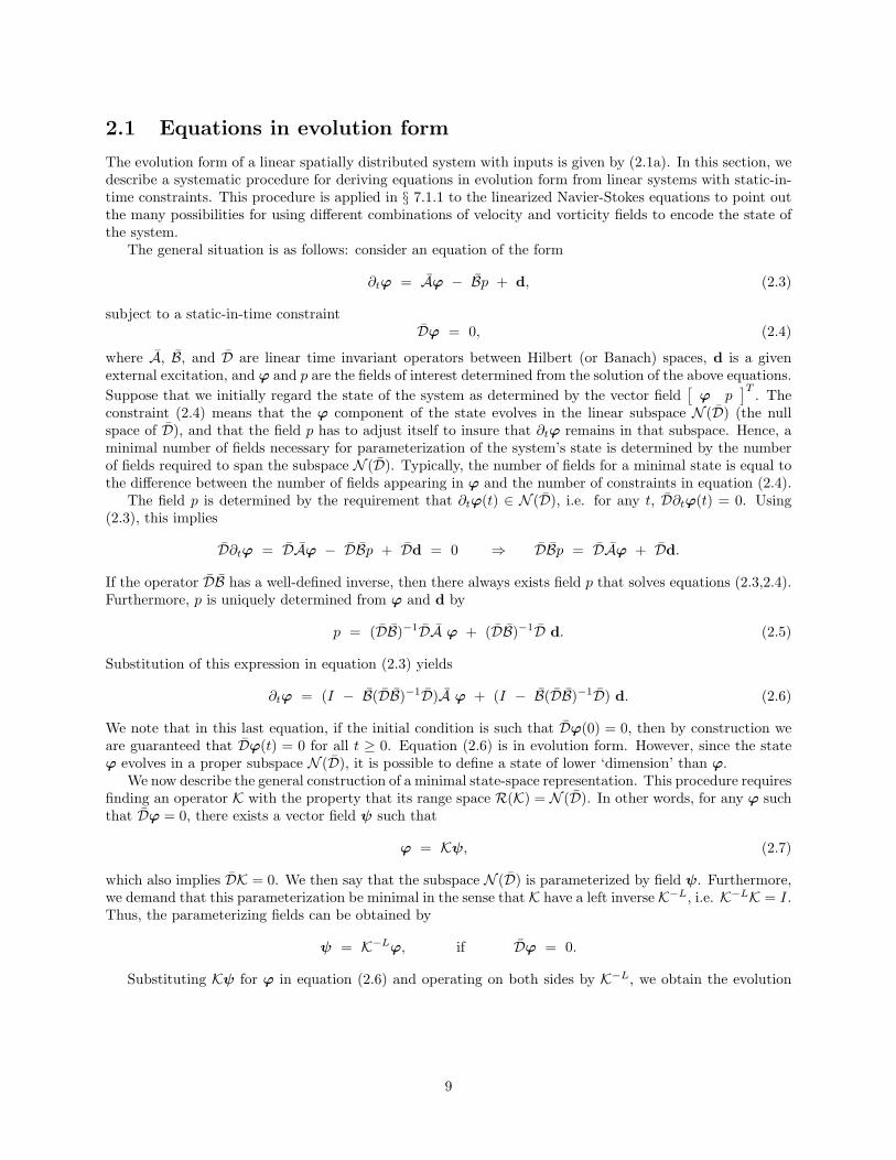
The evolution form of a linear spatially distributed system with inputs is given by (2.1a). In this section, wedescribe a systematic procedure for deriving equations in evolution form from linear systems with static-in-time constraints. This procedure is applied in § 7.1.1 to the linearized Navier-Stokes equations to point outthe many possibilities for using different combinations of velocity and vorticity fields to encode the state ofthe system.
The general situation is as follows: consider an equation of the form
∂tϕ = Aϕ − Bp + d, (2.3)
subject to a static-in-time constraintDϕ = 0, (2.4)
where A, B, and D are linear time invariant operators between Hilbert (or Banach) spaces, d is a givenexternal excitation, and ϕ and p are the fields of interest determined from the solution of the above equations.Suppose that we initially regard the state of the system as determined by the vector field
[ϕ p
]T . Theconstraint (2.4) means that the ϕ component of the state evolves in the linear subspace N (D) (the nullspace of D), and that the field p has to adjust itself to insure that ∂tϕ remains in that subspace. Hence, aminimal number of fields necessary for parameterization of the system’s state is determined by the numberof fields required to span the subspace N (D). Typically, the number of fields for a minimal state is equal tothe difference between the number of fields appearing in ϕ and the number of constraints in equation (2.4).
The field p is determined by the requirement that ∂tϕ(t) ∈ N (D), i.e. for any t, D∂tϕ(t) = 0. Using(2.3), this implies
D∂tϕ = DAϕ − DBp + Dd = 0 ⇒ DBp = DAϕ + Dd.
If the operator DB has a well-defined inverse, then there always exists field p that solves equations (2.3,2.4).Furthermore, p is uniquely determined from ϕ and d by
p = (DB)−1DA ϕ + (DB)−1D d. (2.5)
Substitution of this expression in equation (2.3) yields
∂tϕ = (I − B(DB)−1D)A ϕ + (I − B(DB)−1D) d. (2.6)
We note that in this last equation, if the initial condition is such that Dϕ(0) = 0, then by construction weare guaranteed that Dϕ(t) = 0 for all t ≥ 0. Equation (2.6) is in evolution form. However, since the stateϕ evolves in a proper subspace N (D), it is possible to define a state of lower ‘dimension’ than ϕ.
We now describe the general construction of a minimal state-space representation. This procedure requiresfinding an operator K with the property that its range space R(K) = N (D). In other words, for any ϕ suchthat Dϕ = 0, there exists a vector field ψ such that
ϕ = Kψ, (2.7)
which also implies DK = 0. We then say that the subspace N (D) is parameterized by field ψ. Furthermore,we demand that this parameterization be minimal in the sense that K have a left inverse K−L, i.e. K−LK = I.Thus, the parameterizing fields can be obtained by
ψ = K−Lϕ, if Dϕ = 0.
Substituting Kψ for ϕ in equation (2.6) and operating on both sides by K−L, we obtain the evolution
9

equation for ψ as
∂tψ = K−L(A − B(DB)−1DA)K ψ + K−L(I − B(DB)−1D) d=: A ψ + B d. (2.8)
Note that if this equation is solved forward in time, for any t ≥ 0, the original fields ϕ(t) and p(t) can befound from ψ(t) by solving equations (2.7) and (2.5). These equations involve only time-invariant operators.
Now, the construction of a K that has a left inverse, and is such that DK = 0, is not always obvious.However, a simple scheme can be devised by expressing these requirements in a ‘block operator’ decompositionas follows: [
DK−L
]K =
[0I
].
In the typical case that D has a right inverse D−R, these requirements are equivalent to[D
K−L
] [D−R K
]=
[I 00 I
].
Thus given D, if one can find an operator K−L such that the operator[
DK−L
]is invertible, then its inverse
can be partitioned into[D−R K
], and both K and K−L are obtained.
2.2 Dynamical systems with input and system uncertainty
In this section, we discuss the main features of the input-output analysis of spatially distributed lineardynamical systems. The results presented here have a fairly general character and can be applied to studythe input-output properties of
∂tψ(y, t, κ) = [A(κ)ψ(t, κ)](y) + [B(κ)d(t, κ)](y), (2.9a)φ(y, t, κ) = [C(κ)ψ(t, κ)](y), (2.9b)
where κ := [κ1 · · · κd ]∗ represents the vector of frequencies corresponding to the spatial coordinates ξ :=[ ξ1 · · · ξd ]∗ that belong to a certain group G [6]. On the other hand, y := [ y1 · · · yq ]∗ denotes the additionalspatial coordinates varying in set P without any group structure (that is, the spatial coordinates in which theunderlying operators are not translation invariant). We note that system (2.9) represents the transformedversion of
∂tψ(y, t, ξ) = [Aψ(t)](y, ξ) + [Bd(t)](y, ξ), (2.10a)φ(y, t, ξ) = [Cψ(t)](y, ξ), (2.10b)
obtained by the application of the Fourier transform in the spatially invariant directions. For notationalconvenience, we use the same notation to denote the field ψ(y, t, ξ) and its spatial Fourier transform ψ(y, t, κ).The distinction between the two should be clear from the context.
For example, a two-dimensional diffusion equation defined on the spatial domain R × [−1, 1]
∂tφ(y, t, x) = ∂xxφ(y, t, x) + ∂yyφ(y, t, x) + d(y, t, x),φ(±1, t, x) = 0, t ≥ 0, x ∈ R, y ∈ [−1, 1],
is translation invariant in the x direction, but it is not translation invariant in the y direction. The Fourierrepresentation of this system is given by (2.9) with A(κ) := ∂yy − κ2, B(κ) := I, C(κ) := I, κ ∈ R.The underlying state-space is a Hilbert space of square integrable functions L2[−1, 1], and the domain ofoperator A(κ) for any given κ is readily determined from the Dirichlet boundary conditions on φ (see, forexample, [2]).
Our presentation is organized as follows: in § 2.2.1, we introduce notions of spatio-temporal impulse and
10

frequency responses, and make some remarks about their utility in understanding behavior of linear systems.In § 2.2.2, we discuss different quantities that can be determined based on impulse and frequency responses,and define the notion of input-output system norms. In § 2.2.6, we illustrate that the problem of robuststability can be recast into the input-output framework and addressed using input-output tools.
2.2.1 Spatio-temporal impulse and frequency responses
We introduce the notion of the spatio-temporal frequency response as follows: let the input to (2.10) be afield that is harmonic in the t and ξ variables, that is of the form
d(y, t, ξ) = d(y)ei(κ·ξ + ωt),
where d(y) is some function of y, and κ · ξ := κT ξ. Assuming stability of the generator A, it can then beshown that the output is also harmonic in the same variables and is determined by
φ(y, t, ξ) = [H(ω, κ) d](y) ei(κ·ξ + ωt), (2.11)
where the operator H(ω, κ) is given by
H(ω, κ) = C(κ)(iωI −A(κ))−1B(κ). (2.12)
There are two possible interpretations of this. If this harmonic input is assumed to act over the time interval−∞ < t < ∞, then initial states do not play a role, and the output is precisely given by (2.11). If on theother hand the harmonic input is assumed to act over 0 ≤ t < ∞ with zero initial state (ψ(y, 0, ξ) = 0),then the output limits to (2.11) as transients asymptotically die out (due to stability) in the ‘steady-state’(that is, as t→ ∞).
Note that for each (ω, κ), H(ω, κ) is an operator in y. The operator-valued function H(ω, κ) in (2.12) iscalled the spatio-temporal frequency response of system (2.9). It is a function of temporal frequency ω andvector of spatial frequencies κ. Another interpretation of this function is that it maps the Fourier transformof the input to the Fourier transform of the output, that is
φ(y, ω, κ) = [H(ω, κ)d(ω, κ)] (y)
=∫
P
[H(ω, κ)] (y, η)d(η, ω, κ) dη,(2.13)
where by an abuse of notation we use the symbol [H(ω, κ)] (y, η) to denote the kernel function representingthe operator H(ω, κ).
On the other hand, the spatio-temporal impulse response of system (2.9) is determined by
H(t, κ) = C(κ)eA(κ)tB(κ), (2.14)
where eA(κ)t denotes the symbol for the operator semigroup generated by A(κ) [2]. Clearly, (2.14) representsan inverse temporal Fourier transform of (2.12). The terminology for the spatio-temporal impulse responseis due the fact that the kernel representation [H(t, κ)] (y, y0) of operator H(t, κ) represents the solution ofsystem (2.9) to a spatio-temporal impulsive input function δ(y − y0, t). The response to any other forcingfield d(y, t, κ) is then given by
φ(y, t, κ) =∫
P
∫ ∞
0
[H(t− τ, κ)] (y, η)d(η, τ, κ) dτ dη. (2.15)
The response in the physical space φ(y, t, ξ) can be obtained by applying the inverse spatial Fourier transformon (2.15), which results into
φ(y, t, ξ) =∫
G
∫P
∫ ∞
0
H(y, η, t− τ, ξ − ζ)d(η, τ, ζ) dτ dη dζ.
11

Clearly, function H(y, y0, t, ξ) represents the solution of system (2.10) to d(y, t, ξ) := δ(y − y0, t, ξ). Thus,the response to any forcing function in the physical space can be obtained as the superposition of a spatiallyand temporally shifted family of impulse responses.
To recap: given a particular spatio-temporal frequency response, there is a unique corresponding spatio-temporal impulse response that can be derived from it. Therefore, the frequency and impulse responsescontain the same information about the system’s dynamics. However, features of these dynamics are moreeasily seen in one or the other response.
2.2.2 Input-output system gains
The frequency response (2.12) contains a large amount of information about the dynamical behavior ofsystem (2.9). It is not always straightforward to visualize it since it is a function of temporal and spatialfrequency variables, and is also operator valued (or matrix valued after a suitable discretization in y). Here,we will mainly be interested in the behavior of the response as a function of the spatial frequencies. Therefore,we will need to somehow aggregate the effects of dynamics in t and y. This can be done in a variety of ways.We choose here to use the so-called H2 and H∞ system norms [7]. These are input-output norms of dynamicalsystems of the type (2.9), and they quantify the ‘amplification’ or ‘gain’ of a system, or in other words, therelative size of the output to the input. We note that there is no general relationship between the H2 andH∞ norms.
• The H2 norm is defined by
[‖H‖2
2
](κ) :=
12π
∫ ∞
−∞||H(ω, κ)||2HS dω =
∫ ∞
0
||H(t, κ)||2HS dt, (2.16)
where ‖ · ‖HS is the Hilbert-Schmidt norm of an operator defined by
‖H‖2HS := trace(HH∗) =
∞∑n=1
σ2n(H). (2.17)
The n-th singular value of operator H is denoted by σn(H). In the case when H is a matrix, this isprecisely the Frobenius norm.
• The H∞ norm is defined by[‖H‖∞] (κ) := sup
ωσmax(H(ω, κ)), (2.18)
where σmax is the maximum singular value.
These norms have interesting physical interpretations. We can regard H in (2.13) as representing the‘amplification’ or ‘gain’ from d to φ at given frequencies. The quantity (2.18) represents a maximization ofthis gain over input temporal frequencies and spatial shapes (by this we mean the variation of the input asa function of y). The former is obtained by the maximization over ω and the latter by taking a maximumsingular value. Thus, we can interpret the H∞ norm as the worst case amplification of inputs. Furthermore,we can find frequencies ω (the frequency at which supω is achieved) and κ, and input shape d(y) (namelythe right singular function corresponding to the maximum singular value) such that with input
d(y, t, ξ) = d(y)ei(κ·ξ + ωt),
the output φ has this worst case amplification, that is∫P
∫ ∞
0
φ∗(y, t, κ)φ(y, t, κ) dy dt = supκ
[‖H‖2
∞](κ).
On the other hand, the H2 norm has a stochastic interpretation: it quantifies the variance (energy)amplification of harmonic (in ξ) stochastic (in y and t) disturbances at any given κ. In the fluid mechanics
12

literature the H2 norm is also referred to as the ensemble average energy density of the statistical steady-state [8]. More generally, the frequency response operator captures the mapping of second order statisticsfrom the input to the output random fields. Let the input d be a zero-mean homogenous (in ξ and t) whiterandom field, i.e. one whose auto-correlation is
E d(y1, t1, ξ1)d∗(y2, t2, ξ2) = Iδ(y1 − y2, t1 − t2, ξ1 − ξ2),
where I is the identity matrix. The output random field will be stationary in ξ and t (but not in y), andwill have correlations determined by system’s dynamics. We define the auto-correlation function of φ afteraveraging in y by
Rφ(t, ξ) :=∫
P
∫P
E φ(y1, τ + t, ζ + ξ) φ∗(y2, τ, ζ) dy1 dy2.
Note that Rφ contains all the two-point correlation functions in ξ and t. Let Wφ be the Power SpectralDensity (PSD) function of φ obtained by a Fourier transform of Rφ. It is then a standard fact [9] that thePSD is given from system’s frequency response by
Wφ(ω, κ) := trace (H(ω, κ)H∗(ω, κ)) = ||H(ω, κ)||2HS .
Comparing this last expression with (2.16), we see that the H2 norm at each κ captures the total PSD atthis vector of spatial frequencies after integrating in temporal frequency.
We point out that for computing the H2 norm, the expression (2.16) can be determined without actuallyintegrating in ω. It is a standard fact from linear systems theory [7] that this quantity can be computedusing the solutions of the operator Lyapunov equations
A(κ)X∞(κ) + X∞(κ)A∗(κ) = −B(κ)B∗(κ),
A∗(κ)Y∞(κ) + Y∞(κ)A(κ) = −C∗(κ)C(κ),
where A∗, B∗, and C∗ respectively represent adjoints of operators A, B, and C. The H2 norm is thencomputed from either of the following two expressions[
‖H‖22
](κ) = trace (X∞(κ)C∗(κ)C(κ)) = trace (Y∞(κ)B(κ)B∗(κ)).
In the controls literature, operators X∞(κ) and Y∞(κ) are respectively referred to as the controllability andobservability Gramians [7].
The Hilbert-Schmidt norm of the impulse response operator can be also integrated over the finite timeinterval to yield: [
‖H‖22
](t, κ) :=
∫ t
0
‖H(τ, κ)‖2HS dτ .
The resulting measure of input-output amplification can be determined as[‖H‖2
2
](t, κ) = trace (Xt(κ)C∗(κ)C(κ)) = trace (Yt(κ)B(κ)B∗(κ)),
where operators Xt(κ) and Yt(κ) represent solutions of the following two differential Lyapunov equations
dXt(κ)dt
= A(κ)Xt(κ) + Xt(κ)A∗(κ) + B(κ)B∗(κ),
dYt(κ)dt
= A∗(κ)Yt(κ) + Yt(κ)A(κ) + C∗(κ)C(κ),(2.19)
13

with the initial conditions X0(κ) = 0 and Y0(κ) = 0, for every κ. For stable systems, these two operatorscan be determined based on
Xt(κ) = X∞(κ) − eA(κ)t X∞(κ) eA∗(κ)t,
Yt(κ) = Y∞(κ) − eA∗(κ)t Y∞(κ) eA(κ)t.
(2.20)
It is a standard fact from control theory [7, 10] that both H∞ and H2 norms are finite for stable causaldynamical systems. However, for unstable systems these measures of input-output amplification can becomeinfinitely large. Because of this, it is desirable to develop computationally efficient tools for determinationof the finite-horizon input-output gains for spatially distributed systems with unstable dynamics. In § 2.2.3,we define these gains and argue that their analysis represents a non-trivial mathematical exercise. In § 2.2.4,we propose an intuitively equivalent measure of input-output amplification by introducing the ‘exponentialdiscounting’ in signals appearing in (2.9).
2.2.3 Finite horizon input-output gains
In this subsection, we define the notion of finite horizon input-output system gains for system (2.9). Inparticular, we want to analyze the induced finite horizon 2 norm, that is, the induced norm of the so-called‘state space compression operator’ [11]. The definition of this norm in the temporal domain is given by
[‖HT ‖∞] (κ) = sup[‖dT ‖2](κ) ≤ 1
[‖φT ‖2](κ)[‖dT ‖2](κ)
, (2.21)
where
[‖dT ‖22](κ) :=
∫ T
0
[‖d‖22](κ, t) dt :=
∫ T
0
∫P
d∗(y, t, κ)d(y, t, κ) dy dt.
Clearly, the measure of input-output amplification defined by (2.21) represents a finite horizon equivalent ofthe previously defined H∞ norm. This quantity assumes finite values even for unstable systems, which isan appealing property. However, the computation of (2.21) is a non-trivial mathematical exercise (see, forexample, [11]).
Also, for unstable systems we can study [‖H‖2] (t, κ). We note that for system (2.9) with unstable dynam-ics Xt and Yt cannot be computed using (2.20) since both X∞ and Y∞ diverge in this case. Notwithstanding,[‖H‖2] (t, κ) can be determined by performing the direct numerical integration of the finite dimensional equiv-alent of either of the two equations in (2.19). This would typically require solving a very large number ofODEs which is computationally inefficient. For this reason, in § 2.2.4, we show how these finite horizoninput-output gains can be approximately determined by considering the ‘exponentially discounted’ versionsof signals in (2.9).
2.2.4 Exponentially discounted input-output gains
In this subsection, we define the input-output gains for unstable spatially distributed systems with ‘expo-nentially discounted’ inputs and outputs, that is dα := e−αtd, φα := e−αtφ, with α > 0. Transformationof this form renders (2.9) into
∂tψα(y, t, κ) = [Aα(κ)ψα(t, κ)](y) + [B(κ)dα(t, κ)](y), (2.22a)φα(y, t, κ) = [C(κ)ψα(t, κ)](y), (2.22b)
where ψα := e−αtψ is the exponentially weighted state of (2.9). Input and output operators B and C havethe same meaning as in (2.9), whereas the generator of (2.22) is obtained by shifting the generator of (2.9) bythe amount proportional to the exponential discounting, i.e. Aα(κ) := A(κ) − αI. The frequency domain
14

description of (2.22) is clearly given by
φα(y, ω, κ) = [Hα(ω, κ)dα(ω, κ)] (y)
=[C(κ)(iωI − Aα(κ))−1B(κ)dα(ω, κ)
](y)
=[C(κ)((iω + α)I − A(κ))−1B(κ)dα(ω, κ)
](y).
If parameter α is chosen so that α > supκ λmaxA(κ), than Aα(κ) represents an exponentially stableoperator for any given κ. Therefore, the net effect of exponential discounting in this case is stabilizationof (2.9) which implies that the H∞ and H2 norms of system (2.22) can be computed using the procedureoutlined in § 2.2.2. In particular, the following interpretation can be given to the H∞ norm of (2.22) in thetime domain
[‖Hα‖∞] (κ) = sup[‖dα‖2](κ) ≤ 1
[‖φα‖2](κ)[‖dα‖2](κ)
,
where[‖dα‖2
2](κ) :=∫ ∞
0
∫P
d∗α(y, t, κ)dα(y, t, κ) dy dt
=∫ ∞
0
∫P
e−2αtd∗(y, t, κ)d(y, t, κ) dy dt
=∫ ∞
0
e−2αt[‖d‖22](t, κ) dt.
On the other hand, for a given κ and t > 0, the ‘finite horizon H2 norm’ of system (2.9) at time t can bedetermined by the H2 norm of system (2.22), provided that the design parameter α is appropriately selected.This is because [‖H‖2] (t, κ) represents a monotonically increasing function of time which is equal to zeroat t = 0, and [‖Hα‖2] (κ) is a finite number for any given κ. Unfortunately, in general, it is very difficultto establish the exact correspondence between [‖H‖2] (t, κ) and [‖Hα‖2] (κ). In other words, it is very hardto determine pair (t, α) at which [‖H‖2] (t, κ) = [‖Hα‖2] (κ). However, some intuition can be gained byconsidering the following scalar example
ψ = aψ + d
φ = ψ
, a > 0, (2.23)
with its ‘exponentially discounted’ equivalent of the form
ψα = (a − α)ψα + dα
φα = ψα
, α > a. (2.24)
The ‘finite horizon H2 norm’ of system (2.23) and the H2 norm of system (2.24) are respectively given by
[‖H‖2
2
](t) =
12a
(e2at − 1),
‖Hα‖22 =
12a(α − a)
,
which implies that, for a chosen α > a, [‖H‖2] (t) = ‖Hα‖2 at
t =12a
lnα
α − a.
Equivalently, for a given t > 0, these two quantities are equal if α satisfies
α =ae2at
e2at − 1.
15

Therefore, both the location of the unstable pole and the desired time interval determine the value ofparameter α for which the H2 norm of system (2.24) determines the ‘finite horizon H2 norm’ of system (2.23).Furthermore, the closer α to a and the smaller a, the larger time at which [‖H‖2] (t) = ‖Hα‖2.
2.2.5 Input-output directions
As mentioned above, at fixed frequencies (ω, κ), H(ω, κ) represents an operator in y. Since this operator iscompact [2], we can study its properties using the singular value (Schmidt) decomposition
[H(ω, κ)d(ω, κ)](y) =∞∑m=1
σm(ω, κ) 〈d, ιm〉om(y, ω, κ), (2.25)
where σm ≥ 0m∈N are the singular values of H arranged in descending order, and ιmm∈N, omm∈N
are respectively the right and the left singular functions, that is
[H∗(ω, κ)H(ω, κ) ιm(ω, κ)](y) = σ2m(ω, κ)ιm(y, ω, κ),
[H(ω, κ)H∗(ω, κ)om(ω, κ)](y) = σ2m(ω, κ)om(y, ω, κ).
By substituting d(y, ω, κ) := ιn(y, ω, κ), n ∈ N, in (2.25) we obtain
[H(ω, κ)ιn(ω, κ)](y) = σn(ω, κ)on(y, ω, κ).
This relationship illustrates that an input in the direction ιn(y, ω, κ) produces the output in the directionon(y, ω, κ). For this reason, functions ιn(y, ω, κ) and on(y, ω, κ) are respectively referred to as the input andoutput directions. On the other hand, σn(ω, κ) represents the input-output gain when the system is excitedin the direction ιn(y, ω, κ). Since the singular values of H(ω, κ) are arranged in descending order, the largestgain in any input direction is determined by σ1(ω, κ): the maximal singular value of the frequency responseoperator. The corresponding vectors ι1(y, ω, κ) and o1(y, ω, κ) respectively represent the most amplifiedinput direction and the output direction in which the inputs are most efficient. These directions are referredto as the worst-case input and output directions at any given (ω, κ). The worst-case input and outputdirections over all frequencies are the ones that correspond to supκ,ω σmax(H(ω, κ)) =: supκ[‖H‖∞](κ).Clearly, the notion of worst-case directions is well defined only for stable systems, since otherwise, thereexist input directions that lead to unbounded amplification by the system’s dynamics.
2.2.6 Robustness analysis versus input-output analysis
In this subsection, we illustrate that the problem of robust stability can be addressed using input-outputtools. In particular, we apply a small gain theorem to show that the robust stability analysis is equivalent tothe input-output analysis for certain part of the system. In other words, we utilize input-output approachto cast the problem under study into a fairly general framework which allows for consideration of seeminglydifferent issues.
Consider a system of the form∂tψ = Aψ, (2.26)
where, in general, A is an operator. For example, the unforced evolution model (2.1a) can be representedby (2.26). Let us assume that operator A generates the strongly continuous (Co) semigroup eAt on theunderlying Hilbert space H. To characterize the exponential stability2 of eAt we need to introduce the notionof resolvent of the operator A. This quantity is the operator valued function defined on the resolvent setρ(A),
ρ(A) :=s ∈ C; (sI − A)−1 exists & ‖(sI − A)−1‖ <∞ on H
,
byR : ρ(A) → B(H,H), R(A) := (sI − A)−1,
2Co semigroup eAt is exponentially stable if and only if ‖eAt‖ ≤ M e−αt, t ≥ 0, for some M, α > 0.
16

where B(H,H) denotes the space of all bounded linear operators from H to H.It is a standard fact that eAt is exponentially stable [2] if and only if the R(A) satisfies the following
condition:sup
Re(s)>0
‖R(A)‖ < ∞.
Clearly, if an additional term is added to the right-hand side of (2.26),
∂tψ = Aψ + d, (2.27)
then the resolvent can be determined as the transfer function from the input d to the state ψ. Therefore,using the maximum modulus principle, it follows that the condition for the exponential stability of eAt isprecisely given in terms of the H∞ norm of system (2.27), with ψ being considered as the output. This isyet another interesting interpretation of the H∞ norm.
We note that, for all systems that we consider in this dissertation, the exponential stability of eAt canbe also characterized by the spectrum of the operator A. In this case, the exponential stability of eAt isequivalent to the requirement that the spectrum of A belongs to the open left-half of the complex plane.The spectrum of A is a closed subset of the complex plane defined by
σ(A) := C \ ρ(A) = s ∈ C, (sI −A) is not ‘boundedly invertible’ .
A certain operator is not ‘boundedly invertible’ if it is either non-invertible (not one-to-one), or if its inverserepresents an unbounded operator.
Also, we are interested in a problem of robust stability of eAt, which can be formulated as a stabilityproblem for a system
∂tψ = (A + Γ)ψ, (2.28)
where Γ is a bounded operator with ||Γ||∞ ≤ ε. Consideration of this problem can be justified by a lackof complete knowledge of the elements of A. Arguably, (2.26) is just a model of a physical system and, nomatter how carefully the modeling has been performed, there will always be some discrepancies betweenthe two. Modeling uncertainties can be rigorously accounted for by introducing operator Γ. This type ofuncertainty is usually referred to as unstructured uncertainty, and it can be seen as ubiquitous errors whichcan be associated with all models [7]. However, this representation of uncertainty can be too conservativesince some additional information about the structure of uncertainty is usually available. A more refinedmodel can be obtained by considering a lower rank uncertainty problem
∂tψ = (A + BΓC)ψ, (2.29)
where B and C are known operators of certain structure. The problem formulated in this fashion is moregeneral than problem (2.28) since the latter can be recovered from the former by the appropriate choice ofB and C (B = I, C = I). Because of this, we consider system (2.29) and study its stability properties.
Robust stability of (2.26) is guaranteed if and only if the resolvent of A + BΓC satisfies
supRe(s)>0
‖R(A + BΓC)‖ < ∞, ∀ ||Γ||∞ ≤ ε. (2.30)
For the systems under study in this dissertation, condition (2.30) is satisfied if the spectrum of A + BΓCbelongs to the open left-half of the complex plane for all ||Γ||∞ ≤ ε. This requirement can be expressed interms of the so-called pseudo-spectra [12–14], which is defined as
σε(A) := s ∈ C, ∃ ||Γ||∞ ≤ ε s.t. (sI − (A + BΓC)) is not ‘boundedly invertible’ . (2.31)
The original definition of pseudo-spectra is given for B = I, C = I and, thus, expression (2.31) is a slightgeneralization of this concept.
17

d∂tψ = Aψ + Bd
ψC
φ
Γ
Figure 2.2: Block diagram of system (2.29) in a form suitable for the application of small gain theorem.
We now illustrate that system (2.29) can be represented by a feedback system of the form
∂tψ = Aψ + Bd,φ = Cψ, (2.32)
by the appropriate choice of input d. Namely, by defining d as d := Γφ, we can readily recover (2.29)from (2.32). This representation is illustrated by a symbolic block diagram shown in Figure 2.2, where theknown part of the system is separated from the uncertain part of the system. The system represented inthis way is suitable for application of the small gain theorem. This theorem provides a test for stability of anominally stable system with the operator-valued transfer function H(s) := C(sI − A)−1B in the presenceof unstructured uncertainty Γ.
Theorem 1 The system shown in Figure 2.2 is internally stable for all ||Γ||∞ ≤ ε if and only if ||H||∞ <1ε.
Hence, it has been established that the robust stability analysis is mathematically equivalent to the input-output analysis for a certain part of the system. Therefore, without loss of generality, input-output analysiscan be performed with keeping in mind that, by doing so, the robust stability analysis can be captured aswell.
Finally, we note that the pseudo-spectrum can be determined by computing the level sets of the functionσmaxC(sI − A)−1B. In other words,
σε(A) =s ∈ C, σmaxC(sI − A)−1B ≥ 1
ε
.
Thus, it has been illustrated that the input-output analysis has a very general character and that it can, inparticular, be used for studying the problem of robust stability of dynamical systems.
18

Bibliography
[1] E. W. Kamen, “Stabilization of linear spatially-distributed continuous-time and discrete-time systems,”in Multidimensional Systems Theory, N. K. Bose, Ed. Hingham, MA: Kluwer, 1985.
[2] R. F. Curtain and H. J. Zwart, An Introduction to Infinite-Dimensional Linear Systems Theory. NewYork: Springer-Verlag, 1995.
[3] J. L. Lions, Optimal Control of Systems Governed by Partial Differential Equations. New York:Springer-Verlag, 1971.
[4] S. P. Banks, State-Space and frequency-domain methods in the control of distributed parameter systems.London, UK: Peter Peregrinus Ltd., 1983.
[5] Z. Luo, B.Z.Guo, and O.Morgul, Stability and Stabilization of Infinite Dimensional Systems with Ap-plications. London: Springer-Verlag, 1999.
[6] B. Bamieh, F. Paganini, and M. A. Dahleh, “Distributed control of spatially invariant systems,” IEEETransactions on Automatic Control, vol. 47, no. 7, pp. 1091–1107, July 2002.
[7] K. Zhou, J. C. Doyle, and K. Glover, Robust and Optimal Control. Prentice Hall, 1996.
[8] B. F. Farrell and P. J. Ioannou, “Stochastic forcing of the linearized Navier-Stokes equations,” Physicsof Fluids A, vol. 5, no. 11, pp. 2600–2609, 1993.
[9] E. VanMarcke, Random Fields: Analysis and Synthesis. MIT Press, 1983.
[10] G. E. Dullerud and F. Paganini, A course in robust control theory: a convex approach. New York:Springer-Verlag, 2000.
[11] G. E. Dullerud, “Computing the L2-induced norm of a compression operator,” Systems and ControlLetters, vol. 37, pp. 87–91, 1999.
[12] L. N. Trefethen, A. E. Trefethen, S. C. Reddy, and T. A. Driscoll, “Hydrodynamic stability withouteigenvalues,” Science, vol. 261, pp. 578–584, 1993.
[13] S. C. Reddy and D. S. Henningson, “Energy growth in viscous channel flows,” J. Fluid Mech., vol. 252,pp. 209–238, 1993.
[14] L. N. Trefethen, “Pseudospectra of linear operators,” SIAM Rev., vol. 39, no. 3, pp. 383–406, 1997.
19

Chapter 3
Exact determination of frequencyresponses for a class of spatiallydistributed systems
In this chapter, we study frequency responses of the distributed systems in which a spatial independentvariable belongs to a finite interval. Computation of frequency responses for this class of systems is usuallydone numerically by resorting to finite dimensional approximations of the underlying operators. We show thatthe spatial discretization can be circumvented and that frequency responses can be determined explicitlywhenever the underlying operators can be represented by forced Two Point Boundary Value State-spaceRealizations (TPBVSR) which are well posed.
Our results build on the work presented in [1], where a formula for the trace of a class of differentialoperators defined by forced TPBVSR with constant coefficients was derived. This formula was used forcomputation of the H2 norm for a class of infinite dimensional systems in which the dynamical generatorsare normal (or self-adjoint). Here we study the spatio-temporal frequency responses of spatially distributedsystems with, in general, non-normal dynamical generators and non-constant coefficients in a spatially inde-pendent variable. The fields of interest are assumed to satisfy the boundary conditions expressed in termsof a general linear homogeneous constraint. Our main result is an explicit formula for the Hilbert–Schmidtnorm (that is, the power spectral density) of the frequency response operator. This formula involves onlyfinite dimensional computations with matrices whose dimension is at most four times larger than the orderof the underlying differential operator. In this way an exact reduction of an infinite dimensional problem toa finite dimensional problem is accomplished.
Our presentation is organized as follows: in § 3.1, we formulate the problem and briefly review the notionof frequency responses for spatially distributed systems. In § 3.2, we show how the frequency responses canbe determined explicitly without resorting to the finite dimensional approximations. In § 3.3, we provide anexample to illustrate the application of the developed procedure. An additional example, that shows howthe Hilbert–Schmidt norms can be obtained explicitly for a system that describes the dynamics of velocityfluctuations in channel fluid flows, is given in § 9.5. We conclude by summarizing major contributions in§ 3.4.
3.1 Preliminaries
We consider spatially distributed systems of the form
∂tψ(y, t) = [Aψ(t)](y) + [Bd(t)](y), (3.1a)
φ(y, t) = [Cψ(t)](y), (3.1b)
20

where A, B, and C are linear operators, d is a forcing term, and ψ and φ are fields of interest determinedby the solution of the above equation. The spatial independent variable y is assumed to belong to a finiteinterval [a, b], with a ∈ R, b ∈ R, and a < b. We remark that (3.1) can be also used to describe multi-dimensional distributed systems that are spatially invariant in the remaining spatial directions [2]. In thiscase, the application of the spatial Fourier transform in these directions renders differential/integral operatorsinto multiplication operators which results in a one-dimensional system parameterized by a vector of spatialfrequencies κ
∂tψ(y, t, κ) = [A(κ)ψ(t, κ)](y) + [B(κ)d(t, κ)](y), (3.2a)
φ(y, t, κ) = [C(κ)ψ(t, κ)](y). (3.2b)
Our objective is to investigate dynamical properties of system (3.1) or system (3.2) by computing theirfrequency responses. The frequency response of (3.1) is determined by [3]
H(ω) := C(iωI − A)−1B,
where ω denotes the temporal frequency. Similarly, the spatio-temporal frequency response of system (3.2)is given by
H(ω, κ) := C(κ)(iωI − A(κ))−1B(κ).
In the remainder of this chapter we discuss the latter notion, because it is more general.We remark that for any given pair (ω, κ), H(ω, κ) represents an operator in y that maps d(y, ω, κ) into
φ(y, ω, κ) according toφ(y, ω, κ) = [H(ω, κ)d(ω, κ)] (y)
=∫ b
a
[H(ω, κ)] (y, η)d(η, ω, κ) dη,(3.3)
where by an abuse of notation we use the symbol [H(ω, κ)] (y, η) to denote the kernel function representingthe operator H(ω, κ). We assume that, for any given pair (ω, κ), [H(ω, κ)] (y, η) represents a continuousmatrix valued function on [a, b] × [a, b]. It is a standard fact that under these conditions H(ω, κ) is aHilbert–Schmidt operator [4]. Thus, we can determine the Hilbert–Schmidt norm of H(ω, κ) as
||H(ω, κ)||2HS := trace(H(ω, κ)H∗(ω, κ)) =∫ b
a
tr ([F(ω, κ)](y, y)) dy,
where [F(ω, κ)](y, ξ) denotes the kernel representation of the operator F(ω, κ) := H(ω, κ)H∗(ω, κ), whereastrace(·) and tr(·) respectively denote the traces of the argument operator and the argument matrix.
Computation of ||H(ω, κ)||HS is usually done numerically for any given pair (ω, κ), after finite dimensionalapproximations of the underlying operators are determined by the appropriate spatial discretization. In § 3.2,we show that the Hilbert–Schmidt norm of H(ω, κ) can be determined explicitly without resorting to thefinite dimensional approximations, whenever H(ω, κ) can be represented by a TPBVSR which is well posed.
3.2 Determination of frequency responses from state-space real-izations
In this section, instead of usual finite dimensional approximations of the underlying operators, we derive anexplicit formula for the Hilbert–Schmidt norm (i.e., the power spectral density) of the frequency responseoperator. This formula only involves finite dimensional computations with matrices whose dimension is atmost four times larger than the order of the underlying differential operators. Before presenting the mainresult in § 3.2.3, we discuss state-space realizations of H, H∗, and HH∗ in § 3.2.1, and show how the traceof a certain differential operator can be determined from its TPBVSR in § 3.2.2.
21

3.2.1 State-space realizations of H, H∗, and HH∗
We assume that the operator H(ω, κ) : d(ω, κ) → φ(ω, κ) in (3.3) can be represented by a well-posedTPBVSR of the following form1
H :
x′(y) = A0(y)x(y) + B0(y)d(y),
φ(y) = C0(y)x(y),
0 = N1x(a) + N2x(b), y ∈ [a, b],
(3.4)
where x′(y) := dx(y)/dy. The dependence on ω and κ is suppressed for notational convenience. Furthermore,for any given pair (ω, κ), A0(y), B0(y), and C0(y) are matrix valued functions (with, in general, non-constantcoefficients in y), defined on the interval [a, b], of respective dimensions n0 × n0, n0 × p, and m × n0. Theboundary value matrices N1 and N2 are constant and have dimension n0 × n0. These matrices have to besuch that
[N1 N2
]has a full row rank, to prevent a redundancy in boundary conditions. We remark
that TPBVSR (3.4) is well-posed (that it, has a unique solution for any input d(y)) if and only if [5]
det(N1 + N2Φ0(b, a)) = 0,
where Φ0(y, η) denotes the state transition matrix of A0(y).It can be shown that the adjoint of the operator H(ω, κ), H∗(ω, κ) : f(ω, κ) → d(ω, κ), can be represented
by a well-posed TPBVSR of the following form
H∗ :
z′(y) = −A∗0(y)z(y) − C∗
0 (y)f(y),
d(y) = B∗0(y)z(y),
0 = M1z(a) + M2z(b), y ∈ [a, b],
(3.5)
where A∗0, B
∗0 , and C∗
0 respectively represent the adjoints (complex-conjugate-transpose matrices) of A0, B0,and C0. On the other hand, the constant boundary value matrices M1 and M2 are determined by
[M1 M2
] [ N∗1
−N∗2
]= 0. (3.6)
We note that a variety of different M1 and M2 for which[M1 M2
]is a full row rank matrix can be chosen
to satisfy (3.6). For example, a Singular Value Decomposition of a full column rank matrix[
N∗1
−N∗2
]:
[N∗
1
−N∗2
]= USV ∗ =
[U1 U2
] [ S1
0
]V ∗ = U1S1V
∗, U1, U2 ∈ C2n0×n0 ,
can be used to select these two matrices as[M1 M2
]= U∗
2 .
Thus, a well-posed state-space realization of H(ω, κ)H∗(ω, κ) : f(ω, κ) → φ(ω, κ) can be obtained bycombining (3.4) and (3.5)
HH∗ :
q′(y) = A(y)q(y) + B(y)f(y),
φ(y) = C(y)q(y),
0 = L1q(a) + L2q(b), y ∈ [a, b],
(3.7)
1In § 3.3 and § 9.5, we illustrate, by means of two examples, how this can be done.
22

where
q(y) :=[x(y)z(y)
]∈ C
2n0 , L1 :=[N1 00 M1
], L2 :=
[N2 00 M2
],
A(y) :=
[A0(y) B0(y)B∗
0(y)
0 −A∗0(y)
], B(y) :=
[0
−C∗0 (y)
], C(y) :=
[C0(y) 0
].
In § 3.2.2, we show how trace(HH∗) can be determined from the TPBVSR of HH∗ (3.7).
3.2.2 Determination of traces from state-space realizations
We study a well-posed TPBVSR of the form
F :
q′(y) = A(y)q(y) + B(y)f(y),
φ(y) = C(y)q(y),
0 = L1q(a) + L2q(b), y ∈ [a, b],
(3.8)
with q(y) ∈ Cn, f(y) ∈ C
m, φ(y) ∈ Cm, and derive an explicit formula for the trace of operator F : f → φ.
This formula, as we will show, is expressed in terms of matrices A(y), B(y), C(y), L1, L2, and it onlyrequires computation of two state transition matrices: the state transition matrix of A(y), and the statetransition matrix of a matrix that depends on A(y), B(y), and C(y). The size of the latter matrix is 2n×2n.Our results generalize the results of [1], where the trace formula for operators with constant coefficients andless general boundary conditions was derived. Here we study the problem with non-constant coefficients iny. In addition to that, the boundary conditions are given as a general linear homogeneous constraint on q(y)at y = a, b.
We utilize the fact that the trace of an operator F : f → φ
φ(y) =∫ b
a
F(y, η)f(η) dη, (3.9)
with a continuous kernel F(y, η) is determined by
trace(F) =∫ b
a
tr (F(yo, yo)) dyo =∫ b
a
tr
(m∑k=1
F(yo, yo)ekeTk
)dyo,
where ek denotes the k-th unit vector in Rm. Clearly, each ‘column’ of the kernel can be obtained by
forcing (3.9) with an impulsive function (that is, if f(y) = δ(y − yo)ek then F(y, yo)ek = φ(y)). Thus, forany given yo ∈ [a, b], F(yo, yo)ek represents a response φ(y) evaluated at y = yo to input f(y) = δ(y− yo)ek.The effect of forcing (3.8) with f(y) = δ(y − yo)ek is given by
q′(y) = A(y)q(y) + B(y)δ(y − yo)ek ⇒
q′(y) = A(y)q(y),q(y+
o ) − q(y−o ) = B(yo)ek,
where q(y+o ) and q(y−o ) respectively represent the limits of q(y) as yo is approached from above and below
(see Figure 3.1). Hence,
q′(y) = A(y)q(y),q(y+
o ) − q(y−o ) = B(yo)ek,
⇒ Φ(yo, b)q(b) − Φ(yo, a)q(a) = B(yo)ek, (3.10)
where Φ(y, η) denotes the state transition matrix of A(y). By combining the boundary conditions from (3.9)
23
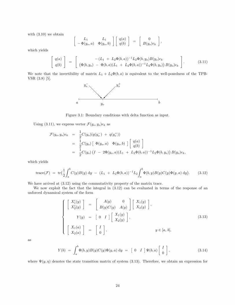
with (3.10) we obtain [L1 L1
−Φ(yo, a) Φ(yo, b)
] [q(a)q(b)
]=
[0
B(yo)ek
],
which yields [q(a)
q(b)
]=
[− (L1 + L2Φ(b, a))−1L2Φ(b, yo)B(yo)ek(
Φ(b, yo) − Φ(b, a)(L1 + L2Φ(b, a))−1L2Φ(b, yo))B(yo)ek
]. (3.11)
We note that the invertibility of matrix L1 + L2Φ(b, a) is equivalent to the well-posedness of the TPB-VSR (3.8) [5].
a byo
y+oy−o
Figure 3.1: Boundary conditions with delta function as input.
Using (3.11), we express vector F(yo, yo)ek as
F(yo, yo)ek =12C(yo)(q(y−o ) + q(y+
o ))
=12C(yo)
[Φ(yo, a) Φ(yo, b)
] [ q(a)q(b)
]=
12C(yo)
(I − 2Φ(yo, a)(L1 + L2Φ(b, a))−1L2Φ(b, yo)
)B(yo)ek,
which yields
trace(F) = tr(12
∫ b
a
C(y)B(y) dy − (L1 + L2Φ(b, a))−1L2
∫ b
a
Φ(b, y)B(y)C(y)Φ(y, a) dy). (3.12)
We have arrived at (3.12) using the commutativity property of the matrix trace.We now exploit the fact that the integral in (3.12) can be evaluated in terms of the response of an
unforced dynamical system of the form
[X ′
1(y)X ′
2(y)
]=
[A(y) 0
B(y)C(y) A(y)
] [X1(y)X2(y)
],
Y (y) =[
0 I] [ X1(y)
X2(y)
],
[X1(a)X2(a)
]=
[I
0
], y ∈ [a, b],
(3.13)
as
Y (b) =∫ b
a
Φ(b, y)B(y)C(y)Φ(y, a) dy =[
0 I]Ψ(b, a)
[I
0
], (3.14)
where Ψ(y, η) denotes the state transition matrix of system (3.13). Therefore, we obtain an expression for
24

trace(F) by combining (3.12) and (3.14)
trace(F) = tr(12
∫ b
a
C(y)B(y) dy − (L1 + L2Φ(b, a))−1L2
[0 I
]Ψ(b, a)
[I
0
] ). (3.15)
In particular, for systems with constant coefficients in y formula (3.15) simplifies to
trace(F) = tr(c
2CB − (L1 + L2ecA)−1L2
[0 I
]exp
c
[A 0BC A
][I
0
]), (3.16)
where c := b− a. Furthermore, for operators F with
A(y) := A, B(y) := e−α(y− a)B, C(y) := C,
formula (3.15) simplifies to
trace(F) =1 − e−αc
2αtr (CB) −
tr(
(L1 + L2ecA)−1L2
[0 I
]exp
c
[A − αI 0BC A
][I
0
]),
(3.17)
Clearly, in the limit as α → 0, expression on the right-hand side of (3.17) approaches the expression on theright-hand side of (3.16). Trace formulae (3.16) and (3.17) are used in Chapter 9 to explicitly determine theH2 norms of the linearized Navier-Stokes equations in channel flows.
In § 3.2.3, we combine the results of § 3.2.1 and § 3.2.2 to provide an explicit formula for the Hilbert–Schmidt norm of the frequency response operator.
3.2.3 Explicit formula for Hilbert–Schmidt norm
The main result of this chapter is summarized in the following theorem.
Theorem 2 The Hilbert–Schmidt norm of the frequency response operator H(ω, κ) : d(ω, κ) → φ(ω, κ),given by a well-posed TPBVSR (3.4), is determined by
||H(ω, κ)||2HS = − tr((L1 + L2Φ(b, a))−1L2
[0 I
]Ψ(b, a)
[I
0
] ), (3.18)
where
L1 :=[N1 00 M1
], L2 :=
[N2 00 M2
],
A(y) :=
[A0(y) B0(y)B∗
0(y)
0 −A∗0(y)
], B(y) :=
[0
−C∗0 (y)
], C(y) :=
[C0(y) 0
].
Matrices M1 and M2 are determined from the following Singular Value Decomposition[N∗
1
−N∗2
]= USV ∗ =
[U1 U2
] [ S1
0
]V ∗ = U1S1V
∗, U1, U2 ∈ C2n0×n0 ,
by [M1 M2
]= U∗
2 .
25

On the other hand, Φ(y, η) and Ψ(y, η) respectively denote the state transition matrices of A(y) and[A(y) 0
B(y)C(y) A(y)
].
For systems with constant coefficients in y formula (3.18) simplifies to
||H(ω, κ)||2HS = − tr(
(L1 + L2ecA)−1L2
[0 I
]exp
c
[A 0BC A
][I
0
]), (3.19)
where c := b− a.
Hence, we have converted a problem of evaluating the Hilbert–Schmidt norm of an infinite dimensionalobject to computations with finite matrices. For systems with non-constant coefficients in y, at any given(ω, κ), we need to solve a differential equation whose order is four times larger than the order of the originaldifferential operator to obtain the state transition matrix Ψ(b, a). On the other hand, for systems withconstant coefficients in y this computation amounts to determination of the corresponding matrix exponen-tial. Both computations can be easily performed using commercially available software such as matlab ormathematica.
In § 3.3 and § 9.5, we illustrate the application of this procedure and exactly determine the frequencyresponses of two systems: a one-dimensional diffusion equation, and a system that describes the dynamicsof velocity fluctuations in channel fluid flows.
3.3 Examples
In this section, we illustrate how the frequency responses of a one-dimensional diffusion equation can bedetermined explicitly using the previously described procedure. In § 9.5, we also employ Theorem 2 to de-termine the Hilbert–Schmidt norms of the streamwise constant linearized Navier-Stokes equations in channelflows.
3.3.1 A one-dimensional diffusion equation
We consider a one-dimensional diffusion equation on L2[−1, 1] with Dirichlet boundary conditions
∂tψ(y, t) = [∂yyψ(t)](y) + d(y, t),ψ(±1, t) = 0.
The application of the temporal Fourier transform yields
ψ(y, ω) = [(iωI − ∂yy)−1d(ω)](y) =: [H(ω)d(ω)](y).
Our objective is to compute the Hilbert–Schmidt norm of operator that maps d into ψ as a function oftemporal frequency ω. A particular TPBVSR of H(ω) is given by
H(ω) :
[x′1(y, ω)x′2(y, ω)
]=
[0 1iω 0
] [x1(y, ω)x2(y, ω)
]+
[0
−1
]d(y, ω),
ψ(y, ω) =[
1 0] [ x1(y, ω)
x2(y, ω)
],
0 =[
1 00 0
] [x1(−1, ω)x2(−1, ω)
]+
[0 01 0
] [x1(1, ω)x2(1, ω)
], y ∈ [−1, 1].
26

The application of procedure described in § 3.2.1 yields the realization of H(ω)H∗(ω) in the form of (3.7)with
A =
0 1 0 0iω 0 0 10 0 0 iω0 0 −1 0
, B =
00
−10
, C =
[1 0 0 0
],
L1 =
1 0 0 00 0 0 00 0 0 10 0 0 0
, L2 =
0 0 0 01 0 0 00 0 0 00 0 0 1
.
The application of (3.19), with the help of mathematica, yields
||H(ω)||2HS =1
2ω2
−1 +
√2ω(sinh(
√8ω) + sin(
√8ω))
cosh(√
8ω) − cos(√
8ω)
. (3.20)
It is noteworthy that ||H(ω)||2HS can be also obtained by doing a spectral decomposition of the operator∂yy. It is well known (see, for example [3]) that this operator with Dirichlet boundary conditions has thefollowing set of orthonormal eigenfunctions ϕnn∈N with corresponding eigenvalues γnn∈N
ϕn(y) := sin(nπ
2(y + 1)
), γn := − n2π2
4, n ∈ N.
It is easily shown that the eigenfunction expansion results into
||H(ω)||2HS =∑n∈N
1
ω2 +(nπ
2
)4 ,
which can be summed to obtain (3.20). However, for operators that do not have explicit expressions for theireigenvalues, it is much easier to compute the trace explicitly as we illustrate in § 9.5.
3.4 Summary
We develop a procedure for the explicit determination of the frequency responses for a class of spatiallydistributed systems. This procedure avoids the need for spatial discretization and provides an exact reductionof an infinite dimensional problem to a problem in which only matrices of finite dimensions are involved.The order of these matrices is at most four times larger than the order of the differential operator at hand.
We also illustrate application of this technique by providing two examples: a one-dimensional diffusionequation (see § 3.3.1), and a system obtained by linearization of the Navier-Stokes equations in channel flowsaround a given nominal velocity profile (see § 9.5).
27

Bibliography
[1] B. Bamieh and M. Dahleh, “Exact computation of traces and H2 norms for a class of infinite dimensionalproblems,” IEEE Transactions on Automatic Control, vol. 48, no. 4, pp. 646–649, April 2003.
[2] B. Bamieh, F. Paganini, and M. A. Dahleh, “Distributed control of spatially invariant systems,” IEEETransactions on Automatic Control, vol. 47, no. 7, pp. 1091–1107, July 2002.
[3] R. F. Curtain and H. J. Zwart, An Introduction to Infinite-Dimensional Linear Systems Theory. NewYork: Springer-Verlag, 1995.
[4] N. Young, An introduction to Hilbert spaces. New York: Cambridge University Press, 1988.
[5] I. Gohberg and M. A. Kaashoek, “Time varying linear systems with boundary conditions and integraloperators, I. the transfer operator and its properties,” Integral Equations and Operator Theory, vol. 7,pp. 325–391, 1984.
28

Chapter 4
Stability and system norms of PDEswith periodic coefficients
It is well know that stability properties of certain Linear Time Invariant (LTI) systems can be altered byconnecting them in feedback with temporally periodic gains. Depending on the relation between the periodof the time varying gain and the dominant modes of the LTI system, the overall system may be stabilizedor destabilized. This phenomenon is usually referred to as parametric resonance [1]. An example of systemin which parametric resonance takes place is given by the Mathieu equation. In the controls literature, thisphenomenon has been used in ‘sensorless control schemes’ to stabilize unstable systems, and is commonlyreferred to as vibrational control.
In this chapter, we investigate similar parametric resonance mechanisms for spatially distributed systemsdescribed by PDEs with periodic coefficients. Our objective is to characterize exponential stability and input-output norms of spatially periodic distributed systems. To this end, we develop a spatial lifting techniquesimilar to the temporal lifting technique for linear periodic ODEs [2–8]. This technique provides for astrong equivalence between spatially periodic distributed systems defined on a continuous spatial domainwith spatially invariant systems defined on a discrete lattice. Also, we show how lifting can be utilized foranalysis of distributed system that are both spatially and temporally periodic.
For the purpose of stability characterization, the lifting technique is equivalent to the more widely usedFloquet analysis of periodic PDEs. However, Floquet analysis does not easily lend itself to the computationof system norms and sensitivities. We show how the lifting technique can be used to compute both thespectrum of the generating operator and H∞ and H2 norms of distributed systems.
Our presentation is organized as follows: we begin next section with some mathematical preliminariesregarding the spatial lifting technique. We then present a convenient representation of lifted transfer functionsusing particular basis sets developed in [8] for use with periodic temporal systems. We then demonstratehow a representation of the lifted systems in the transformed domain can simply be determined from theFourier symbol of the original PDE operator and the Fourier expansion series of the periodic gains. Finally, wepresent some examples of PDEs which exhibit parametric resonance, and use the lifting technique to calculateregions of stability and instability, and input-output norms as functions of the period and amplitude of theperiodic gains.
4.1 Preliminaries
We consider spatially distributed systems of the form
∂tψ(x, t) = Aψ(x, t) + Bu(x, t), (4.1a)y(x, t) = Cψ(x, t), (4.1b)
29

where A, B, and C are time invariant linear operators with spatially periodic coefficients, u is a forcing term,and ψ and y are state and output fields, respectively. The spatial independent variable x is assumed tobelong to (−∞, ∞). Our objective is to investigate dynamical properties of system (4.1) by computing theoperator A eigenvalues and input-output system norms.
Input-output representation of (4.1) is given by
y(x, t) = [Hu](x, t)
=∫ ∞
0
∫ ∞
−∞H(x, ξ, t− τ)u(ξ, τ) dξ dτ,
(4.2)
where with a slight abuse of notation we use the same notation to denote an operator H and its kernelH(x, ξ, t). For X-periodic system (4.1), the following properties of kernel function representing H are readilyestablished:
H(x, ξ, t) = H(x+X, ξ +X, t),H(x, ξ, t) = H(x+ nX, ξ + nX, t), ∀n ∈ Z,
H(x+ kX, ξ + nX, t) = H(x+ (k − n)X, ξ, t), ∀ k, n ∈ Z.
One of the main difficulties in dealing with systems under study is the absence of spatial invariance. Linearspatially invariant systems are well studied [9] and convenient to work with. It is for this reason that wedevelop the appropriate tools that exploit the underlying periodicity and transform it into appropriate formof spatial invariance. In particular, we develop a spatial lifting technique similar to the temporal liftingtechnique for linear periodic ODEs [2].
The lifted signal of any f ∈ L2(−∞, ∞) can be defined as fk(x) := f(kX + x), k ∈ Z, 0 ≤ x ≤ X.The lifting can be visualized as a breaking a continuous-time signal up into a sequence of pieces which taketheir values in a function space of a length X. In other words, fk ∈ l2L2[0, X], that is for any given k ∈ Z,fk ∈ L2[0, X]. The lifting operator WX is one-to-one and onto and thus has a well defined inverse given byf = W−1
X g, f(x) = gk(x − kX), k ∈ Z, kX ≤ x ≤ (k + 1)X. The action of the operator W−1X is exactly
the opposite of the one caused by the lifting operator. Namely, W−1X puts together a sequence of function
pieces whose value belongs to L2[0, X], giving a function f ∈ L2(−∞, ∞). Furthermore, WX represents anisometric isomorphism from L2[0, X] to l2L2[0, X]. Additional properties of the lifting operator can be foundin [2].
Using (4.2), the system’s periodicity, and the definition of lifted signals, it is readily shown that yk(x, t) :=y(kX + x, t), for every k ∈ Z can be expressed as
yk(x, t) =∑n∈Z
∫ ∞
0
∫ X
0
Hk−n(x, η, t− τ)un(η, τ) dη dτ
=:∑n∈Z
[Hk−nun
](x, t),
(4.3)
which is the convolution representation of a system operating on the L2[0, X] valued signals (in x) ynn∈Z
and unn∈Z. Sequence Hnn∈Z represents the operator-valued impulse response of the lifting of H definedby
Hn(x, η, t) := H(nX + x, η, t), 0 ≤ x < X, 0 ≤ η < X, t ≥ 0, n ∈ Z.
Therefore, using lifting we have transformed spatially periodic system (4.2) defined on a continuous spatialdomain L2(−∞, ∞) to spatially invariant system (4.3) defined on a discrete spatial lattice Z. This impliesthat the appropriate Fourier transform can be used to further simplify analysis [9]. In this particular situation,the appropriate Fourier transform is the bilateral Z-transform evaluated on the unit circle (z := eiθ, with0 ≤ θ < 2π). We refer to this transform as Zθ-transform.
The Zθ-transform of the sequence of signals fk is determined by fθ(x) :=∑k∈Z
fk(x)e−iθk. Note thatfθ : [0, 2π) → L2[0, X]. In other words, fθ is an L2[0, X]-valued function defined on the unit circle, i.e.
30

fθ ∈ L2L2[0, X][0, 2π). Application of Zθ-transform on (4.3) yields
yθ(x, t) =∫ ∞
0
∫ X
0
Hθ(x, η, t− τ)uθ(η, τ) dη dτ
=: [Hθuθ](x, t),(4.4)
whereHθ(x, η, t) :=
∑n∈Z
Hn(x, η, t)e−iθn,
Hn(x, η, t) =12π
∫ 2π
0
Hθ(x, η, t)eiθn dθ.
In particular, system (4.1) is transformed into
∂tψθ(x, t) = Aθψθ(x, t) + Bθuθ(x, t), (4.5a)
yθ(x, t) = Cθψθ(x, t). (4.5b)
Thus, a spatially distributed X-periodic system (4.1) defined over L2(−∞, ∞) is transformed into a θ-parameterized family of spatially distributed systems (4.5) defined over L2[0, X] with θ ∈ [0, 2π), by com-bined application of the lifting and Zθ-transform.
In the next section, we illustrate that an appropriate basis representation of (4.5) can be determinedexplicitly for PDE operators with periodic coefficients.
4.2 Representation of the lifted systems
In this section, we first develop a convenient representation of the transforms of lifted signals, and then use itto obtain a representation of spatially periodic systems. To determine fθ(x) in terms of the original functionf(x), we need to find an appropriate way to represent fθ(x) for each fixed θ ∈ [0, 2π). Since for any givenθ, fθ is a function (in x) over [0, X], we want to find a basis of L2[0, X] in which the representation of fθis easily determined. The following Lemma from [8] shows that the θ-parameterized basis functions (4.6),for any given θ, represent an orthonormal basis of L2[0, X]. This basis is most convenient for achieving ourobjective.
Lemma 3 The θ-parameterized set of functions ϑθ,nn∈Z of the form
ϑθ,n(x) :=1√X
ei2πn+ θ
Xx, (4.6)
for each θ ∈ [0, 2π) represents a complete orthonormal basis of L2[0, X].
The following Proposition shows that the coefficients in the ϑθ,n(x)-basis expansion of fθ(x) can bedetermined from the Fourier transform of the original function f(x).
Proposition 4 Let f(x) ∈ L2(−∞, ∞) have a Fourier transform F (kx)
F (kx) :=∫ ∞
−∞f(x)e−ikxxdx.
Then fθ(x) can be represented as
fθ(x) =1√X
∑n∈Z
F (2πn+ θ
X)ϑθ,n(x). (4.7)
31

Proof: The Fourier transform of f(x) can be expressed as
F (kx) =∫ ∞
−∞f(x)e−ikxxdx
=∑k∈Z
∫ (k+1)X
kX
f(x)e−ikxxdx
=∑k∈Z
∫ (k+1)X
kX
fk(x− kX)e−ikxxdx
=∑k∈Z
∫ X
0
fk(x)e−ikx(x+kX)dx
=∑k∈Z
e−ikxXk
∫ X
0
fk(x)e−ikxxdx.
On the other hand, fθ(x) can be represented in terms of L2[0, X] basis functions in the following way
fθ(x) =∑k∈Z
αθ,kϑθ,k(x), (4.8)
where αθ,k’s are coefficients to be determined. The definition of fθ(x) combined with the previous equationyields a relationship of the form ∑
k∈Z
αθ,kϑθ,k(x) =∑k∈Z
fk(x)e−iθk, (4.9)
which allows us to find the unknown coefficients αθ,n by taking the L2[0, X]-inner product between ϑθ,n(x)and (4.9). By doing so, one readily gets
αθ,n =
⟨ϑθ,n,
∑k∈Z
fke−iθk
⟩L2[0, X]
=1√X
∑k∈Z
e−iθk
∫ X
0
fk(x)e−i
2πn+ θ
Xxdx
=1√X
∑k∈Z
e−ikxXk
∫ X
0
fk(x)e−ikxxdx
=1√XF (
2πn+ θ
X),
which renders (4.8) into (4.7).
For notational convenience, we rewrite (4.7) as
fθ(x) = V−1θ Fθ,
where Fθ is an infinite θ-parameterized vector determined by
Fθ :=[
· · · F (− 2π + θ
X) F (
θ
X) F (
2π + θ
X) · · ·
]T.
32

We refer to the operator that yields the coefficients in the ϑθ,n(x)n∈Z-basis representation of fθ(x) as theVθ-transform. The action of this operator is clearly specified by
Fθ = Vθfθ(x) =√X
[· · ·
⟨ϑθ,−1, fθ
⟩L2[0, X]
⟨ϑθ,0, fθ
⟩L2[0, X]
⟨ϑθ,1, fθ
⟩L2[0, X]
· · ·]T
.
We now apply these results to find the corresponding representations of the underlying operators in theϑθ,n(x)-basis.
4.2.1 Spatially invariant operators
Proposition 4 can be used to find the spectral coefficients in the ϑθ,n(x)-basis expansion of fθ(x) as ‘samples’of the Fourier transform F (kx). This implies that for a spatially invariant PDE [9] of the form
∂tψ(x, t) = A(∂x)ψ(x, t), (4.10)
whose frequency domain equivalent is given by
Ψ(kx, t) = A(ikx)Ψ(kx, t),
the representation of the transformed lifted system
∂tψθ(x, t) = Aθψθ(x, t),
in the basis ϑθ,n(x)n∈Z, is completely determined by
Ψθ(t) = AθΨθ(t),
where Ψθ(t) := [ · · · Ψ( θX , t) Ψ( 2π+θX , t) · · · ]T , and Aθ := diagA(i 2πn+θ
X )n∈Z. In other words, the matrixrepresentation of Aθ in the chosen basis is simply diagA(i 2πn+θ
X )n∈Z, where A(·) is the symbol used for theoriginal PDE operator. For example, for a heat equation on L2(−∞, ∞), ∂tψ(x, t) = ∂2
xψ(x, t), the propertiesof our system are fully determined by diag· · · ,−(−2π+θ
X )2,−( θX )2,−( 2π+θX )2, · · · , where parameter θ takes
all values between 0 and 2π.
4.2.2 Periodic gains
To apply this theory to an arbitrary PDE with periodic coefficients we need a method for lifting the part ofthe system which contains the periodic terms. Suppose that we have a problem of the form (4.10) where theoperator A can be represented as A(∂x) := A1(∂x) + f(x), with A1 a spatially invariant operator and f(x)an X-periodic function, f(x) = f(x+X). Since we have shown in § 4.2.1 how to lift the spatially invariantpart of our system, we now illustrate a way for lifting a periodic gain. Let
φ(x, t) := f(x)ψ(x, t). (4.11)
Due to X-periodicity of the function f , fk(x) := f(kX + x) = f(x), ∀ k ∈ Z, the lifted signal is given by
φk(x, t) := f(x)ψk(x, t), k ∈ Z, 0 ≤ x ≤ X. (4.12)
After applying the Zθ-transform (4.12) simplifies to
φθ(x, t) = f(x)ψθ(x, t), θ ∈ [0, 2π), 0 ≤ x ≤ X,
which means that the lifted operator is just multiplication by f(x) and is constant in θ. Our objective is tofind the representation of this operator in the ϑθ,n(x)n∈Z-basis. Since f(x) is a periodic function, it canbe decomposed into its Fourier series, f(x) =
∑m∈Z
amei 2πmX x. By applying the Fourier transform on (4.11)
33

we obtain
Φ(kx, t) =∫ ∞
−∞f(x)ψ(x, t)e−ikxxdx
=∑m∈Z
am
∫ ∞
−∞ψ(x, t)e
−i(kx−2πmX
)xdx
=∑m∈Z
amΨ(kx −2πmX
, t). (4.13)
Using Proposition 4, we express φθ(x, t) as
φθ(x, t) = 1√X
∑n∈Z
Φ(2πn+ θ
X, t)ϑθ,n(x)
= 1√X
∑n,m∈Z
amΨ(2π(n−m)+θX , t)ϑθ,n(x),
where, based on (4.13), Φ(2πn+ θ
X, t) is determined by
Φ(2πn+ θ
X, t) =
∑m∈Z
amΨ(2π(n−m) + θ
X, t)
=∑k∈Z
an−kΨ(2πk + θ
X, t),
or equivalently in the matrix form Φθ(t) = ΓΨθ(t), where Γ is a bi-infinite Toeplitz matrix defined by
Γ :=
. . . . . . . . .
. . . a0 a−1 a−2
. . . a1 a0 a−1. . .
a2 a1 a0. . .
. . . . . . . . .
. (4.14)
Thus, we conclude that the matrix representation of a spatial-periodic gain in the ϑθ,n(x)n∈Z-basis iscompletely determined by a Toeplitz matrix whose elements correspond to the Fourier coefficients
am :=1X
∫ X
0
f(x)e−i
2πmX
xdx.
For example,
f(x) = α sin(2πXx) ⇒ am =
iα
2m = −1,
−iα
2m = 1,
0 otherwise,
and
f(x) = α cos(2πXx) ⇒ am =
α
2m = ±1,
0 otherwise.
34
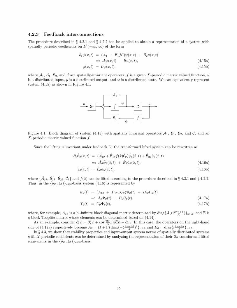
4.2.3 Feedback interconnections
The procedure described in § 4.2.1 and § 4.2.2 can be applied to obtain a representation of a system withspatially periodic coefficients on L2(−∞, ∞) of the form
∂tψ(x, t) = (A1 + B1fC)ψ(x, t) + B2u(x, t)=: Aψ(x, t) + Bu(x, t), (4.15a)
y(x, t) = Cψ(x, t), (4.15b)
where A1, B1, B2, and C are spatially-invariant operators, f is a given X-periodic matrix valued function, uis a distributed input, y is a distributed output, and ψ is a distributed state. We can equivalently representsystem (4.15) as shown in Figure 4.1.
u B2 ∫ ψ
C y
A1
fφ
B1
Figure 4.1: Block diagram of system (4.15) with spatially invariant operators A1, B1, B2, and C, and anX-periodic matrix valued function f .
Since the lifting is invariant under feedback [2] the transformed lifted system can be rewritten as
∂tψθ(x, t) = (A1θ + B1θf(x)Cθ)ψθ(x, t) + B2θuθ(x, t)
=: Aθψθ(x, t) + Bθuθ(x, t), (4.16a)
yθ(x, t) = Cθψθ(x, t), (4.16b)
where A1θ, B1θ, B2θ, Cθ and f(x) can be lifted according to the procedure described in § 4.2.1 and § 4.2.2.Thus, in the ϑθ,n(x)n∈Z-basis system (4.16) is represented by
Ψθ(t) = (A1θ + B1θΞCθ)Ψθ(t) + B2θUθ(t)=: AθΨθ(t) + BθUθ(t), (4.17a)
Yθ(t) = CθΨθ(t), (4.17b)
where, for example, A1θ is a bi-infinite block diagonal matrix determined by diagA1(i 2πn+θX )n∈Z, and Ξ is
a block Toeplitz matrix whose elements can be determined based on (4.14).As an example, consider ∂tψ = ∂2
xψ + cos( 2πX x)∂
2xψ + ∂xu. In this case, the operators on the right-hand
side of (4.17a) respectively become Aθ = (I + Γ) diag−( 2πn+θX )2n∈Z and Bθ = diagi 2πn+θ
X n∈Z.In § 4.3, we show that stability properties and input-output system norms of spatially distributed systems
with X-periodic coefficients can be determined by analyzing the representation of their Zθ-transformed liftedequivalents in the ϑθ,n(x)n∈Z-basis.
35

4.3 Stability and input-output norms of spatially periodic systems
The commutative diagram below schematically illustrates combined action of the lifting, Zθ-transform, andVθ-transform on a spatially distributed X-periodic system:
L2l2 [0, 2π) Hθ−−−−→ L2
l2 [0, 2π)
V−1θ
( )Vθ
L2L2[0, X][0, 2π) Hθ−−−−→ L2
L2[0, X][0, 2π)
Z−1θ
( )Zθ
l2L2[0, X]
H−−−−→ l2L2[0, X]
W−1X
( )WX
L2(−∞, ∞) H−−−−→ L2(−∞, ∞)
In other words, application of operator T := VθZθWX renders system (4.1) into a θ-parameterized timeinvariant family of systems of the form
Ψθ(t) = AθΨθ(t) + BθUθ(t), (4.18a)Yθ(t) = CθΨθ(t), (4.18b)
where Aθ, Bθ, and Cθ represent bi-infinite matrices that can be determined using the procedure developedin § 4.2. Therefore, the analysis of spatially distributed systems with periodic coefficients amounts to theanalysis of their T -transformed counterparts as parameter θ assumes all values in the interval [0, 2π).
We point out that systems (4.1) and (4.18) have same stability properties. This follows from the factthat operator T represents an isometric isomorphism from L2(−∞, ∞) to L2
l2 [0, 2π) and Corollary 3 of [9].Based on these, we conclude that system (4.1) is exponentially stable if and only if for each θ ∈ [0, 2π), Aθin (4.18) is stable. Additionally, it can be shown that the spectrum of the generator of (4.1) is determinedby
σA =⋃
θ∈ [0, 2π)
σAθ.
Furthermore, since WX , Zθ, and Vθ represent bijective linear isometries it follows that the T -transformpreservers system norms [2]. To illustrate this, we apply the temporal Fourier transform on (4.1) and (4.18)to obtain
y(x, ω) =[C(iωI − A)−1Bu(ω)
](x)
=: [H(ω)u(ω)] (x)
=∫ ∞
−∞H(x, ξ, ω)u(ξ, ω) dξ,
andYθ(ω) = Cθ(iωI − Aθ)−1BθUθ(ω)
=: Hθ(ω)Uθ(ω),
respectively. We remark that for any given ω, H(ω) represents a spatial operator that maps u(ω) intoy(ω). On the other hand, Hθ(ω) is a multiplication operator parameterized by two frequencies: ω ∈ R andθ ∈ [0, 2π). Properties of these two operators are closely related. For example, the H∞ norm of operator H
36

is determined by‖H‖∞ := sup
ω∈R
σmaxH(ω)= sup
θ∈ [0, 2π)
supω∈R
σmaxHθ(ω).
On the other hand, following [3] we define the H2 norm of system (4.1) as
‖H‖22 :=
12π
∫ ∞
−∞
1X
∫ X
0
trace∫ ∞
−∞H∗(x, η, ω)H(x, η, ω) dx
dη dω.
As shown at the end of this section, this quantity is determined by
‖H‖22 =
1(2π)2X
∫ 2π
0
∫ ∞
−∞trace H∗
θ (ω)Hθ(ω) dω dθ.
The H2 norm of stable systems can be obtained based on solutions of the algebraic Lyapunov equations ofthe form
AθPθ + PθA∗θ = −BθB
∗θ ,
A∗θQθ + QθAθ = −C∗
θCθ,
using either of the following two expressions:
‖H‖22 =
12πX
∫ 2π
0
tracePθC∗θCθ dθ
=1
2πX
∫ 2π
0
traceQθBθB∗θ dθ,
Results of this section are summarized in the following theorem.
Theorem 5 The feedback stability and the system norms are preserved under the transformation T :=VθZθWX . In particular, the spectrum of the generator of (4.1) is equal the spectrum of the generator of(4.18) as θ ranges over all possible values, that is
σA =⋃
θ∈ [0, 2π)
σAθ.
Furthermore, the H∞ and H2 norms of operator mapping input u into output y are determined by
‖H‖∞ = supθ∈ [0, 2π)
supω∈R
σmaxHθ(ω),
‖H‖22 =
1(2π)2X
∫ 2π
0
∫ ∞
−∞trace H∗
θ (ω)Hθ(ω) dω dθ.
In § 4.4, we illustrate how stability properties and system norms of spatially invariant systems can bealtered by connecting them in feedback with spatially periodic functions.
37

H2 norm of spatially periodic systems
Next, we derive the expression for H2 norm of system (4.1).
‖H‖22 :=
12π
∫ ∞
−∞
1X
∫ X
0
trace∫ ∞
−∞H∗(x, η, ω)H(x, η, ω) dx
dη dω
=12π
∫ ∞
−∞
1X
∫ X
0
trace
∑n∈Z
∫ (n+1)X
nX
H∗(x, η, ω)H(x, η, ω) dx
dη dω
=12π
∫ ∞
−∞
1X
∫ X
0
trace
∑n∈Z
∫ X
0
H∗(nX + x, η, ω)H(nX + x, η, ω) dx
dη dω
=12π
∫ ∞
−∞
1X
∫ X
0
trace
∑n∈Z
∫ X
0
H∗n(x, η, ω)Hn(x, η, ω) dx
dη dω
=12π
∫ ∞
−∞
1X
∫ X
0
trace
∑n∈Z
∫ X
0
H∗n(x, η, ω)
12π
∫ 2π
0
Hθ(x, η, ω)eiθn dθ dx
dη dω
=1
(2π)2X
∫ 2π
0
∫ ∞
−∞trace
∫ X
0
∫ X
0
(∑n∈Z
Hn(x, η, ω)e−iθn
)∗Hθ(x, η, ω) dx dη
dω dθ
=1
(2π)2X
∫ 2π
0
∫ ∞
−∞trace
∫ X
0
∫ X
0
H∗θ(x, η, ω)Hθ(x, η, ω) dx dη
dω dθ
=:1
(2π)2X
∫ 2π
0
∫ ∞
−∞‖Hθ(ω)‖2
HS dω dθ
=1
(2π)2X
∫ 2π
0
∫ ∞
−∞‖V−1
θ Hθ(ω)Vθ‖2HS dω dθ
=1
(2π)2X
∫ 2π
0
∫ ∞
−∞‖Hθ(ω)‖2
HS dω dθ
=1
(2π)2X
∫ 2π
0
∫ ∞
−∞trace H∗
θ (ω)Hθ(ω) dω dθ.
4.4 Examples of PDEs with periodic coefficients
In this section, we illustrate how stability properties and system norms of PDEs can be changed by intro-ducing feedback terms with spatially periodic coefficients. Our results reveal that, depending on the valuesof amplitude and frequency of a periodic gain, both stability and input-output gains of the original equationcan be modified. This phenomenon is referred to as ‘parametric resonance’ and is encountered in manyproblems of physical significance. Furthermore, we show how our results can lead to an analytic expressionfor the eigenvalues of the underlying operators, for a special class of PDEs with periodic coefficients.
First example
In [10], the periodic solutions of the Ginzburg-Landau (GL) equation are studied. This equation results fromnonlinear stability theory and appears in the analysis of many relevant fluid mechanics problems: the Benardproblem, the Taylor problem, Tollmien-Schlichting waves, gravity waves, etc. (for more details see [10] andreferences therein). It is worth mentioning that the GL equation describes the evolution of a slowly varyingcomplex amplitude of a neutral plane wave.
The linearization of this equation around its limit cycle solution φ0 := f(x) exp (iΩt), f(x) = f(x+X),results in a PDE with periodic coefficients of the form
∂tφ = z1φ + z2∂2xφ + z3(2|f |2φ+ f2φ∗), (4.19)
where φ∗ is the complex-conjugate of a field φ, and z1 := ρ− iΩ, z2 := c0 + i, z3 := i− ρ, with c0, Ω, and ρ
38

being real valued parameters. Furthermore, ρ := c0/c1, 0 ≤ c20 ≤ c1.If we introduce the following notation
ψ :=[φφ∗
], (4.20)
we can rewrite (4.19) as
∂tψ := A(∂x)ψ, (4.21)
where the operator A is given by
A :=[z1 + z2∂
2x + 2z3|f |2 z3f
2
(z3f2)∗ z∗1 + z∗2∂2x + 2z∗3 |f |2
].
Clearly, A can be separated into a sum of a spatially invariant operator and a matrix-valued periodic function,which lends itself to the application of the results derived in § 4.2. We use these results for a numericalapproximation of A and investigate its eigenvalues. In particular, we assume f(x) := α cos( 2π
X x) and considera problem of the stability of system (4.19). We note that in this case (4.19) cannot be interpreted as thelinearized GL equation since φ0, for the above given f(x), is no longer a limit cycle solution of the nonlinearGL equation. Nevertheless, this problem is worth investigating because it represents an example of a systemwhose stability can be changed by feedback terms with spatially periodic gains.
Figure 4.2 illustrates the maximal real part of the operator A eigenvalues, λ(A), as a function of α andX, for c0 = 0.4, ρ = 0.4, and Ω = 5. It can be readily shown that for α = 0, max (Reλ(A)) = ρ = 0.4,which means that system (4.19) is open-loop unstable. Clearly, ‘closing a loop’, by introducing the spatiallyperiodic gains in feedback, changes the value of max (Reλ(A)) significantly, as illustrated in the left plotof Figure 4.2.
Figure 4.2 also shows max (Reλ(A)) as a function of α for X ≈ 1.31. The right plot in this figurefurther illustrates the previously mentioned changes in max (Reλ(A)), and reveals an interesting featureof this example. Namely, the regions of instability and stability repeat in an alternating arrangement forcertain values of the amplitude α.
05
10 02
46
8
−35
−30
−25
−20
−15
−10
−5
0
Xα
max
(R
eλ(
A)
)
0 2 4 6 8 10
−8
−6
−4
−2
0
2
α
max
(Re
λ(A)
)
Figure 4.2: Left plot: max (Reλ(A)) as a function of α and X for f(x) := α cos( 2πX x), c0 = 0.4, ρ = 0.4,
and Ω = 5. Right plot: max (Reλ(A)) as a function of α for f(x) := α cos( 2πX x), X ≈ 1.31, c0 = 0.4,
ρ = 0.4, and Ω = 5.
Second example
In [11], a class of nonlinear PDEs with periodic plane wave solutions including forms of the Schrodinger andgeneralized KdV equations is considered. The linearization of these equations around a plane wave yields
39

the following PDE with periodic coefficients:
∂tφ(x, t) = p(∂x)φ(x, t) + αe2i 2πX xφ∗(x, t), (4.22)
where p is a polynomial with complex coefficients, and α is a complex scalar. We can define the state by(4.20), which transforms (4.22) into (4.21), with
A :=[
A11 A12
A21 A22
]:=
[p(∂x) αe2i( 2π
X )x
α∗e−2i( 2πX )x p∗(∂x)
].
Operator A can be separated into a sum of a spatially invariant operator and a matrix-valued periodicfunction, and the previously described procedure transforms (4.21) into
Ψθ(t) = AθΨθ(t). (4.23)
Bi-infinite Toeplitz matrices Aθ12 and Aθ21 are defined in (4.14) with the elements of Aθ12 given by
am =
α m = 2,0 otherwise,
(4.24)
and the elements of Aθ21 given by
am =
α∗ m = −2,0 otherwise.
(4.25)
Furthermore, if we define pn(θ) := p(i 2πn+θX ), then
Aθ11 = diagpn(θ)n∈Z, Aθ22 = diagp∗n(θ)n∈Z.
The eigenvalues of Aθ are computed by defining Gθ := λI −Aθ and using the formula
det(Gθ) = det(Gθ11) det(Gθ22 −Gθ21G−1θ11Gθ12).
Noting that Gθ12 and Gθ21 are just scaled backward and forward shift operators, respectively, then det(λI−Aθ) is computed to be
∏n∈Z
(λ− pn(θ))∏n∈Z
(λ− p∗n(θ) −|α|2
λ− pn−2(θ)) =∏
n∈Z
(λ − pn−2(θ)) (λ − p∗n(θ)) − |α|2
,
which yields the eigenvalues λn(θ) of Aθ equal to
12pn−2(θ) + p∗n(θ) ±
√4|α|2 + (pn−2(θ) − p∗n(θ))
2.
This result can be applied to the nonlinear Schrodinger equation
i ∂tϕ(z, t) = − ∂2zϕ(z, t) − V (ϕϕ∗)ϕ(z, t), (4.26)
with potential V (φφ∗) that satisfies the dispersion equation V (a2) = (2πX )2 − ( 2π
T )2. As illustrated in [11],(4.26) exhibits a periodic plane wave solution aei( 2π
X z− 2πT t). The linearization of (4.26) around this solution,
together with a coordinate transformation of the form x := z − XT t, yields (4.22) with
p(∂x) := XT ∂x + i
(∂2x + V (a2) + a2V ′(a2)
),
α := ia2V ′(a2).
40

It is readily shown, using the previously derived formula for λn(θ), that the generator of (4.22) has purelyimaginary eigenvalues if and only if V ′(a2) ≤ 0. On the other hand, if V ′(a2) > 0 then there exist aneigenvalue of A with a positive real part. The same conclusion has been derived in [11] using the techniquewhich is well-suited for systems that can be represented by (4.22). It is worth noting that the spatio-temporal lifting can be used for analysis of stability and input-output norms of general linear PDEs withperiodic coefficients on L2(−∞, ∞).
Third example
In this subsection, by means of an example, we illustrate how system norms of spatially invariant systemscan be changed by combining them in feedback with spatially periodic gains. In particular, we consider asystem of the form
∂t
[ψ1(x, t)ψ2(x, t)
]=
[− c + ∂xx − f(x)q + f(x) − c + ∂xx
] [ψ1(x, t)ψ2(x, t)
]+
[I 00 I
] [u1(x, t)u2(x, t)
], (4.27a)
[y1(x, t)y2(x, t)
]=
[I 00 I
] [ψ1(x, t)ψ2(x, t)
], (4.27b)
where c and q are positive and non-negative real numbers, respectively, f(x) := α cos( 2πX x), α ∈ R, and
x ∈ R. If α ≡ 0, system (4.27) represent a linear spatially invariant system. In this case, using the toolsof [9] it can be easily established that system (4.27) is exponentially stable with H∞ norm given by
‖H‖2∞ =
1
c2 + 0.5(q2 − q
√q2 + 4c2
) .Our objective is to investigate the dynamical properties of system (4.27) for α = 0.
The derivative of the following Lyapunov function candidate along the solutions of unforced system (4.27a)
V (ψ1, ψ2) :=12〈ψ1, ψ1〉 +
12〈ψ2, ψ2〉 ,
is determined by
V (ψ1, ψ2) = 〈ψ1, ∂tψ1〉 + 〈ψ2, ∂tψ2〉= 〈ψ1,− cψ1 + ∂xxψ1 − fψ2〉 + 〈ψ2, qψ1 + fψ1 − cψ2 + ∂xxψ2〉= − c 〈ψ1, ψ1〉 − c 〈ψ2, ψ2〉 − 〈∂xψ1, ∂xψ1〉 − 〈∂xψ2, ∂xψ2〉 + q 〈ψ2, ψ1〉≤ − (c − q
2) 〈ψ1, ψ1〉 − (c − q
2) 〈ψ2, ψ2〉 − 〈∂xψ1, ∂xψ1〉 − 〈∂xψ2, ∂xψ2〉 ,
which implies the negative definiteness of V along the solutions of unforced system (4.27a) as long asparameters c and q are such that q < 2c. Therefore, the stability properties of the original spatially invariantsystem are not influenced by the periodic feedback if the coupling between the two subsystems in (4.27a)is small enough (that is, q < 2c). This estimate may be very conservative but it is important that wehave established stability for certain values of parameters q and c irrespective of the values that period andamplitude of the periodic gain assume. This allows us to select the pair (q, c) to guarantee stability of (4.27a)and investigate the dependence of the input-output norms of (4.27) on both α and X.
The left plot in Figure 4.3 illustrates the dependence of the H∞ norm of system (4.27) on both amplitudeand period of spatially periodic gain for c = 1 and q = 0.5. The right plot in the same figure shows howH∞ norm of (4.27) changes with X at α = 15. We note that at α = 0 H∞ norm is equal to 1.28 whichcorresponds to the value determined for the spatially invariant system. As our results indicate, even thoughthe stability properties of system (4.27) are not changed by introducing the spatially periodic feedback, itspresence has a beneficial influence on the input-output system gains. We remark that this fact cannot beestablished by the existing tools, e.g. Floquet analysis of periodic PDEs, because this type of analysis does
41

not easily lend itself to the computation of system norms. To this end, we have developed the procedure thatcan be used to compute both the spectrum of the generating operator and H2 and H∞ norms of spatiallydistributed systems with periodic coefficients.
0
5
10 05
1015
0
0.5
1
1.5
αX
|| H
||∞
0 2 4 6 8 100
0.2
0.4
0.6
0.8
1
1.2
1.4
X
|| H
||∞
Figure 4.3: The dependence of the H∞ norm of system (4.27) with c = 1, q = 0.5 on amplitude and periodof spatially periodic feedback (left plot), and period for α = 15 (right plot).
4.5 Extensions
The developed procedure can be also used to investigate dynamical properties of systems of the form
∂tψ(x, z, t) = Aψ(x, z, t) + Bu(x, z, t),y(x, z, t) = Cψ(x, z, t),
where A, B, and C are time invariant linear operators with spatially periodic coefficients in x ∈ R, whereasz belongs to a set of indices with no predefined structure. As an example, consider the following equation
∂tψ(x, z, t) = (∂zz + ∂xx + f(x))ψ(x, z, t) + u(x, z, t),y(x, z, t) = ψ(x, z, t),
(4.29)
with z ∈ [− 1, 1], ψ(x,±1, t) = 0, and f(x) = f(x + X). Using the results of § 4.2, system (4.29) can betransformed into a θ-parameterized family of PDEs of the form
∂tΨθ(z, t) = (∂zz + Dθ + Γ)Ψθ(z, t) + Uθ(z, t),Yθ(z, t) = Ψθ(z, t),
(4.30)
where θ ∈ [0, 2π), Dθ := diag− ( 2πn+θX )2n∈Z, and Γ is a Toeplitz matrix determined by (4.14). It is not
difficult to show that systems (4.29) and (4.30) have equivalent stability properties and input-output norms.
4.6 Summary
We develop a framework for analysis of stability and input-output norms of distributed systems with spatiallyperiodic coefficients. It is shown that the main ideas of a well known temporal lifting technique for linearperiodic ODEs are readily extendable to PDEs in which certain coefficients are spatially periodic functions.A particular basis set is used to obtain convenient representations of transformed lifted signals and spatiallyperiodic systems. It is also illustrated, by means of three examples, how stability properties and input-outputnorms of spatially invariant PDEs can be changed when a spatially periodic feedback is introduced.
42

Bibliography
[1] V. I. Arnold, Mathematical Methods of Classical Mechanics. Springer-Verlag, 1989.
[2] B. Bamieh and J. B. Pearson, “A general framework for linear periodic systems with applications toH∞ sampled-data control,” IEEE Transactions on Automatic Control, vol. 37, no. 4, pp. 418–435, April1992.
[3] ——, “The H2 problem for sampled-data systems,” Systems and Control Letters, vol. 19, no. 1, pp.1–12, July 1992.
[4] B. Bamieh, M. A. Dahleh, and J. B. Pearson, “Minimization of the L∞-induced norm for sampled-datasystems,” IEEE Transactions on Automatic Control, vol. 38, no. 5, pp. 717–732, May 1993.
[5] Y. Yamamoto, “A function space approach to sampled data control systems and tracking problems,”IEEE Transactions on Automatic Control, vol. 39, no. 4, pp. 703–713, April 1994.
[6] T. Hagiwara and M. Araki, “FR-operator approach to the H2 analysis and synthesis of sampled-datasystems,” IEEE Transactions on Automatic Control, vol. 40, no. 8, pp. 1411–1421, August 1995.
[7] T. Chen and B. Francis, Optimal Sampled-Data Control Systems. Springer, 1995.
[8] G. E. Dullerud, Control of Uncertain Sampled-Data Systems. Birkhauser, 1996.
[9] B. Bamieh, F. Paganini, and M. A. Dahleh, “Distributed control of spatially invariant systems,” IEEETransactions on Automatic Control, vol. 47, no. 7, pp. 1091–1107, July 2002.
[10] L. Sirovich and P. K. Newton, “Periodic solutions of the Ginzburg-Landau equation,” Physica 21D, pp.115–125, 1986.
[11] P. K. Newton and J. B. Keller, “Stability of periodic plane waves,” SIAM J. Appl. Math., vol. 47, no. 5,pp. 959–964, October 1987.
43

Chapter 5
Conclusions and future directions
Conclusions
We introduce an explicit procedure for determination of the frequency responses for a class of P(I)DEs with, ingeneral, non-normal dynamical generators and non-constant coefficients in the spatially independent variable.The motivation for this problem arises from the observation that the eigenvalue-based stability analysis ofnon-normal dynamical systems often leads to erroneous conclusions. Namely, these systems can exhibit largetransient responses (i.e., behave as unstable on finite time intervals) even in the absence of exponentiallygrowing system modes. In view of this, it is relevant to develop efficient schemes for determining appropriatelydefined measures of transient amplification.
Instead of usual finite dimensional approximations of the underlying operators, we derive an explicitformula for the power spectral density of the frequency response operator. This formula only involves finitedimensional computations with matrices whose dimension is at most four times larger than the order of theunderlying generators. Thus, we perform an exact reduction of an infinite dimensional problem to a finitedimensional problem.
We also develop a framework for analysis of internal and input-output properties of PDEs with spatiallyperiodic coefficients. We demonstrate that the main ideas of a well known temporal lifting technique forlinear periodic ODEs can be extended to PDEs in which certain coefficients are spatially periodic functions.A particular basis set is used to obtain convenient representations of transformed lifted signals and spatiallyperiodic systems. We also illustrate how stability and input-output norms of spatially invariant PDEs canbe modified when a spatially periodic feedback is introduced.
Several open research problems are given below.
Future directions
Application of the exact formula for Hilbert–Schmidt norm of frequency response operator toproblems with non-constant coefficients. All examples in this dissertation illustrate explicit determina-tion of frequency responses for problems with constant coefficients in the spatially independent variable. Wealso plan to apply the formula for Hilbert–Schmidt norm of frequency response operator to problems withnon-constant coefficients. This will require determination of the state transition matrices in (3.18), whichnecessitates solving certain differential equations. In particular, frequency response operator of a systemthat describes the dynamics of velocity fluctuations in channel fluid flows linearized around velocity profileU(y) = 1 − y2 has a TPBVSR with non-constant coefficients in y.
Exact determination of maximal singular values of the frequency response operator. We intendto determine maximal singular values of the frequency response operator from its TPBVSR. These singularvalues, at any frequency, quantify the largest amplification of deterministic disturbances.
Identification of classes of PDEs in which parametric resonance can occurs. Recently, Fardad &
44

Bamieh [1] employed methodology developed in this dissertation and perturbation analysis to show how todesign a spatially periodic perturbation to stabilize a marginally stable PDE. It was established that, upto first order in the perturbation parameter, parametric resonance can only occur at the isolated frequencytwice larger than the frequency of the marginally-stable mode of the unperturbed system. Investigationsalong these lines will elucidate classes of spatially distributed systems in which parametric resonance cantake place.
45

Bibliography
[1] M. Fardad and B. Bamieh, “A perturbation analysis of parametric resonance and periodic control inspatially distributed systems,” 2004, submitted to the 43rd IEEE Control and Decision Conference.
46
Part II
Modeling and analysis of transitionand turbulence in channel flows
47

Chapter 6
Background
The basic theoretical issues related to the study of transition to turbulence can be divided into two categories:
• Explaining why the laminar-turbulent transition takes place.
• Determining the dominant structures of flow perturbations that lead to the transition.
The classical approach to this problem involves the spectral (that is, normal mode) analysis of the NSequations linearized around certain laminar flow condition. For low Reynolds numbers all flows are stable [1–3], and classical analysis is thus concerned with finding the critical Reynolds numbers at which exponentiallygrowing normal modes appear, or equivalently, identifying when the generator of the evolution equationbecomes unstable. The predictions of these investigations agree fairly well with the experimental results inmany relevant flows: e.g., those driven mainly by centrifugal and thermal forces [4]. However, in the veryimportant case of shear flows in streamlined geometries, classical theory fails to predict both the transitionReynolds numbers and the dominant flow structures that accompany the transition. For example, planeCouette flow is stable for all values of the Reynolds number [5], and plane Poiseuille flow losses stabilityonly if the Reynolds number becomes larger than approximately 5772 [6]. However, the experiments telldifferent story: the transition is observed to take place as early as R ≈ 350 in Couette flow [7, 8], and asearly as R ≈ 1000 in Poiseuille flow [9]. Furthermore, the transition Reynolds numbers strongly depend onthe experimental conditions. By comparing different experimental results for plane Poiseuille flow, the widevariation in transition Reynolds numbers from 266 [10] to 8000 [11] was observed in [9]. In the former case,the early transition was due to a noisy environment created by a non-smooth inlet contraction. On the otherhand, the latter example demonstrates that under carefully controlled experiments the transition may nottake place even for flows that are unstable according to the classical hydrodynamic stability theory. Thisindicates that the concept of stability/instability in the classical sense may be too narrow to capture thenotion of transition.
For wall bounded shear flows, the classical hydrodynamic stability analysis leads to transition theoriesbased on the well known Tollmien-Schlichting (TS) waves, which have long been considered to be the primarymechanism of instability leading to transition. TS waves represent the eigenfunctions corresponding to the‘poorly damped’ system modes (that is, the eigenvalues in the immediate vicinity of the imaginary axis),and they can only be observed in carefully controlled experiments with very little background noise. Also,TS waves have been considered to be the first step in a transition scenario that leads to three-dimensional‘secondary’ instabilities [12–14]. This scenario leaves many unanswered questions, as Herbert [13] observed:
‘In noisy environments, however, the TS mechanism is no longer needed and may be bypassed;preexisting vorticity concentration of irregular spacing and orientation combined with the meanshear directly activate the process of vortex tilting and stretching [14] that lead to transition.’
Indeed, the secondary instability theory is quite unsatisfactory for describing experimentally observed phe-nomena in so-called natural transition [15]. Unless in carefully controlled experiments, the transitionReynolds numbers, as well as the dominant flow structures, are not related to TS waves [9, 11,15–19].
48

We approach this problem by analyzing the dynamical properties of the Navier-Stokes (NS) equationswith spatially distributed and temporally varying body force fields. These fields are considered as inputs,and various combinations of the resulting velocity and vorticity fields are considered as outputs. This input-output analysis can in principle be done in any geometry and for the full nonlinear NS equations. In suchgenerality however, it is difficult to obtain useful results. We therefore concentrate on the geometry ofchannel flows, and the input-output dynamics of the LNS equations.
The analysis of dynamical systems with inputs has a long history in circuit theory, controls, communica-tions, and signal processing. In this analysis, it is convenient to express dynamical systems as input-output‘blocks’ that can be connected together in a variety of cascade, series, and feedback arrangements. Theutility of this approach is twofold. First, it greatly facilitates engineering analysis and design of complexsystems made up of sub-blocks that are easier to characterize. Second, it allows for modeling dynamicalinputs which are unmeasurable or uncertain. These include stochastic or deterministic uncertain signals suchas noise or uncertain forcing that are inevitably present in most physical systems.
The terminology here might be a little confusing. While we are concerned with the dynamical behaviorof the linearized NS equations, input-output analysis of the LNS is related but not equivalent to linearhydrodynamic stability analysis. As already mentioned, in the latter, the objective is to characterize ex-ponentially growing (unstable) normal modes. As we will illustrate, input-output analysis reveals unstablenormal modes, as well as transient growth, disturbance amplification, and so-called pseudo-spectral modes.This analysis has very close mathematical connections with work on transient energy growth (also known asnon-normal growth) [20–22], pseudo-spectral analysis [4], and amplification of stochastic excitations [23,24].In some sense, it can also be considered as a type of receptivity analysis, though this connection is morequalitative in nature. Rather than study the receptivity of a boundary layer to upstream or free streamdisturbances as is commonly done [25–27], our input-output analysis is the receptivity of channel flows tospatially and temporally distributed body forces. The latter is mathematically and computationally moretractable, yet appears to have many of the qualitative features of boundary layer receptivity analysis.
Our work is greatly influenced by recent research in what has become known as transient growth mech-anisms for bypass transitions [4, 20–24,28–33]. We will only briefly outline some of the more closely relatedwork here, and refer the reader to the recent monograph [3] and the references therein for a fuller discussion.The main point of departure of this work from classical linear hydrodynamic stability is the fact that thelatter is concerned solely with the existence of exponentially growing modes. In other words, it is essen-tially an asymptotic analysis of infinite time limits. In certain flows however, transient (that is, finite-time)phenomena appear to play a significant role. While the possibility of transient growth has long been recog-nized [34], it is only in the past two decades that effective mathematical methods have been used to analyzeit. In [21,22] initial states with the largest transient energy growth in subcritical flows were discovered usinga singular value analysis. These ‘worst case’ initial states lead to flow structures that resemble streamwisevortices and streaks. A somewhat different analysis is done by computing the pseudo-spectrum rather thanthe spectrum of the generating dynamics [4], and the most unstable pseudo-spectral modes turn out tobe related to streamwise vortices and streaks. A third analysis method [23, 24] studies the most energeticresponse of the linearized Navier-Stokes equations to stochastic excitation. Yet again, the most energeticallyexcited flow structures appear to resemble streamwise vortices and streaks. The common theme between thethree methods is that a certain norm of the perturbed flow state is used (namely kinetic energy density),and the responses with respect to various types of uncertainties are analyzed.
A streamwise vortex represents an elongated region of vorticity, and a streamwise streak represents anelongated region of high and low velocity perturbations. Both these structures are approximately alignedwith the direction of nominal flow U(y), and they are commonly observed in experimental investigationsrelated to transition in channel and boundary layer flows [9, 15,18,19,35].
Previous work on ‘non-normal growth’ has tended to emphasize transient energy growth as a mechanismthat might lead to exiting a region of attraction of the full nonlinear Navier-Stokes equations. In this thesishowever (and similarly in [23, 24]), we adopt a different perspective in which the LNS are considered withuncertain body forces, initial conditions are zero, and thus flow field perturbations are solely due to excitationby body forces. We show that the effects of these body forces on flow perturbations scale badly with theReynolds number. Depending on the polarization of the force and how flow perturbations are measured,these effects scale with R, R2, R3, or R4. Thus, for large enough Reynolds numbers, the effects of even tiny
49

body forces will become appreciable. It is not difficult to argue that any flow condition has some degree ofuncertainty in either flow geometry, base profile, and/or non-flat walls. In carefully controlled experiments,these uncertainties may be very small. However, it appears that the NS equations (both the linearized andfull versions) in wall-bounded shear flows are exceedingly sensitive to small amounts of such uncertainty.It is thus important to analyze the equations while taking such uncertainties into account. We borrowheavily from the field of Robust Control theory [36], where mathematical tools for the analysis and controlof uncertain dynamical systems have been developed. Indeed, several researches [37–41] have been successfulin designing linear controllers based on these methods either for the LNS or nonlinear flow dynamics inDirect Numerical Simulations (DNS).
This part of the thesis is organized as follows: in Chapter 7, we discuss externally excited LNS equationsin channel flows. These equations determine a dynamical description of flow fluctuations subject to spatiallydistributed and temporally varying body force fields. In Chapter 8, we present the spatio-temporal frequencyresponses in Poiseuille, Couette, and a turbulent mean flow profile. One of our main objectives is to illustratethe input-output resonances from forcing inputs in different directions to different components of the velocityfield. The most amplified input-output resonances turn out to resemble streamwise vortices and streaks andoblique waves. A comparison between them and internal resonances (TS waves) is given using the frequencyresponse. This is done for both subcritical and supercritical flows, where the latter are analyzed with theappropriate exponential discounts on their energies. One of our other conclusions is that the spanwise andwall-normal forces are much more influential on flow perturbations than the streamwise force. Furthermore,the impact of these forces is most powerful on the streamwise velocity component. Analytical explanationsfor these observations as well as formulae for the dependence of these influences on the Reynolds numberare given in Chapter 9, where we also study the effectiveness of the near-wall inputs for streamwise constantthree-dimensional perturbations. We analytically demonstrate that the spanwise direction force has, by far,the biggest impact on the evolution of the velocity field components. These facts were recently observedin experimental and numerical studies of flow control using the Lorentz force [42–46]. In Chapter 10, westudy the spatio-temporal impulse responses of the LNS in subcritical Poiseuille flow with R = 2000. Thefirst motivation for this problem comes from experimental work, where transition is observed to occur eithernaturally, with so-called ‘turbulent spots’, or when these spots are intentionally induced in the flow bydeliberate external excitation, which can be modelled as a spatio-temporal impulse body force in the NSequations. We show that the impulse responses of the LNS system display some of the qualitative featuresof early stages of turbulent spots observed in experiments and full direct numerical simulations. Anothermotivation is to fully probe the dynamics of the linearized equations. We find that these equations exhibitrich and complex structures hitherto unseen by other linear analysis methods.
50

Bibliography
[1] D. D. Joseph, Stability of Fluid Motions I. Springer-Verlag, 1976.
[2] P. G. Drazin and W. H. Reid, Hydrodynamic Stability. Cambridge University Press, 1981.
[3] P. J. Schmid and D. S. Henningson, Stability and Transition in Shear Flows. New York: Springer-Verlag, 2001.
[4] L. N. Trefethen, A. E. Trefethen, S. C. Reddy, and T. A. Driscoll, “Hydrodynamic stability withouteigenvalues,” Science, vol. 261, pp. 578–584, 1993.
[5] V. A. Romanov, “Stability of plane-parallel Couette flow,” Funct. Anal. Applics., vol. 7, pp. 137–146,1973.
[6] S. A. Orszag, “Accurate solution of the Orr-Sommerfeld equation,” J. Fluid Mech., vol. 50, pp. 689–703,1971.
[7] N. Tillmark and P. H. Alfredsson, “Experiments on transition in plane Couette flow,” J. Fluid Mech.,vol. 235, pp. 89–102, 1992.
[8] O. Dauchot and F. Daviaud, “Finite amplitude perturbation and spots growth mechanism in planeCouette flow,” Physics of Fluids, vol. 7, no. 2, pp. 335–343, 1995.
[9] D. R. Carlson, S. E. Widnall, and M. F. Peeters, “A flow-visualization study of transition in planePoiseuille flow,” J. Fluid Mech., vol. 121, pp. 487–505, 1982.
[10] S. J. Davies and C. M. White, “An experimental study of the flow of water in pipes of rectangularsection,” Proc. R. Soc. Lond. A, vol. 119, no. 781, pp. 92–107, 1928.
[11] M. Nishioka, S. Iida, and Y. Ichikawa, “An experimental investigation of the stability of plane Poiseuilleflow,” J. Fluid Mech., vol. 72, pp. 731–751, 1975.
[12] S. A. Orszag and A. T. Patera, “Secondary instability of wall-bounded shear flows,” J. Fluid Mech.,vol. 128, pp. 347–385, 1983.
[13] T. Herbert, “Secondary instability of boundary layers,” Ann. Rev. Fluid Mech., vol. 20, pp. 487–526,1988.
[14] B. J. Bayly, S. A. Orszag, and T. Herbert, “Instability mechanisms in shear flow transition,” Ann. Rev.Fluid Mech., vol. 20, pp. 359–391, 1988.
[15] B. G. B. Klingmann, “On transition due to three-dimensional disturbances in plane Poiseuille flow,” J.Fluid Mech., vol. 240, pp. 167–195, 1992.
[16] P. S. Klebanoff, K. D. Tidstrom, and L. M. Sargent, “The three-dimensional nature of boundary-layerinstability,” J. Fluid Mech., vol. 12, pp. 1–34, 1962.
[17] F. W. Chambers and A. S. W. Thomas, “Turbulent spots, wave packets, and growth,” Physics of Fluids,vol. 26, no. 5, pp. 1160–1162, 1983.
51

[18] F. Alavyoon, D. S. Henningson, and P. H. Alfredsson, “Turbulent spots in plane Poiseuille flow - flowvisualization,” Physics of Fluids, vol. 29, no. 4, pp. 1328–1331, 1986.
[19] M. Matsubara and P. H. Alfredsson, “Disturbance growth in boundary layers subjected to free-streamturbulence,” J. Fluid Mech., vol. 430, pp. 149–168, 2001.
[20] L. H. Gustavsson, “Energy growth of three-dimensional disturbances in plane Poiseuille flow,” J. FluidMech., vol. 98, p. 149, 1991.
[21] K. M. Butler and B. F. Farrell, “Three-dimensional optimal perturbations in viscous shear flow,” Physicsof Fluids A, vol. 4, p. 1637, 1992.
[22] S. C. Reddy and D. S. Henningson, “Energy growth in viscous channel flows,” J. Fluid Mech., vol. 252,pp. 209–238, 1993.
[23] B. F. Farrell and P. J. Ioannou, “Stochastic forcing of the linearized Navier-Stokes equations,” Physicsof Fluids A, vol. 5, no. 11, pp. 2600–2609, 1993.
[24] B. Bamieh and M. Dahleh, “Energy amplification in channel flows with stochastic excitation,” Physicsof Fluids, vol. 13, no. 11, pp. 3258–3269, 2001.
[25] M. E. Goldstein and L. S. Hultgren, “Boundary-layer receptivity to long-wave free-stream disturbances,”Annual Review of Fluid Mechanics, vol. 21, pp. 137–166, 1989.
[26] D. C. Hill, “Adjoint systems and their role in the receptivity problem for boundary layers,” J. FluidMech., vol. 292, pp. 183–204, 1995.
[27] P. Luchini and A. Bottaro, “Gortler vortices: a backward-in-time approach to the receptivity problem,”J. Fluid Mech., vol. 363, pp. 1–23, 1998.
[28] B. F. Farrell and P. J. Ioannou, “Perturbation growth in shear flow exhibits universality,” Physics ofFluids A, vol. 5, no. 9, pp. 2298–2300, 1993.
[29] ——, “Variance maintained by stochastic forcing of non-normal dynamical systems associated withlinearly stable flows,” Physical Review Letters, vol. 72, no. 8, pp. 1188–1191, 1994.
[30] S. C. Reddy, P. J. Schmid, J. S. Baggett, and D. S. Henningson, “On stability of streamwise streaksand transition tresholds in plane channel flows,” J. Fluid Mech., vol. 365, pp. 269–303, 1998.
[31] P. Luchini, “Reynolds-number-independent instability of the boundary layer over a flat surface: optimalperturbations,” J. Fluid Mech., vol. 404, pp. 289–309, 2000.
[32] S. J. Chapman, “Subcritical transition in channel flows,” J. Fluid Mech., vol. 451, pp. 35–97, 2002.
[33] A. Bottaro, P. Corbett, and P. Luchini, “The effect of base flow variation on flow stability,” J. FluidMech., vol. 476, pp. 293–302, 2003.
[34] W. M. F. Orr, “The stability or instability of the steady motions of a perfect liquid and of a viscousliquid. Part I: A perfect liquid. Part II: A viscous liquid,” Proc. R. Irish Acad. A, vol. 27, pp. 9–138,1907.
[35] M. Asai and M. Nishioka, “Origin of the peak-valley wave structure leading to wall turbulence,” J. FluidMech., vol. 208, pp. 1–23, 1989.
[36] K. Zhou, J. C. Doyle, and K. Glover, Robust and Optimal Control. Prentice Hall, 1996.
[37] T. R. Bewley and S. Liu, “Optimal and robust control and estimation of linear paths to transition,” J.Fluid Mech., vol. 365, pp. 305–349, 1998.
52

[38] K. H. Lee, L. Cortelezzi, J. Kim, and J. Speyer, “Application of reduced-order controller to turbulentflows for drag reduction,” Physics of Fluids, vol. 13, no. 5, pp. 1321–1330, 2001.
[39] J. Kim, “Control of turbulent boundary layers,” Physics of Fluids, vol. 15, no. 5, pp. 1093–1105, 2003.
[40] M. Hogberg, T. R. Bewley, and D. S. Henningson, “Linear feedback control and estimation of transitionin plane channel flow,” J. Fluid Mech., vol. 481, pp. 149–175, 2003.
[41] ——, “Relaminarization of Reτ = 100 turbulence using linear state-feedback control,” Physics of Fluids,vol. 15, no. 11, pp. 3572–3575, 2003.
[42] C. Henoch and J. Stace, “Experimental investigation of a salt water turbulent boundary layer modifiedby an applied streamwise magnetohydrodynamic body force,” Physics of Fluids, vol. 7, no. 6, pp. 1371–1383, 1995.
[43] C. H. Crawford and G. E. Karniadakis, “Reynolds stress analysis of EMHD-controlled wall turbulence.Part I. Streamwise forcing,” Physics of Fluids, vol. 9, no. 3, pp. 788–806, 1997.
[44] T. W. Berger, J. Kim, C. Lee, and J. Lim, “Turbulent boundary layer control utilizing the Lorentzforce,” Physics of Fluids, vol. 12, no. 3, pp. 631–649, 2000.
[45] Y. Du and G. E. Karniadakis, “Suppressing wall turbulence by means of a transverse traveling wave,”Science, vol. 288, pp. 1230–1234, 2000.
[46] Y. Du, V. Symeonidis, and G. E. Karniadakis, “Drag reduction in wall-bounded turbulence via atransverse travelling wave,” J. Fluid Mech., vol. 457, pp. 1–34, 2002.
53

Chapter 7
Dynamical description of flowfluctuations
Any real fluid flow is accompanied with certain imperfections that cause the velocity and pressure fields todeviate from their nominal values. These imperfections are typically difficult to model, and they may arise dueto, for example, surface roughness or incoming stream irregularities. The purpose of this chapter is to developthe appropriate mathematical framework for studying the dynamics of flow fluctuations around certainnominal flow conditions. We confine our attention to the incompressible shear flows through plane channelswith unidirectional parallel nominal velocity profiles that depend only on the wall-normal coordinate. Thetypical examples of these flows are given by plane Poiseuille flow (flow with a parabolic nominal velocityprofile; this flow is also referred to as the plane channel flow), and plane Couette flow (flow with a linearnominal velocity profile; this flow is also referred to as the linear shear flow).
The problem of transition to turbulence in these particular flow geometries is central to the technologicallyimportant problem of skin friction drag reduction. Despite fairly simple geometrical configurations, theproblem of transition in these flows has historically been most difficult to model. We approach this problemby accounting explicitly for signal uncertainty in the NS equations. Namely, we model the fluid flow in thepresence of body force fields which we consider to be ‘external’ inputs or excitations in these equations. Thesources of these additional ingredients in the NS equations can be the aforementioned imperfections in thegeometry and/or incoming stream. In this framework, spatially distributed and temporally varying bodyforce fields are considered as inputs, whereas various combinations of the resulting velocity and/or vorticityfields are considered as outputs.
7.1 Linearized Navier-Stokes equations
We consider three-dimensional flow between two parallel infinite plates. Figure 7.1 illustrates geometry inplane Poiseuille flow. Incompressible flow of a viscous Newtonian fluid satisfies the NS equations and thecontinuity equation given in their non-dimensional form by
∂tu = − ∇uu − ∇p +1R
∆u, (7.1a)
0 = ∇·u, (7.1b)
where u is the velocity vector, p is pressure, R the Reynolds number, ∇ is the gradient, ∆ := ∇2 is theLaplacian, and the operator ∇u is given by ∇u := u·∇. Each field is assumed to vary both temporally andspatially, e.g. p = p(x, y, z, t).
The dynamics of fluctuations around a certain (not necessarily laminar) nominal flow condition (u, p) are
54

..................................................
..................................................
..................................................
..................................................
.........................
..................................................
..................................................
..................................................
..................................................
.........................
..
.........................................................................................................................................................................................................
.........................................................................................................................................................................................................
x
1
−1
dx, u
dz, wdy, v
y
z
Figure 7.1: Three dimensional plane Poiseuille flow.
derived by expressing the fields as the sum of nominal and fluctuation terms
u := u + u, p := p + p.
By observing that the operator ∇uv is bilinear in its arguments u and v, equation (7.1a) can now berewritten as
∂tu = − ∇uu − ∇uu − ∇p +1R
∆u −∂tu + ∇uu + ∇p − 1
R∆u
− ∇uu, (7.2)
together with ∇·u = −∇·u. These equations are PDEs with non-constant coefficients determined by u, anda forcing term given by the terms in the curly brackets. The latter terms sum to zero when the nominalfields are laminar (that is, satisfy the NS equations in the steady-state), where in addition we have ∇·u = 0.
The LNS equations describe the dynamics of fluctuations up to first order, and are obtained by neglectingthe second order term ∇uu. If the linearization of (7.1) is done around laminar flow, the linearized modelsimplifies to
∂tu = − ∇uu − ∇uu − ∇p +1R
∆u, (7.3a)
0 = ∇·u. (7.3b)
In the sequel we will return to the LNS in the more general situation when (u, p) is not laminar.We also consider the NS equations in the presence of external forces or excitations. One way of introducing
external excitations into (7.1a) is by adding body forces d(x, y, z, t) to obtain
∂tu = − ∇uu − ∇p +1R
∆u + d.
Another interpretation of the forcing term d is based on a robustness analysis and is outlined in § 2.2. Theeffect of this term on the linearized equations is easy to obtain, and by repeating the linearization procedurewe obtain the equivalent of system (7.3) as
∂tu = −∇uu − ∇uu − ∇p +1R
∆u + d,
0 = ∇·u.(7.4)
Let us assume that the only nonzero component of the steady state velocity field is velocity in thestreamwise direction, u :=
[U V W
]∗ =[U(y) 0 0
]∗1, and that the nominal pressure depends onlyon the streamwise coordinate, p = p(x). Then, 1
R∆u−∇uu−∇p becomes equal to[
1R∂yyU − ∂xp 0 0
]∗1The same notation ‘*’ is used to denote complex conjugate of a scalar, complex conjugate transpose of a matrix, and adjoint
of an operator.
55
and we can rewrite the externally excited LNS system (7.4) as
∂tu + U∂xu + U ′v = − ∂xp +1R
∆u + dx,
∂tv + U∂xv = − ∂yp +1R
∆v + dy,
∂tw + U∂xw = − ∂zp +1R
∆w + dz,
∂xu + ∂yv + ∂zw = 0,
(7.5)
where u :=[u v w
]∗, d :=[dx dy dz
]∗, and U ′ := dU/dy. An appropriate definition of the forcingterm d can be used to recover linearized version of (7.2) from (7.5).
In § 7.1.1, we apply the procedure described in § 2.1 to derive the evolution form of the LNS equa-tions (7.4). Also, we point out the many possibilities for using different combinations of velocity and vorticityfields to encode the state of the LNS system.
7.1.1 Externally excited LNS equations in the evolution form
The externally excited LNS equations (7.4) are clearly not in the evolution form since this form does notallow for constraints like ∇·u = 0. Furthermore, by definition, the ‘state’ of the system is a vector valuedfield such that at any point in time, this field completely determines the evolution of the system for theremainder of time. In (7.4), it is possible to use a smaller number of fields than u to encode the state of thesystem. An example of this is the well known technique of using normal velocity and vorticity equations tosolve for plane channel flows [1].
We now illustrate the procedure developed in § 2.1 on the externally excited LNS system (7.5). Theconstraint Dϕ = 0 in this case is the zero divergence constraint, i.e. D =
[∂x ∂y ∂z
]. This one-by-three
operator can be completed to an invertible three-by-three operator in many ways, one of which is∂x ∂y ∂z
0 I 0∂z 0 − ∂x
=: T .
Since T is a three-by-three block operator with entries that mutually commute, its invertibility can bechecked by computing the determinant |T | = − (∂xx + ∂zz). The last two rows of T , which correspond toK−L, imply that ψ is the wall-normal velocity and vorticity fields
ψ =[
vωy
]=
[0 I 0∂z 0 −∂x
] uvw
.
Clearly, there are many other possible completions of D such that the resulting T operator is invertible.Many different combinations of velocity and vorticity fields can thus be used to parameterize the state. Theoperator K can be obtained from the last two columns of T −1, which can be calculated by the usual formulaefor the inverse of a 3×3 matrix (since the entries of T are mutually commutative). Following this procedure,K is computed according to
uvw
= −
∂xy − ∂z
−(∂xx + ∂zz) 0
∂yz ∂x
(∂xx + ∂zz)−1
[vωy
]=: K
[vωy
]. (7.6)
Now that we have identified a state parameterization ψ :=[v ωy
]∗, and the corresponding operators
56

K and K−L for the LNS, the evolution form for the LNS is given by
∂tψ = Aψ + Bd, (7.7)
where
A :=[
A11 0A21 A22
]=
[−∆−1U∂x∆ + ∆−1U ′′∂x + 1
R∆−1∆2 0−U ′∂z −U∂x + 1
R∆
],
B :=[Bx By Bz
]=
[−∆−1∂xy ∆−1(∂xx + ∂zz) −∆−1∂yz
∂z 0 − ∂x
].
We note that A11, A22, and A21 are respectively referred to as the Orr-Sommerfeld operator, the Squireoperator, and the coupling operator, whereas Bx, By, and Bz denote the components of operator B that acton dx, dy, and dz. These operators represent Integro-Differential operators in three spatial directions: x, y,and z. We next utilize translation invariance of A and B in the horizontal directions to transform them intoa parameterized family of one-dimensional operators in the wall-normal direction.
Translation invariance in horizontal directions
The basis behind a normal mode analysis of (7.7) is the fact that the operators A and B are translationinvariant in the x and z directions. The dynamical system then has a much simpler description in terms ofthe evolution of the transformed velocity and vorticity fields
ψ(kx, y, kz, t) :=∫ ∞
−∞
∫ ∞
−∞ψ(x, y, z, t) e−i(xkx+zkz) dx dz,
where i is the imaginary unit, and kx and kz are the wave-numbers in the streamwise and spanwise directions.The evolution equations for the transformed fields become
∂tψ = Aψ + Bd, (7.8)
with ∆ = ∂yy − k2x − k2
z , and
A :=[
A11 0A21 A22
]=
[− ikx∆−1U∆ + ikx∆−1U ′′ + 1
R∆−1∆2 0− ikzU ′ − ikxU + 1
R∆
],
B :=[Bx By Bz
]=
[− ikx∆−1∂y − (k2
x + k2z)∆
−1 − ikz∆−1∂yikz 0 −ikx
].
Clearly, for any wave-number pair (kx, kz), A and B represent one-dimensional operators in the wall-normaldirection.
The boundary conditions on v and ωy are derived from the original no-slip boundary conditions
v(kx,±1, kz, t) = ∂y v(kx,±1, kz, t) = ωy(kx,±1, kz, t) = 0, ∀ kx, kz ∈ R, ∀ t ≥ 0. (7.9)
On the other hand, from expression (2.5) in § 2.1 it follows that the pressure field is determined from ψ andd by
∆p = − 2ikxU ′v + ikxdx + ∂ydy + ikz dz.
Furthermore, from (7.6) it follows that streamwise and spanwise velocity perturbations can be computedfrom v and ωy by
u =i
k2x + k2
z
(kx∂y v − kzωy) , w =i
k2x + k2
z
(kz∂y v + kxωy) . (7.10)
57
Similarly, the streamwise and spanwise vorticity fields are given by
ωx =i
k2x + k2
z
(kz∆v + kx∂yωy
), ωz =
ik2x + k2
z
(− kx∆v + kz∂yωy
). (7.11)
Output selection
Since one of our main objectives is to study input-output properties of the LNS equations, the appropriateoutput variable φ has to be selected. The choice of output should be motivated by the physics of theproblem and can be made in a number of different ways. For example, an appropriately defined measureof the magnitude of velocity and/or vorticity field perturbations can be used to define the output variable.We choose the kinetic energy density of a harmonic perturbation to measure the size of the velocity fieldcomponents. This quantity is defined for any given pairs of spatial wave-numbers in the streamwise andspanwise directions and at any given time as
E :=kxkz16π2
∫ 1
−1
∫ 2π/kx
0
∫ 2π/kz
0
(u2 + v2 + w2) dz dx dy, (7.12)
where u, v, and w represent components of the velocity field in the physical space. When purely harmonic(in the horizontal directions) perturbations are considered, these velocities can be determined as [2]
u = Reuei(kxx + kzz)
= 1
2
uei(kxx + kzz) + u∗e−i(kxx + kzz)
,
v = Revei(kxx + kzz)
= 1
2
vei(kxx + kzz) + v∗e−i(kxx + kzz)
,
w = Rewei(kxx + kzz)
= 1
2
wei(kxx + kzz) + w∗e−i(kxx + kzz)
.
(7.13)
Substitution of (7.13) into (7.12) and integration over streamwise and spanwise directions yields
E =18
∫ 1
−1
(u∗u+ v∗v + w∗w) dy. (7.14)
Therefore, if the output of system (7.8) is defined as
φ :=
uvw
, (7.15)
than the kinetic energy density is completely determined by the L2[−1, 1]–norm of this output variable. Inother words,
E =⟨φ, φ
⟩= ‖φ‖2,
where 〈·, ·〉 denotes the L2[−1, 1] inner product, which is for our purposes defined as
⟨φ1, φ2
⟩:=
18
∫ 1
−1
φ∗1φ2 dy. (7.16)
Combining (7.10) and (7.15) the operator that maps the state of (7.8) into φ can be expressed as
φ =1
k2x + k2
z
ikx∂y −ikzk2x + k2
z 0
ikz∂y ikx
ψ =: Cψ =
Cu
CvCw
ψ (7.17)
58

Hence, system (7.8,7.17) can be abstractly rewritten as a one dimensional P(I)DE in the wall-normal directionparameterized by kx and kz
∂tψ(kx, y, kz, t) = [A(kx, kz)ψ(kx, kz, t)](y) + [B(kx, kz)d(kx, kz, t)](y), (7.18a)
φ(kx, y, kz, t) = [C(kx, kz)ψ(kx, kz, t)](y), (7.18b)
where A(kx, kz), B(kx, kz), and C(kx, kz) represent the previously defined one dimensional operators in thewall-normal direction.
We note here that the LNS equations with input (7.18) that we use are qualitatively similar to thoseused by Farrell & Ioannou [3], but with an important difference. In [3], forcing was introduced directly inthe right hand side of the (v, ωy) equations. In our setup, the forcing is introduced in the more basic LNSequations, which results in a more transparent interpretation of the excitation as body forces, and allows fora detailed analysis of the relative effect of polarized forces. The mathematical difference is that the forcingin [3] has only two components and enters the equations through a different operator B.
LNS equations with ‘structured’ external excitations
In the sequel, we will also analyze the situation in which the external excitation d has an intensity thatvaries with the wall-normal direction. This is used to model the situation where the forcing fields havehigher intensity near walls, as might be the case in certain flow control problems. A more general form forthe forcing fields is
d(x, y, z, t) :=
γx(y) 0 0
0 γy(y) 00 0 γz(y)
d0(x, y, z, t) =
γx(y) dx0(x, y, z, t)
γy(y) dy0(x, y, z, t)
γz(y) dz0(x, y, z, t)
, (7.19)
where γs(y) (s = x, y, or z) are certain pre-specified functions of y representing the relative intensities ofthe forcing fields in the wall-normal direction, d0(x, y, z, t) is an arbitrary function of x, y, z, and t witha spatial Fourier transform d0(kx, y, kz, t). Note that d0 is considered ‘uniformly’ distributed in the wall-normal direction in a sense to be described in the sequel. It is convenient to incorporate the functions γs inthe operator B by defining
B0 := B
γx 0 0
0 γy 00 0 γz
=
[Bxγx Byγy Bzγz
]=:
[Bx0 By0 Bz0
],
and then the system (7.18) can be rewritten as
∂tψ(kx, y, kz, t) = [A(kx, kz)ψ(kx, kz, t)](y) + [B0(kx, kz)d0(kx, kz, t)](y), (7.20a)
φ(kx, y, kz, t) = [C(kx, kz)ψ(kx, kz, t)](y). (7.20b)
Note that the equations are again in the state-space form but with a different operator acting on the input.We refer to systems (7.18) and (7.20) as the LNS systems with ‘unstructured’ and ‘structured’ externalexcitations, respectively. This reflects the fact that in the latter, the ‘B’ operator has the wall-normalintensity profile of the forcing field built into it.
LNS equations with impulsive external excitations
In Chapter 10, we will compute and analyze the response of system (7.18) to the following forcing
d(x, y, z, t) := f0(y)δ(x, z, t) =
fx0(y)
fy0(y)
fz0(y)
δ(x, z, t), (7.21)
59
where δ(x, z, t) is the Dirac delta function in x, z, and t, and f0(y) is an arbitrary forcing distribution in thewall-normal direction. Clearly, application of the spatial Fourier transform simplifies (7.21) to d(kx, y, kz, t) =f0(y)δ(t), which implies that the action of operator B is completely determined by
F(kx, y, kz) := [B(kx, kz)f0](y)
= [Bx(kx, kz)fx0](y) + [By(kx, kz)fy0](y) + [Bz(kx, kz)fz0](y)= Fx(kx, y, kz) + Fy(kx, y, kz) + Fz(kx, y, kz),
where
Fx =
[−ikx∆−1f ′x0
ikzfx0
], Fy =
[−(k2
x + k2z)∆
−1fy0
0
], Fz =
[−ikz∆−1f ′z0−ikxfz0
],
with f ′x0(y) := dfx0(y)/dy, and f ′z0(y) := dfz0(y)/dy. Therefore, in this particular case we can rewritesystem (7.18) as
∂tψ(kx, y, kz, t) = [A(kx, kz)ψ(kx, kz, t)](y) + F(kx, y, kz)δ(t), (7.22a)
φ(kx, y, kz, t) = [C(kx, kz)ψ(kx, kz, t)](y), (7.22b)
We note that, for any pair (kx, kz), F(kx, y, kz) represents a multiplication operator in y.Certain mathematical considerations are required for a precise description of the above operators. They
are included in § 7.1.2 and § 7.1.3. In § 7.2, we briefly describe the procedure used for numerical approximationof the forced evolution model (7.8).
7.1.2 The underlying operators
The underlying Hilbert space for operator A is Hos × L2[−1, 1], where [4]
Hos :=g ∈ L2[−1, 1]; g(2) ∈ L2[−1, 1], g(±1) = 0
.
This operator is an unbounded operator defined on a domain D(A) := D(A11) × D(A22). The domain ofSquire operator A22 is equal to Hos, and the domain of Orr-Sommerfeld operator A11 is defined by
D(L) :=g ∈ Hos; g(4) ∈ L2[−1, 1], g′(±1) = 0
.
We endow the state space Hos × L2[−1, 1] with an inner product of the form⟨ψ1, ψ2
⟩e
:=⟨ψ1, Qψ2
⟩, (7.23)
where Q is a block diagonal linear operator given by
Q :=1
k2x + k2
z
[−∆ 00 I
]. (7.24)
The inner product on the right hand side of equation (7.23) is the standard L2[−1, 1] inner product. Theinner product 〈·, ·〉e determines then the kinetic energy density of a harmonic perturbation, which is aquadratic form of v and ωy as follows [2]
E =⟨ψ, ψ
⟩e
=18
∫ 1
−1
ψ∗Qψ dy =:⟨ψ, Qψ
⟩.
60

For the purposes of norm computations, it is important to identify the adjoints of the relevant operators.The adjoint of an operator G on a Hilbert space with an inner product 〈·, ·〉e, is defined by⟨
ψ1, Gψ2
⟩e
=⟨G∗ψ1, ψ2
⟩e, (7.25)
which must hold for all ψ1, ψ2 in the Hilbert space Hos × L2[−1, 1]. Operator A∗ can be determined using(7.25), whereas the adjoints of operators B, C, and Fs are respectively given by⟨
ψ, Bd⟩e
=⟨B∗ψ, d
⟩, (7.26a)⟨
φ, Cψ⟩
=⟨C∗φ, ψ
⟩e, (7.26b)⟨
ψ, Fsg(t)⟩e
=⟨F∗sψ, g(t)
⟩C
. (7.26c)
The inner products on the right-hand-side of (7.26a) and the left-hand-side of (7.26b) are the standardL2[−1, 1] inner products. The inner product on the right-hand-side of (7.26c) is the standard Euclideaninner product. Using (7.25) and (7.26) we determine A∗, B∗, C∗, and F∗ as
A∗ =
[A∗
11 A∗21
0 A∗22
], B∗ =
B∗u
B∗v
B∗w
, C∗ =
[C∗u C∗
v C∗w
], F∗ = F∗
x + F∗y + F∗
z, (7.27)
where
A∗11 = ikxU − ikx∆−1U ′′ +
1R
∆−1∆2, A∗22 = ikxU +
1R
∆, A∗21 = − ikz∆−1U ′, (7.28)
andB∗
x = Cu, B∗y , = Cv, B∗
z = Cw, C∗u = Bx, C∗
v = By, C∗w = Bz. (7.29)
On the other hand, the action of operators F∗s is determined by
F∗xψ =
1k2x + k2
z
∫ 1
−1
[−ikxd′x0(y) −ikzdx0(y)
] [ ψ1(y)ψ2(y)
]dy,
F∗yψ =
∫ 1
−1
[dy0(y) 0
] [ ψ1(y)ψ2(y)
]dy,
F∗zψ =
1k2x + k2
z
∫ 1
−1
[−ikzd′z0(y) ikxdz0(y)
] [ ψ1(y)ψ2(y)
]dy.
(7.30)
We remark that
BuB∗u = C∗
uCu =1
k2x + k2
z
[k2x∆
−1∂2y −kxkz∆−1∂y
−kxkz∂y k2z
],
BvB∗v = C∗
v Cv =
[−(k2
x + k2z)∆
−1 0
0 0
],
BwB∗w = C∗
wCw =1
k2x + k2
z
[k2z∆
−1∂2y kxkz∆−1∂y
kxkz∂y k2x
],
(7.31)
61

which in turn implies
BB∗ = C∗C =
[I 0
0 I
]. (7.32)
For ‘structured’ external excitations (7.19) we have
Bx0B∗x0 := Bxγ2
xB∗x =
1k2x + k2
z
[k2x∆
−1(2γxγ′x∂y + γ2x∂yy) −2kxkz∆−1γxγ
′x
−kxkzγ2x∂y k2
zγ2x
],
By0B∗y0 := Byγ2
y B∗y =
[−(k2
x + k2z)∆
−1γ2y 0
0 0
],
Bz0B∗z0 := Bzγ2
z B∗z =
1k2x + k2
z
[k2z∆
−1(2γzγ′z∂y + γ2z∂yy) 2kxkz∆−1γzγ
′z
kxkzγ2z∂y k2
xγ2z
],
(7.33)
where γ′s := dγs(y)/dy, for s = x, y, or z. The expressions (7.27-7.33) are utilized for norm computations ofthe spatio-temporal frequency and impulse responses.
7.1.3 Spectral analysis of Squire and Orr-Sommerfeld operators at kx = 0
In this subsection, we perform spectral analysis of the Reynolds number independent, normalized Squire andOrr-Sommerfeld operators at kx = 0. These two operators are denoted by S := ∆ and L := ∆−1∆2, andtheir domains are determined by Hos and D(A11), respectively. At any fixed kz both S and L are self-adjoint(with respect to the inner products of L2[−1, 1] and Hos, respectively) with discrete spectra, and they arenegative definite (with respect to the aforementioned inner products). Thus, these two operators have onlynegative eigenvalues and generate stable evolutions. We note that the Hos inner product is given by [4]
〈g1, g2〉os := 〈g′1, g′2〉2 + k2z 〈g1, g2〉2 = −
⟨g1, ∆g2
⟩2.
It is well known that S has the following set of orthonormal eigenfunctions ϕnn∈N with correspondingeigenvalues γnn∈N
ϕn(y) := sin(nπ
2(y + 1)
), γn(kz) := −
(n2π2
4+ k2
z
), n ∈ N.
The spectral analysis of L was performed in [5]. It was shown that L has the set of eigenfunctions σkk∈N
σk(y, kz, λk) = Ak(cos(pky) − cos(pk)cosh(kz)
cosh(kzy)) + Bk(sin(pky) − sin(pk)sinh(kz)
sinh(kzy))
=: σ1k(y, kz, λk) + σ2k(y, kz, λk),
with corresponding eigenvalues λkk∈N
λk := − (p2k + k2
z),
where pk is obtained as a solution to either
pk tan(pk) = − kz tanh(kz), (7.34)
or
pk cot(pk) = kz coth(kz). (7.35)
62
It can be readily shown [5] that (7.34) and (7.35) cannot be satisfied simultaneously. In other words, if pkis obtained as a solution to (7.34) then pk does not satisfy (7.35), and vice versa. Furthermore, if (7.34) issatisfied then Ak = 0, Bk ≡ 0, and if (7.35) is satisfied then Ak ≡ 0, Bk = 0 [5], that is
pk tan(pk) = −kz tanh(kz) ⇒ Ak = 0, Bk ≡ 0,pk cot(pk) = kz coth(kz) ⇒ Ak ≡ 0, Bk = 0.
This implies that we can consider separately the spectral decompositions of L in terms of σ1kk∈N andσ2kk∈N and combine them to determine the overall solution. In particular, the following choices of Akk∈N
and Bkk∈N
Ak :=
(p21k + k2
z)(
1 +sin(2p1k)
2p1k
)− 12
, Bk ≡ 0, p1k tan(p1k) = − kz tanh(kz),
Ak ≡ 0, Bk :=
(p22k + k2
z)(
1 − sin(2p2k)2p2k
)− 12
, p2k cot(p2k) = kz coth(kz),
respectively give the orthonormal sets of eigenfunctions σ1kk∈N and σ2kk∈N.
7.2 Numerical method
In this section, we briefly describe the numerical method used for approximating the LNS equations. In thex and z directions, both frequency and impulse response calculations are done by ‘gridding’ in the wave-number space (kx, kz). In the latter case, an inverse Fourier Transform is used to obtain the solutions inphysical space (x, z). In the wall-normal direction y, a Galerkin scheme [6] is used based on expansion usinga set of basis functions that satisfy the appropriate boundary conditions [7].
We denote the basis functions we use for wall-normal velocity (v) and vorticity (ωy) by αn(y) and βn(y)respectively. They are defined in terms of Chebyshev polynomials [6] as follows:
αn(y) := (1 − y2)2Tn(y), βn(y) := (1 − y2)Tn(y).
Clearly, these basis functions satisfy boundary conditions given by (7.9). If we assume that the number of vand ωy basis functions is equal to N and M , respectively, we can express v and ωy as
v(kx, y, kz, t) ≈N∑n=0
an(kx, kz, t)αn(y), ωy(kx, y, kz, t) ≈M∑n=0
bn(kx, kz, t)βn(y),
where an(kx, kz, t) and bn(kx, kz, t) are the so-called spectral coefficients. These coefficients are computed asa solution of a first order ODE obtained as a result of applying the Galerkin scheme to equation (7.8).
To obtain the corresponding ODE, one must find matrix representations of all operators in equation(7.8), and express external excitation in terms of basis functions. We note that these matrix entries can becalculated without numerical integration by exploiting the recursive relations between Chebyshev polyno-mials and their derivatives [6]. These matrix representations were developed for the case of a channel flowlinearized around a nominal velocity profile of the form u =
[U(y) 0 0
]∗. All numerical computationsin this dissertation were performed using matlab.
63

Bibliography
[1] J. Kim, P. Moin, and R. Moser, “Turbulence statistics in fully developed channel flow at low Reynoldsnumber,” J. Fluid Mech., vol. 177, pp. 133–166, 1987.
[2] K. M. Butler and B. F. Farrell, “Three-dimensional optimal perturbations in viscous shear flow,” Physicsof Fluids A, vol. 4, p. 1637, 1992.
[3] B. F. Farrell and P. J. Ioannou, “Stochastic forcing of the linearized Navier-Stokes equations,” Physicsof Fluids A, vol. 5, no. 11, pp. 2600–2609, 1993.
[4] S. C. Reddy and D. S. Henningson, “Energy growth in viscous channel flows,” J. Fluid Mech., vol. 252,pp. 209–238, 1993.
[5] C. L. Dolph and D. C. Lewis, “On the application of infinite systems of ordinary differential equations toperturbations of plane Poiseuille flow,” Quarterly of Applied Mathematics, vol. XVI, no. 2, pp. 97–110,1958.
[6] J. P. Boyd, Chebyshev and Fourier Spectral Methods. Berlin, Heidelberg: Springer-Verlag, 1989.
[7] A. Leonard, 1999, private communication.
64

Chapter 8
Spatio-temporal frequency responsesof the linearized Navier-Stokesequations in channel flows
In this chapter, we study the LNS equations in plane channel flows from an input-output point of viewby analyzing their spatio-temporal frequency responses. Spatially distributed and temporally varying bodyforce fields are considered as inputs, while various combinations of the resulting velocity fields are consideredas outputs. We show how the relative roles of TS waves, oblique waves, and streamwise vortices and streakscan be explained as input-output resonances of the spatio-temporal frequency responses. On the one hand,we study the effectiveness of input field components, and on the other, the energy content of the streamwise,wall-normal, and spanwise velocity perturbations. Our computations indicate that wall-normal and spanwiseforces have much stronger influence on the velocity field than streamwise force, and that the impact of theseforces is most powerful on the streamwise velocity.
We also demonstrate the significance of non-modal effects in supercritical channel flows. In these flows,unstable modes grow relatively slowly, and we show that when compared over long but finite times, non-normal modes in the form of streamwise elongated structures prevail TS modes. Our analysis methodis based on computing exponentially discounted input-output system gains introduced in § 2.2.4. Froma physical perspective this type of analysis amounts to accounting for the finite time phenomena ratherthan the asymptotic phenomena of infinite time limits. We illustrate many qualitative similarities betweensubcritical and supercritical channel flows when the latter are analyzed on finite time intervals. If this type ofanalysis is performed than, effectively, it turns out that the streamwise elongated flow structures contributemost to the perturbation energy for both these flows.
We recall that the LNS system with ‘unstructured’ external excitations (7.18) is given by
∂tψ(kx, y, kz, t) = [A(kx, kz)ψ(kx, kz, t)](y) + [B(kx, kz)d(kx, kz, t)](y),φ(kx, y, kz, t) = [C(kx, kz)ψ(kx, kz, t)](y),
where we no longer use the ‘caret symbol’ to denote Fourier transformed signals and operators. The spatio-temporal frequency response of this system is determined by
H(kx, kz, ω) = C(kx, kz)(iωI − A(kx, kz))−1B(kx, kz). (8.2)
One of our main aims in this chapter is to perform a comparative analysis of the effects of forcing in thethree different spatial directions on each of the three velocity fields. We thus need a more detailed analysisof the frequency response from each input to each output. Note that the input and output operators in theLNS system (7.18) have three subcomponents corresponding to each of the inputs and outputs respectively.
65
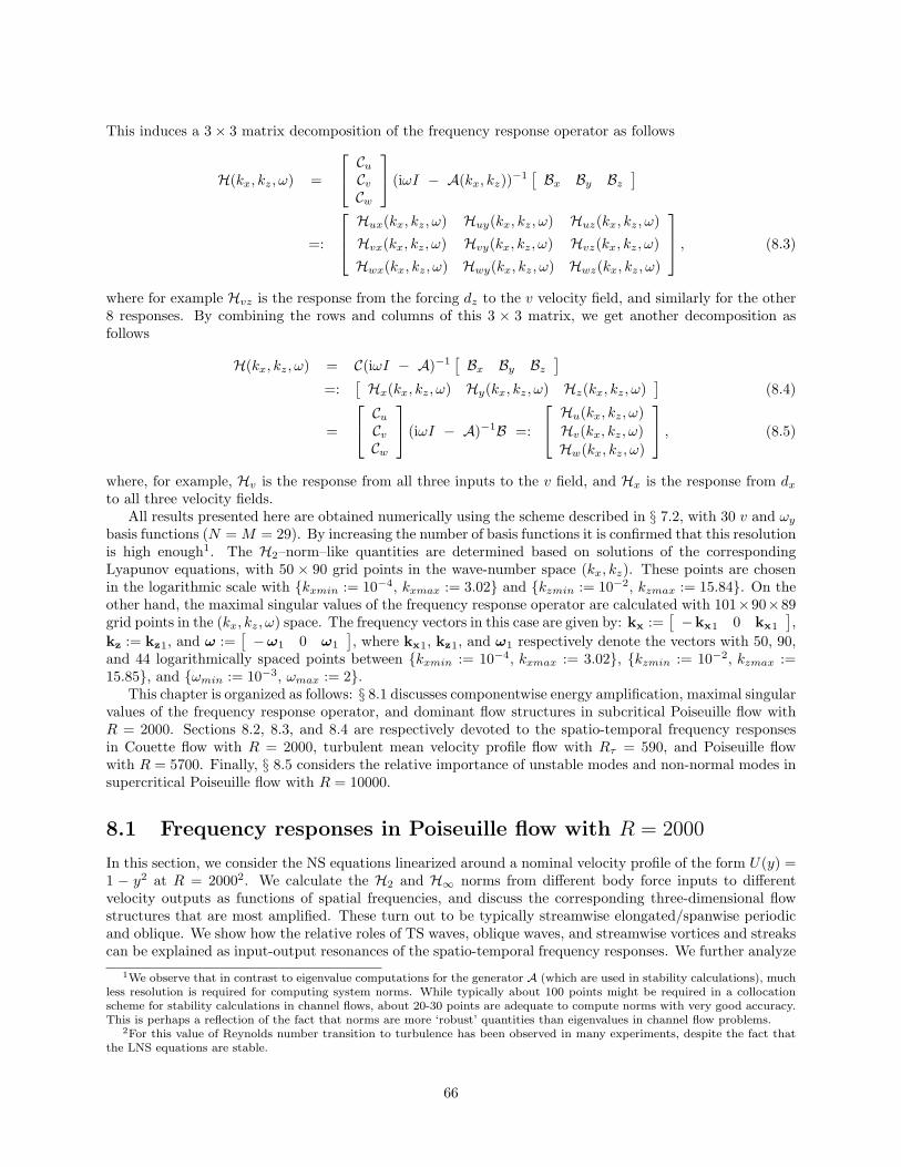
This induces a 3 × 3 matrix decomposition of the frequency response operator as follows
H(kx, kz, ω) =
Cu
CvCw
(iωI − A(kx, kz))−1
[Bx By Bz
]
=:
Hux(kx, kz, ω) Huy(kx, kz, ω) Huz(kx, kz, ω)
Hvx(kx, kz, ω) Hvy(kx, kz, ω) Hvz(kx, kz, ω)
Hwx(kx, kz, ω) Hwy(kx, kz, ω) Hwz(kx, kz, ω)
, (8.3)
where for example Hvz is the response from the forcing dz to the v velocity field, and similarly for the other8 responses. By combining the rows and columns of this 3 × 3 matrix, we get another decomposition asfollows
H(kx, kz, ω) = C(iωI − A)−1[Bx By Bz
]=:
[Hx(kx, kz, ω) Hy(kx, kz, ω) Hz(kx, kz, ω)
](8.4)
=
Cu
CvCw
(iωI − A)−1B =:
Hu(kx, kz, ω)
Hv(kx, kz, ω)Hw(kx, kz, ω)
, (8.5)
where, for example, Hv is the response from all three inputs to the v field, and Hx is the response from dxto all three velocity fields.
All results presented here are obtained numerically using the scheme described in § 7.2, with 30 v and ωybasis functions (N = M = 29). By increasing the number of basis functions it is confirmed that this resolutionis high enough1. The H2–norm–like quantities are determined based on solutions of the correspondingLyapunov equations, with 50 × 90 grid points in the wave-number space (kx, kz). These points are chosenin the logarithmic scale with kxmin := 10−4, kxmax := 3.02 and kzmin := 10−2, kzmax := 15.84. On theother hand, the maximal singular values of the frequency response operator are calculated with 101×90×89grid points in the (kx, kz, ω) space. The frequency vectors in this case are given by: kx :=
[−kx1 0 kx1
],
kz := kz1, and ω :=[−ω1 0 ω1
], where kx1, kz1, and ω1 respectively denote the vectors with 50, 90,
and 44 logarithmically spaced points between kxmin := 10−4, kxmax := 3.02, kzmin := 10−2, kzmax :=15.85, and ωmin := 10−3, ωmax := 2.
This chapter is organized as follows: § 8.1 discusses componentwise energy amplification, maximal singularvalues of the frequency response operator, and dominant flow structures in subcritical Poiseuille flow withR = 2000. Sections 8.2, 8.3, and 8.4 are respectively devoted to the spatio-temporal frequency responsesin Couette flow with R = 2000, turbulent mean velocity profile flow with Rτ = 590, and Poiseuille flowwith R = 5700. Finally, § 8.5 considers the relative importance of unstable modes and non-normal modes insupercritical Poiseuille flow with R = 10000.
8.1 Frequency responses in Poiseuille flow with R = 2000
In this section, we consider the NS equations linearized around a nominal velocity profile of the form U(y) =1 − y2 at R = 20002. We calculate the H2 and H∞ norms from different body force inputs to differentvelocity outputs as functions of spatial frequencies, and discuss the corresponding three-dimensional flowstructures that are most amplified. These turn out to be typically streamwise elongated/spanwise periodicand oblique. We show how the relative roles of TS waves, oblique waves, and streamwise vortices and streakscan be explained as input-output resonances of the spatio-temporal frequency responses. We further analyze
1We observe that in contrast to eigenvalue computations for the generator A (which are used in stability calculations), muchless resolution is required for computing system norms. While typically about 100 points might be required in a collocationscheme for stability calculations in channel flows, about 20-30 points are adequate to compute norms with very good accuracy.This is perhaps a reflection of the fact that norms are more ‘robust’ quantities than eigenvalues in channel flow problems.
2For this value of Reynolds number transition to turbulence has been observed in many experiments, despite the fact thatthe LNS equations are stable.
66

the effectiveness of input field components, and the energy content of u, v, and w. Also, we demonstrate thatthe wall-normal and spanwise forces have much stronger influence on the velocity field than the streamwiseforce, and that the impact of these forces is most powerful on the streamwise velocity component.
8.1.1 Componentwise energy amplification
We first study the frequency responses (as a function of kx and kz) of each of the components (subsystems)of the transfer function (8.3). We do this using the H2 norm, that is
[‖Hrs‖2
2
](kx, kz) :=
12π
∫ ∞
−∞||Hrs(kx, kz, ω)||2HS dω, for r = u, v, w, and s = x, y, z.
From Chapter 2, we recall that the H2 norm has an interesting stochastic interpretation: it quantifies thevariance (energy) amplification of harmonic (in x and z) stochastic (in y and t) disturbances at any givenwave-number pair (kx, kz). In the fluid mechanics literature this measure of input-output amplification isalso referred to as the ensemble average energy density of the statistical steady-state [1].
The (kx, kz)–parameterized H2 norms of all components of the frequency response operator are illustratedin Figure 8.1. Different plots correspond to the different elements of the operator valued matrix on the right-hand side of (8.3). All plots are given in the log–log–linear scale. We make the following observations:
• Input-output amplifications from dy and dz to u attain the largest values. Clearly, both[‖Huy‖2] (kx, kz) and [‖Huz‖2] (kx, kz) have fairly similar shapes with distinctive peaks whose valuesare at least one order of magnitude larger than the peak values of all other quantities shown inFigure 8.1. This illustrates that the wall-normal and spanwise forces have much stronger influence onthe velocity field than the streamwise force, and that the impact of these forces is most powerful onthe streamwise velocity component.
• Different components of frequency response peak at different locations in the (kx, kz)–plane. Hence, the componentwise input-output analysis uncovers several distinct amplification mech-anisms. These mechanisms are responsible for creation of streamwise vortices and streaks (peak valuesat kx ≈ 0, kz ≈ O(1)), oblique waves (peak values at kx ≈ O(1), kz ≈ O(1)), and TS waves (peakvalues at kx ≈ O(1), kz ≈ 0).
• The streamwise elongated structures are most amplified by system’s dynamics, followedby the oblique perturbations, followed by the TS waves. Clearly, there is about an order ofmagnitude difference between the largest peak values taking place at (kx ≈ 0, kz ≈ O(1)) and at(kx ≈ O(1), kz ≈ O(1)). On the other hand, in Poiseuille flow with R = 2000 the oblique waves areapproximately four times more amplified than the least-stable LNS modes (TS waves). However, thisis not to say that the TS waves and especially the oblique waves should be neglected in studies oftransition. Either of them can trigger nonlinear terms in the full NS equations. Moreover, the phaseof these perturbations can play an important role when the flow is connected in feedback with, forexample, a controller for drag reduction.
We note that the importance of the streamwise vortices and streaks was thoroughly studied by [1–5],among others. The fact that the oblique waves often produce the greatest transient amplification wasrecognized by Farrell and Ioannou [6] in the study of the three-dimensional perturbations to viscous constantshear flow that give the largest energy growth on a selected time interval. Also, a Karhunen–Loeve analysis ofa direct numerical simulation of turbulent channel flow at Rτ = 80 revealed the presence of energetic obliquewaves [7]. Oblique wave transition scenario was introduced in [8]. This transition scenario was studiedexperimentally in Poiseuille flow [9], and both experimentally and numerically in boundary layers [10]. Thetransition thresholds in oblique plane channel flow transition were examined in [11], and recently in [12]. Theidentification of the oblique waves as the input-output resonances of the LNS equations illustrates usefulnessof the input-output approach to the analysis of the problem at hand.
67
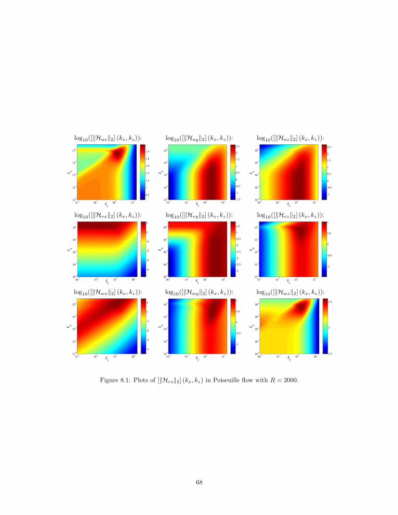
log10([‖Hux‖2] (kx, kz)): log10([‖Huy‖2] (kx, kz)): log10([‖Huz‖2] (kx, kz)):
log10([‖Hvx‖2] (kx, kz)): log10([‖Hvy‖2] (kx, kz)): log10([‖Hvz‖2] (kx, kz)):
log10([‖Hwx‖2] (kx, kz)): log10([‖Hwy‖2] (kx, kz)): log10([‖Hwz‖2] (kx, kz)):
Figure 8.1: Plots of [‖Hrs‖2] (kx, kz) in Poiseuille flow with R = 2000.
68

log10([‖Hx‖2] (kx, kz)): log10([‖Hy‖2] (kx, kz)): log10([‖Hz‖2] (kx, kz)):
Figure 8.2: Plots of [‖Hx‖2] (kx, kz), [‖Hy‖2] (kx, kz), and [‖Hz‖2] (kx, kz), in Poiseuille flow with R = 2000.
Figure 8.2 shows the H2 norms of different components of frequency response operator (8.4), that is
[‖Hs‖2
2
](kx, kz) :=
12π
∫ ∞
−∞||Hs(kx, kz, ω)||2HS dω, for s = x, y, z.
These plots quantify the amplification from inputs in the three spatial directions to the velocity vectorφ =
[u v w
]T . The square additive property of the H2 norm implies that these plots can be obtainedby summing the rows in Figure 8.1. We note that:
• The external excitations applied in the wall-normal and spanwise directions have muchbigger impact on the velocity field than the streamwise direction forcing. The analyticalexplanation for this observation is given in § 9.3, where we show that the energy of three-dimensionalstreamwise constant perturbations in the presence of either dy or dz achieves O(R3) amplification. Onthe other hand, only amplification proportional to the Reynolds number is achievable when externalforce in the streamwise direction is applied, as illustrated in § 9.3.
• Functions [‖Hy‖2] (kx, kz) and [‖Hz‖2] (kx, kz) achieve their largest values at the differentlocations in the (kx, kz)–plane than function [‖Hx‖2] (kx, kz). Clearly, the former two quanti-ties peak at kx = 0 for certain O(1) value of kz. These input-output resonances correspond to thestreamwise vortices and streaks. On the other hand, the latter quantity attains the global maximumat the location where both spatial wave-numbers have O(1) values. We also observe a local peak at thestreamwise wave-number axis in the left plot. This peak is caused by the least-stable modes of A (TSwaves). Even though the presence of the least-stable modes in the left plot is more prominent than inthe middle and right plots, the structures that are more amplified by the system’s dynamics are stillthree-dimensional. These structures correspond to the oblique waves.
Figure 8.3 illustrates the energy content of different velocity components by showing the kx–kz dependenceof the H2 norm of frequency response operator (8.5), that is
[‖Hr‖2
2
](kx, kz) :=
12π
∫ ∞
−∞||Hr(kx, kz, ω)||2HS dω, for r = u, v, w.
These plots quantify the respective amplification from input vector d :=[dx dy dz
]T to velocity pertur-bations u, v, and w. The square additive property of the H2 norm implies that these plots can be obtainedby summing the columns in Figure 8.1. We remark that:
• The energy content of the streamwise velocity is much bigger than the energy content ofthe other two velocity components. The analytical explanation for this observation is given in§ 9.3, where we explicitly show that the variance of three-dimensional streamwise velocity perturbationsat kx = 0 scales as R3. This is in sharp contrast with the amplification that v and w experience. Namely,
69
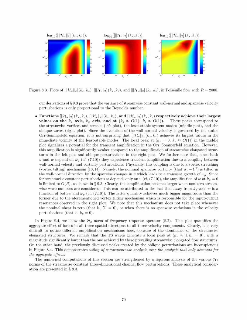
log10([‖Hu‖2] (kx, kz)): log10([‖Hv‖2] (kx, kz)): log10([‖Hw‖2] (kx, kz)):
Figure 8.3: Plots of [‖Hu‖2] (kx, kz), [‖Hv‖2] (kx, kz), and [‖Hw‖2] (kx, kz), in Poiseuille flow with R = 2000.
our derivations of § 9.3 prove that the variance of streamwise constant wall-normal and spanwise velocityperturbations is only proportional to the Reynolds number.
• Functions [‖Hu‖2] (kx, kz), [‖Hv‖2] (kx, kz), and [‖Hw‖2] (kx, kz) respectively achieve their largestvalues on the kz–axis, kx–axis, and at (kx ≈ O(1), kz ≈ O(1)). These peaks correspond tothe streamwise vortices and streaks (left plot), the least-stable system modes (middle plot), and theoblique waves (right plot). Since the evolution of the wall-normal velocity is governed by the stableOrr-Sommerfeld equation, it is not surprising that [‖Hv‖2] (kx, kz) achieves its largest values in theimmediate vicinity of the least-stable modes. The local peak at (kx = 0, kz ≈ O(1)) in the middleplot signalizes a potential for the transient amplification in the Orr–Sommerfeld equation. However,this amplification is significantly weaker compared to the amplification of streamwise elongated struc-tures in the left plot and oblique perturbations in the right plot. We further note that, since bothu and w depend on ωy (cf. (7.10)) they experience transient amplification due to a coupling betweenwall-normal velocity and vorticity perturbations. Physically, this coupling is due to a vortex stretching(vortex tilting) mechanism [13, 14]. Namely, the nominal spanwise vorticity (that is, −U ′) is tilted inthe wall-normal direction by the spanwise changes in v which leads to a transient growth of ωy. Sincefor streamwise constant perturbations w depends only on v (cf. (7.10)), the amplification of w at kx = 0is limited to O(R), as shown in § 9.3. Clearly, this amplification becomes larger when non-zero stream-wise wave-numbers are considered. This can be attributed to the fact that away from kz–axis w is afunction of both v and ωy (cf. (7.10)). The latter quantity achieves much bigger magnitudes than theformer due to the aforementioned vortex tilting mechanism which is responsible for the input-outputresonances observed in the right plot. We note that this mechanism does not take place wheneverthe nominal shear is zero (that is, U ′ = 0), or when there is no spanwise variations in the velocityperturbations (that is, kz = 0).
In Figure 8.4, we show the H2 norm of frequency response operator (8.2). This plot quantifies theaggregate effect of forces in all three spatial directions to all three velocity components. Clearly, it is verydifficult to notice different amplification mechanisms here, because of the dominance of the streamwiseelongated structures. We remark that the TS waves generate a local peak at (kx ≈ 1, kz = 0), with amagnitude significantly lower than the one achieved by these prevailing streamwise elongated flow structures.On the other hand, the previously discussed peaks created by the oblique perturbations are inconspicuousin Figure 8.4. This demonstrates utility of componentwise analysis over the analysis that only accounts forthe aggregate effects.
The numerical computations of this section are strengthened by a rigorous analysis of the various H2
norms of the streamwise constant three-dimensional channel flow perturbations. These analytical consider-ation are presented in § 9.3.
70

log10([‖H‖2] (kx, kz)):
Figure 8.4: Plot of [‖H‖2] (kx, kz) in Poiseuille flow with R = 2000.
10−2
100
102
100
1
2
3
4
kz
kx
log 10
([||H
|| ∞](
k x,kz))
10−2
10−1
100
101
10−4
10−3
10−2
10−1
100
kz
k x
1.99
1.99
3.26
4.12
4.12
Figure 8.5: Plots of [‖H‖∞](kx, kz) in Poiseuille flow with R = 2000.
8.1.2 Maximal singular values
In this subsection, we study the H∞–norm–like quantities of the transfer function (8.3). These quantities areobtained by taking suprema of σmax(H(kx, kz, ω)) over different frequencies. For example, from § 2.2.2 werecall that, the H∞ norm of system (7.18) with a frequency response (8.2) represents a (kx, kz)–parameterizedfunction given by
[‖H‖∞] (kx, kz) := supω
σmax(H(kx, kz, ω)).
Suprema over spatial wave-numbers can be determined in a similar fashion.We remind the reader that [‖H‖∞] (kx, kz) has an interesting physical interpretation: at any pair (kx, kz)
it quantifies the worst case amplification of deterministic inputs. In other words, [‖H‖∞] (kx, kz) represent amaximization of the gain from d to φ over input temporal frequencies and wall-normal shapes at given spatialwave-numbers. The former is obtained by the maximization over ω and the latter by taking a maximumsingular value. Also, from § 2.2.6 we recall that [‖H‖∞] (kx, kz) can be used to asses the stability marginof the LNS system (7.18) at any pair (kx, kz). Namely, the H∞ norm precisely determines the ‘size’ ofunstructured uncertainty that can be used to destabilize the system: the larger [‖H‖∞] (kx, kz) the smallerstability margin of the LNS equations.
Figure 8.5 reveals the dependence of the H∞ norm of system (8.2) on both kx and kz in Poiseuille flowwith R = 2000. The global maximum occurs at (kx = 0, kz ≈ 1.62). Based on contour plots, we also noticea local peak at (kx ≈ 0.0015, kz ≈ 1.62). This local maximum has a value very close to the value of theglobal maximum. Under-damped system modes create a local peak at (kx ≈ 1, kz = 0), with a magnitudesignificantly lower than the magnitude achieved by dominant streamwise constant flow structures.
Figure 8.6 illustrates the maximal singular value plots of the operators H, Hx, Hy, and Hz in Poiseuilleflow with R = 2000. For example, the left plot shows the kx–dependence of supkz,ω σmax(H(kx, kz, ω)) forthese four operators. We make the following observations:
71

10-4
10-3
10-2
10-1
100
101
1
1.5
2
2.5
3
3.5
4
4.5
kx
log 10
(sup
k z,ω σ m
ax(H
(kx,k
z,ω))
)
10-2
10-1
100
101
102
0.5
1
1.5
2
2.5
3
3.5
4
4.5
kz
log 10
(sup
k x,ω σ m
ax(H
(kx,k
z,ω))
)
10-3
10-2
10-1
100
101
1
1.5
2
2.5
3
3.5
4
4.5
ω
log 10
(sup
k x,kz σ m
ax(H
(kx,k
z,ω))
)
Figure 8.6: Maximal singular values of operators H(kx, kz, ω) (solid), Hx(kx, kz, ω) (dash–dot), Hy(kx, kz, ω)(dot), and Hz(kx, kz, ω) (dash) in Poiseuille flow with R = 2000. In all three cases the dependence on theremaining two frequencies is taken away by determining a supremum over them.
• Streamwise elongated effects with large time constants dominate the evolution of thevelocity perturbations. Since all curves in the left and right plots achieve their peak values at(kx = 0, ω = 0), this statement holds irrespective of spatial direction in which external excitationis applied. The results of § 8.1.1 do not contain any information about the temporal evolution ofperturbations due to integration in time. On the other hand, the right plot in Figure 8.6 illustratesprevalence of perturbations that change slowly with time.
• It appears that system acts as a low pass filter in both x and t. When only forcing in thestreamwise direction is applied, the LNS system behaves as a low pass filter in z as well. In this case, thespanwise elongated structures are most amplified by system’s dynamics. However, this amplificationis approximately two orders of magnitude smaller than the amplification achieved in the presence ofeither dy or dz.
• Dominant spanwise length scale is much smaller than the dominant streamwise lengthscale when either dy or dz acts. This is a direct consequence of the fact that the most amplifiedregion of spanwise wave-numbers takes place away from kz = 0, at kz = O(1).
Moreover, we note that even after taking suprema over two frequencies the dominance of streamwiseelongated/spanwise periodic structures with long time constants is still identified using our approach. Thesestructures are ubiquitous in experimental investigations related to transition in both channel and boundarylayer flows [15–18]. This further exemplifies the power of the input-output approach to the analysis of theLNS equations.
8.1.3 Dominant flow structures
The left plot in Figure 8.7 shows the singular values of operator (8.2), arranged in descending order, at thelocation in the frequency space where σmax(H(kx, kz, ω)) achieves global maximum. This plot illustrates theexistence of two strongly amplified perturbation types at (kx = 0, kz = 1.62, ω = 0).
The flow structures corresponding to the two largest singular values of operator H(0, 1.62, 0) are shownin Figure 8.8. The development of streamwise velocity (pseudo-color plots), and stream-function (contourplots) perturbations in the channel’s cross-section is given. These perturbations are streamwise constantand, as such, they do not vary in the direction of the nominal flow. Several comments are in order:
• The most amplified set of perturbations results in pairs of counter rotating streamwisevortices that generate high and low speed streaks symmetric with respect to the channel’scenterline. These perturbations have striking resemblance to the ‘Poiseuille flow symmetric globaloptima’ determined by Butler & Farrell [2] in their analysis of the most energetic initial conditions. Wenote that these perturbations experience energy growth that is approximately twice smaller than theenergy growth of ‘antisymmetric global optima’ [2]. As remarked by Butler & Farrell [2], the exper-imental conditions, such as surface roughness or level of background noise, ‘may select perturbations
72

0 5 10 15 20 25 30 35 400
0.5
1
1.5
2
2.5
3
3.5
4
4.5
mode number
log 10
(σ(H
(0,1
.62,
0)))
0 5 10 15 20 25 30 35 400
0.5
1
1.5
2
2.5
3
3.5
4
4.5
mode number
log 10
(σ(H
(0.0
1,1.
67,-
0.00
66))
)
0 5 10 15 20 25 30 35 400
0.5
1
1.5
2
2.5
3
3.5
4
mode number
log 10
(σ(H
(0.1
,2.1
2,-0
.066
)))
Figure 8.7: Singular values of operator (8.2) at: (kx = 0, kz = 1.62, ω = 0) (left), (kx = 0.01, kz = 1.67, ω =−0.0066) (middle), and (kx = 0.1, kz = 2.12, ω = −0.066) (right), in Poiseuille flow with R = 2000.
Figure 8.8: Streamwise velocity (pseudo-color plots), and stream-function (contour plots) perturbation devel-opment for largest singular value (left) and second largest singular value (right) of operator (8.2) at (kx = 0,kz = 1.62, ω = 0) (location where the global maximum of σmax(H(kx, kz, ω)) takes place), in Poiseuille flowwith R = 2000. Red color represents high speed streaks, and blue color represents low speed streaks.
that grow robustly but not necessarily optimally3’. Our results indicate that symmetric perturbationsare most amplified by the system’s dynamics in the presence of unstructured spatially distributed andtemporally varying external excitations.
• There exists no general relationship between transient growth and input-output analyses.As already mentioned, the former focuses on the search for initial perturbations that gain the mostenergy on a certain time interval. On the other hand, the latter studies the LNS system in thepresence of body forces. One of the goals of the input-output analysis may be determination of flowstructures that are strongly amplified by the externally excited LNS dynamics. The results presentedhere establish that, in Poiseuille flow, the transient growth global optima do not correspond to theflow perturbations most amplified by the forced LNS equations. In § 8.2, we will illustrate that thisis also the situation in Couette flow. Namely, it turns out that the dominant input-output resonancesin Couette flow are streamwise constant. On the other hand, the flow perturbations with very slowstreamwise variations and kz ≈ 1.60 have the strongest transient growth potential [2, 4].
• The second set of strongly amplified perturbations results in four streamwise vorticesoccupying the channel width. These counter-rotating vortices generate strong high (low) speedstreaks in the near wall regions and a slightly weaker low (high) speed streak that fills the middle ofthe channel.
3Word optimal is used to denote initial perturbations that are capable of most energetic transient growth [2].
73

isosurface plots of u: isosurface plots of u and ωx:
Figure 8.9: Streamwise velocity and vorticity perturbation development for largest singular value of operatorH at (kx = 0.01, kz = 1.67, ω = −0.0066), in Poiseuille flow with R = 2000. High (low) velocity and vorticityregions are respectively represented by red and yellow (green and blue) colors. Isosurfaces of u and ωx arerespectively taken at ±0.5 and ±0.1.
The results shown in Figures 8.5 and 8.6 indicate that σmax(H(kx, kz, ω)) has a fairly uniform value in theregion of kz’s where this quantity peaks so long as (approximately) |kx| < 0.1 and |ω| < 0.1. This is furtherillustrated in the middle and right plots in Figure 8.7, where we respectively show the singular values of Hat (kx = 0.01, kz = 1.67, ω = −0.0066), and (kx = 0.1, kz = 2.12, ω = −0.066). We still observe presence oftwo strongly amplified perturbations.
The streamwise velocity and vorticity perturbation developments for these two cases are shown in Fig-ures 8.9, 8.10, and 8.11. We remark that:
• The plots are characterized by the alternating regions of high and low velocities thatare elongated in the streamwise directions. Some of the plots have the form of downstreamoriented arrowhead-shaped structures. This rather characteristic shape is observed experimentally inlaminar-turbulent transition studies in both channel [15–17] and boundary layer flows [18,19].
• The velocity (vorticity) perturbations develop symmetrically (antisymmetrically) aboutthe channel’s centerline.
• The vortices are positioned between the high and low velocity regions.
• There is a large concentration of arrays of counter rotating streamwise vortices in thevicinity of the lower and upper walls. These streamwise vortices transport low-velocity fluid awayfrom the walls towards the channel centerline and redistribute it in the spanwise direction.
• Experimental and DNS results are characterized by the interaction of different modesrather than by a dominance of one particular mode. Thus, the real flow is going to be muchmore complicated than the structures shown here. Nevertheless, the performed analysis serves as anindication of structures that can be expected to be seen in both experimental and numerical transitioninvestigations. In Chapter 10, we will illustrate that the results presented here exhibit some qualitativesimilarities with the spatio-temporal impulse responses of the LNS equations.
To illustrate that most results of this section represent universal properties of the wall-bounded shearflows rather than just distinctive features of the plane Poiseuille flow, in § 8.2 and § 8.3, we respectivelydiscuss frequency responses of the plane Couette flow with R = 2000 and turbulent mean velocity profileflow with Rτ = 590.
74

isosurface plots of u: isosurface plots of u and ωx:
Figure 8.10: Streamwise velocity and vorticity perturbation development for second largest singular valueof operator H at (kx = 0.01, kz = 1.67, ω = −0.0066), in Poiseuille flow with R = 2000. High (low) velocityand vorticity regions are respectively represented by red and yellow (green and blue) colors. Isosurfaces ofboth u and ωx are taken at ±0.5.
Figure 8.11: Streamwise velocity perturbation development for largest singular value (first row) and secondlargest singular value (second row) of operator H at (kx = 0.1, kz = 2.12, ω = −0.066), in Poiseuille flowwith R = 2000. High speed streaks are represented by red color, and low speed streaks are represented bygreen color. Isosurfaces are taken at ±0.5.
75

8.2 Frequency responses in Couette flow with R = 2000
In this section, we present different portions of the spatio-temporal frequency responses for the NS equationslinearized around a nominal velocity profile of the form U(y) = y at R = 2000. We compare the resultspresented here with the results presented in § 8.1 and find many qualitative similarities.
Figure 8.12 illustrates the effectiveness of input field components by showing the (kx, kz)–dependence ofthe H2 norm for all subsystems in (8.4). As in Poiseuille flow, excitations in the spanwise and wall-normaldirections have much bigger influence on flow perturbations than the streamwise excitation. Furthermore,the peaks in the middle and right plots take place on the kz–axis, whereas the peak in the left plot is movedto the location where both kx = 0 and kz = 0. The absence of the streamwise forcing in the equation thatgoverns the evolution of the wall-normal velocity at kx = 0 prevents large amplification in the latter case (see§ 9.3 for analytical explanation). This amplification becomes bigger for non-zero values of kx, but clearly, itnever reaches values achieved by [‖Hy‖2] (kx, kz) and [‖Hz‖2] (kx, kz).
log10([‖Hx‖2] (kx, kz)): log10([‖Hy‖2] (kx, kz)): log10([‖Hz‖2] (kx, kz)):
Figure 8.12: Plots of [‖Hx‖2] (kx, kz), [‖Hy‖2] (kx, kz), and [‖Hz‖2] (kx, kz), in Couette flow with R = 2000.
Energy content of streamwise, wall-normal, and spanwise velocity components in Couette flow withR = 2000 is shown in Figure 8.13. By comparing these plots with their Poiseuille flow counterparts weconclude that they have fairly similar features. Furthermore, as in § 8.1, we note the dominance of thestreamwise velocity perturbations.
log10([‖Hu‖2] (kx, kz)): log10([‖Hv‖2] (kx, kz)): log10([‖Hw‖2] (kx, kz)):
Figure 8.13: Plots of [‖Hu‖2] (kx, kz), [‖Hv‖2] (kx, kz), and [‖Hw‖2] (kx, kz), in Couette flow with R = 2000.
Our computations show that the largest input-output gains in Couette flow are achieved at (kx = 0, kz ≈O(1)). This may seem to be at odds with [2,4], where it was established that, in Couette flow, the spanwiseperiodic perturbations with very slow streamwise variations generate the largest transient growth. We remarkagain that there is no general relationship between transient growth and input-output analyses (see § 8.1.3for additional discussions). In view of this, both these results are correct and they are not in disagreementwith each other. Not only does our analysis uncover the streamwise constant/spanwise periodic structuresas the most amplified input-output resonances, but it also reveals that the spanwise periodic structures with
76

slow streamwise variations are strongly amplified by the LNS dynamics. Thus, in experimental or numericalinvestigations one should expect to observe both these effects.
We note that the spectral analysis of Couette and Poiseuille flows indicates that these two flows are quitedifferent. Namely, the former is stable for all values of R [20], and the latter losses stability when R achievesvalues greater than 5772 [21]. However, according to the results of § 8.1 and § 8.2 these two flows have fairlysimilar qualitative features when analyzed from an input-output point of view.
8.3 Frequency responses in turbulent mean velocity profile flowwith Rτ = 590
In this section, we study the frequency responses for the flow that satisfies the NS equations linearized aroundturbulent mean velocity profile with Rτ = 590. This velocity profile is shown in Figure 8.14, and it wasobtained by direct numerical simulations of the channel flow at Rτ = 590 [22]. This section illustrates thatour methodology can be applied to study input-output properties of the system linearized around a velocityprofile that is not a steady-state solution of the NS equations. Also, we compare the results presented herewith the results obtained in subcritical Poiseuille (cf. § 8.1) and Couette (cf. § 8.2) flows with R = 2000.
-1 -0.5 0 0.5 10
5
10
15
20
y
U
Figure 8.14: Channel flow turbulent mean velocity profile with Rτ = 590.
The (kx, kz)–parameterized H2 norms of each component of operators (8.4) and (8.5) are respectivelyshown in Figures 8.15 and 8.16. Qualitatively, these plots resemble their analogues of § 8.1 and § 8.2. Thestrongly amplified resonances still have long streamwise length scales and certain spanwise periodicity.
Therefore, the frequency domain input-output analysis reveals that all channel flows with a streamwisedirection mean velocity profile that depends only on the wall-normal coordinate are almost alike. This isan important discovery which, for example, indicates that the perturbations around laminar and turbulentchannel flows should act in a similar way. However, the interpretation for these two cases is different. Whilethe laminar flow perturbations initiate transition and consequently lead to turbulence, their turbulent flowcounterparts are primarily responsible for maintenance of the turbulent state. Regardless of the interpre-tation, our results underscore the importance of non-modal effects in both transitional and fully turbulentchannel flows.
8.4 Frequency responses in Poiseuille flow with R = 5700
In this section, we study the frequency responses in subcritical Poiseuille flow with R = 5700. We considerthis problem for two reasons. First, we want to identify the dominant input-output resonances in the flowthat is about to become unstable if the Reynolds number is increased by less than 1.25% (critical value ofReynolds number is approximately equal to 5772 [21]). Second, in § 8.5 we will compare results presentedhere with the results obtained in supercritical Poiseuille flow with R = 10000 in the presence of exponentiallydiscounted input and output signals. Our main conclusions are:
• The dominant input-output resonances are still streamwise vortices and streaks.
77
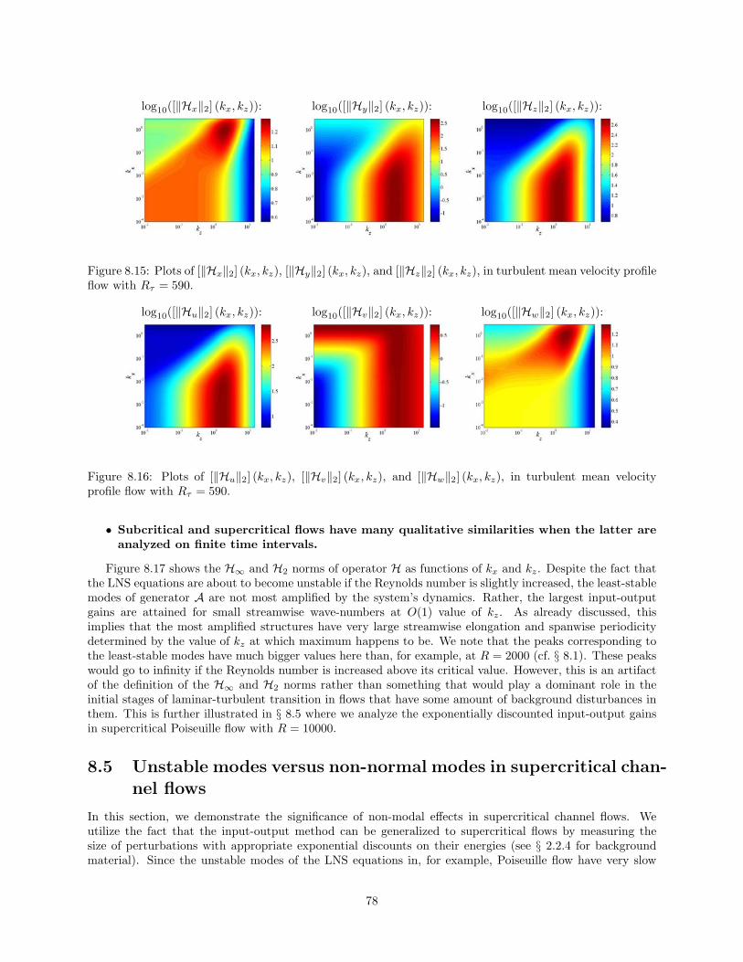
log10([‖Hx‖2] (kx, kz)): log10([‖Hy‖2] (kx, kz)): log10([‖Hz‖2] (kx, kz)):
Figure 8.15: Plots of [‖Hx‖2] (kx, kz), [‖Hy‖2] (kx, kz), and [‖Hz‖2] (kx, kz), in turbulent mean velocity profileflow with Rτ = 590.
log10([‖Hu‖2] (kx, kz)): log10([‖Hv‖2] (kx, kz)): log10([‖Hw‖2] (kx, kz)):
Figure 8.16: Plots of [‖Hu‖2] (kx, kz), [‖Hv‖2] (kx, kz), and [‖Hw‖2] (kx, kz), in turbulent mean velocityprofile flow with Rτ = 590.
• Subcritical and supercritical flows have many qualitative similarities when the latter areanalyzed on finite time intervals.
Figure 8.17 shows the H∞ and H2 norms of operator H as functions of kx and kz. Despite the fact thatthe LNS equations are about to become unstable if the Reynolds number is slightly increased, the least-stablemodes of generator A are not most amplified by the system’s dynamics. Rather, the largest input-outputgains are attained for small streamwise wave-numbers at O(1) value of kz. As already discussed, thisimplies that the most amplified structures have very large streamwise elongation and spanwise periodicitydetermined by the value of kz at which maximum happens to be. We note that the peaks corresponding tothe least-stable modes have much bigger values here than, for example, at R = 2000 (cf. § 8.1). These peakswould go to infinity if the Reynolds number is increased above its critical value. However, this is an artifactof the definition of the H∞ and H2 norms rather than something that would play a dominant role in theinitial stages of laminar-turbulent transition in flows that have some amount of background disturbances inthem. This is further illustrated in § 8.5 where we analyze the exponentially discounted input-output gainsin supercritical Poiseuille flow with R = 10000.
8.5 Unstable modes versus non-normal modes in supercritical chan-nel flows
In this section, we demonstrate the significance of non-modal effects in supercritical channel flows. Weutilize the fact that the input-output method can be generalized to supercritical flows by measuring thesize of perturbations with appropriate exponential discounts on their energies (see § 2.2.4 for backgroundmaterial). Since the unstable modes of the LNS equations in, for example, Poiseuille flow have very slow
78
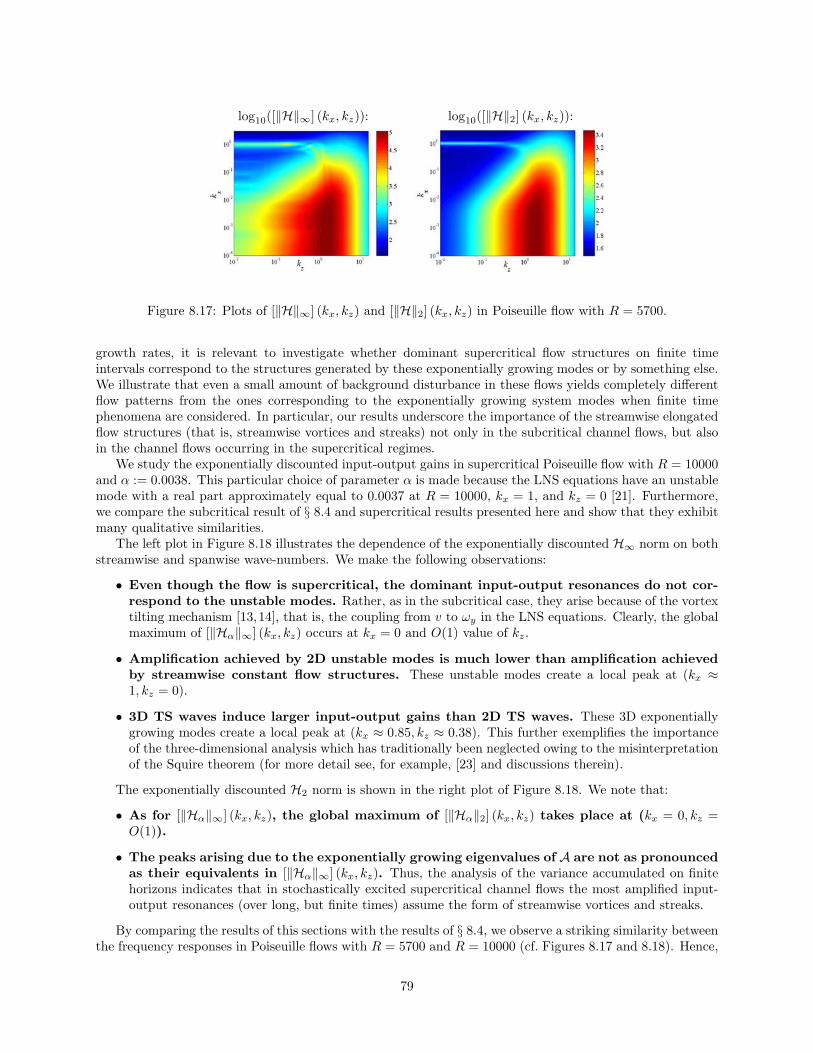
log10([‖H‖∞] (kx, kz)): log10([‖H‖2] (kx, kz)):
Figure 8.17: Plots of [‖H‖∞] (kx, kz) and [‖H‖2] (kx, kz) in Poiseuille flow with R = 5700.
growth rates, it is relevant to investigate whether dominant supercritical flow structures on finite timeintervals correspond to the structures generated by these exponentially growing modes or by something else.We illustrate that even a small amount of background disturbance in these flows yields completely differentflow patterns from the ones corresponding to the exponentially growing system modes when finite timephenomena are considered. In particular, our results underscore the importance of the streamwise elongatedflow structures (that is, streamwise vortices and streaks) not only in the subcritical channel flows, but alsoin the channel flows occurring in the supercritical regimes.
We study the exponentially discounted input-output gains in supercritical Poiseuille flow with R = 10000and α := 0.0038. This particular choice of parameter α is made because the LNS equations have an unstablemode with a real part approximately equal to 0.0037 at R = 10000, kx = 1, and kz = 0 [21]. Furthermore,we compare the subcritical result of § 8.4 and supercritical results presented here and show that they exhibitmany qualitative similarities.
The left plot in Figure 8.18 illustrates the dependence of the exponentially discounted H∞ norm on bothstreamwise and spanwise wave-numbers. We make the following observations:
• Even though the flow is supercritical, the dominant input-output resonances do not cor-respond to the unstable modes. Rather, as in the subcritical case, they arise because of the vortextilting mechanism [13,14], that is, the coupling from v to ωy in the LNS equations. Clearly, the globalmaximum of [‖Hα‖∞] (kx, kz) occurs at kx = 0 and O(1) value of kz.
• Amplification achieved by 2D unstable modes is much lower than amplification achievedby streamwise constant flow structures. These unstable modes create a local peak at (kx ≈1, kz = 0).
• 3D TS waves induce larger input-output gains than 2D TS waves. These 3D exponentiallygrowing modes create a local peak at (kx ≈ 0.85, kz ≈ 0.38). This further exemplifies the importanceof the three-dimensional analysis which has traditionally been neglected owing to the misinterpretationof the Squire theorem (for more detail see, for example, [23] and discussions therein).
The exponentially discounted H2 norm is shown in the right plot of Figure 8.18. We note that:
• As for [‖Hα‖∞] (kx, kz), the global maximum of [‖Hα‖2] (kx, kz) takes place at (kx = 0, kz =O(1)).
• The peaks arising due to the exponentially growing eigenvalues of A are not as pronouncedas their equivalents in [‖Hα‖∞] (kx, kz). Thus, the analysis of the variance accumulated on finitehorizons indicates that in stochastically excited supercritical channel flows the most amplified input-output resonances (over long, but finite times) assume the form of streamwise vortices and streaks.
By comparing the results of this sections with the results of § 8.4, we observe a striking similarity betweenthe frequency responses in Poiseuille flows with R = 5700 and R = 10000 (cf. Figures 8.17 and 8.18). Hence,
79

log10([‖Hα‖∞] (kx, kz)): log10([‖Hα‖2] (kx, kz)):
Figure 8.18: Plots of [‖Hα‖∞] (kx, kz) and [‖Hα‖2] (kx, kz) in Poiseuille flow with R = 10000 and α = 0.0038.
we conclude that subcritical and supercritical channel flows are qualitatively similar to each other providedthat the latter are analyzed on finite time intervals.
The results of this section illustrate that even a small amount of external excitation in supercriticalflows yields completely different flow patterns from the ones corresponding to the exponentially growingsystem modes when finite time phenomena are considered. In particular, we have established importanceof the streamwise vortices and streaks in both subcritical and supercritical channel flows. We have alsodemonstrated the striking similarity between the supercritical and subcritical flows when the former areanalyzed using the exponentially discounted system gains. The fact that the frequency response peaksproduced by the TS waves (especially the three-dimensional ones) achieve much higher magnitudes than thecorresponding peaks in subcritical channel flows at moderate Reynolds numbers (e.g. R = 2000) suggests thatmost turbulent flows probably have both instabilities and high amplification of background disturbances.
8.6 Summary
We consider the NS equations linearized around some parallel channel flow U(y) (e.g., Poiseuille, Couette,and turbulent mean velocity profile), in the presence of spatially distributed and temporally varying three-dimensional body forces viewed as inputs. We carry out an input-output analysis in the frequency domainto investigate the dependence of different velocity ‘outputs’ (u, v, w) on the different body force ‘inputs’(dx, dy, dz). We show how the relative roles of TS waves, oblique waves, and streamwise vortices and streakscan be explained as input-output resonances of the spatio-temporal frequency responses.
The effects of the inputs (dx, dy, dz) on velocity fields are dependent on various parameters. We carryout a detailed study of these effects by quantifying them using system norms (also known as gains oramplifications), namely the so-called H∞ and H2 norms. We investigate the dependence of these normson spatial frequencies, as well as the Reynolds number R. This frequency response analysis yields severalconclusions, one of which is the dominance of streamwise elongated–spanwise periodic (kx ≈ 0, kz ≈ O(1))and oblique (kx ≈ O(1), kz ≈ O(1)) effects. We also perform a detailed analysis of the effect of individualinputs on individual outputs. It turns out that the spanwise and wall-normal forces have the strongestinfluence on the velocity field. In particular, the impact of these forces is most powerful on the streamwisevelocity component. Also, we calculate system norms as functions of spatial frequencies, and discuss thecorresponding three-dimensional flow structures that are most amplified. These turn out to be typicallystreamwise elongated–spanwise periodic and sometimes oblique, which corresponds to structures commonlyobserved in experimental studies and fully nonlinear initial value simulations in channel flows.
The significance of non-modal effects in supercritical channel flows is also demonstrated. This is done byanalyzing the LNS equations from an input-output point of view in the presence of exponentially discountedinput and output signals. From a physical perspective this type of analysis amounts to accounting for thefinite time phenomena rather than the asymptotic phenomena of infinite time limits. In particular, ourresults underscore the importance of the streamwise elongated flow effects not only in the subcritical channel
80

flows, but also in the channel flows taking place in the supercritical regimes.It is quite compelling to argue that long-but-finite time analysis is relevant when considering linearized
models. These models are not expected to be valid for infinite time in any case, as when perturbations grow,the linearized dynamics are altered. In the supercritical channel flow case, we see that the main features ofthe model (i.e., the modes contributing the most to perturbation energy) are very dependent on whether wetake an infinite time limit or a large-but-finite time limit. The latter is arguably the more reasonable of thetwo, and when viewed this way, we have shown that aside from the energy of the perturbation, the spectralcontent of subcritical and supercritical channel flows is qualitatively very similar.
81

Bibliography
[1] B. F. Farrell and P. J. Ioannou, “Stochastic forcing of the linearized Navier-Stokes equations,” Physicsof Fluids A, vol. 5, no. 11, pp. 2600–2609, 1993.
[2] K. M. Butler and B. F. Farrell, “Three-dimensional optimal perturbations in viscous shear flow,” Physicsof Fluids A, vol. 4, p. 1637, 1992.
[3] S. C. Reddy and D. S. Henningson, “Energy growth in viscous channel flows,” J. Fluid Mech., vol. 252,pp. 209–238, 1993.
[4] L. N. Trefethen, A. E. Trefethen, S. C. Reddy, and T. A. Driscoll, “Hydrodynamic stability withouteigenvalues,” Science, vol. 261, pp. 578–584, 1993.
[5] B. Bamieh and M. Dahleh, “Energy amplification in channel flows with stochastic excitation,” Physicsof Fluids, vol. 13, no. 11, pp. 3258–3269, 2001.
[6] B. F. Farrell and P. J. Ioannou, “Optimal excitation of three-dimensional perturbations in viscousconstant shear flow,” Physics of Fluids A, vol. 5, no. 6, pp. 1390–1400, 1993.
[7] L. Sirovich, K. S. Ball, and L. R. Keefe, “Plane waves and structures in turbulent channel flow,” Physicsof Fluids A, vol. 2, pp. 2217–2226, 1990.
[8] P. J. Schmid and D. S. Henningson, “A new mechanism for rapid transition involving a pair of obliquewaves,” Physics of Fluids A, vol. 4, no. 9, pp. 1986–1989, 1992.
[9] P. A. Elofsson and P. H. Alfredsson, “An experimental study of oblique transition in plane Poiseuilleflow,” J. Fluid Mech., vol. 358, pp. 177–202, 1998.
[10] S. Berlin, M. Wiegel, and D. S. Henningson, “Numerical and experimental investigations of obliqueboundary layer transition,” J. Fluid Mech., vol. 393, pp. 23–57, 1999.
[11] S. C. Reddy, P. J. Schmid, J. S. Baggett, and D. S. Henningson, “On stability of streamwise streaksand transition tresholds in plane channel flows,” J. Fluid Mech., vol. 365, pp. 269–303, 1998.
[12] S. J. Chapman, “Subcritical transition in channel flows,” J. Fluid Mech., vol. 451, pp. 35–97, 2002.
[13] M. T. Landahl, “Wave breakdown and turbulence,” SIAM J. Appl. Math., vol. 28, pp. 735–756, 1975.
[14] ——, “A note on an algebraic instability of inviscid parallel shear flows,” J. Fluid Mech., vol. 98, pp.243–251, 1980.
[15] D. R. Carlson, S. E. Widnall, and M. F. Peeters, “A flow-visualization study of transition in planePoiseuille flow,” J. Fluid Mech., vol. 121, pp. 487–505, 1982.
[16] F. Alavyoon, D. S. Henningson, and P. H. Alfredsson, “Turbulent spots in plane Poiseuille flow - flowvisualization,” Physics of Fluids, vol. 29, no. 4, pp. 1328–1331, 1986.
[17] B. G. B. Klingmann, “On transition due to three-dimensional disturbances in plane Poiseuille flow,” J.Fluid Mech., vol. 240, pp. 167–195, 1992.
82

[18] M. Matsubara and P. H. Alfredsson, “Disturbance growth in boundary layers subjected to free-streamturbulence,” J. Fluid Mech., vol. 430, pp. 149–168, 2001.
[19] F. W. Chambers and A. S. W. Thomas, “Turbulent spots, wave packets, and growth,” Physics of Fluids,vol. 26, no. 5, pp. 1160–1162, 1983.
[20] V. A. Romanov, “Stability of plane-parallel Couette flow,” Funct. Anal. Applics., vol. 7, pp. 137–146,1973.
[21] S. A. Orszag, “Accurate solution of the Orr-Sommerfeld equation,” J. Fluid Mech., vol. 50, pp. 689–703,1971.
[22] R. D. Moser, J. Kim, and N. N. Mansour, “DNS of turbulent channel flow up to Reτ = 590,” Physicsof Fluids, vol. 11, no. 4, pp. 943–945, 1999.
[23] P. J. Schmid and D. S. Henningson, Stability and Transition in Shear Flows. New York: Springer-Verlag, 2001.
83
Chapter 9
The cross sectional 2D/3C model:analytical results
In this chapter, we study the forced LNS equations for streamwise constant three-dimensional perturba-tions. In this special case, the model for velocity perturbations is usually referred to as the two-dimensional,three component (2D/3C) model [1]. The motivation for analysis of this particular model is twofold. First,from numerical computations presented in Chapter 8, one observes that the streamwise constant perturba-tions experience utmost amplification rates. Second, this model is amenable to a thorough analysis whichclarifies the relative strengths of amplification mechanisms from various forcing directions to velocity fieldcomponents, as well as their dependence on the Reynolds number.
The governing dynamics of streamwise constant 3D perturbations are given by setting kx = 0 in (7.18)which yields
∂t
[ψ1
ψ2
]=
[1RL 0
Cp 1RS
] [ψ1
ψ2
]+
[0 By1 Bz1
Bx2 0 0
] dxdydz
, (9.1a)
uvw
=
0 Cu2
Cv1 0Cw1 0
[ ψ1
ψ2
], (9.1b)
withL := ∆−1∆2, S := ∆, Cp := −ikzU ′(y),
Bx2 := ikz, By1 := −k2z∆
−1, Bz1 := −ikz∆−1∂y,
Cu2 := − ikz, Cv1 := I, Cw1 :=
ikz∂y.
These equations are parameterized by two important parameters: the spanwise wave number kz, and theReynolds number R. The wall-normal velocity and vorticity fields are in this chapter respectively denotedby ψ1(y, t, kz) and ψ2(y, t, kz), with the boundary conditions
ψ1(±1, t, kz) = ∂yψ1(±1, t, kz) = ψ2(±1, t, kz) = 0.
We note that the lower-block-triangular generator in (9.1a) is exponentially stable for any finite R and anyparallel flow U(y). This follows from § 7.1.3, where the spectral analysis of the Reynolds number/nominal-velocity independent, normalized Squire and Orr-Sommerfeld operators S and L was performed. Thus, theexpressions for input-output gains that we derive in this chapter are valid for all Reynolds numbers and allnominal velocity profiles U(y).
Our presentation is organized as follows: in § 9.1 we determine the explicit dependence of singular valuesfor each subsystem in (8.3) on the Reynolds number. These relationships are utilized to show how the
84

Hilbert–Schmidt (§ 9.2), H∞ and H2 (§ 9.3) norms scale with R for each of the components of the frequencyresponse (8.3). Furthermore, the square additive property of the Hilbert–Schmidt and H2 norms is used toquantify:
• Amplification from inputs in different spatial directions (dx, dy, dz) to the velocity vectorφ.
• Energy content of different velocity components (u, v, w).
• Aggregate effect of forces in all three spatial directions d to all three velocity componentsφ.
We reinforce the numerical computations of Chapter 8 by explicit analytical derivations to demonstrate that:
• The spanwise and wall-normal forces are much more influential on flow perturbationsthan the streamwise force.
• The impact of these forces is most powerful on the streamwise velocity.
In § 9.4, we study the effectiveness of the near-wall inputs for streamwise constant three dimensional per-turbations. We analytically establish that:
• For near-wall inputs, the spanwise forcing has, by far, the biggest impact on the evolutionof the velocity field components.
These facts were recently observed in experimental and numerical studies of flow control using the Lorentzforce [2–6]. In § 9.5, we employ the procedure developed in Chapter 3 to explicitly determine the Hilbert–Schmidt norms of each element in (8.3) as functions of spanwise wave-number and the appropriately scaledtemporal frequency. In § 9.6, we perform a detailed analysis to show how the H2 norms of different subsystemsdepend on kz for both ‘unstructured’ and ‘structured’ external excitations. This is done by employing theformula derived in § 3.2.2 to determine operator traces of the solutions of the corresponding Lyapunovequations. We close our presentation in § 9.7 with some concluding remarks.
9.1 Dependence of singular values on the Reynolds number
We first study the dependence of singular values on the Reynolds number for each of the components of thetransfer function (8.3). As illustrated in Chapter 2, singular values of operators that map external excitationsto the relevant physical quantities (in this case, velocity field components) can be used to quantify differentmeasures of input amplification by system’s dynamics (e.g., Hilbert–Schmidt, H2, and H∞ norms). Weanalytically establish that the singular values of frequency response operators from both spanwise and wall-normal forcing to streamwise velocity scale as R2, while the singular values of all other components in (8.3)scale at most as R. We also analyze the maximal singular values of each of the components in (8.3) asfunctions of kz and the appropriately scaled temporal frequency.
Application of the temporal Fourier transform allows us to represent system (9.1) in terms of its blockdiagram shown in Figure 9.1 with Ω := ωR. We note that the same temporal scaling was previously employedby Gustavsson [7] in his undertaking to determine the transient growth of the wall-normal vorticity. Fromthis block diagram it follows that operator H(ω, kz, R) that maps
[dx dy dz
]T into[u v w
]T canbe expressed as
uvw
=
Hux(ω, kz, R) Huy(ω, kz, R) Huz(ω, kz, R)
Hvx(ω, kz, R) Hvy(ω, kz, R) Hvz(ω, kz, R)
Hwx(ω, kz, R) Hwy(ω, kz, R) Hwz(ω, kz, R)
dxdydz
:=
RHux(Ω, kz) R2Huy(Ω, kz) R2Huz(Ω, kz)
0 RHvy(Ω, kz) RHvz(Ω, kz)0 RHwy(Ω, kz) RHwz(Ω, kz)
dxdydz
,
(9.2)
85

dy By1 R(iΩI − L)−1
ψ1 − ikzU ′ R(iΩI − S)−1 ψ2 Cu2
u
dx Bx2
dz Bz1
Cv1 v
Cw1w
Figure 9.1: Block diagram of the streamwise constant LNS system (9.1) with Ω := ωR.
whereHux(Ω, kz) := Cu2(iΩI − S)−1Bx2,Huy(Ω, kz) := Cu2(iΩI − S)−1Cp(iΩI − L)−1By1,Huz(Ω, kz) := Cu2(iΩI − S)−1Cp(iΩI − L)−1Bz1,Hrs(Ω, kz) := Cr1(iΩI − L)−1Bs1, r = v, w; s = y, z,
represent the Reynolds number independent operators parameterized only by Ω and kz. Thus, for thestreamwise constant perturbations the frequency responses from dy and dz to u scale as R2, whereas theresponses from all other inputs to other velocity outputs scale linearly with R. In particular, at kx = 0 thestreamwise forcing does not influence the wall-normal and the spanwise velocity components. It is noteworthythat the coupling term Cp := −ikzU ′ is crucial for providing this R2–scaling. Namely, one can observe fromFigure 9.1 that in the absence of shear or spanwise variations in the wall-normal velocity perturbation allcomponents of operator H(0, kz, ω) in (8.3) are at most proportional to R. This further exemplifies theimportance of the vortex stretching mechanism [8] in the wall-bounded shear flows. We remark that thenumerical experiments of [9] indicated that without the coupling from v to ωy the near-wall turbulencedecays in a fully turbulent channel flow.
The following theorem follows directly from (9.2) and the fact that each operator in (9.2) is compact.
Theorem 6 For any streamwise constant channel flow with nominal velocity U(y), the singular values ofoperators Hrs(ω, kz, R) that map ds into r, r = u, v, w; s = x, y, z, are given by
σux,n(ω, kz, R) σuy,n(ω, kz, R) σuz,n(ω, kz, R)
σvx,n(ω, kz, R) σvy,n(ω, kz, R) σvz,n(ω, kz, R)
σwx,n(ω, kz, R) σwy,n(ω, kz, R) σwz,n(ω, kz, R)
=
ςux,n(Ω, kz)R ςuy,n(Ω, kz)R2 ςuz,n(Ω, kz)R2
0 ςvy,n(Ω, kz)R ςvz,n(Ω, kz)R
0 ςwy,n(Ω, kz)R ςwz,n(Ω, kz)R
,
(9.3)
where σrs,n(ω, kz, R) and ςrs,n(Ω, kz) respectively denote the n-th singular values of operators Hrs(ω, kz, R)and Hrs(Ω, kz), with Ω := ωR and n ∈ N.
Several remarks are in order.
Remark 1 For the streamwise constant perturbations, the singular values of the frequency response operatorsfrom the forces in the wall-normal and the spanwise directions to the streamwise velocity scale as R2. In allother cases they scale as R. In particular, at kx = 0 the streamwise forcing does not influence the wall-normaland the spanwise velocity components. This illustrates the dominance of the streamwise velocity perturbationsand the forces in the remaining two spatial directions in high Reynolds number channel flows.
86

Remark 2 The expressions for the terms that multiply R on the right-hand side of (9.3) are the same for allchannel flows, because these terms depend only on nominal-velocity independent operators L and S. On theother hand, the expressions for ςuy,n(Ω, kz) and ςuz,n(Ω, kz) depend on the coupling operator Cp := −ikzU ′(y),and therefore these singular values are nominal-velocity dependent.
Remark 3 Functions ςrs,n(Ω, kz), for every n ∈ N and every r = u, v, w; s = x, y, z, depend only ontwo parameters: the spanwise wave number, and the product between temporal frequency ω and the Reynoldsnumber R. Thus, σrs,n(ω, kz, R) have the same dependence on kz and Ω := ωR for all R’s; only magnitudesof these singular values and regions of temporal frequencies ω where they achieve large values will changewith R. As R increases, these regions of ω shrink as 1/R. Therefore, for high Reynolds number channelflows the influence of small temporal frequencies dominates the evolution of the velocity perturbations. Inview of this, one should expect preeminence of the effects with large time constants in channel flows withlarge R’s.
Figure 9.2 shows the dependence of the maximal singular values of operators Hrs on Ω and kz, forevery r = u, v, w; s = x, y, z. These maximal singular values are determined, for any given pair (Ω, kz),numerically in matlab, and they quantify the largest amplification of deterministic disturbances for anyinput wall-normal shape. The nominal-flow-dependent quantities ςuy,1 := ςuy,max and ςuz,1 := ςuz,max aredetermined for Couette flow. Similar (Ω, kz)–dependence of these two functions is observed in Poiseuilleflow. Note that all quantities in Figure 9.2 achieve their respective maxima at Ω = 0.
10−1
100
101
10−2
100
0
0.5
kz
Ω
ς ux,1
(Ω, k
z)
10−1
100
101
10−2
100
0
0.01
kz
Ω
ς uy,1
(Ω, k
z)
10−1
100
101
10−2
100
0
0.014
kz
Ω
ς uz,1
(Ω, k
z)
10−1
100
101
10−2
100
−1
0
1
x 10−10
ς vx,1
(Ω, k
z)
kz
Ω10
−1
100
101
10−2
100
0
0.06
kz
Ω
ς vy,1
(Ω, k
z)
10−1
100
101
10−2
100
0
0.06
kz
Ω
ς vz,1
(Ω, k
z)
10−1
100
101
10−2
100
−1
0
1
x 10−10
ς wx,
1(Ω, k
z)
kz
Ω10
−1
100
101
10−2
100
0
0.06
kz
Ω
ς wy,
1(Ω, k
z)
10−1
100
101
10−2
100
0
0.12
kz
Ω
ς wz,
1(Ω, k
z)
Figure 9.2: Plots of the maximal singular values of operators Hrs(Ω, kz). Nominal-flow-dependent quantitiesςuy,1(Ω, kz) and ςuz,1(Ω, kz) are determined for Couette flow.
Theorem 6 can be utilized to derive several important results: in § 9.2, and § 9.3, we respectively studythe Reynolds number dependence of the Hilbert–Schmidt, H∞ and H2 norms for each of the components ofthe frequency response (8.3).
87

9.2 Dependence of Hilbert–Schmidt norms on the Reynolds num-ber
The following theorem follows directly from Theorem 6 by exploiting the fact that the Hilbert–Schmidt norm(i.e., the power spectral density) of a certain operator can be obtained as a sum of squares of its singularvalues (cf. § 2.2.2). For example, the Hilbert–Schmidt norm of operator Hux(ω, kz, R) that maps dx into uis determined by
||Hux(ω, kz, R)||2HS =∞∑n=1
σ2ux,n(ω, kz, R) = R2
∞∑n=1
ς2ux,n(Ω, kz)
= R2||Hux(Ω, kz)||2HS =: R2 lux(Ω, kz).
Similar exercise can be repeated to determine the power spectral densities of all other components of operatorH in (8.3). We conclude that the Hilbert–Schmidt norms of operators from both dy and dz to u scale as R4,while the Hilbert–Schmidt norms of all other operators in (8.3) scale as R2.
Theorem 7 For any streamwise constant channel flow with nominal velocity U(y), the Hilbert–Schmidtnorms of operators Hrs(ω, kz, R) that map ds into r, r = u, v, w; s = x, y, z, are given by
||Hux(ω, kz, R)||2HS ||Huy(ω, kz, R)||2HS ||Huz(ω, kz, R)||2HS||Hvx(ω, kz, R)||2HS ||Hvy(ω, kz, R)||2HS ||Hvz(ω, kz, R)||2HS||Hwx(ω, kz, R)||2HS ||Hwy(ω, kz, R)||2HS ||Hwz(ω, kz, R)||2HS
=
lux(Ω, kz)R2 muy(Ω, kz)R4 muz(Ω, kz)R4
0 lvy(Ω, kz)R2 lvz(Ω, kz)R2
0 lwy(Ω, kz)R2 lwz(Ω, kz)R2
,
(9.4)
where the l and m functions are independent of R, and Ω := ωR.
Figure 9.3 illustrates the plots of ||Hrs(Ω, kz)||2HS , for every r = u, v, w; s = x, y, z. These compu-tations are performed in matlab for any given pair (Ω, kz) using the procedure developed in Chapter 3.Section 9.5 describes how this procedure can be employed to determine the Hilbert–Schmidt norms of theReynolds number independent operators Hrs(Ω, kz). The nominal-flow-dependent quantities muy and muz
are determined for Couette flow.Based on the discussion presented in Remark 3, and the importance of low temporal frequency effects (all
quantities in Figure 9.3 peak at Ω = 0), we also consider the LNS equations in the steady-state. Figure 9.4shows the dependence of the l and m functions in Theorem 7 on kz at ω = 0. The explicit analytical formulaefor these quantities are determined using expression (3.16), and they are given in § 9.5.2. The underlyingmatrix exponentials are evaluated symbolically in mathematica.
The following corollary of Theorem 7 is obtained by exploiting the definition of operators Hs(ω, kz, R)that map ds into φ :=
[u v w
]T , s = x, y, z, and linearity of the trace(·) operator. For example, theHilbert–Schmidt norm of operator Hy(ω, kz, R) is determined by
||Hy(ω, kz, R)||2HS = trace(H∗yHy) = trace(H∗
uyHuy) + trace(H∗vyHvy) + trace(H∗
wyHwy)
= ||Huy(ω, kz, R)||2HS + ||Hvy(ω, kz, R)||2HS + ||Hwy(ω, kz, R)||2HS= R4||Huy(Ω, kz)||2HS + R2||Hvy(Ω, kz)||2HS + R2||Hwy(Ω, kz)||2HS= R4muy(Ω, kz) + R2 (lvy(Ω, kz) + lwy(Ω, kz))
=: R4my(Ω, kz) + R2 ly(Ω, kz).
Similar procedure can be used to determine the Hilbert–Schmidt norms of all other components of operatorH in (8.4).
88

10−1
100
101
10−2
100
0
0.05
0.1
0.15
0.2
kz
Ω
l ux(Ω
, kz)
10−1
100
101
10−2
100
0
0.2
0.4
0.6
0.8
1
x 10−4
kz
Ω
muy
(Ω, k
z)
10−1
100
101
10−2
100
0
0.5
1
1.5
2
x 10−4
kz
Ω
muz
(Ω, k
z)
10−1
100
101
10−2
100
−1
0
1
x 10−10
l vx(Ω
, kz)
kz
Ω10
−1
100
101
10−2
100
0
1
2
3
4
x 10−3
kz
Ω
l vy(Ω
, kz)
10−1
100
101
10−2
100
0
1
2
3
x 10−3
kz
Ω
l vz(Ω
, kz)
10−1
100
101
10−2
100
−1
0
1
x 10−10
l wx(Ω
, kz)
kz
Ω10
−1
100
101
10−2
100
0
1
2
3
x 10−3
kz
Ω
l wy(Ω
, kz)
10-1
100
101
10-2
100
0
0.005
0.01
0.015
kz
Ω
l wz(Ω
, kz)
Figure 9.3: Plots of the l and m functions in Theorem 7. Nominal-flow-dependent quantities muy(Ω, kz) andmuz(Ω, kz) are determined for Couette flow.
Corollary 8 For any streamwise constant channel flow with nominal velocity U(y), the Hilbert–Schmidtnorms of operators Hs(ω, kz, R) that map ds into φ :=
[u v w
]T , s = x, y, z, are given by
||Hx(ω, kz, R)||2HS = lx(Ω, kz)R2,
||Hy(ω, kz, R)||2HS = ly(Ω, kz)R2 + my(Ω, kz)R4,
||Hz(ω, kz, R)||2HS = lz(Ω, kz)R2 + mz(Ω, kz)R4,
wherelx := lux, ly := lvy + lwy, lz := lvz + lwz,
my := muy, mz := muz.
Figure 9.5 shows how the l and m functions in Corollary 8 change with Ω and kz. Nominal-flow-dependentquantities my(Ω, kz) and mz(Ω, kz) are determined for Couette flow.
The following corollary of Theorem 7 is obtained by exploiting the definition of operators Hr(ω, kz, R)that map d :=
[dx dy dz
]T into r, r = u, v, w, and linearity of the trace(·) operator. For example,
89

0 2 4 6 8 100
0.02
0.04
0.06
0.08
0.1
0.12
0.14
0.16
0.18
kz
l ux(0
, kz)
0 2 4 6 8 100
0.2
0.4
0.6
0.8
1x 10
−4
kz
muy
(0, k
z)
0 2 4 6 8 100
0.2
0.4
0.6
0.8
1
1.2
1.4
1.6
1.8x 10
−4
kz
muz
(0, k
z)
0 2 4 6 8 10−1
0
1x 10
−10
kz
l vx(0
, kz)
0 2 4 6 8 100
0.5
1
1.5
2
2.5
3
3.5
4x 10
−3
kz
l vy(0
, kz)
0 2 4 6 8 100
0.5
1
1.5
2
2.5
3
3.5x 10
−3
kz
l vz(0
, kz)
0 2 4 6 8 10−1
0
1x 10
−10
kz
l wx(0
, kz)
0 2 4 6 8 100
0.5
1
1.5
2
2.5
3
3.5x 10
−3
kz
l wy(0
, kz)
0 2 4 6 8 100
0.005
0.01
0.015
kz
l wz(0
, kz)
Figure 9.4: Plots of the l and m functions in Theorem 7 at Ω = 0. Nominal-flow-dependent quantitiesmuy(0, kz) and muz(0, kz) are determined for Couette flow.
||Hu(ω, kz, R)||2HS is determined by
||Hu(ω, kz, R)||2HS = trace(HuH∗u) = trace(HuxH∗
ux) + trace(HuyH∗uy) + trace(HuzH∗
uz)
= ||Hux(ω, kz, R)||2HS + ||Huy(ω, kz, R)||2HS + ||Huz(ω, kz, R)||2HS= R2||Hux(Ω, kz)||2HS + R4||Huy(Ω, kz)||2HS + R4||Huz(Ω, kz)||2HS= R2 lux(Ω, kz) + R4 (muy(Ω, kz) + muz(Ω, kz))
=: R2 lu(Ω, kz) + R4mu(Ω, kz).
The Hilbert–Schmidt norms of all other components of operator H in (8.5) can be determined in a similarfashion.
Corollary 9 For any streamwise constant channel flow with nominal velocity U(y), the Hilbert–Schmidtnorms of operators Hr(ω, kz, R) that map d :=
[dx dy dz
]T into r, r = u, v, w, are given by
||Hu(ω, kz, R)||2HS = lu(Ω, kz)R2 + mu(Ω, kz)R4,
||Hv(ω, kz, R)||2HS = lv(Ω, kz)R2,
||Hw(ω, kz, R)||2HS = lw(Ω, kz)R2,
90

10−1
100
101
10−2
100
0
0.05
0.1
0.15
0.2
kz
Ω
l x(Ω, k
z)
10−1
100
101
10−2
100
0
2
4
6x 10
−3
kz
Ω
l y(Ω, k
z)
10-1
100
101
10-2
100
0
0.005
0.01
0.015
kz
Ω
l z(Ω, k
z)
10−1
100
101
10−2
100
−1
0
1x 10
−10
mx(Ω
, kz)
kz
Ω10
−1
100
101
10−2
100
0
0.2
0.4
0.6
0.8
1x 10
−4
kz
Ω
my(Ω
, kz)
10−1
100
101
10−2
100
0
0.5
1
1.5
2
x 10−4
kz
Ω
mz(Ω
, kz)
Figure 9.5: Plots of the l and m functions in Corollary 8. Nominal-flow-dependent quantities my(Ω, kz) andmz(Ω, kz) are determined for Couette flow.
wherelu := lux, mu := muy + muz,
lv := lvy + lvz, lw := lwy + lwz.
Figure 9.6 illustrates the (Ω, kz)–parameterized plots of the l and m functions in Corollary 9. Functionmu(Ω, kz) is determined for Couette flow.
The following corollary of Theorem 7 quantifies the aggregate effect of forces in all three spatial directionsd to all three velocity components φ. It is obtained by summing all elements in (9.4) and exploiting thesquare additive property of the Hilbert–Schmidt norm.
Corollary 10 For any streamwise constant channel flow with nominal velocity U(y), the Hilbert–Schmidtnorm of operator H(ω, kz, R) that maps d :=
[dx dy dz
]T into φ :=[u v w
]T , is given by
||H(ω, kz, R)||2HS = l(Ω, kz)R2 + m(Ω, kz)R4, (9.5)
wherel := lux + lvy + lvz + lwy + lwz = lx + ly + lz = lu + lv + lw,
m := muy + muz = my + mz = mu.
Plots of l(Ω, kz) and m(Ω, kz) are given in Figure 9.7. Nominal-velocity-dependent quantity m(Ω, kz)in Corollary 10 is determined for Couette flow. Both these functions achieve their largest values at Ω = 0.Furthermore, l(Ω, kz) peaks at kz = 0, whereas m(Ω, kz) peaks at kz = O(1). We also note that
supΩ,kzm(Ω, kz)
supΩ,kzl(Ω, kz)
≈ 1.21 × 10⁻³,
which implies that the peak values of the second term on the right-hand side of (9.5) are larger than the peakvalues of the first term on the right-hand side of (9.5) so long as (approximately) R > 28.73. For example,at R = 1000, the former quantity (R4 supΩ,kz
m(Ω, kz)) dominates the latter quantity (R2 supΩ,kzl(Ω, kz))
by more than three orders of magnitude.
91
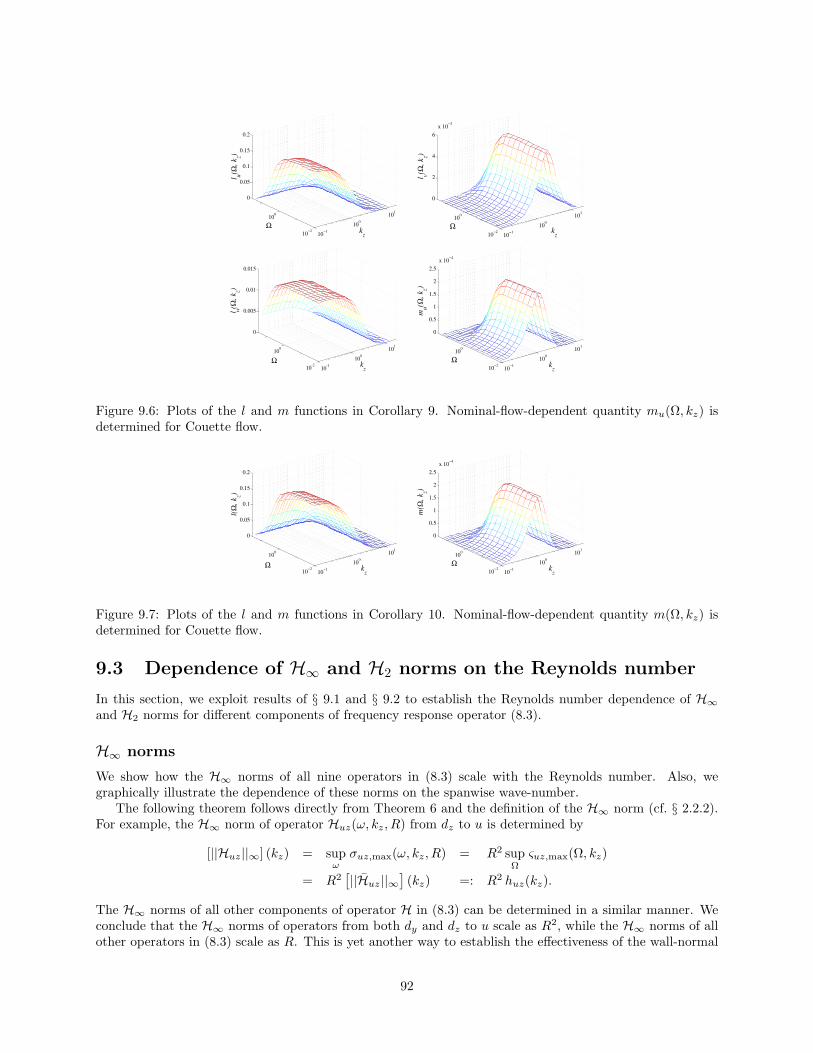
10−1
100
101
10−2
100
0
0.05
0.1
0.15
0.2
kz
Ωl u(Ω
, kz)
10−1
100
101
10−2
100
0
2
4
6x 10
−3
kz
Ω
l v(Ω, k
z)
10-1
100
101
10-2
100
0
0.005
0.01
0.015
kz
Ω
l w(Ω
, kz)
10−1
100
101
10−2
100
0
0.5
1
1.5
2
2.5
x 10−4
kz
Ω
mu(Ω
, kz)
Figure 9.6: Plots of the l and m functions in Corollary 9. Nominal-flow-dependent quantity mu(Ω, kz) isdetermined for Couette flow.
10−1
100
101
10−2
100
0
0.05
0.1
0.15
0.2
kz
Ω
l(Ω
, kz)
10−1
100
101
10−2
100
0
0.5
1
1.5
2
2.5
x 10−4
kz
Ω
m(Ω
, kz)
Figure 9.7: Plots of the l and m functions in Corollary 10. Nominal-flow-dependent quantity m(Ω, kz) isdetermined for Couette flow.
9.3 Dependence of H∞ and H2 norms on the Reynolds number
In this section, we exploit results of § 9.1 and § 9.2 to establish the Reynolds number dependence of H∞and H2 norms for different components of frequency response operator (8.3).
H∞ norms
We show how the H∞ norms of all nine operators in (8.3) scale with the Reynolds number. Also, wegraphically illustrate the dependence of these norms on the spanwise wave-number.
The following theorem follows directly from Theorem 6 and the definition of the H∞ norm (cf. § 2.2.2).For example, the H∞ norm of operator Huz(ω, kz, R) from dz to u is determined by
[||Huz||∞] (kz) = supωσuz,max(ω, kz, R) = R2 sup
Ωςuz,max(Ω, kz)
= R2[||Huz||∞
](kz) =: R2 huz(kz).
The H∞ norms of all other components of operator H in (8.3) can be determined in a similar manner. Weconclude that the H∞ norms of operators from both dy and dz to u scale as R2, while the H∞ norms of allother operators in (8.3) scale as R. This is yet another way to establish the effectiveness of the wall-normal
92

Table 9.1: Dependence of supkz[||Huy||∞] (kz) and supkz
[||Huz||∞] (kz) on R in Poiseuille and Couette flows.The values of kz at which global maxima take place are also shown.
Flow supkz[||Huy||∞] (kz) kz
Poiseuille (R/20.29)2 1.95Couette (R/10.29)2 1.55
Flow supkz[||Huz||∞] (kz) kz
Poiseuille (R/19.49)2 1.20Couette (R/8.81)2 1
and spanwise forces, and the largest energy content of the streamwise velocity perturbations.
Theorem 11 For any streamwise constant channel flow with nominal velocity U(y), the H∞ norms ofoperators Hrs(ω, kz, R) that map ds into r, r = u, v, w; s = x, y, z, are given by
[||Hux||∞] (kz) [||Huy||∞] (kz) [||Huz||∞] (kz)
[||Hvx||∞] (kz) [||Hvy||∞] (kz) [||Hvz||∞] (kz)
[||Hwx||∞] (kz) [||Hwy||∞] (kz) [||Hwz||∞] (kz)
=
hux(kz)R huy(kz)R2 huz(kz)R2
0 hvy(kz)R hvz(kz)R0 hwy(kz)R hwz(kz)R
,
where the h functions are independent of R.
We note that Kreiss, Lundbladh & Henningson showed in [10] that the H∞ norm of the resolvent(sI − A)−1 of the streamwise constant LNS system (9.1) can be upper bounded by a term that growsproportionally to R2 in the limit as R → ∞. On the other hand, by considering operators from theindividual forcing components to the individual velocity components, we explicitly established how the H∞norms of these operators at kx = 0 scale with the Reynolds number. This once again displays advantages ofcomponentwise analysis over the analysis that only accounts for the aggregate effects.
Figure 9.8 graphically illustrates the kz–dependence of functions hrs, r = u, v, w; s = x, y, z, inTheorem 11. Clearly, the nominal-velocity dependent quantities huy and huz play the most important rolesin high Reynolds number flows. Table 9.1 shows how supkz
[||Huy||∞] (kz) and supkz[||Huz||∞] (kz) scale
with R in both Poiseuille and Couette flows. The values of kz at which global maxima occur are also shown.
H2 norms
We study the frequency responses (as a function of kz) of each of the components of the transfer function(8.3). We do this using the H2 norm, that is
[‖Hrs‖2
2
](kz) :=
12π
∫ ∞
−∞||Hrs(kz, ω)||2HS dω, for r = u, v, w, and s = x, y, z.
We then investigate the dependence of each of the subsystems on the Reynolds number. We conclude thatamplification from both spanwise and wall-normal forcing to streamwise velocity is O(R3), while amplificationfor all other components is O(R).
We now state the main result that follows directly from Theorem 7 using the definition of the H2 norm.
Theorem 12 For any streamwise constant channel flow with nominal velocity U(y), the H2 norms of oper-
93
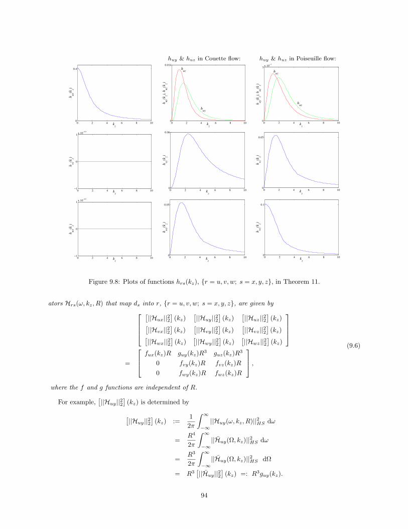
huy & huz in Couette flow: huy & huz in Poiseuille flow:
0 2 4 6 8 100
0.4
kz
h ux(k
z)
0 2 4 6 8 100
0.014
kz
h uy(k
z), h uz
(kz)
huz
huy
0 2 4 6 8 100
3x 10
−3
kz
h uy(k
z), h uz
(kz)
huz
huy
0 2 4 6 8 10−1
0
1x 10
−10
kz
h vx(k
z)
0 2 4 6 8 100
0.06
kz
h vy(k
z)
0 2 4 6 8 100
0.05
kz
h vz(k
z)0 2 4 6 8 10
−1
0
1x 10
−10
kz
h wx(k
z)
0 2 4 6 8 100
0.05
kz
h wy(k
z)
0 2 4 6 8 100
0.1
kz
h wz(k
z)
Figure 9.8: Plots of functions hrs(kz), r = u, v, w; s = x, y, z, in Theorem 11.
ators Hrs(ω, kz, R) that map ds into r, r = u, v, w; s = x, y, z, are given by
[||Hux||22
](kz)
[||Huy||22
](kz)
[||Huz||22
](kz)[
||Hvx||22](kz)
[||Hvy||22
](kz)
[||Hvz||22
](kz)[
||Hwx||22](kz)
[||Hwy||22
](kz)
[||Hwz||22
](kz)
=
fux(kz)R guy(kz)R3 guz(kz)R3
0 fvy(kz)R fvz(kz)R0 fwy(kz)R fwz(kz)R
,
(9.6)
where the f and g functions are independent of R.
For example,[||Huy||22
](kz) is determined by
[||Huy||22
](kz) :=
12π
∫ ∞
−∞||Huy(ω, kz, R)||2HS dω
=R4
2π
∫ ∞
−∞||Huy(Ω, kz)||2HS dω
=R3
2π
∫ ∞
−∞||Huy(Ω, kz)||2HS dΩ
= R3[||Huy||22
](kz) =: R3guy(kz).
94

0 2 4 6 8 100
0.05
0.1
0.15
0.2
0.25
0.3
0.35
kz
f ux(k
z)
0 2 4 6 8 100
0.2
0.4
0.6
0.8
1
1.2
1.4
1.6x 10
-4
kz
g uy(k
z)
0 2 4 6 8 100
0.5
1
1.5
2
2.5x 10
-4
kz
g uz(k
z)
0 2 4 6 8 101
0
1x 10
-10
kz
f vx(k
z)
0 2 4 6 8 100
0.005
0.01
0.015
0.02
0.025
0.03
kz
f vy(k
z)
0 2 4 6 8 100
0.005
0.01
0.015
0.02
kz
f vz(k
z)
0 2 4 6 8 101
0
1x 10
-10
kz
f wx(k
z)
0 2 4 6 8 100
0.005
0.01
0.015
0.02
kz
f wy(k
z)
0 2 4 6 8 100
0.02
0.04
0.06
0.08
0.1
0.12
0.14
kz
f wz(k
z)
Figure 9.9: Plots of frs(kz), r = u, v, w; s = x, y, z, guy(kz), and guz(kz). Functions guy(kz) and guz(kz)are determined for Couette flow.
Similar procedure can be used to determine the H2 norms of all other components of operator H in (8.3),which proves Theorem 12. Corollaries 13, 14, and 15 follow from Theorem 12 using the square-additivity ofthe H2 norm.
The energy amplification of streamwise constant perturbations scales as R3 from the forces in the wall-normal and the spanwise directions to the streamwise velocity. In all other cases it scales as R. In particular,at kx = 0 the streamwise direction forcing does not influence the wall-normal and the spanwise velocitycomponents. This further illustrates the dominance of the streamwise velocity perturbations and the forcesin the remaining two spatial directions for high Reynolds number channel flows.
The expressions for the terms that multiply R in (9.6) are the same for all channel flows. On the otherhand, the expressions for guy and guz depend on the coupling operator (vortex stretching term from the NSequations) Cp := −ikzU ′(y), and therefore these terms are nominal-velocity dependent. Whenever eitherthere is no mean shear or spanwise variations in the velocity perturbations, the vortex tilting mechanism isabsent and the largest amplification that can be achieved is proportional to the Reynolds number.
The following corollary of Theorem 12 is obtained by summing the rows in (9.6) and exploiting the squareadditive property of the H2 norm.
Corollary 13 For any streamwise constant channel flow with nominal velocity U(y), the H2 norms ofoperators Hs(ω, kz, R) that map ds into φ :=
[u v w
]T , s = x, y, z, are given by[‖Hx‖2
2
](kz) = fx(kz)R,[
‖Hy‖22
](kz) = fy(kz)R + gy(kz)R3,[
‖Hz‖22
](kz) = fz(kz)R + gz(kz)R3,
(9.7)
95

0 2 4 6 8 100
0.05
0.1
0.15
0.2
0.25
0.3
0.35
kz
f s(kz)
fz
fy
fx
0 2 4 6 8 100
0.5
1
1.5
2
2.5x 10
-4
kz
g s(k
z)
g z
g y
0 2 4 6 8 100
0.5
1
1.5
2
2.5
3
3.5x 10
-5
kz
g s(k
z)
g y
g z
Figure 9.10: The kz–dependence of fx, fy, fz, gy, and gz. Expressions for fx, fy, and fz are the same forall channel flows, as demonstrated in § 9.6.2. The terms responsible for the O(R3) energy amplification areshown in the middle (Couette flow) and right (Poiseuille flow) plots.
wherefx := fux, fy := fvy + fwy, fz := fvz + fwz,
gy := guy, gz := guz.
Figure 9.10 graphically illustrates the kz–dependence of functions fx, fy, fz, gy, and gz. Expressions forfx, fy, and fz are the same for all channel flows, as shown in § 9.6.2 where we derive the analytical formulae forthese quantities. On the other hand, both gy and gz depend on the nominal velocity. In § 9.6.2, we determinethe analytical expressions for these two quantities in Couette flow by doing the spectral decompositions ofthe Orr-Sommerfeld and Squire operators. These expressions are given in terms of rapidly convergent seriesand they are shown in the middle plot of Figure 9.10. The numerically computed dependence of gy and gzon kz in Poiseuille flow is given in the right plot of the same figure.
Therefore, as already indicated by the numerical computations of Chapter 8, the forces in the spanwiseand wall-normal directions have the strongest influence on the velocity field. We confirmed this observationby analytical derivations summarized in Corollary 13 for the streamwise constant perturbations showing thatthe square of the H2 norm from dz and dy to velocity vector φ scales as R3. On the other hand, at kx = 0,the square of the H2 norm from dx to φ scales as R.
The following corollary of Theorem 12 is obtained by summing the collumns in (9.6) and exploiting thesquare additive property of the H2 norm.
Corollary 14 For any streamwise constant channel flow with nominal velocity U(y), the H2 norms ofoperators Hr(ω, kz, R) that map d :=
[dx dy dz
]T into r, r = u, v, w, are given by[‖Hu‖2
2
](kz) = fu(kz)R + gu(kz)R3,[
‖Hv‖22
](kz) = fv(kz)R,[
‖Hw‖22
](kz) = fw(kz)R,
(9.8)
wherefu := fux, gu := guy + guz,
fv := fvy + fvz, fw := fwy + fwz.
Figure 9.11 graphically illustrates the kz–dependence of functions fu, fv, fw, and gu. Expressions for fu,fv, and fw are the same for all channel flows, as shown in § 9.6.2 where we derive the analytical formulaefor these quantities. On the other hand, gu depends on the underlying mean velocity. In § 9.6.2, we derivethe analytical dependence of gu on kz for Couette flow. The right plot in Figure 9.11 shows the numericallycomputed kz–dependence of gu in Poiseuille flow.
Thus, the impact of the external excitations is most powerful on the streamwise velocity component.We confirmed this observation by both numerical computations of Chapter 8 and analytical derivations
96

0 2 4 6 8 100
0.05
0.1
0.15
0.2
0.25
0.3
0.35
kz
f r (k z )
f v
fw
f u
0 2 4 6 8 100
0.5
1
1.5
2
2.5
3
3.5x 10
-4
kz
g u(kz)
0 2 4 6 8 100
1
2
3
4
5x 10
-5
kz
g u(k
z)
Figure 9.11: The kz–dependence of fu, fv, fw, and gu. Expressions for fu, fv, and fw are the same forall channel flows, as demonstrated in § 9.6.2. The terms responsible for the O(R3) energy amplification areshown in the middle (Couette flow) and right (Poiseuille flow) plots.
summarized in Corollary 14 for the streamwise constant perturbations showing that the square of the H2
norm from d to u scales as R3. On the other hand, at kx = 0, the square of the H2 norm from d to v andw scales as R.
It is worth mentioning that Theorem 1 of [11] follows from Theorem 12 of this section. Namely, bysumming all elements in (9.6) and using the square-additivity of the H2 norm the aggregate effect of allforces to all velocity components is readily obtained. For completeness, we state the main result of [11] asthe following corollary.
Corollary 15 For any streamwise constant channel flow with nominal velocity U(y), the H2 norm of oper-ator H(ω, kz, R) that maps d :=
[dx dy dz
]T into φ :=[u v w
]T , is given by[‖H‖2
2
](kz) = f(kz)R + g(kz)R3,
where
f := fux + fvy + fvz + fwy + fwz = fx + fy + fz = fu + fv + fw,
g := guy + guz = gy + gz = gu.
As shown in § 9.4, the dependence of the variance amplification on the Reynolds number at kx = 0 hasthe same form for the ‘unstructured’ and ‘structured’ external excitations. However, the expressions forfunctions f and g in Theorem 12 and Corollaries 13, 14, and 15 are different in these two cases.
In § 9.4, we study the capability of the streamwise constant near-wall input components.
9.4 Energy amplification of near-wall external excitations
In this section, we study system (7.20) in the presence of streamwise constant three-dimensional perturba-tions. By setting kx = 0 in (7.20) we obtain
∂t
[ψ1
ψ2
]=
[1RL 0
Cp 1RS
] [ψ1
ψ2
]+
[0 By01 Bz01
Bx02 0 0
] dx0dy0dz0
, (9.9a)
uvw
=
0 Cu2
Cv1 0Cw1 0
[ ψ1
ψ2
], (9.9b)
withBx02 := ikzκx(y), By01 := −k2
z∆−1κy(y), Bz01 := −ikz∆−1(κ′z(y) + κz(y)∂y),
97

where κs(y), for every s = x, y, z, denote arbitrary functions of y, and κ′z(y) := dκz(y)/dy. All otheroperators have the same meaning as in (9.1).
Since operators A, B, and C in (9.1) and (9.9) have the same respective structures, we conclude that alltheorems and corollaries of § 9.1, § 9.2, and § 9.3 that determine scaling with R for different measures ofinput-output amplification also hold for system (9.9). However, the expressions for the Reynolds numberindependent quantities are different for the ‘unstructured’ and ‘structured’ external excitations.
Effectiveness of near-wall external excitations
We next investigate the effectiveness of an input applied in a certain spatial direction by studying theReynolds number dependence of
[‖Hs‖2
2
](kz), where
Hs(ω, kz) := C(kz)(iωI − A(kz))−1Bs0(kz), s = x, y, z.
Based on the above remarks, it follows that Corollary 13 holds for both ‘unstructured’ and ‘structured’external excitations. However, the expressions for functions fx, fy, fz, gy, and gz are different in these twocases. This is illustrated in § 9.6.2 where we derive analytical expressions for fx, fy, fz (which are the samefor all channel flows) for
κs(y) := a(1 + coth(a))e−a(y+1) =: κ(y, a), a > 0, ∀ s = x, y, z, (9.10)
and determine the dependence of gy and gz on both kz and a in terms of easily computable series in Couetteflow. This particular ‘pre-modulation’ in y is chosen to analyze the effectiveness of inputs whose amplitudedecays exponentially away from the lower wall. Clearly, this rate of decay (i.e., degree of localization) canbe adjusted by assigning different values to parameter a. We note that functions f and g in Corollary 13now depend on both kz and ‘modulation parameter’ a, e.g. fx = fx(kz, a).
We have normalized κ(y, a) so that
∫ 1
−1
κ(y, a) dy = 2, ∀ a > 0,
which allows for comparison between ‘structured’ (in the limit as a→ 0) and ‘unstructured’ results. Clearly,in the ‘unstructured’ case there is no ‘pre-modulation’ in y, that is
κ(y) ≡ 1 ⇒∫ 1
−1
κ(y) dy = 2.
The formulae for functions fx(kz, a), fy(kz, a), and fz(kz, a) are determined in § 9.6.2. Furthermore,the traces of nominal-velocity-dependent operators are determined in terms of rapidly convergent series forCouette flow in § 9.6.2.
The analytical expression for fx(kz, a) is given by (9.35). By taking the limit of fx(kz, a) as a → 0 weobtain (9.29) which corresponds to the value of fx(kz) for ‘unstructured’ external excitation. Furthermore,as kz → ∞, we have
limkz→∞
fx(kz, a) = 0, ∀ a ∈ (0, ∞),
which implies that for any finite value of a > 0 function fx(kz, a) decays to zero for big enough values of kz.On the other hand, a limit of fx(kz, a) as a→ ∞ is determined by
lima→∞ fx(kz, a) =
12, ∀ kz ∈ R,
which suggests that for external excitation that is localized in the vicinity of the lower wall (large enoughvalues of a) and acts in the streamwise direction influence of high spanwise wave numbers becomes more andmore important. This is illustrated in Figure 9.12 where we graphically illustrate the dependence of fx onkz for different values of a.
98

0 5 10 15 20 25 300
0.1
0.2
0.3
0.4
0.5
0.6
kz
f x
a → ∞
a → 0
a = 5
a = 10
a = 20
a = 100
0 5 10 15 20 25 300
0.1
0.2
0.3
0.4
0.5
0.6
kz
f z
a = 10
a → ∞
a = 100
a → 0 a = 5
a = 20
0 20 40 60 80 1000
0.005
0.01
0.015
0.02
0.025
0.03
0.035
0.04
0.045
kz
f y
a → 0
a = 5
a = 10
a = 20
0 200 400 600 800 10000
0.005
0.01
0.015
0.02
0.025
0.03
0.035
0.04
0.045
kz
f y a = 100
a = 200
Figure 9.12: The kz–dependence of fx, fy, and fz for different values of a.
log10(gy(kz, a)): log10(gz(kz, a)):
Figure 9.13: Plots of gy(kz, a), and gz(kz, a) in Couette flow.
The formulae for fy(kz, a) and fz(kz, a) are given by (9.36). The kz–dependence of these two quantitiesfor different values of a is shown in Figure 9.12. We note that the limits of fy(kz, a) and fz(kz, a) as a→ 0are in agreement with the corresponding formulae (9.30) for the ‘unstructured’ excitation.
The analytical expressions for gy(kz, a) and gz(kz, a) in Couette flow are determined in § 9.6.2. Theseformulae are expressed in terms of rapidly convergent series, and they are obtained by performing the spectraldecompositions of the Orr-Sommerfeld and Squire operators. Since R3 respectively multiplies gy(kz, a) andgz(kz, a) in the expressions for
[‖Hy‖2
2
](kz) and
[‖Hz‖2
2
](kz) (see Corollary 13), it is relevant to analyze
how gy(kz, a) and gz(kz, a) change with their arguments. Figure 9.13 shows the dependence of these twoquantities on both kz and a. Clearly, the magnitude of gy decreases sharply as a increases its value. On theother hand, the value of gz increases for a certain range of a’s and then it starts decaying at a very slow rate.Furthermore, for any fixed value of parameter a both gy and gz achieve largest values at O(1) values of kz.
In Figure 9.14, we illustrate the a–dependence of the following quantities
supkz
gy(kz, a), supkz
gz(kz, a),supkz
gz(kz, a)supkz
gy(kz, a),
99

0 20 40 60 80 10010
-8
10-7
10-6
10-5
10-4
10-3
a
sup k z
g y(k
z,a)
0 20 40 60 80 100
10-4
10-3
a
sup k z
g z(k
z,a)
0 20 40 60 80 10010
0
101
102
103
104
a
sup k z
g z(k
z,a)
/sup
k z g y
(kz,a
)
Figure 9.14: Plots of supkzgy(kz, a), supkz
gz(kz, a), and supkzgz(kz, a)/ supkz
gy(kz, a) in Couette flow.
in Couette flow, with the abscissa in the linear and the ordinate in the logarithmic scale. Clearly, supkzgy(kz, a)
decays monotonically as a function of a with a fairly sharp rate of decay, while supkzgz(kz, a) peaks at a
non-zero value of a and then decays slowly as a increases its value. The right plot further shows thatsupkz
gz(kz, a)/ supkzgy(kz, a) is a monotonically increasing function of a and that, for example, at a = 100
function supkzgz(kz, a) achieves almost four orders of magnitude larger value than function supkz
gy(kz, a).This indicates that the localized spanwise excitations have much stronger influence on the velocity field thanthe localized wall-normal excitations. This observation is consistent with recent numerical work on channelflow turbulence control using the Lorentz force [4–6], where it was concluded that forcing in the spanwisedirection confined within the viscous sub-layer had the strongest effect in suppressing turbulence. We con-firmed this observation by analytical derivations for the streamwise constant perturbations showing that thespanwise forcing localized near the lower wall has, by far, the strongest effect on the evolution of the velocityfield components.
9.5 Exact determination of Hilbert–Schmidt norms
In this section, we employ the analytical procedure developed in Chapter 3 to ascertain the Hilbert–Schmidtnorms of the Reynolds number independent operators Hrs(Ω, kz), r = u, v, w; s = x, y, z. We note thatHux(Ω, kz) has a second order state-space realization, the operators Hrs(Ω, kz), r = v, w; s = y, z, canbe represented by the fourth order TPBVSR, while Huy(Ω, kz) and Huz(Ω, kz) can be described by minimalrealizations with six states. These realizations can be chosen in a number of different ways. Realizationsthat we use are given in § 9.5.1. It is noteworthy that the Hilbert-Schmidt norms of these operators forany given pair (Ω, kz) can be determined explicitly using the procedure of § 3.2.3 which involves only finitedimensional computations with matrices whose dimension is at most four times larger than the order ofthe underlying operators. Therefore, in the worst case we need to determine the state transition matricesthat belong to C
24×24, which can be easily done, for example in matlab. This illustrates the power of theprocedure developed in Chapter 3 and circumvents the need for numerical approximation of the underlyingoperators.
In Couette flow, the coupling operator simplifies to Cp = −ikz and, thus, all operators in (9.1) have theconstant coefficients in y. As a result, matrix A0 in (9.13) no longer depends on the wall-normal coordinate.Hence, the nominal-flow-dependent quantitiesmuy andmuz can be determined explicitly using formula (3.19)which only requires determination of certain matrix exponentials. In other words, in streamwise constantCouette flow, each operator HrsH∗
rs can be represented by a well-posed TPBVSR with constant coefficientsin y
HrsH∗rs :
q′(y) = Aq(y) + Bsfs(y),
φr(y) = Crq(y),
0 = L1q(−1) + L2q(1), y ∈ [−1, 1],
100

which implies that ||Hrs(Ω, kz)||2HS is determined by (cf. (3.19) in Theorem 2)
||Hrs(Ω, kz)||2HS = − tr(
(L1 + L2e2A)−1L2
[0 I
]exp
2[
A 0BsCr A
][I
0
]).
9.5.1 State-space realizations of the linearized Navier-Stokes equations
Here, we describe the TPBVSR that are used for the frequency response determination of the streamwiseconstant LNS equations. Once the temporal Fourier transform has been applied, (9.1a) can be rewritten as
ψ1 = R(iΩI − L)−1(Bydy + Bzdz), (9.11a)
ψ2 = R(iΩI − S)−1(Cpψ1 + Bxdx), (9.11b)
with Ω := ωR. Since the Reynolds number enters conveniently into the equations, we can study (9.11) atR = 1, and rewrite it as
ψ(4)1 − (2k2
z + iΩ)ψ′′1 + k2
z(k2z + iΩ)ψ1 =
[k2z 0
] [ dydz
]+[
0 ikz] [ d′y
d′z
], (9.12a)
ψ′′2 − (k2
z + iΩ)ψ2 = ikzU ′(y)ψ1 − ikzdx. (9.12b)
Equations (9.12a) and (9.12b) are ODEs in y parameterized by kz and Ω with the boundary conditions
ψ1(±1) = ψ′1(±1) = ψ2(±1) = 0.
For notational convenience, we have suppressed the dependence of ψi and ds on kz and Ω, e.g. ψi(y) :=ψi(y,Ω, kz), i = 1, 2. Similarly, ψ(r)
i (y) := drψi(y,Ω, kz)/dyr.In particular, we choose the following realizations of (9.12a) and (9.12b)
(9.12a) :
ξ′(y) = A1ξ(y) + B1
dx(y)dy(y)dz(y)
,
ψ1(y) = C1ξ(y),
0 = S1ξ(−1) + S2ξ(1), y ∈ [−1, 1],
(9.12b) :
η′(y) = A2η(y) + B2
dx(y)dy(y)dz(y)
+ B3(y)ψ1(y),
ψ2(y) = C2η(y),
0 = T1η(−1) + T2η(1), y ∈ [−1, 1],
where
A1 :=
0 1 0 02k2z + iΩ 0 1 00 0 0 1
−k2z(k
2z + iΩ) 0 0 0
, A2 :=
[0 1
k2z + iΩ 0
],
B1 :=
0 0 00 0 00 0 ikz0 k2
z 0
, B2 :=
[0 0 0
−ikz 0 0
], B3(y) :=
[0
ikzU ′(y)
],
C1 :=[
1 0 0 0], C2 :=
[1 0
],
101

S1 :=
[I2×2 02×2
02×2 02×2
], S2 :=
[02×2 02×2
I2×2 02×2
], T1 :=
[1 00 0
], T2 :=
[0 01 0
].
We now combine these two realization with (9.1b) to obtain a TPBVSR of operator H at (kx = 0, R = 1)
(9.12, 9.1b) :
x′(y) = A0(y)x(y) + B0
dx(y)dy(y)dz(y)
,
u(y)v(y)w(y)
= C0x(y),
0 = N1x(−1) + N2x(1), y ∈ [−1, 1],
(9.13)
where xT (y) :=[ξT (y) ηT (y)
], and
A0(y) :=[
A1 0B3(y)C1 A2
]=
0 1 0 0 0 02k2z + iΩ 0 1 0 0 00 0 0 1 0 0
−k2z(k
2z + iΩ) 0 0 0 0 00 0 0 0 0 1
ikzU ′(y) 0 0 0 k2z + iΩ 0
,
B0 :=[B1
B2
]=
0 0 00 0 00 0 ikz0 k2
z 00 0 0
−ikz 0 0
=:[Bx0 By0 Bz0
], N1 :=
[S1 00 T1
],
C0 :=
0 0 0 0 − ikz
01 0 0 0 0 00 i
kz0 0 0 0
=:
Cu0
Cv0
Cw0
, N2 :=
[S2 00 T2
].
Thus, we have rendered TPBVSR of system (9.12,9.1b) into (9.13), which is a suitable form for the applicationof the procedure developed in Chapter 3.
The realizations of Hrs(Ω, kz) can be now easily determined for every r = u, v, w; s = x, y, z. Forexample, TPBVSR of Huy(Ω, kz) is given by
Huy :
x′(y) = A0(y)x(y) + By0dy(y),
u(y) = Cu0x(y),
0 = N1x(−1) + N2x(1), y ∈ [−1, 1].
As previously mentioned, Hux(Ω, kz) and Hrs(Ω, kz), for every r = v, w; s = y, z, are respectively thesecond and the fourth order operators. We note that their minimal realizations can be obtained by combiningthe respective realizations of (9.12b) and (9.12a) with the corresponding rows of (9.1b). For example, a
102

minimal realization of Hux(Ω, kz) is given by
Hux :
η′(y) =
[0 1
k2z + iΩ 0
]η(y) +
[0
−ikz
]dx(y),
u(y) =[− ikz
0]η(y),
0 = T1η(−1) + T2η(1), y ∈ [−1, 1].
Alternatively, ||Hux(Ω, kz)||2HS can be determined from Theorem 2 using the following non-minimal realiza-tion of Hux(Ω, kz)
Hux :
x′(y) = A0(y)x(y) + Bx0dx(y),
u(y) = Cu0x(y),
0 = N1x(−1) + N2x(1), y ∈ [−1, 1].
Figure 9.3 in § 9.2 illustrates the plots of ||Hrs(Ω, kz)||2HS , for every r = u, v, w; s = x, y, z. Thesecomputations are performed in matlab for any given pair (Ω, kz) using the procedure developed in Chapter 3with the above TPBVSR.
In § 9.5.2, we derive analytical expressions for functions ||Hrs(0, kz)||2HS .
9.5.2 Formulae for Hilbert–Schmidt norms at ω = 0
In this subsection, we derive explicit expressions for the Hilbert-Schmidt norms of streamwise constantsteady-state perturbations. As shown in § 9.2, these perturbations experience the largest amplificationrates. Formulae for functions lrs(0, kz) and mrs(0, kz) in (9.4) are determined symbolically in mathematicausing (3.19). The mean-flow-dependent quantitiesmuy andmuz are obtained for Couette flow. The analyticalexpressions are given by
lux(0, kz) =kz(coth(2kz) + 2kzcsch2(2kz)
)− 1
2k4z
,
muy(0, kz) =cuy(kz)
322560k8z(cosh(4kz) − 8k2
z − 1)2,
muz(0, kz) =cuz(kz)
5160960k8z(cosh(4kz) − 8k2
z − 1)2,
lvy(0, kz) =cvy(kz)
1440k4z(cosh(4kz) − 8k2
z − 1)2,
lvz(0, kz) =cvz(kz)
1440k4z(cosh(4kz) − 8k2
z − 1)2,
lwy(0, kz) = lvz(0, kz),
lwz(0, kz) =cwz(kz)
1440k4z(cosh(4kz) − 8k2
z − 1)2,
103

where
cuy(kz) := − 297675 + 16k2z
(−187425 + 4k2
z
(−168525 + 8k2
z
(−8337 + 2474k2
z + 80k4z
)))+ 12
(33075 + 249900k2
z + 42000k4z + 28672k6
z + 768k8z
)cosh(4kz) − 99225 cosh(8kz)
+78kzcsch2(kz)sech2(kz)(3072k5
z(45 + 16k4z)
+ (14175 + 64k2z(2295 + 660k2
z − 1176k4z + 1216k6
z)) sinh(4kz)+ 12(−945 + 8k2
z(−765 + 440k2z + 72k4
z)) sinh(8kz) + 2835 sinh(12kz)),
cuz(kz) := + csch2(kz)sech2(kz)(34650 + 16k2z(31185 + 4k2
z(2835 + 16k2z(630 + 2577k2
z − 592k4z)))
− (51975 + 64k2z(10395 + 8k2
z(735 − 70k2z + 1776k4
z + 160k6z))) cosh(4kz)
+ 20790 cosh(8kz) − 3465 cosh(12kz) + 2kz(8kz(10395 + 12180k2z − 2240k4
z − 576k6z) cosh(8kz)
+ 224(315 cosh(2kz)sinh(2kz)5 + k2
z(2(855 + 8k2z(45 + 197k2
z − 136k4z)) sinh(4kz)
+ (−855 + 180k2z − 136k4
z) sinh(8kz))))),cvy(kz) := − 1485 + 8k2
z
(−1845 + 128k2
z
(−45 + 2k2
z
(−8 + k2
z
)))− 495 cosh(8kz)
+ 4(495 + 3690k2
z + 720k4z + 256k6
z
)cosh(4kz)
+ 30kz(−15 − 216k2
z + 128k4z + 15 cosh(4kz)
)sinh(4kz),
cvz(kz) := − 135 − 8k2z
(225 − 128k4
z + 256k6z
)+ 4
(45 + 450k2
z + 720k4z − 256k6
z
)cosh(4kz)
− 45 cosh(8kz) + 90kz(−1 − 40k2
z + cosh(4kz))sinh(4kz),
cwz(kz) := − 135 + 8k2z
(−225 + 16k2
z
(−5 + 4k2
z
) (3 + 4k2
z
))− 45 cosh(8kz)
+ 4(45 + 450k2
z + 1200k4z + 256k6
z
)cosh(4kz)
− 30kz(3 + 120k2
z + 128k4z − 3 cosh(4kz)
)sinh(4kz).
Formulae for functions lx, ly, lz,my,mz, lu, lv, lw,mu, and l,m can be readily obtained by combiningtheir respective definitions from Corollaries 8, 9, and 10 with the above expressions.
9.6 Exact determination of H2 norms
In § 9.6.1, we derive expressions for the componentwise H2 norms of streamwise constant LNS system (9.1)in terms of solutions to the corresponding Lyapunov equations. In § 9.6.2, we utilize these relationships todetermine the explicit kz–dependence of functions f and g in Corollaries 13 and 14 for both ‘unstructured’and ‘structured’ external excitations. The nominal-flow-dependent functions g are determined in Couetteflow. The main analytical tool we use in § 9.6.2 is the formula for the trace of a class of differential operatorsdefined by forced TPBVSR. This formula is derived in § 3.2.2.
From § 7.1.2 and § 9.1, it follows that at kx = 0
A =
[1R∆−1∆2 0
−ikzU ′ 1R∆
]=:
[1RL 0
Cp 1RS
],
A∗ =
[1R∆−1∆2 −ikz∆−1U ′
0 1R∆
]=:
[1RL C∗
p
0 1RS
],
Mx = Nu =
[0 0
0 I
], My = Nv =
[−k2
z∆−1 0
0 0
], Mz = Nw =
[∆−1∂yy 0
0 0
],
where operators Ms and Nr are defined as Ms := BsB∗s , for s = x, y, z, and Nr := C∗
rCr, for r = u, v, w.
104

The results of this section also hold for system (7.20) with ‘structured’ external excitations since operators
Bx0B∗x0 =
[0 0
0 κ2u
], By0B∗
y0 =
[−k2
z∆−1κ2
v 0
0 0
],
Bz0B∗z0 =
[∆−1(2κwκ′w∂y + κ2
w∂yy) 0
0 0
],
have the same respective structures as operators Mx, My, and Mz. As remarked in § 9.4, the dependenceof the variance amplification on the Reynolds number at kx = 0 has the same form for the ‘unstructured’ and‘structured’ external excitations. However, the expressions for functions f and g in Theorem 12, Corollary 13,and Corollary 14 are different in these two cases.
9.6.1 Expressions for H2 norms via Lyapunov equations
In this subsection, we provide alternative proofs of Theorem 12, Corollary 13, and Corollary 14 by exploitingthe fact that the H2 norms of frequency response operators Hrs, Hs, and Hr, r = u, v, w; s = x, y, z, canbe determined based on solutions of the corresponding Lyapunov equations. The procedure outlined belowis most convenient for determination of the Reynolds number independent functions f and g in (9.6), (9.7),and (9.8).
Controllability Gramians and functions f and g in Theorem 12
For each r and s,[‖Hrs‖2
2
](kz) can be expressed in terms of the solution to an operator Lyapunov equation
of the formAXs + XsA∗ = −Ms (9.14)
as[‖Hrs‖2
2
](kz) = trace(NrXs), where Xs is a 2 × 2 block operator whose structure we denote by
Xs :=
[Xs11 X ∗
s0
Xs0 Xs22
].
Using the structure of operators Nr and Xs it follows that[‖Hrs‖2
2
](kz) can be determined as[
‖Hrs‖22
](kz) = trace(NrXs) = trace(Nr11Xs11) + trace(Nr22Xs22).
The lower block triangular structure of A transforms (9.14) into the set of conveniently coupled operatorSylvester equations of the form
LXs11 + Xs11L = −RMs11, (9.15a)SXs0 + Xs0L = −RCpXs11, (9.15b)
SXs22 + Xs22S = −R(Ms22 + CpX ∗s0 + Xs0C∗
p). (9.15c)
If the solutions of this system of equations at R = 1 are respectively denoted by Ps11, Ps0, and Ps22, then(9.15) simplifies to
LPs11 + Ps11L = −Ms11, (9.16a)SPs0 + Ps0L = − CpPs11, (9.16b)
SPs222 + Ps222S = − (CpP∗s0 + Ps0C∗
p), (9.16c)
SPs221 + Ps221S = −Ms22, (9.16d)
where Ps22 = Ps221 + Ps222 . Clearly, equations (9.16a) and (9.16d) can be respectively solved for Ps11 andPs221 . Once Ps11 is determined, (9.16b) can be solved to yield Ps0. Finally, Ps0 can be used to determine
105

solution to (9.16c).Linearity of (9.15) implies that its solutions can be expressed in terms of solutions to (9.16) as
Xs11 = RPs11, Xs0 = R2Ps0, Xs22 = RPs221 + R3Ps222,
which yields[‖Hrs‖2
2
](kz) = (trace(Nr11Ps11) + trace(Nr22Ps221))R + trace(Nr22Ps222)R
3. (9.17)
Using the definitions of operators Nr and Ms, it follows that
Nu11 ≡ 0, Nv22 ≡ 0, Nw22 ≡ 0 ,
Px11 ≡ 0, Px222 ≡ 0Py221 ≡ 0, Pz221 ≡ 0
,
which in combination with (9.17) gives the following expressions for functions f and g in (9.6)fux(kz) guy(kz) guz(kz)
0 fvy(kz) fvz(kz)0 fwy(kz) fwz(kz)
=
trace(Nu22(kz)Px221(kz)) trace(Nu22(kz)Py222(kz)) trace(Nu22(kz)Pz222(kz))0 trace(Nv11(kz)Py11(kz)) trace(Nv11(kz)Pz11(kz))0 trace(Nw11(kz)Py11(kz)) trace(Nw11(kz)Pz11(kz))
.
(9.18)
These expressions are most convenient for determination of functions f and g in Corollary 13.
Observability Gramians and functions f and g in Theorem 12
Alternatively,[‖Hrs‖2
2
](kz) can be, for every r = u, v, w; s = x, y, z, expressed in terms of the solution to
an operator Lyapunov equation of the form
A∗Yr + YrA = −Nr (9.19)
as[‖Hrs‖2
2
](kz) = trace(YrMs), where Yr is a 2 × 2 block operator whose structure we denote by
Yr :=
[Yr11 Y∗
r0
Yr0 Yr22
].
Using the structure of operators Ms and Yr it follows that[‖Hrs‖2
2
](kz) can be determined as[
‖Hrs‖22
](kz) = trace(YrMs) = trace(Yr11Ms11) + trace(Yr22Ms22).
The lower block triangular structure of A renders (9.19) into the set of conveniently coupled operatorSylvester equations of the form
SYr22 + Yr22S = −RNr22, (9.20a)SYr0 + Yr0L = −RYr22Cp, (9.20b)
LYr11 + Yr11L = −R(Nr11 + C∗pYr0 + Y∗
r0Cp). (9.20c)
106

If the solutions of this system of equations at R = 1 are respectively denoted by Rr22, Rr0, and Rr11, then(9.20) simplifies to
SRr22 + Rr22S = −Nr22, (9.21a)SRr0 + Rr0L = −Rr22Cp, (9.21b)
LRr112 + Rr112L = − (C∗pRr0 + R∗
r0Cp), (9.21c)
LRr111 + Rr111L = −Nr11, (9.21d)
where Rr11 = Rr111 +Rr112 . Clearly, equations (9.21a) and (9.21d) can be respectively solved for Rr22 andRr111 . Once Rr22 is determined, (9.21b) can be solved to yield Rr0. Finally, Rr0 can be used to determinethe solution to (9.21c).
Linearity of (9.20) implies that its solutions can be expressed in terms of solutions to (9.21) as
Yr22 = RRr22, Yr0 = R2Rr0, Yr11 = RRr111 + R3Rr112,
which yields[‖Hrs‖2
2
](kz) = (trace(Rr22Ms22) + trace(Rr111Ms11))R + trace(Rr112Ms11)R3. (9.22)
Using the definitions of operators Ms, and Nr, it follows that
Mx11 ≡ 0, My22 ≡ 0, Mz22 ≡ 0 ,Ru111 ≡ 0, Rv22 ≡ 0, Rv112 ≡ 0 , Rw22 ≡ 0, Rw112 ≡ 0 ,
which in combination with (9.22) gives the following expressions for functions f and g in (9.6)fux(kz) guy(kz) guz(kz)
0 fvy(kz) fvz(kz)0 fwy(kz) fwz(kz)
=
trace(Ru22(kz)Mx22(kz)) trace(Ru112(kz)My11(kz)) trace(Ru112(kz)Mz11(kz))0 trace(Rv111(kz)My11(kz)) trace(Rv111(kz)Mz11(kz))0 trace(Rw111(kz)My11(kz)) trace(Rw111(kz)Mz11(kz))
.
(9.23)
These expressions are most convenient for determination of functions f and g in Corollary 14.
Expressions for functions f and g in Corollary 13 via Lyapunov equations
Corollary 13 follows from Theorem 12 and square additivity of the H2 norm. Thus, for every s = x, y, z, theH2 norm of operator Hs from ds to φ :=
[u v w
]T is given by[||Hs||22
](kz) =
[||Hus||22
](kz) +
[||Hvs||22
](kz) +
[||Hws||22
](kz). (9.24)
Therefore, combination of (9.18) and (9.24) with
Nu22 = Nv11 + Nw11 = I,
yields [‖Hx‖2
2
](kz) = trace(Px221(kz))R =: fx(kz)R,[
‖Hy‖22
](kz) = trace(Py11(kz))R + trace(Py222(kz))R
3 =: fy(kz)R + gy(kz)R3,[‖Hz‖2
2
](kz) = trace(Pz11(kz))R + trace(Pz222(kz))R
3 =: fz(kz)R + gz(kz)R3,
107

which provides an alternative proof of Corollary 13, and gives convenient expressions for functions fx, fy, fz,gy, gz in terms of solutions to the corresponding Lyapunov equations. In § 9.6.2, we combine these expressionswith the trace formula of § 3.2.2 to derive respective formulae for fx(kz), fy(kz), fz(kz), gy(kz), gz(kz) forLNS systems (9.1) and (9.9) with ‘unstructured’ and ‘structured’ external excitations. Functions gy and gzare determined in Couette flow.
Expressions for functions f and g in Corollary 14 via Lyapunov equations
Corollary 14 follows from Theorem 12 and square additivity of the H2 norm. Thus, for every r = u, v, w,the H2 norm of operator Hr from d :=
[dx dy dz
]T to r is given by[||Hr||22
](kz) =
[||Hrx||22
](kz) +
[||Hry||22
](kz) +
[||Hrz||22
](kz). (9.25)
Therefore, combination of (9.23) and (9.25) with
Mx22 = My11 + Mz11 = I,
yields[‖Hu‖2
2
](kz) = trace(Ru22(kz))R + trace(Ru112(kz))R
3 =: fu(kz)R + gu(kz)R3,[‖Hv‖2
2
](kz) = trace(Rv111(kz))R =: fv(kz)R,[
‖Hw‖22
](kz) = trace(Rw111(kz))R =: fw(kz)R,
which provides an alternative proof of Corollary 14, and gives convenient expressions for functions fu, fv,fw, and gu in terms of solutions to the corresponding Lyapunov equations. In § 9.6.2, we combine theseexpressions with the trace formula of § 3.2.2 to derive formulae for fu(kz), fv(kz), fw(kz), gu(kz) for LNSsystem (9.1) with ‘unstructured’ external excitations. Function gu is determined in Couette flow.
9.6.2 Formulae for operator traces
In this subsection, we derive analytical formulae for traces of operators that appear in the expressions for[‖Hs‖2
2
](kz), s = x, y, z, and
[‖Hr‖2
2
](kz), r = u, v, w. The main analytical tool we use here is the
formula for the trace of a class of differential operators defined by forced TPBVSR. This formula is given in§ 3.2.2. In the process, we exploit the fact that some of the traces of interest have already been determinedin [11].
Unstructured external excitations: determination of nominal velocity indepen-dent traces
For system (9.1) with ‘unstructured’ external excitations, the nominal velocity independent operators (whosetraces we want to determine) can be represented by a well-posed TPBVSR with constant coefficients in y
F :
x′(y) = Ax(y) + Bf(y),
g(y) = Cx(y),
0 = L1x(−1) + L2x(1), y ∈ [−1, 1].
(9.26)
Thus, the traces of these operators can be obtained using the trace formula (3.16) of § 3.2.2 as
trace(F) = tr(CB − (L1 + L2e2A)−1L2
[0 I
]exp
2[
A 0BC A
][I
0
]). (9.27)
This formula is employed to determine explicit analytical expressions for functions fr(kz), r = u, v, w, andfs(kz), s = x, y, z in Corollaries 13 and 14.
108

Formulae for fx(kz), fy(kz), and fz(kz)
We recall that fx(kz), fy(kz), and fz(kz) are determined by trace(Px221(kz)), trace(Py11(kz)), and trace(Pz11(kz)),where operators Px221 , Py11, and Pz11 respectively satisfy
SPx221 + Px221S = − I, (9.28a)
LPy11 + Py11L = − (−k2z∆
−1), (9.28b)
LPz11 + Pz11L = − ∆−1∂yy. (9.28c)
The solution of (9.28a) is given by Px221 = − 12S−1 which in turn implies [11]1
fx(kz) := trace(Px221(kz)) =2kz coth(2kz) − 1
4k2z
. (9.29)
On the other hand, application of Lemma 2 of [11] to equations (9.28b) and (9.28c) respectively yields
trace(Py11(kz)) = − 12trace(L−1(−k2
z∆−1)) =
k2z
2trace((∆2)−1),
trace(Pz11(kz)) = −12trace(L−1∆−1∂yy) = − 1
2trace((∆2)−1∂yy).
Therefore, the remaining problem amounts to determination of traces of operators (∆2)−1 and (∆2)−1∂yywhose definitions are given by
(∆2)−1 : f1 −→ g1 ⇔ f1 = g(4)1 − 2k2
zg′′1 + k4
zg1, g1(±1) = g′1(±1) = 0,
(∆2)−1∂yy : f2 −→ g2 ⇔ f ′′2 = g(4)2 − 2k2
zg′′2 + k4
zg2, g2(±1) = g′2(±1) = 0.
For notational convenience, we have suppressed the dependence of fi and gj on kz, e.g. fi(y) := fi(y, kz),i = 1, 2. Similarly, f (r)
i (y) := drfi(y, kz)/dyr.These two operators can be represented by their state-space realizations as follows
(∆2)−1 :
x′(y) =
0 0 0 −k4z
1 0 0 00 1 0 2k2
z
0 0 1 0
x(y) +
1000
f1(y),
g1(y) =[
0 0 0 1]x(y),
0 =[
02×2 I2×2
02×2 02×2
]x(−1) +
[02×2 02×2
02×2 I2×2
]x(1), y ∈ [−1, 1],
(∆2)−1∂yy :
z′(y) =
0 0 0 −k4z
1 0 0 00 1 0 2k2
z
0 0 1 0
z(y) +
0010
f2(y),
g2(y) =[
0 0 0 1]z(y),
0 =[
02×2 I2×2
02×2 02×2
]z(−1) +
[02×2 02×2
02×2 I2×2
]z(1), y ∈ [−1, 1].
The realizations of both operators are in form (9.26) and thus, formula (9.27) can be used to determinetheir traces. Since both realizations are parameterized by spanwise wave-number, the traces of underlyingoperators are kz–dependent as well. With the help of mathematica we obtain the following formulae for
1Expression (27) in [11] should read2kz coth(2kz) − 1
4k2z
.
109

trace(Py11(kz)) and trace(Pz11(kz)):
fy(kz) =k2z
2trace((∆2)−1) = −16k4
z + 24k2z + 3kz sinh(4kz) − 9 sinh2(2kz)
24k2z(4k2
z − sinh2(2kz)),
fz(kz) = −12trace((∆2)−1∂yy) =
16k4z − 3kz sinh(4kz) + 3 sinh2(2kz)
24k2z(4k2
z − sinh2(2kz)).
(9.30)
It worth mentioning that the above determined traces do not depend on the form of channel flow. Onthe other hand, the traces of operators Py222(kz) and Pz222(kz) (that is, gy(kz) and gz(kz)) are not nominalvelocity independent. Rather, they depend on the underlying channel flow through its dependence on U ′.The derivation of the analytical expressions for these traces in Couette flow is also given in this section.
Formulae for fu(kz), fv(kz), fw(kz), and gu(kz)
We recall that fu(kz), fv(kz), and fw(kz) are determined by trace(Ru22(kz)), trace(Rv111(kz)), and trace(Rw111(kz)),where operators Ru22, Rv111 , and Rw111 respectively satisfy
SRu22 + Ru22S = − I, (9.31a)
LRv111 + Rv111L = − (−k2z∆
−1), (9.31b)
LRw111 + Rw111L = − ∆−1∂yy. (9.31c)
Comparison of equations (9.28) and (9.31) implies
fu(kz) := trace(Ru22(kz)) = trace(Px221(kz)) =: fx(kz),fv(kz) := trace(Rv111(kz)) = trace(Py11(kz)) =: fy(kz),fw(kz) := trace(Rw111(kz)) = trace(Pz11(kz)) =: fz(kz),
where the expressions for fx, fy, and fz are given by (9.29) and (9.30). On the other hand, gu(kz) :=trace(Ru112(kz)) is a function of a nominal velocity. In Couette flow, the formula for gu(kz) can be obtainedby comparing the expression for
[‖H‖2
2
](kz) of § 9.3 with its counterpart of [11]. By doing so, we obtain the
following formula:
gu(kz) := trace(Ru112(kz)) =
14
∞∑n=1
k2z
γ4n
1 − n2π2
γn
[2kz(cosh(2kz) − 1)γn(sinh(2kz) − 2kz)
+1
4(αn coth(αn) − kz coth(kz))
]n even,
1 − n2π2
γn
[2kz(cosh(2kz) + 1)γn(sinh(2kz) + 2kz)
+1
4(αn tanh(αn) − kz tanh(kz))
]n odd,
where
γn := −(n2π2
4+ k2
z
), αn :=
√2k2z +
n2π2
4, n ≥ 1.
Our current efforts are directed towards development of the formula for gu(kz) in Poiseuille flow.
Structured external excitations: determination of nominal velocity independenttraces
In this subsection, we consider streamwise constant LNS system (9.9) with ‘structured’ external excitations,and derive the explicit analytical expressions for functions fx, fy, and fz in Corollary 13. This is done for ‘pre-modulation’ in the wall-normal direction defined by (9.10). In this case, the nominal velocity independent
110

operators (whose traces we want to determine) can be represented by a well-posed TPBVSR
F :
x′(y) = Ax(y) + e−2a(y+1)Bf(y),
g(y) = Cx(y),
0 = L1x(−1) + L2x(1), y ∈ [−1, 1],
(9.32)
where A, B, C, L1, and L2 denote y–independent matrices of appropriate dimensions. Thus, the traces ofthese operators can be obtained using the trace formula (3.17) of § 3.2.2 with α := 2a and c := 2
trace(F) =1 − e−4a
4atr (CB) −
tr(
(L1 + L2e2A)−1L2
[0 I
]exp
2[A − 2aI 0BC A
][I
0
]),
(9.33)
This formula is employed to determine explicit analytical expressions for functions fs(kz, a), for every s =x, y, z, in Corollary 13.
Formulae for fx(kz, a), fy(kz, a), and fz(kz, a)
We recall that fx(kz, a), fy(kz, a), and fz(kz, a) are determined by trace(Px221(kz, a)), trace(Py11(kz, a)),and trace(Pz11(kz, a)), where operators Px221 , Py11, and Pz11 respectively satisfy
SPx221 + Px221S = − κ2, (9.34a)
LPy11 + Py11L = − (−k2z∆
−1κ2), (9.34b)
LPz11 + Pz11L = − ∆−1(2κκ′∂y + κ2∂yy). (9.34c)
Application of Lemma 2 of [11] to equations (9.34a), (9.34b), and (9.34c) in combination with (9.10) yields
trace(Px221(kz, a)) = −12trace(S−1κ2) = −1
2a2(1 + coth(a))2 trace(∆−1e−2a(y+1)),
trace(Py11(kz, a)) = −12trace(L−1(−k2
z∆−1κ2))
=k2z
2a2(1 + coth(a))2 trace((∆2)−1e−2a(y+1)),
trace(Pz11(kz, a)) = −12trace(L−1∆−1(2κκ′∂y + κ2∂yy))
= −12a2(1 + coth(a))2 trace((∆2)−1e−2a(y+1)(∂yy − 2a∂y)).
Therefore, the remaining problem amounts to determination of traces of operators
∆−1e−2a(y+1) : f1 −→ g1 ⇔ e−2a(y+1)f1 = g′′1 − k2zg1,
(∆2)−1e−2a(y+1) : f2 −→ g2 ⇔ e−2a(y+1)f2 = g(4)2 − 2k2
zg′′2 + k4
zg2,
(∆2)−1e−2a(y+1)(∂yy − 2a∂y) : f3 −→ g3
e−2a(y+1)(f ′′3 − 2af ′3) = g(4)3 − 2k2
zg′′3 + k4
zg3,
with boundary conditions: g1(±1) = 0, g2(±1) = g′2(±1) = 0, and g3(±1) = g′3(±1) = 0.Operators ∆−1e−2a(y+1) and (∆2)−1e−2a(y+1) can be represented by their state-space realizations as
111
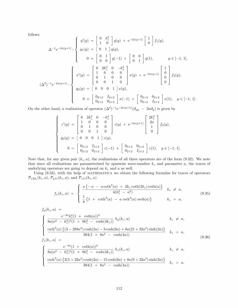
follows
∆−1e−2a(y+1) :
q′(y) =[
0 k2z
1 0
]q(y) + e−2a(y+1)
[10
]f1(y),
g1(y) =[
0 1]q(y),
0 =[
0 10 0
]q(−1) +
[0 00 1
]q(1), y ∈ [−1, 1],
(∆2)−1e−2a(y+1) :
x′(y) =
0 2k2z 0 −k4
z
1 0 0 00 1 0 00 0 1 0
x(y) + e−2a(y+1)
1000
f2(y),
g2(y) =[
0 0 0 1]x(y),
0 =[
02×2 I2×2
02×2 02×2
]x(−1) +
[02×2 02×2
02×2 I2×2
]x(1), y ∈ [−1, 1].
On the other hand, a realization of operator (∆2)−1e−2a(y+1)(∂yy − 2a∂y) is given by
z′(y) =
0 2k2z 0 −k4
z
1 0 0 00 1 0 00 0 1 0
z(y) + e−2a(y+1)
2k2z
2a10
f3(y),
g3(y) =[
0 0 0 1]z(y),
0 =[
02×2 I2×2
02×2 02×2
]z(−1) +
[02×2 02×2
02×2 I2×2
]z(1), y ∈ [−1, 1].
Note that, for any given pair (kz, a), the realizations of all three operators are of the form (9.32). We notethat since all realizations are parameterized by spanwise wave-number kz and parameter a, the traces ofunderlying operators are going to depend on kz and a as well.
Using (9.33), with the help of mathematica we obtain the following formulae for traces of operatorsPx221(kz, a), Py11(kz, a), and Pz11(kz, a)
fx(kz, a) =
a− a − a coth2(a) + 2kz coth(2kz) coth(a)
4(k2
z − a2)kz = a,
181 + coth2(a) − a csch3(a) sech(a)
kz = a,
(9.35)
fy(kz, a) =
e−2ak2z(1 + coth(a))2
8a(a2 − k2z)3(1 + 8k2
z − cosh(4kz))hy(kz, a) kz = a,
csch2(a)(3 − 288a2) cosh(2a) − 3 cosh(6a) + 8a(21 + 32a2) sinh(2a)
384(1 + 8a2 − cosh(4a))
kz = a,
fz(kz, a) =
e−4a(1 + coth(a))2
8a(a2 − k2z)3(1 + 8k2
z − cosh(4kz))hz(kz, a) kz = a,
csch2(a)3(5 + 32a2) cosh(2a) − 15 cosh(6a) + 8a(9 + 32a2) sinh(2a)
384(1 + 8a2 − cosh(4a))
kz = a,
(9.36)
112

where
hy(kz, a) := a cosh(2a)a4 + (akz)2(3 + 8a2) − 16(ak2
z)2 + 8k6
z − a2(a2 + 3k2z) cosh(4kz)
+
kz sinh(2a)−4
(3a4kz − 4a2k3
z + k5z
)+ a2
(3a2 + k2
z
)sinh(4kz)
,
hz(kz, a) := a cosh(2a)−8k8z + 2a6
(1 + 8k2
z
)+ a4
(k2z − 40k4
z
)− a2
(2a4 + (akz)2 + k4
z
)cosh(4kz) +
a2(k4z + 32k6
z
) +
kz sinh(2a)4kz
(−4a6 + 7a4k2
z − 4a2k4z + k6
z
)+ a2
(4a4 − a2k2
z + k4z
)sinh(4kz)
.
Determination of nominal velocity dependent traces
Next, we determine traces of nominal-velocity-dependent operators Ps222 , s = y, z, for both ‘unstructured’and ‘structured’ external excitations in Couette flow. While we are not able to solve for operators Py222 andPz222 explicitly, we are able to express their traces in terms of easily computable series. This is accomplishedat the expense of doing a spectral decomposition of operators L and S (see § 7.1.3 for details).
Determination of trace(Ps222)
We recall that gs, for every s = y, z, is determined by trace(Ps222), where operator Ps222 satisfies
LPs11 + Ps11L = −Ms11, (9.37a)SPs0 + Ps0L = − CpPs11, (9.37b)
SPs222 + Ps222S = − (CpP∗s0 + Ps0C∗
p). (9.37c)
Solutions to (9.37a) and (9.37b) are respectively given by
Ps11 =∫ ∞
0
eLtMs11eLt dt, (9.38a)
Ps0 =∫ ∞
0
eStCpPs11eLt dt, (9.38b)
while trace(Ps222) can be determined as
gs := trace(Ps222) = − 12trace(S−1(CpP∗
s0 + Ps0C∗p)). (9.39)
Combination of (9.38b) and (9.39) yields
gs = −12trace(S−1CpPs11
∫ ∞
0
eLtC∗pe
St dt) − 12trace(S−1Cp
∫ ∞
0
eLtPs11C∗pe
St dt)
=: gs1 + gs2 .
The inherent difficulty is that we cannot determine the above integrals explicitly. However, as we now showthe traces can still be determined by carrying out a spectral decomposition of operators L and S.
In order to evaluate gs1 and gs2 we need the following Lemma.
Lemma 16 Let γnn∈N, ϕnn∈N be the eigenvalues and eigenfunctions of the operator S, then for anytrace class operators F and G
trace(F∫ ∞
0
eLtGeSt dt) = −∑n∈N
⟨ϕn,F(L + γnI)−1Gϕn
⟩.
113

Proof: Let the spectral decompositions of S and L be
S =∑n∈N
γnESn , L =
∑m∈N
λmELm
where ESn and EL
n are the spectral projections of S and L respectively, that is ESn f := 〈ϕn, f〉ϕn and
ELmf := 〈σm, f〉os σm. We can then compute
∫ ∞
0
eLtGeSt dt =∫ ∞
0
∑m∈N
eλmtELm
G∑n∈N
eγntESn
dt
=∑n∈N
∑m∈N
∫ ∞
0
e(λm+γn)t dtELmGES
n
= −∑n∈N
∑m∈N
1(λm + γn)
ELmGES
n
= −∑n∈N
(L + γnI)−1GESn ,
where in the last equation we made a choice to recombine the spectral decomposition of L. Now, thetrace of any operator H can be calculated using any orthonormal basis set ϕii∈N by trace(H) =∑i∈N
〈ϕi,Hϕi〉. Therefore
trace(F∫ ∞
0
eLtGeSt dt) = − trace(F∑n∈N
(L + γnI)−1GESn )
= −∑i∈N
⟨ϕi,F
∑n∈N
(L + γnI)−1GESnϕi
⟩
= −∑n∈N
⟨ϕn,F(L + γnI)−1Gϕn
⟩.
Similarly, by performing a spectral decomposition of L we can express Ps11 as
Ps11 = −∑k∈N
(L + λkI)−1Ms11ELk .
We are now able to express gs1 and gs2 as
gs1 = −12trace(S−1CpPs11
∫ ∞
0
eLtC∗pe
St dt)
= −12
∑n∈N
∑k∈N
⟨ϕn,S−1Cp(L + λkI)−1Ms11E
Lk (L + γnI)−1C∗
pϕn⟩
= −12
∑n∈N
∑k∈N
⟨(L + λkI)−1C∗
pS−1ϕn,Ms11ELk (L + γnI)−1C∗
pϕn⟩os
= −12
∑n∈N
∑k∈N
⟨(L + γnI)−1σk, C∗
pϕn⟩os
⟨(L + λkI)−1C∗
pS−1ϕn,Ms11σk⟩os,
114

and
gs2 = −12trace(S−1Cp
∫ ∞
0
eLtPs11C∗pe
St dt)
= −12
∑n∈N
∑k∈N
⟨ϕn,S−1Cp(L + γnI)−1(L + λkI)−1Ms11E
Lk C∗
pϕn⟩
= −12
∑n∈N
∑k∈N
⟨(L + λkI)−1(L + γnI)−1C∗
pS−1ϕn,Ms11ELk C∗
pϕn⟩os
= −12
∑n∈N
∑k∈N
⟨σk, C∗
pϕn⟩os
⟨(L + λkI)−1(L + γnI)−1C∗
pS−1ϕn,Ms11σk⟩os.
In particular, for Couette flow we have
C∗p = − ikz∆−1 ⇒
C∗pϕn = − ikz
γnϕn,
C∗pS−1ϕn = − ikz
γ2n
ϕn,
which in turn implies
gs1 = −12
∑n∈N
∑k∈N
k2z
γ3n
⟨(L + γnI)−1σk, ϕn
⟩os
⟨(L + λkI)−1ϕn,Ms11σk
⟩os
= −12
∑n∈N
∑k∈N
k2z
γ3n
1(λk + γn)
〈σk, ϕn〉os⟨(L + λkI)−1ϕn,Ms11σk
⟩os
= −12
∑n∈N
∑k∈N
∑m∈N
k2z
γ3n
1(λk + γn)(λm + λk)
〈σk, ϕn〉os 〈σm, ϕn〉os 〈σm,Ms11σk〉os ,
where we arrived at the last equality by performing the spectral decomposition of operator (L + λkI)−1.Similarly,
gs2 = −12
∑n∈N
∑k∈N
k2z
γ3n
〈σk, ϕn〉os⟨(L + λkI)−1(L + γnI)−1ϕn,Ms11σk
⟩os
= −12
∑n∈N
∑k∈N
∑m∈N
k2z
γ3n
1(λm + λk)(λm + γn)
〈σk, ϕn〉os 〈σm, ϕn〉os 〈σm,Ms11σk〉os .
Hence,
gs = −12
∑n,k,m∈N
k2z
γ3n
λk + λm + 2γn(λm + λk)(λk + γn)(λm + γn)
〈σk, ϕn〉os 〈σm, ϕn〉os 〈σm,Ms11σk〉os
= −k2z
2
∑n,k,m∈N
λ1kλ1m(λ1k + λ1m + 2γn)AkAm(nπ)2 cos(p1k) cos(p1m)γ3n(λ1m + λ1k)(λ2
1k − γ2n)(λ2
1m − γ2n)
〈σ1m,Ms11σ1k〉os n − odd,
λ2kλ2m(λ2k + λ2m + 2γn)BkBm(nπ)2 sin(p2k) sin(p2m)γ3n(λ2m + λ2k)(λ2
2k − γ2n)(λ2
2m − γ2n)
〈σ2m,Ms11σ2k〉os n − even,
115

where
p1k tan(p1k) = − kz tanh(kz), λ1k := − (p21k + k2
z), Ak :=
(−λ1k)(
1 +sin(2p1k)
2p1k
)− 12
,
p2k cot(p2k) = kz coth(kz), λ2k := − (p22k + k2
z), Bk :=
(−λ2k)(
1 − sin(2p2k)2p2k
)− 12
,
and
σ1k := Akcos(p1ky) − cos(p1k)cosh(kz)
cosh(kzy),
σ2k := Bksin(p2ky) − sin(p2k)sinh(kz)
sinh(kzy).
Therefore, the remaining task amounts to evaluation of inner products 〈σ1m,Ms11σ1k〉os and 〈σ2m,Ms11σ2k〉osfor s = y, z for both ‘unstructured’ and ‘structured’ disturbances.
Formulae for gy(kz) and gz(kz) in Couette flow
We recall that for ‘unstructured’ disturbances My11 = − k2z∆
−1 and Mz11 = ∆−1∂yy. Thus,
〈σim,My11σik〉os = k2z 〈σim, σik〉2 , 〈σim,Mz11σik〉os = − 〈σim, σ′′
ik〉2 , ∀ i = 1, 2,
where σ′′ik(y) := d2σik(y)/dy2. We evaluate these inner products in mathematica to obtain
〈σ1m,My11σ1k〉os =
k2zAkAm cos(p1k) cos(p1m)(
tanh(kz)kz
+ sech2(kz)) m = k,
k2zA2
k cos2(p1k)(tanh(kz)
kz+ sech2(kz)) − 1
λ1k m = k,
〈σ2m,My11σ2k〉os =
k2zBkBm sin(p2k) sin(p2m)(
coth(kz)kz
− csch2(kz)) m = k,
k2zB2
k sin2(p2k)(coth(kz)
kz− csch2(kz)) − 1
λ2k m = k,
〈σ1m,Mz11σ1k〉os =
− k2zAkAm cos(p1k) cos(p1m)(
tanh(kz)kz
+ sech2(kz)) m = k,
1 − k2zA2
k cos2(p1k)(tanh(kz)
kz+ sech2(kz)) − 1
λ1k m = k,
〈σ2m,Mz11σ2k〉os =
− k2zBkBm sin(p2k) sin(p2m)(
coth(kz)kz
− csch2(kz)) m = k,
1 − k2zB2
k sin2(p2k)(coth(kz)
kz− csch2(kz)) − 1
λ2k m = k.
Formulae for gy(kz, a) and gz(kz, a) in Couette flow
We recall that for ‘structured’ disturbances with ‘pre-modulation’ in y given by (9.10)
My11 = − k2za
2(1 + coth(a))2∆−1e−2a(y+1),
Mz11 = a2(1 + coth(a))2∆−1e−2a(y+1)(∂yy − 2a∂y).
Thus,
〈σim,My11σik〉os = k2za
2(1 + coth(a))2⟨σim, e−2a(y+1)σik
⟩2, ∀ i = 1, 2,
〈σim,Mz11σik〉os = − a2(1 + coth(a))2⟨σim, e−2a(y+1)(σ′′
ik − 2aσ′ik)⟩2, ∀ i = 1, 2,
116

where σ′ik(y) := dσik(y)/dy. The analytical expressions for these inner products can be readily determined
in mathematica.
9.7 Summary
We perform a thorough analysis of the effects of individual inputs (dx, dy, and dz) to the individual outputs (u,v, and w) for the streamwise constant LNS equations. We use this componentwise analysis to derive severalcorollaries that quantify the aggregate effects of: a) inputs in different spatial directions dx, dy, and dz tovelocity vector φ =
[u v w
]T ; b) input vector d :=[dx dy dz
]T to velocity perturbations u, v, andw; and c) forces in all three spatial directions d to all three velocity components φ. We analytically ascertainthat for ‘channel-wide external excitations’, the spanwise and wall-normal forces have the strongest influenceon the velocity field; the impact of these forces is most powerful on the streamwise velocity component. Forexample, we rigorously establish that the singular values of operators from dz and dy to u scale as R2. Onthe other hand, the singular values of operators from all other body force inputs to all other velocity outputsscale as R. Furthermore, for ‘near-wall external excitations’ we demonstrate that dz has, by far, the strongestimpact on the evolution of the velocity field. This observation is consistent with recent numerical work onchannel flow turbulence control using the Lorentz force, where it was concluded that forcing in the spanwisedirection confined within the viscous sub-layer had the strongest effect in suppressing turbulence. We confirmthis observation by analytical derivations that quantify the H2 norms of operators from individual inputs(dx, dy, and dz) to the entire velocity vector φ. Also, we perform a detailed analysis of the dependence of: a)maximal singular values and Hilbert–Schmidt norms on the spanwise wave-number kz and the appropriatelyscaled temporal frequency Ω := ωR; and b) H∞ and H2 on the spanwise wave-number kz. We concludethat for high Reynolds number channel flows small temporal frequency effects dominate the evolution of thevelocity perturbations, and that the most amplified input-output resonances take place at O(1) values of kz.
117

Bibliography
[1] W. C. Reynolds and S. C. Kassinos, “One-point modeling of rapidly deformed homogeneous turbulence,”Proceedings: Mathematical and Physical Sciences, vol. 451, no. 1941, pp. 87–104, 1995.
[2] C. Henoch and J. Stace, “Experimental investigation of a salt water turbulent boundary layer modifiedby an applied streamwise magnetohydrodynamic body force,” Physics of Fluids, vol. 7, no. 6, pp. 1371–1383, 1995.
[3] C. H. Crawford and G. E. Karniadakis, “Reynolds stress analysis of EMHD-controlled wall turbulence.Part I. Streamwise forcing,” Physics of Fluids, vol. 9, no. 3, pp. 788–806, 1997.
[4] T. W. Berger, J. Kim, C. Lee, and J. Lim, “Turbulent boundary layer control utilizing the Lorentzforce,” Physics of Fluids, vol. 12, no. 3, pp. 631–649, 2000.
[5] Y. Du and G. E. Karniadakis, “Suppressing wall turbulence by means of a transverse traveling wave,”Science, vol. 288, pp. 1230–1234, 2000.
[6] Y. Du, V. Symeonidis, and G. E. Karniadakis, “Drag reduction in wall-bounded turbulence via atransverse travelling wave,” J. Fluid Mech., vol. 457, pp. 1–34, 2002.
[7] L. H. Gustavsson, “Energy growth of three-dimensional disturbances in plane Poiseuille flow,” J. FluidMech., vol. 98, p. 149, 1991.
[8] M. T. Landahl, “Wave breakdown and turbulence,” SIAM J. Appl. Math., vol. 28, pp. 735–756, 1975.
[9] J. Kim and J. Lim, “A linear process in wall-bounded turbulent shear flows,” Physics of Fluids, vol. 12,no. 8, pp. 1885–1888, 2000.
[10] G. Kreiss, A. Lundbladh, , and D. S. Henningson, “Bounds for threshold amplitudes in subcritical shearflows,” J. Fluid Mech., vol. 270, pp. 175–198, 1994.
[11] B. Bamieh and M. Dahleh, “Energy amplification in channel flows with stochastic excitation,” Physicsof Fluids, vol. 13, no. 11, pp. 3258–3269, 2001.
118

Chapter 10
Spatio-temporal impulse responses ofthe linearized Navier-Stokes equationsin channel flows
In this chapter, we carry input-output analysis of the LNS equations in channel flows further by investigatingtheir spatio-temporal impulse responses. The motivation for this is twofold. First, the response to any forcingfield is the superposition of shifted (spatially and temporally) family of impulse responses. Thus, the impulseresponses contain qualitatively all the properties of the dynamical response. Second, these responses turnout to be closely related to numerical and experimental observations of early stages of turbulent spots. Theybear remarkable qualitative resemblance to the turbulent spots, in terms of the ‘arrow-head’ shape, thestreaky structures, and the cross-contamination phenomena as the spots grow. This resemblance is onlyqualitative, as other features of turbulent spots are not represented in the responses we compute. Our mainpoint however is that for a full understanding of the rich dynamics of the LNS equations one must lookat all of these responses. The features of the impulse responses are difficult to extract from the frequencyresponses (cf. chapters 8 and 9), and are certainly not obvious from the classical modal analysis of the LNSequations.
Several researchers have heretofore reported numerically determined responses of the NS and LNS equa-tions in channel flows. Henningson & Kim [1] studied the turbulence characteristics inside the turbulentspot by performing Direct Numerical Simulations (DNS) in Poiseuille flow with R = 1500. The initial con-dition assumed a form of a double vortex. The authors found significant agreement between their resultsand experimental observations and concluded that the fully developed turbulent spot does not depend onthe initial conditions. Henningson, Lundbladh & Johansson [2] studied the early stages of laminar-turbulenttransition by analyzing the development of localized disturbances in Poiseuille and boundary layer flows. Theobtained results were based on both the DNS and the analysis of the LNS equations. The Reynolds numberin Poiseuille flow was set to 3000, and the flow was initialized by two pairs of counter-rotating vortices.The authors reported the dominance of streamwise elongated structures and underlined the importance ofa linear three-dimensional lift-up mechanism [3, 4]. Li & Widnall [5] computed the steady-state responseof the forced LNS equations in an undertaking to model the structure around turbulent spot in Poiseuilleflow. The forces into the LNS equations were introduced to account for the Reynolds stresses resulting fromthe regions of small-scale turbulence. The authors found qualitative agreement between the oblique wavessurrounding the spot and experimental results of [6]. Lundbladh & Johansson [7] performed the DNS of theplane Couette flow for various Reynolds numbers in the range between 300 and 1500. The flow was kickedoff by an initial condition in the form of four pairs of counter-rotating vortices and transition was observedto take place at R ≈ 375. This value is very close to the lowest Reynolds number for which turbulence canbe experimentally maintained [8, 9].
The numerical computations that we perform in this chapter are focused on earlier stages of transitionprocess in Poiseuille flow initiated by the linearized dynamics. One important distinction between our
119

results and previously published studies is in the way the flow field is computed. Most of the aforementionedreferences have analyzed the databases obtained as responses to favorably constructed initial conditions. We,on the other hand, study the response of the forced LNS equations to zero initial conditions. The externalexcitation is chosen in the form of an impulse located in the vicinity of the lower wall. This particular inputshape is selected to ‘mimic’ the conditions under which the ‘natural transition’ is observed in laboratory [10].We find that our results have some of the qualitative features of early stages of turbulent spot developmentobserved in the previously reported experimental and numerical Poiseuille flow investigations.
Our presentation is organized as follows: in § 10.1 we briefly review the notion of the spatio-temporalimpulse response of the LNS equations (see Chapter 2 for background material). In § 10.2, we study thespatio-temporal impulse responses of the LNS in subcritical Poiseuille flow with R = 2000. We end ourpresentation with some concluding remarks in § 10.3.
10.1 Preliminaries
From Chapter 7, we recall that a model of the LNS system with impulsive external excitations (7.22) is givenby
∂tψ(kx, y, kz, t) = [A(kx, kz)ψ(kx, kz, t)](y) + F(kx, y, kz)δ(t),φ(kx, y, kz, t) = [C(kx, kz)ψ(kx, kz, t)](y),
where, for notational convenience, we omit the ‘caret symbol’ to denote Fourier transformed signals andoperators. The temporal Dirac delta function is given by δ(t). On the other hand, for any (kx, kz), F(kx, y, kz)represents a multiplication operator in y
F(kx, y, kz) := Fx(kx, y, kz) + Fy(kx, y, kz) + Fz(kx, y, kz),
Fx =
[−ikx∆−1f ′x0
ikzfx0
], Fy =
[−(k2
x + k2z)∆
−1fy0
0
], Fz =
[−ikz∆−1f ′z0−ikxfz0
],
and f0(y) :=[fx0(y) fy0(y) fz0(y)
]T denotes an arbitrary function of the wall-normal coordinate.The solution of system (7.22) in the presence of zero initial conditions is, for any quadruple (kx, y, kz, t),
determined byφ(kx, y, kz, t) = φx(kx, y, kz, t) + φy(kx, y, kz, t) + φz(kx, y, kz, t),
whereφs(kx, y, kz, t) :=
[us(kx, y, kz, t) vs(kx, y, kz, t) ws(kx, y, kz, t)
]Trepresents the system’s response to the forcing applied in a certain spatial direction (for s = x streamwise,for s = y wall-normal, or for s = z spanwise):
us(kx, y, kz, t)
vs(kx, y, kz, t)
ws(kx, y, kz, t)
= [C(kx, kz)ψs(kx, kz, t)] (y)
=[C(kx, kz)eA(kx,kz)tFs(kx, kz)
](y) =: [Gs(kx, kz, t)] (y)
=
[Cu(kx, kz)eA(kx,kz)tFs(kx, kz)
](y)[
Cv(kx, kz)eA(kx,kz)tFs(kx, kz)](y)[
Cw(kx, kz)eA(kx,kz)tFs(kx, kz)](y)
=:
[Gus(kx, kz, t)] (y)[Gvs(kx, kz, t)] (y)[Gws(kx, kz, t)] (y)
.
Operators Grs, r = u, v, w; s = x, y, z, contain a large amount of information about the dynamicalbehavior of system (7.22). In particular, application of an inverse spatial Fourier transform yields solutionsthat can be visualized in the physical space. In addition to that, some intuition can be gained by analyzing
120

quantities that aggregate the effects of dynamics in a certain spatial and/or temporal direction. For example,the wall-normal dynamics can be comprised by computing the Hilbert–Schmidt norm of operator Gs[
‖Gs‖2HS
](kx, kz, t) := trace(G∗
s (kx, kz, t)Gs(kx, kz, t)) = trace(Gs(kx, kz, t)G∗s (kx, kz, t))
= trace(F∗s(kx, kz)e
A∗(kx,kz)tC∗(kx, kz)C(kx, kz)eA(kx,kz)tFs(kx, kz))
= trace(C(kx, kz)eA(kx,kz)tFs(kx, kz)F∗s(kx, kz)e
A∗(kx,kz)tC∗(kx, kz)).
(10.2)
It can be shown that, for example,[‖Gx‖2
HS
](kx, kz, t) represents the kinetic energy density of a harmonic
perturbation in the presence of the streamwise forcing. This quantity is commonly used as a measure ofthe velocity field perturbations [11]. The kinetic energy density can be further averaged over the remainingspatial directions or time:
[‖Gs‖2
2
](kx, kz) :=
∫ ∞
0
[‖Gs‖2
HS
](kx, kz, t) dt, (10.3)
[‖Gs‖2
2
](kx, t) :=
12π
∫ ∞
−∞
[‖Gs‖2
HS
](kx, kz, t) dkz, (10.4)
and so on. The quantity defined by (10.3) can be also interpreted as the H2 norm of system (7.22) in thepresence of an external excitation applied in the spatial direction s, s = x, y, z [12].
We remind the reader that, for stable systems, the H2 norm can be determined using the solutions ofthe operator algebraic Lyapunov equations (see Chapter 2)
A∗(kx, kz)Y(kx, kz) + Y(kx, kz)A(kx, kz) = −C∗(kx, kz)C(kx, kz),
A(kx, kz)Xs(kx, kz) + Xs(kx, kz)A∗(kx, kz) = −Fs(kx, kz)F∗s(kx, kz),
where A∗, F∗s, and C∗ respectively represent adjoints of operators A, Fs, and C. The H2 norm is then
computed from either of the following two expressions[‖Gs‖2
2
](kx, kz) = traceF∗
s(kx, kz)Y(kx, kz)Fs(kx, kz) = traceC(kx, kz)Xs(kx, kz)C∗(kx, kz).
The input distribution in the wall-normal direction can be chosen in a number of different ways. Sinceour primary objective is computation of the spatio-temporal impulse responses we would like to introducean input that is a delta function in y as well. Because of this, we choose fs0 of the form
fs0(y) = δ(y − y0), s = x, y, z, −1 < y0 < 1.
However, since we have to approximate the equations in y numerically, the desired choice of fs0 has to beapproximated with something that is similar to the Dirac function. Using an alternative definition of thedelta function
δ(y − y0) := limε→0+
12√πε
e−
(y − y0)2
4ε ,
we propose the following choice for fs0(y)
fs0(y) =1
2√πε
e−
(y − y0)2
4ε , ε > 0.
Figure 10.1 shows fs0(y) for y0 = −0.9, and ε = 1/2000. Clearly, the shape of the disturbance is not anideal impulse in the y direction, but is an approximation that is good enough to capture the phenomena weare interested in.
The mathematical considerations required for a precise description of the above operators and theiradjoints are included in § 7.1.2. Section 10.2 contains the description of numerical results obtained by
121

−1 −0.5 0 0.5 1
0
2
4
6
8
10
12
y
d s0(y
)
Figure 10.1: Forcing distribution in the wall-normal direction for y0 = −0.9, and ε = 1/2000.
computing the impulse response of the LNS equations in subcritical Poiseuille flow with R = 2000.
10.2 Spatio-temporal impulse responses in Poiseuille flow withR = 2000
In this section, we study the spatio-temporal impulse responses of the LNS equations in plane Poiseuille flowwith R = 2000. All computations are done for R = 2000, with 40 v and ωy basis functions (N = M = 39).Both streamwise constant (kx = 0) and full three-dimensional perturbations are considered. The numericalcomputations for these two cases are performed by gridding in the wave-number space and then applying aninverse Fourier transform to obtain the solutions in the physical space. The streamwise constant calculationsare performed using 1024 linearly spaced Fourier modes in the z-direction with kzmin := −200, kzmax :=200. The number of grid points in the full three-dimensional computations was different for earlier andlater time instants. For t = 5, 10, 15, 20, computations are performed with 256 × 256 linearly spaced gridpoints in the (kx, kz)–plane, with kxmin := −20, kxmax := 19.84375 and kzmin := −30, kzmax := 30.For later times (t = 40, 80, 120, 160) the wave-number plane was divided into 512 × 256 linearly spacedpoints with kxmin := −5, kxmax := 4.98046875 and kzmin := −18, kzmax := 18. Only half the numberof modes in the spanwise direction are used due to symmetry properties. The ODEs for spectral coefficientsare solved in matlab using the numerical scheme described in § 7.2.
10.2.1 Impulse responses for streamwise independent perturbations
Figure 10.2 illustrates the kz–parameterized H2 norms of operators Gs, s = x, y, z, for streamwise indepen-dent perturbations. The shown quantities are obtained based on solutions of the corresponding Lyapunovequations presented in § 10.1. We notice characteristic peaks in the middle and right plots. On the other hand,[‖Gx‖2] (kz) decays monotonically as kz increases, and achieves much smaller values than both [‖Gy‖2] (kz)and [‖Gz‖2] (kz). Also, we observe that the spanwise forcing experiences almost an order of magnitude largeramplification than the wall-normal forcing.
The kinetic energy density of streamwise constant perturbations, as a function of time, is shown inFigure 10.3. The kz–dependence is averaged according to (10.4). Clearly, the kinetic energy density decaysmonotonically in the presence of dx. On the other hand, when either dy or dz is introduced the kineticenergy density experiences transient amplification before eventual decay. We also observe that [‖Gy‖2] (t)peaks sooner than [‖Gz‖2] (t). Furthermore, the former quantity has much bigger rate of decay than thelatter. These facts together with the results shown in Figure 10.2 imply that, at kx = 0, the spatio-temporalimpulsive forcing located in the vicinity of the lower wall is, by far, most effective when applied in thespanwise direction. This is in agreement with our results presented in § 9.4 where, for the streamwiseconstant perturbations, we analytically established that the spanwise near-wall forcing has the strongesteffect on the evolution of the velocity components.
The spatio-temporal impulse response to the z–direction force at kx = 0 is shown in Figure 10.4. In
122

0 5 10 154
5
6
7
8
9
kz
[||G
x|| 2] (k
z)
0 5 10 150
5
10
15
20
25
30
35
40
45
kz
[||G
y|| 2] (k
z)0 5 10 15
0
50
100
150
200
250
300
kz
[||G
z|| 2] (k
z)
Figure 10.2: Plots of [‖Gx‖2] (kz), [‖Gy‖2] (kz), and [‖Gz‖2] (kz) for streamwise constant perturbations. Forc-ing of the form ds = fs0(y)δ(z, t) is introduced, where fs0(y), for every s = x, y, z, is shown in Figure 10.1.
50 100 150 2000
5
10
15
20
t
[||G
s|| 2] (t
)
50 100 150 2000
0.2
0.4
0.6
0.8
1
t
[||G
s|| 2] (t
)/m
ax([
||Gs|| 2]
(t))
Figure 10.3: Plots of [‖Gx‖2] (t) (blue), [‖Gy‖2] (t) (green), and [‖Gz‖2] (t) (red) for streamwise constantperturbations. Forcing of the form ds = fs0(y)δ(z, t) is introduced, where fs0(y), for every s = x, y, z, isshown in Figure 10.1.
123

Figure 10.4: Streamwise velocity (pseudo-color plots) and stream-function (contour plots) perturbationdevelopment for streamwise constant perturbations at: t = 5 s (top left), t = 20 s (top right), t = 100 s(bottom left), and t = 200 s (bottom right). Forcing of the form dx = dy ≡ 0, dz = fz0(y)δ(z, t) isintroduced, where fz0(y) is shown in Figure 10.1. Red color represents high speed streak, and blue colorrepresents low speed streak. The vortex between the streaks is counter clockwise rotating.
particular, the pseudo-color plots of the streamwise velocity perturbation and contour plots of the stream-function in the (z, y)–plane are shown. These plots reveal the presence of a counter clockwise rotating vortex,a low speed streak, and a high speed streak. Clearly, the vortex is positioned between the high speed and thelow speed streaks. We note that the streaks magnitude increases in the early stages of their development andafterwards it slowly decreases. The streaks also spread in both the wall-normal and the spanwise directionsas time goes on. These facts explain the transient energy amplification and consequent slow rate of decayobserved in Figure 10.3. Furthermore, the dominant structures are confined to the region between the lowerwall and the channel’s centerline, whereas a much weaker pair of streaks develops in the upper part of thechannel. This can be attributed to the fact that the shape of the input in y is approximated by an impulselocated near the lower wall. The full three-dimensional computations, that we discuss in § 10.2.2, reveal theexistence of alternating regions of high and low velocities in the spanwise directions, the feature not observedin the computations performed at kx = 0.
10.2.2 Impulse responses for full three-dimensional perturbations
Figure 10.5 shows the H2 norm of three-dimensional perturbations, as a function of both kx and kz. Thequantities defined by (10.3) are determined based on solutions of the corresponding Lyapunov equations,with 50× 90 grid points in the wave-number space (kx, kz). These points are chosen in the logarithmic scalewith kxmin := 10−4, kxmax := 3.02 and kzmin := 10−2, kzmax := 15.84. Clearly, both [‖Gy‖2] (kx, kz)and [‖Gz‖2] (kx, kz) achieve largest values for a relatively broad range of streamwise wave-numbers. Theglobal maxima of these two quantities occur at (kx = 0, kz = O(1)). On the other hand, in the left plot
124

log10([‖Gx‖2] (kx, kz)): log10([‖Gy‖2] (kx, kz)): log10([‖Gz‖2] (kx, kz)):
Figure 10.5: Plots of [‖Gx‖2] (kx, kz), [‖Gy‖2] (kx, kz), and [‖Gz‖2] (kx, kz). Forcing of the form ds =fs0(y)δ(x, z, t) is introduced, where fs0(y), for every s = x, y, z, is shown in Figure 10.1.
the maximum takes place in the narrow region located in the vicinity of (kx ≈ 1, kz ≈ 1). We also observea distinct local peak at kz = 0 on the same plot, which corresponds to the TS wave. Furthermore, the H2
norm achieves the largest values when dz is introduced, which is in agreement with the previously discussedkx = 0 results. This further illustrates that a forcing confined to the near-wall region is much more efficientwhen applied in the spanwise direction than in the other two spatial directions.
In the remainder of this section, we respectively investigate the spatio-temporal impulse responses of theLNS system for forces applied in all three spatial directions.
The three-dimensional isosurface plots of u, obtained in the presence of an impulsive spanwise forcing,are shown in Figure 10.6. Our results illustrate the propagation of the streamwise velocity perturbationas a function of both time and spatial coordinates. It seems that perturbation spreads quickly to theupper part of the channel. Further, it is noteworthy that the early stages of perturbation development arecharacterized by the streamwise variations in the velocity profile. These streamwise variations become lessprominent as time goes on. For larger times the perturbation evolution is dominated by the structureselongated in the direction of a nominal flow. These streamwise streaky structures are usually identified inthe experimental investigations related to the laminar-turbulent transition in both channel [6, 10, 13] andboundary layer flows [14,15]. We also observe two well developed regions almost antisymmetric with respectto the horizontal plane y = 0 that divides the computational domain into two parts of equal size. The reasonfor their existence is shear, which, in Poiseuille flow, is equal to zero in the middle of the channel and growslinearly in the same fashion as one approaches either the lower or the upper wall.
Figure 10.7 shows the pseudo-color plots of the streamwise velocity perturbation profile in the horizontalplane y ≈ 0.68 at eight different time instants. These results are obtained as a response to an impulsivespanwise forcing. The first four plots indicate the presence of streamwise varying structures in the earlystages of perturbation development. On the other hand, the last four plots have the rather characteristicdownstream pointing arrow-head shapes, with streamwise streaky structures ubiquitous in experimentalstudies of both channel [6, 10, 13] and boundary layer flows [14, 15]. We also note that the magnitude of uincreases in the early stages of perturbation development and afterwards it slowly decreases. Furthermore,all plots clearly illustrate the spanwise cross-contamination and perturbation development in both x andz as time progresses. As previously mentioned, the appearance of alternating regions of high and lowvelocities in the spanwise direction is not a feature of the streamwise constant perturbations. Rather, it is aphenomenon that occurs only when the full three-dimensional perturbations are considered. It seems thatthe absence of the downstream convection at kx = 0 prevents spanwise cross-contamination. Furthermore,for the streamwise constant perturbations, ωx depends only on v (cf. (7.11)), which significantly reduces theproduction of the streamwise vorticity in this case. This may serve as yet another explanation with regardto why the alternating regions of high and low speed streaks are observed only in the full three-dimensionalcomputations. However, we remark that the streaks do not propagate in the spanwise direction. Thespanwise spreading of the streamwise perturbation structure is due to the creation of new weaker streaks,rather than the propagation of the existing ones [10].
125

Figure 10.6: Streamwise velocity perturbation isosurface plots at: t = 5 s (first row left), t = 10 s (firstrow right), t = 15 s (second row left), t = 20 s (second row right), t = 40 s (third row left), t = 80 s (thirdrow right), t = 120 s (fourth row left), and t = 160 s (fourth row right). Forcing of the form dx = dy ≡ 0,dz = fz0(y)δ(x, z, t) is introduced, where fz0(y) is shown in Figure 10.1. Red color represents regions of highvelocity, and green color represents regions of low velocity. Isosurfaces are taken at ±10−3.
126

Figure 10.7: Streamwise velocity perturbation pseudo-color plots in the horizontal plane y ≈ 0.68 at: t = 5 s(first row left), t = 10 s (first row right), t = 15 s (second row left), t = 20 s (second row right), t = 40 s(third row left), t = 80 s (third row right), t = 120 s (fourth row left), and t = 160 s (fourth row right).Forcing of the form dx = dy ≡ 0, dz = fz0(y)δ(x, z, t) is introduced, where fz0(y) is shown in Figure 10.1.Hot colors represent regions of high velocity, and cold colors represent regions of low velocity.
127
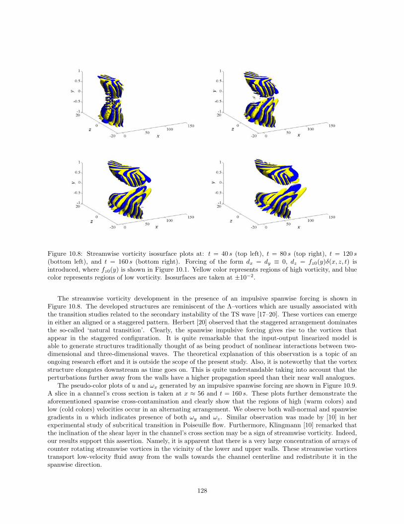
Figure 10.8: Streamwise vorticity isosurface plots at: t = 40 s (top left), t = 80 s (top right), t = 120 s(bottom left), and t = 160 s (bottom right). Forcing of the form dx = dy ≡ 0, dz = fz0(y)δ(x, z, t) isintroduced, where fz0(y) is shown in Figure 10.1. Yellow color represents regions of high vorticity, and bluecolor represents regions of low vorticity. Isosurfaces are taken at ±10−2.
The streamwise vorticity development in the presence of an impulsive spanwise forcing is shown inFigure 10.8. The developed structures are reminiscent of the Λ–vortices which are usually associated withthe transition studies related to the secondary instability of the TS wave [17–20]. These vortices can emergein either an aligned or a staggered pattern. Herbert [20] observed that the staggered arrangement dominatesthe so-called ‘natural transition’. Clearly, the spanwise impulsive forcing gives rise to the vortices thatappear in the staggered configuration. It is quite remarkable that the input-output linearized model isable to generate structures traditionally thought of as being product of nonlinear interactions between two-dimensional and three-dimensional waves. The theoretical explanation of this observation is a topic of anongoing research effort and it is outside the scope of the present study. Also, it is noteworthy that the vortexstructure elongates downstream as time goes on. This is quite understandable taking into account that theperturbations further away from the walls have a higher propagation speed than their near wall analogues.
The pseudo-color plots of u and ωx generated by an impulsive spanwise forcing are shown in Figure 10.9.A slice in a channel’s cross section is taken at x ≈ 56 and t = 160 s. These plots further demonstrate theaforementioned spanwise cross-contamination and clearly show that the regions of high (warm colors) andlow (cold colors) velocities occur in an alternating arrangement. We observe both wall-normal and spanwisegradients in u which indicates presence of both ωy and ωz. Similar observation was made by [10] in herexperimental study of subcritical transition in Poiseuille flow. Furthermore, Klingmann [10] remarked thatthe inclination of the shear layer in the channel’s cross section may be a sign of streamwise vorticity. Indeed,our results support this assertion. Namely, it is apparent that there is a very large concentration of arrays ofcounter rotating streamwise vortices in the vicinity of the lower and upper walls. These streamwise vorticestransport low-velocity fluid away from the walls towards the channel centerline and redistribute it in thespanwise direction.
128

Figure 10.9: Pseudo-color plots of the streamwise velocity (left) and vorticity (right) perturbation profiles ina cross section of the channel at x ≈ 56 and t = 160 s. Forcing of the form dx = dy ≡ 0, dz = fz0(y)δ(x, z, t)is introduced, where fz0(y) is shown in Figure 10.1.
The three-dimensional isosurface plots and the pseudo-color plots of u in the horizontal plane at y ≈ 0.68are respectively illustrated in Figures 10.10 and 10.11. The shown results represent a response to an impulsivewall-normal forcing. The early stages of perturbation development are dominated by the oblique waves, asfor the ‘dz impulse response computations’. These streamwise varying structures can be also observed inthe later phases of spot evolution, even though the streamwise elongated effects become dominant for largertimes. The three-dimensional isosurface plots indicate the presence of two forward pointing arrowhead-shaped shear layers with ‘legs’ that extend in the upstream direction towards the walls, as in the case of the‘dz impulse response results’. Remarkably, this shape of disturbance was postulated by Klingmann [10] inher analysis of the streamwise velocity perturbation contour plots in the (y, z)–plane. These contour plotswere obtained experimentally by essentially determining the response of the subcritical Poiseuille flow to animpulsive y–direction forcing. A sequence of measurements was made at different time instants by traversinga single hot-wire probe in a channel’s cross section in both wall-normal and spanwise directions. Basedon our two dimensional pseudo-color plots, it seems that the entire structure elongates at approximately aconstant rate during its downstream propagation. Landahl [4] theoretically predicted that the streamwiseextent of the disturbed region grows linearly with time for all parallel inviscid shear flows. Furthermore, thenew streaks of fairly weak magnitude appear on the spanwise edges of the spot as it travels downstream.
The streamwise forcing impulse response results are shown in Figures 10.12 and 10.13, where we respec-tively illustrate the three-dimensional isosurface plots, and the pseudo-color plots of u in the horizontal planeat y ≈ 0.68. The presence of oblique waves is much more prominent here than in the ‘dy and dz impulseresponse computations’. Even though the perturbation elongates as time goes on and shapes into the char-acteristic arrow-head downstream-oriented structure, the streamwise variations dominate its development.From the left plot in Figure 10.5, we recall that the peaks of the H2 norm in the presence of dx take placeat O(1) values of both kx and kz. This fact may serve as an explanation for fairly rich streamwise behaviorwhen linearized dynamics are forced by dx.
All results shown in this subsection illustrate the ability of the linearized model subject to externalforces to generate, at least qualitatively, structures (oblique waves, streamwise vortices and streaks) usuallyobserved in experimental laminar-turbulent transition investigation in wall-bounded shear flows [6,10,13–15].
10.3 Summary
We consider the NS equations linearized about a parallel channel flow of the form U(y) = 1−y2 in the presenceof spatially distributed three-dimensional body forces. We carry out an input-output analysis to investigatethe dependence of various velocity and vorticity ‘outputs’ on the various impulsive body force ‘inputs’. Thespatio-temporal impulse responses of the LNS equations in channel flows, to our knowledge, have not been
129

Figure 10.10: Streamwise velocity perturbation isosurface plot at: t = 40 s (top left), t = 80 s (top right),t = 120 s (bottom left), and t = 160 s (bottom right). Forcing of the form dx = dz ≡ 0, dy = fy0(y)δ(x, z, t)is introduced, where fy0(y) is shown in Figure 10.1. Red color represents regions of high velocity, and greencolor represents regions of low velocity. Isosurfaces are taken at ±2 × 10⁻⁴.
130
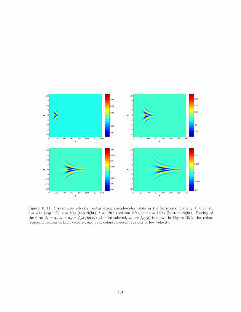
Figure 10.11: Streamwise velocity perturbation pseudo-color plots in the horizontal plane y ≈ 0.68 at:t = 40 s (top left), t = 80 s (top right), t = 120 s (bottom left), and t = 160 s (bottom right). Forcing ofthe form dx = dz ≡ 0, dy = fy0(y)δ(x, z, t) is introduced, where fy0(y) is shown in Figure 10.1. Hot colorsrepresent regions of high velocity, and cold colors represent regions of low velocity.
131

Figure 10.12: Streamwise velocity perturbation isosurface plots at: t = 40 s (top left), t = 80 s (top right),t = 120 s (bottom left), and t = 160 s (bottom right). Forcing of the form dy = dz ≡ 0, dx = fx0(y)δ(x, z, t)is introduced, where fx0(y) is shown in Figure 10.1. Red color represents regions of high velocity, and greencolor represents regions of low velocity. Isosurfaces are taken at ±2 × 10⁻⁴.
132

Figure 10.13: Streamwise velocity perturbation pseudo-color plots in the horizontal plane y ≈ 0.68 at:t = 40 s (top left), t = 80 s (top right), t = 120 s (bottom left), and t = 160 s (bottom right). Forcing ofthe form dy = dz ≡ 0, dx = fx0(y)δ(x, z, t) is introduced, where fx0(y) is shown in Figure 10.1. Hot colorsrepresent regions of high velocity, and cold colors represent regions of low velocity.
133

previously reported in the literature. We show that the flow response to spatio-temporal impulsive inputsforms spot-like structures with an arrow-head shape that elongates as it convects downstream. These spotsare made up of alternating and staggered regions of high and low speed velocity streaks with counter-rotatingvortices between them. The identified structures are inclined with respect to the wall and their inclinationchanges as the spot grows or decays. The spots bear a qualitative similarity to structures observed in fullynonlinear initial value simulations in channel flows, while the streaky and vortical structures within themare qualitatively similar to those observed in turbulent boundary layers. As an argument for the need forthis kind of impulse response analysis of the linearized equations, we point out that such structures arepractically impossible to observe from a purely modal analysis of the LNS equations.
As a final remark we point out that the LNS equations appear to have very complex dynamics thatcan be explored in various ways. Significantly different flow structures are induced by exciting the flowin different manners. It has long been recognized that background excitation and uncertainty significantlyimpact the flow structures observed in channel flow and boundary layer experiments, and that full directnumerical simulations are capable of reproducing this rich behavior. We observe here that even the linearizedequations appear to contain much of that behavior.
134

Bibliography
[1] D. S. Henningson and J. Kim, “On turbulent spots in plane Poiseuille flow,” J. Fluid Mech., vol. 228,pp. 183–205, 1991.
[2] D. S. Henningson, A. Lundbladh, and A. V. Johansson, “A mechanism for bypass transition fromlocalized disturbances in wall-bounded shear flows,” J. Fluid Mech., vol. 250, pp. 169–207, 1993.
[3] M. T. Landahl, “Wave breakdown and turbulence,” SIAM J. Appl. Math., vol. 28, pp. 735–756, 1975.
[4] ——, “A note on an algebraic instability of inviscid parallel shear flows,” J. Fluid Mech., vol. 98, pp.243–251, 1980.
[5] F. Li and S. E. Widnall, “Wave patterns in plane Poiseuille flow created by concentrated disturbances,”J. Fluid Mech., vol. 208, pp. 639–656, 1989.
[6] D. R. Carlson, S. E. Widnall, and M. F. Peeters, “A flow-visualization study of transition in planePoiseuille flow,” J. Fluid Mech., vol. 121, pp. 487–505, 1982.
[7] A. Lundbladh and A. V. Johansson, “Direct simulation of turbulent spots in plane Couette flow,” J.Fluid Mech., vol. 229, pp. 499–516, 1991.
[8] N. Tillmark and P. H. Alfredsson, “Experiments on transition in plane Couette flow,” J. Fluid Mech.,vol. 235, pp. 89–102, 1992.
[9] O. Dauchot and F. Daviaud, “Finite amplitude perturbation and spots growth mechanism in planeCouette flow,” Physics of Fluids, vol. 7, no. 2, pp. 335–343, 1995.
[10] B. G. B. Klingmann, “On transition due to three-dimensional disturbances in plane Poiseuille flow,” J.Fluid Mech., vol. 240, pp. 167–195, 1992.
[11] K. M. Butler and B. F. Farrell, “Three-dimensional optimal perturbations in viscous shear flow,” Physicsof Fluids A, vol. 4, p. 1637, 1992.
[12] K. Zhou, J. C. Doyle, and K. Glover, Robust and Optimal Control. Prentice Hall, 1996.
[13] F. Alavyoon, D. S. Henningson, and P. H. Alfredsson, “Turbulent spots in plane Poiseuille flow - flowvisualization,” Physics of Fluids, vol. 29, no. 4, pp. 1328–1331, 1986.
[14] F. W. Chambers and A. S. W. Thomas, “Turbulent spots, wave packets, and growth,” Physics of Fluids,vol. 26, no. 5, pp. 1160–1162, 1983.
[15] M. Matsubara and P. H. Alfredsson, “Disturbance growth in boundary layers subjected to free-streamturbulence,” J. Fluid Mech., vol. 430, pp. 149–168, 2001.
[16] B. Bamieh and M. Dahleh, “Energy amplification in channel flows with stochastic excitation,” Physicsof Fluids, vol. 13, no. 11, pp. 3258–3269, 2001.
[17] P. S. Klebanoff, K. D. Tidstrom, and L. M. Sargent, “The three-dimensional nature of boundary-layerinstability,” J. Fluid Mech., vol. 12, pp. 1–34, 1962.
135

[18] V. V. Kozlov and M. P. Ramazanov, “Development of finite-amplitude disturbances in Poiseuille flow,”J. Fluid Mech., vol. 147, pp. 149–157, 1984.
[19] B. J. Bayly, S. A. Orszag, and T. Herbert, “Instability mechanisms in shear flow transition,” Ann. Rev.Fluid Mech., vol. 20, pp. 359–391, 1988.
[20] T. Herbert, “Secondary instability of boundary layers,” Ann. Rev. Fluid Mech., vol. 20, pp. 487–526,1988.
136

Chapter 11
Conclusions and future directions
Conclusions
In contrast to the large body of work by physicists and engineers with expertise in fluid mechanics, systemtheoreticians have made minimal contributions to the area of flow modeling and control. As this thesisdemonstrates, a number of issues in fluid mechanics can be addressed effectively using system theoreticaltools. For example, we have employed input-output system analysis to:
• Unravel new mechanisms for subcritical transition.
• Compare roles of TS waves, oblique waves, and streamwise vortices and streaks in subcritical transition.
• Quantify effectiveness of forcing components.
• Quantify energy content of velocity components.
• Compare roles of unstable and ‘non-normal’ modes in supercritical flows.
• Study spatio-temporal impulse responses of the LNS equations in Poiseuille flow.
Thus, we have demonstrated that modern control theory can be very effective in advancing a classical field.On the other hand, system theoreticians can benefit tremendously from being exposed to fluid mechanicalproblems, because these physically relevant problems pose new theoretical challenges that traditionally havenot been addressed in the control’s literature. In view of this, an interdisciplinary research effort is necessaryto facilitate a transfer of knowledge from fluid mechanics to control and vice versa.
My goal is to continue development of systematic analysis and design procedures for understanding andcontrolling transitional and turbulent shear flows, using both system theoretical and fluid mechanical tools.Several topics for future research are given below.
Future directions
Modeling flow statistics using the LNS equations. In [1], we addressed the problem of modelingdisturbances in the LNS equations by testing the validity−in quantitative sense−of a stochastically excitedversion of the linearized model. We developed a model for second order statistics of turbulent channelflow using an associated linear stochastically forced input-output system. Our results showed that certainportions of DNS-based flow statistics can be closely matched by the appropriate choice of input forcingcovariance. This was done in an ad hoc fashion using a variety of excitation force correlations and showingthe dependence of the velocity field statistics on them. We intend to develop a precise methodology fordetermination of external excitation statistics to guarantee matching DNS-based data in some optimal (e.g.,least-squared) sense.
137

The motivation for this problem is twofold: a) model validation of the stochastically excited LNS equa-tions, and b) proper weight selection in optimal control problems for drag reduction. We plan to use theinput correlations determined in this way as a disturbance model in an H2-optimal control problem. Asis well known, proper weight selection can dramatically alter control performance when the controller isin feedback with the actual nonlinear system. It is therefore anticipated that an H2 controller designedusing these weights will have superior performance to a controller designed without an accurate disturbancemodel. Furthermore, it is expected that this controller will lead to successful turbulence suppression withlinear controllers in high Reynolds number flows.
Active and passive control of transition and turbulence. The use of Micro-Electro-MechanicalSystems (MEMS) devices for flow actuation and sensing is likely to revolutionize active and passive flowcontrol in wall-bounded shear flows (e.g., boundary layer, pipe, and channel flows). This, however, wouldrequire a fully-integrated system design that accounts for the complex dynamics of flow phenomena. A workreported in this dissertation represents a step in that direction.
In this thesis, we have developed mathematical models that rigorously account for uncertain body forces.Also, we have initiated development of models that quantify the effects of both dynamical uncertaintiesand wall texture on flow perturbations. We plan to use these models as the basis for new control designs,including active (e.g., H2 and H∞) and passive control strategies for drag reduction.
Passive flow control is a promising technology for implementation. Examples of passive control strategiesinclude: wall geometry deformation such as riblets and compliant walls, and flow control of conductive fluidsusing the Lorentz force. We are currently developing models in which wall geometry and electro-magneticforce parameters enter as coefficients and/or forcing terms in NS-type equations, and are to be used for eitherthe suppression or enhancement of turbulence. We aim to perform a robustness analysis for these models,which will produce optimal parameters for wall geometry (e.g., spacing and height of riblets) or Lorentzforce (e.g., amplitude and frequency of spatially periodic force). The new theory of input-output analysis ofPDEs with periodic coefficients, developed in Chapter 4, will play a crucial role in this effort.
Analytical determination of energy amplification for full 3D LNS equations. Our ongoing researcheffort is directed towards development of explicit analytical expressions for the energy amplification of fullthree-dimensional perturbations in channel flows. This study will elucidate the relationship between TSwaves, oblique waves, and streamwise vortices and streaks. It appears that convenient expressions for scalingof the H2 norm with the Reynolds number can be obtained if entire problem is parameterized by two newparameters: α := k2
x + k2z and β := kxR.
Sensitivity with respect to boundary conditions. We have carried out sensitivity analysis of theLNS equations with respect to external excitations in the form of body forces. It is also relevant to studysensitivity of these equations with respect to boundary conditions. One motivation for this problem comesfrom observation that most active control strategies [2–6] use non-homogeneous boundary conditions in thewall-normal velocity as controls. In other words, blowing and suction on the channel walls is introducedto influence the evolution of flow perturbations. We are interested in finding out whether there are anyadvantages in using body forces rather than boundary conditions as feedback controls.
138

Bibliography
[1] M. R. Jovanovic and B. Bamieh, “Modelling flow statistics using the linearized Navier-Stokes equations,”in Proceedings of the 40th IEEE Conference on Decision and Control, Orlando, FL, 2001, pp. 4944–4949.
[2] T. R. Bewley and S. Liu, “Optimal and robust control and estimation of linear paths to transition,” J.Fluid Mech., vol. 365, pp. 305–349, 1998.
[3] K. H. Lee, L. Cortelezzi, J. Kim, and J. Speyer, “Application of reduced-order controller to turbulentflows for drag reduction,” Physics of Fluids, vol. 13, no. 5, pp. 1321–1330, 2001.
[4] J. Kim, “Control of turbulent boundary layers,” Physics of Fluids, vol. 15, no. 5, pp. 1093–1105, 2003.
[5] M. Hogberg, T. R. Bewley, and D. S. Henningson, “Linear feedback control and estimation of transitionin plane channel flow,” J. Fluid Mech., vol. 481, pp. 149–175, 2003.
[6] ——, “Relaminarization of Reτ = 100 turbulence using linear state-feedback control,” Physics of Fluids,vol. 15, no. 11, pp. 3572–3575, 2003.
139

Part III
Distributed control of systems onlattices
140
Chapter 12
Distributed backstepping control ofsystems on lattices
12.1 Introduction
Large arrays of spatially distributed dynamical systems are becoming prevalent in modern technologicalapplications. These systems can range from the macroscopic−such as cross directional control in the processindustry [1,2], vehicular platoons [3–9], Unmanned Aerial Vehicles (UAVs) [10–12], and satellites in formationflight [13–15]−to the microscopic, such as arrays of micro-mirrors [16] or micro-cantilevers [17]. Systemson lattices are characterized by interactions between different subsystems which often results into intricatebehavioral patterns, an example of which is the so-called string instability [18] (or, more generally, the spatio-temporal instability [19]). The complex dynamical responses of these systems are caused by the aggregateeffects, and they cannot be predicted by analyzing the individual plant units.
System on lattices have a special structure: each subsystem is equipped with sensing and actuatingcapabilities. Thus, the key design issues in the control of these systems are architectural such as the choiceof localized versus centralized control. This problem has attracted a lot of attention in the last 25–30 years. Alarge body of literature in the area that is usually referred to as ‘decentralized control of large-scale systems’has been created [20–28].
A framework for considering spatially distributed systems is that of a spatio-temporal system [29]. Inthe specific case of systems on lattices, signals of interest are functions of time and a spatial variable n ∈ F,where F is a discrete spatial lattice (any countable set, e.g. Z or N). Several authors utilized this frameworkin their studies of: control of vehicular platoons [3,4], control of discretized PDEs [30,31], control of ‘systemsover rings’ [32–34], and control of systems with ‘dynamical symmetries’ [35, 36]. In particular, Fagnani &Willems [35,36] showed that stability of linear dynamical plants with certain symmetries can be accomplishedwith controllers that have the same symmetry.
A particular class of spatio-temporal systems termed linear spatially invariant systems was consideredin [19], where it was shown that optimal controllers (in a variety of norms) for spatially invariant plantsinherit this spatially invariant structure. Furthermore, it was shown that optimal controllers with quadraticperformance objectives (such as LQR, H2, and H∞) have an inherent degree of spatial localization. Theseresults can be used to motivate other design procedures (such as adaptive, fixed structure, etc.) for spatio-temporal systems based on certain a priori fixed controller structures which reflect the spatial variation andlocalization of the plant.
With a priori assumptions on the information passing structure in the distributed controller, sufficientconditions for internal stability and strict contractiveness can be expressed using Linear Matrix Inequality(LMI) conditions [37, 38]. Similarly, control design for linear spatially varying distributed systems has beenconsidered in [39], [40]. Conditions for synthesis are expressed in terms of convex operator inequalities, whichin the particular cases of finite and periodic spatial domains simplify to linear matrix inequalities.
Adaptive identification and control are extensively studied for both linear (see, for example [41–44]) and
141
nonlinear [45] finite dimensional systems. Several researchers have also considered these problems in theinfinite dimensional setting [46–52] and for spatially interconnected systems [15, 18, 20–26, 53–56]. We referthe reader to these references for a fuller discussion.
In this chapter, we study distributed control of nonlinear infinite dimensional systems on lattices. Themotivation for studying this class of systems is twofold. First, we want to develop design tools for control ofsystems with large arrays of sensors and actuators. Several examples of systems with this property are givenabove. Also, our results can be used for control of discretized versions of PDEs with distributed controlsand measurements. Second, infinite dimensional systems represent an insightful limit of large-scale systems:problems with, for example, stability of an infinite dimensional system indicate issues with performance of itslarge-scale equivalent. The latter point is illustrated in Chapter 13 where we utilize the theory for spatiallyinvariant linear systems [19] to show that extending standard results from small to large-scale or infinitevehicular platoons has dangers.
We extend the well-known finite dimensional integrator backstepping design tool to a more general class ofsystems considered in this chapter. Backstepping approach is utilized to provide stability/regulation/asymptotictracking of nominal systems and systems with parametric uncertainties. In the latter case, we assume thatthe unknown parameters are temporally constant, but are allowed to be either spatially constant or spatiallyvarying. In both of these situations, we design adaptive Lyapunov-based estimators and controllers. As aresult of our design, boundedness of all signals in the closed-loop in the presence of parametric uncertaintiesis guaranteed. In addition to that, the adaptive controllers provide convergence of the states of the originalsystem to their desired values.
An important problem in the distributed control of large-scale and infinite dimensional systems on latticesis related to the choice of the appropriate controller architecture. In addition to utilizing backstepping asa tool for distributed control of systems on lattices, we also provide the answer to the following question:what is the worst case controller architecture induced by distributed backstepping design? We demonstratethat distributed backstepping design yields controllers that are intrinsically decentralized, with a strongsimilarity between plant and controller architectures. In particular, we study the ‘worst case’ control designin which all interactions are cancelled at each step of backstepping because it is convenient to describe thearchitectural ideas. Any other backstepping strategy yields controllers with better information transmissionproperties. For this ‘worst case’ situation we quantify the number of control induced interactions necessaryto guarantee desired dynamical behavior. We show that this number depends on the number of interactionsper plant cell and the largest number of integrators that separate interactions from control inputs. We alsoprovide an example of systems on lattices and show how the controllers with favorable architectures can bedesigned.
The only situation which results in a centralized controller is for plants with temporally and spatiallyconstant parametric uncertainties when we start our design with one parameter estimate per unknownparameter. It should be noted however that this problem can be circumvented by the ‘over-parameterization’of the unknown constant parameters. As a result, every single control unit has its own update law of unknownparameters which avoids centralized architecture.
Backstepping is a well-studied design tool [45, 57] for finite dimensional systems. In the infinite dimen-sional setting, a backstepping controller was designed to suppress compression system instabilities for thenonlinear PDE Moore-Greitzer model [58]. Furthermore, a backstepping-like approach can be used to obtainstabilizing boundary feedback control laws for a class of parabolic systems (see [59,60] for details). Backstep-ping boundary control can also be used as a tool for vibration suppression in flexible-link gantry robots [61].However, backstepping has not been applied to distributed control of infinite dimensional systems on latticesto the best of our knowledge. We note that backstepping represents a recursive design scheme that can beused for systems in strict-feedback form with nonlinearities not constrained by linear bounds [45, 57]. Atevery step of backstepping, a new Control Lyapunov Function (CLF) is constructed by augmentation of theCLF from the previous step by a term which penalizes the error between ‘virtual control’ and its desiredvalue (so-called ‘stabilizing function’). A major advantage of backstepping is the construction of a Lyapunovfunction whose derivative can be made negative definite by a variety of control laws rather than by a specificcontrol law [45]. Furthermore, backstepping can be used for adaptive control of ‘parametric pure-feedbacksystems’ in which unknown parameters enter into equations in an affine manner [45].
Our presentation is organized as follows: in § 12.2, we introduce the notation used throughout this
142

chapter, give an example of systems on lattices, describe the classes of systems for which we design feedbackcontrollers in § 12.3 (nominal state-feedback design), § 12.5 (adaptive state-feedback design), and § 12.7(output-feedback design), discuss well-posedness of the open-loop systems, and describe different strategiesthat can be used for control of systems on lattices. In § 12.4, we discuss the architecture of distributedcontrollers induced by a nominal backstepping design, and show how controllers with less interactions canbe obtained. In § 12.6, we analyze the dynamical order of distributed controllers induced by adaptivebackstepping design. In § 12.8, we study in some detail the existence and uniqueness of solutions of theclosed-loop systems obtained as a result of control design. In § 12.9, we discuss application of controllersdeveloped in § 12.3, § 12.5, and § 12.7, analyze their structure, and validate their performance using computersimulations of systems containing a large number of units. We conclude by summarizing major contributionsin § 12.10.
12.2 Systems on lattices
In this section an example of systems on lattices is given: we consider a mass-spring system on a line.This system is chosen because it represents a simple non-trivial example of an unstable system where theinteractions between different plant units are caused by the physical connections between them. Anotherexample of systems with this property is given by an array of microcantilevers. The interactions betweendifferent plant units may also arise because of a specific control objective that the designer wants to meet.Examples of systems on lattices with this property include: a system of cars in an infinite string (seeChapter 13), aerial vehicles and spacecrafts in formation flights. We also discuss the well-posedness of theunforced systems, describe the classes of systems for which we design state and output-feedback controllersin § 12.3, § 12.5, and § 12.7, and briefly outline different approaches to control of systems on lattices.
12.2.1 Notation
The sets of integers and natural numbers are denoted by Z and N, respectively, N0 := 0 ∪ N, andZN := −N, . . . , N, N ∈ N0. The space of square summable sequences is denoted by l2, and the space ofbounded sequences is denoted by l∞. Similarly, the space of square integrable functions is denoted by L2,and the space of bounded functions is denoted by L∞. Symbol ‘*’ is used to denote transpose of a vector(matrix), and adjoint of an operator. The state and control of the n-th subsystem (cell, unit) are respectivelyrepresented by [ψ1n · · · ψmn]∗ and un, m ∈ N, n ∈ Z. The capital letters denote infinite vectors defined, forexample, as Ψk := [ · · · ψk,n−1 ψk,n ψk,n+1 · · · ]∗ =: ψknn∈Z, k ∈ 1, . . . ,m. Operators are representedby A, B, etc. The n-th plant cell is denoted by Gn, and the n-th controller cell is denoted by Kn.
12.2.2 An example of systems on lattices: mass-spring system
A system consisting of an infinite number of masses and springs on a line is shown in Fig. 12.1.
Figure 12.1: Mass-spring system.
The dynamics of the n-th mass are given by
mnxn = Fn−1 + Fn + un, n ∈ Z, (12.1)
143
where xn represents the displacement from a reference position of the n-th mass, Fn represents the restoringforce of the n-th spring, and un is the control applied on the n-th mass. For relatively small displacements,restoring forces can be considered as linear functions of displacements
Fn = kn(xn+1 − xn), Fn−1 = kn−1(xn−1 − xn), n ∈ Z,
where kn is the n-th spring constant. In this case (12.1) can be rewritten as
xn =kn−1
mn(xn−1 − xn) +
knmn
(xn+1 − xn) +1mn
un, n ∈ Z,
or equivalently, in terms of its state space representation,
ψ1n = ψ2n
ψ2n =kn−1
mn(ψ1,n−1 − ψ1n) +
knmn
(ψ1,n+1 − ψ1n) +1mn
un
n ∈ Z, (12.2)
where ψ1n := xn and ψ2n := xn.We also consider a situation in which the spring restoring forces depend nonlinearly on displacement.
One such model is given by the so-called hardening spring (see, for example [57]) where, beyond a certaindisplacement, large force increments are obtained for small displacement increments
Fn = kn(xn+1 − xn) + c2n(xn+1 − xn)3
=: kn(xn+1 − xn) + qn(xn+1 − xn)3,
Fn−1 = kn−1
(xn−1 − xn) + c2n−1(xn−1 − xn)3
=: kn−1(xn−1 − xn) + qn−1(xn−1 − xn)3.
In this case, the state space representation of (12.1) takes the following form:
ψ1n = ψ2n
ψ2n =
ψ1,n−1 − ψ1n
ψ1,n+1 − ψ1n
(ψ1,n−1 − ψ1n)3
(ψ1,n+1 − ψ1n)3
∗
1mn
kn−1
kn
qn−1
qn
+
1mn
un
n ∈ Z. (12.3)
When all masses and springs are homogeneous, that is,
mn = m = const., kn = k = const., cn = c = const., ∀n ∈ Z,
(12.2) and (12.3) can be respectively rewritten as
ψ1n = ψ2n
ψ2n =k
mψ1,n−1 − 2ψ1n + ψ1,n+1 +
1mun
n ∈ Z, (12.4)
and
ψ1n = ψ2n
ψ2n =
[ψ1,n−1 − 2ψ1n + ψ1,n+1
(ψ1,n−1 − ψ1n)3 + (ψ1,n+1 − ψ1n)3
]∗1m
[kq
]+
1mun
n ∈ Z. (12.5)
If the values of m and k in (12.4) are exactly known, then (12.4) represents a linear spatially invariant system.This implies that it can be analyzed using the tools of [19]. The other mathematical representations of a
144

mass-spring system are either nonlinear or spatially-varying when masses and spring constants are unknown.One of the main purposes of the present study is to design feedback controllers for this broader class ofsystems.
12.2.3 Classes of systems
In this subsection, we briefly summarize the classes of systems for which we design feedback controllers in§ 12.3, § 12.5, and § 12.7. We consider continuous time m-th order subsystems over discrete spatial lattice Z
with at most 2N interactions per plant’s cell (see Assumption 1). Clearly, the models presented in § 12.2.2belong to this class of systems, as well as the model of an array of microcantilevers [17]. Also, our resultscan be used for control of fully actuated systems in two and three spatial dimensions.
We consider systems without parametric uncertainties of the form
ψ1n = f1n(Ψ1) + ψ2n, n ∈ Z, (12.6a)
ψ2n = f2n(Ψ1,Ψ2) + ψ3n, n ∈ Z, (12.6b)...
ψmn = fmn(Ψ1, · · · ,Ψm) + bnun, n ∈ Z, (12.6c)
where non-zero numbers bn denote the so-called control coefficients [45].If, on the other hand, we have a situation where all parameters have constant but unknown values
∀ t ∈ R+ and ∀n ∈ Z, it is convenient to rewrite (12.6) as
ψ1n = ν1n(Ψ1) + g∗1n(Ψ1)θ1 + ψ2n, n ∈ Z, (12.7a)
ψ2n = ν2n(Ψ1,Ψ2) + g∗2n(Ψ1,Ψ2)θ2 + ψ3n, n ∈ Z, (12.7b)...
ψmn = νmn(Ψ1, · · · ,Ψm) + g∗mn(Ψ1, · · · ,Ψm)θm + bun, n ∈ Z, (12.7c)
where θk, k = 1, . . . ,m represent vectors of unknown parameters.The most general case that we discuss is the one in which all parameters have unknown spatially varying
values that do not depend on time. In other words, the parameters are allowed to be a function of n ∈ Z
but not of t ∈ R+. In this case, it is convenient to rewrite (12.6) in the following form:
ψ1n = τ1n(Ψ1) + h∗1n(Ψ1)θ1n + ψ2n, n ∈ Z, (12.8a)
ψ2n = τ2n(Ψ1,Ψ2) + h∗2n(Ψ1,Ψ2)θ2n + ψ3n, n ∈ Z, (12.8b)...
ψmn = τmn(Ψ1, · · · ,Ψm) + h∗mn(Ψ1, · · · ,Ψm)θmn + bnun, n ∈ Z. (12.8c)
A major difference between models (12.7) and (12.8) is in the number of unknown parameters. Namely, inthe former the number of unknown parameters is finite, and in the latter the number of unknown parameterscan be infinite.
We also consider output-feedback design for nominal systems
ψ1n = f1n(Y) + ψ2n, n ∈ Z, (12.9a)
ψ2n = f2n(Y) + ψ3n, n ∈ Z, (12.9b)...
ψmn = fmn(Y) + bnun, n ∈ Z, (12.9c)yn = ψ1n, n ∈ Z, (12.9d)
145

and systems with parametric uncertainties
ψ1n = τ1n(Y) + h∗1n(Y)θ1n + ψ2n, n ∈ Z, (12.10a)
ψ2n = τ2n(Y) + h∗2n(Y)θ2n + ψ3n, n ∈ Z, (12.10b)...
ψmn = τmn(Y) + h∗mn(Y)θmn + bnun, n ∈ Z, (12.10c)yn = ψ1n, n ∈ Z, (12.10d)
where Y := ynn∈Z= ψ1nn∈Z
denotes the distributed output of (12.9) and (12.10). Clearly, for these twosystems nonlinearities are allowed to depend only on the measured output.
We introduce the following assumptions about the systems under study:
Assumption 1 There are at most 2N interactions per plant cell: n-th plant cell Gn interacts only withGn−N , . . . , Gn+N. In other words, functions fkn, gkn, hkn, νkn, and τkn depend on at most 2N+1 elementsof Ψ1, . . . ,Ψk, k ∈ 1, . . . ,m, n ∈ Z. For example, f2n(Ψ1,Ψ2) = f2n(ψ1,n+jj∈ZN
, ψ2,n+jj∈ZN) (see
Figure 12.2 for illustration).
Assumption 2 Functions fkn, gkn, hkn, νkn, and τkn are known, continuously differentiable functions oftheir arguments, equal to zero at the origins of their respective systems. In addition to that, for each of thesefunctions, infinite vectors defined as Fk := fknn∈Z for every k ∈ 1, . . . ,m satisfy:
Ψ1 ∈ l∞, · · · ,Ψk ∈ l∞ ⇒ Fk(Ψ1, . . . ,Ψk) ∈ l∞.
Assumption 3 Functions gkn and νkn are bounded by polynomial functions of their arguments. Further-more, these polynomials are equal to zero at the origin.
Assumption 4 The sign of b in (12.7c) is known.
Assumption 5 The signs of bn, ∀n ∈ Z, in (12.8c) and (12.10c) are known.
These assumptions are used in the sections related to the distributed control design and the well-posednessof both open and closed-loop systems.
Remark 4 For notational convenience, both the well-posedness and the control design problems are solvedfor second order systems over discrete spatial lattice Z, that is for m = 2.
12.2.4 Well-posedness of open-loop systems
In this subsection we briefly analyze the well-posedness of the open-loop systems for m = 2. In particular, weconsider the systems of § 12.2.3 as the abstract evolution equations either on a Hilbert space H := l2 × l2 oron a Banach space B := l∞×l∞. Either representation is convenient for addressing the questions of existenceand uniqueness of solutions. With this in mind, we prove the well-posedness of the open-loop systems on H
and remark that similar argument can be used if the underlying state-space is B rather than H.The unforced systems of § 12.2.3 can be rewritten as the abstract evolution equations of the form
Ψ = AΨ + P(Ψ). (12.11)
The state of system (12.11), a linear operator A : D(A) ⊂ H → H, and a (possibly) nonlinear mappingP : H → H are defined as
Ψ :=[
Ψ1
Ψ2
]∈ H, A :=
[0 I0 0
], P(Ψ) :=
[P1(Ψ1)
P2(Ψ1,Ψ2)
],
146

ψ1,n
f2n(Ψ1,Ψ2)
...
...
ψ1,n+N
ψ1,n−N
ψ1,n−N−1
...
...
ψ1,n+N+1
ψ2,n
...
...
ψ2,n+N
ψ2,n−N
ψ2,n−N−1
...
...
ψ2,n+N+1
Figure 12.2: Graphical illustration of function f2n(Ψ1,Ψ2), n ∈ Z.
where D(A) represents the domain of A, and Pk, k = 1, 2, denotes fknn∈Z, νkn + g∗knθkn∈Z, τkn +h∗knθknn∈Z, fknn∈Z, or τkn +h∗knθknn∈Z depending on whether systems (12.6), (12.7), (12.8), (12.9), or(12.10) are considered.
One can show that A is a bounded operator and, therefore, it generates a uniformly continuous semigroup.The latter property automatically implies that the semigroup generated by A is strongly continuous (Co)1. Ifin addition to that P is locally Lipschitz then system (12.11) has a unique mild solution on [0, tmax) (see [64],Theorem 2.73). Moreover, if P is continuously (Frechet) differentiable then (12.11) has a unique classicalsolution on [0, tmax) (see [64], Theorem 2.74). If tmax < ∞ then limt→tmax ‖Ψ(t)‖ = ∞. We remark thata function P : H → H is Frechet differentiable at a point Ψ ∈ H if there exists a bounded linear operatorD : H → H such that
lim‖Φ‖→0
‖P(Ψ + Φ) − P(Ψ) − DΦ‖‖Φ‖ = 0.
If such a linear operator exists, we denote it by ∂P∂Ψ (Ψ), and refer to it as the Frechet derivative of P.
It can be readily shown that for the systems described in § 12.2.3 that satisfy Assumption 1 and As-sumption 2, P is a continuously Frechet differentiable function of its arguments which in turn guaranteesexistence and uniqueness of classical solutions for these systems. To illustrate this, we consider a nonlinearmass-spring system (12.5) and determine the Frechet derivative of P as
D :=∂P∂Ψ
(Ψ) =[
0 0D21 0
],
1The definitions of a bounded operator, a uniformly continuous semigroup, and a Co–semigroup can be found, for example,in [62] and [63].
147

with D21 being a tridiagonal operator determined by
D21 :=
...
D∗n−1
D∗n
D∗n+1
...
,
andD∗n :=
[· · · 0 dn,n−1 dn,n dn,n+1 0 · · ·
],
dn,n−1 :=k
m+
3qm
(ψ1,n−1 − ψ1,n)2,
dn,n := − 2km
− 3qm
(ψ1,n−1 − ψ1,n)2 + (ψ1,n+1 − ψ1,n)2
,
dn,n+1 :=k
m+
3qm
(ψ1,n+1 − ψ1,n)2.
The tridiagonal structure of D21 and the fact that
Ψ ∈ H := l2 × l2 ⇒ Ψ ∈ l∞ × l∞,
imply boundedness of D21. Therefore, it follows that D is a bounded operator, that is,
DΦ ∈ H, ∀Φ ∈ H.
It is noteworthy that boundedness of D implies that P is Frechet differentiable on H. Moreover, the continuityof D (with respect to Ψ) implies that P is continuously Frechet differentiable on H (see, for example, [65]for a fuller discussion).
12.2.5 Distributed controller architectures
Figure 12.3 illustrates different control strategies that can be used for distributed control of systems onlattices: centralized, localized, and fully decentralized. Centralized controllers require information from allplant cells for achieving the desired control objective. This approach usually results in best performance,but it requires excessive communication. On the other hand, in fully decentralized strategies control cellKn uses only information from the n-th plant cell Gn on which it acts. This approach does not require anycommunication which often limits performance or even leads to instability. An example of a localized controlarchitecture with nearest neighbor interactions is shown in Figure 12.3. The hope is that this approach willprovide a good performance with moderate communication. We will show that Lyapunov-based designyields distributed controllers that are intrinsically decentralized with a strong similarity between plant andcontroller architectures.
12.3 Nominal state-feedback distributed backstepping design
In this section, we extend the well-known finite dimensional integrator backstepping design tool to a class ofnonlinear infinite dimensional systems on lattices. We first design state-feedback distributed backsteppingcontrollers for nominal systems (12.6) described in § 12.2.3. For notational convenience, the design problemis solved for second order subsystems over discrete spatial lattice Z, that is for m = 2. In this case, the
148

centralized: localized: fully decentralized:
G0
G1
G2
K
G0
G1
G2
K0
K1
K2
G0
G1
G2
K0 K1 K2
Figure 12.3: Distributed controller architectures for centralized, localized (with nearest neighbor interac-tions), and fully decentralized control strategies.
dynamics of the n-th cell (12.6) simplifies to
ψ1n = f1n(Ψ1) + ψ2n, n ∈ Z, (12.12a)
ψ2n = f2n(Ψ1,Ψ2) + bnun, n ∈ Z. (12.12b)
We rewrite the dynamics of the entire system as
Ψ1 = F1(Ψ1) + Ψ2, (12.13a)
Ψ2 = F2(Ψ1,Ψ2) + BU, (12.13b)
where capital letters denote infinite vectors defined in § 12.2.1, and B := diagbnn∈Z. System (12.13)represents an abstract evolution equation in the strict-feedback form [45] defined on either a Hilbert spaceH := l2 × l2 or a Banach space B := l∞ × l∞.
In § 12.3.1, we study a situation in which the desired dynamical properties of system (12.13) are accom-plished by performing a global design. Unfortunately, this is not always possible. Because of this, in § 12.3.2,we also perform design on individual cells (12.12) to guarantee the desired behavior of system (12.13). In§ 12.3.3, we show how integrator backstepping can be employed as a constructive design tool for stabilizationof nominal nonlinear systems on lattices.
12.3.1 Global backstepping design
Before we illustrate the global distributed backstepping design we introduce the following assumption:
Assumption 6 The initial distributed state is such that both Ψ1(0) ∈ l2 and Ψ2(0) ∈ l2.
The design objective is to provide global asymptotic stability of the origin of system (12.13). This isaccomplished using the distributed backstepping control design. In the first step of backstepping, equa-tion (12.13a) is stabilized by considering Ψ2 as its control. Since Ψ2 is not actually a control, but rather,a state variable, the error between Ψ2 and the value which stabilizes (12.13a) must be penalized in theaugmented Lyapunov function at the next step. In this way, a stabilizing control law is designed for theoverall infinite dimensional system.Step 1 The global recursive design starts with subsystem (12.13a) by considering Ψ2 as control and proposinga radially unbounded CLF V1 : l2 → R of the form
V1(Ψ1) =12〈Ψ1,Ψ1〉 :=
12
∑n∈Z
ψ21n.
The derivative of V1(Ψ1) along the solutions of (12.13a) is given by
V1 =⟨Ψ1, Ψ1
⟩= 〈Ψ1,F1(Ψ1) + Ψ2〉 . (12.14)
149

Assumption 7 There exist a continuously differentiable ‘stabilizing function’ Ψ2d := Λ(Ψ1), Λ(0) = 0, suchthat
Ψ1 ∈ l2 ⇒ Λ(Ψ1) ∈ l2,
and
W1(Ψ1) := − 〈Ψ1,F1(Ψ1) + Λ(Ψ1)〉 > 0,
for every Ψ1 ∈ l2 \ 0.Since Ψ2 is not actually a control, but rather, a state variable, we introduce the change of variables
Z2 := Ψ2 − Ψ2d = Ψ2 − Λ(Ψ1), (12.15)
which adds an additional term on the right-hand side of (12.14)
V1 = −W1(Ψ1) + 〈Ψ1,Z2〉 . (12.16)
The sign indefinite term in (12.16) will be taken care of at the second step of backstepping.Step 2 Coordinate transformation (12.15) renders (12.13b) into a form suitable for the remainder of back-stepping design
Z2 = F2(Ψ1,Ψ2) −∂Λ(Ψ1)∂Ψ1
(F1(Ψ1) + Ψ2) + BU.
Augmentation of the CLF from Step 1 by a term which penalizes the error between Ψ2 and Ψ2d yields afunction
V2(Ψ1,Z2) := V1(Ψ1) +12〈Z2,Z2〉 ,
whose derivative along the solutions of
Ψ1 = F1(Ψ1) + Λ(Ψ1) + Z2,
Z2 = F2(Ψ1,Ψ2) −∂Λ(Ψ1)∂Ψ1
(F1(Ψ1) + Ψ2) + BU,
is determined by
V2 = V1 +⟨Z2, Z2
⟩= −W1(Ψ1) +
⟨Z2,Ψ1 + F2 − ∂Λ(Ψ1)
∂Ψ1(F1 + Ψ2) + BU
⟩.
In particular, the following choice of control law
U = −B−1(Ψ1 + F2 − ∂Λ(Ψ1)
∂Ψ1(F1 + Ψ2) + k2Z2
), (12.17)
with k2 > 0 yieldsV2(Ψ1,Z2) = −W1(Ψ1) − k2 〈Z2,Z2〉 < 0,
for every Ψ1 ∈ l2 \ 0, Z2 ∈ l2 \ 0. Therefore, control law (12.17) guarantees global asymptotic stabilityof the origin of system (12.13).
Results of this subsection are summarized in the following theorem.
Theorem 17 Suppose that system (12.13) satisfies Assumptions 1, 2, 6 and 7. Then, there exists a state-feedback control law U = Υ(Ψ1,Ψ2) which guarantees global asymptotic stability of the origin of system(12.13). One such control law is given by
U = −B−1(Ψ1 + F2(Ψ1,Ψ2) + k2(Ψ2 − Λ(Ψ1)) − ∂Λ(Ψ1)
∂Ψ1(F1(Ψ1) + Ψ2)
), k2 > 0.
150

These properties can be established with the Lyapunov function
V (Ψ1,Ψ2) :=12〈Ψ1,Ψ1〉 +
12〈Ψ2 − Λ(Ψ1),Ψ2 − Λ(Ψ1)〉 .
12.3.2 Individual cell backstepping design
As already mentioned, the distributed backstepping design on the space of square summable sequences cannotalways be performed. For example, if either Assumption 6 or Assumption 7 is not satisfied the constructionof a quadratic CLF for system (12.13) is not possible. In this subsection, we show that global asymptoticstability of the origin of (12.13) can be achieved by performing design on each individual cell (12.12) ratherthan on the entire system (12.13). For a moment, let the control objective be the regulation of ψ1n(t) andboundedness of ψ2n(t), that is
ψ1n(t) → 0 as t→ ∞; |ψ2n(t)| <∞, ∀ t ≥ 0,
for every n ∈ Z, and for all ψ1n(0) ∈ R, ψ2n(0) ∈ R. We will achieve this objective by providing the globalasymptotic tracking of the following trajectory: (ψ1n, ψ2n) = (0,− f1n(Ψ1)|ψ1n = 0). If this is accomplishedfor each individual cell Gn (i.e., for every n ∈ Z), then by virtue of the fact that Ψ1 is driven to zero andthat f1n(Ψ1) vanishes at Ψ1 = 0 for every n ∈ Z (see Assumption 2), we conclude global asymptotic stabilityof the origin of system (12.13).Step 1 The individual cell backstepping design starts with subsystem (12.12a) by considering ψ2n as controland proposing a quadratic radially unbounded CLF V1n : R → R
V1n(ψ1n) =12ψ2
1n. (12.18)
The derivative of V1n(ψ1n) along the solutions of (12.12a) is determined by
V1n = ψ1nψ1n = ψ1n(f1n(Ψ1) + ψ2n). (12.19)
Clearly, if ψ2n were a control, subsystem (12.12a) could be stabilized by cancelling nonlinearity f1n(Ψ1) andadding an additional term to ensure stability
ψ2nd := λn(Ψ1) = − (f1n(Ψ1) + k1ψ1n),
with k1 > 0. Let ζ2n denote the difference between ψ2n and its desired value λn(Ψ1)
ζ2n := ψ2n − λn(Ψ1) = ψ2n + (f1n(Ψ1) + k1ψ1n).
This transforms (12.19) intoV1n = − k1ψ
21n + ψ1nζ2n.
The sign indefinite term in the last equation will be accounted for at the second step of backstepping.Step 2 We rewrite system (12.12b) into a form suitable for the remainder of individual cell backsteppingdesign
ζ2n = f2n(Ψ1,Ψ2) −∂λn(Ψ1)∂Ψ1
(F1(Ψ1) + Ψ2) + bnun.
Augmentation of (12.18) by a term which penalizes the deviation of ψ2n from ψ2nd yields a quadratic CLF
V2n(ψ1n, ζ2n) := V1n(ψ1n) +12ζ22n,
151

whose derivative along the solutions of
ψ1n = − k1ψ1n + ζ2n,
ζ2n = f2n(Ψ1,Ψ2) −∂λn(Ψ1)∂Ψ1
(F1(Ψ1) + Ψ2) + bnun,
is determined by
V2n = V1n + ζ2nζ2n = − k1ψ21n + ζ2n
(ψ1n + f2n − ∂λn(Ψ1)
∂Ψ1(F1 + Ψ2) + bnun
).
The simplest choice of controller that provides negative definiteness of V2n is given by
un = − 1bn
(ψ1n + f2n − ∂λn(Ψ1)∂Ψ1
(F1 + Ψ2) + k2ζ2n), (12.20)
where k2 represents a positive design parameter. This choice of control gives
V2n(ψ1n, ζ2n) = − k1ψ21n − k2ζ
22n < 0,
for every (ψ1n, ζ2n) ∈ R2 \ 0, and every n ∈ Z. Thus, control law (12.20) warrants global asymptotic
tracking of (ψ1n, ψ2n) = (0,− f1n(Ψ1)|ψ1n = 0) of system (12.12) for every n ∈ Z, which in turn implies (seeAssumption 2) global asymptotic stability of the origin of system (12.13).
Results of this subsection are summarized in the following theorem.
Theorem 18 Suppose that system (12.13) satisfies Assumptions 1–2. Then, for every n ∈ Z, there existsa state-feedback control law un = γn(Ψ1,Ψ2) which guarantees global asymptotic stability of the origin ofsystem (12.13). One such control law is given by
un = − 1bn
(ψ1n + f2n(Ψ1,Ψ2) + k2(ψ2n − λn(Ψ1)) − ∂λn(Ψ1)
∂Ψ1(F1(Ψ1) + Ψ2)
), k2 > 0,
whereλn(Ψ1) := − (f1n(Ψ1) + k1ψ1n), k1 > 0.
12.3.3 Distributed integrator backstepping
In this subsection, we present results that allow for constructive design of stabilizing controllers for systemson lattices without parametric uncertainties. We show how to extend previously described nominal state-feedback controllers to a more general situation in which a system of the form
ψn = fn(Ψ) + gn(Ψ)un, fn(0) = 0, n ∈ Z, (12.21)
is augmented by an infinite number of integrators. We assume that fn and gn satisfy Assumptions 1 and 2,and respectively denote the system’s state and control vectors by
Ψ :=[· · · ψ∗
n−1 ψ∗n ψ∗
n+1 · · ·]∗,
U :=[· · · un−1 un un+1 · · ·
]∗,
with ψn ∈ Rm and un ∈ R for all n ∈ Z. For the purpose of global design it is convenient to rewrite (12.21)
Ψ = F(Ψ) + G(Ψ)U, (12.22)
152

whereF(Ψ) :=
[· · · f∗n−1(Ψ) f∗n(Ψ) f∗n+1(Ψ) · · ·
]∗,
G(Ψ) := diaggn(Ψ)n∈Z.
Note that G(Ψ) represents an operator from l∞ (l2) to lm∞ (lm2 ).The results summarized in Lemma 19 and Lemma 20 represent natural extensions of the well known finite
dimensional integrator backstepping design tool [45, 57], and they are respectively based on the followingassumptions:
Assumption 8 There exists a continuously differentiable state-feedback control law
un = λn(Ψ), λn(0) = 0, (12.23)
and a smooth positive definite radially unbounded function Vn(ψn), Vn : Rm → R, for the n-th subsystem of
(12.21) such that
∂Vn(ψn)∂ψn
(fn(Ψ) + gn(Ψ)λn(Ψ)) ≤ − Wn(ψn) < 0, ∀ψn ∈ Rm \ 0, (12.24)
where Wn : Rm → R is a positive definite function for every n ∈ Z.
Assumption 9 There exists a continuously differentiable state-feedback control law
U = Λ(Ψ), Λ(0) = 0, (12.25)
such thatΨ ∈ lm2 ⇒ Λ(Ψ) ∈ l2,
and a smooth positive definite radially unbounded functional V (Ψ), V : lm2 → R, for system (12.22) such that
∂V (Ψ)∂Ψ
(F(Ψ) + G(Ψ)Λ(Ψ)) ≤ − W (Ψ) < 0, ∀Ψ ∈ lm2 \ 0, (12.26)
where W : lm2 → R is a positive definite functional.
Condition (12.24) guarantees global asymptotic stability of the origin of the n-th subsystem of (12.21)for every n ∈ Z, which in turn guarantees global asymptotic stability of the origin of (12.22). Similarly,if the conditions of Assumption 9 are satisfied then global asymptotic stability of the origin of (12.22)can be concluded as well. Moreover, Assumption 9 guarantees existence of a CLF for infinite dimensionalsystem (12.22). This feature can be used to obtain distributed controllers with favorable architectures, asillustrated in § 12.4.1.
In the remainder of this section, we consider system (12.21) augmented by an infinite number of integra-tors, that is,
ψn = fn(Ψ) + gn(Ψ)φn, n ∈ Z, (12.27a)
φn = un, n ∈ Z, (12.27b)
or equivalently
Ψ = F(Ψ) + G(Ψ)Φ, (12.28a)
Φ = U. (12.28b)
153

Individual cell distributed integrator backstepping
Lemma 19 Suppose that, for every n ∈ Z, the n-th subsystem of (12.27a) satisfies Assumption 8 withφn ∈ R as its control. Then, the augmented function of the form
Van(Ψ, φn) := Vn(ψn) +12(φn − λn(Ψ))2,
represents a CLF for the n-th subsystem of (12.27). Therefore, there exists a state-feedback control law
U :=[· · · λa,n−1(Ψ,Φ) λan(Ψ,Φ) λa,n+1(Ψ,Φ) · · ·
]∗,
which guarantees global asymptotic stability of the origin of system (12.28). One such control law is given by
λan(Ψ,Φ) = − kn(φn − λn(Ψ)) +∑j∈Z
∂λn∂ψj
(fj(Ψ) + gj(Ψ)φj) − ∂Vn(ψn)∂ψn
gn(Ψ), kn > 0.
Global distributed integrator backstepping
Lemma 20 Suppose that (12.28a) satisfies Assumption 9 with Φ ∈ l2 as its control. Then, the augmentedfunction of the form
Va(Ψ,Φ) := V (Ψ) +12〈Φ − Λ(Ψ),Φ − Λ(Ψ)〉 ,
represents a CLF for system (12.28). Therefore, there exists a state-feedback control law U := Λa(Ψ,Φ)which guarantees global asymptotic stability of the origin of system (12.28). One such control law is given by
Λa(Ψ,Φ) = − k(Φ − Λ(Ψ)) +∂Λ(Ψ)∂Ψ
(F(Ψ) + G(Ψ)Φ) − G∗(Ψ)(∂V (Ψ)∂Ψ
)∗, k > 0.
Results of Lemma 19 (Lemma 20) can be also applied to a more general class of systems of the form
ψn = fn(Ψ) + gn(Ψ)φn, n ∈ Z, (12.29a)
φn = fan(Ψ,Φ) + gan(Ψ,Φ)uan, n ∈ Z, (12.29b)
where we assume that gan(Ψ,Φ) = 0, for all n ∈ Z. In this case, the input transformation
uan :=1
gan(Ψ,Φ)(un − fan(Ψ,Φ)) ,
renders (12.29) into (12.27), which allows for the application of Lemma 19 (Lemma 20).
12.4 Architecture induced by nominal distributed backsteppingdesign
In this section, we analyze the architecture of distributed controllers induced by a backstepping design. Inparticular, we study a ‘worst case’ situation in which all interactions are cancelled at each step of back-stepping. Any other backstepping design will result into controllers with more favorable architectures (i.e.,less interactions). We show that backstepping design yields distributed controllers that are inherently de-centralized, and that there is a strong similarity between plant and controller architectures. More precisely,the controller architecture is determined by two factors: the plant architecture, and the largest number ofintegrators that separate control from certain interactions. For example, since there are m − 1 integrators
154

between interactions f1n(Ψ1) in (12.6a) and location at which control un enters, this largest number ofintegrators in system (12.6) is equal to m− 1.
The ‘worst case’ (i.e., the cancellation) backstepping controller for system (12.13) is given by
U = −B−1((1 + k1k2)Ψ1 + (k1 + k2)(Ψ2 + F1(Ψ1)) + F2(Ψ1,Ψ2) + P(Ψ1) + Q(Ψ1,Ψ2)
),
where
P(Ψ1) :=∂F1(Ψ1)∂Ψ1
F1(Ψ1),
Q(Ψ1,Ψ2) :=∂F1(Ψ1)∂Ψ1
Ψ2.
Equivalently, the n-th cell controller is given by
un = − 1bn
((1 + k1k2)ψ1n + (k1 + k2)(ψ2n + f1n(Ψ1)) + f2n(Ψ1,Ψ2) + pn(Ψ1) + qn(Ψ1,Ψ2)
),
where pn(Ψ1) and qn(Ψ1,Ψ2) respectively denote the n-th components of infinite vectors P(Ψ1) and Q(Ψ1,Ψ2),for every n ∈ Z. Based on Assumption 1 and definitions of P(Ψ1) and Q(Ψ1,Ψ2), these two quantities aredetermined by
pn(Ψ1) =∂f1n(Ψ1)∂Ψ1
F1(Ψ1) =∑j∈ZN
∂f1n(Ψ1)∂ψ1,n+j
f1,n+j(ψ1,n+j+ii∈ZN),
qn(Ψ1,Ψ2) =∂f1n(Ψ1)∂Ψ1
Ψ2 =∑j∈ZN
∂f1n(Ψ1)∂ψ1,n+j
ψ2,n+j .
The case in which no integrators separate interactions and location at which control enters is referred toas the ‘matched’ case (or equivalently, we say that the ‘matching condition’ is satisfied). If system (12.13)satisfies the matching condition then f1n = 0 for every n ∈ Z (i.e., F1 ≡ 0). Clearly, in this case both pn ≡ 0and qn ≡ 0 which implies that the ‘worst case’ backstepping controller simplifies to
un =− ((1 + k1k2)ψ1n + (k1 + k2)ψ2n + f2n(Ψ1,Ψ2)),
for every n ∈ Z. Thus, when (interactions are) matched (by control) the ‘worst case’ distributed backsteppingcontroller inherits the plant architecture. On the other hand, if the matching condition is not satisfied theadditional interactions are induced by the ‘worst case’ backstepping design. This is because of cancellationof the interactions at the first step of backstepping, their propagation through an integrator, and subsequentcancellation at the second step of our recursive design. Information about these additional interactions iscontained in function pn(Ψ1). Based on the expression for pn(Ψ1) (see Figure 12.4 for graphical illustra-tion) we are able to explicitly quantify the number of interactions induced by a ‘worst case’ distributedbackstepping design:
• For system (12.13) with at most 2N interactions per plant cell, the ‘worst case’ nominaldistributed backstepping design induces at most 4N interactions per controller cell.
This statement can be generalized for system (12.6). As shown in Figure 12.5, if the n-th plant cell Gn ofsystem (12.6) interacts with Gn−N , . . . , Gn+N and if f1n(ψ1,n−N , . . . , ψ1,n+N ) = 0 for every n ∈ Z, thenthe n-th cell Kn of the ‘worst case’ backstepping controller interacts with Kn−mN , . . . ,Kn+mN. In otherwords:
• For system (12.6) with at most 2N interactions per plant cell, the ‘worst case’ nominaldistributed backstepping design induces at most 2mN interactions per controller cell.
155

ψ1,n f1n(Ψ1)
...
...
ψ1,n+N
ψ1,n−N
ψ1,n−N−1
...
...ψ1,n+N+1
⇒ ψ1,n pn(Ψ1)
...
...
ψ1,n+2N
ψ1,n−2N
ψ1,n−2N−1
...
...ψ1,n+2N+1
Figure 12.4: Graphical illustration of function pn(Ψ1) = pn(ψ1,n+2jj ∈ZN), n ∈ Z. The ‘worst case’ nominal
distributed backstepping design for system (12.13) with at most 2N interactions per plant cell induces atmost 4N interactions per controller cell.
‘worst case’ nominal backstepping design:
Gn interacts with Gn−N , . . . , Gn+N
and
un ∫I1
ψmn ∫Im−1
∫Im
ψ1n
fmn(Ψ1, . . . ,Ψm)
f1n(ψ1,n−N , . . . , ψ1,n+N ) = 0
· · ·
⇓Kn interacts with Kn−mN , . . . ,Kn+mN
Figure 12.5: The ‘worst case’ nominal distributed backstepping design for system (12.13) with at most 2Ninteractions per plant cell induces at most 2mN interactions per controller cell.
156

Example
We consider the following, purely academic, example
ψ1n = ψ21,n−1 + ψ2
1n + ψ21,n+1 + ψ2n, (12.30a)
ψ2n = un, (12.30b)
where n ∈ Z. Clearly, system (12.30) is in form (12.12) with f1n(Ψ1) := ψ21,n−1 + ψ2
1n + ψ21,n+1, and
f2n ≡ 0. The architecture of the ‘worst case’ distributed backstepping controller for this system is illustratedin Figure 12.6. Thus, to provide global asymptotic stability of system (12.30) whose n-th cell has only thenearest neighbor interactions, the n-th cell Kn of the cancellation backstepping controller has to interactwith Kn−2,Kn−1,Kn+1,Kn+2. In § 12.4.1, we show that domination of harmful interactions, rather thantheir cancellation, provides less controller interactions.
G−2
G−1
G0
G1
G2
K−2
K−1
K0
K1
K2
Figure 12.6: The architecture of the ‘worst case’ nominal distributed backstepping controller for sys-tem (12.30).
In applications, we clearly have to work with large-scale systems on lattices. All considerations related toinfinite dimensional systems are applicable here, but with minor modifications. For example, if we considersystem (12.30) withM ∈ N cells (n = 1, . . . ,M) results of § 12.3 are still valid with the appropriate ‘boundaryconditions’: ψ1j = ψ2j = uj = f1j ≡ 0, ∀ j ∈ Z \ 1, . . . ,M .
Figure 12.7 shows simulation results of uncontrolled (upper left) and controlled system (12.30) withM = 100 cells using the ‘worst case’ backstepping controller with k1 = k2 = 1. The initial state of thesystem is randomly selected. Clearly, the desired control objective is achieved with a reasonable quality ofthe transient response. This transient response can be further improved with a different choice of designparameters k1 and k2 at the expense of increasing the control effort.
12.4.1 Design of controllers with less interactions
In this subsection, we demonstrate how global backstepping design can be utilized to obtain controllers withless interactions. In particular, for system (12.30), whose initial state satisfies Assumption 6, we design adistributed controller with the nearest neighbor interactions and a fully decentralized controller. This isaccomplished by a careful analysis of the interactions in system (12.30), and feedback domination ratherthan feedback cancellation of harmful interactions. The procedure presented here can be applied to systemsin which interactions are bounded by polynomial functions of their arguments.
Nearest neighbor interaction controller
Step 1 As in § 12.3.1, the global design starts with subsystem (12.30a) by considering Ψ2 as control andproposing a quadratic radially unbounded CLF V1 : l2 → R
V1(Ψ1) =12
∑n∈Z
ψ21n, (12.31)
157
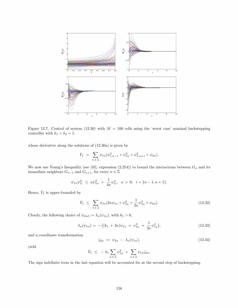
0 0.1 0.2 0.3 0.4 0.5 0.6 0.7 0.8−1
0
1
2
3
4
5
6
t
Ψ1(t)
0 2 4 6 8 10−1
−0.5
0
0.5
1
t
Ψ1(t)
0 2 4 6 8 10−1.5
−1
−0.5
0
0.5
1
t
Ψ2(t)
0 2 4 6 8 10
−4
−3
−2
−1
0
1
2
t
U(t)
Figure 12.7: Control of system (12.30) with M = 100 cells using the ‘worst case’ nominal backsteppingcontroller with k1 = k2 = 1.
whose derivative along the solutions of (12.30a) is given by
V1 =∑n∈Z
ψ1n(ψ21,n−1 + ψ2
1n + ψ21,n+1 + ψ2n).
We now use Young’s Inequality (see [45], expression (2.254)) to bound the interactions between Gn and itsimmediate neighbors Gn−1 and Gn+1, for every n ∈ Z
ψ1nψ21i ≤ κψ2
1n +14κψ4
1i, κ > 0, i = n− 1, n+ 1.
Hence, V1 is upper-bounded by
V1 ≤∑n∈Z
ψ1n(2κψ1n + ψ21n +
12κψ3
1n + ψ2n). (12.32)
Clearly, the following choice of ψ2nd := λn(ψ1n), with k1 > 0,
λn(ψ1n) = −((k1 + 2κ)ψ1n + ψ2
1n +12κψ3
1n
), (12.33)
and a coordinate transformationζ2n := ψ2n − λn(ψ1n), (12.34)
yieldV1 ≤ − k1
∑n∈Z
ψ21n +
∑n∈Z
ψ1nζ2n.
The sign indefinite term in the last equation will be accounted for at the second step of backstepping.
158

Step 2 CLF from Step 1 is augmented by a term which penalizes the deviation of ψ2n from ψ2nd
V2(Ψ1,Z2) := V1(Ψ1) +12
∑n∈Z
ζ22n.
The derivative of V2 along the solutions of
ψ1n = − k1ψ1n + ζ2n, n ∈ Z,
ζ2n = − ∂λn(ψ1n)∂ψ1n
(f1n(Ψ1) + ψ2n) + un, n ∈ Z,
is determined by
V2 ≤ − k1
∑n∈Z
ψ21n +
∑n∈Z
ζ2n(ψ1n − ∂λn(ψ1n)∂ψ1n
(f1n(Ψ1) + ψ2n) + un).
We choose a control law of the form
un = − (ψ1n − ∂λn(ψ1n)∂ψ1n
(f1n(Ψ1) + ψ2n) + k2ζ2n), (12.35)
with k2 > 0, to obtainV2 ≤ − k1
∑n∈Z
ψ21n − k2
∑n∈Z
ζ22n.
Hence, controller (12.35) guarantees global exponential stability of the origin of the infinite dimensionalsystem (12.30). This controller has the very same architecture as the original plant: the n-th controller cellKn interacts only with its nearest neighbors Kn−1 and Kn+1.
Figure 12.8 shows simulation results of uncontrolled (upper left) and controlled system (12.30) with M =100 cells using the nearest neighbor interaction backstepping controller (12.33,12.34,12.35) with k1 = k2 = 1and κ = 0.5. The initial state of the system is randomly selected. The desired control objective is achievedwith a good quality of the transient response and a reasonable amount of control effort.
Fully decentralized controller
Step 1 We start the recursive design with subsystem (12.30a) by proposing a CLF (12.31). The derivativeof V1(Ψ1) along the solutions of (12.30a) is determined by (12.32). However, we now choose a ‘stabilizingfunction’ ψ2nd := λn(ψ1n) of the form
λn(ψ1n) = −((k1 + 2κ)ψ1n + ψ2
1n + (k0 +12κ
)ψ31n
), (12.36)
with k0, k1 > 0, which clearly renders V1 negative definite. Coordinate transformation ζ2n := ψ2n− λn(ψ1n)yields
V1 ≤ − k1
∑n∈Z
ψ21n − k0
∑n∈Z
ψ41n +
∑n∈Z
ψ1nζ2n.
The sign indefinite term in the last equation will be taken care of at the second step of backstepping.Step 2 The second step of our design closely follows the procedure outlined in the nearest neighbor controllerdesign. The only difference is that we employ the Young’s inequality to upper-bound
ζ2n∂λn(ψ1n)∂ψ1n
ψ21i ≤ κ
(ζ2n
∂λn(ψ1n)∂ψ1n
)2
+14κψ4
1i, κ > 0, ∀n ∈ Z, ∀ i = n− 1, n+ 1,
in the expression for the temporal derivative of V2(Ψ1,Z2) := V1(Ψ1)+ 12
∑n∈Z
ζ22n. This allows us to choose
159

0 0.1 0.2 0.3 0.4 0.5 0.6 0.7 0.8−1
0
1
2
3
4
5
6
t
Ψ1(t)
0 2 4 6 8 10−1
−0.5
0
0.5
1
t
Ψ1(t)
0 2 4 6 8 10−1.5
−1
−0.5
0
0.5
1
t
Ψ2(t)
0 2 4 6 8 10−8
−6
−4
−2
0
2
t
U(t)
Figure 12.8: Control of system (12.30) withM = 100 cells using the nearest neighbor interaction backsteppingcontroller (12.33,12.34,12.35) with k1 = k2 = 1 and κ = 0.5.
a fully decentralized controller of the form
un = −(ψ1n − ∂λn(ψ1n)
∂ψ1n(ψ2
1n + ψ2n) + (ψ2n − λn(ψ1n))(k2 + 2κ(∂λn(ψ1n)∂ψ1n
)2)), (12.37)
with k2 > 0, to obtain
V2 ≤ − k1
∑n∈Z
ψ21n − (k0 − 1
2κ)∑n∈Z
ψ41n − k2
∑n∈Z
ζ22n.
Thus, controller (12.37) with κ > 0, k0 ≥ 12κ , k1 > 0, and k2 > 0 guarantees global asymptotic stability of
the origin of the infinite dimensional system (12.30). This controller is fully decentralized: the n-th controllercell Kn interacts only with the plant cell on which it acts Gn.
Figure 12.9 shows simulation results of uncontrolled (upper left) and controlled system (12.30) withM = 100 cells using the fully decentralized backstepping controller (12.36,12.37) with k0 = k1 = k2 = 1and κ = 0.5. The initial state of the system is randomly selected. Clearly, the fully decentralized controllerrequires big amount of initial effort to account for the lack of information about interactions between differentsubsystems. We note that there is some room for improvement of these large initial excursions of controlsignals by the different choice of design parameters k0, k1, k2, and κ. However, the obtained results seem tobe in agreement with our intuition:
• Higher gain is required to achieve the desired control objective when controller cells donot communicate with each other.
Remark 5 Neither a distributed controller with the nearest neighbor interactions nor a fully decentralizedcontroller for system (12.30) can be obtained using the individual cell backstepping procedure of § 12.3.2.This is because the harmful interactions–that are dominated by feedback in the global design–are treated asthe exogenous signals in the individual cell design. Thus, the ‘worst case’ backstepping controller in whichKn interacts with Kn−2,Kn−1,Kn+1,Kn+2 is pretty much the only controller that can come out of theindividual cell backstepping design.
160

0 0.1 0.2 0.3 0.4 0.5 0.6 0.7 0.8−1
0
1
2
3
4
5
6
t
Ψ1(t)
0 2 4 6 8 10−1
−0.5
0
0.5
1
t
Ψ1(t)
0 2 4 6 8 10−3.5
−3
−2.5
−2
−1.5
−1
−0.5
0
0.5
1
1.5
t
Ψ2(t)
0 2 4 6 8 10
−300
−250
−200
−150
−100
−50
0
50
t
U(t)
Figure 12.9: Control of system (12.30) with M = 100 cells using the fully decentralized backsteppingcontroller (12.36,12.37) with k0 = k1 = k2 = 1 and κ = 0.5.
12.5 Adaptive state-feedback distributed backstepping design
In this section, we consider adaptive state-feedback distributed design. We study systems with both spatiallyconstant and spatially varying unknown parameters. We assume that these parametric uncertainties do notdepend on time. The dynamic controllers that guarantee boundedness of all signals in the closed-loop andachieve ‘regulation’ of the plant’s state are obtained using backstepping approach.
We show that systems with constant unknown parameters are amenable to a global design. In otherwords, an Adaptive CLF (ACLF) can be constructed for the entire infinite dimensional system. Based on ourexperience with nominal backstepping this may seem advantageous, but we demonstrate that this approachyields centralized dynamical controllers, which is clearly undesirable. On the other hand, for systems withspatially varying unknown parameters global design is not possible without some a priori information aboutvalues of these parameters. For this class of systems we perform an individual cell adaptive backsteppingdesign which results into distributed localized dynamical controllers. As in the nominal case, the architectureof these controllers has strong similarity with the plant architecture. Furthermore, the dynamical order ofKn depends on the number of unknown parameters in Gn, and it increases as the number of integratorsbetween unknown parameters and the location at which control enters increases. We also note that thisapproach can be utilized to obtain decentralized adaptive controllers for systems with constant unknownparameters.
Remark 6 The adaptive control design problems are solved for systems whose local dynamical order is equalto 2. For systems with m > 2 the appropriately modified tuning functions design [45] can be employed toguarantee desired dynamical properties.
12.5.1 Constant unknown parameters
We first study adaptive state-feedback design for systems with constant unknown parameters (12.7). Weestablish that global adaptive backstepping design yields centralized distributed controllers.
161

For m = 2, (12.7) simplifies to
ψ1n = ν1n(Ψ1) + g∗1n(Ψ1)θ1 + ψ2n, n ∈ Z, (12.38a)
ψ2n = ν2n(Ψ1,Ψ2) + g∗2n(Ψ1,Ψ2)θ2 + bun, n ∈ Z, (12.38b)
where θ1 ∈ Rr1 , θ2 ∈ R
r2 , and b ∈ R represent constant unknown parameters. We rewrite dynamics of theentire system as
Ψ1 = N1(Ψ1) + G∗1 (Ψ1)θ1 + Ψ2, (12.39a)
Ψ2 = N2(Ψ1,Ψ2) + G∗2 (Ψ1,Ψ2)θ2 + bU, (12.39b)
where G1 and G2 are operators (Gk : l2 → Rrk , k = 1, 2) defined by
G1(Ψ1) :=[· · · g1,n−1(Ψ1) g1n(Ψ1) g1,n+1(Ψ1) · · ·
],
G2(Ψ1,Ψ2) :=[· · · g2,n−1(Ψ1,Ψ2) g2n(Ψ1,Ψ2) g2,n+1(Ψ1,Ψ2) · · ·
].
Clearly, the adjoints of these two operators are respectively given by
G∗1 (Ψ1) :=
...g∗1,n−1(Ψ1)
g∗1n(Ψ1)
g∗1,n+1(Ψ1)...
, G∗
2 (Ψ1,Ψ2) :=
...g∗2,n−1(Ψ1,Ψ2)
g∗2n(Ψ1,Ψ2)
g∗2,n+1(Ψ1,Ψ2)...
.
Using Assumptions 1 and 3, we conclude boundedness of these two operators.In the adaptive backstepping design we have to account for the lack of knowledge of parameters in (12.39).
In other words, we need to estimate the values of unknown parameters θ1, θ2, and reciprocal of unknowncontrol coefficient b, := 1/b, to avoid the division with an estimate of b which can occasionally assume zerovalue.Step 1 We invoke Assumption 6, and start the global recursive design with subsystem (12.39a) by consideringΨ2 as control and proposing a radially unbounded ACLF Va1 : l2 × R
r1 → R of the form
Va1(Ψ1, θ1) =12〈Ψ1,Ψ1〉 +
12θ∗1Γ−1
1 θ1, (12.40)
where θ1(t) := θ1 − θ1(t), and Γ1 ∈ Rr1×r1 is a positive definite matrix (Γ1 = Γ∗
1 > 0). ACLF (12.40) isobtained by augmenting the nominal CLF of § 12.3.1 by a term that accounts for the error between unknownparameter θ1 and its estimate θ1.
The derivative of Va1(Ψ1, θ1) along the solutions of (12.39a) is given by
Va1 =⟨Ψ1,N1(Ψ1) + G∗
1 (Ψ1)θ1 + Ψ2
⟩+ θ∗1
(Γ−1
1˙θ1 + G1(Ψ1)Ψ1
).
With the following choice of ‘stabilizing function’ Ψ2d
Ψ2d := Λ(Ψ1, θ1) = −(N1(Ψ1) + G∗
1 (Ψ1)θ1 + k1Ψ1
), k1 > 0,
and a change of coordinatesZ2 := Ψ2 − Λ(Ψ1, θ1),
we obtainVa1 = − k1 〈Ψ1,Ψ1〉 + 〈Z2,Ψ1〉 + θ∗1
(Γ−1
1˙θ1 + G1(Ψ1)Ψ1
).
162

The last two terms on the right-hand side of (12.41) will be taken care of at the second step of backstepping.Step 2 We start the second step of our design by augmenting ACLF (12.40) by three terms that account forthe errors between Ψ2 and Ψ2d, and the errors between unknown parameters θ2 and and their estimatesθ2 and
Va2(Ψ1,Z2, θ1, θ2, ) := Va1(Ψ1, θ1) +12〈Z2,Z2〉 +
12θ∗2Γ−1
2 θ2 +|b|2β2, (12.41)
where θ2(t) := θ2 − θ2(t), (t) := − (t), Γ2 ∈ Rr2×r2 is a positive definite matrix, and β is a positive
constant. The derivative of Va2 along the solutions of
Ψ1 = − k1Ψ1 + Z2 + G∗1 θ1,
Z2 = N2 + G∗2 (θ2 + θ2) − ∂Λ(Ψ1, θ1)
∂Ψ1
(N1 + G∗
1 (θ1 + θ1) + Ψ2
)− ∂Λ(Ψ1, θ1)
∂θ1
˙θ1 + bU,
is determined by
Va2 = − k1 〈Ψ1,Ψ1〉 + 〈Z2,S + bU〉 + θ∗2(Γ−1
2˙θ2 + G2Z2
)+
|b|β ˙
+ θ∗1
(Γ−1
1˙θ1 + G1Ψ1 − G1
(∂Λ(Ψ1, θ1)
∂Ψ1
)∗Z2
) (12.42)
where
S := Ψ1 + N2 + G∗2 θ2 − ∂Λ(Ψ1, θ1)
∂Ψ1
(N1 + G∗
1 θ1 + Ψ2
)− ∂Λ(Ψ1, θ1)
∂θ1
˙θ1
We can eliminate θ1 and θ2 from (12.42) with the following parameter update laws
˙θ1 = Γ1G1(Ψ1)
(Ψ1 −
(∂Λ(Ψ1, θ1)
∂Ψ1
)∗ (Ψ2 − Λ(Ψ1, θ1)
)),
˙θ2 = Γ2G2(Ψ1,Ψ2)
(Ψ2 − Λ(Ψ1, θ1)
).
(12.43)
A choice of control law of the form
U = − (S + k2Z2) , k2 > 0,
together with (12.43) and the relationship
b = b(− ) = 1 − b,
renders (12.42) into
Va2 = − k1 〈Ψ1,Ψ1〉 − k2 〈Z2,Z2〉 +|b|β( ˙ + β sign(b) 〈Z2,S + k2Z2〉
). (12.44)
With the following choice of update law for the estimate
˙ = β sign(b) 〈Z2,S + k2Z2〉 ,
(12.44) simplifies to
Va2 = − k1 〈Ψ1,Ψ1〉 − k2 〈Z2,Z2〉 =: −W (Ψ1,Z2) ≤ 0. (12.45)
We next establish boundedness of all signals in the closed-loop and asymptotic convergence of Ψ1 andΨ2 to zero.
163

Establishing asymptotic convergence of Ψ1 and Ψ2 to zero
Negative semi-definiteness of Va2 implies that Va2 is a non-increasing function of time. We note that prop-erties of functions ν1n and g1n (see Assumptions 1–3) together with Assumption 6 guarantee boundednessof Va2 at t = 0. Hence, based on the definition of Va2 and its boundedness at t = 0, we conclude that Ψ1,Ψ2, θ1, θ2, and are globally uniformly bounded, that is,
‖Ψk(t)‖2 :=∑n∈Z
ψ2kn(t) < ∞
‖θk(t)‖2 := θ∗k(t)θk(t) < ∞
‖(t)‖2 := 2(t) < ∞
∀ t ≥ 0, k = 1, 2.
In view of the last equation, properties of functions gkn and νkn (see Assumptions 1–3), and definition of U,it follows that
θ1 ∈ L∞, θ2 ∈ L∞, ∈ L∞, ψ1n ∈ L∞, ψ2n ∈ L∞, un ∈ L∞, ∀n ∈ Z ,
which in turn impliesψ1n ∈ L∞, ψ2n ∈ L∞, ∀n ∈ Z.
Using Assumption 3 and the fact that Ψ1(t) ∈ l2, Ψ2(t) ∈ l2, ∀ t ≥ 0, we also conclude that ˙θ1(t) < ∞,
˙θ2(t) <∞, ˙(t) <∞, ∀ t ≥ 0. This follows from the properties of functions νkn and gkn (see Assumptions 1–3) and a simple observation that Ψ(t) ∈ lp × lq, ∀ t ≥ 0, ∀ p, q ∈ (2, ∞) whenever Ψ(t) ∈ l2 × l2, ∀ t ≥ 0.Furthermore, since Va2(Ψ1(t),Z2(t), θ1(t), θ2(t), (t)) is a non-increasing non-negative function, it has a limitVa2∞ as t→ ∞. Therefore, integration of (12.45) yields∫ ∞
0
W (Ψ1(t),Z2(t)) dt = k1
∫ ∞
0
〈Ψ1(t),Ψ1(t)〉 dt + k2
∫ ∞
0
〈Z2(t),Z2(t)〉 dt
≤ Va2(Ψ1(0),Z2(0), θ1(0), θ2(0), (0)) − Va1∞
< ∞,
which together with the definition of Z2 implies
ψ1n ∈ L2, ψ2n ∈ L2, ∀n ∈ Z.
Therefore, we have shown that
ψ1n, ψ2n ∈ L2 ∩ L∞, ψ1n, ψ2n ∈ L∞, ∀n ∈ Z.
Using the Barbalat lemma (see, for example [44, 57, 66]), we conclude that both ψ1n(t) and ψ2n(t) go tozero as t → ∞, for all n ∈ Z. Therefore, the dynamical controller obtained as a result of our designguarantees boundedness of all signals in the closed-loop and asymptotic convergence of the state Ψ∗(t) :=[
Ψ∗1(t) Ψ∗
2(t)]∗ of (12.39) to zero.
The developments of this subsection are summarized in the following theorem.
Theorem 21 Suppose that system (12.39) satisfies Assumptions 1, 2, 3, 4, and 6. Then, the following
164

centralized dynamical controller
U = − (S + k2Z2) , k2 > 0,
Z2 = Ψ2 − Λ(Ψ1, θ1),
S = Ψ1 + N2 + G∗2 θ2 − ∂Λ(Ψ1, θ1)
∂Ψ1
(N1 + G∗
1 θ1 + Ψ2
)− ∂Λ(Ψ1, θ1)
∂θ1
˙θ1,
Λ = − (N1(Ψ1) + G∗1 (Ψ1)θ1 + k1Ψ1), k1 > 0,
˙θ1 = Γ1G1(Ψ1)
(Ψ1 −
(∂Λ(Ψ1, θ1)
∂Ψ1
)∗Z2
),
˙θ2 = Γ2G2(Ψ1,Ψ2)Z2,
˙ = β sign(b) 〈Z2,S + k2Z2〉 ,
(12.46)
guarantees boundedness of all signals in the closed-loop system (12.39,12.46) and asymptotic convergence ofthe state of (12.39) to zero. These properties can be established with the Lyapunov function
Va2(Ψ1,Z2, θ1, θ2, ) :=12〈Ψ1,Ψ1〉 +
12〈Z2,Z2〉 +
12θ∗1Γ−1
1 θ1 +12θ∗2Γ−1
2 θ2 +|b|2β2.
Remark 7 Since information from all plant cells is used to determine estimates of constant unknown pa-rameters θ1 ∈ R
r1 , θ2 ∈ Rr2 , and ∈ R, dynamical controller (12.46) in Theorem 21 is centralized. This
controller builds one estimate per unknown parameter, and its dynamical order is equal to r1 + r2 + 1.
12.5.2 Spatially varying unknown parameters
Here we consider state-feedback design for systems with time independent spatially varying unknown pa-rameters. An example of such a system is given by (12.8), which for m = 2 becomes
ψ1n = τ1n(Ψ1) + h∗1n(Ψ1)θ1n + ψ2n, n ∈ Z, (12.47a)
ψ2n = τ2n(Ψ1,Ψ2) + h∗2n(Ψ1,Ψ2)θ2n + bnun, n ∈ Z. (12.47b)
Remark 8 Even if Assumption 6 holds, the infinite number of unknown parameters in (12.47) prevents usfrom doing a global design. Namely, the finiteness of the global ACLF candidate for (12.47a) at t = 0
Va1(Ψ1, θ1nn∈Z) :=12〈Ψ1,Ψ1〉 +
12
∑n∈Z
θ∗1nΓ−11n θ1n,
would imply that most of unknown parameters are initially known, which is somewhat artificial. If we havesome a priori information about values that the unknown parameters can assume we can choose a sequenceof positive definite matrices Γ1nn∈Z
such that Va1(Ψ1(0), θ1n(0)n∈Z) is finite. However, this would leadto parameter update laws with very large gains since elements of this sequence have to increase their valuesas n→ ∞. Clearly, this is not desirable for implementation.
In view of Remark 8, we carry out the individual cell adaptive backstepping design for system (12.47)with spatially varying parametric uncertainties. This approach can be also used for adaptive control ofsystems with constant unknown parameters, and we will demonstrate that it yields distributed dynamicalcontrollers that are not centralized. Thus, individual cell adaptive design for infinite dimensional systemson lattices has advantages over global adaptive design of § 12.5.1, because the latter leads to centralizeddynamical controllers.Step 1 For the n-th cell of subsystem (12.47a) we propose an ACLF
Va1n(ψ1n, θ1n) =12ψ2
1n +12θ∗1nΓ
−11n θ1n,
165
and choose a desired value of ‘virtual control’
ψ2nd := λn(Ψ1, θ1n) = − (τ1n(Ψ1) + h∗1n(Ψ1)θ1n + k1nψ1n), k1n > 0,
to obtainVa1n = − k1nψ
21n + ψ1nζ2n + θ∗1n
(Γ−1
1n˙θ1n + ψ1nh1n(Ψ1)
),
where ζ2n := ψ2n − λn(Ψ1, θ1n). The sign indefinite terms in Va1n will be accounted for at the second stepof adaptive design.Step 2 The derivative of ζ2n is now determined by
ζ2n = τ2n(Ψ1,Ψ2) + h∗2n(Ψ1,Ψ2)(θ2n + θ2n) + bnun − ∂λn(Ψ1, θ1n)∂Ψ1
Ψ1 − ∂λn(Ψ1, θ1n)
∂θ1n
˙θ1n.
Using Assumption 1 and the definition of λn(Ψ1, θ1n) we express (∂λn/∂Ψ1)Ψ1 as
∂λn∂Ψ1
Ψ1 =∑j∈ZN
∂λn∂ψ1,n+j
ψ1,n+j =∑j∈ZN
θ∗1,n+jh1,n+j(Ψ1)∂λn
∂ψ1,n+j+
∑j∈ZN
∂λn∂ψ1,n+j
(τ1,n+j(Ψ1) + h∗1,n+j(Ψ1)θ1,n+j + ψ2,n+j
).
Since θ1,n+jj∈ZNenters into the expression for ζ2n, we augment the ACLF from Step 1 as follows
Va2n(ψ1n, ζ2n, θ1,n+jj∈ZN, θ2n, n) :=
Va1n(ψ1n, θ1n) +12ζ22n +
12
∑j∈ZN\0
θ∗1,n+jΓ−11,n+j θ1,n+j +
12θ∗2nΓ
−12n θ2n +
12|bn|βn
2n,
It is readily established that a distributed dynamical controller of the form
un = − n(sn + k2nζ2n),
˙θ1n =
(ψ1n − ζ2n
∂λn∂ψ1n
)Γ1nh1n(Ψ1),
˙θ1,n+j = − ζ2n
∂λn∂ψ1,n+j
Γ1,n+jh1,n+j(Ψ1), j ∈ ZN \ 0,
˙θ2n = ζ2nΓ2nh2n(Ψ1,Ψ2),˙n = βn sign(bn)ζ2n (sn + k2nζ2n) ,
sn = ψ1n + τ2n + h∗2nθ2n − ∂λn
∂θ1n
˙θ1n −∑
j∈ZN
∂λn∂ψ1,n+j
(τ1,n+j + h∗1,n+j θ1,n+j + ψ2,n+j
),
renders Va2n intoVa2n = − k1nψ
21n − k2nζ
22n =: −Wn(ψ1n, ζ2n) ≤ 0,
where we use the analytical expression for ˙θ1n in the expression for sn.
Using similar argument as in § 12.5.1, we establish boundedness of all signals in the closed-loop andasymptotic convergence of both ψ1n(t) and ψ2n(t) to zero, for all n ∈ Z.
The main result of this subsection is summarized in the following theorem.
Theorem 22 Suppose that system (12.47) satisfies Assumptions 1, 2, and 5. Then, the following distributed
166
dynamical controller
un = − n(sn + k2nζ2n), k2n > 0, ∀n ∈ Z,
ζ2n = ψ2n − λn(Ψ1, θ1n),
λn = − (τ1n(Ψ1) + h∗1n(Ψ1)θ1n + k1nψ1n), k1n > 0, ∀n ∈ Z,
sn = ψ1n + τ2n + h∗2nθ2n − ∂λn
∂θ1n
˙θ1n −∑
j∈ZN
∂λn∂ψ1,n+j
(τ1,n+j + h∗1,n+j θ1,n+j + ψ2,n+j
),
˙θ1n =
(ψ1n − ζ2n
∂λn∂ψ1n
)Γ1nh1n(Ψ1),
˙θ1,n+j = − ζ2n
∂λn∂ψ1,n+j
Γ1,n+jh1,n+j(Ψ1), j ∈ ZN \ 0,
˙θ2n = ζ2nΓ2nh2n(Ψ1,Ψ2),˙n = βn sign(bn)ζ2n (sn + k2nζ2n) ,
(12.48)
guarantees boundedness of all signals in the closed-loop system (12.47,12.48) and asymptotic convergence ofthe state of (12.47) to zero.
Theorem 22 can be used to derive the following corollary for localized adaptive distributed control ofsystems with constant parametric uncertainties.
Corollary 23 Suppose that system (12.38) satisfies Assumptions 1, 2, and 4. Then, the following distributeddynamical controller
un = − n(sn + k2nζ2n), k2n > 0, ∀n ∈ Z,
ζ2n = ψ2n − λn(Ψ1, θ1n),
λn = − (ν1n(Ψ1) + g∗1n(Ψ1)θ1n + k1nψ1n), k1n > 0, ∀n ∈ Z,
sn = ψ1n + ν2n + g∗2nθ2n − ∂λn
∂θ1n
˙θ1n −∑
j∈ZN
∂λn∂ψ1,n+j
(ν1,n+j + g∗1,n+j θ1n + ψ2,n+j
),
˙θ1n = Γ1n
ψ1ng1n(Ψ1) − ζ2n
∑j∈ZN
∂λn∂ψ1,n+j
g1,n+j(Ψ1)
,
˙θ2n = ζ2nΓ2ng2n(Ψ1,Ψ2),˙n = βn sign(bn)ζ2n (sn + k2nζ2n) ,
(12.49)
guarantees boundedness of all signals in the closed-loop system (12.38,12.49) and asymptotic convergence ofthe state of (12.38) to zero.
12.6 Dynamical order induced by adaptive distributed backstep-ping design
As noted in Remark 7, since information from all plant cells is used to determine estimates of constantunknown parameters, the adaptive backstepping design of § 12.5.1 yields centralized dynamical controllers.On the other hand, the adaptive backstepping design of § 12.5.2 results into localized distributed dynamicalcontrollers. The architecture of these controllers enjoys the same properties as in the nominal case:
167

• When matching condition is satisfied, the adaptive distributed backstepping controllersof § 12.5.2 inherit the plant architecture.
• For systems (12.38) and (12.47) with 2N interactions per plant cell, the adaptive dis-tributed backstepping design § 12.5.2 induces 4N interactions per controller cell.
There are two important differences between nominal and adaptive backstepping designs:
• Nominal controllers are static, whereas adaptive controllers are dynamic.
• As illustrated in § 12.4, nominal controllers with less interactions can be obtained by performing aglobal design to identify beneficial interactions, and/or to dominate harmful interactions. On theother hand, even though the individual cell adaptive backstepping design yields localized distributedcontrollers, it does not seem that it lends itself easily to design of controllers with less interactions.
We next comment on the dynamical order induced by adaptive distributed backstepping design.
Constant unknown parameters
The design of § 12.5.1 yields centralized finite dimensional controller (12.46) in which both the dynamicalorder and the number of parameter estimates are equal to the number of unknown parameters. In otherwords, for system (12.39) with constant unknown parameters θ1 ∈ R
r1 , θ2 ∈ Rr2 , and ∈ R, controller (12.46)
has an estimate per unknown parameter (i.e., θ1, θ2, and ), and its dynamical order is equal to r1 + r2 + 1.On the other hand, controller (12.49) has different parameter update laws (for θ1n, θ2n, and n) in everycontrol unit Kn, even though all unknown parameters are both spatially and temporally constant. Thedynamical order of Kn, for every n ∈ Z, is equal to the number of unknown parameters: r1 + r2 + 1.This ‘over-parameterization’ is advantageous in applications because it allows for implementation of localizedadaptive distributed controllers. This useful property cannot be achieved with controller (12.46) becauseit requires information about entire distributed state to estimate unknown parameters. Furthermore, thedesign procedure described in § 12.5.2 (see Corollary 23) does not require Assumptions 3 and 6 to hold and,consequently, it can be applied to a broader class of problems.
Spatially varying unknown parameters
The individual cell adaptive backstepping design of § 12.5.1 yields localized adaptive distributed controllers.For systems with spatially varying unknown parameters, the dynamical order of these controllers is deter-mined by two factors: the number of interactions per plant cell, and the number of unknown parameters. If,for simplicity, we assume that, for every n ∈ Z, θ1n ∈ R
r1 , θ2n ∈ Rr2 , and n ∈ R then the local dynamical
order of controller (12.48) in Theorem 22 is equal to (2N + 1)r1 + r2 + 1. Thus, for system (12.47) that doesnot satisfy the matching condition, the dynamical order of Kn scales linearly with the number of interactionsper plant cell. Clearly, this order can become prohibitive for systems with large number of interactions perplant cell.
12.7 Output-feedback distributed backstepping design
The controllers of § 12.3 and § 12.5 provide stability/regulation/asymptotic tracking of the closed-loopsystems under the assumption that the full state information is available. In this section, we study a morerealistic situation in which only a distributed output is measured. We show that, as for finite dimensionalsystems [45], the observer backstepping can be used as a tool for fulfilling the desired control objective forsystems on lattices in which nonlinearities depend only on the measured signals. The starting point of thenominal output-feedback approach is a design of an observer which guarantees the exponential convergenceof the state estimates to their real values. Once this is accomplished, the combination of backstepping andnonlinear damping is used to account for the observation errors and provide closed-loop stability. In theadaptive case, filters which provide ‘virtual estimates’ of unmeasured state variables also need to be designed.
168

We solve output-feedback problems for systems of local dynamical order two (m = 2) that satisfy thematching condition. General case can be handled using similar tools. In this situation, systems (12.9)and (12.10) respectively simplify to
ψ1n = ψ2n, n ∈ Z, (12.50a)
ψ2n = fn(Y) + bnun, n ∈ Z, (12.50b)yn = ψ1n, n ∈ Z, (12.50c)
and systems with parametric uncertainties
ψ1n = ψ2n, n ∈ Z, (12.51a)
ψ2n = τn(Y) + h∗n(Y)θn + bnun, n ∈ Z, (12.51b)yn = ψ1n, n ∈ Z. (12.51c)
Both nominal and adaptive output-feedback problems are solved using individual cell backstepping design.We note that nominal output-feedback problem can be also solved using global backstepping design if theinitial state of system (12.50) satisfies Assumption 6.
12.7.1 Nominal output-feedback design
We rewrite (12.50) in a form suitable for observer design
ψn = Aψn + ϕn(Y) + bne2un, n ∈ Z, (12.52a)yn = Cψn, n ∈ Z, (12.52b)
where
ψn :=[ψ1n
ψ2n
], ϕn(Y) :=
[0
fn(Y)
], A :=
[0 10 0
], e2 :=
[01
], C :=
[1 0
].
We proceed by designing an equivalent of Krener-Isidori observer (see, for example, [45, 67]) for (12.52)
˙ψn = Aψn + Ln(yn − yn) + ϕn(Y) + bne2un, n ∈ Z, (12.53a)
yn = Cψn, n ∈ Z, (12.53b)
where Ln :=[l1n l2n
]∗ is chosen such that A0n := A−LnC is a Hurwitz matrix for every n ∈ Z. Clearly,this is going to be satisfied if and only if lin > 0, ∀ i = 1, 2, ∀n ∈ Z. In this case, an exponentially stablesystem of the form
˙ψn = A0nψn, n ∈ Z, (12.54)
is obtained by subtracting (12.53) from (12.52). The properties of A0n imply the exponential convergenceof ψn := ψn − ψn to zero and the existence of the positive definite matrix P0n that satisfies
A∗0nP0n + P0nA0n = − I, ∀n ∈ Z. (12.55)
We are now ready to design an output-feedback controller that guarantees stability of (12.50).Step 1 The observer-backstepping design starts with subsystem (12.50a) by rewriting it as
ψ1n = ψ2n + ψ2n, n ∈ Z, (12.56)
and considering ψ2n as a virtual control and ψ2n as a disturbance generated by (12.54). We propose a CLF
169

for the n-th subsystem of (12.56)
V1n(ψ1n, ψn) :=12ψ2
1n +1d1n
ψ∗nP0nψn,
where P0n is a positive definite matrix that satisfies (12.55), and d1n > 0 is a design parameter. Thederivative of V1n along the solutions of (12.56,12.54) for every n ∈ Z is determined by
V1n = ψ1n(ψ2n + ψ2n) − 1d1n
‖ψn‖22
≤ ψ1n(ψ2n + d1nψ1n) +1
4d1nψ2
2n − 1d1n
‖ψn‖22
≤ ψ1n(ψ2n + d1nψ1n) − 34d1n
‖ψn‖22,
(12.57)
where Young’s Inequality (see [45], expression (2.254)) is used to upper bound ψ1nψ2n. The following choiceof a ‘stabilizing function’ ψ2nd
ψ2nd = − (k1n + d1n)ψ1n, k1n > 0, ∀n ∈ Z,
clearly renders V1n(ψ1n, ψn) negative definite. Since ψ2n is not actually a control, but rather, an estimate ofa state variable, we introduce the change of variables
ζ2n := ψ2n − ψ2nd = ψ2n + (k1n + d1n)ψ1n, ∀n ∈ Z,
which adds an additional term on the right-hand side of (12.57)
V1n ≤ − k1nψ21n − 3
4d1n‖ψn‖2
2 + ψ1nζ2n. (12.58)
The sign indefinite term in (12.58) will be taken care of at the second step of backstepping.Step 2 We express our system into new coordinates as
ψ1n = − (k1n + d1n)ψ1n + ζ2n + ψ2n, n ∈ Z, (12.59a)
ζ2n = (k1n + d1n)(ψ2n + ψ2n) + l2n(ψ1n − ψ1n) + fn(Y) + bnun, n ∈ Z, (12.59b)
˙ψn = A0nψn, n ∈ Z, (12.59c)
and propose the following CLF for its n-th subsystem
V2n(ψ1n, ζ2n, ψn) := V1n(ψ1n, ψn) +12ζ22n +
1d2n
ψ∗nP0nψn,
with d2n > 0. The derivative of V2n along the solutions of (12.59) for every n ∈ Z is determined by
V2n = V1n + ζ2nζ2n − 1d2n
‖ψn‖22 ≤ − k1nψ
21n − 3
4(
1d1n
+1d2n
)‖ψn‖22 +
ζ2n(ψ1n + (k1n + d1n)ψ2n + l2n(ψ1n − ψ1n) + fn(Y) + d2n(k1n + d1n)2ζ2n + bnun).
A control law of the form
un = − 1bn
(ψ1n + (k1n + d1n)ψ2n + l2n(ψ1n − ψ1n) + fn(Y) + d2n(k1n + d1n)2ζ2n + k2nζ2n), (12.60)
170

with k2n > 0 for every n ∈ Z, guarantees negative definiteness of V2n, that is
V2n ≤ − k1nψ21n − k2nζ
22n − 3
4(
1d1n
+1d2n
)‖ψn‖22.
Hence, we conclude global asymptotic stability of the origin of closed-loop system (12.50,12.54,12.60).
12.7.2 Adaptive output-feedback design
We rewrite (12.51) in a form suitable for adaptive output-feedback design
ψn = Aψn + ηn(Y) +r∑j=1
θjnϕjn(Y) + bne2un, n ∈ Z, (12.61a)
yn = Cψn, n ∈ Z, (12.61b)
where
ψn :=[ψ1n
ψ2n
], ηn(Y) :=
[0
τn(Y)
], ϕjn(Y) :=
[0
hjn(Y)
],
A :=[
0 10 0
], e2 :=
[01
], C :=
[1 0
].
We proceed by designing filters which provide ‘virtual estimates’ of unmeasured state variables (see [45],§ 7.3)
ξ(0)n = A0nξ(0)n + Lnyn + ηn(Y), n ∈ Z, (12.62a)
ξ(j)n = A0nξ(j)n + ϕjn(Y), 1 ≤ j ≤ r, n ∈ Z, (12.62b)
vn = A0nvn + e2un, n ∈ Z, (12.62c)
where Ln :=[l1n l2n
]∗ is chosen such that A0n := A− LnC is Hurwitz for every n ∈ Z. Clearly, A0n isgoing to be Hurwitz if and only if lin > 0, ∀ i = 1, 2, ∀n ∈ Z. In this case, an exponentially stable systemof the form
εn = A0nεn, εn := ψn − ξ(0)n +r∑j=1
θjnξ(j)n + bnvn, n ∈ Z, (12.63)
is obtained by combining (12.61) and (12.62). The properties of A0n imply the exponential convergence ofεn to zero and the existence of the positive definite matrix P0n that satisfies (12.55).
We are now ready to design an adaptive output-feedback controller for (12.51) using backstepping.Step 1 The adaptive observer-backstepping design starts with subsystem (12.51a) by rewriting it as
ψ1n = ξ(0)2n +
r∑j=1
θjnξ(j)2n + bnv2n + ε2n, n ∈ Z, (12.64)
and considering v2n as a virtual control and ε2n as a disturbance generated by (12.63). If v2n were control,and all parameters were known, then (12.64) could be stabilized by
v2n = − 1bn
ξ(0)2n + (k1n + d1n)ψ1n
−
r∑j=1
θjnbnξ(j)2n , n ∈ Z, (12.65)
where k1n and d1n are positive design parameters. To account for parametric uncertainties we add and
171

subtract the right-hand side of (12.65) to v2n in (12.64) to obtain
ψ1n = − (k1n + d1n)ψ1n + bn
v2n + ω(1)∗
n ϑ(1)n
+ bnω
(1)∗n ϑ(1)
n + ε2n, n ∈ Z, (12.66)
where
ω(1)n :=
ξ(0)2n + (k1n + d1n)ψ1n
ξ(1)2n
...
ξ(r)2n
, ϑ(1)
n :=
1bnθ1nbn...θrnbn
, ϑ(1)
n := ϑ(1)n − ϑ(1)
n ,
with ϑ(1)n denoting the vector of unknown parameters.
We propose a CLF of the form
Va1n(ψ1n, ϑ(1)n , εn) :=
12ψ2
1n +|bn|2ϑ(1)∗n Γ−1
n ϑ(1)n +
1d1n
ε∗nP0nεn,
where P0n is a positive definite matrix that satisfies (12.55), d1n > 0 is a design parameter, and Γn = Γ∗n > 0.
The derivative of Va1n along the solutions of (12.66,12.63) for every n ∈ Z is determined by
Va1n ≤ − k1nψ21n + bnψ1n(v2n + ω
(1)∗n ϑ
(1)n ) − 3
4d1n‖εn‖2
2 +
|bn|ϑ(1)∗n
(Γ−1n
˙ϑ
(1)n + sign(bn)ψ1nω
(1)n
),
where we used Young’s Inequality (see [45], expression (2.254)) to upper bound ψ1nε2n. In particular, thefollowing choices of a ‘stabilizing function’ v2nd and update law for the estimate ϑ(1)
n
v2nd = −ω(1)∗n ϑ
(1)n , ∀n ∈ Z,
˙ϑ
(1)n = sign(bn)ψ1nΓnω
(1)n , ∀n ∈ Z,
clearly render Va1n(ψ1n, ϑ(1)n , εn) negative semi-definite. Since v2n is not actually a control, we introduce the
second error variable as
ζ2n := v2n − v2nd = v2n + ω(1)∗n ϑ(1)
n , ∀n ∈ Z, (12.67)
which adds an additional term on the right-hand side of Va1n
Va1n ≤ − k1nψ21n − 3
4d1n‖εn‖2
2 + bnψ1nζ2n. (12.68)
The sign indefinite term in the last equation will be taken care of at the second step of backstepping.Step 2 The differentiation of ζ2n with respect to time yields
ζ2n = v2n + ω(1)∗n ϑ(1)
n + ω(1)∗n
˙ϑ(1)n
= − l2nv1n + un + ω(1)∗n ϑ(1)
n + ω(1)∗n
˙ϑ(1)n .
172
We now use the definition of ω(1)n to rewrite ω(1)∗
n ϑ(1)n as
ω(1)∗n ϑ
(1)n = µ∗
nϑ(1)n + (k1n + d1n)ϑ
(1)1n ψ1n
= µ∗nϑ
(1)n + (k1n + d1n)ϑ
(1)1n (ξ(0)2n + ε2n) + ϑ
(1)1nω
(2)∗n ϑ
(2)n ,
where ϑ(1)1n represents the first element of vector ϑ(1)
n and
µn :=
ξ(0)2n
ξ(1)2n
...
ξ(r)2n
, ω(2)
n := (k1n + d1n)
ξ(1)2n
...
ξ(r)2n
v2n
, ϑ(2)
n :=
θ1n
...
θrn
bn
.
Hence, ζ2n can be expressed as
ζ2n = σn + ϑ(1)1nω
(2)∗n ϑ(2)
n + (k1n + d1n)ϑ(1)1n ε2n + un,
where
σn := − l2nv1n + ω(1)∗n
˙ϑ
(1)n + µ∗
nϑ(1)n + ϑ
(1)1n
((k1n + d1n)ξ
(0)2n + ω
(2)∗n ϑ
(2)n
),
ϑ(2)n := ϑ
(2)n − ϑ
(2)n .
The CLF from Step 1 is augmented by the three terms that penalize ζ2n, ϑ(2)n , and εn, respectively, to obtain
Va2n(ψ1n, ζ2n, ϑ(1)n , ϑ(2)
n , εn) := Va1n(ψ1n, ϑ(1)n , εn) +
12ζ22n +
12ϑ(2)∗n ∆−1
n ϑ(2)n +
1d2n
ε∗nP0nεn,
where d2n > 0 and ∆n = ∆∗n > 0. The derivative of Va2n is determined by
Va2n = Va1n + ζ2nζ2n + ϑ(2)∗n ∆−1
n˙ϑ
(2)n − 1
d2n‖εn‖2
2
≤ − k1nψ21n + ϑ
(2)∗n
(∆−1n
˙ϑ
(2)n + ζ2n
(ψ1ner+1 + ϑ
(1)1nω
(2)n
))− 3
4(
1d1n
+1d2n
)‖εn‖22
+ ζ2n
(σn + ψ1ne
∗r+1ϑ
(2)n + d2n
((k1n + d1n)ϑ
(1)1n
)2
ζ2n + un
),
with er+1 being the (r + 1)-st coordinate vector in Rr+1. The following choices of control law un and the
update law for the estimate ϑ(2)n
un = −(σn + ψ1ne
∗r+1ϑ
(2)n + d2n
((k1n + d1n)ϑ
(1)1n
)2
ζ2n + bnζ2n
), ∀n ∈ Z,
˙ϑ
(2)n = ζ2n∆n
(ψ1ner+1 + ϑ
(1)1nω
(2)n
), ∀n ∈ Z,
with bn > 0, transform Va2n(ψ1n, ζ2n, ϑ(1)n , ϑ
(2)n , εn) into a negative semi-definite function of the form
Va2n ≤ − k1nψ21n − bnζ
22n − 3
4(
1d1n
+1d2n
)‖εn‖22 ≤ 0, ∀n ∈ Z.
One can establish boundedness of all signals in the closed-loop adaptive system and asymptotic conver-gence of ψ1n, ζ2n, and εn to zero for every n ∈ Z, using similar proof technique to the one presented in§ 12.5.
173

12.8 Well-posedness of closed-loop systems
The results established in § 12.3, § 12.5, and § 12.7 are valid only if the solution to the resulting systemof equations exists. In this section, we show that the designed controllers yield the well-posed closed-loopsystems.
Well-posedness of nominal closed-loop systems obtained using individual cell backsteppingdesign
The nominal closed-loop systems obtained using individual cell backstepping design of § 12.3.2 can beconsidered as the abstract evolution equations on a Banach space B := l∞ × l∞. This representation is mostconvenient for addressing the question of existence and uniqueness of solutions.
The closed-loop system (12.12,12.20) can be rewritten as the abstract evolution equation of the form
Ψ = AΨ + P(Ψ). (12.69)
The state of system (12.69), a linear operator A, and a nonlinear mapping P are defined as
Ψ :=[
Ψ1
Ψ2
]∈ B, A :=
[0 I
− (1 + k1k2)I − (k1 + k2)I
], P(Ψ) :=
[P1(Ψ1)
P2(Ψ1,Ψ2)
],
where Ψ1 := ψ1nn∈Z, Ψ2 := ψ2nn∈Z
, and P1(Ψ1) := F1(Ψ1). On the other hand, from Assumptions 1and 2 it follows that the elements of infinite vector P2(Ψ1,Ψ2) := p2n(Ψ1,Ψ2)n∈Z
can be expressed as
p2n(Ψ1,Ψ2) := − (k1 + k2)f1n(Ψ1) −∑j∈ZN
∂f1n(Ψ1)∂ψ1,n+j
(f1,n+j(Ψ1) + ψ2,n+j) .
Clearly, A : B → B is a bounded operator and, thus, it generates a Co–semigroup. Moreover, P is a contin-uously differentiable function of its arguments and Lyapunov analysis of § 12.3.2 guarantees boundedness of‖Ψ(t)‖ for all times. Therefore, we conclude that the closed-loop system (12.12,12.20) has a unique classicalsolution on [0, ∞) (see [64], Theorem 2.74).
Remark 9 The well-posedness of the nominal closed-loop systems obtained using global backstepping designof § 12.3.1 on H := l2 × l2 can be established using similar procedure.
Remark 10 The nominal output-feedback design of § 12.7.1 yields closed-loop system with infinite numberof completely decoupled fourth order linear subsystems. Therefore, the existence and uniqueness of solutionsis guaranteed in this case.
Remark 11 The well-posedness of the closed-loop systems obtained as a result of the adaptive output-feedback design of § 12.7.2 can be established using similar results. The underlying state space in thiscase is B := l4r+8
∞ , where θn ∈ Rr, for every n ∈ Z.
12.9 An example of distributed backstepping design: mass-springsystem
In this section, we discuss application of controllers developed in § 12.3, § 12.5, and § 12.7 to the systemsdescribed in § 12.2.2. We further comment on the structure of these controllers and validate their performanceusing computer simulations of systems containing a large number of units.
12.9.1 Nominal state-feedback design
Since all systems described in § 12.2.2 satisfy the matching condition, the nominal backstepping state-feedback design leads to static distributed controllers that inherit localization properties from the original
174

G0
G1
G2
K0
K1
K2
(a) Mass-spring systemwith localized controllers of§ 12.9.1, § 12.9.2, § 12.9.3,and § 12.9.4.
G0
G1
G2
K
(b) Mass-spring systemwith centralized adaptivecontrollers (12.74) and(12.75).
G0
G1
G2
K0 K1 K2
(c) Mass-spring system withfully decentralized controllersof [68] (see § 12.9.5).
Figure 12.10: Controller architectures of mass-spring system.
plant. In other words, since n-th plant cell Gn interacts only with Gn−1 and Gn+1, n-th control cell Kn
communicates only with its immediate neighbors Kn−1 and Kn+1, which is very convenient for implemen-tation.
For a linear mass-spring system (12.2) without parametric uncertainties, control law (12.20), for everyn ∈ Z, takes the following form
u1n = −mn((1 + c1nc2n − kn−1 + knmn
)xn + (c1n + c2n)xn +kn−1
mnxn−1 +
knmn
xn+1), (12.70)
For a spatially invariant system (12.4) controller (12.70) simplifies to
u2n = −m((1 + c1nc2n − 2km
)xn + (c1n + c2n)xn +k
m(xn−1 + xn+1)), n ∈ Z. (12.71)
For a nominal nonlinear mass-spring system (12.3), control law (12.20) can be rewritten as
u3n = u1n − qn−1(xn−1 − xn)3 − qn(xn+1 − xn)3, n ∈ Z, (12.72)
where u1n is given by (12.70). For system (12.5) controller (12.72) simplifies to
u4n = u2n − q((xn−1 − xn)3 + (xn+1 − xn)3
), n ∈ Z, (12.73)
with u2n being defined by (12.71). In (12.70), (12.71), (12.72), and (12.73), c1n and c2n denote positivedesign parameters, for every n ∈ Z.
Figure 12.10(a) illustrates controller architecture of mass-spring system with the aforementioned con-trollers. We observe that the nominal output-feedback design of § 12.9.3 and adaptive distributed designs of§ 12.9.2 and § 12.9.4 result in the closed-loop systems with similar passage of information. In all these cases,backstepping design yields localized distributed controllers Kn, ∀n ∈ Z, that require only measurementsfrom the n-th plant unit Gn and its immediate neighbors Gn−1 and Gn+1, to achieve desired objective.
As remarked in § 12.4, in applications we need to work with systems on lattices that contain large butfinite number of units. All considerations related to infinite dimensional systems are applicable here, butwith minor modifications. For example, if we consider the mass-spring system shown in Figure 12.11 withN masses (n = 1, . . . , N) both the equations presented in § 12.2.2 and the control laws of this section arestill valid with appropriate ‘boundary conditions’ of the form xj = xj = uj ≡ 0, ∀ j ∈ Z \ 1, . . . , N .
Simulation results of uncontrolled and controlled linear mass-spring system with N = 100 masses andm = k = 1 are shown in Figure 12.12. The initial state of the system is randomly selected. The rightplot is obtained using control law (12.71) with c1n = c2n = 1, for every n = 1, . . . , N . Simulation resultsillustrate that the nominal linear localized distributed controller (12.71), which has the same architecture asthe original plant, achieves desired control objective in an effective manner.
175

Figure 12.11: Finite dimensional mass-spring system.
0 5 10 15 20−1.5
−1
−0.5
0
0.5
1
1.5
t
ψ1(t)
0 2 4 6 8 10−1
−0.5
0
0.5
1
tψ
1(t)
0 2 4 6 8 10−0.8
−0.6
−0.4
−0.2
0
0.2
0.4
0.6
0.8
t
ψ2(t)
0 2 4 6 8 10−2.5
−2
−1.5
−1
−0.5
0
0.5
1
1.5
2
t
u(t)
Figure 12.12: Simulation results of uncontrolled (first row left) and controlled linear mass-spring system withN = 100 masses and m = k = 1. The initial state of the system is randomly selected. Control law (12.71)is used with c1n = c2n = 1, ∀n = 1, . . . , N .
12.9.2 Adaptive state-feedback design
Constant unknown parameters: centralized control
In this section we discuss application of controllers developed in § 12.5.1 to some of systems described in§ 12.2.2 with constant unknown parameters. As discussed in 12.6, since information about the entire plant’sstate is used in the equations for parameter update laws the adaptive backstepping design in this particularsituation leads to centralized controllers. This is clearly an obstacle for practical implementations. Never-theless, we illustrate that the designed controller achieves the desired objective successfully by performingcomputer simulations of systems containing a large number of units.
For a linear mass-spring system (12.4) with constant unknown parameters θ = km and b = 1
m > 0,
176

centralized controller (12.46) takes the following form
u1n = − sn, n ∈ Z,
sn = (1 + c1nc2n)xn + (c1n + c2n)xn + θ(xn−1 − 2xn + xn+1), n ∈ Z,
˙θ = γ
∑n∈Z
(xn + c1nxn)(xn−1 − 2xn + xn+1),
˙ = β∑n∈Z
(xn + c1nxn)sn,
(12.74)
where β, γ > 0. For a nonlinear mass-spring system (12.5) with constant unknown parameters θ1 = km ,
θ2 = qm , and b = 1
m > 0, control law (12.46) can be rewritten as
u2n = − sn, n ∈ Z,[ ˙θ1˙θ2
]=
∑n∈Z
(xn + c1nxn)Γ[
xn−1 − 2xn + xn+1
(xn−1 − xn)3 + (xn+1 − xn)3
],
˙ = β∑n∈Z
(xn + c1nxn)sn,
(12.75)
where Γ = Γ∗ > 0, β > 0, and
sn := (1 + c1nc2n)xn + (c1n + c2n)xn +[
xn−1 − 2xn + xn+1
(xn−1 − xn)3 + (xn+1 − xn)3
]∗ [θ1θ2
].
Clearly, both (12.74) and (12.75) are centralized controllers, as illustrated in Figure 12.10(b).In applications, we still can use the above expressions, but with minor modifications. For example, for
a mass-spring system shown in Figure 12.11 with N masses (n = 1, . . . , N) the appropriate formulae forcontroller (12.74) are given by
u1n = − sn, n = 1, . . . , N,
sn = (1 + c1nc2n)xn + (c1n + c2n)xn + θ(xn−1 − 2xn + xn+1), n = 1, . . . , N,
˙θ = γ
∑n∈Z
(xn + c1nxn)(xn−1 − 2xn + xn+1),
˙ = β∑n∈Z
(xn + c1nxn)sn,
with the ‘boundary conditions’ of the form x0 = x0 = xN+1 = xN+1 = 0.Figure 12.13 shows simulation results of linear mass-spring system with N = 100 masses and unknown
parameters m = k = 1, using control law (12.74) with γ = β = c1n = c2n = 1, ∀n = 1, . . . , N , andθ(0) = ρ(0) = 0.5. The initial state of the mass-spring system is randomly selected. Clearly, centralizedadaptive scheme drives state of the original linear system to zero and provides boundedness of parameterestimates with a reasonable amount of control effort. On the other hand, the states of the estimators convergeto constant values which do not correspond to the values of unknown parameters.
Spatially varying unknown parameters: localized control
Here we discuss application of controllers developed in § 12.5.2 to some of systems described in § 12.2.2with time independent spatially varying unknown parameters. As illustrated in § 12.6, the adaptive back-stepping in this particular situation leads to localized distributed controllers of the same architecture asthe original plant. Since the design procedure yields controllers with both localized actuation and localizedpassage of information, there is no need for centralized computer. This feature of backstepping design is
177

0 2 4 6 8 10−1
−0.5
0
0.5
1
t
ψ1(t)
0 2 4 6 8 10
−1
−0.5
0
0.5
1
t
ψ2(t)
0 1 2 3 4 5−1
0
1
2
3
4
5
t
estim
ates
of θ
,ρ
θ
ρ
0 2 4 6 8 10−6
−4
−2
0
2
4
6
t
u(t)
Figure 12.13: Simulation results of a linear mass-spring system with N = 100 masses and unknown param-eters m = k = 1, using centralized controller (12.74) with γ = β = c1n = c2n = 1, ∀n = 1, . . . , N , andθ(0) = ρ(0) = 0.5. The initial state of the mass-spring system is randomly selected.
of paramount importance for implementations. We illustrate the effectiveness of the adaptive scheme byperforming computer simulations of systems containing a large number of units.
For a linear mass-spring system (12.2) with temporally constant spatially varying unknown parametersθn1 = kn−1
mn, θn2 = kn
mn, and bn = 1
mn> 0, control law (12.48) takes the following form
u1n = − nsn,
sn = (1 + c1nc2n)xn + (c1n + c2n)xn +[xn−1 − xnxn+1 − xn
]∗ [θn1
θn2
]˙θn = (xn + c1nxn)Γn
[xn−1 − xnxn+1 − xn
],
˙n = βn(xn + c1nxn)sn,
(12.76)
where Γn = Γ∗n > 0 and βn > 0 for all n ∈ Z. For a nonlinear mass-spring system (12.3) with spatially varying
unknown parameters, formulae for adaptive state-feedback controllers can be readily obtained from (12.3)and (12.48). In both cases the design procedure yields localized distributed controllers with the architectureshown in Figure 12.10(a).
Simulation results of linear mass-spring system with N = 100 masses and unknown parameters mn =kn = 1, ∀n = 1, . . . , N , using control law (12.76) with γn = βn = c1n = c2n = 1, and θn(0) = ρn(0) = 0.5,∀n = 1, . . . , N are shown in Figure 12.14. The initial state of the mass-spring system is randomly selected.We observe that localized adaptive controller (12.76) provides boundedness of all parameter estimates andconvergence of the state of the error system to zero.
178

0 5 10 15−1
−0.5
0
0.5
1
t
ψ1(t)
0 5 10 15−1
−0.5
0
0.5
1
t
ψ2(t)
0 5 10 15
−1.5
−1
−0.5
0
0.5
1
1.5
t
u(t)
0 1 2 3 4 50
0.1
0.2
0.3
0.4
0.5
0.6
0.7
0.8
t
estim
ates
of θ
0 5 10 150.4
0.5
0.6
0.7
0.8
0.9
1
1.1
1.2
1.3
t
estim
ates
of ρ
Figure 12.14: Simulation results of linear mass-spring system with N = 100 masses and unknown parametersmn = kn = 1, ∀n = 1, . . . , N , using control law (12.76) with γn = βn = c1n = c2n = 1, and θn(0) = ρn(0) =0.5, ∀n = 1, . . . , N . The initial state of the mass-spring system is randomly selected. We remark that x andv denote states of the error system, that is, x := ψ1, v := ψ2.
12.9.3 Nominal output-feedback design
The nominal Lyapunov-based output-feedback design for mass-spring system leads to localized dynamicdistributed controllers of the form
˙ψ1n = ψ2n + l1n(ψ1n − ψ1n)˙ψ2n = l2n(ψ1n − ψ1n) + fn + bnun
un = − 1bn
(ψ1n + (c1n + d1n)ψ2n + l2n(ψ1n − ψ1n) + fn
+ (d2n(c1n + d1n)2 + c2n)(ψ2n + (c1n + d1n)ψ1n))
n ∈ Z, (12.77)
where, for example, for system (12.5) fn is determined by
fn =k
m(ψ1,n−1 − 2ψ1n + ψ1,n+1) +
q
m((ψ1,n−1 − ψ1n)3 + (ψ1,n+1 − ψ1n)3), n ∈ Z.
Architecture of (12.77) is illustrated in Figure 12.10(a).Figure 12.15 illustrates simulation results of a linear mass-spring system using output-feedback control
law (12.77). Clearly, numerical results show that the nominal output-feedback distributed controller (12.77)achieves desired control objective in an effective manner with a reasonable amount of control effort.
12.9.4 Adaptive output-feedback design
Formulae for adaptive output-feedback controllers for mass-spring systems can be readily obtained combiningresults of § 12.2.2 and § 12.7.2. We remark that as a result of our design we obtain localized distributeddynamic controllers whose architecture is shown in Figure 12.10(a).
179

0 2 4 6 8 10−1
−0.5
0
0.5
1
t
ψ1(t
)
0 2 4 6 8 10−1.5
−1
−0.5
0
0.5
1
1.5
t
ψ2(t)
0 2 4 6 8 10−6
−4
−2
0
2
4
6
t
u(t)
Figure 12.15: Simulation results of linear mass-spring system with N = 100 masses and mn = kn = 1,∀n = 1, . . . , N , using output-feedback control law (12.77) with c1n = c2n = 1, d1n = d2n = 0.2, l1n = 5,l2n = 6, and ψ1n(0) = ψ2n(0) = 0, ∀n = 1, . . . , N . The initial state of the mass-spring system is randomlyselected.
12.9.5 Fully decentralized state-feedback design
We note that fully decentralized state-feedback controllers for nominal mass-spring systems are designedin [68] using the similar procedure to the one presented in § 12.4. In other words, backstepping can beemployed to obtain a sequence of controllers Kn that guarantees global asymptotic stability of the origin ofthe infinite dimensional mass-spring system using only measurements from the corresponding n-th plant unitGn. This is accomplished by a careful analysis of the interactions in the underlying system, and feedbackdomination rather than feedback cancellation of ‘unfavorable’ interactions.
12.10 Summary
We study architectural questions in distributed control of nonlinear infinite dimensional systems on lattices.We demonstrate that nominal backstepping design always yields localized distributed controllers whosearchitecture can be significantly altered by different choices of stabilizing functions during the recursivedesign. For the ‘worst case’ situation in which all interactions are cancelled at each step of backsteppingwe quantify the number of control induced interactions necessary to achieve the desired design objective.This number is obtained by multiplying the number of interactions per plant cell with the largest numberof integrators that separate interactions from control input. When the matching condition is satisfied thecontrol problem can always be posed in such a way to yield controllers of the same architecture as the originalplant. Furthermore, the global backstepping design can be utilized to obtain distributed controllers withless interactions. This is done by identification of beneficial interactions and feedback domination of harmfulinteraction.
The only situation which results in a centralized controller is for plants with constant parametric un-certainties when we start our design with one estimate per unknown parameter. We demonstrate that thiscan be overcome by the ‘over-parameterization’ of the unknown constant parameters. As a result, everysingle control unit has its own dynamical estimator of unknown parameters which avoids the centralizedarchitecture. The order of this estimator is equal to the number of unknown parameters. Similar ideas canbe also employed for adaptive control of systems with spatially varying parametric uncertainties. For thisclass of systems we quantify the dynamical order of each control cell induced by backstepping distributeddesign. In particular, for plants with interactions and unknown parameters ‘one integrator away’ from thecontrol input, we show that this dynamical order scales linearly with the number of interactions per plantcell.
180

Bibliography
[1] D. Laughlin, M. Morari, and R. D. Braatz, “Robust performance of cross-directional basis-weight controlin paper machines,” Automatica, vol. 29, pp. 1395–1410, 1993.
[2] E. M. Heaven, I. M. Jonsson, T. M. Kean, M. A. Manness, and R. N. Vyse, “Recent advances in crossmachine profile control,” IEEE Control Systems Magazine, vol. 14, no. 5, October 1994.
[3] W. S. Levine and M. Athans, “On the optimal error regulation of a string of moving vehicles,” IEEETransactions on Automatic Control, vol. AC-11, no. 3, pp. 355–361, July 1966.
[4] S. M. Melzer and B. C. Kuo, “Optimal regulation of systems described by a countably infinite numberof objects,” Automatica, vol. 7, pp. 359–366, 1971.
[5] K. C. Chu, “Decentralized control of high-speed vehicular strings,” Transportation Science, vol. 8, no. 4,pp. 361–384, November 1974.
[6] P. Varaiya, “Smart cars on smart roads: problems of control,” IEEE Transactions on Automatic Control,vol. 38, no. 2, pp. 195–207, February 1993.
[7] H. Raza and P. Ioannou, “Vehicle following control design for automated highway systems,” IEEEControl Systems Magazine, vol. 16, no. 6, pp. 43–60, December 1996.
[8] D. Swaroop and J. K. Hedrick, “Constant spacing strategies for platooning in automated highwaysystems,” Transactions of the ASME. Journal of Dynamic Systems, Measurement and Control, vol.121, no. 3, pp. 462–470, September 1999.
[9] P. Seiler, A. Pant, and K. Hedrick, “Disturbance propagation in large interconnected systems,” inProceedings of the 2002 American Control Conference, 2002, pp. 1062–1067.
[10] D. Chichka and J. Speyer, “Solar-powered, formation-enhanced aerial vehicle systems for sustainedendurance,” in Proceedings of the 1998 American Control Conference, 1998, pp. 684–688.
[11] J. M. Fowler and R. D’Andrea, “Distributed control of close formation flight,” in Proceedings of the41st IEEE Conference on Decision and Control, 2002, pp. 2972–2977.
[12] ——, “A formation flight experiment,” IEEE Control Systems Magazine, vol. 23, no. 5, pp. 35–43,October 2003.
[13] V. Kapila, A. G. Sparks, J. M. Buffington, and Q. Yan, “Spacecraft formation flying: dynamics andcontrol,” Journal of Guidance, Control, and Dynamics, vol. 23, no. 3, pp. 561–564, May-June 2000.
[14] R. W. Beard, J. Lawton, and F. Y. Hadaegh, “A coordination architecture for spacecraft formationcontrol,” IEEE Transactions on Control Systems Technology, vol. 9, no. 6, pp. 777–790, November2001.
[15] H. Wong, V. Kapila, and A. G. Sparks, “Adaptive output feedback tracking control of spacecraft forma-tion,” International Journal of Robust and Nonlinear Control, vol. 12, no. 2-3, pp. 117–139, February-March 2002.
181

[16] D. T. Neilson, “MEMS subsystems for optical networking,” in Proceedings of 8th Microoptics Conference(MOC 01), Osaka, Japan, 2001.
[17] M. Napoli, B. Bamieh, and M. Dahleh, “Optimal control of arrays of microcantilevers,” Transactionsof the ASME. Journal of Dynamic Systems, Measurement and Control, vol. 121, no. 4, pp. 686–690,December 1999.
[18] D. Swaroop and J. K. Hedrick, “String stability of interconnected systems,” IEEE Transactions onAutomatic Control, vol. 41, no. 2, pp. 349–357, March 1996.
[19] B. Bamieh, F. Paganini, and M. A. Dahleh, “Distributed control of spatially invariant systems,” IEEETransactions on Automatic Control, vol. 47, no. 7, pp. 1091–1107, July 2002.
[20] D. D. Siljak, Decentralized Control of Complex Systems. New York: Academic Press, 1991.
[21] S. Sheikholeslam and C. A. Desoer, “Design of decentralized adaptive controllers for a class of intercon-nected nonlinear dynamical systems,” in Proceedings of the 31th IEEE Control and Decision Conference,1992, pp. 284–288.
[22] L. Shi and S. K. Singh, “Decentralized adaptive controller design for large-scale systems with higherorder interconnections,” IEEE Transactions on Automatic Control, vol. 37, no. 8, pp. 1106–1118, August1992.
[23] S. Jain and F. Khorrami, “Decentralized adaptive control of a class of large-scale interconnected non-linear systems,” IEEE Transactions on Automatic Control, vol. 42, no. 2, pp. 136–154, February 1997.
[24] ——, “Decentralized adaptive output feedback design for large-scale nonlinear systems,” IEEE Trans-actions on Automatic Control, vol. 42, no. 5, pp. 729–735, May 1997.
[25] C. Wen and Y. C. Soh, “Decentralized adaptive control using integrator backstepping,” Automatica,vol. 33, no. 9, pp. 1719–1724, September 1997.
[26] Z. P. Jiang, “Decentralized and adaptive nonlinear tracking of large-scale systems via output feedback,”IEEE Transactions on Automatic Control, vol. 45, no. 11, pp. 2122–2128, November 2000.
[27] Z. P. Jiang, D. W. Repperger, and D. J. Hill, “Decentralized nonlinear output-feedback stabilizationwith disturbance attenuation,” IEEE Transactions on Automatic Control, vol. 46, no. 10, pp. 1623–1629,October 2001.
[28] Z. P. Jiang, “Decentralized disturbance attenuating output-feedback trackers for large-scale nonlinearsystems,” Automatica, vol. 38, pp. 1407–1415, 2002.
[29] E. W. Kamen, “Stabilization of linear spatially-distributed continuous-time and discrete-time systems,”in Multidimensional Systems Theory, N. K. Bose, Ed. Hingham, MA: Kluwer, 1985.
[30] R. W. Brockett and J. L. Willems, “Discretized partial differential equations: Examples of controlsystems defined on modules,” Automatica, vol. 10, pp. 507–515, 1974.
[31] M. L. El-Sayed and P. Krishnaprasad, “Homogeneous interconnected systems: an example,” IEEETransactions on Automatic Control, vol. AC-26, pp. 894–901, 1981.
[32] P. P. Khargonekar and E. Sontag, “On the relation between stable matrix fraction factorizations andregulable realizations of linear systems over rings,” IEEE Transactions on Automatic Control, vol. AC-27, no. 3, pp. 627–638, 1982.
[33] E. W. Kamen and P. P. Khargonekar, “On the control of linear systems whose coefficients are functionsof parameters,” IEEE Transactions on Automatic Control, vol. AC-29, no. 1, pp. 25–33, 1984.
182

[34] W. L. Green and E. W. Kamen, “Stability of linear systems over a commutative normed algebra with ap-plications to spatially-distributed and parameter-dependent systems,” SIAM J. Control Optim., vol. 23,pp. 1–18, 1985.
[35] F. Fagnani and J. C. Willems, “Representations of symmetric linear dynamical systems,” SIAM J.Control Optim., vol. 31, no. 5, pp. 1267–1293, 1993.
[36] ——, “Interconnections and symmetries of linear differential systems,” Mathematics of Control Signalsand Systems, vol. 7, no. 2, pp. 167–186, 1994.
[37] R. D’Andrea, “A linear matrix inequality approach to decentralized control of distributed parametersystems,” in Proceedings of the 1998 American Control Conference, 1998, pp. 1350–1354.
[38] R. D’Andrea and G. E. Dullerud, “Distributed control design for spatially interconnected systems,”IEEE Transactions on Automatic Control, vol. 48, no. 9, pp. 1478–1495, September 2003.
[39] G. Dullerud, R. D’Andrea, and S. Lall, “Control of spatially varying distributed systems,” in Proceedingsof the 37th IEEE Control and Decision Conference, 1998, pp. 1889–1893.
[40] G. E. Dullerud and R. D’Andrea, “Distributed control of heterogeneous systems,” IEEE Transactionson Automatic Control, 2002, submitted for publication.
[41] K. S. Narendra and A. M. Annaswamy, Stable Adaptive Systems. Englewood Cliffs, NJ: Prentice-Hall,1989.
[42] S. Sastry and M. Bodson, Adaptive Control: Stability, Convergence and Robustness. Englewood Cliffs,NJ: Prentice-Hall, 1989.
[43] K. J. Astrom and B. Wittenmark, Adaptive Control. Reading, Massachusetts: Addison-Wesley, 1995.
[44] P. A. Ioannou and J. Sun, Robust Adaptive Control. Upper Saddle River, NJ: Prentice-Hall, 1996.
[45] M. Krstic, I. Kanellakopoulos, and P. Kokotovic, Nonlinear and Adaptive Control Design. New York:John Wiley & Sons, Inc., 1995.
[46] J. Baumeister, W. Scondo, M. A. Demetriou, and I. G. Rosen, “On-line parameter estimation for infinitedimensional dynamical systems,” SIAM J. Control Optim., vol. 35, no. 2, pp. 678–713, March 1997.
[47] M. Bohm, M. A. Demetriou, S. Reich, and I. G. Rosen, “Model reference adaptive control of distributedparameter systems,” SIAM J. Control Optim., vol. 36, no. 1, pp. 33–81, January 1998.
[48] M. S. de Queiroz, D. M. Dawson, M. Agarwal, and F. Zhang, “Adaptive nonlinear boundary control ofa flexible link robot arm,” IEEE Transactions on Robotics and Automation, vol. 15, no. 4, pp. 779–787,August 1999.
[49] Y. Orlov and J. Bentsman, “Adaptive distributed parameter systems identification with enforceableidentifiability conditions and reduced-order spatial differentiation,” IEEE Transactions on AutomaticControl, vol. 45, no. 2, pp. 203–216, February 2000.
[50] J. Bentsman and Y. Orlov, “Reduced spatial order model reference adaptive control of spatially varyingdistributed parameter systems of parabolic and hyperbolic types,” International Journal of AdaptiveControl and Signal Processing, vol. 15, no. 6, pp. 679–696, September 2001.
[51] W. J. Liu and M. Krstic, “Adaptive control of Burgers’ equation with unknown viscosity,” InternationalJournal of Adaptive Control and Signal Processing, vol. 15, no. 7, pp. 745–766, November 2001.
[52] T. Kobayashi, “Adaptive regulator design of a viscous Burgers’ system by boundary control,” IMAJournal of Mathematical Control and Information, vol. 18, no. 3, pp. 427–437, September 2001.
183
[53] D. Swaroop, J. K. Hedrick, and S. B. Choi, “Direct adaptive longitudinal control of vehicle platoons,”IEEE Transactions on Vehicular Technology, vol. 50, no. 1, pp. 150–161, January 2001.
[54] M. S. de Queiroz, V. Kapila, and Q. Yan, “Adaptive nonlinear control of multiple spacecraft formationflying,” Journal of Guidance, Control, and Dynamics, vol. 23, no. 3, pp. 385–390, May-June 2000.
[55] H. Wong, V. Kapila, and A. G. Sparks, “Adaptive output feedback tracking control of multiple space-craft,” in Proceedings of the 2001 American Control Conference, 2001, pp. 698–703.
[56] H. Wong, H. Pan, M. S. de Queiroz, and V. Kapila, “Adaptive learning control for spacecraft formationflying,” in Proceedings of the 40th IEEE Control and Decision Conference, 2001, pp. 1089–1094.
[57] H. K. Khalil, Nonlinear Systems. New York: Prentice Hall, 1996.
[58] A. Banaszuk, H. A. Hauksson, and I. Mezic, “A backstepping controller for a nonlinear partial differentialequation model of compression system instabilities,” SIAM J. Control Optim., vol. 37, no. 5, pp. 1503–1537, 1999.
[59] D. M. Boskovic, M. Krstic, and W. Liu, “Boundary control of an unstable heat equation via measurementof domain-averaged temperature,” IEEE Transactions on Automatic Control, vol. 46, no. 12, pp. 2022–2028, December 2001.
[60] A. Balogh and M. Krstic, “Infinite-dimensional backstepping-style feedback transformations for a heatequation with an arbitrary level of instability,” European Journal of Control, vol. 8, pp. 165–177, 2002.
[61] C. F. Baicu, C. D. Rahn, and D. M. Dawson, “Backstepping boundary control of flexible-link electricallydriven gantry robots,” IEEE/ASME Transactions on Mechatronics, vol. 3, no. 1, pp. 60–66, March 1998.
[62] S. P. Banks, State-Space and frequency-domain methods in the control of distributed parameter systems.London, UK: Peter Peregrinus Ltd., 1983.
[63] R. F. Curtain and H. J. Zwart, An Introduction to Infinite-Dimensional Linear Systems Theory. NewYork: Springer-Verlag, 1995.
[64] Z. Luo, B.Z.Guo, and O.Morgul, Stability and Stabilization of Infinite Dimensional Systems with Ap-plications. London: Springer-Verlag, 1999.
[65] D. G. Luenberger, Optimization by Vector Space Methods. New York: John Wiley and Sons, Inc., 1969.
[66] G. Tao, “A simple alternative to Barbalat lemma,” IEEE Transactions on Automatic Control, vol. 42,no. 5, p. 698, May 1997.
[67] A. J. Krener and A. Isidori, “Linearization by output injection and nonlinear observers,” Systems andControl Letters, vol. 3, no. 1, pp. 47–52, June 1983.
[68] M. R. Jovanovic and B. Bamieh, “Lyapunov-based distributed control of systems onlattices,” to appear in IEEE Transactions on Automatic Control, 2003, available athttp://www.me.ucsb.edu/∼jmihailo/publications/ tac03-lattice.html.
184
Chapter 13
Distributed control of vehicularplatoons
Control of vehicular platoons has been an intensive area of research for almost four decades [1–9]. Thesesystems belong to the class of systems on lattices in which the interactions between different subsystemsoriginate because of a specific control objective that designer wants to accomplish. As already mentioned inChapter 12, additional examples of systems on lattices with this property include formations of unmannedaerial vehicles [10–12] and constellations of satellites [13–15].
In § 13.1, we revisit the vehicular platoon control problems formulated by Levine & Athans [1] andMelzer & Kuo [2]. We show that in each case, these formulations are effectively ill-posed. Specifically, wedemonstrate that in the first formulation, the system’s stabilizability degrades as the size of the platoonincreases, and that the system loses stabilizability in the limit of an infinite number of vehicles. On theother hand, we illustrate that in the LQR formulation of Melzer & Kuo [2], the performance index is notdetectable, leading to non-stabilizing optimal feedbacks. Effectively, these closed-loop systems do not havea uniform bound on the time constants of all vehicles. For the case of infinite platoons, these difficultiesare easily exhibited using the theory of spatially invariant systems [16]. We argue that the infinite case isa useful paradigm to understand large platoons. To this end, we illustrate numerically how stabilizabilityand detectability degrade as functions of a finite platoon size, implying that the infinite case is a reasonableapproximation to the large, but finite case. Finally, we show how to pose H2 and H∞ versions of theseproblems where the detectability and stabilizability issues are easily seen, and suggest a well-posed alternativeformulation based on penalizing absolute positions errors in addition to relative ones.
Recent article [17] addressed some fundamental design limitations in vehicular platoons. In particular, itwas shown that string stability of a finite platoon with linear dynamics cannot be achieved with any linearcontroller that uses only information about relative distance between the vehicle on which it acts and itsimmediate predecessor. A similar result was previously established for a spatially invariant infinite string ofvehicles with static feedback controllers having the same information passing properties [3]. This necessitatesuse of distributed strategies for control of platoons and underscores the importance of developing distributedschemes with favorable architectures.
In § 13.2, we investigate some additional fundamental limitations and tradeoffs in the control of vehicularplatoons. We demonstrate that in very long platoons, to avoid large position, velocity, and control ampli-tudes, one needs to explicitly account for the initial deviations of vehicles from their desired trajectories.We further derive explicit constraints on feedback gains–for any given set of initial conditions–to achievedesired position transients without magnitude and rate saturation. These constraints are used to generatethe trajectories around which the states of the platoon system are driven towards their desired values withoutthe excessive use of control effort.
All results of this chapter are illustrated using computer simulations of platoons containing a large numberof vehicles.
185

13.1 On the ill-posedness of certain vehicular platoon control prob-lems
In this section, we consider optimal control of vehicular platoons. This problem was originally studied byLevine & Athans [1], and for an infinite string of moving vehicles by Melzer & Kuo [2], both using LQRmethods. We analyze the solutions to the LQR problem provided by these authors as a function of the sizeof the formation, and show that these control problems become effectively ill-posed as the size of the platoonincreases. We investigate various ways of quantifying this ill-posedness. In § 13.1.1, we show that essentially,the resulting closed-loop systems do not have a uniform bound on the rate of convergence of the regulatedstates to zero. In other words, as the size of the platoon increases, the closed-loop system has eigenvaluesthat limit to the imaginary axis.
In § 13.1.1, we setup the problem formulations of [1, 2] and investigate the above mentioned phenomenafor finite platoons numerically. In § 13.1.2, we also consider the infinite platoon case as an insightful limitwhich can be treated analytically. We argue that the infinite platoons capture the essence of the large-but-finite platoons. The infinite problem is also more amenable to analysis using recently developed theory forspatially invariant linear systems [16], which we utilize to show that the original solutions to this problemare not exponentially stabilizing in the case of an infinite number of vehicles. The reason for this is thelack of stabilizability or detectability of an underlying system. Thus, these control problems are inherentlyill-posed even if methods other than LQR are used. In § 13.1.3, we suggest alternative problem formulationswhich are well-posed. The main feature of these alternative formulations is the addition of penalties onabsolute position errors in the performance objective. Well-posed LQR, H2, and H∞ problem formulationsfor infinite strings are proposed.
13.1.1 Optimal control of finite vehicular platoons
In this subsection, we consider the LQR problem for finite vehicular platoons. This problem was originallystudied by Levine & Athans [1] and subsequently by Melzer & Kuo [2, 18]. The main point of our study isto analyze the control strategies of [1, 2], and [18] as the number of vehicles in platoon increases. We showthat the solutions provided by these authors yield the non-uniform rates of convergence towards the desiredformation. In other words, we demonstrate that the time constant of the closed-loop system gets larger asthe platoon size increases.
A system of M identical unit mass vehicles is shown in Figure 13.1.
Figure 13.1: Finite platoon of vehicles.
The dynamics of this system can be captured by representing each vehicle as a moving mass with thesecond order dynamics
xn + κxn = un, n ∈ 1, . . . ,M, (13.1)
where xn represents the position of the n-th vehicle, un is the control applied on the n-th vehicle, and κ ≥ 0denotes the linearized drag coefficient per unit mass.
A control objective is to provide the desired cruising velocity vd := const., and to keep the distancebetween the neighboring vehicles at a constant pre-specified level L. By introducing the absolute position
186

and velocity error variables
ξn(t) := xn(t) − vdt + nL
ζn(t) := xn(t) − vd
n ∈ 1, . . . ,M,
system (13.1) can be rewritten using a state-space realization of the form [2,18][ξ
ζ
]=
[0 I
0 −κI
][ξ
ζ
]+
[0I
]u =: Aψ + Bu, (13.2)
where ξ :=[ξ1 · · · ξM
]∗, ζ :=[ζ1 · · · ζM
]∗, u :=[u1 · · · uM
]∗, and un := un − κvd.Alternatively, by introducing the relative position error variable
ηn(t) := xn(t) − xn−1(t) + L = ξn(t) − ξn−1(t), n ∈ 2, . . . ,M,
and neglecting the position dynamics of the first vehicle, the system under study can be represented by arealization with 2M − 1 state-space variables [1][
η
ζ
]=
[0 A12
0 −κI
][η
ζ
]+
[0I
]u =: Aφ + Bu, (13.3)
with η :=[η2 · · · ηM
]∗, and A12 being an (M − 1)×M Toeplitz matrix with the elements on the maindiagonal and the first upper diagonal equal to −1 and 1, respectively.
Following [2, 18], fictitious lead and follow vehicles, respectively indexed by 0 and M + 1, are added tothe formation (see Figure 13.2). These two vehicles are constrained to move at the desired velocity vd andthe relative distance between them is assumed to be equal to (M + 1)L for all times. In other words, it isassumed that
x0(t) = vdt, xM+1(t) = vdt − (M + 1)L, ∀ t ≥ 0,or equivalently
ξ0(t) = ξM+1(t) = ζ0(t) = ζM+1(t) = 0, ∀ t ≥ 0. (13.4)
A performance index of the form [2,18]
J :=12
∫ ∞
0
(M+1∑n=1
q1η2n(t) +
M∑n=1
(q3ζ2n(t) + ru2
n(t))
)dt
=12
∫ ∞
0
(M+1∑n=1
q1(ξn(t) − ξn−1(t))2 +M∑n=1
(q3ζ2n(t) + ru2
n(t))
)dt,
(13.5)
is associated with system (13.2). Using (13.4), J can be equivalently rewritten as
J =12
∫ ∞
0
(ψ∗(t)Qψ(t) + u∗(t)Ru(t)) dt,
where matrices Q and R are determined by
Q :=[Q1 00 q3I
], R := rI,
with Q1 being an 2M × 2M tridiagonal symmetric Toeplitz matrix with the first row given by[2q1 −q1 0 · · · 0
]∈ R
2M .
The control problem is now in the standard LQR form.
187

Figure 13.2: Finite platoon with fictitious lead and follow vehicles.
The left and middle plots in Figure 13.3 respectively show the dependence of the minimal and maximaleigenvalues of the solution to the LQR Algebraic Riccati Equation (ARE) PM for system (13.2) with per-formance index (13.5), for κ = 0, q1 = q3 = r = 1. Clearly, λminPM decays monotonically towardszero indicating that the pair (Q,A) gets closer to losing its detectability as the number of vehicles increases.This also follows from the PBH detectability test. Namely, as illustrated in the left plot of Figure 13.5,the minimal singular values of DM (λ) :=
[AT − λI QT
]T at λ = 0 decrease monotonically with M .On the other hand, λmaxPM converges towards the constant value that determines the optimal value ofobjective (13.5) as M goes to infinity. The right plot in Figure 13.3 illustrates the location of the domi-nant poles of system (13.2) connected in feedback with a controller that minimizes cost functional (13.5)for κ = 0, q1 = q3 = r = 1. The dotted line represents the function − 3.121/M which indicates that theleast-stable eigenvalues of the closed-loop A matrix scale in an inversely proportional manner to the numberof vehicles in platoon. Hence, the time constant of the closed-loop system gets larger as the size of platoonincreases. This is further demonstrated in Figure 13.4, where the absolute and the relative position errorsof an LQR controlled string (13.2,13.5) with 20 and 50 vehicles are shown. Simulation results are obtainedfor an initial condition of the form ξn(0) = ζn(0) = 1, ∀n = 1, . . . ,M. These plots clearly exhibit theplatoon size dependent rate of convergence towards the desired formation when a controller resulting fromthe LQR problem formulated by [2,18] is implemented.
0 50 100 1500
0.1
0.2
0.3
0.4
0.5
0.6
0.7
M
λ min
P
M
0 50 100 1505.1
5.2
5.3
5.4
5.5
5.6
5.7
5.8
M
λ max
P
M
0 50 100 150
−0.8
−0.7
−0.6
−0.5
−0.4
−0.3
−0.2
−0.1
0
M
max
Re
( λ
A
cl
)
Figure 13.3: The minimal (left plot) and maximal eigenvalues (middle plot) of the ARE solution PM for sys-tem (13.2) with performance objective (13.5), and the dominant poles of LQR controlled platoon (13.2,13.5)(right plot) as functions of the number of vehicles for κ = 0, q1 = q3 = r = 1.
We remark that a formulation of the LQR problem for finite platoon (13.2) without the follow fictitiousvehicle and appropriately modified cost functional of the form
J :=12
∫ ∞
0
(M∑n=1
q1η2n(t) + q3ζ
2n(t) + ru2
n(t)
)dt, (13.6)
yields qualitatively similar results to the ones presented above (as can be seen from the middle plot of
188

M = 20: M = 50:
0 10 20 30 40 500
0.5
1
1.5
2
t
ξ n(t)
0 10 20 30 40 500
0.5
1
1.5
2
t
ξ n(t)
0 10 20 30 40 50−0.5
0
0.5
t
η n(t)
0 10 20 30 40 50−0.5
0
0.5
tη n(t
)
Figure 13.4: Absolute and relative position errors of an LQR controlled string (13.2,13.5) with 20 vehicles(left column) and 50 vehicles (right column), for κ = 0, q1 = q3 = r = 1. Simulation results are obtainedfor the following initial condition: ξn(0) = ζn(0) = 1, ∀n = 1, . . . ,M.
Figure 13.5). On the other hand, for system (13.2) without both lead and follow fictitious vehicles, theappropriately modified performance objective is given by (13.7). In this case, both the first and the lastelements on the main diagonal of matrix Q1 are equal to q1. Based on the right plot of Figure 13.5, it followsthat the pair (Q,A) for system (13.2,13.7) is practically not detectable, irrespective of the number of vehiclesin formation.
0 50 100 150 20010−4
10−3
10−2
10−1
100
M
σ min
D
M(0
)
0 50 100 150 20010−5
10−4
10−3
10−2
10−1
100
M
σ min
D
M(0
)
0 50 100 150 20010
−16
10−15
10−14
M
σ min
D
M(0
)
Figure 13.5: The minimal singular values of matrix DM (λ) :=[AT − λI QT
]T at λ = 0 for system (13.2)with performance objectives: (13.5) (left plot), (13.6) (middle plot), and (13.7) (right plot) as functions ofthe number of vehicles for κ = 0, q1 = q3 = r = 1. These singular values are given in the logarithmicscale.
Levine & Athans [1] studied the finite string of M vehicles shown in Figure 13.1, with state-spacerepresentation (13.3) expressed in terms of the relative position and absolute velocity error variables. Inparticular, the LQR problem with a quadratic performance objective of the form
J :=12
∫ ∞
0
(M∑n=2
q1η2n(t) +
M∑n=1
(q3ζ2n(t) + ru2
n(t))
)dt, (13.7)
189

was formulated. Furthermore, the solution was provided for a platoon with M = 3 vehicles and κ = r = 1,q1 = 10, q3 = 0. We take a slightly different approach and analyze the solution to this problem as a functionof the number of vehicles in platoon.
The left and middle plots in Figure 13.6 respectively show minimal and maximal eigenvalues of thesolution to the ARE in LQR problem (13.3,13.7) with κ = q1 = q3 = r = 1. The right plot in the samefigure shows the real parts of the least-stable poles of system (13.3) with a controller that minimizes (13.7).Clearly, λmaxPM scales linearly with the number of vehicles and, thus, the optimal value of performanceobjective (13.7) gets larger as the size of a vehicular string grows. This is because the pair (A, B) getscloser to losing its stabilizability when the platoon size increases. Equivalently, this can be established byobserving the monotonic decay towards zero (with M) of the minimal singular value of
[A − λI B
]at
λ = 0. In the interest of brevity, we do not show this dependence here. Furthermore, in the right plot, thedotted line represents the function − 2.222/M , which implies the inversely proportional relationship betweenthe dominant eigenvalues of the closed-loop A matrix and the number of vehicles in platoon. This impliesagain that as the number of vehicles increases, there is no uniform bound on the decay rates of regulatedstates to zero. This is additionally illustrated in Figure 13.7 where the relative position errors of an LQRcontrolled system (13.3,13.7) with 20 and 50 vehicles are shown. Simulation results are obtained for theinitial condition of the form ηn(0) = 1, ∀n = 2, . . . ,M; ζn(0) = 1, ∀n = 1, . . . ,M.
0 50 100 1500.33
0.335
0.34
0.345
M
λ min
P
M
0 50 100 1500
10
20
30
40
50
60
70
M
λ max
P
M
0 10 20 30 40 50 60 70 80 90
−1
−0.8
−0.6
−0.4
−0.2
0
Mm
ax R
e ( λ
A
cl
)
Figure 13.6: The minimal (left plot) and maximal eigenvalues (middle plot) of the ARE solution PM for sys-tem (13.3) with performance objective (13.7), and the dominant poles of LQR controlled platoon (13.3,13.7)(right plot) as functions of the number of vehicles for κ = q1 = q3 = r = 1.
M = 20: M = 50:
0 10 20 30 40 500
0.2
0.4
0.6
0.8
1
t
η n(t)
0 10 20 30 40 500
0.2
0.4
0.6
0.8
1
t
η n(t)
Figure 13.7: Relative position errors of LQR controlled system (13.3,13.7) with 20 vehicles (left plot) and50 vehicles (right plot), for κ = q1 = q3 = r = 1. Simulation results are obtained for the following initialcondition: ηn(0) = 1, ∀n = 2, . . . ,M; ζn(0) = 1, ∀n = 1, . . . ,M.
The results of this subsection clearly indicate that control strategies of [1,2,18] lead to closed-loop systemswith arbitrarily slow decay rates as the number of vehicles increases. In § 13.1.2, we show analytically thatthe absence of a uniform rate of convergence in finite platoons manifests itself as the absence of exponentialstability in the limit of an infinite vehicular strings.
190

13.1.2 Optimal control of infinite vehicular platoons
In this subsection, we consider the LQR problem for infinite vehicular platoons. This problem was originallystudied by Melzer & Kuo [2]. Using recently developed theory for spatially invariant linear systems [16], weshow that the controller obtained by these authors does not provide exponential stability of the closed-loopsystem due to the lack of detectability of the pair (Q,A) in their LQR problem. We further demonstrate thatthe infinite platoon size limit of the problem formulation of Levine & Athans [1] yields an infinite-dimensionalsystem which is not stabilizable.
A system of identical unit mass vehicles in an infinite string is shown in Figure 13.8. The infinite
Figure 13.8: Infinite platoon of vehicles.
dimensional equivalents of (13.2) and (13.3) are respectively given by[ξn
ζn
]=
[0 10 −κ
][ξn
ζn
]+
[01
]un =: Anψn + Bnun, n ∈ Z, (13.8)
and [ηn
ζn
]=
[0 1 − T−1
0 − κ
][ηn
ζn
]+
[01
]un =: Anφn + Bnun, n ∈ Z, (13.9)
where T−1 is the operator of translation by −1 (in the vehicle’s index). As in [2,3], we consider a quadraticcost functional of the form
J :=12
∫ ∞
0
∑n∈Z
(q1η
2n(t) + q3ζ
2n(t) + ru2
n(t))
dt
=12
∫ ∞
0
∑n∈Z
(q1(ξn(t) − ξn−1(t))2 + q3ζ
2n(t) + ru2
n(t))
dt,(13.10)
with q1, q3, and r being positive design parameters.We utilize the fact that systems (13.8) and (13.9) have spatially invariant dynamics over a discrete spatial
lattice Z [16]. This implies that the appropriate Fourier transform (in this case the bilateral Z-transformevaluated on the unit circle) can be used to convert analysis and quadratic design problems into thosefor a parameterized family of finite-dimensional systems. This transform, which we refer to here as theZθ-transform, is defined by
xθ :=∑n∈Z
xne−jnθ.
Using this, system (13.8) and cost functional (13.10) transform to ˙ξθ˙ζθ
=
[0 10 −κ
][ξθ
ζθ
]+
[01
]ˆuθ =: Aθψθ + Bθ ˆuθ, 0 ≤ θ < 2π, (13.11)
and
J =14π
∫ ∞
0
∫ 2π
0
(ψ∗θ(t)Qθψθ(t) + ˆu∗θ(t)Rθ ˆuθ(t)
)dθ dt,
191
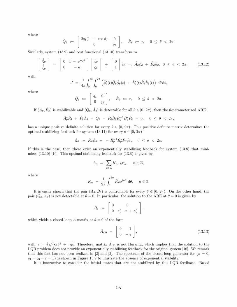
where
Qθ :=
[2q1(1 − cos θ) 0
0 q3
], Rθ := r, 0 ≤ θ < 2π.
Similarly, system (13.9) and cost functional (13.10) transform to[ ˙ηθ˙ζθ
]=
[0 1 − e−jθ
0 − κ
][ηθ
ζθ
]+
[01
]ˆuθ =: ˆAθφθ + ˆBθ ˆuθ, 0 ≤ θ < 2π, (13.12)
with
J =14π
∫ ∞
0
∫ 2π
0
(φ∗θ(t)
ˆQθφθ(t) + ˆu∗θ(t)Rθ ˆuθ(t))
dθ dt,
whereˆQθ :=
[q1 00 q3
], Rθ := r, 0 ≤ θ < 2π.
If (Aθ, Bθ) is stabilizable and (Qθ, Aθ) is detectable for all θ ∈ [0, 2π), then the θ-parameterized ARE
A∗θPθ + PθAθ + Qθ − PθBθR
−1θ B∗
θ Pθ = 0, 0 ≤ θ < 2π,
has a unique positive definite solution for every θ ∈ [0, 2π). This positive definite matrix determines theoptimal stabilizing feedback for system (13.11) for every θ ∈ [0, 2π)
ˆuθ := Kθψθ = − R−1θ B∗
θ Pθψθ, 0 ≤ θ < 2π.
If this is the case, then there exist an exponentially stabilizing feedback for system (13.8) that mini-mizes (13.10) [16]. This optimal stabilizing feedback for (13.8) is given by
un =∑k∈Z
Kn−kψk, n ∈ Z,
where
Kn =12π
∫ 2π
0
Kθejnθ dθ, n ∈ Z.
It is easily shown that the pair (Aθ, Bθ) is controllable for every θ ∈ [0, 2π). On the other hand, thepair (Qθ, Aθ) is not detectable at θ = 0. In particular, the solution to the ARE at θ = 0 is given by
P0 :=
[0 00 r(−κ + γ)
],
which yields a closed-loop A matrix at θ = 0 of the form
Acl0 =
[0 10 − γ
], (13.13)
with γ := 1r
√(κr)2 + rq3. Therefore, matrix Acl0 is not Hurwitz, which implies that the solution to the
LQR problem does not provide an exponentially stabilizing feedback for the original system [16]. We remarkthat this fact has not been realized in [2] and [3]. The spectrum of the closed-loop generator for κ = 0,q1 = q3 = r = 1 is shown in Figure 13.9 to illustrate the absence of exponential stability.
It is instructive to consider the initial states that are not stabilized by this LQR feedback. Based
192

-1.4 -1.2 -1 -0.8 -0.6 -0.4 -0.2 0 -1
-0.5
0
0.5
1
Re (λ Acl
)
Im ( λ
Acl
)
Figure 13.9: The spectrum of the closed-loop generator in an LQR controlled spatially invariant string ofvehicles (13.8) with performance objective (13.10) and κ = 0, q1 = q3 = r = 1.
on (13.13), it follows that the solution of system (13.11) at θ = 0 with the controller of [2] is determined by
ζ0(t) = e−γtζ0(0),
ξ0(t) = ξ0(0) − 1γ
(1 − e−γt)ζ0(0).
We have assumed that γ = 0, which can be accomplished for any κ ≥ 0 by choosing q3 > 0. Thus,
∑n∈Z
ξn(t) =∑n∈Z
ξn(0) − 1γ
(1 − e−γt)∑n∈Z
ζn(0),
which implies that limt→∞∑n∈Z
ξn(t) = 0 unless
∑n∈Z
ξn(0) − 1γ
∑n∈Z
ζn(0) ≡ 0. (13.14)
Therefore, if the initial condition of system (13.8) does not satisfy (13.14) than∑n∈Z
ξn(t) cannot beasymptotically driven towards zero. It is not difficult to construct a physically relevant initial condition thatviolates (13.14). For example, this situation will be encountered if the string of vehicles at t = 0 cruises atthe desired velocity vd with all the vehicles being at their desired spatial locations except for a single vehicle.In other words, even for a seemingly benign initial condition of the form ζn(0) ≡ 0; ξn(0) = 0, ∀n ∈Z \ 0; ξ0(0) = S = 0 there exist at least one vehicle whose absolute position error does not converge tozero as time goes to infinity when the control strategy of Melzer & Kuo [2] is employed. This non-zero meanposition initial condition is graphically illustrated in Figure 13.10.
Figure 13.10: An example of a position initial condition for which there is at least one vehicle whose absoluteposition error does not asymptotically converge to zero when the control strategy of [2] is used.
We note that system (13.12) is not stabilizable at θ = 0, which prevents system (13.9) from beingstabilizable [16]. Hence, when infinite vehicular platoons are considered the formulation of design problemof Levine & Athans [1] is ill-posed (that is, unstabilizable). In particular, the solution of the ‘η-subsystem’
193

of (13.12) at θ = 0 does not change with time, that is η0(t) ≡ η0(0), which indicates that∑n∈Z
ηn(t) ≡∑n∈Z
ηn(0). Therefore, for a non-zero mean initial condition ηn(0)n∈Z, the sum of all relative positionerrors is identically equal to a non-zero constant determined by
∑n∈Z
ηn(0). An example of such initialcondition is given by ηn(0) = 0, ∀n ∈ Z \ 0; η0(0) = S = 0, and it is illustrated in Figure 13.11. Itis quite remarkable that the control strategy of Levine & Athans [1] is not able to asymptotically steer allrelative position errors towards zero in an infinite platoon with this, at first glance, innocuously lookinginitial condition.
Figure 13.11: An example of a position initial condition for which there is at least a pair of vehicles whoserelative distance does not asymptotically converge to the desired inter-vehicular spacing L when a controlstrategy of [1] is used.
Therefore, we have shown that exponential stability of an LQR controlled infinite platoon cannot beachieved due to the lack of detectability (in the case of [2, 18]) and stabilizability (in the case of [1]). Thesefacts have very important practical implications for optimal control of large vehicular platoons. Namely,our analysis clarifies results of § 13.1.1, where we have observed that decay rates of a finite platoon withcontrollers of [1, 2, 18] become smaller as the platoon size increases.
In § 13.1.3, we demonstrate that exponential stability of an infinite string of vehicles can be guaran-teed by accounting for position errors with respect to absolute desired trajectories in both the state-spacerepresentation and the performance criterion.
13.1.3 Alternative problem formulations
In this subsection, we propose an alternative formulation of optimal control problems for vehicular platoons.In particular, we study distributed optimal control design with respect to quadratic performance criteria(LQR, H2, H∞), and show that the problems discussed in § 13.1.1 and § 13.1.2 can be overcome by accountingfor the absolute position errors in both the state-space realization and the performance criterion. We alsobriefly remark on the choice of the appropriate state-space.
Alternative LQR problem formulation
In this subsection, we suggest an alternative formulation of the LQR problem in order to overcome issuesraised in § 13.1.1 and § 13.1.2. Since consideration of infinite platoons is better suited for analysis, we firststudy the LQR problem for a spatially invariant string of vehicles, and then discuss practical implicationsfor optimal control of finite vehicular platoons.
We represent system shown in Figure 13.8 by its state-space representation (13.8) expressed in terms ofabsolute position and velocity error variables, and propose the quadratic performance objective of the form
J :=12
∫ ∞
0
∑n∈Z
(q1η
2n(t) + q2ξ
2n(t) + q3ζ
2n(t) + ru2
n(t))
dt
=12
∫ ∞
0
∑n∈Z
(q1(ξn(t) − ξn−1(t))2 + q2ξ
2n(t) + q3ζ
2n(t) + ru2
n(t))
dt,(13.15)
with q1, q2, q3, and r being positive design parameters. It should be noted that in (13.15) we account for bothabsolute position errors ξn and relative position errors ηn. This is in contrast to performance index (13.10)
194

considered by Melzer & Kuo [2] and Chu [3], where only relative position errors are penalized in J . The mainpoint of this subsection is to show that if one accounts for absolute position errors in the cost functional,then LQR feedback will be exponentially stabilizing.
Application of Zθ-transform renders (13.8) into (13.11), whereas (13.15) simplifies to
J =14π
∫ ∞
0
∫ 2π
0
(ψ∗θ(t)Q
θψθ(t) + ˆu∗θ(t)Rθ ˆuθ(t)
)dθ dt,
where
Qθ :=
[q2 + 2q1(1 − cos θ) 0
0 q3
], Rθ := r, 0 ≤ θ < 2π.
As shown in § 13.1.2, the pair (Aθ, Bθ) is controllable for every θ ∈ [0, 2π). Furthermore, it is easilyestablished that the pair (Qθ, Aθ) is detectable if and only if
q2 + 2q1(1 − cos θ) = 0, ∀ θ ∈ [0, 2π).
Even if q1 is set to zero, this condition is satisfied as long as q2 > 0. However, in this situation the inter-vehicular spacing is not penalized in the cost functional which may result into an unsafe control strategy.Because of that, as in [2, 3], we assign a positive value to q1. In this case, if q2 = 0, the pair (Qθ, Aθ) isnot detectable at θ = 0, which implies that accounting for the absolute position errors in the performancecriterion is essential for obtaining a stabilizing solution to the LQR problem. The spectrum of the closed-loopgenerator shown in Figure 13.12 illustrates exponential stability of infinite string of vehicles (13.8) combinedin feedback with a controller that minimizes performance objective (13.15) for κ = 0, q1 = q2 = q3 = r = 1.
-1.2 -1 -0.8 -0.6 -0.4 -0.2 0 -1
-0.5
0
0.5
1
Re (λ Acl
)
Im (λ
A
cl
)
Figure 13.12: The spectrum of the closed-loop generator in an LQR controlled spatially invariant string ofvehicles (13.8) with performance objective (13.15) and κ = 0, q1 = q2 = q3 = r = 1.
For a finite platoon with M vehicles the appropriately modified version of (13.15) is obtained by addingan additional term that accounts for absolute position errors to the right-hand side of (13.5)
J :=12
∫ ∞
0
(M+1∑n=1
q1η2n(t) +
M∑n=1
(q2ξ2n(t) + q3ζ2n(t) + ru2
n(t))
)dt
=12
∫ ∞
0
(M+1∑n=1
q1(ξn(t) − ξn−1(t))2 +M∑n=1
(q2ξ2n(t) + q3ζ2n(t) + ru2
n(t))
)dt.
(13.16)
Equivalently, (13.16) can be rewritten as
J =12
∫ ∞
0
(ψ∗(t)Qψ(t) + u∗(t)Ru(t)) dt,
195

where Q and R are 2M × 2M and M ×M matrices given by
Q :=[Q1 + q2I 0
0 q3I
], R := rI,
respectively. Toeplitz matrix Q1 has the same meaning as in § 13.1.1.The left and middle plots in Figure 13.13 respectively show the minimal and maximal eigenvalues of the
ARE solution for system (13.2) with performance objective (13.16), and the right plot in the same figureshows the real parts of the least-stable poles in an LQR controlled string of vehicles (13.2,13.16) for κ = 0,q1 = q2 = q3 = r = 1. Clearly, when the absolute position errors are accounted for in both the state-spacerealization and J , the problems addressed in § 13.1.1 are easily overcome. In particular, the least-stableclosed-loop eigenvalues converge towards a non-zero value determined by the dominant pole of the spatiallyinvariant system.
0 50 100 1500.72
0.74
0.76
0.78
0.8
0.82
0.84
M
λ min
P
M
0 50 100 1505.9
6
6.1
6.2
6.3
6.4
6.5
M
λ max
P
M
0 10 20 30 40 50 60 70 80 90
−0.94
−0.92
−0.9
−0.88
−0.86
M
max
Re
( λ
Acl
)
Figure 13.13: The minimal (left plot) and maximal eigenvalues (middle plot) of the ARE solution PM for sys-tem (13.2) with performance objective (13.16), and the dominant poles of LQR controlled platoon (13.2,13.16)(right plot) as functions of the number of vehicles, for κ = 0, q1 = q2 = q3 = r = 1.
Absolute position errors of an LQR controlled string (13.2,13.16) with 20 and 50 vehicles are shown inFigure 13.14. Simulation results are obtained for κ = 0, q1 = q2 = q3 = r = 1 and the initial conditionof the form ξn(0) = ζn(0) = 1, ∀n = 1, . . . ,M. These plots clearly demonstrate the uniform rate ofconvergence towards the desired formation. This is accomplished by expressing the state-space realizationin terms of the errors with respect to the absolute desired trajectories and by accounting for the absoluteposition errors in the performance objective.
M = 20: M = 50:
0 2 4 6 8 10−0.2
0
0.2
0.4
0.6
0.8
1
1.2
1.4
t
ξ n(t)
0 2 4 6 8 10−0.2
0
0.2
0.4
0.6
0.8
1
1.2
1.4
t
ξ n(t)
Figure 13.14: Absolute position errors of an LQR controlled string (13.2,13.16) with 20 vehicles (left plot)and 50 vehicles (right plot), for κ = 0, q1 = q2 = q3 = r = 1. Simulation results are obtained for thefollowing initial condition: ξn(0) = ζn(0) = 1, ∀n = 1, . . . ,M.
We note that qualitatively similar results are obtained if LQR problem is formulated for system (13.2)with either functional (13.6) or functional (13.7) augmented by a term penalizing absolute position errors.
196

Next, we formulate the distributed H2 and H∞ design problems for a spatially invariant string of vehicles,and discuss necessary conditions for the existence of stabilizing controllers.
H2 and H∞ control of spatially invariant vehicular platoons
In this subsection, we consider a spatially invariant string of vehicles shown in Figure 13.8 in the presenceof external disturbances
xn + κxn = un + dn, n ∈ Z, (13.17)
and formulate H2 and H∞ control problems. A disturbance acting on the n-th vehicle is denoted by dnand it can account for the external forces such as wind gusts, rolling resistance friction, pot holes, and non-horizontal road slopes. For simplicity, we assume that there are no model uncertainties and rewrite (13.17)in the form suitable for solving a standard robust control problem [19]
ψn = Aψn + B1wn + B2un
zn = C1ψn + D11wn + D12un
yn = C2ψn + D21wn + D22un
n ∈ Z, (13.18)
where
ψn :=
[ξn
ζn
], un := un − κvd, wn :=
[dn
νn
],
with νn denoting the measurement noise for the n-th vehicle. With these choices, matrices A, B1, and B2
are respectively determined by
A :=
[0 10 −κ
], B1 :=
[0 01 0
], B2 :=
[01
].
We further assume the ‘exogenous’ and ‘sensed’ outputs for the n-th vehicle of the form
zn :=
q1(ξn − ξn−1)
q2ξn
q3ζn
run
, yn := ξn + s1νn,
where q1, q2, q3, r, and s1 represent positive design parameters. Thus, operators Ci and Dij , for everyi, j = 1, 2 and n ∈ Z, are determined by
C1 :=
q1(1 − T−1) 0
q2 00 q3
0 0
, D11 := 0, D12 :=
000r
,
C2 :=[
1 0], D21 :=
[0 s1
], D22 := 0.
Application of Zθ-transform renders (13.18) into the θ-parameterized finite dimensional family of systems ofthe form
˙ψθ = Aθψθ + B1θwθ + B2θ
ˆuθzθ = C1θψθ + D11θwθ + D12θ
ˆuθyθ = C2θψθ + D21θwθ + D22θ
ˆuθ
θ ∈ [0, 2π), (13.19)
197

with
Aθ =
[0 10 −κ
], B1θ =
[0 01 0
], B2θ =
[01
],
C1θ =
q1(1 − e−jθ) 0
q2 00 q3
0 0
, D11θ = 0, D12θ =
000r
,
C2θ =[
1 0], D21θ =
[0 s1
], D22θ = 0.
Solving the distributed H2 and H∞ design problems for system (13.18) amounts to solving the H2 and H∞design problems for a parameterized family of finite dimensional LTI systems (13.19) over θ ∈ [0, 2π) [16].
The following properties of system (13.19) are readily established
1. Pairs (Aθ, B2θ) and (C2θ, Aθ) are respectively stabilizable and detectable for every θ ∈ [0, 2π).
2. D∗12θD12θ = r2 > 0, ∀ θ ∈ [0, 2π).
3. D21θD∗21θ = s21 > 0, ∀ θ ∈ [0, 2π).
4. D∗12θC1θ = 0, B1θD
∗21θ = 0, ∀ θ ∈ [0, 2π).
5. Pair (Aθ, B1θ) is stabilizable for every θ ∈ [0, 2π). Pair (C1θ, Aθ) is detectable for every θ ∈ [0, 2π) ifand only if q2 = 0.
If properties (4) and (5) hold than
σmin
[Aθ − jωI B2θ
C1θ D12θ
]≥ ε > 0, ∀ θ ∈ [0, 2π), ∀ω ∈ R, (13.20a)
σmin
[Aθ − jωI B1θ
C2θ D21θ
]≥ ε > 0, ∀ θ ∈ [0, 2π), ∀ω ∈ R, (13.20b)
which are necessary conditions for the existence of exponentially stabilizing solutions to these infinite dimen-sional H2 and H∞ control problems [16]. It is noteworthy that condition (13.20a) is going to be violatedunless q2 = 0. This further underlines the importance of incorporating the absolute position errors in theperformance objective.
Next, we briefly comment on the initial conditions that cannot be dealt with the quadratically optimalcontrollers of this subsection.
On the choice of the appropriate state-space
In this subsection, we remark on the initial conditions that are not square summable (in a space of theabsolute errors) and as such are problematic for optimal controllers involving quadratic criteria.
Motivated by example shown in Figure 13.11 we note that the initial relative position errors ηn(0)n∈Z
cannot be non-zero mean unless the absolute position errors at t = 0 sum to infinity. Namely, if∑n∈Z
ξn(0)is bounded, then∑
n∈Z
ηn(0) :=∑n∈Z
(ξn(0) − ξn−1(0)) =∑n∈Z
ξn(0) −∑n∈Z
ξn−1(0) = 0.
Clearly, for the initial condition shown in Figure 13.11, that is,
xn(0) = −nL + S, ∀n ∈ N0; xn(0) = −nL, ∀n ∈ Z \ N0,
198

sequence ξn(0)n∈Z sums to infinity if S = 0. In addition to that, ξn(0)n∈Z /∈ l2, whereas ηn(0)n∈Z
∈ l2. Therefore, despite the fact that the inter-vehicular spacing for all but a single vehicle is kept at thedesired level L, a relevant non-square summable initial condition1 is easily constructed. It is worth notingthat LQR, H2, and H∞ controllers of § 13.1.3 are derived under the assumption of the square summableinitial conditions and as such cannot be used for guarding against an entire class of physically relevant initialstates. This illustrates that a Hilbert space l2 may represent a rather restrictive choice for the underlyingstate-space of system (13.8). Perhaps the more appropriate state-space for this system is a Banach spacel∞. The control design on this state-space is discussed in § 13.2.
13.2 Limitations and tradeoffs in the control of vehicular platoons
In this section, we study some fundamental limitations and tradeoffs in the control of vehicular platoons.We illustrate that in very long platoons one needs to account explicitly for the initial distances of vehiclesfrom their desired trajectories in order to avoid large position and velocity deviations and the excessive useof control effort. We further derive an initial condition dependent set of requirements that the control gainsneed to satisfy to guarantee the desired quality of position transient response, and rule out saturation inboth velocity and control. These requirements are used to generate the trajectories around which the statesof the string of vehicles are driven to their desired values without the excessive use of control effort.
Our presentation is organized as follows: in § 13.2.1, we propose a distributed control strategy thatprovides stability of an infinite dimensional platoon system. In § 13.2.2, we illustrate that commanding auniform rate of convergence for all vehicles towards their desired trajectories may require large control efforts.In § 13.2.3, we remark on some basic design limitations and tradeoffs in vehicular platoons and determinethe conditions that control gains need to satisfy to provide operation within the imposed saturation limits.In § 13.2.4, we redesign the controller of § 13.2.1 to provide the desired quality of transient response andavoid large control excursions.
13.2.1 Lyapunov-based control of vehicular platoons
A system of identical unit mass vehicles in a semi-infinite string is shown in Figure 13.15.
Figure 13.15: Semi-infinite platoon of vehicles. The lead vehicle is indexed by zero.
For notational convenience, we do not include the air resistance force in the model (i.e., set κ to 0in (13.1)) which yields
xn = un, n ∈ N0, (13.21)
where N0 := 0 ∪ N = 0, 1, 2, . . .. A control objective the same as in § 13.1: to provide a desired constantcruising velocity vd and to keep the inter-vehicular distance at a constant pre-specified level L. A coordinatetransformation of the form
en(t) := αnξn(t) + βnηn(t), n ∈ N0, (13.22)
1In a space of the absolute position errors.
199

renders (13.21) intoφn = ψn
ψn = −βnun−1 + (αn + βn)un
n ∈ N0, (13.23)
where αn and βn represent nonnegative parameters that are not simultaneously equal to zero, with β0 ≡ 0,and φn := en, ψn := en. On the other hand, ξn and ηn respectively denote the previously defined (see§ 13.1.1) position error variables of the n-th vehicle with respect to the absolute and relative reference frames:
ξn(t) := xn(t) − vdt + nL, n ∈ N0
ηn(t) := xn(t) − xn−1(t) + L, n ∈ N.
By assigning different values to αn and βn we can adjust the relative importance of these two quantities.The appropriate state-space for system (13.23) is a Banach space l∞× l∞. This choice of the state-space
implies that initially, at t = 0, no vehicle is infinitely far from its desired absolute position. Control designshould provide boundedness of position and velocity error variables for every t > 0 and their asymptoticconvergence to zero. In § 13.2.2, we illustrate, by means of an example, that choosing a Hilbert space l2 × l2rather than a Banach space l∞ × l∞ for the underlying state-space can be rather restrictive. Namely, thischoice of the state-space can exclude an entire set of relevant initial conditions from the analysis.
In particular, a choice of control law of the form
un =βn
αn + βnun−1 −
1αn + βn
(anφn + bnψn), (13.24)
with an > 0, bn > 0, ∀n ∈ N0, yields an infinite number of stable, fully decoupled second order subsystems
φn = ψn
ψn = − anφn − bnψn
n ∈ N0. (13.25)
Therefore, we conclude boundedness of both en(t) and en(t), ∀ t ≥ 0, and their asymptotic convergence tozero, for every n ∈ N0.
In the remainder of this subsection, we assume that αn := α = const., βn := β = const., ∀n ∈ N;α0 = 0, β0 ≡ 0. In this case, controller (13.24) simplifies to
u0 = − 1α0
(a0φ0 + b0ψ0), (13.26a)
un =β
α+ βun−1 − 1
α+ β(anφn + bnψn), n ∈ N,
which in turn implies
un =βn
(α+ β)nu0 −
n∑k=1
βn−k
(α+ β)n−k+1(akφk + bkψk), (13.27)
for every n ∈ N. If α = 0, β = 0, controller (13.26a,13.27) does not take information about the precedingvehicle into consideration since it only accounts for the error variable with respect to the absolute desiredtrajectory. Therefore, this control strategy is unsafe and because of that we choose β = 0. On the otherhand, if α = 0, β = 0, the information about all vehicles enters into (13.27) with the same importancewhich is not desirable from communication point of view. For these reasons, we consider the situation inwhich both α and β have positive values and rewrite (13.27) as
un = qnu0 −1β
n∑k=1
qn−k+1(akφk + bkψk), n ∈ N, (13.28)
where q := β/(α + β) < 1. With this choice of design parameters α and β the gains in (13.28) decay
200
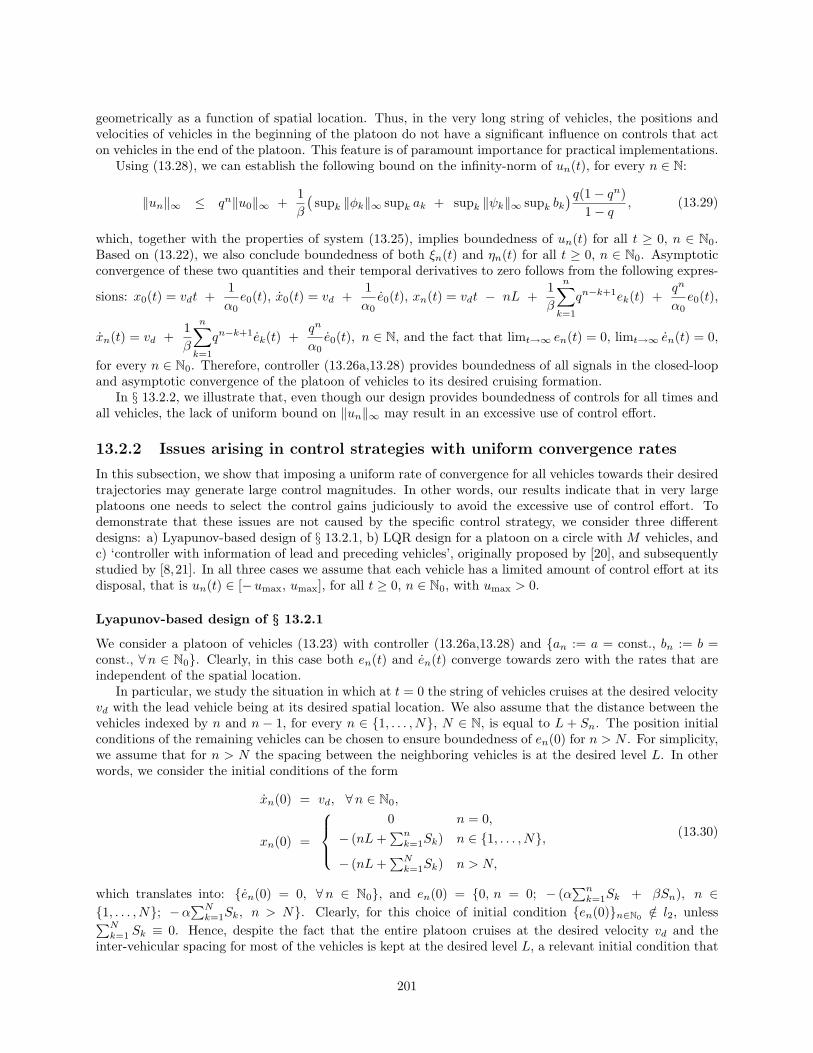
geometrically as a function of spatial location. Thus, in the very long string of vehicles, the positions andvelocities of vehicles in the beginning of the platoon do not have a significant influence on controls that acton vehicles in the end of the platoon. This feature is of paramount importance for practical implementations.
Using (13.28), we can establish the following bound on the infinity-norm of un(t), for every n ∈ N:
‖un‖∞ ≤ qn‖u0‖∞ +1β
(supk ‖φk‖∞ supk ak + supk ‖ψk‖∞ supk bk
)q(1 − qn)1 − q
, (13.29)
which, together with the properties of system (13.25), implies boundedness of un(t) for all t ≥ 0, n ∈ N0.Based on (13.22), we also conclude boundedness of both ξn(t) and ηn(t) for all t ≥ 0, n ∈ N0. Asymptoticconvergence of these two quantities and their temporal derivatives to zero follows from the following expres-
sions: x0(t) = vdt +1α0e0(t), x0(t) = vd +
1α0e0(t), xn(t) = vdt − nL +
1β
n∑k=1
qn−k+1ek(t) +qn
α0e0(t),
xn(t) = vd +1β
n∑k=1
qn−k+1ek(t) +qn
α0e0(t), n ∈ N, and the fact that limt→∞ en(t) = 0, limt→∞ en(t) = 0,
for every n ∈ N0. Therefore, controller (13.26a,13.28) provides boundedness of all signals in the closed-loopand asymptotic convergence of the platoon of vehicles to its desired cruising formation.
In § 13.2.2, we illustrate that, even though our design provides boundedness of controls for all times andall vehicles, the lack of uniform bound on ‖un‖∞ may result in an excessive use of control effort.
13.2.2 Issues arising in control strategies with uniform convergence rates
In this subsection, we show that imposing a uniform rate of convergence for all vehicles towards their desiredtrajectories may generate large control magnitudes. In other words, our results indicate that in very largeplatoons one needs to select the control gains judiciously to avoid the excessive use of control effort. Todemonstrate that these issues are not caused by the specific control strategy, we consider three differentdesigns: a) Lyapunov-based design of § 13.2.1, b) LQR design for a platoon on a circle with M vehicles, andc) ‘controller with information of lead and preceding vehicles’, originally proposed by [20], and subsequentlystudied by [8,21]. In all three cases we assume that each vehicle has a limited amount of control effort at itsdisposal, that is un(t) ∈ [−umax, umax], for all t ≥ 0, n ∈ N0, with umax > 0.
Lyapunov-based design of § 13.2.1
We consider a platoon of vehicles (13.23) with controller (13.26a,13.28) and an := a = const., bn := b =const., ∀n ∈ N0. Clearly, in this case both en(t) and en(t) converge towards zero with the rates that areindependent of the spatial location.
In particular, we study the situation in which at t = 0 the string of vehicles cruises at the desired velocityvd with the lead vehicle being at its desired spatial location. We also assume that the distance between thevehicles indexed by n and n − 1, for every n ∈ 1, . . . , N, N ∈ N, is equal to L + Sn. The position initialconditions of the remaining vehicles can be chosen to ensure boundedness of en(0) for n > N . For simplicity,we assume that for n > N the spacing between the neighboring vehicles is at the desired level L. In otherwords, we consider the initial conditions of the form
xn(0) = vd, ∀n ∈ N0,
xn(0) =
0 n = 0,− (nL+
∑nk=1Sk) n ∈ 1, . . . , N,
− (nL+∑Nk=1Sk) n > N,
(13.30)
which translates into: en(0) = 0, ∀n ∈ N0, and en(0) = 0, n = 0; − (α∑nk=1Sk + βSn), n ∈
1, . . . , N; −α∑Nk=1Sk, n > N. Clearly, for this choice of initial condition en(0)n∈N0 /∈ l2, unless∑N
k=1 Sk ≡ 0. Hence, despite the fact that the entire platoon cruises at the desired velocity vd and theinter-vehicular spacing for most of the vehicles is kept at the desired level L, a relevant initial condition that
201
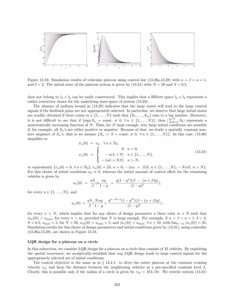
0 2 4 6 8 10
−25
−20
−15
−10
−5
0
t
ξ n(t)
0 2 4 6 8 10
0
2
4
6
8
10
t
dξn(t)
/dt
0 2 4 6 8 100
5
10
15
20
25
t
u n(t)
Figure 13.16: Simulation results of vehicular platoon using control law (13.26a,13.28) with α = β = a = 1,and b = 2. The initial state of the platoon system is given by (13.31) with N = 50 and S = 0.5.
does not belong to l2 × l2 can be easily constructed. This implies that a Hilbert space l2 × l2 represents arather restrictive choice for the underlying state-space of system (13.23).
The absence of uniform bound in (13.29) indicates that the large states will lead to the large controlsignals if the feedback gains are not appropriately selected. In particular, we observe that large initial statesare readily obtained if there exists m ∈ 1, . . . , N such that S1, . . . , Sm sum to a big number. Moreover,it is not difficult to see that if signSn = const. = 0, ∀n ∈ 1, . . . , N, then |∑N
k=1 Sk| represents amonotonically increasing function of N . Thus, for N large enough, very large initial conditions are possibleif, for example, all Sn’s are either positive or negative. Because of that, we study a spatially constant non-zero sequence of Sn’s, that is we assume Sn := S = const. = 0, ∀n ∈ 1, . . . , N. In this case, (13.30)simplifies to
xn(0) = vd, ∀n ∈ N0,
xn(0) =
0 n = 0,−n(L+ S) n ∈ 1, . . . , N,
− (nL+NS) n > N,
(13.31)
or equivalently en(0) = 0, ∀n ∈ N0, en(0) = 0, n = 0; − (nα + β)S, n ∈ 1, . . . , N; −NαS, n > N.For this choice of initial conditions u0 ≡ 0, whereas the initial amount of control effort for the remainingvehicles is given by
un(0) =aS
β(n
αq
1 − q+
q(1 − qn)(β − (α+ β)q)(1 − q)2
),
for every n ∈ 1, . . . , N, and
un(0) =aS
β(Nαq
1 − q+qn−N+1(1 − qN )(β − (α+ β)q)
(1 − q)2),
for every n > N , which implies that for any choice of design parameter a there exist m ∈ N such that|un(0)| > umax, for every n > m, provided that N is large enough. For example, if α = β = a = 1, b = 2,S = 0.5, umax = 5, for N = 50, u10(0) = umax = 5, and |un(0)| > umax, ∀n > 10, with limn→∞ |un(0)| = 25.Simulation results for this choice of design parameters and initial conditions given by (13.31), using controller(13.26a,13.28), are shown in Figure 13.16.
LQR design for a platoon on a circle
In this subsection, we consider LQR design for a platoon on a circle that consists of M vehicles. By exploitingthe spatial invariance, we analytically establish that any LQR design leads to large control signals for theappropriately selected set of initial conditions.
The control objective is the same as in § 13.2.1: to drive the entire platoon at the constant cruisingvelocity vd, and keep the distance between the neighboring vehicles at a pre-specified constant level L.Clearly, this is possible only if the radius of a circle is given by rM = ML/2π. We rewrite system (13.21)
202

Figure 13.17: Circular platoon of M vehicles.
for n ∈ 0, . . . ,M − 1 in terms of a state-space realization of the form[ξnςn
]=
[0 10 0
] [ξnςn
]+
[01
]un
=: Anϕn + Bnun,(13.32)
where ξn(t) := xn(t) − vdt − nL and ςn(t) := xn(t) − vd denote the absolute position and velocity errors ofthe n-th vehicle, respectively. We propose the following cost functional
J :=12
∫ ∞
0
M−1∑n=0
M−1∑m=0
(ϕ∗n(t)Qn−mϕm(t) + u∗n(t)Rn−mum(t)) dt, (13.33)
whereM−1∑n=0
M−1∑m=0
ϕ∗nQn−mϕm ≥ 0, Q∗
−n = Qn,
for all sequences ϕn, andM−1∑n=0
M−1∑m=0
u∗nRn−mum > 0, R∗−n = Rn,
for all non-zero sequences un.We utilize the fact that system (13.32) has spatially invariant dynamics over a circle. This implies that the
Discrete Fourier Transform (DFT) can be used to convert analysis and quadratic design problems into thosefor a parameterized family of second order systems [16]. DFT is defined by: xk := 1√
M
∑M−1n=0 xne−i 2πnk
M ,
k ∈ 0, . . . ,M − 1, and the inverse DFT is defined by: xn := 1√M
∑M−1k=0 xkei 2πnk
M , n ∈ 0, . . . ,M − 1.Using this, system (13.32) and quadratic performance index (13.33) transform to[
˙ξk˙ςk
]=
[0 10 0
] [ξkςk
]+
[01
]uk
=: Akϕk + Bkuk, k ∈ 0, . . . ,M − 1,(13.34)
and
J =√M
2
M−1∑k=0
∫ ∞
0
(ϕ∗k(t)Qkϕk(t) + u∗k(t)Rkuk(t)
)dt,
where Rk > 0 and
Qk :=
[q11k q∗21kq21k q22k
]≥ 0,
for every k ∈ 0, . . . ,M − 1. Clearly, the pair (Ak, Bk) is stabilizable for every k ∈ 0, . . . ,M − 1.On the other hand, the pair (Qk, Ak) is detectable if and only if q11k > 0 for every k ∈ 0, . . . ,M − 1.These conditions are necessary and sufficient for the existence of a stabilizing optimal solution to the LQRproblem (13.32,13.33). For additional information about proper formulation of quadratically optimal (i.e.,
203

LQR, H2, H∞) distributed control problems for large-scale and infinite vehicular platoons, we refer thereader to § 13.1.3..
It is readily shown that for xn(0) ≡ vd, i.e. for ςn(0) ≡ 0, we have:
M−1∑n=0
u2n(0) =
M−1∑k=0
q11k
Rkξ∗k(0)ξk(0),
which in turn implies
infk
q11k
Rk
M−1∑n=0
ξ2n(0) ≤M−1∑n=0
u2n(0) ≤ sup
k
q11k
Rk
M−1∑n=0
ξ2n(0).
Thus, we have established the lower and upper bounds on the initial amount of control effort for a formationthat cruises at the desired velocity vd. These bounds are determined by the deviations of vehicles fromtheir absolute desired trajectories at t = 0, and by the LQR design parameters q11k and Rk. Clearly, sinceq11k > 0 (for detectability) infk q11k/Rk is always greater than zero. We note that this quantity can be madesmaller by increasing the control penalty. In particular, for xn(0) = n(L− S), 0 < S < L, we have
M−1∑n=0
u2n(0) ≥ S2
6M(M − 1)(2M − 1) inf
k
q11k
Rk,
which illustrates an unfavorable scaling of the initial amount of control effort with the number of vehiclesin formation. Hence, unless umax ≥ S2(M − 1)(2M − 1) infk q11k/6Rk, there exist at least one vehicle forwhich |un(0)| > umax.
Controller of [20]
In this subsection, we show that the controller of [20] faces the very same issues as the previously discussedcontrol strategies with uniform convergence rates. We study this controller because of its superior propertiescompared to other ‘look-ahead vehicle following algorithms’ (see Table 1 of [8] for comparison of differentconstant spacing platoon strategies).
Controller of [20] for system (13.21) is, for any n ∈ N, given by (see § 3.4 of [8]):
un =1
1 + q3
(xn−1 + q3x0 − (q1 + λ)ηn − q1ληn − (q4 + λq3)(xn − x0) − λq4(xn − x0 + nL)
),
where q1, q3, q4, and λ represent positive design parameters, whereas the lead vehicle is indexed by 0.Equivalently, un is determined by the following recursive relation
un = (1 − )u0 + un−1 − fn, n ∈ N, (13.35)
where
fn := (q1 + λ)ηn + q1ληn + (q4 + λq3)n∑k=1
ηk + λq4
n∑k=1
ηk
= (q1 + λ)(ξn − ξn−1) + q1λ(ξn − ξn−1) + (q4 + λq3)(ξn − ξ0) + λq4(ξn − ξ0),
and := 1/(1 + q3) < 1. Finally, using (13.35) we express un as
un = u0 −n∑k=1
n−k+1fk, n ∈ N.
In particular, for initial condition (13.31), or equivalently ξn(0) = 0, ∀n ∈ N0, ξn(0) = 0, n = 0; −nS, n ∈1, . . . , N; −NS, n > N, u0 is identically equal to 0. On the other hand, the initial amount of control
204

effort for the remaining vehicles is given by
un(0) = λS(nq4
1 − +
q1(1 − n)1 −
− q42(1 − n)
(1 − )2),
for every n ∈ 1, . . . , N, and
un(0) = λS(Nq4(1 + N − n)
1 − +
q1(1 − N )1 −
− q42(1 − N )(1 − )2
),
for every n > N . Thus, for any choice of design parameters q1, q3, q4, and λ there exist m ∈ N such that|un(0)| > umax, for every n > m, provided that N is large enough.
The results of this subsection illustrate that in very large platoons one needs to take into account theinitial distance of vehicles from their desired trajectories and to adjust the control gains accordingly in orderto avoid large velocity deviations and the excessive use of control effort. In the next subsection, we giveconditions that the feedback gains need to satisfy to prevent saturation in both velocity and control anddiscuss some design limitations and tradeoffs in vehicular platoons.
13.2.3 Design limitations and tradeoffs in vehicular platoons
In this subsection, we determine the conditions that control gains need to satisfy to provide operation withinthe imposed saturation limits. Our analysis yields the explicit constraints on these gains−for any given setof initial conditions−to achieve desired position transients without magnitude and rate saturation. We alsoremark on some of the basic limitations and tradeoffs that need to be addressed in the control of vehicularplatoons.
We rewrite system (13.21) as¨xn = un, n ∈ N0. (13.36)
The justification for the notation used in (13.36) is given in § 13.2.4. We want to drive each vehicle towardsits desired absolute position vdt− nL, and its desired velocity vd. For the time being we are not concernedwith the relative spacing between the vehicles. If we introduce the error variable rn(t) := xn(t) − vdt + nL,n ∈ N0, we can rewrite (13.36) as
rn = un, n ∈ N0, (13.37)
and choose un to meet the control objective. In particular, we take un of the form
un = − p2nrn − 2pnrn, n ∈ N0, (13.38)
where, for every n ∈ N0, pn represents a positive design parameter. With this choice of control, the solutionof system (13.37,13.38) is for any n ∈ N0 given by
rn(t) = (cn + dnt)e−pnt, (13.39a)
rn(t) = (dn − cnpn − dnpnt)e−pnt, (13.39b)
un(t) = (cnp2n − 2dnpn + dnp
2nt)e
−pnt, (13.39c)
where for every n ∈ N0
cn := rn(0) = xn(0) + nL,dn := rn(0)pn + rn(0)
= (xn(0) + nL)pn + ( ˙xn(0) − vd).(13.40)
We want to determine conditions that the sequence of positive numbers pnn∈N0 has to satisfy to
205

guarantee
|rn(t)| ≤ rn,max, ∀ t ≥ 0, (13.41a)|rn(t)| ≤ vmax, ∀ t ≥ 0, (13.41b)|un(t)| ≤ umax, ∀ t ≥ 0, (13.41c)
with rn,max > 0, ∀n ∈ N0, vmax > 0, and umax > 0 being the pre-specified numbers. For notationalconvenience, we have assumed that all vehicles have the same velocity and control saturation limits, givenby vmax and umax, respectively. Typically, the sequence rn,maxn∈N0 is given in terms of position initialconditions rn(0)n∈N0 as rn,max := γn|rn(0)|n∈N0 , where sequence of numbers γn > 1, ∀n ∈ N0determines the allowed overshoot with respect to the desired position trajectory of the n-th vehicle. Clearly,for this choice of rn,maxn∈N0 , rn(0)n∈N0 satisfies (13.41a). Based on (13.39a), rn(t) asymptotically goesto zero, so we only need to determine conditions under which (13.41a) is violated for finite non-zero times.If (13.39a) achieves an extremum for some tn ∈ (0, ∞), the absolute value of rn at that point is given by:
|rn(tn)| =|dn|pn
e−pn tn ≤ |dn|pn
≤ |rn(0)|pn
+ |rn(0)|.
Therefore, if sequence of positive numbers pnn∈N0 is chosen such that
|rn(0)|pn
+ |rn(0)| ≤ rn,max, ∀n ∈ N0, (13.42)
condition (13.41a) will be satisfied for every t ≥ 0. This implies that, for good position transient response(that is, for small position overshoots), design parameters pn have to assume large enough values determinedby (13.42).
Clearly, (13.41b) is going to be violated unless |rn(0)| ≤ vmax, for every n ∈ N0. If rn has a maximumor a minimum at some non-zero finite time tn, the absolute value of (13.39b) at that point can be upperbounded by
|rn(tn)| = |dn|e−pn tn ≤ |dn| ≤ |rn(0)|pn + |rn(0)|.Thus, to avoid velocity saturation, sequence of positive design parameters pnn∈N0 has to be small enoughto satisfy
|rn(0)|pn + |rn(0)| ≤ vmax, ∀n ∈ N0. (13.43)
Finally, to rule out saturation in control we need to make sure that condition (13.41c) is satisfied for botht = 0 and tn > 0, where the potential extremum of un takes place. The absolute values of (13.39c) at thesetwo time instants are respectively given by |un(0)| = |− rn(0)p2
n − 2rn(0)pn| ≤ |rn(0)|p2n + 2|rn(0)|pn, and
|un(tn)| = |dn|pne−pn tn ≤ |dn|pn ≤ |rn(0)|p2n + |rn(0)|pn. Since pn > 0, for every n ∈ N0, condition (13.41c)
is met if|rn(0)|p2
n + 2|rn(0)|pn ≤ umax, ∀n ∈ N0. (13.44)
Inequalities (13.42), (13.43), and (13.44) establish conditions for positive design parameters pn to preventsaturation in velocity and control, and guarantee a good position transient response. We remark that theseconditions can be somewhat conservative, but they are good enough to illustrate the major point. Clearly, forsmall excursions from the desired position trajectories control gains have to assume large values, determinedby (13.42). On the other hand, for small velocity deviations and small control efforts these gains have to besmall enough to satisfy (13.43) and (13.44). These facts illustrate some basic tradeoffs that designer facesin the control of vehicular platoons. In particular, the set of control gains that satisfies (13.43) and (13.44)determines the maximal position deviations and the rates of convergence towards the desired trajectories.In other words, the position overshoots and settling times can be significantly increased in the presence ofstringent requirements on velocity and control saturation limits.
206

0 10 20 30 40 50 60
−25
−20
−15
−10
−5
0
t
r n(t)
0 10 20 30 40 50 60
0
0.5
1
1.5
2
t
drn(t)
/dt
0 10 20 30 40 50 60−1
0
1
2
3
4
t
u n(t)
0 20 40 60 80 1000
0.5
1
1.5
2
2.5
3
n
p n
Figure 13.18: Solution of system (13.37,13.38) for initial conditions determined by (13.45) with N = 50 andSn = 0.5, for every n ∈ 1, . . . , N. The control gains are determined using (13.46) with vmax = umax = 5,and n = 1, σn = 0.8, ∀n ∈ N.
For the example considered in § 13.2.2 with the initial conditions of the form
˙xn(0) = vd, ∀n ∈ N0,
xn(0) =
0 n = 0,− (nL+
∑nk=1Sk) n ∈ 1, . . . , N,
− (nL+∑Nk=1Sk) n > N,
(13.45)
condition (13.42) is always satisfied, which implies that the largest deviation for all vehicles from theirdesired absolute positions takes place at t = 0. Therefore, the chosen initial conditions do not imposeany lower bounds on the control gains. On the other hand, whereas conditions (13.43) and (13.44) donot put any constraints on p0, they respectively dictate the following upper bounds on pnn∈N: pn ≤vmax/|
∑nk=1Sk|, n ∈ 1, . . . , N; vmax/|
∑Nk=1Sk|, n > N, and pn ≤
√umax/|
∑nk=1Sk|, n ∈ 1, . . . , N;√
umax/|∑Nk=1Sk|, n > N. In particular, the following choice of pnn∈N
pn =
min
nvmax
|∑nk=1Sk|
,
√σnumax
|∑nk=1Sk|
n < N,
min
nvmax
|∑Nk=1Sk|
,√ σnumax
|∑Nk=1Sk|
n ≥ N,
(13.46)
with 0 < n ≤ 1, 0 < σn ≤ 1, ∀n ∈ N, clearly satisfies the above requirements. Figure 13.18 illustratesthe solution of system (13.37,13.38) for initial conditions determined by (13.45) with N = 50 and Sn = 0.5,for every n ∈ 1, . . . , N. The control gains are chosen using (13.46) with vmax = umax = 5, n = 1, σn =0.8, ∀n ∈ N, to prevent reaching imposed velocity and control saturation limits. The dependence of thesegains on discrete spatial variable n is also illustrated in Figure 13.18.
Thus we have shown that controller (13.38) with the gains satisfying (13.42), (13.43), and (13.44) pre-
207
cludes saturation in both velocity and control and takes into account the desired quality of position transientresponse. However, this control strategy is unsafe, since it does not account for the inter-vehicular spacings.Because of that, in § 13.2.4 we redesign controller (13.26a,13.27) by incorporating the constraints imposedby (13.41) in the synthesis.
13.2.4 Control without reaching saturation
We again consider system (13.21), and introduce an error variable of the form
εn(t) := αnζn(t) + βnχn(t), n ∈ N0, (13.47)
where: ζn(t) := xn(t) − vdt + nL − rn(t) = ξn(t) − rn(t), n ∈ N0, χn(t) := ζn(t) − ζn−1(t) =xn(t) − xn−1(t) + L − rn(t) + rn−1(t), n ∈ N, with rn(t) being defined by (13.39a,13.40), pnn∈N0
satisfying (13.42), (13.43), and (13.44), and parameters αnn∈N0 and βnn∈N0 having the properties dis-cussed in § 13.2.1. The initial conditions on these two variables and their first derivatives are given by:ζn(0) = xn(0) − xn(0) =: µn, n ∈ N0, ζn(0) = xn(0) − ˙xn(0) =: νn, n ∈ N0, χn(0) = ζn(0) −ζn−1(0) = µn − µn−1, n ∈ N, χn(0) = ζn(0) − ζn−1(0) = νn − νn−1, n ∈ N, where xn(0), xn(0)n∈N0
and xn(0), ˙xn(0)n∈N0 represent the actual and the measured initial conditions, respectively. If perfectinformation about the initial positions and velocities is available, then clearly µn = νn = 0, ∀n ∈ N0.However, since initial condition uncertainties are always present we want to design a controller to guardagainst them.
Double differentiation of (13.47) with respect to time yields
εn = (αn + βn)(un − un) − βn(un−1 − un−1)=: (αn + βn)un − βnun−1, n ∈ N0,
(13.48)
where un is given by (13.38). System (13.48) can be represented in terms of its state-space realization of theform
ϑn = υn
υn = −βnun−1 + (αn + βn)un
n ∈ N0, (13.49)
where ϑn := εn, υn := εn. In particular, this system can be stabilized by the following feedback
u0 = − 1α0
(a0ϑ0 + b0υ0), (13.50a)
un = u0
n∏k=1
qk −n∑k=1
1βk
(akϑk + bkυk)n∏i=k
qi, (13.50b)
with qk := βk/(αk + βk), provided that βn = 0, ∀n ∈ N. It is noteworthy that, if parameters αn and βnare such that αn := α = const., βn := β = const., ∀n ∈ N, then controller (13.50) has the same propertiesas controller (13.26a,13.27). For the same choices of design parameters ann∈N0 and bnn∈N0 , these twocontrol strategies are only distinguished by the regions from where the states of systems (13.23) and (13.49)have to be brought to the origin. Namely, due to different formulations of control objectives, the initial statesof system (13.23) may occupy a portion of the state-space that is significantly larger than a region to whichthe initial conditions of system (13.49) belong. In the former case, this region is determined by the maximaldeviations from the desired absolute trajectories at t = 0, whereas, in the latter case, it is determined bythe precision of measurement devices, that is their ability to yield an accurate information about the initialpositions and velocities. As illustrated in § 13.2.2, the initial conditions may have an unfavorable scaling withdiscrete spatial variable n, which may result in the very large initial position deviations (and consequently,a large amount of the initial control effort) for large n’s, unless the size of the initial conditions is explicitlyaccounted for. We have shown in § 13.2.3 how to generate the initial condition dependent trajectories aroundwhich the states of vehicular platoon can be driven to zero without extensive use of control effort and largeposition and velocity overshoots.
208

0 10 20 30 40 50 60
−25
−20
−15
−10
−5
0
t
ξ n(t)
0 10 20 30 40 50 60−0.5
0
0.5
1
1.5
2
t
dξn(t)
/dt
0 10 20 30 40 50 60−1
0
1
2
3
4
5
t
u n(t)
Figure 13.19: Simulation results of platoon with 101 vehicles (M = 100) using controller (13.51) with α0 = 1,αn = βn = 1, ∀n ∈ 1, . . . ,M, an = 1, bn = 2, ∀n ∈ 0, . . . ,M. The measured initial condition isgiven by (13.45) with N = 50 and Sn = 0.5, for every n ∈ 1, . . . , N, whereas the numbers µn and νn thatdetermine the actual initial condition are randomly selected.
Using the definition of un, we finally give the expressions for unn∈N0
un = un + un, (13.51)
where un and un are respectively given by (13.38) and (13.50). We remark that un ≡ un, ∀n ∈ N0 ifperfect information about the initial conditions is available. The only role of unn∈N0 is to account for thediscrepancies in the initial conditions due to measurement imperfections.
Asymptotic convergence of ζn, χn, ζn, and χn to the origin for every n ∈ N0 can be easily established.Therefore, controller (13.51) provides operation within the imposed saturation bounds and asymptotic con-vergence of the platoon of vehicles to its desired cruising formation.
Simulation results of the platoon system with 101 vehicles (M = 100) using controller (13.51) withα0 = 1, αn = βn = 1, ∀n ∈ 1, . . . ,M, an = 1, bn = 2, ∀n ∈ 0, . . . ,M are shown in Figure 13.19.The measured initial condition is given by (13.45) with N = 50 and Sn = 0.5, for every n ∈ 1, . . . , N,whereas the numbers µn and νn that determine the actual positions and velocities at t = 0 are randomlyselected. The rates of convergence towards the origin are chosen using (13.46) with vmax = umax = 5,n = 1, σn = 0.8, ∀n ∈ 1, . . . ,M, to prevent reaching imposed velocity and control saturation limits,and p0 is set to 1. These convergence rates are shown in the far right plot in Figure 13.18. Clearly, thedesired control objective is successfully accomplished with the quality of the transient response determinedby the prescribed saturation bounds.
13.3 Summary
In this chapter, we have illustrated potential difficulties in the control of large or infinite vehicular platoons.In particular, shortcomings of previously reported solutions to the LQR problem have been exhibited. Byconsidering the case of infinite platoons as the limit of the large-but-finite case, we have shown analyticallyhow the aforementioned formulations lack stabilizability or detectability. We have argued that the infinitecase is a useful abstraction of the large-but-finite case, in that it explains the almost loss of stabilizabilityor detectability in the large-but-finite case, and the arbitrarily slowing rate of convergence towards desiredformation observed in numerical studies of finite platoons of increasing sizes. Finally, using the infinite pla-toon formulation, we have shown how incorporating absolute position errors in the cost functional alleviatesthese difficulties and provides uniformly bounded rates of convergence. It is noteworthy that the early workof [1–3, 18] is very widely cited, but to our knowledge these serious difficulties with their methods have notbeen previously pointed out in the literature.
We have further shown that imposing a uniform rate of convergence for all vehicles towards their de-sired trajectories may generate large control magnitudes for certain physically realistic initial conditions.Therefore, even though the formulation of an optimal control problem suggested in § 13.1.3 circumvents theweak points of [1–3, 18], additional care should be exercised in control of vehicular platoons (as illustrated
209

in § 13.2). Namely, we have demonstrated that in very large platoons the designer needs to pay attention tothe initial deviations of vehicles from their desired trajectories when selecting control gains. We have alsoestablished explicit constraints on these gains–for any given set of initial conditions–to assure the desiredquality of position transients without magnitude and rate saturation. These requirements have been usedto generate the trajectories around which the states of the platoon system are driven towards their desiredvalues without the excessive use of control effort.
210

Bibliography
[1] W. S. Levine and M. Athans, “On the optimal error regulation of a string of moving vehicles,” IEEETransactions on Automatic Control, vol. AC-11, no. 3, pp. 355–361, July 1966.
[2] S. M. Melzer and B. C. Kuo, “Optimal regulation of systems described by a countably infinite numberof objects,” Automatica, vol. 7, pp. 359–366, 1971.
[3] K. C. Chu, “Decentralized control of high-speed vehicular strings,” Transportation Science, vol. 8, no. 4,pp. 361–384, November 1974.
[4] S. Shladover, C. Desoer, J. Hedrick, M. Tomizuka, J. Walrand, W.-B. Zhang, D. McMahon, H. Peng,S. Sheikholeslam, and N. McKeown, “Automated vehicle control developments in the path program,”IEEE Transactions on Vehicular Technology, vol. 40, no. 1, pp. 114–130, February 1991.
[5] P. Varaiya, “Smart cars on smart roads: problems of control,” IEEE Transactions on Automatic Control,vol. 38, no. 2, pp. 195–207, February 1993.
[6] H. Raza and P. Ioannou, “Vehicle following control design for automated highway systems,” IEEEControl Systems Magazine, vol. 16, no. 6, pp. 43–60, December 1996.
[7] D. Swaroop and J. K. Hedrick, “String stability of interconnected systems,” IEEE Transactions onAutomatic Control, vol. 41, no. 2, pp. 349–357, March 1996.
[8] ——, “Constant spacing strategies for platooning in automated highway systems,” Transactions of theASME. Journal of Dynamic Systems, Measurement and Control, vol. 121, no. 3, pp. 462–470, September1999.
[9] D. Swaroop, J. K. Hedrick, and S. B. Choi, “Direct adaptive longitudinal control of vehicle platoons,”IEEE Transactions on Vehicular Technology, vol. 50, no. 1, pp. 150–161, January 2001.
[10] D. Chichka and J. Speyer, “Solar-powered, formation-enhanced aerial vehicle systems for sustainedendurance,” in Proceedings of the 1998 American Control Conference, 1998, pp. 684–688.
[11] J. M. Fowler and R. D’Andrea, “Distributed control of close formation flight,” in Proceedings of the41st IEEE Conference on Decision and Control, 2002, pp. 2972–2977.
[12] ——, “A formation flight experiment,” IEEE Control Systems Magazine, vol. 23, no. 5, pp. 35–43,October 2003.
[13] V. Kapila, A. G. Sparks, J. M. Buffington, and Q. Yan, “Spacecraft formation flying: dynamics andcontrol,” Journal of Guidance, Control, and Dynamics, vol. 23, no. 3, pp. 561–564, May-June 2000.
[14] R. W. Beard, J. Lawton, and F. Y. Hadaegh, “A coordination architecture for spacecraft formationcontrol,” IEEE Transactions on Control Systems Technology, vol. 9, no. 6, pp. 777–790, November2001.
[15] H. Wong, V. Kapila, and A. G. Sparks, “Adaptive output feedback tracking control of spacecraft forma-tion,” International Journal of Robust and Nonlinear Control, vol. 12, no. 2-3, pp. 117–139, February-March 2002.
211
[16] B. Bamieh, F. Paganini, and M. A. Dahleh, “Distributed control of spatially invariant systems,” IEEETransactions on Automatic Control, vol. 47, no. 7, pp. 1091–1107, July 2002.
[17] P. Seiler, A. Pant, and K. Hedrick, “Disturbance propagation in large interconnected systems,” inProceedings of the 2002 American Control Conference, 2002, pp. 1062–1067.
[18] S. M. Melzer and B. C. Kuo, “A closed-form solution for the optimal error regulation of a string ofmoving vehicles,” IEEE Transactions on Automatic Control, vol. AC-16, no. 1, pp. 50–52, February1971.
[19] K. Zhou, J. C. Doyle, and K. Glover, Robust and Optimal Control. Prentice Hall, 1996.
[20] J. K. Hedrick, D. McMahon, V. Narendran, and D. Swaroop, “Longitudinal vehicle controller designfor IVHS system,” in Proceedings of the 1991 American Control Conference, 1991, pp. 3107–3112.
[21] D. Swaroop and J. K. Hedrick, “Direct adaptive longitudinal control of vehicle platoons,” in Proceedingsof the 33th IEEE Control and Decision Conference, 1994, pp. 684–689.
212

Chapter 14
Conclusions and future directions
Conclusions
We have presented constructive design tools for distributed control of systems on lattices. All results forinfinite dimensional systems are readily accommodated to finite dimensions. We have illustrated that dis-tributed backstepping can be successfully used to obtain state and output-feedback controllers for bothnominal systems and systems with unknown parameters. These parametric uncertainties are assumed to betemporally constant, but are allowed to vary spatially. Furthermore, within the Lyapunov framework desiredcontrol objectives can be achieved irrespective of whether the plant dynamics is linear or nonlinear, spatiallyinvariant or spatially varying. We have also shown that the design problem can always be posed in such away to yield controllers with an intrinsic degree of localization. This degree of localization is determined bythe number of interactions per plant cell, and the largest number of integrators that separate interactionsfrom control inputs. If all interactions are to be cancelled at each step of backstepping, then each control cellhas to communicate with larger number of its neighbors. For systems that satisfy matching condition (i.e.,no integrators separate interactions from control inputs) desired properties can be achieved with a controllerthat has the same architecture as the original plant. Also, by judicious choice of stabilizing functions duringthe recursive design (identify beneficial interactions; dominate harmful interactions) controllers with lessinteractions can be obtained.
We have also discussed potential difficulties in the control of large scale vehicular platoons by exhibitingshortcomings of several widely cited solutions to the LQR problem. This has been done by considering infiniteplatoons as an insightful limit of large-but-finite platoons. Spatially invariant theory has been utilized toshow how to avoid ill-posedness and provide uniform convergence rates. It has also been demonstrated thatcontrol strategies with uniformly bounded rates of convergence could introduce the peaking in control effort.This problem is solved by trajectory generation: for any given set of initial conditions, explicit constraintson convergence rates have been derived to avoid peaking in velocity and control and guarantee the desiredquality of position transient response.
The control of vehicular platoons illustrates that a lot of intuition about behavior of large scale systemscan be gained by considering their infinite dimensional analogues with dynamical symmetries. The mainmessages that we want to send across are:
• Care should be exercised when extending standard results from small to large scale sys-tems.
• Infinite dimensional systems represent useful abstractions of large-but-finite systems. Forexample, problems with stability of infinite dimensional systems indicate problems with performanceof their large scale counterparts.
• Large-but-finite systems require large scale computations. Spatially invariant infinitedimensional abstractions of these systems lead to almost analytical results. For example,an optimal control problem for a large-but-finite platoon of vehicles amounts to solving a large scaleRiccati equation, which is computationally prohibitive. On the other hand, the same problem for
213

spatially invariant platoon of vehicles amounts to finding a solution to a parameterized family ofsecond order Riccati equations, which can be done analytically (as illustrated in Chapter 13). Thus,there is a lot to be gained by considering infinite dimensional systems with dynamical symmetries asa limit of large scale systems on lattices.
Several topics for future research are given below.
Future directions
Architectural issues in distributed and networked control design. Several important distributedcontrol problems that are not addressed in this thesis are outlined below: a) a priori assignment of localizationconstraints in non-conservative ways for spatially invariant systems, b) robust and optimal distributed controlof finite or spatially varying systems with edge and spatial variation effects, c) identification of spatiallyvarying parameters, d) nonlinear robust and adaptive distributed control of PDEs, e) spatio-temporal modelreduction, and f) distributed design in the presence of spatial unmodelled dynamics.
Design of inversely optimal localized controllers. Design of optimal controllers with pre-specifiedlocalization constraints is a difficult problem. Optimality of a closed-loop system is desirable because itguarantees, among other things, favorable gain and phase margins. These margins provide robustness todifferent types of uncertainty. Alternatively, one can ask a following question: given a localized stabilizingcontroller, is it inversely optimal with respect to some physically meaningful performance objective? Forexample, it is relevant to study whether distributed backstepping controllers of Chapter 12 are inverselyoptimal, and if not whether they could be appropriately modified such that inverse optimality is guaranteed.Our initial investigations indicate that the answer to this question is positive. We plan to first study thisproblem for spatially invariant linear systems because they are amenable to a thorough analysis. Theseresults will be used to motivate design of both optimal and inversely optimal controllers for other classes ofproblems.
Modular adaptive distributed design. Our current efforts are directed towards development of modularadaptive schemes in which parameter update laws and controllers are designed separately. The majoradvantage of using this approach rather than the Lyapunov-based design is the versatility that it offers.Namely, adaptive controllers of Chapter 12 are limited to Lyapunov-based estimators. From a practicalpoint of view it may be advantageous to use the appropriately modified standard gradient or least-squarestype identifiers.
Limitations and tradeoffs in the control of vehicular formations. Research interest in controllingvehicular formations (UAVs, spacecrafts, satellites) is experiencing rapid growth. The interactions betweendifferent UAVs arise due to both aerodynamic coupling and feedback control. We plan to study fundamentallimitations and tradeoffs in controlling large formations of UAVs and satellites, and to design efficient controlstrategies with favorable architectures for this increasingly relevant class of systems.
Input-output analysis of peaking in vehicular platoons. We have demonstrated that certain physicallyrelevant initial conditions in combination with fast convergence rates can lead to peaking in both velocityand control. Faster rates of convergence towards the desired formation cause larger peaks. We intend tostudy this phenomenon using input-output tools. In particular, we plan to determine how the L∞ inducedgain (that is, the L1 norm) of externally excited platoon, with a controller that provides uniform rate ofconvergence, scales with the number of vehicles in formation. If this norm scales badly with the platoon size,than the L1 control would be an appropriate framework for avoiding peaking in vehicular platoons.
214