modelardb: modular model-based time series management with ... · spark for query processing and...
TRANSCRIPT

ModelarDB: Modular Model-Based Time SeriesManagement with Spark and Cassandra
Søren Kejser JensenAalborg University, Denmark
Torben Bach PedersenAalborg University, Denmark
Christian ThomsenAalborg University, Denmark
ABSTRACTIndustrial systems, e.g., wind turbines, generate big amounts ofdata from reliable sensors with high velocity. As it is unfeasible tostore and query such big amounts of data, only simple aggregatesare currently stored. However, aggregates remove fluctuations andoutliers that can reveal underlying problems and limit the knowl-edge to be gained from historical data. As a remedy, we present thedistributed Time Series Management System (TSMS) ModelarDBthat uses models to store sensor data. We thus propose an online,adaptive multi-model compression algorithm that maintains datavalues within a user-defined error bound (possibly zero). We alsopropose (i) a database schema to store time series as models, (ii)methods to push-down predicates to a key-value store utilizing thisschema, (iii) optimized methods to execute aggregate queries onmodels, (iv) a method to optimize execution of projections throughstatic code-generation, and (v) dynamic extensibility that allowsnew models to be used without recompiling the TSMS. Further,we present a general modular distributed TSMS architecture and itsimplementation, ModelarDB, as a portable library, using ApacheSpark for query processing and Apache Cassandra for storage. Anexperimental evaluation shows that, unlike current systems, Mode-larDB hits a sweet spot and offers fast ingestion, good compression,and fast, scalable online aggregate query processing at the sametime. This is achieved by dynamically adapting to data sets usingmultiple models. The system degrades gracefully as more outliersoccur and the actual errors are much lower than the bounds.
PVLDB Reference Format:Søren Kejser Jensen, Torben Bach Pedersen, Christian Thomsen. Mode-larDB: Modular Model-Based Time Series Management with Spark andCassandra. PVLDB, 11(11): 1688-1701, 2018.DOI: https://doi.org/10.14778/3236187.3236215
1. INTRODUCTIONFor critical infrastructure, e.g., renewable energy sources, large
numbers of high quality sensors with wired electricity and connec-tivity provide data to monitoring systems. The sensors are sampledat regular intervals and while invalid, missing, or out-of-order datapoints can occur, they are rare and all but missing data points can be
Permission to make digital or hard copies of all or part of this work forpersonal or classroom use is granted without fee provided that copies arenot made or distributed for profit or commercial advantage and that copiesbear this notice and the full citation on the first page. To copy otherwise, torepublish, to post on servers or to redistribute to lists, requires prior specificpermission and/or a fee. Articles from this volume were invited to presenttheir results at The 44th International Conference on Very Large Data Bases,August 2018, Rio de Janeiro, Brazil.Proceedings of the VLDB Endowment, Vol. 11, No. 11Copyright 2018 VLDB Endowment 2150-8097/18/07... $ 10.00.DOI: https://doi.org/10.14778/3236187.3236215
Table 1: Comparison of common storage solutionsStorage Method Size (GiB)PostgreSQL 10.1 782.87RDBMS-X - Row 367.89RDBMS-X - Column 166.83InfluxDB 1.4.2 - Tags 4.33InfluxDB 1.4.2 - Measurements 4.33
Storage Method Size (GiB)CSV Files 582.68Apache Parquet Files 106.94Apache ORC Files 13.50Apache Cassandra 3.9 111.89ModelarDB 2.41 - 2.84
corrected by established cleaning procedures. Although practition-ers in the field require high-frequent historical data for analysis, it iscurrently impossible to store the huge amounts of data points. As aworkaround, simple aggregates are stored at the cost of removingoutliers and fluctuations in the time series.
In this paper, we focus on how to store and query massive amountsof high quality sensor data ingested in real-time from many sensors.To remedy the problem of aggregates removing fluctuations andoutliers, we propose that high quality sensor data is compressedusing model-based compression. We use the term model for anyrepresentation of a time series from which the original time seriescan be recreated within a known error bound (possibly zero). Forexample, the linear function y = ax+ b can represent an increasing,decreasing, or constant time series and reduces storage requirementsfrom one value per data point to only two values: a and b. Wesupport both lossy and lossless compression. Our lossy compressionpreserves the data’s structure and outliers and the user-defined errorbound allows a trade-off between accuracy and required storage.This contrasts traditional sensor data management where models areused to infer data points with less noise [29].
To establish the state-of-the-art used in industry for storing timeseries, we evaluate the storage requirements of commonly usedsystems and big data file formats. We select the systems basedon DB-Engines Ranking [11], discussions with companies in theenergy sector, and our survey [28]. Two Relational Database Man-agement Systems (RDBMSs) and a TSMS are included due to theirwidespread industrial use, although being optimized for smaller datasets than the distributed solutions. The big data file formats, on theother hand, handle big data sets well, but do not support streamingingestion for online analytics. We use sensor data with a 100mssampling interval from an energy production company. The schemaand data set (Energy Production High Frequency), are described inSection 7. The results, in Table 1 including our system ModelarDB,show the benefit of using a TSMS or columnar storage for timeseries. However, the storage reduction achieved by ModelarDB ismuch more significant, even with a 0% error bound, and clearlydemonstrates the advantage of model-based storage for time series.
To efficiently manage high quality sensor data, we find the fol-lowing properties paramount for a TSMS: (i) Distribution: Due to
1688

huge amounts of sensor data, a distributed architecture is needed.(ii) Stream Processing: For monitoring, ingested data points mustbe queryable after a small user-defined time lag. (iii) Compression:Fine-grained historical values can reveal changes over time, e.g.,performance degradation. However, raw data is infeasible to storewithout compression, which also helps query performance due toreduced disk I/O. (iv) Efficient Retrieval: To reduce processingtime for querying a subset of the historical data, indexing, parti-tioning and/or time-ordered storage is needed. (v) ApproximateQuery Processing (AQP): Approximation of query results within auser-defined error bound can reduce query response time and enablelossy compression. (vi) Extensibility: Domain experts should beable to add domain-specific models without changing the TSMS,and the system should automatically use the best model.
While methods for compressing segments of a time series usingone of multiple models exist [22, 37, 40], we found no TSMS usingmulti-model compression for our survey [28]. Also, the existingmethods do not provide all the properties listed above. They eitherprovide no latency guarantees [22, 40], require a trade-off betweenlatency and compression [37], or limit the supported model types [22,40]. ModelarDB, in contrast, provides all these features, and wemake the following contributions to model-based storage and queryprocessing for big data systems:
• A general-purpose architecture for a modular model-based TSMSproviding the listed paramount properties.• An efficient and adaptive algorithm for online multi-model com-
pression of time series within a user-defined error bound. Thealgorithm is model-agnostic, extensible, combines lossy and loss-less compression, allows missing data points, and offers both lowlatency and high compression ratio at the same time.• Methods and optimizations for a model-based TSMS:
– A database schema to store multiple time series as models.– Methods to push-down predicates to a key-value store used as
a model-based physical storage layer.– Methods to execute optimized aggregate functions directly on
models without requiring a dynamic optimizer.– Use of static code-generation to optimize projections.– Dynamic extensibility making it possible to add additional
models without changing or recompiling the TSMS.• Realization of our architecture as the distributed TSMS Mode-
larDB, consisting of the portable ModelarDB Core interfacedwith unmodified versions of Apache Spark for query processingand Apache Cassandra for storage.• An evaluation of ModelarDB using time series from the energy
domain. The evaluation shows how the individual features andcontributions effectively work together to dynamically adapt tothe data sets using multiple models, yielding a unique combina-tion of good compression, fast ingestion, and fast, scalable onlineaggregate query processing. The actual errors are shown to bemuch lower than the allowed bounds and ModelarDB degradesgracefully when more outliers are added.
The paper is organized as follows. Definitions are given in Section 2.Section 3 describes our architecture. Section 4 details ingestion andour model-based compression algorithm. Section 5 describes queryprocessing and Section 6 ModelarDB’s distributed storage. Sec-tion 7 presents an evaluation, Section 8 related work, and Section 9conclusion and future work.
2. PRELIMINARIESWe now provide definitions which will be used throughout the
paper. We also exemplify each using a running example.
DEFINITION 1 (TIME SERIES). A time series TS is a sequenceof data points, in the form of time stamp and value pairs, or-dered by time in increasing order TS = 〈(t1, v1), (t2, v2), . . .〉.For each pair (ti, vi), 1 ≤ i, the time stamp ti represents thetime when the value vi ∈ R was recorded. A time series TS =〈(t1, v1), . . . , (tn, vn)〉 consisting of a fixed number of n data pointsis a bounded time series.
As a running example we use the time series TS = 〈(100, 28.3),(200, 30.7), (300, 28.3), (400, 28.3), (500, 15.2), . . .〉, each pairrepresents a time stamp in milliseconds since the recording of mea-surements was initiated and a recorded value. A bounded time seriescan be constructed, e.g, from the subset of data points of TS whereti ≤ 300, 1 ≤ i.
DEFINITION 2 (REGULAR TIME SERIES). A time series TS= 〈(t1, v1), (t2, v2), . . .〉 is considered regular if the time elapsedbetween each data point is always the same, i.e., ti+1 − ti =ti+2 − ti+1 for 1 ≤ i and irregular otherwise.
Our example time series TS is a regular time series as 100 mil-liseconds elapse between each of its adjacent data points.
DEFINITION 3 (SAMPLING INTERVAL). The sampling inter-val of a regular time series TS = 〈(t1, v1), (t2, v2), . . .〉 is thetime elapsed between each pair of data points in the time seriesSI = ti+1 − ti for 1 ≤ i.
As 100 milliseconds elapse between each pair of data points inTS, it has a sampling interval of 100 milliseconds.
DEFINITION 4 (MODEL). A model is a representation of atime series TS = 〈(t1, v1), (t2, v2), . . .〉 using a pair of functionsM = (mest,merr). For each ti, 1 ≤ i, the function mest is areal-valued mapping from ti to an estimate of the value for thecorresponding data point TS. merr is a mapping from a time seriesTS and the correspondingmest to a positive real value representingthe error of the values estimated by mest.
For the bounded subset of TS a model M can be created using,e.g., a linear function with mest = −0.0024ti + 29.5, 1 ≤ i ≤ 5,and an error function using the uniform error norm so merr =max(|vi−mest(ti)|), 1 ≤ i ≤ 5. This model-based representationof TS has an error of |15.2 − (−0.0024 × 500 + 29.5)| = 13.1caused by the data point at t5. The difference between the estimatedand recorded values would be much smaller without this data point.
DEFINITION 5 (GAP). A gap between a regular bounded timeseries TS1 = 〈(t1, v1), . . . , (ts, vs)〉 and a regular time seriesTS2 = 〈(te, ve), (te+1, ve+1), . . .〉 with the same sampling inter-val SI and recorded from the same source, is a pair of time stampsG = (ts, te) with te = ts+m×SI , m ∈ N≥2, and where no datapoints exist between ts and te.
The concept of a gap is illustrated in Figure 1. For simplicity wewill refer to multiple time series from the same source separated bygaps as a single time series containing gaps.
t1 ts te . . .
G = (ts, te)
TS1 TS2
Figure 1: Illustration of a gap G between ts and te
1689
TS does not contain any gaps. However, the time series TSg =〈(100, 28.3), (200, 30.7), (300, 28.3), (400, 28.3), (500, 15.2),(800, 30.2), . . .〉 does. While the only difference between TS andTSg is the data point (800, 30.2) a gap is now present as no datapoints exist with the time stamps 600 and 700. Due to the gap, TSg
is an irregular time series, while TS is a regular time series.
DEFINITION 6 (REGULAR TIME SERIES WITH GAPS). Aregular time series with gaps is a regular time series, TS=〈(t1, v1),(t2, v2), . . .〉 where vi ∈ R ∪ {⊥} for 1 ≤ i. For a regular timeseries with gaps, a gap G = (ts, te) is a sub-sequence wherevi = ⊥ for ts < ti < te.
The irregular time series TSg = 〈(100, 28.3), (200, 30.7), (300,28.3), (400, 28.3), (500, 15.2), (800, 30.2), . . .〉with an undefinedSI due to the presence of a gap, can be represented as the regulartime series with gaps TSgr=〈(100, 28.3),(200, 30.7),(300, 28.3),(400, 28.3), (500, 15.2), (600,⊥), (700,⊥), (800, 30.2), . . .〉withSI = 100 milliseconds.
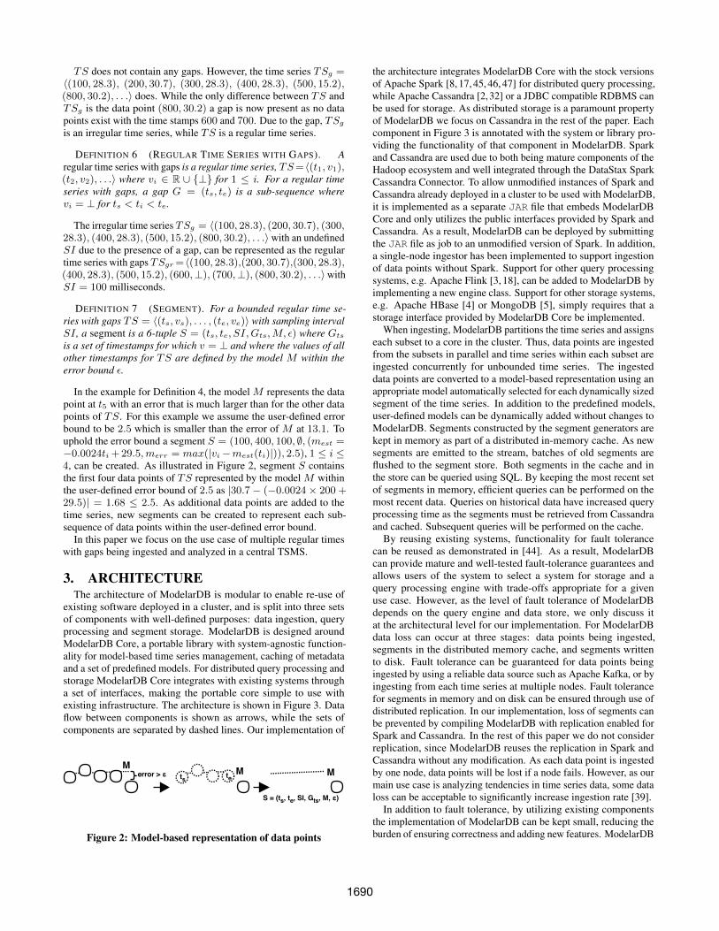
DEFINITION 7 (SEGMENT). For a bounded regular time se-ries with gaps TS = 〈(ts, vs), . . . , (te, ve)〉 with sampling intervalSI , a segment is a 6-tuple S = (ts, te, SI,Gts,M, ε) where Gts
is a set of timestamps for which v = ⊥ and where the values of allother timestamps for TS are defined by the model M within theerror bound ε.
In the example for Definition 4, the model M represents the datapoint at t5 with an error that is much larger than for the other datapoints of TS. For this example we assume the user-defined errorbound to be 2.5 which is smaller than the error of M at 13.1. Touphold the error bound a segment S = (100, 400, 100, ∅, (mest =−0.0024ti +29.5,merr = max(|vi−mest(ti)|)), 2.5), 1 ≤ i ≤4, can be created. As illustrated in Figure 2, segment S containsthe first four data points of TS represented by the model M withinthe user-defined error bound of 2.5 as |30.7− (−0.0024× 200 +29.5)| = 1.68 ≤ 2.5. As additional data points are added to thetime series, new segments can be created to represent each sub-sequence of data points within the user-defined error bound.
In this paper we focus on the use case of multiple regular timeswith gaps being ingested and analyzed in a central TSMS.
3. ARCHITECTUREThe architecture of ModelarDB is modular to enable re-use of
existing software deployed in a cluster, and is split into three setsof components with well-defined purposes: data ingestion, queryprocessing and segment storage. ModelarDB is designed aroundModelarDB Core, a portable library with system-agnostic function-ality for model-based time series management, caching of metadataand a set of predefined models. For distributed query processing andstorage ModelarDB Core integrates with existing systems througha set of interfaces, making the portable core simple to use withexisting infrastructure. The architecture is shown in Figure 3. Dataflow between components is shown as arrows, while the sets ofcomponents are separated by dashed lines. Our implementation of
M
S = (ts, te, SI, Gts, M, ε)
ts teMM
error > ε
Figure 2: Model-based representation of data points
the architecture integrates ModelarDB Core with the stock versionsof Apache Spark [8, 17, 45, 46, 47] for distributed query processing,while Apache Cassandra [2,32] or a JDBC compatible RDBMS canbe used for storage. As distributed storage is a paramount propertyof ModelarDB we focus on Cassandra in the rest of the paper. Eachcomponent in Figure 3 is annotated with the system or library pro-viding the functionality of that component in ModelarDB. Sparkand Cassandra are used due to both being mature components of theHadoop ecosystem and well integrated through the DataStax SparkCassandra Connector. To allow unmodified instances of Spark andCassandra already deployed in a cluster to be used with ModelarDB,it is implemented as a separate JAR file that embeds ModelarDBCore and only utilizes the public interfaces provided by Spark andCassandra. As a result, ModelarDB can be deployed by submittingthe JAR file as job to an unmodified version of Spark. In addition,a single-node ingestor has been implemented to support ingestionof data points without Spark. Support for other query processingsystems, e.g. Apache Flink [3, 18], can be added to ModelarDB byimplementing a new engine class. Support for other storage systems,e.g. Apache HBase [4] or MongoDB [5], simply requires that astorage interface provided by ModelarDB Core be implemented.
When ingesting, ModelarDB partitions the time series and assignseach subset to a core in the cluster. Thus, data points are ingestedfrom the subsets in parallel and time series within each subset areingested concurrently for unbounded time series. The ingesteddata points are converted to a model-based representation using anappropriate model automatically selected for each dynamically sizedsegment of the time series. In addition to the predefined models,user-defined models can be dynamically added without changes toModelarDB. Segments constructed by the segment generators arekept in memory as part of a distributed in-memory cache. As newsegments are emitted to the stream, batches of old segments areflushed to the segment store. Both segments in the cache and inthe store can be queried using SQL. By keeping the most recent setof segments in memory, efficient queries can be performed on themost recent data. Queries on historical data have increased queryprocessing time as the segments must be retrieved from Cassandraand cached. Subsequent queries will be performed on the cache.
By reusing existing systems, functionality for fault tolerancecan be reused as demonstrated in [44]. As a result, ModelarDBcan provide mature and well-tested fault-tolerance guarantees andallows users of the system to select a system for storage and aquery processing engine with trade-offs appropriate for a givenuse case. However, as the level of fault tolerance of ModelarDBdepends on the query engine and data store, we only discuss itat the architectural level for our implementation. For ModelarDBdata loss can occur at three stages: data points being ingested,segments in the distributed memory cache, and segments writtento disk. Fault tolerance can be guaranteed for data points beingingested by using a reliable data source such as Apache Kafka, or byingesting from each time series at multiple nodes. Fault tolerancefor segments in memory and on disk can be ensured through use ofdistributed replication. In our implementation, loss of segments canbe prevented by compiling ModelarDB with replication enabled forSpark and Cassandra. In the rest of this paper we do not considerreplication, since ModelarDB reuses the replication in Spark andCassandra without any modification. As each data point is ingestedby one node, data points will be lost if a node fails. However, as ourmain use case is analyzing tendencies in time series data, some dataloss can be acceptable to significantly increase ingestion rate [39].
In addition to fault tolerance, by utilizing existing componentsthe implementation of ModelarDB can be kept small, reducing theburden of ensuring correctness and adding new features. ModelarDB
1690

Figure 3: Architecture of a ModelarDB node, each contains query processing and storage to improve locality
is implemented in 1675 lines of Java code for ModelarDB Core and1429 lines of Scala code for the command-line and the interfaces toexisting systems. ModelarDB Core is implemented in Java to makeit simple to interface with the other JVM languages and to keepthe translation from source to bytecode as simple as possible whenoptimizing performance. Scala was used for the other componentsdue to increased productivity from pattern matching, type inference,and immutable data structures. The source code is available athttps://github.com/skejserjensen/ModelarDB.
4. DATA INGESTIONTo use the resources evenly, ingestion is performed in parallel
based on the number of threads available for that task and the sam-pling rate of the time series. The set of time series is partitioned intodisjoint subsets SS and assigned to the available threads so the datapoints per second of each subset are as close to equal as possible.Providing each thread with the same amount of data points to pro-cess, ensures resources are utilized uniformly across the cluster toprevent bottlenecks. The partitioning method used by ModelarDB isbased on [31], and minimizesmax(data points per minute(S1))−min(data points per minute(S2)) for S1, S2 ∈ SS.
4.1 Model-Agnostic Compression AlgorithmTo make it possible to extend the set of models provided by
ModelarDB Core, we propose an algorithm for segmenting andcompressing regular time series with gaps in which models usinglossy or lossless compression can be used. By optimizing the algo-rithm for regular time series with gaps as per our use case describedin Section 1, the timestamp of each data point can be discarded asthey can be reconstructed using the sampling interval stored for eachtime series and the start time end time stored as part of each seg-ment. To alleviate the trade-off between high compression and lowlatency required by existing multi-model compression algorithms,we introduce two segment types, namely a temporary segment (ST)
and a finalized segment (SF). The algorithm emits STs based ona user-defined maximum latency in terms of data points not yetemitted to the stream, while SFs are emitted when a new data pointcannot be represented by the set of models used. The general ideaof our algorithm is shown in Figure 4 and uses a list of models fromwhich one model is active at a time as proposed by [22]. For thisexample we set the maximum latency to be three data points, usea single model in the form of a linear function, and ingest the timeseries TS from Section 2. At t1 and t2, data points are added to atemporary buffer while a modelM is incrementally fitted to the datapoints. As our method is model-agnostic, each model defines how itis fitted to the data points and how the error is computed. This allowsmodels to implement the most appropriate method for fitting datapoints, e.g., models designed for streaming can fit one data point atime, while models that must be recomputed for each data point canperform chunking. At t3, three data points have yet to be emitted,see ye, and the model is emitted to the main memory segment cacheas a part of a ST. For illustration, we mark the last data point emittedas part of a ST with a T , and the last data points emitted as part of aSF with an F . As M might be able to represent more data points,the data points are kept in the buffer and the next data point is addedat t4. At t5, a data point is added which M cannot represent withinthe user-defined error bound. As our example only includes onemodel, a SF is emitted to the main memory segment cache and thedata points represented by the SF deleted from the buffer as shownby dotted circles, before the algorithm starts anew with the next datapoint. As the SF emitted represents the data point ingested at t4, yeis not incremented at t5 to not emit data points already representedby a SF as a part of a ST. Last, at tn, when the cache reaches auser-defined bulk write size, the segments are flushed to disk.
Our compression algorithm is shown in Algorithm 1. First vari-ables are initialized in Line 8-11, this corresponds to t0 in Figure 4.To ensure the data points can be reproduced from each segment, inLine 14-16, if a gap exists all data points in the buffer are emitted asone or more SFs. If the number of data points in the buffer is lower
Figure 4: The multi-model compression algorithm, maximum for yet to be emitted (ye) data points is three
1691

Algorithm 1 Online model-agnostic (lossy and lossless) multi-model compression algorithm with latency guarantees1: Let ts be the time series of data points.2: Let models be the list of models to select from.3: Let error be the user defined error bound.4: Let limit be the limit on the length of each segment.5: Let latency be the latency in not emitted data points.6: Let interval be the sampling interval of the time series.7:8: model ← head(models)9: buffer ← create list()
10: yet emitted ← 011: previous ← nil12: while has next(ts) do13: data point = retrieve next data point(ts)14: if time diff (previous, data point) > interval then15: flush buffer(buffer)16: end if17: append data point to buffer(data point , buffer)18: previous ← data point19: if append data point to model(
data point ,model , error , limit) then20: yet emitted ← yet emitted + 121: if yet emitted = latency then22: emit temporary segment(model , buffer)23: yet emitted ← 024: end if25: else if has next(models) then26: model ← next(models)27: initialize(model , buffer)28: else29: emit finalized segment(models, buffer)30: model ← head(models)31: initialize(model , buffer)32: yet emitted ← min(yet emitted , lengh(buffer))33: end if34: end while35: flush buffer(buffer)
than what is required to instantiate any of the provided models(a linear function requires two data points) a segment containinguncompressed values is emitted. In Line 17-20 the data point isappended to the buffer, and previous is set to the current data point.The data point is appended to model , allowing the model to updateits internal parameters and the algorithm to check if the model canrepresent the new data point within the user-defined error bound orlength limit. Afterwards, the number of data points not emitted as asegment is incremented. This incremental process is illustrated bystates t1 to t4 in Figure 4. If latency data points have not been emit-ted, a ST using the current model is emitted in Line 21-23. The cur-rent model is kept as it might represent additional data points. Thiscorresponds to t3 in Figure 4 as a ST is emitted due to latency = 3 .If the current model cannot be instantiated with the data points inthe buffer, a ST containing uncompressed values is emitted. Whenmodel no longer can represent a data point within the required errorbound, the next model in the list of models is selected and initializedwith the buffered data points in Line 25-27. As the model representsas many data points from buffer as possible when initialized, andany subsequent data points are rejected, no explicit check of if themodel can represent all data points in the buffer is needed. Instead,this check will be done as part of the algorithm’s next iteration whena new data point is appended. When the list of models becomes
empty, a SF containing the model with the highest compressionratio is emitted in Line 29. To allow for models using losslesscompression we compute the compression ratio as the reduction inbytes not the number of values to be stored: compression ratio =(data points represented(model) × size of (data point)) /size of (model). As model selection is based on the compressionratio, the segment emitted by emit finalized segment might notrepresent all data points in the buffer. In Line 30-32 model is set tothe first model in the list and initialized with any data points left inthe buffer. If data points not emitted by a ST were emitted as part ofthe SF, yet emitted is decremented appropriately. This process ofemitting a SF corresponds to t5 of Figure 4, where the latest datapoint is left in the buffer and one data point is emitted first by a SF.In Line 35 as all data points have been received, the buffer is flushedso all data points are emitted as SFs.
4.2 Considerations Regarding Data IngestionTwo methods exist for segmenting time series: connected and
disconnected. A connected segment starts with the previous seg-ment’s last data point, while a disconnected segment starts withthe first data point not represented by the previous segment. Ouralgorithm supports both by changing if emit finalized segmentkeeps the last data point of a segment when it is emitted. The use ofconnected segments provides two benefits. If used with models sup-porting interpolation, the time series can be reconstructed with anysampling interval as values between any two data points can be inter-polated. Also, connected segments can be stored using only a singletime stamp as the end time of one segment is the start time of thenext. However, for multi-model compression of time series [37, 38]demonstrated an increased compression ratio for disconnected seg-ments if the start and end time of each segment are stored for usewith indexing. The decreased size is due to the increased flexibil-ity when fitting disconnected segments as no data point from theprevious segment is included [37, 38]. Since time series may havegaps, the start and end time of a segment must be stored to ensureall data points ingested can be reconstructed. As a result, the rest ofthis paper will only be concerned with disconnected segments.
To represent gaps, there are two methods: flushing the stream ofdata points when a gap is encountered, or storing the gaps explicitlyas a pair of time stamps G = (ts, te). When we evaluated both weobserved no significant difference in compression ratio. However,storing gaps explicitly requires additional computation as any opera-tion on segments must skip gaps which also complicates the imple-mentation. Storing gaps explicitly requires flush buffer(buffer) inLine 15 in Algorithm 1 be substituted with timestamp(previous)and timestamp(data point) being added to a gap buffer and thatthe functions emitting segments are modified to include gaps as partof the segment. ModelarDB flushes the stream of data points asshown in Algorithm 1; but explicit storage of gaps can be enabled.
4.3 Implementation of User-Defined ModelsFor a user to optionally add a new model and segment in addition
to those predefined in ModelarDB Core, each must implement theinterfaces in Table 2. Tid is a unique id assigned to each time series.By having a segment class, a model object can store data whileingesting data points without increasing the size of its segment. Asa result, models can implement model-specific optimizations suchas chunking, lazy fitting or memoization. For aggregate queries tobe executed directly on a segment, the optional methods must beimplemented. An implementation of sum for a segment using alinear function as the model is shown in Listing 1. For this model,the sum can be computed without recreating the data points bymultiplying the average of the values with the number of represented
1692

Table 2: Interface for models and segments, is a required method and is an optional methodModelnew(Error, Limit) Return a new model with the user-defined error bound and length limit.append(Data Point) Append a data point if it and all previous do not exceed the error bound.initialize([Data Point]) Clear the existing data points from the model and append the data points from
the list until one exceeds the error bound or length limit.get(Tid, Start Time, End Time, SI, Parameters, Gaps) Create a segment represented by the model from serialized parameters.get(Tid, Start Time, End Time, SI, [Data Point], [Gap]) Create a segment from the models state and the list of data points.length() Return the number of data points the model currently represents.size() Return the size in bytes currently required for the models parameters.Segmentget(Timestamp, Index) Return the value from the underlying model that matches the timestamp and
index, both are provided to simplify implementation of this interface.parameters() Return the segment specific parameters necessary to reconstruct it.sum() Compute the sum of the values of data points represented by the segmentmin() Compute the minimum value of data points represented by the segment.max() Compute the maximum value of data points represented by the segment.
data points. In Line 2-3 the number of data points is computed. InLine 4-5 the minimum and maximum value of the segment. Last, inLine 6-7 the sum is computed by multiplying the average with thenumber of data points. As a result, the sum can be computed in tenarithmetic operations and without a loop.
1 public double sum() {2 int timespan = this.endTime - this.startTime;3 int size = (timespan / this.SI) + 1;4 double first = this.a * this.startTime + this.b;5 double last = this.a * this.endTime + this.b;6 double average = (first + last) / 2;7 return average * size;8 }
Listing 1: sum implemented for a linear model
To demonstrate we use the segment from Section 2 with the starttime 100, the end time 400, the sampling interval 100, and the linearfunction as−0.0024ti+29.5 as model. For a more realistic examplewe increase the end time to 7300. First the number of data pointsrepresented by the segment is calculated ((7300−100)/100)+1 =73, followed by the value of the first −0.0024 × 100 + 29.5 =29.26, and last data point −0.0024 × 7300 + 29.5 = 11.98. Theaverage value for the data points represented by the segment is then(29.26+11.98)/2 = 20.62, with the sum of the represented valuesgiven by 20.62 × 73 = 1505.26. Our example clearly shows thebenefit of using models for queries as computing the sum is reducedfrom 73 arithmetic operations to 10, or in terms of complexity, fromlinear to constant time complexity.
All models must exhibit the following behavior. A model yetto append enough data points to instantiate the model must returnan invalid compression ratio NaN so it is not selected to be part ofa segment. Second, if a model rejects a data point, all followingdata points must be rejected until the model is reinitialized. Last, asconsequence of using an extensible set of models, the method forcomputing the error of a model’s approximation must be defined bythe model. The combination of user-defined models and the modelselection algorithm provides a framework expressive enough to ex-press existing approaches for time series compression. For TSMSsthat compress time series as statically sized sub-sequences usingone compression method, such as Facebook’s Gorilla [39], a singlemodel which rejects data points based on the limit parameter can beused. For methods that use multiple lossy models in a predefinedsequence, such as [22], the same models can be implemented andre-used with any system that integrates ModelarDB Core, with the
added benefit that the ordering of the models are not hardcoded aspart of the algorithm as in [22] but simply a parameter.
For evaluation we implement a set of general-purpose modelsfrom the literature. We base our selection of models on [27] demon-strating substantial increases in compression ratio for models sup-porting dynamically sized segments and high compression ratiofor some constant and linear models, in addition to existing multi-model approaches predominately selecting constant and linear mod-els [22, 38]. Also we select models that can be fitted incrementallyto efficiently fit the data points online. To ensure the user-providederror bound is guaranteed for each data point, only models providingan error bound based on the uniform error norm are considered [34].Last, we select models with lossless and lossy compression, allowingModelarDB to select the approach most appropriate for each sub-sequence. We thus implement the following models: the constantPMC-MR model [33], the linear Swing model [23], both modifiedso the error bound can be expressed as the percentage differencebetween the real and approximated value, and the lossless compres-sion algorithm for floating-point values proposed by Facebook [39]modified to use floats. A model storing raw values is used byModelarDB when no other model is applicable.
5. QUERY PROCESSING
5.1 Generic Query InterfaceSegments emitted by the segment generators are put in the main-
memory cache and made available for querying together with seg-ments in storage. ModelarDB provides a unified query interface forsegments in memory and storage using two views. The first view rep-resents segments directly while the second view represents segmentsas data points. This segment view uses the schema (Tid int,StartTime timestamp,EndTime timestamp,SI int,Mid int, Parameters blob) and allows for aggregate que-ries to be executed on the segments without reconstructing thedata points. The attribute Tid is the unique time series id, SI thesampling interval, Mid the id of the model used for the segment,and Parameters the parameters for the model. The data pointview uses the schema (Tid int, TS timestamp, Valuefloat) to enable queries to be executed on data points recon-structed from the segments. Implementing views at these two levelsof abstraction allows query processing engines to directly inter-face with the data types utilized by ModelarDB Core. Efficientaggregates can be implemented as user-defined aggregate functions
1693

(UDAFs) on the segment view, and predicate push-down can be im-plemented to the degree that the query processing engine supports it.While only having the data point view would provide a simpler queryinterface, interfacing a new query processing engine with Mode-larDB Core would be more complex as aggregate queries to the datapoint view should be rewritten to use the segment view [21, 29, 43].
5.2 Query Interface in Apache SparkThrough Spark SQL ModelarDB provides SQL as its query lan-
guage. Since Spark SQL only pushes the required columns andthe predicates of the WHERE clause to the data source, aggregatesare implemented as UDAFs on the segment view. While full queryrewriting is not performed, the data point view retrieves segmentsthrough the segment view which pushes the predicates of the WHEREclause to the segment store. As a result, the segment store needsonly support predicate push-down from the segment view, and neverfrom both views. Our current implementation supports COUNT,MIN, MAX, SUM, and AVG. The UDAFs use the optional methodsfrom the segment interface shown in Table 2 if available, otherwisethe query is executed on data points. As UDAFs in Spark SQL can-not be overloaded, two sets of UDAFs are implemented. The first setoperate on segments as rows and have the suffix S. The second setoperate on segments as structs and have the suffix SS. Queries onsegments can be filtered at the segment level using a WHERE clause.Thus, for queries on the segment view to be executed with the samegranularity as queries on the data point view, functions are providedto restrict either the start time (START), end time (END), or both(INTERVAL) of segments. While ModelarDB at the moment onlysupports a limited number of built-in aggregate functions throughthe segment view, to demonstrate the benefit of computing aggre-gates using models, any aggregate functions provided as part ofSpark SQL can be utilized through the data point view. In addition,existing software developed to operate on time series as data points,e.g., for time series similarity search, can utilize the data point view.Last, using the APIs provided by Spark SQL any distributive oralgebraic aggregation function can be added to both the data pointview and the segment view.
5.3 Execution of Queries on ViewsExamples of queries on the views are shown in Listing 2. Line
1-2 show two queries calculating the sum of all values ingestedfor the time series with Tid = 3. The first computes the resultfrom data points reconstructed from the segments while the secondquery calculates the result directly from the segments. The query onLine 4-5 computes the averages of the values for data points with atimestamp after 2012-01-03 12:30. The WHERE clause filtersthe result at the segment level and START disregards the data thatis older than the timestamp provided. Last, in Line 7-8 a query isexecuted on the data point view as if the data points were stored.
1 SELECT SUM(Value) FROM DataPoint WHERE Tid = 32 SELECT SUM_S(*) FROM Segment WHERE Tid = 334 SELECT AVG_SS( START(*, '2012-01-03 12:30') )5 FROM Segment WHERE EndTime >= '2012-01-03 12:30'67 SELECT * FROM DataPoint WHERE Tid = 38 AND TS < '2012-04-22 12:25'
Listing 2: Query examples supported in ModelarDB
To lower query latency, the main memory segment cache, seeFigure 3, stores the most recently emitted or queried SFs and thelast ST emitted for each time series. Then, to ensure queries do notreturn duplicate data points, the start time of a ST is updated when aSF with the same Tid is emitted so the time intervals do not overlap.
Segment Store(Cassandra)
QueryProcessor
(Spark SQL)
TemporarySegments
(Spark)
FinalizedSegments
(Spark)
SegmentView
(Spark)
Data PointView
(Spark SQL)Client Queries
StorageSegments
(Spark)
Segment Stream
RS1 = { SF1, SF2, SF3 }
RS3 = { SF4, SF5 }
RS2 = { SF3 }
RS5 = { SF3, SF4, SF5, ST6 }
RS6 = { SF3, ST6 }
RS4 = { ST6 }
SELECT * FROM Segment WHERE Tid = 77 AND EndTime > '2012-01-03'
Figure 5: Query processing in ModelarDB
STs where StartTime > EndTime are dropped. Last, the SFcache is flushed when it reaches a user-defined bulk write size.
Query processing in ModelarDB is primarily concerned withfiltering out segments and data points from the query result. Anexample is shown in Figure 5 with a query for segments that containdata points from the sensor with Tid = 77 from after the date2012-01-03. Assume that only SF3 and ST6 satisfy both pred-icates and that SF3 is not in the cache. First, the WHERE clausepredicates are pushed to the segment store, see RS1, to retrieve therelevant segment. The segment retrieved from disk is cached, seeRS2, and the cache is then unioned with the STs and SFs in memory,shown as RS3 and RS4, to produce the set RS5. RS5 is filteredaccording to the WHERE clause to possibly remove segments pro-vided by a segment store with imprecise evaluation of the predicates(i.e., with false positives) and to remove irrelevant segments fromthe in-memory cache. The final result is shown as RS6. Queries onthe data point view are processed by retrieving relevant segmentsthrough the segment view. The data points are then reconstructedand filtered based on the WHERE clause.
5.4 Code-Generation for ProjectionsIn addition to predicate push-down, the views perform projections
such that only the columns used in the query are provided. However,building rows dynamically based on the columns requested creates asignificant performance overhead. As the columns of each view arestatic, optimized projection methods can be generated at compiletime without the additional overhead and complexity of dynamiccode generation.
1 def getDataPointGridFunction2 (columns: Array[String]): (DataPoint => Row) = {3 val target = getTarget(columns, dataPointView)4 (target: @switch) match {5 //Permutations of ('tid')6 case 1 => (dp: DataPoint) => Row(dp.tid)7 ...8 //Permutations of ('tid', 'ts', 'value')9 ...
10 case 321 => (dp: DataPoint) => Row(dp.value,11 new Timestamp(dp.timestamp), dp.tid)12 }13 }
Listing 3: Selection of method for a projection
The method generated for the data point view is shown in List-ing 3. On Line 3, the list of requested columns is converted tocolumn indexes and concatenated in the requested order to createa unique integer. This works for both views as each has less thanten columns and allows the projection method to be retrieved using
1694

a switch instead of comparing the contents of arrays. On Line 4,the projection method is retrieved using a match statement whichis compiled to an efficient lookupswitch [15].
6. SEGMENT STORAGEFigure 6 shows a generic schema for storing segments with the
metadata necessary for ModelarDB. It has three tables: TimeSeries for storing metadata about time series (the current im-plementation requires only the sampling interval), Model for stor-ing the model type contained in each segment, and last Segmentfor storing segments with the model parameters as blobs. Thebulk of the data is stored in the segment table. Compared toother work [22, 24, 38], the inclusion of both a Tid and the TimeSeries table allows queries for segments from different time se-ries with different sampling intervals to be served by one Segmenttable.
Tid (PK)1
3
...
EndTime1460442620000
1460645060000
...
Parameters0x3f50cfc0
0x3f1e ...
...
Mid (PK)1
2
3
NamePMC-MR
Swing
Tid (PK)1
2
3
SI60000
120000
30000
Mid1
2
...Time Series ModelSegment
StartTime (PK)1460442200000
1460642900000...
Figure 6: Generic schema for storage of segments
6.1 Segment Storage in Apache CassandraCompression is the primary focus for ModelarDB’s storage of
segments in Cassandra. As Cassandra expects each column in atable to be independent, using Tid, StartTime, EndTimeas the primary key only indicates to Cassandra that each partitionis fully sorted by StartTime. As a result, adding StartTimeand EndTime to the primary key does not allow direct lookup ofsegments. However, as segments are partitioned by Tid, insideeach partition the EndTime would be sorted as a consequence ofStartTime being sorted. We utilize this for ModelarDB by parti-tioning each table on their respective ids, and use EndTime as theclustering column for the segment table so segments are sorted as-cendingly by EndTime on disk. This allows the Size of a segmentto be stored instead of StartTime, for a higher compression ratio,while allowing ModelarDB to exploit the partitioning and orderingof the segment table when executing queries as Cassandra can filtersegments on EndTime while Spark loads segments until the re-quired StartTime is reached. The StartTime column cannotbe omitted due to the presence of gaps as explained in Section 4.2.To support indexing methods suitable for a specific storage systemlike in [24], secondary indexes can be implemented in ModelarDBas part of the storage interface shown in Figure 3.
6.2 Predicate Push-DownThe columns for which predicate push-down is supported in our
implementation are shown in Figure 7. Each cell in the table showshow a predicate on a specific column is rewritten before it is pushedto the segment view or storage. Cells for the column StartTimemarked with Spark takeWhile indicate that Spark reads rows fromCassandra in batches until the predicate represented by the cell isfalse for a segment. As explained above, this allows StartTimeto be replaced with the column Size which stores the number ofdata points in the segment. This reduces the storage needed for starttime without sacrificing its precision. When a segment is loaded,the start time of the segment can be recomputed as StartTime =EndTime - (Size * SI), allowing Spark to load segments
until the predicate represented by the cell is false for a segment. Non-equality queries on Tid are rewritten as Cassandra only supportsequality queries on a partitioning key.
7. EVALUATIONWe compare ModelarDB to the state-of-the-art big data systems
and file formats used in industry: Apache ORC [6,26] files stored inHDFS [42], Apache Parquet [7] files stored in HDFS, InfluxDB [13],and Apache Cassandra [32]. InfluxDB is running on a single node asthe open-source version does not support distribution. The numberof nodes used for each experiment is shown in the relevant figures.Multi-model compression for time series is also evaluated in [22,37,38]. We first present the cluster, data sets and queries used in theevaluation, then we describe each experiment.
7.1 Evaluation EnvironmentThe cluster consists of one master and six worker nodes con-
nected by 1 Gbit Ethernet. All nodes have an Intel Core i7-2620M2.70 GHz, 8 GiB of 1333 MHz DDR3 memory and a 7,200 RPMhard-drive. Each node runs Ubuntu 16.04 LTS, InfluxDB 1.4.2,InfluxDB-Python 2.12, Pandas 0.17.1, HDFS from Hadoop 2.8.0,Spark 2.1.0, Cassandra 3.9 and DataStax Spark Cassandra Connec-tor 2.0.2 on top of EXT4. The master is a Primary HDFS NameNode,Secondary HDFS NameNode and Spark Master. Each worker servesas an HDFS Datanode, a Spark Slave, and a Cassandra Node. Cas-sandra does not require a master node. Only the software necessaryfor an experiment is kept running and replication is disabled for allsystems. Disk space utilization is found with du. The time series arestored using the same schema as the Data Point View: Tid as a int,TS using each storage method’s native timestamp type, and Valueas a float. InfluxDB is an exception as it only supports double.Ingestion for all storage methods is performed using float. ForParquet and ORC, one file is created per time series using Spark andstored in HDFS with one folder created for each data set and fileformat pair, for InfluxDB time series are stored as one measurementwith the Tid as a tag, and for Cassandra we partition on Tid andorder each partition on TS and Value for the best compression.
The configuration of each system is, in general, left with its de-fault values. However, the memory available for Spark and eitherCassandra or HDFS, is statically allocated to prevent crashes. Todivide memory between query processing and data storage, we limitthe amount of memory Spark can allocate per node, so the restis available to Cassandra/HDFS and Ubuntu. Memory allocationis limited through Spark to ensure consistency across all experi-ments. The appropriate amount of memory for Spark is found byassigning half of the memory on each system to Spark and thenreduce the memory allocated for Spark until all experiments canrun successfully. We enable predicate push-down for Parquet andORC. The parameters used are shown in Table 3, with ModelarDB
Table 3: The parameters we use for the evaluationModelarDB ValueError Bound 0%, 1%, 5%, 10%Limit 50Latency 0Bulk Write Size 50,000
Spark Valuespark.driver.memory 4 GiBspark.executor.memory 3 GiBspark.streaming.unpersist falsespark.sql.orc.filterPushdown truespark.sql.parquet.filterPushdown true
Model Representation Type of CompressionPMC-MR [33] Constant Function Lossy CompressionSwing [23] Linear Function Lossy CompressionFacebook [39] Array of Delta Values Lossless CompressionUncompressed Values Array of Values No Compression
1695

Tid StartTime EndTime
Segment View Segment View
Tid StartTime EndTime
Casandra Segment StorageData Point View
Tid IN ? No Pushdown Tid IN ? StartTime IN ? EndTime IN ? Tid IN ? No Pushdown No Pushdown
Tid > ? EndTime > ?
Tid >= ? EndTime >= ?
Tid < ? StartTime < ?
StartTime <= ?Tid <= ?
Tid = ? StartTime <= ? ANDEndTime >= ?
Tid Timestamp
Tid IN ? Timestamp IN ?
Tid > ? Timestamp > ?
Tid >= ? Timestamp >= ?
Tid < ? Timestamp < ?
Timestamp <= ? Tid <= ?
Tid = ? Timestamp = ?
Tid Timestamp
Tid > ?
Tid >= ?
Tid < ?
Tid <= ?
Tid = ?
StartTime > ?
StartTime >= ?
StartTime < ?
StartTime <= ?
StartTime = ?
EndTime > ?
EndTime >= ?
EndTime < ?
EndTime <= ?
EndTime = ?
Tid IN (?+1..n)
Tid IN (?..n)
Tid IN (1..?-1)
Tid IN (1..?)
No Pushdown
No Pushdown
Spark takeWhile
Spark takeWhile
EndTime > ?
EndTime >= ?
EndTime < ?
EndTime <= ?
Tid = ? No Pushdown EndTime = ?
Figure 7: The two-step methods for predicate push-down utilized by ModelarDB
specific parameters in the upper left table, changes to Spark’s defaultparameters in the upper right table, and the models implementedin ModelarDB Core shown in the bottom table. The parametervalues are found to work well with the data sets and the hardwareconfiguration. The error bound is 10% when not stated explicitly.
7.2 Data Sets and QueriesThe data sets we use for the evaluation are regular time series
where gaps are uncommon. Each data set is stored as CSV files withone time series per file and one data point per line.
Energy Production High Frequency This data set is referredto as EH and consists of time series from energy production. Thedata was collected by us from an OPC Data Access server usinga Windows server connected to an energy producer. The data hasan approximate sampling interval of 100ms. As pre-processing weround the timestamps and remove data points with equivalent times-tamps due to rounding. This pre-processing step is only requireddue to limitations of our collection process and not present in aproduction setup. The data set is 582.68 GiB in size.
REDD The public Reference Energy Disaggregation Data Set(REDD) [30] is a data set of energy consumption from six housescollected over two months. We use the files containing energy usagein each house per second. Three of the twelve files have been sortedto correct a few out-of-order data points and the files from housesix removed due to irregular sampling intervals. As REDD fits intomemory on a single node, we extend it by replicating each file 2,500times by multiplying all values of each file with a random in therange [0.001, 1.001) and round each value to two decimals placesto ensure our results are not impacted by identical files. 2,500 isselected due to the amount of storage in our cluster. The data set is487.52 GiB in size, and is referred to as Extended REDD (ER). Weuse this public data set to enable reproducibility.
Energy Production This data set is referred to as EP and primar-ily consists of time series for energy production and is provided byan energy trading company. The data is collected over 508 days,has a sampling interval of 60s, and is 339 GiB in size. The data setalso contains entity specific measurements such as wind speed for awind turbine and horizontal irradiance for solar panels.
Queries The first set of queries (S-AGG) consists of small aggre-gate and GROUP BY queries and represents online analytics on oneor a few time series, e.g., correlated sensors, as analytical queriesare the intended ModelarDB use case. Both types of queries are re-stricted by Tid using a WHERE clause, with the GROUP BY queriesoperating on five time series each and GROUP on Tid. The secondset (L-AGG) consists of large aggregate and GROUP BY queries,which aggregate the entire data set and each GROUP BY queryGROUPs on Tid. L-AGG is designed to evaluate the scalability ofthe system when performing its intended use case. The third set(P/R) contains time point and range queries restricted by WHEREclauses with either TS or Tid and TS. P/R represents a user extract-ing a sub-sequence from a time series, which is not the intendedModelarDB use case, but included for completeness. We do notevaluate SQL JOIN queries as they are not commonly used withtime series, and similarity search is not yet built into ModelarDB.
7.3 ExperimentsIngestion Rate To remove the network as a possible bottleneck,
the ingestion rate is mainly evaluated locally on a worker node.For each system/format we ingest channel one from house oneof ER from gzipped CSV files (14.67 GiB) on local disks. Ex-cept for InfluxDB, ingestion is performed using a local instanceof Spark through spark-shell with its default parameters. As nomature Spark Connector to our knowledge exists for InfluxDB,we use the InfluxDB-Python client library [14]. The input filesare parsed using Pandas and InfluxDB-Python is configured witha batch size of 50,000. For Cassandra we increase the parame-ter batch size fail threshold in kb to 50 MiB to allowlarger batches. To determine ModelarDB’s scalability we also eval-uate its ingestion rate on the cluster in two different scenarios: BulkLoading (BL) without queries and Online Analytics (OA) with ag-gregate queries continuously executed on random time series usingthe Segment View. When using a single worker, ModelarDB usesthe single-node ingestor, and when it is distributed, Spark streamingwith one receiver per node, a micro-batch interval of five seconds,and latency set to zero so each data point is part of a segment onlyonce.
BL-1 BL-1 BL-1 BL-1 BL-1 BL-6 OA-6Scenarios
0
1
2
3
4
5
Millio
ns of
Dat
a Poin
ts pe
r Sec
ond
InfluxDBCassandraParquetORCModelarDB
0.04 0.090.67 0.61 0.44
2.37 2.36
Figure 8: Ingestion, ER
0% 0% 0% 0% 0% 1% 5% 10%Error Bound
0
25
50
75
100
125
Size
(GiB
)
InfluxDBCassandraParquetORCModelarDB
4.33
111.8
9
106.9
4
13.50
2.84
2.63
2.48
2.41
Figure 9: Storage, EH
0% 0% 0% 0% 0% 1% 5% 10%Error Bound
0
50
100
150
200
250
300
Size
(GiB
)
InfluxDBCassandraParquetORCModelarDB
80.48
223.1
323
6.70
71.48 83
.90
33.51
11.46
8.64
Figure 10: Storage, ER
0% 0% 0% 0% 0% 1% 5% 10%Error Bound
0
20
40
60
80
100
120
Size
(GiB
)
InfluxDBCassandraParquetORCModelarDB
19.61
101.8
2
92.36
19.97
18.21
17.61
14.89
12.27
Figure 11: Storage, EP
1696

0% 1% 5% 10%Error Bound
0
50
100
150M
odel
Use
d in
%PMC-MRSwing
97.63
0.00
2.37
98.17
0.15
1.68
98.51
0.35
1.13
98.66
0.47
0.88
Figure 12: Models, EH
0% 1% 5% 10%Error Bound
0
50
100
150
Mod
el U
sed
in %
PMC-MRSwing
1.12
> 0
98.88
62.12
4.8133
.07
79.95
2.2017
.85
82.86
1.0516
.09
Figure 13: Models, ER
0% 1% 5% 10%Error Bound
0
50
100
150
Mod
el U
sed
in %
PMC-MRSwing
7.93
0.01
92.06
12.64
2.88
84.49
22.60
13.01
64.39
28.82
20.69
50.49
Figure 14: Models, EP
1000 500 250 100 50 25Average Distance Between Outliers
2
4
6
8
Relat
ive In
crea
se to
no
Outli
ers
EH - Error 0%EH - Error 10%ER - Error 0%ER - Error 10%EP - Error 0%EP - Error 10%
Figure 15: Outlier Effect
The results are shown in Figure 8. As expected InfluxDB andCassandra had the lowest ingestion rate, as they are designed tobe queried while ingesting. ModelarDB also supports executingqueries during ingestion but still provides 11 times and 4.89 timesfaster ingestion than InfluxDB and Cassandra, respectively. Par-quet and ORC provided 1.52 and 1.39 times increase compared toModelarDB, respectively. However, an entire file must be writtenbefore Parquet and ORC can be queried, making them unsuitablefor online analytics due to the inherent latency of this approach.This compromise is not needed for ModelarDB as queries can beexecuted on data as it is ingested. When bulk loading on the sixnode cluster the ingestion rate for ModelarDB increases 5.39 times,a close to linear speedup. The ingestion is nearly unaffected, a 5.36times increase, when doing online analytics in parallel. In summary,ModelarDB, achieves high ingestion rates while allowing onlineanalytics, unlike the alternatives.
Effect of Error Bound and Outliers The trade-off between stor-age efficiency and error bound is evaluated using all three data sets.The models used and size of each data set are found when storedin ModelarDB with the error bound set to values from 0% to 10%.We compare the storage efficiency of ModelarDB with the systemsused in industry. In addition, we evaluate the performance of Mod-elarDB’s adaptive compression method when outliers are present,by adding an increasing number of outliers to each data set. Theoutliers are randomly created such that the average distance betweentwo consecutive outliers is N and the value of each outlier is set to(Value of Data Point to Replace + 1) ∗ 2.
The storage used for EH is seen in Figure 9. Of the existingsystems, InfluxDB performs the best, but even with a 0% errorbound, ModelarDB reduces the size of EH 1.52 times compared toInfluxDB. This is expected as the PMC-MR model can be used toperform run-length encoding while changing values are managedwith delta-compression using the Facebook model. Increasing theerror bound to 10% provides a further 1.18 times reduction, whilethe average actual error is only 0.005%. The results for ER are seenin Figure 10. Compared to InfluxDB, ModelarDB provides muchbetter compression: 2.40 times for 1%, 7.02 times for 5%, and 9.31times 10% error bound. For ER, ORC is best of the existing systems,but ModelarDB further reduces by 2.13 times for 1%, 6.24 times for
5%, and 8.27 times for 10% error bound. In addition, average actualerror for ER is only 0.22% with 1% bound, 1.25% for 5% boundand 2.50% for 10% bound. Even with a 0% bound, ModelarDBuses just 1.17 times more storage than ORC. EP results are shownin Figure 11. Here, ModelarDB provides the best compression, evenat 0% error bound, however, the difference is smaller than for EHand ER. This is expected, as the EH and ER sampling intervalsare 600 and 60 times lower, respectively, yielding more data pointswith similar values due to close time proximity. ModelarDB alsomanages to keep the average actual error for EP low at only 0.08%for 1%, 0.48% for 5% and 0.73% for a 10% bound.
The models utilized for each data set are shown in Figure 12—14.Overall PMC-MR and Facebook are the most utilized models, withSwing used sparingly except for EP with 5% and 10% error. Note,that Swing also is utilized for ER and EP with a 0% error boundas perfectly linear increases and decreases of values do exist in thedata sets. Last, except for EH, multiple models are used extensively.These results clearly show the benefit and adaptivity of multi-modelcompression as each combination of data set and error bound canbe handled efficiently using different combinations of the models.
The effect of outliers is shown in Figure 15. As expected thestorage used increases with the number of outliers, but the increasedepends on the data set and error bound. For all data sets, Mode-larDB degrades gracefully as additional outliers are added to thedata set. As the values of N decrease below 250 the relative sizeincreases more rapidly as the high number of outliers severely re-strict the length of the segments ModelarDB can construct. Theresults also show that ModelarDB is more robust against outlierswhen a 0% error bound is used. With a 10% error bound the relativeincrease for EH and EP is slightly higher than for a 0% error bound,while the relative size increase for ER with a 10% error bound inthe extreme case of N = 25 is 9.06 while it is only 1.12 with a 0%error bound. This is expected as ER has a high compression ratiowith a 10% error bound and the high number of outliers preventsModelarDB from constructing long segments. The results show thatalthough designed for time series with few outliers, ModelarDBdegrades gracefully as the amount of outliers increases.
In summary, ModelarDB provides as good compression as theexisting formats when a 0% error bound is used, and much better
CLI-1 SV-1 DPV-1 DF-6 DF-6 DF-6 SV-6 DPV-6Utilized Query Interface
0
20
40
60
80
Runt
ime
(H)
InfluxDBModelarDBCasssandraParquetORC41.41
14.05
31.91
78.84
4.134.532.715.86
Figure 16: L-AGG, ER
1 2 4 8 16 32Number of Nodes
1
2
4
8
16
32
Rela
tive
Incr
ease
Segment ViewData Point View
Figure 17: Scale-out
L-Agg (SV) L-Agg (DPV) P/R (DPV)Query Type Performed
0.0
2.5
5.0
7.5
10.0
12.5
15.0
Runt
ime
(H)
NoneStatic
Dynamic
2.97
2.71 3.0
3
9.40
5.86 6.7
7
0.35
0.36
0.41
Figure 18: Projection, ER
L-Agg (SV) L-Agg (DPV) P/R (DPV)Query Type Performed
0.0
2.5
5.0
7.5
10.0
12.5
15.0
Runt
ime
(H)
NoneTid
Tid, TimestampTid, TimestampTakeWhile
2.762.8
42.9
62.7
1
6.186.3
56.3
35.8
6
2.53
0.620.4
50.3
6
Figure 19: Predicate, ER
1697

1000
1500
2000InfluxDBCassandraParquetORCModelarDB
CLI-1 DF-6 DF-6 DF-6 SV-6 DPV-6Utilized Query Interface
0
20
40
Runt
ime
(M)
17.93
1520.12
4.0013.92 9.96
30.56
Figure 20: S-AGG, EH
CLI-1 DF-6 DF-6 DF-6 SV-6 DPV-6Utilized Query Interface
0
50
100
150
200
Runt
ime
(M)
InfluxDBCassandraParquetORCModelarDB
0.5423.16
191.64
30.81
0.67 1.19
Figure 21: S-AGG, ER
CLI-1 DF-6 DF-6 DF-6 SV-6 DPV-6Utilized Query Interface
0
20
40
60
80
100
120
Runt
ime
(M)
InfluxDBCassandraParquet
ORCModelarDB
0.35 6.12
70.99
37.71
0.54 0.77
Figure 22: S-AGG, EP
CLI-1 DF-6 DF-6 DF-6 DPV-6Utilized Query Interface
0
20
40
60
80
Runt
ime
(M)
InfluxDBCassandraParquet
ORCModelarDB
0.3310.49
45.27
0.79
26.54
Figure 23: P/R, EH
compression for even a small error bound, by combining differentmodels depending on the data and error bound.
Scale-out To evaluate ModelarDB’s scalability we first compareit to the existing systems when executing L-AGG on ER using thetest cluster. Then, to determine the scalability of ModelarDB onlarge clusters, we execute L-AGG on Microsoft Azure using 1—32Standard D8 v3, the node type is selected based on the documenta-tion for Spark, Casandra and Azure [1,9,10]. The configuration fromthe test cluster is used with the exception that Spark and Cassandraeach have access to 50% of each node’s memory as no crashes wereobserved with this initial configuration. For each experiment REDDis duplicated, using the method described above, and ingested soeach node stores compressed data equivalent to the node’s memory.This makes caching the data set in memory impossible for Sparkand Cassandra. The number of nodes and data size are scaled inparallel based on existing evaluation methodology for distributedsystems [19]. Queries are executed using the most appropriatemethod for each system: InfluxDB’s command-line interface (CLI),ModelarDB’s Segment View (SV) and Data Point View (DPV), andfor Cassandra, Parquet, and ORC a Spark SQL Data Frame (DF).We evaluate the query performance using a DF and a cached DataFrame (DFC) as shown in Figure 25. However, as DFCs increasedthe run-time, as the data was inefficiently spilled to disk, we onlyuse DFs for the other queries.
The results are shown in Figure 16—17. For both views Mode-larDB achieves close to linear scale-up. This is expected as queriescan be answered with no shuffle operations as all segments of a timeseries are co-located. However, using SV, the query processing timeis significantly reduced as SV does not reconstruct the data pointswhich reduces both CPU and memory usage. On one node SV is2.27 times faster than DPV, and 2.16 times faster with six nodes. ForL-AGG on ER, ModelarDB is faster than all the existing systems.Compared to InfluxDB, on one node, ModelarDB is 2.95 times and1.30 times faster for SV and DPV, respectively. Using six nodes,ModelarDB is 1.52 times and 1.67 times faster than Parquet andORC, respectively. In summary, ModelarDB scales almost linearlywhile providing better performance than the competitors.
Effect of Optimizations To evaluate the code generation andpredicate push-down optimizations, we execute L-AGG and P/Ron ER both with and without the optimizations. As a comparisonto static code generation, we implement a straightforward dynamiccode generator using scala.tools.reflect.ToolBox andSpark’s mapPartitions transformation. By default ModelarDBuses static code-generation for projections and predicate push-downfor Tid, Timestamp, and takeWhile. The results for projec-tion in Figure 18 show that generating optimized code for projectionsdecreases the run-time up to 1.60 times compared to constructingeach row dynamically. However, using our implementation of dy-namic code generation increases the run-time compared to our staticcode generation. The results for predicate push-down are seen inFigure 19. Predicate push-down has little effect on the query pro-
cessing time for L-AGG, but the reduction is more pronounced forP/R where we see a 7.03 times reduction. This is to be expected asall queries in L-AGG must read the entire data set from disk, whileall queries in P/R can be answered using only a small subset.
Further Query Processing Performance To further evaluate thequery performance of ModelarDB, we execute S-AGG and P/R onall data sets using the query interfaces described for scale-out.
The results for S-AGG are shown in Figures 20—22. Once againthe run-time is reduced using the SV. While InfluxDB performsslightly better than ModelarDB for S-AGG on ER and EP, it islimited in terms of scalability and ingestion rate, as shown abovewhere ModelarDB executes L-AGG on ER 2.95 times faster thanInfluxDB. Compared to the distributed systems, ModelarDB pro-vides as good, or better query processing times for nearly all cases.On EH, ModelarDB is 1.4 times faster than ORC and 152.62 timesfaster than Cassandra. For EH, Parquet is faster, but for all otherdata sets ModelarDB is faster and uses much less storage space.For ER, which is a core use case scenario, ModelarDB reduces thequery processing time by staggering 34.57, 286.03 and 45.99 times,compared to Cassandra, Parquet and ORC, respectively. Last, forEP, Cassandra and ModelarDB provide the lowest query process-ing time with ModelarDB being 11.33 times faster. Thus for ourexperiments ModelarDB improves the query processing time sig-nificantly compared to the other distributed systems, in core casesby large factors, while it for small-scale aggregate queries remainscompetitive with an optimized single node system.
The results for P/R are shown in Figures 23—25. For P/R, In-fluxDB and Cassandra perform the best, which contrasts our scale-out experiment where they perform the worst. Clearly these systemsare optimized for queries on a small subset of a data set, while Par-quet, ORC, and ModelarDB, are optimized for aggregates on largedata sets. While P/R queries are not a core use case, ModelarDBprovides equivalent performance for P/R queries in most cases andis only significantly slower for EH. When compared to ORC andParquet, ModelarDB is in general faster and in the best case, ER,provides 1.63 times faster query processing time. In one singleinstance, for EH, ORC is 33.59 times faster than ModelarDB due tobetter predicate push-down, as disabling predicate push-down forORC increases the run-time from 47.64 seconds to 1 hour and 40
CLI-1 DF-6 DF-6 DF-6 DPV-6Utilized Query Interface
0
50
100
150
200
250
300
Runt
ime
(M)
InfluxDBCassandraParquet
ORCModelarDB
18.55 6.43
137.84
34.89 21.43
Figure 24: P/R, ER
CLI-1 DF-6 DFC-6 DF-6 DFC-6 DF-6 DFC-6DPV-6Utilized Query Interface
0
100
200
300
400
500
Runt
ime
(M)
InfluxDBCassandraParquet
ORCModelarDB
2.495.88
266.78
69.20
214.18
8.55
185.09
8.64
Figure 25: P/R, EP
1698

minutes. However, unlike Parquet and ORC, time series ingestedby ModelarDB can be queried online. An interesting result was thatDFCs increased the query processing time, particularly for the firstquery. This indicates that the data set is read from and spilled to diskdue to a lack of memory during the initial query with subsequentqueries executed using Spark’s on-disk format.
For our experiments, the other systems require a trade-off asthey are either good at large aggregate queries or point/range andsmall aggregate queries and support online analytics, but not both.ModelarDB hits a sweet spot, improving the state-of-the-art foronline analytics by providing fast ingestion, better compression andscalability for large aggregate queries while remaining competitivewith other systems for small aggregate and point-range queries. Thiscombination of features is not provided by any competitor.
8. RELATED WORKManagement of sensor data using models has received much
attention as the amounts of data have increased. We provide adiscussion of the most relevant related methods and systems. For asurvey of model-based sensor data management see [41], while asurvey of TSMSs can be found in [28].
Methods have been proposed for online construction of approx-imations with minimal error [25], or maximal segment length forbetter compression [34]. As the optimal model can change over time,methods using multiple mathematical models have been developed.In [37] each data point in the time series is approximated by allmodels in a set. A model is removed from the set if it cannot repre-sent a data point within the error bound. When the set of models isempty, the model with the highest compression ratio is stored andthe process restarted. A relational schema for segments was dis-cussed in [38]. The Adaptive Approximation (AA) algorithm [40]uses functions as models with an extensible method for computingthe coefficients. The AA algorithm approximates each data pointin the time series until a model exceeds the error bound and a localsegment is created for that model and the model reset. After allmodels have constructed one local segment, the segments using thelowest number of parameters are stored. An algorithm based onregression was proposed in [22]. It approximates data points with asingle polynomial model and then increases the number of coeffi-cients as the error bound becomes unsatisfiable. As the user-definedmaximum number of coefficients is reached, the model with thehighest compression ratio is stored and the time series rewound tothe last data point of the stored segment. In this paper, we propose amulti-model compression algorithm for time series that improves onthe state-of-the-art as it supports user-defined models, supports lossyand lossless models, and removes the trade-off between compressionand latency inherent to the existing methods.
In addition to techniques for representing time series as mod-els, RDBMSs with support for models have also been proposed.MauveDB [21] supports using models for data cleaning withoutexporting the data to another application. Models are explicitlyconstructed from a table with raw data and then maintained by theRDBMS. Model-based views created with a static sampling inter-val serve as the query interface for the models. FunctionDB [43]natively supports polynomial functions as models. The RDBMS’squery processor evaluates queries directly on these models whenpossible, with the query results provided as discrete values. Modelfitting is performed manually by fitting a specific model to a table.Maintenance of the constructed models is outside the scope of the pa-per. Plato [29] allows for user-defined models. Queries are executedon models if the necessary functions are implemented and discretevalues if not. The granularity at which to instantiate a model for aquery can be specified with a grid operator or left to Plato. Fitting
models to a data set is done manually as automated model selectionis left as future work. Tristan [36], based on the MiSTRAL architec-ture [35], approximates time series as sequences of fixed-length timeseries patterns using dictionary compression. Before ingestion a dic-tionary must be trained offline on historical data. During ingestion afixed number of data points are buffered before the compression isapplied and the dictionary updated with new patterns if necessary.For approximate query processing a subset of the patterns stored fora time series is used. A distributed approach to model-based storageof time series using an in-memory tree-based index, a key-valuestore, and MapReduce [20] was proposed by [24]. The segmentationis performed using Piecewise Constant Approximation (PCA) [41].Each segment is stored and indexed twice, once by time and once byvalue. Query processing is performed by locating segments usingthe index, retrieving segments from the store using mappers, andlast, instantiating each model using reducers. ModelarDB hits asweet spot and provides functionality in a single extensible TSMSnot present in the existing systems: storage and query processing fortime series within a user-defined error bound [21, 29, 43], supportfor both fixed and dynamically sized user-defined models that canbe fitted online without requiring offline training of any kind [36],and automated selection of the most appropriate model for each partof a time series while also storing each segment only once [24].
9. CONCLUSION & FUTURE WORKMotivated by the need for storage and analysis of big amounts of
data from reliable sensors, we presented a general architecture for amodular model-based TSMS and a concrete system using it, Mode-larDB. We proposed a model-agnostic extensible and adaptive multi-model compression algorithm that supports both lossless and lossycompression within a user-defined error bound. We also presentedgeneral methods and optimizations usable in a model-based TSMS:(i) a database schema for storing multiple distinct time series as (pos-sibly user-defined) models, (ii) methods to push-down predicates toa key-value store that utilizes the presented schema, (iii) methods toexecute optimized aggregate functions directly on models withoutrequiring a dynamic optimizer, (iv) static code-generation to opti-mize execution of projections, (v) dynamic extensibility that allowsuser-defined models to be added and used without recompiling theTSMS. The architecture was realized as a portable library whichwas interfaced with Apache Spark for query processing and ApacheCassandra for storage. Our evaluation showed that, unlike currentsystems, ModelarDB hits a sweet spot and achieves fast ingestion,good compression, almost linear scale-out, and fast aggregate queryprocessing, in the same system, while also supporting online queries.The evaluation further demonstrated how the contributions effec-tively work together to adapt to the data set using multiple models,that the actual errors are much lower than the bounds, and howModelarDB degrades gracefully as outliers are added.
In future work we are planning to extend ModelarDB in multipledirections: (i) Increase query performance by developing new tech-niques for indexing segments represented by user-defined models,performing similarity search directly on user-defined models, andperforming dynamic optimizations utilizing that the time series arerepresented as models. (ii) Reduce the storage needed for largevolumes of sensor data by representing correlated streams of sensordata as a single stream of segments. (iii) Further simplify use ofModelarDB by removing or automatically inferring parameters.
10. ACKNOWLEDGEMENTSThis research was supported by the DiCyPS center funded by In-
novation Fund Denmark [12], and Microsoft Azure for Research [16].
1699

11. REFERENCES[1] Apache Cassanddra - Hardware Choices.
http://cassandra.apache.org/doc/latest/operating/hardware.html. Viewed: 2018-07-15.
[2] Apache Cassandra.http://cassandra.apache.org/. Viewed:2018-07-15.
[3] Apache Flink. https://flink.apache.org/. Viewed:2018-07-15.
[4] Apache HBase. https://hbase.apache.org/.Viewed: 2018-07-15.
[5] Apache MongoDB. https://www.mongodb.com/.Viewed: 2018-07-15.
[6] Apache ORC. https://orc.apache.org/. Viewed:2018-07-15.
[7] Apache Parquet. https://parquet.apache.org/.Viewed: 2018-07-15.
[8] Apache Spark. https://spark.apache.org/.Viewed: 2018-07-15.
[9] Apache Spark - Hardware Provisioning.https://spark.apache.org/docs/2.1.0/hardware-provisioning.html. Viewed: 2018-07-15.
[10] Azure Databricks.https://azure.microsoft.com/en-us/pricing/details/databricks/. Viewed:2018-07-15.
[11] DB-Engines Ranking.https://db-engines.com/en/ranking. Viewed:2018-07-15.
[12] DiCyPS - Center for Data-Intensive Cyber-Physical Systems.http://www.dicyps.dk/dicyps-in-english/.Viewed: 2018-07-15.
[13] InfluxData InfluxDB.https://www.influxdata.com/. Viewed:2018-07-15.
[14] InfluxDB API Client Libraries.https://docs.influxdata.com/influxdb/v1.4/tools/api_client_libraries/. Viewed:2018-07-15.
[15] Java Virtual Machine Specification.https://docs.oracle.com/javase/specs/jvms/se8/html/jvms-3.html#jvms-3.10.Viewed: 2018-07-15.
[16] Microsoft Azure for Research.https://www.microsoft.com/en-us/research/academic-program/microsoft-azure-for-research/. Viewed: 2018-07-15.
[17] M. Armbrust, R. S. Xin, C. Lian, Y. Huai, D. Liu, J. K.Bradley, X. Meng, T. Kaftan, M. J. Franklin, A. Ghodsi, andM. Zaharia. Spark SQL: Relational Data Processing in Spark.In Proceedings of SIGMOD, pages 1383–1394. ACM, 2015.
[18] P. Carbone, A. Katsifodimos, S. Ewen, V. Markl, S. Haridi,and K. Tzoumas. Apache Flink: Stream and Batch Processingin a Single Engine. Bulletin of the IEEE Computer SocietyTechnical Committee on Data Engineering, 38(4):28–38,2015.
[19] B. F. Cooper, A. Silberstein, E. Tam, R. Ramakrishnan, andR. Sears. Benchmarking Cloud Serving Systems with YCSB.In Proceedings of SOCC, pages 143–154. ACM, 2010.
[20] J. Dean and S. Ghemawat. MapReduce: Simplified DataProcessing on Large Clusters. In Proceedings of OSDI, pages137–150. USENIX, 2004.
[21] A. Deshpande and S. Madden. MauveDB: SupportingModel-based User Views in Database Systems. InProceedings of SIGMOD, pages 73–84. ACM, 2006.
[22] F. Eichinger, P. Efros, S. Karnouskos, and K. Bohm. Atime-series compression technique and its application to thesmart grid. The VLDB Journal, 24(2):193–218, 2015.
[23] H. Elmeleegy, A. K. Elmagarmid, E. Cecchet, W. G. Aref, andW. Zwaenepoel. Online piece-wise linear approximation ofnumerical streams with precision guarantees. PVLDB,2(1):145–156, 2009.
[24] T. Guo, T. G. Papaioannou, and K. Aberer. Efficient Indexingand Query Processing of Model-View Sensor Data in theCloud. Big Data Research, 1:52–65, 2014.
[25] T. Guo, Z. Yan, and K. Aberer. An Adaptive Approach forOnline Segmentation of Multi-Dimensional Mobile Data. InProceedings of MobiDE, pages 7–14. ACM, 2012.
[26] Y. Huai, A. Chauhan, A. Gates, G. Hagleitner, E. N. Hanson,O. O’Malley, J. Pandey, Y. Yuan, R. Lee, and X. Zhang. MajorTechnical Advancements in Apache Hive. In Proceedings ofSIGMOD, pages 1235–1246. ACM, 2014.
[27] N. Q. V. Hung, H. Jeung, and K. Aberer. An Evaluation ofModel-Based Approaches to Sensor Data Compression. IEEETKDE, 25(11):2434–2447, 2013.
[28] S. K. Jensen, T. B. Pedersen, and C. Thomsen. Time SeriesManagement Systems: A Survey. IEEE TKDE,29(11):2581–2600, 2017.
[29] Y. Katsis, Y. Freund, and Y. Papakonstantinou. CombiningDatabases and Signal Processing in Plato. In Proceedings ofCIDR, 2015.
[30] J. Z. Kolter and M. J. Johnson. REDD: A Public Data Set forEnergy Disaggregation Research. In Proceedings of SustKDD,2011.
[31] R. E. Korf. Multi-Way Number Partitioning. In Proceedingsof IJCAI, pages 538–543, 2009.
[32] A. Lakshman and P. Malik. Cassandra: A DecentralizedStructured Storage System. ACM SIGOPS Operating SystemsReview, 44(2):35–40, 2010.
[33] I. Lazaridis and S. Mehrotra. Capturing Sensor-GeneratedTime Series with Quality Guarantees. In Proceedings of ICDE,pages 429–440. IEEE, 2003.
[34] G. Luo, K. Yi, S.-W. Cheng, Z. Li, W. Fan, C. He, and Y. Mu.Piecewise Linear Approximation of Streaming Time SeriesData with Max-error Guarantees. In Proceedings of ICDE,pages 173–184. IEEE, 2015.
[35] A. Marascu, P. Pompey, E. Bouillet, O. Verscheure, M. Wurst,M. Grund, and P. Cudre-Mauroux. MiSTRAL: AnArchitecture for Low-Latency Analytics on Massive TimeSeries. In Proceedings of Big Data, pages 15–21. IEEE, 2013.
[36] A. Marascu, P. Pompey, E. Bouillet, M. Wurst, O. Verscheure,M. Grund, and P. Cudre-Mauroux. TRISTAN: Real-TimeAnalytics on Massive Time Series Using Sparse DictionaryCompression. In Proceedings of Big Data, pages 291–300.IEEE, 2014.
[37] T. G. Papaioannou, M. Riahi, and K. Aberer. Towards OnlineMulti-Model Approximation of Time Series. In Proceedingsof MDM, volume 1, pages 33–38. IEEE, 2011.
[38] T. G. Papaioannou, M. Riahi, and K. Aberer. Towards OnlineMulti-Model Approximation of Time Series. Technical report,EPFL LSIR, 2011.
[39] T. Pelkonen, S. Franklin, J. Teller, P. Cavallaro, Q. Huang,J. Meza, and K. Veeraraghavan. Gorilla: A Fast, Scalable,
1700

In-Memory Time Series Database. PVLDB, 8(12):1816–1827,2015.
[40] J. Qi, R. Zhang, K. Ramamohanarao, H. Wang, Z. Wen, andD. Wu. Indexable online time series segmentation with errorbound guarantee. World Wide Web, 18(2):359–401, 2015.
[41] S. Sathe, T. G. Papaioannou, H. Jeung, and K. Aberer. ASurvey of Model-based Sensor Data Acquisition andManagement. In Managing and Mining Sensor Data, pages9–50. Springer, 2013.
[42] K. Shvachko, H. Kuang, S. Radia, and R. Chansler. TheHadoop Distributed File System. In Proceedings of MSST,pages 1–10. IEEE, 2010.
[43] A. Thiagarajan and S. Madden. Querying ContinuousFunctions in a Database System. In Proceedings of SIGMOD,pages 791–804. ACM, 2008.
[44] D. Xie, F. Li, B. Yao, G. Li, L. Zhou, and M. Guo. Simba:Efficient In-Memory Spatial Analytics. In Proceedings ofSIGMOD, pages 1071–1085. ACM, 2016.
[45] M. Zaharia, M. Chowdhury, M. J. Franklin, S. Shenker, andI. Stoica. Spark: Cluster Computing with Working Sets. InProceedings of HotCloud. USENIX, 2010.
[46] M. Zaharia, T. Das, H. Li, T. Hunter, S. Shenker, and I. Stoica.Discretized Streams: Fault-Tolerant Streaming Computationat Scale. In Proceedings of SIGOPS, pages 423–438. ACM,2013.
[47] M. Zaharia, T. Das, H. Li, S. Shenker, and I. Stoica.Discretized Streams: An Efficient and Fault-Tolerant Modelfor Stream Processing on Large Clusters. In Proceedings ofHotCloud. USENIX, 2012.
1701