model uncertainty and exchange rate volatility

INTERNATIONAL ECONOMIC REVIEWVol. 53, No. 3, August 2012

MODEL UNCERTAINTY AND EXCHANGE RATE VOLATILITY∗

BY AGNIESZKA MARKIEWICZ1

Erasmus University Rotterdam, the Netherlands

This article proposes an explanation for shifts in the volatility of exchange-rate returns. Agents are uncertain aboutthe true data generating model and deal with this uncertainty by making inference on the models and their parameters’approach, I call model learning. Model learning may lead agents to focus excessively on a subset of fundamentalvariables. Consequently, exchange-rate volatility is determined by the dynamics of these fundamentals and changes asagents alter models. I investigate the empirical relevance of model learning and find that the change in volatility ofGBP/USD in 1993 was triggered by a shift between models.

1. INTRODUCTION

A well known and much documented fact in international economics is the presence ofshifts in the volatility of exchange rates. Floating exchange rates display low and high volatilityregimes, as documented by Engel and Hamilton (1990). Numerous researchers attempted tolink these volatility shifts to the dynamics of macroeconomic fundamental variables. Mussa(1986), Gerlach (1988), Baxter and Stockman (1989), and Flood and Rose (1995) observed thatin low inflation countries, the variability of most of the aggregate variables is unaffected by theexchange-rate regime. As a result, the consensus emerged that there is remarkably little evidenceof a systematic relationship between the volatilities of exchange rates and macroeconomicvariables. Yet, this consensus is inconsistent with theories that model the exchange rate as avariable reflecting underlying economic shocks.

The empirical literature suggests that parameter instability is an explanation for the difficultiesin finding a link between the macroeconomic variables and exchange rates. Schinasi and Swamy(1989) show that time-varying parameter exchange-rate models outperform the random walkin out-of-sample forecasting. Cheung et al. (2005), Rossi (2006), and Sarno and Valente (2009)find that the predictive power of different fundamental exchange-rate models depends on theparticular currency and the forecast horizon considered.

This article proposes a theoretical framework that can explain a time-varying link betweenexchange rates and the underlying fundamental macroeconomic variables. This is demonstratedusing a standard present value exchange-rate model in which agents are uncertain about thetrue model and its corresponding parameters. They deal with this model uncertainty by makinginferences about the models and their parameters. This mechanism will be called “modellearning.” The article demonstrates that learning about the exchange-rate model may leadagents to focus excessively on a subset of fundamental variables at different points in time.When agents choose misspecified models, they implicitly alter the weight placed on selected

∗Manuscript received May 2008; revised April 2011.1 I would like to thank the Associate Editor and three anonymous referees for useful and detailed comments and

suggestions that improved the quality of the article. I am also indebted to Andreas Pick, Paul De Grauwe, HansDewachter, Seppo Honkapohja, Pelin Ilbas, Vivien Lewis, Jerzy Niemczyk, Damjan Pfajfar, and Kristien Smedts foruseful comments and discussions. This article has benefited from participants at the Learning Week Workshop heldat the Federal Reserve Bank of St. Louis, the PhD students’ workshop at Cambridge University, and CESifo AreaConference on Macro, Money, and International Finance. Please address correspondence to: Agnieszka Markiewicz,Erasmus School of Economics, Erasmus University Rotterdam, PO Box 1738, 3000 DR Rotterdam, the Netherlands.Phone: +31 10 408 1429. E-mail: [email protected].

815C© (2012) by the Economics Department of the University of Pennsylvania and the Osaka University Institute of Socialand Economic Research Association

816 MARKIEWICZ

fundamental variables relative to others. Because agents are uncertain about which approximatemodel is best, they are likely to switch between misspecified models over time. The present valueexchange-rate model has a self-referential structure, and thus the chosen model feeds back intothe actual exchange rate. As a result, as agents switch between models, the nominal exchange-rate volatility varies accordingly, even though the underlying fundamentals processes remaintime-invariant.

I provide an empirical illustration of this theoretical result. I show how the changes inthe volatility of the British pound/US dollar returns can be explained by a shift betweenfundamental-based models. This explanation is therefore consistent with a macroeconomic-based view of the exchange rate. The particular macroeconomic variables are implied by theTaylor rules of the two countries.

Because conventional macroeconomic models failed to explain the foreign exchange marketsbehavior, most of the recent literature explores numerous forms of bounded rationality. Jeanneand Rose (2002) show that the presence of noise trading can create time-varying exchange-ratevolatility.

As boundedly rational agents typically may not have complete information about the eco-nomic environment, numerous researchers consider different learning mechanisms of agents.Arifovic (1996) develops a two-country overlapping generations model in which agents updatetheir decisions using a selection mechanism based on a genetic algorithm. In this model, shefinds persistent fluctuations of the exchange rate. Evans and Chakraborty (2008) show thatperpetual learning can explain the forward premium puzzle. Gourinchas and Tornell (2004)develop a nominal exchange-rate determination model in which investors constantly try to de-termine whether interest rate shocks are transitory or persistent. They show that misperceptionof agents can account for several anomalies in the exchange-rate data.

This article is closely related to studies by Lewis (1989a, 1989b) and Bacchetta and Van Win-coop (2004). Lewis (1989a, 1989b) analyzes the exchange-rate dynamics generated by a changein the process of fundamental variables when the agents use Bayesian updating. Bacchetta andVan Wincoop (2004) present a theoretical framework in which incomplete and heterogeneousinformation in the foreign exchange market can lead investors to attach excessive weight toan observed fundamental. Both approaches make a case of “imperfect knowledge” of agents.Although Lewis’ (1989a, 1989b) representative agent does not know the process followed byfundamentals, Bacchetta and Van Wincoop’s (2004) heterogeneous agents do not know theinformation sets of the other market participants. In this article, agents face model uncertainty,so they do not know either the parameters or the model structure, which leads them to employmodel learning.

From a theoretical perspective, this article fits into recent literature on econometric modeluncertainty. Branch and Evans (2006b, 2007) study model uncertainty and its implications on thedynamics of inflation and GDP. They introduce model uncertainty through dynamic predictorselection and parameters drift. They demonstrate that econometric model uncertainty resultsin the dynamic paths of inflation and output that are consistent with the observed empiricalregularities.

Cho and Kasa (2008) propose a model validation process as a framework for model uncer-tainty faced by the economic agents. They assume that agents continue to use a given modeluntil it is statistically rejected by a general specification test and another model is randomlyselected. Their results suggest that the model validation process may explain the persistence ofthe Fed’s belief in an exploitable Phillips Curve.

This article makes several contributions relative to the previous work on econometric modeluncertainty. Unlike Branch and Evans (2006b, 2007), who assume that agents must selectrestricted models, this article does not assume the underparametrization. Instead, it explicitlymodels the cost of estimating larger models by using Bayesian Information Criterion (BIC;Schwarz, 1978) as the model selection criterion. Asymptotically, BIC will select the correctmodel. Nevertheless, transitional learning dynamics can be empirically important. Unlike Choand Kasa (2008), who assume that the rejection of the current model leads to the random choice

MODEL UNCERTAINTY AND EXCHANGE RATES 817

NOTE: The figure plots the post-Bretton Woods British pound/US dollar exchange-rate returns between 1975 and 2008.

FIGURE 1

GBP/USD RETURNS

of the new model, in this article the new model is chosen on the basis of a fit-parsimony trade-off.

The remainder of this article is organized as follows. In the second section, I provide anillustration of the stylized fact that the shifts in the volatility of the exchange rate are unre-lated to the dynamics of macroeconomic variables. For this purpose, I analyze the dynamics ofBritish pound/US dollar returns. The third section presents the general asset pricing model ofthe exchange rate, describes the mechanism of expectation formation, and derives the resultingequilibrium and its characteristics. Section 4 introduces an empirical illustration of the theoret-ical result using the Taylor rule model of the exchange rate. The fifth section demonstrates theresults of numerous estimations and calibrations, and Section 6 concludes.

2. SHIFTS IN THE VOLATILITY OF EXCHANGE RATE AND MACROECONOMIC VARIABLES

Figure 1 displays post-Bretton Woods British pound/US dollar returns. It suggests that thevolatility of the returns decreased after 1993.

The exchange rate is usually modeled as a variable reflecting underlying macroeconomicfundamentals. Most models relate exchange-rate movements to the behavior of domestic andforeign variables as interest and inflation rates and to the measures of economic activity as, forinstance, output gap.2

Figure 2 plots the differentials between the UK and the US interest rates, inflation rates, andoutput gaps during the post-Bretton Woods sample. All three series display high volatility at theend of the 1970s and in the beginning of the 1980s, which can be attributed to the macroeconomicinstability during the Great Inflation. During the period of monetary tightening in the beginning

2 Most of the macroeconomic models of the exchange rate include UIP and either relative or absolute versions ofPPP.

818 MARKIEWICZ

NOTE: d(π), d(i), and d(y) denote the first difference of inflation rate, interest rate, and output gap, respectively. Allthree series are differentials between the UK and US variables. The sample period is between 1975M1 and 2008M12.

FIGURE 2

MACROECONOMIC VOLATILITY

TABLE 1

BREAKS IN THE VOLATILITY OF BRITISH POUND/US DOLLAR RETURNS AND MACROECONOMIC SERIES

Exchange-rate Returns Volatility

Break date 1993M3∗∗∗

Regime Volatility Estimate

1976M1-1993M3 3.62∗∗∗1993M4-2008M8 2.07∗∗∗

Macroeconomic Volatility

Interest rate differential Break date 1988M6∗∗∗Inflation rate differential Break date 1985M3∗∗∗Output gap differential Break date 1987M6∗∗∗

NOTES: CI stands for confidence intervals. ∗∗∗denote significance at the 1% level. The sample period is between 1976M1and 2008M8.

of the 1980s, inflation rate differential, and especially interest rate differential, became muchless volatile. Yet, there is no evidence of a decrease in the volatilities around the beginning of1993, when the variability of the British pound/US dollar exchange rate declined.

To ensure that the visual inspection is accurate, Table 1 reports tests for changes in thevolatilities of the exchange rate and the three macroeconomic variables. For this purpose, Itest for multiple structural breaks using the procedure proposed by Bai and Perron (1998,2003).3 The tests suggest that the British pound/US dollar returns experienced a structural

3 The details of the tests for multiple structural breaks are reported in Appendix A.1.


break in March 1993, as Figure 1 suggested. This break cuts the exchange rate volatility into tworegimes, which are also reported in Table 1. During the first regime, the exchange-rate volatilitywas almost twice as high as during the second one.

The macroeconomic series also experience changes in volatilities that occurred in the 1980s.None of them, however, is located close enough to the observed shift in the volatility of theexchange rate to be their direct cause. In this article, I propose an explanation for this apparentdisconnection between dynamics of exchange rates and fundamentals.

3. A GENERAL MODEL OF THE EXCHANGE RATE

In this section, I consider the general model setup, which nests several fundamental modelsof the exchange rate.4 I use this framework to demonstrate analytically how the shifts in thevolatility of the exchange rate can be related to the dynamics of underlying macroeconomicvariables.

As proposed by Mussa (1979), I model the exchange rate as an asset price that is a forward-looking and expectations-determined variable. The exchange rate, st, is a convex combinationof the log fundamental variables f t = (f 1,t, . . . , f n,t)′ and the expected future exchange rate

st = (1 − θ)φ′f t + θEtst+1,(1)

where θ is a weight on the expectations, φ is a (n × 1) vector of fundamental variables’ coeffi-cients, and Et denotes the expectation conditional on information up to time t. The expectationis based on the available information, which may be incomplete. A more precise definition of Et

will be discussed below. Assuming rational expectations Et = Et and solving model (1) forwardyields

st = (1 − θ)φ′T∑

l=0

θlEtft+l + θT Etst+T .(2)

Letting T → ∞ and imposing the no-bubbles condition, such that limT→∞θTEtst+T = 0, thepresent value representation is

st = (1 − θ)φ′∞∑

l=0

θlEtft+l.(3)

Under the assumption that the fundamental variables in vector ft follow a first-order vectorautoregressive process,

ft = Af t−1 + εt(4)

where εt ∼ N(0,�ε), the rational expectations solution to this model is

sREt = (1 − θ)φ′(In − θA)−1ft.(5)

The remainder of this section is as follows. In Section 3.1, the expectation formation, param-eter, and model learning are specified. Section 3.2 analyzes the characteristics of the resultingequilibrium. Finally, Section 3.3 provides a numerical illustration of the exchange rate dynamicsunder model learning.

4 In this form, I can represent the Frenkel–Bilson (Frenkel, 1976; Bilson, 1978) model, the Hooper–Morton (Hooperand Morton, 1982) model, and the Taylor rule model (Engel and West, 2005).

820 MARKIEWICZ

3.1. Expectations of Agents. This article presumes that agents do not have perfect knowl-edge about the economic environment. Accordingly, they do not know the model of the econ-omy and they behave as econometricians in that they choose the best model using econometrictechniques.5

In this article, agents are assumed to choose the best model according to BIC. BIC asymptoti-cally selects the true model, but in finite samples it favors parsimony. Because models with manyparameters often fit the historical data well, but forecast poorly, BIC balances goodness-of-fitwith a penalty for model complexity.

The model learning mechanism is as follows. Using standard OLS techniques, agents estimateall the possible combinations of the fundamental variables of the model and choose the onethat minimizes BIC.

3.1.1. Parameter learning. Suppose the model of the exchange rate in (1) includes n funda-mental variables. Then there are j = 1, . . . , m combinations of n fundamental variables, wherem = 2n − 1.6 Xj is the data matrix with regressors and βj is the vector of corresponding co-efficients. For each possible combination of regressors (corresponding to distinct forecastingmodels) Xj with j = 1, . . . , m, the coefficients in vector βj are estimated and evaluated usingBIC by agents at every period.

Assume agents believe that the exchange rate is a linear function of the fundamental variables:

st = βj,t−1Xj,t + ηj,t,(6)

where Xj,t are fundamentals with corresponding coefficients βj,t−1 and ηj,t is a vector of the iidshocks. Agents make a forecast of st with current fundamentals in Xj,t and past values of thecoefficients, βj,t−1.

Given initial values of the model parameters in vector βj,0, the OLS procedure can be writtenas a recursive algorithm

βj,t = βj,t−1 + t−1R−1j,t Xj,t(st − β′

j,t−1Xj,t)

Rj,t = Rj,t−1 + t−1(X′

j,tXj,t − Rj,t−1),

(7)

where βj,t is the vector of parameters’ estimates at t and Rj,t−1 = t−1 ∑t−2i=1 Xj,iX′

j,i is the funda-mentals’ second moment matrix.

3.1.2. Model learning. Given a family of models that include the true model, the probabilitythat BIC selects the correct specification approaches 1 as the sample size increases. Thus,asymptotically, the correct model of the exchange rate should be chosen by agents. However,Hansen and Sargent (2000) argue that historical times series might be too short to recognizethe data generating model. In this article, I focus on this case, in which misspecified models cangovern the short-term exchange-rate dynamics.

Agents believe the exchange rate is determined by a model of the form

st = β∗t X∗

t + �t(8)

in any period t, where the dimensions of X∗t , β∗

t , and A∗ depend on the specific model. Giventhe VAR(1) process of fundamentals, f∗

t = A∗f∗t−1 + εt, the forecast for t + 1 would be: Etst+1 =

β∗t+1A∗X∗

t , which is a standard way of proceeding in the forward-looking models (e.g., Evans and

5 The assumption that agents behave as econometricians has been proposed in adaptive learning literature; for exam-ples, see Bray (1982), Bray and Savin (1986), Sargent (1993), Marcet and Sargent (1989), and Evans and Honkapohja(2001). The impact of econometric model uncertainty on the macroeconomic dynamics has been recently studied byBranch and Evans (2006b, 2007) and Cho and Kasa (2008).

6 The empty set is naturally excluded from the models’ set; hence −1.


Honkapohja, 2001; Evans and Branch, 2010). β∗t+1 is not available, as it contains the estimates

from regressing st+1 on f∗t . β∗

t cannot be used either because it contains estimates from regressionof st on f∗

t−1 and the ALM for the exchange rate is st = (1 − θ)φ′f t + θEtst+1, with Etst+1 =β∗

t A∗X∗t . Hence, I need to use β∗

t−1 to avoid simultaneity between the data and the forecasts.The forecast for the exchange rate at t for t + 1 is

Etst+1 = β∗t−1A∗X∗

t .(9)

The parameter matrix A∗ can be obtained by agents estimating a VAR(1) of fundamentalsin f∗. For simplicity, A∗ is assumed to be known. (9) is a one period ahead forecast, which isthe specification usually assumed in the models where agents behave as econometricians (e.g.,Evans and Honkapohja, 2001).7

At each point in time, agents compare all m available models and choose the one that satisfiesthe following condition:

X∗t = arg min

{Xj,i−1}i=ti=1

BIC{Xj,i−1}i=ti=1, for j = 1, . . . , m,(10)

BIC is defined for each model as

BICj,t−1 = log(

SSEj,t−1

t − 1

)+ n log(t − 1)

t − 1, for j = 1, . . . , m,(11)

where

SSEj,t−1 =t−1∑i=1

(si − Xj,iβj,t−1)′(si − Xj,iβj,t−1).(12)

Note that agents use BIC based on the information up to t − 1, which avoids the simultaneityproblem that would arise if the current forecast errors, SSEj,t, and therefore current exchangerate, st, were taken into account.

The equilibrium stochastic process followed by the exchange rate (actual law of motion,ALM) is obtained by substituting the market forecast, Equation (9), into the model (1):

st = (1 − θ)φf t + θβ∗t−1A∗X∗

t .(13)

When a perceived law of motion (PLM) has the structure of the Rational ExpectationsEquilibrium (REE) the LS estimates asymptotically converge to the RE values.8 Thus, whenagents know that the exchange rate is a linear combination of the fundamentals in ft, theylearn the RE solution in (5). However, if they use model learning and the sample size is finite,underparametrization might occur. Such underparametrization means that the agents’ modelomits relevant variables. In this case, the REE cannot be reached. The model in (1) has a self-referential structure, so agents’ forecasts feed back into the model of the economy. As a result,the exchange rate departs from the value that would prevail if agents had complete informationabout the model.

3.2. Underparametrization and the Resulting Equilibrium. Because BIC tends to penalizecomplex models heavily, especially in small samples, the underparametrization of the truemodel might occur. Econometric literature comparing different model selection criteria by

7 Under rational expectations, agents make an infinite horizon prediction.8 In addition to the REE structure, the E-stability (Expectational Stability) condition needs to be met. I define this

concept after Evans and Honkapohja (2001) in the following section.

822 MARKIEWICZ

Lutkepohl (1985) and Mills and Prasad (1992) shows that BIC tends to underfit the consideredspecifications.

In what follows, I study the characteristics of the equilibrium that would arise if under-parametrization occurred. Such an equilibrium can arise only if agents use all the availableinformation optimally. Optimal use of information implies that agents cannot detect mistakesthey are making while using an underparametrized model. If they could, they would simplychange the model. By imposing orthogonality conditions between forecast errors and the un-derparametrized model, one can insure that agents cannot detect the underparametrization.Because the agents’ information set is limited relative to the RE case, the resulting solution isa restricted perceptions equilibria (RPE) as defined by Evans and Honkapohja (2001).

3.2.1. Restricted perceptions equilibrium. In order to see the results of potential under-parametrization on the exchange-rate process, consider a simple case. Suppose that the modelof the exchange rate includes two fundamental variables, that is, n = 2, so that

st = (1 − θ)φ′f t + θEtst+1(14)

and that the selection criterion in (11) leads the agents to choose a model with only onefundamental variable f 1: β∗X∗

t = β1f 1,t. Thus, their PLM is

st = β1f 1,t + εt.(15)

This gives the following forecast for t + 1:

Etst+1 = β1(a11f 1,t + a12f 2,t),(16)

where β1 is a LS estimate of the belief parameter. Given (4), the equilibrium stochastic pro-cess followed by the exchange rate (ALM) is obtained by substituting the market forecast,Equation (16), into the model (14)

st = χ1f 1,t + χ2f 2,t,(17)

χ1 = (1 − θ)φ1 + θa11β1,(18)

χ2 = (1 − θ)φ2 + θa12β1.(19)

Following Branch and Evans (2006b, 2007), assume that agents’ beliefs (PLM) are optimal(within their misspecification) so that they satisfy the following orthogonality condition:

E(f 1,t(st − β1f 1,t)) = 0.(20)

In the equilibrium, the parameter β1 must satisfy this orthogonality condition and be consistentwith the ALM of the exchange rate, (14). The fixed points in vector χ = (χ1, χ2)′ of such aprocess describe RPE. Substituting the actual law of motion, Equation (14) for st and solvingfor the belief parameter, β1, yields

β1 = χ1 + χ2Ef 1,tf 2,t

Ef 21,t

= χ1 + χ2−111 12,(21)


where E( f 1f 2

)(f 1 f 2)′ = ( 11 1221 22

). Using the belief parameter, given by (21), in Equa-

tions (18) and (19) and solving for the ALM parameters χ1 and χ2, I find(1 − θa11 −θa11ξ

−θa12 1 − θa12ξ

)χ = (1 − θ)φ,(22)

where the vector χ = (χ1, χ2)′ and ξ = −111 12 and φ = (φ1, φ2). Denote the matrix premulti-

plying χ by B

Bχ = (1 − θ)φ.

A RPE exists (and is unique) provided the inverse of B exists. The inverse of B exists if det B �= 0,which is satisfied if θ(a12ξ + a11) �= 1.

PROPOSITION 1. Provided θ(a12ξ + a11) �= 1, RPE exists.

The resulting RPE is described by the fixed points in χ

χ1 = (1 − θ)(1 − θξa12)1 − θ(a12ξ + a11)

φ1 + (1 − θ)θξa11

1 − θ(a12ξ + a11)φ2(23)

χ2 = (1 − θ)θa12

1 − θ(a12ξ + a11)φ1 + (1 − θ)(1 − θa11)

1 − θ(a12ξ + a11)φ2(24)

and the equilibrium process of the exchange rate follows

sRPEt = χ1f 1,t + χ2f 2,t.(25)

This equilibrium arises between optimally misspecified beliefs and the stochastic process ofthe exchange rate. These beliefs are optimal because they give the best linear forecast whenagents are assumed to know only one explanatory variable. The linear projection of the exchangerate st on the fundamental variable f 1 is orthogonal, and, thus, given the information set, theforecast error is the smallest possible.

3.2.2. Stability analysis. There is a unique RPE for given parameter values of β1, θ, and φ.I now examine the conditions necessary for stability of this equilibrium when agents use adaptivelearning. In other words, the question is whether agents using adaptive learning can find theestimate of β1 defined by RPE in (21).

It is important to note that the stability analysis carried out here is not global but partial.In fact, it is verified whether agents can find the estimate of β1 while they continue to usethe same model containing f 1. In other words, I do not check for the conditions under whichthe parameter β1 would be learned if agents had an opportunity to change the model of theexchange rate.

Agents base their decisions on their own estimates of the model’s parameters. If estimates ofparameters change, agents adjust their behavior accordingly. Moreover, agents’ actions influ-ence the data on which the estimates of parameters are calculated through the self-referentialnature of the exchange-rate equation, which makes learning an endogenous process. To cor-rectly specify the model, agents would need to take the endogeneity into account, but becausethey do not, it is not certain that they will learn the RPE parameter value β1. This question isanalyzed by determining the E-stability (Expectational Stability) principle.9

9 The E-stability principle determines the stability in learning models.

824 MARKIEWICZ

Calculate the T-map for β1 using Equations (18), (19), and (21):10

T (β1) = χ1 + χ2ξ

= (1 − θ)φ1 + θβ1a11 + ((1 − θ)φ2 + θβ1a12)ξ.

(26)

T (β1) is a map from the space of beliefs to outcomes. In equilibrium, they need to converge sothat dβ1

dτ= T (β1) − β1 = 0.

The fixed point of the T-map is given by

β1 = (1 − θ)(φ1 + ξφ2)1 − θ(a11 + ξa12)

.(27)

PROPOSITION 2. Provided θ(a11 + ξa12) < 1, the solution in (27) is locally E-stable.

The existence and E-stability of the RPE is the key result, as it implies that in case ofunderparametrization, the exchange-rate dynamics are not governed by the REE. Instead,they hover around the RPE. To see this implication, consider equilibria again. Under RE theequilibrium exchange-rate process follows

sREt = (1 − θ)φ′(In − θA)−1ft(28)

and RPE is

sRPEt = f ′

t

[χ1

χ2

],(29)

where χ1 and χ2 are defined in (23) and (24).Assume a special case where φ1 = φ2, a11 = a22, and a12 = a21.11 Then the weights given to

both fundamental variables in the exchange-rate process in (28) are equal, whereas in (29) thefirst fundamental variable f 1 receives a heavier weight. Because the exchange-rate process in(29) is a linear combination of two processes f 1 and f 2, its statistical properties will obviouslybe described more closely by the one with the heavier weight (f 1 in this case). This is true whena11 > a12. The proof is sketched in Appendix A.2.

3.3. Numerical Illustration. This section provides a numerical illustration of the analyticalresult. The previous section showed that there exist RPE that have distinct statistical propertiesrelative to rational expectations equilibria. If agents use model learning, the exchange ratewill potentially drift from a given RPE to another one. The resulting exchange-rate dynamics,and the volatility in particular, should alter along with corresponding RPE. This intuition issupported by a set of numerical examples with decreasing and constant gain parameters. Thissection also demonstrates that the proposed model learning can generate a downward shift inthe volatility in line with the observed GBP/USD dynamics.

3.3.1. Decreasing gain model learning. First, the model dynamics with decreasing gain asin (7) are analyzed, so that the standard least squares updating takes place. For this purpose,Equations (7), (10), and (13) are simulated where the true model includes two fundamentals

10 T-map represents regressors’ parameters of the ALM. I seek to find fixed points of this map. Those are the pointsto which the parameters estimated by agents converge.

11 Obviously, these are special cases that have a low probability of occurance in the data. However, they help inunderstanding how this underparametrization may generate shifts in statistical regimes of the exchange rate. In theempirical part, these assumptions are relaxed and I rely on the data properties.


TABLE 2

INITIAL VALUES IN DECREASING AND CONSTANT GAIN SIMULATIONS

βj,0 s0 X∗0 Rj,0

0 RE f 2 I2

NOTE: The upper panel plots the LS updated coefficient β1 and its equilibrium value β1RPE during 2,000 simulationperiods. The lower panel shows the choice of the model during the same number of periods.

FIGURE 3

LS COEFFICIENT OF THE UNDERPARAMETRIZED MODEL AND CHOICE OF THE MODEL

ft = (f 1,t, f 2,t)′ and the values of the parameters are chosen to ensure the E-stability, θ = 0.8,

φ = (0.14, 0.14)′, and A =[

0.3 0.10.1 0.4

], ε =

[1.1 0.00.0 0.9

]and initial conditions for remaining pa-

rameters are displayed in Table 2. The model has been simulated over 2,000 periods.Figure 3 demonstrates the results of the simulation. The lower panel of the figure shows

the model prevailing at each point in time, and the upper panel displays the correspondingcoefficient, β1. The path followed by the updated parameter is represented by the solid line.The dotted line corresponds to β1

RPE. Figure 3 displays no shifts between the models, and thefirst model–including only the first fundamental variable–prevails during the whole simulationperiod. Accordingly, coefficient β1 converges to its equilibrium value β1

RPE very rapidly.

3.3.2. Constant gain model learning. When the economy is in a calm regime, it is optimalto use constant estimates and hence a decreasing gain LS algorithm. However, when there is astructural change in the economy, that is, it follows a stochastic process with parameter valuesthat evolve over time, a constant gain learning rule or “perpetual learning” will better trackthe evolution of the parameters than a decreasing gain rule. Pesaran and Pick (2011) provideeconometric evidence for this argument. They show that forecasts based on a single estimation

826 MARKIEWICZ

window (decreasing gain) lead to a smaller bias either if there are no structural breaks orthey are very small. When a structural break is large, forecasts that exponentially down-weightobservations (constant gain) perform better.

Because the main interest of this article lies in the data generating processes with structuralbreaks, it is natural to apply the constant gain algorithm to update the models’ parameters.In particular, it might be that once the time-variation of the parameter estimates is taken intoaccount, the shifts in the model are redundant. Therefore, instead of decreasing gain t−1 in (7),I use a constant gain κ1. A constant gain implies that an econometrician puts more weight onmore recent data. Accordingly, BIC has to be also adjusted (see, for instance, Brailsford et al.,2002). An observation that dates i periods back in the constant gain algorithm receives theweight (1 − κ1)i−1 so that BIC in (11) becomes

BICj,t−1 = log(

SSEj,t−1

t − 1

)+

n logt−1∑i=1

(1 − κ1)i−1

t−1∑i=1

(1 − κ1)i−1

, for j = 1, . . . , m.(30)

The model is simulated over 5,000 periods with θ = 0.9, φ = (1.2, 0.05)′, A =[

0.40 0.250.25 0.04

],

and �ε =[

0.01 0.000.00 0.90

].

Note that the second fundamental is assumed to be much more volatile than the first one.The constant gain is assumed to be a small value κ1 = 0.005, and the initial values of the modelestimated parameters are the same as in standard LS simulation, and they are summarized inTable 2.

Figure 4 and Table 3 show the main results of the simulation. Table 3 displays the volatilityand correlation figures for exchange-rate series implied by RPE1, RPE2, REE, and modellearning. The first row of the table shows that the RPE1, and REE display similar volatilityfigures whereas RPE2 exchange rate is more than twice as volatile.

Figure 4 plots the exchange-rate returns and the corresponding choice of model. Clearly, thechange in the specification generates much lower volatility.

Before the break, the exchange rate is driven by the second model. The correlation coefficient,ρst,s

RPE2t

= 0.9941, in the lower panel of Table 3 indicates that, during this regime, the exchangerate moves in line with the RPE2. Because RPE2 is characterized by high volatility, the exchangerate exhibits it as well. Table 3 shows that the volatility of the exchange rate is even higher thanthe one implied by RPE2. This result is due to the constant gain learning, which tends to amplifyand transmit time variation in belief parameters to a given forecasting model. This point hasbeen raised by Huang et al. (2009). In period 149, a shift in the model occurs and the exchange-rate movements follow the REE dynamics. Table 3 also shows that, during this regime, thecorrelation between the exchange rate and the REE series, ρst,sRE

t, rises to 0.9818. As a result,

the volatility changes as well. It decreases as the REE process is characterized by much lowervariability (see higher panel of Table 3).

4. EMPIRICAL ILLUSTRATION

The theoretical setup introduced in the previous sections is very general and does not specifyunderlying fundamentals. For the empirical illustration of the theoretical result, I need toindicate the macroeconomic variables determining the exchange-rate process.

4.1. The Taylor Rule Framework and British Pound Dynamics. A central bank may want toreact to and smooth the exchange-rate movements, especially in small open economies, where


NOTE: The top panel of the figure plots the model choice; the bottom panel plots the resulting exchange-rate returns.

FIGURE 4

EXCHANGE-RATE RETURNS UNDER CONSTANT GAIN MODEL LEARNING

inflation fluctuations are likely to have a substantial international relative price component.In line with this argument, Ball (1999) and Svensson (2000) use an open economy model todemonstrate that including the exchange rate in the interest rule of the central bank leads tolower fluctuations of real GDP and inflation.

Several recent studies show that some central banks do, in fact, include the exchange rate intheir interest rate rules (e.g., Clarida et al., 1998; Lubik and Schorfheide, 2007). In particular,Lubik and Schorfheide (2007) show that this is the case for the Bank of England.

In addition, as noted in Table 1, volatility of the British pound/US dollar returns experienceda significant decrease in the beginning of 1993, which occurred shortly after the Bank of Englandadopted an inflation targeting strategy. Hence, the reaction function of the Bank of Englandseems to be an appropriate framework with which to study the link between the dynamics ofthe exchange rate and underlying macroeconomic variables.

By specifying Taylor rules for two countries and subtracting one from the other, an equationof the exchange-rate determination can be specified. This so-called Taylor rule model of theexchange rate has recently proved to be very successful empirically. Engel and West (2006) findthat the Taylor rule exchange-rate model supports German data. Similarly, Mark (2009) showsthat adaptive learning of the Taylor rule fundamental variables provides a possible frameworkfor understanding real USD/DM exchange-rate dynamics. Clarida and Waldman (2007) find apositive correlation between the announcement of higher inflation and a currency appreciationin countries where the central banks have an inflation target implemented within a Taylor rule.

Molodtsova and Papell (2010) show that the Taylor rule model outperforms the random walkin the out-of-sample predictability for 11 out of 12 currencies against the US dollar over thepost-Bretton Woods float. Furthermore, they show that the predictability is much stronger withTaylor rule models than with conventional interest rate, purchasing power parity, or monetary

828 MARKIEWICZ

TABLE 3

VOLATILITY OF THE EXCHANGE-RATE RETURNS IMPLIED BY MODEL LEARNING, RPE1, RPE2, AND REE

Volatility

Regime ds∗t dsRPE1

t dsRPE2t dsRE

t

1 + 2 0.0895 0.0530 0.1508 0.05471 0.1971 0.0547 0.1390 0.05662 0.0528 0.0528 0.1528 0.0545

Correlation

Regime ρst ,s

RPE1t

ρst ,s

RPE2t

ρst ,sREt

1 + 2 0.8418 0.6363 0.84111 0.7861 0.9941 0.77842 0.9799 0.6058 0.9818

NOTES: Volatility has been calculated as a sample standard deviation. It has been computed for the first difference of theexchange-rate series implied by the model-learning, s∗

t , RPE1, RPE2, and REE, respectively. Correlation coefficientis calculated between the model-learning exchange rate and RPE1, RPE2, and REE. 1 corresponds to the first regimethat ends in period 149, when the model shifts; 2 corresponds to the second regime that starts after this date; 1 + 2stands for the whole simulation period.

models. Motivated by these results, in what follows, I assume that the Taylor rules based modelis the true model of the exchange rate.

4.2. Taylor Rule Model of the Exchange Rate. The Taylor rule model of the exchange rateis a simple, empirical model that builds on the reaction functions of two countries. A largenumber of Taylor rule specifications have been used in the literature and tested empirically(see, for instance, Taylor, 1999). As a consequence, the exchange-rate models derived from thetwo Taylor rules can take different forms. In what follows, I present a general version of thismodel.

Assume that a home monetary authority, the Fed, sets interest rates according to a simpleinterest rule:

ıt = a0 + a1πt + a2yt + vt.(31)

The rule implies that the current interest rate ıt responds to current inflation πt and outputgap yt. a1 and a2 describe how strongly the central bank is reacting to the deviations from thetargeted variables, and vt is a shock to the monetary policy rule. The foreign central bank (Bankof England) follows the Taylor rule that also includes the real exchange rate,

ı∗t = a∗0 + a∗

1π∗t + a∗

2y∗t + a∗

3qt + v∗t ,(32)

where the asterisks denote the foreign country variables and coefficients. The real exchangerate is defined as a ratio of home prices to foreign prices, so that after the log transformation wehave qt = pt − p∗

t − st or qt = p t − st where p t = pt − p∗t . When the home prices rise relative

to the foreign ones, the central bank might increase the interest rate ı∗t to impede inflationarypressures, so that I expect a∗

3 > 0. The UIP condition is

it = i∗t + Etst+1 − st + ut,(33)

where ut is an exogenous risk premium shock. The market interest rate at home is it = ıt + τt

and abroad i∗t = ı∗t + τ∗t . Combining the two Taylor rules, one can derive a standard asset pricing


TABLE 4

PARAMETER ESTIMATES OF THE REACTION FUNCTIONS OF THE FED AND THE BANK OF ENGLAND

Without Smoothing With Smoothing

Fed BoE Fed BoE

Inflation coefficient 1.1387 0.8423 1.0567 0.3551(0.1461) (0.0865) (1.0357) (0.4826)

Output gap coefficient 0.2210 0.1605 0.5210 0.7567(0.0993) (0.0984) (0.3995) (0.4699)

Real exchange rate 0.2461 0.5257(0.3407) (0.3020)

Lagged interest rate 0.9490 0.9638(0.0199) (0.0154)

NOTES: Columns entitled “without smoothing” report the results of the OLS estimation with Newey–West covariancematrix of the equations: ıt = a0 + a1πt−1 + a2yt−1 + vt and ı∗t = a∗

0 + a∗1π

∗t−1 + a∗

2y∗t−1 + a∗

3qt−1 + v∗t . Columns entitled

“with smoothing” report the results of the estimation of the following equations: ıt = (1 − ρ)(a0 + a1πt−1 + a2yt−1) +ρıt−1 + vt and ı∗t = (1 − ρ∗)(a∗

0 + a∗1π

∗t−1 + a∗

2y∗t−1 + a∗

3qt−1) + ρ∗ ı∗t−1 + v∗t . The sample size is 1979M8-2008M5. Standard

errors are reported in parentheses.

exchange-rate equation:12

st = (1 − θ)φ′ft + θEtst+1 + εt,(34)

where θ = (1 − a∗3), φ′ = ( a0

a∗3, − a1

a∗3, − a2

a∗3,

a∗1

a∗3,

a∗2

a∗3, 1, 1), and f ′

t = (1, πt, yt, π∗t,y

∗t , ıt, p t),

a0 = a∗0 − a0, p t = pt − p∗

t , and ıt = it − i∗t . The current exchange rate is a function of a setof home and foreign fundamental variables, the expected future exchange rate, and shocks inεt. εt is a linear combination of shocks to monetary policy rules, to the base rates, and to theUIP, εt = (ν∗

t − νt) + (τ∗t − τt) + ut(1 − a∗

3).Assuming rational expectations, E = E, and solving the model in (34) forward gives the RE

solution as in (5) where the number of Taylor rule fundamentals n = 7:

sREt = (1 − θ)φ′(I7 − θA)−1ft = BREft.(35)

To compute the RE exchange rate in (35), Taylor rules (31) and (32) are estimated. Inaddition, I estimate both Taylor rules with a lagged interest rate term on the right hand side ofthe rule.13 In both specifications, it is assumed that the central banks respond to the past valuesof the targeted and the information variables so that the variables on the right hand side areone period lagged. These backward-looking Taylor rules are estimated by OLS on the samplestarting with the Paul Volcker era (August 1979) and ending in May 2008. Output is measuredby the log of seasonally adjusted industrial production, prices as the log of the CPI, inflation asthe first difference of log prices, interest rate by money market rate, and the exchange rateas the log of the end of the period rate. Because of nonstationarity of the log-level exchange rate,the first difference is used. The output gap series are constructed as deviations of actual outputfrom the Hodrick-Prescott trend (Hodrick and Prescott, 1997).14 The parameters’ estimates arereported in Table 4.

The right panel of the table reports the results with the interest rate smoothing component andthe left panel without it. Additional details of the estimation can be found in Appendix A.4 andthe data description in Appendix A.6. The specification without interest rate smoothing providesa better fit for both central banks. Both, inflation and output gap coefficients are significant in the

12 The derivation of the Taylor rule model can be found in Appendix A.3.13 The exchange-rate model based on the interest rate rules with smoothing is dervied in Appendix A.3.14 The HP filter was constructed recursively so it does not use the current and the future observations.

830 MARKIEWICZ

model without lagged interest rates and insignificant in the model with smoothing. In addition,in the model without smoothing, the estimated coefficient on US inflation is above 1, indicatingthat the Fed did follow the Taylor principle. In the case of the UK inflation, however, thecoefficient is below 1, suggesting that the Bank of England did not pursue anti-inflationarypolicies, at least during the analyzed sample period.15 The output gap response coefficients aresignificant for both central banks and both models, at least at a significance level of 10%. Finally,the results of the specification with interest rate smoothing suggest that real exchange rate didplay a significant (at 10% level) role in the setup of the monetary policy of the Bank of England.Also, as expected its sign is positive.

Given the estimates reported in Table 4, two RE Taylor-rule models of the exchange rate arederived. First, for both models (with and without smoothing) the implied coefficients in φ′, andθ are calculated. Second, I estimate a VAR(1) with the fundamentals in ft to obtain A. Note thatthe fundamentals in ft are the same for both models whereas coefficients in φ′ are specific to themodel. The RE series are generated using monthly data on the fundamentals. The estimatedentries of matrix A and vector φ′ are reported in Appendix A.4.

4.3. The Model under Evolving Monetary Policy. The exchange rate in (34) is a function oftwo main components. The first component is directly derived from the Taylor rules of the twocentral banks and thus depends on the way their monetary policies evolve. The second compo-nent is the expected future exchange rate, which is based on model learning. It is assumed thatagents construct their models based on the Taylor rule fundamentals. As a result, both elementsof the exchange-rate process in (34) depend on the same set of Taylor rule fundamentals, andtherefore, the monetary policy rules affect expectations of agents.16 If these rules change, theexpectations are likely to adjust too.

In order to control for the effects of the evolving monetary policy and the expectationsthemselves on exchange-rate dynamics, I allow the parameters of reaction functions of thecentral banks to vary over time in response to the shifts in monetary regimes. I explicitly modelthese potential shifts in monetary regimes by assuming that the parameters of the Taylor rulesin (31) and (32) are time-varying and they evolve according to SRAs. The home Taylor rule

ıt = a0,t−1 + a1,t−1πt−1 + a2,t−1yt−1 + vt(36)

follows the SRA of the form

b1,t−1 = b1,t−2 + κ2R−11,t−1f1,t−1

(it−1 − b′

1,t−2f1,t−1)

R1,t−1 = R1,t−2 + κ2(f1,t−1f ′

1,t−1 − R1,t−2),

(37)

where f1,t−1 = (1, πt−1, yt−1)′ and b1,t−1 = (a0,t−1, a1,t−1, a2,t−1)′. The foreign reaction functionfollows

ı∗t = a∗0,t−1 + a∗

1,t−1π∗t−1 + a∗

2,t−1y∗t−1 + a∗

3,t−1qt−1 + v∗t(38)

and it evolves according to the following SRA:

b2,t−1 = b2,t−2 + κ3R−12,t−1f2,t−1

(i∗t−1 − b′

2,t−2f2,t−1)

R2,t−1 = R2,t−2 + κ3(f2,t−1f ′

2,t−1 − R2,t−2),

(39)

15 Nelson (2001) suggests that after October 1992, the reaction function of the Bank of England exhibits inflationcoefficient above 1.

16 There is also certainly the reverse causality that the expectations of agents affect the monetary policy setup. Inthis article, however, I disregard this relationship, as I am principally interested in how the expectations influence theexchange-rate dynamics.


where f2,t−1 = (1, π∗t−1, y∗

t−1, qt−1)′ and b2,t−1 = (a∗0,t−1, a∗

1,t−1, a∗2,t−1, a∗

3,t−1)′. The exchange-rateprocess in (34) will consequently depend on the time-varying parameters φ′

t−1

st = (1 − θt)φ′t−1f t−1 + θtEtst+1 + εt,(40)

where φ′t−1 = ( a0,t−1

a∗3,t−1

, − a1,t−1

a∗3,t−1

, − a2,t−1

a∗3,t−1

,a∗

1,t−1

a∗3,t−1

,a∗

2,t−1

a∗3,t−1

, 1, 1 ), and θt = 1 − a∗3,t−1. Note also that be-

cause Taylor rule parameters are most likely subject to structural breaks, the constant gainupdating algorithm is used in (37) and (39), where κ2 and κ3 denote the constant gain param-eters. The discount factor, θt, is time-varying, as it is implied by the weight the central bankattributes to the real exchange rate, a∗

3,t−1, which itself is changing over time. Note also that inTaylor rules (36) and (38) the timing structure differs from the one in (31) and (32). Equations(36) and (38) use the lagged regressors to avoid the potential endogeneity issues. The resultingexchange-rate process in (40) is driven by the past fundamentals ft−1.

The agents’ perceived law of motion (PLM) is as follows:

st+1 = β∗′j,t−1A∗X∗

t−1 + ηj,t−1,(41)

where dim(X∗t−1) ≤ dim(ft−1), and the forecast

Etst+1 = β∗′j,t−1A∗X∗

t−1(42)

X∗t−1 = arg min

{Xj,i−1}i=ti=1

BIC{Xj,i−1}i=ti=1, for j = 1, . . . , m,(43)

with BIC defined for each model as

BICj,t−1 = log(

SSEj,t−1

t − 1

)+

n logt−1∑i=1

(1 − κ1)i−1

t−1∑i=1

(1 − κ1)i−1

, for j = 1, . . . , m,(44)

where

SSEj,t−1 =t−1∑i=0

(si − Xj,iβj,t−1)′(si − Xj,iβj,t−1).(45)

4.4. Estimation Procedure. The proposed exchange-rate model is defined by a system ofEquations (40), (37), and (39) where the agents’ forecast is defined by (42), (43), (44), and (45).Both, the model parameters β∗

j,t−1 and the Taylor rules parameters are estimated by ConstantGain Least Squares (CGLS), and the best forecasting model is selected based on BIC. Theremaining parameters to estimate are the constant gain coefficients κ1, κ2, and κ3.17

There is an increasing literature on learning dynamics that fits macroeconomics and financemodels to the data. The recent examples of estimation techniques used to evaluate the fit oflearning models include Chevillon et al. (2010), Milani (2007a, 2007b), Adam et al. (2009), andSinha (2009). This empirical application is the most closely related to the estimation method

17 It is assumed that the gains of the two central banks, κ2 and κ3, are different. It reflects the fact that the centralbanks carry distinct monetary policies, and in particular they change the policy regimes at different times, implyingdifferent structural breaks and hence different underlying gains.

832 MARKIEWICZ

TABLE 5

GAIN PARAMETERS ESTIMATED BY GMM

κ1 κ2 κ3

0.1241 0.0816 0.1202(0.0200) (0.0150) (0.0011)

NOTES: κ2 and κ3 are estimated constant gain parameters in the time-varying Taylor rules. κ1 governs model learning.Standard errors are reported in parentheses.

used by Boz et al. (2011). More precisely, I use two-steps Generalized Method of Moments(GMM) to estimate the set of learning parameters so that the moments in the data are matchedby the ones implied by the model. The details of the procedure are reported in Appendix A.5.

Define the set of moments in the exchange-rate data

S ≡ [μds, σds, σdst,dst−1 ]′,(46)

where μds is a sample mean of the exchange-rate return, σds denotes its volatility, and σdst,dst−1 isthe first order autocovariance of the exchange-rate returns.

Define a corresponding set of moments for the model learning implied series as

S∗ ≡ [μ∗

ds, σ∗ds, σ

∗dst,dst−1

]′.(47)

The aim is to find the gain parameters κ1, κ2, and κ3 to minimize the distance between the dataand model implied moments. Define the set of parameters to estimate θ ≡ (κ1, κ2, κ3). Thereare as many parameters to estimate as there are moment conditions, so θ can be identified.However, due to the nonlinearities of the model, the solution cannot be analytically derived.Therefore, the GMM estimator minimizes the quadratic criterion function

gT (θ) ≡ arg minθ

[S − S∗]′W [S − S∗],(48)

where W is a weighting matrix and its computation is described in Appendix A.5. The solutionto (48) is found numerically.

5. RESULTS

I now turn to a study of the exchange-rate dynamics generated by Taylor rules based modelwith estimated gain values, θ ≡ (κ1, κ2, κ3). First, I examine how the shifts between modelsaffect exchange-rate dynamics and, in particular, the volatility changes. Second, I analyze otherdimensions of the data generated by model learning and compare them with other specifications.

5.1. Parameter Estimates and Shifts between Models. Table 5 reports the results of theoptimization defined in (48).

The values of the gain parameters are somewhat higher than the estimates obtained by Branchand Evans (2006a), Milani (2007a, 2007b), and Orphanides and Williams (2005). Orphanidesand Williams (2004) relate constant gain learning to the rolling window regressions to estimatea forecasting model. In terms of the mean age of the data used, a rolling-regression window oflength T is equivalent to a constant gain κ of 2/T. For example, the gain κ1 = 0.1241 in Table 5implies that agents use an average rolling window of approximately 16 monthly observations.This high value of the constant gain parameter might be needed because its value is estimatedto match exchange-rate volatility, which is much higher than the one of macroeconomic vari-ables usually studied in related literature. Carceles-Poveda and Giannitsarou (2008) attempt to


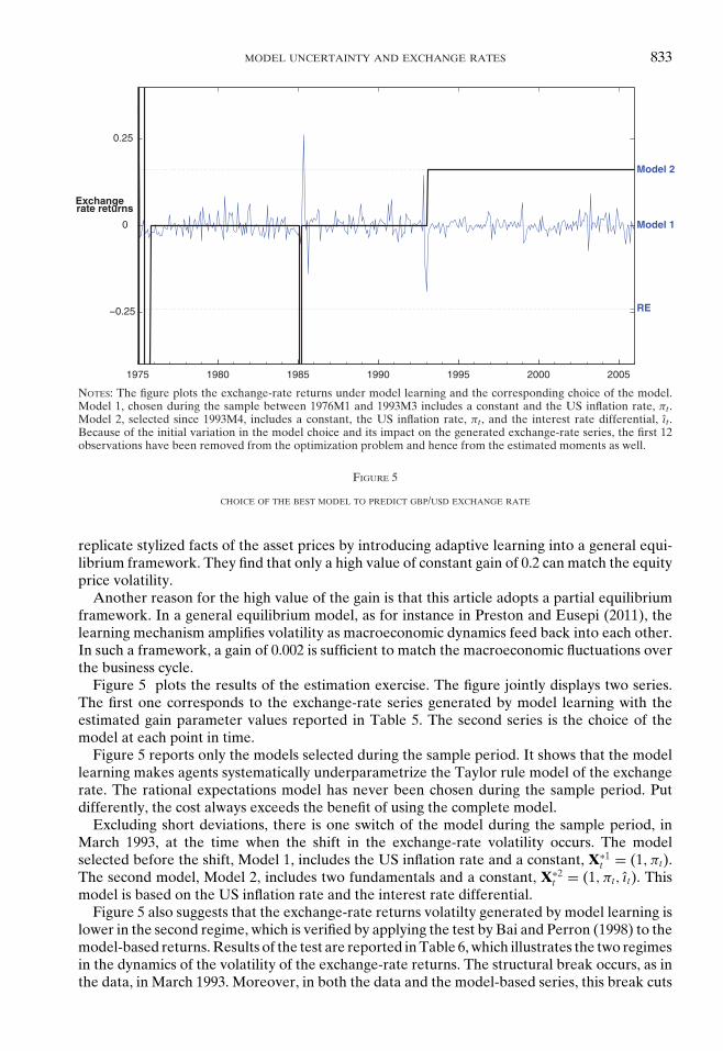
NOTES: The figure plots the exchange-rate returns under model learning and the corresponding choice of the model.Model 1, chosen during the sample between 1976M1 and 1993M3 includes a constant and the US inflation rate, πt .Model 2, selected since 1993M4, includes a constant, the US inflation rate, πt , and the interest rate differential, ıt .Because of the initial variation in the model choice and its impact on the generated exchange-rate series, the first 12observations have been removed from the optimization problem and hence from the estimated moments as well.

FIGURE 5

CHOICE OF THE BEST MODEL TO PREDICT GBP/USD EXCHANGE RATE

replicate stylized facts of the asset prices by introducing adaptive learning into a general equi-librium framework. They find that only a high value of constant gain of 0.2 can match the equityprice volatility.

Another reason for the high value of the gain is that this article adopts a partial equilibriumframework. In a general equilibrium model, as for instance in Preston and Eusepi (2011), thelearning mechanism amplifies volatility as macroeconomic dynamics feed back into each other.In such a framework, a gain of 0.002 is sufficient to match the macroeconomic fluctuations overthe business cycle.

Figure 5 plots the results of the estimation exercise. The figure jointly displays two series.The first one corresponds to the exchange-rate series generated by model learning with theestimated gain parameter values reported in Table 5. The second series is the choice of themodel at each point in time.

Figure 5 reports only the models selected during the sample period. It shows that the modellearning makes agents systematically underparametrize the Taylor rule model of the exchangerate. The rational expectations model has never been chosen during the sample period. Putdifferently, the cost always exceeds the benefit of using the complete model.

Excluding short deviations, there is one switch of the model during the sample period, inMarch 1993, at the time when the shift in the exchange-rate volatility occurs. The modelselected before the shift, Model 1, includes the US inflation rate and a constant, X∗1

t = (1, πt).The second model, Model 2, includes two fundamentals and a constant, X∗2

t = (1, πt, ıt). Thismodel is based on the US inflation rate and the interest rate differential.

Figure 5 also suggests that the exchange-rate returns volatilty generated by model learning islower in the second regime, which is verified by applying the test by Bai and Perron (1998) to themodel-based returns. Results of the test are reported in Table 6, which illustrates the two regimesin the dynamics of the volatility of the exchange-rate returns. The structural break occurs, as inthe data, in March 1993. Moreover, in both the data and the model-based series, this break cuts

834 MARKIEWICZ

TABLE 6

TIMING OF BREAKS IN MODEL BASED EXCHANGE-RATE RETURNS AND IN THE DATA

Volatility of the Exchange-Rate Returns

Model Learning Data

Break date 1993M3 1993M3Regime 1 0.0365 0.0362Regime 2 0.0205 0.0207

NOTES: The first regime corresponds to 1976M1-1993M3 and the second to 1993M4-2008M8. The break date is significantat the 1% confidence level.

the returns into two volatility regimes–the high before the break and the low volatility regimeafter the shift. It is therefore clear that model learning can replicate the volatility dynamics ofBritish pound/US dollar returns.

5.2. Model Learning versus RE and RPEs. I will now compare model learning with fivespecifications: (i) RE structure with constant parameters without smoothing; (ii) RE structurewith constant parameters with interest rate smoothing; (iii) RE structure with time-varyingpolicy rule parameters; (iv) parameter learning within underparametrized specification of Model1; and (v) parameter learning within underparametrized specification of Model 2.

The RE specifications with constant parameters are generated using the fundamentals’monthly data and the estimates displayed in Table 4. The models with time-varying coeffi-cients (RE structure with time-varying policy rule parameters, parameter learning within un-derparametrized specification of Model 1, and parameter learning within underparametrizedspecification of Model 2) are estimated by two-steps GMM. In order to facilitate the comparisonbetween these models, the same data-based weighting matrix is used in the second step of theestimation. The weighting matrix, initial values, and further details of the GMM procedure arereported in Appendix A.5. The estimated parameter values and the actual data on fundamentalsare used to generate the exchange-rate series and to compare the proposed models.

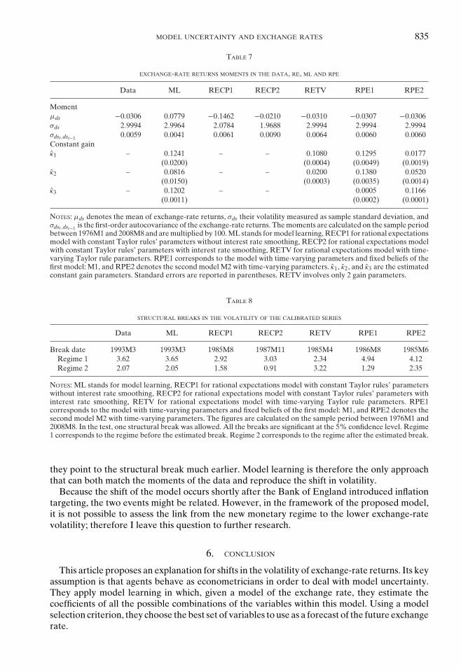
Model learning is compared to the alternative representations in several dimensions. Inparticular, I seek to identify the model that can match the moments in the data defined by (46)and can simultaneously generate the shift in the exchange-rate volatility. Table 7 shows howwell these models match the moments in the data.

The upper part of Table 7 reports the three moments used to estimate the constant gainvalues κ1, κ2, and κ3, which are reported in the lower part of the table. First, note that fourout of six specifications match the exchange-rate volatility. Under the two constant parametersRE models, the volatility is lower than the data indicate. Column 6 of Table 7 entitled RETVshows that using the same fundamentals, one can reach the desired exchange-rate volatility byintroducing learning dynamics. This result was also demonstrated by Kim (2009) and Lewisand Markiewicz (2009). Table 7 also suggests that both the mean and the autocovariances areclose to 0, and they are well matched by most of the models. Table 8 reports the results of thestructural break tests.

As already indicated in the previous section, model learning generates the volatility shiftin March 1993. None of the alternative models can generate returns with a structural shiftin the volatility corresponding to the one found in the data. Table 8 shows that, althoughall series exhibit volatility shifts, none of them occurs in the beginning of 1993. The constantparameters RE models, as already indicated in the previous section, underestimate variability inboth regimes. The time-evolving RE specification surprisingly suggests that the exchange-ratevolatility significantly increased during the sample period. Finally, the two RPE driven modelsdisplay patterns similar to the data as the volatility declines in the sample period. Nevertheless,


TABLE 7

EXCHANGE-RATE RETURNS MOMENTS IN THE DATA, RE, ML AND RPE

Data ML RECP1 RECP2 RETV RPE1 RPE2

Momentμds −0.0306 0.0779 −0.1462 −0.0210 −0.0310 −0.0307 −0.0306σds 2.9994 2.9964 2.0784 1.9688 2.9994 2.9994 2.9994σdst ,dst−1 0.0059 0.0041 0.0061 0.0090 0.0064 0.0060 0.0060Constant gainκ1 – 0.1241 – – 0.1080 0.1295 0.0177

(0.0200) (0.0004) (0.0049) (0.0019)κ2 – 0.0816 – – 0.0200 0.1380 0.0520

(0.0150) (0.0003) (0.0035) (0.0014)κ3 – 0.1202 – – 0.0005 0.1166

(0.0011) (0.0002) (0.0001)

NOTES: μds denotes the mean of exchange-rate returns, σds their volatility measured as sample standard deviation, andσdst ,dst−1 is the first-order autocovariance of the exchange-rate returns. The moments are calculated on the sample periodbetween 1976M1 and 2008M8 and are multiplied by 100. ML stands for model learning, RECP1 for rational expectationsmodel with constant Taylor rules’ parameters without interest rate smoothing, RECP2 for rational expectations modelwith constant Taylor rules’ parameters with interest rate smoothing, RETV for rational expectations model with time-varying Taylor rule parameters. RPE1 corresponds to the model with time-varying parameters and fixed beliefs of thefirst model: M1, and RPE2 denotes the second model M2 with time-varying parameters. κ1, κ2, and κ3 are the estimatedconstant gain parameters. Standard errors are reported in parentheses. RETV involves only 2 gain parameters.

TABLE 8

STRUCTURAL BREAKS IN THE VOLATILITY OF THE CALIBRATED SERIES

Data ML RECP1 RECP2 RETV RPE1 RPE2

Break date 1993M3 1993M3 1985M8 1987M11 1985M4 1986M8 1985M6Regime 1 3.62 3.65 2.92 3.03 2.34 4.94 4.12Regime 2 2.07 2.05 1.58 0.91 3.22 1.29 2.35

NOTES: ML stands for model learning, RECP1 for rational expectations model with constant Taylor rules’ parameterswithout interest rate smoothing, RECP2 for rational expectations model with constant Taylor rules’ parameters withinterest rate smoothing, RETV for rational expectations model with time-varying Taylor rule parameters. RPE1corresponds to the model with time-varying parameters and fixed beliefs of the first model: M1, and RPE2 denotes thesecond model M2 with time-varying parameters. The figures are calculated on the sample period between 1976M1 and2008M8. In the test, one structural break was allowed. All the breaks are significant at the 5% confidence level. Regime1 corresponds to the regime before the estimated break. Regime 2 corresponds to the regime after the estimated break.

they point to the structural break much earlier. Model learning is therefore the only approachthat can both match the moments of the data and reproduce the shift in volatility.

Because the shift of the model occurs shortly after the Bank of England introduced inflationtargeting, the two events might be related. However, in the framework of the proposed model,it is not possible to assess the link from the new monetary regime to the lower exchange-ratevolatility; therefore I leave this question to further research.

6. CONCLUSION

This article proposes an explanation for shifts in the volatility of exchange-rate returns. Its keyassumption is that agents behave as econometricians in order to deal with model uncertainty.They apply model learning in which, given a model of the exchange rate, they estimate thecoefficients of all the possible combinations of the variables within this model. Using a modelselection criterion, they choose the best set of variables to use as a forecast of the future exchangerate.

836 MARKIEWICZ

Using a version of the asset pricing model, the article demonstrates that learning about themodel of the exchange rate may lead agents to focus excessively on a subset of fundamentalvariables at different points in time. By choosing misspecified models, the agents alter the weightplaced on selected fundamental variables relative to others. Because the asset pricing equationhas a self-referential structure, the chosen model feeds back into the actual exchange rate.Consequently, as agents switch between models, the nominal exchange-rate volatility variesaccordingly, even though the underlying fundamentals’ processes remain time-invariant.

The model learning framework was applied to the Taylor rule-based model of the Britishpound/US dollar exchange rate. Model learning as well as alternative time-varying specificationswere estimated by two-steps GMM. The results demonstrate that model learning and a numberof alternative specifications can match moments in the exchange-rate data. In contrast to thealternative models, however, the model learning-based exchange-rate model can replicate theshift in volatility in March 1993.

APPENDIX

A.1. Structural Break Tests. I test for structural breaks using the procedure proposed byBai and Perron (1998, 2003). The test is applied to the absolute value of the demeaned series|dxt − μ|. The sequential procedure is as follows. First, I estimate up to five breaks in the series.Second, I apply the test, which is designed to detect the presence of (j + 1) breaks conditional onhaving found j breaks (j = 0, 1, . . . , 5). The statistical rule is to reject j in favor of a model with (j+ 1) breaks if the overall minimal value of the sum of squared residuals (over all the subsampleswhere an additional break is included) is sufficiently smaller than the sum of squared residualsfrom the model with j breaks. The dates of the selected breaks are the ones associated with thisoverall minimum.

I use the code accompanying the paper by Bai and Perron (2003), which can be found on thewebsite http://people.bu.edu/perron/code.html

Consider the case of the unconditional volatility of the British pound/US dollar returns,where I test for a structural break in the mean of the absolute value of the demeaned series,yt = |dst − μ|. The results of the structural break test for this series are reported in the secondcolumn of Table A.1. I find that there is a break in the volatility of exchange-rate returns inMarch 1993.

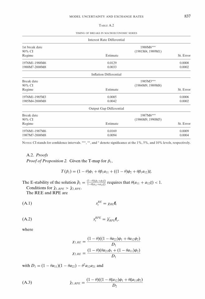
I also test for unconditional volatility shifts in macroeconomic series, namely, interest rate,inflation rate differentials, and output gap differential. I use again the test proposed by Bai andPerron (1998, 2003), which is applied to the absolute value of the demeaned series |dxt − μ|,where dxt is the first difference of inflation rate differential, interest rate differential, and outputgap differential. Table A.2 reports the results.

TABLE A.1

TIMING OF BREAKS IN BRITISH POUND/US DOLLAR RETURNS

Exchange-rate Returns Volatility

Break date 1993M3∗∗∗90% CI (1992M6-1996M7)

Regime Estimate

1976M1-1993M3 0.0362∗∗∗1993M4-2008M8 0.0207∗∗∗

CI stands for confidence intervals. ∗∗∗, ∗∗, and ∗ denote significance at the 1%, 5%, and 10% levels, respectively.


TABLE A.2

TIMING OF BREAKS IN MACROECONOMIC SERIES

Interest Rate Differential

1st break date 1988M6∗∗∗90% CI (1981M4, 1989M1)Regime Estimate St. Error

1976M1-1988M6 0.0129 0.00081988M7-2008M8 0.0033 0.0002

Inflation Differential

Break date 1985M3∗∗∗90% CI (1984M9, 1989M8)Regime Estimate St. Error

1976M1-1985M3 0.0085 0.00061985M4-2008M8 0.0042 0.0002

Output Gap Differential

Break date 1987M6∗∗∗90% CI (1986M9, 1990M5)Regime Estimate St. Error

1976M1-1987M6 0.0169 0.00091987M7-2008M8 0.0094 0.0004

NOTES: CI stands for confidence intervals. ∗∗∗, ∗∗, and ∗ denote significance at the 1%, 5%, and 10% levels, respectively.

A.2. ProofsProof of Proposition 2. Given the T-map for β1,

T (β1) = (1 − θ)φ1 + θβ1a11 + ((1 − θ)φ2 + θβ1a12)ξ.

The E-stability of the solution β1 = (1−θ)(φ1+φ2ξ)1−θ(a11+a12ξ) requires that θ(a11 + a12ξ) < 1.

Conditions for χ1,RPE > χ2,RPE.The REE and RPE are

sREt = χREft(A.1)

sRPEt = χ′

RPEf t,(A.2)

where

χ1,RE = (1 − θ)((1 − θa22)φ1 + θa12φ2)D1

χ2,RE = (1 − θ)(θa21φ1 + (1 − θa11)φ2)D1

with D1 = (1 − θa11)(1 − θa22) − θ2a12a21 and

χ1,RPE = (1 − θ)((1 − θξa12)φ1 + θξa11φ2)D2

(A.3)

838 MARKIEWICZ

χ2,RPE = (1 − θ)(θa12φ1 + (1 − θa11)φ2)D2

,(A.4)

where D2 = 1 − θ(a12ξ + a11) and ξ = Ef 1f 2

Ef 21

. Under the assumption that φ1 = φ2, a11 = a22, and

a12 = a21, (1 − θa22)φ1 + θa12φ2 = θa21φ1 + (1 − θa11)φ2 and hence χ1,RE = χ2,RE. In this specialcase, the RPE coefficients imply (1 − θξa12)φ1 + θξa11φ2 > θa12φ1 + (1 − θa11)φ2 if a11 > a12.

A.3. Derivation of the Taylor Rule Model of the Exchange Rate

Taylor rule model of the exchange rate without interest rate smoothing. The home centralbank follows the Taylor rule

ıt = a0 + a1πt + a2yt + vt.(A.5)

The foreign central bank follows the rule that also includes the real exchange rate

ı∗t = a∗0 + a∗

1π∗t + a∗

2y∗t + a∗

3qt + v∗t ,(A.6)

where qt = p t − st and p t =pt − p∗t . The UIP condition is

it = i∗t + Etst+1 − st + ut,(A.7)

where ut is an exogenous risk premium shock. The market interest rate at home is it = ıt + τt

and abroad i∗t = ı∗t + τ∗t . Substruct the foreign Taylor rule (A.6) from the home Taylor rule

(A.5):

it − i∗t = a0 + a1πt + a2yt − a∗0 − a∗

1π∗t − a∗

2y∗t − a∗

3qt + vt − v∗t + τt − τ∗

t .

Use UIP in (A.7) to obtain the following:

Etst+1 − st + ut = a0 + a1πt + a2yt − a∗0 − a∗

1π∗t − a∗

2y∗t − a∗

3 p t

+ a∗3

(Etst+1 − (

it − i∗t) + ut

) + vt − v∗t + τt − τ∗

t .

One can write this specification in the following asset pricing equation form:

st = (1 − θ)φ′ft + θEtst+1 + εt,(A.8)

where θ = (1 − a∗3), φ′ = ( a0

a∗3, − a1

a∗3, − a2

a∗3,

a∗1

a∗3,

a∗2

a∗3, 1, 1 ), and f ′

t = ( 1, πt, yt, π∗t, y∗

t , ıt p t ),a0 = a∗

0 − a0, p t = pt − p∗t , ıt = it − i∗t , and εt = (ν∗

t − νt) + (τ∗t − τt) + ut(1 − a∗

3).

Taylor rule model of the exchange rate with interest rate smoothing component. The homecentral bank follows the Taylor rule:

ıt = (1 − ρ)(a0 + a1πt−1 + a2yt−1) + ρıt−1 + vt.(A.9)

The foreign central bank follows the rule that also includes the real exchange rate


ı∗t = (1 − ρ∗)(a∗

0 + a∗1π

∗t−1 + a∗

2y∗t−1 + a∗

3qt−1) + ρ∗ ı∗t−1 + v∗

t(A.10)

where qt = p t − st. Substruct the foreign Taylor rule (A.10) from the home Taylor rule (A.9),use UIP in (A.7) and set ρ = (ρ + ρ*)/2 to obtain the following:

st = (1 − θ)φ′ft + θEtst+1 + εt,

where θ = 1/(1 + (1 − ρ)a∗3), φ′ = ( a0

a∗3, −a1

a∗3

, −a2a∗

3,

a∗1

a∗3,

a∗2

a∗3, − ρ

(1−ρ)a∗3, 1 ), and f ′

t = (1, πt, yt,

π∗t , y∗

t , ıt, p t), a0 = a∗0 − a0, p t = pt − p∗

t , ıt = it − i∗t , and εt = (ν∗t − νt) + (τ∗

t − τt) + ut.

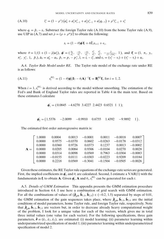
A.4. Taylor Rule Model under RE. The Taylor rule model of the exchange rate under REis as follows:

sREit = (1 − θ)φ′

i(I7 − θiA)−1ft = BREi ft, for i = 1, 2.(A.11)

When i = 1, sRE1t is derived according to the model without smoothing. The estimation of the

Fed’s and Bank of England Taylor rules are reported in Table 4 in the main text. Based onthese estimates I calculate

φ′1 = ( 0.0845 −4.6270 3.4227 2.4423 0.6521 1 1 );

φ′2 = (

1.5376 −2.0099 −0.9910 0.6755 1.4392 −9.9892 1).

The estimated first order autoregressive matrix is:

A =

⎡⎢⎢⎢⎢⎢⎢⎢⎢⎣

1.0000 0.0004 0.0013 −0.0001 0.0011 −0.0018 0.00070.0000 0.9575 −0.0370 0.0602 −0.0263 −0.0178 −0.03120.0000 0.0360 0.9726 0.0373 0.1237 0.0013 −0.00020.0000 0.0205 0.0084 0.9306 −0.0104 0.0270 0.00280.0000 0.0314 0.0098 0.0569 0.7963 −0.0304 −0.00830.0000 −0.0155 0.0111 −0.0303 −0.0223 0.9209 0.01840.0000 0.2218 0.0569 −0.3041 −0.1504 −0.0505 −0.0026

⎤⎥⎥⎥⎥⎥⎥⎥⎥⎦Given these estimates, the RE Taylor rule equations of the exchange-rate series are generated.

First, the implied coefficients in φ′i, and θi are calculated. Second, I estimate a VAR(1) with the

fundamentals in ft to obtain A. Given φ′i, A and θi, sREi

t can be generated for each t.

A.5. Details of GMM Estimation This appendix presents the GMM estimation procedureintroduced in Section 4.4. I use here a combination of grid search with GMM estimation.For all the combinations of values of (βj,0, b1,0, b2,0) ∈ (−0.2, 1.5) separated by steps of 0.01,the GMM estimation of the gain sequences takes place, where βj,0, b1,0, b2,0 are the initialconditions of model parameters, home Taylor rule, and foreign Taylor rule, respectively. Notethat βj,0, b1,0, b2,0 are vectors but, in order to decrease already heavy computational weightof the problem, I look for a unique value for each of the vectors, which gives me in totalthree initial values (one value for each vector). For the following specifications, three gainparameters, θ ≡ (κ1, κ2, κ3), are estimated: (i) model learning; (ii) parameter learning withinunderparametrized specification of model 1; (iii) parameter learning within underparametrizedspecification of model 2.

840 MARKIEWICZ

The moment conditions are given by

m =⎡⎣ μds − μ∗

dsσds − σ∗

dsσdst,dst−1 − σ∗

dst,dst−1

⎤⎦ ,

where the moments with asterisks correspond to the ones derived from the model.The RE structure with time varying parameters of monetary policy rules needs only two gain

parameters to be estimated, θ ≡ (κ1, κ2). Also, because there is no models’ parameter learningin this specification, initial values only include two parameters (b1,0, b2,0) and only two firstmoments, m = [μds − μ∗

ds, σds − σ∗ds]

′ are used to estimate the gains’ vector θ.The GMM estimator is defined as

θ ≡ arg minθ

m′W m,(A.12)

where W is assumed to be identity matrix I3. This first step estimation provides consistentestimates of the true θ. In the second step I use the diagonal matrix W with the inverse of thestandard deviations of the data moments, 1

σsi, on the diagonal. The data-based moments are

chosen to facilitate the comparison between the models. Instead of a full (efficient) weightingmatrix, the diagonal was selected as in many finite sample applications of GMM (e.g., Andersenand Sorensen, 1994). In the estimation of all three gains, θ ≡ (κ1, κ2, κ3), the following matrix isused in the second step:

W =⎡⎣ 33.0481 0 0

0 46.7370 00 0 663.4364

⎤⎦ ,

where the highest weight is put on the third moment, the first order autocovariance, because itsvolatility is the lowest. Using this weighting matrix, W, the second step estimates are computed

θ ≡ arg minθ

m′Wm.

The standard errors of θ are computed using the delta method, and they are reportedin Tables 5 and 7 of the main text. This estimation procedure is carried for all the initialvalues combinations of (βj,0, b1,0, b2,0) ∈ (−0.2, 1.5). Optimal initial values are reported inTable A.3.

TABLE A.3

OPTIMAL INITIAL VALUES IN THE GMM ESTIMATIONS

ML RETV RPE1 RPE2

Initial valueβj,0 0.71 – −0.20 −0.20b1,0 0.37 1.50 0.04 −0.20b2,0 0.64 0.53 0.77 1.50

NOTES: ML stands for model learning and RETV for rational expectations model with time-varying Taylor ruleparameters. RPE1 corresponds to the model with time-varying parameters and fixed beliefs of the first model: M1, andRPE2 denotes the second model M2 with time-varying parameters. βj,0, b1,0, and b2,0 are the optimal initial values.


A.6. Data

TABLE A.4

DESCRIPTION OF THE DATA SOURCES AND THE CONSTRUCTION OF VARIABLES

Variable Country Measure Source

Exchange rate USD/GBP Market rate: end of the month IFSInterest rate US 1-Month Certificate of Deposit: Secondary Market Rate FREDInterest rate UK 3-Month UK Treasury Bill Discount Rate BoEOutput US Total Industrial Production, s.a., 2002 = 100 FedOutput UK Total Industrial Production, s.a., 2005 = 100 ONS

Output gap US yg∗t = y∗

t − yHP∗(a)t Fed+(a)

Output gap UK ygt = yt − yHP(a)

t ONS+(b)

Prices US Consumer Price Index (CPI) IFSPrices UK Consumer Price Index (CPI) IFSInflation US First difference of log of CPI ONSInflation UK First difference of log CPI BLS

NOTES: The sample for all the series is from 1973M1 to 2009M1. FRED: Federal Reserve Economic Data, BoE: Bankof England, Fed: Federal Reserve Board, ONS: Office for National Statistics, and BLS: Bureau of Labor Statistics.(a)

Output gap is calculated as deviations of actual output from the H-P trend, which was constructed recursively.(b)Author’s calculations.

REFERENCES

ADAM, K., A. MARCET, AND J. P. NICOLINI, “Stock Market Volatility and Learning,” Mimeo, University ofManheim, 2009.

ANDERSEN, T. G., AND B. E. SORENSEN, “Estimation of a Stochastic Volatility Model: A Monte CarloStudy,” Journal of Business and Economic Statistics 14 (1994), 328–52.

ARIFOVIC, J., “The Behavior of the Exchange Rate in the Genetic Algorithm and ExperimentalEconomies,” The Journal of Political Economy 104 (1996), 510–41.

BACCHETTA, P., AND E. VAN WINCOOP, “A Scapegoat Model of Exchange Rate Fluctuations,” AmericanEconomic Review, Papers and Proceedings 94 (2004), 114–8.

BAI, J., AND P. PERRON, “Estimating and Testing Linear Models with Multiple Structural Changes,”Econometrica 66 (1998), 47–78.

———, AND ———, “Computation and Analysis of Multiple Structural Change Models,” Journal ofApplied Econometrics 18 (2003), 1–22.

BALL, L., “Policy Rules for Open Economies” in J. B. Taylor, ed., Monetary Policy Rules (Chicago:University of Chicago Press, 1999), 127–44.

BAXTER, M., AND A. C. STOCKMAN, “Business Cycles and the Exchange-Rate Regime,” Journal of MonetaryEconomics 23 (1989), 377–400.

BILSON, J., “The Monetary Approach to the Exchange Rate: Some Empirical Evidence,” IMF Staff Papers25 (1978), 48–75.

BOZ, E., C. DAUDE, AND C. B. DURDU, “Emerging Market Business Cycles Revisited: Learning About theTrend,” Journal of Monetary Economics 58 (2011), 616–31.

BRAILSFORD, T. J., J. H. W. PENM, AND R. D. TERRELL, “Selecting the Forgetting Factor in Subset Autore-gressive Modelling,” Journal of Time Series Analysis 23 (2002), 629–49.

BRANCH, W., AND G. W. EVANS, “A Simple Recursive Forecasting Model,” Economics Letters 91 (2006a),158–66.

———, AND ———, “Intrinsic Heterogeneity in Expectation Formation,” Journal of Economic Theory127 (2006b), 264–95.

———, AND ———, “Model Uncertainty and Endogenous Volatility,” Review of Economic Dynamics 10(2007), 207–37.

BRAY, M., “Learning, Estimation, and the Stability of Rational Expectations,” Journal of Economic Theory26 (1982), 318–39.

———, AND E. SAVIN., “Rational Expectations Equilibria, Learning and Model Selection,” Econometrica54 (1986), 1129–60.

CARCELES-POVEDA, E., AND C. GIANNITSAROU, “Asset Pricing with Adaptive Learning,” Review of Eco-nomic Dynamics 11 (2008), 629–51.

842 MARKIEWICZ

CHEUNG, Y.-W., M. D. CHINN, AND A. G. PASCUAL, “Empirical Exchange Rate Models of the Nineties: AreAny Fit to Survive?” Journal of International Money and Finance 24 (2005), 1150–75.

CHEVILLON, G., M. MASSMANN, AND S. MAVROEIDIS, “Inference in Models with Adaptive Learning,” Journalof Monetary Economics 57 (2010), 341–51.

CHO, I.-K., AND K. KASA, “Learning and Model Validation,” Mimeo, Simon Fraser University,2008.

CLARIDA, R., AND D. WALDMAN, (2007) “Is Bad News about Inflation Good News for the Exchange Rate?”in J. Campbell, ed., Asset Prices and Monetary Policy (Chicago: University of Chicago Press, 2008),371–96.

———, J. GALI, AND M. GERTLER, “Monetary Rules in Practice: Some International Evidence,” EuropeanEconomic Review, 6 (1998), 1033–67.

ENGEL, C., AND J. D. HAMILTON, “Long Swings in the Dollar: Are They in the Data and Do Markets KnowIt?” American Economic Review 80 (1990), 689–713.

———, AND K. D. WEST, “Exchange Rate and Fundamentals,” Journal of Political Economy 113 (2005),485–517.

———, AND ———, “Taylor Rules and the Deutschmark-Dollar Real Exchange Rate,” Journal of Money,Credit, and Banking 38 (2006), 1175–94.

EVANS, G. W., AND W. BRANCH, “Asset Return Dynamics and Learning,” Review of Financial Studies 23(2010).

———, AND A. CHAKRABORTY, “Can Perpetual Learning Explain the Forward Premium Puzzle,” Journalof Monetary Economics 55 (2008), 477–90.

———, AND S. HONKAPOHJA, Learning and Expectations in Macroeconomics (Princton: Princeton Univer-sity Press, 2001).

FLOOD, R., AND A. ROSE, “Fixing Exchange Rates: A Virtual Quest for Fundamentals,” Journal of MonetaryEconomics 36 (1995), 3–38.

FRENKEL, J., “A Monetary Approach to the Exchange Rate: Doctrinal Aspects and Empirical Evidence,”Scandinavian Journal of Economics 78 (1976), 200–24.

GERLACH, S., “World Business Cycles Under Fixed and Flexible Exchange Rates,” Journal of Money,Credit, and Banking 20 (1988), 621–32.

GOURINCHAS, P. O., AND A. TORNELL, “Exchange Rate Puzzles and Distorted Beliefs,” Journal of Interna-tional Economics 64 (2004), 303–33.

HANSEN, L., AND T. SARGENT, “Acknowledging Misspecification in Macroeconomic Theory,” Review ofEconomic Dynamics 4 (2001), 519–35.

HODRICK, R., AND E. PRESCOTT, “Postwar U.S. Business Cycles: An Empirical Investigation,” Journal ofMoney, Credit, and Banking 29 (1997), 1–16.

HOOPER, P., AND J. MORTON, “Fluctuations in the Dollar: A Model of Nominal and Real Exchange RateDetermination,” Journal of International Money and Finance 1 (1982), 39–56.

HUANG, K., Z. LIU, AND T. ZHA, “Learning, Adaptive-Expectations, and Technology Shocks,” EconomicJournal 119 (2009), 377–405.

JEANNE, O., AND A. ROSE, “Noise Trading and Exchange Rate Regimes,” Quarterly Journal of Economics117 (2002), 537–69.

KIM, Y. S., “Exchange Rates and Fundamentals under Adaptive Learning,” Journal of Economic Dynamicsand Control 33 (2009), 843–63.

LEWIS, K., “Can Learning Affect Exchange Rate Behavior? The Case of the Dollar in the Early 1980’s,”Journal of Monetary Economics 23 (1989a), 79–100.

———, “Changing Beliefs and Systematic Rational Forecast Errors with Evidence from Foreign Ex-change,” American Economic Review 79 (1989b), 621–36.

LEWIS, V., AND A. MARKIEWICZ, “Misspecification, Learning and the Exchange Rate Disconnect Puzzle,”The B.E. Journal of Macroeconomics (Topics) 9 (2009), 1–22.

LUBIK, T., AND S. FRANK, “Do Central Banks Respond to Exchange Rate Movements? A StructuralInvestigation,” Journal of Monetary Economics 54 (2007), 1069–87.

LUTKEPOHL, H., “Comparison of Criteria for Estimating the Order of a Vector Autoregressive Process,”Journal of Time Series Analysis 6 (1985), 35–52.

MARCET, A., AND T. SARGENT, “Convergence of Least Squares Learning Mechanisms in Self-ReferentialLinear Stochastic Models,” Journal of Economic Theory 48 (1989), 337–68.

MARK, N., “Changing Monetary Policy Rules, Learning, and Real Exchange Rate Dynamics,” Journal ofMoney, Credit, and Banking 41 (2009), 1047–70.

MILANI, F., “Expectations, Learning and Macroeconomic Persistence,” Journal of Monetary Economics54 (2007a), 2065–82.

———, “Learning and Time-varying Macroeconomic Volatility,” Mimeo, University of California,(2007b).

MILLS, J., AND K. PRASAD, “Comparison of Model Selection Criteria,” Econometric Reviews 11 (1992),201–33.


MOLODTSOVA, T., AND D. PAPELL, “Out-of-Sample Exchange Rate Predictability with Taylor Rule Funda-mentals,” Journal of International Economics 77 (2010), 137–276.

MUSSA, M., “Empirical Regularities in the Behaviour of Exchange Rates and Theories of the ForeignExchange Market,” Carnegie-Rochester Series on Public Policy 11 (1979), 9–58.

———, “Nominal Exchange-Rate Regimes and the Behavior of Real Exchange Rates: Evidence andImplications,” Carnegie-Rochester Series on Public Policy 25 (1986), 117–214.

NELSON, E., “UK Monetary Policy 1972-97: A Guide Using Taylor Rules,” CEPR Discussion Papers No.2931, C.E.P.R., London, 2001.

ORPHANIDES, A., AND J. WILLIAMS, “Imperfect Knowledge, Inflation Expectations, and Monetary Policy,”In B.S. Bernanke and M. Woodford, eds., The Inflation Targeting Debate (Chicago: University ofChicago Press, 2004), 201–46.

———, AND ———, “The Decline of Activist Stabilization Policy: Natural Rate Misperceptions, Learning,and Expectations,” Journal of Economic Dynamics and Control 29 (2005), 1927–50.

PESARAN, M. H., AND A. PICK, “Forecast Combination over Estimation Windows,” Journal of Businessand Economic Statistics 29 (2011), 307–18.

PRESTON, B., AND S. EUSEPI, “Expectations, Learning and Business Cycle Fluctuations,” American Eco-nomic Review 101 (2011), 2844–72.

ROSSI, B., “Are Exchange Rates Really Random Walks? Some Evidence Robust to Parameter Instability,”Macroeconomic Dynamics 10 (2006), 20–38.

SARGENT, T., Bounded Rationality in Macroeconomics (New York: Oxford University Press, 1993).SARNO, L., AND G. VALENTE, “Exchange Rates and Fundamentals: Footloose or Evolving Relationship?”

Journal of European Economic Association 7 (2009), 786–830.SCHINASI, G., AND P. A. V. B. SWAMY, “The Out-of-Sample Forecasting Performance of Exchange Rate

Models When Coefficients Are Allowed to Change,” Journal of International Money and Finance 8(1989), 375–90.

SCHWARZ, G., “Estimating the Dimension of a Model,” Annals of Statistics 6 (1978), 461–4.SINHA, A., “Learning and the Yield Curve,” Mimeo, Columbia University, 2009.SVENSSON, L., “Open Economy Inflation Targeting,” Journal of International Economics 50 (2000), 155–

83.TAYLOR, J., Monetary Policy Rules (Chicago: University of Chicago Press, 1999).

model uncertainty and exchange rate volatility

Documents