1

CSI RD&D3 Subtask 4.4 Final Report:

Model Predictive On-Load Tap Changer Control for High Penetrations of PV Using Sky Imager Solar Forecast

Submitted to:

Stephan Barsun, P.E. Principal Energy Consultant, Itron

California Solar Initiative RD&D Program

October 2015

Submitted by:

Vahid Disfani, Pablo Ubiratan, Jan Kleissl

Department of Mechanical and Aerospace Engineering Jacobs School of Engineering

Center for Renewable Resource Integration and Center for Energy Research University of California, San Diego

9500 Gilman Drive La Jolla, CA 92093-0411, USA

Abstract

A control strategy to reduce OLTC operations resulting from high PV penetration on distribution feeders was developed and applied. The strategy uses 5 minutes ahead solar forecast to derive future voltages states on the distribution feeder. Unnecessary TO are identified as those that are reversed within 5 minutes, likely because of temporary cloudy or clear conditions over adjacent PV systems. Unnecessary TO are eliminated.

On a feeder where TO were abundant at over 750 per day on average, the strategy resulted in the avoidance of 56% of the TO, which would result in significant savings in OLTC maintenance costs. Average extreme voltages were not affected by applying the TO reduction techniques. While daily maximum/minimum voltage excursions over the entire feeder slightly increased on several days, a statistical analysis demonstrated that these deviations happened very rarely.

The strategy is most effective on partly cloudy days and on voltage regulators with a large number of TO. The fraction of avoided TO decreased substantially for less than 10 to 40 TO per day, depending on the voltage regulator. The control algorithm was shown to be robust against forecast errors inherent in state-of-the art sky imager forecasts.

2

Model Predictive On-Load Tap Changer Control for High Penetrations of PV Using Sky Imager Solar Forecast

I. INTRODUCTION

A. Background

The exponential increase in renewable energy resources such as solar PV systems has introduced different challenges to the operation of electrical distribution systems. As discussed in Task 4.3 of this contract, for higher penetration of solar PV, their variable power output can cause severe voltage fluctuations in the power grid. In order to reduce such voltage variations, transformers and voltage regulators are equipped with On-Load Tap Changers (OLTC) which are programmed to change their tap position to keep voltage levels along the feeder within permissible limits. However, there are some concerns with the operation of OLTCs while performing tap changes.

The main part of an OLTC is the diverter switch which is responsible for effectively managing the tap operation (TO) process without disconnecting the current flow of the transformer. Therefore, switching arcs are inevitable on the main switching and transition contacts of the diverter switch. These arcs create carbonization of the switching oil and cause contact wear. Since diverter switches operate within 40 to 50 milliseconds, the mechanical elements such as springs, braided contact leads etc. are exposed to remarkable stress during every single tap changing event.

For a TO process where the tap position is supposed to change by more than one step, the diverter switch is not able to skip the intermediate steps. Instead, it starts from the initial position and gradually moves through the intermediate steps until it settles on the final position. Thus, the stress on the inverter switch is a function of not only the number of distinct TO, but also the number of taps changed in one operation which is identified as TO depth, hereafter.

According to the mechanical and electrical stresses which OLTC experiences in each TO, the number of TO is one of the main parameters to define the maintenance schedule of OLTC. For example, in [1]-[2], preventive maintenance is recommended to be performed on the tap changer after one million TO. However, it is also stated in [2] that the number of TO must not exceed 500,000 in any case due to weakening spring tensions of the contacts. The other parameter that impacts the OLTC maintenance schedule is the maximum total operation time of OLTC which varies between five and seven years depending on the climate condition.

The variable power output of PV systems through its effect on grid voltage causes a higher volume of TO. Therefore, an investigation has been performed on the number of TO as one of the parameters affecting the distribution system operation in Task 4.3 of this contract. There, the project team showed that for some feeders a higher number of TO is required to maintain the voltage within the limits for higher penetration of PV. In this report, further study is carried out to develop an algorithm to reduce the number of TO by employing solar forecast information to decrease the operation and maintenance (O&M) costs of OLTC.

B. Literature Review

Since TO are costly, most OLTC are designed to only react to persistent exceedances of ANSI voltage limits (plus or minus 5% of the nominal voltage, or 0.95 and 1.05 p.u.). Therefore, delays are introduced with two different time scales: (a) A ‘trigger’ time from when the voltage first reaches the setpoint until the OLTC action. The typical value for this delay is 30 seconds. This intentional delay is considered to make sure that the voltage deviation is persistent or will be removed automatically due to either removal of its cause or action of other voltage regulation devices. (b) An ‘intertap’ delay which is due to the mechanical process that happens inside OLTC to change the tap position by one tap. This delay is typically 2 to 10 seconds based on the type of OLTC. So, the operating time from start to end of the TO is proportional to the depth of TO.

As mentioned, frequent changes in the PV power output are expected in partly cloudy weather condition. If the OLTC operation control is designed just based on the realtime generation of PV, dramatic, but temporary changes in PV output may impose a high-depth operation of OLTC. In addition, the intertap delay may cause the tap operation to be ‘out of synch’ with the PV generation variability. In other words, the change from cloudy to clear may occur over a similar time scale as the TO thereby eliminating the need for the TO or in some cases even exacerbating voltage conditions after the change in cloud cover. For example, there are normally 32 tap positions available on OLTC

3

connected to feeder A. Therefore, an OLTC cannot change the tap position by more than 10 taps assuming a 3-second intertap delay.

The effects of PV generation on the feeder parameters such as power loss and voltage deviation are reported in several works in the literature [3]-[6]. The voltage problem was reported in 2001 in [4] stating that the installation of PV generators always causes a rise in the voltage profile because it leads to reduction of net power load on substation. These rises might cause overvoltage and must be considered in definition of how much PV can be connected to the grid, which is nowadays known as feeder hosting capacity. It is also shown in [5] that high penetration of PV cause voltage rise and overvoltage in rural feeders due to their long line length. The magnitude of voltage rise depends primarily on the feeder impedance, the feeder length, and transformer impedance as demonstrated via simulations in [6]. A steady-state analysis is performed in [7] to determine the hosting capacity of a feeder based on the voltage profile for different PV location scenarios. Another impact of PV on the feeder can be an increase in the number of TO on the OLTCs due to high variability of PV generation. This effect is analyzed in Task 4.3 of this contract.

The literature also includes different solutions to the voltage deviation caused by high penetration of PV such as On-Load Tap Changers (OLTC), State VAR Compensators (SVC), and smart inverters. Three types of voltage regulation devices are commonly used on distribution system: Load Tap Changers (LTC) which is the same as OLTC, switched capacitors, and Voltage Regulators (VREG) [8]. A delay-based control method has been proposed in [9] for LTC to avoid the high number of TO at high penetration of PV. The method proposed applies a 30-second delay between the first time that the controller measures overvoltage on transformer and the time TO starts. This delay, which could be inverse or constant time, allows the LTC to evaluate if the voltage deviation is persistent or it is recovered automatically in order to avoid unnecessary TO during shorter voltage deviations from the target value and to coordinate with other automatic voltage controllers in the system [10].

In [11], an optimization based coordination method between OLTC and SVC is proposed, where the problem is solved in a day-ahead manner. The optimization model determines hourly TO for each OLTC and the intra-hour voltage regulation is performed by SVC considering a typical daily profile for PV power output. The effect of smart inverters on the voltage quality of distribution feeders with high penetrations of PV are studied in [12], [13]. Both works have investigated different control methods such as constant power factor, variable power factor, volt/var control, and voltage regulation to evaluate smart inverter capabilities of mitigating distribution feeder over voltages.

C. Scope of the Report

In this report, a predictive control method is represented to decrease the number/depth of TO using the PV forecast data gathered from sky imagers. Instead of delaying the OLTC action by 30-second (as proposed in [3]), our method employs the sky imager data to immediately define the optimal TO to perform. Since the sky-imager data [14] is available for the next 15 minutes with 30-second resolution, the decision horizon could be set from 30 seconds to 15 minutes. The simulations performed for this report are based on a 5-minute decision horizon. In order to study the effects of forecast error, the algorithm is repeated using the actual PV outputs at [Ts, Ts + 5] (also known as perfect forecast at Ts) instead of actual forecast at Ts.

The rest of the report is organized as following. The problem is stated in Section II. Section III describes the proposed control algorithm. The simulation results are discussed in Section IV, and Section V concludes the report.

II. PRIOR DSS ANALYSIS AND PROBLEM STATEMENT

The variation of the power output from PV arrays, particularly at high penetration levels, may cause serious voltage fluctuations on the feeder. To compensate such voltage variations and prevent them from exceeding the ANSI voltage limits, OLTCs are often implemented. In Task 4.3 of this contract, it was shown that high PV penetration on a feeder may impose a high volume of switching operation on the voltage regulation devices, especially transformer OLTCs. As an example, Fig. 1 shows the mean value of total TO depth per day for five feeders that are characterized in Table I. Feeder A experiences a very high increase in the number of TO in comparison to the other feeders due to its larger number of transformers and voltage regulators (Table I) as well as larger voltage variability as shown in Fig. 2. There are barely any TO on feeder B even at 200% PV penetration since the feeder stiffness causes small voltage variability. For feeder C, D, and E TO increase from 1, 13, and 30 per day at 0% penetration to 4, 30, and 100 per day at 200% penetration.

4

Table I: Characteristics of distribution feeders. Circuit A B C D E

Feeder length (km) 177.8 39.6 34.9 51.5 115.7 No. of Loads 1733 584 471 468 1178 Total peak load (MW) 11.1 8.3 4.8 3.7 5.9 No. of Capacitor banks 5 0 0 0 0 No. of Transformers & VRs 7 1 2 2 2 No. of PV systems (in 2012) 45 85 28 19 43 No. of PV systems (simulated) 432 340 364 104 387 Total rated PV capacity (MWAC in 2012)

2.3 1.3 2.1 0.2 0.3

Large PV systems (#>0.5MW) 2 0 0 2 0 PV penetration in 2012 (%) 18% 15% 58% 4% 4%

Fig. 1. Average of total TO depth per day during daytime. At 0% penetration feeders A, B, C, D, and E have 336, 0, 1, 12, 31 TO, respectively. The number of TO for feeders A, B, and C in the single and multiple scenarios are identical and independent of PV penetration level. An

additional TO may occur at night, but these are not considered here.

Fig. 2. Maximum and minimum voltages on 90 days during day time for feeder A at different penetration levels.

It is reported in the literature [2] that the number of TO of diverter switches for power transformers is approximately 20 per day, which makes the replacement of the contacts unnecessary during the life of transformers. The high number

5

of TO for feeder A, which exceeds 250 TO/day per OLTC on average, makes this feeder an interesting case to study the performance of the model predictive algorithm on both number/depth of TO and voltage quality.

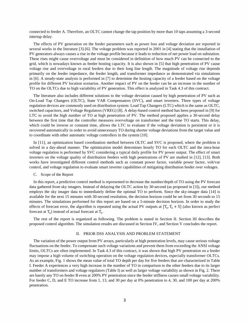
Fig. 3(a) shows feeder A with the location and sizes of actual PV systems as of 2012, while Fig. 3(b) illustrates the virtual PV panels for simulation of higher PV penetration levels. As of 2012 (the last date when real PV interconnection data were available) feeder A which is shown in Fig. 3(a) had two large 1 MW PV systems at the end of the feeder plus 43 small-scale PV systems. About half of these small-scale PV panels are connected close to the end of the feeder while the other half are connected fairly close to the substation. To create a realistic scenario of the future configuration of the feeder with higher PV penetration, new small-scale PV systems are connected to the load points of the feeder. Therefore, the total number of PV systems on this feeder is increased to 432 PV systems including the two large ones. Fig. 3(a) depicts the feeder A with all the real and virtual PV systems. To increase PV penetration level, the size of large-scale PV systems are kept constant while the size of other PV systems are adjusted to create the desired penetration level. This feeder has 7 transformers equipped with 32-step OLTCs with minimum and maximum ratios of 0.9 and 1.1. The network is also equipped with five capacitors. Two capacitors consist of 20 switchable capacitors each while the last three are fixed ones that are always connected to the grid.

(a) (b) Fig. 3. Feeder A showing locations and sizes of (a) actual PV systems as of 2012 and (b) virtual PV panels

connected to the load points to simulate different PV penetration levels.

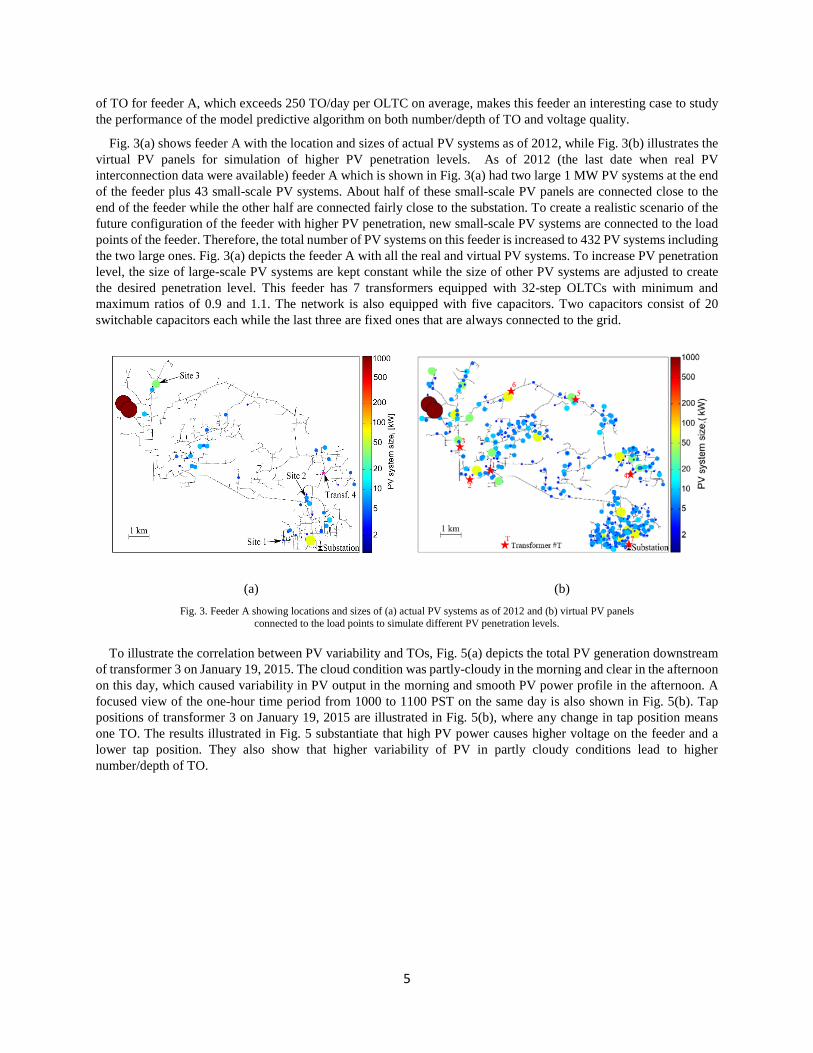
To illustrate the correlation between PV variability and TOs, Fig. 5(a) depicts the total PV generation downstream of transformer 3 on January 19, 2015. The cloud condition was partly-cloudy in the morning and clear in the afternoon on this day, which caused variability in PV output in the morning and smooth PV power profile in the afternoon. A focused view of the one-hour time period from 1000 to 1100 PST on the same day is also shown in Fig. 5(b). Tap positions of transformer 3 on January 19, 2015 are illustrated in Fig. 5(b), where any change in tap position means one TO. The results illustrated in Fig. 5 substantiate that high PV power causes higher voltage on the feeder and a lower tap position. They also show that higher variability of PV in partly cloudy conditions lead to higher number/depth of TO.

6

Fig 4: Simulation results for feeder A at 100% penetration level on Jan 19, 2015 with 30-second resolution, along

with a zoom into an especially variable period from 1000 to 1100 PST. (top) Total power output of 39 PV systems installed downstream of transformer 3. These 39 PV systems form 27% of total PV size on the feeder since both large PV systems are downstream of transformer 3. (bottom) Tap position sequence of transformer 3.

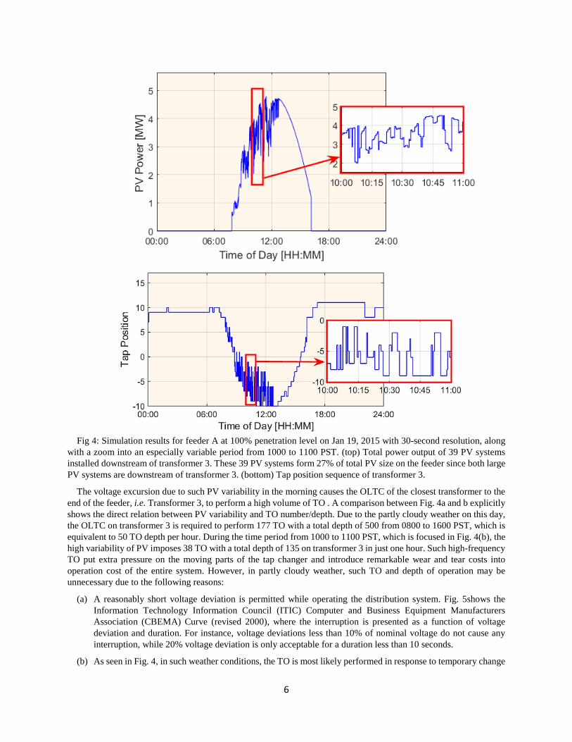
The voltage excursion due to such PV variability in the morning causes the OLTC of the closest transformer to the end of the feeder, i.e. Transformer 3, to perform a high volume of TO . A comparison between Fig. 4a and b explicitly shows the direct relation between PV variability and TO number/depth. Due to the partly cloudy weather on this day, the OLTC on transformer 3 is required to perform 177 TO with a total depth of 500 from 0800 to 1600 PST, which is equivalent to 50 TO depth per hour. During the time period from 1000 to 1100 PST, which is focused in Fig. 4(b), the high variability of PV imposes 38 TO with a total depth of 135 on transformer 3 in just one hour. Such high-frequency TO put extra pressure on the moving parts of the tap changer and introduce remarkable wear and tear costs into operation cost of the entire system. However, in partly cloudy weather, such TO and depth of operation may be unnecessary due to the following reasons:

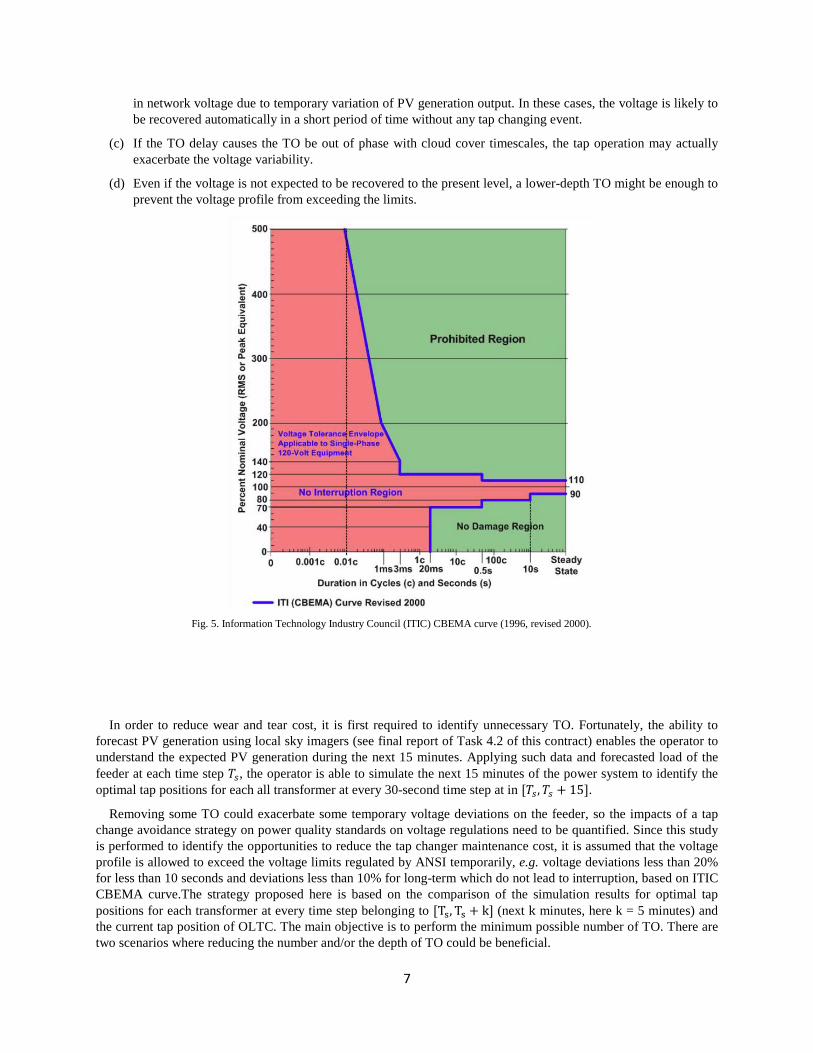
(a) A reasonably short voltage deviation is permitted while operating the distribution system. Fig. 5shows the Information Technology Information Council (ITIC) Computer and Business Equipment Manufacturers Association (CBEMA) Curve (revised 2000), where the interruption is presented as a function of voltage deviation and duration. For instance, voltage deviations less than 10% of nominal voltage do not cause any interruption, while 20% voltage deviation is only acceptable for a duration less than 10 seconds.

(b) As seen in Fig. 4, in such weather conditions, the TO is most likely performed in response to temporary change

7

in network voltage due to temporary variation of PV generation output. In these cases, the voltage is likely to be recovered automatically in a short period of time without any tap changing event.

(c) If the TO delay causes the TO be out of phase with cloud cover timescales, the tap operation may actually exacerbate the voltage variability.

(d) Even if the voltage is not expected to be recovered to the present level, a lower-depth TO might be enough to prevent the voltage profile from exceeding the limits.

Fig. 5. Information Technology Industry Council (ITIC) CBEMA curve (1996, revised 2000).

In order to reduce wear and tear cost, it is first required to identify unnecessary TO. Fortunately, the ability to forecast PV generation using local sky imagers (see final report of Task 4.2 of this contract) enables the operator to understand the expected PV generation during the next 15 minutes. Applying such data and forecasted load of the feeder at each time step 𝑇𝑇𝑠𝑠, the operator is able to simulate the next 15 minutes of the power system to identify the optimal tap positions for each all transformer at every 30-second time step at in [𝑇𝑇𝑠𝑠,𝑇𝑇𝑠𝑠 + 15].

Removing some TO could exacerbate some temporary voltage deviations on the feeder, so the impacts of a tap change avoidance strategy on power quality standards on voltage regulations need to be quantified. Since this study is performed to identify the opportunities to reduce the tap changer maintenance cost, it is assumed that the voltage profile is allowed to exceed the voltage limits regulated by ANSI temporarily, e.g. voltage deviations less than 20% for less than 10 seconds and deviations less than 10% for long-term which do not lead to interruption, based on ITIC CBEMA curve.The strategy proposed here is based on the comparison of the simulation results for optimal tap positions for each transformer at every time step belonging to [Ts, Ts + k] (next k minutes, here k = 5 minutes) and the current tap position of OLTC. The main objective is to perform the minimum possible number of TO. There are two scenarios where reducing the number and/or the depth of TO could be beneficial.

8

Observation 1: Tap reversal. Action: No TO

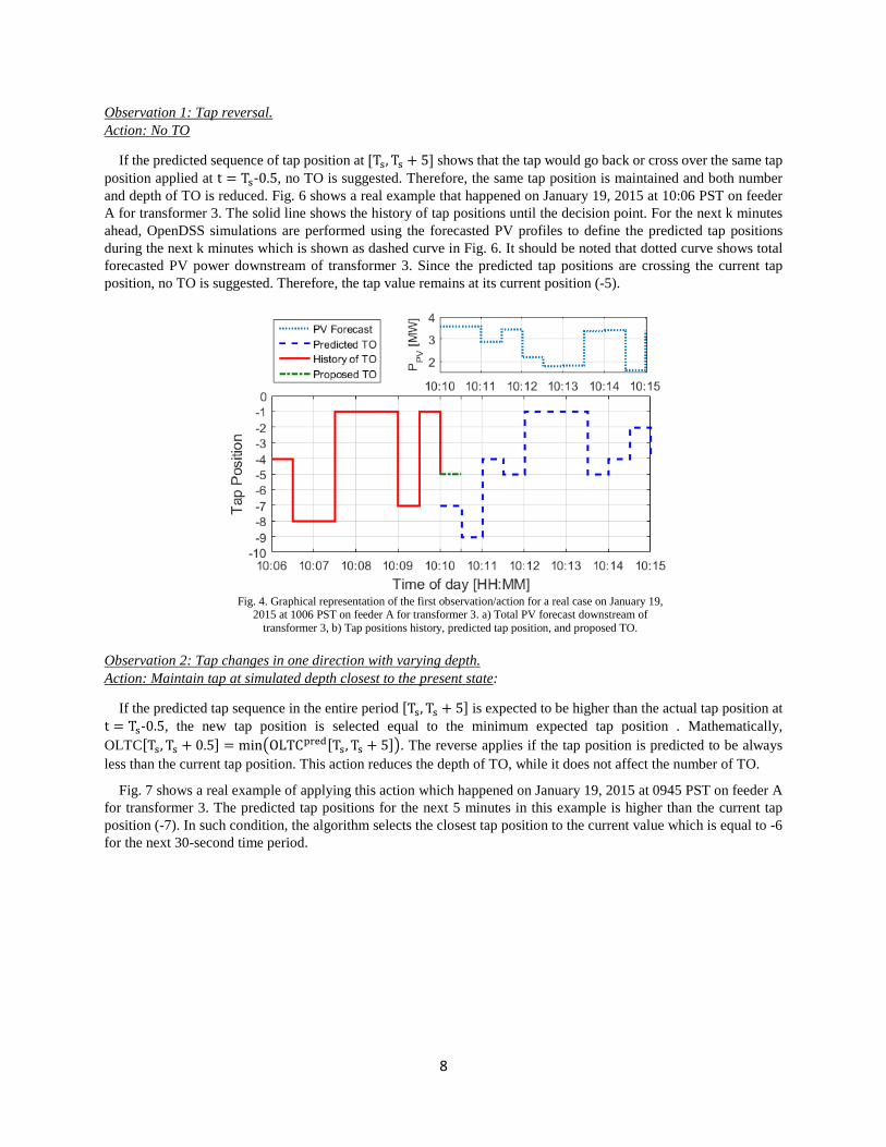
If the predicted sequence of tap position at [Ts, Ts + 5] shows that the tap would go back or cross over the same tap position applied at t = Ts-0.5, no TO is suggested. Therefore, the same tap position is maintained and both number and depth of TO is reduced. Fig. 6 shows a real example that happened on January 19, 2015 at 10:06 PST on feeder A for transformer 3. The solid line shows the history of tap positions until the decision point. For the next k minutes ahead, OpenDSS simulations are performed using the forecasted PV profiles to define the predicted tap positions during the next k minutes which is shown as dashed curve in Fig. 6. It should be noted that dotted curve shows total forecasted PV power downstream of transformer 3. Since the predicted tap positions are crossing the current tap position, no TO is suggested. Therefore, the tap value remains at its current position (-5).

Fig. 4. Graphical representation of the first observation/action for a real case on January 19,

2015 at 1006 PST on feeder A for transformer 3. a) Total PV forecast downstream of transformer 3, b) Tap positions history, predicted tap position, and proposed TO.

Observation 2: Tap changes in one direction with varying depth. Action: Maintain tap at simulated depth closest to the present state:

If the predicted tap sequence in the entire period [Ts, Ts + 5] is expected to be higher than the actual tap position at t = Ts-0.5, the new tap position is selected equal to the minimum expected tap position . Mathematically, OLTC[Ts, Ts + 0.5] = min�OLTCpred[Ts, Ts + 5]�. The reverse applies if the tap position is predicted to be always less than the current tap position. This action reduces the depth of TO, while it does not affect the number of TO.

Fig. 7 shows a real example of applying this action which happened on January 19, 2015 at 0945 PST on feeder A for transformer 3. The predicted tap positions for the next 5 minutes in this example is higher than the current tap position (-7). In such condition, the algorithm selects the closest tap position to the current value which is equal to -6 for the next 30-second time period.

9

Fig. 5. Graphical representation of the second observation/action via a real cases on January

19, 2015 at 0945 PST on feeder A for transformer 3. a) Total PV forecast downstream of transformer 3, b) Tap positions history, predicted tap position, and proposed TO.

Note that the decision for the TO is based on forecasted data with an inherent uncertainty. Therefore, two scenarios are examined: (i) Real forecasts from sky imagery are used. Forecast error may cause unnecessary tap changes and may cause less or more voltage violations. (ii) At each time step, the (future) now-cast data for the next 5 minutes, which is considered as the perfect forecast, is used in simulation instead. The difference between scenario (i) and (ii) shows the impacts of forecast error on the final results. Note that since decisions are not based on forecasts at a particular time but rather a forecast extremum (minimum value in the minimum depth rule) and forecast variability (no TO rule), the control scheme is robust against forecasts errors at individual time steps. For example, in Fig. 4 if a high tap was related to clear skies and a low tap to cloudy skies, then it would be sufficient to know that cloudy skies existed at least once at [Ts, Ts + 5]. From a forecasting standpoint, this level of accuracy is much easier to achieve than forecasting the cloud cover at each time step as phase errors in the forecast become irrelevant.

III. NUMERICAL RESULTS

To demonstrate the efficiency of the TO reduction method, it is tested on feeder A, as shown in Fig. 3, for 95 days between December 6, 2014 through March 15, 2015 for 100% PV penetration level. First, the base case simulations are carried out without applying the predictive tap changer control. This scenario which is exactly the same as the one simulated in Task 4.3 of this contract is noted as ‘No Control’ scenario in this report. Then, a 5-minute predictive tap changer control using the available forecast data at each time step is applied to observe its impact on both TO reduction and voltage quality. This scenario is noted as ‘Actual Forecast’ in this report. To evaluate the robustness of the actual forecast scenario against sky imager PV forecast error, the simulations are repeated by employing the actually recorded PV outputs and this scenario is noted as ‘Perfect Forecast’ in this report.

A. TO Reduction

Before examining the statistics of the simulation results, it is helpful to consider an example to show how different TO control scenarios reduce TO activities on OLTCs. Fig. 8 illustrates the one-hour window from 1000 through 1100 PST on January 19, 2015 (the same time period focused in ), with the tap position sequences of transformer 3 for different scenarios. In the “no control” scenario (base case), high variability of PV imposes 38 TO with a total depth of 135. Applying the perfect forecast scenario significantly reduces the number of TO to only one TO with depth of 2 taps, while the actual forecast scenario decreases the number and depth of TO to 9 and 17 respectively. Fig. 9 illustrates actual PV generation and forecasted PV curves at some time steps in the time period on January 19. Considering the curves depicted in Fig. 9, two major reasons are identified for the difference between the TO results of actual forecast and perfect forecast scenarios:

1- Initial condition error: At each time step, the current tap position in actual forecast scenario may differ from that in perfect forecast scenario. So even with a perfect forecast the results of two scenarios might be different

10

as prior forecast errors propagate into the current period. Nonetheless, it is expected that actual forecast scenario shows similar behavior to perfect forecast scenario when the PV forecast is accurate, as for example from 10:15 to 10:40 PST.

a. PV forecast error: Mismatch between the PV forecast and real PV output creates some differences between the TO results of actual and perfect forecast scenarios. For, example the forecast error at 10:05 and 10:10 (forecast clear versus actually partly cloudy) results in more TO in the actual forecast scenario. A similar situation happens at 10:50 when there is significant error in PV forecast data. It must be noted that the forecast error can result in more or less TO depending on the type of the error. If the PV forecast shows a clear sky while it is actually partly cloudy (more fluctuations in PV output than forecast,) more TO are performed in actual forecast scenario than perfect forecast, as shown in Fig. 9 and Fig. 8 at 10:05 to 10:10. On the other hand, less TO are performed in actual forecast compared to perfect forecast when a partly-cloudy PV forecast is performed for a clear sky.

Fig. 6. Tap position sequences of transformer 3 from 1000 to 1100 PST on Jan 19, 2015 for three different scenarios. Originally the number of TO was 38 and tap depth was 135. Using the actual forecast those are

reduced to 9 and 17. Using the perfect forecast, those are reduced to 1 and 2.

Fig. 7. Actual and forecasted total power output of the PV systems installed on feeder A at 100% penetration level from

1000 to 1100 PST on Jan 19, 2015. To avoid making the graph overly crowded, only the PV forecast issued every 5 minutes are shown. The forecast curves would be identical to the actual PV curve if the forecasts were perfect.

According to the 95-day simulation results, the maximum daily TO reduction and TO depth reduction are equal to 71.11% and 80.36% respectively, both occurring on February 7, 2015. On average, employing the tap reduction method decreases the daily number of TO from 461 to 247 TO per day, i.e., 46.5% reduction, while perfect forecasts reduce the number further to 251 TO/day resulting 45.5% reduction. The simulation results also show that the TO

11

depth can be reduced from an average of 761 taps per day to 334 taps per day (54.12% reduction) by actual forecast scenario while it could be decreased to 344 taps per day if the forecast is perfect. Table II presents more details about the performance of the control algorithms.

Table II: Impacts of the control strategies with perfect forecasts and actual forecasts on number and depth of TO. Average over 95 days Maximum within 95 days No

Control Actual

Forecast Perfect

Forecast No

Control Actual

Forecast Perfect

Forecast

TO number per day Value 461 247 251 1281 370 373 Reduction 46.5% 45.6% 71.1% 70.9%

TO depth per day Value 761 334 344 2561 503 545 Reduction 56.1% 54.7% 80.4% 78.7%

Fig. 10 illustrates the number and depth of TO by transformer in different control scenarios. Among the transformers connected to Fallbrook feeder, the 3rd and 7th transformers show the highest and lowest share of TO number and depth, respectively. These results are consistent with the fact that transformer 7 is the closest to the substation where the voltage is almost constant, while transformer 3 is the closest one to the end of the feeder and more prone to voltage excursions due to the large PV system. The simulation results show that both tap reduction scenarios with actual and perfect forecasts offer significant advantages and similar performance. The depth of TO of transformers 2 and 3 is reduced by 66% to about 50 and 60 TO/day which is much closer to the typical value for normal power transformers of 20 TO/day.

(a) (b)

Fig. 8. Impact of different control scenarios (no control, actual forecast, perfect forecast) on TO of transformers: a) average number of TO per day, b) average depth of TO per day

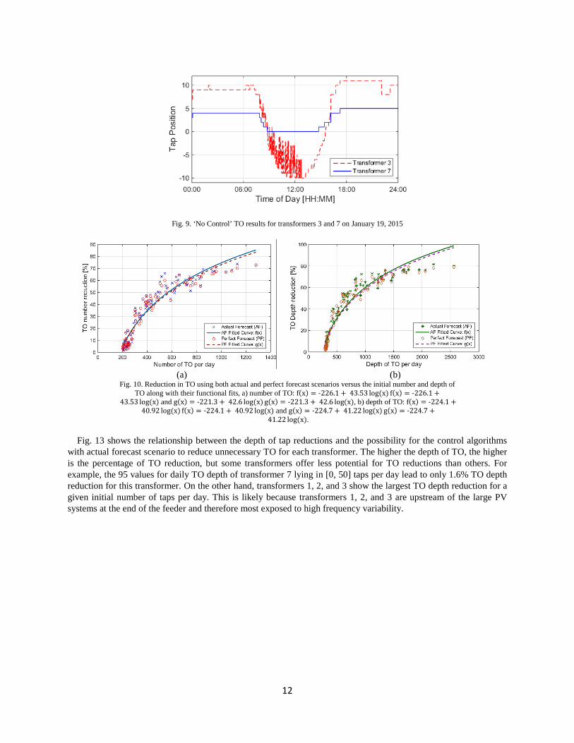
The possibility to reduce the number (depth) of TO strongly depends on the number (depth) of TO in the first place. For example, if there is only one TO in a 15-minute period, then neither rule will prevent it. For instance, the identical results for TO number/depth of transformer 7 for different control cases shown in Fig. 10 implies that none of the TO of this OLTC is unnecessary with respect to the two observations described in Section III and therefore cannot be eliminated. Fig. 11 shows the ‘No Control’ tap position sequences for transformers 3 and 7 on January 19, 2015. While the figure illustrates high number/depth of tap operations for transformer 3, the transformer 7 changes taps only as PV generation ramps up in the morning and down in the evening, but is not affected by high frequency PV variability.

Fig. 12 illustrates the reduction percentage versus the initial number/depth of TO per day in both actual and perfect forecast scenarios. It demonstrates that higher number and depth of TO coincide with higher reduction of number/depth of TO using both actual and perfect forecast scenarios. Fig. 12 implies that the high volume of TO indicative of partly-cloudy weather condition includes many unnecessary TO that could be eliminated by the predictive algorithms developed in this project. In other words, an increasing number of TO increases the likelihood that two or more TO exist in any given 15-minute period and are therefore potentially subject to elimination.

12

Fig. 9. ‘No Control’ TO results for transformers 3 and 7 on January 19, 2015

(a) (b)

Fig. 10. Reduction in TO using both actual and perfect forecast scenarios versus the initial number and depth of TO along with their functional fits, a) number of TO: f(x) = -226.1 + 43.53 log(x) f(x) = -226.1 +

43.53 log(x) and g(x) = -221.3 + 42.6 log(x) g(x) = -221.3 + 42.6 log(x), b) depth of TO: f(x) = -224.1 + 40.92 log(x) f(x) = -224.1 + 40.92 log(x) and g(x) = -224.7 + 41.22 log(x) g(x) = -224.7 +

41.22 log(x).

Fig. 13 shows the relationship between the depth of tap reductions and the possibility for the control algorithms with actual forecast scenario to reduce unnecessary TO for each transformer. The higher the depth of TO, the higher is the percentage of TO reduction, but some transformers offer less potential for TO reductions than others. For example, the 95 values for daily TO depth of transformer 7 lying in [0, 50] taps per day lead to only 1.6% TO depth reduction for this transformer. On the other hand, transformers 1, 2, and 3 show the largest TO depth reduction for a given initial number of taps per day. This is likely because transformers 1, 2, and 3 are upstream of the large PV systems at the end of the feeder and therefore most exposed to high frequency variability.

13

Fig. 11. Reduction in depth of TO using actual forecast scenario versus the initial number of TO per day for

individual transformers. For each transformers, the points with TO depth belonging to [50(k-1),50k][50(k-1),50k] are binned to the kthkth group with the indices xk = xk = 50k-2550k-25 and

ykyk equal to the average TO depth reductions of the points belonging to kthkth group.

B. Reduction of Capacitor Switching Events

To explore further opportunities to decrease the maintenance costs of the distribution system, similar algorithms are developed and applied to reduce the number of capacitor switching events. Both scenarios, with actual and perfect forecasts, are simulated on feeder A with 100% PV penetration for the same 95 days. Fig. 14 depicts the average number of capacitor switching events for all three control scenarios. As three capacitors are fixed capacitors and always connected to the grid, the number of switching events for them is zero. So, the focus of this part is on the first two capacitors. Although the capacitors 1 and 2 are switchable, the initial number of switching events is very low. As shown in Figs. 4 and 5, the control algorithm can reduce TO or capacitor switching events only if two changes occur within 5 minutes, which is unlikely with only 30 capacitor switching events per day. Similar to the results observed for transformer 7 in Fig. 10 and Fig. 13, the control algorithms cannot reduce the number of switching events significantly due to low number of capacitor switching events per day, as shown in Fig. 14.

(a) (b)

Fig. 12. Daily average data for capacitor switching events during 95 days of simulations through three different scenarios. a) Average number of capacitor switching events, b) Average depth of capacitor switching events

14

C. Voltage Analysis

Although the tap reduction control algorithms reduce the number/depth of TO, they may affect the voltage quality adversely. Therefore, it is crucial to investigate the voltage profile over the feeder in response to applying the proposed TO schedules. Since the control logic was applied in post-processing, the simulations had to be repeated with the OLTCs and capacitor switches locked on their specified values resulted from both actual and perfect forecast scenarios.

Fig. 15 shows the daily average maximum and minimum1 voltages that occurred on feeder A on 95 days of simulations through different control scenarios. As expected, the best voltage condition occurs when there is no tap reduction and the OLTC has the highest flexibility to perform the TO to counteract voltage excursions. The simulation results, however, demonstrate that the deviation of the voltage curves corresponding to actual and perfect forecast controls from the no-control scenario is minimal. Although the daily average maximum and minimum curves demonstrate insignificant impacts by control algorithms, daily maximum and minimum2 voltages are also of interest and may be more sensitive to the control scenario.

(a) (b)

Fig. 13. Daily average a) maximum and b) minimum voltages on 95 days for different control methods

Fig. 16 illustrates the maximum and minimum voltages that occurred on feeder A on 95 days of simulations for different control scenarios. These results show that while such voltage excursions are rare (see similar average maximum and minimum voltage in Fig. 15), the occasional forecast error can result in temporary large voltage deviations. On some days, even the perfect forecast does not avoid voltage deviations. The maximum voltage deviations which are caused by actual/perfect forecast scenarios are about 0.06 p.u. in Fig. 16a and 0.05 p.u in Fig. 16b, compared to the ‘No Control’ results. The maximum deviation of the voltage profiles from both maximum and minimum ANSI voltage limits on 95 days of simulations is about 0.07 p.u. for both TO control algorithms, but it must be noted that the maximum/minimum voltages in ‘no control’ case, were already outside the ANSI voltage limits.

1 At each time step, the maximum (minimum) voltage observed on the entire feeder is recorded. The average of these maximum (minimum) values during the daytime is referred to daily average maximum (minimum) voltage. 2 At each time step, the maximum (minimum) voltage observed on the entire feeder is recorded. The maximum (minimum) of these maximum (minimum) values during the daytime is referred to daily record maximum (minimum) voltage.

15

(a) (b)

Fig. 14. Daily record a) maximum and b) minimum voltages on 95 days for different control methods.

Having studied the daily record extremum voltages on the feeder, it is beneficial to investigate how frequent these voltage deviations happen. Fig. 17 shows two histogram of the extremum voltages during the 95 days of simulations. According to the simulation results shown in Fig. 17a, the maximum voltage values in the TO reduction scenarios exceed 1.1 p.u. about 0.2% of the simulation time, which is equal to 3 minutes per day. The results presented in Fig. 17b also demonstrate that the minimum voltages caused by actual and perfect forecast scenarios exceed the minimum threshold (0.95 p.u.) in just 5 and 8 time steps during the 95 days of simulations, i.e. 0.01% of the time.

(a) (b)

Fig. 15. Histogram of a) maximum and b) minimum voltages on 95 days for different control methods,

IV. CONCLUSIONS

A control strategy to reduce OLTC operations resulting from high PV penetration on distribution feeders was developed and applied. The strategy uses 5 minutes ahead solar forecast to derive future voltages states on the distribution feeder. Unnecessary TO are identified as those that are reversed within 5 minutes, likely because of temporary cloudy or clear conditions over adjacent PV systems.

On a feeder where TO were abundant at over 750 per day on average, the strategy resulted in the avoidance of 56% of the TO, which results in a significant savings in OLTC maintenance costs. Average extreme voltages were not affected by applying the TO reduction techniques. While the deviation of daily maximum/minimum voltage slightly increased on several days, a statistical analysis demonstrated that these deviations happened very rarely.

The strategy is most effective on partly cloudy days and on voltage regulators with a large number of TO, but the voltage quality might be adversely affected on these days. The fraction of avoided TO decreased substantially for less than 10 to 40 TO per day, depending on the voltage regulator.

REFERENCES [1] MR Group.The On-Load Tap-Changer for Maximum Switching Frequency – More Switching Operations without Needing Maintenance.

[Online]. Available: http://www.reinhausen.com/Portaldata/1/Resources/tc/products/oltc/vacutap_vr/F0220801_EN_Vacutap_VR1HD.pdf

16

[2] ABB. On-Load Tap-Changers, types UCC and UCD with motor-drive mechanism, type BUE – Installation and Commissioning Guide. . [Online]. 5. Available: https://library.e.abb.com/public/f95b7dc5c0bafaeec1256d3400231cda/1ZSE%205492-117%20en%20Rev%205.pdf

[3] S. Eftekharnejad, G. T. Heydt, and V. Vittal, “Optimal Generation Dispatch With High Penetration of Photovoltaic Generation,” IEEE Trans. Sustain. Energy, vol. 6, no. 3, pp. 1013–1020, Jul. 2015.

[4] S. Conti, S. Raiti, G. Tina, and U. Vagliasindi, “Study of the impact of PV generation on voltage profile in LV distribution networks,” in 2001 IEEE Porto Power Tech Proceedings (Cat. No.01EX502), 2001, vol. vol.4, p. 6.

[5] R. Tonkoski, D. Turcotte, and T. H. M. El-Fouly, “Impact of High PV Penetration on Voltage Profiles in Residential Neighborhoods,” IEEE Trans. Sustain. Energy, vol. 3, no. 3, pp. 518–527, Jul. 2012.

[6] N. Jayasekara and P. Wolfs, “Universities Power Engineering Conference (AUPEC), 2010 20th Australasian,” Universities Power Engineering Conference (AUPEC), 2010 20th Australasian. pp. 1–8, 2010.

[7] A. Hoke, R. Butler, J. Hambrick, and B. Kroposki, “Steady-State Analysis of Maximum Photovoltaic Penetration Levels on Typical Distribution Feeders,” IEEE Trans. Sustain. Energy, vol. 4, no. 2, pp. 350–357, Apr. 2013.

[8] J. E. Quiroz, M. J. Reno, and R. J. Broderick, “Time series simulation of voltage regulation device control modes,” in 2013 IEEE 39th Photovoltaic Specialists Conference (PVSC), 2013, pp. 1700–1705.

[9] R. J. Broderick, J. E. Quiroz, M. J. Reno, A. Ellis, J. Smith, and R. Dugan, "Time Series Power Flow Analysis for Distribution Connected PV Generation," Sandia National Laboratories SAND2012-2090, 2012.

[10] ABB, "Transformer protection RET670 v1.2. Application manual", Document ID: 1MRK 504 116-UEN, April 2011 [11] N. Daratha, B. Das, and J. Sharma, “Coordination Between OLTC and SVC for Voltage Regulation in Unbalanced Distribution System

Distributed Generation,” IEEE Trans. Power Syst., vol. 29, no. 1, pp. 289–299, Jan. 2014. [12] J. W. Smith, W. Sunderman, R. Dugan, and B. Seal, “Smart inverter volt/var control functions for high penetration of PV on distribution

systems,” in 2011 IEEE/PES Power Systems Conference and Exposition, 2011, pp. 1–6. [13] M. J. Reno, R. J. Broderick, and S. Grijalva, “Smart inverter capabilities for mitigating over-voltage on distribution systems with high

penetrations of PV,” in 2013 IEEE 39th Photovoltaic Specialists Conference (PVSC), 2013, pp. 3153–3158. [14] H. Yang, B. Kurtz, D. Nguyen, B. Urquhart, C. Chow, M. Ghonima, and J. Kleissl. (2014, May). Intra-hour forecasting with a total sky

imager at the UC San Diego energy testbed. Solar Energy. [Online]. 103, pp. 502-524. Available: http://dx.doi.org/10.1016/j.solener.2014.02.044