model predictive control approach for guidance of

INTERNATIONAL JOURNAL OF ROBUST AND NONLINEAR CONTROLInt. J. Robust. Nonlinear Control 2012; 22:1398–1427Published online 15 May 2012 in Wiley Online Library (wileyonlinelibrary.com). DOI: 10.1002/rnc.2827

Model Predictive Control approach for guidance of spacecraftrendezvous and proximity maneuvering‡

S. Di Cairano1, H. Park2 and I. Kolmanovsky2,*,†

1 Mechatronics, Mitsubishi Electric Research Laboratories�, Cambridge, MA, USA2Department of Aerospace Engineering, The University of Michigan, Ann Arbor, MI, USA

SUMMARY

Traditionally, rendezvous and proximity maneuvers have been performed using open-loop maneuverplanning techniques and ad hoc error corrections. In this paper, a Model Predictive Control (MPC) approachis applied to spacecraft rendezvous and proximity maneuvering problems in the orbital plane. We demon-strate that various constraints arising in these maneuvers can be effectively handled with the MPC approach.These include constraints on thrust magnitude, constraints on spacecraft positioning within Line-of-Sightcone while approaching the docking port on a target platform, and constraints on approach velocity to matchthe velocity of the docking port. The two cases of a nonrotating and a rotating (tumbling) platform are treatedseparately, and trajectories are evaluated in terms of maneuver time and fuel consumption. For the case whenthe platform is not rotating and the docking port position is fixed with respect to the chosen frame, an explicitoffline solution of the MPC optimization problem is shown to be possible; this explicit solution has a formof a piecewise affine control law suitable for online implementation without an on-board optimizer. In thecase of a fast rotating platform, it is, however, shown that the prediction of the platform rotation is necessaryto successfully accomplish the maneuvers and to reduce fuel consumption. Finally, the proposed approach isapplied to debris avoidance maneuvers with the debris in the spacecraft rendezvous path. The significance ofthis paper is in demonstrating that Model Predictive Control can be an effective feedback control approachto satisfy various maneuver requirements, reduce fuel consumption, and provide robustness to disturbances.Copyright © 2012 John Wiley & Sons, Ltd.

Received 2 August 2011; Revised 12 February 2012; Accepted 15 March 2012

KEY WORDS: spacecraft rendezvous and proximity maneuvering; spacecraft guidance; spacecraftdocking; constrained control; Model Predictive Control; debris avoidance

1. INTRODUCTION

Autonomous spacecraft rendezvous and proximity operations (RPO) are among the most importantand difficult elements of modern spacecraft missions. Examples of RPO maneuvers (see [1–3] andreferences therein) include a transport vehicle approach and docking to the International SpaceStation, a capture and recovery of a tumbling out-of-control satellite and a fly-by or avoidance of aspace object such as debris.

The requirements of RPO maneuvers invariably include the treatment of pointwise-in-time stateand control constraints. Examples include the thrust magnitude constraints, constraints on theapproaching spacecraft to maintain its position within a Line-of-Sight (LOS) cone emanating from

*Correspondence to: Ilya Kolmanovsky, Department of Aerospace Engineering, The University of Michigan, Ann Arbor,Michigan, USA.

†E-mail: [email protected]‡This manuscript is dedicated to Professor David W. Clarke of Oxford University, a gifted researcher and educator, anda role model for our community.�This research was not sponsored by Mitsubishi Electric or its subsidiaries.

Copyright © 2012 John Wiley & Sons, Ltd.

MPC APPROACH TO SPACECRAFT RENDEZVOUS AND PROXIMITY MANEUVERING 1399

the docking port on the target platform (see [4–7] and references therein), and constraints on theterminal translational velocity of the spacecraft to match the velocity of the docking port for soft-docking [8]. The docking port may exhibit complicated motion if the target spacecraft is rotating ortumbling out of control (see [5, 9]). Collisions with debris emerging on the spacecraft path must beavoided during the maneuvers. In addition to satisfying constraints, fuel consumption and maneuvertime must be minimized.

Spacecraft rendezvous control problems have received significant attention in the literature. See,for instance, [5, 7, 10–13] and references therein.

The main motivation for this paper is to demonstrate that Model Predictive Control (MPC) canbe an attractive feedback control approach for RPO maneuvering, which has traditionally beenperformed via open-loop “�v” sequencing (see e.g., [7]). In recent years, some approaches forspacecraft rendezvous and docking based on variants of the MPC framework have been proposed.In [14] the authors proposed an MPC strategy with variable horizon that requires the solution of amixed-integer linear program at every control cycle. Such a strategy is extended in [5] to generatefailure-safe trajectories. The variable horizon approach is further extended in [15] in the so-called “rubber band” MPC, where the MPC controller is designed by inverse optimality by usingtechniques similar to [16] with a horizon that first maintains a constant number of moves (as instandard MPC) and then decreases as in variable horizon MPC. An application of MPC to space-craft navigation in proximity of a space station is considered in [17], where an unconstrained MPCis proposed for guidance to the neighborhood of the space station, while the LOS between thestation and the spacecraft sensors is maintained by a constrained spacecraft attitude controller, and acontrol allocation scheme commands the thrusters. In a similar context, in [18], a receding horizoncontroller requiring the solutions of nonconvex quadratically constrained quadratic programs hasbeen proposed for passively safe proximity operations, where a statistical model of the uncertaintyis used for improving robustness with respect to position uncertainty.

The available spacecraft computing power may vary depending on the spacecraft, from that beingcomparable with a personal computer for high end spacecraft to being significantly more restrictedand even less than in automotive applications for low end spacecraft (nanosats or cubesats). Ineither cases, solutions that require lower computing effort are in demand for spacecraft applications.Any saved capacity can be used to deploy additional control, communications, and fault man-agement functions and/or reduce electric power consumption that is a very significant concern inthese applications.

Thus, motivated by considerations of computational feasibility for on-board implementation inorbiting spacecraft and differently from the previously mentioned literature, our approach to treat-ing RPO problems is based on utilizing to a maximum extent the LQ MPC framework with constanthorizon, real-valued optimization variables, and dynamically reconfigurable linear constraints. TheMPC cost function is specified with stage and terminal costs defined on the basis of Lyapunov sta-bility considerations. The online computations in the case of such an LQ MPC reduce to solvinga quadratic program subject to linear constraints (see [19]), and in many cases, such as whenapproaching a nonrotating platform, this problem can be solved explicitly offline by using theparametric quadratic programming techniques developed in [20, 21]. With such an explicit MPCapproach, the solution can simply be stored in the form of piecewise affine feedback law for onlineimplementation. Preliminary results using this approach have been discussed by the authors in[22–24] and are here analyzed with more details and using problem specifications closer to theones of real spacecraft applications.

For the general case of a rotating platform, the approach developed in this paper aims at overcom-ing a limitation of the standard MPC approach, namely the assumption of completely time-invariantplant and prediction model. Although not yet fully adaptive as a (constrained) Generalized Pre-dictive Control [25, 26], where the entire plant model and optimal controller are identified online,the proposed MPC with dynamically reconfigurable constraints reduces the gap between MPC andGeneralized Predictive Control, by allowing some degrees of adaption to modified externalconditions (i.e., different docking port position and orientation in the considered application).

To illustrate our approach in detail, in the paper, we consider spacecraft maneuvering in closeproximity to a disk-shaped target platform orbiting the Earth along a circular orbital track. Our

Copyright © 2012 John Wiley & Sons, Ltd. Int. J. Robust. Nonlinear Control 2012; 22:1398–1427DOI: 10.1002/rnc

1400 S. DI CAIRANO, H. PARK AND I. KOLMANOVSKY

treatment is based on the assumption of point mass spacecraft, circular orbit, and in-orbital planemotion. These assumptions are reasonable for many maneuvers and can be relaxed. We first con-sider a scenario when the platform is nonrotating relative to its center of mass and then a scenariowhen the platform is rotating with known constant angular velocity relative to its center of mass. AClohessy–Wiltshire–Hill (CWH) relative motion model is used by the MPC controller for repeatedprediction and constrained optimization of spacecraft motion in response to the thrust sequence.Constraints on LOS cone positioning, terminal velocity for soft-docking, thrust magnitude, anddebris avoidance are dynamically reconfigured and approximated by linear constraints, which arethen enforced by the MPC controller.

The paper is organized as follows. In Section 2, we discuss spacecraft and target platformequations of motion, as well as various modeling details. The constraints in the RPO problemand their dynamic reconfiguration by linear constraints are the subject of Section 3. In Section 4,we develop MPC controllers for the cases without and with prediction of the platform motion. InSection 5, we examine the simulated trajectories for the case of a nonrotating platform, and we ana-lyze the impact of the weights in the MPC cost function on fuel consumption-related metrics andtime-to-dock. The robustness of the MPC controller is demonstrated by simulating the spacecraftmotion as affected by unmeasured disturbances and comparing the closed-loop trajectories with theopen-loop trajectories. The disturbances can occur because of air drag on a Low Earth orbit or errorsin generating spacecraft thrust. An explicit MPC controller is also constructed in this section. Fora rotating target platform, which is the case considered in Section 6, the trajectories, the fuel con-sumption, and the time-to-dock are compared for the implementation of the MPC controller withthe prediction of the target’s platform motion and without such a prediction. Finally, in Section 7,we demonstrate that our approach can be applied to the debris avoidance maneuvers. Concludingremarks are made at the end of the paper, in Section 8.

The main contributions of the paper are summarized as follows. First, we demonstrate that variousconstraints in the RPO problem can be handled using an LQ MPC approach coupled with dynamicreconfiguration of the (linear) constraints. This approach is feasible for implementation on-board ofthe spacecraft either through an online solution using a quadratic programming solver or in the caseof nonrotating platform using an explicit MPC approach. Second, we demonstrate the capability ofthe spacecraft, controlled with MPC, to perform an approach of either a nonrotating platform or ofa rotating platform and avoid debris on the spacecraft path. Fly-over imaging maneuvers involvecontrolling spacecraft motion on a periodic orbit around another object and can be handled usingtechniques developed here for approaching a rotating platform. Third, we demonstrate the robust-ness to unmeasured disturbances through the mechanism of systematic feedback corrections withMPC. Fourth, we demonstrate a direct connection between weights in the MPC cost function andfuel consumption and time-to-dock maneuver attributes. These results suggest that the currentlyemployed open-loop guidance schemes coupled with ad hoc error correction procedures can bereplaced in the future by a closed-loop guidance based on MPC that systematically compensates fordisturbances and enforces constraints.

2. EQUATIONS OF MOTION

We consider autonomous rendezvous and docking maneuvers between a target platform and a space-craft. The target platform is assumed to have a disk shape of radius rp (m). If the platform does nothave disk shape to begin with or for fly-over maneuvers, the platform can be over-bounded by a diskof a sufficiently large radius, see Figure 1. The center of mass of the platform is on a circular orbitaround the Earth, and the orbital radius is R0 (m), see Figure 2. A docking port is located on theplatform surface. The platform rotates at a constant angular velocity !p > 0 (rad/s) around its centerof mass. The spacecraft is represented by a point mass, and it has to approach the target platformfor docking to the port.

We confine the motion of the target and of the spacecraft to the orbital x � y plane, where y cor-responds to the along the orbital track direction and x corresponds to the radial direction along theradius-vector from the center of the Earth to the target platform. The disturbances, for instance,because of air drag, solar pressure, and nonspherical gravity perturbation (J2) effects [27], are



Figure 1. Schematics of spacecraft and target platform with Line-of-Sight cone.

Figure 2. Relative frame centered at the target platform and relative coordinates.

neglected in the model formulation because their effects during the short time of the maneuvercan be compensated by the MPC feedback, as we will show later via simulations.

The treatment of planar spacecraft motion is consistent with requirements of typical rendezvousand docking maneuvers [7]. The out-of-plane relative dynamics are decoupled from the planardynamics and are stable, and hence are neglected, here.

The spacecraft translational motion is actuated by thrusters. We assume that thrusters can beoperated to generate prescribed propulsive forces in x and y directions and that the thrust mag-nitude is limited. The prescribed thrust forces can be physically realized by control allocation toappropriate thruster on–off times, see [7, 17]. For a single main thruster spacecraft configuration,



we assume that the spacecraft orientation is changed appropriately by the attitude control system torealize the prescribed thrust vector. The MPC feedback can be relied upon to compensate for thrustvector direction and magnitude errors, as it will be shown later in simulations.

To express the motion of the spacecraft relative to the target platform, we use the CWH equations[10, 27]. Because the target platform is in a circular orbit around the Earth of radius R0 (m), theorbital rate is n D

q�

R30

(rad/s), where � (m3/s2) is the gravitational constant of the Earth. The

reference Hill’s frame is located at the target platform center of mass; hence, it rotates with orbitalrate n with respect to the inertial reference frame that is located at the center of the Earth. The posi-tion vector to the target’s center of mass from the center of the Earth is expressed as ER0 DR0O{. Therelative position vector of the spacecraft with respect to the platform is expressed as ıEr D ıxO{Cıy O| ,where ıx, ıy (m) are the components of the position vector of the spacecraft relative to the platformcenter. The position vector of the spacecraft with respect to the center of the Earth is thus given byER D ER0 C ıEr D .R0 C ıx/O{ C ıy O| . The equations of motion for the spacecraft are nonlinear and

can be expressed in vector form as

RERD��ER

R3C

1

mcEF , (1)

where EF denotes the vector of forces applied to the spacecraft and mc (kg) is the mass of thespacecraft. Given that RD

p.R0C ıx/2C ıy2Œm�, we obtain

RERD�ı Rx � 2nı Py � n2.R0C ıx/

�O{ C

�ı Ry C 2nı Px � n2ıy

�O| .

For ır << R, the CWH equations [10, 27] approximate the relative motion dynamics as

ı Rx � 3n2ıx � 2nı Py DFx

mcD ux ,

ı Ry C 2nı Px DFy

mcD uy ,

(2)

where ux ,uy (m/s2) are acceleration components of the spacecraft in x and y directions, inducedby the thrust forces Fx ,Fy (N), respectively. The spacecraft accelerations are subsequently treatedas control signals as it is common in these applications [7].

Model (2) can be formulated as

PX D AX CBU , (3)

where X 2R4 is the state vector, U 2R2 is the control vector, and

X D

0B@ıx

ıy

ı Pxı Py

1CA , AD

0BB@

0 0 1 0

0 0 0 1

3n2 0 0 2n

0 0 �2n 0

1CCA , B D

0B@0 0

0 0

1 0

0 1

1CA , U D

�uxuy

�.

For the development of the MPC controller, continuous-time spacecraft model (3) is discretizedin time with sampling period Ts (s) leading to the discrete-time model

X.kC 1/D AdX.k/CBdU.k/, (4)

where X.k/ 2 R4 and U.k/ 2 R2 denote, respectively, the state and input vectors at the samplinginstant k 2 Z0C.

The coordinates of the docking port in Hill’s frame at time instant k are associated to the statevariables rx.k/, ry.k/ (m) and have dynamics

rx.kC 1/D cos.!pTs/rx.k/� sin.!pTs/ry.k/,

ry.kC 1/D sin.!pTs/rx.k/C cos.!pTs/ry.k/,(5)



where !p (rad/s) is the angular velocity of the platform about its center of mass. If the targetplatform is not rotating, then !p D 0 and rx.k C 1/ D rx.k/, ry.k C 1/ D ry.k/. In the rotat-ing platform case, (5) enables to use MPC for docking to a moving port. The relative coordinates ofthe spacecraft with respect to the docking port are defined as

�x.kC 1/D ıx.k/� rx.k/,

�y.kC 1/D ıy.k/� ry.k/.(6)

The state vector, augmented with the position of the docking port and the relative coordinatesfrom (6), has the following form:

NX D�ıx ıy ı Px ı Py rx ry �x �y

�T.

From (4)–(6), we can formulate the system model as

NX.kC 1/D NA NX.k/C NB NU .k/, (7)

with appropriately defined NA, NB , and NU D ŒU T s�T , where s is an auxiliary slack variable used inthe definition of the constraints, as explained next.

3. CONSTRAINT MODELING AND DYNAMIC RECONFIGURATION

For computational efficiency reasons, we base our approach to RPO maneuvering on the appli-cation of an LQ MPC with linear inequality constraints. Various constraints in the RPO controlproblem and the procedure to handle them by dynamically reconfigurable linear constraints arenow discussed.

3.1. Thrust constraints

For a single thruster spacecraft, the constraint on the maximum thrust magnitude has the followingform:

u2x C u2y 6 u2max. (8)

This constraint is nonlinear, but in the LQ MPC, we can only enforce linear input constraints.By constraining

�umaxp26 ux.k/6

umaxp2

, �umaxp26 uy.k/6

umaxp2

, (9)

constraint (8) can be conservatively enforced. To avoid unnecessary control authority reduction, weimpose the thrust magnitude constraints in the form

� umax 6 ux.k/6 umax, � umax 6 uy.k/6 umax, (10)

and if ux.k/2 C uy.k/2 > u2max occurs for some k, we modify the computed ux.k/ and uy.k/ bydirectionality preserving scaling [7],

u0x.k/Dux.k/p

ux.k/2C uy.k/2umax, u0y.k/D

uy.k/pux.k/2C uy.k/2

umax. (11)

Remark 1The approach mentioned earlier can be generalized to enforcing constraint

� N�umax 6 ux.k/6 N�umax, � N�umax 6 uy.k/6 N�umax, (12)

where N� 2 Œ1=p2, 1� is a parameter, chosen offline, that trades off conservativeness of the constraints

and reliability of the trajectory prediction. In fact, for N� D 1=p2, (12) reduces to (9), which is more

conservative than (10), hence, limiting the performance, but it ensures that the acceleration for the



planned trajectory can always be achieved. Instead for N� D 1, (12) reduces to (10), which is lessconservative, yet it may occasionally happen that the acceleration for the planned trajectory cannotbe actually achieved. For N� 2 .1=

p2, 1/, the intermediate trade-offs are obtained.

Remark 2Constraint (8) is a convex quadratic constraint. Hence, if added to the quadratic program that isgenerated by LQ MPC, it results in a convex Quadratically Constrained Quadratic Program (QCQP).The QCQPs are indeed more complex than linearly constrained QPs, but specific algorithms thatexploit their structure to provide faster solution are becoming available [28]. Alternatively, theproblem can be formulated and solved as a Second Order Cone Program [29], for which the solu-tion usually requires more time and resources than what is typically available for this application.Because here we focus on obtaining a controller that can execute even with limited computationalresources, we choose to apply approximation (12), solve the resulting QP, and perform scaling (11),if needed.

3.2. Line-of-Sight constraints

The LOS constraints confine the spacecraft to the intersection of the LOS cone, with vertex movedslightly inside the platform and a half-plane. See lines a, b, and c in Figure 3. Let � denote the halfof the LOS cone angle, and let rtolŒm� denote the distance by which the vertex of LOS cone is movedinside the platform. The value rtol > 0, which is chosen offline, slightly relaxes the LOS constraintsto mitigate ill conditioning of the problem caused by the LOS constraints, corresponding to a and b,becoming borderline feasible as the spacecraft approaches the docking port. The constraint corre-sponding to the half-plane c, defined by a tangent line to the platform at the position of the dockingport, ensures that collisions of the spacecraft with the target platform are avoided with the relaxedcone constraints.

The LOS constraints are mathematically defined by8<ˆ:

a W sin.'.k/C�/.rp�rtol/ sin� ıx.k/�

cos.'.k/C�/.rp�rtol/ sin� ıy.k/> 1,

b W � sin.'.k/��/.rp�rtol/ sin� ıx.k/C

cos.'.k/��/.rp�rtol/ sin� ıy.k/> 1,

c W cos'.k/rp sin� ıx.k/C

sin'.k/rp sin� ıy.k/> 1,

(13)

where '.k/ is the angle between the platform docking port and the x-axis at the time instant k.

Figure 3. Geometric representation of the Line-of-Sight constraints.



For the case where the platform is not rotating and '.k/ is constant, that is, '.k/ D ', the LOSconstraints are linear inequalities in ıx.k/ and ıy.k/. For the case where the platform rotates, thatis, '.k/ changes in time, we will consider and compare two approaches for the treatment of LOSconstraints (13) over the prediction horizon of the MPC problem. In the first approach, '.k/ isassumed to remain constant over the prediction horizon, and the constraints remain frozen. In thesecond approach (see Section 4.2), we will approximately predict the changes in the LOS constraintbecause of the platform rotation.

3.3. Soft-docking constraint

The soft-docking constraint ensures that the relative velocity of the spacecraft, once it approachesthe docking port, is close to the docking port velocity. This ensures that the spacecraft can followthe port and avoid excessive mechanical shock when docking occurs.

Because the soft-docking constraint is a terminal constraint, to handle it by using the conventionalMPC formulation, we consider a related pointwise-in-time constraint, requiring that the 1-norm ofthe spacecraft velocity relative to the docking port is bounded by an affine function of the 1-normof the distance of the spacecraft relative to the docking port. A similar approach was used in ourprevious work [30] to handle the soft-landing constraints for an electromagnetic actuator.

In this paper we use the notation a.j jk/ to indicate the value of a variable a predicted j

steps ahead from step k. Let �x.j jk/, �y.j jk/ be the predicted values of the spacecraft positionin x and y directions relative to the docking port j steps ahead, given that k is the currenttime instant at which the computations are performed. Similarly, let the predicted relative veloc-ities be denoted by ı Px.j jk/ and ı Py.j jk/ (m/s). The docking port velocities can be predicted byvpx .j jk/ D �!pry.j jk/ and vpy .j jk/ D !prx.j jk/, which we use to enforce over the MPCprediction horizon the constraint

j�x.j jk/j C j�y.j jk/j> �¹jı Px.j jk/� vpx .j jk/j C jı Py.j jk/� vpy .j jk/j � s.j jk/º � ˇ. (14)

Here, � > 0 and ˇ > 0 are constant parameters that define the shape of the feasible set in theposition-velocity space. The variable s.j jk/ is a slack variable that was introduced as a componentof NU in (7), and is used to avoid infeasibility of constraint (14).

To handle constraint (14), which is pointwise-in-time but still ‘mildly’ nonlinear, we replace it bya related linear constraint on the basis of the assumption that over the prediction horizon, the signsof �x.j jk/, �y.j jk/, ı Px.j jk/ � vpx .j jk/ and ı Py.j jk/ � vpy .j jk/ do not change. This leads to adynamically reconfigurable constraint of the form

sgn.ıx.k//.�x.j jk//C sgn.ıy.k//.�y.j jk//> �¹sgn.ı Px.k/� vpx .k//.ı Px.j jk/� vpx .j jk//

C sgn.ı Py.k/� vpy .k//.ı Py.j jk/� vpy .j jk//� s.j jk/º � ˇ, (15)

where sgn.�/ indicates the well-known sign function. The mismatch between the predicted trajectorybased on this simplifying assumption and the actual spacecraft trajectory is compensated becauseof MPC recomputing the solution at every time instant and updating the constraint representation inreal-time.

With a limited loss of performance, constraint (15) can be further simplified to

�.k/> �¹sgn.ı Px.k/� vpx .k//.ı Px.j jk/� vpx .j jk//

C sgn.ı Py.k/� vpy .k//.ı Py.j jk/� vpy .j jk//� s.j jk/º � ˇ, (16)

where

�.k/�D jıx.k/� rx.k/j C jıy.k/� ry.k/j

D j�x.k/j C j�y.k/j.(17)

The approach taken here to approximately handle the soft-docking constraint (and relatedapproach for debris avoidance in Section 7) simplifies the optimization problem to a level thatenables its treatment by computationally effective, conventional MPC techniques based on linear



models with linear constraints. Our subsequent simulation results indicate that this approach doesnot compromise the response properties and enforces satisfactorily the constraints.

4. MODEL PREDICTIVE CONTROLLER DESIGN

With the dynamic model and constraints defined in Section 3, we design the MPC controller for thecases of nonrotating and rotating platforms.

To define the cost function for the MPC controller, we first compute the value function of theinfinite horizon unconstrained LQ problem for stabilizing the relative position and velocity of thespacecraft to the origin, that is,

minU.�/

J D

1XkD0

X.k/TQX.k/CU.k/TRU.k/, (18)

where

QD

0B@Q11 0 0 0

0 Q22 0 0

0 0 Q33 0

0 0 0 Q44

1CAD

�Q1 02�2

02�2 Q2

�, RD

�R11 R12R21 R22

�,

U.�/ D ¹U.0/,U.1/, : : :º and 0n�m denotes an n � m zero matrix. In (18), Q is a positive-definite state weighting matrix, and R is a positive-definite control weighting matrix. Let P denotethe solution of the Riccati equation for solving problem (18) and K the corresponding LQRfeedback gain,

P D

0B@P11 P12 P13 P14P21 P22 P23 P24P31 P32 P33 P34P41 P42 P43 P44

1CAD

�P1 P2P3 P4

�, K D

�K11 K12 K13 K14K21 K22 K23 K24

�,

so that the value function is .X.0//DX.0/TPX.0/ for the LQ problem. We use P in the terminalcost of the MPC problem, consistently with the classical MPC theory (see [16,31,32]) as a stabilityenforcing mechanism.

4.1. Model Predictive Controller without prediction of platform motion

For the case of an MPC controller that does not use the prediction of the platform motion over thehorizon, the prediction model is based on (7) and (13) with !p D 0 and '.k/D '. We can expressthe prediction model in the form

NX.j C 1jk/D NA NX.j jk/C NB NU .j jk/, (19a)

NY .j jk/D NC NX.j jk/C ND NU.j jk/, (19b)

where (19b) represents the constrained output because of (7) and (14). These output constraints areimposed as

NY .j jk/> NYmin.k/, (20)

where NYmin.k/ D�1 1 1 �ˇ � �.k/

�T. The matrices NA, NB , NC , and ND in (19) are expressed

as

NAD

0@ Ad 04�4

02�2 02�2 02�2I 02�2 �I 02�2

1A , NB D

�Bd 04�1

04�2 04�1

�,



NC D

0BB@NC11 NC12 0 0 0 0 0 0NC21 NC22 0 0 0 0 0 0NC31 NC32 0 0 0 0 0 0

0 0 NC43 NC44 NC45 NC46 0 0

1CCA , (21)

ND D

�03�2 03�101�2 �

�,

where

D

�cos.!pTs/ � sin.!pTs/sin.!pTs/ cos.!pTs/

�, I D

�1 0

0 1

�,

and by assuming '.j jk/D '.k/D ',

NC11 Dsin.' C �/

.rp � rtol/ sin �, NC12 D�

cos.' C �/

.rp � rtol/ sin �, NC21 D�

sin.' � �/

.rp � rtol/ sin �,

NC22 Dcos.' � �/

.rp � rtol/ sin �, NC31 D

cos'

rp sin �, NC32 D

sin'

rp sin �.

Here, NC11, NC12, NC21, NC22, NC31, and NC32 are used to represent LOS constraints (13). The ele-ments NC43, NC44, NC45, and NC46 of NC are used to model (16), which approximates soft-dockingconstraint (14). Note that if ı Px.k/ � vpx .k/ > 0, then NC43 D ��, NC46 D �!p; otherwise,NC43 D �, NC46 D ��!p . If ı Py.k/ � vpy .k/ > 0, then NC44 D ��, NC45 D ��!p; otherwise,NC44 D �, NC45 D �!p .

At every time instant k, the MPC controller determines the control action on the basis of thesolution of the following optimization problem

minNU.k/

NX.NJ jk/T NP NX.NJ jk/C

NJ�1XjD0

NX.j jk/T NQ NX.j jk/C NU.j jk/T NR NU.j jk/, (22a)

s.t. NX.j C 1jk/D NA NX.j jk/C NB NU.j jk/, (22b)

NY .j jk/D NC NX.j jk/C ND NU .j jk/, (22c)

NX.0jk/D NX.k/, (22d)NU.j jk/D NK NX.j jk/, j DNU C 1, : : : ,NJ � 1, (22e)NY .j jk/> NYmin.k/, j D 0, : : : ,NC , (22f)NU.j jk/> NUmin, j D 0, : : : ,NU , (22g)NU.j jk/6 NUmax, j D 0, : : : ,NU , (22h)

where NU.k/ D ¹ NU.0jk/, : : : , NU .NU jk/º, NJ denotes the prediction horizon, NU denotes thecontrol horizon, and NC denotes the constraint horizon. Smaller values of NU and Nc tend toreduce the complexity of optimal control problem (22) and hence computational requirement of theplatform where the MPC controller is executed. The input constraints in (22) are defined by (10).The matrices NP , NQ, NR, and NK are constructed from Q and R in (18) and the solution, P , of theRiccati equation and the LQR gain NK for (18) as

NP D

0B@

02�2 02�2 02�2 02�202�2 P4 02�2 P302�2 02�2 02�2 02�202�2 P2 02�2 P1

1CA , NQD

0B@

02�2 02�2 02�2 02�202�2 Q2 02�2 02�202�2 02�2 02�2 02�202�2 02�2 02�2 Q1

1CA ,

NRD

�R 02�1

01�2 �

�, NK D

�02�2 K13 K14 02�2 K11 K1202�2 K23 K24 02�2 K21 K22

�.

In (22), � > 0 is a large weight on the slack variable causing this to be zero whenever feasible.



At every control cycle, from the measured/estimated state NX.k/, the MPC controller solves (22)with respect to the finite sequence of control actions, NU.k/, and applies the first element of theoptimal sequence NU�.k/ to the plant, NU .k/ D NU �.0jk/. The MPC feedback law is defined implic-itly as the solution of constrained optimization problem (22); however, because of the structureof (22), this feedback law is a static (nonlinear) function of the current state, NU .k/D NUMPC. NX.k//.

4.2. Model Predictive Controller with prediction of platform motion

Even if the constraints in (22) change with time, as the initial state of the finite horizon optimalcontrol problem NX changes, the bounds are assumed constant in prediction. In this section, we pro-pose a method to incorporate a prediction of LOS constraints (13) changes because of the rotation ofthe docking port for the MPC optimization problem. To continue exploiting an LQ MPC framework,we employ the approximations on the basis of the Taylor series expansion

'.j jk/' '.k/C P'.k/jTs D '.k/C N'.j , k,Ts/, (23)

sin.'.j jk/C �/' sin.'.k/C �/C cos.'.k/C �/ N'.j , k,Ts/,

cos.'.j jk/C �/' cos.'.k/C �/� sin.'.k/C �/ N'.j , k,Ts/,(24)

where k denotes the current time instant and j 2 Z0C is a future time instant with respect to k. Bysubstituting (23) and (24) into the LOS constraints (13), we can obtain the following LOS constraintsfor prediction of the platform motion:8<

:a0 W L1ıx.j jk/�L2ıy.j jk/C ¹L2ıx.k/CL1ıy.k/º.'.j jk/� '.k//> 1,

b0 W �L3ıx.j jk/CL4ıy.j jk/� ¹L4ıx.k/CL3ıy.k/º.'.j jk/� '.k//> 1,

c0 W L5ıx.j jk/CL6ıy.j jk/� ¹L6ıx.k/CL5ıy.k/º.'.j jk/� '.k//> 1,

(25)

where

L1 Dsin.'.k/C �/

.rp � rtol/ sin �, L2 D

cos.'.k/C �/


sin.'.k/� �/

.rp � rtol/ sin �,

L4 Dcos.'.k/� �/


cos.'.k//

rp sin �, L6 D

sin.'.k//

rp sin �.

In addition, to predict the future position of the LOS cone, we introduce the auxiliary state vector,

Z.j jk/D

�´1´2

�D

�'.j C 1jk/'.j jk/

�D

�'.j jk/C!pTs

'.j jk/

�, (26)

with dynamics defined by

Z.j C 1jk/D

�2 �11 0

�Z.j jk/D‚Z.j jk/. (27)

Considering (7), (25), and (27), the augmented prediction model has state vector

QX D�ıx ıy ı Px ı Py rx ry �x �y ´1 ´2

�T(28)

and dynamics formulated as a linear system subject to time-varying constraints

QX.j C 1jk/D QA QX.j jk/C QB QU .j jk/, (29a)

QY .j jk/D QC QX.j jk/C QD QU.j jk/, (29b)

where

QAD

�NA 08�2

02�8 ‚

�, QB D

�NB

02�3

�, QD D ND, QU D NU ,



QC D

0BB@NC11 NC12 0 0 0 0 0 0 0 QCLOS1NC21 NC22 0 0 0 0 0 0 0 QCLOS2NC31 NC32 0 0 0 0 0 0 0 QCLOS3

0 0 NC43 NC44 NC45 NC46 0 0 0 0

1CCA ,

QCLOS1 D L2ıx.k/CL1ıy.k/,

QCLOS2 D�L4ıx.k/�L3ıy.k/,

QCLOS3 D�L6ıx.k/�L5ıy.k/,

so that we have the auxiliary state vector and terms for the LOS constraints in the new model.The output constraints (cf. (20)) are

QY .j jk/> QYmin.k/, QYmin.k/D NYmin.k/. (30)

Thus, for the case where prediction of the port motion is performed, the MPC optimal controlproblem is formulated from (28)–(30) as

minQU.k/

QX.NJ jk/T QP QX.NJ jk/C

NJ�1XjD0

QX.j jk/T QQ QX.j jk/C QU.j jk/T QR QU.j jk/,

(31a)

s.t. QX.j C 1jk/D QA QX.j jk/C QB QU .j jk/, (31b)

QY .j jk/D QC QX.j jk/C QD QU .j jk/, (31c)

QX.0jk/D QX.k/, (31d)

QU .j jk/D QK QX.j jk/, j DNU C 1, : : : ,NJ � 1, (31e)

QY .j jk/> QYmin.k/, j D 0, : : : ,NC , (31f)

QU .j jk/> QUmin, j D 0, : : : ,NU , (31g)

QU .j jk/6 QUmax, j D 0, : : : ,NU , (31h)

where QU.k/D®QU .0jk/, : : : , QU .NU jk/

¯,

QP D

�NP 08�2

02�8 02�2

�, QQD

�NQ 08�2

02�8 02�2

�, QRD NR, QK D

�NK 02�2

�,

and the input constraints in (31) are defined by (10).

5. SIMULATED APPROACH OF A NONROTATING PLATFORM

In the simulations, we have used the following parameters representative of spacecraft maneuveringin close proximity of a nonrotating target platform: the radius of the target rp is 2.5m, the half angleof the LOS cone � is 10 deg, the tolerance rtol is 0.5 m, and the orbital rate n is 1.107� 10�3 rad/s(corresponding to the orbit of 500 km above the Earth). The controller sampling period is Ts D 0.5 s.The total maneuver simulation time is 100 s. In (14), �D 1, and ˇ D 2.5

10. The slack variable weight

is set as �D 1010. The weighting matrices are chosen in the form

QD 3� 103�102I 02�202�2 I

�, RD 102I .

The value of R was subsequently modified to study the sensitivity of fuel consumption andtime-to-dock. In the simulations, we use umax D 0.2 m/s2 for the input constraints.

For all simulations, the prediction horizon of the MPC problem was set asNJ D 40, the constrainthorizon for both input and output constraints was set as NC D 5, and the control horizon was set asNU D 5. These values were determined by tuning closed-loop response by using simulations.



5.1. Radial approach

In the radial approach, the spacecraft approaches the platform along the radial line from the centerof the Earth to the center of the target. To simulate the radial approach, we choose the initial locationfor the spacecraft as .ıx0, ıy0/ D .100,�10/ (m), which is in the range of admissible initial con-ditions for RPO maneuvers and the initial position of the docking port as .rx0, ry0/D .2.5, 0/ (m).The closed-loop responses are shown in Figure 4. In this and other plots of spacecraft trajectory onthe x�y plane, the LOS constraints are shown by red dashed lines. The soft-docking, the LOS cone,and thrust magnitude constraints are enforced by the MPC controller, and the spacecraft successfullycompletes the maneuver.

5.2. In-track approach

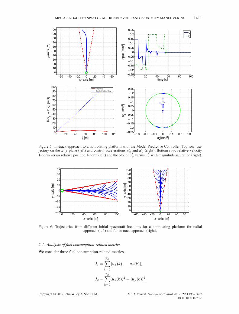
In the in-track approach, the spacecraft approaches the platform in the direction along the orbitaltrack. To simulate the in-track approach, the initial location of the spacecraft is chosen as.ıx0, ıy0/D .�10, 100/ (m) and the initial position of the docking port as .rx0, ry0/D .0, 2.5/ (m).The closed-loop responses are shown in Figure 5.

5.3. Trajectories from different initial locations

The initial location of the spacecraft is now varied within the LOS cone. The starting points consistof points on the boundaries of the LOS cone and points in the interior of LOS cone. The results areshown in Figure 6 for the radial approach and for the in-track approach. The trajectories near bothboundaries have similar curvature in both cases.

0 20 40 60 80 100−40

−30

−20

−10

0

10

20

30

40

x−axis [m]

y−ax

is [m

]

0 20 40 60 80 100−0.25

−0.2

−0.15

−0.1

−0.05

0

0.05

0.1

0.15

0.2

0.25

time [s]

inpu

t [m

/s2 ]

ux,

uy,

0 20 40 60 80 100 1200

10

20

30

40

50

60

70

80

90

100

ζ [m]

|δ v

x| +

|δ v

y| [m

/s]

TrajectoryConstraints boundary

−0.3 −0.2 −0.1 0 0.1 0.2 0.3−0.25

−0.2

−0.15

−0.1

−0.05

0

0.05

0.1

0.15

0.2

0.25

ux, [m/s2]

u y, [m/s

2 ]

Figure 4. Radial approach to a nonrotating platform with the Model Predictive Controller. Top row: tra-jectory on the x–y plane (left) and control accelerations u0x and u0y (right). Bottom row: relative velocity1-norm versus relative position 1-norm (left) and the plot of u0y versus u0x with magnitude saturation (right).



−60 −40 −20 0 20 40 600

10

20

30

40

50

60

70

80

90

100

x−axis [m]

y−ax

is [m

]

0 20 40 60 80 100−0.25

−0.2

−0.15

−0.1

−0.05

0

0.05

0.1

0.15

0.2

0.25

time [s]

inpu

t [m

/s2 ]

ux,

uy,

0 20 40 60 80 100 1200

10

20

30

40

50

60

70

80

90

100

ζ [m]

|δ v

x| + |δ

vy| [

m/s

]

TrajectoryConstraints boundary

−0.3 −0.2 −0.1 0 0.1 0.2 0.3−0.25

−0.2

−0.15

−0.1

−0.05

0

0.05

0.1

0.15

0.2

0.25

ux, [m/s2]

u y, [m

/s2 ]

Figure 5. In-track approach to a nonrotating platform with the Model Predictive Controller. Top row: tra-jectory on the x–y plane (left) and control accelerations u0x and u0y (right). Bottom row: relative velocity1-norm versus relative position 1-norm (left) and the plot of u0y versus u0x with magnitude saturation (right).

0 20 40 60 80 100−40

−30

−20

−10

0

10

20

30

40

x−axis [m]

y−ax

is [m

]

−60 −40 −20 0 20 40 600

102030405060708090

100

x−axis [m]

y−ax

is [m

]

Figure 6. Trajectories from different initial spacecraft locations for a nonrotating platform for radialapproach (left) and for in-track approach (right).

5.4. Analysis of fuel consumption-related metrics

We consider three fuel consumption-related metrics

J1 D

TdXkD0

jux.k/j C juy.k/j,

J2 D

TdXkD0

.ux.k//2C .uy.k//

2,



J3 D

TdXkD0

q.ux.k//2C .uy.k//2, (32)

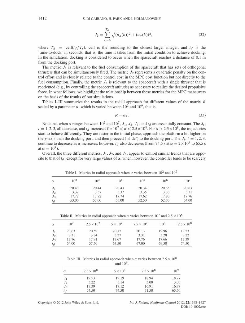
where Td D ceil.td=Ts/, ceil is the rounding to the closest larger integer, and td is the‘time-to-dock’ in seconds, that is, the time it takes from the initial condition to achieve docking.In the simulation, docking is considered to occur when the spacecraft reaches a distance of 0.1 mfrom the docking port.

The metric J1 is relevant to the fuel consumption of the spacecraft that has sets of orthogonalthrusters that can be simultaneously fired. The metric J2 represents a quadratic penalty on the con-trol effort and is closely related to the control cost in the MPC cost function but not directly to thefuel consumption. Finally, the metric J3 is relevant to the spacecraft with a single thruster that isreoriented (e.g., by controlling the spacecraft attitude) as necessary to realize the desired propulsiveforce. In what follows, we highlight the relationship between these metrics for the MPC maneuverson the basis of the results of our simulations.

Tables I–III summarize the results in the radial approach for different values of the matrix Rscaled by a parameter ˛, which is varied between 102 and 109, that is,

RD ˛I . (33)

Note that when ˛ ranges between 102 and 107, J1, J2, J3, and td are essentially constant. The Ji ,i D 1, 2, 3, all decrease, and td increases for 107 6 ˛ 6 2.5�108. For ˛ > 2.5�108, the trajectoriesstart to behave differently. They are faster in the initial phase, approach the platform a bit higher onthe y-axis than the docking port, and then proceed (‘slide’) to the docking port. The Ji , i D 1, 2, 3,continue to decrease as ˛ increases; however, td also decreases (from 74.5 s at ˛ D 2�108 to 65.5 sat ˛ D 109).

Overall, the three different metrics, J1,J2, and J3, appear to exhibit similar trends that are oppo-site to that of td , except for very large values of ˛, when, however, the controller tends to be scarcely

Table I. Metrics in radial approach when ˛ varies between 102 and 107.

˛ 102 103 104 105 106 107

J1 20.43 20.44 20.43 20.34 20.63 20.63J2 3.37 3.37 3.37 3.35 3.36 3.31J3 17.72 17.72 17.74 17.62 17.70 17.76td 53.00 53.00 53.00 52.50 52.50 54.00

Table II. Metrics in radial approach when ˛ varies between 107 and 2.5� 108.

˛ 107 2.5� 107 5� 107 7.5� 107 108 2.5� 108

J1 20.63 20.59 20.17 20.13 19.96 19.53J2 3.31 3.34 3.27 3.31 3.28 3.22J3 17.76 17.91 17.67 17.76 17.66 17.39td 54.00 57.50 63.50 67.00 69.50 74.50

Table III. Metrics in radial approach when ˛ varies between 2.5� 108

and 109.

˛ 2.5� 108 5� 108 7.5� 108 109

J1 19.53 19.19 18.94 18.77J2 3.22 3.14 3.08 3.03J3 17.39 17.12 16.91 16.77td 74.50 74.50 71.50 65.50



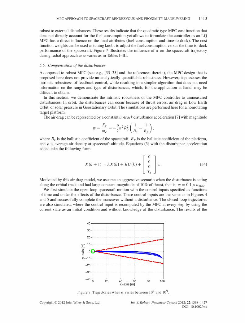
robust to external disturbances. These results indicate that the quadratic type MPC cost function thatdoes not directly account for the fuel consumption yet allows to formulate the controller as an LQMPC has a direct influence on the final attributes (fuel consumption and time-to-dock). The costfunction weights can be used as tuning knobs to adjust the fuel consumption versus the time-to-dockperformance of the spacecraft. Figure 7 illustrates the influence of ˛ on the spacecraft trajectoryduring radial approach as ˛ varies as in Tables I–III.

5.5. Compensation of the disturbances

As opposed to robust MPC (see e.g., [33–35] and the references therein), the MPC design that isproposed here does not provide an analytically quantifiable robustness. However, it possesses theintrinsic robustness of feedback control, while resulting in a simpler algorithm that does not needinformation on the ranges and type of disturbances, which, for the application at hand, may bedifficult to obtain.

In this section, we demonstrate the intrinsic robustness of the MPC controller to unmeasureddisturbances. In orbit, the disturbances can occur because of thrust errors, air drag in Low EarthOrbit, or solar pressure in Geostationary Orbit. The simulations are performed here for a nonrotatingtarget platform.

The air drag can be represented by a constant in-track disturbance acceleration [7] with magnitude

w DFy

mcD�

�

2n2R20

�1

Bc�

1

Bp

�,

where Bc is the ballistic coefficient of the spacecraft, Bp is the ballistic coefficient of the platform,and � is average air density at spacecraft altitude. Equations (3) with the disturbance accelerationadded take the following form:

NX.kC 1/D NA NX.k/C NB NU .k/C

264

0

0

0

Ts

375w. (34)

Motivated by this air drag model, we assume an aggressive scenario when the disturbance is actingalong the orbital track and had large constant magnitude of 10% of thrust, that is, w D 0.1� umax.

We first simulate the open-loop spacecraft motion with the control inputs specified as functionsof time and under the effects of the disturbance. These control inputs are the same as in Figures 4and 5 and successfully complete the maneuver without a disturbance. The closed-loop trajectoriesare also simulated, where the control input is recomputed by the MPC at every step by using thecurrent state as an initial condition and without knowledge of the disturbance. The results of the

0 20 40 60 80 100−40

−30

−20

−10

0

10

20

30

40

x−axis [m]

y−ax

is [m

]

Figure 7. Trajectories when ˛ varies between 102 and 109.



open-loop and closed-loop maneuvers for radial and in-track approach by the spacecraft affectedby the disturbance are shown in Figures 8 and 9. With the open-loop control, the spacecraft fails tocomplete the maneuver because of the disturbances. On the other hand, the MPC controller is ableto successfully guide the spacecraft despite these disturbances: The final error is about 1.2 cm forboth radial and in-track maneuvers.

Figures 10 and 11 illustrate additional responses to disturbances for the radial and in-trackapproaches, respectively. We consider the cases of (i) constant disturbance vector with componentsof magnitude (0.1 � umax) on both x and y axis and (ii) random disturbance in acceleration actua-tion amplitude and direction. In the second case, the disturbance simulates errors in thrust direction,for instance because of some error in the attitude control, and amplitude, for instance because ofrealization of the continuous thrust through thrust pulses [7]. In this case, the actuated spacecraftacceleration is

ur.k/D satumax2 .R�.k/U

�.0jk//,

u.k/D satumax2 ..1C ud .k//ur.k//,

where satumax2 denotes the saturation in 2-norm by directionality preserving scaling (11), R� D�

cos.�/ � sin.�/sin.�/ cos.�/

�is the matrix producing a rotation of angle � , and �.k/ 2 Œ��

6, �6�, ud .k/ 2

Œ�0.15, 0.15� are independent, uniformly distributed discrete-time random variables whose valueschange every 5 s. In radial and in-track approaches, the MPC controller is able to successfully com-pensate the effect of these disturbances. The trajectories obtained for 10 simulations with randomdisturbances on both radial and in-track approaches are shown in Figure 12. Finally, in our simula-tions, actuation disturbances of up to˙25% magnitude and˙45 deg direction appear to be tolerablefor the proposed control strategy.

0 20 40 60 80 100

−10

0

10

20

30

40

50

60

70

80

x−axis [m]

y−ax

is [m

]

0 20 40 60 80 100−0.25

−0.2

−0.15

−0.1

−0.05

0

0.05

0.1

0.15

0.2

0.25

time [s]

inpu

t [m

/s2 ]

UxUy

0 20 40 60 80 100−40

−30

−20

−10

0

10

20

30

40

x−axis [m]

y−ax

is [m

]

0 20 40 60 80 100−0.25

−0.2

−0.15

−0.1

−0.05

0

0.05

0.1

0.15

0.2

0.25

time [s]

inpu

t [m

/s2 ]

UxUy

Figure 8. Radial approach subject to disturbances. Top row: open-loop trajectory (left) and open-loopcontrol accelerations (right). Bottom row: closed-loop trajectory (left) and closed-loop control accelera-

tions (right).



−60 −40 −20 0 20 40 600

10

20

30

40

50

60

70

80

90

100

x−axis [m]

y−ax

is [m

]

0 20 40 60 80 100−0.25

−0.2

−0.15

−0.1

−0.05

0

0.05

0.1

0.15

0.2

0.25

time [s]

inpu

t [m

/s2 ]

UxUy

−60 −40 −20 0 20 40 600

10

20

30

40

50

60

70

80

90

100

x−axis [m]

y−ax

is [m

]

0 20 40 60 80 100−0.25

−0.2

−0.15

−0.1

−0.05

0

0.05

0.1

0.15

0.2

0.25

time [s]

inpu

t [m

/s2 ]

UxUy

Figure 9. In-track approach subject to disturbances. Top row: open-loop trajectory (left) and open-loopcontrol accelerations (right). Bottom row: closed-loop trajectory (left) and closed-loop control accelera-

tions (right).

5.6. Explicit Model Predictive Control

When MPC is applied to linear systems with linear constraints and quadratic cost function, the con-trol law can be explicitly computed by multiparametric quadratic programming (see [20, 21]). TheMPC control law, NUMPC. NX/, is a piecewise affine state feedback, specified through the state-spacepartitioning into polyhedral regions and an affine state feedback law assigned to each region. Withthe use of the explicit MPC control law, the need to perform online optimization and to validate andembed the QP solver in the control software is avoided.

For the case where the target platform does not rotate and the angle of the LOS cone is knownand fixed, we can design an explicit MPC controller. Because the coefficients of NC in Equation (20)change discretely depending on the current state, a slightly modified synthesis procedure is required,similarly to [36].

First, we enumerate the possible values of NC in (19), caused by the changing signs of the currentstate in (15) (or (16)), hence, obtaining the set of matrices, C D

®NCh¯qhD1

. Then, we compute thecontrol laws �MPC.i , NX/, i D 1, : : : , q, by applying multiparametric programming to the MPC prob-lem, where NC D NCi is a constant. Because each of the corresponding MPC optimization problemsis a standard quadratic program, each feedback law has a piecewise affine form

�MPC.i , NX/D FijNX CGij

j WH ijNX 6Kij ,

(35)

where j 2 Ji , Ji D ¹1, : : : , qiº and qi is the number of regions of the MPC law associated to thecase NC D NCi . Note also that the switching conditions on the NC coefficients are independent of thecurrent control input and can be encoded by linear inequalities, such that NC D NCi if and only if



0 20 40 60 80 100−40

−30

−20

−10

0

10

20

30

40

x−axis [m]

y−ax

is [m

]

0 20 40 60 80 100−0.25

−0.2

−0.15

−0.1

−0.05

0

0.05

0.1

0.15

0.2

0.25

time [s]

inpu

t [m

/s2 ]

UxUy

0 20 40 60 80 100−40

−30

−20

−10

0

10

20

30

40

x−axis [m]

y−ax

is [m

]

0 20 40 60 80 100−0.25

−0.2

−0.15

−0.1

−0.05

0

0.05

0.1

0.15

0.2

0.25

time [s]

inpu

t [m

/s2 ]

UxUyUactxUacty

Figure 10. Radial approach subject to disturbances. Top row: constant disturbance in x–y direction. Closed-loop trajectory (left) and closed-loop control accelerations (right). Bottom row: random magnitude dis-turbance in x–y direction. Closed-loop trajectory (left) and closed-loop control accelerations (solid) and

actuated accelerations (dash) (right).

Hi NX 6Ki . Thus, the q control laws can be merged into a single piecewise affine function

uD F ijNX.k/CGij , (36a)

i , j WHi NX.k/6Ki , (36b)

H ijNX.k/6Kij , (36c)

where (36c) selects the control law that is active, (36b) selects the control law region that is currentlyactive, and (36a) is evaluated to obtain the control input.

To construct the explicit solution, we choose the implementation of MPC controller based on (14)that gives q D 16, and hence, 16 control laws are merged in (36). The 16 piecewise affine feedbackcontrol laws are obtained by the 16 choices for the signs‘ of NC43, NC44, NC45, and NC46.

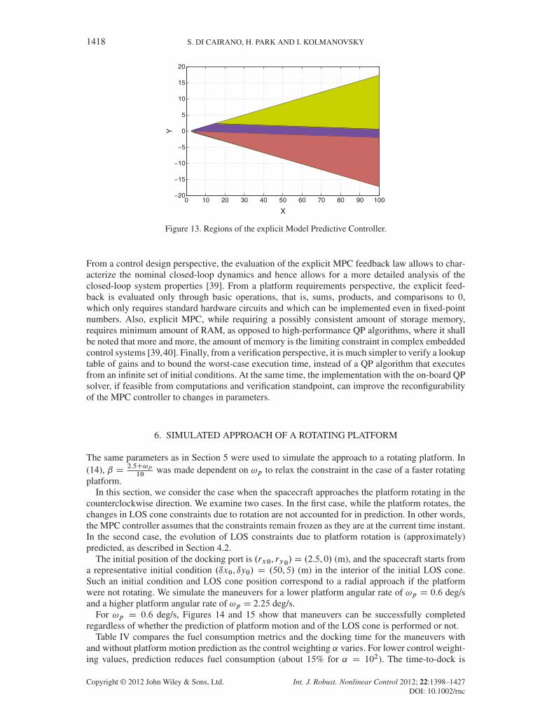
For our MPC controller, the total number of polyhedral regions in (36) for the case where allfour components of the matrix NC switch (this is 16 control laws case) is 3068. Figure 13 shows thecross-section of the regions in x � y plane, computed for zero velocity and docking port located at.2.5, 0/. The number of regions appears to be acceptable and suggests that explicit MPC solutionscan be feasible for automation of spacecraft rendezvous and proximity maneuvers. Furthermore, thecomplexity of the polyhedral partitioning can be reduced by eliminating small regions and expand-ing the neighboring ones. In fact, it was verified that about a third of the regions have Chebyshevradius smaller than 10�3 and can be eliminated. The elimination of these regions induces mini-mal perturbations to the closed-loop system, and these perturbations are restricted only to area ofthe removed regions. Also, in general, the controller uses most frequently (i.e., more than 99% oftimes) a much smaller subset of regions, usually 10%–20% of the total, which can be identified

‘Here, we apply a slightly modified definition of sgn.�/, where sgn.0/D 1.



−60 −40 −20 0 20 40 600

10

20

30

40

50

60

70

80

90

100

x−axis [m]

y−ax

is [m

]

0 20 40 60 80 100−0.25

−0.2

−0.15

−0.1

−0.05

0

0.05

0.1

0.15

0.2

0.25

time [s]

inpu

t [m

/s2 ]

UxUy

−60 −40 −20 0 20 40 600

10

20

30

40

50

60

70

80

90

100

x−axis [m]

y−ax

is [m

]

0 20 40 60 80 100−0.25

−0.2

−0.15

−0.1

−0.05

0

0.05

0.1

0.15

0.2

0.25

time [s]

inpu

t [m

/s2 ]

UxUyUactxUacty

Figure 11. In-track approach subject to disturbances. Top row: constant disturbance in x–y direction.Closed-loop trajectory (left) and closed-loop control accelerations (right). Bottom row: random magnitudedisturbance in x–y direction. Closed-loop trajectory (left) and closed-loop control accelerations (solid) and

actuated accelerations (dash) (right).

0 20 40 60 80 100−40

−30

−20

−10

0

10

20

30

40

x−axis [m]

y−ax

is [m

]

−60 −40 −20 0 20 40 600

10

20

30

40

50

60

70

80

90

100

x−axis [m]

y−ax

is [m

]

Figure 12. Repeated simulations with random disturbances on thrust actuation. Closed-loop radial approachtrajectories (left) and closed-loop in-track approach trajectories (right).

by extensive simulations. With these approaches, the controller data memory requirements can bereduced to fit the platform computational resources.

If instead we use simplified constraints (16), we can reduce the effort for computation and stor-age to q D 4 piecewise affine feedback control laws. A minor drawback with this approach is thatthe parameter vector in the multiparametric programming algorithm (see [20]) needs to include thevariable �.k/ defined in (17) and hence the feedback law has one extra dimension.

Remark 3It is important to briefly recall the benefits that can be obtained by deploying the explicit MPCfeedback law in complex embedded control systems [37, 38], rather than the QP-based algorithm.



0 10 20 30 40 50 60 70 80 90 100−20

−15

−10

−5

0

5

10

15

20

X

Y

Figure 13. Regions of the explicit Model Predictive Controller.

From a control design perspective, the evaluation of the explicit MPC feedback law allows to char-acterize the nominal closed-loop dynamics and hence allows for a more detailed analysis of theclosed-loop system properties [39]. From a platform requirements perspective, the explicit feed-back is evaluated only through basic operations, that is, sums, products, and comparisons to 0,which only requires standard hardware circuits and which can be implemented even in fixed-pointnumbers. Also, explicit MPC, while requiring a possibly consistent amount of storage memory,requires minimum amount of RAM, as opposed to high-performance QP algorithms, where it shallbe noted that more and more, the amount of memory is the limiting constraint in complex embeddedcontrol systems [39,40]. Finally, from a verification perspective, it is much simpler to verify a lookuptable of gains and to bound the worst-case execution time, instead of a QP algorithm that executesfrom an infinite set of initial conditions. At the same time, the implementation with the on-board QPsolver, if feasible from computations and verification standpoint, can improve the reconfigurabilityof the MPC controller to changes in parameters.

6. SIMULATED APPROACH OF A ROTATING PLATFORM

The same parameters as in Section 5 were used to simulate the approach to a rotating platform. In(14), ˇ D 2.5C!p

10was made dependent on !p to relax the constraint in the case of a faster rotating

platform.In this section, we consider the case when the spacecraft approaches the platform rotating in the

counterclockwise direction. We examine two cases. In the first case, while the platform rotates, thechanges in LOS cone constraints due to rotation are not accounted for in prediction. In other words,the MPC controller assumes that the constraints remain frozen as they are at the current time instant.In the second case, the evolution of LOS constraints due to platform rotation is (approximately)predicted, as described in Section 4.2.

The initial position of the docking port is .rx0, ry0/D .2.5, 0/ (m), and the spacecraft starts froma representative initial condition .ıx0, ıy0/ D .50, 5/ (m) in the interior of the initial LOS cone.Such an initial condition and LOS cone position correspond to a radial approach if the platformwere not rotating. We simulate the maneuvers for a lower platform angular rate of !p D 0.6 deg/sand a higher platform angular rate of !p D 2.25 deg/s.

For !p D 0.6 deg/s, Figures 14 and 15 show that maneuvers can be successfully completedregardless of whether the prediction of platform motion and of the LOS cone is performed or not.

Table IV compares the fuel consumption metrics and the docking time for the maneuvers withand without platform motion prediction as the control weighting ˛ varies. For lower control weight-ing values, prediction reduces fuel consumption (about 15% for ˛ D 102). The time-to-dock is



0 10 20 30 40 50−25

−20

−15

−10

−5

0

5

10

15

20

25

x−axis [m]

y−ax

is [m

]

−6 −4 −2 0 2 4 6−5

−4

−3

−2

−1

0

1

2

3

4

5

x−axis [m]

y−ax

is [m

]

0 20 40 60 80 100−0.25

−0.2

−0.15

−0.1

−0.05

0

0.05

0.1

0.15

0.2

0.25

time [s]

inpu

t [m

/s2 ]

ux,

uy,

−0.3 −0.2 −0.1 0 0.1 0.2 0.3−0.25

−0.2

−0.15

−0.1

−0.05

0

0.05

0.1

0.15

0.2

0.25

ux, [m/s2]

uy, [m

/s2 ]

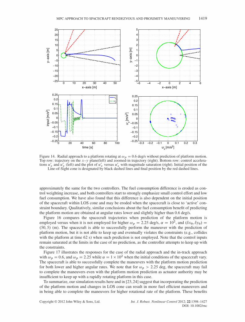
Figure 14. Radial approach to a platform rotating at !p D 0.6 deg/s without prediction of platform motion.Top row: trajectory on the x–y plane(left) and zoomed-in trajectory (right). Bottom row: control accelera-tions u0x and u0y (left) and the plot of u0y versus u0x with magnitude saturation (right). Initial position of the

Line-of-Sight cone is designated by black dashed lines and final position by the red dashed lines.

approximately the same for the two controllers. The fuel consumption difference is eroded as con-trol weighting increase, and both controllers start to strongly emphasize small control effort and lowfuel consumption. We have also found that this difference is also dependent on the initial positionof the spacecraft within LOS cone and may be eroded when the spacecraft is close to ‘active’ con-straint boundary. Qualitatively, similar conclusions about the fuel consumption benefit of predictingthe platform motion are obtained at angular rates lower and slightly higher than 0.6 deg/s.

Figure 16 compares the spacecraft trajectories when prediction of the platform motion isemployed versus when it is not employed for higher !p D 2.25 deg/s, ˛ D 102, and .ıx0, ıy0/ D.50, 5/ (m). The spacecraft is able to successfully perform the maneuver with the prediction ofplatform motion, but it is not able to keep up and eventually violates the constraints (e.g., collideswith the platform at time 62 s) when such prediction is not employed. Note that the control inputsremain saturated at the limits in the case of no prediction, as the controller attempts to keep up withthe constraints.

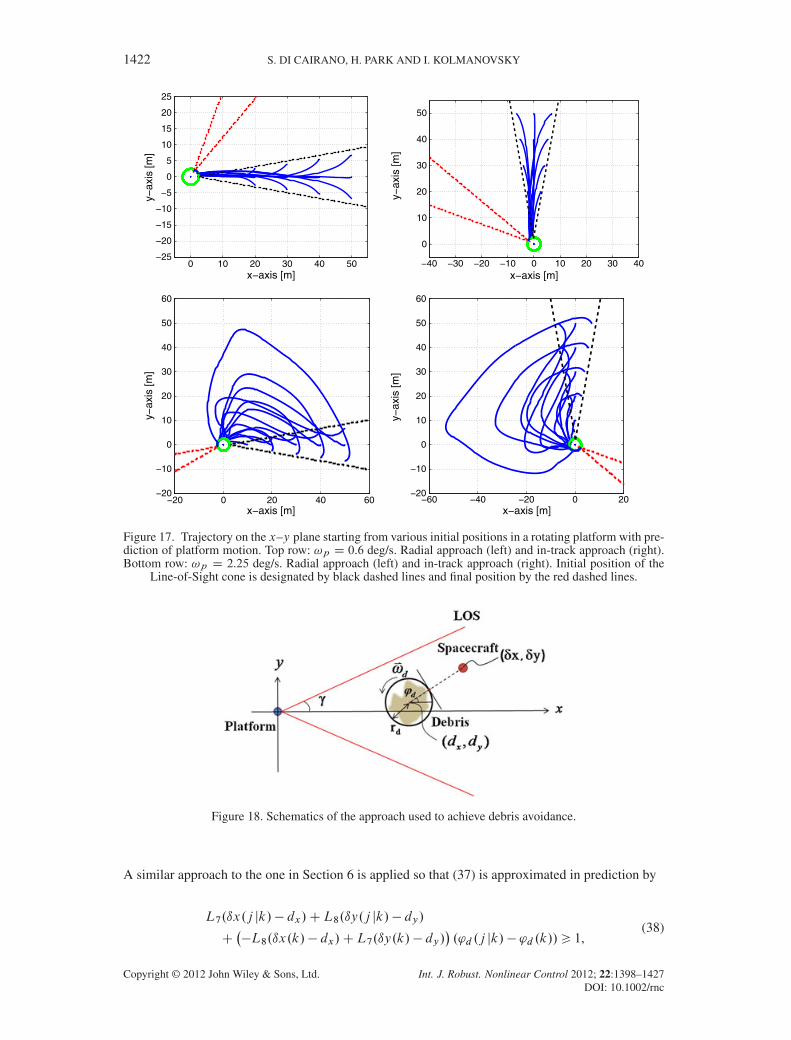
Figure 17 illustrates the responses for the case of the radial approach and the in-track approachwith !p D 0.6, and !p D 2.25 while ˛ D 1� 102 when the initial conditions of the spacecraft vary.The spacecraft is able to successfully complete the maneuvers with the platform motion predictionfor both lower and higher angular rates. We note that for !p > 2.25 deg, the spacecraft may failto complete the maneuvers even with the platform motion prediction as actuator authority may beinsufficient to keep up with a rapidly rotating platform in this case.

To summarize, our simulation results here and in [23,24] suggest that incorporating the predictionof the platform motion and changes in LOS cone can result in more fuel efficient maneuvers andin being able to complete the maneuvers for higher rotational rate of the platform. These benefits



0 10 20 30 40 50−25

−20

−15

−10

−5

0

5

10

15

20

25

x−axis [m]

y−ax

is [m

]

−6 −4 −2 0 2 4 6−5

−4

−3

−2

−1

0

1

2

3

4

5

x−axis [m]

y−ax

is [m

]

0 20 40 60 80 100−0.25

−0.2

−0.15

−0.1

−0.05

0

0.05

0.1

0.15

0.2

0.25

time [s]

ux,

uy,

−0.3 −0.2 −0.1 0 0.1 0.2 0.3−0.25

−0.2

−0.15

−0.1

−0.05

0

0.05

0.1

0.15

0.2

0.25

ux, [m/s2]

u y, [m/s

2 ]

inpu

t [m

/s2 ]

Figure 15. Radial approach platform rotating at !p D 0.6 deg/s with prediction of platform motion. Toprow: trajectory on the x–y plane(left) and zoomed-in trajectory (right). Bottom row: control accelerationsu0x and u0y (left) and the plot of u0y versus u0x with magnitude saturation (right). Initial position of the


Table IV. Fuel consumption-related metrics and docking time versus ˛.

!p D 0.6 deg/s ˛ 102 103 104 105 106 107 5� 107 108 5� 108

J1 17.44 18.16 15.61 17.74 15.66 14.28 13.49 13.16 12.55Nonpredicted J2 2.36 2.50 2.14 2.41 2.15 1.88 1.79 1.76 1.63constraints J3 13.33 13.94 12.18 13.59 12.29 11.51 11.20 11.10 10.64

td (s) 40.50 40.50 40.50 40.50 40.50 42.00 51.00 57.50 63.50

J1 14.35 14.34 14.28 14.38 14.04 13.65 13.12 12.94 12.13Predicted J2 1.93 1.93 1.92 1.93 1.87 1.76 1.72 1.70 1.54constraints J3 11.57 11.57 11.54 11.58 11.41 11.17 11.00 10.91 10.27

td (s) 40.50 40.50 40.50 40.50 41.00 42.00 51.50 57.50 63.50

are more pronounced for medium range of !p , and are eroded for very low values of !p and as !pincreases to larger values, which exceed the actuators capabilities.

7. COLLISION AVOIDANCE MANEUVERS

In this section, we consider the additional objective of avoiding debris on the spacecraft rendezvouspath. There are more than 22,000 debris of 10 cm and longer orbiting the Earth today, and thisnumber is growing. Collision with orbital debris is a serious threat that can damage the spacecraft.Several collision risk assessment methods have been developed, see for example, [41–45] and ref-erences therein, along with debris collision avoidance strategies, see for example, [41, 46, 47] and



−20 0 20 40 60−40

−30

−20

−10

0

10

20

30

40

x−axis [m]

y−ax

is [m

]

0 10 20 30 40 50 60−0.25

−0.2

−0.15

−0.1

−0.05

0

0.05

0.1

0.15

0.2

0.25

time [s]

inpu

t [m

/s2 ]

ux,

uy,

−20 0 20 40 60−40

−30

−20

−10

0

10

20

30

40

x−axis [m]

y−ax

is [m

]

0 20 40 60 80 100−0.25

−0.2

−0.15

−0.1

−0.05

0

0.05

0.1

0.15

0.2

0.25

time [s]

inpu

t [m

/s2 ]

ux,

uy,

Figure 16. Radial approach to a platform rotating at with !p D 2.25 deg/s. Top row: plots without pre-diction of platform motion. Trajectory on the x–y plane (left) and control accelerations u0x and u0y (right).Bottom row: plots with prediction of platform motion. Trajectory (left) and control accelerations (right).Initial position of the Line-of-Sight cone is designated by black dashed lines and final position by the red

dashed lines.

references therein. In [46, 48], for instance, collision avoidance strategies for polyhedral objects asobstacles have been developed on the basis of mixed-integer linear programming.

To incorporate debris avoidance in our MPC approach, we assume that the debris can be coveredby a virtual disk of radius rd centered at .dx , dy/ (m). See Figure 18.

7.1. Model Predictive Controller design for debris avoidance

Our approach to debris avoidance is based on covering the debris by a disk and assuming that this‘virtual’ disk slowly rotates with angular rate !d (rad/s). Referring to Figure 18, we impose theconstraint forcing the spacecraft to remain in a specified half-plane relative to a tangent line to thedisk. As the tangent line rotates with the disk, the constraint is dynamically reconfigured and variesin time. For simplicity, we assume here that the docking port does not rotate, and it is at the originof the reference frame, that is, .rx , ry/D .0, 0/, .�x , �y/D .ıx, ıy/.

At the activation of the constraint, the disk tangent line is perpendicular to the line betweenthe spacecraft location, .ıx.0/, ıy.0// (m), and the center of the disk, .dx , dy/. The angle 'd .0/is defined as the angle between the x-axis and the normal to the tangent line so that 'd .0/ D

tan�1�ıy.0/�dyıx.0/�dx

. Then, 'd .k C 1/ D 'd .k/ C !dkTs , and the debris avoidance constraint is

given by

cos'd .k/

rd.ıx.k/� dx/C

sin'd .k/

rd.ıy.k/� dy/> 1. (37)



0 10 20 30 40 50−25

−20

−15

−10

−5

0

5

10

15

20

25

x−axis [m]

y−ax

is [m

]

−40 −30 −20 −10 0 10 20 30 40

0

10

20

30

40

50

x−axis [m]

y−ax

is [m

]

−20 0 20 40 60−20

−10

0

10

20

30

40

50

60

x−axis [m]

y−ax

is [m

]

−60 −40 −20 0 20−20

−10

0

10

20

30

40

50

60

x−axis [m]

y−ax

is [m

]

Figure 17. Trajectory on the x–y plane starting from various initial positions in a rotating platform with pre-diction of platform motion. Top row: !p D 0.6 deg/s. Radial approach (left) and in-track approach (right).Bottom row: !p D 2.25 deg/s. Radial approach (left) and in-track approach (right). Initial position of the


Figure 18. Schematics of the approach used to achieve debris avoidance.

A similar approach to the one in Section 6 is applied so that (37) is approximated in prediction by

L7.ıx.j jk/� dx/CL8.ıy.j jk/� dy/

C��L8.ıx.k/� dx/CL7.ıy.k/� dy/

�.'d .j jk/� 'd .k//> 1,

(38)



where

L7 Dcos'd .k/

rd, L8 D

sin'd .k/

rd,

'd .j jk/' 'd .k/C P'd .k/jTs ,

and j 2 Z0C denotes a future instant with respect to k. Debris constraint (38) is deactivated once'd becomes equal to 'd .0/C so that the constraint does not interfere with the spacecraft motionafter it passes the debris.

Similarly to (28) and (29), the state vector for debris avoidance maneuver has the form

OX D�ıx ıy ı Px ı Py dx dy rdx rdy ´1 ´2

�T,

and the model is represented by

OX.j C 1jk/D OA OX.j jk/C OB OU.j jk/, (39a)

OY .j jk/D OC OX.j jk/C OD OU .j jk/, (39b)

where

OAD

0B@

Ad 04�2 04�2 04�202�4 I 02�2 02�202�4 02�2 d 02�202�4 02�2 02�2 ‚

1CA , OB D NB , OD D ND,

OU D NU , � is defined in (27),

OC D

0BB@

L7 L8 0 0 �L7 �L8 0 0 0 OC1sin � � cos � 0 0 0 0 0 0 0 0

sin � cos � 0 0 0 0 0 0 0 0OC2 OC3 OC4 OC5 0 0 0 0 0 0

1CCA ,

and

d D

�cos.!dTs/ � sin.!dTs/sin.!dTs/ cos.!dTs/

�,

OC1 D L8.ıx.k/� dx/CL7.ıy.k/� dy/,

OC2 D sgn.ıx.k//, OC3 D sgn.ıy.k//,

OC4 D��sgn.ı Px.k//, OC5 D��sgn.ı Py.k//,

and where the constraint

OY .j jk/> OYmin, OYmin D�1 0 0 �ˇ

�T, (40)

is imposed on the system output, representing the LOS constraints, the soft-docking constraint withrespect to the platform, and the debris avoidance constraint.



Thus, for the debris avoidance case, the MPC optimal control problem is formulated as

minOU.k/

OX.NJ jk/T OP OX.NJ jk/C

NJ�1XjD0

OX.j jk/T OQ OX.j jk/C OU .j jk/T OR OU .j jk/,

(41a)

s.t. OX.j C 1jk/D OA OX.j jk/C OB OU .j jk/, (41b)

OY .j jk/D OC OX.j jk/C OD OU .j jk/, (41c)

OX.0jk/D OX.k/, (41d)

OU .j jk/D OK OX.j jk/, j DNU C 1, : : : ,NJ � 1, (41e)

OY .j jk/> OYmin.k/, j D 0, : : : ,NC , (41f)

OU .j jk/> OUmin, j D 0, : : : ,NU , (41g)

OU .j jk/6 OUmax, j D 0, : : : ,NU , (41h)

where OU.k/D°OU .0jk/, � � � , OU .NU jk/

±,

OP D

�P 04�6

06�4 06�6

�, OQD

�Q 04�6

06�4 06�6

�, ORD NR, OK D

�K 02�6

�,

and the input constraints in (41) are defined by (10).

0 10 20 30 40 50 60−25

−20

−15

−10

−5

0

5

10

15

20

25

x−axis [m]

y−ax

is [m

]

0 10 20 30 40 50−0.25

−0.2

−0.15

−0.1

−0.05

0

0.05

0.1

0.15

0.2

0.25

time [s]

inpu

t [m

/s2 ]

ux,

uy,

0 10 20 30 40 50 60−25

−20

−15

−10

−5

0

5

10

15

20

25

x−axis [m]

y−ax

is [m

]

0 10 20 30 40 50−0.25

−0.2

−0.15

−0.1

−0.05

0

0.05

0.1

0.15

0.2

0.25

time [s]

inpu

t [m

/s2 ]

ux,

uy,

Figure 19. Comparison of the maneuvers. Top row: trajectory on the x–y plane without debris (left) andcontrol accelerations u0x and u0y without debris (right). Bottom row: trajectory on the x–y plane with debris

(left) and control accelerations u0x and u0y (right) with debris.



0 10 20 30 40 50 60−25

−20

−15

−10

−5

0

5

10

15

20

25

x−axis [m]

y−ax

is [m

]

0 10 20 30 40 50 60−25

−20

−15

−10

−5

0

5

10

15

20

25

x−axis [m]

y−ax

is [m

]

Figure 20. Trajectories from various initial positions without debris (left) and with debris (right).

Table V. Costs and docking time in maneuvers with and without debrisavoidance.

J1 J2 J3 td

Without debris 17.88 3.03 14.77 45.50With debris 21.03 3.53 16.18 53.00

7.2. Simulation results

Simulation results are now presented for rd D 2 m. Other parameters are the same as the ones inSection 6. The debris is located at .dx , dy/ D .40, 0/ (m), and the initial location of the spacecraftis .ıx0, ıy0/ D .60, 5 (m). The docking port is located at the origin of the reference frame and isrepresented here as a point mass. The angular rate of the ‘virtual’ disk, !d , was varied between5 deg and 15 deg, and the best value of !d D 12 deg/s was determined in simulations on the basisof a trade-off between maneuver feasibility (in terms of satisfying the imposed constraints) andspeed. Figure 19 compares the trajectories of the spacecraft when there is no debris and when thespacecraft performs a rendezvous while avoiding debris. Note that the debris is placed at a locationthat makes infeasible the trajectory of the no-debris case. The ‘x’ symbol represents the initial pointof activation of the tangent line constraint. The constraint is deactivated after the disk covering thedebris has rotated rad. The line tangent to the virtual disk in Figure 19 is in the position after thedisk rotated rad, and the debris avoidance constraint is deactivated. Figure 20 illustrates debrisavoidance maneuvers for various initial positions of the spacecraft.

We also report the three fuel consumption-related metrics in (32) and the time-to-dock for the casewith and without the debris in Table V. The debris avoidance results in increased fuel consumptionand longer maneuver time.

8. CONCLUSIONS

In this paper, we have considered rendezvous and proximity maneuvering between a spacecraft and(a potentially rotating/tumbling) target platform. MPC was utilized to enforce velocity of approach(soft-docking), LOS cone, and thrust magnitude constraints. The problem was treated in an LQ MPCframework without introducing integer variables so that the finite horizon optimization problem canbe solved by QP algorithms, which are known to be efficient and computationally affordable. Toachieve this, we have employed dynamically reconfigurable linear constraints. We have demon-strated through simulations that the MPC controller is capable of planning efficient maneuvers,while enforcing all the imposed constraints, and of compensating for the effects of significant dis-turbances such as those that may be caused by thrust errors, air drag, or solar pressure. In addition,we have analyzed the dependence of fuel consumption and ‘time-to-dock’ on the weights of theMPC cost function by using three different metrics. The weights of the MPC cost function, for



example, the scaling factor on the control weighting matrix, have been shown to have a direct influ-ence over the trade-off between the fuel consumption and the docking time. For the case when theplatform is not rotating and the LOS cone angle is fixed and known, an explicit MPC solution canbe generated offline for on-board use, hence, avoiding the need for the deployment and validationof the QP solver in the spacecraft software. For the case when the target platform is rotating, ourresults suggest that predicting the motion of the docking port and of the associated changes in theLOS constraint permits to perform maneuvers initiated when the spacecraft is further away from theplatform and when the platform is rotating/tumbling at a higher rate. We have also shown that byincorporating such a prediction into the MPC problem formulation, the fuel consumption is reduced.Finally, we have demonstrated that related ideas can be applied for debris avoidance during therendezvous maneuver. The extensions to more general in and out-of-plane spacecraft motion and tothree dimensional spacecraft and platform rotations will be pursued in future works.

REFERENCES

1. Goodman J. History of space shuttle rendezvous and proximity operations. Jounal of Spacecraft and Rockets 2006;43(5):944–959.

2. Polites M. Technology of automated rendezvous and capture in space. Jounal of Spacecraft and Rockets 1999;36(2):280–291.

3. Woffinden D, Geller D. Navigating the road to autonomous orbital rendezvous. Jounal of Spacecraft and Rockets2007; 44(4):898–909.

4. Aldrin E, Jr. Line-of-sight guidance techniques for manned orbital rendezvous. Sc.D. Thesis, Massachusetts Instituteof Technology, USA, 1963.

5. Breger L, How J. Safe trajectories for autonomous rendezvous of spacecraft. Journal of Guidance, Control, andDynamics 2008; 5:31.

6. Clark F, Spehar P, Brazzel J, Hinkel H. Laser-based relative navigation and guidance for space shuttle proximityoperation. Advances in the Astronautical Sciences 2003; 113:732–737.

7. Fehse W. Automated Rendezvous and Docking of Spacecraft. Cambridge Aerospace Series: Cambridge, UK, 2003.8. Bryson A. Linear feedback solutions for minimum effort interception, rendezvous, and soft landing. AIAA Jounal

1965; 3(8):1542–1544.9. Coverstone-Carroll V. Detumbling and reorienting underactuated rigid spacecraft. Journal of Guidance, Control, and

Dynamics 1996; 3:19.10. Clohessy W, Wiltshire R. Terminal guidance system for satellite rendezvous. Journal of Aerospace Sciences 1960;

27(9):653–658.11. Luo Y, Tang G. Spacecraft optimal rendezvous controller design using simulated annealing. Aerospace Science and

Technology 2005; 9:732–737.12. Miele A, Weeks M, Circia M. Optimal trajectories for spacecraft rendezvous. Journal of Optimization Theory and

Applications 2007; 132(3):353–376.13. Kong E, Nolet S, Miller D. Autonomous docking algorithm development and experimentation using the SPHERES

testbed. Proceedings of SPIE Defense and Security Symposium, Orlando, Florida, 2004.14. Richards A, How J. Performance evaluation of rendezvous using model predictive control. AIAA Guidance,

Navigation, and Control Conference and Exhibit, AIAA Paper 2003-5507, Austin, Texas, 2003; 1–9.15. Hartley E. Model predictive control for spacecraft rendezvous. Ph.D. Dissertation, University of Cambridge, UK,

2010.16. Di Cairano S, Bemporad A. Model predictive control tuning by controller matching. IEEE Transactions on Automatic

Control 2010; 55(1):185–190.17. Singh L, Bortolami S, Page L. Optimal guidance and thruster control in orbital approach and rendezvous for dock-

ing using model predictive control. AIAA Guidance, Navigation, and Control Conference and Exhibit, AIAA Paper2010-7754, Toronto, Canada, 2010; 1–15.

18. Holzinger M, DiMatteo J, Schwartz J, Milam M. Passively safe receding horizon control for satellite proximityoperations. 47th IEEE Conference on Decision and Control, Cancun, Mexico, 2008; 3433–3440.

19. Nocedal J, Wright S. Numerical Optimization. Springer: New York, 2006.20. Bemporad A, Morari M, Dua V, Pistikopoulos E. The explicit linear quadratic regulator for constrained systems.

Automatica 2002; 38(1):3–20.21. Borrelli F, Bemporad A, Morari M. Model predictive control base on linear programming - the explicit solutions.

IEEE Transactions on Automatic Control 2002; 47(12):1974–1985.22. Park H, Di Cairano S, Kolmanovsky I. Model Predictive Control of spacecraft docking with a non-rotating platform.

IFAC 18th World Congress, Milano, Italy, 2011; 8485–8490.23. Park H, Di Cairano S, Kolmanovsky I. Model Predictive Control for spacecraft rendezvous and docking with a rotat-

ing/tumbling platform and for debris avoidance. American Control Conference, San Francisco, California, 2011;1922–1927.



24. Park H, Di Cairano S, Kolmanovsky I. Linear quadratic Model Predicitve Control approach to spacecraft rendezvousand docking. 21st AAS/AAIA Space Flight Mechnics Meeting, New Orleans, Louisiana, 2011.

25. Clarke D, Mohtadi C, Tuffs P. Generalized predictive control—part I the basic algorithm. Automatica 1987;23(2):137–148.

26. Clarke D, Mohtadi C, Tuffs P. Generalized predictive control—part II extensions and interpretations. Automatica1987; 23(2):149–160.

27. Wie B. Spacecraft dynamics and control, 2010. 2nd Edition AIAA.28. IBM ILOG CPLEX V12.1: User’s manual for CPLEX, 2009. International Business Machines Corporation.29. Boyd S, Vandenberghe L. Convex Optimization. Cambridge University Press: Cambridge, UK, 2004.30. Di Cairano S, Bemporad A, Kolmanovsky I, Hrovat D. Model predictive control of magnetically actuated mass spring

damper for automotive applications. International Journal of Control 2007; 80(11):1701–1716.31. Maciejowski J. Predictive Control with Constraints. Prentice Hall: London, 2000.32. Mayne DQ, Rawlings JB, Rao CV, Scokaert POM. Constrained model predictive control: stability and optimality.

Automatica 2000; 36(6):789–814.33. Mayne DQ, Seron MM, Rakovic SV. Robust model predictive control of constrained linear systems with bounded

disturbances. Automatica 2005; 41(2):219–224.34. Kothare MV, Balakrishnan V, Morari M. Robust constrained model predictive control using linear matrix

inequalities. Automatica 1996; 32(10):1361–1379.35. Bemporad A, Morari M. Robust model predictive control: a survey. In Robustness in Identification and Control,

Vol. 245, Garulli A, Tesi A (eds), Lect. Notes in Control and Inf. Sciences: Springer, London, 1999; 207–226.36. Di Cairano S, Tseng H, Bernardini D, Bemporad A. Steering vehicle control by switched model predictive control.

6th IFAC Symposium on Advances in Automotive Control, Munich, Germany, 2010; 1–6.37. Di Cairano S, Yanakiev D, Bemporad A, Kolmanovsky I, Hrovat D. An MPC design flow for automotive control

and applications to idle speed regulation. 47th IEEE Conference on Decision and Control, Cancun, Mexico, 2008;5686–5691.

38. Di Cairano S, Tseng H. Driver-assist steering by active front steering and differential braking: design, implementationand experimental evaluation of a switched model predictive control approach. 49th IEEE Conference on Decisionand Control, Atlanta, Georgia, 2010; 2886–2891.

39. Di Cairano S, Yanakiev D, Bemporad A, Kolmanovsky IV, Hrovat D. Model predictive idle speed control: design,analysis, and experimental evaluation. IEEE Transactions on Control Systems Technology 2011; 20(1):84–97.

40. Di Cairano S, Liang W, Kolmanovsky I, Kuang M, Phillips A. Engine power smoothing energy management strategyfor a series hybrid electric vehicle. American Control Conference, San Francisco, CA, 2011; 2101–2106.

41. Foster J, Stansbery E. Fundamentals of debris collision avoidance. 54th International Astronautical Congress,Bremen, Germany, 2003; 2558–2566.

42. Foster J, Frisbee J. Comparison of the exclusion volume and probability threshold methods for debris avoidance forthe STS Orbiter and International Space Station, 2007. NASA Technical Paper.

43. Legendre P, Deguine B, Garmier R, Revelin B. Two line element accuracy assessment based on a mixture of Gaussianlaws. AIAA/AAS Specialists Conference, AIAA Paper 2006-6518, Colorado, USA, 2006; 1–13.

44. Patera R. General method for calculating satellite collision probability. Journal of Guidance, Control, and Dynamics2001; 24(4):716–722.

45. Pelet L, Legendre P, Delavault S, Martin T. Detection of orbital debris collision risks for the automated transfervehicle. 20th International Symposium on Space Flight Dynamics, Maryland, USA, 2007.

46. Richards A, Schouwenaars T, How J, Feron E. Spacecraft trajectory planning with avoidance constraints usingmixed-integer linear programming. Journal of Guidance, Control, and Dynamics 2002; 25(4):755–764.

47. Sanchez-Ortiz N, Bello-Mora M, Klinkrad H. Collision avoidance manouevers during spacecraft mission life-time: analysis of operational missions. 55th International Astronautical Congress, IAC Paper IAC-04-IAA.5.12.5.10,Vancouver, Canada, 2004; 1–12.

48. Maia M, Galvao R. On the use of mixed-integer linear programming for predictive control with avoidance constraints.International Journal of Robust and Nonlinear Control 2009; 19(7):822–828.


model predictive control approach for guidance of

Documents