model-driven engineering of planning and optimisation

Accepted Manuscript

Model-driven engineering of planning and optimisation algorithms forpervasive computing environments

Anthony Harrington, Vinny Cahill

PII: S1574-1192(11)00125-8DOI: 10.1016/j.pmcj.2011.09.005Reference: PMCJ 300

To appear in: Pervasive and Mobile Computing

Please cite this article as: A. Harrington, V. Cahill, Model-driven engineering of planning andoptimisation algorithms for pervasive computing environments, Pervasive and MobileComputing (2011), doi:10.1016/j.pmcj.2011.09.005

This is a PDF file of an unedited manuscript that has been accepted for publication. As aservice to our customers we are providing this early version of the manuscript. The manuscriptwill undergo copyediting, typesetting, and review of the resulting proof before it is published inits final form. Please note that during the production process errors may be discovered whichcould affect the content, and all legal disclaimers that apply to the journal pertain.

http://dx.doi.org/10.1016/j.pmcj.2011.09.005

Model-Driven Engineering of Planning and Optimisation Algorithms forPervasive Computing Environments

Anthony Harringtona,∗, Vinny Cahillb

aDistributed Systems Group, Trinity College Dublin, and Faculty of Mathematics, Informatics and Mechanics, University of Warsaw.bDistributed Systems Group, Lero - The Irish Software Engineering Centre, School of Computer Science and Statistics, Trinity College Dublin.

Abstract

This paper presents a model-driven approach to developing pervasive computing applications that exploits design-timeinformation to support the engineering of planning and optimisation algorithms that reflect the presence of uncertainty,dynamism and complexity in the application domain. In particular the task of generating code to implement planningand optimisation algorithms in pervasive computing domains is addressed.

We present a layered domain model that provides a set of object-oriented specifications for modelling physical andsensor/actuator infrastructure and state-space information. Our model-driven engineering approach is implemented intwo transformation algorithms. The initial transformation parses the domain model and generates a planning model forthe application being developed that encodes an application’s states, actions and rewards. The second transformationparses the planning model and selects and seeds a planning or optimisation algorithm for use in the application.

We present an empirical evaluation of the impact of our approach on the development effort associated with twopervasive computing applications from the Intelligent Transportation Systems (ITS) domain, and provide a quantita-tive evaluation of the performance of the algorithms generated by the transformations.

Keywords: Model-Driven Engineering, Planning, Optimisation, Sensor Fusion, State Inference

1. Introduction

This paper addresses the challenges involved in engineering pervasive computing applications that make use ofplanning and optimisation algorithms. We define a pervasive computing environment as a region of the physical envi-ronment that is augmented with sensor and actuator devices, and pervasive computing applications as those that makeuse of such an augmented physical space. Canonical examples of such applications are the control of transportationinfrastructures, activities such as region-wide pollution monitoring, and emergency-service management.

The complexity of real-world domains, the inference of system state from noisy sensor data, and the possibleunreliability of actuator platforms used for action execution motivates the use of stochastic planning algorithms inpervasive computing applications [1]. Although the formal foundations of large-scale planning and acting algorithmsare well established, the practical task of applying these formal foundations to large-scale problems remains chal-lenging [2]. Furthermore knowledge of such algorithms is not widespread among software development practitionersbeing more typically confined to the research community.

Our work focuses on those pervasive computing applications that use sensor data to infer values for applicationstates in order to plan and take action in accordance with user-specified objectives or to optimise application states.An example would be to optimise traffic light settings in an urban traffic control (UTC) system to minimise waitingtime for vehicles.

In this paper we first present a layered domain model that provides a set of object-oriented specifications for mod-elling physical and sensor/actuator infrastructure and application state spaces in pervasive computing environments.

∗Corresponding author:Email addresses: [email protected] (Anthony Harrington), [email protected] (Vinny Cahill )

Preprint submitted to Pervasive and Mobile Computing September 19, 2011

*ManuscriptClick here to view linked References

These specifications are implemented using the XML and SQL standards. All domain-model elements are taggedwith a spatial context and are combined using spatial queries to support state inference routines.

We then present two transformation algorithms that generate application code providing planning and optimisationfunctionality based on the specified domain model and policy. The initial transformation algorithm parses a domainmodel and populates a planning model whose components provide an API for accessing application states, actions,and rewards.

The second transformation algorithm uses planning model components and generates control units for an applica-tion. A control unit is a piece of executable code implementing the planning or optimisation algorithms used in thedecision/execution cycle of an application. Planning model components provide an API, invoked by control units atruntime, that exposes application states as likelihood values given the spread and quality of sensor infrastructure inthe environment.

The broad range of potential applications precludes a unified algorithmic approach to the solution of such prob-lems. Our approach supports an extensible library of planning and optimisation algorithms. Application developerscan specify an algorithm to be used or they can allow the transformations to automatically select an appropriate, al-though not necessarily optimal, algorithm for the application. We provide a library of algorithms and the automatedtransformations configure instantiations of these algorithms with data from the planning model. The criteria used toselect appropriate algorithms are derived from encoding existing best practice from the literature.

Our work synthesises concepts from the fields of model driven engineering (MDE) and automated planning.Automated planning focuses on the design and use of information processing tools that give access to affordable andefficient planning resources [2]. Automated planners take as input a description of the problem to be solved andproduce as output a plan to govern the actions taken by an application. Because we wish to support a wide variety ofproblem types, we also provide support for optimisation algorithms.

The MDE component of our work addresses software engineering challenges associated with developing thetarget class of pervasive computing applications by raising the level of abstraction at which applications are developedand providing automated generation of code. The automated planning component allows specialist knowledge to beencoded in our tool-chain and reduces the knowledge of planning and optimisation algorithms required by developers.The key contribution of this paper is the combination of the MDE and automated planning components to providea novel programming model that simplifies the provision of planning and optimisation functionality in pervasivecomputing applications.

In [3] we presented an overview of our programming model. This paper represents a considerable extension onour earlier work including: (i) a detailed description of the domain model and policy specifications, (ii) new materialon the support provided by the programming model for automated sensor fusion and high-level state inference, and(iii) extensions to the programming model to support automated selection of planning and optimisation algorithms.This paper also describes an additional scenario, showcasing the use of probabilistic state-transition information andproviding further analysis on the usefulness of the programming model.

The remainder of this paper is structured as follows. In section 2 we present the development process supportedby our approach. In sections 3 and 4 we describe the domain model and policy design, an earlier version of which,has been presented in [4]. In section 5 we present the transformation algorithms used to generate application controlunits. In Section 6 we evaluate the impact of the programming model on algorithm development effort and describethe performance of a generated algorithm for two representative application scenarios. The evaluation also commentson the empirical limitations of automation in the application scenarios.

2. Development Process

The development process is shown in Fig. 1 and accommodates two development roles and one testing role. Adomain expert defines the application state space and specifies the application policy. Domain experts are not requiredto be proficient in the field of planning and optimisation. A planning expert adds new planning and optimisationalgorithms to the library and defines mappings from our planning model API to algorithm logic. The planning expertcan add algorithms without reference to pervasive computing middleware services or sensor and actuator placement.A tester evaluates the performance of the generated code.

The following process is used to provide planning or optimisation functionality to an application:

2

Create domain model

Validate

Domain Expert Planning Expert Tester

New application

Specify policy

Selectalgorithm

Algorithm found

Generate controlunits

Add algorithm to library

PassFail

Yes

No

Evaluate control

units

Automated step

Manual step

Figure 1: Development process roles.

1. The domain expert constructs a domain model using XML schemas provided.2. The domain expert writes a policy file specifying the desired behaviour of the application.3. The first transformation algorithm is then used to validate the domain model and policy, and if they are valid, to

populate a planning model for the application.4. The next step is to choose an appropriate planning or optimisation algorithm. A planning expert can manually

specify with algorithm they wish to use or they can allow the second transformation to automatically select one.Once the algorithm is selected manually or automatically, the second transformation will generate planning oroptimisation control units for the application.

The planning expert may wish to evaluate the performance of a selected algorithm. Many planning and optimisa-tion algorithms have parameters that can be tuned or customised for each application domain. Parameter values can bespecified at layer 4 of the domain model. An evaluation platform is also provided to facilitate testing the performanceof control units.

2.1. Tool Support

The following tool support is provided to enable the development process:

• A suite of domain model and policy XSD schemas.

• A validation engine to check the validity of domain models. The LXML parser is used to validate and parseXML documents 1.

• A transformation engine to parse a domain model and populate a planning model that provides an API for useby planning and optimisation algorithms. The first transformation algorithm provides support for validating thedomain model and policy and for transforming the domain model to a planning model.

1http://codespeak.net/lxml

3

• A transformation engine to choose a suitable algorithm and generate application code. Both transformationsare written in Python. The second transformation algorithm provides support for validating the planning modeland algorithm taxonomy and for generating control units for the application.

• A library of planning and optimisation algorithms implemented in Python.

• An evaluation platform used by a tester to evaluate the performance of generated application code. This platformprovides simulated sensor data and run-time middleware services for sensor and actuator discovery and access.

The planning expert adds new planning and optimisation algorithm implementations to the library and updatesthe algorithm taxonomy to specify the problem type and set of environmental conditions in which the algorithm issuitable for use. When an algorithm is added to the taxonomy a function is defined by the planning expert to mapalgorithm logic onto planning model components. This is a one-time effort and once the mapping has been specified,the algorithm can be repeatedly applied to new matching problem instances. The mapping logic varies with thealgorithm type. Planning model components provide an API to planning experts that abstracts away from sensorand actuator placement and quality to expose run-time application state values as discrete and continuous likelihoodfunctions. Planning model components also provide access to reward model and state-transition information, definedby the domain expert using the domain-model specifications.

The use of sensor and actuator infrastructure requires that the control units make use of a middleware for access andquery operations. The control units operate by providing information for sensor/actuator selection and identificationand assume middleware abstractions for discovery and lookup services. Such abstractions are provided by a range ofpervasive computing middlewares such as [5] [6] [7] and are not directly addressed in this paper.

2.1.1. Evaluation PlatformThe evaluation platform provides the following components:

• Sensor and Actuator Simulator. A lightweight simulator is provided to generate sensor and actuator data for usein the evaluation scenarios. Sensor and actuator data can be simulated from specified discrete and continuousprobability distributions.

• Middleware services. The middleware service is built around the lightweight Python Pyro Distributed Objectsystem [8]. State-variable objects can be deployed, registered with middleware lookup services, and invokedby planning and optimisation algorithms and other state-variable objects. The middleware also supports sensorlookup and discovery services invoked at runtime using spatial queries generated by the domain and planningmodel transformations.

• Spatial Query Support. Spatial queries are derived from topology abstractions and domain model spatial at-tributes and allow the automation of sensor and actuator, and state-variable object discovery and lookup. Spatialquery execution is provided by the PostgreSQL engine with PostGIS support for geographic objects using theSFS standard.

• Inference Engine. State-variable objects provide support for competitive and feature/decision level state infer-ence techniques. The libraries used in competitive fusion were developed as part of the tool chain. The HuginInference Engine [9] is used to provide the required support, however Hugin exposes an API in C/C++ and Java[10], therefore we implemented a python interface to the Hugin inference engine using the SWIG interface tool[11].

3. Domain Model Specification

The domain model contains sensor, actuator and state abstractions to facilitate the specification of application statespace in pervasive computing environments. The domain model layers and schemas act as a template to the developerand determine the information that must be provided to use the tool chain. The domain model specifications areorganised in four logical layers. Layer 1 holds static data about application relevant artefacts in the environment thatis known at designtime. Layer 2 holds meta-data on the sensors and actuators in the environment that are used atruntime when determining and modifying application state. Layer 3 describes the application state space and layer 4holds domain-specific knowledge that can be used to select and customise planning and optimisation algorithms.

4

3.1. Domain Model Topology Abstraction

The domain model design uses a topological abstraction to allow pervasive computing applications to be pro-grammed independently of the runtime conditions. A topological approach is adopted to model the spatial relation-ships of sensors, actuators, policies, and states as geometric shapes defined by sequences of coordinates based on achosen, well-known coordinate system. The shapes may be chosen to reflect the physical space occupied by objectsor may describe the sensing zone of sensors or the physical region in which a policy is to be deployed.

Applications using spatial attributes can exploit implicit relations between spatial attributes to link diverse infor-mation together for an application-specific purpose, without the need to specify explicit interaction between objects[12]. They may access spatially-related information, for example, by means of exploiting the distance between shapesor by exploiting containment and intersection relations. This might, for example, enable a vehicle-based informationsystem to retrieve the locations of car parking facilities within a certain distance from its current location.

Topological abstractions make use of the spatial attributes of domain-model elements to simplify the design andimplementation of planning and optimisation algorithms. They are used by the transformations to generate codeto automatically invoke middleware services used in sensor and actuator discovery and lookup, and to identify theapplication deployment region.

3.2. Evaluation Scenarios

To help clarify the presentation of the domain model and transformations, we introduce two scenarios in whichour development process is applied. In the first scenario an optimisation algorithm is used to optimise the use ofCCTV camera infrastructure in a city and in the second scenario a planning algorithm is used to control the operationof traffic junction signal controllers in a city.

3.2.1. CCTV Selection ScenarioWe assume that the city contains hundreds of CCTV sensors placed at various traffic junctions and that council

staff on duty monitor and detect traffic accidents and congestion using 30 screens that can be used to display CCTVimage streams. The desired behaviour is to select the 30 most interesting CCTV data streams to display from thehundreds of available cameras. The criteria by which a CCTV camera is considered interesting, are defined by thedomain expert to be a function of weather, traffic demand and pedestrian presence. There is a further requirement thatthe set of useful CCTV cameras should be chosen to also provide the maximal geographic spread or coverage overthe city transport network. This application therefore requires a bi-criteria optimisation algorithm to be deployed ina pervasive computing environment and the use of state inference techniques to infer application states from sensordata.

3.2.2. Junction Controller ScenarioWe assume the council wish to manage the behaviour of all traffic-light controllers in the following manner. Each

traffic light controller should access and use any available sensor data to measure the traffic demand and to detectthe presence of emergency vehicles. When the presence of an emergency vehicle is detected at a traffic junction, atraffic light phase should be chosen to accommodate that vehicle’s transit through the junction. In the absence of anemergency vehicle being present the system should, at the end of each phase, switch to the phase that has the highesttraffic demand at that time. This application therefore requires a decision making algorithm, robust to uncertainapplication state, to be deployed at multiple locations in a pervasive computing environment.

3.3. Layer 1

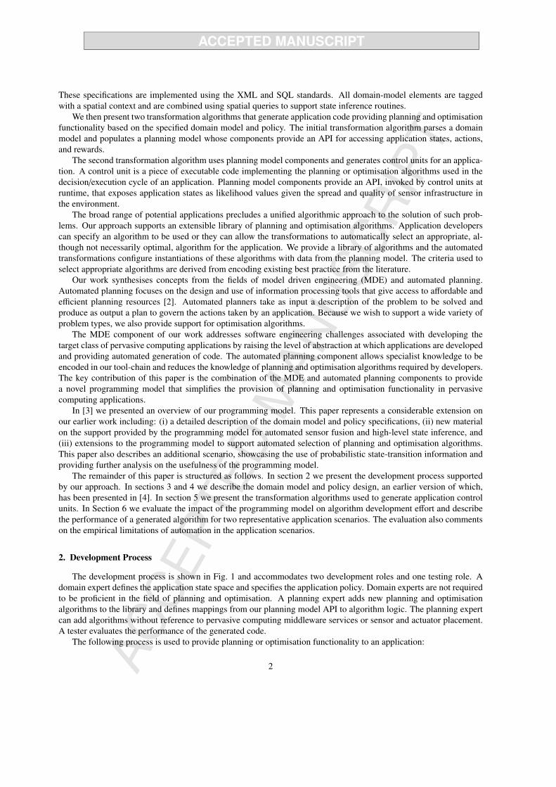
Layer 1 is used to specify infrastructural elements that exist in the deployment environment. Infrastructural ele-ments characterise physical artefacts relevant to the application being developed. All layer 1 elements have a spatialattribute specified using the Location Reference class shown in Fig 2. It contains a referenceSystemID and a locationattribute. The first attribute identifies the coordinate reference system used. By specifying a reference system identi-fier it allows elements to be specified in a range of geographic data formats and to be used in the same domain model.The location attribute specifies the geometric shape associated with the entity. The location and geometry propertiesare specified using the Simple Features Specification for SQL (SFS) standard, which provides a well-defined andcommon way for applications to store and access feature data in relational or object-relational databases [13].

5

Model Element

type : intdataSourceID : int

Infrastructure Element Location Reference

referenceSystemID : intlocation : String

1 1

Figure 2: Domain model infrastructure layer design.

Model Element


Actuator Element

name : Stringmobile : boolean

Sensor Element

name : Stringmobile : boolean

Location Reference


Data

name : Stringcost : intconfidence : float

Action

id : Stringcost : intconfidence : floattransition : String

11..* 1

1..*1

0..1

11

11

Figure 3: Domain model sensor and actuator layer design.

Both scenarios share a common layer 1 that specifies the city’s static road network infrastructure specified asa series of signalised junctions connected by road links that allow traffic to flow from one junction to another. Astandard model is used to represent the road network based on the Paramics traffic simulator2, formatted using theSFS spatial data standard and stored in a PostgreSQL GIS database. There are 247 junction elements whose spatialattributes are represented as circles of radius 20 metres from junction centre points and 2800 road link elements whosespatial attributes are represented as multi-polygon geometries summing the geometries of road links. Layer 1 datawas obtained from a Paramics model of Dublin city.

3.4. Layer 2

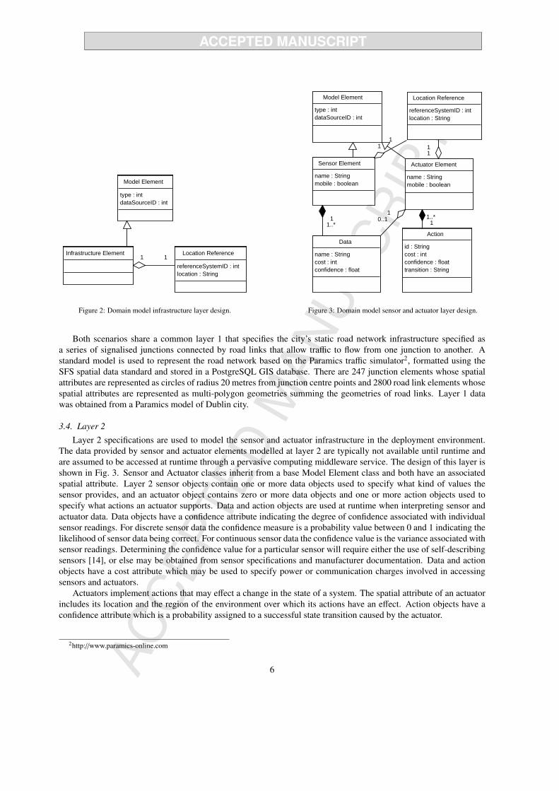
Layer 2 specifications are used to model the sensor and actuator infrastructure in the deployment environment.The data provided by sensor and actuator elements modelled at layer 2 are typically not available until runtime andare assumed to be accessed at runtime through a pervasive computing middleware service. The design of this layer isshown in Fig. 3. Sensor and Actuator classes inherit from a base Model Element class and both have an associatedspatial attribute. Layer 2 sensor objects contain one or more data objects used to specify what kind of values thesensor provides, and an actuator object contains zero or more data objects and one or more action objects used tospecify what actions an actuator supports. Data and action objects are used at runtime when interpreting sensor andactuator data. Data objects have a confidence attribute indicating the degree of confidence associated with individualsensor readings. For discrete sensor data the confidence measure is a probability value between 0 and 1 indicating thelikelihood of sensor data being correct. For continuous sensor data the confidence value is the variance associated withsensor readings. Determining the confidence value for a particular sensor will require either the use of self-describingsensors [14], or else may be obtained from sensor specifications and manufacturer documentation. Data and actionobjects have a cost attribute which may be used to specify power or communication charges involved in accessingsensors and actuators.

Actuators implement actions that may effect a change in the state of a system. The spatial attribute of an actuatorincludes its location and the region of the environment over which its actions have an effect. Action objects have aconfidence attribute which is a probability assigned to a successful state transition caused by the actuator.

2http://www.paramics-online.com

6

INSERT INTO s e n s o r ( id , d a t a S o u r c e I d , c o n f i d e n c e , name , da t a , c o s t , mobi l e )VALUES( ’ 247 ’ , ’ 2 ’ , ’ 0 . 8 5 ’ , ’ t r a f f i c d e m a n d ’ , ’ t r a f f i c d e m a n d ’ , ’ 1 ’ , ’ F a l s e ’ ) ;UPDATE s e n s o r SET geomet ry = GeomFromtext ( ’MULTIPOLYGON( ( ( 3 1 6 0 8 5 233921 ,316087.764019774

233927 .75649278 ,316109 .764019774. . . . . . . 316085 233921) ) ) ’ , −1) WHERE i d = ’ 247 ’ ;

Listing 1: Traffic-demand sensor meta-data specification excerpt.

��

��

��

��

��

��

��

��

��

��

��

Figure 4: Junction 1244 traffic phases and actions.

The effects of actions are specified using state charts. The domain model implementation uses a modified versionof the State Chart XML (SCXML) language, which specifies state transition information based on Harel State Tablesand which supports composite state spaces and probabilistic transitions [15], thus making it suitable for specifyingstate charts for pervasive computing environments.

Layer 2 of the CCTV Selection scenario domain model contains three sensor elements and one actuator element.An inductive loop sensor [16] provides sensor data on traffic demand and travel times. Weather station sensors aremodelled to provide data on rain fall levels at each junction. We also assume that a stationary pedestrian presence sen-sor is present at each junction to provide data on pedestrian levels. The spatial attribute of the weather and pedestriansensors is specified as an ellipse representing their sensing areas.

Listing 1 shows a traffic demand sensor entry in the domain model. The sensor has a confidence measure of 0.85which is interpreted as the likelihood P(tra f f ic demand == high|S ensorReading == high) = 0.85. A cost of 1 unitis associated with obtaining each sensor reading and the mobility flag is set to false. The spatial attribute of this sensoris specified as a multi-polygon shape, using an SFS function to convert a string of coordinates specified in the IrishNational Grid reference system, into a spatial geometry. Spatial data on fixed infrastructure is often available fromlocal authorities and through initiatives such as OpenStreetMap 3 which distribute spatial data freely.

Layer 2 for the Junction Controller scenario contains inductive loop sensors, emergency vehicle detection sensors,and traffic controller actuators located at each junction and responsible for switching traffic phases. The actionsspecified for each junction controller consists of the available traffic-control phases at that junction. An example ofthe set of actions available at Junction 1244 is shown in Fig 4(b). The actuator specification for Junction 1244 is shownin Listing 2. From Listing 2 actuator 1244 has a name which is the junction number and a mobility flag which is setto false and provides two actions: phase 1 and phase 2. Following SCXML terminology, these actions are describedusing state attributes. Each state attribute contains the following information:

• an id, which is the action name.

• the geometry or region over which the action is executed.

• each datamodel element contains a cost and confidence element indicating the cost of invoking this action onthe actuator and the likelihood of the action invocation succeeding.

3http://www.openstreetmap.org/

7

< a c t u a t o r><name>1244< / name><mobi le> f a l s e< / mobi le>< s t a t e>phase 1<geomet ry>MULTIPOLYGON( ( ( 3 1 6 2 8 0 233765316287019124818 233762994535766316265019124818

233685994535766316258 233688316280 233765) ) )< / geomet ry><da t amode l>< c o s t>1< / c o s t>< c o n f i d e n c e>0 .995< / c o n f i d e n c e>< !−− l i n k 1245−816 −−>< !−− l i n k 1245−1250 −−>

< / da t amode l>< t r a n s i t i o n e v e n t = ” swi t ch −phase 2 ” cond = ” rand l e s s e q 0 . 995 ” t a r g e t = ” phase 2 ” />< t r a n s i t i o n e v e n t = ” swi t ch − f a i l ” cond = ” ra nd g t 0 . 9 9 5 ” t a r g e t = ” f a i l ” />

< / s t a t e>. . . . . . . .

Listing 2: Excerpt of actuator specification for junction controller 1244.

• one or more transition elements indicating the state-action combinations to which the actuator can transitionand the likelihood of the transition succeeding.

An actuator record should be created to match every instance of a junction controller in the city.

3.5. Layer 3

Layer 3 of the domain model is used to specify the state-space of a pervasive computing application. Determiningstate values typically requires access to sensors and actuators distributed throughout the environment, the quality andspread of which will often be unknown at design time. Layer 3 system-state elements are used by domain experts tospecify the logic for calculating the values of application states, independently of run-time conditions. System-stateelements are composed using layer 1 and 2 elements to specify the types of sensor data and actuator actions, and thetypes of infrastructure in the deployment environment, that are required to calculate run-time values for the applicationstate space. Examples of system-states include vehicle throughput at a traffic junction, journey time along a road linkand power consumption in a room.

The design of this layer is shown in Fig. 5. Each system-state has a scope that indicates the region of the deploy-ment environment over which it is defined. Layer 1 and 2 elements referenced in a system-state definition are mappedat runtime onto matching physical entities in the region of the deployment environment described by the scope.

A system-state specification includes an inference function whose logic is used to calculate state values from therun-time values of sensor data and actuator actions. Sensor and actuator meta-data are used in the inference function toquantify the uncertainty associated with state values. Uncertainty is specified using discrete and continuous likelihoodfunctions for the true value of the system-state given the available sensor data.

System-state elements have a problemClass attribute indicating that the element belongs to either a planning or op-timisation problem. Deployment environment conditions are specified using dynamism, complexity, and observabilityattributes that are used to indicate respectively: that the state’s value can be affected by uncontrolled state-transitionevents; that it may be computationally difficult to compute the value of a system-state; and that the application statespace values are expressed as probabilities rather than direct observations. In the event that the domain expert doesnot specify which planning or optimisation algorithm to use, the transformations will use these four attributes to selectan appropriate planning or optimisation algorithm for the problem.

Layer 3 for the CCTV Selection scenario contains specifications of three system-states: JunctionInterest, Max-imalDistance, and DegreeofInterest. A JunctionInterest system-state is specified to be a monotonically increasingfunction of worsening weather conditions, pedestrian presence, and increasing traffic demand. Domain experts specifysystem-states in XML and the specification of the JunctionInterest system-state is shown in Listing 3. The dynamismand observability attributes are specified to be “true” and “partial” respectively, and the complexity attribute is setto “false”. The scope of the system-state is defined as being of type “element” and of value “junction”, meaning

8

Model Element


System-State Element

name : Stringdescription : StringsourceRef : URLproblemClass : Stringobservability : floatdynamism : booleancomplexity : booleanid : Integerscope : String

Data

name : Stringconfidence : float

Action

name : Stringconfidence : float

Infrastructure Element

Location Reference


11..*

1 0..*

1 0..*

1 1Inference Function

inferenceLogic : Stringvalue : floatconfidence : float

11

Figure 5: Domain model system-states layer design.

that a value for this system-state is to be calculated at each instance of a junction infrastructure element contained inthe scenario domain model. The implementation attribute contains a reference to an inference function that uses aBayesian network to combine the inputs to produce an output value for the system-state.

Figure 6: Bayesian network structure for JunctionInterest.

Rain

Mean 0.0

Variance 0.25

Traffic Volume

Low 0.2

Medium 0.4

High 0.4

Junction Interest

Pedestrians False True

Traffic Volume Low Medium High Low Medium High

Mean 1 3 5 3 5 7

Surface Water 5 5 5 5 5 5

Variance 2 2 2 2 2 2

Surface WaterMean 0.0

Rain 1.2

Variance 0.25

Figure 7: Bayesian network conditional probabilities for Junction-Interest.

Fig. 7 shows the conditional probability tables specified by the domain expert in the inference function. The hybridBayesian network contains a discrete Boolean Pedestrian node indicating whether pedestrians are present or not and adiscrete TrafficVolume node taking the values: “high”; “medium” and “low”. It also contains continuous SurfaceWa-ter, Rain and JunctionInterest nodes. A sample conditional probability from Fig. 7 reads P(S ur f aceWater|Rain) =

N(1.2 × Rain, 0.25), i.e., the continuous variable SurfaceWater has a mean value that is 20% higher than the valuesreported by the Rain sensor and a constant variance of 0.25. Such a specification might reflect the belief of the domainexpert that the rain sensors in general underestimate the amount of surface water by 20%.

A MaximalDistance system-state is defined to measure the geographic spread of the candidate set of CCTV cam-eras. To measure the geographic spread, sets of 30 selected cameras are modelled as nodes in a fully connectednetwork. The length of all network edges (distance between junctions) is measured in metres to obtain the total lengthof the network and used as a measure of coverage. This state is specified to be complex, static and fully observable asthe complexity of an exhaustive search of this space is O(cn) where n is the number of nodes and c > 1.

9

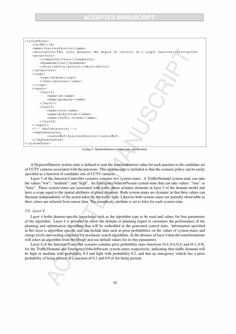
< s y s t e m S t a t e>001<name> J u n c t i o n I n t e r e s t< / name>< d e s c r i p t i o n>Thi s s t a t e measu res t h e d e g r e e o f i n t e r e s t o f a s i n g l e J u n c t i o n< / d e s c r i p t i o n>

<c o m p l e x i t y> f a l s e< / c o m p l e x i t y><dynamism> t r u e< / dynamism>< o b s e r v a b i l i t y> p a r t i a l< / o b s e r v a b i l i t y>

<scope>

< t y p e>e l e m e n t< / t y p e><v a l u e> j u n c t i o n< / v a l u e>

< / scope>

< l a y e r 1><name> i d< / name><name>geomet ry< / name>

< / l a y e r 1>< l a y e r 2>

<name> r a i n< / name><name> p e d e s t r i a n s< / name><name> t r a f f i c v o l u m e< / name>

< / l a y e r 2>< !−− I m p l e m e n t a t i o n s −−>

< s o u r c e R e f> J u n c t i o n I n t e r e s t< / s o u r c e R e f>

< / s y s t e m S t a t e>

Listing 3: JunctionInterest system-state specification.

A DegreeofInterest system-state is defined to sum the JunctionInterest value for each junction in the candidate setof CCTV cameras associated with the junctions. This system-state is included so that the scenario policy can be easilyspecified as a function of candidate sets of CCTV cameras.

Layer 3 of the Junction Controller scenario contains two system-states. A TrafficDemand system-state can takethe values:“low”; “medium”; and “high”. An EmergencyVehiclePresent system-state that can take values: “true” or“false”. These system-states are associated with traffic phase actuator elements in layer 2 of the domain model andhave a scope equal to the spatial attributes of phase elements. Both system-states are dynamic in that their values canfluctuate independently of the action taken by the traffic light. Likewise both system-states are partially observable astheir values are inferred from sensor data. The complexity attribute is set to false for each system-state.

3.6. Layer 4

Layer 4 holds domain-specific knowledge such as the algorithm type to be used and values for free parametersof the algorithm. Layer 4 is provided to allow the domain or planning expert to customise the performance of theplanning and optimisation algorithms that will be embedded in the generated control units. Information specifiedat this layer is algorithm specific and can include data such as prior probabilities on the values of system-states andenergy levels and cooling schedules for stochastic search algorithms. In the absence of layer 4 data the transformationswill select an algorithm from the library and use default values for its free parameters.

Layer 4 of the Junction Controller scenario contains prior probability mass functions (0.4, 0.4, 0.2) and (0.1, 0.9).for the TrafficDemand and EmergencyVehiclePresent system-states respectively, indicating that traffic demand willbe high or medium with probability 0.4 and light with probability 0.2, and that an emergency vehicle has a priorprobability of being present at a junction of 0.1 and 0.9 of not being present.

10

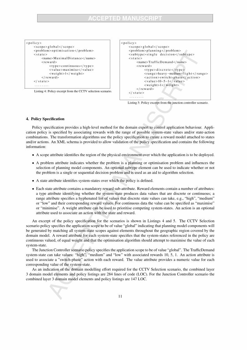
<scope>g l o b a l< / scope><problem> o p t i m i s a t i o n< / problem>< s t a t e>

<name>MaximalDis t ance< / name>< r eward>

< t y p e> c o n t i n u o u s< / t y p e><v a l u e>maximise< / v a l u e><w e ig h t>1< / we i g h t>

< / r eward>< / s t a t e>. . . . . . . .

Listing 4: Policy excerpt from the CCTV selection scenario.

<scope>g l o b a l< / scope><problem>p l a n n i n g< / problem>< s u b t y p e> s i n g l e d e c i s i o n< / s u b t y p e>< s t a t e>

<name>Traf f i cDemand< / name>< r eward>

< t y p e> d i s c r e t e< / t y p e>< r a n g e>heavy−medium− l i g h t< / r a n g e>< a c t i o n>swi t ch −phase< / a c t i o n><v a l u e>10−5−1< / v a l u e><w e i g h t>1< / w e i g h t>

< / r eward>< / s t a t e>. . . . . . . .

Listing 5: Policy excerpt from the junction controller scenario.

4. Policy Specification

Policy specification provides a high-level method for the domain expert to control application behaviour. Appli-cation policy is specified by associating rewards with the range of possible system-state values and/or state-actioncombinations. The transformation algorithms use the policy specification to create a reward model attached to statesand/or actions. An XML schema is provided to allow validation of the policy specification and contains the followinginformation:

• A scope attribute identifies the region of the physical environment over which the application is to be deployed.

• A problem attribute indicates whether the problem is a planning or optimisation problem and influences theselection of planning model components. An optional subtype element can be used to indicate whether or notthe problem is a single or sequential decision problem and is used as an aid to algorithm selection.

• A state attribute identifies system-states over which the policy is defined.

• Each state attribute contains a mandatory reward sub-attribute. Reward elements contain a number of attributes:a type attribute identifying whether the system-state produces data values that are discrete or continuous; arange attribute specifies a hyphenated list of values that discrete state values can take, e.g., “high”, “medium”or “low” and their corresponding reward values. For continuous data the value can be specified as “maximise”or “minimise”. A weight attribute can be used to prioritise competing system-states. An action is an optionalattribute used to associate an action with the state and reward.

An excerpt of the policy specification for the scenarios is shown in Listings 4 and 5. The CCTV Selectionscenario policy specifies the application scope to be of value “global” indicating that planning model components willbe generated by matching all system-state scopes against elements throughout the geographic region covered by thedomain model. A reward attribute for each system-state specifies that the system-states referenced in the policy arecontinuous valued, of equal weight and that the optimisation algorithm should attempt to maximise the value of eachsystem-state.

The Junction Controller scenario policy specifies the application scope to be of value “global”. The TrafficDemandsystem-state can take values: “high”, “medium” and “low” with associated rewards 10, 5, 1. An action attribute isused to associate a ”switch-phase” action with each reward. The value attribute provides a numeric value for eachcorresponding value of the system-state.

As an indication of the domain modelling effort required for the CCTV Selection scenario, the combined layer3 domain model elements and policy listings are 284 lines of code (LOC). For the Junction Controller scenario thecombined layer 3 domain model elements and policy listings are 147 LOC.

11

5. Model Transformations

The model transformations produce application code that executes over an assumed middleware to provide thedesired planning and optimisation behaviour as expressed in the domain model and policy. The first transformationextracts information from the domain model to populate planning model components that provide a programminginterface to pervasive computing environments modelled on a five-tuple

∑= (S , A,T,O,R) where:

• S = {s1, s2, ..} is the set of system states;

• A = {a1, a2, ..} is the set of actions provided by actuator functionality;

• T (s, a, s′) represents a stochastic state-transition function that gives the probability P(s

′ |s, a) of moving to states′

if the action a is performed in state s.

• O = {o1, o2, ..} is the set of observations that are produced by the sensor infrastructure in the region. Anobservation or sensor model function O(s

′, a, o) gives the probability P(o|a, s′ ) of observing o if action a is

performed and the resulting state is s′.

• R(s, a, s′) represents the immediate reward for performing action a while in state s and moving to state s

′.

Application state is represented as variables that provide estimates of changing value and certainty at runtime.From

∑, each si ∈ S represents a system-state element that is implemented by a set of state-variable objects.

State-variable objects are planning model components, generated by the transformations using domain model system-state specifications, to perform sensor fusion and state inference services. They perform the sensor model functionO(s

′, a, o), by combining spatial attributes with named layer 2 sensor data and actuator action inputs, to invoke mid-

dleware services and return the run-time values of system-states in the deployment environment. The number ofstate-variable objects required for each system-state is calculated using the system-state and policy scope information.For example, if a system-state has a scope of type “element”, a state-variable object is created for each matchingelement within the policy scope.

Actuator objects are generated from layer 2 elements to provide an interface to actions and associated state-transitions currently specified in SCXML. Support for additional state-transition formats such as dynamic Bayesiannetworks (DBNs) could be added by extending the domain model transformation to compile the DBN format into theinternal representation for state-transition systems used in the planning model.

Reward model entries R(s, a, s′) are implemented as a multi-dimensional hash-table containing tables indexed by

each system-state name in the domain model. For discrete states, numeric rewards are stored for state/action combi-nations extracted from the policy specified by the domain expert. Continuous states are indexed with maximisation orminimisation tag values.

5.1. Domain Model To Planning Model Transformation

The logic of this first transformation is summarised under the following three headings:

1. Parse the policy and system-state specifications.The policy file and system-state specifications are validated using their respective schemas. The policy scopeindicates the extent of the region over which the application is to be deployed. The problem type will be eitherplanning or optimisation and determines the required planning model components. The scope, complexity,dynamism and observability properties are recorded for each system-state. The set of layer 1, 2 and 3 inputs areread for each system-state and a reference to the state inference function is recorded.

2. Planning problems.The set of state-variable objects for each system-state are enumerated and instantiated. Layer 2 meta-data isread and used to create spatial queries that are written into the sets of state-variable objects. Actuator elementsspecified in layer 2 of the domain model are validated and a set of actuator objects created, containing specifiedtransition system information and action confidence values. A reward model is built using the reward elementscontained in the policy.

12

3. Optimisation problems.For complex optimisation problems the state space will often be too large to evaluate fully and the overheadof creating a full set of state-variable objects is impractical. For example, in the CCTV Selection scenario,there are 247!

(247−30)! permutations of 30 CCTV installations that can be chosen from the 247 available. Heuris-tic optimisation algorithms manage complexity by exploring random subsets of an application state space. Toaccommodate random exploration of complex pervasive computing state-spaces, the domain-model transfor-mation creates state-generator factories used by optimisation algorithms to produce state-variable objects withrandomly chosen spatial attributes on demand at runtime. State-variable objects generated for optimisationproblems are functionally identical to those used in planning problems.

5.2. Planning Model Sensor Fusion Support

State-variable objects combine their spatial attributes with layer 2 input names and perform sensor and actuatorlookup and access operations by invoking middleware services. By default state-variable objects perform low-levelautomated competitive fusion of sensor data. Competitive sensor fusion techniques are employed when multiplesensors deliver independent measures of the same property and use weighted average algorithms to reduce the effectsof uncertain and erroneous measurements [17].

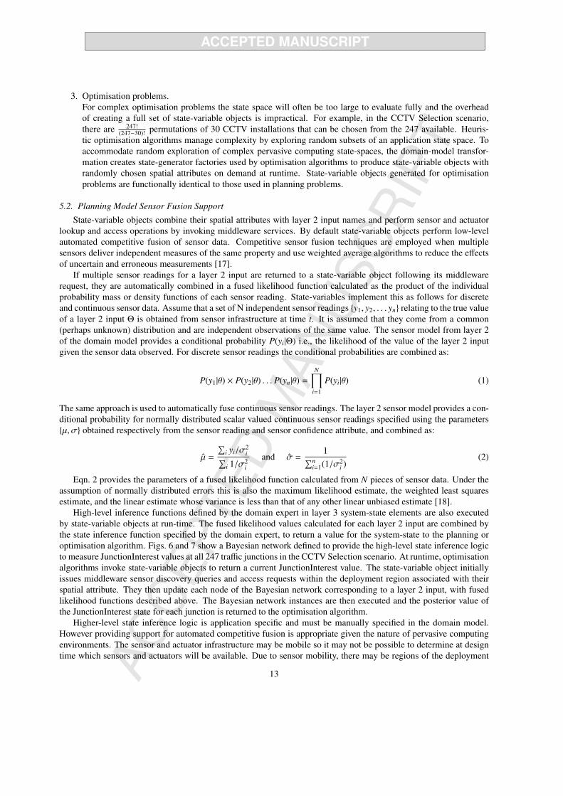
If multiple sensor readings for a layer 2 input are returned to a state-variable object following its middlewarerequest, they are automatically combined in a fused likelihood function calculated as the product of the individualprobability mass or density functions of each sensor reading. State-variables implement this as follows for discreteand continuous sensor data. Assume that a set of N independent sensor readings {y1, y2, . . . yn} relating to the true valueof a layer 2 input Θ is obtained from sensor infrastructure at time t. It is assumed that they come from a common(perhaps unknown) distribution and are independent observations of the same value. The sensor model from layer 2of the domain model provides a conditional probability P(yi|Θ) i.e., the likelihood of the value of the layer 2 inputgiven the sensor data observed. For discrete sensor readings the conditional probabilities are combined as:

P(y1|θ) × P(y2|θ) . . . P(yn|θ) =

N∏

i=1

P(yi|θ) (1)

The same approach is used to automatically fuse continuous sensor readings. The layer 2 sensor model provides a con-ditional probability for normally distributed scalar valued continuous sensor readings specified using the parameters{µ, σ} obtained respectively from the sensor reading and sensor confidence attribute, and combined as:

µ =

∑i yi/σ

2i∑

i 1/σ2i

and σ =1∑n

i=1(1/σ2i )

(2)

Eqn. 2 provides the parameters of a fused likelihood function calculated from N pieces of sensor data. Under theassumption of normally distributed errors this is also the maximum likelihood estimate, the weighted least squaresestimate, and the linear estimate whose variance is less than that of any other linear unbiased estimate [18].

High-level inference functions defined by the domain expert in layer 3 system-state elements are also executedby state-variable objects at run-time. The fused likelihood values calculated for each layer 2 input are combined bythe state inference function specified by the domain expert, to return a value for the system-state to the planning oroptimisation algorithm. Figs. 6 and 7 show a Bayesian network defined to provide the high-level state inference logicto measure JunctionInterest values at all 247 traffic junctions in the CCTV Selection scenario. At runtime, optimisationalgorithms invoke state-variable objects to return a current JunctionInterest value. The state-variable object initiallyissues middleware sensor discovery queries and access requests within the deployment region associated with theirspatial attribute. They then update each node of the Bayesian network corresponding to a layer 2 input, with fusedlikelihood functions described above. The Bayesian network instances are then executed and the posterior value ofthe JunctionInterest state for each junction is returned to the optimisation algorithm.

Higher-level state inference logic is application specific and must be manually specified in the domain model.However providing support for automated competitive fusion is appropriate given the nature of pervasive computingenvironments. The sensor and actuator infrastructure may be mobile so it may not be possible to determine at designtime which sensors and actuators will be available. Due to sensor mobility, there may be regions of the deployment

13

environment with a proliferation of sensors and other regions with few or no sensors. A region with many sensorsproviding data for the same state input should have a lower uncertainty than a region with less sensor data. Automatedcompetitive fusion allows varying levels of sensor coverage to be exploited by planning and optimisation algorithmsat runtime.

5.3. Planning Model To Control Unit Transformation

The logic of this second transformation is summarised under the following two headings:

1. Read algorithm selection logic and problem type.The algorithm library is validated using the library XSD schema. Information indexing the available algorithmsby problem type and environment properties is read from the algorithm taxonomy. The problem, complexity,observability, and dynamism attributes are read for each system-state contained in the planning model.

2. Algorithm selection and control unit instantiation.The problem and subtype attributes in system-state templates are used to identify the root branch of the algo-rithm taxonomy and the domain characteristics are used to select a particular algorithm. The algorithm compo-nents are then mapped to the planning model components and control units are instantiated using the templatesshown in Algs. 1 and 2. Algorithms selected automatically are assigned default values for free parameters,specified by the planning expert when the algorithm is added to the library.

5.3.1. Algorithm SelectionTable 1 lists the library of algorithms we provide for inference, planning, and optimisation problems. The first

column of each section lists the problem type. The second column shows the type of algorithm and the third columnlists the system-state properties deemed relevant to selecting an algorithm. The fourth column lists the algorithmsprovided for a combination of problem and system-state properties.

The planning expert can implement multiple algorithms for each problem type and property set and can specifywhich algorithm to use in the domain model. However if automatic algorithm selection is used then only algorithmsreferenced in the taxonomy are considered for selection. The algorithms available for automatic selection are shownin bold print in Table 1.

The taxonomy specifies that competitive inference problems are implemented with a weighted average mean algo-rithm in partially observable environments. Feature/decision-level state inference problems are currently implementedusing a Bayesian network library that has been integrated into the algorithm library.

Domain experts may not be familiar with Bayesian networks and may choose to use another high-level inferencetechnique. The planning model interface exposes state values as likelihood functions to planning and optimisationalgorithms. Additional state inference techniques providing likelihood functions for application state can be added tothe library without impacting the planning and optimisation algorithms contained in the algorithm library.

Single decision problems are modelled using the principle of maximum expected utility and implemented us-ing Bayesian decision networks. Sequential decision planning problems are implemented using a Markov DecisionProcess (MDP) framework [2]. If the environment is partially observable and dynamic, then an online approximatePOMDP algorithm is chosen. The POMDP framework supports a wide range of exact and approximate, online andoffline approaches to planning [19]. Solutions to optimisation problems are based on heuristic algorithms. If theenvironment is dynamic a stochastic approximation algorithm is chosen. For applications with complex state spaces,a simulated annealing algorithm is chosen. The association of problem type to algorithm selection is informed byreference to the literature and can be amended by editing the taxonomy.

5.3.2. Control Unit TemplatesThe execution cycle of a control unit for a planning problem is shown in Alg. 1. In lines 1-3 each state-variable

object in the planning model updates the application state values. Multiple sensor readings returned by middlewarelookup operations are automatically fused and passed into inference functions executed at runtime. In lines 5-6,the control unit uses the policy specified by the domain expert, and transformed into a reward model, to calculate theutility of invoking each available action given the updated state information. The action selection logic is implementedby the planning algorithm embedded within the control unit. For single-decision planning problems, the control unit

14

Inference Problems

Type Principle Properties AlgorithmCompetitive Fused Maximum Likelihood Estimate Partial-Observability Weighted-Average Mean

Feature & Decision Level Bayesian Inference Partial-Observability Bayesian Network

Planning Problems

Type Principle Properties Algorithm

Single Decision Maximum Expected Utility AllBayesian Decision Network

Random Action SelectionRound Robin

Sequential-Decision Markov Decision Process (MDP) Partial-Observability POMDPSequential-Decision MDP Dynamism Online POMDPSequential-Decision MDP Complexity Online Approx POMDP

Optimisation Problems

Optimisation Stochastic Search Dynamism Local SearchOptimisation Stochastic Search Dynamism & Complexity Simulated Annealing

Table 1: Algorithm library and taxonomy

returns the action that maximises the reward at each time step. For sequential planning problems the control unitselects an action that maximises the reward over a planning horizon.

Alg. 2 shows the execution cycle of a control unit for an optimisation problem. A collection of state-variableobjects evaluated by an optimisation algorithm is referred to as a candidate solution. In line 1, a candidate solutionθ, from the domain of possible solutions Θ, is initially generated subject to the system-state specifications. Heuris-tic optimisation algorithms generate initial candidate solutions stochastically. Lines 3-5, invoke the state inferencefunctions provided by state-variable objects to obtain values for candidate solutions. In line 8, the control units useL(θ), a loss function generated from the policy specified by the domain expert to evaluate the candidate. The logicgoverning candidate generation and evaluation is specific to the optimisation algorithm contained within the controlunit. The stopping criterion tested in line 2 and the generation of new candidate solutions in line 10 are also specificto the optimisation algorithm contained within the control unit.

5.4. Scenario Transformations

The CCTV Selection scenario is specified in Listing 4 to be an optimisation problem. The domain-model trans-formation populates the planning model components to provide a state-generator factory and a reward model fromthe policy and system-state specifications At runtime, 30 state-variable objects associated with the JunctionInterestsystem-state query for sensor data, compute a fused likelihood function for each layer 2 input and then enter thelikelihood data into the Bayesian network specified by the domain expert. The mean value returned by 30 Bayesiannetworks representing candidate sets of 30 junctions are summed by DegreeofInterest state-variable objects. TheMaximalDistance state-variable objects calculate the geographic spread of the candidate set of 30 junctions.

The algorithm taxonomy currently specifies that a simulated annealing algorithm based on the SMOSA algorithm[20] is preferred for optimisation problems with complex, partially-observable and dynamic state spaces. The SMOSAalgorithm supports multi-objective problems and generates solutions that are optimal in the sense that no other solu-tions in the search space are superior to each other when the two objectives are considered. Such solutions are knownas Pareto-optimal [20].

In line 1 of Alg 2, a candidate solution set θ of 30 CCTV cameras, from the 247!(247−30)! possible solutions is generated.

In lines 2-5, sensor data and inference functions are used to calculate DegreeofInterest and MaximalDistance valuesfor θ. The SMOSA algorithm works by randomly selecting and evaluating a neighbour s

′of the current state s, and

probabilistically accepting or rejecting s′

as the new state. The transition or acceptance probabilities are controlled bya temperature parameter T and adapted throughout the process so that the system can avoid local minima and tends

15

Algorithm 1: Planning problem control unittemplate.

Input:∑

: a planning model; Alg: an instanceof a planning algorithm.

foreach si ∈ S do1

integrate sensor evidence into si;2

calculate P′(si);3

end4

foreach action ai ∈ A do5

calculate Alg(ai, s′i), the reward for taking6

action A;end7

return the best action from A;8

Algorithm 2: Optimisation problem controlunit template.

Input:∑

: a planning model; Alg: an instanceof an optimisation algorithm.

generate candidate set(s) {S (θ) ∈ Θ};1

while not finished do2

foreach θ ∈ S (θ) do3

integrate sensor evidence into θ ;4

calculate P′(θ);5

end6

foreach θ ∈ S (θ) do7

evaluate the loss function L(θ) ;8

end9

generate new candidate set(s) {S (θ) ∈ Θ};10

end11

return the best solution from S (θ);12

to move to states of lower energy [20]. The number of evaluation iterations performed by the SMOSA algorithm iscontrolled through a run-count parameter.

The utility of solutions found by the SMOSA algorithm are dynamic due to fluctuating traffic volumes, weatherchanges and pedestrian presence. The control unit should be re-run periodically to generate solutions in a dynamicenvironment. The planning expert can use layer 4 of the domain model to specify a range of possible values forthe temperature and run-count parameters. Our tool-chain can be used by planning experts to empirically assessappropriate algorithms and parameters for applications.

The Junction Controller scenario is specified in Listing 5 to be a single-decision planning problem and the al-gorithm taxonomy specifies that Bayesian decision networks are used to implement control units for this class ofproblem. Decision networks are an extension of Bayesian networks to incorporate actions and utilities and provide acompact model for single-decision processes [21]. Given a stochastic transition function and some sensor evidenceE, actions are selected to maximise the expected utility (MEU), calculated as [22]:

EU(a | E) =∑

s′P(s, a, s

′, | e) U(s

′) (3)

The planning-model transformation instantiates a template decision network at each junction controller actuator.The transformation algorithm obtains the decision network structure as follows: initially a chance (oval) node iscreated for each system-state template object which can be discrete or continuous depending on the system-statedata type, subsequently decision nodes (rectangle) are created for actions supported by the actuator functionality,and finally a utility node (diamond) is created and configured with reward model data combined using an additiveutility function and shown in in Table 2. The structure of the decision networks generated by the planning-modeltransformation for the Junction Controller scenario control units is shown in Fig. 8. The transformation algorithmthen searches layer 4 data to find prior probabilities specified by the domain expert for system-states related to chancenodes.

The scenario domain model contains 247 junction actuator records and a decision network is generated for eachone using the planning problem control unit template. As the control units execute they calculate the posterior valueof each chance node given the available run-time evidence derived from sensor and actuator data. Alg. 3 shows thelogic used to map chance nodes to state-variable objects. The evidence is generated by state-variable objects andreturned to the control unit as likelihood functions, where it is mapped to the corresponding chance nodes in each ofthe 247 decision networks. Once the posterior probabilities are calculated for chance nodes, the utility of each actionis calculated and the action with the highest utility is returned. This cycle continues until the control units are halted.

16

Reward Switch TrafficDemand EmergencyVehiclePresent index10 Switch=Change TrafficDemand=high EmergencyVehiclePresent=false 040 Switch=Change TrafficDemand=high EmergencyVehiclePresent=true 15 Switch=Change TrafficDemand=medium EmergencyVehiclePresent=false 2

35 Switch=Change TrafficDemand=medium EmergencyVehiclePresent=true 31 Switch=Change TrafficDemand=low EmergencyVehiclePresent=false 4

31 Switch=Change TrafficDemand=low EmergencyVehiclePresent=true 5

Table 2: Junction Controller decision network reward model.

Algorithm 3: Adding evidence to a decisionnetwork.

Input: A: action; DN: a Decision Network.foreach chance node ∈ DN do1

lookup an associated state-variable in2

action scope;read the likelihood function over the3

state-variable value;enter likelihood evidence into the chance4

node;end5

compute the posterior probabilities across the6

network;

��

��

Figure 8: A decision network generated to run a traffic junctioncontroller.

6. Evaluation

This paper presents a development process incorporating concepts from the domains of model-driven engineeringand automated planning. We present an empirical evaluation of the impact of our tool chain on the effort of developingthe scenarios and a quantitative evaluation of the performance of the planning and optimisation algorithms generatedby the automated-planning component for the scenarios. This section is structured as follows. The evaluation met-rics used for development effort and algorithm performance are introduced. These metrics are then applied to thetwo evaluation scenarios. Finally we discuss the implications of our results for automating the use of planning andoptimisation algorithms in pervasive computing applications.

6.1. Evaluation Metrics

The following approach was used to measure the impact of the development process on reducing the developmenteffort for applying planning and optimisation algorithms in pervasive computing environments. The lines of code(LOC) provided by the domain and planning expert for each scenario were recorded. The size of the spatial queryset produced by the automated transformations was recorded and used as a proxy measure for the development effortprovided by the transformation engine. The scenarios were then extended by adding new requirements and the LOCmetric measured for the extended domain and planning expert development (DM and PL respectively). The transfor-mations were re-run and the increase in size of the spatial query data produced recorded. The ratio of increased domainand planning development effort in LOC was then compared to the ratio of the increase in spatial query data generated.This value is referred to as the “degree of automation” and calculated as: δ(DM + PL) / δ(Planning Model S ize).

We are interested in algorithm performance insofar as it can be used to judge the efficacy of our developmentprocess and tool chain. Accordingly we evaluate algorithm performance to show that the generated code is functionaland behaves in accordance with the policy. We also evaluate automated algorithm selection by comparing the perfor-mance of the automatically selected algorithms relative to a chosen baseline algorithm. Applying multiple algorithmsto a common domain model demonstrates that model and algorithm reuse is supported by the methodology. Finallywe investigate the impact of control tuning by evaluating how algorithm performance is impacted by tuning parametervalues.

17

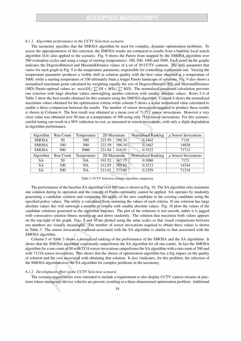
6.1.1. Algorithm performance in the CCTV Selection scenarioThe taxonomy specifies that the SMOSA algorithm be used for complex, dynamic optimisation problems. To

assess the appropriateness of this selection, the SMOSA results are compared to results from a baseline local searchalgorithm (SA) also applied to the scenario. Fig. 9 shows the Pareto front mapped by the SMOSA algorithm over500 evaluation cycles and using a range of starting temperatures: 100, 500, 1000 and 5000. Each point on the graphsindicates the DegreeofInterest and MaximalDistance values of a set of 30 CCTV cameras. The only parameter thatvaries for each graph in Fig. 9 is the temperature parameter, responsible for controlling exploration rate. Varying thetemperature parameter produces a visible shift in solution quality with the best value obtained at a temperature of5000, while a starting temperature of 100 ultimately finds a longer Pareto landscape of solutions. Fig. 9 also shows anormalised maximum point calculated by weighting equally the sets of DegreeofInterest (DI) and MaximalDistance(MD) Pareto-optimal values as: max{DIi/

∑ni DI + MDi/

∑ni MD}. The normalised maximum calculation prevents

one criterion with large absolute values outweighing another criterion with smaller absolute values. Rows 2-4 ofTable 3 show the best results obtained for this scenario using the SMOSA algorithm. Column 4 shows the normalisedmaximum values obtained for the optimisation criteria while column 5 shows a scalar normalised value calculated toenable a direct comparison between the results. The number of sensor invocations required to produce these resultsis shown in Column 6. The best result was obtained at a mean cost of 71,712 sensor invocations. However a veryclose value was obtained over 50 runs at a temperature of 500 using only 7118 sensor invocations. For this scenario,careful tuning can result in a 90% reduction in cost, as measured in sensor invocations, with only a slight degradationin algorithm performance.

Algorithm Run Count Temperature 2D Maximum Normalised Ranking µ Sensor InvocationsSMOSA 50 500 223.59 398.34 0.3462 7118SMOSA 100 500 223.59 398.34 0.3462 14028SMOSA 500 5000 221.04 416.91 0.3522 71712

Algorithm Run Count Temperature 2D Maximum Normalised Ranking µ Sensor InvocationsSA 50 NA 191.52 367.75 0.3080 7173SA 100 NA 212.95 359.82 0.3213 14344SA 500 NA 211.01 373.99 0.3259 71218

Table 3: CCTV Selection scenario algorithm comparison

The performance of the baseline SA algorithm over 500 runs is shown in Fig. 10. The SA algorithm only maintainsone solution during its operation and the concept of Pareto-optimality cannot be applied. SA operates by randomlygenerating a candidate solution and comparing the utility of the new candidate to the existing candidate using thespecified policy values. The utility is calculated from summing the values of each criteria. If one criterion has largeabsolute values this will outweigh a number or criteria with smaller absolute values. Fig. 10 plots the values of thecandidate solutions generated as the algorithm executes. The plot of the solutions is not smooth, rather it is jaggedwith consecutive solution fitness moving up and down randomly. The solution that maximise both values appearson the top-right of the graph. Figs. 9 and 10 are plotted using the same scales so that visual comparisons betweenrun numbers are visually meaningful. The number of sensor invocations required to obtain these values is shownin Table 3. The sensor invocation overhead associated with the SA algorithm is similar to that associated with theSMOSA algorithm.

Column 5 of Table 3 shows a normalised ranking of the performance of the SMOSA and the SA algorithms. Itshows that the SMOSA algorithm consistently outperforms the SA algorithm for all run counts. In fact the SMOSAalgorithm for a run count of 50 with 7118 sensor invocations outperforms the SA algorithm with a run count of 500 andwith 71218 sensor invocations. This shows that the choice of optimisation algorithm has a big impact on the qualityof solution and the cost associated with obtaining that solution. It also vindicates, for this problem, the selection ofthe SMOSA algorithm over the SA algorithm for complex problems in the taxonomy.

6.1.2. Development effort in the CCTV Selection scenarioThe scenario requirements were extended to include a requirement to also display CCTV camera streams at junc-

tions where emergency service vehicles are present, resulting in a three-dimensional optimisation problem. Additional

18

layer 3 system-states, EmergencyVehiclePresent and NumberEmergencyVehicles, were defined to detect and count thenumber of emergency service vehicles at junctions associated with selected sets of CCTV cameras. The addition ofthe system-states increase the domain model by 106 lines: 78 lines of XML and 28 lines of python. Of this increase,10 lines of XML are for the policy extensions, 68 lines of XML are for the system-state definitions and the 28 lines ofpython code are for the inference functions.

Specifying the additional functionality increased the size of the domain modelling effort by c. 40% from 284to 390 LOC. The SMOSA implementation and mapping was 400 LOC. However there was no additional planningdevelopment effort required as the SMOSA algorithm mapping logic is unchanged. The increase in development effortδ(DM + PL) was 684/790 LOC = 15%. The spatial query set generated by the transformation engine from the originaldomain model was 69 KB in size. This increased to 118KB in size for the extended domain model. The degree ofautomation measure for the extended scenario was: 684/790 : 69/118, i.e., a 15% increase in development effortwas translated by the tool-chain into a 71% increase in application functionality as measured by the size of generatedspatial query data. The increased functionality was mirrored in evaluation logs that show the original SMOSA controlunits performed 7118 sensor invocations over 50 runs while the extended SMOSA control units performed 8823sensor invocations over 50 runs, an increase of c. 24%.

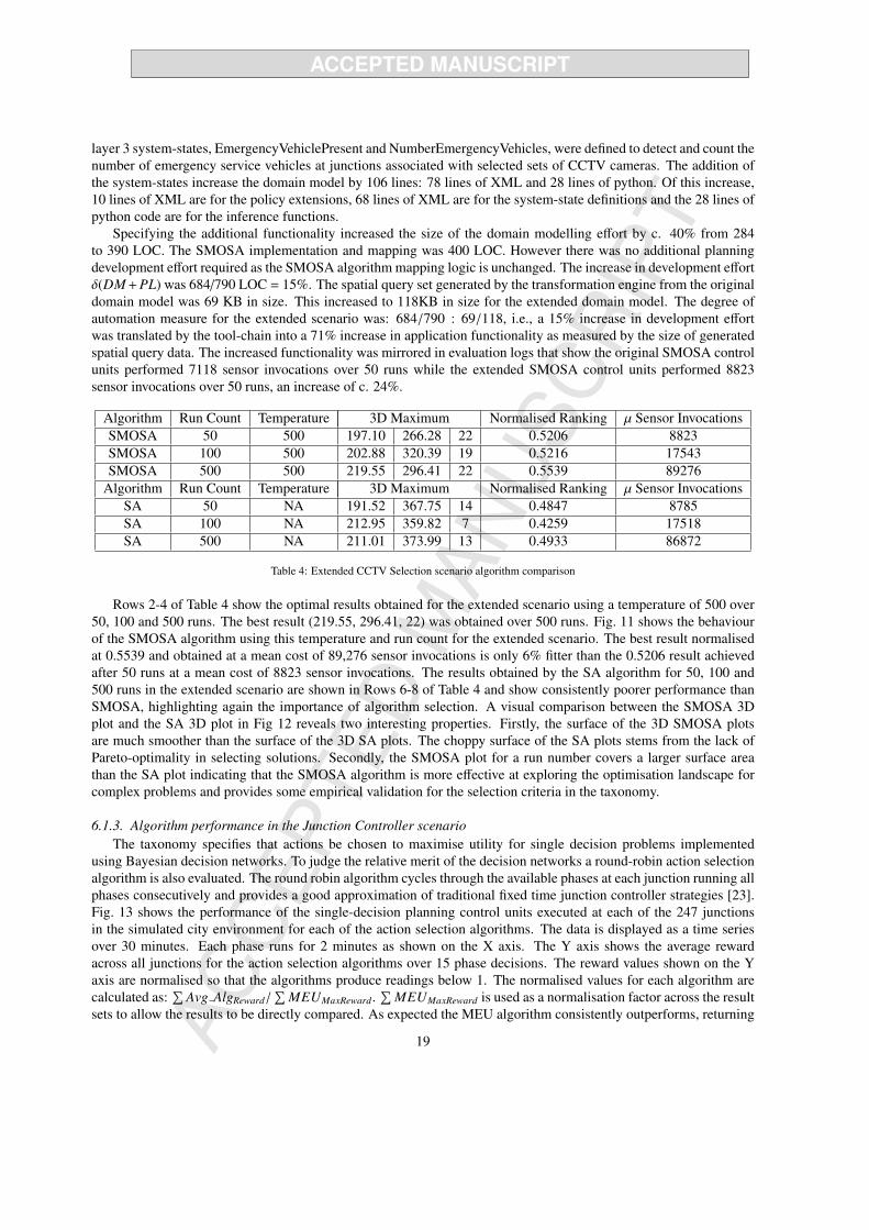
Algorithm Run Count Temperature 3D Maximum Normalised Ranking µ Sensor InvocationsSMOSA 50 500 197.10 266.28 22 0.5206 8823SMOSA 100 500 202.88 320.39 19 0.5216 17543SMOSA 500 500 219.55 296.41 22 0.5539 89276

Algorithm Run Count Temperature 3D Maximum Normalised Ranking µ Sensor InvocationsSA 50 NA 191.52 367.75 14 0.4847 8785SA 100 NA 212.95 359.82 7 0.4259 17518SA 500 NA 211.01 373.99 13 0.4933 86872

Table 4: Extended CCTV Selection scenario algorithm comparison

Rows 2-4 of Table 4 show the optimal results obtained for the extended scenario using a temperature of 500 over50, 100 and 500 runs. The best result (219.55, 296.41, 22) was obtained over 500 runs. Fig. 11 shows the behaviourof the SMOSA algorithm using this temperature and run count for the extended scenario. The best result normalisedat 0.5539 and obtained at a mean cost of 89,276 sensor invocations is only 6% fitter than the 0.5206 result achievedafter 50 runs at a mean cost of 8823 sensor invocations. The results obtained by the SA algorithm for 50, 100 and500 runs in the extended scenario are shown in Rows 6-8 of Table 4 and show consistently poorer performance thanSMOSA, highlighting again the importance of algorithm selection. A visual comparison between the SMOSA 3Dplot and the SA 3D plot in Fig 12 reveals two interesting properties. Firstly, the surface of the 3D SMOSA plotsare much smoother than the surface of the 3D SA plots. The choppy surface of the SA plots stems from the lack ofPareto-optimality in selecting solutions. Secondly, the SMOSA plot for a run number covers a larger surface areathan the SA plot indicating that the SMOSA algorithm is more effective at exploring the optimisation landscape forcomplex problems and provides some empirical validation for the selection criteria in the taxonomy.

6.1.3. Algorithm performance in the Junction Controller scenarioThe taxonomy specifies that actions be chosen to maximise utility for single decision problems implemented

using Bayesian decision networks. To judge the relative merit of the decision networks a round-robin action selectionalgorithm is also evaluated. The round robin algorithm cycles through the available phases at each junction running allphases consecutively and provides a good approximation of traditional fixed time junction controller strategies [23].Fig. 13 shows the performance of the single-decision planning control units executed at each of the 247 junctionsin the simulated city environment for each of the action selection algorithms. The data is displayed as a time seriesover 30 minutes. Each phase runs for 2 minutes as shown on the X axis. The Y axis shows the average rewardacross all junctions for the action selection algorithms over 15 phase decisions. The reward values shown on the Yaxis are normalised so that the algorithms produce readings below 1. The normalised values for each algorithm arecalculated as:

∑Avg AlgReward/

∑MEUMaxReward.

∑MEUMaxReward is used as a normalisation factor across the result

sets to allow the results to be directly compared. As expected the MEU algorithm consistently outperforms, returning

19

320

340

360

380

400

420

440

140 160 180 200 220 240

Max

imal

Dis

tanc

e in

km

s

Degree of Interest

’500r_100t’’500r_500t’

’500r_1000t’’500r_5000t’

"normalised_max"

Figure 9: CCTV Selection - SMOSA performance for 500 runs.

280

300

320

340

360

380

400

420

440

140 160 180 200 220 240

Max

imal

Dis

tanc

e in

km

s

Degree of Interest

’plot500r’ using 2:1"max" using 2:1

Figure 10: CCTV Selection - SA performance for 500 runs.

140

160

180

200

220 260

280 300

320 340

360 380

400 420

8 10 12 14 16 18 20 22 24

Num

ber

of E

mer

genc

y V

ehic

les

"500r_500t""normalised_max"

Degree of Interest

Maximal Distance in kms

8 10 12 14 16 18 20 22 24

Figure 11: CCTV Selection ext. - SMOSA performance for 500runs.

120

140

160

180

200

220 240

260 280

300 320

340 360

380 400

420

8 10 12 14 16 18 20 22 24

Num

ber

of E

mer

genc

y V

ehic

les

"500r" using 2:1:3"max" using 2:1:3

Degree of Interest

Maximal Distance in kms

6 8 10 12 14 16 18 20 22

Figure 12: CCTV Selection ext. - SA performance for 500 runs.

0.85

0.9

0.95

1

1.05

1.1

1.15

1.2

00:00 03:00 06:00 09:00 12:00 15:00 18:00 21:00 24:00 27:00 30:00

Util

ity

Time in Minutes

MEURound Robin

Figure 13: Junction Controller control unit performance.

0.85

0.9

0.95

1

1.05

1.1

1.15

1.2

00:00 03:00 06:00 09:00 12:00 15:00 18:00 21:00 24:00 27:00 30:00

Util

ity

Time in Minutes

MEURound Robin

Figure 14: Extended Junction Controller control unit performance.

20

0

500

1000

1500

2000

2500

3000

3500

App

licat

ion

Cod

e S

ize

in L

OC

147 207284

390 420 400

1760

2931

Junction Controller DMJunction Controller DM Ext.

CCTV Selection DM CCTV Selection DM Ext.

Junction Controller AICCTV selection AI

TransformationsInference

Figure 15: LOC effort to implement the Junction Controller andCCTV Selection scenarios.

��

��

��

Figure 16: The extended Bayesian decision network for junctioncontrollers.

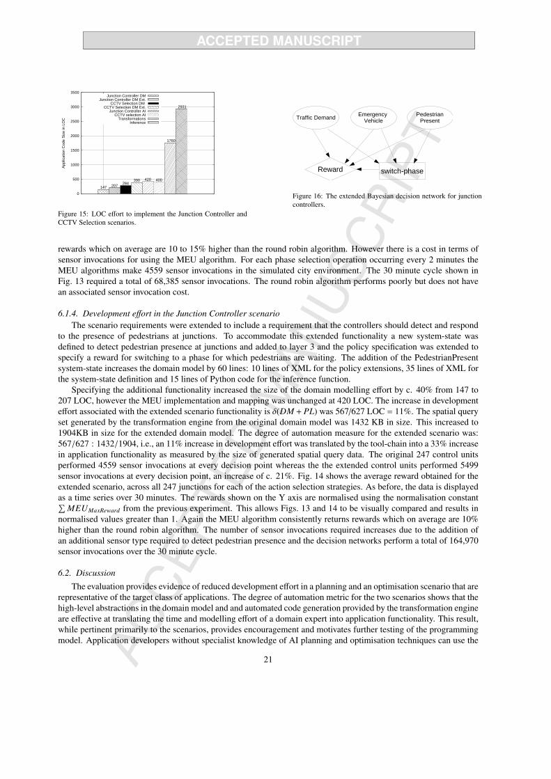
rewards which on average are 10 to 15% higher than the round robin algorithm. However there is a cost in terms ofsensor invocations for using the MEU algorithm. For each phase selection operation occurring every 2 minutes theMEU algorithms make 4559 sensor invocations in the simulated city environment. The 30 minute cycle shown inFig. 13 required a total of 68,385 sensor invocations. The round robin algorithm performs poorly but does not havean associated sensor invocation cost.

6.1.4. Development effort in the Junction Controller scenarioThe scenario requirements were extended to include a requirement that the controllers should detect and respond

to the presence of pedestrians at junctions. To accommodate this extended functionality a new system-state wasdefined to detect pedestrian presence at junctions and added to layer 3 and the policy specification was extended tospecify a reward for switching to a phase for which pedestrians are waiting. The addition of the PedestrianPresentsystem-state increases the domain model by 60 lines: 10 lines of XML for the policy extensions, 35 lines of XML forthe system-state definition and 15 lines of Python code for the inference function.

Specifying the additional functionality increased the size of the domain modelling effort by c. 40% from 147 to207 LOC, however the MEU implementation and mapping was unchanged at 420 LOC. The increase in developmenteffort associated with the extended scenario functionality is δ(DM + PL) was 567/627 LOC = 11%. The spatial queryset generated by the transformation engine from the original domain model was 1432 KB in size. This increased to1904KB in size for the extended domain model. The degree of automation measure for the extended scenario was:567/627 : 1432/1904, i.e., an 11% increase in development effort was translated by the tool-chain into a 33% increasein application functionality as measured by the size of generated spatial query data. The original 247 control unitsperformed 4559 sensor invocations at every decision point whereas the the extended control units performed 5499sensor invocations at every decision point, an increase of c. 21%. Fig. 14 shows the average reward obtained for theextended scenario, across all 247 junctions for each of the action selection strategies. As before, the data is displayedas a time series over 30 minutes. The rewards shown on the Y axis are normalised using the normalisation constant∑

MEUMaxReward from the previous experiment. This allows Figs. 13 and 14 to be visually compared and results innormalised values greater than 1. Again the MEU algorithm consistently returns rewards which on average are 10%higher than the round robin algorithm. The number of sensor invocations required increases due to the addition ofan additional sensor type required to detect pedestrian presence and the decision networks perform a total of 164,970sensor invocations over the 30 minute cycle.

6.2. Discussion

The evaluation provides evidence of reduced development effort in a planning and an optimisation scenario that arerepresentative of the target class of applications. The degree of automation metric for the two scenarios shows that thehigh-level abstractions in the domain model and and automated code generation provided by the transformation engineare effective at translating the time and modelling effort of a domain expert into application functionality. This result,while pertinent primarily to the scenarios, provides encouragement and motivates further testing of the programmingmodel. Application developers without specialist knowledge of AI planning and optimisation techniques can use the

21

tool chain to apply such techniques to their applications. For example to compare the performance of the SA algorithmto the SMOSA algorithm using the CCTV scenario domain model we can either change the complexity property fromtrue to false in the MaximalDistance system-state specification which will cause the taxonomy to automatically selectthe SA algorithm or we can override automated selection by specifying the SA algorithm be used in layer 4 ofthe domain model. Whichever technique is chosen, only one word in the domain model need be changed and thetransformation algorithms will generate a new planning model and control units with the SA algorithm embedded.

Likewise the tool chain makes it easy to extend application requirements. To extend the Junction Controllerscenario the domain expert need only define one additional system-state definition at layer 3 of the domain model andupdate the policy specification. The transformation engine will create new decision network structures as shown inFig. 16, instantiate 247 planning control units throughout the deployment environment and generate all spatial queriesnecessary for sensor fusion and state-inference.

Assuming the taxonomy can find an algorithm matching problem type and environmental conditions, it is possibleto use the tool chain to completely automate solution generation. However the CCTV Selection scenario shows thesensitivity of algorithm performance to parameter customisation, and highlights the importance of control tuningto ensure useful yet cost effective algorithm performance. The sensitivity to control tuning presents an obstacle tocompletely automating the application of planning and optimisation algorithms. Our experience of using the toolchain in the evaluation scenarios suggests that it may be more useful to use the tool chain to facilitate the rapid testingof multiple planning and optimisation algorithms over a single domain model. Layer 4 of the domain model can beused to tune parameters, while the automated transformations facilitate the rapid testing of a range of algorithms.Once algorithm selection and paramterisation have been empirically verified the generated application code can thenbe deployed.

7. Related Work

There is a growing interest in applying model-driven techniques in pervasive computing environments for purposessuch as managing the heterogeneity of devices and masking the complexity of dynamic environments. [24] proposesa model-driven approach to developing applications based on physical active objects. These are software objectsused to model sensors. The authors provide a layered reference model for designing sensor based systems and anan object oriented model containing managers for accessing and representing sensor data and application objectsto support context-aware applications. UML statecharts are used to specify the behaviour of application objects.Model transformations produce code skeletons that use the Jini middleware to bind applications to sensors. [25]presents a model-driven approach for developing context-aware applications. Environments are modelled using acombination of UML diagrams, and a PervML language developed to capture system requirements and specify theservices provided by the system. A protocol state machine specified in OCL is used to describe available services.An initial transformation algorithm parses the PervML model and generates a set of Java classes for implementingthe functionality of the specified services. A second transformation generates an OWL ontology used at runtime toidentify changing application context and facilitate adaption. These approaches focus on providing abstractions overdynamic environments rather than on providing support for AI planning and optimisation techniques. [26] proposes aplanning-based approach to supporting autonomic computing in pervasive computing environments that allows usersto specify their goals in a high-level manner and allow the planning framework to generate a plan. This approachprovides only partial support for code generation using a single planning algorithm and the modelling language usedis predicate based and non-intuitive to use.

Planning techniques have also been applied in complex service-oriented computing domains. [27] presents anapproach using planning techniques to address automatic web service composition, while [28] presents a web-servicerequest language and a planning architecture that interleaves planning and execution to allow users to express theirgoals in complex business domains. [29] proposes a service-oriented architecture that employs AI planning techniquesto orchestrate device usage in complex dynamic environments. They combine hierarchical and partial-order planningtechniques to generate abstract service workflows that are bound at runtime to actual devices present in the environ-ment. [30] presents a programming model to support the development of resource and device adaptive applications forpervasive computing environments. Application programmers use goals specified in a procedural syntax, to describewhat functionality is required. The programming model provides an extensible set of techniques that provide func-tionality to satisfy goals, and a planner responsible for evaluating techniques and binding selected techniques to goals.

22

Techniques are not planning algorithm implementations, rather they are scripts that combine and wrap code modulesand resources. Our work has a different focus in that we provide algorithms to control and optimise application state,however we maintain a similar distinction between design-time behaviour specification and runtime configuration.

Systems such as GPT and mGPT [31] from the automated planning community address real-world planningproblems and allow partially observable and dynamic planning problems to be modelled and solved theoreticallyusing the PDDL predicate-based language. Our approach is intended to complement the work of the automatedplanning community, but our focus is on generating application code instead of plans. When executed, the code isexpected to provide application functionality as specified using the domain model and policy.

8. Conclusions

This paper has presented a model-driven approach to applying AI planning and optimisation algorithms in perva-sive computing applications. Currently such knowledge is typically confined to researchers in the field and this mayact as an impediment to the deployment of such applications. The evaluation demonstrates evidence of reduced devel-opment effort in two scenarios representative of the target class of applications. Current work is focused on testing theprogramming model on a range of optimisation and planning problems and on investigating additional domain modelabstractions to allow more complex application state-space models and policies to be represented. Examples of otherabstractions that could be investigated include time, role or activity, and identity. Adding a temporal abstraction tothe domain model would allow time-dependent actions and rewards to be specified. Likewise adding role and identityabstractions would allow more traditional context-aware applications to be specified using the domain model and toaccess the planning and optimisation algorithms supported by the methodology.

The planning and optimisation functionality provided by our approach can be extended by defining mappingsfrom the planning model components to new algorithm implementations. An interesting extension would be to addreinforcement-learning algorithms to the library so that planning techniques can be used when transition systeminformation has not been specified in the domain model and must be learned from the environment. Finally, theencoding of algorithm selection criteria may be useful for the deployment of adaptive or autonomic applicationsdeployed in pervasive computing domains. Such applications could adapt to changing domain characteristics causedby mobile or non-uniform sensor and actuator coverage and dynamism, by reformulating the algorithms used forplanning and optimisation tasks in response to changes in their environment.

Acknowledgement

The work described in this paper was partly supported by Science Foundation Ireland under Investigator award02/IN1/I250 between 2003 and 2007 and grants 03/CE2/I30 and 10/CE/I1855 to Lero - The Irish Software EngineeringResearch Centre. Anthony Harrington is currently supported by an Ercim fellowship.

References

[1] J. Spall, Introduction to Stochastic Search and Optimization, Wiley InterScience, 2003.[2] M. Ghallab, D. Nau, P. Traverso, Automated Planning, Morgan Kaufmann, 2004.[3] A. Harrington, V. Cahill, Model driven engineering of planning and optimisation algorithms for pervasive computing environments, in:

PerCom 2011, March 21 - March 25, 2011, Seattle, USA, IEEE Computer Society, 2011.[4] A. Harrington, V. Cahill, Domain modelling for ubiquitous computing applications, AINA Workshop 2 (2007) 326–333.[5] M. Roman, C. Hess, R. Cerqueira, A. Ranganathan, R. H. Campbell, K. Nahrstedt, A middleware infrastructure for active spaces, IEEE

Pervasive Computing 1 (2002) 74–83.[6] D. Nicklas, M. Grossmann, T. Schwarz, Nexusscout: an advanced location-based application on a distributed, open mediation platform, in:

VLDB, VLDB Endowment, 2003, pp. 1089–1092.[7] A. Senart, R. Cunningham, M. Bouroche, N. O’Connor, V. Reynolds, V. Cahill, MoCoA: Customisable middleware for context-aware mobile

applications, in: DOA.[8] I. de Jong, Pyro – version 3.10, http://www.pyro.sourceforge.net, 2009.[9] S. K. Andersen, K. G. Olesen, F. V. Jensen, HUGIN - a shell for building Bayesian belief universes for expert systems, Morgan Kaufmann

Publishers Inc., San Francisco, CA, USA, pp. 332–337.[10] F. Jensen, Hugin api reference manual, 2007.[11] D. M. Beazley, Swig: an easy to use tool for integrating scripting languages with c and c++, in: Proceedings of the 4th conference on

USENIX Tcl/Tk Workshop, 1996 - Volume 4, USENIX Association, Berkeley, CA, USA, 1996, pp. 15–15.

23

[12] M. Bauer, C. Becker, K. Rothermel, Location models from the perspective of context-aware applications and mobile ad hoc networks,Personal Ubiquitous Comput. 6 (2002) 322–328.

[13] OpenGeoSpatialConsortium, Opengis simple features specification for sql (1999).[14] IEEE, Ieee standard for a smart transducer interface for sensors and actuators wireless communication protocols and transducer electronic

data sheet (teds) formats, IEEE Std 1451.5-2007 (????) C1 –236.[15] J. Barnett, R. Akolkar, R. Auburn, M. Bodell, D. C. Burnett, J. Carter, S. McGlashan, T. Lager, M. Helbing, R. Hosn, T. V. Raman, K. Reifen-

rath, State chart xml: State machine notation for control abstraction, W3C Working Draft, 2009.[16] L. Klein, Sensor Technologies and Data Requirements for ITS, Artech House, 2001.[17] H. F. Durrant-Whyte, Sensor models and multisensor integration, Journal of Robotics Research 7 (1988).[18] P. Maybeck, “Stochastic Models, Estimation and Control”, Academic Press.[19] K. Murphy, A survey of pomdp solution techniques - technical report university of british columbia, 2005.[20] B. Suman, P. Kumar, A survey of simulated annealing as a tool for single and multiobjective optimization, Journal of the Operational

Research Society (2006) 1143–1160.[21] F. Jensen, T. Nielsen, “Bayesian Networks and Decision Graphs”, Springer Verlag, 2007.[22] S. Russell, P. Norvig, Artificial Intelligence - A Modern Approach, Prentice Hall, 2 edition, 2003.[23] F. Webster, Traffic Signal Settings - Technical Paper No 39, Road Research Laboratory, London, UK, 1959.[24] L. Baresi, et al, Towards a model-driven approach to develop applications based on physical active objects, in: APSEC ’06.[25] E. Serral, P. Valderas, V. Pelechano, Towards the model driven development of context-aware pervasive systems, Pervasive and Mobile

Computing (2009).[26] A. Ranganathan, Autonomic pervasive computing based on planning, in: ICAC 04, IEEE Computer Society, 2004, pp. 80–87.[27] P. Traverso, M. Pistore, Automated composition of semantic web services into executable processes, in: The Semantic Web, ISWC 2004,

volume 3298, Springer Berlin / Heidelberg, 2004, pp. 380–394.[28] A. Lazovik, M. Aiello, M. Papazoglou, Planning and monitoring the execution of web service requests, Int. J. Digit. Libr. 6 (2006) 235–246.[29] J. Bidot, C. Goumopoulos, I. Calemis, Using ai planning and late binding for managing service workflows in intelligent environments, in:

PerCom 2011, March 21 - March 25, 2011, Seattle, USA, IEEE Computer Society, 2011.[30] J. M. Paluska, H. Pham, U. Saif, G. Chau, C. Terman, S. Ward, Structured decomposition of adaptive applications, Pervasive and Mobile

Computing 4 (2008) 791 – 806. PerCom 2008.[31] B. Bonet, H. Geffner, GPT: a tool for planning with uncertainty and partial information, in: IJCAI-01, Seattle, WA, pp. 82–87.

24

model-driven engineering of planning and optimisation

Documents