model checking for concurrent software architectures
TRANSCRIPT

Imperial College of Science, Technology and Medicine
University of London
Department of Computing
Model Checking
for
Concurrent Software Architectures
Dimitra Giannakopoulou
A Thesis submitted in partial fulfilment of the requirements for the degree of Doctor ofPhilosophy in the Faculty of Engineering of the University of London, and for the Diploma of theImperial College of Science, Technology and Medicine
January 1999

3
Abstract
The design of concurrent and distributed systems is generally complex, with a high possibility
that subtle errors will cause erroneous behaviour. Behaviour analysis is a powerful technique that
can help to discover behavioural anomalies at design time. The main goal of this thesis is to
develop practical and effective techniques for analysing the behaviour of concurrent and
distributed systems. To be readily usable by software developers, we emphasise that analysis
should go hand in hand with system design. Moreover, analysis techniques should be automated,
intuitive, and effective in detecting errors as well as providing guidance for error correction.
The thesis proposes the TRACTA model-checking approach for analysis of concurrent systems. A
system is modelled as a collection of labelled transition systems (LTSs), which are interacting
finite-state machines. The LTS of the system is computed from the LTSs of its subsystems, and
is checked against desired properties. In TRACTA, analysis is directed by software architecture
and, thus, it is tightly integrated with system design. In our architecture description language
Darwin, a system is described as a hierarchy of components. This hierarchy is exploited for
performing analysis in an incremental way, using Compositional Reachability Analysis (CRA).
TRACTA proposes the ALTL logic for specifying desired properties of a system. ALTL is based
on the linear temporal logic LTL, but it is specialised for concurrent systems modelled as LTSs.
To check that a system satisfies its properties, ALTL formulas are translated into Büchi
automata, following the standard automata-theoretic approach to verification. The uniqueness of
TRACTA lies in the fact that it introduces model checking naturally in CRA, as it proposes
mechanisms addressing issues that arise in this context. In addition to providing a generic
framework for property checking in CRA, the thesis identifies some classes of properties that can
be checked more efficiently. More specifically, practical checking mechanisms are provided for
safety properties as well as for a class of liveness properties, which we refer to as progress.
The thesis provides a simple and efficient way of dealing with fairness. In this context, it
introduces an action priority scheme that allows users to impose adverse scheduling conditions to
a system, during analysis. Action priority can also be used to perform a partial search on a system
that is too large to be exhaustively explored. All property-checking mechanisms discussed focus
on the detection of erroneous behaviour. To assist in error correction, counterexamples are
generated which describe a potential erroneous system execution.
TRACTA is a fully automated approach. It has been implemented in an analysis tool that has been
deployed in our environment for the development of concurrent systems. Finally, the thesis
reports on experimental results that evaluate the success of TRACTA in achieving its goals, with
realistic case studies.


5
Acknowledgements
First and foremost, I would like to thank my supervisor, Jeff Kramer. Jeff convinced me to leaveinvestment banking and join the group as a Research Associate, some four years ago. This says alot about his enthusiasm, which always gave me confidence in pursuing my ideas. Jeff’s constantguidance helped me keep in focus, and his experience and insight were invaluable for my work.
I am indebted to Jeff Magee for his practical spirit that made our discussions so stimulating. Theideas we exchanged with Jeff influenced and gave me confidence in my choices. I would alsolike to thank Shing-Chi Cheung for our exciting and fruitful collaboration.
I wish to thank Keng Ng for technical advice, but particularly for his friendship, for being suchan excellent office-mate for many years, and for singing tunes which I couldn’t help singingalong, even at the most hectic periods. Special thanks to Naranker Dulay for being “next door”.
The feedback of Naranker Dulay, Christos Karamanolis and Stephen Crane on the thesis is muchappreciated. Thanks to Ian Hodkinson for interesting discussions on temporal logic, and to IainPhillips for his comments on some of my theoretical results.
Special thanks to Morris Sloman, Jeff Kramer and Jeff Magee for arranging the computingfacilities which made this work possible, to Paul Dias and Kevin Twidle for providing technicalassistance, and to Anne O’Neill for her efficient help in administrative issues.
I am grateful to my friends and colleagues at Imperial for being such a lively and pleasant group.In particular, I would like to thank Andréa and Pomme (the best 810 and 808 that an 809 canget!), Nikos for his protective friendship, Kaveh for the “Vinceeeenzo” joke, Masoud for theGreek messages on the answering machine, Silvana for regularly reminding me that I’m terrible,Fox for the custard creams, and Manolis for a copy of “Αλέξης Ζορµπάς” on the day he thoughtof as “της Αγίας ∆ήµητρας”. Thanks also to Bashar, Celso, Damian, Douglas, Emil, Nabor, Nat,Oscar, Poomjai, Roberto, Sue, Tracy, Ulf.
I am indebted to my family Eleni, Giorgos, Liana (+�) and Manos, for more than I could everexpress.
Last but not least, I wish to thank Christos for all the support, but also for returning the cooking-favours he got while he was working on his thesis.
The work described in this thesis has been developed in the context of a general framework forthe design and construction of distributed systems, which is the result of the co-operative effortsof a number of people. The work of Shing-Chi Cheung and Jeff Kramer on CompositionalReachability Analysis set the ground for the coupling of analysis and software architecture, andtheir work on safety-property checking has been incorporated in the approach presented in thethesis. Jeff Kramer, Jeff Magee and Naranker Dulay were responsible for the design of theDarwin language. The LTSA tool was implemented by Jeff Magee, the SAA tool by Keng Ng,and the Darwin compiler by Naranker Dulay.
Financial support for this work has been provided by the EPSRC Grants GR/J87022 (TRACTAProject) and GR/M24493 (BEADS Project), by the Ioannis S. Latsis Foundation, and by theBritish Council UK/HK Joint Research Scheme project JRS96/38.


7
Στην Ελένη και το Γιώργο, τους πρώτιστους δασκάλους µου
To Eleni and Giorgos, my foremost teachers


9
Contents
1 INTRODUCTION ___________________________________________________17
1.1 Background____________________________________________________________17
1.2 Towards usable methods and tools __________________________________________20
1.3 Scope of this work ______________________________________________________21
1.4 Contributions __________________________________________________________22
1.4.1 Integrated use – Evolutionary development ____________________________________22
1.4.2 Automation – Error detection and correction ___________________________________24
1.4.3 Early benefits – Incremental gain ____________________________________________25
1.4.4 Evaluation of results ______________________________________________________25
1.5 Thesis outline __________________________________________________________25
2 MODEL CHECKING ________________________________________________27
2.1 Temporal model checking ________________________________________________28
2.1.1 Linear time______________________________________________________________30
2.1.2 Branching time __________________________________________________________32
2.2 Automata-theoretic methods_______________________________________________35
2.3 Discussion_____________________________________________________________36
2.4 Symbolic representation __________________________________________________39
2.5 On-the-fly verification ___________________________________________________41
2.6 Reduction _____________________________________________________________43
2.6.1 Partial-order reduction_____________________________________________________43
2.6.2 Compositional minimisation ________________________________________________44
2.6.3 Abstraction _____________________________________________________________50
2.7 Compositional reasoning _________________________________________________51
2.8 Discussion_____________________________________________________________52
2.9 Model-checking tools ____________________________________________________53
2.10 Summary ____________________________________________________________56
3 DESIGN & ANALYSIS ______________________________________________59
3.1 Software architecture in Darwin____________________________________________59
3.2 Modelling behaviour_____________________________________________________61
10
3.2.1 Labelled transition systems _________________________________________________61
3.2.2 Describing LTSs in FSP ___________________________________________________64
3.3 Associating behaviour with software architecture _____________________________ 66
3.3.1 The alternating-bit protocol _________________________________________________67
3.3.2 Primitive components _____________________________________________________68
3.3.3 Composite components ____________________________________________________71
3.3.4 Modelling the ABP protocol ________________________________________________73
3.3.5 Discussion ______________________________________________________________74
3.4 Compositional reachability analysis ________________________________________ 75
3.4.1 Semantic equivalences_____________________________________________________76
3.4.2 Reduction of the state space_________________________________________________77
3.4.3 CRA of the alternating-bit protocol ___________________________________________78
3.5 Related work__________________________________________________________ 82
3.6 Summary_____________________________________________________________ 84
4 MODEL CHECKING OF LTSs _______________________________________ 85
4.1 Expressing properties over actions _________________________________________ 86
4.1.1 ALTL – a linear temporal logic of actions______________________________________86
4.1.2 Introduction of alphabets into ALTL__________________________________________87
4.2 Temporal logic and finite automata ________________________________________ 89
4.2.1 Büchi automata __________________________________________________________89
4.2.2 The role of alphabets ______________________________________________________90
4.2.3 Büchi processes __________________________________________________________92
4.3 Program verification ____________________________________________________ 95
4.3.1 Procedure_______________________________________________________________96
4.3.2 Example________________________________________________________________98
4.4 Safety and liveness _____________________________________________________ 99
4.5 Checking properties in the context of CRA _________________________________ 101
4.5.1 Observational equivalence and model checking ________________________________101
4.5.2 Reasoning about hidden actions ____________________________________________104
4.6 Optimisation of the RD algorithm_________________________________________ 107
4.7 Discussion___________________________________________________________ 109
4.8 Summary____________________________________________________________ 110
5 ANALYSIS STRATEGIES: SAFETY ___________________________________113
5.1 Safety properties ______________________________________________________ 113
5.1.1 Verification ____________________________________________________________115
11
5.1.2 Correctness ____________________________________________________________117
5.1.3 Non-deterministic safety properties__________________________________________119
5.2 Alternating-bit protocol revisited __________________________________________120
5.3 Safety properties as ALTL formulas _______________________________________125
5.4 Expressiveness and efficiency ____________________________________________127
5.5 Summary_____________________________________________________________129
6 ANALYSIS STRATEGIES: LIVENESS _________________________________131
6.1 Fairness considered_____________________________________________________131
6.2 Adding fairness constraints to process behaviour______________________________134
6.3 Fair choice ___________________________________________________________136
6.3.1 Checking liveness under fair choice _________________________________________136
6.3.2 Action priority __________________________________________________________138
6.4 Progress properties _____________________________________________________141
6.5 Example: readers-writers ________________________________________________144
6.6 Discussion____________________________________________________________147
6.7 Deterministic Büchi processes ____________________________________________148
6.8 General methodology ___________________________________________________150
6.9 Summary_____________________________________________________________151
7 IMPLEMENTATION & EVALUATION__________________________________153
7.1 Environment __________________________________________________________153
7.2 Tool implementation____________________________________________________155
7.2.1 System construction______________________________________________________155
7.2.2 System analysis _________________________________________________________157
7.2.3 Interface and additional features ____________________________________________158
7.3 Case study: a reliable multicast transport protocol_____________________________160
7.3.1 The protocol____________________________________________________________160
7.3.2 Structure of the RMTP ___________________________________________________161
7.3.3 Modelling component behaviour for the RMTP ________________________________163
7.3.4 Property specification ____________________________________________________167
7.3.5 Checking the RMTP protocol ______________________________________________169
7.4 Evaluation and discussion________________________________________________175
7.4.1 Analysis and software architecture __________________________________________175
7.4.2 The cost of minimisation __________________________________________________177
7.5 Summary_____________________________________________________________178

12
8 CONCLUSIONS __________________________________________________181
8.1 Contributions_________________________________________________________ 181
8.1.1 Analysis and software architecture __________________________________________181
8.1.2 Model checking _________________________________________________________182
8.1.3 Tools _________________________________________________________________183
8.2 Critical evaluation_____________________________________________________ 183
8.2.1 Integrated use – Evolutionary development ___________________________________183
8.2.2 Automation – Error detection and correction __________________________________184
8.2.3 Early benefits – Incremental gain ___________________________________________186
8.3 Future work__________________________________________________________ 186
8.3.1 Improvement of current mechanisms ________________________________________187
8.3.2 Focused application and increased flexibility __________________________________187
8.4 Closing remark _______________________________________________________ 188
REFERENCES _____________________________________________________189
APPENDICES ______________________________________________________201
A Labelled Transition Systems ______________________________________________ 203
B FSP Quick Reference____________________________________________________ 209
C FSP Semantics _________________________________________________________ 213
D Theorems and Proofs ____________________________________________________ 217

13
List of Figures
Figure 1.1: Tool support for system design and analysis _______________________________23
Figure 2.1: Approaches to model checking _________________________________________27
Figure 2.2: Approaches to controlling state explosion _________________________________28
Figure 2.3: Unwinding a Kripke structure into an infinite finitary tree ____________________34
Figure 2.4: Ordered binary decision tree and OBDD for (a∧b)∨(c∧d) with variable ordering
a<b<c<d ________________________________________________________________39
Figure 2.5: InterfaceI increases the size of subsystemP_______________________________48
Figure 3.1: Common structural view with service and behavioural views__________________60
Figure 3.2: LTS models of a lamp and a student, and LTS of their joint behaviour __________62
Figure 3.3: LTSs that demonstrate relabelling and hiding ______________________________64
Figure 3.4: Primitive component for a simple counter in Darwin ________________________68
Figure 3.5: Behavioural description of an infinite and a bounded counter__________________69
Figure 3.6: Primitive component for a “proper” transmitter in Darwin ____________________70
Figure 3.7: Darwin description of the protocol transmitter _____________________________72
Figure 3.8: Structure of the ABP component ________________________________________73
Figure 3.9: Compositional hierarchy for the ABP protocol _____________________________77
Figure 3.10: LTS for ABP with infinite retransmissions and infinite channels ______________81
Figure 4.1: Temporal interpretation defined by an infinite sequence of actions _____________87
Figure 4.2: Interpretation defined by (enter1 exit1 enter2 exit2)ω__________________________88
Figure 4.3: Büchi automaton and Büchi process for formula□(request⇒ ◊ granted) ________89
Figure 4.4: A Büchi automaton representing formulaf = □(a ⇒ ◊b)______________________91
Figure 4.5: A Büchi process modelling fair choice between two alternatives _______________92
Figure 4.6: Transformation of a Büchi automaton into a Büchi process ___________________93

14
Figure 4.7: Minimised ABP protocol, and Büchi process for◊(accept.1 ∧ □¬ deliver.1) ____ 99
Figure 4.8: Composite LTS of ABP with property L1 ________________________________ 99
Figure 4.9: Disappearance ofτ-cycles during minimisation___________________________ 101
Figure 4.10: An algorithm that records divergence _________________________________ 102
Figure 4.11: LTSs with divergence recorded ______________________________________ 102
Figure 4.12: Structure of component TRANS_CHNL of the ABP protocol ______________ 103
Figure 4.13: After applying the RD algorithm, minimisation preserves violations _________ 107
Figure 4.14: Behaviour of stateπ (represented as –1) during composition _______________ 108
Figure 4.15: Optimised algorithm for recording divergence___________________________ 108
Figure 5.1: Mutual exclusion property ___________________________________________ 114
Figure 5.2: Image process for mutual exclusion property_____________________________ 115
Figure 5.3: Checking mutual exclusion __________________________________________ 116
Figure 5.4: Transformation from non-deterministic to deterministic property LTS_________ 119
Figure 5.5: Property RIGHT_IGNORE of the ABP _________________________________ 120
Figure 5.6: Compositional hierarchy for the ABP protocol ___________________________ 122
Figure 5.7: Büchi process for property WRONG_IGNORE __________________________ 126
Figure 5.8: Relative expressiveness of ALTL, safety-property LTSs, and Büchi
automata/processes ______________________________________________________ 128
Figure 6.1: A simple client-server system_________________________________________ 132
Figure 6.2: Using Büchi processes to impose fairness constraints ______________________ 135
Figure 6.3: System consisting of a server and two clients, one of which may crash ________ 135
Figure 6.4: Using action priority to obtain various types of channels ___________________ 139
Figure 6.5: Action priority is not compositional____________________________________ 140
Figure 6.6: LTS for RDRS_WRTRS ____________________________________________ 145
Figure 6.7: LTS for RW_STRESS ______________________________________________ 146
Figure 6.8: Büchi process used for checking progress property WRITER________________ 147
Figure 6.9: Classes of properties supported by TRACTA______________________________ 150

15
Figure 7.1: Tool support for design and analysis of distributed systems __________________154
Figure 7.2: The Software Architect’s Assistant (SAA) _______________________________155
Figure 7.3: Interface of the LTSA tool ____________________________________________158
Figure 7.4: Animation of the coin tossing example __________________________________160
Figure 7.5: A multicast tree of receivers___________________________________________161
Figure 7.6: Structure of an ordinary receiver in the RMTP ____________________________162
Figure 7.7: Compositional hierarchy for the RMTP__________________________________163
Figure 7.8: Safety property for the RMTP _________________________________________168
Figure 7.9: Liveness properties for the RMTP ______________________________________169
Figure 7.10: AnimatingDES_REC_Bfor deadlock scenario___________________________171
Figure 7.11: Abstracted LTS obtained for the RMTP after verification___________________173

16

17
Introduction 11.1 BACKGROUND 17
1.2 TOWARDS USABLE METHODS AND TOOLS 20
1.3 SCOPE AND CONTRIBUTION OF THIS WORK 21
1.4 THESIS OUTLINE 25
1.1 Background
With the inevitable increase in complexity of both hardware and software systems, the likelihood
of subtle errors is high. Such errors may have catastrophic consequences in terms of money,
time, or even human life. In general, the earlier an error is discovered, the cheaper it is to fix. In
the industry, there is therefore a growing demand for methodologies that can increase confidence
in correct system design and construction. Such methodologies will result in improved quality, as
well as in a reduction to the total development cost of a system. Additionally, purely on the
theoretical side, there is a need to provide a sound mathematical basis for the design of computer
systems, which can offer practising engineers the confidence of combining their experience with
a solid methodological framework.
The traditional engineering approach to construction of complex systems is to build models.
Models can be studied and modified until confidence is obtained in their correctness. The
advantage is that models are simpler, represent the particular aspects of interest of the system,
and their development cost is negligible when compared to the cost of building the system itself.
Formal verification advocates a similar approach to the construction of computing systems.
Formal verification means creating a mathematical model of a system, using a language to
specify desired properties of the system in a concise and unambiguous way, and using a method
of proof to verify that the specified properties are satisfied by the model. When the method of
proof is carried out substantially by machine, we speak ofautomatic verification. Two well-
established methods to verification are theorem proving and model checking.
In theorem proving, both the system and its desired properties are expressed as formulas in some
mathematical logic. The system satisfies a property if a proof can be constructed in that logic for

CHAPTER 1 INTRODUCTION
18
the property, from the axioms of the system. This is a powerful approach, which can deal directly
with infinite state spaces. It relies on techniques such as structural induction to prove over
infinite domains. However, the approach involves user interaction in selecting the inference
procedures to be applied. It often involves the generation and proof of a large number of lemmas,
which are likely to discourage even mathematically oriented designers. The following is taken
from the Web page of PVS (http://pvs.csl.sri.com) [Owre, et al. 96], one of the most widely used
theorem provers: “PVS is a large and complex system and it takes a long while to learn to use it
effectively. You should be prepared to invest six months to become a moderately skilled user
(less if you already know other verification systems, more if you need to learn logic or unlearn
Z)”. Unfortunately, approaches that involve unfamiliar notations and require expertise before any
benefits can be obtained from their use are unlikely to be appealing to the average software
engineer.
In model checking, a finite model of a system is built and checked against a set of desired
properties. Model checking is more limited in scope than theorem proving, but is fast and fully
automated. The system model is in essence a finite-state machine, which is intuitive to the
average engineer. The system may be expressed directly in terms of state machines.
Alternatively, a subset of some higher-level language may be used, which permits more concise
specifications, while restricting the developer to finite-state models that can be handled by the
model-checking approach. For example, there exist tools that support the CCS and CSP process
algebras [Cleaveland, et al. 93b, Roscoe 94], and standard specification languages such as
LOTOS or SDL [Fernandez, et al. 96].
In model checking, desired properties are usually expressed either in some temporal logic [Pnueli
81] or in terms of automata [Vardi and Wolper 86]. An exhaustive search of the state space is
performed in order to check that the system is a model of its specifications – hence the term
“model checking”. This search is guaranteed to terminate, since the model is finite. When both
the system and its specifications are modelled as finite-state machines, the system can also be
compared to the specification to determine whether its behaviourconforms to that of the
specification. Various notions of conformance have been used, such as refinement orderings
[Cleaveland, et al. 93b, Roscoe 94] or bisimulation relations [Cleaveland, et al. 93b, Fernandez,
et al. 96].
Unfortunately, modelling complex systems as finite-state machines has an inherent disadvantage,
commonly known asstate explosion. This problem describes the exponential relation of the
number of states in the model of a system, to the number of components of which the state is
made. As a result, model checking cannot handle efficiently systems that are made up of a large

CHAPTER 1 INTRODUCTION
19
number of (even small) state machines, nor with systems that manipulate data. In general, model
checking is only applicable to systems whose states have short and easily manipulated
descriptions [Wolper 95]. Typically, systems in this category concentrate on control, for instance
hardware, concurrent protocols, process control systems, and more generally what are referred to
as reactive systems [Manna and Pnueli 92]. These are systems whose role is more readily
described by their possible interaction sequences with their environment than by the
transformation they apply to complex data.
The main technical challenge in the area of model checking is to devise methods and data
structures that handle large state spaces. With the advent of new model-checking approaches, the
size of systems that can be handled has increased considerably. For example, [McMillan 93] used
ordered binary decision diagrams [Bryant 86] to represent state-transition systems efficiently.
The approach, also known assymbolic model checking, is particularly effective for systems with
regular structure such as hardware circuits [Burch, et al. 94, Clarke, et al. 93b]. Another approach
to state explosion is based onreduction, which consists of reducing the size of the state space
that needs to be explored.Partial order reductionis such a technique; it avoids the generation of
all paths formed by interleaving the same set of transitions [Godefroid and Wolper 91,
Holzmann, et al. 92].Reduction by compositional minimisationis another; it bases reduction on
intermediate simplification of subsystems [Cheung and Kramer 96b, Yeh and Young 91].
Admittedly, no single approach to formal verification is able to serve all purposes. For this
reason, verification tools are moving towards becoming tool-sets that support various approaches
to model checking [Fernandez, et al. 96, Holzmann 97]. Some of the existing theorem provers are
also moving towards the integration of model checking with theorem proving [Bjørner, et al. 96,
Owre, et al. 96].
Model checking and theorem proving have been tried in a number of industrial case studies, and
errors have been discovered in protocols and designs [Clarke and Wing 96a]. Thanks to advances
from research in this area, the industry is now gradually introducing such techniques in the
system development process. Model checking is practical, fast and fully automated but inherently
vulnerable to state explosion. Theorem proving is powerful and flexible, but not as intuitive to
apply. We believe that due to its intricacy, theorem proving will be established as a task for
expert users, and for safety-critical systems that cannot be handled by model checking. Model
checking, on the other hand, will become established as a widely accessible method, although of
more limited scope. As this thesis is particularly concerned with the issues of usability and
accessibility of formal verification methods, it only deals with model checking.

CHAPTER 1 INTRODUCTION
20
1.2 Towards usable methods and tools
According to [Clarke and Wing 96a], experience has produced a number of criteria that play a
significant role in making methods and tools attractive to practising engineers. It is important for
such criteria to be taken into consideration if usability is the main goal in developing methods
and tools. In this section, we discuss a set of such criteria that we consider realistic, and which
have motivated our approach to formal verification.
1. Early benefits.In order to encourage practising engineers to use them, methods should
require a minimal effort before engineers realise the benefits from their use. Notations should
be clear and intuitive to the average user. Tools should have friendly user-interfaces that
make them easy to use, and their output should be easy to understand.
2. Incremental gain.Developers should obtain increasing benefit as they put more effort into
learning methods and tools in depth. Ideally, tools should support various modes for users
with various abilities. They should be appealing to the beginner, but should also provide
more sophisticated analysis capabilities for experienced and more demanding users.
3. Integrated use.Analysis should not be an isolated phase in the software development
process. Rather, methods and tools for design, analysis and construction should be well
integrated, and support similar approaches to system development.
4. Evolutionary development.Methods and tools should support incremental system
development as well as component reusability.
5. Automation. The higher the degree of automation of a tool, the higher its usability.
Approaches that require user interaction expect the user to have a good knowledge of their
underlying methodology, and are, as a result, mainly addressed to developers with expertise
in the specific approach. Automated tools are more widely accessible, and more readily
usable.
6. Error detection and correction.It is not enough for a method to be able to certify
correctness. Rather, it is essential for it to concentrate on error detection and correction. For
correction, methods should support the generation of counterexamples. Counterexamples are
an invaluable guide to debugging because they provide an example execution of the system
that leads to the error detected.

CHAPTER 1 INTRODUCTION
21
7. Focused application.As mentioned, no single method can serve all purposes. Therefore, it is
desirable that methods concentrate on dealing efficiently with at least one aspect of a system,
or on addressing at least one range of applications. Particular emphasis should therefore be
placed on identifying and stating explicitly the strengths and weaknesses of the methods
developed. It is essential to provide potential users with clear criteria for selecting the
method and tool that is most appropriate to their needs.
8. Flexibility. In order to be able to handle complex systems of different kinds, and various
aspects of these systems, it is desirable for tools to accommodate multiple approaches to
formal verification, as well as to support a variety of input notations. It is, however, difficult
to achieve an integration of methods that is meaningful, without being over-complicated.
1.3 Scope of this work
Concurrent and distributed systems are no longer rare, but are widely used in applications from
television sets to train signalling and workflow systems. The order in which events occur in the
execution of such systems is unpredictable and only restricted by synchronisation of individual
processes. As a result, the design of distributed systems is generally complex, with a high
probability that subtle errors will cause erroneous behaviour. Without the assistance of automated
tools, it is particularly difficult for the developers of such systems to be confident about the
correctness of their designs.
Our main goal is the development of practical and effective techniques with tool support for
analysing the behaviour of concurrent and distributed systems. More specifically, we focus on
model-checking methods and tools that can be easily introduced into the system development
process, and are accessible to and usable by practising engineers.
The work presented in this thesis builds on previous experience with design and analysis of
distributed systems, within our research team. In our environment, the design of such systems is
based on the description of their software architecture in Darwin [Magee, et al. 95]. Darwin
describes a system as a hierarchy of components that implement services, and additionally
specifies component interactions. It has been extensively used for specifying the structure of
distributed systems and subsequently directing their construction. The Software Architect’s
Assistant [Ng, et al. 96] is a visual environment for the design and development of distributed
software using Darwin architectural descriptions.

CHAPTER 1 INTRODUCTION
22
Concurrent and distributed systems are examples of reactive systems, whose intricacy resides in
the communication between their components. Such systems can be modelled in terms of
Labelled Transition Systems (LTSs). An LTS is an interacting finite-state machine that describes
the behaviour of a process in terms of the communication events in which it may engage.
Our experience with analysis was related to the use of compositional reachability analysis (CRA)
to compute system behaviour [Cheung 94c]. According to this, a distributed system is
decomposed in a hierarchy of subsystems, and the behaviour of each primitive subsystem is
modelled as an LTS. The LTS of the system is then obtained stepwise, by composing and
simplifying the LTSs of its subsystems. As a compositional minimisation approach, CRA may
significantly reduce state explosion. However, it is susceptible to intermediate state explosion, a
problem that occurs when components of a system explode faster than the system itself. When
constrained by activities of their context, these components usually have a much smaller state
space. A way of addressing this problem is to use specific processes, namedinterfaces, to
constrain the behaviour of subsystems according to their context. [Cheung 94c] proposed
techniques for generating interfaces automatically.
1.4 Contributions
We have developed the TRACTA model-checking approach, which places particular emphasis on
better method and tool usability. The following is an overview of the characteristics and
contributions of TRACTA, based on the usability criteria presented in Section 1.2.
1.4.1 Integrated use – Evolutionary development
A major contribution of our work is that we have integrated analysis in a general environment for
the support of distributed systems development. As described below, our methods and tools work
in conjunction with each other, and offer a consistent environment for design, analysis, and
construction of distributed systems.
TRACTA achieves a tight integration of analysis with design in our environment, by using the
hierarchical structure of a system’s software architecture, to direct CRA. The developer can thus
avoid redundant effort of re-defining system structure for every activity of software development.
TRACTA defines mappings between features of the Darwin language and operators of the LTS
model. In this way, system structure described in Darwin is automatically translated into a form
that can be used directly by our analysis tools.
CHAPTER 1 INTRODUCTION
23
Darwin supports hierarchical system design thus allowing developers to build their systems
incrementally. Our analysis techniques should similarly support incremental generation and
analysis of system behaviour. Indeed, CRA enforces an incremental approach to analysis, since
the behaviour of sub-components of a system can be analysed locally, during intermediate stages
of analysis.
PRIMITIVE COMPONENT
BEHAVIOUR + PROPERTIESREQUIREMENTS,
CHANGES
SYSTEM
ARCHITECTURE
SYSTEM
INSTANCE
SYSTEM STRUCTURE
SAA LTSA
DARWINCOMPILER
ANALYSIS
RESULTS
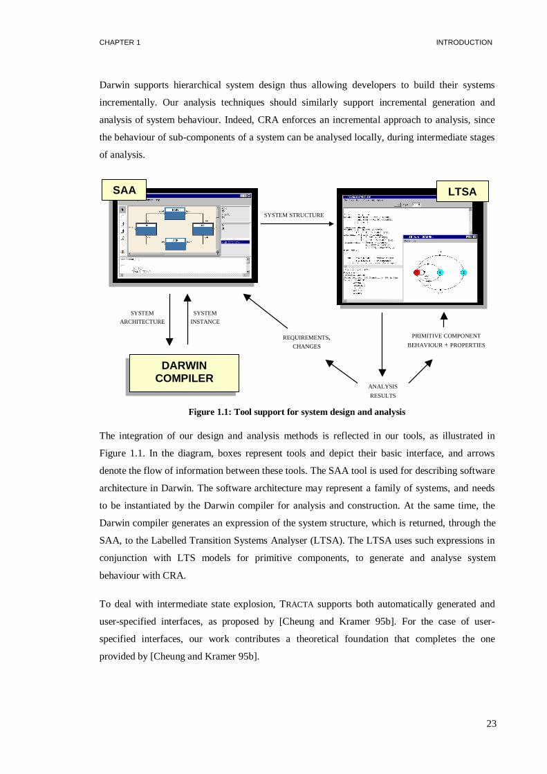
Figure 1.1: Tool support for system design and analysis
The integration of our design and analysis methods is reflected in our tools, as illustrated in
Figure 1.1. In the diagram, boxes represent tools and depict their basic interface, and arrows
denote the flow of information between these tools. The SAA tool is used for describing software
architecture in Darwin. The software architecture may represent a family of systems, and needs
to be instantiated by the Darwin compiler for analysis and construction. At the same time, the
Darwin compiler generates an expression of the system structure, which is returned, through the
SAA, to the Labelled Transition Systems Analyser (LTSA). The LTSA uses such expressions in
conjunction with LTS models for primitive components, to generate and analyse system
behaviour with CRA.
To deal with intermediate state explosion, TRACTA supports both automatically generated and
user-specified interfaces, as proposed by [Cheung and Kramer 95b]. For the case of user-
specified interfaces, our work contributes a theoretical foundation that completes the one
provided by [Cheung and Kramer 95b].

CHAPTER 1 INTRODUCTION
24
1.4.2 Automation – Error detection and correction
As a model-checking approach, TRACTA is fully automated. The LTSA tool (Figure 1.1), which
currently supports TRACTA, has been based on experience gained from the extensive use of a tool
developed as part of this work [Giannakopoulou, et al. 97]. The LTSA has the advantage of being
implemented in Java, and is therefore cross-platform. It also provides an intuitive user-interface
that facilitates the use of our methods.
Our approach contributes a variety of model-checking mechanisms, as described below.
• TRACTA proposes the logic ALTL (Action Linear Temporal Logic) for specifying desired
properties of a system. ALTL is based on the linear temporal logic LTL [Gribomont and
Wolper 89], but it is specialised for reasoning about concurrent systems modelled as LTSs.
• TRACTA adopts the automata-theoretic approach to model checking [Gribomont and
Wolper 89, Vardi and Wolper 86]. It can check properties expressed directly as Büchi
automata, or as ALTL formulas that are translated into Büchi automata for verification. The
uniqueness of TRACTA lies in the fact that it addresses issues related to model checking in the
context of CRA. It provides efficient model-checking mechanisms that introduce model
checking naturally in our framework, where software architecture is used to direct CRA.
• In addition to generic mechanisms for checking properties expressed as Büchi automata,
TRACTA provides practical analysis strategies for certain classes of properties. Specifically, it
proposes mechanisms for checking safety properties, liveness properties expressed as
deterministic Büchi automata, and a class of liveness properties to which we refer as
progress. All these techniques are integrated in a methodology described in this thesis.
• TRACTA proposes a simple and efficient way of dealing with fairness. In this context, it
introduces an action priority scheme that allows users to impose adverse scheduling
conditions to a system, during analysis. Action priority can also be used to perform a partial
search on a system that is too large to be exhaustively explored by our tools.
Every checking mechanism in TRACTA concentrates on locating system behaviour that violates
desired properties. When errors are detected, TRACTA returns counterexamples, which describe a
potential erroneous system execution. The LTSA tool supports the facility of interactive
simulation, which allows the user to examine the effects of any scenario on individual
components of a system. In conjunction with counterexamples, this facility provides invaluable
assistance in the task of diagnosing and correcting errors in the model of a system.
CHAPTER 1 INTRODUCTION
25
1.4.3 Early benefits – Incremental gain
In the LTSA tool, behaviour is specified in terms of a notation called FSP (Finite State
Processes), with LTS semantics. FSP has been developed by our research team [Magee, et al.
97]. The notation is easy to learn and use, and facilitates the translation from Darwin. The LTSA
provides the possibility of checking FSP specifications by graphically displaying the
corresponding LTSs. Initially, our plans involved a graphical input to our analysis tools, but we
soon realised that this becomes cumbersome for systems that contain more than a few states.
As discussed, TRACTA supports several model-checking techniques that address users of
different levels of expertise. For simple experimentation with the model of a system, interactive
simulation can be applied. Inexperienced users can also perform default deadlock and progress
checks, and can use templates to specify properties of a system. Users that invest time in learning
the method and tool are given the opportunity of performing more elaborate analysis. They can
express properties in any form supported by the approach, include fairness considerations to
analysis, and apply action priority. They can additionally experiment with alternative checking
mechanisms.
1.4.4 Evaluation of results
The approach advocated in the thesis is evaluated with a number of case studies. These case
studies concentrate on estimating how successful TRACTA has been in achieving its main goals.
More specifically, they demonstrate how the phases of design and analysis are integrated with the
use of software architecture. Furthermore, they evaluate the effectiveness of the various model-
checking mechanisms proposed by our approach. Finally, they compare TRACTA to similar
approaches with respect to the way they handle state explosion.
1.5 Thesis outline
Chapter 2 presents the factors that inhibit the introduction of model checking in the software
development process, especially for industrial applications. The main advances made for
overcoming these problems are analysed. Several successful model-checking tools and the
approaches that they implement are also discussed.
Chapter 3 describes the way in which analysis methods have been integrated in our environment
for the development of concurrent and distributed systems. The basic features of the Darwin
architecture description language are presented, in conjunction with their corresponding features

CHAPTER 1 INTRODUCTION
26
in the FSP language. We then introduce CRA, problems related to it, as well as the way in which
software architecture is used to guide CRA.
Chapter 4 motivates and describes the use of ALTL for expressing properties of LTSs. A
generic mechanism is then provided for checking that a system satisfies properties expressed as
ALTL formulas or Büchi automata. This mechanism is then adjusted to cope with issues that
arise when CRA is used to construct the LTS of a system.
Chapter 5 concentrates on the issue of safety-property checking. Safety properties can be
specified with a less expressive model than Büchi automata. This model is amenable to an
efficient checking mechanism, described in this chapter. A similar technique is presented, for
checking correctness of user-specified interfaces in the context of CRA.
Chapter 6 discusses the notion of fairness, and relates it to liveness property checking. It
proposes efficient strategies for checking liveness properties expressed as deterministic Büchi
automata, and for checking a class of liveness properties termed progress. Such checks are
performed under specific fairness assumptions about the system execution, which can be refined
with the use of an action priority scheme. The chapter concludes with a methodology that users
are advised to follow for analysing their systems. The methodology encourages the gradual
transition from efficient and inexpensive checks that may not detect all possible errors in the
system, to tests that are more expensive but also more thorough.
Chapter 7 describes the construction and use of our analysis tool, as well as the way in which it
interacts with our other tools for the development of concurrent and distributed systems. The
non-trivial case study of a Reliable Multicast Transport Protocol is used to evaluate the
applicability, performance and efficiency of our approach, and to compare it with similar
approaches.
Chapter 8 summarises and evaluates the contribution of TRACTA to model checking, discusses
open issues and explores directions for future work.
Appendix A is a formal presentation of the LTS model.Appendix B is a quick reference for the
FSP language.Appendix C provides the semantics of the FSP language. Finally,Appendix D
presents the proofs of some theorems and lemmas used in the main body of the thesis.

27
Model Checking 22.1 TEMPORAL MODEL CHECKING 28
2.2 AUTOMATA-THEORETIC METHODS 35
2.3 DISCUSSION 36
2.4 SYMBOLIC REPRESENTATION 39
2.5 ON-THE-FLY VERIFICATION 41
2.6 REDUCTION 43
2.7 COMPOSITIONAL REASONING 51
2.8 DISCUSSION 52
2.9 MODEL-CHECKING TOOLS 53
2.10 SUMMARY 56
As mentioned in the introduction, model checking relies on creating a finite model of a system
and checking that model against its desired properties. The system model is in essence a finite-
state machine. Given that the model is finite, it is possible to perform an exhaustive state-space
exploration for checking that the model satisfies its specifications. System specifications are
typically expressed in some temporal logic or as automata, giving rise to two general approaches
to model checking that are used in practice today [Clarke and Wing 96a]: temporal model
checking and automata-theoretic model checking, respectively (Figure 2.1).
MODEL CHECKING
TEMPORAL LOGIC AUTOMATA THEORETIC
Figure 2.1: Approaches to model checking
Any model-checking technique suffers from an inherent limitation commonly known asstate
explosion. This describes the exponential relation of the number of states in the model of a
system, to the number of components that make up the system states. The main technical
challenge in the area of model checking is to devise methods and data structures that handle large
state spaces. A number of methods have been proposed for avoiding state explosion. These
methods fall roughly into four main categories (Figure 2.2).

CHAPTER 2 MODEL CHECKING
28
Symbolic representationtechniques try to avoid state explosion by representing state transition
systems implicitly, using binary decision diagrams. Since the model of the system is represented
symbolically, there is no need to construct it as an explicit data structure.On-the-fly model
checkingconsists of verifying the system during its generation. It simulates all possible transition
sequences that the system is able to perform in a depth-first traversal of the system graph,
without storing its transitions; the search stops after any error has been located, which is often
well before the whole state space has been explored.Reduction methods are based on
transforming the verification problem into an equivalent problem in a smaller state space.
Finally, compositional reasoningis based on identifying local properties of subsystems that
guarantee desired properties for the global system. In this way, the global state graph does not
need to be generated, since properties of subsystems are checked instead.
This chapter discusses model checking in terms of the above categories. Temporal and automata-
theoretic model checking are described at first. The main approaches to state explosion are then
discussed. Finally, an overview is made of existing model-checking tools.
STATE EXPLOSION CONTROL
SYMBOLIC
REPRESENTATION
ON-THE-FLY
REDUCTION
PARTIAL ORDER COMPOSITIONAL
MINIMISATION
ABSTRACTION
COMPOSITIONAL
REASONING
Figure 2.2: Approaches to controlling state explosion
2.1 Temporal model checking
Temporal model checking is a technique developed independently by [Clarke, et al. 83], and
[Queille and Sifakis 82]. In this approach, desired properties of a system are expressed in terms
of a propositional temporal logic. Temporal logics have proven to be useful for specifying
concurrent systems, because they can describe the ordering of events in time without introducing
time explicitly [Clarke, et al. 93a]. As it is not necessary to use past operators for program

CHAPTER 2 MODEL CHECKING
29
verification, we restrict our discussion to tense operators that involve the present and future. The
terminology used follows that of [Gribomont and Wolper 89].
A temporal frameis a pair (S, R) whereS is a set of time instants, andR is a relation onS that
relates each instant with itsimmediatesuccessor(s). The reflexive transitive closure ofR, denoted
as≤, represents temporal order:s ≤ t denotes that instants occurs beforet, or s andt correspond
to the same time instant. The nature of theR relation gives rise to two different models of time
and logics:branching-timeandlinear-timetemporal logic.
Given a setP of atomic propositions, atemporal interpretationI is a triple (S, R, I), where (S, R)
is a temporal frame, andI is an interpretation functionthat defines a mapping fromS × P to
{ true, false}. In other words, I assigns a truth-valueI(s, p) to each time instant inS, and
proposition inP. A temporal logic defines semantic rules for the operators of that logic. Given an
interpretation (S, R, I), these rules assign a truth-value to each pair consisting of a time instant in
S, and a formula of the logic.
Desired properties of a program can be expressed as formulas in some temporal logic. As
described in the following, the state-transition system that represents a program can be thought of
as a (set of) temporal interpretation(s) in that logic. Temporal model checking then consists of
checking if the properties of the program are true in the interpretation(s) defined by the program.
When violations of properties are detected, the model-checking algorithms return
counterexamples, i.e. examples of system executions that exhibit erroneous behaviour. As such,
counterexamples provide invaluable guidance in debugging the design of a system.
Kripke structures
In this chapter, we assume, for simplicity, that systems are modelled as finite Kripke structures
[Hughes and Cresswell 68]. A finite Kripke structure is a 5-tuple (S, q, P, L, R), whereS is a
finite set of states,q ∈ S is the initial state,P is a finite set of atomic propositions,L:S → 2P is a
function that labels each state with the set of atomic propositions that hold at that state, and
R⊆S×S is a transition relation. Assume that a system is associated with a vector of state variables
(u0, u1, …, un). Then each states = (x0, x1, …, xn) in its Kripke model represents a specific
assignment of values (ui=xi) to the system state variables. Atomic propositions will usually be of
type (ui equalsa), and will be true in all states (x0, x1, …, xn) for whichxi=a.
Let M = (S, q, P, L, R) be the Kripke model of a program. We assume that in general, relationR
is total, which means that for every states ∈ S, ∃ s´ such that (s, s ) ∈ R. A path p in M is an
CHAPTER 2 MODEL CHECKING
30
infinite sequence of states (s0, s1, s2, …), such that∀i ≥ 0, (si , si+1) ∈R. We say thatp=(s0, s1, s2,
…) is rootedat states0.
2.1.1 Linear time
In linear temporal logic (LTL), time is a linearly ordered set, usually measured with natural
numbers. In a linear frame (S, R), R is a functional relation that assigns to each time instant
exactly one immediate successor. The temporal order≤ in LTL is a total order, i.e. for any two
time instantss, t ∈ S, eithers ≤ t or t ≤ s. It is customary to give the semantics of this logic in
terms of the frame (N, Succ), whereN is the set of natural numbers andSucc(Succ(n) = n+1) is
the standard successor function on that set. In this semantics, an interpretation can also be seen as
an infinite sequence of assignments of truth-values to the atomic propositions [Gribomont and
Wolper 89].
Syntax
The language of linear-time temporal logic (LTL) is that of propositional calculus augmented
with the following fourtemporal operators:
○ – unary operator, read “at the next time”; U – binary operator, read “until”.
□ – unary operator, read “always”; ◊ – unary operator, read “eventually”;
All syntactic rules of propositional logic are also rules of LTL. Moreover, iff andg are formulas
of LTL, then so are○f, □f, ◊f, f U g.
Semantics
A linear-time temporal interpretationI = (N, Succ, I) assigns a truth-value to any formula of LTL
at any time instants ∈ N in the following way:
• I(s, f) = I(s, f), ∀ f∈P, whereP is the set of atoms
Logical operators:
• I(s, f∧g) = I(s, f) ∧ I(s, g) • I(s, ¬f) = ¬I(s, f)
The semantics of the remaining logical operators can be defined in terms of the above.
Temporal operators:
• I(s, ○f) = I(s+1, f)

CHAPTER 2 MODEL CHECKING
31
• I(s, f U g) = true iff ∃ j∈N . I(s+j, g) = true and∀ 0 ≤ i < j, I(s+i, f) = true
• I(s, □f)= true iff I(s+i, f) = true, ∀ i ≥ 0
• I(s, ◊f) = true iff ∃ j∈N . I(s+j, f) = true
The operatorU that we have defined, is often referred to as “strong until” as opposed to “weak
until”, which we denote asUW. “Weak until” has similar semantics to “strong until”, with the
addition that (f UW g) is also true whenf is always true. In fact, it may be expressed in terms of
strong until as follows: (f UW g) = (f U g) ∨ □f. Note that the semantics of operators◊ and□ has
been explicitly described here in order to clarify their use to the reader. However, these operators
are simply abbreviations for the following formulas:◊f = (trueU f), and□f = ¬◊¬f.
Verification
Let M = (S, q, P, L, R) be the Kripke model of a program. Each pathp = (s0, s1, s2, …) in M
defines a temporal interpretationI as an infinite sequence of assignments of truth values to
atomic propositions inP, in the following way: at every instantn∈N, a propositionm∈P is true
at n, iff m∈L(sn). We say that a pathp = (s0, s1, s2, …) satisfiesa formulaf, if f is true ats0 in the
interpretation defined byp. ProgramM satisfies a formulaf, if every pathp rooted at the initial
stateq of M satisfiesf. Intuitively, a program satisfies a property of linear temporal logic, if all
the possible executions of the program satisfy this property.
[Sistla and Clarke 85] showed that the model-checking problem for LTL was, in general,
PSPACE complete. [Lichtenstein and Pnueli 85], and [Vardi and Wolper 86] proposed LTL
model-checking algorithms that are exponential in the length of the formula, butlinear in the size
of the model. Based on this result, they argued that the high complexity of LTL model checking
might still be acceptable for short formulas. Note that by “length” of a formula, we mean the
number of symbols (propositions, logical connectives and temporal operators) appearing in the
representation of the formula [Gribomont and Wolper 89].
The algorithm proposed by Vardi and Wolper is based on Büchi automata, which are finite
automata that accept infinite words (see Chapter 4). The approach has been used in a number of
tools that perform LTL model checking [Aggarwal, et al. 90, Holzmann 97]. The idea is the
following. It has been established that given an LTL formulaf it is possible to build a Büchi
automaton accepting exactly the infinite words satisfyingf [Gribomont and Wolper 89, Vardi and
Wolper 86]. The translation can be automated with an efficient algorithm [Gerth, et al. 95].

CHAPTER 2 MODEL CHECKING
32
However, as the size of the automaton obtained is in the worst case exponential to the length of
the formula, the method is more suitable for short formulas.
In order to verify that a program satisfies an LTL propertyf, the Büchi automatonB for ¬f is
constructed. The product of the system (viewed as an automaton) withB is then computed. The
product automaton accepts those infinite words that belong to the intersection of the languages of
the automata composed. Therefore, checking that the program satisfiesf reduces to checking that
the product automaton is empty. This can be performed with complexity linear in the size of the
product automaton [Vardi and Wolper 86]. The advantage of this approach is that it essentially
reduces model checking to reachability analysis (see Chapter 4).
The negation¬f of a formula f is used because it yields a more efficient model-checking
algorithm [Courcoubetis, et al. 92]. An additional advantage has to do with the size of the state
space corresponding to the intersection of the system with the automatonB for ¬f (obtained from
their product). Although in the worst case, the size of this state space equals the size of the
Cartesian product of the system withB, in the best case it is zero. This will be the case where no
initial portion of the invalid behaviour represented byB appears in the system, and therefore the
intersection of the system andB contains no states [Holzmann 97].
Fairness constraints can be introduced in a system in terms of Büchi automata. Such constraints
are handled by a simple extension to the model-checking algorithm [Aggarwal, et al. 90].
Fairness is an important issue when checking a system for liveness (see Chapter 6).
2.1.2 Branching time
In linear temporal logic, each time instant has exactly one immediate successor. In branching
temporal logic, the model of time is aninfinite finitary tree, i.e. a tree in which every node has a
finite, non-zero number of immediate successors. Linear time is therefore a special case of
branching time. In branching time, the temporal order is a partial order, where the past of each
instant is linearly ordered: for any time instantsr, s, t, if r ≤ t ands ≤ t, thenr ands must be
linearly ordered [McMillan 93].
A path in a branching-time frame (S, R) is a maximal linearly ordered set of time instants inS.
The branching-time model is an inherently non-deterministic model: each time instantt can have
many possible futures. Each of these futures corresponds to one path originating att; a path
therefore represents one possible evolution of time into the future. Branching-time logics capture
such non-determinism explicitly, by introducing two branching operators in addition to the linear

CHAPTER 2 MODEL CHECKING
33
ones. These operators are usually denoted as “A” (for all possible futures – expressesnecessity)
and “E” (there exists a possible future – expressespossibility).
In the framework of branching-time temporal logic, the reader may often come across operators
G (Generally), F (Future), X (neXt),U (Until), that correspond to□, ◊, ○, U, respectively. For
consistency, we maintain the notations introduced earlier in this chapter.
In the following, we describe the branching-time logic CTL (Computation Tree Logic). The
syntax rules of CTL ensure that temporal operators occur only in pairs consisting of A or E,
followed by a linear operator. CTL* is a more expressive logic that does not enforce these
restrictions [Clarke, et al. 86, Clarke, et al. 96b]. Although the expressive power of CTL* is high,
the model-checking problem for this logic is PSPACE complete [Sistla and Clarke 85].
Syntax
The syntax of CTL is defined as follows:
• every atomic proposition inP is a CTL formula
• if f andg are CTL formulas, then so are¬f, (f ∧ g), A ○ f, E○ f, A(f U g), E(f U g).
Again, operatorU denotes “strong until”. The remaining operators are derived from the above
according to the following rules [McMillan 93]:
• f ∨ g = ¬(¬ f ∧ ¬g) • A◊g = A(trueU g) • E◊g = E(trueU g)
•A□f = ¬E(trueU ¬f) •E□f = ¬A(trueU ¬f)
Semantics
The semantics of CTL formulas with respect to a branching-time temporal interpretation
I=(S,R,I) is given below, wheres andsi range over time instants inS, ∀i∈N:
• I(s, f) = I(s, f), ∀ f∈P, whereP is the set of atoms
• I(s, ¬ f) = ¬ I(s, f)
• I(s, f ∧ g) = I (s, f) ∧ I (s, g)
• I(s0, A○f) = true iff for all paths (s0, s1, ...),I(s1, f) = true
CHAPTER 2 MODEL CHECKING
34
• I(s0, E○f) = true iff for somepath (s0, s1, ...),I(s1, f) = true
• I(s0, A(f U g)) = true iff for all paths (s0, s1, ...):
∃ j∈N . I(sj, g) = true and∀ 0 ≤ i < j, I(si, f) = true
• (s0, E(f U g)) = true iff for somepath (s0, s1, ...):
∃ j∈N . I(sj, g) = true and∀ 0 ≤ i < j, I(si, f) = true
Verification
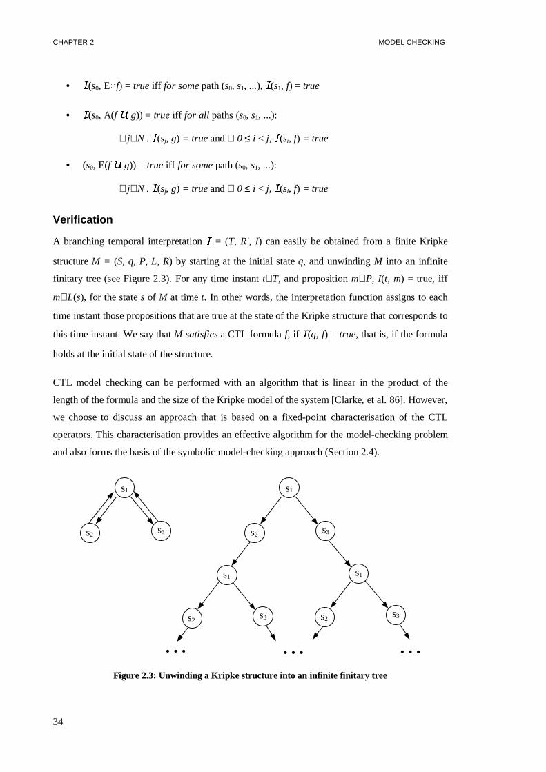
A branching temporal interpretationI = (T, R', I) can easily be obtained from a finite Kripke
structureM = (S, q, P, L, R) by starting at the initial stateq, and unwindingM into an infinite
finitary tree (see Figure 2.3). For any time instantt∈T, and propositionm∈P, I(t, m) = true, iff
m∈L(s), for the states of M at timet. In other words, the interpretation function assigns to each
time instant those propositions that are true at the state of the Kripke structure that corresponds to
this time instant. We say thatM satisfiesa CTL formulaf, if I(q, f) = true, that is, if the formula
holds at the initial state of the structure.
CTL model checking can be performed with an algorithm that is linear in the product of the
length of the formula and the size of the Kripke model of the system [Clarke, et al. 86]. However,
we choose to discuss an approach that is based on a fixed-point characterisation of the CTL
operators. This characterisation provides an effective algorithm for the model-checking problem
and also forms the basis of the symbolic model-checking approach (Section 2.4).
s1
s2s3
s1
s2
s1 s1
s2s3 s2
…… …
s3
s3
Figure 2.3: Unwinding a Kripke structure into an infinite finitary tree

CHAPTER 2 MODEL CHECKING
35
Let M = (S, q, P, L, R) be the Kripke model of the system, andPred(S) denote the lattice of
predicates overS, where each predicate is identified with the set of states inS that make it true,
and the ordering is set inclusion. Thus, the least element of the lattice is the empty set denoted by
false, and the greatest element is the set of all statesS denoted bytrue. A functional F from
Pred(S) to Pred(S) is called apredicate transformer. If we view each CTL formulaf as a
predicate identified with the states inM that satisfyf, then each of the basic CTL operators can be
characterised as a fixed point of a monotonic predicate transformer [Clarke, et al. 96b]. For
example, E◊p is characterised as the least fixed point of functionalZ [p ∨ E○Z], whereZ is a
variable that acts as a placeholder, i.e.Z gets substituted in (p ∨ E○Z) when the functional is
applied to a parameter.
For finite domains, least and greatest fixed points of monotonic functionals can be efficiently
computed [Clarke, et al. 96b]. The functional is applied in rounds until a fixed point is obtained:
the first round applies it tofalseor true for the least or greatest fixed point respectively, and each
new round applies it to the result of the previous round. Since the domainS is finite, this
procedure is guaranteed to terminate, in fact it will terminate after at most |S| rounds [McMillan
93].
This model-checking algorithm therefore computes, for a given Kripke structureM, and a CTL
formula f, the set of statesS1∈Swheref holds. ThenM satisfiesf if its initial stateq belongs toS1.
CTL model checking has also been extended to handle fairness constraints given as Büchi
acceptance conditions. In this context, model checking is restricted to fair computation paths, i.e.
paths along which each constraint holds infinitely often [Clarke, et al. 86, Clarke, et al. 96b].
2.2 Automata-theoretic methods
In automata-theoretic methods, the specification is given as an automaton. Then the system, also
modelled as an automaton, is compared to the specification to determine whether its behaviour
conforms to that of the specification. Several notions of conformance have been explored,
including language inclusion, equivalence, and refinement orderings [Clarke and Wing 96a].
Conformance with respect tolanguage inclusionconsists of checking that the language of the
automaton representing the system is contained in the language of the automaton representing a
system property. [Kurshan 94] describes how language inclusion can be checked forω-automata
(these are finite automata on infinite words, Büchi automata being an example of those). The
approach is similar to checking LTL properties by translating the LTL formulas into Büchi
automata, as presented in Section 2.1.1. In fact, the work of [Vardi and Wolper 86] on model

CHAPTER 2 MODEL CHECKING
36
checking LTL using automata has related the temporal and automata-theoretic approaches to
model checking.
Equivalence checkingconsists of comparing the model and the specification of the system with
respect to some equivalence relation [Cleaveland, et al. 93b, Fernandez 88, Fernandez, et al. 96].
Notions of equivalence that are often used in practice include observational and strong
equivalence, observational congruence [Milner 89], trace and failure-divergence equivalence
[Hoare 85], and branching equivalence [Glabbeek and Weijland 89]. Tools that take this
approach typically support several notions of equivalence. Designers can thus select the notion of
equivalence of interest, based on the semantics that they wish to attach to the state machines that
are compared.
In refinement orderings[Cleaveland, et al. 93b, Roscoe 94] (also known aspreorder checking),
specifications are treated as minimal requirements to be met by the system (the system is often
referred to asimplementationin this context). Specifications can then be partial, i.e. they may
contain “holes” – these are points where the system designer wants to allow freedom for the
implementation [Cleaveland, et al. 93b]. In this case, an implementationA needs to supply at
least the behaviour demanded by its specificationB, while adding detail to the parts that are
under-specified. We then say thatA is more defined thanB, or thatA refinesB, which establishes
an ordering relation between processes, referred to asrefinementor preorder. Refinement
checking algorithms proceed in a similar fashion to equivalence checking.
The idea of refinements gives rise to an approach to system development known assuccessive
refinements[Kurshan 94]. This is a methodology driven by the creation of a succession of
models of increasing detail, all the way to executable implementations. The model of each level
refines that of the previous level, and serves as a specification for the succeeding model. The
requirement is that if a modelM1 is a refinement of a modelM2, then it must be guaranteed that
M1 satisfies the properties that have been proven forM2. This permits verification of each
property in the simplest model where it can be defined [Kurshan 94].
2.3 Discussion
In general, programs are modelled as non-deterministic transition systems. The non-determinism
comes either from the modelling of concurrency by interleaving, or from the absence of
information about the behaviour of some component of the system or its environment [Wolper
95]. An unavoidable issue is how to handle in a logic the fact that, in non-deterministic models,
each state has multiple successors [Wolper 95].

CHAPTER 2 MODEL CHECKING
37
As seen, the branching approach to temporal logic deals with non-determinism explicitly, as the
model of time is a tree, where each node may have multiple successors. Formulas are interpreted
on the computation tree defined by the finite-state model of the program. Branching-time
operators are used to express the fact that something has to hold for some, or for all possible
futures. On the other hand, the linear approach handles non-determinism implicitly. A program is
viewed as a set of possible executions. Formulas are interpreted on program executions, which
evolve linearly in time.
Let us compare at this point the relative expressiveness of the various property specification
formalisms in model checking. We perform this in terms of the temporal logics LTL and CTL,
and of Büchi automata; these have efficient decision procedures and have been extensively used
in existing verification methods and tools.
There exist properties of CTL that cannot be directly expressed in LTL. For example, assume
CTL property A□E◊start, which states that regardless of what state the program enters, there
exists a computation leading back to the initial state of the program. Neither this property, nor its
negation can be expressed in LTL [Clarke, et al. 97]. On the other hand, a simple and often used
LTL formula □◊p, which states thatp must hold infinitely often in every program execution, is
expressed in CTL by the more complicated formula A□A◊p. CTL formulas tend to be longer and
more complicated, because branching operators must always precede linear ones.
Büchi automata have a number of advantages as compared to temporal logic. Firstly, they are
inherently capable of expressing eventuality and fairness assumptions. As a result, both the
system and its specification are defined in a syntactically uniform fashion. With LTL and CTL
model checking, Büchi acceptance conditions need to be introduced in the system model in order
to handle fairness [Aggarwal, et al. 90, Clarke, et al. 86, Kurshan 94]. An additional advantage of
Büchi automata is that they can express such properties as “p must hold at every even time
instant” (often referred to as unbounded sequentiality properties), which are not expressible in
the logics presented [Kurshan 94]. To conclude, the expressive power of Büchi automata is
strictly larger than that of LTL [Wolper 83]. As far as CTL is concerned, there are properties
expressible by automata that are not expressible in CTL, and vice versa.
In our approach, properties can be specified either as LTL formulas that are translated into Büchi
automata for verification, or directly as Büchi automata. This choice has been influenced by the
following factors:

CHAPTER 2 MODEL CHECKING
38
• Most properties that the average user of a model-checking tool needs to specify can be
expressed in all formalisms discussed. Therefore our choice of formalism is related more to
the usability of the formalism than to its relative expressiveness. With temporal logic
formalisms, the linear approach is natural when the properties are thought of as related to
executions of the program. The branching approach is well adapted when the properties are
thought of in terms of the structure of the program [Wolper 95]. We have found that it is
more intuitive, and consequently less error-prone, to express properties of programs in LTL.
• As compared to automata, logical notations may be more compact and usable in defining
properties. Admittedly, this advantage becomes less significant as more complicated
properties need to be expressed. On the other hand with automata, the system and its
properties are handled in a uniform way. The syntactic advantage of a logical notation may
also be offset through the use of a library of parameterised common properties. In general,
logical notations and automata both have their respective advantages. It is therefore a useful
feature for a method to accommodate both kinds of formalisms. This can be easily achieved
in the context of LTL model checking, as described in 2.1.1. The automata-theoretic
approach to LTL model checking has been efficiently implemented in a number of
approaches [Aggarwal, et al. 90, Holzmann 97]. Although a similar approach has been
proposed for model checking branching-time logics [Bernholtz, et al. 94], this approach is
not as well-established. Finally, as described in Chapters 4–6, the expression of properties as
automata is essential for the mechanisms that we have developed for model checking in the
context of CRA.
As far as building a system by successive refinements is concerned, we believe that, although
promising from a theoretical point of view, the approach is of limited practical interest. Besides
significantly restricting the choices of designers during system construction, one must understand
the concept well in order to use it correctly. Additionally, it is hard for a developer to gain
benefits early enough to be convinced to use the method.
In general, we believe that it is extremely optimistic to assume that a system can be built in a
provably correct fashion, proceeding formally all the way from specification to construction.
Rather, we view formal verification as a way of checking that the protocols designed and the
algorithms used for achieving a specific goal satisfy the properties required from them. The way
in which these will be implemented is the responsibility of the developer, who must be trusted in
turning the main design ideas into an efficient implementation. As a means, however, of bridging
the gap between design and implementation, our approach uses software architecture, as
described in Chapter 3. We believe that this is a practical trade-off between i) guiding the

CHAPTER 2 MODEL CHECKING
39
development of the system by restrictive formal rules to guarantee correctness and ii) proving
correctness for a model of the system that has no obvious links to the system implementation.
2.4 Symbolic representation
The model-checking algorithms discussed in previous sections suffer from the state explosion
problem. In the following sections, we discuss approaches for alleviating this problem (see
Figure 2.2).
Symbolic representationis based on representing the finite-state model of a system implicitly
[Coudert, et al. 89, McMillan 93]. The usual implicit representation is an efficient encoding of
Boolean functions known as Ordered Binary Decision Diagrams (OBDDs) [Bryant 92]. OBDD
representations have three main advantages: they are reasonably small for a large class of
interesting Boolean functions, they are canonical for a given ordering of the input variables, and
they can be directly manipulated to perform efficiently all basic Boolean operations [Kurshan
94].
0
a
c
b
d
1
0 1
0 1
0 1
0 1
1
0
a
b
c
dd
c
dd
b
c
dd
c
dd
0
0
00
0
1
00
0
1
1
1 1
1
1
1 1 1 1 1 1 11 0 0 0 0 0 0 0
0 0 0 1 0 0 0 1 0 0 0 1 1 1 1 1
Figure 2.4: Ordered binary decision tree and OBDD for (a∧∧∧∧b)∨∨∨∨(c∧∧∧∧d) with variable ordering a<b<c<d
An OBDD is similar to a binary decision tree, except that its structure is a directed acyclic graph
rather than a tree, and there is a strict order placed on the occurrence of variables as the tree is
traversed from the root to the leaves. More specifically, the OBDD representation for a Boolean
function f is obtained by reducing a related structure called ordered binary decision tree (see
Figure 2.4). To obtain the truth-value given specific values of the variables inf, one traverses the
binary decision tree from the root to the leaves. At each node, the value of the corresponding
variable determines which path will be taken: one descends the left/right child if the value of the
variable labelling the node is false/true (value 0/1), respectively. The variables in the tree occur

CHAPTER 2 MODEL CHECKING
40
in increasing order along any path from the root to the leaves. The binary decision tree is reduced
into an OBDD by combining any isomorphic sub-trees into a single tree, and eliminating any
nodes whose left and right children are isomorphic (see Figure 2.4).
The finite-state model of a system can be expressed in terms of OBDDs as follows. Each state is
encoded by an assignment of Boolean values to the set of state variables associated with the
system. If the state variables are not binary but range over a finite domainD, then an appropriate
binary encoding onD can be used. This process is made transparent to the user in tools that
support symbolic representation (e.g. SMV [McMillan 93]). The transition relation can thus be
expressed as a Boolean function in terms of two sets of variables, one set encoding the current
state, and the other encoding the new state. This function is represented as an OBDD.
Symbolic model checkingchecks temporal formulas directly on the OBDD representation of the
model of the system. The corresponding algorithm for CTL, for example, proceeds similarly to
the algorithm of Section 2.1.2. It uses OBDD representations for the transition relation and the
atomic propositions, and returns an OBDD representing the states of the system where the given
formula holds. All manipulations required by the algorithm – including comparison of OBDDs to
check whether the fixed point has been reached – can be performed efficiently on OBDDs. The
approach has been applied successfully for CTL model checking. However, LTL model-checking
and automata-theoretic approaches can also benefit from representing the model of the system
symbolically [Clarke, et al. 97, Fernandez, et al. 93, Kurshan 94].
To conclude, the symbolic approach avoids constructing the state graph of the concurrent system
explicitly [Clarke, et al. 96b, McMillan 93]. The issue is therefore no longer the size of the state
space but the size of the OBDD representation. As the latter captures some of the regularity in
state spaces, it has been possible to verify systems (hardware in particular) many orders of
magnitude larger than could be handled with an explicit representation of the state space [Burch,
et al. 90, Clarke, et al. 93b].
OBDD-based algorithms have not yet replaced explicit enumeration algorithms, as they do not
perform better in all cases [Kurshan 94]. This is mainly on account of the fact that the size of an
OBDD depends critically on the variable ordering. The problem of finding the ordering that
returns a minimal tree is NP-complete. Several heuristics have been developed for finding a good
variable orderingif such an ordering exists. However, there are Boolean functions that have
exponential size OBDDs foranyvariable ordering [Clarke, et al. 93a].

CHAPTER 2 MODEL CHECKING
41
2.5 On-the-fly verification
Reachability analysis is a verification technique that performs an exhaustive exploration of all
reachable states and transitions of a system. On-the-fly techniques are based on the observation
that in performing reachability analysis, it is not necessary to store the entire state graph of the
global system (or reachability graph). In fact, state explosion would make this impossible for
most systems of practical relevance. Rather, it is enough to simulate all possible transition
sequences that the system is able to perform. A classical depth-first search can be used to explore
the system “on-the-fly”, i.e. without storing the transitions that are taken during the search. This
reduces substantially the memory requirements [Godefroid, et al. 92].
For a depth-first traversal of the graph, the minimal storage requirement is that of the current path
explored. Such a search reduces memory requirements while still guaranteeing exhaustive state-
space exploration. However, the time needed to perform the verification may grow dramatically
due to the regeneration of already-visited states. At the other extreme lies a depth-first traversal
of the graph where states are stored once they have been visited. This reduces time requirements
to the minimum, while requiring the storage of all reachable states. However, for large
reachability graphs, it may be impossible to store all states. Various methods have been proposed
that attempt a trade-off between these two strategies.
In addition to storing the current path, state-space cachingcreates a restrictedcacheof selected
visited states [Holzmann 87a]. Initially, all visited states are stored in the cache, until it fills up.
When this happens, old states are gradually replaced with new ones. Several replacement
strategies are studied in [Holzmann 87a]. The effectiveness of state-space caching depends on the
size of the cache, but also on the structure of the state space. The latter is highly unpredictable,
which complicates the task of finding an optimal caching setup, whereas an unsuccessful setup
results in catastrophic increase of execution time [Holzmann 87a, Jard and Jéron 91]. As
mentioned, such explosion of run-time requirements is caused by multiple explorations of
unstored parts of the state space. [Godefroid, et al. 92] describe a method that reduces the number
of times that states are visited during the search, thus increasing the benefits obtained with state-
space caching. This is achieved by avoiding the exploration of interleavings of the same partial
ordering of statement executions that lead to the same state (see also Section 2.6.1).
When the problem size is prohibitive for exhaustive verification, thebit-state hashingor
supertracetechnique performs apartial search of the state space [Holzmann 88, Holzmann 95].
Visited states are stored in a hash tableH, whose size depends on the available memory. For each
states, a single bit with addressh(s) is used, whereh is a hash function returning bit-addresses in

CHAPTER 2 MODEL CHECKING
42
H. If the bit at addressh(s) has value 1, then the searching algorithm assumes thats has already
been visited. Since there is no collision detection, the search is partial. The coverage of the
algorithm can be significantly increased with a sequential bit-state hashing technique [Holzmann
95]. The technique consists of performing multiple runs with statistically independent hashing
functions, until the required coverage level is reached. This is not a problem, because the limiting
factor in reachability analysis is usually space rather than time.
Traditionally, reachability analysis has been used successfully for detecting errors such as
deadlock or unexercised code [Courcoubetis, et al. 92]. However, the applicability of reachability
analysis algorithms has been extended with the development of automata-theoretic model-
checking approaches. For example, as discussed in Section 2.1.1, LTL model checking can be
reduced to reachability analysis (although on a state space that is the product of the original state
space with the state space of the property automaton [Vardi and Wolper 86]). It is then possible
to provide algorithms for performing model checking “on-the-fly”.
[Courcoubetis, et al. 92] and [Godefroid and Holzmann 93] propose memory-efficient algorithms
for checking emptiness of Büchi automata in LTL model checking. These algorithms can be used
for performing on-the-fly verification, and are compatible with complexity-management
techniques such as bit-state hashing and state-space caching. [Gerth, et al. 95] propose an
algorithm that translates an LTL formula into a Büchi automaton, using a very simple depth-first
search. In this way, the protocol verification algorithm obtained constructs both the protocol and
the property automaton (and hence the product automaton) “on-the-fly” during a depth-first
search that checks for emptiness. More recently, algorithms have been developed for on-the-fly
model checking of branching-time logics [Bhat, et al. 95].
An “on-the-fly” approach can also be taken for checking behavioural equivalences and preorders.
[Fernandez and Mounier 91, Fernandez, et al. 92a] describe a technique which, in order to check
equivalence, performs reachability analysis on a particular synchronous product between the
LTSs compared. During the computation of this product, transitions to a specific sink statefail
may be introduced in the resulting state space. When any of the two systems is deterministic,
equivalence checking reduces to the reachability of the statefail in the product state space.
An advantage of on-the-fly verification is that it needs only proceed until an error is detected, in
which case a counterexample is generated to assist the designer with error correction. Often,
errors are discovered very early during the search, thus avoiding the exploration of the entire
state space. On the other hand, when the system is correct, the search covers the entire state

CHAPTER 2 MODEL CHECKING
43
space. The approach is therefore particularly suitable for early stages of design, which tend to
contain many errors [Kerbrat 94].
2.6 Reduction
Reduction techniques concentrate on building part of, or an abstraction of the state space of a
program, while fully preserving the capability to prove properties of interest. In this section we
describe the main approaches to state-space reduction.
2.6.1 Partial-order reduction
In most model-checking approaches, concurrency is modelled by interleaving, which is a major
factor contributing to state explosion. Partial-order reduction is based on the observation that in
concurrent systems, the total effect of a set of actions is often independent of the order in which
these actions occur. As a result, wasteful generation of all possible interleavings between such
actions can be avoided. Several methods based on this idea have been proposed, which explore a
reduced graph of the system while preserving properties of interest [Godefroid and Wolper 91,
Godefroid and Wolper 94, Holzmann, et al. 92, Peled 94, Valmari 93a].
Partial-order reduction methods perform aselectivesearch of the system state space. For each
states reached during the search, they compute a subsetT of the set of transitions enabled ats,
and explore only transitions inT. This is their difference with classical searches, which, for each
states reached during the search, explore all transitions enabled ats. Two main techniques have
been proposed in the literature for identifying these subsets; they are based on the computation of
persistent sets, andsleepsets [Wolper and Godefroid 93].
A persistent set Tfor some states contains transitions enabled ats, with the following
characteristic: any transition that is reachable froms by performing exclusively transitions not in
T is independentof (i.e. does not interact or affect) transitions inT (see [Wolper and Godefroid
93] for more details). One of the basic persistent set techniques is proposed by [Valmari 93a] and
is based on the computation ofstubborn sets. In the reduced exploration of the system state
space, only transitions in the stubborn set of each state are selected. It has been proven that the
execution of all remaining transitions can be postponed without affecting the verification results.
The aim is therefore for the stubborn set to be as small as possible, in order to achieve a larger
reduction of the state space. The algorithm described by [Valmari 93a] computes stubborn sets
during state-space exploration and can be performed “on-the-fly”.

CHAPTER 2 MODEL CHECKING
44
Thesleep-set technique exploits information about the past of the search. Used alone, it reduces
the number of transitions explored, but not the number of states. As mentioned in Section 2.5,
this is very useful when sleep sets are combined with state-space caching techniques [Godefroid,
et al. 92]. During depth-first search of the system graph, each states is associated with a sleep
set, which is a set of transitions that are enabled ins but will not be executed froms. Sleep sets
can be combined with persistent sets to further reduce the state space explored. Indeed, when the
persistent set technique cannot avoid the selection of independent transitions in a state, sleep sets
can avoid the exploration of multiple interleavings of these transitions [Wolper and Godefroid
93].
[Godefroid and Wolper 91] propose partial-order techniques for the verification of deadlock
freedom and safety properties. In this work, safety property checking is reduced to deadlock
detection, for which an efficient partial-order technique is described. More recent techniques
have been proposed that extend earlier work on partial orders and bring it to the full capabilities
of model checking. Some of these techniques perform model checking of LTL formulas that do
not contain the “next time” operator [Holzmann and Peled 94, Peled 94]. The technique
presented by [Godefroid and Wolper 94] can handle the full LTL logic, as well as some extended
logics. This approach uses automata-theoretic techniques that include extensions ofω-automata.
When combined with model checking, partial-order reduction is also tailored according to the
property that is being verified. It is usually the case that partial-order techniques attempt to
compute, mostly during the search, those parts of the state graph that are redundant and can be
skipped. However, [Holzmann and Peled 94] propose astatic reduction technique, where some
of the dependency relations between statements of a model are pre-computed, thus avoiding the
run-time and resource overhead that dynamic approaches inevitably introduce.
2.6.2 Compositional minimisation
The task of verification consists of establishing that a systemS satisfies some propertyf. Now
consider some semantic equivalenceR that preserves propertyf. ThenS satisfiesf iff S´ satisfies
f, whereS´ is the minimal state machine such that (S, S ) ∈ R. We say thatS´ is thequotientof S
with respect toR. The process of constructingS´ from S is calledminimisation. WhenR reflects
the application of an abstraction toS, thenS´contains fewer states thanS.
The technique of analysing the minimised state machine corresponding to some system rather
than the system itself, may in principle increase significantly the size of the systems that can be
analysed with given computer resources. Obviously, the objective is to obtain the minimised

CHAPTER 2 MODEL CHECKING
45
graphS´ without first generating the complete graph of the system.Compositional minimisation
provides a way of achieving this.
Assume a system described by a composition expression that groups together individual state
machines. Such an expression reflects a specific organisation of the system components in a
hierarchical structure. Compositional minimisation then performs minimisation in steps, from the
lowest to the highest level of the hierarchy. The composition expressions of each level define
which state machines must be composed in order to obtain state-machines of subsystems at that
level. The result of each composition is minimised. Several notions of equivalence can be used
with this approach, provided that the equivalence used is acongruencewith respect to the
operators in the composition expressions [Milner 89]. This is to ensure that components can
safely be substituted by their minimised versions in those expressions, without affecting the
result obtained.
In the process described above, the state graph for intermediate subsystems is constructed with
reachability analysis. Therefore, this approach of incremental composition and reduction is often
calledCompositional Reachability Analysis(CRA for short). [Valmari 93b] provides an excellent
description of some basic prerequisites for CRA methods:
• Combination of lower-level to upper-level systems.A CRA method needs to support
operations for i) composing component behaviour, ii) hiding details from component
behaviour that are not required in the system as a whole, and iii) renaming actions of
component interfaces for using components in different contexts.
• Equivalence notion. The equivalence notion used to simplify intermediate systems must
be strong enough to preserve the properties of interest, and weak enough to achieve a good
reduction of the state space. Moreover, the equivalence must be a congruence with respect to
the operations used to compose higher-level systems from lower-level ones.
• Reduction algorithm.The algorithm for reducing the size of intermediate subsystems
should be reasonably fast and produce as small state machines as possible. If the complexity
of minimisation is too high, an alternative reduction strategy should be considered that
attempts a balance between these two requirements.
The CRA approach is particularly suitable for analysing systems that are likely to evolve, as it
localises the effect of change. When changes are applied to a system, only the subsystems that
are affected by the changes need to be re-analysed. CRA techniques may be combined with
symbolic representation, but are not compatible with on-the-fly verification. This is because

CHAPTER 2 MODEL CHECKING
46
intermediate graphs for the systems need to be generated, rather than simply explored. On-the-fly
techniques may however be used at the last level of CRA, where the global system graph is
explored. Due to the reduction applied to intermediate subsystems, the global graph is expected
to be much smaller than the original graph of the system. The applicability of partial-order
reduction techniques in the context of CRA has not been investigated, to the best of our
knowledge.
One might expect that, with CRA, all intermediate state machines have a smaller size than the
state graph of the global system, and therefore the approach provides an efficient way of dealing
with state explosion. However, intermediate systems may explode faster than the initial system
itself. This phenomenon is known asintermediate state explosion. It is caused by the fact that
subsystems may contain many execution sequences that are unnecessary in the context of the
final system; these sequences will be forbidden when the subsystem is combined with the
remaining components of the system (referred to as thecontextor environmentof the subsystem).
Intermediate state explosion is particularly intense when components that are loosely coupled are
grouped together first. This may sometimes reflect bad structuring of the system, in which case a
better organisation might avoid the problem. However, as re-structuring of the system does not
always work, techniques that are more effective must be provided for addressing the problem.
Controlling intermediate state explosion
In order to address intermediate state explosion, both [Graf and Steffen 90, Graf, et al. 96], and
[Cheung and Kramer 96b] take the approach of usinginterfaces, which restrict the behaviour of
intermediate subsystems based on their context. An interface is a process representing a set of
authorised execution sequences that can be performed by the subsystem in the specific
environment. The more detailed the interface, the more it restricts the behaviour of the
subsystem, thus avoiding the occurrence of intermediate state explosion. An interface iscorrect
if its inclusion in the generation of the global system does not modify this system’s behaviour.
Interfaces can beautomatically generatedor user-specified. Automatically generated interfaces
are derived algorithmically, by procedures that guarantee their correctness. However, although
automatically generated interfaces can safely be introduced into the system, they may not restrict
the behaviour of intermediate subsystems sufficiently [Cheung and Kramer 96b]. User-specified
interfaces can provide an additional amount of detail. These are interfaces that system developers
specify based on their knowledge of the system. Even though they are expected to be correct in
the general case, they are but “guesses” of the context behaviour. Therefore, a method needs to

CHAPTER 2 MODEL CHECKING
47
be provided to guarantee that, in the presence of such interfaces, the behaviour of the system
remains unaltered.
In [Graf and Steffen 90, Graf, et al. 96], a technique is proposed that allows user-specified
interfaces to be used in CRA. Processes are modelled as LTSs and are combined with a CSP-like
composition operator || [Hoare 85]. The method extends LTSs with anundefinednesspredicate.
This predicate consists of pairs (s, A), wheres is a state in the LTS, andA is a set of actions
which, when executed froms, would allow the LTS to enter an undefined state. During CRA,
every subsystemS for which an interfaceI is provided is substituted byΠI(S). ΠI(S) is the
projection ofS||I on S, with one difference: whenever at some stateq, S can perform a transition
with actiona that is stopped byI, then (q, a) is inserted in the undefinedness predicate ofΠI(S).
ΠI(S) can be constructed in time proportional to the product of the number of transitions ofP and
I. Emptiness of the undefinedness predicate of the global LTS thus constructed guarantees
correctness of all interfaces introduced. Otherwise, some of the interfaces introduced are
incorrect, and therefore the LTS cannot be used for verification.
[Cheung and Kramer 96b] present a similar approach fordeterministicuser-specified interfaces.
They introduce aninterface theoremthat provides a number of sufficient conditions for an
interface to be correct. In their approach, LTSs are extended with an error stateπ. Each user-
specified interfaceI is automatically madecompletewith respect to its alphabet by substituting
missing transitions with transitions toπ. The resultI´ of the transformation is called theimage
interface. During CRA, if an interfaceI is provided by the user for a subsystemS, then S is
composed with the image interfaceI´. In this way, all transitions ofS that are stopped byI in S||I,
become transitions to theπ state inS||I´. If the π state is unreachable in the global graph of the
system, then the conditions of the interface theorem are satisfied, and therefore the interfaces
introduced are correct. The approach is however conservative; although no incorrect interface is
used for verification, there is no guarantee that a correct interface will not be rejected. This is
because the interface theorem provides conditions that aresufficient but not necessaryfor a
correct interface. In Chapter 5 (Section 5.1.2) we prove that the interface theorem can be
reformulated in a way that makes its conditions both sufficient and necessary.
The above approaches for dealing with user-specified interfaces have a common characteristic:
they do not require a separate proof of correctness for these interfaces (as is the case for [Shurek
and Grumberg 90], for example). More specifically, incorrect interface specifications never lead
to incorrect proofs. They may only prevent the successful verification of a valid statement.

CHAPTER 2 MODEL CHECKING
48
Even with a good knowledge of the system, users may not always be able to provide suitable
interfaces. To this aim, [Cheung and Kramer 96b] have developed an algorithm for generating
interfaces automatically. For a subsystemP, the algorithm applies a simple reduction on
individual LTSsLi in the context ofP. For eachLi, the reduction roughly consists of deleting the
transitions labelled with actions that do not belong toP. If a reducedLi is non-deterministic, it is
transformed into an equivalent deterministic one, and the resulting LTS is minimised. The
interface forP is the parallel composition of the deterministic LTSs obtained by this procedure.
Interfaces thus constructed satisfy the conditions of the interface theorem, and are therefore
correct by construction. The complexity of the algorithm is dominated by the procedure for
converting non-deterministic LTSs into deterministic ones. This procedure is exponential in the
size of the non-deterministic LTS. The authors report that in practice, the computational effort of
performing such transformations in the context of CRA is usually small.
10a
b
Ia
0
21
a
b
a
P
1,1
0,12, 0
b
a
a
P||I´
0, 0
a
10a
b
I ´a
πb
Figure 2.5: Interface I increases the size of subsystemP
In the techniques proposed by [Cheung and Kramer 96b], the behaviour of intermediate
subsystems may be expanded with the use of interfaces, although the latter are deterministic (see
Figure 2.5). The approach of [Graf, et al. 96] avoids this problem as follows: for a subsystemP
and an interfaceI, rather than simply composingP with I, it projects the behaviour ofP||I on P.
For example, the behaviour of subsystemP in Figure 2.5 remains unchanged by interfaceI. The
techniques of [Cheung and Kramer 96b] can easily incorporate this idea, in order to avoid
increasing the size of intermediate subsystems when interfaces are used.
[Yeh 93a] proposes a technique where constraints are not specified as separate interface
processes, but throughSLEEPP, WAKEP, and ACTIVATE P transitions (the indices represent
identities of processes). Such transitions are introduced by the developer in the specifications of
individual processes of the system. ASLEEPP transition indicates the transition of processP to a
sleeping state. WhenP is composed with other processes, the execution of any action enabled at
a sleeping state leads to aTRAP state, which is an error state. It denotes that the behaviour pruned

CHAPTER 2 MODEL CHECKING
49
out from P with the SLEEPP mechanism does not correspond to context constraints imposed by
the environment of the process.SLEEPP transitions are nullified byWAKEP transitions and are
propagated to composite processes withACTIVATE P transitions. Note that such transitions can be
combined only if they have a matching index. Constraints imposed by this mechanism are correct
unless theTRAP state is reachable in the global graph of the system The main disadvantage of
this method is that the composition operator is no longer associative. As a result, explicit
description of the order in which the system is to be composed must be provided with the
specifications. Moreover, as separation of concerns enforces clearer modelling, it is preferable
for context constraints to be specified separately from component behaviour.
[Krimm and Mounier 97] adopt the approach proposed by [Graf, et al. 96], but in the framework
of LOTOS parallel composition. They define asemi-compositionoperator, which restricts the
behaviour of a process with respect to some interface, for expressions that consist of the LOTOS
operator ||G (P ||G Q is the LTS obtained by synchronisation on the actions that belong toG, and
interleaving of the other actions – operator ||G is not associative). In their approach, the
behaviour corresponding to any sub-expression in a composite expression can be restricted
according to the behaviour of any sub-expression in its environment, with the use of semi-
composition. Well-defined rules control what makes up the “environment” of sub-expressions.
Interfaces introduced in this way are guaranteed to be correct, although they often prove
insufficient. User-specified interfaces are therefore also supported. The correctness of such
interfaces is checked according to the method proposed by [Graf, et al. 96].
Experience
Promising results have been reported from the use of CRA to generate the state space for a well-
structured concurrent system. [Sabnani, et al. 89] describe an experiment, where CRA is applied
to the Q.931 protocol. The intermediate state spaces generated never exceed 1,000 states
although the global state space given by traditional reachability analysis of the protocol contains
over 60,000 states. Similar observations are made by [Valmari93b] and by [Tai and Koppol 93].
From now on, we will use the terminology introduced by [Graf and Steffen 90] for discussing
results obtained with CRA. According to this, the size of the original state space of a system is
referred to as itsapparent complexity, the size of the minimised state space as itsreal
complexity, and the size of the maximal transition system encountered by CRA as itsalgorithmic
complexity.

CHAPTER 2 MODEL CHECKING
50
[Yeh 93a] describes the case study of a remote temperature sensor system. By using CRA
extended with theSLEEP/WAKE/ACTIVATE mechanism, the algorithmic complexity is a few
hundred states. Although the apparent complexity is not computed, its estimated size (obtained as
the product of component sizes) is of the order of 1016 states. Various other case studies
demonstrate the advantages of using such an approach.
[Cheung and Kramer 96b] usecontextualCRA (i.e. CRA enhanced with the use of interfaces) to
analyse several systems. They show that the algorithmic complexity obtained by their technique
is often significantly lower than the algorithmic complexity of CRA. For a client/server system
the latter grows exponentially with the number of clients included, whereas this problem is
avoided in contextual CRA. Similar results are reported from the case study of a gas station
example and a distributed track control system [Cheung and Kramer 94a]. In these experiments,
contextual CRA also considerably reduces the apparent complexity of a system.
[Krimm and Mounier 97] give experimental results obtained from applying their technique on
two realistic LOTOS examples: an atomic multicast protocol that requires user-specified
interfaces, and a leader election algorithm that is handled automatically. They have performed
their experiments using the CADP toolbox [Fernandez, et al. 96]. In this way, they have been
able to compute the apparent complexity of very large systems by using a symbolic generation
method (based on BDD encoding). Their examples show that their approach largely avoids the
apparent complexity of the system, while sometimes remaining close to its real complexity. In
the case study of the atomic multicast protocol, none of the intermediate LTSs exceeds a million
states, and the resulting LTS is approximately 200,000 states, which is manageable for
verification purposes. The generation process completed in a few hours on a SUN SS 20
workstation. The application to this example of a symbolic generation method leads to an LTS of
about 200 million states (represented by a BDD) obtained in one week of computations using the
same workstation. For these two examples, compositional minimisation also achieves better
results than on-the-fly verification and symbolic minimal model generation [Fernandez, et al.
93]. This, however, is not true of all examples that the authors have considered, which only
confirms the observation that no single verification method can perform best in all cases.
2.6.3 Abstraction
Most reduction strategies rely on applying some kind of abstraction to the system under analysis.
In fact, compositional minimisation can also be viewed as an abstraction technique: it abstracts
details from the system behaviour, based on a description of the system structure and the
specification of how its components interact.

CHAPTER 2 MODEL CHECKING
51
Localisation reductionis an automated, property dependent reduction technique proposed by
Kurshan [Kurshan 94]. It is applied dynamically when checking language inclusion in automata-
theoretic verification methods (see Section 2.2). Language inclusion properties are preserved
when additional processes are included in a model. The algorithm thus initially considers an
abstraction of the system containing only a subset of the system processes, and is recursively
applied to successive approximations of the system until inclusion is proven, or a
counterexample is returned that corresponds to a legal execution of the system. The selection of
processes that are included in each approximation is based on a directed graph of dependencies
among the processes of the system.
A similar approach is proposed by [Bharadwaj and Heitmeyer 97] for checking invariance
properties on abstractions of a system. Such abstractions are generated directly from the system
specification by eliminating state variables that do not affect the property of interest. The abstract
system contains only those variables that belong to the reflexive transitive closure of the set of
variables that appear in the property, under the dependency relation between system variables.
For programs with data-dependent behaviour, [Clarke, et al. 94] propose to perform model
checking onapproximationsof their state spaces, when these state spaces are very large (or
possibly infinite). Approximations are based on mapping the sets over which program variables
range, onto sets of abstract values. They are constructed directly from the text of a program,
without first building the original transition system. This approach is closely related to abstract
interpretation techniques[Cousot and Cousot 77] that have traditionally been applied to studying
compile-time analyses of programs. [Cousot and Cousot 99a] also suggest ways in which ideas
from abstract interpretation may be used to enable the application of reachability analysis to
finite- and infinite-state systems.
Other approaches to abstraction include exploitingsymmetriesin the system for state-space
generation [Ip and Dill 93] and for model checking [Clarke, et al. 96c]. In general, abstraction
techniques for programs with data-dependent behaviour are less applicable to concurrent
systems, where, as mentioned, the focus is on theinteractionsbetween processes.
2.7 Compositional reasoning
Compositional reasoning(or compositional verification) exploits the natural decomposition of a
complex system into simpler components. Properties of system components are verified first.
These properties are then combined to deduce properties of the global system. Obviously, the
approach does not suffer from state explosion since it does not require the construction of the

CHAPTER 2 MODEL CHECKING
52
system state space. An issue that arises however is that often, properties of subsystems are
satisfied only when specific assumptions are made on their environment. An approach proposed
for dealing with this issue is to use interface processes that model the environment of the
subsystem [Clarke, et al. 89] (in a similar way to CRA techniques – Section 2.6.2).
A great amount of research has been devoted to compositional reasoning – after all, the approach
provides the most promising attack to state explosion [Abadi and Lamport 95, Alur and
Henzinger 95, Grumberg and Long 94, Manna and Pnueli 95, Pnueli 85]. Kurshan’s localisation
reduction (Section 2.6.3) can be considered a simplified compositional verification method, since
it attempts to prove global system properties by checking if they are satisfied by some component
of the system. The advantage of localisation reduction is that it can be automated.
In general, it is a complicated task to decompose properties of the global system into local
properties of its components. Moreover, it must be proven that such decompositions are correct,
i.e. that the satisfaction of local properties of subsystems implies the satisfaction of some global
property by the system. The approach needs to be supported by automated tools to a high degree
in order to become widely usable by software engineers. As [Kurshan 94] reports, “finding useful
heuristics to determine decompositions of global system properties into local properties of
subsystems is one of the foremost open problems in the field”. [Clarke and Wing 96a] make a
similar observation: “we need to develop more efficient ways for decomposing a computationally
demanding global property into local properties whose verification is computationally simple”.
2.8 Discussion
Software architecture describes the organisation of a system in terms of its components and their
interactions. In general, the software architecture of a system has a hierarchical structure, with
primitive components at the leaves, and composite components at the non-leaf nodes of the
hierarchy. Software architecture concentrates on the interfaces and interconnections of
components, and is not concerned with their functionality. When the functionality of primitive
components is provided by the designer, the architecture describes the exact way in which these
components are put together, in order to form a complete system. For model checking, the
functionality is described in terms of finite-state machines, and for construction, in terms of some
programming language.
Software architecture can therefore be used tointegrate the various phases of software
development. Such integration significantly contributes to the usability of methods and tools, as
discussed in Section 1.2. In our approach, analysis of a system is based on its software

CHAPTER 2 MODEL CHECKING
53
architecture. Compositional minimisation and compositional reasoning then become a natural
choice for state explosion control, as they can effectively exploit the decomposition of a system
into a hierarchy of components. This has motivated our use of CRA to generate the finite-state
model of a system, as described in Chapter 3. Our work therefore focuses on developing model-
checking strategies in the context of CRA. An additional motivation for taking this approach is
that it can easily accommodate compositional reasoning, a direction in which we wish to extend
our work.
2.9 Model-checking tools
A large number of model-checking tools have been developed over the years. This section
provides an overview of some well-known model checkers.
CADP
CADP (CÆSAR – ALDÉBARAN Development Package) [Fernandez, et al. 96, Fernandez, et al.
92b] is a verification toolbox for the design and verification of communication protocols and
distributed systems, specified in the ISO language LOTOS [ISO 88]. The semantic model is
based on LTSs. CADP accepts low-level specifications in terms of LTSs, and also supports
intermediate formats that allow verification of protocol descriptions written in other languages
such as SDL [CCITT 93]. The toolbox contains several closely interconnected components
accessible through a graphical user-interface. The functionalities offered include interactive or
random simulation, partial and exhaustive deadlock detection, verification of behavioural
specifications with respect to various equivalence relations, as well as verification of branching-
time temporal logic specifications in the logic XTL (eXecutable Temporal Language). LTSs may
be represented either explicitly or implicitly in terms of BDDs. On-the-fly verification can be
applied, and so can compositional state-space generation. Minimisation is supported with respect
to several equivalence relations. Intermediate state explosion is addressed by the use of the semi-
composition operator for composing interfaces with intermediate subsystems [Krimm and
Mounier 97]. A number of case studies have been performed with the CADP toolbox, including
several industrial applications [Chehaibar, et al. 96, Korver 96, Pecheur 97, Sighireanu and
Mateescu 97].
Concurrency Workbench
The Concurrency Workbench [Cleaveland, et al. 93b] is a tool that incorporates several
verification strategies. A system is modelled as a CCS process [Milner 89]. Processes are then
interpreted as LTSs for verification purposes. The tool supports three different approaches to

CHAPTER 2 MODEL CHECKING
54
verification. Firstly, it checks behavioural equivalence between the LTS of the system and that of
its specifications. Various types of equivalence are supported, including Milner’s strong and
observational equivalence [Milner 89], trace, and failure equivalence [Hoare 85]. LTS
minimisation can also be performed with respect to these notions of equivalence. Although
minimisation is a facility provided by the tool, compositional state-space generation is not
mentioned as a possibility in [Cleaveland, et al. 93b], nor is any attention given to the problem of
intermediate state explosion.
Secondly, preorder checking can be performed between the system and its specifications.
Thirdly, the tool supports model checking of specifications written in a modal logic based on the
propositionalµ-calculus. Theµ-calculus is strictly more expressive than CTL and can also
express a variety of properties of transition systems, such as reachable state sets, state
equivalence relations, and language containment between automata [McMillan 93]. However,
formulas in this logic are unintuitive and difficult to understand [Cleaveland, et al. 93b]. For this
reason, the tool offers the facility of user-defined macro identifiers. In this way, users are able to
code intuitively well-understood operators as macros. The model-checking algorithm has
complexity that is exponential in the length of the formula checked, although for special classes
of formulas it is well-behaved. A linear-time algorithm has been proposed for a particular
subclass of the logic, called “the alternation free modalµ-calculus” [Cleaveland and Steffen 93c].
The NCSU Concurrency Workbench [Cleaveland and Sims 96a] is an extension of the
Concurrency Workbench. Finally, theConcurrency Factory [Cleaveland, et al. 96b] can be
viewed as a next-generation Concurrency Workbench, with a focus on usability. It allows non-
experts to design concurrent systems using GCCS, a graphical version of the process algebra
CCS.
COSPAN
Cospan [Hardin, et al. 96] takes the automata-theoretic approach to verification. It performs this
by checking inclusion of the language of the system in that of its desirable properties. The native
language is S/R (selection/resolution) but interfaces have been written for the commercial
hardware description languages Vérilog [Thomas and Moorby 98] and VHDL [IEEE 87], as well
as the CCITT-standard protocol specification language SDL [CCITT 93]. The semantic model is
founded onω-automata. In general, a system consists of a collection of such automata. To
facilitate property specification asω-automata, a library of parameterised automata is provided.
Counterexamples are returned when property violations are detected in a system. COSPAN can
use either symbolic (BDD-based) or explicit state-enumeration algorithms. The latter invoke

CHAPTER 2 MODEL CHECKING
55
caching and bit-state hashing options (as related to “on-the-fly” verification), as well as
minimisation algorithms. Several other reduction strategies are supported such as automated
localisation reduction, symmetry reduction, and user-defined homomorphic reduction (based on
the idea of abstract interpretation). COSPAN also supports top-down design development
through successive refinements.
FC2TOOLS
FC2TOOLS (the next-generation AUTO/GRAPH) [Bouali, et al. 96] is a verification tool-set that
supports graphical specification of concurrent systems. Reachability analysis, minimisation,
equivalence checking, and model abstraction can be performed on automata represented either
symbolically or explicitly. Moreover, compositional minimisation can be applied on a
hierarchical network of processes, although intermediate state explosion is not addressed. The
tool-set also supports the specification of properties in terms of automata, and implements on-
the-fly techniques for checking them.
FDR
FDR [Roscoe 94, Roscoe 98] is a tool based on the theory of CSP [Hoare 85]. FDR establishes
whether a property holds for a system, by checking that the system refines its property in the
traces, failures, or failures-divergences model. The standard model used is that of failures-
divergences, hence the name of the tool (Failures-Divergence Refinement). Both the system and
the property are specified in a machine-readable version of CSP, and their specifications are
translated into finite LTSs. For checking refinement, the property LTS is normalised before
model checking is applied. This can be a problem, as normalisation may increase the size of an
LTS exponentially. Additionally, a system can be developed by a series of stepwise refinements,
starting with a specification process and gradually refining it into an implementation. Finally,
FDR supports compositional minimisation, where intermediate systems can be simplified with a
variety of compression techniques.
SMV
SMV [McMillan 93] is a tool for checking finite-state systems against specifications in the
temporal logic CTL. It supports a flexible specification language and uses an OBDD-based
symbolic model-checking algorithm for efficiently checking whether CTL specifications are
satisfied by the system. The tool has been used to verify several industrial designs such as the
Futurebus+ and the Gigamax protocols [Clarke, et al. 93b, McMillan 93].
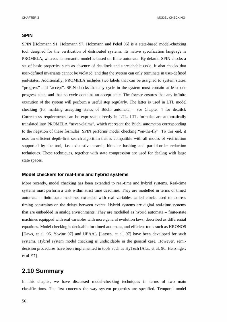
CHAPTER 2 MODEL CHECKING
56
SPIN
SPIN [Holzmann 91, Holzmann 97, Holzmann and Peled 96] is a state-based model-checking
tool designed for the verification of distributed systems. Its native specification language is
PROMELA, whereas its semantic model is based on finite automata. By default, SPIN checks a
set of basic properties such as absence of deadlock and unreachable code. It also checks that
user-defined invariants cannot be violated, and that the system can only terminate in user-defined
end-states. Additionally, PROMELA includes two labels that can be assigned to system states,
“progress” and “accept”. SPIN checks that any cycle in the system must contain at least one
progress state, and that no cycle contains an accept state. The former ensures that any infinite
execution of the system will perform a useful step regularly. The latter is used in LTL model
checking (for marking accepting states of Büchi automata – see Chapter 4 for details).
Correctness requirements can be expressed directly in LTL. LTL formulas are automatically
translated into PROMELA “never-claims”, which represent the Büchi automaton corresponding
to the negation of these formulas. SPIN performs model checking “on-the-fly”. To this end, it
uses an efficient depth-first search algorithm that is compatible with all modes of verification
supported by the tool, i.e. exhaustive search, bit-state hashing and partial-order reduction
techniques. These techniques, together with state compression are used for dealing with large
state spaces.
Model checkers for real-time and hybrid systems
More recently, model checking has been extended to real-time and hybrid systems. Real-time
systems must perform a task within strict time deadlines. They are modelled in terms of timed
automata – finite-state machines extended with real variables called clocks used to express
timing constraints on the delays between events. Hybrid systems are digital real-time systems
that are embedded in analog environments. They are modelled as hybrid automata – finite-state
machines equipped with real variables with more general evolution laws, described as differential
equations. Model checking is decidable for timed-automata, and efficient tools such as KRONOS
[Daws, et al. 96, Yovine 97] and UPAAL [Larsen, et al. 97] have been developed for such
systems. Hybrid system model checking is undecidable in the general case. However, semi-
decision procedures have been implemented in tools such as HyTech [Alur, et al. 96, Henzinger,
et al. 97].
2.10 Summary
In this chapter, we have discussed model-checking techniques in terms of two main
classifications. The first concerns the way system properties are specified. Temporal model

CHAPTER 2 MODEL CHECKING
57
checking and automata-theoretic model checking have been described, as well as the way in
which automata-theoretic approaches to temporal model checking relate the two. These
approaches are expressive enough to cover most types of properties that software engineers
usually need to express. The specific formalism to be used thus becomes a matter of preference.
Our approach supports specifications expressed either as LTL formulas or as Büchi automata.
The advantage is that, while the model-checking algorithms are the same for both formalisms,
the designer may select whichever is more intuitive or compact.
The second classification is related to techniques developed to address state explosion, i.e.
symbolic representation, on-the-fly verification, reduction, and compositional reasoning.
Particular emphasis has been placed on reduction by compositional reachability analysis (CRA),
in the context of which intermediate state explosion and ways of controlling it have been
described. Both CRA and compositional reasoning advocate a divide-and-conquer strategy, a
well-known and generic approach for solving large instances of problems. The idea is natural, in
particular because recent systems design techniques tend to promote hierarchical approaches.
In general, there is benefit in combining techniques for achieving better results. State explosion is
an inherent limitation of model checking and, as a result, no single technique is expected to be
efficient for all kinds of systems. This is also reflected by the fact that most of the existing
model-checking tools support several approaches to model checking. It is important to build on
experience in order to determine what kinds of analyses are appropriate for what kinds of
systems.

58

59
Design & Analysis 33.1 SOFTWARE ARCHITECTURE INDARWIN 59
3.2 MODELLING BEHAVIOUR 61
3.3 ASSOCIATING BEHAVIOUR WITH SOFTWARE ARCHITECTURE 66
3.4 COMPOSITIONAL REACHABILITY ANALYSIS 75
3.5 RELATED WORK 82
3.6 SUMMARY 84
To increase the usability of analysis techniques, particular emphasis needs to be placed on the
integration of analysis with other activities of software development. Methods that operate in
isolation may discourage potential users who are burdened with establishing a connection, and
achieving consistency, between the activities supported by these methods. Moreover, information
that is relevant to various phases of system development should ideally need to be provided once,
and be available in the appropriate form for all related activities. This requires the integration not
only of software development methods, but also of the tools that support them.
In TRACTA, the basic structure of a system is described in the Darwin architecture description
language. As Darwin advocates a modular and incremental approach to system development, we
follow a similar approach for behavioural modelling and analysis. This chapter proposes a
compositional model for system behaviour. The structural description of the system can thus be
exploited directly for modelling and analysis. Within this framework, compositional reachability
analysis provides a natural and effective way of dealing with state explosion. The proposed
approach is illustrated by a familiar educational example.
3.1 Software architecture in Darwin
Software architecture has been identified as a promising approach to bridge the gap between
requirements and implementations in the design of complex systems [Kramer and Magee 97,
Magee, et al. 97]. Software architecture describes the organisation of a system in terms of its
components and their interactions. It emphasises a separation of concerns; descriptions of
component structure and of component functionality are separate but related activities of
software development.

CHAPTER 3 DESIGN & ANALYSIS
60
Darwin [Magee, et al. 95] is an architecture description language (ADL) that supports a
component-based approach to program structuring. Acomponentis the unit of structure. A
component hides its behaviour behind a well-defined interface.Interfaces are points of
interaction of the component with its environment (i.e. other components in the system), and
represent services that the component provides or requires. Programs are constructed by creating
instancesof componenttypes and binding their interfaces together. Component types may
themselves have substructure. The general structure of a Darwin program is therefore a tree in
which the non-leaf nodes arecomposite components, and the leaves areprimitive components. A
primitive component has no substructure, and expressesbehaviouras opposed tostructure. The
structure of a composite component defines its behaviour based on that of its sub-components. A
composite componentencapsulatesall interactions among its sub-components that are not
connected to its interface.
Behavioural View Service View
Structural View
Analysis Construction/implementation
Figure 3.1: Common structural view with service and behavioural views
Darwin is sufficiently abstract to support multiple views. In this way, software architecture
describes the basic structure behind each view of the system during development
[Giannakopoulou, et al. 99a]. This structure can be enriched with behaviour specifications for
analysis (behavioural view) and service implementations for construction (service view), as
illustrated in Figure 3.1. For example, in the basic structure of the program, component interfaces
are simply sets of names that refer to actions or events shared between bound components. In the
service view these names correspond to services, for which the system designer needs to specify
whether they are provided or required by the component. In essence, the architecture describes
the way in which individual component specifications or implementations can be put together, in
order to obtain a system with desirable characteristics.
Darwin has both a textual and a graphical syntax, with appropriate tool support. The Software
Architect’s Assistant (SAA) [Ng, et al. 96] is a visual environment for the design and

CHAPTER 3 DESIGN & ANALYSIS
61
development of distributed programs using Darwin architectural descriptions. Facilities provided
include the display of multiple integrated graphical and textual views, a flexible mechanism for
recording design information and the automatic generation of program code and formatted
reports from design diagrams. The SAA interacts with the Darwin compiler to generate system
instances from a software architecture. As discussed, systems thus described typically have a
hierarchical structure.
Darwin has been used extensively for specifying the structure of distributed systems and
subsequently directing their construction [Magee, et al. 95, Magee, et al. 94, Magee and Kramer
96]. Similarly, software architecture can be used to direct system modelling and analysis
[Giannakopoulou, et al. 98b, Magee, et al. 98]. In the following, we present the relation between
software architecture and analysis, as established by our approach.
3.2 Modelling behaviour
We use finite labelled transition systems (LTS) to model the behaviour of communicating
processes in a distributed program. An LTS contains all the reachable states and executable
transitions of the process. The model has been widely used in the literature for specifying and
analysing distributed programs [Clarke, et al. 89, Ghezzi, et al. 91, Kemppainen, et al. 92,
Rabinovich 92, Valmari 92]. Appendix A provides a formal description of the LTS model and its
operators. In this section, we present the model in an informal but intuitive way.
3.2.1 Labelled transition systems
Let Statesbe the universal set of states,Act be the universal set of actions, andActτ=Act∪{ τ},
whereτ is used to denote an action that is internal to a subsystem, and therefore unobservable by
its environment. A finite LTSP is a quadruple⟨S, A, ∆, q⟩ where:
• S⊆ States isa finite set of states;
• A = αP ∪ { τ}, whereαP ⊆ Act denotes the communicatingalphabetof P;
• ∆ ⊆ S×A×S, denotes a transition relation labelled with elements ofA;
• q ∈ S indicates the initial state ofP.
We say thatP is deterministiciff ∀s, s , s ´∈S: ((s, a, s)∈∆ ∧ (s, a, s´)∈∆) ⇒ s = s ´, otherwise
it is non-deterministic. The term “LTS” will be used to refer tofinite LTSs, as we only deal with
such systems in our work.

CHAPTER 3 DESIGN & ANALYSIS
62
As an example, consider the following LTS model of a lamp:
Lamp = ⟨{0,1},{switch_on,switch_off},{(0,switch_on,1),(1,switch_off,0)},0 ⟩.
Figure 3.2 represents this LTS graphically. States0 and1 correspond to the lamp being off and
on, from which the lamp can be turned on and off respectively, by performing the actions
switch_on andswitch_off . Note that the names assigned to the states of an LTS act simply as
identifiers for those states, and do not carry any meaning (see Appendix A.5). Therefore, an LTS
is not modified if its states are renamed. The convention used in our diagrams is that states are
numbered with integers, where zero identifies the initial state.
A trace of an LTS P is a sequence of observable actions thatP can perform starting from its
initial state. We denote the set of possible traces ofP astr(P). Traces are denoted as sequences of
actions separated by commas, and enclosed in angular brackets. For example, one possible trace
of Lamp is: <switch_on,switch_off,switch_on> , whereas <switch_off,switch_on> does not
belong totr(Lamp) becauseswitch_off cannot be performed at the initial state ofLamp.
Lamp
switch_on
switch_off
0 1 Student
switch_on
switch_off
sleep read
0 1 2
Lamp_Studswitch_on read
switch_off
sleep
sleep
0 1 2 3 4
Figure 3.2: LTS models of a lamp and a student, and LTS of their joint behaviour
Composition
We denote that two LTSsP and Q run in parallel by “P||Q”, where “||” is the parallel
compositionoperator.P||Q is an LTS that models the joint behaviour ofP andQ. The alphabet of
P||Q is αP∪αQ, and its states can be viewed as pairs of states: state (p, q) reflects the fact thatP
is in statep and Q is in stateq. In the joint behaviour ofP and Q, any of the two LTSs can
perform a transition individually, so long as the action that labels that transition is not shared

CHAPTER 3 DESIGN & ANALYSIS
63
with the alphabet of the other LTS. Shared observable actions have to be performed
simultaneously. Transitions onτ are never synchronised, since they representlocal (and therefore
internal) behaviour.
Figure 3.2 illustrates the LTSLamp_Stud=Lamp||Student of the joint behaviour ofLamp and
Student . The states {0,1,2,3,4} of Lamp_Stud represent the composite states
{(0,0),(1,2),(1,1),(1,0),(0,1)} , respectively. We see that inLamp_Stud , the student is not
allowed to performswitch_off multiple times before performingsleep , which Student may
wish to do when in its local state1. Moreover, if the student sleeps without performing
switch_off , Lamp_Stud enters state3 (corresponding to composite state(1,0) ), which is a
deadlock state. In this state, the student wishes toswit ch_on the light, but the only action
available byLamp is switch_off . As bothswitch_on and switch_off are shared between the
two LTSs, neitherStudent , nor Lamp can perform them in isolation.
The parallel composition operator is both commutative and associative. The order in which LTSs
are composed is therefore insignificant. As described, LTSs communicate by synchronisation on
actions that their alphabets share, with interleaving of the remaining actions. Modelling
interacting processes with LTSs is therefore sensitive to the selection of action names.
Similarly to CSP [Hoare 85], the LTS parallel composition operator has broadcast semantics.
Broadcast communicationallows any number of processes to simultaneously participate in a
transition. In such a setting, it is easy to model a process that monitors the behaviour of a group
of communicating processes, by sharing actions in their alphabets, and executing jointly with
them. In TRACTA for example, “monitoring” processes are introduced to check that a system
satisfies its desired properties (as discussed in following chapters). Handshake communication in
the CCS style [Milner 89] cannot handle such processes elegantly.
Relabelling
As mentioned, our models of interacting processes are sensitive to the selection of action labels.
A very useful operator in this context is therelabelling operator “/”, which allows to change
action labels of an LTS. For an LTSP, and a functionf:Act→Act on observable actions, the LTS
P/f is identical toP, but for eacha∈Act, all transitions labelled witha in P are labelled withf(a)
in P/f. The alphabet ofP/f is f(αP). Assume, for example, that we wish to model a lamp
Impractical that has no switch, and which is turned on by plugging (actionplug ) and turned off
by unplugging (actionunplug ). By defining a functionf such thatf(switch_on )=plug , and
f(switch_off )=unplug , we can modelImpractical as Lamp/ f (see Figure 3.3).

CHAPTER 3 DESIGN & ANALYSIS
64
Hiding
Some of the details included in the LTS model of a process may no longer be of interest when
this process is introduced in a system. To express this, and to avoid cluttering of the name space,
we would like to make such details unobservable in the LTS of the process. We can do that by
using thehiding operator “↑”. Given an LTSP, and a set of observable actionsA⊆Act, P↑A is
obtained fromP by substituting all transitions labelled with actions inαP-A with τ transitions
(represented as “tau” in our diagrams). The alphabet ofP↑A is then αP∩A. For example,
Watch_Stud=Lamp_Stud ↑{read,sleep} is the LTS of the joint behaviour ofStudent andLamp,
which hides the actions related toLamp (see Figure 3.3).
Impracticalplug
unplug
0 1
Watch_Studtau read
tau
sleep
sleep
0 1 2 3 4
Figure 3.3: LTSs that demonstrate relabelling and hiding
3.2.2 Describing LTSs in FSP
In the previous section, we have seen that an LTS can be described either graphically, or by
specifying its alphabet, states, transition relation and initial state. However, such representations
become impractical for more than a few states. For this reason, we use a simple process algebra
notation called FSP (for Finite State Process) to specify the behaviour of processes in a system
[Magee, et al. 97, Magee, et al. 98]. FSP isnot a different way of modelling a system. It is a
specification language with well-defined semantics in terms of LTSs, which provides a concise
way of describing LTSs. Each FSP expression can be mapped onto a finite LTS and vice versa
(see Appendix C). We uselts(E) to denote the LTS that corresponds to an FSP expressionE. The
FSP language and its semantics are described in detail in Appendices B and C, respectively.
The LTSLamp illustrated in Figure 3.2 can be expressed in FSP as follows:
Lamp = (switch_on -> switch_off -> Lamp).
In FSP, process names start with uppercase letters while action names start with lowercase
letters. Lamp is defined usingaction prefix "-> " and recursion. The above FSP definition
expresses thatLamp performs actionswitch_on followed by action switch_off , and then

CHAPTER 3 DESIGN & ANALYSIS
65
behaves as described by processLamp (itself). Recursion thus allows to model repetitive
behaviour. The LTSStudent illustrated in Figure 3.2 can be expressed in FSP as follows:
Student = (switch_on -> read -> Bored),
Bored = (switch_off -> Bored | sleep -> Student).
The Student performs actionswitch_on , followed by read , and then behaves as described by
Bored . Process Bored is anauxiliary process. The scope of auxiliary processes is the definition in
which they are used, and cannot be referred to outside this definition.Bored is a process whose
behaviour offers a choice, expressed by thechoiceoperator “|”.Bored initially engages in either
switch_off or sleep , and subsequently behaves as described byBored , or Student ,
respectively.
Let x and y range over actions, andP and Q range over FSP processes. In the above
examples we have used the following operators:
action prefix “ -> ”: (x->P) describes a process that initially engages in the actionx and then
behaves as described byP.
choice“|”: (x->P|y->Q) describes a process which initially engages in eitherx or y , and whose
subsequent behaviour is described byP or Q, respectively. Note that(x->P|y->P) can be
abbreviated to({x,y}->P).
recursion: the behaviour of a process may be defined in terms of itself, in order to express
repetition.
Composition
FSP processes can be combined with aparallel compositionoperator also denoted as “||”. In
general, ifP andQ are FSP processes:
lts(P||Q) = lts(P)||lts(Q)
For example,Lamp_Stud is expressed as:
||Lamp_Stud = (Lamp || Student).
In FSP, processes that are defined from other non-auxiliary processes are calledcomposite, and
in their definition, their identifiers are prefixed with|| , for example “||Lamp_Stud ”.

CHAPTER 3 DESIGN & ANALYSIS
66
Relabelling
The actions of the LTS corresponding to an FSP processP can be relabelled by using the
relabellingoperator “/” in the following way:
P/{ newlabel_1/oldlabel_1,…newlabel_n/oldlabel_n}.
It is implied that action labels that do not appear in the description of the relabelling function
remain the same. In general,
lts(P/f) = lts(P)/f
For example,Impractical can be expressed in FSP as follows:
||Impractical = Lamp/ {plug/switch_on, unplug/switch_off}.
Interface and restriction
In order to hide actions from the LTS corresponding to an FSP processP, we writeP@A, where
@ is theinterfaceoperator, and:
lts(P@A)=lts(P)↑A
When it is more concise to describe which actions are hidden rather than which actions remain
observable, the FSPrestriction operator “\” may be used, which is complementary to the
interface operator, i.e.P\A = P@(αP-A). For example, the LTSHide of Figure 3.3 can be
expressed in FSP in either of the following forms:
||Watch_Stud = (Lamp_Stud) @ {read, sleep}.
||Watch_Stud = (Lamp_Stud) \ {switch_on, switch_off}.
Prefix matching: In FSP, the action labels in a restriction or an interface set, and those on the
right-hand side of a re-labelling pair, apply “prefix matching”. That means that they match
prefixesof labels in the alphabet of the process to which they are applied. For example, an action
label a in a restriction set will hide all labels prefixed bya e.g. a.b, a[1], a.x.y . Similarly,
the re-labelling pairx/a will replace such labels asx.b, x[1], x.x.y . Prefix matching
simplifies the uniform manipulation of groups of labels when they share the same prefix.
3.3 Associating behaviour with software architecture
This section uses the example of the alternating-bit protocol in order to introduce the main
features of Darwin, and the way these are associated with our model of system behaviour. This
example has been chosen for its familiarity and simplicity, which facilitate the understanding of
CHAPTER 3 DESIGN & ANALYSIS
67
the notation introduced. The protocol is non-trivial while the behaviour of some of its
components is small enough to permit graphical illustration.
3.3.1 The alternating-bit protocol
The alternating-bit protocol (ABP) is a communication protocol designed to ensure reliable
transmission despite unreliable communication lines. In our example, the transmission medium
consists of channels that may lose messages, but not duplicate or corrupt them.
The protocol consists of a transmitter and a receiver that communicate through lossy channels.
The transmitter tags each new message with bits 0 and 1 alternately (hence the name of the
protocol). The bitb with which a messagem is tagged characterises a round of interactions form
between the components of the protocol. Within this round, the transmitter sendsm to the
receiver and waits for an acknowledgement tagged withb. Any different acknowledgement is
considered a superfluous retransmission from the previous round and is ignored. A time-out
mechanism initiates retransmissions ofm until such an acknowledgement is received. The
receiver works in a symmetrical fashion. It expects a message tagged withb, and ignores any
other. When such a message is received, it issues an acknowledgement tagged withb. Such
acknowledgements are retransmitted until a message tagged with !b is received.
We wish to check the following characteristics of the protocol:
1. The protocol achieves reliable transmission of messages.
2. Alternating the value of the bit that tags messages and acknowledgements allows the
transmitter and receiver to identify correctly which messages correspond to superfluous
retransmissions and must be ignored.
It is sufficient to check the correctness of the protocol for only three distinct values. According to
the data independence property introduced by [Wolper 86], for a program whose behaviour does
not depend on the actual data being transferred, one need only verify three distinct values to
ensure correct data transfer with arbitrary sets of values.
We discuss two versions of the ABP. The first follows a description by Milner [Milner 89],
where there is no upper bound to the number of retransmissions permitted to the transmitter and
the receiver. The second is a version presented by Valmari in [Valmari 93b], where the
transmitter is allowed a maximum numbern of retransmissions for each message. If no
acknowledgement is received aftern retransmissions, the transmitter reports failure to the sender

CHAPTER 3 DESIGN & ANALYSIS
68
of the message. If an acknowledgement is received, the transmitter reports successful
transmission of the message to its sender. Obviously in this case, the protocol does not guarantee
reliable transmission of messages. However, for each message, it is expected to report correctly
whether transmission has been successful or not.
3.3.2 Primitive components
To accommodate the two versions of the protocol in the same architecture, we have decomposed
the transmitter into a “proper transmitter”, and a “counter” primitive components. The counter is
used to control the retransmissions of the “proper transmitter”. Before each retransmission, the
“proper transmitter” increments the counter, which may only count up to a maximum value. The
first version of the protocol uses an “infinite” counter, i.e. one that may always be incremented.
The second version uses a counter that counts up to the maximum number of retransmissions
permitted by the protocol.
COUNTERoper
full
interface OPERS {inc; reset}
interface WARNING {}
component COUNTER {
portal
oper: OPERS ;
full: WARNING ;
}
Figure 3.4: Primitive component for a simple counter in Darwin
Counter: Figure 3.4 illustrates the Darwin description of component typeCOUNTER. The SAA
has been used for the graphical description and has automatically produced the corresponding
textual description. The interfaces of the component are illustrated as grey dots and are called
“portals” in Darwin. Portaloper is of type OPERS, which consists of sub-interfacesinc and
reset . These correspond to the increment and reset operations that may be performed on the
counter. When the counter reaches its maximum value, it issues a warning through portalfull .
Unlike OPERS, WARNINGcontains no sub-interfaces. To model the protocol, the designer needs to
specify each primitive component type in FSP.
Figure 3.5 displays the FSP specification and the corresponding LTS of a counter for the first
version of the protocol. This is an “infinite” counter; it can always be incremented and reset with
actions oper.inc and oper.reset respectively, and therefore never performs actionfull .
However, as illustrated in Figure 3.4, the component offers actionfull at its interface. In terms
of modelling, this means that, any LTS in the context of the counter should not be able to
perform actionfull in isolation. Given the broadcast semantics of the LTS parallel composition,

CHAPTER 3 DESIGN & ANALYSIS
69
this means that actionfull must be added to the alphabet of the counter. As illustrated in Figure
3.5, this is expressed in FSP as “+ {full} ”, where “+” is the alphabet extensionoperator. For an
FSP expressionP and a set of actionsA∈ Act, lts(P+A) is identical to lts(P), with the only
difference thatα(lts(P+A))=α(lts(P))∪A.
The second version of the protocol requires a bounded counter. The FSP description of a
COUNTERthat counts up to some valueN is also provided in Figure 3.5. ThisCOUNTERalways
offers a choice of actionsoper.inc and oper.reset . However, when the counter reaches its
maximum value, it can no longer be incremented, and issues an eventfull . The specification of
COUNTERis parameterised withN=2, and the corresponding LTS for a counter that counts to 2 is
illustrated.
Counter for ABP version 1
COUNTER
oper.incoper.reset
0
Counter for ABP version 2
COUNTER
oper.inc
oper.reset
oper.inc
oper.reset
oper.reset
full0 1 2
// ABP – version 1
COUNTER= ({oper.inc, oper.reset} -> COUNTER) + {full} @{oper, full}.
// ABP – version 2
COUNTER(N=2) = COUNTER[0],
COUNTER[i:0..N-1] = (oper.inc -> COUNTER[i+1] | oper.reset -> COUNTER[0]),
COUNTER[N] = (full -> COUNTER[N] | oper.reset -> COUNTER[0]) @{oper, full}.
Figure 3.5: Behavioural description of an infinite and a bounded counter
As already described, the interface of a component consists of those actions in the component
that are available to its environment. All other actions are local (internal) to the component. In
FSP, the interface of a component is specified using operator “@”. The interface of the counter is
therefore “@{oper,full} ”. Composite interfaces are handled elegantly in FSP with the prefix
matching principle:oper represents all actions in the process that are prefixed with this, i.e. both
oper.inc , andoper.reset . This has been the main motivation for introducing prefix matching.
Note that the interface of the counter contains all actions involved in the model of its behaviour,
and therefore@{oper,full} can be omitted from the specifications of Figure 3.5.

CHAPTER 3 DESIGN & ANALYSIS
70
Proper transmitter: A “proper transmitter” (component typePR_TX) is a transmitter that uses a
counter to restrict the number of message retransmissions that it performs. When combined with
a counter that counts ton, it is allowed to perform a transmission and at mostn-1 retransmissions
of messages that it accepts. Figure 3.6 illustrates an instancepr_tx of type PR_TX. Only the
description of composite interfaceREPORTis included in the figure, because the other interfaces
are simple, except forOPERSthat has already been defined in Figure 3.4. This component accepts
a new message to be transmitted through interfaceaccept , (re)-transmits this message through
interface send , communicates with a counter through interfacesoper and full , receives
acknowledgements for the message transmission through interfaceack , and finally reports
successful or failed transmission through interfaceres .
PR_TXack
send
res
oper
full
accept
interface REPORT {ok; failed}
component PR_TX {
portal
oper: OPERS ;
full: WARNING ;
res: REPORT ;
ack: MESG ;
send: MESG ;
accept: MESG ;
}
Figure 3.6: Primitive component for a “proper” transmitter in Darwin
The behaviour of componentPR_TXis described in FSP as follows:
range BIT = 0..1
range VALUES = 1..3 //suffices to check ABP for three distinct values
PR_TX = ACCEPT[0],
ACCEPT[b:BIT] = (accept[x:VALUES] -> SEND[b][x]),
SEND[b:BIT][x:VALUES] = (oper.inc -> send[b][x] -> SENDING[b][x]
|full -> oper.reset -> res.failed ->ACCEPT[!b]),
SENDING[b:BIT][x:VALUES] = (txto -> SEND[b][x]
| ack[b][v:VALUES] -> res.ok[v] -> oper.reset -> ACCEPT[!b]
| ack[!b][v:VALUES] -> ignore[v] -> SENDING[b][x]) \ {txto, ignore}.
Indexing: Notice that in FSP, both auxiliary process names and action names may be indexed.
This is a syntactic convenience to permit concise descriptions. For example,
SEND[b:BIT][x:VALUES] is used for defining all auxiliary processes obtained by substitutingb
andx with some value inBIT andVALUES, respectively, e.g.SEND[0][1] , SEND[1][1] , etc. An
indexed actionact[x] , is translated intoact.x in the LTS of a process. For example, in the

CHAPTER 3 DESIGN & ANALYSIS
71
definition of the auxiliary processSEND[0][1] , send[0][1] represents the actionsend.0.1 .
Finally, actionaccept[x:VALUES] in the definition of ACCEPT[b:BIT] is an abbreviation for
{accept[1], accept[2], accept[3]} .
The LTS of PR_TX has 32 states, so its graphical illustration is too large to aid with
understanding. The proper transmitter alternates between two transmission modes, depending on
the value of the bit with which it tags messages to be transmitted. Initially, the transmitter
behaves as processACCEPT[0] .
An auxiliary processACCEPT[b] , whereb can be 0 or 1, accepts a value x ranging in setVALUES,
and transits into processSEND[b][x] . Process SEND[b][x] implements the check for
retransmissions. If actionoper.inc can be performed, it means that the counter has not reached
its maximum value, and therefore the message tagged with bitb can be (re)transmitted (action
send[b][x] ). If action full can be performed, then no retransmissions are allowed by the
protocol. In that case, the process resets the counter (oper.reset ), reports that the transmission
has failed (res.failed ), and then behaves as processACCEPT[!b] (i.e. it changes transmission
mode).
An auxiliary processSENDING[b][x] waits for an acknowledgement tagged withb. If an
acknowledgementack[b][v:VALUES] is received, then it reports successful transmission of
value v (res.ok[v] ). Any acknowledgement for a valuev that is tagged with!b is ignored
(actionignore[v] ). A timeout (txto ) may also occur, which leads to stateSEND[b][x] where a
retransmission will be attempted. Actionstxto and ignore are the only actions that do not
belong to the external interface of the component, so we hide them with the restriction operator.
3.3.3 Composite components
A transmitter consists of a proper transmitter and a counter, where the counter is used to control
the number of retransmissions, as required by the protocol. Figure 3.7 describes component type
TRANSMITTERin Darwin. A TRANSMITTERis made up of two component instances:pr_tx of type
PR_TX, andcnt of typeCOUNTER, with appropriate bindings between their interfaces. The external
interface of aTRANSMITTERconsists of portalssend , ack , accept and res , which are bound to
interfaces of componentspr_tx andcnt .
A composite component does not define additional behaviour: it is simply obtained as the
parallel composition of the component instances of which it is made up. In the LTS model, no
distinction is made between componenttypes and instances. Component instances exhibit
identical behaviour to that of their corresponding type, although they define ascopefor this

CHAPTER 3 DESIGN & ANALYSIS
72
behaviour. To model this fact, FSP creates instances by using process labelling “:”. According to
that, “instance_name : type_name ”, specifies an LTS that is identical to the LTS oftype_name ,
except that each action in its alphabet is prefixed withinstance_name . For example,
cnt:COUNTER denotes thatcnt is an instance of typeCOUNTER. Componentcnt has identical
behaviour to that illustrated in Figure 3.5, but with action labelscnt.oper.inc ,
cnt.oper.reset , cnt.full , instead. Components can therefore be modelled independently of
each other, since their instances used in a system contain unique actions. This prevents undesired
synchronisation in the context of the "||" operator.
send
ack
accept
res
ok failed
pr_tx: PR_TXack
send
res
oper
full
accept
cnt: COUNTERoper
full
Component TRANSMITTER {
portal
send : MESG;
ack : MESG;
accept : MESG;
res : REPORT;
inst
pr_tx : PR_TX;
cnt : COUNTER;
bind
pr_tx.oper -- cnt.oper;
pr_tx.full -- cnt.full;
res -- pr_tx.res;
ack -- pr_tx.ack;
send – pr_tx.send;
accept -- pr_tx.accept;
}
Figure 3.7: Darwin description of the protocol transmitter
On the other hand, components must interact where portals are bound together. As LTSs interact
through the actions that are shared between their alphabets,binding in a Darwin description
corresponds torelabelling in an FSP expression. Actions in the interfaces of LTSs that
correspond to bound Darwin interfaces must be relabelled to a common name for their execution
to be synchronised when behaviours are composed. The following FSP description therefore
corresponds to the Darwin description of Figure 3.7:
|| TRANSMITTER= (pr_tx:PR_TX || cnt:COUNTER)
/{pr_tx.oper/cnt.oper, pr_tx.full/cnt.full, send/pr_tx.send,
accept/pr_tx.accept, res/pr_tx.res, ack/pr_tx.ack}
@ {send, ack, accept, res}.
We conclude that the LTS corresponding to a composite component can be computed as the
parallel composition of the LTSs of its sub-components, after appropriately instantiating and

CHAPTER 3 DESIGN & ANALYSIS
73
relabelling them. Some actions may also be hidden in the resulting behaviour in order to reflect
the interface of the component.
3.3.4 Modelling the ABP protocol
We proceed with the modelling of the remaining components of the ABP. The software
architecture of the ABP component is depicted in Figure 3.8. The notation used in this diagram is
not strictly Darwin since components are illustrated as transparent boxes in order to make their
internal structure apparent. For simplicity, the diagram does not include the substructure of
componentTRANSMITTER, which can be found in Figure 3.7. In this structuring of the protocol, the
transmitter and receiver are combined with their corresponding channels to form an unreliable
transmitter (utx ) and unreliable receiver (urx ), respectively. This may not reflect a realistic
structuring of the system, but it introduces an extra level of hierarchy.
rx:RECEIVER chnAck:CHANNEL
trans:CHANNELtx:TRANSMITTER
accept
utx:TRANS_CHNL
urx:REC_CHNL
resres
acceptsend
ack
ack
in
out
send
in
out
reply
deliver
recdeliver
replyrec
ABP
result
accept
deliver
Figure 3.8: Structure of the ABP component
We assume that the channels have a capacity of one, and their type is specified as follows:
CHANNEL=( in[b:BIT][x:VALUES] -> lose -> CHANNEL
| in[b:BIT][x:VALUES] -> out[b][x] -> CHANNEL) @ {in, out}.
According to the above specification, a lossy channel receives a message
(in[b:BIT][x:VALUES] ) that contains two fields, a tag-bit, and the value. The receipt of a

CHAPTER 3 DESIGN & ANALYSIS
74
message non-deterministically leads the channel either to a “reliable mode” state where the
message will be transmitted (actionout ), or to a state where the message will be lost (action
lose ). The “reliable mode” state is important in this model. It captures the fact that message loss
is not an available option when the channel operates reliably. This proves important for the
protocol analysis, as discussed in Section 3.4.3.
The behaviour of the receiver is described below. It is symmetrical to that of the proper
transmitter, except that acknowledgements may be retransmitted any number of times.
RECEIVER = REPLY[1][1],
DELIVER[b:BIT][x:VALUES] = (deliver[x] -> REPLY[b][x]),
REPLY[b:BIT][x:VALUES] = (reply[b][x] -> REPLYING[b][x]),
REPLYING[b:BIT][v:VALUES] = ( rxto -> REPLY[b][v]
|rec[!b][x:VALUES] -> DELIVER[!b][x]
|rec[b][x:VALUES] -> ignore[x] -> REPLYING[b][v])
\ {rxto, ignore}.
The composite components of the protocol are described by the following FSP expressions,
based on the software architecture of the system:
|| TRANS_CHNL= (tx:TRANSMITTER || trans:CHANNEL)
/ {tx.send/trans.in, ack/tx.ack, accept/tx.accept, send/trans.out, res/tx.res}
@ {ack, accept, send, res}.
|| REC_CHNL= (rx:RECEIVER || chnAck:CHANNEL)
/ {rx.reply/chnAck.in, deliver/rx.deliver, rec/rx.rec, reply/chnAck.out}
@ {deliver, rec, reply}.
|| ABP = (utx:TRANS_CHNL || urx:REC_CHNL)
/ {utx.send/urx.rec, utx.ack/urx.reply, accept/utx.accept,
result/utx.res, deliver/urx.deliver}
@ {accept, result, deliver}.
The interface of the alternating bit protocol consists of actionsaccept , deliver , and result .
Only the receipt and delivery of a message by the protocol, and the results about the transmission
(successful or failed) are visible at the global level of the protocol.
3.3.5 Discussion
As described in Section 3.3.3, the behaviour of composite components is computed based on the
LTS models of the primitive components, which provided by the system developer. This task
may involve LTS manipulations that reflect such features as process instantiation, binding,
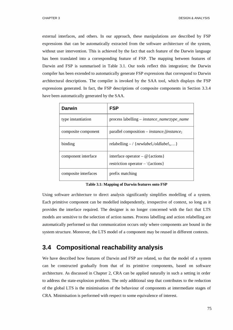
CHAPTER 3 DESIGN & ANALYSIS
75
external interfaces, and others. In our approach, these manipulations are described by FSP
expressions that can be automatically extracted from the software architecture of the system,
without user intervention. This is achieved by the fact that each feature of the Darwin language
has been translated into a corresponding feature of FSP. The mapping between features of
Darwin and FSP is summarised in Table 3.1. Our tools reflect this integration; the Darwin
compiler has been extended to automatically generate FSP expressions that correspond to Darwin
architectural descriptions. The compiler is invoked by the SAA tool, which displays the FSP
expressions generated. In fact, the FSP descriptions of composite components in Section 3.3.4
have been automatically generated by the SAA.
Darwin FSP
type instantiation process labelling –instance_name:type_name
composite component parallel composition –instance1||instance2
binding relabelling – / {newlabel1/oldlabel1,…}
component interface interface operator – @{actions}
restriction operator – \{actions}
composite interfaces prefix matching
Table 3.1: Mapping of Darwin features onto FSP
Using software architecture to direct analysis significantly simplifies modelling of a system.
Each primitive component can be modelled independently, irrespective of context, so long as it
provides the interface required. The designer is no longer concerned with the fact that LTS
models are sensitive to the selection of action names. Process labelling and action relabelling are
automatically performed so that communication occurs only where components are bound in the
system structure. Moreover, the LTS model of a component may be reused in different contexts.
3.4 Compositional reachability analysis
We have described how features of Darwin and FSP are related, so that the model of a system
can be constructed gradually from that of its primitive components, based on software
architecture. As discussed in Chapter 2, CRA can be applied naturally in such a setting in order
to address the state-explosion problem. The only additional step that contributes to the reduction
of the global LTS is the minimisation of the behaviour of components at intermediate stages of
CRA. Minimisation is performed with respect to some equivalence of interest.

CHAPTER 3 DESIGN & ANALYSIS
76
Various notions of equivalence can be used to compare the behaviours represented by two LTSs,
including strong and weak equivalence [Milner 89] and trace and failures-divergence equivalence
[Hoare 85]. In the context of system analysis, an equivalence must be able to distinguish exactly
those features of system behaviour that are relevant to the analysis. The definitions of strong and
weak equivalence are essential for our discussions and are provided here.
3.4.1 Semantic equivalences
For the definition of strong and weak semantic equivalences, we need to introduce the following
notation. We say that an LTSP = ⟨S, A, ∆, q⟩ transitswith actiona∈A into another LTSP´ = ⟨ S,
A, ∆, q ⟩, and denote it as⟨ S, A, ∆, q⟩ →a ⟨ S, A, ∆, q ⟩, if (q, a, q ) ∈ ∆. Intuitively, a
transition changes the initial state of an LTS thus transforming it into an LTS that is identical,
except for the initial state.
Strong semantic equivalenceequates LTSs that have identical behaviour when the occurrence of
all their actions can be observed, including that of the silent actionτ. It is the strongest
equivalence defined between LTSs, and preserves all kinds of behavioural properties. Formally,
let ℘ be the universal set of LTSs. Then strong semantic equivalence “∼” is the union of all
relationsR ⊆⊆⊆⊆ ℘×℘ satisfying that (P, Q) ∈ R implies:
1. αP = αQ;
2. ∀ a ∈ Actτ:
• P →a P´ implies∃ Q , Q →a Q´ and (P , Q ) ∈ R.
• Q →a Q´ implies∃ P , P →a P´ and (P , Q ) ∈ R.
Weak semantic (or observational) equivalenceequates systems that exhibit the same behaviour
to the external observer who cannot realise the occurrence ofτ-actions. Formally, letP⇒a P´
denote '** PP a → ττ , whereτ* means zero or moreτ’s. Then weak semantic equivalence “≈” is
the union of all relationsR ⊆⊆⊆⊆ ℘×℘ satisfying that (P, Q) ∈ R implies:
1. αP = αQ;
2. ∀ a ∈ Act ∪ { ε}, whereε is the empty sequence (soP→ε P):
• P ⇒a P´ implies∃ Q , Q ⇒a Q´ and (P , Q ) ∈ R.
• Q ⇒a Q´ implies∃ P , P ⇒a P´ and (P , Q ) ∈ R.

CHAPTER 3 DESIGN & ANALYSIS
77
Both strong and weak equivalence arecongruenceswith respect to the composition, relabelling,
and hiding operators. This means that strongly or weakly equivalent components may substitute
one another in any system constructed with these operators, without affecting the behaviour of
the system with respect to strong or weak equivalence, respectively.
3.4.2 Reduction of the state space
As discussed in Section 2.6.2, the equivalence notion used for simplifying intermediate systems
in CRA must be strong enough to preserve properties of interest, and weak enough to achieve a
good reduction of the state space. Unlike strong equivalence, observational equivalence is weak
enough to achieve a good reduction of the state space for most systems. Moreover, observational
equivalence captures the notions of encapsulation and interface in a system, inherent in its
software architecture: the environment of a component can only distinguish the behaviour of the
component that is available at its interface. For the above reasons, we have selected observational
equivalence as the default in our CRA approach. Although observational equivalence preserves
safety aspects of a system, it may overlook information necessary for reasoning about liveness,
an issue that is further discussed in Chapter 4.
trans:CHANNELtx:TRANSMITTER
cnt:COUNTER
chnAck:CHANNEL rx:RECEIVER
utx:TRANS_CHNL urx:REC_CHNL
ABP
pr_tx:PR_TX
Figure 3.9: Compositional hierarchy for the ABP protocol
To summarise, our approach computes the model of a system based on its software architecture,
as follows. In Darwin, a system is organised as a hierarchy of components, with primitive
components at the leaves and composite components at the non-leaf nodes of the hierarchy. For
example, Figure 3.9 illustrates the hierarchy defined by the software architecture of the ABP
component of Figure 3.8. The behaviour of primitive components is modelled in terms of LTSs,
specified in FSP. Moreover, an FSP expression for each composite component is automatically
generated from the Darwin description of the software architecture. CRA is then performed
naturally on a system described in this way. The LTSs of composite components are computed in

CHAPTER 3 DESIGN & ANALYSIS
78
stages, as required by CRA. At each intermediate stage, the FSP expression of a composite
component dictates the way in which LTSs of more primitive components are manipulated and
combined for constructing the LTS of its behaviour. Each LTS thus obtained can be analysed
with respect to properties that refer to this component. Subsequently, this LTS is minimised with
respect to observational equivalence, before being used to compute the behaviour of other
components.
We use the two versions of the alternating-bit protocol presented earlier in this chapter to
illustrate how software architecture directs CRA in the generation of system behaviour. In our
evaluation of the reduction achieved with CRA, we use the following terms introduced by [Graf
and Steffen 90] (see also Section 2.6.2):
• apparentcomplexity of a system is the size of its state space before minimisation,
• real complexity of a system is the size of its minimised state space,
• algorithmic complexity of a system is the size of the maximal transition system
encountered by CRA.
3.4.3 CRA of the alternating-bit protocol
Version 1
We first perform CRA on the version of the protocol that allows the transmitter any number of
retransmissions. This version is obtained by using an infinite counter to control these
retransmissions (see Figure 3.5).
Table 3.2 presents the sizes of the LTSs obtained with CRA. For each component type, the LTS
“before minimisation” is the LTS obtained by composing the minimised LTSs of its sub-
components. By minimising this LTS, we obtain the LTS “after minimisation”, which is used by
CRA to compute the LTSs of higher-order components. Additionally, the table displays the sizes
of the LTSs obtained with incremental composition without minimisation. The protocol has an
algorithmic complexity of 468 states and 996 transitions (the largest LTS in the “CRA - before
minimisation” column) and a real complexity of 28 states and 59 transitions (the minimised LTS
for ABP), as compared to an apparent complexity of 4,446 states and 11,646 transitions (ABP
computed without intermediate minimisation).
Note that we have performed incremental composition without minimisation in order to illustrate
how the reduction achieved with CRA becomes gradually more significant for higher-order

CHAPTER 3 DESIGN & ANALYSIS
79
components. However, there is no benefit in computing the LTS of a system gradually if
intermediate LTSs are not minimised. The LTS generated in this way has the same size as the
one obtained by composing the primitive LTSs of the system in a single step; of course, for a
single-step composition, action relabelling must be performed on theflattened software
architecture of the system. Therefore, in order to avoid the risk of intermediate state explosion,
the apparent complexity of a system is typically computed as a single-step composition of its
components. This is also the way we compute it from now on.
CRA
before minimisation after minimisation
Incremental compositionwithout minimisationComponent
#states #trans. #states #trans. #states #trans.
PR_TX 86 132 32 78 86 132
COUNTER 1 2 1 2 1 2
CHANNEL 13 24 7 18 13 24
RECEIVER 36 72 18 54 36 72
TRANSMITTER 28 68 20 60 74 114
TRANS_CHNL 74 198 68 186 302 624
REC_CHNL 66 128 60 156 168 366
ABP 468 996 28 59 4,446 11,646
Table 3.2: State spaces for ABP with infinite retransmissions and channels of capacity one
Analysis: The behaviour of concurrent and distributed systems typically does not terminate, but
consists of continual interaction of the system with its environment. In the LTS models of such
systems, deadlock is easily identified as a state that has no outgoing transitions. Our analysis tool
detected a deadlock in our model of the protocol, and generated a trace in the LTS of the ABP
that may lead to a deadlock. Such traces, which we refer to ascounterexamples, are used to show
an example execution of the system that exhibits erroneous behaviour. They provide invaluable
help for debugging a design. The result obtained is the following:
Trace to DEADLOCK: < accept.1 >
Since analysis is performed compositionally, we have been able to check that all intermediate
subsystems are deadlock-free. The deadlock is therefore introduced when components
utx:TRANS_CHNL and urx:REC_CHNL are combined. The same trace to deadlock is returned for
theABP component without hiding (i.e. when “@{accept, result, deliver} ” is ignored in its
FSP specification). It can therefore be concluded that the deadlock occurs before any interaction
takes place between componentsutx andurx . After accepting a message, the only behaviour that
utx is allowed to perform without interacting withutx is to forward this message to the channel,
timeout and retransmit the message. However, the channel may have committed to transmit the

CHAPTER 3 DESIGN & ANALYSIS
80
message it contains. In this case, it can only accept a retransmission after sending the message to
urx . Similarly, urx finds itself in a state where the receiver is ready to retransmit an
acknowledgement, but the channel is full and waits forutx to be able to receive the
acknowledgement.
The deadlock is therefore caused by the fact that the channels have a capacity of one. Assume
that the model of the channel always offered the choice of losing a message after receiving it.
Then the above deadlock would have been concealed by the fact that the channels would simply
lose their respective messages. This is indeed what happens with the model presented by [Blair,
et al. 98]. In order to detect the deadlock, they resort to checking the protocol again with reliable
channels. The non-deterministic channel that we have specified is therefore, clearly, a better
model of a lossy channel.
Corrected version: In order for the protocol to be deadlock-free, the channels used must have
infinite capacity. As our approach only deals with finite LTSs, we model these as channels that
overwrite messages, as follows:
CHANNEL= ( in[b:BIT][x:VALUES] -> LOSE
| in[b:BIT][x:VALUES] -> TRANSMIT[b][x]),
LOSE = ( lose -> CHANNEL
| in[b:BIT][x:VALUES] -> LOSE
| in[b:BIT][x:VALUES] -> TRANSMIT[b][x]),
TRANSMIT[b:BIT][x:VALUES]=( out[b][x] -> CHANNEL
| in[i:BIT][v:VALUES] -> LOSE
| in[i:BIT][v:VALUES] ->TRANSMIT[i][v]) @{in, out}.
This channel is always ready to receive a new message, and make a new non-deterministic
choice accordingly. Overwriting messages does not introduce a problem in ABP. When the new
message is tagged with the same bitb as the one currently contained in the channel, it is
considered as a retransmission of the same message. When the new message is tagged with bit
!b , it means that the round characterised by bitb has been completed, and messages of that round
will be ignored.
Table 3.3 reports the state spaces of components of ABP when the new model is used for the
channels. Note that CRA needs only re-compute the componentsTRANS_CHNL, REC_CHNLand
ABP, which are affected by the change in the behaviour of the channels. The minimised LTS for
the ABP component is illustrated in Figure 3.10, and clearly shows the correctness of the
protocol. In essence, the protocol behaves as a 1-slot buffer, with the difference that it
additionally reports successful transmission.

CHAPTER 3 DESIGN & ANALYSIS
81
CRAbefore minimisation after minimisationComponent
#states #transitions #states #transitions
CHANNEL 8 103 7 90
TRANS_CHNL 74 246 56 168
REC_CHNL 66 216 48 138
ABP 108 246 7 9
Apparent complexity: 3,906 states and13,560 transitions
Table 3.3: State spaces of ABP with infinite retransmissions and infinite channels
ABP
accept.1
accept.2
accept.3 deliver.3
result.ok.3
deliver.2
result.ok.2
deliver.1
result.ok.1
0 1 2 3 4 5 6
Figure 3.10: LTS for ABP with infinite retransmissions and infinite channels
Version 2
In the second version of the protocol, a bounded counter is used that allows a maximum of two
transmissions of the same message (see Figure 3.5). The channels used are infinite channels, as
introduced in the previous version of the protocol.
CRAbefore minimisation after minimisationComponent
#states #transitions #states #transitions
PR_TX 86 132 32 78
COUNTER 3 6 3 6
CHANNEL 8 103 7 90
RECEIVER 36 72 18 54
TRANSMITTER 64 140 30 82
TRANS_CHNL 96 334 96 334
REC_CHNL 66 216 48 138
ABP 3762 10878 786 2133
Apparent complexity: 35,724 states and116,124 transitions
Table 3.4: State spaces of ABP with bounded retransmissions and infinite channels
CHAPTER 3 DESIGN & ANALYSIS
82
Table 3.4 reports the sizes of the LTSs obtained for the components of the protocol. This version
of the protocol has a real complexity of 786 states and 2,133 transitions and an algorithmic
complexity of 3,762 states and 10,878 transitions, as compared to an apparent complexity of
35,724 states and 116,124 transitions.
Discussion
For both versions of the alternating-bit protocol, compositional minimisation achieves a
reduction of the apparent complexity by at least one order of magnitude in terms of algorithmic
complexity, and by at least two in terms of real complexity. This reduction becomes significant
when the protocol is used as a component of a larger system. The intermediate state machines
obtained do not require the use of contextual interfaces in CRA.
The LTS obtained with CRA for version 1 of ABP is small, and clearly illustrates the correctness
of the protocol (see Figure 3.10). On the other hand, it is impossible to check correctness of
version 2 by simply observing the LTS of its behaviour, since the later contains 786 states and
2,133 transitions. For such cases, one needs to identify properties that guarantee the correctness
of the protocol, and to check the system against these properties. Model checking in the context
of CRA is discussed in Chapters 4 and 5. In Chapter 5, we prove that version 2 of the protocol is
in fact incorrect. It is worth mentioning that the problem is not detected in [Valmari 93b] where
this version of the protocol is described and modelled.
3.5 Related work
Good architectural design is a major factor in determining the success of a software system
[Shaw and Garlan 96]. Analysis can assist in discovering architectural problems early in the
development cycle. Therefore, various existing architectural development environments support
some sort of analysis. For instance, the UniCon environment [Shaw, et al. 95] incorporates the
RMA tool for analysis of real-time properties [Klein, et al. 93]. In UniCon architectural
descriptions, designers can also record real-time characteristics of their systems. These
characteristics are automatically extracted and passed in the appropriate format to the RMA tool,
for analysis of time-dependent properties.
Rapide is an event-based, executable ADL, designed for prototyping system architectures
[Luckham, et al. 95]. Its model of execution distinguishes true concurrency from interleaving: it
is based on partially-ordered sets of events (posets), where events are ordered according to their
time and causal dependencies. Simulating a Rapide architecture generates an execution of the
architecture, as a poset of events. Executions can be illustrated, animated in a graphical, real-time

CHAPTER 3 DESIGN & ANALYSIS
83
environment, and checked against properties. However, for most systems, there are too many
possible executions to be explored with simulation, even at the architecture level. Therefore,
although analysis by simulation can increase confidence in an architecture, it does not perform an
exhaustive check as model checking does.
[Allen and Garlan 97] propose to enrich architecture descriptions in WRIGHT with behavioural
specifications in CSP [Hoare 85]. This permits them to use the FDR analysis tool [Roscoe 94] to
automatically check deadlock freedom for connectors and compatibility of components with the
connectors used. Their work does not currently handle the issue of hierarchical description. A
difference between WRIGHT and Darwin is that Darwin does not have a separate connector
construct: connectors are modelled in exactly the same way as components. For example, the
CHANNELcomponent in our ABP example corresponds to a connector. From the behavioural point
of view, Darwin may simplify the description of a system, due to the fact that connectors do not
need to bealwaysinterposed between components. In this way, connectors can be omitted when
their behaviour is not crucial, in which case the communication primitive of the model is used
instead.
In a WRIGHT architecture description, structural and behavioural specifications are combined.
Therefore, unlike Darwin, WRIGHT does not support a clear separation between the different
views of a system. Moreover, WRIGHT lacks tool support for graphically illustrating
architectures, and for automatically extracting CSP specifications and providing them to the FDR
tool for analysis. In comparison, the integration of our methods and tools is the strongest asset of
our approach. Structural specifications can be provided separately from behavioural ones, but are
exploited directly, and automatically, for system analysis. This includes hierarchical descriptions.
Finally, as described in the following chapters, our approach includes a variety of model-
checking capabilities.
[Naumovich, et al. 97] check the WRIGHT architecture description of a self-serve gas station
system using two existing analysis tools: FLAVERS, based on data-flow analysis [Dwyer and
Clarke 94], and INCA, based on flow equations [Corbett and Avrunin 95]. To perform this, they
manually translate the CSP specifications in the WRIGHT description into Ada code, which is
the input language of both FLAVERS and INCA. In [Magee, et al. 99], we demonstrate that the
gas station system can be checked more elegantly using our approach, due to the efficient
integration of our methods and tools.
Finally, [Inverardi and Wolf 95] describe software architectures using the Chemical Abstract
Machine formalism (or CHAM) [Berry and Boudol 92]. The high level of abstraction and

CHAPTER 3 DESIGN & ANALYSIS
84
conciseness of CHAM descriptions facilitate analysis of software architectures. However, such
analysis is performed manually by the authors. Moreover, the CHAM is not addressed
specifically to software architectures. As pointed out by [Allen and Garlan 97], there are
important methodological reasons for providing specialised notations for architectural
specification. In order to match the architect’s informal design practices, such notations must
provide with explicit constructs for describing architectural abstractions (e.g. components and
configurations).
3.6 Summary
For increased usability, analysis methods and tools should be integrated with other activities of
software development. In TRACTA, software architecture is used to bridge the gap between
design, analysis, and construction of distributed systems. TRACTA uses Darwin to describe
software architecture as a hierarchy of components. Behaviour is modelled in terms of LTSs,
which are described in the FSP specification language. FSP can be viewed as a specialised
language for our framework; it provides a concise way of describing the behaviour of
components in the context of software architecture.
This chapter has shown how system structure can be exploited for analysis. The approach is
based on the fact that each feature of Darwin has been mapped onto a corresponding feature of
FSP. In this way, the structure of any composite component can be automatically translated into
an FSP expression, which describes how its behaviour can be computed from that of its sub-
components. As advocated by CRA, a smaller LTS will be obtained from this procedure by first
minimising the LTSs of the sub-components.
The behaviour of a system can therefore be obtained from that of its primitive components, by
successively computing and minimising the behaviour of its subsystems based on its software
architecture. We have illustrated our discussions with the familiar example of the alternating-bit
protocol. This example highlights the tight integration between design and analysis in our
approach, and indicates the significant reduction that CRA may achieve on the state space of the
system.
85
Model Checking of LTSs 44.1 EXPRESSING PROPERTIES OVER ACTIONS 86
4.2 TEMPORAL LOGIC AND FINITE AUTOMATA 89
4.3 PROGRAM VERIFICATION 95
4.4 SAFETY AND LIVENESS 99
4.5 CHECKING PROPERTIES IN THE CONTEXT OFCRA 101
4.6 OPTIMISATION OF THERD ALGORITHM 107
4.7 DISCUSSION 109
4.8 SUMMARY 110
Model checking consists of constructing a finite-state model of a system and checking this model
against a set of desired properties. As described in Chapter 2, these properties can be expressed
either in some temporal logic (temporal logic approach), or as automata (automata-theoretic
approach). [Vardi and Wolper 86] have proven that temporal logic model checking can be recast
in terms of automata, thus relating these two approaches. Their method is based on translating
LTL formulas into Büchi automata for verification.
A tool may therefore easily provide the choice of expressing properties as automata or as LTL
formulas, since the same checking procedure applies to both. Model checking then consists of the
following basic steps:
1. generate a finite-state model of the system behaviour;
2. express the properties that the system must satisfy in LTL or as Büchi automata;
3. check that the system satisfies its properties;
4. provide counterexamples when the system violates any of its desired properties.
In Chapter 3, we have motivated the use of CRA for creating the LTS corresponding to a system.
This LTS is obtained by successively computing and simplifying the LTSs of its subsystems,
based on the system software architecture. In this chapter, the general mechanisms for model
checking of LTL formulas and Büchi automata are adjusted to our framework, where system
behaviour is described as an LTS that is constructed with CRA.

CHAPTER 4 MODEL CHECKING OF LTSs
86
4.1 Expressing properties over actions
In Section 2.1.1, we described a way of expressing and checking LTL properties of a system
modelled as a Kripke structureK. Such structures are finite-state systems, where states are
labelled with atomic propositions from a setP that hold at these states, and transitions are not
labelled. Atomic propositions inP take the form (ui equalsv), whereui is a state variable of the
system andv is a value forui. A proposition (ui equalsv) is true in all states whereui has valuev.
The properties of the system are then expressed as LTL formulas built from atomic formulas in
P, and are interpreted on the paths of the Kripke structureK.
In contrast, LTS states do not explicitly hold information related to the local values of the state
variables. Rather, each state is characterised by the actions that may be performed when the
system is in this state, and the state transitions that these actions trigger. This is also reflected by
the notions of strong and weak equivalence associated with LTSs. It is therefore natural to
express properties of LTSs in terms ofactions in their alphabets. To this aim, we introduce a
linear temporal logic ofactions (ALTL – Action LTL). ALTL is a restricted version of LTL:
atomic propositions are actions and the interleaving model of concurrency is a built-in feature of
the logic.
4.1.1 ALTL – a linear temporal logic of actions
The syntax of ALTL is similar to the syntax of LTL (see Section 2.1.1), with the difference that
the set of propositions from which formulas are built is the universal set of observable actions
Act (properties are not allowed to refer to the actionτ). In this context, an ALTL interpretationI
is an infinite sequence of assignments of truth-values to the items ofActτ. For some time instant
s∈N and actiona∈Actτ, I(s, a)=true means thata occurs at time instants. In order to enforce the
interleaving model of concurrency in ALTL, two distinct actions are not allowed to be true
(occur) at the same time instant. Formally, an interpretationI is legal iff:
∀ai, aj∈Actτ, I(s, ai)=true ∧ I(s, aj)=true ⇒ ai = aj.
An infinite word infw over A⊆Actτ is an infinite sequence of actions inA. Each infinite word
infw=a0a1a2… defines an ALTL interpretationI as follows:
∀ s∈N, ∀a∈Actτ, I(s, a) = true iff a = as.
In other words, at times∈N, the only action that is true is the action with orders in infw (where
the order of the first action in the sequence is zero). This is illustrated in Figure 4.1, where each

CHAPTER 4 MODEL CHECKING OF LTSs
87
time instants∈N is associated with the action that is true ats in the interpretation defined by
word infw.
0 1 2 3 N
a1a0 a3a2 …
Figure 4.1: Temporal interpretation defined by an infinite sequence of actions
Infinite words can be represented byω-regular expressions.ω-regular expressions extend regular
expressions with the operatorω that expresses infinite repetition. Following the usual
conventions of regular expressions, juxtaposition represents concatenation,∪ represents union,
and∗ denotes finite repetition. For example,a*bcω represents all infinite sequences that initially
contain a finite number ofa actions followed by a single actionb, followed by an infinite number
of c actions.
We can extend the above discussion for the case of finite words. A finite wordfinw over A⊆Actτ
is a finite sequence of actions inA. A finite word finw=a0a1…an is associated with the following
ALTL interpretationI:
∀ s∈N, ∀a∈Actτ, I(s, a) = true iff ( s ≤ n ∧ a = as).
Definition 1 – An infinite word w satisfiesa temporal formulaf, iff f is initially true in the
interpretationI defined byw, that is, iffI(0, f) = true. ■
4.1.2 Introduction of alphabets into ALTL
Properties are usually concerned with a small set of actions and the temporal relationship
between these actions. For example, mutual exclusion is only concerned with the actions of
entering and exiting a critical section. As a consequence, any other action that a system is able to
perform can be ignored when checking this system for mutual exclusion. Moreover, as discussed
later in the chapter, a component may be associated with a local property that must be satisfied in
any context where the component is used. In expressing such properties, designers concentrate on
the occurrence of actions of the component itself, and should not need to consider additional
actions from all the systems where the component may potentially be used.
ALTL provides the flexibility of associating alphabets with formulas to specify which actions are
considered when checking a system against these formulas. The alphabet of a formula thus
allows to abstract irrelevant details when interpreting the formula on some word.

CHAPTER 4 MODEL CHECKING OF LTSs
88
Definition 2 – Let M ⊆ Act be a set of observable actions, andf a formula associated with
alphabetM (denoted asM=αf). For a wordw, we usew M to denote the word obtained by
removing fromw all occurrences of actionsa∉M. Then an infinite wordw satisfies fiff w M
satisfiesf. ■
Example: Assume a concurrent program that uses a binary semaphoresemin order to ensure
mutual exclusion between two processesP1 andP2. For each processPi, let p(s)i andv(s)i denote
the basic operations onsem, enteri and exiti be the actions of entering and exiting a critical
section, andcsi denote that the process is operating in a critical section. In this context, mutual
exclusion can be expressed by the following ALTL formula:
αf = { enter1, exit1, enter2, exit2},
f = □((enter1 ⇒ (¬enter2Uw exit1)) ∧ (enter2 ⇒ (¬enter1Uw exit2))).
The formula is only concerned with the actions of entering and exiting a critical section. It states
that, at any point in time, if a process enters its critical section, then the other process is not
allowed to do the same until the former exits. We use “weak until” (Uw) in this formula, because
mutual exclusion does not require a process eventually exiting after entering its critical section.
Therefore, at some time instantn, (¬enter2Uw exit1) also holds if¬enter2 remains true ever after.
We will show that the following infinite trace of the concurrent program satisfies propertyf:
w = (p(s)1 enter1 cs1 exit1 v(s)1 p(s)2 enter2 cs2 exit2 v(s)2)ω.
According to Definition 2,w satisfiesf iff w´= w αf = (enter1 exit1 enter2 exit2)ω satisfiesf. The
temporal interpretationI defined byw´ is depicted in Figure 4.2. From this figure, and since the
interpretation follows the same pattern for the time instants not illustrated, we can see that∀i∈N,
I(i, f1)=true, wheref1=(enter1 ⇒ (¬enter2Uw exit1)) ∧ (enter2 ⇒ (¬enter1Uw exit2)). Therefore,
□f1 holds at time instant0. But f = □f1, which means thatw satisfies f, and therefore this
particular trace of the program satisfies mutual exclusion.
0 1 2 3 N
exit1enter1 exit2enter2 …
Figure 4.2: Interpretation defined by (enter1 exit1 enter2 exit2)ωωωω
Note that for an infinite wordw, w M may be finite. For example, letw = ab(cde)ω, and f an
ALTL formula whereαf={a, b} and f = □(a⇒◊b). The wordw αf is finite, and defines an
interpretation wherea is true at time0, b is true at time1, and all actions inActτ are false at any

CHAPTER 4 MODEL CHECKING OF LTSs
89
other moment in time. In this interpretation, (a ⇒ ◊b) is true at time0, and trivially true at all
other times becausea is false. Consequently,w satisfies formulaf. On the other hand, formulag,
whereαg={a, b} and g = (□◊a ∧ □◊b) is not satisfied byw.
Note: From now on, when the alphabet of a formula is not explicitly defined, it is implied that it
consists of the actions that appear in the formula.
4.2 Temporal logic and finite automata
In this section, we present a part of the theory of LTL that is of particular interest to this thesis:
the relation between LTL and finite automata. This relation forms the basis of the automata-
theoretic approach to program verification, which has been adopted by several existing methods
and tools [Aggarwal, et al. 90, Alpern and Schneider 89, Gerth, et al. 95, Holzmann 97].
4.2.1 Büchi automata
Büchi automata are finite automata on infinite inputs. The expressive power of this class of
automata is strictly larger than that of LTL. More specifically, any LTL formula can be
algorithmically translated into a Büchi automaton that accepts exactly those infinite words over
its alphabet that satisfy the formula [Vardi and Wolper 86]. In this section, we introduce the
theory of Büchi automata as related to program verification, and as adapted to reflect their use in
the TRACTA approach.
Definition 3 – A Büchi automatonB is a 5-tuple⟨S, A, ∆, q0, F⟩, whereS is a finite set of states,
A=αB∪{ τ} is a set of actions whereαB⊆Act denotes thealphabetof B, ∆ ⊆ S×αB×S is a set of
transitions on observable actions,q0∈S is the initial state, andF⊆S is a set of accepting states.■
In the representation of Büchi automata, accepting states are distinguished by a double circle. For
example, Figure 4.3 depicts a Büchi automatongrant_reqwith accepting state0. Büchi automata
are defined similarly to finite automata on finite words, but their accepting condition is different
in order to deal with infinite inputs.
request
grantedgrant_req 1
granted
0
request
Figure 4.3: Büchi automaton and Büchi process for formula□(request⇒⇒⇒⇒ ◊◊◊◊ granted)

CHAPTER 4 MODEL CHECKING OF LTSs
90
An executionof B=⟨S, A, ∆, q0, F⟩ on an infinite word w=a0a1a2… over αB is an infinite
sequenceσ=q0a0q1a1q2..., where (qi, ai, qi+1)∈∆, ∀i ≥0. An executionσ is acceptingiff it contains
some accepting state ofB an infinite number of times. As Büchi automata may be non-
deterministic, there can be several alternative executions of an automaton on a given infinite
word. An infinite wordw is acceptedby B iff there exists an accepting execution ofB on w.
We will denote asL(B) the languageaccepted byB, which is the set of infinite words overαB
accepted byB. The languages accepted by Büchi automata are usually referred to asω-regular
languages, and they correspond exactly to the languages that can be described byω-regular
expressions [Gribomont and Wolper 89]. Among the most interesting properties ofω-regular
languages is that this class is closed under the operations ofunion, intersection and
complementation. This means that given two Büchi automataB1 andB2 over an alphabetA that
accept languagesL(B1) andL(B2) respectively, it is possible to build Büchi automata that accept
the languagesL(B1)∪L(B2), L(B1)∩L(B2), andAω \ L(B1) [Gribomont and Wolper 89, Sistla, et al.
87].
According to the above discussion, automatongrant_req of Figure 4.3 accepts the language
(request* granted)ω, i.e. all infinite sequences for which requests can only occur finitely often
before one of them is granted. Any other sequence of actions results in an execution of the
automaton that does not contain the accepting state infinitely often. The language ofgrant_req
defines exactly those infinite sequences over {request, granted} that satisfy the ALTL formula
□(request⇒◊granted). This formula states that, at any moment in time, if arequestevent occurs,
then it is eventually followed by agrantedevent.
Emptiness:An automatonB is calledemptyiff L(B) = Ø, i.e. iff it does not accept any word over
its alphabet. A Büchi automaton is non-empty iff at least one cycle in its graph contains some
accepting state [Gribomont and Wolper 89]. This can be explained intuitively as follows. For
finite-state systems, an infinite execution can be obtained by following a path to some stater of
some cycle, and then indefinitely following the path fromr to r defined by the cycle. If the cycle
contains some accepting state, then the execution is accepting.
4.2.2 The role of alphabets
Traditionally, the language of a Büchi automaton does not contain words that are not over its
alphabet [Gribomont and Wolper 89]. However, in TRACTA, the alphabet of a Büchi automaton
plays the same role as the alphabet of an ALTL formula; it expresses which actions in an infinite

CHAPTER 4 MODEL CHECKING OF LTSs
91
word must be checked by the automaton, in order to decide if the word is accepted or not. All
remaining actions are of no relevance to the property that the automaton expresses, and therefore
their occurrence is ignored. This is achieved by a simple extension that we have made to the
definition of an “execution” of a Büchi automaton (the definition of an “accepting execution”
remains the same):
Definition 4 – An execution of a Büchi automatonB = ⟨S, A, ∆, q0, F⟩ on an infinite word
w=a0a1a2…overA1⊇αB is an infinite sequenceσ = q0a0q1a1q2..., where:
∀ i ≥ 0, ((qi, ai, qi+1) ∈ ∆ if ai∈αB) and (qi = qi+1 if ai∉αB). ■
A Büchi automatonB with alphabetαB accepts an infinite wordw iff there exists a traditional
execution of the automaton onw αB that: – is accepting whenw αB is infinite, or – leaves the
automaton in an accepting state whenw αB is finite. The extension described in Definition 4
covers exactly these cases. Büchi automata can thus perform similar abstractions as ALTL
formulas do. In general, an ALTL formulaf may be algorithmically translated into a Büchi
automaton with the same alphabet, which accepts those infinite words overActτ that satisfyf. The
automaton forf is the result of translatingf, viewed as an LTL formula, into a traditional Büchi
automaton with alphabetαf. The construction of the Büchi automaton must take into account that
at most one action can be true at any time instant.
a
bB 1
b
0
a
Figure 4.4: A Büchi automaton representing formulaf = □(a ⇒⇒⇒⇒ ◊◊◊◊b)
For example, consider an infinite wordw = ab(cde)ω, and an ALTL formulaf=□(a⇒◊b) with
αf={a, b}. In Section 4.1.2, we showed thatw satisfiesf. The same result is obtained by using the
Büchi automatonB corresponding tof, which is illustrated in Figure 4.4. According to Definition
4, the execution ofB on w is σ=0a1b0(c0d0e0)ω; the actionsc, d, e that occur infinitely often in
w do not belong to the alphabet ofB and therefore leave the automaton in state0. As accepting
state0 is contained inσ infinitely often, B accepts the wordw.
Emptiness:Definition 4 allows Büchi automata to accept words that may contain actions outside
their alphabets. We then say that an automatonB is emptyiff it does not accept any word overits
own alphabet, i.e. iffL(B)∩αBω = Ø. Again, a Büchi automaton is non-empty iff at least one
cycle in its graph contains some accepting state.

CHAPTER 4 MODEL CHECKING OF LTSs
92
4.2.3 Büchi processes
As discussed, LTS states do not explicitly hold information related to the local values of the state
variables. Rather, each state is characterised by the actions that may be performed when the
system is in this state, and the state transitions that these actions trigger. Following the principle
of the LTS model, our work introduces a new type of automata called Büchi processes, which are
similar to Büchi automata, but where accepting states are distinguished in terms of transitions
that may be triggered at these states.
Definition 5 – A Büchi processB is a 5-tuple⟨S, A, ∆, q0, L⟩, whereS is a finite set of states,
A=αB∪{ τ} is a set of actions whereαB⊆Act denotes thealphabetof B, ∆ ⊆ S×αB×S is a set of
transitions on observable actions,q0∈S is the initial state, andL⊆αB is a set ofaccepting actions
(such actions are prefixed with the special symbol “@”). The transition relation∆ is such that:
∀ (s, a, t)∈ ∆: a∈L ⇒ (s = t).
In other words, transitions labelled with accepting actions (calledaccepting transitions) can
relate a state only to itself.■
Executions of Büchi processes are defined as for Büchi automata (Definition 4). A Büchi process
B = ⟨S, A, ∆, q0, L⟩ acceptsan infinite wordw, iff there exists an executionσ of B on w such that
all accepting actionsl i∈L are enabled infinitely often inσ. An actiona is enabledin executionσ
iff σ contains a states wherea is enabled. An actiona is enabledat a states∈S, iff ∃s ∈S such
that (s, a, s ) ∈ ∆.
Note that in our approach, actions prefixed with the symbol “@” are reserved for use as
accepting actions; they donot appear in infinite words or in LTSs. Therefore, words that belong
to the language of a Büchi process donot contain accepting actions.
01 2choose2
do2do1
choose1
fair@B
1@B
2
Figure 4.5: A Büchi process modelling fair choice between two alternatives
For example, Figure 4.5 illustrates a Büchi process that models a fair selection between action
do1and actiondo2. Its set of accepting labelsL is equal to {@B1, @B2}. The processfair accepts
only infinite words that contain bothchoose1andchoose2an infinite number of times. This is
because@B1 and@B2 are enabled only at states1 and2 respectively, and therefore an accepting
execution of the automaton must contain both states1 and2 infinitely often.

CHAPTER 4 MODEL CHECKING OF LTSs
93
Emptiness: A Büchi processB is emptyiff it does not accept any words overits own alphabet,
i.e. iff L(B)∩αBω = Ø. Given the accepting condition of Büchi processes, a Büchi process is non-
empty iff all acceptingactions in its alphabet are enabled in at least one cycle of its graph (an
action a is enabled in a cycle iff the cycle contains a state wherea is enabled). Of course,
transitions on accepting actions are not considered when searching for cycles in the graph of a
Büchi processB. As mentioned, such transitions simply mark accepting states, and do not appear
in executions ofB.
Relationship with Büchi automata
Any Büchi automaton can be translated automatically into a Büchi process that accepts the same
words overActτ, as follows:
Definition 6 – A Büchi automatonB = ⟨S, A, ∆, q0, F⟩ is mapped to a Büchi processB´=
⟨S,A∪{ @B}, ∆ , q0, {@B} ⟩ by adding a new globally unique accepting action@B and new
accepting transitions, such that:
• @B∉ A; and
• ∆´ = ∆ ∪ { s → B@ s | s ∈ F}. ■
A Büchi automaton is translated into an equivalent Büchi process by marking its accepting states
with accepting transitions. These transitions are all labelled with the same action “@name”, where
“ name” is the unique identifier of the Büchi automaton. For example, the Büchi automaton
grant_reqof Figure 4.6 is transformed into the Büchi processgrant_req in the same figure.
request
granted
grant_req 1
granted
0
request
request
grantedgrant_req 1
@grant_reqgranted
0
request
Figure 4.6: Transformation of a Büchi automaton into a Büchi process
Note that not every Büchi process can be viewed as a direct translation of some Büchi
automaton. That is, we could not use the inverse procedure from that described in Definition 6 in
order to map any Büchi process into an equivalent Büchi automaton. The reason is that for some
Büchi process⟨S, A, ∆, q0, L⟩, L may contain more than one accepting actions (see Figure 4.5). In
fact, Büchi processes directly correspond to a generalised form of Büchi automata, which has the
same expressive power as standard Büchi automata, but allows more concise definitions
[Gribomont and Wolper 89]. The benefit from allowing multiple accepting actions in a Büchi
process is apparent when such processes are composed, as described below.

CHAPTER 4 MODEL CHECKING OF LTSs
94
Composition of Büchi processes
In the following, we define a parallel composition operator for Büchi processes, which is based
on the corresponding operator on LTSs.
Definition 7 (Parallel Composition) – Consider two Büchi processesB1 = ⟨S1, A1, ∆1, q1, L1⟩ and
B2 = ⟨S2, A2, ∆2, q2, L2⟩, and the LTSsP1 andP2 obtained from the first four components of each,
i.e. P1 = ⟨S1, A1, ∆1, q1⟩, andP2 = ⟨S2, A2, ∆2, q2⟩, respectively. The parallel compositionB1||B2 of
B1 andB2 is the Büchi processB = ⟨S, A, ∆, q, L⟩, where⟨S, A, ∆, q⟩ = P1 ||P2, andL = L1 ∪ L2. ■
From Definition 7, it is clear that during their joint execution, Büchi processes do not proceed in
lock-step synchronisation, which is the standard way in which Büchi automata are composed
[Gribomont and Wolper 89]. This is due partly to the fact that Büchi processes are allowed to
have different alphabets, and partly to the extended notion of an execution that our approach has
introduced (see Definition 4).
The theorem that follows forms the basis of the ALTL verification procedure, and is based on a
similar theorem for Büchi automata (Theorem 4.4 in [Gribomont and Wolper 89]). However, our
theorem applies to Büchi processes, and therefore takes into account the particular way in which
Büchi processes are composed.
Theorem 4.1– The parallel composition of two Büchi processes accepts the intersection of their
languages. That is, for any two Büchi processesB1 andB2, the following holds:
B = B1||B2 ⇒ L(B) = L (B1) ∩ L(B2).
Proof. Let B1 = ⟨S1, A1, ∆1, q1, L1⟩ and B2 = ⟨S2, A2, ∆2, q2, L2⟩ be two Büchi processes and
B=B1||B2. Assume thatB = ⟨S, A, ∆, q, L⟩. Then, from Definition 7, we know thatL = L1 ∪ L2,
and⟨S, A, ∆, q⟩ = ⟨S1, A1, ∆1, q1⟩ || ⟨S2, A2, ∆2, q2⟩. Therefore, the states ofB can be represented as
pairs of states ofB1 and B2. From Definition 5, a wordw belongs toL(B) if there exists an
executionσ of B on w which contains infinitely often, for each accepting actionl i in L1∪L2, a
state wherel i is enabled. From the semantics of the composition operator and Definition 4, the
projectionσ1 of executionσ on the states ofB1 coincides with an execution ofB1 on w. Since for
eachl i∈ L1, l i is enabled inσ, σ1 is an accepting execution ofB1 on w. This means thatw ∈ L(B1).
Similarly, w ∈ L(B2), and thereforew∈(L(B1)∩L(B2)). We have thus proven thatw∈L(B) ⇒
w∈(L(B1)∩L(B2)).
To prove the inverse, assume thatw∈(L(B1)∩L(B2)), and thatw=a0a1a2.... Then, there exists an
accepting executionσ1 of B1 on w, and an accepting executionσ2 of B2 on w. Let σ1 =

CHAPTER 4 MODEL CHECKING OF LTSs
95
r0a0r1a1r2... andσ2 = s0a0s1a1s2… We argue that executionσ = (r0, s0) a0 (r1, s1) a1 (r2, s2)… is a
possible execution ofB1||B2 on w. We prove this by showing that∀i≥0, (r i, si) ai (r i+1, si+1) is a
legal step ofB1||B2, when executing onw. Let us callti the transition ((r i, si), ai, (r i+1, si+1)). In the
case where actionai∈ (αB1∩αB2), and given thatσ1 andσ2 are executions ofB1 andB2 on word
w, (r i, ai, r i+1) is a transition ofB1, and (si, ai ,si+1) is a transition ofB2. Therefore,ti is a transition
of B1||B2, and, by Definition 4,(r i, si) ai (r i+1, si+1) is a legal step in an execution ofB1||B2 on w.
Whenai∈ (αB1–αB2), (r i, ai ,r i+1) is a transition ofB1, whereassi = si+1. So,ti is again a transition
of B1||B2. We argue similarly for the case whereai∈ (αB2–αB1). Finally, whenai∉(αB1∪αB2), r i
=r i+1 and si=si+1. Moreover, according to Definition 4,B1||B2 does not change state when
executing on actionai, which proves that(r i, si) ai (r i+1, si+1) is a legal step in an execution of
B1||B2 on w. We can therefore conclude thatσ is a possible execution ofB1||B2 on w. It is easy to
prove that, in addition,σ is an accepting execution. The projection ofσ on states ofB1 andB2 is
identical toσ1 andσ2, respectively. Sinceσ1 andσ2 are accepting executions ofB1 andB2, andL
= L1∪L2, each accepting actionl i∈L is enabled infinitely often inσ, which makesσ an accepting
execution. We conclude thatw∈(L(B1)∩L(B2)) ⇒ w∈L(B), which completes the proof.■
4.3 Program verification
When a program is executed on a computer, a sequence of machine states is generated. This
sequence, enriched with the program statements whose execution causes the transition of each
state to the next, is called an execution. If program statements are mapped to actions, then the
sequence of statements in a program execution defines a word, which may be checked against
ALTL properties. Concurrent programs usually admit several executions due to the fact that, at a
given state, more than one statement may be selected for execution. Obviously enough, such
programs are correct with respect to some ALTL property iffall their possible executions satisfy
this property. For a program modelled as an LTS, this is formally described as follows:
An LTS satisfiessome ALTL formulaf, iff all its possible executions satisfyf. An
executionof an LTSP = ⟨S, A, ∆, q0⟩ is an infinite sequenceσ = q0a0q1a1q2..., where:
∀ i ≥ 0, (qi, ai, qi+1) ∈ ∆. An executionσ = q0a0q1a1q2... satisfiesf, iff its corresponding
infinite word w=a0a1a2... satisfiesf.
Intuitively, properties expressed in ALTL are interpreted and checked on the infinite sequences
of actions that an LTS can perform. To simplify our discussion, we assume that LTSs do not
contain transitions on the actionτ. Later in this section, we show that the verification procedure
that we present can also be applied to LTSs that contain such transitions.

CHAPTER 4 MODEL CHECKING OF LTSs
96
4.3.1 Procedure
Let PLTS= ⟨S, A, ∆, q⟩ be the LTS model of a concurrent system, which does not containτ-
transitions. This LTS can be viewed as Büchi automatonP= ⟨S, A, ∆, q, S⟩ which, among the
infinite words overαP, accepts exactly those that correspond to executions ofPLTS [Gribomont
and Wolper 89]. Formally,
L(P)∩αPω= { w∈αPω | w corresponds to some infinite execution ofPLTS}.
Let P´ be the Büchi process for this automaton (that is,L(P´)= L(P)). To check thatPLTS satisfies
some ALTL propertyf, we proceed as follows:
Step 1. Build a Büchi processB¬f = ⟨S1, A1, ∆1, q1, {@B} ⟩ for ¬f.
Comment: In general, it is more efficient to build a Büchi automaton for the negation of a
formula, than to build and then compute the complement of the automaton for the formula itself.
Complementation of Büchi automata is an expensive operation [Gribomont and Wolper 89],
whereas there exist efficient algorithms for constructing an automaton corresponding to some
LTL formula [Gerth, et al. 95]. The same holds for Büchi processes and ALTL formulas.
Step 2. Compute the Büchi processI = P´||B¬f.
Comment: Let W be the set of infinite words overαI accepted byI, i.e. W=L(I)∩αIω. By
Theorem 4.1,αI=αP´∪αB¬f, and sinceαP´=αP∪{@P}, it holds that αI=αP∪{@P} ∪αB¬f.
However, formula¬f expresses an (undesired) property ofPLTS, soα(¬f) ⊆ αPLTS=αP. We also
know thatαB¬f =α(¬f)∪{@B}. Therefore,αI = αP∪α(¬f)∪{@P, @αB} = αP∪{@P, @αB}.
But since words inL(I) cannot contain accepting actions, we conclude thatW=L(I)∩αPω.
By Theorem 4.1,L(I) = L(P )∩L(B¬f) = L(P)∩L(B¬f), and soW=L(P)∩L(B¬f)∩αPω. This means
that the set of infinite words thatI accepts over its own alphabet contains exactly the executions
of PLTS (L(P)∩αPω) that are accepted byB¬f , i.e. that satisfy¬f.
Step 3. Check thatI is empty.
Comment: This means that there exists no execution ofPLTS that satisfies¬f, i.e. PLTS satisfiesf.
The set of accepting actions of Büchi processI is equal to {@P} ∪{@B}={@ B, @P}. So process
I accepts a wordw iff there exists an execution ofI on w where both @B and @P are enabled
infinitely often. But @P is enabled at all states ofP , so it is also enabled at all states ofI.
Therefore, since condition @P is trivially satisfied, the set of accepting actions ofI can be

CHAPTER 4 MODEL CHECKING OF LTSs
97
reduced to {@B}. We conclude that the LTS of a concurrent program can be used directly for
verification; it is not necessary to add accepting transitions to it.
Checking emptiness:Step 3 in the above procedure requires checking if the Büchi processI is
empty. I is non-empty iff @B is enabled in at least one cycle of its graph. This is known to
reduce to checking that there exists anon-transientstrongly-connected component inI (see
Definition 8) where @B is enabled [Gribomont and Wolper 89]. The latter can be performed with
time complexity linear in the size of the graph [Tarjan 72].
Definition 8 – A strongly-connected component is a maximal set of states such that every state in
the set is reachable from any other state in the set. Atransientstrongly-connected component has
only one state and there is no transition from that state to itself other than accepting transitions,
which are prefixed with the special symbol @. Any other strongly-connected component is called
non-transient. ■
Note that accepting transitions are ignored when deciding if a strongly-connected component is
transient, since they are simply used to distinguish accepting states. For example, the graph of
Figure 4.8 contains the following strongly-connected components: {0,5,6} and {2,3,4} which are
non-transient, and {1} which is transient.
Counterexamples:Assume that step 3 of the model-checking procedure detects a violation, i.e.
@B is enabled in some strongly-connected componentSCCof processI. A counterexample can
then be provided to help uncover the error in the design. A counterexample describes an infinite
word corresponding to some violating execution ofPLTS. In TRACTA, such counterexamples are
of the formseq1(seq2)ω, where:
• seq1 is a trace ofI to some stater of SCCwhere @B is enabled, and
• seq2 is a trace from stater, corresponding to a cyclic path inI. Note that action @B does
not occur inseq2.
Terminating executions:Our approach is focused on concurrent and distributed systems, where
terminating executions are typically considered as deadlocks. However, verification with Büchi
automata can also cover cases where terminating executions are legal. A common practice is to
turn terminating executions into infinite ones by adding a transition labelled with a “terminate”
action from each terminating state to itself.
Unobservable actions:In the above discussion, we assumed, for simplicity, that the LTSs that
we check do not containτ-transitions. Now letP be an LTS that contains noτ-transitions,A be a

CHAPTER 4 MODEL CHECKING OF LTSs
98
set of actions inαP that must be hidden,P´ be the result of hiding actions inA from P, andB be
a Büchi process used for checkingP against some property, such thatαB∩A = Ø. From the
semantics of the parallel composition operator, it is clear that the graphs corresponding toP´||B
andP||B have a single difference: all transitions on actions that belong toA in P||B, are transitions
on the actionτ in P´||B. However, the structure of the two graphs is identical, and therefore,P´||B
is empty iff P||B is empty. In other words, the verification procedure that we have described can
also be applied to LTSs that containτ-transitions. Such LTSs are checked against properties that
are only concerned with their observable actions.
Similarly, Büchi processes can be extended to allowτ-transitions. This often facilitates
modelling, as it allows a Büchi process to perform an internal, non-deterministic, change of state.
For instance, we use such a Büchi process in one of our examples of Chapter 6 (see Figure 6.8).
Note that, sinceτ-actions are considered unobservable in TRACTA, they do not explicitly appear
in counterexamples. However, their existence is implied when it plays a role in a violation. For
example, in a counterexample of the formseq1(seq2)ω, if seq2 contains no actions, then it
obviously describes aτ-cycle in the system behaviour.
4.3.2 Example
Consider version 1 of the alternating-bit protocol presented in Chapter 3. We restrict the values
that the protocol transmits to a single value in order to be able to illustrate graphically the
verification process with Büchi automata. The minimised LTS ofABP is illustrated in Figure 4.7.
We wish to check propertyf = □(accept.1 ⇒ ◊ deliver.1), which states that it is always the case
that if a message is accepted, it is eventually delivered. We proceed according to the model-
checking procedure described earlier in this section:
1. We build a Büchi processL1 corresponding to¬f = ◊(accept.1 ∧ □¬deliver.1), illustrated in
Figure 4.7.
2. We construct the Büchi processABP||L1 . The result is illustrated in Figure 4.8.
3. We check thatABP||L1 is empty. Figure 4.8 clearly shows that this is the case, since@L1is
not enabled in any non-transient strongly-connected component of the graph. We therefore
conclude thatABPsatisfies the property. Given the LTS ofABP, this result was expected.

CHAPTER 4 MODEL CHECKING OF LTSs
99
The automata-theoretic approach thus reduces model checking to a reachability problem,
although in theproductof the state spaces of the system and the property. For example, the LTS
corresponding toABP||L1 has 7 states, as compared to 3 states of the LTS forABP.
ABPaccept.1 deliver.1
result.ok.1
0 1 2L1
accept.1
accept.1
deliver.1accept.1
deliver.1
@L1accept.1deliver.1
0 1 2
Figure 4.7: Minimised ABP protocol, and Büchi process for◊◊◊◊(accept.1 ∧∧∧∧ □¬¬¬¬ deliver.1)
accept.1
accept.1 deliver.1
@L1
result.ok.1 accept.1
deliver.1
deliver.1
result.ok.1
0 1 2 3 4 5 6
Figure 4.8: Composite LTS of ABP with property L1
4.4 Safety and liveness
Various classifications of program properties appear in the literature, where each class is usually
characterised by a canonical temporal formula scheme [Lamport 94, Manna and Pnueli 92]. In
our work, we consider two popular classes of properties, safety and liveness, also referred to as
invariance and eventuality [Lamport 94].
Informally, asafetyproperty claims that “something bad” does not happen. For example, mutual
exclusion is a safety property that specifies the absence of a program state where a common
resource is simultaneously accessed by more than one client. Alivenessproperty claims that
“something good” eventually happens, i.e. that a program eventually enters a desirable state. For
example, the assertion that a program eventually closes a file after opening it is a liveness
property. Safety and liveness properties can also be characterised more formally as follows
[Manna and Pnueli 92]:

CHAPTER 4 MODEL CHECKING OF LTSs
100
• f is a safety property iff any sequence of actions violatingf contains a finite prefix, such
that all infinite extensions of this prefix violatef.
• f is a liveness property iff any arbitrary finite sequence of actions can be extended to an
infinite sequence satisfyingf.
Therefore, when a bad situation occurs at some point in an execution, there is no meaning in
exploring the execution any further. On the other hand, an execution of a program may at any
moment evolve in such a way as to satisfy a liveness property. So we can never judge, by any
finite prefix of the execution, if the liveness property is violated or not. [Alpern and Schneider
87] have shown that any property modelled as a Büchi automaton can be decomposed into a
safety and a liveness property whose conjunction is the original.
Safety properties usually claim that some propertyf holds at every program state. Thus, they take
the form□f, where the truth-value off at any states depends solely on the values of the state
variables ats. The following are some examples of safety properties [Lamport 94]:
• deadlock freedom: f asserts that the program is not deadlocked.
• mutual exclusion: f asserts that at most one process is in its critical section.
Assume that properties for a system can be expressed as state formulas. Then mutual exclusion
between two processes could be expressed as□(¬in_CS1 ∨ ¬in_CS2), wherein_CSi denotes that
the processi is in its critical section. As discussed, LTS states do not explicitly hold information
related to the local value of state variables. Properties are therefore expressed in terms of
sequences of actions. In such a setting, a safety property expresses the fact that subsequent to
specific scenarios, the occurrence of some actions must be prevented if undesirable states in the
system are to be avoided. The example of Section 4.1.2 shows how mutual exclusion can be
expressed in terms of actions.
The following are typical examples of liveness properties [Lamport 94]:
• service: if a process requests a service, it is eventually served:request⇒ ◊serve.
• message delivery: a message sent often enough is eventually delivered, where often
enough is translated as infinitely often: (□◊send)⇒ ◊deliver.
If the service and message delivery properties must hold at any point in a program execution,
then their formulas must be prefixed with□. In the LTS model, liveness properties enforce the
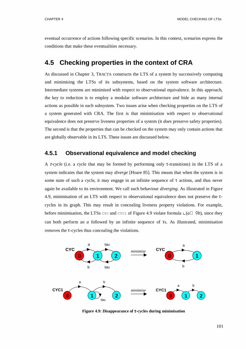
CHAPTER 4 MODEL CHECKING OF LTSs
101
eventual occurrence of actions following specific scenarios. In this context, scenarios express the
conditions that make these eventualities necessary.
4.5 Checking properties in the context of CRA
As discussed in Chapter 3, TRACTA constructs the LTS of a system by successively computing
and minimising the LTSs of its subsystems, based on the system software architecture.
Intermediate systems are minimised with respect to observational equivalence. In this approach,
the key to reduction is to employ a modular software architecture and hide as many internal
actions as possible in each subsystem. Two issues arise when checking properties on the LTS of
a system generated with CRA. The first is that minimisation with respect to observational
equivalence does not preserve liveness properties of a system (itdoespreserve safety properties).
The second is that the properties that can be checked on the system may only contain actions that
are globally observable in its LTS. These issues are discussed below.
4.5.1 Observational equivalence and model checking
A τ-cycle (i.e. a cycle that may be formed by performing onlyτ-transitions) in the LTS of a
system indicates that the system maydiverge[Hoare 85]. This means that when the system is in
some state of such a cycle, it may engage in an infinite sequence ofτ actions, and thus never
again be available to its environment. We call such behaviourdiverging. As illustrated in Figure
4.9, minimisation of an LTS with respect to observational equivalence does not preserve theτ-
cycles in its graph. This may result in concealing liveness property violations. For example,
before minimisation, the LTSsCYCandCYC1of Figure 4.9 violate formula□(a⇒ ◊b), since they
can both perform ana followed by an infinite sequence ofτs. As illustrated, minimisation
removes theτ-cycles thus concealing the violations.
CYCa tau
b tau
0 1 2minimise CYC
a
b
0 1
CYC1
a
tau
b
0 1 2minimise CYC1
a b
0 1 2
Figure 4.9: Disappearance ofττττ-cycles during minimisation

CHAPTER 4 MODEL CHECKING OF LTSs
102
In order to preserve liveness property violations, we propose a modification to the CRA
procedure. This consists of transforming each intermediate LTS before minimising it as
described by the RD algorithm of Figure 4.10. The RD algorithm computes theτ-strongly-
connected componentsof an LTS; these are the non-transient strongly-connected components in
the projection of the LTS on itsτ relation. The strongly-connected components of a graph may be
computed with time complexity linear in the size of the graph [Tarjan 72].
RD Algorithm (Recording Divergence):
Let P= ⟨S, A, ∆, q⟩ be the LTS obtained at some step of CRA, and∆´ be the projection of∆ on
theτ relation. Then:
for directed graph G = <S, ∆’> do // G does not need to be connected
compute the set SCCs of non-transient strongly-connected components;
for every strongly-connected component C with root r in SCCs do {
if (no action prefixed with ~ is enabled at any state of C in ∆)
add ((r, ~P, r) to ∆ in P; // divergence transition
}
Figure 4.10: An algorithm that records divergence
In an LTS, all states of aτ-strongly-connected componentC are observationally equivalent to
each other since, when in some state inC, the LTS can transit into any other state ofC by
performing onlyτ-actions. As a result, the states ofC are mapped to a single state in the
minimised LTS. In order to preserve the diverging behaviour of the system at these states after
minimisation, the RD algorithm adds a specialdivergencetransition to the root ofC (i.e. the first
state ofC encountered by the algorithm during graph exploration). Divergence transitions are
“looping”, i.e. they connect a state to itself, and they are labelled withdivergenceactions named
as “~pr_name ”. The prefix “~” identifies divergence actions from simple actions in an LTS, and
“ pr_name ” is the identifier of the LTS where such transitions are added by the RD algorithm. For
example, the processesCYC and CYC1 of Figure 4.9 are transformed with the RD algorithm as
illustrated in Figure 4.11. The information that systemsCYCandCYC1 may diverge at state1 is
no longer lost after minimisation.
CYC
a
b
~CYC0 1CYC1
a b
~CYC10 1 2
Figure 4.11: LTSs with divergence recorded

CHAPTER 4 MODEL CHECKING OF LTSs
103
Divergence actions are never hidden during CRA. Moreover, the naming of these actions
guarantees that they never synchronise. In this way, all divergence transitions survive across
levels of a compositional hierarchy, unless the states where they are enabled become
unreachable. Therefore, a state in an LTS does not need to contain more than one divergence
transition. For this reason, the algorithm doesnot add diverging transitions to the root of aτ-
strongly-connected componentC when some diverging action is already enabled at some state of
C. That reflects the fact that, in selecting among divergence transitions that apply to the same
state, the RD algorithm shows preference to the one that corresponds to a more primitive
component in the compositional hierarchy.
Assume that, when CRA completes, a diverging action ~pr_name is enabled at some state of the
global LTS of the system. This means that the system may diverge at this state, because its
subsystem “pr_name ” may engage in an infinite sequence ofτ-actions.
Example: In the example of Section 4.3, Büchi automata were used to check that a simplified
version of the ABP protocol satisfies liveness propertyf = □(accept.1⇒ ◊deliver.1). The
simplification refers to the fact that a single value can be transmitted by the protocol. In the
current example, we check the propertyf in a similar way. However, the LTS of the ABP
protocol is generated with the modified CRA procedure, which applies the RD algorithm to every
intermediate system before minimisation. The LTS thus constructed violates propertyf. The
counterexample obtained from our tools represents the following infinite trace:
accept.1(~TRANS_CHNL) ω. This counterexample indicates that component typeTRANS_CHNLmay
diverge after the protocol performs actionaccept.1 .
trans:CHANNELtx:TRANSMITTER
accept
utx:TRANS_CHNL
resres
acceptsend
ack
ack
in
out
send
Figure 4.12: Structure of component TRANS_CHNL of the ABP protocol
Figure 4.12 illustrates the structure of componentTRANS_CHNL(the entire structure of the
protocol is illustrated in Figure 3.8). From the counterexample obtained, we know that
TRANS_CHNLmay diverge after performingaccept.1 . This is not due to divergence in its sub-
components otherwise the RD algorithm would have recorded this fact; as mentioned, the

CHAPTER 4 MODEL CHECKING OF LTSs
104
algorithm shows preference to divergences of more primitive components. Divergence is
therefore introduced whentx:TRANSMITTER and trans:CHANNEL are combined, and actions that
model interaction between these components are hidden (see Figure 4.12). This interaction takes
place between portalsend of tx:TRANSMITTER and portalin of trans:CHANNEL .
Divergence thus occurs when the transmitter keeps sending messages to the channel, without
receiving any acknowledgement from the receiver (we know that divergence occurs before the
receipt of acknowledgements, because theack actions are observable inTRANS_CHNL). This
happens when the transmitter re-transmits a message, times out, and keeps executing these two
actions, without checking if an acknowledgement is waiting to be received. It is easy to detect
thatREC_CHNLdiverges in a similar way.
This example also shows that software architecture may significantly assist in understanding
counterexamples and effectively using them to find the sources of problems in the design.
4.5.2 Reasoning about hidden actions
Although CRA techniques may significantly reduce the system state space, the LTS generated
can only be utilised to validate behavioural properties involving actions that are globally
observable [Cheung, et al. 97, Cheung and Kramer 96a, Giannakopoulou, et al. 99a]. However,
as described below, the desired properties of a system may sometimes involve internal actions of
its subsystems.
A complex system typically contains several subsystems that may be independently developed or
extracted from software libraries. Each of them often assumes a set of predefined communicating
protocols at its interface. These protocols express conditions for the correct use of the
component. For a subsystem to function properly, its protocols must be respected by its
environment. These protocols can therefore be conceived as local safety properties that have to
be satisfied in the composite system.
Similarly, it may be useful to express local liveness properties of subsystems, which must be
respected by the subsystem’s environment. One such case is where one needs to identify if some
component of a system is deadlocked in the context of the system. Assume that a system does not
deadlock, nor do its components when analysed individually. Still, in the system, any one of
these components may, after a certain point, no longer participate in the system behaviour. This
may reflect the failure of this component, as modelled by the developer. In other cases however,
this situation may indicate some synchronisation problem in the design. Another case is where

CHAPTER 4 MODEL CHECKING OF LTSs
105
the usefulness of a component in a system relies on the fact that some basic local liveness
properties of the component are preserved in the context of the system.
Such local properties of components may involve actions that are not globally observable.
Checking them may therefore lead to a need of exposing these actions at the global level of a
system. This contradicts the key philosophy of CRA techniques, and limits their effectiveness in
avoiding state explosion. As the reduction achieved by CRA becomes less significant, the extra
cost incurred by minimisation of intermediate subsystems is no longer justifiable. In TRACTA,
this would additionally introduce changes to component interfaces, thus undermining the tight
integration of analysis with design.
Proposed solution
The objective is to retain the freedom of abstracting (sub-)system behaviour at the various levels
of the system hierarchy, without compromising the effectiveness of analysis. TRACTA achieves
this as follows. When a Büchi process expresses a local property of some subsystem, it is added
in the compositional hierarchy as a component of this subsystem. In this way, the Büchi process
may observe internal actions of the subsystem, even though these actions are not globally
observable. More specifically, assume that a propertyf refers to some subsystemP of systemS,
and contains actions that are not observable inS. Then TRACTA performs analysis as follows:
1. A Büchi processB is constructed for¬f.
2. B is included in the compositional hierarchy ofS as a component ofP. As a resultB
participates in the behaviour ofP and makes it able to record violations of its local propertyf
in any context. Alternatively, ifB contains actions at the interface ofP only, it can be
included in the hierarchy to be composed withP.
3. CRA, enhanced with the RD algorithm, is performed based on the new compositional
hierarchy of the system. Note that the RD algorithm can also be applied to a Büchi process.
Accepting and divergence actions are not hidden during CRA.
4. If the global Büchi process thus obtained contains a non-transient strongly-connected
component where @B is enabled, then the propertyf is violated.
Proof of correctness
With the new mechanism, intermediate systems in CRA can be viewed as Büchi processes, since
one of their sub-components may be a Büchi process. To prove the correctness of our approach,

CHAPTER 4 MODEL CHECKING OF LTSs
106
we show that a Büchi process preserves its violations when transformed as required by CRA. Let
S be the Büchi process for some intermediate system, where@B belongs to the alphabet ofS.
This reflects the fact that one of its sub-components is a Büchi automatonB introduced for
checking some local propertyf (i.e. B corresponds to¬f). By hiding internal actions ofS we
obtain S , which is transformed by the RD algorithm intoT, which in turn is minimised with
respect to observational equivalence, thus obtainingT .
We prove thatS violates f iff T´ violates f. A violation of f is realised by the fact that @B is
enabled in a non-transient strongly-connected component ofS. It is straightforward thatS´
contains exactly the same violations asS, because hiding does not alter the structure of a graph. It
is therefore sufficient to prove thatS violatesf iff T´ violatesf.
if S violatesf, then so doesT : S violatesf iff ∃ a non-transient strongly-connected component
C in S , where @B is enabled. With the application of the RD algorithm, and since divergence
actions are not hidden, a non-transient strongly-connected componentC in S is mapped to a non-
transient strongly-connected componentC´ in T . If @B is enabled inC it is also enabled inC .
if T´ violatesf, then so doesS : A non-transient strongly-connected componentC´ in T´ can only
correspond to a non-transient strongly-connected componentC in S . Assume thatC´ contains
some transition @B, but C does not. Then @B must be enabled at some states∉C in S , where
states is mapped to some state inC´ with minimisation. For this to happen, it means that inS
states either leads to, or is derived from,C with τ-transitions (ass∉C, it cannot be that both
hold). First assume that states leads toC. Thens is not equivalent to any state inC, because we
have assumed that@B is not enabled inC. Therefores cannot be mapped to some state inC´
with minimisation, which contradicts our assumption.
Assume thats is derived fromC with τ transitions. IfC is a τ-strongly-connected component,
thenC´ consists of a single stater that is connected to itself with a divergence transition. Buts is
only mapped to stater in T´ if the same divergence action is also enabled at states (first case
illustrated in Figure 4.13). So the violation introduced intoC´ also exists inS , since both a
divergence and an accepting action are enabled ats. If C is not a τ-strongly-connected
component, thens is mapped to some state inC´ iff the behaviour starting ats is observationally
equivalent to the behaviour of some state inC (sinceC is mapped toC´). This is only possible if
s belongs to a non-transient strongly-connected componentC´´ that is equivalent toC. But then
C´´ contains a violation, and therefore the violation introduced inC´ also exists inS (second
case of Figure 4.13).■

CHAPTER 4 MODEL CHECKING OF LTSs
107
tau
~S ~S@B
0 1
minimise
~S
@B
0
tau
a
b
a
@B
b
0 1 2 3
minimise
a
@B
b
0 1
Figure 4.13: After applying the RD algorithm, minimisation preserves violations
4.6 Optimisation of the RD algorithm
The verification approach presented in this chapter assumes that one property is introduced in the
system at a time. After proving that the system satisfies a desired property, the verification
procedure is repeated for a different property (in Chapters 5 and 6, we discuss the possibility of
checking multiple properties at a time for certain classes of properties). In this context, a property
is satisfied by an LTS, if the product of the LTS with a Büchi process for the negation of the
property is empty. Computing this product can be viewed as an attempt to construct some
counterexample. In TRACTA, a Büchi process may be introduced at any level of the
compositional hierarchy of a system. Performing CRA then corresponds to trying to build a
counterexample in stages.
Assume that some intermediate Büchi processP computed by CRA contains a cycleC that is
either aτ-cycle, or a single state connected to itself with a divergence transition. If, in addition,
some accepting action@B is enabled inC, thenC is a violating cycle. Sinceτ- and divergence
transitions do not synchronise in the context of parallel composition, this cycle can only
disappear if none of its states is contained in any reachable state of the global system. If the cycle
does not disappear, then it may be used in the global system to construct a counterexample.
Therefore, for each states in such a violating cycle, it is redundant to explore the transitions
coming out ofs; these transitions may be removed fromP. The same holds whens is contained
in some composite states of some higher order component; all transitions coming out ofs in
that component may also be removed. In TRACTA, this is achieved by substitutings with π, a
state with special semantics in the LTS model. Such substitutions are performed during the
intermediate stages of CRA by an optimised version of the RD algorithm.

CHAPTER 4 MODEL CHECKING OF LTSs
108
State ππππ: π is a state that represents an error, and as such, it stops any behaviour derived from it,
in any context. An LTS that enters stateπ is transformed intoΠ=⟨{ π},Actτ,{},π⟩, which can
potentially engage in any action but never actually does (similar to processSTOPAct in CSP
[Hoare 85]). When two LTSs are composed, any composite state that reflects that either of these
LTSs is in stateπ, is also aπ state. In FSP, the LTSΠ=⟨{ π},Actτ,{},π⟩ is denoted asERROR.
Figure 4.14 illustrates an example of composing LTSs where one of them contains stateπ, where
π is represented as –1 in our diagrams.
A b
a0 1
B
b
-1 0C
b
-1 0
A = (b->A1),
A1 = (a->A1).
B = (b->ERROR). ||C = (A||B)
Figure 4.14: Behaviour of stateππππ (represented as –1) during composition
ProcessΠ is distinguished from any other process in the universal set of LTSs,℘. This is
performed by adding to the definitions of strong and weak semantic equivalences of Section
3.4.1 the following condition: (P, Q) ∈ R implies (P =def Π iff Q =def Π). The LTS model as
extended with stateπ is described in detail in Appendix A.
Optimised RD Algorithm:
Assume that we are checking a property f on a system, and that B is the Büchi process for¬f.
Let P = ⟨S, A, ∆, q, {@B} ⟩ be the Büchi process obtained at some intermediate step of CRA.
Let also∆´ be the projection of∆ on theτ- and divergence relations. Then:
for directed graph G = <S, ∆’> do // the graph does not need to be connected
compute the set SCCs of non-transient strongly-connected components;
for every strongly-connected component C with root r in SCCs do {
if (@B is enabled at some state of C in ∆) // C is a violating s.c.c.
turn all states of C to π in P;
else if (no action prefixed with ~ is enabled at any state of C in ∆)
add (r, ~P, r) to ∆ in P; // divergence transition
}
Figure 4.15: Optimised algorithm for recording divergence
Revised RD algorithm: The revised RD algorithm is described in Figure 4.15. In the graph
obtained at the last stage of CRA, reachability of stateπ uncovers violations of properties that are
caused by the divergence of intermediate subsystems. The special treatment of stateπ in
CHAPTER 4 MODEL CHECKING OF LTSs
109
composition and minimisation guarantees that violations recorded withπ do not disappear during
CRA. If state π is unreachable, then analysis proceeds by checking if there exist violating
strongly-connected components in the global Büchi process, as described in Section 4.3.
Note that, whenπ substitutes some states in a Büchi process, it prunes out behaviours derived
from s. When this process is composed with others, stateπ is predominant in composite states
that contain it, and similarly stops any subsequent behaviour in this context. This may reduce
significantly the sizes of the Büchi processes generated during CRA, and may therefore help to
avoid state explosion.
4.7 Discussion
Traditionally, in order to check some LTL property on an infinite word, a Büchi automaton must
observe every single action (includingτs) in this word. In this context,τ-actions must therefore
be considered as ordinary actions. In order to check properties of an LTS, a Büchi automaton
must have the same alphabet as the LTS. For program verification, both the LTS and the
automaton have to participate in each transition in their joint behaviour. This is also known as the
synchronous productof the system and the automaton, and is different from parallel composition
with which components of a system are put together [Fernandez, et al. 92a, Gribomont and
Wolper 89, Holzmann 97, Peled 94].
In contrast, TRACTA introduces Büchi processes as ordinary components of a system. This is
partly due to the fact that transitions are labelled with actions, and accepting states are
distinguished with accepting transitions. As a result, if a Büchi process is minimised with respect
to observational equivalence, accepting transitions provide sufficient information to distinguish
its accepting states. A Büchi process can then only be distinguished from an LTS by the fact that
some of the actions in its alphabet are prefixed with “@”. Additionally, in the ALTL logic used
by TRACTA, formulas are associated with alphabets (these never contain the actionτ). Alphabets
specify which actions are of relevance to the property expressed; the occurrence of any other
action may be ignored. The alphabet of a Büchi process is then identical to the alphabet of the
property that it expresses, as it is only required to observe actions in that alphabet. Then as
shown, verification simply consists of computing the parallel composition of the Büchi process
and the LTS of the system.
Büchi processes can be introduced at any level of a compositional hierarchy. In this way, to
check if some local property of a subsystem is preserved by the system, the corresponding Büchi

CHAPTER 4 MODEL CHECKING OF LTSs
110
process is added as a component of this subsystem. The alphabet of the local property is a subset
of that of the subsystem, and may contain actions that are unobservable in the global system.
In most cases, the smaller the alphabet of a Büchi automaton, the fewer the transitions that the
automaton needs to contain. Since, in TRACTA, the alphabet of a Büchi automaton and process is
defined by the property that it expresses, rather than by the alphabet of the system that it checks,
Büchi automata tend to be simpler to express, and easier to reuse.
4.8 Summary
In TRACTA, a system is modelled as an LTS and the properties of this system may be expressed
either as LTL formulas or as Büchi automata. This flexibility is based on a well-established
result, according to which any LTL formula may be translated into a Büchi automaton that
expresses the same property. Model checking is then based on computing a specific product of
the system with the automaton. Unlike other approaches, TRACTA treats Büchi automata and
LTSs in a uniform way. This is due to the following features that the approach introduces:
1. Properties of LTSs are expressed as formulas of the logic ALTL (a linear temporal logic of
actions). This is a restricted version of LTL where atomic propositions are actions, and the
interleaving model for concurrency is a built-in feature.
2. ALTL allows the flexibility of assigning alphabets to its formulas. The alphabet of a formula
specifies which actions must be considered when this formula is interpreted. The formula and
its corresponding Büchi automaton have the same alphabet. When used to check some
infinite sequence of actions, the Büchi automaton will similarly ignore any actions that are
irrelevant to the property.
3. Büchi automata are translated into Büchi processes. The accepting states of Büchi processes
are distinguished in terms of “accepting actions” enabled at these states.
4. A combined result of features 2 and 3 is that in program verification, parallel composition is
used to combine Büchi processes with the LTS of the system. In fact, Büchi processes
behave identically to LTSs in the context of composition and minimisation.
We have seen that TRACTA computes the LTS of a system from the LTSs of its components with
CRA, based on the software architecture of the system. However, in the general case,
observational equivalence does not preserve liveness properties of an LTS. The RD algorithm

CHAPTER 4 MODEL CHECKING OF LTSs
111
proposed addresses this problem by appropriately transforming intermediate LTSs before
minimisation in CRA.
The fact that Büchi automata can be treated as ordinary LTS components of a system is
particularly beneficial in the context of CRA. A Büchi automaton may be introduced into the
software architecture of a system as a component of the subsystem to which it refers. In this way,
the Büchi automaton is allowed to observe internal actions of this component. As a result,
TRACTA can check local properties of components, without exposing their internal actions at the
global system. In this context, an optimised version of the RD algorithm may be used.
In conclusion, TRACTA introduces model checking in the context of CRA naturally. CRA is
directed by the software architecture of the system, and internal actions are hidden irrespective of
the properties that must be checked. The approach can easily be introduced in any existing tool
that supports CRA, since it does not require modifying the basic algorithms for composition and
minimisation.

112

113
Analysis Strategies: Safety 55.1 SAFETY PROPERTIES 113
5.2 ALTERNATING-BIT PROTOCOL REVISITED 120
5.3 SAFETY PROPERTIES ASALTL FORMULAS 125
5.4 EXPRESSIVENESS AND EFFICIENCY 127
5.5 SUMMARY 129
In Chapter 4, we have presented a generic mechanism for checking properties expressed either as
formulas of ALTL, or as Büchi automata. The mechanism is powerful enough to handle model
checking in the context of CRA. However, the use of Büchi automata in program verification is
by no means an inexpensive approach. First of all, model checking is performed on the product
of the system with the Büchi automaton; the state space of this product may be significantly
larger than that of the original system. Moreover, a single property is checked at a time. When a
property involves internal actions of subsystems it is composed with that subsystem. The
behaviours of intermediate components affected by the introduction of the property must
therefore be re-computed. Additionally, any change that may affect properties that hold on the
system requires checking these properties again, one at a time.
For some classes of properties or under specific assumptions on the behaviour of a system, model
checking is amenable to strategies that do not suffer from the disadvantages of our generic
mechanism. This chapter proposes such strategies that can be applied for checking safety
properties of a system.
5.1 Safety properties
Büchi automata can be used for expressing both safety and liveness properties. However, a less
expressive model may be used for safety properties, because such properties do not involve
“eventualities”. Besides Büchi automata, TRACTA supports an alternative and more efficient
method for expressing and checking safety properties.
In TRACTA, a safety property can be specified as a deterministic LTS that contains noτ-
transitions, called asafety-property LTS. Let P be a safety-property LTS that expresses some

CHAPTER 5 ANALYSIS STRATEGIES: SAFETY
114
propertyf. The traces ofP represent the set of finite and infinite words overαP that satisfy the
property. As for Büchi automata, the alphabet ofP specifies which actions must be checked in
order to decide if some word satisfiesf. A systemSyssatisfies propertyf iff each wordw that
corresponds to some execution ofP satisfiesf, i.e. iff (w αP)∈tr(P). But sincef is a safety
property,w satisfiesf iff all prefixes of w also satisfyf. Therefore, a systemSyssatisfiesf iff all
the traces ofSyssatisfyf, that is iff {(t αP) | t∈tr(Sys)} ⊆ tr(P). Given that {t αP | t∈tr(Sys)} =
tr(Sys↑αP), we conclude the following definition:
Definition 1: Let Sysbe the LTS of some system, andf be a desired property ofSys, expressed as
a safety-property LTSP, i.e. P is deterministic and contains noτ-transitions, andαP⊆αSys. Then
Syssatisfiesf iff tr(Sys↑αP) ⊆ tr(P). ■
MUT_EXCL
enter.1
enter.2
exit.1
exit.2
0 1 2
Figure 5.1: Mutual exclusion property
In order to express a propertyf of a systemSysas a safety-property LTSP, one performs the
following two steps:
1. identify those actions inαSysthat affectf – these constitute the alphabetA of P;
2. specifyP so that any word overA that satisfiesf is a trace ofP.
For example, assume that a concurrent program must ensure mutual exclusion between two
processesP1 andP2, whereenter1, exit1 andenter2, exit2 are their respective actions of entering
and exiting a critical section. In Section 4.1.2, we showed how this property is expressed in
ALTL. Similarly, the alphabet of the safety-property LTSMUT_EXCLcontains only the actions
enter1, exit1, enter2, andexit2, since the property is only concerned with these actions.MUT_EXCL
is specified as depicted in Figure 5.1 (where “action.i” represents “actioni”). It clearly expresses
the fact that, after a process enters its critical section, no other process is allowed to do the same
before the former exits.

CHAPTER 5 ANALYSIS STRATEGIES: SAFETY
115
5.1.1 Verification
TRACTA uses the approach proposed by [Cheung and Kramer 96a] to verify safety-property
LTSs. According to this, in order to check a system Sys against a safety-property LTSP = ⟨S, A,
∆, p⟩, P is first converted automatically into itsimage process P= ⟨S∪{ π}, A, ∆ , q⟩, where∆´ is
defined as follows:
∆´ = ∆ ∪ {( s, a, π) | s ∈ S, a ∈ A, and∃/ s ∈ S: (s, a, s ) ∈ ∆}.
Intuitively, P´ is obtained by adding transitions toP as follows: if some actiona∈αP is not
enabled at some states of P, then transition (s, a, π) is added. In this way, an image process is
complete: all actions in its alphabet are enabled at every correct states ≠ π. For example, Figure
5.2 depicts the image process corresponding to the mutual exclusion property of Figure 5.1 (state
π is represented as –1 in the diagrams generated by our tools).
MUT_EXCL
enter.1
exit.1
enter.2
exit.2
enter.1
exit.1
enter.2exit.2
enter.1exit.1
enter.2
exit.2
-1 0 1 2
Figure 5.2: Image process for mutual exclusion property
The product (Sys|| P´) of the system with the image process is then computed. Given thatP´ is
complete, it simply “observes” the behaviour of the system without interfering with it. However,
if some trace ofSysviolates propertyP, P´ forces (Sys|| P´) into the error state. As mentioned,
when a finite trace violates some safety property, it is redundant to explore the extensions of this
trace, because we know in advance that these also violate the property. Stateπ reflects exactly
that: it records the fact that a violation has occurred, and prunes all behaviours subsequent to the
violation. The systemSyssatisfies the property LTSP iff state π is not reachable in (Sys|| P´).
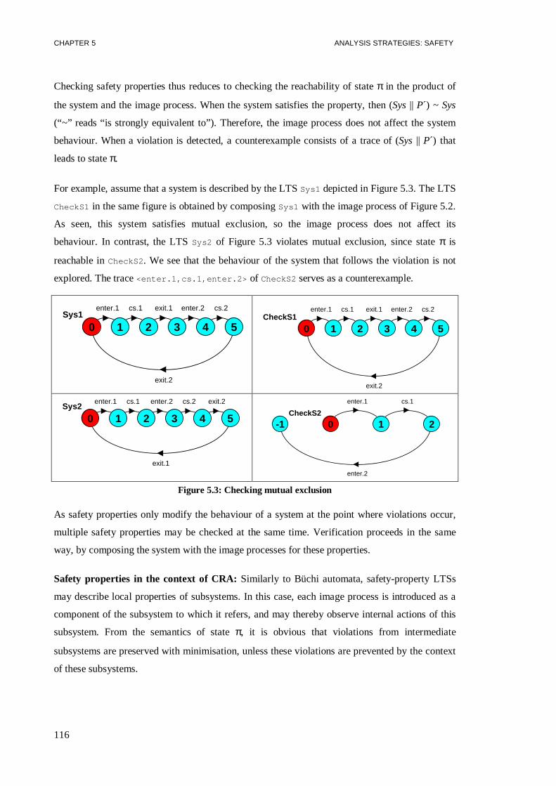
CHAPTER 5 ANALYSIS STRATEGIES: SAFETY
116
Checking safety properties thus reduces to checking the reachability of stateπ in the product of
the system and the image process. When the system satisfies the property, then (Sys|| P´) ~ Sys
(“~” reads “is strongly equivalent to”). Therefore, the image process does not affect the system
behaviour. When a violation is detected, a counterexample consists of a trace of (Sys|| P´) that
leads to stateπ.
For example, assume that a system is described by the LTSSys1 depicted in Figure 5.3. The LTS
CheckS1 in the same figure is obtained by composingSys1 with the image process of Figure 5.2.
As seen, this system satisfies mutual exclusion, so the image process does not affect its
behaviour. In contrast, the LTSSys2 of Figure 5.3 violates mutual exclusion, since stateπ is
reachable inCheckS2 . We see that the behaviour of the system that follows the violation is not
explored. The trace<enter.1,cs.1,enter.2> of CheckS2 serves as a counterexample.
Sys1enter.1 cs.1 exit.1 enter.2 cs.2
exit.2
0 1 2 3 4 5CheckS1
enter.1 cs.1 exit.1 enter.2 cs.2
exit.2
0 1 2 3 4 5
Sys2enter.1 cs.1 enter.2 cs.2 exit.2
exit.1
0 1 2 3 4 5CheckS2
enter.1 cs.1
enter.2
-1 0 1 2
Figure 5.3: Checking mutual exclusion
As safety properties only modify the behaviour of a system at the point where violations occur,
multiple safety properties may be checked at the same time. Verification proceeds in the same
way, by composing the system with the image processes for these properties.
Safety properties in the context of CRA: Similarly to Büchi automata, safety-property LTSs
may describe local properties of subsystems. In this case, each image process is introduced as a
component of the subsystem to which it refers, and may thereby observe internal actions of this
subsystem. From the semantics of stateπ, it is obvious that violations from intermediate
subsystems are preserved with minimisation, unless these violations are prevented by the context
of these subsystems.

CHAPTER 5 ANALYSIS STRATEGIES: SAFETY
117
Let Sys and Syssaf be the LTSs of a system computed with traditional CRA and TRACTA,
respectively. As described above,Syssaf is the LTS obtained by adding image processes in the
compositional hierarchy of the system, and performing CRA. Ifπ is reachable inSyssaf, then the
system violates some of its desired properties, and a trace to stateπ may be used as a
counterexample. Ifπ is not reachable, thenSyssaf satisfies the properties checked, in which case
Syssaf is identical toSys. This is becauseSyssaf andSysare the minimal versions of LTSs that are
strongly equivalent, where minimisation is performed with respect to weak equivalence.
Consequently, in the absence of safety property violations, the LTS obtained with our approach
correctly reflects the behaviour of the system. This LTS can be used for further verification,
interactive simulation (see Chapter 7) or even as a component in a larger system.
Safety property checking with image processes may significantly reduce the size of both the
intermediate and the final LTSs for a system, in the presence of property violations. This is
because traces of the system are not explored beyond violating (π) states. A limitation of the
approach is that the violation of any property is mapped to the same state,π. This means that
when multiple properties are introduced into analysis, it may be difficult to identify which
properties are violated by the system. In most cases, the counterexample trace leading to the
violation indicates the property that is being violated. If the counterexample does not identify a
property, then it may be used to track the violation in more primitive components of the
compositional hierarchy.
Describing safety properties in FSP:In FSP, property specifications are distinguished from
those of component behaviour with the keywordproperty . For example, the mutual exclusion
property described earlier is expressed in FSP as follows:
property MUT_EXCL = (enter[i:1..2] -> exit[i] -> MUT_EXCL).
Without the keyword property, this specification corresponds to the LTS of Figure 5.1. Being
specified as a property, it generates the image process of this LTS, shown in Figure 5.2. In the
context of analysis, a property LTS will be usually represented directly as its image process.
5.1.2 Correctness
In general, we call a processP transparentto a systemSys with respect to an equivalence
relationR between processes, iff (Sys|| P, Sys) ∈ R. Moreover, we say that an LTSP=⟨S, A, ∆, p⟩
is totally definediff stateπ is not reachable inP, which means thatπ∉S.

CHAPTER 5 ANALYSIS STRATEGIES: SAFETY
118
In [Giannakopoulou 95], we have proposed a “transparency theorem” that establishes sufficient
and necessary conditions for a process to be transparent to a system.
Transparency theorem:Let Z andP be two totally defined LTSs, whereP is deterministic and
free of internal actionτ. ThenZ ~ (Z ||P) iff:
1. αP ⊆ αZ;
2. tr(Z ↑ αP) ⊆ tr(P). ■
This theorem is a new version of the interface theorem introduced and used in [Cheung 94c,
Cheung and Kramer 95b, Cheung and Kramer 96a]. The transparency theorem refines the
interface theorem in two ways. Firstly, it restricts its applicability to LTSs that are totally defined
because, as proven in [Giannakopoulou 95], the interface theorem does not hold for LTSs where
π is reachable. As a result, the interface theorem cannot be directly used for proving that image
processes are transparent to a system. Secondly, unlike the conditions of the interface theorem,
those of the transparency theorem are both sufficient and necessary. We explain why this is
useful later in this section.
Image process theorem:Let P andQ be two totally defined processes, whereQ is deterministic
and free ofτ transitions withαQ ⊆ αP, and letQ´ be the image process ofQ. ThenP || Q´ is
totally defined ifftr(P ↑ αQ) ⊆ tr(Q). ■
The proofs of both theorems can be found in Appendix D where for the transparency theorem,
we additionally discuss why its conditions cannot be relaxed in the context of strong equivalence.
We now show how these theorems are used to prove the correctness of the mechanism for
checking safety properties presented in the previous section. LetP be a safety-property LTS that
expresses some property of a systemSys(P is a deterministic and free ofτ transitions LTS, with
αP ⊆αSys), andP´ be the image process ofP. Then:
SyssatisfiesP iff Sys||P´ is totally defined: From Definition 1,SyssatisfiesP iff tr(Sys↑αP) ⊆
tr(P). By the image process theorem,tr(Sys↑αP) ⊆ tr(P) iff Sys||P´ is totally defined.■
if SyssatisfiesP, thenP´ is transparent toSyswith respect to ~: From Definition 1,SyssatisfiesP
iff tr(Sys↑αP) ⊆ tr(P). From the transparency theorem,tr(Sys↑αP)⊆tr(P) iff ( Sys|| P) ~ Sys. As
proven above,SyssatisfiesP iff ( Sys || P´) is totally defined. But from the construction ofP´
from P, it is straightforward that when (Sys || P´) is totally defined, (Sys || P´)~(Sys || P).
Therefore, (Sys||P´) ~ (Sys|| P) ~ Sys, i.e. P´ is transparent to the system with respect to “~”.■

CHAPTER 5 ANALYSIS STRATEGIES: SAFETY
119
User-specified interfaces in CRA: User-specified interfaces are used in CRA for avoiding
intermediate state explosion (see Section 2.6.2). TRACTA handles interfaces that are deterministic
and contain noτ-transitions similarly to safety-property LTSs. During CRA, the image processI´
of an interfaceI is composed with the subsystem to whichI relates. ThenI is correct iff the
global LTS obtained with CRA is totally defined. This has been proven in [Giannakopoulou 95]
as follows. In general, we say thatI is correct iff it is transparent to the system with respect to
strong equivalence, i.e. iff (Sys || I) ~ Sys (strong equivalence ~ is the strongest notion of
equivalence and has been chosen in order to make the technique widely applicable). But from the
transparency theorem, (Sys|| I) ~ Sysiff tr(Sys↑I) ⊆ tr(I), and from the image process theorem
this is equivalent to (Sys|| I´) being totally defined.
As discussed in Section 2.6.2, the interface theorem can only be used to prove that the method
for checking the correctness of user-specified interfaces proposed by [Cheung and Kramer 95b,
Cheung and Kramer 96b] is conservative. With the transparency theorem, we have proven that
the method accepts exactly those interfaces that are correct.
5.1.3 Non-deterministic safety properties
The checking mechanism presented assumes that safety-property LTSs are deterministic. This is
not a prerequisite of our approach since any non-deterministic LTS can be transformed into an
equivalent deterministic LTS. The algorithm presented by [Hopcroft and Ullman 79] can be used
to perform this transformation.
NON_DET
a
a
b c0 1 2
DET
a
b
c
c b0 1 2 3
Figure 5.4: Transformation from non-deterministic to deterministic property LTS
Therefore, TRACTA can also handle non-deterministic LTSs, if they contain noτ-transitions.
These LTSs are translated into deterministic ones, which are then used as described in the
previous sections. For example, assume that we wish to check that, in the context of alphabet {a,
b, c}, the occurrence of actiona can be followed by either exclusivelyb-actions or exclusivelyc-
actions. If the designer specifies this property as the non-deterministic LTSNON_DETdepicted in
Figure 5.4, TRACTA transformsNON_DETinto the deterministic LTSDETof the same figure.

CHAPTER 5 ANALYSIS STRATEGIES: SAFETY
120
The algorithm that turns a non-deterministic automaton into a deterministic one has worst-case
complexity exponential in the size of the automaton. This is not a problem for property LTSs that
are small in size. However, users are advised to specify safety properties as deterministic LTSs.
Deterministic property LTSs avoid the overhead of the transformation, as well as being more
intuitive.
5.2 Alternating-bit protocol revisited
To illustrate our approach to safety-property checking, we use the example of the alternating-bit
protocol (ABP) presented in Chapter 3. As described, the protocol receiver ignores any message
that is tagged with a different value from the one it expects – the transmitter treats
acknowledgements in a similar way. In order to check the correctness of this mechanism for
identifying superfluous retransmissions of messages and acknowledgements, we introduce
propertyRIGHT_IGNOREthat refers to processRECEIVER. The FSP specification of the property
and the LTS generated from it are depicted in Figure 5.5.
RIGHT_IGNORE
ignore.1deliver.1
deliver.2
deliver.3
ignore.2ignore.3
ignore.1
deliver.1
deliver.2
deliver.3
ignore.2
ignore.3
ignore.1
deliver.1
deliver.2
deliver.3
ignore.2
ignore.3
-1 0 1 2
property RIGHT_IGNORE = MAY_IGNR[1], // initially at MAY_IGNR[1]
MAY_IGNR[i:VALUES]= ( ignore[i] -> MAY_IGNR[i]
| deliver[v:VALUES] -> MAY_IGNR[v]).
Figure 5.5: Property RIGHT_IGNORE of the ABP
PropertyRIGHT_IGNOREis designed to detect erroneous behaviour where the receiver ignores a
message that is not a duplicate. To this aim, it states that the receiver may only ignore a message
CHAPTER 5 ANALYSIS STRATEGIES: SAFETY
121
if it holds the same valuev as the latest message delivered by the receiver. Note that this
specification for propertyRIGHT_IGNOREallows the receiver to consider a new message as a
retransmission if that message contains the same value as the latest message delivered. However,
it is unnecessary to complicate the specification ofRIGHT_IGNORE to cover this case; if the
mechanism based on the tag-bit is erroneous,RIGHT_IGNORE will detect the problem when
successive messages hold different values.
An additional property that must hold on the system is the following:
property CORR_RES = (accept[v:VALUES] -> RESULT[v]),
RESULT[v:VALUES] = (result.ok[v] -> CORR_RES | result.failed -> CORR_RES).
PropertyCORR_RESstates that after accepting a message with valuev , the protocol reports on the
transmission result before a new value is accepted. Moreover, successful transmission must refer
to the same valuev that has been accepted (result.ok[v] ), i.e. the protocol must ensure that the
transmitter and receiver can correctly identify which acknowledgements and messages are
relevant for each round of the protocol.
TRACTA : As RIGHT_IGNOREcontains “ignore ” actions that are internal to the receiver, TRACTA
modifies the specification of componentRECEIVERas follows:
REC = REPLY[1][1],
DELIVER[b:BIT][x:VALUES] = (deliver[x] -> REPLY[b][x]),
REPLY[b:BIT][x:VALUES] = (reply[b][x] -> REPLYING[b][x]),
REPLYING[b:BIT][v:VALUES] = (rxto -> REPLY[b][v]
|rec[!b][x:VALUES] -> DELIVER[!b][x]
|rec[b][x:VALUES] -> ignore[x] -> REPLYING[b][v]).
|| RECEIVER = (REC || RIGHT_IGNORE)\ {rxto, ignore}.
RECEIVER is now a composite component (see Figure 5.6). ComponentREC has identical
behaviour to the initial receiver component, with the difference that actions{rxto, ignore} are
hidden after the receiver is combined with propertyRIGHT_IGNORE. ComponentRECin isolation
is not expected to satisfy the property. This is because the messages that it receives and their tag-
bits can acquire arbitrary values when the receiver is not in the context of the protocol. The
RECEIVERcomponent can thus exhibit, locally, erroneous behaviour leading to stateπ. However,
it requires to be used in systems that prevent such behaviour. PropertyCORR_RESis a global
property of the protocol. As it only involves globally observable actions, we compose it withABP
as follows:
|| CHECK_ABP= (ABP || CORR_RES).

CHAPTER 5 ANALYSIS STRATEGIES: SAFETY
122
trans:CHANNELtx:TRANSMITTER chnAck:CHANNEL rx:RECEIVER
utx:TRANS_CHNL urx:REC_CHNL
ABP
cnt:COUNTERpr_tx:PR_TX RIGHT_IGNOREREC
Figure 5.6: Compositional hierarchy for the ABP protocol
Traditional CRA: Traditional CRA only checks properties concerning globally observable
actions. In order to check propertyRIGHT_IGNORE, CRA must therefore expose all “ignore ”
actions of the receiver up to theABP component. To verify the correctness of the protocol, the
LTS for ABPthus obtained is composed with propertiesRIGHT_IGNOREandCORR_RESas follows:
|| CHECK_ABP= (ABP || CORR_RES || RIGHT_IGNORE).
Verification
The two versions of the protocol described in Section 3.3.1 have been verified using both
TRACTA and traditional CRA. As discussed above, in order to check the safety properties on this
protocol, both TRACTA and traditional CRA introduce some changes in the system. When a
modification is made in some subsystem, CRA-based methods only need to re-compute the
behaviour of the components affected by the change. The only components that are affected by
the change are the ones marked with block arrows in Figure 5.6. Therefore, the sizes of all
remaining components are as reported in Section 3.4.3. In the tables that display the sizes of the
LTSs obtained with TRACTA and CRA, we only display the modified components.
ABP – Version 1: The first version of the protocol (described in Section 3.3.1) satisfies
propertiesRIGHT_IGNORE and CORR_RES. Table 5.1 and Table 5.2 display the sizes of the
components of the system when performing analysis with TRACTA and traditional CRA,
respectively. The tables show that traditional CRA generates a larger LTS for theABP
component. This is despite the fact that with TRACTA, propertyRIGHT_IGNOREis included in the
behaviour ofABP. In fact, the minimised LTS obtained with TRACTA is identical to the one
obtained in Chapter 3. As discussed in Section 5.1.1, when a property LTS is satisfied, it does not
affect the behaviour of the system. The resulting LTS for the system may therefore be utilised for
further verification, interactive simulation, or as a component of larger systems.

CHAPTER 5 ANALYSIS STRATEGIES: SAFETY
123
We see that with TRACTA, both ABP and CHECK_ABPhave 7 states, as compared to traditional
CRA where they have 61 and 69 states, respectively. We conclude that, as a compositional
minimisation method, traditional CRA soon loses its capability of reducing the size of the system
as the number of internal actions that are involved in properties increases.
before minimisation after minimisationComponent#states #transitions #states #transitions
RECEIVER 48 84 19 55
REC_CHNL 73 229 55 163
ABP 108 246 7 9
CHECK_ABP 7 9 not necessary
Table 5.1: Version 1 of ABP checked with TRACTA
before minimisation after minimisationComponent#states #transitions #states #transitions
RECEIVER 36 72 36 72
REC_CHNL 102 270 84 210
ABP 210 504 61 132
CHECK_ABP 69 144 not necessary
Table 5.2: Version 1 of ABP checked with traditional CRA
ABP – Version 2: The second version of the protocol does not satisfy the properties
RIGHT_IGNOREandCORR_RES. As reported in Table 5.3 and Table 5.4, althoughABP contains an
additional component (i.e. the propertyRIGHT_IGNORE) in TRACTA, its LTS is smaller than that
obtained with traditional CRA. Moreover, as TRACTA detects the violation of property
RIGHT_IGNOREin the LTS of theABP, it does not compute the LTS ofCHECK_ABP.
TRACTA returned the following counterexample for theABPcomponent:
Trace to property violation:
<accept.1, result.failed, accept.2>
According to the software architecture of the protocol depicted in Figure 3.8, the “deliver ”
actions are globally observable, since they belong to the interface ofABP. As no “deliver ”
action appears in the counterexample returned, it means that no message is delivered before the
violation occurs. From the LTS of propertyRIGHT_IGNOREin Figure 5.5, and since the violation
happens after a message with value 2 is accepted (accept.2 ), the violation must be due to the
execution of transition (0, ignore.2, –1) of RIGHT_IGNORE. This shows that it is possible for the
receiver to ignore the receipt of value 2, before delivering it. We can then reconstruct the
following scenario based on the counterexample returned. According to the specification of the
protocol transmitter (Sections 3.3.2 and 3.3.3), messages are initially tagged with value 0.

CHAPTER 5 ANALYSIS STRATEGIES: SAFETY
124
Therefore, the transmitter tags with 0 the first message that it accepts (message holds value 1 –
accept.1 ), while the receiver also expects a message tagged with 0. After using up its
retransmission opportunities, the transmitter decides that the transmission of value 1 has failed
(result.failed ). The next message accepted (message holds value 2 –accept.2 ) is then tagged
with 1. However, the receiver still expects a message tagged with 0 and thereby ignores the
message with value 2 that is transmitted to it.
before minimisation after minimisationComponent#states #transitions #states #transitions
RECEIVER 48 84 19 55
REC_CHNL 73 229 55 163
ABP 4296 12538 not necessary
CHECK_ABP not necessary not necessary
Table 5.3: Version 2 of ABP checked with TRACTA
before minimisation after minimisationComponent#states #transitions #states #transitions
RECEIVER 36 72 36 72
REC_CHNL 102 270 84 210
ABP 6444 18636 2910 8586
CHECK_ABP 3702 10536 not necessary
Table 5.4: Version 2 of ABP checked with traditional CRA
As reported in Table 5.3, after detecting this problem in componentABP, there is no meaning in
checking other properties before the existing error in the design of the protocol is corrected. To
this aim, we have tried modifying the behaviour of the transmitter so that, after a failed delivery
of a message tagged withb, the next message is tagged with the same value. This is how the
transmitter is specified by [Valmari 93b], for this version of the protocol. Despite the change, the
violation remains. This error was not detected by [Valmari 93b].
From the analysis results discussed, we conclude that the problem with version 2 of ABP cannot
be remedied without changing the philosophy of the protocol. The receiver and transmitter need
to correctly decide when a transmission round starts for a new message, in order to change tag-
bits accordingly. To achieve this, the receiver must in some way be notified whenever the
transmitter decides that the current transmission has failed. This essentially reduces to reliable
communication over unreliable channels between the transmitter and the receiver, the initial
problem that the protocol itself is designed to solve.

CHAPTER 5 ANALYSIS STRATEGIES: SAFETY
125
Discussion
The fact that traditional CRA may need to expose actions at the global system has several
disadvantages. Firstly, it requires careful modification of the interfaces of subsystems in order to
make these actions globally observable. This can be performed directly on the FSP expressions
that describe components of the system. Alternatively, one may modify the component interfaces
in the software architecture (only for the behavioural view), and then re-generate FSP
expressions accordingly. However, such changes may need to be applied each time the developer
identifies new properties to be checked on the system. Secondly, the key to reduction with
compositional minimisation is to employ a modular software architecture and hide as many
internal actions as possible in each subsystem. Exposing internal actions at the global level
compromises the effectiveness of such techniques.
By appropriately introducing properties in the compositional hierarchy of the system, TRACTA
avoids globally exposing internal actions of subsystems. As subsystems contain their local
properties, they can be viewed as components that carry their correctness criteria. Some of the
subsystems may grow in size because of this fact (see for example componentRECEIVER in
Tables 1–4). This is not a disadvantage since, with traditional CRA, these properties need to be
composed with the final system anyway. Moreover, as stateπ prunes subsystem behaviour that
stems from safety property violations, TRACTA usually generates smaller (sub)systems as
compared to traditional CRA. Our examples show that this particularly happens as we move
towards higher-level components in the compositional hierarchy. Finally, in the global LTS
generated with TRACTA, the actions that are observable correspond exactly to the interface of the
system.
5.3 Safety properties as ALTL formulas
Assume that we wish to express propertyRIGHT_IGNOREof the ABP as an ALTL formula, and
check it with Büchi automata, as presented in Chapter 4. In ALTL, propertyRIGHT_IGNOREcan
be expressed as the conjunction of three propertiesf1, f2, f3, one for each value transmitted by the
protocol. Eachfi states that, after a valuei is delivered, no valuej≠i may be ignored until a new
valuek≠i is delivered. Propertyf1 can be expressed by the following ALTL formula:
f1 = □(deliver.1⇒ ((¬ignore.2∧ ¬ignore.3)Uw (deliver.2∨ deliver.3))).
Formulasf2 andf3 are defined similarly, and propertyRIGHT_IGNOREis expressed as (f1 ∧ f2 ∧ f3).
As discussed in Chapter 2, the size of a Büchi automaton for a property may be related
exponentially to the length of the formula. Therefore, it is preferable to checkRIGHT_IGNOREby

CHAPTER 5 ANALYSIS STRATEGIES: SAFETY
126
checkingf1, f2, andf3 individually. However, as these properties are symmetrical, we can argue
that it is sufficient to check the protocol against one of them, sayf1. To perform this, we build a
Büchi automatonWRONG_IGNOREthat corresponds to¬f1:
¬f1 = ◊ ¬(deliver.1⇒ ((¬ignore.2∧ ¬ignore.3)Uw (deliver.2∨ deliver.3)))
= ◊ (deliver.1∧ ¬((¬ignore.2∧ ¬ignore.3)Uw (deliver.2∨ deliver.3))).
The automatonWRONG_IGNOREis specified in FSP as described in Figure 5.7. The symbol “@”
marks the identifier of a process (possibly auxiliary), whose initial state corresponds to an
accepting state. As illustrated in Figure 5.7, the FSP specification of a Büchi automaton generates
directly the corresponding Büchi process. Figure 5.7 shows thatWRONG_IGNOREaccepts an
infinite word if actions ignore.2 or ignore.3 may occur after the delivery of value 1
(deliver.1 ), and before the delivery of any different value (deliver.2 , deliver.3 ).
WRONG_IGNORE
deliver.2deliver.3ignore.2ignore.3
deliver.1
deliver.2deliver.3
ignore.2ignore.3
deliver.1 deliver.2deliver.3ignore.2ignore.3deliver.1@WRONG_IGNORE
0 1 2
WRONG_IGNORE= ({deliver[2], deliver[3], ignore[2], ignore[3]} -> WRONG_IGNORE
|deliver[1] -> INTERM),
INTERM = (deliver[1] -> INTERM
|{ignore[2], ignore[3]} -> ACC
|{deliver[2], deliver[3]} -> WRONG_IGNORE),
ACC@ = ({deliver[i:VALUES], ignore[2], ignore[3]} -> ACC).
Figure 5.7: Büchi process for property WRONG_IGNORE
We analysed the first version of the ABP again, with TRACTA. However, this time,
WRONG_IGNOREwas used instead ofRIGHT_IGNORE, which means thatWRONG_IGNOREreplaced
RIGHT_IGNORE in the compositional hierarchy of Figure 5.6. As expected, the property is
satisfied. Table 5.5 presents the sizes of the subsystems affected by the introduction of the
property, as compared to their sizes whenRIGHT_IGNOREis used instead. Despite the fact that
RIGHT_IGNOREcovers all off1, f2andf3, whereasWRONG_IGNOREis limited to propertyf1, and even
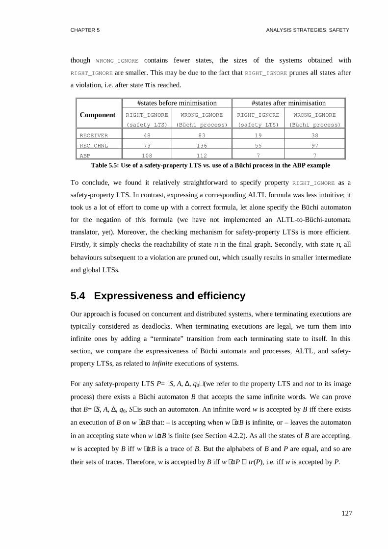
CHAPTER 5 ANALYSIS STRATEGIES: SAFETY
127
though WRONG_IGNOREcontains fewer states, the sizes of the systems obtained with
RIGHT_IGNOREare smaller. This may be due to the fact thatRIGHT_IGNOREprunes all states after
a violation, i.e. after stateπ is reached.
#states before minimisation #states after minimisation
Component RIGHT_IGNORE
(safety LTS)
WRONG_IGNORE
(Büchi process)
RIGHT_IGNORE
(safety LTS)
WRONG_IGNORE
(Büchi process)
RECEIVER 48 83 19 38
REC_CHNL 73 136 55 97
ABP 108 112 7 7
Table 5.5: Use of a safety-property LTS vs. use of a Büchi process in the ABP example
To conclude, we found it relatively straightforward to specify propertyRIGHT_IGNORE as a
safety-property LTS. In contrast, expressing a corresponding ALTL formula was less intuitive; it
took us a lot of effort to come up with a correct formula, let alone specify the Büchi automaton
for the negation of this formula (we have not implemented an ALTL-to-Büchi-automata
translator, yet). Moreover, the checking mechanism for safety-property LTSs is more efficient.
Firstly, it simply checks the reachability of stateπ in the final graph. Secondly, with stateπ, all
behaviours subsequent to a violation are pruned out, which usually results in smaller intermediate
and global LTSs.
5.4 Expressiveness and efficiency
Our approach is focused on concurrent and distributed systems, where terminating executions are
typically considered as deadlocks. When terminating executions are legal, we turn them into
infinite ones by adding a “terminate” transition from each terminating state to itself. In this
section, we compare the expressiveness of Büchi automata and processes, ALTL, and safety-
property LTSs, as related toinfinite executions of systems.
For any safety-property LTSP= ⟨S, A, ∆, q0⟩ (we refer to the property LTS andnot to its image
process) there exists a Büchi automatonB that accepts the same infinite words. We can prove
thatB= ⟨S, A, ∆, q0, S⟩ is such an automaton. An infinite wordw is accepted byB iff there exists
an execution ofB on w αB that: – is accepting whenw αB is infinite, or – leaves the automaton
in an accepting state whenw αB is finite (see Section 4.2.2). As all the states ofB are accepting,
w is accepted byB iff w αB is a trace ofB. But the alphabets ofB andP are equal, and so are
their sets of traces. Therefore,w is accepted byB iff w αP ∈ tr(P), i.e. iff w is accepted byP.
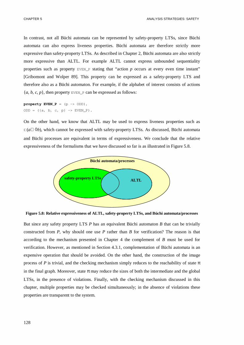
CHAPTER 5 ANALYSIS STRATEGIES: SAFETY
128
In contrast, not all Büchi automata can be represented by safety-property LTSs, since Büchi
automata can also express liveness properties. Büchi automata are therefore strictly more
expressive than safety-property LTSs. As described in Chapter 2, Büchi automata are also strictly
more expressive than ALTL. For example ALTL cannot express unbounded sequentiality
properties such as propertyEVEN_P stating that “actionp occurs at every even time instant”
[Gribomont and Wolper 89]. This property can be expressed as a safety-property LTS and
therefore also as a Büchi automaton. For example, if the alphabet of interest consists of actions
{ a, b, c, p}, then propertyEVEN_Pcan be expressed as follows:
property EVEN_P = (p -> ODD),
ODD = ({a, b, c, p} -> EVEN_P).
On the other hand, we know that ALTL may be used to express liveness properties such as
□(a⇒◊b), which cannot be expressed with safety-property LTSs. As discussed, Büchi automata
and Büchi processes are equivalent in terms of expressiveness. We conclude that the relative
expressiveness of the formalisms that we have discussed so far is as illustrated in Figure 5.8.
safety-property LTSs
Büchi automata/processes
ALTL
Figure 5.8: Relative expressiveness of ALTL, safety-property LTSs, and Büchi automata/processes
But since any safety property LTSP has an equivalent Büchi automatonB that can be trivially
constructed fromP, why should one useP rather thanB for verification? The reason is that
according to the mechanism presented in Chapter 4 the complement ofB must be used for
verification. However, as mentioned in Section 4.3.1, complementation of Büchi automata is an
expensive operation that should be avoided. On the other hand, the construction of the image
process ofP is trivial, and the checking mechanism simply reduces to the reachability of stateπ
in the final graph. Moreover, stateπ may reduce the sizes of both the intermediate and the global
LTSs, in the presence of violations. Finally, with the checking mechanism discussed in this
chapter, multiple properties may be checked simultaneously; in the absence of violations these
properties are transparent to the system.

CHAPTER 5 ANALYSIS STRATEGIES: SAFETY
129
5.5 Summary
In this chapter, we have presented an efficient mechanism for checking safety properties
expressed as LTSs. The traces of a property LTS describe all the legal traces that a system may
exhibit, when restricted to the alphabet of this LTS. The mechanism is based on a very simple
transformation of a property LTS into its image process, performed by replacing all undefined
transitions of the LTS with transitions to the error state,π. The image process is introduced in the
compositional hierarchy of the system under verification, as a component of the (sub)system to
which it refers. As such, it may contain actions of the subsystem that are not globally observable.
Analysis then consists of performing CRA to compute the LTS of the system, and checking if
state π is reachable in this LTS. Ifπ is reachable, then the property is violated and a
counterexample is returned. This approach to checking safety properties has a number of
advantages:
1. multiple properties may be checked simultaneously;
2. it may reduce the sizes of the system and subsystems in the presence of property violations;
3. it consists of a simple check for the reachability of stateπ;
4. in the absence of violations, the properties are transparent to the system. This means that the
global LTS obtained correctly reflects the behaviour of the system, and may be used for
further verification, interactive simulation, or as a component of larger systems.
A limitation of the approach is that the violation of any property is mapped to the same state,π.
This means that, when checking multiple properties, it may be difficult to identify which ones are
violated. In most cases the counterexample trace leading to the violation indicates the property
that is being violated. If the counterexample does not identify the property, then it may be used to
track the violation in more primitive components of the compositional hierarchy.
The safety-checking mechanism has been illustrated on the two versions of the alternating-bit
protocol described in Chapter 3, and has helped us detect that the second version is problematic.
In addition, the approach has been compared to traditional CRA and to ALTL model checking.
We have closed the chapter by discussing the relative expressiveness of the various formalisms
for specifying system properties presented so far, that is, Büchi automata and processes, ALTL,
and safety-property LTSs.

130

131
Analysis Strategies: Liveness 66.1 FAIRNESS CONSIDERED 131
6.2 ADDING FAIRNESS CONSTRAINTS TO PROCESS BEHAVIOUR 134
6.3 FAIR CHOICE 136
6.4 PROGRESS PROPERTIES 141
6.5 EXAMPLE: READERS-WRITERS 144
6.6 DISCUSSION 147
6.7 DETERMINISTICBÜCHI AUTOMATA 148
6.8 GENERAL METHODOLOGY 150
6.9 SUMMARY 151
In Chapter 5, we mentioned that for some classes of properties or under specific assumptions on
the behaviour of a system, model checking is amenable to strategies that do not suffer from the
disadvantages of our generic mechanism. This chapter proposes such strategies for checking
liveness properties of a system. In this context, we also introduce the notion of fairness, and
discuss how fairness assumptions affect liveness property checking.
6.1 Fairness considered
Liveness and fairness are two closely related issues in program verification. When checking
liveness in a program and no notion of fairness has been assumed or incorporated in the model,
the results obtained from verification require to be filtered to a large extent. For example, one
cannot expect that processes of a concurrent program will never starve, when the program runs
on a system with a scheduling policy that does not implement any kind of fairness. Liveness
property violations that are caused by such circumstances are not of interest to the developer.
For example, consider the LTS of Figure 6.1 that represents the joint behaviour of a server and
two clientsA and B accessing it. At start-up, the server gets initialised, and then enters a state
where it is ready to receive requests from its clients. After receiving a request (a.req or b.req ),
the server delays for some arbitrary time while processing it, and then produces a reply to the
client that made the request (a.reply or b.reply , respectively). One expects that in any
execution of this system, each client is able to regularly communicate with the server. This
means that botha.req and b.req occur infinitely often in any system execution, or, more

CHAPTER 6 ANALYSIS STRATEGIES: LIVENESS
132
formally, that the system satisfies the following two liveness properties:fa=(□◊a.req ) and
fb=(□◊b.req ). But the LTS of systemCL_SERmay generate the following execution:
“ 0 initialise 1 (a.req 3 delay 3 a.reply 1)ω ”
that obviously violatesfb, since b.req never occurs in it. This violation corresponds to a
scheduler that is consistently biased against transition (1, b.req, 2 ), when given a choice.
However, any reasonable scheduler should implement some notion of fairness when choosing
between sets of possible transitions.
CL_SER
initialise
a.req
b.req
b.reply
delay
a.reply
delay0 1 2 3
SERVER= (initialise -> SERVE),
SERVE = ( a.req ->DEL1 | b.req -> DEL2),
DEL1 = (delay -> DEL1 | a.reply->SERVE),
DEL2 = (delay -> DEL2 | b.reply->SERVE).
A = (a.req -> a.reply -> A).
B = (b.req -> b.reply -> B).
||CL_SER = (A || B || SERVER).
Figure 6.1: A simple client-server system
Fairness imposes additional restrictions on the computations allowed by a model in order to
exclude computations that do not correspond to actual executions of real concurrent systems
[Manna and Pnueli 92]. [Lehmann, et al. 81] have proposed three notions of fairness that are
useful in practice, namelyweak, strong, andunconditionalfairness. These are also referred to as
justice, fairness (or compassion) and impartiality, respectively [Manna and Pnueli 92].
Let P = ⟨S, A, ∆, q0⟩ be the LTS of a program. We say that a transition (s, a, s )∈∆ is enabledat a
states1∈S iff s1 = s. For an executionσ = q0a0q1a1… of P, we say∀i≥0 that transition (qi, ai, qi+1)
occurs in the execution. A transitiont is enabled at a stateqi in σ iff t is enabled atqi in P. A
transitiont is enabledcontinuouslyfrom qi in σ, iff t is enabled at all statesqj in σ such thatj ≥ i.
Finally, at stateqi in σ, it holds that transition (s, a, s ) eventually occurs iff∃ j ≥ i such that
(s,a,s ) = (qj, aj, qj+1).
CHAPTER 6 ANALYSIS STRATEGIES: LIVENESS
133
An executionσ is:
• weakly fair iff at every state inσ it holds that, if some transitiont∈∆ is enabled
continuously from this state, thent eventually occurs. In other words, at any point inσ a
transitiont eventually occurs, unlesst is eventually disabled. Consequently, any transitiont
occurs infinitely often inσ unlesst is disabled infinitely often.
• strongly fair iff for every transitiont∈∆, if t is enabled infinitely often inσ, the t also
occurs infinitely often. In other words, a transitiont occurs infinitely often inσ, unless there
is a point after whicht remains permanently disabled.
• unconditionally fairiff all transitions in∆ occur infinitely often inσ.
Let us apply these definitions to the LTS of Figure 6.1. Weak fairness excludes from this LTS all
executions where the server takes infinite time to process a request. For example, the execution:
“0 initialise 1 b.req 2 (delay 2)ω ”
is not weakly fair because wherever state2 occurs, transition (2, b.reply, 1 ) is enabled
continuously from there on, but it does not eventually occur. However, weak fairness allows
executions where the server listens to requests of one client only, and consistently ignores the
requests of the other client. Strong fairness excludes such executions. Any infinite execution goes
through state1 infinitely often. As both (1, a.req, 3 ) and (1, b.req, 2 ) are enabled at state1,
these transitions must also occur infinitely often. Finally, unconditional fairness expects all
transitions to occur infinitely often.CL_SER cannot generate any unconditionally fair execution
since there is no way of making transition (0, initialise, 1 ) occur infinitely often. For this
example, only strong fairness restricts the executions of the LTS as required.
Clearly, for any LTSP, it holds that: {unconditionally fair executions ofP} ⊆{strongly fair
executions ofP} ⊆ {weakly fair executions ofP} ⊆ {executions ofP}. In the definitions of
weak, strong, and unconditional fairness, the term “transition” can be substituted by “process” or
“action” to obtain the same fairness conditions with respect to processes [Clarke, et al. 86] or
actions [Lamport 94]. For example, assume that a concurrent system is scheduled in a strongly
fair way with respect to processes. Then in every execution of this system, if a process is enabled
infinitely often, it also “occurs” (i.e. executes) infinitely often. Fairness with respect toprocesses
cannot easily be incorporated in CRA approaches; as soon as processes are composed,
concurrency can no longer be distinguished from choice between operations of a single process.

CHAPTER 6 ANALYSIS STRATEGIES: LIVENESS
134
This could only be achieved by modifying the LTSs of the system components to record all
necessary information, similarly to the approach proposed by [Clarke, et al. 86].
In general, it is difficult to select a generic notion of fairness that achieves the desirable results
for all the systems of interest. Moreover, different notions of fairness are appropriate for different
system models. [Apt, et al. 88] present some criteria of effectiveness and utility of adopting some
notion of fairness in a computational model. [Queille and Sifakis 83] deal with fairness
extensively, and stress the importance of defining fairness with respect to specific actions or
predicates of the system. They call thisrelative fairness. [Natarajan and Cleaveland 95] take such
an approach, and propose a notion of weak fairness with respect tosuccess, in order to determine
when a process passes a test. Similarly, the framework presented by [Manna and Pnueli 92]
supports the specification of weak and strong fairness with respect to specific transitions in the
system. Finally in Unity, the notion of fairness requires that every statement is selected infinitely
often in any infinite execution [Chandy and Misra 88]. A good overview of fairness can be found
in [Francez 86].
6.2 Adding fairness constraints to process behaviour
A way of dealing with fairness in model checking is to add Büchi acceptance conditions to the
system. For example in [Aggarwal, et al. 90], the components of a system are modelled as Büchi
automata, and only accepting executions of their product automaton are checked for correctness.
[Gribomont and Wolper 89] describe how a Büchi automaton can be used to express a fair
process scheduler. [Clarke, et al. 86] extend their Kripke models with a set of predicates, so that
fair paths are defined as paths in which each predicate holds infinitely often. This is equivalent to
turning the model of the system into a generalised Büchi automaton. In this way, they can
express both weak and unconditional fairness with respect to processes. However, this requires
the user to modify the initial model of the system.
In TRACTA, Büchi processes can be included in the system in order to imposefairness
constraints. For example, consider the simple client-server systemCL_SER illustrated in Figure
6.1. The constraint thata.req andb.req must occur infinitely often in any reasonable execution
of CL_SERcan be expressed with the Büchi processFAIR_SERVE of Figure 6.2. By Theorem 4.1,
the product of two Büchi processes accepts the intersection of their languages. Therefore, the
accepting executions ofCL_SER||FAIR_SERVE correspond to thefair executions ofCL_SERover
its alphabet. This is because, in accepting executions ofCL_SER||FAIR_SERVE , both a.req and
b.req occur infinitely often, since both@Aand@Bmust be enabled infinitely often.

CHAPTER 6 ANALYSIS STRATEGIES: LIVENESS
135
FAIR_SERVE
tau
tau
a.req
@A
b.req
@B0 1 2
Figure 6.2: Using Büchi processes to impose fairness constraints
For verification, Büchi processes for constraints and properties of the system are treated in a
uniform way. The LTSP of a system is composed both with the Büchi processes that express
fairness constraints, and with the Büchi process for the negation of a desired propertyf. The
resulting Büchi processResaccepts the intersection of their languages. This means that the
accepting executions ofResover αRescorrespond to thefair executions ofP that satisfy the
negation of the property. Model checking then consists of checking ifRes is empty, which
implies that allfair executions ofP satisfyf.
b.crash
initialise
a.req
b.req
b.crash a.req
a.reply
delay
b.reply
delay
a.reply
b.crash
delay
initialise
0 1 2 3 4 5 6
Figure 6.3: System consisting of a server and two clients, one of which may crash
Consider now the case where in theCL_SERsystem, clientB is substituted by clientB_FAULTYthat
may crash as modelled by the following FSP expression:
B_FAULTY = (b.req->b.reply->B_FAULTY | b.crash->STOP).

CHAPTER 6 ANALYSIS STRATEGIES: LIVENESS
136
For simplicity, we assume thatB_FAULTY does not crash while waiting for a reply. The modified
CL_SER system is depicted in Figure 6.3. Adding constraintFAIR_SERVE to this system would
introduce the possibility of deadlock. For example, a deadlock state corresponds toCL_SERbeing
in local state2 and FAIR_SERVE in local state2. It is reached if B_FAULTY crashes while
FAIR_SERVEexpects a request from it. [Gribomont and Wolper 89] report a similar problem with
their model of a fair scheduler, when the processes of a system may block.
In general, the process of identifying and explicitly specifying fairness constraints is
complicated, highly depends on the specific system, and adds a large overhead to system
modelling. Moreover, the state space of models can increase dramatically with the composition
of Büchi fairness constraints, which exacerbates the state-explosion problem. This approach to
modelling fairness is therefore impractical in most cases.
6.3 Fair choice
As discussed, it is not possible to express fairness in the standard LTS model, unless Büchi
constraints are introduced to it. As a simpler alternative, we propose to add the option of making
a simple fairness assumption on the LTS model, which we refer to asfair choice.
Fair Choice: If a choice over a set of transitions is executed infinitely often, then every transition
in the set is executed infinitely often.■
Fair choice is equivalent to strong fairness with respect to the transitions of a system. This can be
realised by the fact that a transition is enabled infinitely often iff a choice over this transition is
executed infinitely often. However, we prefer to use the term “fair choice” because it reflects our
assumption in a more direct way.
6.3.1 Checking liveness under fair choice
The TRACTA liveness-checking mechanisms are simplified when the system executes under fair
choice. This result is based on the Terminal-Set Theorem described below. Before presenting the
theorem, we introduce some terms that will be used.
A states ´ is reachablefrom a states in an LTSP = ⟨S, A, ∆, q0⟩, iff (( s ´ = s) or (∃a∈A and
∃s ∈S, such that (s, a, s )∈∆ and s ´ is reachable froms )). For a states∈S, Reachable(s, P)
denotes the set of states that are reachable froms in P, i.e. Reachable(s, P) ={ s ∈S | s is
reachable froms in P}.

CHAPTER 6 ANALYSIS STRATEGIES: LIVENESS
137
Definition 1 – A terminal set of states C⊆S in an LTSP = ⟨S, A, ∆, q0⟩ is a strongly-connected
component with no outgoing transitions, i.e.
• ∀s∈C, C ⊆ Reachable(s, P)), and
• ∀s∈C, Reachable(s, P) ⊆ C. ■
It follows directly from the above definition that a set of states in an LTSP is terminal iff ∀s∈C,
Reachable(s, P) = C.
Terminal-Set Theorem -Let P = ⟨S, A, ∆, q0⟩ be an LTS that executes under “fair choice”. Ifw
is a legal infinite execution ofP, then the states that appear infinitely often inw form a terminal
set of states inP.
Proof: Let S1 ⊆ Sbe the set of states that appear infinitely often inw. SinceP consists of a finite
number of states, thenS1 is not empty. With fair choice, the fact that states inS1 are repeated
infinitely often in w implies that all transitions that are enabled at these states also occur
infinitely often in w. This means that all states that are reachable from states ofS1 in P occur
infinitely often in w. We conclude that∀s∈S1, Reachable(s, P) ⊆ S1. It is also straightforward
that since all states inS1are repeated infinitely often inw, then every state inS1 is reachable from
any other state inS1, and therefore∀s∈S1, S1 ⊆ Reachable(s, P). We conclude that∀s∈S1,
Reachable(s, P) = S1 and thereforeS1 is a terminal set of states.■
The Terminal-Set Theorem shows that a fair infinite executionw of an LTS is obtained by
repeating infinitely often the states of a terminal set of states. Similarly, a Büchi process
executing under fair choice is non-empty iff it contains a terminal set of states where all its
accepting actions are enabled. Therefore, when fair choice is assumed, the model-checking
mechanisms presented so far need only consider theterminal sets of statesin a graph, rather than
the non-transient strongly-connected components. Terminal sets are found by computing the
strongly-connected components in the graph and applying the additional criterion that no
transition exists from a state of the strongly connected component to a state outside it.
We call a Büchi processcompleteif all actions in its alphabet that are not accepting are enabled
at every state. When fair choice is assumed, the Büchi processes that are used for model-
checking must be complete. Otherwise, a strongly-connected component with outgoing
transitions in the LTS may become a terminal set of states in the product of the LTS with the
Büchi process; this occurs when the Büchi process prevents the occurrence of the outgoing
transitions. The fact that Büchi processes must be complete is not a problem in practice.

CHAPTER 6 ANALYSIS STRATEGIES: LIVENESS
138
Similarly to Büchi automata [Fernandez, et al. 92a], a Büchi processB can always be made
complete by adding a new state “s”. For each actiona∈αB (not including accepting actions) and
for each stateq in B (including the new states), if a is not enabled atq then (q, a, s) is added to
processB. Since no accepting action is enabled ats, s corresponds to a non-accepting state.
In Chapter 4, we mentioned that observational equivalence does not preserve non-transient
strongly-connected components in a graph. In contrast, terminal sets of states are preserved. As
there are no transitions from any state of a terminal set of statesTSSto a state outside it,
observational equivalence maps the states ofTSS to states that form a terminal set in the
minimised graph. This could be a terminating state, but such states are also considered as
terminal sets, according to Definition 1. Note that the deadlocks in a system are corrected before
checking other properties; therefore, at this stage, terminating states do not reflect deadlock, but
rather someτ-cycle that has disappeared with minimisation.
We conclude that hiding and minimisation preserve liveness property violations by fair
executions of a system. Fair choice greatly simplifies liveness checks with CRA, as the use of the
RD algorithm is not required. In the presence of a violating terminal set of statesC in the global
system, the diagnostic information returned by our tools consists of a trace leading to some state
in C, and the set of observable actions enabled inC.
6.3.2 Action priority
A great advantage of fair choice is the simple way in which property checking is introduced in
CRA. Fair choice detects situations where a system violates a property, even under the most
favourable conditions. Admittedly, such violations are vital to detect in a system. However, fair
choice is often too restrictive to be practical. In fact, practical schedulers in computing systems
do not implement strong fairness [Andrews 91, Queille and Sifakis 83]. This means that some
executions that may be exhibited by a system will be ignored by our checking mechanism as
unfair. Even so, the simplicity of the test makes it a good candidate for an initial coarse-grained
analysis. To achieve a better coverage of the violations in a system, we propose a simple action
priority scheme that allows the user to “stress” a system by applying adverse scheduling
conditions [Giannakopoulou, et al. 98a].
TRACTA supports alow and ahigh priority operator, denoted as “>>” and “<<”, respectively.
These take as arguments an LTSP and a set of actionsK⊆Actτ (accepting actions cannot be
included inK). The LTSsP>>K andP<<K have the same states, initial state, and alphabet asP,
but their transition relations may be different.P>>K expresses the fact that actions inK have
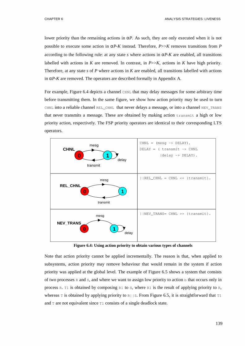
CHAPTER 6 ANALYSIS STRATEGIES: LIVENESS
139
lower priority than the remaining actions inαP. As such, they are only executed when it is not
possible to execute some action inαP-K instead. Therefore,P>>K removes transitions fromP
according to the following rule: at any states where actions inαP-K are enabled, all transitions
labelled with actions inK are removed. In contrast, inP>>K, actions inK have high priority.
Therefore, at any states of P where actions inK are enabled, all transitions labelled with actions
in αP-K are removed. The operators are described formally in Appendix A.
For example, Figure 6.4 depicts a channelCHNLthat may delay messages for some arbitrary time
before transmitting them. In the same figure, we show how action priority may be used to turn
CHNLinto a reliable channelREL_CHNL that never delays a message, or into a channelNEV_TRANS
that never transmits a message. These are obtained by making actiontransmit a high or low
priority action, respectively. The FSP priority operators are identical to their corresponding LTS
operators.
CHNLmesg
transmit
delay0 1
CHNL = (mesg -> DELAY),
DELAY = ( transmit -> CHNL
|delay -> DELAY).
REL_CHNL
mesg
transmit
0 1
||REL_CHNL = CHNL << {transmit}.
NEV_TRANS
mesg
delay0 1
||NEV_TRANS= CHNL >> {transmit}.
Figure 6.4: Using action priority to obtain various types of channels
Note that action priority cannot be applied incrementally. The reason is that, when applied to
subsystems, action priority may remove behaviour that would remain in the system if action
priority was applied at the global level. The example of Figure 6.5 shows a system that consists
of two processesR andS, and where we want to assign low priority to actionb that occurs only in
processR. T1 is obtained by composingR1 to S, whereR1 is the result of applying priority toR,
whereasT is obtained by applying priority toR||S . From Figure 6.5, it is straightforward thatT1
andT are not equivalent sinceT1 consists of a single deadlock state.

CHAPTER 6 ANALYSIS STRATEGIES: LIVENESS
140
When applied to a system that is not composed further, action priority does not introduce non-
existing deadlocks to the system, since it only removes behaviour when an alternative can be
selected. In the context of CRA, action priority can be applied to subsystems, but only in order to
check them in isolation. These “test” subsystems are not used in constructing composite
behaviours, since the application of action priority removes parts of system behaviour. For
system construction, action priority is only introduced at the top level of the compositional
hierarchy, i.e. when the global behaviour of the system is computed.
Our tools apply action priorityduring the construction of a composite process. Therefore, action
priority can also be used to perform a partial search on a system that is too large to explore
exhaustively. In such cases, action priority provides a way of selecting interesting behaviours for
analysis. However, when an exhaustive search is possible, safety analysis must be performed
before action priority is applied; as action priority removes transitions, it may also remove
erroneous system behaviour.
R
a
b
a
c
0 1
R = (a->R | b-> I),
I = (a->I | c-> R).
Tb c
a
0 1 2
||T = (R || S) >> {b}.
R1
a0
||R1 = R >> {b}.
S
c
a
0 1
S = (c->a->S). T1
0
||T1 = (R1 || S).
Figure 6.5: Action priority is not compositional
Related work: The notion of priority has been introduced as a means of assigning more
importance to some actions than others. Examples of actions that require special treatment are
interrupts and timeouts. [Phillips 94] performs a study and comparison between various
approaches to introducing priority in process algebra. Relative vs. absolute and conditional vs.
exclusive forms of priority appear in the literature. Recently, dynamic priority has also been
proposed in the context of real-time systems [Bhat, et al. 97]. In our approach, priority is not used
as a modelling operator. Rather, it is simply used as a way of eliminating transitions, and

CHAPTER 6 ANALYSIS STRATEGIES: LIVENESS
141
checking system executions under fair choice that would otherwise be considered unfair.
Therefore, the semantic equivalence of our model need not remain a congruence with the
introduction of a priority scheme. For this reason, we have taken a very simple approach to
priority, similar to the initial one proposed by [Cleaveland and Hennessy 90].
6.4 Progress properties
The regular occurrence of some actions in a system execution indicates that system behaviour
progresses as desired or expected. We would therefore like to be able to check on the model of a
system that, in all possible executions of the system, such actions occur regularly. In the context
of an infinite execution, regularly means infinitely often. A property asserting that an actiona is
expected to occur infinitely often in every infinite execution of the system is expressed in ALTL
as□◊a. We call properties of this typeprogress[Giannakopoulou, et al. 98a]. Often, progress is
not determined by a single action but by one of a set of alternatives. For example, a system may
be considered to make progress if it outputs one of a set of values. In FSP, we define progress
properties in terms of a finite set of actions as follows:
progress P = {a 1,a 2..a n} defines a progress propertyP which asserts that in
any infinite execution of a target system, at least one of the actionsa1,a 2..a n
occurs infinitely often.
Progress properties are a subclass of properties that can be expressed as ALTL formulas. The
ALTL formulation of progress propertyP is □◊(a1 ∨ a2 … ∨ an).
For example, let us return to the simple client-server systemCL_SER described in Section 6.1,
where the LTS of the system is depicted in Figure 6.1. Users would expect this system to satisfy
both propertiesga=( □◊a.reply) and gb=( □◊b.reply) , which state that the two clients are
served infinitely often in any infinite execution of the system. These properties can be specified
in FSP asSERVE_A={a.reply} and SERVE_B={b.reply} , which are satisfied under fair choice.
However, when clientB_FAULTY substitutes clientB, we can see from Figure 6.3 that progress
property SERVE_B is no longer satisfied. The following counterexample is produced by our
analysis tools:
Progress violation: SERVE_B
Trace to terminal set of states: < b.crash, initialise >
Actions in terminal set:
{a.req, a.reply, delay}

CHAPTER 6 ANALYSIS STRATEGIES: LIVENESS
142
The trace<b.crash, initialise> leads the LTS of Figure 6.3 to state2. By executing this
trace, the LTS enters the terminal set of states {2, 3}, where the only actions that may occur ever
after area.req , a.reply , and delay . The counterexample shows that actionb.reply can no
longer occur after a fair execution reaches the terminal set of states {2, 3}.
This violation does not correspond to a real problem with the system. It is obvious that reply
actions cannot occur infinitely often if, after some point, requests are no longer being issued. So
the desired property is in fact that, if requests from a client occur regularly, then replies to that
client must also occur regularly. For clientB, this is expressed as□◊b.req ⇒ □◊b.reply . We
call this form of progress propertyconditional progress, which we define as follows:
progress P = if {a 1,a 2..a n} then {b 1,b 2..b n} defines a progress propertyP
which asserts that in any infinite execution of a target system, if at least one of
the actionsa1,a 2..a n occurs infinitely often, then at least one of the actions
b1,b 2..b n also occurs infinitely often.
Progress propertySERVE_Bcan therefore be restated as follows:
progress SERVE_B = if {b.req} then {b.reply}
This property is satisfied by the client-server system, since afterB_FAULTY crashes, it stops
making requests to the server. The property therefore makes sure that, whenB_FAULTY is alive,
its requests are never consistently ignored, which is what the user wishes to check. Note that if
one wished to check, in addition, that a reply is received foreachrequest, they would combine
the progress property with a safety property, which would ensure that a reply must occur in any
interval defined by two requests.
In the following, we show that when a system executes under fair choice, progress properties can
be checked with a simple and efficient mechanism.
Checking progress under fair choice:The Terminal-Set Theorem proves that in an LTS, a fair
infinite executionw is obtained by repeating infinitely often the states that belong to some
terminal set of states. But as the system is executing under fair choice, all transitions that are
enabled at states of this terminal set must occur infinitely often inw. As a result, the actions that
occur infinitely often inw are exactly those actions that are enabled at states in the terminal set.
Therefore, a property “progress P = {a 1,a 2..a n} ” is satisfied by an LTSSysiff the following
holdsfor eachterminal set of statesC in Sys:
∃s∈C, such that some action in{a 1,a 2..a n} is enabled ats.

CHAPTER 6 ANALYSIS STRATEGIES: LIVENESS
143
Similarly, a property “progress P = if {a 1,a 2..a n} then {b 1,b 2..b n} ” is satisfied by an LTS
Sysiff there exists no terminal set of statesC in Syssuch that, some action in{a 1,a 2..a n}, but no
action in{b 1,b 2..b n} are enabled inC.
The check for progress properties is efficient because it is based on checking the terminal sets of
states of a system. Note that it is only necessary to compute the terminal setsonceto check any
number of progress properties. As diagnostic information in case of progress violations, our
checking mechanism returns a trace of actions leading to the terminal set, together with the
actions enabled in the set (see sample output above). Our analysis tools perform a default
progress check when no progress properties are explicitly specified. This consists of checking
progress with respect to all actions in the alphabet of a systemS, which is equivalent to checking:
∀a∈αS, progress P a={a} . If each action inαS appears in every terminal set of states inS, then
liveness is guaranteed in the system, since all actions always eventually occur.
As mentioned, progress properties are checked under the assumption of fair choice. Action
priority can then be applied for checking the system under adverse conditions, as described in
Section 6.3.2. In the context of CRA, progress property tests may only involve actions that are
visible at the global LTS of the system.
Related work: [Manna and Pnueli 92] classify properties of programs into a hierarchy, where
each class is characterised by a canonical temporal formula scheme. They associate the term
progresswith several classes of this hierarchy. These formulas do not always correspond to
liveness properties in the safety-liveness classification. Their work gives a detailed description of
the differences between the two classifications. In fact, our progress properties are a subclass of
the properties to which they refer asresponse. The notion of progress also appears in Unity
[Chandy and Misra 88], where selected types of formulas are handled, and classified as safety
and progress. Their progress properties correspond to LTL properties of the type□(a⇒◊b) (leads
to) andaUb (ensures).
SPIN [Holzmann 91] uses the notion of progress in a similar context to ours. The tool provides
the facility to mark selected states of processes as progress states. It then checks that□◊progress,
whereprogressis true in a system state if at least one of the system processes is in a progress
state. The SPIN liveness checks also incorporate a weak fairness assumption with respect to
processes. The different fairness assumption and the fact that we specify progress in terms of
actions rather than states are largely determined by the difference in analysis approaches. SPIN
uses an on-the-fly approach to analysis, which preserves information about states in individual
processes, whereas we use CRA, where this information is not preserved under composition.

CHAPTER 6 ANALYSIS STRATEGIES: LIVENESS
144
Our approach differs significantly from that of SPIN both in terms of expressiveness, and
algorithmically. Currently, SPIN performs progress checks by introducing a pre-defined Büchi
automaton for progress. As a result, the state space of the system is affected. The same holds for
the original algorithm used in SPIN [Holzmann 91], where a two-state demon process was added
to the model of a system to determine different modes for the checking algorithm, thus doubling
the system state-space. Unlike our approach, SPIN cannot check the conjunction of a number of
progress properties. For example, it cannot check whether at least one progress state fromeach
component process must occur infinitely often in the executions of a system. Finally, SPIN
cannot handle conditional progress. In our approach, progress therefore covers a wider range of
properties. Additionally, we provide the option of action priority, which allows the user to easily
experiment with applying adverse scheduling conditions on an otherwise “fair” system.
6.5 Example: readers-writers
To illustrate our approach to progress analysis using action priority, we use the well-known
Readers/Writers problem. This is concerned with access to a shared database by two kinds of
processes. Readers execute transactions that examine the database while Writers both examine
and update the database. For the database to be updated correctly, Writers must have exclusive
access to the database while they are updating it. If no Writer is accessing the database, any
number of Readers may concurrently access it. Access to the database is controlled by a
read/write lock, which the processes must acquire before accessing the database. The FSP model
for such a lock, together with the processes that acquire and release it, is defined below.
const Nread = 2 // Maximum readers
range R = 1..Nread
const Nwrite = 1 // Maximum writers
range W = 1..Nwrite
READWRITELOCK= RW[0][0],
RW[readers:0..Nread][writers:0..Nwrite] =
( when (writers==0 && readers<Nread)
reader[R].acquire -> RW[readers+1][writers]
| when (readers>0)
reader[R].release -> RW[readers-1][writers]
| when (readers==0 && writers==0)
writer[W].acquire -> RW[readers][writers+1]
| when (writers>0)
writer[W].release -> RW[readers][writers-1]).
USER = (acquire -> release -> USER).
||RDRS_WRTRS = (reader[R]:USER||writer[W]:USER||READWRITELOCK).

CHAPTER 6 ANALYSIS STRATEGIES: LIVENESS
145
The system consists of the parallel composition of the user processes with the lock. The process
READWRITELOCKis defined as choice among a set of guarded actions controlled by the variables
writers and readers (see Appendix B). The action for a reader to acquire a lock is only
permitted whenwriters== 0 indicating that the lock has not been acquired by a writer. The
action for a writer to acquire the lock is only permitted when the lock has not been acquired for
either read or write access(readers==0 && writers==0) . The LTSRDRS_WRTRSgenerated for
a system with 2 readers and 1 writer is depicted in Figure 6.6.
reader.1.acquire
reader.2.acquire
writer.1.acquire
writer.1.release
reader.1.acquire
reader.2.release
reader.1.release
reader.2.release
reader.1.release
reader.2.acquire
0 1 2 3 4
Figure 6.6: LTS for RDRS_WRTRS
The progress properties of interest in this system are that writers can always acquire the lock and
that readers can always acquire the lock. These properties can be specified as:
progress WRITER = {writer[W].acquire}
progress READER = {reader[R].acquire}
The progress propertyWRITER is satisfied if, in any execution ofRDRS_WRTRS, any writer in
rangeWacquires the lock infinitely often. The propertyREADERis satisfied if anyreader in range
R acquires the lock infinitely often. A progress check of these properties against theRDRS_WRTRS
system discovers no violations. Now we will examine the behaviour of the system under adverse
conditions. Adverse conditions occur when there is always competition for the lock. This
happens when either the lock is requested frequently or the lock is held by processes for long
periods. To model these conditions, we give release actions for both readers and writers low
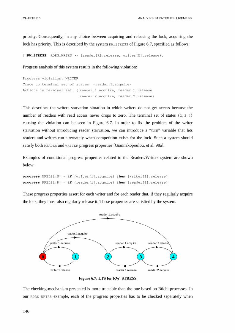
CHAPTER 6 ANALYSIS STRATEGIES: LIVENESS
146
priority. Consequently, in any choice between acquiring and releasing the lock, acquiring the
lock has priority. This is described by the systemRW_STRESSof Figure 6.7, specified as follows:
||RW_STRESS= RDRS_WRTRS >> {reader[R].release, writer[W].release}.
Progress analysis of this system results in the following violation:
Progress violation: WRITER
Trace to terminal set of states: <reader.1.acquire>
Actions in terminal set: { reader.1.acquire, reader.1.release,
reader.2.acquire, reader.2.release}
This describes the writers starvation situation in which writers do not get access because the
number of readers with read access never drops to zero. The terminal set of states {2,3,4 }
causing the violation can be seen in Figure 6.7. In order to fix the problem of the writer
starvation without introducing reader starvation, we can introduce a “turn” variable that lets
readers and writers run alternately when competition exists for the lock. Such a system should
satisfy bothREADERandWRITERprogress properties [Giannakopoulou, et al. 98a].
Examples of conditional progress properties related to the Readers/Writers system are shown
below:
progress WREL[i:W] = if {writer[i].acquire} then {writer[i].release}
progress RREL[i:R] = if {reader[i].acquire} then {reader[i].release}
These progress properties assert for each writer and for each reader that, if they regularly acquire
the lock, they must also regularly release it. These properties are satisfied by the system.
reader.1.acquire
reader.2.acquire
writer.1.acquire
writer.1.release
reader.1.acquire
reader.1.release
reader.2.release
reader.2.acquire
0 1 2 3 4
Figure 6.7: LTS for RW_STRESS
The checking-mechanism presented is more tractable than the one based on Büchi processes. In
our RDRS_WRTRSexample, each of the progress properties has to be checked separately when
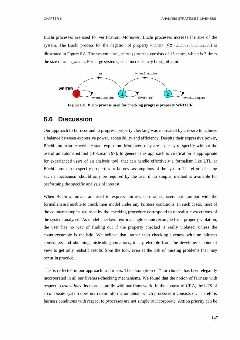
CHAPTER 6 ANALYSIS STRATEGIES: LIVENESS
147
Büchi processes are used for verification. Moreover, Büchi processes increase the size of the
system. The Büchi process for the negation of propertyWRITER (◊□¬writer.1.acquire ) is
illustrated in Figure 6.8. The systemRDRS_WRTRS||WRITERconsists of 15 states, which is 3 times
the size ofRDRS_WRTRS. For large systems, such increase may be significant.
WRITER
tau
writer.1.acquire
writer.1.acquire
@WRITER writer.1.acquire0 1 2
Figure 6.8: Büchi process used for checking progress property WRITER
6.6 Discussion
Our approach to fairness and to progress property checking was motivated by a desire to achieve
a balance between expressive power, accessibility and efficiency. Despite their expressive power,
Büchi automata exacerbate state explosion. Moreover, they are not easy to specify without the
use of an automated tool [Holzmann 97]. In general, this approach to verification is appropriate
for experienced users of an analysis tool, that can handle effectively a formalism like LTL or
Büchi automata to specify properties or fairness assumptions of the system. The effort of using
such a mechanism should only be required by the user if no simpler method is available for
performing the specific analysis of interest.
When Büchi automata are used to express fairness constraints, users not familiar with the
formalism are unable to check their model under any fairness conditions. In such cases, most of
the counterexamples returned by the checking procedure correspond to unrealistic executions of
the system analysed. As model checkers return a single counterexample for a property violation,
the user has no way of finding out if the property checked is really violated, unless the
counterexample is realistic. We believe that, rather than checking liveness with no fairness
constraints and obtaining misleading violations, it is preferable from the developer’s point of
view to get only realistic results from the tool, even at the risk of missing problems that may
occur in practice.
This is reflected in our approach to fairness. The assumption of “fair choice” has been elegantly
incorporated in all our liveness-checking mechanisms. We found that the notion of fairness with
respect totransitionsfits more naturally with our framework. In the context of CRA, the LTS of
a composite system does not retain information about which processes it consists of. Therefore,
fairness conditions with respect toprocessesare not simple to incorporate. Action priority can be

CHAPTER 6 ANALYSIS STRATEGIES: LIVENESS
148
used to increase the coverage of the checking mechanism under fair choice. The advantage of
action priority is that it is simple to model, and the LTS of the system is automatically updated
accordingly. The users can therefore easily experiment with enforcing various adverse
scheduling conditions based on their intuition about vulnerable parts of the system behaviour.
Note that action priority does not provide full control over the actions of a system. For example,
it can only be applied at the last stage of system construction with CRA, and it cannot select the
path to follow at a non-deterministic choice.
The proposed progress-checking mechanism provides a way of checking liveness in a system,
which is easily accessible by non-experts. Although less expressive than LTL and Büchi
automata, progress properties can be specified in a simple intuitive way, and can be checked on
the LTS of the system without modifying it or increasing its size. In the context of CRA, progress
properties are specified independently of the processes and composite subsystems that form a
system. Consequently, they can be applied meaningfully to a subsystem as well as to the
composite system as long as the subsystem contains the progress actions in its alphabet. A single
traversal of the LTS of a system is sufficient to check any number of progress properties.
In our framework, progress and safety checking can be combined efficiently, and checked in a
system simultaneously. Therefore, users need to revert to ALTL and Büchi automata only for
restricted classes of liveness properties. Our experience and that of others lead us to believe that
progress properties are sufficiently expressive to allow many liveness properties of interest to be
verified. For example, we have applied our technique to a large model of an Active Badge
System [Magee, et al. 97], and shown that badge commands are not acknowledged if badges
move between locations too frequently. In their work on patterns in property specifications,
[Dwyer, et al. 98] report that the most common property pattern isResponse, described in LTL as
□(a ⇒◊b) . Our progress and conditional progress schemes cover a wide range of properties that
fall in this category. For example, when□◊a holds in a system,□(a ⇒◊b) is equivalent to the
conditional progress property “progress Response = if {a} then {b} ”.
6.7 Deterministic Büchi processes
Let P be a system expressed as an LTS andf a property thatP must satisfy. Suppose thatf can be
expressed by a deterministic Büchi processB, whereB is complete and free ofτ-transitions. For
brevity, we will refer to such processes simply as deterministic Büchi processes. We have
mentioned thatP satisfiesf iff all infinite words defined by executions ofP are accepted byB.
But sinceB is deterministic, a single execution ofB is possible on any such word. Therefore,P

CHAPTER 6 ANALYSIS STRATEGIES: LIVENESS
149
satisfies f iff @B is enabled infinitely often in all executions ofP||B over α(P||B). This is
equivalent to saying that @B is enabled in every reachable cycle ofP||B. The latter reduces to
checking that the graph obtained fromP||B by removing the states where @B is enabled, is a-
cyclic (this is computationally inexpensive) [Fernandez, et al. 92a].
As B is complete, it does not affect the behaviour ofP when composed with it. This means that
multiple properties can be checked simultaneously onP if these properties are expressed as
deterministic Büchi processesB1…Bn. ThenP satisfies the properties iff∀ 1≤i≤n, @Bi is enabled
in all cycles ofP||B1||…||Bn. This can be performed by applying, for each @Bi separately, the
technique proposed by [Fernandez, et al. 92a]. After checking that the system satisfies its desired
properties, all accepting transitions are removed and the system is minimised with respect to
observational equivalence. The resulting system is observationally equivalent toP. This is easily
proven as follows: if all accepting transitions @B of a complete Büchi processB= ⟨S, A∪{ @B},
∆, q, {@B} ⟩ are removed, then the result is equivalent to the LTSB´= ⟨{ q}, A, ∆ , q⟩ where
∆´={(q, a, q) | a ∈ A}. Such an LTS is transparent to any systemP for whichαB´⊆αP.
The checking mechanism described above becomes much more efficient when the system
executes under fair choice. In that case,P satisfies the properties expressed byB1…Bn iff,
∀1≤i≤n, @Bi is enabled in all terminal sets of states ofI=P||B1||…||Bn. Therefore this check is
performed by simply computing the terminal sets of states inI. Moreover, as mentioned, fair
choice does not require the use of the RD algorithm in the context of CRA. The Büchi processes
introduced into analysis may contain internal actions of subsystems, since they can be introduced
in the compositional hierarchy.
We have to mention at this point that the developer of a system that wishes to analyse a design
needs to make a conscious choice between checking properties simultaneously or one at a time in
the system. The disadvantage of checking a single property at a time is that any change in the
system requires checking all established properties again, one by one. Admittedly, the system
state-space grows with each property included. However, if state explosion does not occur, all
safety properties and those liveness properties expressible as deterministic Büchi processes can
be checked simultaneously on a system. When no violations are detected, accepting transitions
are removed from the system, and the LTS obtained is minimised. The resulting LTS describes
the behaviour of the system, abstracted from details as required by the developer. The RMTP
case study discussed in Chapter 7 demonstrates this approach.

CHAPTER 6 ANALYSIS STRATEGIES: LIVENESS
150
6.8 General methodology
safety-property LTSs
Büchi Automata/Processes (BA/P)
deterministic BA/P
progress
ALTL
Figure 6.9: Classes of properties supported by TRACTA
We have proposed a number of methods for analysing properties of concurrent and distributed
systems. TRACTA supports a basic mechanism for checking properties expressed as Büchi
automata (or Büchi processes equivalently), but is also equipped with strategies that make this
test more efficient for subclasses of Büchi automata: safety and progress properties, and
deterministic Büchi automata (see Figure 6.9). We have also introduced the notions of fair choice
and action priority when checking liveness properties. In this section, we propose a way of
putting all these methods together into a practical approach to system analysis. We assume that a
system is described as a hierarchy of components, and that CRA is used for computing the
system behaviour. Then analysis should proceed as follows:
1. Express safety properties as property LTSs, and include them in the compositional hierarchy.
Identify, among the desired liveness properties, those that involve internal actions of
subsystems, and try to express them as deterministic Büchi automata. Include such
deterministic Büchi automata in the compositional hierarchy. Perform CRA with fair choice.
If state explosion occurs, try omitting the liveness properties, as it is more critical to check
safety first. If the system can still not be analysed, try including the properties one at a time.
2. On the graph obtained from step 1, check for deadlocks and safety property violations. If
violations are detected, debug the design based on the counterexamples obtained, and go
back to step 1. If all safety properties are satisfied, then check the liveness properties. Use

CHAPTER 6 ANALYSIS STRATEGIES: LIVENESS
151
action priority to refine the checks, if necessary. As mentioned, safety properties must be
checked before applying action priority since the latter may possibly remove erroneous
system behaviour. If violations occur, correct the design and return to step 1. If the liveness
properties are satisfied, remove all accepting transitions from the system and minimise it.
The LTS obtained describes the abstracted behaviour of the system.
3. On the graph obtained from step 2, check progress properties and apply action priority to
increase the confidence in the tests. If violations are detected, correct as appropriate and
repeat step 1. If no violations are detected and there remain liveness properties to be checked,
proceed to step 4.
4. Check liveness properties not covered by progress tests and deterministic Büchi automata.
Use Büchi automaton for the negation of the property. If the property involves internal
actions of subsystems, the automaton has to be included in the compositional hierarchy. In
that case, the behaviour of subsystems affected by the addition of a component in the
compositional hierarchy must be re-computed. Each property is then checked separately,
with the following procedure:
• First perform a test under fair choice (again, action priority can be applied). If
violations introduce changes, start again at step 1.
• If necessary, perform a test without fairness assumptions. Add fairness constraints if
appropriate. In this case CRA must be performed to the system from scratch, because it
must apply the RD algorithm. If changes need to be introduced, go to step 1.
The methodology presented reflects two main concerns in an analysis approach. Particular
emphasis needs to be placed on satisfying the safety requirements of a system, as safety
violations may have catastrophic consequences. Liveness is a desirable, though less critical,
feature. The other concern has to do with the cost of analysis. It is good practice to postpone
expensive checks towards the later stages of analysis. At these stages, systems are likely to
contain fewer violations, because the designs have been refined by earlier and possibly less
exhaustive checks.
6.9 Summary
This chapter has focused on liveness property checking. We have explained why some notion of
fairness is necessary when analysing liveness characteristics of a design. To this end, our
checking mechanisms provide a “fair choice” option, which filters out violations of liveness

CHAPTER 6 ANALYSIS STRATEGIES: LIVENESS
152
properties that do not correspond to real executions of the system analysed. Unfortunately, it
often ignores violations that may occur in practice. In order to refine the results obtained under
fair choice, we have proposed an action priority scheme for checking the system under adverse
conditions. Action priority provides a simple but effective way of examining the behaviour of a
system under adverse scheduling conditions. To improve this control, we plan to investigate the
use of both relative and dynamic action priorities. The assumption of fair choice simplifies the
checking mechanism for liveness properties in a system, particularly in the context of CRA.
We have proposed a method for checking a specific class of liveness properties, which we call
progress. Progress properties are simple to specify and efficient to check. A significant advantage
of the progress checking mechanism presented is that it does not increase the state space of the
system. Even though progress properties do not supplant the need for general LTL model
checking, they are sufficiently expressive to cover many liveness properties of interest.
Finally, we have provided mechanisms for checking multiple liveness properties simultaneously
when these can be expressed as deterministic Büchi automata. We have concluded by proposing
a methodology that puts together all verification techniques supported by TRACTA, i.e. the basic
checking mechanism presented in Chapter 4, as well as the analysis strategies for safety and
liveness properties described in Chapters 5 and 6, respectively. This methodology provides a
number of steps which developers are advised to follow when using TRACTA for system analysis.

153
Implementation & Evaluation 77.1 ENVIRONMENT 153
7.2 TOOL IMPLEMENTATION 155
7.3 CASE STUDY: A RELIABLE MULTICAST TRANSPORT PROTOCOL 160
7.4 EVALUATION AND DISCUSSION 175
7.5 SUMMARY 178
The TRACTA approach has been motivated by the need to introduce analysis as an integrated part
of system development. In an integrated environment, analysis and modelling should go hand in
hand with design so as to permit distributed systems designers to explore and check their designs
incrementally and naturally. As discussed in previous chapters, TRACTA attempts to address this
requirement by performing analysis based on the software architecture of the system.
In this chapter, we discuss how the integration advocated by our methods is reflected in our tools.
We describe the construction of our current analysis tool, as well as the way it has been
introduced in our environment for the development of distributed systems. Finally, we use our
methods and tools to check a reliable multicast transport protocol (RMTP). The RMTP is a non-
trivial case study with which we evaluate the overall practicality and efficiency of our approach.
7.1 Environment
The Software Architect’s Assistant (SAA) [Ng, et al. 96] plays the main role in the integration of
our methods. The SAA is a visual environment for the design and development of distributed
programs using Darwin architectural descriptions. Facilities provided include the display of
multiple integrated graphical and textual views, a flexible mechanism for recording design
information and the automatic generation of program code and formatted reports from design
diagrams. The architecture of a system is used by the Darwin compiler to generate a system
instance. The hierarchical structure of a system instance can then be utilised for analysis.
The SAA is currently being re-implemented in Java to aid portability and interoperability. The
new version of the SAA additionally generates FSP expressions corresponding to the system
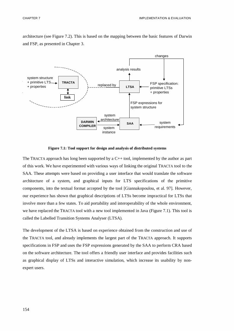
CHAPTER 7 IMPLEMENTATION & EVALUATION
154
architecture (see Figure 7.2). This is based on the mapping between the basic features of Darwin
and FSP, as presented in Chapter 3.
systemrequirements
SAADARWINCOMPILER
systemarchitecture
systeminstance
LTSAFSP specification:primitive LTSs+ properties
FSP expressions forsystem structure
replaced by
analysis results
changes
TRACTA
link
system structure+ primitive LTS+ properties
Figure 7.1: Tool support for design and analysis of distributed systems
The TRACTA approach has long been supported by a C++ tool, implemented by the author as part
of this work. We have experimented with various ways of linking the original TRACTA tool to the
SAA. These attempts were based on providing a user interface that would translate the software
architecture of a system, and graphical inputs for LTS specifications of the primitive
components, into the textual format accepted by the tool [Giannakopoulou, et al. 97]. However,
our experience has shown that graphical descriptions of LTSs become impractical for LTSs that
involve more than a few states. To aid portability and interoperability of the whole environment,
we have replaced the TRACTA tool with a new tool implemented in Java (Figure 7.1). This tool is
called the Labelled Transition Systems Analyser (LTSA).
The development of the LTSA is based on experience obtained from the construction and use of
the TRACTA tool, and already implements the largest part of the TRACTA approach. It supports
specifications in FSP and uses the FSP expressions generated by the SAA to perform CRA based
on the software architecture. The tool offers a friendly user interface and provides facilities such
as graphical display of LTSs and interactive simulation, which increase its usability by non-
expert users.

CHAPTER 7 IMPLEMENTATION & EVALUATION
155
7.2 Tool implementation
In this section, we describe the main analysis functions of the LTSA and TRACTA tools and
concentrate on the algorithms that implement these functions. Our discussion focuses on those
aspects of the tools that are implementation-independent, and can guide in the extension of
existing tools towards supporting the TRACTA approach. Besides the features that implement the
core of the approach, we also discuss the user-interface and additional features that our tools
provide, which significantly contribute to their usability. Note that, as Büchi processes and LTSs
are treated uniformly by our tools, they are both referred to as LTSs in this chapter.
Figure 7.2: The Software Architect’s Assistant (SAA)
7.2.1 System construction
In the following, we describe the functions of our tools related to the computation of system
behaviour.
Compile. Generates an LTS for each primitive process specified. Some of the specifications may
correspond to safety or liveness properties, or to user-specified interfaces. These must be
automatically transformed for analysis as required by the TRACTA approach. More specifically,
safety-property and interface LTSs are turned into their image processes (Chapter 5), and Büchi
automata are translated into their corresponding Büchi processes (Chapter 4).
Compose.Computes the LTS of a composite component from those of its sub-components. The
LTS returned can be analysed or further composed. The composition algorithm is

CHAPTER 7 IMPLEMENTATION & EVALUATION
156
straightforward; a standard one can be found in [Holzmann 91]. An option of this function is for
the sub-components to be minimised before composition. In the TRACTA tool, the user performs
each step of CRA explicitly, by calling this function for each composite component in the
system. The LTSs of intermediate systems are stored after composition, and are used for
computing higher level components. In this way, the user selects for each subsystem whether the
minimisation option is set during composition.
The LTSA takes a different approach. The user selects a target from the list of composite
expressions in the specifications. The LTSs of composite components that have been computed
are not stored after composition. The LTS for a target is computed with CRA from the LTSs of
primitive components, based on the sub-tree rooted at the target in the compositional hierarchy.
The option “minimise during composition” is then a global option during this computation, i.e. it
is set for all or none of the compositions performed during the computation of the target
behaviour. The advantage of the LTSA is that the user does not perform each step of CRA
explicitly. While maintaining this advantage, we plan to offer the flexibility of selecting which
components of a target system are to be minimised during CRA.
Record Divergence.Applies the RD or optimised RD algorithm to an LTS, as described in
Sections 4.5.1 and 4.6. As mentioned, this is useful when fair choice is not a desirable
assumption in the model of a system, and the system is minimised with respect to weak
equivalence. The RD algorithms rely on the computation of strongly-connected components in a
state-graph, for which the TRACTA tool implements the algorithm proposed by [Aho, et al. 74].
The complexity of the algorithm is linear in the size of the graph. The LTSA tool does not yet
support this function.
Minimise. Minimises a given LTSL with respect to Milner’s weak semantic equivalence [Milner
89]. Minimising an LTSP = ⟨S, A, ∆, q0⟩ with respect to weak equivalence is performed by first
transformingP into P´ = ⟨S, A, ∆ , q0⟩ and subsequently minimisingP´ with respect to strong
equivalence, where∆´ = {(p, a, q) | p⇒a q in P, a∈A} ∪{( p, τ, p) | p∈ S}. This transformation of
the LTS involves the computation of the reflexive transitive closure→ *τ of its τ-relation, and
subsequently, the computation of the relational composition (Rτ · Ra · Rτ) ∀a∈αP, where
→= ττ
*R and →= aaR . The transformation takes time that is cubic in the number of nodes
in the graph.
In general, the time complexity of performing minimisation modulo strong equivalence isO(mn)
for an LTS with m transitions andn states [Kanellakis and Smolka 90]. However, a more

CHAPTER 7 IMPLEMENTATION & EVALUATION
157
efficient algorithm has been presented by [Fernandez 90]. This algorithm is based on the
established relationship between checking strong equivalence and the relational coarsest partition
problem. The latter can be solved in timeO(mlogn) as proven by [Paige and Tarjan 87]. The
Paige and Tarjan algorithm applies to state transition systems where transitions are not labelled.
Fernandez has adapted this algorithm to handle LTSs.
The TRACTA tool implements the Fernandez algorithm, whereas the LTSA implements a less
efficient but much simpler algorithm described by [Holzmann 91]. We have found that in many
cases, the simplicity of the latter algorithm and of the data structures it uses make it faster than
the former. Moreover, experience with various case studies has shown that the complexity of
computing weak equivalence is often dominated by the initial transformation of the LTS. In
general, there is not enough evidence to suggest that the algorithm by Paige and Tarjan is
appreciably faster in practice [Cleaveland, et al. 93b]. In order to gain more experience on the
relative performance of the two algorithms, we intend to add the Fernandez algorithm in the
LTSA tool. As minimisation takes up most of the computation time during CRA, the issue is
further discussed later in this chapter.
7.2.2 System analysis
In the following, we describe the functions of our tools related to system analysis.
Check safety. Detects deadlocks and safety property violations on an LTS. Deadlocks are
identified as states with no outgoing transitions. Safety property violations are detected when the
error-stateπ is reachable in the LTS. When a design contains errors, a counterexample is
returned to help with debugging. A counterexample describes a trace of the system leading to
deadlock, or to stateπ. To generate traces to specific states of an LTS, our tools traverse the LTS
in a breadth-first way. This guarantees the shortest possible counterexamples.
As mentioned in Chapter 5, when multiple safety properties are simultaneously analysed, the tool
can detect safety violations but it cannot distinguish which property is violated. In fact, during
composition, the LTSA informs which subsystems contribute to the existence of stateπ in the
composite system. If the counterexample returned does not identify a property, then it may be
used to track the violation in more primitive components of the compositional hierarchy.
Check liveness.Performs liveness property checks on an LTS. Progress checks are performed as
described in Chapter 6, and only under fair choice. Fair choice is an option of the LTSA tool
when checking liveness properties expressed as Büchi automata. The LTSA tool currently

CHAPTER 7 IMPLEMENTATION & EVALUATION
158
supports the standard model-checking mechanism, where the automaton for the negation of the
property is used. The algorithm proposed in Section 6.7 for deterministic Büchi automata is to be
added soon.
When a liveness property violation is detected under fair choice, the trace to a violating terminal
set of states is returned, together with the actions enabled in the terminal set. As for the case of
safety properties, theshortestpossible trace to the terminal set is returned. When fair choice is
not assumed, the trace to a violating strongly-connected component is returned instead, together
with a cyclic trace within the component.
7.2.3 Interface and additional features
To allow the user to assess and compare various approaches to system analysis, our tools provide
the following information:
• time required for LTS composition or LTS minimisation;
• sizes (#states and #transitions) of LTSs obtained with composition or minimisation.
STOPBUTTON
TARGET
FSPWINDOW
OUTPUTWINDOW
Figure 7.3: Interface of the LTSA tool

CHAPTER 7 IMPLEMENTATION & EVALUATION
159
The interface of the LTSA tool is illustrated in Figure 7.3. The LTSA window contains four
objects apart from the menu-bar:
1. The FSP window is used to enter the FSP specification of a system.
2. The Output window contains the results of analysis, counterexamples, timing results, as well
as error messages generated by the FSP parser.
3. The target choice box is used to select the process to be analysed, among the composite
processes in the specification.
4. The Stop button is highlighted when the LTSA is performing a computation that could
potentially take a long time. Clicking on the Stop button will abort the activity.
The functions supported by the LTSA include: creation, saving and opening of FSP specification
files; parsing of FSP expressions; checking of a target LTS with respect to safety, liveness and
progress; interactive simulation of a target process; composition and minimisation of a target
process; graphical or textual display of LTSs (most of the LTS diagrams included in this thesis
have been created with the LTSA tool).
The functions of the LTSA are invoked from the menu-bar at the top of the LTSA window. From
the Option menu, minimisation during composition and fair choice can be enabled or disabled.
The Template menu provides a set of templates for ALTL properties that are frequently
encountered. Selecting a template will insert the FSP description of the corresponding Büchi
automaton for the negation of the property. The user may then rename the actions involved in the
template to match them with actions of a system.
A very useful function of the LTSA is the interactive simulation of any target process in a
specification. This consists of a user-controlled animation of the process. During animation, the
LTSA does not first compute the LTS of the target, when this target is a composite process.
Rather, it uses the LTSs of its components to compute just the state in which the target transits,
when the action selected by the user is performed. As a result, animation does not suffer from
state explosion; it can be used to experiment with the behaviour of large systems even if they
cannot be checked exhaustively.
With each animation step, the LTSA highlights on the graphical display of the component LTSs,
the transition(s) performed by these LTSs, as well as the states in which they transit. The set of
actions controlled by the user is by default the alphabet of the target composite process, before

CHAPTER 7 IMPLEMENTATION & EVALUATION
160
any hiding is applied to it. In essence, animation simulates the joint behaviour of a group of LTSs
that make up a composite component. The actions controlled by the user may be reduced by
explicitly including a process MENU in the target composition. For example, the specification of
the toss of a coin is animated as illustrated in Figure 7.4. In the animator window, ticked boxes
indicate enabled actions.
COIN
toss
toss
heads
tails
0 1 2
COIN = (toss -> heads -> COIN |toss -> tails -> COIN).
MENU = (toss -> MENU).
Figure 7.4: Animation of the coin tossing example
7.3 Case study: a reliable multicast transport protocol
In this section, we illustrate our technique with a non-trivial case study, which shows how fast
the size of a system consisting of several components may explode, even when these components
are small in size. In this example, the TRACTA approach has been successfully used to both
considerably reduce the size of the system, but also to check properties of interest.
7.3.1 The protocol
The Reliable Multicast Transport Protocol (RMTP) [Lin, et al. 96] is designed for applications
that cannot tolerate data loss. It provides sequenced, loss-less delivery of data from a sender to a
group of receivers, at the expense of delay. Reliability is achieved by a periodic transmission of
acknowledgements by the receivers and a selective retransmission mechanism by the sender. For
scalability, receivers are grouped into a hierarchy of local regions, with aDesignated Receiver
(DR) in each of those regions. Receivers in each local region send their acknowledgements to the
corresponding DR, DRs send their acknowledgements to the higher level DRs or to the sender
(Figure 7.5), thereby avoiding the acknowledgement implosion problem. DRs cache received
data and are in charge of retransmissions within their local regions, thus decreasing end-to-end
latency. The termAcknowledgement Processor(AP) is used to denote either a designated

CHAPTER 7 IMPLEMENTATION & EVALUATION
161
receiver or the sender, when referring to them as entities that receive and process
acknowledgements. Receivers that are not designated receivers are referred to asordinary
receivers.
REC_B
Ack
Router
OrdinaryReceiver
SENDER
DesignatedReceiver
DES_REC_B
DES_REC_A
REC_C REC_A REC_D
Sender
Figure 7.5: A multicast tree of receivers
To cater for situations where designated receivers may fail, receivers use a mechanism to
dynamically select the nearest operational AP in the multicast tree. This is the part of the RMTP
protocol on which this case study focuses. In the RMTP, dynamic selection of APs is achieved
by the use of a special packet, called theSEND_ACK_TO_ME packet. The sender and all DRs
periodically advertise themselves by multicastingSEND_ACK_TO_MEpackets along their sub-trees.
These packets are tagged with the same initialTIME_TO_LIVE values. Routers decrement the
TIME_TO_LIVE value when forwarding packets. Therefore, a largerTIME_TO_LIVE value indicates a
closer proximity in the multicast tree. On receipt of aSEND_ACK_TO_ME packet, a receiver
compares theTIME_TO_LIVE value associated with the incoming packet, with that associated with
the AP currently selected. The receiver switches to a new AP if the incoming packet has a larger
TIME_TO_LIVE value. When a receiver fails to receive a newSEND_ACK_TO_ME packet from the
currently selected AP after a certain period of time, it assumes failure of the AP and initiates a
new selection round.
7.3.2 Structure of the RMTP
In the RMTP case study, both ordinary and designated receivers can be further decomposed into
processes of the following types (see Figure 7.6 and Figure 7.7):RECEIVER(N) , CHANNEL(N), and
TIMER for ordinary receivers, andDES_RECEIVER(N), DES_CHANNEL(N)andTIMER for designated
receivers. Processes of typeRECEIVER(N) and DES_RECEIVER(N) implement the main
functionality of the components, i.e. the dynamic selection of acknowledgement processor.
Processes of typeCHANNEL(N)andDES_CHANNEL(N)implement unreliable channels that may lose
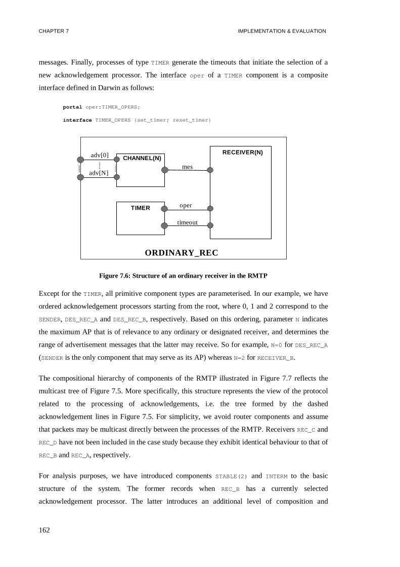
CHAPTER 7 IMPLEMENTATION & EVALUATION
162
messages. Finally, processes of typeTIMER generate the timeouts that initiate the selection of a
new acknowledgement processor. The interfaceoper of a TIMER component is a composite
interface defined in Darwin as follows:
portal oper:TIMER_OPERS;
interface TIMER_OPERS {set_timer; reset_timer}
CHANNEL(N)
TIMER
RECEIVER(N)
mes
oper
ORDINARY_REC
timeout
adv[0]
adv[N]
Figure 7.6: Structure of an ordinary receiver in the RMTP
Except for theTIMER, all primitive component types are parameterised. In our example, we have
ordered acknowledgement processors starting from the root, where 0, 1 and 2 correspond to the
SENDER, DES_REC_AandDES_REC_B, respectively. Based on this ordering, parameterN indicates
the maximum AP that is of relevance to any ordinary or designated receiver, and determines the
range of advertisement messages that the latter may receive. So for example,N=0 for DES_REC_A
(SENDERis the only component that may serve as its AP) whereasN=2 for RECEIVER_B.
The compositional hierarchy of components of the RMTP illustrated in Figure 7.7 reflects the
multicast tree of Figure 7.5. More specifically, this structure represents the view of the protocol
related to the processing of acknowledgements, i.e. the tree formed by the dashed
acknowledgement lines in Figure 7.5. For simplicity, we avoid router components and assume
that packets may be multicast directly between the processes of the RMTP. ReceiversREC_Cand
REC_Dhave not been included in the case study because they exhibit identical behaviour to that of
REC_BandREC_A, respectively.
For analysis purposes, we have introduced componentsSTABLE(2) and INTERM to the basic
structure of the system. The former records whenREC_B has a currently selected
acknowledgement processor. The latter introduces an additional level of composition and

CHAPTER 7 IMPLEMENTATION & EVALUATION
163
minimisation in the expression corresponding toLOC_REG_2. Finally, all grey-coloured
components in Figure 7.7 represent properties for analysis – these are discussed later on.
TIMER
DES_CHANNEL(0)DES_RECEIVER(0)
DES_REC_A
LOC_REG2 SENDER
REC_A
LOC_REG1
DES_CHANNEL(1)
DES_REC_B
DES_RECEIVER(1)
TIMER
AP_SELECT
INTERM
RECEIVER(2) CHANNEL(2)
TIMER
REC_B
LIV_REC_B
STABLE(2)
RECEIVER(1) CHANNEL(1)
TIMERLIV_REC_A
SAF_LC_REG1´
Figure 7.7: Compositional hierarchy for the RMTP
7.3.3 Modelling component behaviour for the RMTP
In order to avoid extensive renaming and to simplify the presentation of our case study, we do
not give instance names to components. Action labels are thus not prefixed with instance names,
and have been chosen carefully to avoid unwanted synchronisation during composition.
Ordinary receivers
Ordinary receivers are decomposed into processesRECEIVER(N) , CHANNEL(N), and TIMER (see
Figure 7.6), specified as follows:
TIMER = COUNT_DOWN, // initially sender is selected, so timer counts down
START = ( oper.set_timer -> COUNT_DOWN),
COUNT_DOWN = ( count_down -> COUNT_DOWN
| oper.reset_timer -> COUNT_DOWN
| timeout -> START)
@ {oper, timeout}. // external interface

CHAPTER 7 IMPLEMENTATION & EVALUATION
164
CHANNEL (N=1) = ( adv[i:0..N] -> mes[i] -> CHANNEL // default value of N is 1
| adv[i:0..N] -> lose -> CHANNEL)
@ {adv, mes}.
RECEIVER (N=1) = AP[0], // initially SENDER is the selected AP
AP[i:0..N] = ( mes[i]-> oper.reset_timer -> AP[i] // current AP is i
| timeout -> NO_AP
| when (i>0) mes[k:0..i-1] -> AP[i]
| when (i<N) mes[k:i+1..N] -> SELECT[k]),
NO_AP = ( mes[i:0..N]-> SELECT[i]), // no AP currently selected
SELECT[i:0..N] = ( sel[i] -> SET_TIMER[i]),
SET_TIMER[i:0..N] = (oper.set_timer -> AP[i]).
//sel actions not hidden yet - needed for recording stability of receivers
Process typeTIMER behaves as follows. Withoper.set_timer , the timer transits from the idle
state (START) to state COUNT_DOWN(auxiliary processes may be viewed as states). At state
COUNT_DOWN, the timer counts down to zero after which it issues a timeout event. The operation
oper.reset_timer resets the timer to the initial value, where it starts counting down again. As
illustrated in Figure 7.6, the interface of the counter consists of the operations that it offers, and
the timeout event that it issues (@{oper, timeout} ).
ProcessCHANNEL(N) implements a lossy channel of capacity one. We have avoided adding
buffers in our example as they can significantly complicate and increase the size of the case
study. Buffers are not necessary because the channels can always deal with the messages they
contain and are then ready to receive new messages. As a result, the capacity of one does not
introduce any deadlocks. As mentioned in Chapter 3, such channels are specified as non-
deterministic processes. Here, the channel may receive advertisements from the relevant range of
APs (i:0..N ). On receipt of each message, it non-deterministically commits to transmit it
(mes[i] ), or to lose it (lose ). The interface of the channel consists of the actions in its alphabet
prefixed withadv andmes.
Process typeRECEIVER(N) implements the dynamic selection of AP. In the RMTP, all receivers
initially select the sender as their AP, which is reflected by the fact that the process starts at state
AP[0] (0 corresponds to the sender). When the receiver is in stateAP[i] (“ i ” is the currently
selected AP), then it may choose one of the following alternatives:
• on receipt of a messagemes[i] through its channel, it knows that the current AP is
operational, and therefore resets the timer to its initial value;

CHAPTER 7 IMPLEMENTATION & EVALUATION
165
• if a timeout occurs, it assumes that the current AP is not alive, and transits to state
NO_AP;
• on receipt of an advertisement messagemes[k] corresponding to a nearer AP (i.e.k>i ), it
decides to selectk as its AP and transits to stateSELECT[k] . Otherwise, ifk<i , mes[k] is
ignored.
When in stateNO_AP, the receiver selects the first AP from which it receives an advertisement
message. After selecting an AP, the receiver also sets the timer. In this way, if no advertisement
is received within the set timeout period, the receiver assumes that the AP is no longer
operational.
As mentioned, processSTABLE(N) is introduced for analysis purposes. We say that a receiver is
stablewhen it is at a state where it has a currently selected AP. ProcessSTABLE(N) monitors the
stability of the receiver with which it is associated. Stability is reflected by the fact that process
STABLE is able to perform actionrec_stable . Initially, all receivers are stable since they choose
the sender as AP. Action timeout leads to the unstable state from which stability is reached again
with the selection of a new AP. We have expressed the behaviour of this process in FSP as
follows:
STABLE (N=1) =( rec_stable -> STABLE
| sel[i:0..N] -> STABLE
| timeout -> UNSTABLE),
UNSTABLE= (sel[i:0..N] -> STABLE).
The ordinary receivers included in our case study areREC_AandREC_B. From Figure 7.5, we can
see thatN=1 for REC_A, and N=2 for REC_B. We have also introduced processSTABLE(2) for
REC_B, thus concluding in the following specifications forREC_A and REC_B, based on the
structural description of Figure 7.6:
|| REC_B = ( RECEIVER(2) || TIMER || CHANNEL(2) || STABLE(2))
@ {adv, rec_stable}.
|| REC_A = (RECEIVER(1) || TIMER || CHANNEL(1)) @ {adv}.
Note that actionrec_stable is part of the external interface ofREC_B, because we wish this
action to be visible at the global system. In fact, with CRA we attempt to obtain an abstracted
view of the RMTP protocol, where only failures of designated receivers, and their impact on the
stability of REC_Bare observable. We have decided to check the stability ofREC_B, because it is

CHAPTER 7 IMPLEMENTATION & EVALUATION
166
the ordinary receiver at the lowest level of the multicast tree, and it is therefore affected by the
failures of both designated receiversDES_REC_AandDES_REC_B.
Designated receivers
Designated receivers behave like ordinary receivers, except that they may fail and advertise
themselves. In our case study, we do not hide actions related to the failure of designated
receivers. Although these actions are not part of the external interface, we want them to be
visible at the global system level. However, we need to rename them appropriately, so that
DES_REC_AandDES_REC_Bdo not synchronise on actionfail . The behaviour specifications are
as follows:
DES_RECEIVER (N=1) = AP[0],
AP[i:0..N] = ( mes[i]-> oper.reset_timer -> AP[i]
| timeout -> NO_AP
| when (i>0) mes[k:0..i-1] -> AP[i]
| when (i<N) mes[k:i+1..N] -> SELECT[k]
| adv[N+1] -> AP[i] // the DR advertises itself
| fail -> STOP),
NO_AP = ( mes[i:0..N]-> SELECT[i]
| adv[N+1] -> NO_AP // the DR advertises itself
| fail -> STOP),
SELECT[i:0..N] = ( sel[i] -> SET_TIMER[i]
| fail -> STOP),
SET_TIMER[i:0..N] = ( oper.set_timer -> AP[i]
| fail -> STOP).
DES_CHANNEL (N=1) = ( adv[i:0..N] -> mes[i] -> DES_CHANNEL
| adv[i:0..N] -> lose -> DES_CHANNEL
| fail -> FAILED_REC),
FAILED_REC = ( adv[i:0..N] -> FAILED_REC)
@ {adv, mes, fail}.
|| DES_REC_A = (DES_RECEIVER(0) || TIMER || DES_CHANNEL(0))
/ {dra_fail/fail} @ {adv, dra_fail}.
|| DES_REC_B = (DES_RECEIVER(1) || TIMER || DES_CHANNEL(1))
/ {drb_fail/fail} @ {adv, drb_fail}.
Note that the channel of a designated receiver needs to record the fact that the receiver has failed
(the channel transits into stateFAILED_REC), in which case the channel keeps consuming
advertisement messages received but no longer forwards them to theDES_RECEIVERprocess.

CHAPTER 7 IMPLEMENTATION & EVALUATION
167
Remaining components of the RMTP
We have not modelled failure for ordinary receivers and the sender. If the sender fails, the
multicast session is cancelled, in which case the RMTP does not need to fulfil its objectives.
Properties of ordinary receivers are not expected to hold when these receivers fail. Moreover,
failures of ordinary receivers do not affect the behaviour of their environment, and may therefore
be ignored.
Based on the compositional hierarchy of Figure 7.7, the remaining components of the RMTP are
expressed as follows:
|| LOC_REG1 = (REC_B || DES_REC_B) \ {adv[2] }.
|| INTERM = (REC_A || DES_REC_A).
|| LOC_REG2 = (LOC_REG1 || INTERM) \ {adv[1]}.
SENDER= (adv[0] -> SENDER).
|| AP_SELECT = (LOC_REG2 || SENDER) \ {adv[0]}.
7.3.4 Property specification
One desirable characteristic of the RMTP is that failed designated receivers should not be
selected as APs. To check this, we introduce the property illustrated in Figure 7.8. Property
SAF_LC_REG1refers to componentLOC_REG1and is included in the compositional hierarchy as
depicted in Figure 7.7.SAF_LC_REG1states that subsequently to the failure ofDES_REC_B, REC_B
(the only receiver in its sub-tree) does not selectDES_REC_Bas its AP. In fact, the property
allows REC_Bto selectDES_REC_Bat most once after the failure of the latter; it thus covers the
case whereDES_REC_Bfails immediately afterREC_B receives an advertisement from it, and
beforeREC_Bselects it as its AP.
A liveness property expected from the dynamic selection mechanism is that upon failure of a
designated receiver, all receivers in its sub-tree eventually select a different acknowledgement
processor. For componentREC_A this property reduces toLIV_RECA, which checks that if
DES_REC_Afails (dra_fail ), then REC_A is eventually able to select theSENDERas its AP
(sel[0] ). In ALTL, LIV_RECA is expressed as□(dra_fail ⇒ ◊sel[0] ).

CHAPTER 7 IMPLEMENTATION & EVALUATION
168
SAF_LC_REG1
recb_sel.2
drb_fail recb_sel.2
drb_fail
recb_sel.2drb_fail
-1 0 1 2
property SAF_LC_REG1 = ( recb_sel[2] -> SAF_LC_REG1
| drb_fail -> recb_sel[2]-> STOP).
Figure 7.8: Safety property for the RMTP
Note thatLIV_RECA requires the eventual occurrence of actionsel[0] even if DES_REC_Ais not
the currently selected AP ofREC_Awhen actiondra_fail occurs. This is because in this case
study, analysis is based on the assumption of fair choice (see Chapter 6). According to this, no
matter which is the currently selected AP, timeout expiration eventually happens and initiates a
new round of AP selection. When the AP is operational, such timeout expirations reflect a delay
in the receipt of advertisement messages sent from it. For the case ofREC_A, if a timeout occurs
after the failure ofDES_REC_A, thensel[0] must eventually happen. ThereforeLIV_RECA needs
to be satisfied by our model of the RMTP. A more complicated property could have been used to
express that “after the failure of the currently selected AP, a new AP is eventually selected” but
propertyLIV_RECA is preferred for simplicity.
Another liveness property that we wish to check isLIV_RECB. This property refers toREC_Band
states that it is eventually the case thatREC_BselectsDES_REC_Bto be its AP (sel[2] ). In ALTL,
the property is expressed as (◊sel[2] ). We thereby wish to check that, although initially all
receivers in the system start with theSENDERas their AP, each one eventually selects the one
nearest to it in the multicast tree.
Both liveness properties discussed can be expressed as deterministic Büchi automata. Therefore,
as described in Chapter 6, they can be checked simultaneously with other properties. We
therefore introduce the Büchi automata that correspond to the properties rather than to their
negations (see Figure 7.9).

CHAPTER 7 IMPLEMENTATION & EVALUATION
169
LIV_RECA
sel.0
dra_fail
@LIV_RECA
sel.0
dra_fail0 1
LIV_RECBsel.2
sel.2@LIV_RECB
0 1
LIV_RECA = ACC,
ACC @ = (sel[0] -> ACC | dra_fail -> SEL_NEW), // accepting state
SEL_NEW = (dra_fail -> SEL_NEW | sel[0] -> ACC).
LIV_RECB = (sel[2] -> ACC),
ACC @ = (sel[2] -> ACC).
Figure 7.9: Liveness properties for the RMTP
In order to check propertySAF_LC_REG1of LOC_REG_1, the local actionsel[2] of REC_B is
renamed torecb_sel[2] and may only be hidden after computingLOC_REG_1. As properties
LIV_RECA andLIV_RECB are composed intoREC_AandREC_Brespectively, they can observe the
local actions denoting the selection of AP. The FSP specifications of the components that are
affected by the introduction of properties in the RMTP are described below (see also Figure 7.7):
|| REC_A = ( RECEIVER(1) || TIMER || CHANNEL(1) || LIV_RECA)
\ {mes, oper, timeout, sel}.
|| REC_B = ( RECEIVER(2) || TIMER || CHANNEL(2) || STABLE(2) || LIV_RECB)
/ {recb_sel[2]/sel[2]}
\ {mes, oper, timeout, sel}.
|| LOC_REG1 = ( REC_B || DES_REC_B || SAF_LC_REG1)
\ {adv[2], recb_sel}.
In the above specifications, hiding of actions is performed with the restriction operator “\”. The
LTSA tool does not currently allow accepting actions in interface sets, so using restriction avoids
hiding such actions.
7.3.5 Checking the RMTP protocol
We have used the LTSA tool to analyse the model of the RMTP protocol described in the
previous sections. Analysis has increased our understanding of the system, and has helped us
uncover subtle errors in our design.
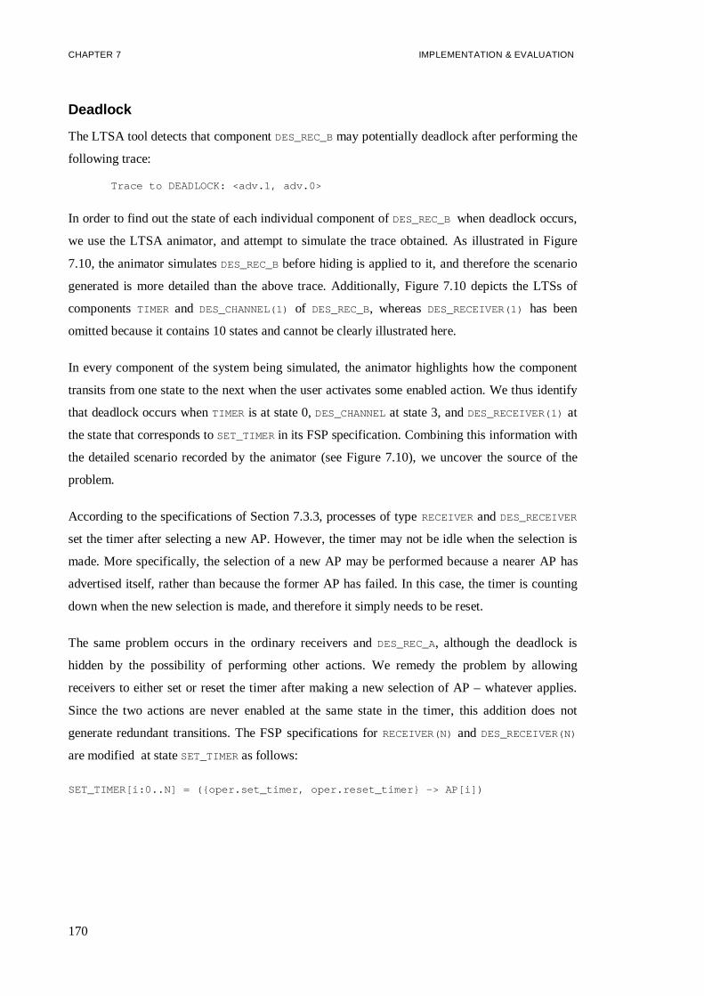
CHAPTER 7 IMPLEMENTATION & EVALUATION
170
Deadlock
The LTSA tool detects that componentDES_REC_Bmay potentially deadlock after performing the
following trace:
Trace to DEADLOCK: <adv.1, adv.0>
In order to find out the state of each individual component ofDES_REC_Bwhen deadlock occurs,
we use the LTSA animator, and attempt to simulate the trace obtained. As illustrated in Figure
7.10, the animator simulatesDES_REC_Bbefore hiding is applied to it, and therefore the scenario
generated is more detailed than the above trace. Additionally, Figure 7.10 depicts the LTSs of
componentsTIMER and DES_CHANNEL(1) of DES_REC_B, whereasDES_RECEIVER(1) has been
omitted because it contains 10 states and cannot be clearly illustrated here.
In every component of the system being simulated, the animator highlights how the component
transits from one state to the next when the user activates some enabled action. We thus identify
that deadlock occurs whenTIMER is at state 0,DES_CHANNELat state 3, andDES_RECEIVER(1) at
the state that corresponds toSET_TIMER in its FSP specification. Combining this information with
the detailed scenario recorded by the animator (see Figure 7.10), we uncover the source of the
problem.
According to the specifications of Section 7.3.3, processes of typeRECEIVERandDES_RECEIVER
set the timer after selecting a new AP. However, the timer may not be idle when the selection is
made. More specifically, the selection of a new AP may be performed because a nearer AP has
advertised itself, rather than because the former AP has failed. In this case, the timer is counting
down when the new selection is made, and therefore it simply needs to be reset.
The same problem occurs in the ordinary receivers andDES_REC_A, although the deadlock is
hidden by the possibility of performing other actions. We remedy the problem by allowing
receivers to either set or reset the timer after making a new selection of AP – whatever applies.
Since the two actions are never enabled at the same state in the timer, this addition does not
generate redundant transitions. The FSP specifications forRECEIVER(N) and DES_RECEIVER(N)
are modified at stateSET_TIMERas follows:
SET_TIMER[i:0..N] = ({oper.set_timer, oper.reset_timer} -> AP[i])

CHAPTER 7 IMPLEMENTATION & EVALUATION
171
Figure 7.10: Animating DES_REC_Bfor deadlock scenario
Safety and liveness properties
SubsystemLOC_REG1violates propertySAF_LC_REG1because theπ state is reachable in its LTS.
This violation is not remedied in the system because theπ state is also reachable inAP_SELECT.
To find out how the violation may occur, we focus on the behaviour of subsystemLOC_REG1.
When checking if the LTS ofLOC_REG1satisfies its safety property, the LTSA returns the
following counterexample trace:<drb_fail> . Unfortunately, due to action hiding, this trace is
not informative enough. To obtain a more detailed trace, we analyseLOC_REG1before hiding the
actions that are not in its interface, i.e.
|| LOC_REG1 = (REC_B || DES_REC_B || SAF_LC_REG1).
The following counterexample is then obtained:<adv.2, adv.2, drb_fail, recb_sel.2,
recb_sel.2> . This trace shows thatSAF_LC_REG1 is violated whenDES_REC_B, prior to its
failure, broadcasts two advertisements along its sub-tree. Sincerecb_sel.2 can occur twice, we
conclude that withinREC_B, CHANNEL(2) must have transmitted both advertisements to
RECEIVER(2) . We can thereby construct the following scenario that shows in detail how

CHAPTER 7 IMPLEMENTATION & EVALUATION
172
SAF_LC_REG1may be violated.CHANNEL(2) receives an advertisement fromDES_REC_B(adv.2 ),
transmits it toRECEIVER(2) , and then receives another advertisement fromDES_REC_B(adv.2 ),
after which DES_REC_B fails (drb_fail ). RECEIVER(2) selects DES_REC_B as its AP
(recb_sel.2 ). Subsequently a timeout occurs, which initiates the selection mechanism of
RECEIVER(2) . CHANNEL(2) still contains the second advertisement, which it now transmits to
RECEIVER(2) . As a resultRECEIVER(2) performs the secondrecb_sel.2 .
This violation represents a typical situation in distributed systems. In an asynchronous
environment, channels need to be equipped with substantial buffers. Consequently, nodes of the
system may be receiving old messages from a failed node, thus getting the impression that the
node is still alive. In such situations, propertySAF_LC_REG1would need to be turned into a
property stating that: “subsequently to the failure ofDES_REC_B, it is eventually the case that
REC_B never again selectsDES_REC_B as its acknowledgement processor”, or, in ALTL:
□(drb_fail ⇒ ◊□¬recb_sel[2] ).
In our simplified case study the channel has capacity one. It can therefore store at most one
advertisement fromDES_REC_Bafter the latter fails. However,drb_fail may occur in between
actionsmes[2] andsel[2] of RECEIVER(2) (see Section 7.3.4). We conclude thatSAF_LC_REG1
must allowrecb_sel[2] to occur at most twice subsequent todrb_fail :
property SAF_LC_REG1 = ( recb_sel[2] -> SAF_LC_REG1
| drb_fail -> recb_sel[2]-> recb_sel[2] -> STOP).
This modification removes the violation from the system analysed.
We check liveness properties of the RMTP under fair choice. Since the properties are expressed
as deterministic Büchi automata, a propertyP is violated by a systemSys iff Syscontains a
terminal set of states where @P is not enabled (see Chapter 6).AP_SELECTsatisfies property
LIV_RECA; action@LIV_RECAis enabled at all terminal sets of states ofAP_SELECT. On the other
hand, propertyLIV_RECB is violated. The counterexample returned shows that the trace
<drb_fail, dra_fail> leads to a cyclerec_stableω, where action@LIV_RECA is never
enabled. This counterexample represents scenarios whereDES_REC_Bmay fail very early in a
multicast session, before any of its advertisements are received byREC_B in its sub-tree. In this
caseREC_Bnever selectsDES_REC_Bas its AP, and thus violatesLIV_RECB.
In order to make sure that there is no error in our design, we disable actiondrb_fail and check
the system again. In this case, propertyLIV_RECB is satisfied: whenDES_REC_Bnever fails,REC_B
eventually selectsDES_REC_Bas its acknowledgement processor.

CHAPTER 7 IMPLEMENTATION & EVALUATION
173
Abstracted LTS for the RMTP
After analysing the properties introduced in our case study, accepting transitions are removed,
and the resulting LTS is minimised.
|| ABSTRACTED = (AP_SELECT) @ {dra_fail, drb_fail, rec_stable}.
The abstracted behaviour ofAP_SELECTthat we aimed at is thus obtained, and is illustrated in
Figure 7.11. It is clear from this view of the system that failures of designated receivers do not
affect the stability ofREC_B.
ABSTRACTED
rec_stable
drb_fail
dra_fail
rec_stable
drb_fail
rec_stable rec_stable
dra_fail
0 1 2 3
Figure 7.11: Abstracted LTS obtained for the RMTP after verification
Comparison with other approaches
In comparing TRACTA with traditional CRA for the RMTP case study, we extend the terms of
Section 3.4.2 as follows:
• Apparent complexity with/without inclusion of properties:the size of the original state
space of the system when properties are/are not composed with the system, respectively.
• Algorithmic complexity for basic/extended system:the size of the maximal transition
system encountered when computing the basic/extended LTS of the system. For traditional
CRA, by basic LTS we mean the LTS computed for the system, where internal actions
involved in properties to be checked are exposed. The extended LTS is the one obtained by
composing the LTSs corresponding to the properties to the basic LTS, for model checking.
As TRACTA includes the properties in the compositional hierarchy of the system, the global
LTS obtained is the extended LTS of the system. The term “basic LTS” is not applicable to
TRACTA in our case study.
• Real complexity for basic/extended LTS:the size of the minimised state space of the
basic/extended LTS, as defined above.

CHAPTER 7 IMPLEMENTATION & EVALUATION
174
• LTS for abstracted behaviour:the size of the LTS corresponding to the view of the
system behaviour that the developer wishes to obtain (see Figure 7.11 for abstracted
behaviour of RMTP). This is performed after proving that properties are satisfied by the
system. CRA can compute this view from the basic LTS by hiding internal actions that have
been exposed for property checking and minimising. As mentioned, TRACTA removes all
accepting transitions from the extended LTS and minimises it.
TRACTA CRARMTP
(apparent complexity:2,066,537states – 17,394,288 transitions) #states #trans. #states #trans.
Algorithmic complexity – basic system not applicable 252 1286
Algorithmic complexity – extended system 120 469 551 3047
Real complexity – basic system not applicable 186 863
Real complexity – extended system 8 30 499 2783
LTS for abstracted behaviour 4 8 4 8
Table 7.1: Comparing TRACTA with CRA for the RMTP
In TRACTA, the algorithmic complexity is dominated by subsystemREC_B, which is larger than
the LTS for the global system. With both approaches, it is possible to obtain a subsystem that is
larger than the system itself (the basic system for CRA). However, the sizes of these subsystems
are small and do not require the inclusion of contextual interfaces into analysis[Cheung and
Kramer 96b].
As seen in Table 7.1, TRACTA is more efficient than CRA because it needs to handle smaller
systems. Although the difference in size is not dramatic in the specific case study, it indicates
that TRACTA can further increase the reduction achieved with CRA. Moreover, with TRACTA,
developers design the system structure independently of the properties that they wish to analyse,
to a large extent. With traditional CRA, all the actions that are involved in these properties must
be observable at the global system. Finally, when safety properties are included in the system,
TRACTA does not analyse the behaviour that follows a violation of such properties, due to stateπ.
CRA cannot achieve such a reduction at intermediate stages of analysis, because properties are
composed with the global LTS of the system.
The RMTP case study was carried out on a Pentium Pro 200 with 256M of RAM. The apparent
complexity of the RMTP is 2,066,537 states and 17,394,288 transitions, and was computed by

CHAPTER 7 IMPLEMENTATION & EVALUATION
175
the LTSA in 25 minutes, approximately. Such a system is too large to be minimised by our tool,
so it cannot be used to generate the abstracted system of Figure 7.11. It is obvious that the RMTP
example justifies a compositional approach to analysis. Both compositional techniques need to
handle systems of at most a few hundred states, so they reduce the apparent complexity of the
system by 4 orders of magnitude. Moreover, these techniques complete in only a few seconds.
With TRACTA, the whole process of computing the LTS of the global system (including
compilation of the component specifications) took only a few seconds. The total time obtained by
adding the times reported by the LTSA for composition and minimisation of each subsystem of
the RMTP is 2.595 seconds (this represents the time needed for TRACTA to analyse the RMTP).
This allowed us to experiment easily with various modifications to the original specifications of
the RMTP, when attempting to correct errors encountered.
The considerable reduction achieved by compositional methods in this case study stems from the
fact that a large amount of interleaving is involved between actions that are internal to
subsystems. Traditional reachability analysis computes all possible interleavings. Compositional
approaches simplify interleavings between internal actions at intermediate stages of the analysis.
As mentioned, an issue that arises with our compositional minimisation approach is that in
general, the time for performing analysis is dominated by the time for minimising the various
subsystems. For example, the largest subsystem encountered with TRACTA is REC_B, which was
composed in 20msecs, whereas minimisation required 50msecs for transforming the initial graph,
and 1131msecs for minimising the graph obtained modulo strong equivalence (the graph was
reduced from 120 to 21 states). This issue is discussed further in the following section.
7.4 Evaluation and discussion
In the following sections we evaluate the main features of the TRACTA approach based on our
experience with the RMTP case study.
7.4.1 Analysis and software architecture
As discussed, TRACTA computes and analyses the behaviour of a system in stages, based on its
software architecture. The structure of the system can significantly help to debug errors detected
during analysis. As properties are introduced at various levels of the compositional hierarchy, the
user can track violations in the system sub-components. When a component is identified as the
source of a violation, it can be analysed in isolation thus simplifying the task of error detection

CHAPTER 7 IMPLEMENTATION & EVALUATION
176
and correction. The behaviour of a component may also be analysed before action hiding and
minimisation, in order to obtain more detailed counterexamples.
The structure of a component facilitates the interpretation of counterexamples. For example, one
can easily distinguish which actions in a counterexample reflect interactions between
components of a subsystem. Moreover, with hiding and minimisation, internal details are
abstracted from the behaviour of components, which then exhibit a simplified behaviour that is
easier to analyse. A flat hierarchy may offer the advantage of containing all the details of the
system, but it contains too many details that may confuse the system developer. The analysis of
property SAF_LC_REG1in the RMTP illustrates the above issues. A counterexample has been
produced for propertySAF_LC_REG1by analysing the behaviour of componentLOC_REG1before
action hiding, and subsequently interpreting this counterexample on the structure ofLOC_REG1.
In the RMTP case study, the basic structure of the system does not coincide exactly with its
compositional hierarchy. As discussed, componentsSTABLE(2) and INTERM were introduced in
the system, the former for analysis purposes, and the latter in order to increase the benefits from
compositional minimisation by adding an extra level to the compositional hierarchy. The RMTP
model also deviates from the original software architecture in the following: in order to check
property SAF_LC_REG1 of LOC_REG_1, the local action sel[2] of REC_B is renamed to
recb_sel[2] and is only hidden after computingLOC_REG_1.
For analysis, it is often useful to increase the number of actions that are visible in composite
components. In general, our approach allows checking hidden actions, but in some cases hiding
must be postponed to higher levels of the hierarchy. Consider for example that a propertyP of a
systemS = S1||S2 contains internal actions from bothS1 and S2. Then hiding of the actions
involved in P must be postponed untilS has been computed. This represents situations where
postponing action hiding cannot be avoided. In other cases, developers naturally associate
properties with the systems to which they refer. For exampleSAF_LC_REG1is associated with
LOC_REG_1and this involves exposing actionrecb_sel[2] of componentREC_B. This could have
been avoided by composing the property withREC_B, but it would have been counterintuitive. In
general, associating properties with specific components of the system is not always
straightforward, and we would like to offer assistance to the user in performing this task.
The introduction of changes to the software architecture for obtaining the behavioural view does
not contradict the main philosophy of our approach. As described in Chapter 3, the behavioural
and service views of the system areelaborationsof its basic structural view. In general, it is good
practice for such elaborations to simply add information to the basic structure of the system,
CHAPTER 7 IMPLEMENTATION & EVALUATION
177
without changing it. There must be good reasons for introducing changes to the main architecture
of the system. However, this cannot always be avoided, and system developers should be allowed
to modify their designs in order to make analysis more efficient or analysis results more
meaningful. In those cases, users should try to maintain the connection between the various
views of the system by explicitly establishing a link between them.
To conclude, the software architecture of a system provides the basic structure on which the
developer builds the behaviour of the system to be analysed. Even when modifications are
introduced to this structure, the latter is still invaluable in guiding the modelling process, in
encouraging an incremental approach to the design of the system, in abstracting from internal
details, as well as in interpreting the results obtained from analysis.
7.4.2 The cost of minimisation
In CRA techniques, minimisation takes up most of the computational effort during analysis. It is
therefore important for our analysis tools to implement efficient algorithms for performing
minimisation. As discussed in Section 7.2.1, minimising an LTSP = ⟨S, A, ∆, q0⟩ with respect to
weak equivalence is performed by first transformingP into P´ = ⟨S, A, ∆ , q0⟩ and subsequently
minimising P´ with respect to strong equivalence, where∆´ = {(p, a, q) | p⇒a q in P, a∈A} ∪
{( p,τ, p) | p∈S}. The complexity of minimising modulo weak equivalence is often dominated by
the transformation of∆ into ∆′ [Cleaveland, et al. 93b, Kanellakis and Smolka 90]. Despite this
fact, we intend to add the algorithm by [Fernandez 90] for strong minimisation in the LTSA, in
order to compare it to the “naïve” algorithm currently implemented in the tool.
The transformation ofP into P´ may involve a considerable increase in the number of transitions.
Let n and m be the number of nodes and transitions inP, respectively. Then∆′ may contain
O(mn2) transitions since there can be at mostm distinct symbols labelling the transitions of∆
[Kanellakis and Smolka 90]. The size of theτ-relation in the initial graph directly affects the size
of the transition relation (from∆ to ∆´), and consequently also the time needed for transforming
and minimising the graph.
For minimisation to be performed faster, we wish to investigate possible ways of reducing the
size of theτ-relation in the initial graph. When a large set of actionsA is made internal to a
subsystem, we intend to try hiding these actions gradually. To do this, the setA is partitioned into
setsA1…An, and the minimised behaviour ofP is computed in stages. Each stagei (1≤ i ≤ n)
modifies the behaviour obtained during the previous stage by first hiding actions in setAi, and

CHAPTER 7 IMPLEMENTATION & EVALUATION
178
subsequently minimising modulo weak equivalence. In this way, theτ-relation is kept relatively
small at each stage of minimisation. Another possibility would involve minimisation modulo
branching equivalence as an intermediate step [Glabbeek and Weijland 89]. Branching
equivalence is stronger than weak and weaker than strong equivalence. Moreover, it can
efficiently be computed on LTSs [Groote and Vaandrager 90]. As a result, branching equivalence
can be used to perform a first reduction of the graph, which will subsequently be minimised with
respect to weak equivalence.
In general, we intend to support various types of equivalence in our techniques, and experiment
with them when performing CRA. In order to select which kind of equivalence is more
appropriate when analysing a system with CRA, it is useful to consider the criteria presented in
Section 2.7.2 for this purpose.
Given that CRA techniques incur the additional cost of performing minimisation, on-the-fly
techniques are sometimes more efficient, especially when they are enhanced with partial-order
reduction. On the other hand, CRA techniques may achieve a considerable reduction on a system
state space, and may therefore be able to analyse systems that on-the-fly techniques cannot
handle. As already mentioned in Chapter 2, no single technique performs best in all cases.
Experience with the use and comparison of various analysis approaches can identify
characteristics of systems that make the use of a specific approach more appropriate.
CRA and on-the-fly techniques are not mutually exclusive. In fact, a system can be analysed with
compositional minimisation up to a level where the size of subsystems inhibits minimisation.
These subsystems can be seen as the primitive components of the system, which are then
analysed with on-the-fly techniques. Such combination of the two approaches increases the size
of systems that can be analysed. However, it requires the flattening of the system structure from
the level where on-the-fly analysis is performed and above. At present, the option of minimising
during composition is set globally in the LTSA for the analysis of a system, and cannot be
applied selectively to the system components. By allowing selective minimisation, we will be
able to experiment with combining CRA and on-the-fly techniques.
7.5 Summary
This chapter has presented the functionality and algorithms of our analysis tools that support
TRACTA, as well as the integration of these tools with our environment for the development of
distributed systems. Our approach has been used to analyse a non-trivial case study, the RMTP.
Our experience with this case study can be summarised as follows:

CHAPTER 7 IMPLEMENTATION & EVALUATION
179
• Analysis plays a significant role in the design of complex systems. Software developers
are encouraged to identify critical and error-prone parts in system behaviour by the
construction of models. Building such models can itself be a challenging and error-prone
task. Automated analysis helps to discover problems either with the design or simply with
the model of the system. Such useful feedback motivates the effort of creating models. In
general, modelling and analysis is a creative and interactive process through which the
developer gradually gains understanding of a design, and confidence in it.
• Software architecture is useful in more than one way for analysis. The software
architecture of a system provides the basic structure on which the developer builds the
behaviour of the system to be analysed. Even when modifications are introduced to this
structure, the latter is still invaluable in guiding the modelling process, in encouraging an
incremental approach in the design, analysis and construction of the system, in abstracting
from internal details, as well as in interpreting results obtained from analysis.
• The tools we have developed reflect the integration advocated by our methods. The SAA
tool currently generates FSP expressions corresponding to a Darwin software architecture.
The user can thus start from the basic structure of the system and elaborate as necessary for
performing analysis. The LTSA tool provides capabilities that involve an increasing degree
of expertise. It supports interactive simulation and straightforward checks for deadlock and
progress, more general mechanisms for checking safety and liveness properties, and several
options for performing analysis. The tool thus offers early benefits to a new user, but also
allows the experienced user to be creative and exploit the methods offered for more thorough
or more efficient analysis.
• Compositional approaches may significantly reduce state explosion. Moreover, the
property checking mechanisms introduced by TRACTA may further increase the reduction
obtained with standard CRA techniques.
• In CRA techniques, minimisation takes up most of the computational effort during
analysis. For this reason, we wish to experiment with various semantic equivalences in our
approach. In general, no single analysis approach works well in all cases. It would be
interesting to identify characteristics of systems that make the use of a specific technique
more appropriate. Furthermore, we plan to investigate how such approaches as on-the-fly and
symbolic model checking can be combined with CRA, in order to achieve better results.

180

181
Conclusions 88.1 CONTRIBUTIONS 181
8.2 CRITICAL EVALUATION 183
8.3 FUTURE WORK 186
8.4 CLOSING REMARK 188
The main goal of the work presented in this thesis has been the development of practical and
effective techniques with tool support for analysing the behaviour of concurrent and distributed
systems. More specifically, we have concentrated on providing methods and tools that can be
easily introduced in the system development process and that are accessible to and usable by
practising engineers. Our work has resulted in the TRACTA model-checking approach. TRACTA
builds on previous experience with CRA techniques developed within our research team [Cheung
94c]. However, in TRACTA, CRA is not simply a reduction technique for state explosion. Rather,
its use is motivated by the need to integrate analysis with system design and construction. In our
environment, software architecture provides the primary link between the various phases of
system development. The hierarchical organisation of the components of the system defined in
its software architecture is used to guide CRA in the construction of system behaviour. Within
this framework, TRACTA contributes several model-checking mechanisms for analysis of
concurrent and distributed systems.
8.1 Contributions
The contributions of this thesis to analysis techniques are summarised below.
8.1.1 Analysis and software architecture
Our work has related the main features of the Darwin architecture language to operators of LTSs.
As a result, system structure described in Darwin can be used directly in performing CRA. The
use of software architecture in directing analysis has also motivated the generation of a version of
Darwin that is abstract enough to support multiple views.

CHAPTER 8 CONCLUSIONS
182
8.1.2 Model checking
With respect to the model-checking techniques associated with TRACTA, our work contributes
the following:
• the ALTL logic for expressing properties of LTSs. ALTL is a version of LTL specialised
for reasoning about actions in the behaviour of concurrent systems. It also extends LTL by
assigning alphabets to formulas, thereby reflecting which actions are of relevance to the
property expressed. ALTL formulas are translated into Büchi automata for analysis;
• Büchi processes for modelling properties. Büchi processes are as expressive as Büchi
automata, but accepting states are distinguished by the fact that accepting actions are enabled
at these states. Büchi automata are transformed into Büchi processes for verification. Due to
the semantics associated with ALTL formulas and to the way accepting states are
distinguished in Büchi processes, Büchi processes and LTSs can be treated in a uniform way
during CRA;
• Büchi processes can be introduced at any level of the compositional hierarchy, since CRA
treats them as LTSs. This allows checking properties that contain internal actions of
subsystems. Note that with our approach, model checking does not introduce modifications
to the composition and minimisation algorithms that support CRA;
• the simple and optimised RD algorithms, used in CRA to preserve liveness properties of a
system, after minimisation;
• the transparency theorem and the refinement of the theory and proofs related to checking
correctness of safety properties and user-specified interfaces in the context of CRA. These
techniques were first proposed in [Cheung and Kramer 95b, Cheung and Kramer 96a].
However, our work has contributed in establishing their correctness. In particular, the
transparency theorem has made it possible to prove that the checking mechanism for user-
specified constraints never rejects correct interfaces;
• the notion of fair choice, and how fair choice simplifies the analysis of liveness
properties, especially in the context of CRA. Our simple action priority scheme can be used
to refine the results obtained under fair choice.
• a simple and intuitive way for specifying progress properties, and an efficient algorithm
for checking such properties under fair choice. In our approach, progress properties are
checked on the LTS of a system, without modifying it or increasing its size;

CHAPTER 8 CONCLUSIONS
183
• a checking mechanism for liveness properties expressed as deterministic Büchi automata,
which allows to check multiple properties simultaneously;
• a description of the relative expressiveness of the various classes of properties supported
by our methods, i.e. ALTL formulas, Büchi automata, safety-property LTSs and progress
properties;
• a methodology that integrates all verification techniques supported by TRACTA. This
methodology guides developers in using TRACTA for system analysis;
• several examples and case studies that explain and illustrate the techniques proposed, and
that compare TRACTA with other similar methods.
8.1.3 Tools
The author has implemented a C++ tool that supports the model-checking techniques proposed
by TRACTA. The experience gained from the implementation and use of this tool – in particular
all algorithms related to analysis – have been used in the construction of the LTSA tool. This
work has also provided the semantics of the FSP language, described in Appendix C.
8.2 Critical evaluation
Usability and accessibility have been important concerns when developing the TRACTA
approach. In this section, we evaluate TRACTA with respect to the criteria described in Section
1.2. These criteria play a significant role in making methods and tools attractive to practising
engineers [Clarke and Wing 96a].
8.2.1 Integrated use – Evolutionary development
In our approach, software architecture provides the common underlying structure of the various
phases of software development. Software architecture is used directly in all phases of software
development: it is enriched with component specifications for analysis, and service
implementations for construction. This integration is reflected in our tools, where the software
architecture is efficiently translated into appropriate forms to guide system analysis and
construction. In this way, developers do not see the various activities as isolated phases of
software development, but rather as activities that complement each other.
The integration of methods and tools encourages separation of concerns. During analysis, users
model the behaviour of individual components of a system without worrying about the way
CHAPTER 8 CONCLUSIONS
184
components are put together, since this information is provided by the software architecture. The
behavioural specification of a component is automatically adjusted as required by the context
where the component is used. This simplifies modelling and supports evolutionary development:
components can be developed, modelled, and analysed separately, and can be re-used in different
contexts or taken from component libraries.
Software architecture is useful for error detection and correction during analysis. In interpreting
counterexamples, users can associate actions with components, and identify which actions among
those correspond to interactions between these components. Often, the violation may have its
root in a subsystem, in which case users may analyse this subsystem in isolation so as to avoid
irrelevant details introduced by the remaining components.
In general, there must be good reasons for introducing changes to the main architecture of the
system for analysis. However, the flexibility should be provided for doing so. In some cases,
users would like to modify their designs in order to make analysis more efficient or analysis
results more meaningful. In those cases, they should try to maintain the traceability across the
various views of the system by explicitly establishing links between them. In other cases, the
compositional hierarchy that corresponds to the software architecture may give rise to
intermediate state explosion that could be avoided by organising components in a different way.
However, we believe that this is rarely needed in practice, since, in most cases, context
constraints can be used to avoid the problem.
A final issue has to do with the semantic equivalence used for minimisation in our model. Our
case studies show that minimisation modulo weak equivalence takes up most of the
computational effort during CRA. It may therefore be worth experimenting with the use of
different equivalences. For example, branching equivalence is stronger than weak equivalence
but it can be computed more efficiently. Alternatively, we consider the possibility of using
minimisation with respect to branching equivalence as an intermediate step in the minimisation
of a system modulo weak equivalence.
8.2.2 Automation – Error detection and correction
The main advantage of model checking, and the one that makes it particularly attractive to
practising engineers, is that it is fast and fully automated. All analysis techniques contributed by
our work are based on model checking, and are therefore performed entirely by machine. When a
violation is detected in the model of a system, our techniques provide a counterexample, which
describes a violating execution of the system. In TRACTA, analysis can be performed with respect
CHAPTER 8 CONCLUSIONS
185
to various classes of properties which, together, correspond to the class of Büchi automata. We
believe that these classes are sufficiently expressive to cover most practical applications.
Full automation starts the moment the user has modelled the system and its desired properties.
However, analysis tools should ideally also provide user-assistance in setting up a model-
checking problem. Our tools support specifications in the FSP language and display the
corresponding LTSs graphically. Moreover, the compositional hierarchy is automatically derived
from the software architecture. Finally, templates for ALTL properties are available to the user.
A number of tasks that need tool-assistance but are currently lacking it are described below.
The specification of Büchi automata is not easy for the average user. Although template libraries
can be enriched continuously, our tools should provide ways of automatically constructing
automata corresponding to given ALTL properties. Moreover, with CRA, property automata are
introduced in the compositional hierarchy when they contain internal actions of subsystems.
Usually, properties are conceptually associated with specific components of the system. In some
cases, however, it is not easy to determine at which levels properties should be introduced, or
whether it might be necessary to expose some actions in order to check them.
Various difficulties arise in interpreting counterexamples and using them for debugging. In
general, it is not easy to generate counterexamples with the exact amount of detail required. For
example, with flat system hierarchies where actions are not hidden, counterexamples contain a
large amount of irrelevant detail that may confuse users, rather than help them. On the other
hand, due to action hiding performed with CRA, counterexamples returned may be too abstract
to be useful. In CRA techniques, counterexamples may be used to track violations in more
primitive components of the system. More detailed information about violations may thus be
obtained. Another issue is that in TRACTA, checking safety properties reduces to checking the
reachability of stateπ in the LTS of a system. Therefore, when multiple properties are introduced
simultaneously, it may be difficult to identify the properties violated. A counterexample can
often be associated with a specific property violation, but this is not always the case.
Finally, we have seen that, when a component is used in a system, action renaming may be
applied to it. Such renaming may confuse the developer when interpreting the results of analysis.
It would therefore be useful for our tools to provide the facility of displaying, on the software
architecture, the mapping of old names to new names in component interfaces.

CHAPTER 8 CONCLUSIONS
186
8.2.3 Early benefits – Incremental gain
Our methods and tools provide several analysis capabilities that address users of different levels
of expertise. Users that have no experience with modelling can check their FSP specifications by
displaying the corresponding LTSs graphically. For simple experimentation with the model of a
system, interactive simulation can be applied. For analysis, deadlock detection is performed by
default. Additionally, a default progress check can be applied, and templates can be used to
express liveness properties.
By gaining experience with the use of our tools, developers can gradually move towards more
elaborate analysis. They can directly define progress and conditional progress properties, safety-
property LTSs and Büchi automata expressing properties or fairness constraints. Moreover, a
number of analysis options may be enabled or disabled, such as fair choice and minimisation
during composition. Finally, action priority can be used to impose adverse scheduling conditions,
or to perform a partial search on a system that is too large to explore exhaustively.
The enhancements described in previous sections can increase the scope and usability of our
tools. In the context of CRA, it would be possible to allow minimisation with respect to various
notions of equivalence, as is the case with tools such as CADP [Fernandez, et al. 96] and the
Concurrency Workbench [Cleaveland, et al. 93b]. Additionally, it would be useful to allow
selective minimisation, where the user explicitly states which components should be minimised.
We conclude that analysis plays a significant role in the design of complex systems. Software
developers are encouraged to identify critical and error-prone parts in system behaviour by the
construction of models. By analysing these models, developers can detect and correct errors in
their designs. Automated tools provide invaluable help in making analysis more widely usable.
However, modelling and analysis is a creative and interactive process, and it is important to
provide experienced users with the flexibility of selecting the appropriate methodology for the
problem at hand.
8.3 Future work
The work presented in this thesis establishes a theoretical and methodological framework for
checking properties of concurrent systems based on software architecture. As such, it provides a
solid foundation for future development.

CHAPTER 8 CONCLUSIONS
187
8.3.1 Improvement of current mechanisms
Several improvements to our methods and tools follow directly from the critical evaluation of our
approach made in previous sections. They include the following:
• to implement an automated tool for translating ALTL formulas into Büchi automata;
• to provide tool assistance for:
– locating property automata in the compositional hierarchy;
– projecting counterexamples on components of a system;
– displaying, on the software architecture of a system, the renaming of component
interfaces applied for analysis;
• to allow users to decide which components of the system are minimised during CRA.
This will permit the combination of CRA with on-the-fly techniques;
• to extend the current scheme of action priority with notions of relative and dynamic
priority;
• to implement minimisation with respect to various notions of equivalence.
8.3.2 Focused application and increased flexibility
Focused application refers to the identification and explicit statement of the strengths and
weaknesses of a method, so as to help system developers select the method and tool that is most
appropriate for their needs. We intend to perform more case studies, especially industrial ones, in
order to identify characteristics of systems that make TRACTA, rather than any other method,
appropriate for their analysis.
As discussed, no single analysis approach proves efficient in all cases. Flexibility has to do with
accommodating multiple approaches to obtain the benefits from combining them. TRACTA
supports a variety of checking mechanisms but these are mainly associated with CRA. We plan
to investigate how our techniques can be combined not only with on-the-fly and symbolic model
checking, but also with compositional reasoning. The latter concentrates on reasoning about
properties of systems based on properties of their components without computing the composite
system behaviour. Compositional reasoning can thus effectively avoid state explosion, when it
can be applied for proving the property of interest.

CHAPTER 8 CONCLUSIONS
188
In the long run, it would be useful to extend our model to include some notion of time. Modelling
time is essential in analysing applications where timeouts or real-time deadlines are a concern.
To do this, we intend to study the work related to timed automata, their use for model checking
of real-time systems, as well as tools that support such model-checking approaches [Larsen, et al.
97, Yovine 97].
8.4 Closing remark
Model checking is a fast and fully automated technique but of limited scope due to the state
explosion problem. However, as shown in this thesis, recent advances in the field have
considerably increased the size of systems that can be handled, thus making it feasible for large-
scale industrial applications to be analysed. Even though many software engineers have been and
still are sceptical about the practical value of model checking, the approach is rapidly
establishing itself as a useful addition to traditional software development techniques. We believe
that, although useful in isolation, the usability of model checking will greatly benefit from its
efficient integration in the software development process.

189
References
Abadi, M. and Lamport, L., 95. “Conjoining Specifications,”ACM Transactions onProgramming Languages and Systems, vol. 17(3), pp. 507-534, May 1995.
Aggarwal, S., Courcoubetis, C., and Wolper, P., 90. “Adding Liveness Properties to CoupledFinite-State Machines,”ACM Transactions on Programming Languages and Systems, vol.12(2), pp. 303-339, April 1990.
Aho, A.V., Hopcroft, J.E., and J.D.Ullman, 74.The Design and Analysis of ComputerAlgorithms: Addison-Wesley.
Allen, R. and Garlan, D., 97. “A Formal Basis for Architectural Connection,”ACM Transactionson Software Engineering and Methodology (ACM TOSEM), vol. 6(3), pp. 213-249, July1997.
Alpern, B. and Schneider, F.B., 87. “Recognising safety and liveness,”Distributed Computing,vol. 2, pp. 117-126.
Alpern, B. and Schneider, F.B., 89. “Verifying Temporal Properties without Temporal Logic,”ACM Transactions on Programming Languages and Systems, vol. 11(1), pp. 147-167, 1989.
Alur, R. and Henzinger, T.A., 95. “Local Liveness for Compositional Modelling of Fair ReactiveSystems,” inProc. of the 7th International Conference on Computer Aided Verification(CAV'95), Liège, Belgium, July 1995. Lecture Notes in Computer Science 939, pp. 166-179.P. Wolper, Ed.
Alur, R., Henzinger, T.A., and Ho, P.-H., 96. “Automatic Symbolic Verification of EmbeddedSystems,”IEEE Transactions on Software Engineering, vol. 22(3), pp. 181-201, March1996.
Andrews, G.R., 91.Concurrent Programming - Principles and Practice: The Benjamin /Cummings Publishing Company Ltd.
Apt, K.R., Francez, N., and Katz, S., 88. “Apraising fairness in languages for distributedprogramming,”Distributed Computing, vol. 2, pp. 226-241.
Bernholtz, O., Vardi, M.Y., and Wolper, P., 94. “An Automata-Theoretic Approach toBranching-Time Model Checking,” inProc. of the 6th International Conference onComputer Aided Verification (CAV'94), Stanford, California, USA, June 1994. Lecture Notesin Computer Science 818, pp. 142-155. D. L. Dill, Ed.
Berry, G. and Boudol, G., 92. “The Chemical Abstract Machine,”Theoretical Computer Science,vol. 96, pp. 217-248.
Bharadwaj, R. and Heitmeyer, C., 97. “Verifying SCR Requirements Specifications Using StateExploration,” inProc. of the 1st ACM Sigplan Workshop on Automated Analysis of Software(AAS'97), Paris, France, January 1997, pp. 9-23. R. Cleaveland and D. Jackson, Eds.
Bhat, G., Cleaveland, R., and Grumberg, O., 95. “Efficient on-the-fly model checking forCTL*,” in Proc. of the 10th Annual Symposium on Logic in Computer Science (LICS '95),San Diego, June 1995, pp. 388--397.
REFERENCES
190
Bhat, G., Cleaveland, R., and Lüttgen, G., 97. “Dynamic priorities for modeling real-time,” inProc. of the Formal Description Techniques and Protocol Specification, Testing andVerification (FORTE X/PSTV XVII '97), Osaka, November 1997, pp. 321-336. T. Mizuno, N.Shiratori, T. Higashino, and A. Togashi, Eds.
Bjørner, N., Browne, A., Chang, E., Colon, M., Kapur, A., Manna, Z., Sipma, H.B., and Uribe,T.E., 96. “STeP: Deductive-Algorithmic Verification of Reactive and Real-time Systems,” inProc. of the International Conference on Computer Aided Verification, New Brunswick, NJ,July 96. Lecture Notes in Computer Science 1102, pp. 415-418.
Blair, G., Blair, L., Bowman, H., and Chetwynd, A., 98.Formal Specification of DistributedMultimedia Systems: UCL Press.
Bouali, A., Ressouche, A., Roy, V., and Simone, R.d., 96. “The FC2TOOLS Set,” inProc. of the8th International Conference on Computer-Aided Verification (CAV'96), New Brunswick,NJ, USA, July/August 1996. Lecture Notes in Computer Science 1102, pp. 441-445. R. Alurand T. A. Henzinger, Eds.
Bryant, R.E., 86. “Graph-based algorithms for boolean function manipulation.,”IEEETransactions on Computers, vol. C-35(8), 1986.
Bryant, R.E., 92. “Symbolic Boolean Manipulation with Ordered Binary Decision Diagrams,”ACM Computing Surveys, vol. 24(3), pp. 293-318, September 1992.
Burch, J.R., Clarke, E.M., Long, D.E., McMillan, K.L., and Dill, D.L., 94. “Symbolic ModelChecking for Sequential Circuit Verification,”IEEE Transactions on Computer-AidedDesign of Integrated Circuits and Systems, vol. 13(4), pp. 401-424, April 1994.
Burch, J.R., Clarke, E.M., McMillan, K.L., Dill, D.L., and Hwang, L.J., 90. “Symbolic ModelChecking: 1020 states and beyond,” inProc. of the 5th Annual Symposium on Logic inComputer Science, June 1990.
CCITT, 93. “SDL - Specification and Description Language,” CCITT Z.100, InternationalConsultative Committee on Telegraphy and Telephony,, 1993.
Chandy, K.M. and Misra, J., 88.Parallel Program Design: a Foundation: Addison-Wesley.
Chehaibar, G., Garavel, H., Mounier, L., Tawbi, N., and Zulian, F., 96. “Specification andverification of the powerscale bus arbitration protocol: An industrial experiment with Lotos,”in Proc. of the Joint International Conference on Formal Description Techniques forDistributed Systems and Communication Protocols, and Protocol Specification, Testing, andVerification FORTE/PSTV'96, Kaiserslautern, Germany, October 1996, pp. 435-450. R.Gotzhein and J. Bredereke, Eds.
Cheung, S.C., 94c. “Tractable and Compositional Techniques for Behaviour Analysis ofConcurrent Systems,” Imperial College of Science, Technology and Medicine, London, PhDThesis, February 1994.
Cheung, S.C., Giannakopoulou, D., and Kramer, J., 97. “Verification of Liveness Propertiesusing Compositional Reachability Analysis,” inProc. of the 6th European SoftwareEngineering Conference held jointly with the 5th ACM SIGSOFT Symposium on theFoundations of Software Engineering (ESEC/FSE'97), Zurich, Switzerland, September 1997.Lecture Notes in Computer Science 1301, pp. 227-243. M. Jazayeri and H. Schauer, Eds.

REFERENCES
191
Cheung, S.C. and Kramer, J., 94a. “An Integrated Method for Effective Behaviour Analysis ofDistributed Systems,” inProc. of the 16th IEEE International Conference on SoftwareEngineering (ICSE'16), Sorrento, Italy, May 1994, pp. 309-320.
Cheung, S.C. and Kramer, J., 95b. “Compositional Reachability Analysis of Finite-StateDistributed Systems with User-Specified Constraints,” inProc. of the 3rd ACM SIGSOFTSymposium on the Foundations of Software Engineering, Washington, D.C., October 1995.Software Engineering Notes 20, pp. 140-150. G. E. Kaiser, Ed.
Cheung, S.C. and Kramer, J., 96a. “Checking Subsystem Safety Properties in CompositionalReachability Analysis,” in Proc. of the 18th International Conference on SoftwareEngineering, Berlin, Germany, March 1996, pp. 144-154.
Cheung, S.C. and Kramer, J., 96b. “Context Constraints for Compositional ReachabilityAnalysis,”ACM Transactions on Software Engineering and Methodology, vol. 5(4), pp. 334-377, October 1996.
Clarke, E.M., Emerson, E.A., and Sistla, A.P., 83. “Automatic Verification of Finite StateConcurrent Systems Using Temporal Logic Specifications: A Practical Approach,” inProc.of the 10th Annual ACM Symposium on Principles of Programming Languages, Austin,Texas, January 24-26, 1983, pp. 117-126.
Clarke, E.M., Emerson, E.A., and Sistla, A.P., 86. “Automatic Verification of Finite StateConcurrent Systems Using Temporal Logic Specifications,”ACM Transactions onProgramming Languages and Systems, vol. 8(2), pp. 244-263, 1986.
Clarke, E.M., Filkorn, T., and Jha, S., 96c. “Exploiting Symmetry in Temporal Logic ModelChecking,”Formal Methods in System Design, vol. 9, pp. 77-104.
Clarke, E.M., Grumberg, O., and Hamaguchi, K., 97. “Another Look at LTL Model Checking,”Formal Methods in System Design, vol. 10(1), February 1997.
Clarke, E.M., Grumberg, O., Hiraishi, H., Jha, S., Long, D.E., McMillan, K.L., and Ness, L.A.,93b. “Verification of the Futurebus+ Cache Coherence Protocol,” inProc. of the 11thInternational Symposium on Computer Hardware Description Language and theirApplications, April 1993.
Clarke, E.M., Grumberg, O., and Long, D., 93a. “Verification Tools for Finite-State ConcurrentSystems,” inProc. of the REX School/Symposium on a Decade of Concurrency: Reflectionsand Perspectives, Noordwijkerhout, The Netherlands, June, 1993. Lecture Notes inComputer Science 803, pp. 124-175. J. W. d. Bakker, W.-P. d. Roever, and G. Rozenberg,Eds.
Clarke, E.M., Grumberg, O., and Long, D., 94. “Model Checking and Abstraction,”ACMTransactions on Programming Languages and Systems (ACM-TOPLAS), vol. 16(5), pp.1512-1542, September 1994.
Clarke, E.M., Grumberg, O., and Long, D., 96b. “Model Checking,” , vol. 152,Springer-VerlagNato ASI series F.
Clarke, E.M., Long, D.E., and McMillan, K.L., 89. “Compositional Model Checking,” inProc.of the 4th Annual Symposium on Logic in Computer Science, Pacific Grove, California, June1989, pp. 353-362.

REFERENCES
192
Clarke, E.M. and Wing, J.M., 96a. “Formal Methods: State of the Art and Future Directions,”ACM Computing Surveys, vol. 28(4), pp. 626-643.
Cleaveland, R. and Hennessy, M., 90. “Priorities in process algebra,”Information andComputation, vol. 87(1/2), pp. 58-77, July/August 1990.
Cleaveland, R., Lewis, P.M., Smolka, S.A., and Sokolsky, O., 96b. “The Concurrency Factory: ADevelopment Environment for Concurrent Systems,” inProc. of the 8th InternationalConference on Computer-Aided Verification (CAV'96), New Brunswick, NJ, USA,July/August 1996. Lecture Notes in Computer Science 1102, pp. 398-401. R. Alur and T. A.Henzinger, Eds.
Cleaveland, R., Parrow, J., and Steffen, B., 93b. “The Concurrency Workbench: A Semantics-Based Tool for the Verification of Concurrent Systems,”ACM Transactions onProgramming Languages and Systems, vol. 15(1), pp. 36-72, January 1993.
Cleaveland, R. and Sims, S., 96a. “The NCSU Concurrency Workbench,” inProc. of the 8thInternational Conference on Computer-Aided Verification (CAV'96), New Brunswick, NJ,USA, July/August 1996. Lecture Notes in Computer Science 1102, pp. 394-397. R. Alur andT. A. Henzinger, Eds.
Cleaveland, R. and Steffen, B., 93c. “A Linear-Time Model-Checking Algorithm for theAlternation-Free Modal Mu-Calculus.,”Formal Methods in System Design, vol. 2, pp. 121-147, 1993.
Corbett, J.C. and Avrunin, G.S., 95. “Using Integer Programming to Verify General Safety andLiveness Properties,”Formal Methods in System Design, vol. 6, pp. 97-123, January 1995.
Coudert, O., Berthet, C., and Madre, J.C., 89. “Verification of Sequential Machines Based onSymbolic Execution,” inProc. of the International Workshop on Automatic VerificationMethods for Finite State Systems, Grenoble, France, June 12-14, 1989. Lecture Notes inComputer Science 407. J. Sifakis, Ed.
Courcoubetis, C., Vardi, M., Wolper, P., and Yannakakis, M., 92. “Memory-Efficient Algorithmsfor the Verification of Temporal Properties,”Formal Methods in System Design, vol. 1, pp.275-288, 1992.
Cousot, P. and Cousot, R., 77. “Abstract Interpretation: A Unified Lattice Model for StaticAnalysis of Programs by Construction or Approximation of Fixpoints,” inProc. of the 4thACM Symposium on Principles of Programming Languages, Los Angeles, California,January 17-19, pp. 238-252.
Cousot, P. and Cousot, R., 99a. “Refining Model Checking by Abstract Interpretation,”Journalof Automated Software Engineering, special issue on Automated Analysis of Software, vol.6(1), pp. 69-95, January 1999. R. Cleaveland and D. Jackson, Eds.
Daws, C., Olivero, A., Tripakis, S., and Yovine, S., 96. “The tool KRONOS,” inProc. of theHybrid Systems III, Verification and Control, 1996. Lecture Notes in Computer Science1066, pp. 208-219. T. A. Henzinger and E. D. Sontag, Eds.
Dwyer, M., Avrunin, G., and Corbett, J., 98. “Patterns in property Specifications for Finite-StateVerification,” , Research Report KSU CIS TR-98-9.

REFERENCES
193
Dwyer, M. and Clarke, L., 94. “Data Flow Analysis for Verifying Properties of ConcurrentPrograms,” inProc. of the Second ACM Sigsoft Symposium on the Foundations of SoftwareEngineering, December 1994 19, pp. 62-75.
Fernandez, J.-C., 88. “Aldébaran: Un système de vérification par réduction de processuscommunicants,” . Grenoble: Université Joseph Fourier - Grenoble I.
Fernandez, J.-C., 90. “An Implementation of an Efficient Algorithm for BisimulationEquivalence,”Science of Computer Programming, vol. 13(2-3), pp. 219-236, May 1990.
Fernandez, J.C., Garavel, H., Kerbrat, A., Mateesku, R., Mounier, L., and Sighireanu, M., 96.“CADP: A Protocol Validation and Verification Toolbox,” inProc. of the 8th InternationalConference on Computer-Aided Verification (CAV'96), New Brunswick, NJ, USA,July/August 1996. Lecture Notes in Computer Science 1102, pp. 437-440. R. Alur and T. A.Henzinger, Eds.
Fernandez, J.C., Garavel, H., Mounier, L., Rasse, A., Rodriguez, C., and Sifakis, J., 92b. “AToolbox for the Verification of LOTOS Programs,” inProc. of the 14th InternationalConference on Software Engineering (ICSE'14), Melbourne, Australia, May 1992, pp. 246-259. L. A. Clarke, Ed.
Fernandez, J.-C., Kerbrat, A., and Mounier, L., 93. “Symbolic Equivalence Checking,” inProc.of the 5th International Conference on Computer-Aided Verification, Elounda, Greece,June/July 1993. Lecture Notes in Computer Science 697, pp. 85-96. C. Courcoubetis, Ed.
Fernandez, J.-C. and Mounier, L., 91. “On-the-fly Verification of Behavioural Equivalences andPreorders,” inProc. of the 3d International Workshop on Computer-Aided Verification(CAV'91), Aalborg, Denmark, July 1991. Lecture Notes in Computer Science 575. K. G.Larsen and A. Skou, Eds.
Fernandez, J.-C., Mounier, L., Jard, C., and Jéron, T., 92a. “On-the-fly Verification of FiniteTransition Systems,”Formal Methods in System Design, vol. 1(2/3), pp. 251-273, October1992.
Francez, N., 86.Fairness: Springer-Verlag.
Gerth, R., Peled, D., Vardi, M.Y., and Wolper, P., 95. “Simple On-the-fly Automatic Verificationof Linear Temporal Logic,” inProc. of the 15th IFIP/WG6.1 Symposium on ProtocolSpecification, Testing and Verification (PSTV'95), Warsaw, Poland, June 1995, pp. 3-18.
Ghezzi, C., Jazayeri, M., and Mandrioli, D., 91.Fundamentals of Software Engineering, Chapter6: Prentice-Hall International.
Giannakopoulou, D., 95. “The TRACTA Approach for Behaviour Analysis of ConcurrentSystems,” Dept. of Computing, Imperial College, London, Research Report DoC 95/16,September 1995.
Giannakopoulou, D., Kramer, J., and Cheung, S.C., 97. “TRACTA: An Environment forAnalysing the Behaviour of Distributed Systems,” inProc. of the 1st ACM SigplanWorkshop on Automated Analysis of Software (AAS'97), Paris, France, January 1997, pp.113-125. R. Cleaveland and D. Jackson, Eds.
Giannakopoulou, D., Kramer, J., and Cheung, S.C., 99a. “Analysing the Behaviour of DistributedSystems using Tracta,”Journal of Automated Software Engineering, special issue on
REFERENCES
194
Automated Analysis of Software, vol. 6(1), pp. 7-35, January 1999. R. Cleaveland and D.Jackson, Eds.
Giannakopoulou, D., Kramer, J., and Magee, J., 98b. “Behaviour Analysis Based on SoftwareArchitecture,” inProc. of the International Workshop on the Role of Software Architecture inTesting and Analysis (ROSATEA), Marsala, Sicily, Italy, June 1998. D. Richardson, P.Inverardi, and A. Bertolino, Eds.
Giannakopoulou, D., Magee, J., and Kramer, J., 98a. “Checking Progress with Action Priority: Isit Fair?,” Dept. of Computing, Imperial College, London, Research Report, September 1998.
Glabbeek, R.J.v. and Weijland, W.P., 89. “Branching-time and Abstraction in BisimulationSemantics,” inProc. of the IFIP 11th World Computer Congress, San Francisco, 1989, pp.613-618. G. X. Ritter, Ed.
Godefroid, P., Holzmann, G., and Pirottin, D., 92. “State Space Caching Revisited,” inProc. ofthe 4th International Conference on Computer Aided Verification (CAV'92), Montreal,Canada, June/July 1992. Lecture Notes in Computer Science 663, pp. 178-191. G. v.Bochman and D. K. Probst, Eds.
Godefroid, P. and Holzmann, G.J., 93. “On the Verification of Temporal Properties,” inProc. ofthe 13th IFIP WG 6.1 International Symposium, on Protocol Specification, Testing, andVerification (PSTV'93), Liège, Belgium, June 1993, pp. 109-124. A. Danthine, G. Leduc, andP. Wolper, Eds.
Godefroid, P. and Wolper, P., 91. “Using Partial Orders for the Efficient Verification ofDeadlock Freedom and Safety Properties,” inProc. of the 3rd International Workshop onComputer Aided Verification (CAV'91), Aalborg, Denmark, July 1991. Lecture Notes inComputer Science 575, pp. 332-342. K. G. Larsen and A. Skou, Eds.
Godefroid, P. and Wolper, P., 94. “A Partial Approach to Model Checking,”Information andComputation, vol. 110(2), pp. 305-326, May 1994.
Graf, S. and Steffen, B., 90. “Compositional Minimization of Finite State Systems,” inProc. ofthe 2nd International Conference on Computer-Aided Verification (CAV'90), NewBrunswick, NJ, USA, June 1990. Lecture Notes in Computer Science 531, pp. 186-196. E.M. Clarke and R. P. Kurshan, Eds.
Graf, S., Steffen, B., and Lüttgen, G., 96. “Compositional Minimisation of Finite State SystemsUsing Interface Specifications,”Formal Aspects of Computation, vol. 8, September 1996.
Gribomont, P. and Wolper, P., 89. “Temporal Logic,” inFrom Modal Logic to DeductiveDatabases, A. Thayse, Ed.: John Wiley and Sons.
Groote, J.F. and Vaandrager, F.W., 90. “An efficient algorithm for branching bisimulation andstuttering equivalence,” inProc. of the 17th International Colloquium on Automata,Languages and Programming (ICALP), Warwick University, England, July 16-20 1990.Lecture Notes in Computer Science 443, pp. 626-638. M. S. Paterson, Ed.
Grumberg, O. and Long, D.E., 94. “Model Checking and Modular Verification,”ACMTransactions on Programming Languages and Systems, vol. 16(3), pp. 843-871, May 1994.
Hardin, R.H., Har'El, Z., and Kurshan, R.P., 96. “COSPAN,” inProc. of the 8th InternationalConference on Computer Aided Verification (CAV'96), New Brunswick, NJ, USA, July-

REFERENCES
195
August 1996. Lecture Notes in Computer Science 1102, pp. 423-427. R. Alur and T. A.Henzinger, Eds.
Henzinger, T.A., Ho, P.-H., and Wong-Toi, H., 97. “HYTECH: A model checker for hybridsystems,” inProc. of the 9th International Conference on Computer Aided Verification(CAV'97), Haifa, Israel, June 1997. Lecture Notes in Computer Science 1254, pp. 460-463.O. Grumberg, Ed.
Hoare, C.A.R., 85.Communicating Sequential Processes: Prentice-Hall.
Holzmann, G.J., 87a. “Automated Protocol Validation in Argos: Assertion Proving and ScatterSearching,”IEEE Transactions on Software Engineering, vol. 13(6), pp. 683-696, June 1987.
Holzmann, G.J., 88. “An Improved Protocol Reachability Analysis Technique,”SoftwarePractice and Experience, vol. 18(2), pp. 137-161, February 1988.
Holzmann, G.J., 91.Design and Validation of Computer Protocols: Prentice Hall.
Holzmann, G.J., 95. “An Analysis of Bit-State Hashing,” inProc. of the IFIP/WG6.1 Symposiumon Protocol Specification, Testing and Verification (PSTV'95), Warsaw, Poland, June 1995.
Holzmann, G.J., 97. “The Model Checker SPIN,”IEEE Transactions on Software Engineering,vol. 23(5), pp. 279-295, May 1997.
Holzmann, G.J., Godefroid, P., and Pirottin, D., 92. “Coverage Preserving Reduction Strategiesfor Reachability Analysis,” inProc. of the IFIP/WG6.1 International Symposium on ProtocolSpecification, Testing, and Verification (PSTV'92), Orlando, Florida, June 1992, pp. 349-364.
Holzmann, G.J. and Peled, D., 94. “An Improvement in Formal Verification,” inProc. of the 7thConference on Formal Description Techniques (FORTE'94), Bern, Switzerland, October,1994, pp. 177-194.
Holzmann, G.J. and Peled, D., 96. “The State of SPIN,” inProc. of the 8th InternationalConference on Computer-Aided Verification (CAV'96), New Brunswick, NJ, USA,July/August 1996. Lecture Notes in Computer Science 1102, pp. 385-389. R. Alur and T. A.Henzinger, Eds.
Hopcroft, J.E. and Ullman, J.D., 79.Introduction to Automata Theory, Languages, andComputation: Addison-Wesley.
Hughes, G.E. and Cresswell, M.J., 68.An Introduction to Modal Logic: Methuen and Co. Ltd.
IEEE, 87. “IEEE Standard VHDL Language Reference Manual,” IEEE Standard 1076-1987,March 1987.
Inverardi, P. and Wolf, A.L., 95. “Formal Specification and Analysis of Software ArchitecturesUsing the Chemical Abstract Machine Model,”IEEE Transactions on Software Engineering,vol. 21(4), pp. 373-386, April 1995.
Ip, C. and Dill, D., 93. “Better verification through symmetry,” inProc. of the 11th IFIP WG10.2International Conference on Computer Hardware Description Languages and theirApplications - CHDL'93, Ottawa, Ontario, Canada, April 1993. D. Agnew, L. J. M. Claesen,and R. Camposano, Eds.

REFERENCES
196
ISO, 88. “LOTOS - A Formal Description Technique based on the Temporal Ordering ofObservational Behaviour,” International Organisation for Standardisation, InformationProcessing Systems, Open Systems Interconnection, International Standard ISO8807,, 1988.
Jard, C. and Jéron, T., 91. “Bounded memory algorithms for verification on-the-fly,” inProc. ofthe 3d International Workshop on Computer-Aided Verification (CAV'91), Aalborg,Denmark, July 1991. Lecture Notes in Computer Science 575. K. G. Larsen and A. Skou,Eds.
Kanellakis, P.C. and Smolka, S.A., 90. “CCS Expressions, Finite State Processes, and ThreeProblems of Equivalence,”Information and Computation, vol. 86(1), pp. 43-68, May 1990.
Kemppainen, J., Levanto, M., Valmari, A., and Clegg, M., 92. “"ARA" Puts AdvancedReachability Analysis Techniques Together,” inProc. of the 5th Nordic Workshop onProgramming Environment Research, Tampere, Finland, January 1992, pp. 233-257. K.Systä, P. Kellomäki, and R. Mäkinen, Eds.
Kerbrat, A., 94. “Méthodes Symboliques pour la Vérification de Processus Communicants: étudeet mise en oeuvre,” inUniversité Joseph Fourier - Grenoble I. Grenoble.
Klein, M.H., Ralya, T., Pollak, B., Obenza, R., and Harobur, M.G., 93.A Practitioner'sHandbook for Real-Time Analysis: Guide to Rate Monotonic Analysis for Real-TimeSystems: Kluwer Academic Publishers.
Korver, H., 96. “Detecting Feature Interactions with CAESAR/ALDEBARAN,”Science ofComputer Programming, special issue on Industrially Relevant Applications of FormalAnalysis Techniques, July 1997. J. F. Groote and M. Ren, Eds.
Kramer, J. and Magee, J., 97. “Exposing the Skeleton in the Coordination Closet,” inProc. of theCoordination'97, Second International Conference on Coordination Models and Languages,Berlin, Germany, September 1997. Lecture Notes in Computer Science 1282, pp. 18-31. D.Garlan and D. l. Métayer, Eds.
Krimm, J.-P. and Mounier, L., 97. “Compositional State Space Generation from LotosPrograms,” inProc. of the 3d International Workshop onTools and Algorithms for theConstruction and Analysis of Systems (TACAS'97), Enschede, The Netherlands, April 1997.Lecture Notes in Computer Science 1217. E. Brinksma, Ed.
Kurshan, R.P., 94.Computer-Aided Verification of Coordinating Processes.
Lamport, L., 94. “The Temporal Logic of Actions,”ACM Transactions on ProgrammingLanguages and Systems, vol. 16(3), pp. 872-923, May 1994.
Larsen, K.G., Pettersson, P., and Yi, W., 97. “UPPAAL in a Nutshell,”Springer InternationalJournal on Software Tools for Technology Transfer, vol. 1(1+2), pp. 134-152, 1997.
Lehmann, D., Pnueli, A., and Stavi, J., 81. “Impartiality, Justice and Fairness: The ethics ofconcurrent termination,” inProc. of the 8th International Colloquium on Automata,Languages and Programming, Acre (Akko), Israel, July 13- 17, 1981. Lecture Notes inComputer Science 115, pp. 264-277. S. Even and O. Kariv, Eds.
Lichtenstein, O. and Pnueli, A., 85. “Checking that finite state concurrent systems satisfy theirlinear specification,” inProc. of the 12th Annual ACM Symposium on Principles ofProgramming Languages, January 1985.

REFERENCES
197
Lin, C.-C., Xiang, J., and Chang, S.-K., 96. “Transformation and Exchange of MultimediaObjects in Distributed Multimedia Systems,”Multimedia Systems, vol. 4(1), pp. 12-29, 1996.
Luckham, D.C., Kenney, J.J., Augustin, L.M., Vera, J., Bryan, D., and Mann, W., 95.“Specification and Analysis of System Architecture using Rapide,”IEEE Transactions onSoftware Engineering, vol. 21(4), pp. 336-355, April 1995.
Magee, J., Dulay, N., Eisenbach, S., and Kramer, J., 95. “Specifying Distributed SoftwareArchitecture,” inProc. of the 5th European Software Engineering Conference (ESEC'95),Sitges, Spain, September 1995. Lecture Notes in Computer Science 989, pp. 137-153. W.Schäfer and P. Botella, Eds.
Magee, J., Dulay, N., and Kramer, J., 94. “Regis: A Constructive Development Environment forParallel and Distributed Programs,”Distributed Systems Engineering Journal, Special Issueon Configurable Distributed Systems, vol. 1(5), pp. 304-312, September 1994.
Magee, J. and Kramer, J., 96. “Dynamic Structure in Software Architectures,” inProc. of the 4thACM SIGSOFT Symposium on the Foundations of Software Engineering (FSE 4), SanFrancisco, California, USA, October 1996. Software Engineering Notes 21, pp. 3-14. D.Garlan, Ed.
Magee, J., Kramer, J., and Giannakopoulou, D., 97. “Analysing the Behaviour of DistributedSoftware Architectures: a Case Study,” inProc. of the 5th IEEE Workshop on Future Trendsof Distributed Computing Systems, Tunis, Tunisia, October 1997, pp. 240-245.
Magee, J., Kramer, J., and Giannakopoulou, D., 98. “Software Architecture Directed BehaviourAnalysis,” in Proc. of the Ninth IEEE International Workshop on Software Specification andDesign (IWSSD-9), Ise-shima, Japan, April 16-18, pp. 144-146.
Magee, J., Kramer, J., and Giannakopoulou, D., 99. “Behaviour Analysis of SoftwareArchitectures,” in Proc. of the 1st Working IFIP Conference on Software Architecture(WICSA1), San Antonio, TX, USA, 22-24 February 1999.
Manna, Z. and Pnueli, A., 92.The Temporal Logic of Reactive and Concurrent Systems -Specification: Springer-Verlag.
Manna, Z. and Pnueli, A., 95.Temporal Verification of Reactive Systems - Safety: Springer-Verlag.
McMillan, K.L., 93. Symbolic Model Checking: Kluwer Academic Publishers.
Milner, R., 89.Communication and Concurrency: Prentice-Hall.
Natarajan, V. and Cleaveland, R., 95. “Divergence and Fair Testing,” inProc. of the Automata,Languages and Programming (ICALP '95), Szeged, Hungary, July 1995. Lecture Notes inComputer Science 944, pp. 648-659. Z. Fulop and F. Gecseg, Eds.
Naumovich, G., Avrunin, G.S., Clarke, L.A., and Osterweil, L.J., 97. “Applying Static Analysisto Software Architectures,” inProc. of the 6th European Software Engineering Conferenceheld jointly with the 5th ACM SIGSOFT Symposium on the Foundations of SoftwareEngineering (ESEC/FSE'97), Zurich, Switzerland, September 1997. Lecture Notes inComputer Science 1301, pp. 77-93. M. Jazayeri and H. Schauer, Eds.
REFERENCES
198
Ng, K., Kramer, J., Magee, J., and Dulay, N., 96. “A Visual Approach to DistributedProgramming,”Tools and Environments for Parallel and Distributed Systems, pp. 7-31,February 1996. A. Zaky and T. Lewis, Eds.
Owre, S., Rajan, S., and Rushby, J.M., 96. “PVS: Combining Specification, Proof Checking, andModel Checking,” inProc. of the International Conference on Computer Aided Verification(CAV'96), New Brunswick, NJ, July 96. Lecture Notes in Computer Science 1102, pp. 411-414.
Paige, R. and Tarjan, R.E., 87. “Three Partition Refinement Algorithms,”SIAM Journal ofComputing, vol. 16(6), pp. 973-989, 1987.
Pecheur, C., 97. “Specification and Validation of the CO4 distributed knowledge system usingLOTOS,,” in Proc. of the 12th IEEE Conference on Automated Software Engineering,Incline Village, Nevada, USA, November 1997.
Peled, D., 94. “Combining Partial Order Reductions with On-the-Fly Model Checking,” inProc.of the 6th International Conference on Computer Aided Verification (CAV'94), Stanford,California, June 1994. Lecture Notes in Computer Science 818, pp. 377-390. D. L. Dill, Ed.
Phillips, I., 94. “Approaches to priority in process algebra,” inProc. of the Second ImperialCollege Workshop on the Theory and Formal Methods of Computing, Cambridge, 11-14September 1994. C. Hankin, I. Mackie, and R. Nagarajan, Eds.
Pnueli, A., 81. “A Temporal Logic of Concurrent Programs,”Theoretical Computer Science, vol.13, pp. 45-60, 1981.
Pnueli, A., 85. “In Transition for Global to Modular Temporal Reasoning about Programs,” inProc. of the Logic and Models of Concurrent Systems, 1985. NATO ASI Series, Series F 13,pp. 123-144. K. R. Apt, Ed.
Queille, J.P. and Sifakis, J., 83. “Fairness and Related Properties in Transition Systems - ATemporal Logic to Deal with Fairness,”Acta Informatica, vol. 19, pp. 195-220.
Queille, J.-P. and Sifakis, J., 82. “Specification and verification of concurrent systems inCESAR,” in Proc. of the 5th International Symposium on Programming, Turin, April 6-81982. Lecture Notes in Computer Science 137, pp. 337-350. M. Dezani-Ciancaglini and U.Montanari, Eds.
Rabinovich, A., 92. “Checking Equivalences Between Concurrent Systems of Finite Agents,” inProc. of the 19th International Colloquium on Automata, Languages and Programming,Wien, Austria, July 1992. Lecture Notes in Computer Science 623, pp. 696-707. W. Kuich,Ed.
Roscoe, A.W., 94. “Model-checking CSP,” inA Classical Mind: Essays in Honour of C.A.R.Hoare, Prentice Hall International Series in Computer Science, A. W. Roscoe, Ed.: Prentice-Hall, pp. 353-378.
Roscoe, A.W., 98.The Theory and Practice of Concurrency: Prentice Hall.
Sabnani, K.K., Lapone, A.M., and Uyar, M.Ü., 89. “An Algorithmic Procedure for CheckingSafety Properties of Protocols,”IEEE Transactions on Communications, vol. 37(9), pp. 940-948, September 1989.

REFERENCES
199
Shaw, M., DeLine, R., Klein, D.V., Ross, T.L., Young, D.M., and Zelesnik, G., 95. “Abstractionsfor Software Architecture and Tools to Support Them,”IEEE Transactions on SoftwareEngineering, vol. 21(4), pp. 314-335, April 1995.
Shaw, M. and Garlan, D., 96.Software Architecture: Perspectives on an Emerging Discipline:Prentice Hall.
Shurek, G. and Grumberg, O., 90. “The Modular Framework of Computer-Aided Verification,”in Proc. of the 2nd International Conference on Computer-Aided Verification (CAV'90),New Brunswick, NJ, USA, June 1990. Lecture Notes in Computer Science 531, pp. 214-223.E. M. Clarke and R. P. Kurshan, Eds.
Sighireanu, M. and Mateescu, R., 97. “Validation of the Link Layer Protocol of the IEEE-1394Serial Bus ("FireWire''): an Experiment with E-LOTOS,” inProc. of the 2nd COST 247International Workshop on Applied Formal Methods in System Design, Zagreb, Croatia, June1997.
Sistla, A.P. and Clarke, E.M., 85. “Complexity of Propositional Temporal Logics,”Journal ofthe ACM, vol. 32(3), pp. 733-749, July 1985.
Sistla, A.P., Vardi, M., and Wolper, P., 87. “The complementation problem for Büchi automatawith applications to temporal logics,”Theoretical Computer Science, vol. 49, pp. 217-237,1987.
Tai, K.C. and Koppol, P.V., 93. “An Incremental Approach to Reachability Analysis ofDistributed Programs,” inProc. of the 7th International Workshop on Software Specificationand Design, Los Angeles, California, December 1993.
Tarjan, R., 72. “Depth-First Search and Linear Graph Alogrithms,”SIAM Journal of Computing,vol. 1, pp. 146-160, 1972.
Thomas, D.E. and Moorby, P.R., 98.The Verilog Hardware Description Language, FourthEdition: Kluwer Academic Publishers.
Valmari, A., 92. “Alleviating State Explosion during Verification of Behavioural Equivalence,”Department of Computer Science, University of Helsinki, Finland, Research Report A-1992,August 1992.
Valmari, A., 93a. “On-the-Fly Verification with Stubborn Sets,” inProc. of the 5th InternationalConference on Computer Aided Verification (CAV'93), Elounda, Greece, June/July 1993.Lecture Notes in Computer Science 697, pp. 397-408. C. Courcoubetis, Ed.
Valmari, A., 93b. “Compositional State Space Generation,” inProc. of the Advances in PetriNets, Leiden, The Netherlands, 1993. Lecture Notes in Computer Science 674, pp. 427-457.G. Rozenberg, Ed.
Vardi, M.Y. and Wolper, P., 86. “An automata-theoretic approach to automatic programverification,” in Proc. of the 1st Symposium on Logic in Computer Science, Cambridge, June1986, pp. 322-331.
Wolper, P., 83. “Temporal logic can be more expressive,”Information and Computation, vol.56(1-2), pp. 72-99.

REFERENCES
200
Wolper, P., 86. “Expressing Interesting Properties of Programs in Propositional TemporalLogic,” in Proc. of the 13th ACM Symposium on Principles of Programming Languages, St.Petersburg Beach, Florida, 13-15 January 1986, pp. 184-193.
Wolper, P., 95. “An Introduction to Model Checking,” inProc. of the Software Quality Week(SQW'95), San Francisco, May, 1995.
Wolper, P. and Godefroid, P., 93. “Partial-Order Methods for Temporal Verification,” inProc. ofthe 4th International Conference on Concurrency Theory, Hildesheim, Germany, August1993. Lecture Notes in Computer Science 715, pp. 233-246. E. Best, Ed.
Yeh, W.J., 93a. “Controlling State Explosion in Reachability Analysis,” SERC, PurdueUniversity, PhD Thesis SERC-TR-147-P, December 1993.
Yeh, W.J. and Young, M., 91. “Compositional Reachability Analysis Using Process Algebra,” inProc. of the Symposium on Testing, Analysis, and Verification (TAV4), Victoria, BritishColumbia, October 8-10, 1991, pp. 49-59.
Yovine, S., 97. “KRONOS: a verification tool for real-time systems,”Springer InternationalJournal on Software Tools for Technology Transfer, vol. 1(1+2), pp. 123-133, 1997.

201
Appendices
A LABELLED TRANSITION SYSTEMS _________________________________203
A.1 The basic model ____________________________________________________ 203
A.2 Traces ____________________________________________________________ 204
A.3 Operators on LTSs __________________________________________________ 204
A.4 Restriction to reachable states__________________________________________ 206
A.5 Equality___________________________________________________________ 206
A.6 Semantic equivalences _______________________________________________ 207
B FSP QUICK REFERENCE __________________________________________209
B.1 Processes__________________________________________________________ 209
B.2 Composite processes_________________________________________________ 210
B.3 Common operators __________________________________________________ 210
B.4 Properties _________________________________________________________ 211
C FSP SEMANTICS_________________________________________________213
C.1 Semantics of FSP ___________________________________________________ 213
C.2 Expressiveness _____________________________________________________ 215
D THEOREMS AND PROOFS _________________________________________217
D.1 Lemmas___________________________________________________________ 217
D.2 Theorems _________________________________________________________ 218

202

203
Labelled Transition Systems A
A.1 The basic model
Let Statesbe the universal set of states whereπ is a designatederror state,Act be the universal
set of observable action labels, andActτ = Act ∪{ τ}, where τ is used to denote an action that is
internal to a subsystem, and therefore unobservable by its environment. A finite LTSP is a
quadruple⟨S, A, ∆, q⟩ where
• S⊆ States isa finite set of states. Forq=π, S={π};
• A = αP∪{ τ}, where αP⊆Act denotes the communicatingalphabet of P. For q=π,αP=Act;
• ∆ ⊆ S–{π} × A × S, denotes a transition relation that maps from a state and an action ontoanother state;
• q ∈ S indicates the initial state ofP.
It is obvious from the above definition that the only LTS that is allowed to haveπ as its initial
state is⟨{ π}, Actτ, {}, π⟩, which we will refer to asΠ.
Let P = ⟨S, A, ∆, q⟩ be an LTS in our model. We say thatP is deterministiciff ∀s, s, s ´ ∈ S,
((s,a,s)∈ ∆ ∧ (s,a,s´)∈ ∆) ⇒ s = s , otherwise it isnon-deterministic. We say that actiona∈A
is enabledat a states∈S, iff ∃ s ∈S such that (s,a,s )∈ ∆. Similarly, we say that a transition
(s,a,s )∈∆ is enabled at a statet∈S iff t = s. For any two statess ´, s ∈ S, s ´ is reachablefrom s
iff (( s ´ = s) or (∃a∈A and∃s ∈S, such that (s, a, s )∈∆ ands ´ is reachable froms )).
We call anexecutionof an LTSP = ⟨S, A, ∆, q⟩ an infinite sequenceq0a0q1a1… of statesqi and
actionsai such thatq0=q and∀i≥0, (qi, ai, qi+1) ∈ ∆.

APPENDIX A LABELLED TRANSITION SYSTEMS
204
An LTS P = ⟨S, A, ∆, q⟩ transitswith actiona∈A into an LTSP´, denoted asP →a P´, if:
• P´ = ⟨S, A, ∆, q ⟩, whereq´ ≠π and (q, a, q ) ∈ ∆, or
• P´ = Π, and (q, a, π) ∈ ∆.
Moreover, we useP a→ to mean that∃ P´ such thatP →a P´, andP ⁄a→ to mean that ⁄∃ P´
such thatP →a P .
A.2 Traces
A trace of an LTS P is a sequence of observable actions thatP can perform starting from its
initial state. We denote the set of possible traces ofP astr(P). Traces are denoted as sequences of
actions separated by commas, and enclosed in angular brackets.
We say that a tracet∈tr(P) is undefined, if it is possible forP to transit intoΠ by performingt.
An LTS P is totally defined, if it does not contain undefined traces.
Let t be a trace, and M⊆Act be a set of actions. We uset M to denote the trace that is obtained
by removing fromt all occurrences of actionsa∉M.
A.3 Operators on LTSs
The LTS model is equipped with operators that are essential for describing the behaviour of
concurrent and distributed systems (these systems typically consist of interconnected individual
processes running in parallel). We describe the transitional semantics of these operators in terms
of rules, by using the following convention. Each rule has aconclusionand zero or more
hypotheses, illustrated as:conclusion
hypotheses. The conclusion is a transition of an expression consisting
of the operator applied to one or more components, and the hypotheses are transitions of some of
the components.
Theparallel compositionoperator “||” is a binary operator. Its arguments are two LTSsP andQ,
and it returns the LTSP||Q as follows. IfP=Π or Q=Π, thenP||Q = Π. Otherwise, forP = ⟨S1,
A1, ∆1, q1⟩ andQ = ⟨S2, A2, ∆2, q2⟩, such thatP≠Π andQ≠Π, P||Q = ⟨S1 × S2, A1 ∪ A2, ∆, (q1, q2)⟩,
where∆ is the smallest relation satisfying Rule 1:

APPENDIX A LABELLED TRANSITION SYSTEMS
205
Rule 1 – Parallel Composition:Let a∈Actτ. Then:
QPQP
PPa
a
||´||
´
→→
a∉αQ´||||
´
QPQP
QQa
a
→→
a∉αP
´||´||
´,
QPQP
QQPPa
aa
→→→
a ≠ τ
The parallel composition operator is both commutative and associative. Therefore, the order in
which LTSs are composed is insignificant. According to this operator, LTSs communicate by
synchronisation on actions common to their alphabets with interleaving of the remaining actions.
Modelling interacting processes with LTSs is therefore sensitive to the selection of action names.
Global name sensitivity is impractical in distributed systems where component specifications
may be reused or may have been developed independently. Two very useful operators in this
context are hiding and relabelling. Thehiding operator “↑” makes a set of actions in an LTS
invisible to its environment. It takes as arguments an LTSP = ⟨S1, A1, ∆1, q1⟩ and a setM∈Act
and returns the LTSP↑M as follows. If P=Π then P↑M = Π, otherwise P↑M = ⟨S1,
(A1∩M)∪{ τ} , ∆, q1⟩, where∆ is the smallest relation satisfying Rule 2:
Rule 2 – Hiding: Let a ∈Actτ. Then:
MPMP
PPa
a
↑→↑→
´
´a ∈ M
MPMP
PP a
↑→↑→
τ ´
´a ∉ M
The relabelling operator “/” is used to assign a common name to actions in different LTSs, in
order to make these LTSs interact when combined with operator ||. It takes as arguments an LTS
P = ⟨S1, A1, ∆1, q1⟩ and a functionf: Act→Act on observable actions, and returns the LTSP/f as
follows. If P=Π thenP/f = Π, otherwiseP/f = ⟨S1, f(αP)∪{ τ}, ∆, q1⟩, where∆ is the smallest
relation satisfying Rule 3:
Rule 3 – Relabelling:Let a ∈Act. Then:
fPfP
PPaf
a
/´/
´)( →
→fPfP
PP
/´/
´
→→
τ
τ
The low (high) priority operators >> (<<) take as arguments an LTSP = ⟨S1, A1, ∆1, q1⟩ and a set
of actionsK ⊆ Actτ, and return LTSP>>K = ⟨S1, A1, ∆, q1⟩ (P<<K = ⟨S1, A1, ∆, q1⟩), where∆ is
the smallest relation satisfying Rule 4 (Rule 5):

APPENDIX A LABELLED TRANSITION SYSTEMS
206
Rule 4 – Low Priority: Let a ∈Actτ. Then:
KPKP
PPa
a
>>→>>→
´
´if ((a ∉ K) or (∀ b ∈ (A1 – K), P ⁄b→ ))
Rule 5 – High Priority: Let a ∈Actτ. Then:
KPKP
PPa
a
<<→<<→
´
´if ((a ∈ K) or (∀ b ∈ K, P ⁄b→ ))
A.4 Restriction to reachable states
Let ℘ be the set of LTSs such thatP = ⟨S, A, ∆, q⟩ ∈ ℘ iff Scoincides with the set of states that
are reachable fromq in P. A process in a concurrent or distributed system is modelled as an LTS
in ℘. The LTS model of a process thereby contains only the states that are reachable from its
initial state because we do not analyse unreachable behaviour. All operators defined earlier on
LTSs are easily restricted to℘. The arguments of these operators range over℘, and the returned
value is also restricted to℘, by substituting every LTSP = ⟨S, A, ∆, q⟩ in the previous
definitions withP´ = ⟨SP, A, ∆P, q⟩ ∈ ℘, where:
• SP is the set of reachable states fromq in P
• ∆P is the projection of∆ on SP.
In our work, the term LTS refers only to elements of℘, and each LTSP = ⟨S, A, ∆, q⟩ represents
its corresponding LTS in℘.
A.5 Equality
With the exception ofπ, the selection of identifiers for states of an LTS is unimportant, which is
reflected in the definition of equality between LTSs:
Definition: Two LTSsP1 = ⟨S1, A1, ∆1, q1⟩ andP2 = ⟨S2, A2, ∆2, q2⟩ areequal, if and only if:
• there exists a bijectionf from S1 to S2 such thatf(π) = π,
• A1= A2,
• ∆2= {( f(p), a, f(p´)) | (p, a, p ) ∈ ∆1},
• f(q1) = q2.

APPENDIX A LABELLED TRANSITION SYSTEMS
207
A.6 Semantic equivalences
Strong semantic equivalence equates LTSs that have identical behaviour when the occurrence of
all their actions can be observed, including that of the silent actionτ. It is the strongest
equivalence defined between LTSs, and preserves all kinds of behavioural properties. Formally,
let ℘ be the universal set of LTS. Thenstrong semantic equivalence“∼” is the union of all
relationsR ⊆⊆⊆⊆ ℘×℘ satisfying that (P, Q) ∈ R implies:
1. αP = αQ;
2. ∀ a ∈ Actτ:
• P →a P´ implies∃ Q , Q →a Q´ and (P , Q´) ∈ R.
• Q →a Q´ implies∃ P´, P →a P´ and (P , Q´) ∈ R.
3. P = Π iff Q = Π.
Weak semantic equivalence equates systems that exhibit the same behaviour to the external
observer who cannot realise the occurrence ofτ-actions. Formally, let P⇒a P´ denote
P → ττ **a P´, where τ* means zero or moreτs. Then weak (or observational) semantic
equivalence“≈” is the union of all relationsR ⊆⊆⊆⊆ ℘×℘ satisfying that (P, Q) ∈ R implies:
1. αP = αQ;
2. ∀ a ∈ Act ∪{ ε}, whereε is the empty sequence:
• P ⇒a P´ implies∃ Q , Q ⇒a Q´ and (P´, Q´) ∈ R.
• Q ⇒a Q´ implies∃ P , P ⇒a P´ and (P´, Q´) ∈ R.
3. P = Π iff Q = Π.
Both strong and weak equivalence are congruences with respect to the composition, relabelling,
and hiding operators. This means that strongly or weakly equivalent components may substitute
one another in any system constructed with these operators, without affecting the behaviour of
the system with respect to strong or weak equivalence, respectively.

208
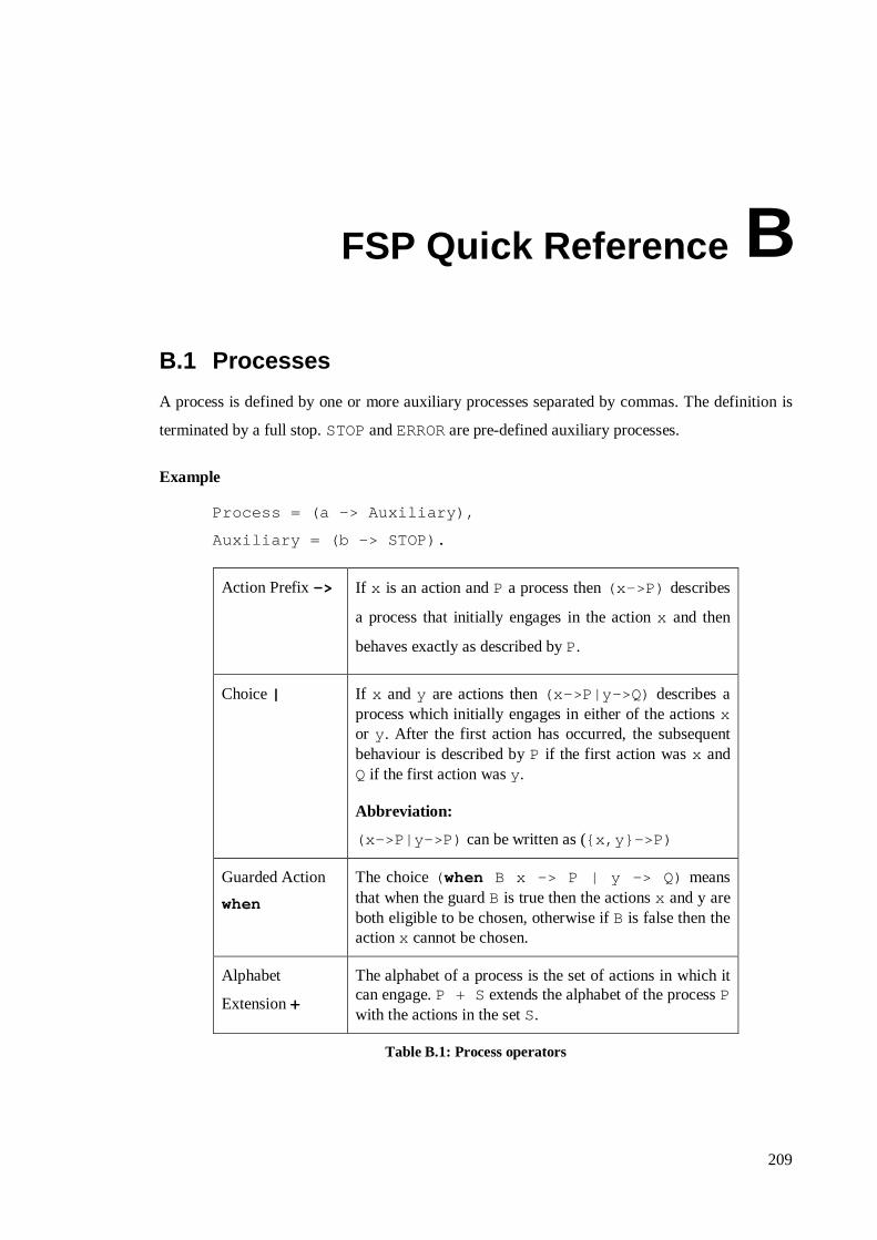
209
FSP Quick Reference B
B.1 Processes
A process is defined by one or more auxiliary processes separated by commas. The definition is
terminated by a full stop.STOPandERRORare pre-defined auxiliary processes.
Example
Process = (a -> Auxiliary),
Auxiliary = (b -> STOP).
Action Prefix-> If x is an action andP a process then(x->P) describes
a process that initially engages in the actionx and then
behaves exactly as described byP.
Choice| If x andy are actions then(x->P|y->Q) describes aprocess which initially engages in either of the actionsxor y . After the first action has occurred, the subsequentbehaviour is described byP if the first action wasx andQ if the first action wasy .
Abbreviation:
(x->P|y->P) can be written as ({x,y}->P)
Guarded Action
when
The choice( when B x -> P | y -> Q) meansthat when the guardB is true then the actionsx and y areboth eligible to be chosen, otherwise ifB is false then theactionx cannot be chosen.
Alphabet
Extension+
The alphabet of a process is the set of actions in which itcan engage.P + S extends the alphabet of the processPwith the actions in the setS.
Table B.1: Process operators

APPENDIX B FSP QUICK REFERENCE
210
B.2 Composite processes
A composite process is the parallel composition of one or more processes. The definition of a
composite process is preceded by|| .
Example
||Composite = (P || Q).
ParallelComposition||
If P and Q are processes then(P||Q) represents theconcurrent execution ofP andQ.
Replicatorforall
forall [i:1..N] P(I) is the parallelcomposition(P(1) || … || P(N))
ProcessLabelling:
a:P prefixes each label in the alphabet ofP with a.
ProcessSharing::
{a 1,..,a x}::P replaces every labeln in the alphabetof P with the labels a1.n,…,a x.n . Further, everytransition(n->Q) in the definition ofP is replaced withthe transitions({a 1.n,…,a x.n}->Q) .
Priority High << ||C =(P||Q)<<{a 1,…,a n} specifies a compositionin which the actionsa1,…,a n have higher priority thanany other action in the alphabet ofP||Q including thesilent actiontau . In any choice in this system which hasone or more of the actionsa1,…,a n labelling atransition, the transitions labelled with lower priorityactions are discarded.
Priority Low >> ||C=(P||Q)>>{a 1,…,a n} specifies a compositionin which the actionsa1,…,a n have lower priority thanany other action in the alphabet ofP||Q including thesilent actiontau . In any choice in this system which hasone or more transitions not labelled bya1,…,a n, thetransitions labelled bya1,…,a n are discarded.
Table B.2: Composite process operators
B.3 Common operators
The operators in Table B.3 may be used in the definition of both processes and composite
processes.

APPENDIX B FSP QUICK REFERENCE
211
Conditionalif then else
The processif B then P else Q behaves as theprocessP if the conditionB is true otherwise it behavesas Q. If the else Q is omitted andB is false, then theprocess behaves asSTOP.
Re-labelling/ Re-labelling is applied to a process to change the namesof action labels. The general form of re-labelling is:/{ newlabel_1/oldlabel_1,…newlabel_n/oldlabel_n}.
Restriction \ When applied to a processP, the restriction operator\{a 1..a x} removes the action namesa1..a x from thealphabet ofP and makes these concealed actions "silent".These silent actions are labelledtau . Silent actions indifferent processes are not shared.
Interface@ When applied to a processP, the interface operator@{a1..a x} hides all actions in the alphabet ofP notlabelled in the seta1..a x.
Table B.3: Common process operators
Prefix matching: The action labels in a restriction or an interface set, and those on the right-
hand side of a re-labelling pair, apply “prefix matching”. That means that they matchprefixesof
labels in the alphabet of the process to which they are applied. For example, an action labela in a
restriction set will hide all labels prefixed bya e.g. a.b, a[1], a.x.y . Similarly, the re-
labelling pairx/a will replace such labels asx.b, x[1], x.x.y . Prefix matching simplifies the
uniform manipulation of groups of labels when they share the same prefix.
B.4 Properties
Safetyproperty
property P = E defines a property which is satisfiedonly by traces accepted byE, whereE is a deterministicprocess.
Progressprogress
progress P = {a 1,a 2..a n} defines a progress
propertyP which asserts that in an infinite execution of a
target system, at least one of the actionsa1,a 2..a n will
be executed infinitely often.
Table B.4: Safety and progress properties

212

213
FSP Semantics C
C.1 Semantics of FSP
We give meaning to our basic FSP language in terms of LTSs. To do this, we define a function
lts:ÿ→℘, whereÿ is the set of FSP expressions, and℘ the set of LTSs. The functionlts is
defined inductively on the structure of FSP expressions as follows.
Take indexi to range over {1, 2, 3, …}. We use:
• E, Ei to range overÿ,
• Q, Qi to range over process identifiers,
• P to range over℘,
• B, C to range over sets of observable actions (i.e.B⊆Act, C⊆Act),
• p to range overStates-{ π}, and
• a, ai to range over observable actionsAct.
PROCESS DEFINITION : Q = E means thatlts(Q) =def lts(E)
||Q = E means thatlts(Q) =def lts(E)
PROCESS CONSTANTS: lts(STOP) =⟨{ s}, { τ}, {}, s⟩
lts(ERROR) =Π
PREFIX : if E≠ERROR, andlts(E) = ⟨S, A, ∆, q⟩, thenlts(a→E) = ⟨S∪{ p}, A∪{ a}, ∆∪{( p, a, q)},
p⟩, wherep∉S. Otherwise if (E=ERROR),lts(a→E) = ⟨{ p, π}, { a, τ}, {( p, a, π)}, p⟩, where p≠π.
CHOICE : Let 1≤ i ≤n, and lts(Ei) = ⟨Si, Ai, ∆i, qi⟩. Then lts(a1→E1 | … | an→En) = ⟨S∪{ p},
A∪{ τ} ∪1≤i≤n{ ai}, ∆∪1≤i≤n{( p, ai, qi)}, p⟩, wherep∉Si, and ,�iiSS = �i
i∆=∆ and A={a| a∈Ai ∧
Ei≠ERROR}.

APPENDIX C FSP SEMANTICS
214
ALPHABET EXTENSION : if lts(E) = ⟨S, A, ∆, q⟩, thenlts(E+B) = ⟨S, A∪B, ∆, q⟩.
RELABELLING – PRIMITIVE PROCESS : For a functionf: Act→Act, and an expressionE of a
primitive process, lts(E/f) = lts(E)/f.
RELABELLING – COMPOSITE PROCESS: For a functionf:Act→Act, and a composite process
expression (Q1||Q2||…||Qn), lts((Q1||Q2||…||Qn)/f) = lts(Q1/f) || lts(Q2/f)||…||lts(Qn/f).
RESTRICTION : lts(E\B) = lts(E)↑C, whereC = αlts(E) – B.
INTERFACE: lts(E@B) = lts(E)↑B.
COMPOSITION : lts(E1||E2) = lts(E1) || lts(E2).
PRIORITY : lts(E << B) = lts(E) << B andlts(E >> B) = lts(E) >> B.
RECURSION: Let us represent asrec(X=E) the FSP process defined by the recursive equation
X=E, whereX is a variable inE. For example, the process defined by the recursive definitionX =
(a→X) is represented asrec(X=(a→X)). We useE[X←rec(X=E)] to denote the FSP expression
that is obtained by substitutingrec(X=E) for X in E. Thenlts(rec(X=E)) is the smallest LTS that
satisfies the following rule:
PEXreclts
PEXrecXEltsa
a
→=→=←
))((
)])([(
Intuitively, any action inferred by the expressionE unwound once can also be inferred by the
process represented by the recursive definition. Mutually recursive equations can be reduced to
the simple form described above.
Note that in FSP, all recursive expressions are guarded, and composite processes cannot be
defined recursively.
SAFETY PROPERTIES: propertyQ = E, means thatlts(Q) =def image(lts(E)), where for any LTS
P=⟨S, A, ∆, p⟩, image(P) = ⟨S∪{ π}, A, ∆´, q⟩, where∆´ is defined as follows:
∆´ = ∆ ∪ {( s, a, π) | s ∈ S, a ∈ A, and∃/ s´∈ S: (s, a, s ) ∈ ∆}.
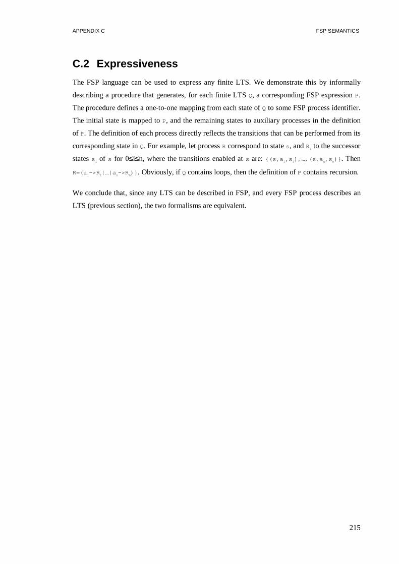
APPENDIX C FSP SEMANTICS
215
C.2 Expressiveness
The FSP language can be used to express any finite LTS. We demonstrate this by informally
describing a procedure that generates, for each finite LTSQ, a corresponding FSP expressionP.
The procedure defines a one-to-one mapping from each state ofQ to some FSP process identifier.
The initial state is mapped toP, and the remaining states to auxiliary processes in the definition
of P. The definition of each process directly reflects the transitions that can be performed from its
corresponding state inQ. For example, let processR correspond to states , andRi to the successor
statess i of s for 0≤i≤n, where the transitions enabled ats are: {(s,a 1,s 1),…,(s,a n,s n)} . Then
R=(a 1->R 1|…|a n->R n)} . Obviously, ifQ contains loops, then the definition ofP contains recursion.
We conclude that, since any LTS can be described in FSP, and every FSP process describes an
LTS (previous section), the two formalisms are equivalent.

216

217
Theorems and Proofs D
D.1 Lemmas
The lemmas presented in this section are used in the proof of the theorems of Section D.2.
L EMMA D.1: For any two processesP, T such thatαT⊆αP, tr((P||T)↑αT) = tr(P↑αT) ∩ tr(T).
Proof: Let P, T be two processes such thatαT⊆αP. Therefore, inP||T, only those transitions
labelled with actions inαT need to be synchronised, and the remaining ones are interleaved. In
(P||T)↑αT, all transitions labelled with actions that do not belong toαT becomeτ transitions. As
τ transitions do not synchronise with any other transitions, (P↑αT)||T is identicalwith (P||T)↑αT.
The reason is that in (P↑αT), the only transitions that are not labelled withτ are exactly the ones
that are labelled with actions ofαT, i.e. exactly those transitions that are synchronised with those
of T in P||T. Since (P↑αT)||T is identicalwith (P||T)↑αT), tr((P||T)↑αT) = tr((P↑αT)||T).
tr((P↑αT) ||T) =def{ t | (t α(P↑αT) ∈ tr(P↑αT)) ∧ (t αT ∈ tr(T)) ∧ (t ∈ (α(P↑αT)∪αT)*)} =
{ t | (t (αP∩αT) ∈ tr(P↑αT)) ∧ (t αT ∈ tr(T)) ∧ (t ∈ (αT)*)}= αT⊆αP
{ t ∈ (αT)* | (t ∈ tr(P↑αT)) ∧ (t ∈ tr(T))} =
{ t ∈ (αT)* | t ∈ (tr(P↑αT)∩tr(T))} = { t | t ∈ (tr(P↑αT)∩tr(T))}.
We therefore conclude that:tr((P ||T)↑αT) = tr((P↑αT)||T) = tr(P↑αT)∩tr(T). ■
L EMMA D.2: Let Z, Pbe two processes such thatαP⊆αZ. Then:Z ~ (Z||P) ⇒ tr(Z↑αP) ⊆ tr(P).
Proof: Z ~ (Z||P) ⇒ Z↑αP ∼ (Z||P)↑αP. But given that ~ is stronger than trace equivalence:
tr(Z↑αP) = tr((Z||P)↑αP) =lemmaD.1tr(Z↑αP)∩tr(P).
So we have that:

APPENDIX D THEOREMS AND PROOFS
218
Z ~ (Z||P) ⇒ (tr(Z↑αP) = tr(Z↑αP)∩tr(P)) ⇒ tr(Z↑αP) ⊆ tr(P). ■
D.2 Theorems
In this section, we present and prove the transparency theorem. This theorem is an extension of
the interface theorem, proposed by [Cheung 94c], and formulated as follows:
INTERFACE THEOREM : For two totally defined LTSsZ andP, Z ~ (Z ||P) if:
1. αP ⊆ αZ;
2. tr(Z ↑ αP) ⊆ tr(P);
3. P is deterministic and free ofτ transitions.■
The interface theorem is related to totally defined processes – the specialπ state had not been
introduced in the model at the time it was developed. We have made this explicit in the above
formulation of the theorem. In fact, the theorem is not always satisfied by processes that are not
totally defined, as shown in the example of Figure D.1.
Z
a
b
0 1
P
b
-1 0
Result
ab
-1 0
Z = (a -> Z | b -> STOP).
P = (b -> ERROR).
||Result = (Z||P).
Figure D.1: Processes that are not totally defined do not always satisfy the interface theorem.
The introduction of the transparency theorem was motivated by the need to handle user-specified
interfaces in our method, as described in Chapters 2 and 5. The transparency theorem provides
conditions that are both necessary and sufficient for the correctness of an interface. These
conditions can therefore be used in checking that user-specified interfaces are correct. In this
way, we have proven that the technique presented by [Cheung and Kramer 96b] for checking
user-specified interfaces is not conservative, but accepts exactly those interfaces that are correct.

APPENDIX D THEOREMS AND PROOFS
219
TRANSPARENCY THEOREM : Let Z and P be two totally defined processes, whereP is
deterministic and free ofτ transitions. ThenZ ~ (Z || P) iff:
1. αP ⊆ αZ;
2. tr(Z ↑ αP) ⊆ tr(P).
Proof: if part: Implied from the interface theorem.
only-if part: In this part we show that the two conditions are necessary. LetZ, P be two totally
defined processes such thatZ ~ (Z||P), whereP is a deterministic process free ofτ transitions. We
will prove that (i)αP⊆αZ and that (ii)tr(Z↑αP)⊆tr(P).
(i) Z~(Z ||P) ⇒ αZ = α(Z||P). But α(Z||P)=αZ∪αP and thereforeαZ=αZ∪αP, which implies that
αP⊆αZ.
(ii) We have shown in (i) thatαP⊆αZ. From lemma D.2, we conclude thattr(Z↑αP)⊆tr(P),
which completes the proof.■
We have tried to keep the conditions of the transparency theorem as weak as possible. This has
been managed for all, except the one that requiresP to be deterministic and free ofτ transitions.
This is the only condition that is not both necessary and sufficient. Figure D.2 depicts an
example where althoughP is non-deterministic, it is transparent to a processZ. On the other
hand, Figure D.3 illustrates an example where, although conditions 1 and 2 of the transparency
theorem are satisfied,P is not transparent toZ because it is non-deterministic.
We conclude that it is not necessary forP to be non-deterministic and free ofτ transitions for it
to be transparent to a process. However, the two conditions of the transparency theorem cannot
guarantee thatP will be transparent if it is non-deterministic. This is the reason why we have
decided to deal with interfaces that are deterministic and free ofτ transitions. We strongly
believe that this is not a limitation of our technique. Interfaces, both user-specified and
algorithmically derived, are introduced into analysis in order to alleviate the intermediate state-
explosion problem. This is achieved by including in the analysis of subsystems the behaviour
constraints imposed by their environment, in the form of interfaces. Given thatτ actions never
synchronise with other actions, they do not provide a way of reducing arbitrary interleaving of
actions. Moreover, introducing extra non-determinism into the system should be avoided. It is
therefore reasonable to expect that interface processes should be deterministic and free ofτ
transitions.
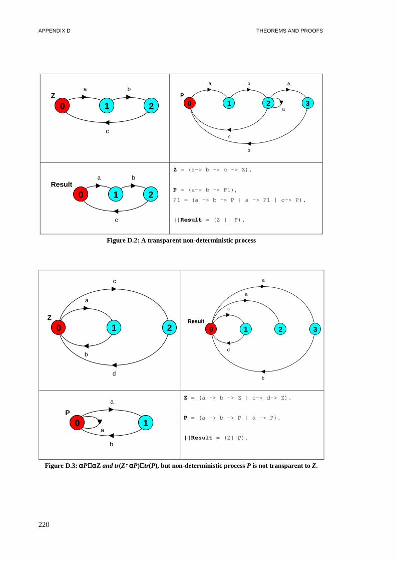
APPENDIX D THEOREMS AND PROOFS
220
Za b
c
0 1 2P
a b a
a
c
b
0 1 2 3
Resulta b
c
0 1 2
Z = (a-> b -> c -> Z).
P = (a-> b -> P1),
P1 = (a -> b -> P | a -> P1 | c-> P).
||Result = (Z || P).
Figure D.2: A transparent non-deterministic process
Z
a
c
b
d
0 1 2Result
a
a
c
d
b
0 1 2 3
P
a
a
b
0 1
Z = (a -> b -> Z | c-> d-> Z).
P = (a -> b -> P | a -> P).
||Result = (Z||P).
Figure D.3: ααααP⊆⊆⊆⊆ααααZ and tr(Z↑↑↑↑ααααP)⊆⊆⊆⊆tr(P), but non-deterministic processP is not transparent to Z.

APPENDIX D THEOREMS AND PROOFS
221
IMAGE PROCESS THEOREM: Let P and Q be two totally defined processes, whereQ is
deterministic and free ofτ transitions withαQ ⊆ αP, and letQ´ be the image process ofQ. Then
P||Q´ is totally defined ifftr(P ↑ αQ) ⊆ tr(Q).
Proof: if part: Assume thattr(P ↑ αQ) ⊆ tr(Q). But by construction ofQ´, αQ´=αQ, and
tr(Q)⊆tr(Q ). SoαQ ⊆ αP => αQ´⊆ αP, and by lemma D.1, we have that:
tr((P||Q´)↑αQ) =lemmaD.1tr(P↑αQ´) ∩ tr(Q´) ⊆ tr(Q) (sincetr(P↑αQ )⊆ tr(Q) andtr(Q)⊆tr(Q´))
We have thus proved thattr((P||Q´)↑αQ) ⊆ tr(Q) (1). But P is totally defined, so a tracet in
(P||Q´)↑αQ is undefined ifft is an undefined trace inQ´, i.e. if t∈(tr(Q´) – tr(Q)) (2). The latter
can be explained as follows. AsQ is deterministic and free ofτ transitions, and due to the way in
which Q´ is generated fromQ, the set of undefined traces ofQ´ is { t | t ∈ (tr(Q´) – tr(Q))}.
From (1), we know that the setU of undefined traces of (P||Q´)↑αQ is a subset oftr(Q). From
(2), we know thatU = { t | t ∈ (tr(Q ) – tr(Q))}. We conclude thatU is empty, and therefore
(P||Q´)↑αQ is a totally defined process. But the hiding operator cannot transform a process that
has undefined traces into one that does not, and therefore (P||Q´) is a totally defined process.
only-if part: We assume that (P||Q´) does not have undefined traces. AsQ´ is complete by
construction, we know thattr(P↑αQ´)⊆tr(Q´) (1). But if tr(P↑αQ ) contains traces in (tr(Q´) –
tr(Q)), then by the definition of the composition operator,P||Q´ contains undefined traces, which
contradicts the assumption. Therefore,tr(P↑αQ´)∩(tr(Q´) – tr(Q)) = ∅ (2). From (1) and (2) we
conclude thattr(P↑αQ) ⊆ tr(Q). ■