Model-Based Regression Trees in Economicsand the Social Sciences

Achim Zeileis

http://statmath.wu.ac.at/~zeileis/

Overview

Motivation: Trees and leavesMethodology

Model estimationTests for parameter instabilitySegmentationPruning

ApplicationsCostly journalsBeautiful professorsChoosy students

Software

Motivation: Trees

Breiman (2001, Statistical Science) distinguishes two cultures ofstatistical modeling:

Data modelsStochastic models, typically parametric.Predominant modeling strategy in economics and social sciences.Regression models are workhorse for empirical analyses.

Algorithmic modelsFlexible models, data-generating process unknown.Example: Regression trees model dependent variable Y by“learning” a partition w.r.t explanatory variables Z1, . . . ,Zl .Few applications in social sciences and especially in economics.

Motivation: Leaves

Examples for trees: CART and C4.5 in statistical and machinelearning, respectively.

Key features: Predictive power in nonlinear regression relationships,and interpretability (enhanced by visualization), i.e., no “black box”.

Typically: Simple models for univariate Y , e.g., mean or proportion.

Idea: More complex models for multivariate Y , e.g., multivariate normalmodel, regression models, etc.

Here: Synthesis of parametric data models and algorithmic treemodels.

Recursive partitioning

Base algorithm:

1 Fit model for Y .2 Assess association of Y and each Zj .3 Split sample along the Zj∗ with strongest association: Choose

breakpoint with highest improvement of the model fit.4 Repeat steps 1–3 recursively in the subsamples until some

stopping criterion is met.

Here: Segmentation (3) of parametric models (1) with additive objectivefunction using parameter instability tests (2) and associated statisticalsignificance (4).

1. Model estimation

Models: M(Y , θ) with (potentially) multivariate observations Y ∈ Yand k -dimensional parameter vector θ ∈ Θ.

Parameter estimation: θ̂ by optimization of objective function Ψ(Y , θ)for n observations Yi (i = 1, . . . , n):

θ̂ = argminθ∈Θ

n∑i=1

Ψ(Yi , θ).

Special cases: Maximum likelihood (ML), weighted and ordinary leastsquares (OLS and WLS), quasi-ML, and other M-estimators.

Central limit theorem: If there is a true parameter θ0 and given certainweak regularity conditions, θ̂ is asymptotically normal with mean θ0 andsandwich-type covariance.

2. Tests for parameter instability

Estimating function: Model deviations can be captured by

ψ(Yi , θ̂) =∂Ψ(Y , θ)

∂θ

∣∣∣Yi ,bθFluctuation tests: Systematic changes in parameters over thevariables Z = (Z1, . . . ,Zl) can be assessed by fluctuations in empiricalestimating functions.

Andrews’ supLM test for numerical Zj ,

χ2-type test for categorical Zj .

3. Segmentation

Goal: Split model into b = 1, . . . ,B segments along the partitioningvariable Zj associated with the highest parameter instability. Localoptimization of ∑

b

∑i∈Ib

Ψ(Yi , θb).

Here: B = 2, binary partitioning.

4. Pruning

Pruning: Avoid overfitting.

Pre-pruning: Internal stopping criterion. Stop splitting when there is nosignificant parameter instability.

Post-pruning: Grow large tree and prune splits that do not improve themodel fit (e.g., via crossvalidation or information criteria).

Here: Pre-pruning based on Bonferroni-corrected p values of thefluctuation tests.

Costly journals

Task: Price elasticity of demand for economics journals.

Source: Bergstrom (2001, Journal of Economic Perspectives) “FreeLabor for Costly Journals?”, used in Stock & Watson (2007),Introduction to Econometrics.

Model: Linear regression via OLS.

Demand: Number of US library subscriptions.

Price: Average price per citation.

Log-log-specification: Demand explained by price.

Further variables without obvious relationship: Age (in years),number of characters per page, society (factor).

Costly journals

agep < 0.001

1

≤ 18 > 18

Node 2 (n = 53)

●

●

●

●

●

●●

●●

●

●●●

●

●

●●

●

●

●

●

●

●

●●●

●●

●

●

●

●●

●

●

●

●

●

●●

●

●●●

●

●

●

●●

●

●● ●

−6 4

1

7

log(

subs

crip

tions

)

log(price/citation)

Node 3 (n = 127)

●

●

●●

●

●●

●

●

●

●

●

●

●●●●●●●

●

●

●

●●●

●●

●●

●●

●

●●●●●

●

●●

●●●●

●

●●

●●

●

●

●

●●

●●

●

●

●●

●

●

●●

●

●

●●

●

●●●

●

●

●●

●

●

●

●

●

●●

●

●●●

●●

●●●

●

●

●●●

●

●●

●●

●

●●

●

●

●

●

●

●

●

●

●

●

●

●

●

●

●

●●●

●

●

●

−6 4

1

7

log(

subs

crip

tions

)

log(price/citation)

Costly journals

Recursive partitioning:

Regressors Partitioning variables

(Const.) log(Pr./Cit.) Price Cit. Age Chars Society

1 4.766 −0.533 3.280 5.261 42.198 7.436 6.562

< 0.001 < 0.001 0.660 0.988 < 0.001 0.830 0.922

2 4.353 −0.605 0.650 3.726 5.613 1.751 3.342

< 0.001 < 0.001 0.998 0.998 0.935 1.000 1.000

3 5.011 −0.403 0.608 6.839 5.987 2.782 3.370

< 0.001 < 0.001 0.999 0.894 0.960 1.000 1.000

(Wald tests for regressors, parameter instability tests for partitioningvariables.)

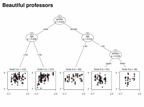
Beautiful professors

Task: Correlation of beauty and teaching evaluations for professors.

Source: Hamermesh & Parker (2005, Economics of EducationReview). “Beauty in the Classroom: Instructors’ Pulchritude andPutative Pedagogical Productivity.”

Model: Linear regression via WLS.

Response: Average teaching evaluation per course (on scale 1–5).

Explanatory variables: Standardized measure of beauty andfactors gender, minority, tenure, etc.

Weights: Number of students per course.

Beautiful professors

All Men Women

(Constant) 4.216 4.101 4.027

Beauty 0.283 0.383 0.133

Gender (= w) −0.213

Minority −0.327 −0.014 −0.279

Native speaker −0.217 −0.388 −0.288

Tenure track −0.132 −0.053 −0.064

Lower division −0.050 0.004 −0.244

R2 0.271 0.316

(Remark: Only courses with more than a single credit point.)

Beautiful professors

Hamermesh & Parker:

Model with all factors (main effects).

Improvement for separate models by gender.

No association with age (linear or quadratic).

Here:

Model for evaluation explained by beauty.

Other variables as partitioning variables.

Adaptive incorporation of correlations and interactions.

Beautiful professors

genderp < 0.001

1

male female

agep = 0.008

2

≤ 50 > 50

Node 3 (n = 113)

●

●

●

●

●

●

●●

●

●

●

●

●

●

●

●

●

●●●●

●●

●●●

●●

●

●

●

●

●

●

●●●

●

●●●

●

●

●●●

●

●

●●●●

●

●

●●●●●

●

●●●●

●

●●

●

●

●●

●

●

●

●●

●●

●●

●

●

●

●

●●

●

●●●●

●

●

●●●

●

●

●

●●●●

●

●

●

●

●

●

●

●

●●

−1.7 2.3

2

5

Node 4 (n = 137)

●

●

●

●

●●●

●

●

●

●●●

●●

●

●

●

● ●●

●

●●●

●●

●

●

●●

●●

●

●

●

●

●

●

●

●

●

●

●●

●

●●

●

●

●

●

●●

●●

●

●

●

●

●

●

●

●

●

●

●●

●

●●●●●

●

●●●●

●

●●

●●●●

●●

●

●

●

●

●

●

●

●

●

●●

●●●

●

●●●●●●●●

●●

●●●●

●

●

●●●●●

●●●●● ●

●●

●●

●

●

●

−1.7 2.3

2

5

agep = 0.014

5

≤ 40 > 40

Node 6 (n = 69)

●

●

●●

●●

●

●

●●

●●

●

●

●

●

●

●●●

●●●●●

●

●●

●

●

●

●●●

●●

●

●

●

●●

●

●●

●

●● ●

●

●

●

●

●

● ●

●

●●●●

●●●

●

●

●

●●

●

−1.7 2.3

2

5

divisionp = 0.019

7

upper lower

Node 8 (n = 81)

●

●●

●●●

●

●

●

●

●

●

●●

●

●

●

●●

●●

●

●

●●●●●

●●

●

●

●●

●

●

●

●●●●

●

●

●

●

●

●●

●●

●

●●

●●

●

●●

●

●●

●

●

●

●●●

●●●●

●

●

●

●

●

●

●

●

●

●

−1.7 2.3

2

5

Node 9 (n = 36)

●●●●●

●

●

●

●

●

●

●

●

●●

●

●

●●

●

●●

●●

●●

●

●

●

●

●●

●

●

●

●

−1.7 2.3

2

5

Beautiful professors

Recursive partitioning:(Const.) Beauty

3 3.997 0.129

4 4.086 0.503

6 4.014 0.122

8 3.775 −0.198

9 3.590 0.403

Model comparison:Model R2 Parameters

full sample 0.271 7

nested by gender 0.316 12

recursively partitioned 0.382 10 + 4

Choosy students

Task: Choice of university in student exchange programmes.

Source: Dittrich, Hatzinger, Katzenbeisser (1998, Journal of the RoyalStatistical Society C). “Modelling the Effect of Subject-SpecificCovariates in Paired Comparison Studies with an Application toUniversity Rankings.”

Model: Paired comparison via Bradley-Terry(-Luce).

Ranking of six european management schools: London (LSE),Paris (HEC), Milano (Luigi Bocconi), St. Gallen (HSG), Barcelona(ESADE), Stockholm (HHS).

Interviews with about 300 students from WU Wien.

Additional information: Gender, studies, foreign language skills.

Choosy students

italianp < 0.001

1

good poor

spanishp = 0.018

2

good poor

Node 3 (n = 8)

●

●

●

●

●

●

L P M SG B S

0

0.5Node 4 (n = 41)

●

●

●

● ●

●

L P M SG B S

0

0.5

frenchp < 0.001

5

good poor

studyp = 0.007

6

commerce other

Node 7 (n = 60)

●

●

● ●

●

●

L P M SG B S

0

0.5Node 8 (n = 105)

●

●

●

●

●●

L P M SG B S

0

0.5Node 9 (n = 89)

●

●●

● ●

●

L P M SG B S

0

0.5

Choosy students

Recursive partitioning:

London Paris Milano St. Gallen Barcelona Stockholm

3 0.21 0.13 0.16 0.07 0.43 0.01

4 0.43 0.09 0.34 0.05 0.06 0.03

7 0.33 0.42 0.05 0.06 0.09 0.04

8 0.40 0.23 0.09 0.13 0.09 0.06

9 0.41 0.10 0.08 0.16 0.16 0.09

(Standardized ranking from Bradley-Terry model.)

Software

All methods are implemented in the R system for statistical computingand graphics. Freely available under the GPL (General Public License)from the Comprehensive R Archive Network or from R-Forge:

Trees/recursive partytioning: party,

Structural change inference: strucchange,

Bradley-Terry regression/tree: prefmod2, psychotree.

http://www.R-project.org/

http://CRAN.R-project.org/

http://R-Forge.R-project.org/

Summary

Model-based recursive partitioning:

Synthesis of classical parametric data models and algorithmic treemodels.

Based on modern class of parameter instability tests.

Aims to minimize clearly defined objective function by greedyforward search.

Can be applied general class of parametric models.

Alternative to traditional means of model specification, especiallyfor variables with unknown association.

Object-oriented implementation freely available: Extension for newmodels requires some coding but not too extensive if interfacedmodel is well designed.

References

Zeileis A, Hornik K (2007). “Generalized M-Fluctuation Tests for Parameter Instability.”Statistica Neerlandica, 61(4), 488–508. doi:10.1111/j.1467-9574.2007.00371.x

Zeileis A, Hothorn T, Hornik K (2008). “Model-based Recursive Partitioning.” Journal ofComputational and Graphical Statistics, 17(2), 492–514.doi:10.1198/106186008X319331

Kleiber C, Zeileis A (2008). Applied Econometrics with R. Springer-Verlag, New York.URL http://CRAN.R-project.org/package=AER

Strobl C, Wickelmaier F, Zeileis A (2009). “Accounting for Individual Differences inBradley-Terry Models by Means of Recursive Partitioning.” Technical Report 54,Department of Statistics, Ludwig-Maximilians-Universität München.URL http://epub.ub.uni-muenchen.de/10588/