model-based guidance by the longest common subsequence algorithm for indoor autonomous vehicle...

Automation in Construction 2 (1993) 123-137 123 Elsevier

Model-based guidance by the longest common subsequence algorithm for indoor autonomous vehicle navigation using computer vision *

Ling-Ling W a n g

Institute of Computer Science, National Tsing Hua University, Hsinchu, Taiwan, ROC

Pao-Yu Ku and W e n - H s i a n g Tsai 1

Department of Computer and Information Science, National Chiao Tung University, Hsinchu, Taiwan, ROC

The use of the longest common subsequence algorithm is proposed for model-based guidance of autonomous vehicles by computer vision in indoor environments. A map of the corridor contour of a building, describing the navigation environment and measured before navigation sessions, is used as the model for guidance. Two cameras mounted on the vehicle are used as the vision sensors. The wall baselines in the images taken from the two cameras are extracted and constitute the input pattern. The environment model and the input pattern are represented in terms of line segments in a two-dimensional floor-plane world. By encoding the line segments into one-dimensional strings, the best matching between the environment model and the input pattern is just the longest common subsequence of the strings. So no complicated comparison is needed and robust matching results can be obtained. The actual position and orientation of the vehicle are determined accordingly and used for guiding the navigation of the vehicle. Successful navigation sessions on an experimental vehicle are performed and confirm the effectiveness of the proposed approach.

Keywords: Autonomous vehicle navigation; model-based guidance; longest common subsequence algorithm.

1. Introduction

R e s e a r c h and d e v e l o p m e n t of a u t o n o m o u s vehicles have a t t r ac t ed w i d e s p r e a d in te res t re- cently. This t e n d e n c y is due to the g rea t appl ica- t ion po ten t i a l of the a u t o n o m o u s vehic les and the fast d e v e l o p m e n t of c o m p u t e r vis ion techniques . Poss ible app l i ca t ions inc lude au toma t i c f reeway dr iving [8], gu idance of the b l ind and the d i sab led [6], i ndoo r safety guard ing , tour is t guid ing for s ightseeing, etc. Severa l successful a u t o n o m o u s vehic le systems have b e e n i m p l e m e n t e d for various purposes . Some of t h e m were des igned to o p e r a t e in o u t d o o r env i ronment s [1-3] , and the o the r s to o p e r a t e in indoor env i ronmen t s [4-7].

F o r o u t d o o r navigat ion , the C M U mobi le robo t

* Discussion is open until December 1993 (please submit your discussion paper to the Editor on Construction Tech- nologies, T.M. Knasel).

1 To whom correspondence should be sent.

[1], Navlab, e q u i p p e d with mul t ip le sensors , in- c luding color T V cameras , r ange sensors , iner t ia l naviga t ion sensors , odome te r s , etc., was des igned to naviga te a long the roads in a p a r k or a campus . Us ing Sun works ta t ions , the Navlab is dr iven at 10 c m / s l ike a slow shuffle. A f t e r m o u n t e d with an expe r imen ta l h igh - speed processor , the vehic le is dr iven at speed of 50 c m / s .

A n o t h e r system deve loped by T u r k et al. [2], ca l led Alvin, is e q u i p p e d with an R G B c a m e r a and a laser range scanner . T h e Alvin can s teer a r o u n d obs tac les while navigat ing on the road . S p e e d s up to 20 k m / h o u r can be achieved on a s t ra ight obs tac le - f ree road . T h e used ha rdwares inc lude a Vicom image p rocesso r and an In te l mul t ip rocesso r system.

D ickmanns and G r a e f e [3] bui l t a successful a u t o n o m o u s vehic le system, ca l led V a M o R s , using two cameras as the vision sensors , one wide- angle c a m e r a to cover a large sec tor of the envi- r o n m e n t and one t e l e c a m e r a to scrut in ize d is tan t envi ronments . Ful ly a u t o n o m o u s runs have b e e n

0926-5805/93/$06.00 © 1993 - Elsevier Science Publishers B.V. All rights reserved

124 L.-L. Wang et al. / Vehicle navigation using computer vision

performed under various road and weather con- ditions. Speeds up to 96 k m / h have been reached on a level surface. The hardware architecture contains 15 16-bit Intel 8086 processors.

For indoor navigation, reflecting tapes or white lines on the floor or ceiling may be used to guide a robot vehicle [4,5]. An alternative approach is to use underground electromagnetic guidelines which can be sensed by the magnetic coil on a vehicle [4]. Both of these approaches are less flexible.

Madarasz et al. [6] designed an autonomous wheelchair to navigate inside an office building. The on-board processor is an IBM portable PC. An ultrasonic range finder is used to detect ob- stacles and the dead-ends of corridors; a camera is used for corridor following and rooro label recognition. The precise location of the wheelchair is not attainable since only road following and rough beacon location techniques are used.

The Blanche of A T & T Bell Laboratory [7] is designed to operate inside an office or factory. The software development is performed on Sun workstations. Its navigation depends on two sensors, an optical range finder and an odometer. The odometer readings are integrated to locate the vehicle during navigation. As the vehicle con- tinues to move, the odometer errors in position and orientation tend to accumulate. To solve this problem, wall bar codes at known positions are provided. The range finder has been designed to be capable of reading such wall marks. And the environment is assumed to be obstacle free.

Indoor autonomous vehicle navigation by computer vision with the aim of low hardware cost is the main interest of this study. Emphasis is placed on the study of automatic guidance by the use of a pre-known environment model. Other tasks such as obstacle avoidance, automatic model building, and camera calibration are discussed elsewhere [8,14,17-19]. In a navigation session, the autonomous vehicle should be able to locate itself in an environment. Using a pre-learned model of the environment is a reasonable approach. Vehi- cle location can be achieved by matching the information obtained from the sensors on the vehicle with the environment model. An efficient matching method and a simple model representa- tion scheme usually are desired for real time navigation.

Tsubouchi and Yuta [9] used color images and

a stored map information to reckon a mobile robot in a corridor environment. The key step is the matching between the color image and the map information which is performed by exhaustive investigation of similar color trapezoids in both the image and the map. Yachida et al. [10] determined the robot location by matching the extracted vertical edges in the image with those in a stored model of the environment. It is necessary to estimate precisely the camera panning angle before the matching process. Crowley [11] used line segments to represent the sensor model (i.e., information obtained from a sonar ranging device) and the composite local model (i.e., information integrated from the sensor model and a pre-learned global model). The matching between the line segments of the composite local model and those of the sensor model is achieved by exhaustive pairing checking of segments' ori- entations, positions, and lengths. Chatila and Laumond [12] located the vehicle in a building using the coordinates of object vertices as the matching features. And the matching is done by exhaustive comparison of the distances between any two points in the input pattern and the environment model, respectively.

In this study, a map of the corridor contour of a building, describing the navigation environment , is set up as the model (called corridor model in the sequel). An experimental autonomous vehicle was developed for use in this research [18]. Mounted on the vehicle are two cameras which are used as the vision sensors. The wall baselines of the building corridor in the images taken from the two cameras are extracted and constitute the input pattern. The corridor model and the input pattern are represented in terms of line segments in a two-dimensional floor-plane world. By encoding the line segments into one-dimensional strings, the best matching between the corridor model and the input pattern is just the longest common subsequence (LCS) of the two strings. The matching is achieved through the use of an LCS algorithm, in which no complicated pairing comparison is needed. The time complexity of the algorithm is of the order of O(mn) where m and n are the numbers of line segments in the corridor model and the input pattern, respectively. From the matching result, the vehicle can locate itself in the environment and autonomous navigation can be per formed.

L.-L. Wang et al. / Vehicle navigation using computer vision 125

Fig. 1. An experimental three-wheel vehicle.

Figure 1 shows the outlook of the experimental autonomous vehicle. It consists of a single steerable driving wheel at the front and two pas- sive rear wheels. The vehicle dimensions are 60 cm wide and 140 cm long. The on-board processor is a P C / A T microcomputer with a PC-VI- SION-PLUS imaging interface. The two cameras mounted on the vehicle can be directed leftward and rightward, respectively, so as to take images covering a large sector of the environment.

In Section 2, the theoretical framework of the proposed model-based guidance by the LCS algorithm is introduced. Then we derive vehicle locations from LCS matching results in Section 3. The description of employed image processing

V-1 I left

camera

I image

extract left input

.pattern

I pefforrn I LCS

matching

lera ]

~V

ta c,,~t ~

~ a g e I

I

i Peff°rm 1~ LCS

matching

compute the vehicle location at the time instant of image taking

predict the vehicle location after LCS matching

I steer the vehicle [

Fig. 2. The computational framework of a navigation cycle by longest common subsequence (LCS) matching.


Li+l

initial vehicle location

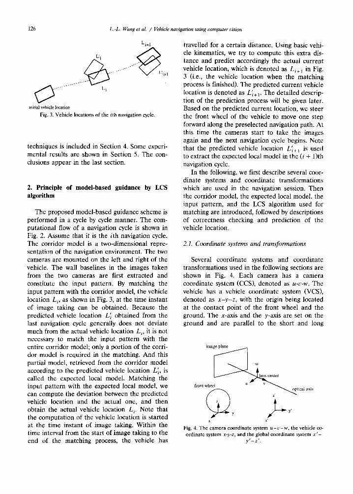
Fig. 3. Vehicle locations of the ith navigation cycle.

techniques is included in Section 4. Some experimental results are shown in Section 5. The conclusions appear in the last section.

2. Principle of model-based guidance by LCS algorithm

The proposed model-based guidance scheme is performed in a cycle by cycle manner. The computational flow of a navigation cycle is shown in Fig. 2. Assume that it is the ith navigation cycle. The corridor model is a two-dimensional repre- sentation of the navigation environment. The two cameras are mounted on the left and right of the vehicle. The wall baselines in the images taken from the two cameras are first extracted and constitute the input pattern. By matching the input pattern with the corridor model, the vehicle location L~, as shown in Fig. 3, at the time instant of image taking can be obtained. Because the predicted vehicle location L'~ obtained from the last navigation cycle generally does not deviate much from the actual vehicle location L,, it is not necessary to match the input pattern with the entire corridor model; only a portion of the corridor model is required in the matching. And this partial model, retrieved from the corridor model according to the predicted vehicle location L'~, is called the expected local model. Matching the input pattern with the expected local model, we can compute the deviation between the predicted vehicle location and the actual one, and then obtain the actual vehicle location L~. Note that the computation of the vehicle location is started at the time instant of image taking. Within the time interval from the start of image taking to the end of the matching process, the vehicle has

travelled for a certain distance. Using basic vehicle kinematics, we try to compute this extra distance and predict accordingly the actual current vehicle location, which is denoted as Li+ t in Fig. 3 (i.e., the vehicle location when the matching process is finished). The predicted current vehicle location is denoted as L'i+ 1. The detailed description of the prediction process will be given later. Based on the predicted current location, we steer the front wheel of the vehicle to move one step forward along the preselected navigation path. At this time the cameras start to take the images again and the next navigation cycle begins. Note that the predicted vehicle location L'i+l is used to extract the expected local model in the (i + 1)th navigation cycle.

In the following, we first describe several coordinate systems and coordinate transformations which are used in the navigation session. Then the corridor model, the expected local model, the input pattern, and the LCS algorithm used for matching are introduced, followed by descriptions of correctness checking and prediction of the vehicle location.

2.1. Coordinate systems and transformations

Several coordinate systems and coordinate transformations used in the following sections are shown in Fig. 4. Each camera has a camera coordinate system (CCS), denoted as u-v-w. The vehicle has a vehicle coordinate system (VCS), denoted as x - y - z , with the origin being located at the contact point of the front wheel and the ground. The x-axis and the y-axis are set on the ground and are parallel to the short and long

image plane w

~ e n t e r

front wheel u v ~ . . z' "-,,..~t~cal ax,s

x x'

Fig. 4. The camera coordinate system u - v - w, the vehicle coordinate system x-y-z, and the global coordinate system x ' -

y~-z ' .


sides of the vehicle body, respectively. To describe the environment, we need a third coordinate system, called the global coordinate system (GCS), which is denoted as x ' - y ' - z '. The x'-axis and the y'-axis are defined to lie on the ground.

The GCS is assumed to be fixed all the time while the VCS is moving with the vehicle during navigation. The location of the vehicle can be assured once the relation between the VCS and the GCS has been found. Since the vehicle moves on the ground all the time, the z-axis and the z'-axis can be ignored. That is, the relation between the two-dimensional coordinate systems x - y and x ' - y ' is sufficient to determine the position and orientation of the vehicle. The transformation between the CCS and the VCS for each camera can be written in terms of homoge- neous coordinates [8] as

(u , v, w, 1) = (x , y, z, 1)

1°°i] 0 1 0 0 1

--Yd --Zd

r l2 r13 0

r22 r23 0

r32 r33 0

0 0 1

x 0

--X d

r l l

X r21 (1) E31

0

where

r H = cos Ocos ~O + sin Osin ~bsin ~b,

r12 = - - s i n Ocos ~b,

r13 -- sin Osin ~bcos ~b - cos Osin ~O,

r21 = sin Ocos O - cos Osin ~bsin O,

r22 = COS OCOS q~,

r23 = --COS Osin ~bcos ~b - sin Osin ~b,

r31 = cos ~bsin ~,

r32 = sin ~b,

r33 = COS q~COS q/,

and 0, th, and qJ are the pan, tilt, and swing angles of the camera, respectively, with respect to the VCS; (xd, Yd, Zd) is the translation vector from the origin of the VCS to the origin of the CCS.

Y x

Fig. 5. The relation between two-dimensional coordinate systems x - y and x ' - y ' represented by a translation vector

(x~, y~) and a relative rotation angle to.

The transformation between the two two-dimensional coordinate systems x - y and x ' - y ' can be written as follows:

COS to ( x ' , y ' , l ) = ( x , y , 1) - s i n to

0 0!]1 x y;

sinto ! ] COS to

0

(2)

where (x~, y~) is the translation vector from the origin of x ' - y ' to the origin of x - y and to is the relative rotation angle of x - y with respect to x ' -y ', as shown in Fig. 5. The vector (x~, y~) and the angle to determine the position and orientation of the vehicle in the GCS, respectively. In the following, the combination of the vehicle position and orientation is referred to as the vehicle

t ¢ location and is denoted by a triplet (Xp, yp, to).

2.2. The corridor model

The goal of this study is to achieve autonomous vehicle guidance in a corridor environment. The corridor environment and the global navigation path are assumed to be known in advance. Shown in Fig. 6 is the top view of the wails of the corridor in the building in which the experiments for this research is conducted. It is time-consuming and not necessary to match the entire corridor model with the sensor input pattern. Matching with the expected local model is sufficient. The expected local model can be extracted from the corridor model according to the


1

1 Fig. 6. Top view of the walls of a corridor in a building,

1--"] visible

Fig. 8. An illustration of the region on the ground visible to the camera bounded by the border lines Q1 through Q4-

predicted vehicle location computed from the last navigation cycle.

The way we use to extract the expected local model is to find first the intersection lines of the ground and the bounding planes of the field of view of each camera on the vehicle, and compute then the portion of the corridor model appearing within the field of view. The bounding planes, denoted as P1 through P4, are shown in Fig. 7 and the intersection lines, denoted as Q1 through Q4, are shown in Fig. 8.

The equations of Pt through P4 in the CCS are

P1: u = tan(/3t/2)v,

P2: u = - t a n ( / 3 t / 2 ) v ,

P3: w = tan(/32/2)v,

P4: w = - tan(/32/Z)v,

where 31 and ~[~2 a r e the view angles of each camera in the horizontal and in the vertical directions, respectively.

Substituting eqn. (1) into the preceding equations and letting z = 0, we get the equations of QI through Q4 in the VCS. These equations are

~ plane P2

arnera p l ~ p 1 ~ ~ ~ , ~

plane P4 Fig. 7. The field of view of acamera and its bounding planes.

then transformed into the GCS using eqn. (2) and the predicted vehicle location. The corridor model and the intersection lines Qt through Q4 are all on the ground plane and are now all described in the GCS. Q1 through Q4 can then be used to determine which line segments of the corridor model are visible from the views of the cameras. The clipping algorithm using region coding proposed by Cohen and Sutherland [15] is employed for this purpose. The line segments within the fields of cameras' views after clipping constitute the expected local model. In addition, we take/31 and /3 2 to be several degrees larger than the actual values so as to accommodate possible errors of the predicted vehicle location.

Note that the foregoing extraction process is repeated for each of the two cameras. So the expected local model consists of two parts: the left expected local model and the right expected local model.

2.3. The input pattern

The input pattern is a description of the local environment obtained from the cameras on the vehicle. In this study, we use the wall baselines at the bottom of the baseboards of the corridor wails, as shown in Fig. 9, to describe the corridor environment. They are line patterns in the images taken from the cameras and are easy to detect. The detected baseline points in the images are first backprojected onto the ground in the VCS using the camera-to-vehicle transformation matri- ces obtained from a pre-performed camera calibration process [14]. By the vehicle location pre-

L.-L. Wang et a L / Vehicle navigation using computer vision 129

bols from the string. For example, 'bcd' is a subsequence of 'abacd'. A common subsequence of two strings is a subsequence of both strings and a longest common subsequence (LCS) is one with the greatest length. For example, 'tony' is an LCS of 'entropy' and 'topology'. The LCS problem can be solved by dynamic programming [13], and an algorithm is listed below.

Fig. 9. A picture showing the wall baselines of the corridor in a building.

dicted at the last navigation cycle and eqn. (2), the baseline points in the VCS can be transformed further into the GCS. These points are then traced and grouped into line segments and the result is called the input pattern. The detailed implementation process of grouping points into line segments is discussed in Section 4. Like the expected local model, the input pattern is com- posed of two parts: the left input pattern and the right input pattern. The input pattern is represented as a set of two-dimensional line segments on the ground, therefore the matching of the expected local model and the input pattern is two-dimensional in nature and the computation time is so reduced.

2.4. LCS matching

An LCS algorithm [13] is used in this study to match the expected local model and the input pattern to obtain their deviation. LCS detection is a well known problem which is found in many applications, such as detection of data redun- dancy or information lost. It is a new idea to apply the LCS concept to autonomous vehicle guidance. In the following, we first briefly intro- duce the LCS problem and then describe how to apply an LCS algorithm to match the expected local model with the input pattern for the guidance purpose.

In the LCS problem, the inputs are of the form of strings. A string is a sequence of symbols, such as integers or English letters. A subsequence of a string is obtained be deleting zero or more sym-

Algorithm. LCS detection Input. Two strings A =a~az..a m and B =

blb2..b n. Output. The LCS S of A and B. Step 1. Create an array L with a dimension of

m b y n. Step 2. F o r i f r o m 0 t o m

set L(i, 0) = 0; and for j from 0 to n

set L(0, j ) = 0. Step 3. For i from l to m and

for j from 1 to n if a i =b~,

then set L(i, j ) = L(i - 1, j - 1 ) + 1 else if L(i, j - 1) > L(i - 1, j),

then set L(i, j ) = L(i, j - 1) else set L(i, j ) = L ( i - 1, j).

Step 4. S e t i = m ; j = n ; a n d k = O ; while i ~ 0 and j ~ O,

if L(i, j ) = L(i, j - 1), then set j = j - 1 else if L(i, j ) = L ( i - 1, j),

then set i = i - 1 else set S(k) -- ai; k = k + 1; i = i - 1; and j = j - 1.

Step 5. Reverse S.

It is natural to regard the expected local model and the input pattern as strings and use the LCS of the strings as their best match. To code the baselines of the corridor model and the input pattern into strings, we first d ivide them into short line segments. For each short line segment with its direction closer to verticality, it is coded as '1'; otherwise, it is coded as '0'. Note that the corridor model consists of only vertical and horizontal line segments, so the two codes 0 and 1 are sufficient. It is necessary to match the left ex-

130 L.-L. Wang et aL / Vehicle navigation using computer vision

l (a) A rlght expected local model coded to be 111111111111111100011111.

\

correct the predicted vehicle location (L~ in Fig. 3) in the GCS according to the following process. First rotate the predicted vehicle location through the angle value of y with respect to the reference point R, and then translate it through the values of (tx, ty). Note that if we rotate and translate the input pattern in the same way, the corridor model and the input pattern will overlap.

3.2. Vehicle location at the end of the matching process

(b) A right input pattern coded to be 11 l I 1111111100011 l I 111.

Fig. 10. An example of coding two-dimensional line segments to be one-dimensional strings.

pected local model with the left input pattern and match the right expected local model with the right input pattern, respectively. An example is shown in Fig. 10, where Fig. 10(a) is a right expected local model coded to be 111111111111111100011111 and Fig. 10(b) is a right input pattern coded to be 1111111111110001111111; the LCS of these two strings is 11111111111100011111.

3. Vehicle location from LCS matching results

3.1. Vehicle location at the time instant of image taking

The expected local model and the input pattern are represented in terms of short line segments on a two-dimensional ground plane. For each matching pair of short line segments in the expected local model and the input pattern, respectively, the deviation between them can be represented as a two-dimensional translation and a rotation with respect to a certain reference point. From all the matching pairs, we can compute an average deviation between the expected local model and the input pattern. And a refined average is computed further to increase accuracy using only those pairs whose deviations are close to the overall average.

From the computed average deviation between the expected local model and the input pattern, including a translation (tx, ty) and a rotation y with respect to a reference point R, we can

From the time instant of image taking to the end of the matching process, the vehicle has traveled a little farther. So the vehicle location obtained from correcting the predicted location using the matching result is not the real current vehicle location (Li+ 1 in Fig. 3). Instead, it is the vehicle location at the start of the matching process (or approximately at the time instant of image taking) (L i in Fig. 3). Using the speed and the front wheel direction of the vehicle, we can predict the current vehicle location by basic vehicle kinematics. By the predicted vehicle location (L'i+ 1 in Fig. 3) in the environment, a table look-up control strategy derived in [18] is used to steer the front wheel to guide the vehicle to move along a desired navigation path.

The prediction of the current vehicle location after the matching process by vehicle kinematics is derived in the following. First, we define the turn angle of the front wheel of the vehicle to be zero when the front wheel is parallel to the long side of the vehicle body. It follows from basic kinematics that the vehicle will move along a circular path if the front wheel is fixed at a specific angle other than zero. In such a case the rotation center is located at the intersection of the line perpendicular to the front wheel and that perpendicular to the rear wheels. Figure 11 shows this situation. The distance between the front wheel and the rear ones can be measured manu- ally and is denoted as d. The radius of rotation can be found to be

d r = sin 3 (3)

where 6 is the turn angle of the front wheel. Shown in Fig. 12 are the relative locations of

the vehicle before and after the matching pro-

L.-L. Wang et aL / Vehicle navigation using computer vision 131

circular path

r

rotation :enter

Fig. 11. The front wheel of the vehicle traversing a circular path.

the components of T with respect to the GCS can be found to be

T x' = T : o s oJ i - Tysin wi,

Ty' = T~sin o~ i + Tycos oJ i.

The predicted current vehicle location L'~+ 1 can thus be found to be

x:+, = x: + L ,

Y:+, : Y : + T / ,

and

O')i+ 1 ~--" ('Oi at- 'Y' if the front wheel turns rightward,

o r

(.Oi+ 1 ~--- O) i -- ~/, i f t h e f r o n t w h e e l t u r n s l e f t w a r d .

cess. Vehicle location L i is the actual vehicle location at image taking and let it be represented by (x;, y;, oh). Vehicle location L'i+ t is the predicted location after the matching process and let it be represented by (x '+ 1, Y[+ 1, OJi+ 1 )" Note that both locations L i and L'i+ 1 are with respect to the GCS. Let At to be the time interval from the time instant of image taking to the end of the matching process. It can be found by querying the system clock, and the current direction 6 of the front wheel can be obtained from the control interface. Let the vehicle speed be v. We can find the turn angle 3/ of the vehicle shown in Fig. 12 to be

v a t sin 6 Y= d

because

d v A t = r y = y .

sin 6

Obviously, the length of the translation vector T of the vehicle shown in Fig. 12 can be computed to be

T 2 = r 2 + r 2 - 2r 2 cos 3'

or T = r~/e(1 - cos y)

and the direction of T with respect to the VCS at location L i is /x --- ~ r / 2 - 8 - y / 2 . Vector T with respect to the VCS at location L i c a n thus be found to be ( T x, Ty) --- (T cos /z, T sin Ix). Hence

4. Image processing techniques

The basic requirement behind the proposed approach is to represent the expected local model and the input pattern in terms of one-dimensional strings. The expected local model is a set of two-dimensional line segments, as shown in Fig. 6, either vertical or horizontal. Each line segment in the expected local model is first divided into short line segments with an identical length. Each vertical short line segment is assigned the symbol '1', and each horizontal short line segment is assigned '0'. Then the left and right expected local models can be respectively represented by one-dimensional strings. The order of each symbol in the string is determined according to the distance between the central point of the corresponding short line segment and the origin of the VCS.

For the input pattern, it is also necessary to divide the line segments into short ones and assign the symbols '1' and '0' to them. We describe hereinafter the image processing techniques for extracting the baseline points from the images and grouping them into line segments to compose the input pattern.

4.1. Extraction and backprojection o f baseline points

Two images of the baselines are taken in each navigation cycle. The images are processed and


the pixels on the baselines are extracted. This is achieved through simple scanning of each image column from left to right. Since the baselines of the wails are black and contrast well with the white floor, a threshold value may be preselected to find candidate pixels in column scanning. The scanning starts from the bottom of a column and proceeds upward. Two consecutive pixels with gray values less than the threshold value indicate a candidate pixel on a baseline. In practice, how- ever, strong lighting near the windows will cause the failure of the scanning if only a fixed threshold value is used for thresholding the entire input image. So, we divide the image into several horizontal strips and decide for each strip a threshold value according to the average gray value of the strip. The average gray value of a strip is computed by sampling the strip for every ten pixels in both horizontal and vertical directions. Only pixels corresponding to the ground and the wall are considered in computing the average gray value of a strip. So, a sampled pixel with a gray value less than a certain value, denoting a black point, is ignored.

To speed up the scanning process, a locality property is utilized. That is, if a candidate pixel is found to be at row j on column i, then the range from row j - 5 to row j + 5 on column i + 1 is scanned first. If this scanning fails to find a candidate pixel, rescanning from the lowest row is performed on column i + 1. Usually, the hit ratio is very high and the processing speed becomes much faster.

Once the candidate baseline pixels are found, they are backprojected according to eqn. (1) (using pre-calibrated camera parameters) onto the ground in the VCS. By the predicted vehicle location and eqn. (2), they can be transformed into points in the GCS.

4.2. Grouping baseline points into line segments

We associate each baseline point P in the GCS with the direction of a line segment formed from the vicinal points of P by least-square-error fitting. Then the adjacent baseline points with similar directions are grouped into a line segment also by least-square-error fitting. These line segments in the input pattern are then divided into shorter ones, each of which is coded to symbol '1'

Y . f

r

y'

l D-- ×~

Fig. 12. The vehicle location at image taking and that after the matching process.

or '0' depending on its direction, as described previously.

5. Experimental results

In the experiments, the vehicle location with respect to the GCS are computed for navigation. Shown in Figs. 13 through 15 are examples to show the effectiveness of the proposed matching approach. Figure 13(a) shows two images taken from the two cameras. Bright points in this figure indicate the found candidate pixels on the baselines. The expected local model and the input pattern are illustrated in the left and right parts of Fig. 13(b), respectively. Figure 13(c) shows the superimposition of the expected local model over the input pattern before matching. From the LCS matching result, the deviation between the corridor model and the input pattern, including a translation vector (tx, ty) and a rotation 7, can be computed. By rotating and translating the input pattern through the values of (t x, ty) and 7, respectively, we can see the matching effect of the corridor model and the input pattern, as shown in Fig. 13(d). Because of the errors from the image processing and camera calibration processes, there may exist a little deviation between the expected local model and the rotated and trans- lated input pattern. Figures 14 and 15 show two additional examples. These figures demonstrate the ability of the LCS algorithm in matching noisy


patterns. Note that in these cases, some of the points on the baselines are not detected and some points not on the baselines are detected. The actual vehicle locations obtained by manual

measurements, the predicted vehicle locations, and the computed vehicle locations from the matching results of 5 cases (including Figs. 13 through 15 as the first two and the last) are listed

(b)

(el !ct!

Fig. 13. An LCS matching result (case 1): (a) Two images taken from the two cameras; (b) The expected local model (left) and the input pattern (right); (c) Superimposition of the expected local model and the input pattern before matching; and (d) Superimposi-

tion of the expected local model and the input pattern after matching.

134 L.-L. Wang et al. / Vehicle navigation using computer eision

in Tab le 1. A l t h o u g h t h e r e a re some degrees of e r rors in the p r e d i c t e d vehicle locat ions, by the LCS match ing the vehic le loca t ion can be cor-

r ec ted to r a the r high accuracy. T h e average distance e r ro r in the x-axis d i rec t ion is about 4 cm and that in the y-axis d i rec t ion is about 10 cm.




And the average direction error is about 0.5 degree. Such errors are found to be tolerable for vehicle guidance in our navigation experiments.

1 / ~i!ii~!i i~ ̧̧̧ i

Many successful navigations have been performed on an obstacle-free corridor and the vehicle is driven at the speed of about 10 cm/s .

/b)



136 L.-L. Wang et aL / Vehicle navigation using computer vision

Table 1 Experimental results for vehicle location

actual predicted computed vehicle location vehicle location vehicle location (cm, cm, degree) (cm, cm, degree) (cm, cm, degree)

1 (122, - 1753, 8.13) (101, - 1744, 12) (126.48, - 1744.68, 8.30) 2 (120, -855, -4.34) (140, - 900, - 11) (121.67, -848.10, -4.55) 3 (110, -808, -7.51) (120, - 840, - 5 ) (105.21, -786.53, - 6.15) 4 (139, -672, 10.23) (110, - 630, 4) (137.52, -664.42, 9.33) 5 (130, -596, 2.92) (120, - 612, - 2 ) (135.82, -590.10, 3.20)

Approximately 6 seconds are needed for a navigation cycle.

6. Conclusions

In this paper, we have proposed the use of model matching by the LCS algorithm for autonomous vehicle guidance and tested it on an experimental vehicle. Accurate global location of the vehicle with respect to the environment is achieved through continuous model matching during navigation. Backprojection using the as- sumption of ground flatness and the choice of the corridor ground contour as the model simplify the matching. Only simple data structures are used to represent the environment and provide necessary information for the navigation task. The use of the LCS concept in the matching process has been verified as a reliable method for vehicle location. It is suited for this application because of its simple computation requirement and its insensitivity to noise. Satisfactory autonomous navigation results have been obtained. In spite of the low speed of navigation, we feel that the system's performance is satisfactory using only one microcomputer and some basic equipments.

Acknowledgment

This work was supported by National Science Council, Republic of China under Grant NSC79- 0404-E009-18.

References

[1] C. Thorpe, M.H. Herbert, T. Kanade and S.A. Sharer, Vision and navigation for the Carnegie-Mellon Navlab, IEEE Trans. on Pattern Analysis and Machine Intelligence, 10 (May 1988) 362-373.

[2] M.A. Turk, D.G. Morgenthaler, K.D. Gremban and M. Marra, VITS--a vision system for autonomous land vehicle navigation, IEEE Trans. on Pattern Analysis and Machine Intelligence, 10 (May 1988) 342-361.

[3] E.D. Dickmanns and V. Graefe, Applications of dynamic monocular machine vision, Machine Vision and Applica- tions, 1 (1988) 241-261.

[4] T. Tsumura, Survey of automated guided vehicle in Japanese factory, Proc. IEEE Int. Conf. on Robotics and Automation, San Francisco, CA (April 1986) 1329-1334.

[5] K.C. Drake, E.S. Mcvey and R.M. Inigo, Experimental position and ranging results for a mobile robot, IEEE J. Robotics and Automation, RA-3 (February 1987) 31-42.

[6] R.L. Madarasz, L.C. Heiny, R.F. Cromp and N.M. Mazur, The design of an autonomous vehicle for the disabled, IEEE J. Robotics and Automation, RA-2 (September 1986) 117-126.

[7] IJ . Cox, Blanche: an autonomous robot vehicle for struc- tured environments, Proc. IEEE Int. Conf. on Robotics and Automation, Philadelphia, PA (April 1988) 978-982.

[8] L.L. Wang and W.H. Tsai, Car safety driving aided by 3-D image analysis techniques, MIST Technical Report, TR-MIST-86-004, National Chiao Tung University, Hsinchu, Taiwan, R.O.C., July 1986.

[9] T. Tsubouchi and S. Yuta, Map assisted vision system of mobile robots for reckoning in a building environment, Proc. IEEE Int. Conf. on Robotics and Automation, Releigh, NC (April 1987) 1978-1984. M. Yachida, T. Ichinose and S. Tsuji, Model-guided monitoring of a building environment by a mobile robot, Proc. Int. Joint Conf. on Artificial Intelligence, Karlsruhe, West Germany, (August 1983) 1125-1127. J.L. Crowley, Navigation for an intelligent mobile robot, IEEE J. Robotics and Automation, RA-1 (March 1985) 31-41. R. Chatila and J.P. Laumond, Position referencing and consistent world modeling for mobile robots, Proc. IEEE Int. Conf. on Robotics and Automation, St. Louis, Mis- souri, (March 1985) 138-145. D.S. Hirschberg, A linear space algorithm for computing maximal common subsequences, Communications of the ACM, 18 (June 1975) 341-343. L.L. Wang and W.H. Tsai, Computing camera parameters using vanishing line information from a rectangular parallelepiped, Machine Vision and Applications, 3 (Summer 1990) 129-141. D. Hearn and M.P. Baker, Computer Graphics, Prentice- Hall, Englewood Cliffs, NJ (1986).

[10]

[111

[12]

[131

[141

[151

L.-L. Wang et aL / Vehicle navigation using computer vision 137

[16] C.F. Gerald, Applied Numerical Analysis, Addison-Wes- ley, Reading, MA (1983).

[17] L.L. Wang and W.H. Tsai, Collision avoidance by a modified least-mean-square-error classification scheme for indoor autonomous land vehicle navigation, Proceed- ings of the First Int. Conf. on Automation Technology, Taiwan, R.O.C. (July 1990) 500-510.

[18] S.Y. Chen, L.L. Wang, M.S. Chang, P.Y. Ku and W.H. Tsai, Autonomous vehicle guidance by computer vision, NSC Technical Report No. NSC77-0404-E009-31, Na-

tional Chiao Tung University, Hsinchu, Taiwan, R.O.C., 1989.

[19] S.Y. Chen, R. Lee, L.L. Wang, W.J. Ke, P.Y. Ku and W.H. Tsai, Autonomous vehicle guidance by computer vision (II), NSC Technical Report No. NSC79-0404-E009- 18, National Chiao Tung University, Hsinchu, Taiwan, R.O.C., 1990.

model-based guidance by the longest common subsequence algorithm for indoor autonomous vehicle...

Documents